Modeling, Dynamics, and Control of Tethered Satellite Systems€¦ · Tethered satellite systems...

Modeling, Dynamics, and Control of Tethered Satellite Systems

Joshua R. Ellis

Dissertation submitted to the Faculty of theVirginia Polytechnic Institute and State University

in partial fulfillment of the requirements for the degree of

Doctor of Philosophyin

Aerospace Engineering

Christopher D. Hall, ChairCraig A. WoolseyMayuresh J. PatilScott L. Hendricks

March 23, 2010Blacksburg, Virginia

Keywords: tethered satellite systems, verification and validation, finite element method,Floquet theory, sliding mode control.

Copyright 2010, Joshua R. Ellis

Modeling, Dynamics, and Control of Tethered Satellite Systems

Joshua R. Ellis

(ABSTRACT)

Tethered satellite systems (TSS) can be utilized for a wide range of space-based applica-tions, such as satellite formation control and propellantless orbital maneuvering by means ofmomentum transfer and electrodynamic thrusting. A TSS is a complicated physical systemoperating in a continuously varying physical environment, so most research on TSS dynamicsand control makes use of simplified system models to make predictions about the behaviorof the system. In spite of this fact, little effort is ever made to validate the predictions madeby these simplified models.

In an ideal situation, experimental data would be used to validate the predictions madeby simplified TSS models. Unfortunately, adequate experimental data on TSS dynamicsand control is not readily available at this time, so some other means of validation mustbe employed. In this work, we present a validation procedure based on the creation of atop-level computational model, the predictions of which are used in place of experimentaldata. The validity of all predictions made by lower-level computational models is assessedby comparing them to predictions made by the top-level computational model. In additionto the proposed validation procedure, a top-level TSS computational model is developed andrigorously verified.

A lower-level TSS model is used to study the dynamics of the tether in a spinning TSS.Floquet theory is used to show that the lower-level model predicts that the pendular motionand transverse elastic vibrations of the tether are unstable for certain in-plane spin ratesand system mass properties. Approximate solutions for the out-of-plane pendular motionare also derived for the case of high in-plane spin rates. The lower-level system model is alsoused to derive control laws for the pendular motion of the tether. Several different nonlinearcontrol design techniques are used to derive the control laws, including methods that canaccount for the effects of dynamics not accounted for by the lower-level model. All of theresults obtained using the lower-level system model are compared to predictions made by thetop-level computational model to assess their validity and applicability to an actual TSS.

Contents

1 Introduction 1

1.1 A Brief History of Tethered Satellite Systems . . . . . . . . . . . . . . . . . 1

1.2 Fundamentals of Spinning and Electrodynamic Tethered Satellite Systems . 4

1.2.1 Spinning Tethered Satellite System . . . . . . . . . . . . . . . . . . . 4

1.2.2 Electrodynamic Tethered Satellite System . . . . . . . . . . . . . . . 7

1.3 Review of Relevant Literature . . . . . . . . . . . . . . . . . . . . . . . . . . 10

1.3.1 Spinning Tethered Satellite Systems . . . . . . . . . . . . . . . . . . . 11

1.3.2 Electrodynamic Tethered Satellite Systems . . . . . . . . . . . . . . . 12

1.3.3 Spinning Electrodynamic Tethered Satellite Systems . . . . . . . . . 18

1.4 Contributions of the Present Study . . . . . . . . . . . . . . . . . . . . . . . 19

1.4.1 Validation of Computational Models . . . . . . . . . . . . . . . . . . 19

1.4.2 Verification of Computational Models . . . . . . . . . . . . . . . . . . 21

1.4.3 Dynamics of Spinning Tethered Satellite Systems . . . . . . . . . . . 21

1.4.4 Control of Spinning Tethered Satellite Systems . . . . . . . . . . . . . 22

1.5 Organization of the Dissertation . . . . . . . . . . . . . . . . . . . . . . . . . 22

2 Validation of Computational Models 23

2.1 Fundamental Concepts of System Modeling . . . . . . . . . . . . . . . . . . . 23

2.1.1 Conceptual Model . . . . . . . . . . . . . . . . . . . . . . . . . . . . 24

2.1.2 Mathematical Model . . . . . . . . . . . . . . . . . . . . . . . . . . . 25

2.1.3 Computational Model . . . . . . . . . . . . . . . . . . . . . . . . . . 25

iii

2.2 Validation of Computational Models in the Absence of Experimental Data . 26

2.3 Application of the Proposed Validation Procedure . . . . . . . . . . . . . . . 30

3 Top-Level System Model 31

3.1 Physical System and Conceptual Model . . . . . . . . . . . . . . . . . . . . . 31

3.2 Mathematical Model . . . . . . . . . . . . . . . . . . . . . . . . . . . . . . . 32

3.2.1 Coordinate Frames and Kinematics . . . . . . . . . . . . . . . . . . . 33

3.2.2 Tether Geometry and Constitutive Relation . . . . . . . . . . . . . . 36

3.2.3 Magnetic Field Model and Electrodynamic Force . . . . . . . . . . . 39

3.2.4 Equations of Motion of A . . . . . . . . . . . . . . . . . . . . . . . . 40

3.2.5 Equations of Motion of the Tether . . . . . . . . . . . . . . . . . . . . 42

3.2.6 Equations of Motion of B . . . . . . . . . . . . . . . . . . . . . . . . 46

3.2.7 Summary of the Mathematical Model . . . . . . . . . . . . . . . . . . 47

3.3 Computational Models . . . . . . . . . . . . . . . . . . . . . . . . . . . . . . 48

3.3.1 Assumed Modes Method . . . . . . . . . . . . . . . . . . . . . . . . . 48

3.3.2 Finite Element Method . . . . . . . . . . . . . . . . . . . . . . . . . . 52

3.4 Verification of Computational Models . . . . . . . . . . . . . . . . . . . . . . 59

3.4.1 The Method of Manufactured Solutions . . . . . . . . . . . . . . . . . 60

3.4.2 Finite Element Method . . . . . . . . . . . . . . . . . . . . . . . . . . 63

3.4.3 Assumed Modes Method . . . . . . . . . . . . . . . . . . . . . . . . . 66

3.5 Comparison of Computational Models . . . . . . . . . . . . . . . . . . . . . 72

3.6 Examples of Computational Model Output . . . . . . . . . . . . . . . . . . . 73

3.6.1 Example 1: Spinning Tethered Satellite System . . . . . . . . . . . . 73

3.6.2 Example 2: Electrodynamic Tethered Satellite System . . . . . . . . 83

3.7 Summary of the Top-Level System Model . . . . . . . . . . . . . . . . . . . . 92

4 Dynamics of Spinning Tethered Satellite Systems 93



iv

4.2.1 Coordinate Frames and Kinematics . . . . . . . . . . . . . . . . . . . 94

4.2.2 Tether Geometry . . . . . . . . . . . . . . . . . . . . . . . . . . . . . 96

4.2.3 Pendular Equations of Motion . . . . . . . . . . . . . . . . . . . . . . 97

4.2.4 Transverse Vibration Equations of Motion . . . . . . . . . . . . . . . 98

4.2.5 Nondimensional Equations of Motion . . . . . . . . . . . . . . . . . . 101

4.3 Computational Model: Pendular Motion of the Tether . . . . . . . . . . . . . 103

4.3.1 Solution for In-Plane Motion . . . . . . . . . . . . . . . . . . . . . . . 104

4.3.2 Floquet Analysis of Out-of-Plane Motion . . . . . . . . . . . . . . . . 108

4.3.3 Approximate Solution for Out-of-Plane Motion for Large h . . . . . . 115

4.3.4 Bounds on Out-of-Plane Motion . . . . . . . . . . . . . . . . . . . . . 125

4.3.5 Summary of Computational Predictions . . . . . . . . . . . . . . . . 129

4.4 Computational Model: Transverse Vibrations of the Tether . . . . . . . . . . 130

4.4.1 Analysis Using Separation of Variables . . . . . . . . . . . . . . . . . 130

4.4.2 Solution for the Mode Shapes . . . . . . . . . . . . . . . . . . . . . . 132

4.4.3 Floquet Analysis . . . . . . . . . . . . . . . . . . . . . . . . . . . . . 134

4.4.4 Summary of Computational Predictions . . . . . . . . . . . . . . . . 136

4.5 Validation of the Computational Model . . . . . . . . . . . . . . . . . . . . . 139

4.5.1 Pendular Motion of the Tether . . . . . . . . . . . . . . . . . . . . . . 139

4.5.2 Transverse Vibrations of the Tether . . . . . . . . . . . . . . . . . . . 148

4.5.3 Analysis of Modeling Assumptions . . . . . . . . . . . . . . . . . . . 153

4.6 Summary . . . . . . . . . . . . . . . . . . . . . . . . . . . . . . . . . . . . . 157

5 Control of Spinning Tethered Satellite Systems 160



5.3 Computational Model: Control of Pendular Motion . . . . . . . . . . . . . . 163

5.3.1 Controllability Using Electrodynamic Forcing . . . . . . . . . . . . . 163

5.3.2 Planar Trajectory Tracking . . . . . . . . . . . . . . . . . . . . . . . 166

5.3.3 Planar H Tracking . . . . . . . . . . . . . . . . . . . . . . . . . . . . 170

v

5.3.4 Sliding Mode Control . . . . . . . . . . . . . . . . . . . . . . . . . . . 172

5.3.5 Adaptive Sliding Mode Control . . . . . . . . . . . . . . . . . . . . . 181

5.4 Validation of Computational Model . . . . . . . . . . . . . . . . . . . . . . . 184

5.4.1 Planar H Tracking . . . . . . . . . . . . . . . . . . . . . . . . . . . . 188

5.4.2 Sliding Mode Control . . . . . . . . . . . . . . . . . . . . . . . . . . . 192

5.4.3 Adaptive Sliding Mode Control . . . . . . . . . . . . . . . . . . . . . 195

5.5 Summary . . . . . . . . . . . . . . . . . . . . . . . . . . . . . . . . . . . . . 196

6 Summary and Recommendations for Future Work 200

6.1 Summary of Contributions . . . . . . . . . . . . . . . . . . . . . . . . . . . . 200

6.2 Recommendations for Future Work . . . . . . . . . . . . . . . . . . . . . . . 204

Bibliography 206

vi

List of Figures

1.1 Illustrations of the various aspects of spinning TSS dynamics . . . . . . . . . 6

1.2 Illustrations of the operational principles of an electrodynamic tether system 8

2.1 Diagram of the system modeling hierarchy . . . . . . . . . . . . . . . . . . . 24

2.2 Diagram illustrating the ideal situation for computational model validation . 27

2.3 Diagram illustrating the computational model validation procedure for thecase of no experimental data . . . . . . . . . . . . . . . . . . . . . . . . . . . 29

3.1 Diagram of top-level system model . . . . . . . . . . . . . . . . . . . . . . . 33

3.2 Diagram illustrating orientation of FE relative to FO . . . . . . . . . . . . . 36

3.3 Diagram illustrating the relationship between the unstretched and stretchedtether . . . . . . . . . . . . . . . . . . . . . . . . . . . . . . . . . . . . . . . 37

3.4 Geometry of the unit dipole axis u . . . . . . . . . . . . . . . . . . . . . . . 39

3.5 Free-body diagram of a stretched differential tether length element ds . . . . 45

3.6 Plot of element shape functions N ei . . . . . . . . . . . . . . . . . . . . . . . 57

3.7 Plot of global shape functions Nj for odd j . . . . . . . . . . . . . . . . . . . 58

3.8 Plot of global shape functions Nj for even j . . . . . . . . . . . . . . . . . . 58

3.9 Discretization error as a function of normalized finite element length . . . . . 67

3.10 Observed order of accuracy as a function of number of finite elements . . . . 67

3.11 Error between numerical and manufactured solutions for the generalized co-ordinates of the tether displacement U . . . . . . . . . . . . . . . . . . . . . 70

3.12 Error between numerical and manufactured solutions for the generalized co-ordinates of the tether displacement V . . . . . . . . . . . . . . . . . . . . . 71

vii

3.13 Error between numerical and manufactured solutions for the generalized co-ordinates of the tether displacement W . . . . . . . . . . . . . . . . . . . . . 71

3.14 Time history of the osculating orbit elements predicted by the top-level com-putational model for Example 1 . . . . . . . . . . . . . . . . . . . . . . . . . 78

3.15 Time history of the attitude motion of A predicted by the top-level computa-tional model for Example 1 . . . . . . . . . . . . . . . . . . . . . . . . . . . 79

3.16 Time history of the attitude motion of B predicted by the top-level computa-tional model for Example 1 . . . . . . . . . . . . . . . . . . . . . . . . . . . 80

3.17 Time history of the pendular motion of the tether predicted by the top-levelcomputational model for Example 1 . . . . . . . . . . . . . . . . . . . . . . . 81

3.18 Time history of the elastic vibrations of the tether predicted by the top-levelcomputational model for Example 1 . . . . . . . . . . . . . . . . . . . . . . . 82

3.19 Time history of the osculating orbit elements predicted by the top-level com-putational model for Example 2 . . . . . . . . . . . . . . . . . . . . . . . . . 87

3.20 Time history of the attitude motion of A predicted by the top-level computa-tional model for Example 2 . . . . . . . . . . . . . . . . . . . . . . . . . . . 88

3.21 Time history of the attitude motion of B predicted by the top-level computa-tional model for Example 2 . . . . . . . . . . . . . . . . . . . . . . . . . . . 89

3.22 Time history of the pendular motion of the tether predicted by the top-levelcomputational model for Example 2 . . . . . . . . . . . . . . . . . . . . . . . 90

3.23 Time history of the elastic vibrations of the tether predicted by the top-levelcomputational model for Example 2 . . . . . . . . . . . . . . . . . . . . . . . 91

4.1 Diagram of lower-level spinning TSS model . . . . . . . . . . . . . . . . . . . 95

4.2 Phase portrait for in-plane motion assuming small out-of-plane motion . . . 105

4.3 Number of oscillations per orbit for oscillatory systems . . . . . . . . . . . . 107

4.4 Number of rotations per orbit for rotating system . . . . . . . . . . . . . . . 107

4.5 Magnitudes of the eigenvalues of the monodromy matrix of the out-of-planemotion for oscillatory in-plane motion . . . . . . . . . . . . . . . . . . . . . . 110

4.6 Motion in the complex plane of the eigenvalues of the monodromy matrix ofthe out-of-plane motion for oscillatory in-plane motion . . . . . . . . . . . . 110

4.7 Magnitudes of the eigenvalues of the monodromy matrix of the out-of-planemotion for positive rotational in-plane motion . . . . . . . . . . . . . . . . . 112

viii

4.8 Motion in the complex plane of the eigenvalues of the monodromy matrix ofthe out-of-plane motion for positive rotational in-plane motion . . . . . . . . 112

4.9 Magnitudes of the eigenvalues of the monodromy matrix of the out-of-planemotion for negative rotational in-plane motion . . . . . . . . . . . . . . . . . 114

4.10 Motion in the complex plane of the eigenvalues of the monodromy matrix ofthe out-of-plane motion for negative rotational in-plane motion . . . . . . . . 115

4.11 Regions of unstable out-of-plane motion . . . . . . . . . . . . . . . . . . . . 116

4.12 Magnitude of Fourier coefficients for the elliptic functions cn(u, k) and dn(u, k)119

4.13 Error in the approximation of p(τ) for various values of h . . . . . . . . . . . 120

4.14 b2 as a function of h for positive and negative rotating systems . . . . . . . . 121

4.15 Percent Error in µ as a function of h for positive and negative rotating systems122

4.16 Out-of-plane approximate solution properties for systems with positive in-plane rotation . . . . . . . . . . . . . . . . . . . . . . . . . . . . . . . . . . . 126

4.17 Out-of-plane approximate solution properties for systems with negative in-plane rotation . . . . . . . . . . . . . . . . . . . . . . . . . . . . . . . . . . . 127

4.18 Contours of H for T = 0 . . . . . . . . . . . . . . . . . . . . . . . . . . . . . 128

4.19 Plot of 2F1

(σ1, σ2; 3

2; 1

2γ)

for γ = 1 . . . . . . . . . . . . . . . . . . . . . . . 133

4.20 First four mode shapes of the tether transverse vibrations for γ = 1 . . . . . 134

4.21 First four mode shapes of the tether transverse vibrations for γ = 0.1 . . . . 135

4.22 First four mode shapes of the tether transverse vibrations for γ = 1.9 . . . . 135

4.23 Stability regions for the functions Fu(τ) and Fv(τ) . . . . . . . . . . . . . . . 137

4.24 Relationship between eigenvalues and stability regions for the functions Fu(τ)and Fv(τ) for γ = 1.99 and h = 5 . . . . . . . . . . . . . . . . . . . . . . . . 138

4.25 Out-of-plane pendular motion of the tether predicted by the top-level compu-tational model for h = 3.5 and γ = 0.4 . . . . . . . . . . . . . . . . . . . . . 141

4.26 Comparison of computational predictions of β made by the top- and lower-level computational models for h = 25 and γ = 0.4 . . . . . . . . . . . . . . . 145

4.27 Comparison of out-of-plane pendular oscillation frequencies predicted by thetop- and lower-level computational models . . . . . . . . . . . . . . . . . . . 147

4.28 Transverse vibrations at the tether midpoint predicted by the top-level com-putational model . . . . . . . . . . . . . . . . . . . . . . . . . . . . . . . . . 149

ix

4.29 Points in the 1/γ − 1/h plane used for validation tests for the transversevibrations of the tether . . . . . . . . . . . . . . . . . . . . . . . . . . . . . . 152

4.30 Comparison of tension in the tether predicted by the top- and lower-levelcomputation models . . . . . . . . . . . . . . . . . . . . . . . . . . . . . . . 154

4.31 Comparison of predictions of tether transverse displacements made by stan-dard and modified top-level computational models . . . . . . . . . . . . . . . 156

5.1 System response and control inputs for control about a constant in-plane spinrate . . . . . . . . . . . . . . . . . . . . . . . . . . . . . . . . . . . . . . . . 169

5.2 System response and control inputs for control about a specific natural in-plane spinning trajectory . . . . . . . . . . . . . . . . . . . . . . . . . . . . . 171

5.3 System response for planar H-tracking control . . . . . . . . . . . . . . . . . 173

5.4 Control inputs for planar H-tracking control . . . . . . . . . . . . . . . . . . 174

5.5 System response for sliding mode control . . . . . . . . . . . . . . . . . . . . 180

5.6 Control inputs for sliding mode control . . . . . . . . . . . . . . . . . . . . . 181

5.7 System response for adaptive sliding mode control . . . . . . . . . . . . . . . 185

5.8 Control inputs and gains for adaptive sliding mode control . . . . . . . . . . 186

5.9 System response for planar H-tracking control applied to the top-level com-putational model . . . . . . . . . . . . . . . . . . . . . . . . . . . . . . . . . 191

5.10 Control inputs for planar H-tracking control applied to the top-level compu-tational model . . . . . . . . . . . . . . . . . . . . . . . . . . . . . . . . . . . 192

5.11 System response for sliding mode control applied to the top-level computa-tional model . . . . . . . . . . . . . . . . . . . . . . . . . . . . . . . . . . . . 194

5.12 Control inputs for sliding mode control . . . . . . . . . . . . . . . . . . . . . 195

5.13 System response for adaptive sliding mode control applied to the top-levelcomputational model . . . . . . . . . . . . . . . . . . . . . . . . . . . . . . . 197

5.14 Control inputs and gains for adaptive sliding mode control . . . . . . . . . . 198

x

List of Tables

3.1 System parameters used to determine numerical solutions for the MMS appliedto the FEM . . . . . . . . . . . . . . . . . . . . . . . . . . . . . . . . . . . . 66

3.2 Finite element discretization refinement results . . . . . . . . . . . . . . . . . 68

3.3 System parameters used to determine numerical solution for Example 1 . . . 74

3.4 Initial conditions used to determine numerical solution for Example 1 . . . . 75

3.5 System parameters used to determine numerical solution for Example 2 . . . 83

3.6 Initial conditions used to determine numerical solution for Example 2 . . . . 84

4.1 Stability properties of the out-of-plane pendular motion for oscillatory in-planependular motion . . . . . . . . . . . . . . . . . . . . . . . . . . . . . . . . . 109

4.2 Stability properties of the out-of-plane pendular motion for positive rotationalin-plane pendular motion . . . . . . . . . . . . . . . . . . . . . . . . . . . . . 111

4.3 Stability properties of the out-of-plane pendular motion for negative rotationalin-plane pendular motion . . . . . . . . . . . . . . . . . . . . . . . . . . . . . 113

4.4 System parameters used in validation tests for the instabilities in the out-of-plane pendular motion of the tether . . . . . . . . . . . . . . . . . . . . . . . 142

4.5 Initial conditions used in validation tests for the instabilities in the out-of-plane pendular motion of the tether . . . . . . . . . . . . . . . . . . . . . . . 143

4.6 Results of validation tests for the instabilities in the out-of-plane pendularmotion of the tether . . . . . . . . . . . . . . . . . . . . . . . . . . . . . . . 144

4.7 Nondimensional oscillation frequencies for the out-of-plane pendular motionof the tether predicted by top-level computational model . . . . . . . . . . . 146

4.8 System parameters used in validation tests for the instabilities in the trans-verse vibrations of the tether . . . . . . . . . . . . . . . . . . . . . . . . . . . 150

xi

4.9 Initial conditions used in validation tests for the instabilities in the transverseof the tether . . . . . . . . . . . . . . . . . . . . . . . . . . . . . . . . . . . . 151

4.10 Parameters used in the validations tests for the transverse vibrations of thetether . . . . . . . . . . . . . . . . . . . . . . . . . . . . . . . . . . . . . . . 153

5.1 Parameters used to generate controlled system response for control about aconstant in-plane spin . . . . . . . . . . . . . . . . . . . . . . . . . . . . . . 168

5.2 Initial conditions used to generate controlled system response for control abouta constant in-plane spin . . . . . . . . . . . . . . . . . . . . . . . . . . . . . 168

5.3 Parameters used to generate controlled system response for sliding mode control179

5.4 Parameters used to generate controlled system response for adaptive slidingmode control . . . . . . . . . . . . . . . . . . . . . . . . . . . . . . . . . . . 184

5.5 System parameters used when applying control laws to the top-level compu-tational model . . . . . . . . . . . . . . . . . . . . . . . . . . . . . . . . . . . 189

5.6 Control parameters used when applying theH-tracking control to the top-levelcomputational model . . . . . . . . . . . . . . . . . . . . . . . . . . . . . . . 189

5.7 Initial conditions used when applying control laws to the top-level computa-tional model . . . . . . . . . . . . . . . . . . . . . . . . . . . . . . . . . . . . 190

5.8 Control parameters used when applying the sliding mode control laws to thetop-level computational model . . . . . . . . . . . . . . . . . . . . . . . . . . 193

5.9 Control parameters used when applying the adaptive sliding mode controllaws to the top-level computational model . . . . . . . . . . . . . . . . . . . 196

xii

Chapter 1

Introduction

In recent years tethered satellite systems (TSS) have been proposed for a number of spaceapplications including formation control of satellite clusters, orbital maneuvering of satellites,and numerous scientific applications such as observations of Earth’s upper atmosphere andmagnetic field. Tethered satellite systems are not a new concept, however, and in fact havebeen studied since well before the dawn of human space flight. In addition to the varioustheoretical studies of TSS that have been performed in the past, a number of TSS missionshave already flown in space, providing a solid foundation for the design of future missionsand the further development of the theory underlying the behavior of TSS.

1.1 A Brief History of Tethered Satellite Systems

The concept of a TSS was first proposed by Tsiolkovsky in 1895.5 In his work, Tsiolkovskyproposed a means of generating artificial gravity that involves connecting a spacecraft to acounterweight with a long chain and spinning the entire system. The length of the tetherin Tsiolkovsky’s study was 0.5 km. The first practical application of a TSS was conductedduring NASA’s Gemini program in the 1960’s.5 On the Gemini 11 flight in 1966, the Geminispacecraft was connected to the Agena target vehicle by a 30 m tether. The purpose ofconnecting the two spacecraft was to test in-space docking maneuvers, as well as to test thepossibility of using a TSS to generate artificial gravity as proposed by Tsiolkovsky. Similarexperiments were also performed on the Gemini 12 flight later the same year.

After the Gemini program, activities related to TSS went relatively quiet for roughly adecade. In 1975, Colombo et al.13 reignited interest in TSS by proposing a “Shuttle-borneSkyhook” as a means of performing a wide range of on-orbit scientific experiments. The basicidea put forth by Colombo et al. was to deploy a probe from the Space Shuttle (which wasstill in the development stage at the time) using a 100 km long tether. Assuming that theShuttle orbits at an approximate altitude of 200 km, a probe deployed upward along the local

1

2

vertical could be used to make electromagnetic measurements in Earth’s magnetosphere, anda downward deployed probe could be used to make high-altitude atmospheric measurements.In addition, both the upward and downward deployed configurations could be used to studythe effects of gravity-gradient of large space structures.

Actual missions involving TSS began again in the 1980’s. In the early 1980’s, a joint US-Japanese effort launched a series of TSS experiments on sounding rockets, known as theTethered Payload Experiment (TPE) series.20 At a particular point in the flight of eachsounding rocket, the payload separated into two pieces connected by a tether. After theseparation, various experiments were conducted related to the electrodynamic properties ofthe system. Three different flights were conducted, with successful deployment of the tetherand data collection achieved on each flight. The longest tether deployment was achieved onthe third and final flight in 1983, during which the tether was deployed to a length of 418 m.

The Canadian Space Agency launched the OEDIPUS-A spacecraft in 198915 (OEDIPUSstands for Observations of Electric-field Distribution in the Ionospheric Plasma–a UniqueStrategy). The purpose of the mission was to use a TSS to make measurements of Earth’smagnetic field in the auroral ionosphere. The system consisted of two payloads connected bya tether, which was deployed to a length of 958 m during the mission. A second spacecraft,OEDIPUS-C, was launched in 1995.15 The OEDIPUS-C mission has similar scientific goalsas OEDIPUS-A, but also supported the Tether Dynamics Experiment (TDE), which was de-signed to further develop the theory and computational tools associated with TSS dynamics.The tether on OEDIPUS-C was deployed to a length of 1,174 km during the mission.

Perhaps the most well-known TSS missions are NASA’s TSS-1 and TSS-1R missions.15 TheTSS-1 mission was launched in 1992, and consisted of an Italian spacecraft deployed verticallyfrom the Space Shuttle to a distance of 268 m. The spacecraft remained completely deployedand in a stable configuration for over 20 hours, successfully demonstrating the concept oflong-term gravity-gradient stability of TSS. Following the success of TSS-1, the TSS-1Rmission was launched in 1996. The mission once again consisted of an Italian spacecraftdeployed vertically from the Space Shuttle. The tether was successfully deployed to a lengthof 19.7 km, but was unfortunately severed before the entire mission could be completed.However, during the time before the tether broke numerous experiments were conductedand measurements were taken that demonstrated the feasibility of using electrodynamicpropulsion with TSS.

Before the TSS-1R mission, NASA’s two Small Expendable Deployer System (SEDS) mis-sions were used to demonstrate the feasibility of deploying a tether to large distances on-orbit.15 The SEDS-1 mission was launched in 1993 as a secondary payload on a Delta-IIrocket, and open-loop control was used to deploy a 20 km long tether. The SEDS-2 missionwas launched in 1994, also as a secondary payload on a Delta-II rocket. Unlike SEDS-1, SEDS-2 used closed-loop control to deploy a 20 km long tether. In both missions, thetether was completely deployed, demonstrating the feasibility of in-space deployment of longtethers.

3

One of the first spacecraft designed to demonstrate the feasibility of electrodynamic propul-sion of TSS was NASA’s Plasma Motor Generator (PMG) spacecraft,15 which was launchedin 1993. As with the SEDS spacecraft, the PMG spacecraft was launched as a secondarypayload on a Delta-II rocket, and was successfully deployed from the Delta-II to a length of500 m. Once deployed, the spacecraft made successful measurements of the voltage inducedacross the system and the resulting current generated in the tether.

The Tether Physics and Survivability Spacecraft (TiPS) was launched by the Naval ResearchLaboratory (NRL) in 1996.15 Up to that point in time, all TSS missions had been conductedover relatively short time spans, so the picture of the long-term behavior and survivability ofTSS was still relatively incomplete. The TiPS mission was designed to study these unresolvedissues, and to further the development of the theory of long-term TSS dynamics. The systemconsisted of two end bodies connected by a 4 km long tether, which was successfully deployedonce the system was on orbit. The TiPS spacecraft is notable because it consisted of two endbodies of similar size and mass (dubbed Ralph and Norton), whereas previous TSS consistedof an end body connected to a second, much more massive, spacecraft (such as the SpaceShuttle).

Another TSS mission designed by the NRL was the Advanced Tether Experiment (ATEx),21

which was launched in 1998. The ATEx mission was designed to demonstrate the deploymentand survivability of a new kind of tether design, and to perform various controlled librationmaneuvers. Before ATEx, all tethers had been rope-like in design, and ATEx was to testa new flat, tape-like tether design. The system consisted of two end bodies and a 6.05 kmlong tether. Unfortunately, the tether deployment failed after only 22 m of the tether hadbeen deployed, at which point the tether was jettisoned from the system. The exact causeof the failure is not known, but it is known that the tether went slack during deployment,triggering the jettison of the tether.

One of the most recent TSS missions was the ESA’s Young Engineers Satellite 2 (YES 2),which was launched in 2007. The YES 2 spacecraft was designed and built entirely bystudents and young engineers with the mission objective of deploying a 30 km long tetherand delivering a payload attached to the end of the tether safely back to Earth. A sensorfailure during deployment meant that an accurate measurement of the total deployed lengthof tether could not be made; however, a post-mission analysis indicated that the full 30 kmof tether was deployed, making the YES 2 tether the longest tether ever deployed in space.

In addition to the TSS missions described above that have already been conducted, sev-eral other missions have been proposed for development in the future. Perhaps the mostpromising of these proposed missions is NASA’s Momentum eXchange Electrodynamic Re-boost (MXER) system.6,24 The MXER system consists of a roughly 100–150 km long tethernominally spinning in the plane of a low-Earth orbit. Payloads bound for higher orbits arelaunched from Earth via rocket into low-Earth orbit, at which point they are captured byone end of the spinning tether. At a specified time and location in its orbit, the tetherreleases the payload, transferring some of its momentum to the payload and sending it on

4

a trajectory toward a higher orbit. The loss of momentum by the tether causes its orbitto decay, and the system uses electrodynamic propulsion to raise its orbit back up to thedesired level. The power required for electrodynamic propulsion is collected by solar panels,making the system almost completely autonomous and self-sustaining.

1.2 Fundamentals of Spinning and Electrodynamic Teth-

ered Satellite Systems

While a portion of the work presented in this dissertation is applicable to TSS in general,much of the work is focused on the dynamics and control of spinning and electrodynamicTSS, with systems such as the MXER system discussed in the previous section serving as theprimary motivation. The proposed configuration of MXER consists of two spacecraft–or endbodies as they can also be called–connected by a single tether, so we confine our attentionto these types of systems. We do note that many other types of system configurations existthat consist of three or more end bodies connected in various geometric arrangements usingmultiple tethers. The interested reader is referred to Ref. [15] for a more general discussionof various types of TSS configurations and their applications.

As mentioned in the previous section, the MXER system is intended to spin in the orbitplane and utilize electrodynamic propulsion during portions of its operation. In this section,we present a qualitative discussion of some of the key concepts associated with the dynamicsand control of spinning and electrodynamic two-body TSS. Understanding these concepts,at least on a qualitative level, is a crucial first step in the theoretical analysis or design ofany TSS. Once again, the reader is referred to Ref. [15] for a more general discussion of TSSdynamics and control.

1.2.1 Spinning Tethered Satellite System

One of the principal reasons for using a TSS for a given application is that the gravity-gradient acting over the length of the tether serves to maintain the tether in a tensionedstate throughout the course of its operation. The fact that the tether is tensioned meansthat it remains deployed and relatively straight during the operation of the system, withthe tension providing some resistance against tether elastic vibrations induced by externalperturbations. For relatively short tethers or systems consisting of less massive end bodies,however, the gravity-gradient effect is not as significant, and external perturbations can leadto the tether becoming slack. A slack tether is typically undesirable, and would most likelyresult in the failure of the mission (as occurred in the ATEX mission discussed previously.)

One of the simplest methods of reducing the possibility of the tether becoming slack duringthe operation of the system is to spin the system in the orbit plane, thus turning the system

5

into a spinning TSS. The spinning motion of the system creates a “centrifugal force” alongthe tether that serves to increase the tension in the tether above that of a non-spinningsystem, making the tether more resistant to external perturbations that can cause slackness.The increased tension therefore allows for more flexibility in choosing the length of the tetherand the masses of the end bodies in the system.

The spinning motion of a spinning TSS also has a number of advantages over non-spinningsystems in addition to the decreased probability of tether slackness. One such advantage isthat the system goes through a much wider range of orientations during its operation thana non-spinning system. The spinning motion allows the tether to be oriented at any anglerelative to the local vertical, whereas a non-spinning system is constrained to orientationsin the direct vicinity of the local vertical. Spinning TSS can therefore be used to performa wider range of scientific measurements over a larger spatial range than their non-spinningcounterparts. Another advantage possessed by spinning TSS is that their spinning motioncan be utilized to perform orbit transfers of satellites. As discussed in relation to MXERearlier in this chapter, the spinning motion can be used to “throw” a satellite onto a transferorbit, thus reducing propellant requirements for the satellite. For all of these reasons dis-cussed above, spinning TSS have a much broader range of applicability than non-spinningsystems.

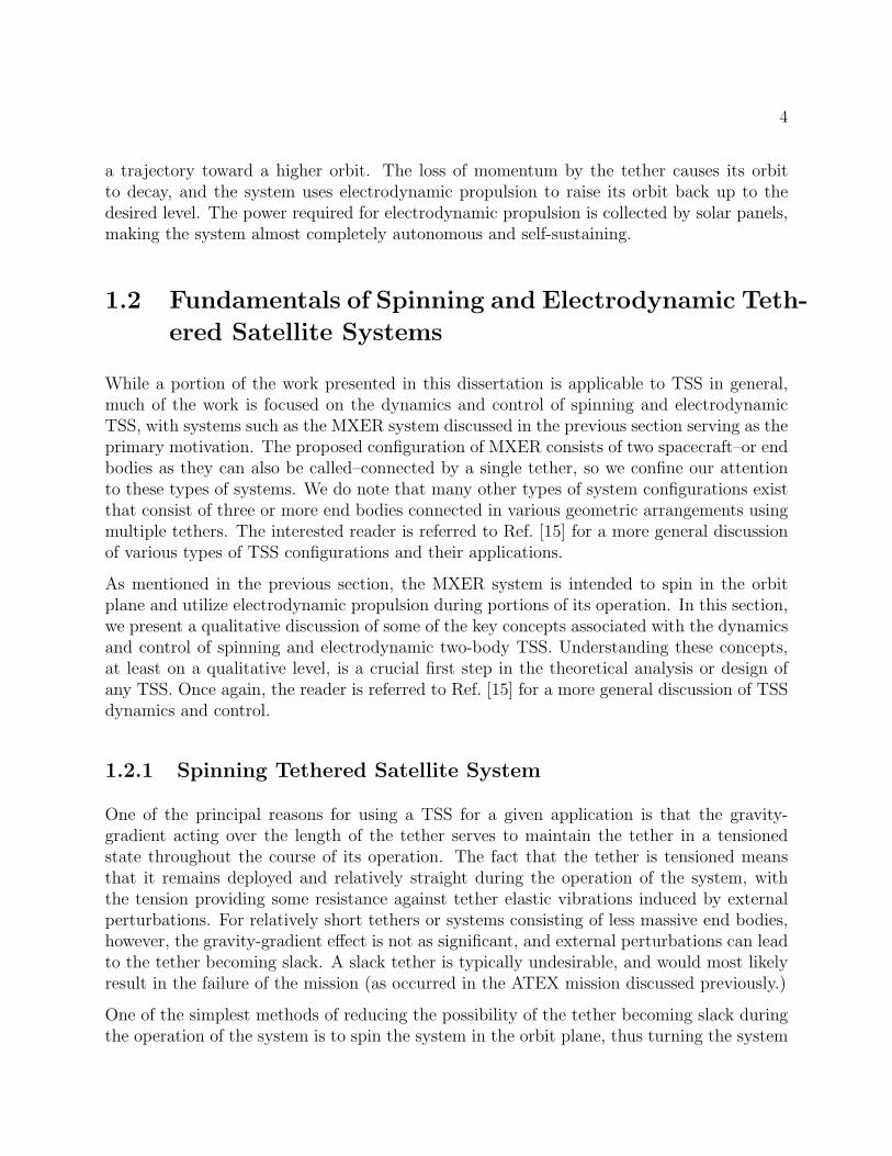
There are several aspects of the dynamics of a spinning TSS that can have a significantimpact on the operation of the system. Understanding these dynamics is a critical part ofthe design or analysis of any spinning TSS. The various aspects of the system dynamics areillustrated in Fig. 1.1, and include the orbital motion of the system, the motion of the tether,and the attitude motion of the end bodies.

The orbital motion of the system defines the state of some reference point in the systemrelative to the central body. The reference point is typically chosen as the system masscenter, or some convenient point on one of the end bodies. The orbital motion is affected bya number of different influences, including the gravity of the central body, the distributedmass of the system, and any external forces acting on the system such as atmospheric dragand electrodynamic forcing. The relative influence of each of these factors depends on thespecific spinning TSS and its operational regime.

The motion of the tether can be decomposed into two parts, as illustrated in Fig. 1.1. Thefirst part of the tether motion is a pendular mode that defines the motion of the line con-necting the ends of the tether. This pendular mode can be thought of as the attitude motionthat the tether would display if it were a rigid rod, and is affected by the mass propertiesof the system and the external forces acting on the system. For a typical spinning TSS, thependular motion is ideally a rotation in the orbit plane; however, external perturbations willresult in small out-of-plane deviations for the nominal planar motion. The pendular motionof the tether can therefore be viewed as a combination of an in-plane rotation and smallout-of-plane librations. The second component of the tether motion is the elastic vibrationsof the tether, which can be divided into transverse and longitudinal vibrations. The tether

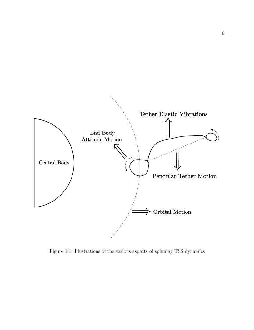
6

Central BodyCentral Body

=⇒=⇒

=⇒=⇒

=⇒=⇒

Orbital MotionOrbital Motion

Pendular Tether MotionPendular Tether Motion

Tether Elastic VibrationsTether Elastic Vibrations

End Body

Attitude Motion

End Body

Attitude Motion

=⇒=⇒

Figure 1.1: Illustrations of the various aspects of spinning TSS dynamics

7

elastic vibrations are affected by the external forces acting along the tether as well as thephysical and material properties of the tether. Note that the pendular motion and the elasticvibrations of the tether are coupled, in that neither is independent of the other.

The final component of the system dynamics is the attitude motion of the end bodies, which isdependent upon the inertia properties of the end bodies and driven by the external momentsacting on the end bodies. A component of the external moment acting on each end bodyis due to the tensions applied by any tethers attached to the body, so the attitude motionof the bodies is affected by the motion of the tether. Likewise, the motion of the tethers isaffected by the attitude motion of the end bodies, because motion of the end bodies affectsthe conditions at the ends of the tethers. Similarly, the orbital motion of the system affectsboth the tether motion and the attitude motion of the end bodies and vice versa, so all ofthe motions of a spinning TSS are coupled to one another. This coupling makes analyzingthe dynamics of a spinning TSS quite difficult, but also means that spinning TSS dynamicsare quite rich and interesting. One of the principle objectives of the work presented in thisdissertation is to analyze several of the key aspects of spinning TSS dynamics.

1.2.2 Electrodynamic Tethered Satellite System

The primary difference between an electrodynamic TSS and a conventional TSS is that thetether in an electrodynamic TSS is electrically conductive and intended to carry an electricalcurrent. The current in the conductive tether interacts with the magnetic field of the centralbody, resulting in a distributed force along the length of the tether. This force provides aform of propellantless propulsion for the system that can be used to affect all aspects of thesystem dynamics.

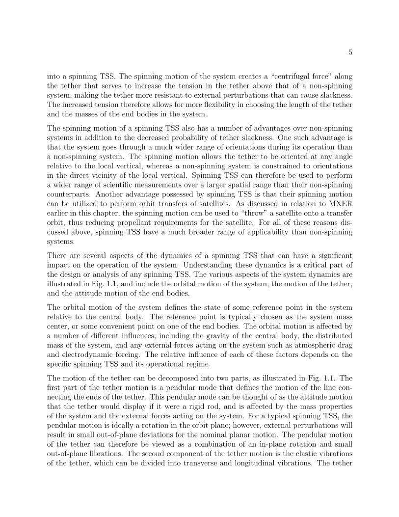
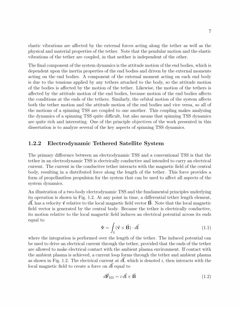
An illustration of a two-body electrodynamic TSS and the fundamental principles underlyingits operation is shown in Fig. 1.2. At any point in time, a differential tether length element,d~l, has a velocity ~v relative to the local magnetic field vector ~B. Note that the local magneticfield vector is generated by the central body. Because the tether is electrically conductive,its motion relative to the local magnetic field induces an electrical potential across its endsequal to

Φ =

∫L

(~v× ~B) · d~l (1.1)

where the integration is performed over the length of the tether. The induced potential canbe used to drive an electrical current through the tether, provided that the ends of the tetherare allowed to make electrical contact with the ambient plasma environment. If contact withthe ambient plasma is achieved, a current loop forms through the tether and ambient plasmaas shown in Fig. 1.2. The electrical current at d~l, which is denoted i, then interacts with thelocal magnetic field to create a force on d~l equal to

d~FED = i d~l× ~B (1.2)

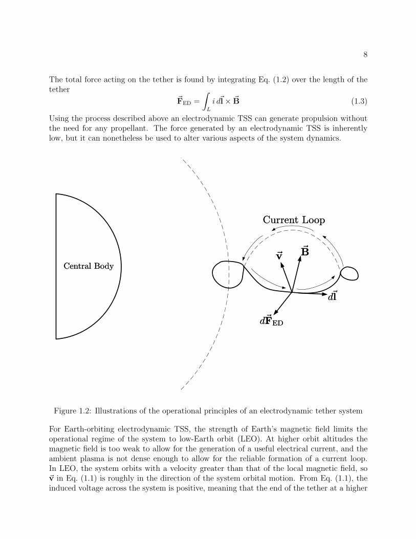
8

The total force acting on the tether is found by integrating Eq. (1.2) over the length of thetether

~FED =

∫L

i d~l× ~B (1.3)

Using the process described above an electrodynamic TSS can generate propulsion withoutthe need for any propellant. The force generated by an electrodynamic TSS is inherentlylow, but it can nonetheless be used to alter various aspects of the system dynamics.

Central BodyCentral Body

BB

dFEDdFED

Current LoopCurrent Loop

vv

dldl

Figure 1.2: Illustrations of the operational principles of an electrodynamic tether system

For Earth-orbiting electrodynamic TSS, the strength of Earth’s magnetic field limits theoperational regime of the system to low-Earth orbit (LEO). At higher orbit altitudes themagnetic field is too weak to allow for the generation of a useful electrical current, and theambient plasma is not dense enough to allow for the reliable formation of a current loop.In LEO, the system orbits with a velocity greater than that of the local magnetic field, so~v in Eq. (1.1) is roughly in the direction of the system orbital motion. From Eq. (1.1), theinduced voltage across the system is positive, meaning that the end of the tether at a higher

9

orbit altitude is at a higher electric potential than the end of the tether at a lower orbitaltitude. If a current loop is formed through the tether and ambient plasma, the current isnaturally driven in the direction shown in Fig. 1.2–from the lower end body to the upper endbody. According to Eq. (1.2), the electrodynamic force generated on the tether is thereforeacting in the direction opposite the orbital motion, and serves to decay the system orbit.However, no power is required to generate the current in the tether because it is driven bythe naturally induced voltage, and the current can therefore be used to charge a power sourceif one is placed in the current loop. Because of this fact, an electrodynamic TSS operatingas described above is said to be operating in the “generator mode.” In this operationalmode, electrical energy is gained in the form of a charged power source at the expense of themechanical energy of the system.

In addition to being charged if the system is operating in the generator mode, a power sourcecan be used to reverse the naturally occurring induced voltage such that the lower end body isat a higher electric potential than the upper end body. The electrical current therefore flowsfrom the upper end body to the lower end body, and the resulting electrodynamic force is inthe same direction as the system orbital motion. In this case the electrodynamic force servesas a thrust force that raises the system orbit, and an electrodynamic TSS operating in sucha manner is therefore said to be operating in the “thruster mode.” In this operational mode,the mechanical energy of the system is increased at the expense of electrical energy in theform of an applied power source. The discussion presented above applies to electrodynamicTSS orbiting bodies other than Earth; however, we must note that the generator and thrustermodes can be slightly different for systems orbiting other central bodies, and there can evenbe some overlap between the two modes. For example, the magnetic field of Jupiter is stillquite strong at altitudes above its synchronous altitude, so Jupiter-orbiting electrodynamicTSS can operate above the synchronous altitude. This means that the velocity of the systemrelative to the magnetic field is opposite the system motion, and a force in the directionof the system orbital motion can be generated using the naturally induced voltage. It istherefore possible for a Jupiter-orbiting electrodynamic TSS to generate a thrust force thatraises the system orbit while simultaneously charging a power source.

As with any TSS, the primary aspects of the dynamics of an electrodynamic TSS are thesystem orbital motion, the tether motion, and the attitude motion of the end bodies. Thecharacteristics of these aspects of the system dynamics are similar to those described for anspinning TSS in § 1.2.1. With an electrodynamic TSS, however, perhaps the most impor-tant aspect of the system dynamics is the effect of the electrodynamic force on the variouscomponents of the system motion.

The main effect of the electrodynamic force on the orbital motion of the system is to increaseor decrease the orbit radius, depending on whether the system is operating in the thruster orgenerator mode. The change in the orbit radius is slow due to the relatively low magnitudeof the electrodynamic force, but over long enough time scales significant changes in the orbitradius can be achieved. The electrodynamic force also changes the orientation in space ofthe system orbit, but these changes are much slower than the change in the orbit radius.

10

The electrodynamic force affects both the pendular and flexible modes of the tether motion.For local vertically aligned systems, the electrodynamic force drives both in- and out-of-plane librations of the system about the nominal alignment with the local vertical. Forspinning systems, the electrodynamic force can either increase or decrease the in-plane spinrate depending on the direction of the force, and also drives out-of-plane librations thatare deviations from the nominal planar spinning motion. Because the electrodynamic forceacts tangent to the tether, only the transverse elastic vibrations of the tether are directlyaffected by the electrodynamic force. However, the transverse vibrations are coupled to thelongitudinal vibrations of the tether, so the electrodynamic force affects all aspects of thetether elastic vibrations.

Th electrodynamic force only acts along the tether, so it does not directly affect the attitudemotion of the end bodies. As with a spinning TSS, however, the end body attitude motionin an electrodynamic TSS is affected by the tether motion and the system orbital motion,so the electrodynamic force has an indirect affect on the end body attitude motion.

From the discussions presented in this section it is evident that the dynamics of spinningand electrodynamic TSS can be quite complicated and rich. The analysis and design of anyTSS mission requires more than the qualitative insights discussed thus far, and the literaturecontains a vast amount of detailed analysis of various types of TSS. In the next section, wepresent a review of the most relevant studies related to the dynamics and control of spinningand electrodynamic TSS.

1.3 Review of Relevant Literature

Dating back to Tsiolkovsky, literally hundreds of studies of TSS dynamics and controlhave been published in the literature. Two excellent survey articles on the topic of non-electrodynamic TSS dynamics and control are those written by Misra and Modi,41 andKumar.30 The former article provides a survey of works published prior to 1986, while thelatter provides a survey of works published after 1986.

As mentioned previously, some of the work presented in this dissertation applies to TSS ingeneral, but we are mostly concerned with the dynamics and control of spinning and elec-trodynamic TSS, with systems such as the MXER system discussed in §1.1 are our primarymotivation. The proposed configuration of MXER consists of two spacecraft connected by asingle tether, so we confine our survey of the relevant literature to studies that have consid-ered these types of systems. In addition, we are specifically interested in the dynamics andcontrol of the system in its operational configuration, meaning that we are not concernedwith deployment or retrieval of the tether. We therefore also confine our review of the rele-vant literature to studies of systems in their operational configuration. We do point out thatin this section a more thorough review of the literature on electrodynamic TSS is presentedthan is presented for other systems. This is due to the fact that several survey articles on

11

non-electrodynamic TSS have been published in the past, while no such survey exists forelectrodynamic TSS. We hope that the literature review presented in this section may serveas a useful introduction to the dynamics and control issues associated with electrodynamicTSS.

1.3.1 Spinning Tethered Satellite Systems

The literature contains a large number of studies on the dynamics of spinning TSS datingback to the early years of human spaceflight. The earliest studies of spinning TSS dynamicswere motivated by their possible use for generation of artificial gravity in space. Tai andLoh63 studied the dynamics of a space-station connected to a counterweight by a flexiblecable. The spinning motion of the system was confined to the orbital plane, and numericalsimulations were used to analyze the system dynamics. Chobotov12 studied a spinningTSS by modeling the system as two point masses connected by a massless linear spring.The system mass center remained on an unperturbed circular orbit and the motion of thesystem was confined to the orbital plane. Numerical solutions were used to study the systemdynamics. Crist and Eisley16 studied a system similar to that studied by Chobotov, butincluded some effects due to orbital eccentricity. A Floquet analysis was used to study thestability properties of the planar motion of the system.

Stabekis and Bainum60 studied a spinning TSS consisting of two finite, rigid end bodiesconnected by an extensible, massless tether. As in previous studies, the system mass cen-ter was constrained to a circular orbit and the motion was restricted to the orbital plane.The nonlinear equations of motion were linearized about equilibrium configurations and theRouth-Hurwitz criterion was used to analyze the stability of the planar motion.

Three-dimensional motion of a spinning TSS was considered by Bainum and Evans2 using amodel similar to that used in Ref. [60]. However, gravity-gradient effects were not included inthe model, so the motion of the system was torque-free. Bainum and Evans3 later extendedtheir analysis to include the effects of the gravity-gradient torque acting on the system. Thenonlinear equations of motion were linearized about a nominal spin in the orbit plane, andpossible resonances were identified. Some resonances in the attitude motion of the end bodieswere demonstrated using numerical simulations, and all of the simulations indicated smallout-of-plane motion of the tether. A rigorous stability analysis was not performed, althoughFloquet theory was suggested.

Another study of the three-dimensional motion of a spinning TSS was conducted by DeCou.17

Several system configurations were considered, but all consisted of point masses connectedby massless, fixed-length tethers with the system mass center constrained to a circular orbit.The system was nominally spinning in a plane with an arbitrary orientation relative to theorbital frame. Expressions were derived for the accelerations of the end bodies due to thegravity-gradient, and these expressions were used to derive differential equations governingthe out-of-plane motion of the end masses and the deviation of the spin rate from a nominal

12

value. The differential equation governing the out-of-plane motion contained periodic, time-varying coefficients that were assumed to be negligible to simplify the analysis. The resultinglinear, constant-coefficient differential equation was solved, and the solution for the out-of-plane motion was a combination of various sinusoidal terms. These solutions assumed thatthere was no initial out-of-plane motion, such that the motion remains planar if the desiredspin plane is the orbital plane.

Breakwell and Janssens8 studied the transverse vibrations of a two-body spinning TSS byassuming that the tether is inextensible and that the elastic vibrations of the tether have noeffect on the attitude motion of the tether. The system was assumed to be spinning in theorbit plane at a rate equal to the orbital rate, and the stability of small transverse oscillationswas analyzed using Floquet theory. The transverse vibrations were found to be unstable forcertain configurations of the system mass distribution, and methods of selecting the massesof the end bodies that avoid the instabilities are presented.

A rather extensive study of spinning TSS dynamics can be found in the book by Beletskyand Levin.5 Massless and massive tethers are considered, but in all cases the system masscenter is constrained to an unperturbed circular orbit. The planar motion of systems withmassless tethers is completely characterized, and bounds are placed on the possible out-of-plane motion for non-planar systems. The planar motion of massive tethers is studiedby assuming that the tether is flexible, but the elastic vibrations of the tether do no affectthe pendular motion of the tether. The elastic vibrations are thus superimposed upon thependular motion of a rigid tether. In addition, the longitudinal vibrations of the tether areignored and only transverse vibrations are considered. A Floquet analysis is used to showthat the transverse vibrations are unstable for certain in-plane spin rates and system massproperties. The results of this analysis are an extension of those presented by Breakwell andJanssens,8 in that different in-plane spin rates are considered.

Somewhat surprisingly, the literature contains few studies on the control of two-body spin-ning TSS in their operational configuration. Most studies of the control of two-body spinningTSS relate to deployment and retrieval of the tether, which is not the focus of the work pre-sented in this dissertation. The interested reader is referred to Refs. [41] and [30] for moreinformation of these topics. Most modern studies of spinning TSS control focus on control-ling large formations of satellites, such as triangular or diamond-shaped configurations. Anexcellent reference for work on these types of systems is the book by Levin,34 in which thedynamics and control of various types of TSS is studied related to specific TSS missions.As mentioned previously, we are only concerned with two-body systems, so works related todifferent spinning TSS configurations are not discussed here.

1.3.2 Electrodynamic Tethered Satellite Systems

Research on electrodynamic TSS is a relatively new branch of TSS research, having onlybegun during the past several decades. In general, the research on the dynamics and control

13

of electrodynamic TSS can be divided into two main categories, each focusing on a particularaspect of the system dynamics. The first category deals with the change in the system orbitdue to the electrodynamic force, and how the force can be used to control the system orbit.The second category deals with the motion of the tether and how it is specifically affectedby the electrodynamic force.

Orbital Maneuvering

One of the first studies on the effect of the electrodynamic force on the system orbit wasconducted by Beletsky and Levin.5 In their work, Beletsky and Levin considered a two-body electrodynamic TSS consisting of point mass end bodies connected by a flexible tether.The magnetic field of the central body was modeled as a non-tilted, non-rotating dipole.Approximations of the average rates-of-change of the orbital inclination, right-ascension ofthe ascending node, and orbital parameter were derived and analyzed. The average changesin the inclination and right-ascension of the ascending node were found to be quite small,even over relatively long time spans. However, over similar time spans the variation of theorbit parameter was found to be significant, reaching approximately 50 km over 100 orbitsfor a typical system.

Tragessear and San64 developed a simple guidance scheme for the orbital motion of a two-body electrodynamic TSS consisting of two point mass end bodies connected by a rigidtether. The magnetic field of the central body was modeled as a non-tilted, non-rotatingdipole, and the electrodynamic force was assumed to have a negligible influence on thetether attitude motion. The system was therefore assumed to remain aligned with the localvertical throughout its motion such that the orbital motion of the system comprised the onlydegrees of freedom. The time-averaged Gauss variational equations were used to developguidance laws for the osculating orbit elements of the system mass center, with the variationof the electrodynamic force achieved by modulating the current in the tether. Numericalsimulations were used to demonstrate the performance of the guidance laws.

The results of Tragessear and San were extended by Williams66 to include the effects of thependular motion of the tether. Optimal control laws for the osculating orbit elements of thesystem mass center were developed using the current in the tether as the control input. Theperformance of the optimal control laws was demonstrated using numerical simulations andcompared to the results of Tragesser and San. In certain cases, the inclusion of the pendularmotion of the tether in the guidance scheme led to improved performance over the guidancescheme that did not include the pendular motion.

Another extension of the work of Tragesser and San was made by Sabey and Tragesser.54

The attitude dynamics of the tether were included in the system dynamics by assuming thatthe attitude was controlled about a nominal periodic trajectory, and a similar procedure asthat used in Ref. [64] was used to determine guidance laws for the osculating orbit elementsof the system mass center.

14

Lanoix et al.31 considered the orbital dynamics of a more complicated and physically realisticsystem model than the studies discussed previously. The system consisted of two point massend bodies connected by an axially extensible tether. The magnetic field of the central bodywas represented using the International Geomagnetic Reference Field model, which expressesthe field in terms of a spherical harmonic series. Aerodynamic and thermal effects on thedynamics of the tether were also considered in the system model, and numerical simulationswere used to analyze the orbital motion of the system.

A recent study of electrodynamic TSS orbital maneuvering was conducted by Stevens andWiesel.62 As in previous studies, the system was modeled as two point mass end bodiesconnected by a rigid tether. The magnetic field of the central body was modeled as anon-tilted, non-rotating dipole, and atmospheric drag was included in the tether dynamicsmodel. As in the studies of Tragesser and San and Sabey and Tragessear, the time-averagedGauss form of the variational equations for the osculating orbit elements of the system masscenter were considered and used to develop optimal control laws for the orbital motion ofthe system. The control laws presented were for maximum final altitude, maximum finalinclination change, and minimum time orbital maneuvers.

Tether Dynamics and Control

Previous studies of the tether dynamics of electrodynamic TSS have typically focused oneither the pendular motion of the system or the elastic vibrations of the tethers. Someof the earliest studies of the pendular motion of electrodynamic TSS were conducted byLevin33 and Beletsky and Levin.5 In these studies, the system consists of two point massend bodies connected by a flexible, massless tether, with the system mass center constrainedto an unperturbed circular orbit. The magnetic field of the central body is modeled as anon-tilted, non-rotating dipole and the orbit of the system was confined to the plane of themagnetic equator. The current in the tether is assumed constant throughout the motion.Because the tether is massless and the system orbit is in the magnetic equatorial plane, theshape of the tether can be determined at any moment in time such that the tether attitudeangles are the only degrees of freedom of the system. Equilibrium configurations for the tetherattitude angles are determined and their linear stability is analyzed. The stability analysisshows that the operational equilibrium configurations of a two-body electrodynamic TSSare always unstable under a constant current. The instabilities are attributed to a constantpumping of energy into the pendular motion of the tether by nonconservative componentsof the electrodynamic force.

The studies of Levin and Beletsky and Levin were extended to electrodynamic TSS systemson inclined circular orbits by Pelaez et al.47 In this study, the system consists of two pointmass end bodies connected by a massive, rigid tether, and the magnetic field of the centralbody is modeled as a non-tilted, non-rotating dipole. The current in the tether is once againassumed to be held constant. Unlike the previous studies, the circular orbit on which the

15

system mass center is constrained is allowed to have an inclination relative to the planeof the magnetic equator. As a result, the electrodynamic force varies periodically with aperiod equal to the orbital period, and equilibrium configurations for the tether attitudecan no longer be determined. However, periodic solutions are determined and their stabilityis analyzed using Floquet theory. As with systems confined to the magnetic equator, theperiodic solutions of two-body electrodynamic TSS on inclined orbits are always unstableunder the action of a constant current. The instabilities are once again attributed to aconstant pumping of energy into the system by the electrodynamic force.

Several further extensions of the work in Ref. [47] were performed to consider a much largerfamily of periodic tether attitude trajectories46 and systems on elliptical inclined orbits.45 Ineach of these studies the tether attitude motion was once again found to always be unstabledue to the same energy pumping mechanism discussed previously.

One of the earliest studies of the elastic vibrations of an electrodynamic TSS was conductedby Belestsky and Levin.5 In this study, the system consists of two point mass end bodiesconnected by a flexible, massive tether, with the system mass center constrained to a circularorbit. The magnetic field of the central body is modeled as a non-tilted, non-rotating dipoleand the system orbit is confined to the plane of the magnetic equator. Planar equilibriumconfigurations are determined for the case of constant current in the tether, and the linearstability of the equilibrium configurations is analyzed. As with the attitude motion of atwo-body electrodynamic TSS in the plane of the magnetic equator, the elastic vibrationsare always unstable under a constant current. The instability occurs in both the transverseand longitudinal vibrations due to the coupling between those two motions, and is once againattributed to energy pumping by the electrodynamic force.

The transverse vibrations of a two-body electrodynamic TSS on an inclined circular orbitwere considered by Pelaez et al.48 The magnetic field is modeled as a non-tilted, non-rotatingdipole and the current in the tether is held constant. The transverse vibrations of the tetherare modeled by assuming that the tether is comprised of two articulated rigid rods. Periodictrajectories for the system dynamics are determined and their linear stability is analyzednumerically. Two different system configurations are studied: one in which only a portion ofthe tether carries an electrical current; and another in which the entire length of the tethercarries an electrical current. For both types of systems, the periodic motions are found toalways be unstable.

Somenzi et al.59 studied the transverse vibrations of a two-body electrodynamic TSS con-sisting of two point mass end bodies connected by a flexible, but inextensible, tether. Thesystem mass center is constrained to a circular inclined orbit, and the magnetic field ismodeled using the International Geomagnetic Reference Field model. Some effects on thecurrent in the tether due to the ambient plasma environment and average solar activity arealso included in the dynamic model. The tether transverse vibrations are expanded in nor-mal modes, and the system equations of motion are linearized about an alignment with thelocal vertical. A linear stability analysis is performed considering only the first two modes

16

of the transverse vibrations, and shows that the system is always unstable.

The studies discussed above indicate that the tether dynamics of electrodynamic TSS areinherently unstable. As mentioned previously, the instability is due to a constant pumping ofenergy into the system by non-conservative components of the electrodynamic force. Becausethe pendular motion and elastic vibrations of the tether are coupled, any instability in oneaspect of the tether motion is transmitted to the other. The inherent instability in the tethermotion means that successful operation of any electrodynamic TSS requires some means ofcontrolling both the pendular motion and elastic vibrations of the tether.

Corsi and Iess14 considered the control of the pendular motion of an electrodynamic TSS forsatellite deorbiting applications. The system considered in the study consists of two pointmass end bodies connected by a rigid tether. A Lyapunov function is used to derive a controllaw that keeps the in- and out-of-plane motions of the tether within pre-defined bounds, andthe performance of the control law is demonstrated with numerical simulations. The controllaw is based on a simple on-off switching of the electrical current in the tether (and thus theelectrodynamic force) that is demonstrated to keeps the tether attitude motion bounded.

Libration control of a system model similar to that considered by Corsi and Iess was con-sidered by Pelaez and Lorenzini.25 The system is modeled as two point masses connectedby a rigid tether, and the system mass center is assumed to remain fixed on an inclinedcircular orbit. The latter assumption means that the influence of the electrodynamic forceon the orbital motion is considered negligible for the systems and time scales considered inthe study. The magnetic field of the central body is modeled as a non-tilted, non-rotatingdipole. Simple feedback control laws are derived that control the attitude motion of thetether about periodic trajectories for a constant current in the tether. The control of thetether attitude motion is achieved by adding “appropriate forces” into the system model, sono physical mechanism for providing the control inputs is given. Floquet theory is used todetermine stability boundaries that are related to the control gains used in the control laws,and numerical simulations are used to demonstrate the effectiveness of the control laws.

Williams67 also considered the control of the tether attitude motion about a periodic trajec-tory. The model considered by Williams is identical to that studied by Pelaez and Lorenzini.25

Control about the periodic trajectory is achieved by modulating the current in the tetherbased on feedback measurements of the system Hamiltonian relative to the Hamiltonian ofthe desired periodic trajectory. Stability boundaries are determined using Floquet theoryas functions of the control gain of the control law, and a numerical simulation is used todemonstrate the performance of the control law.

Zhou et al.71 developed control laws for the tether attitude motion by using the rate-of-change of the tether length as an additional control input. The system considered consistsof two point mass end bodies connected by a rigid tether, and the magnetic field is modeledas a non-tilted, non-rotating dipole. Feedback linearization is used to determine control lawsfor the tether current and rate-of-change of length that regulate the attitude motion aboutthe local vertical. Numerical simulations are used to demonstrate the performance of the

17

control laws.

A recent study by Williams69 considers the control of the tether attitude motion abouta periodic trajectory using what the author calls “time-delayed predictive control.” Thecontrol of the attitude motion is achieved using modulation of the current in the tether asthe only control input. The system is modeled as two point mass end bodies connectedby a rigid tether. Numerical simulations are used to demonstrate the performance of thecontroller for the case of the system constrained to a circular orbit about a central bodywith a non-tilted dipole magnetic field. Several numerical simulations are also performedfor systems in which the orbital variations due to the electrodynamic force are included inthe model, and the magnetic field is modeled as a tilted dipole that rotates with the centralbody. In these cases, the controller cannot drive the tether attitude motion exactly to thedesired periodic trajectory, but it does stabilize the attitude motion in the sense that theattitude motion remains bounded and “close” to the desired periodic trajectory for all time.

Equilibrium-to-equilibrium maneuvers of electrodynamic TSS are considered by Mankalaand Agrawal.35 The system model used in the study consists of two point mass end bodiesconnected by a rigid tether, with the system constrained to a circular orbit. The magneticfield of the central body is modeled as a non-tilted, non-rotating dipole and the motion of thesystem is confined to the plane of the magnetic equator. Equilibrium configurations for theplanar tether attitude angle are determined, and control laws for the current in the tetherare determined using feedback linearization. These control laws drive the system from oneequilibrium configuration to another, and their performance is demonstrated using numericalsimulations. Another study by Mankala and Agrawal36 considers equilibrium-to-equilibriummaneuvers of flexible electrodynamic TSS. The system model is identical to that used inRef. [35], with the exception that the tether is modeled as flexible, but massless. Onceagain, feedback linearization is used to derive control laws that drive the system from oneequilibrium configuration to another.

All of the studies of electrodynamic TSS control discussed to this point have only consideredcontrol of the pendular motion of the tether. However, several studies have also consideredcontrol of the elastic vibrations of the tether. Beletsky and Levin5 considered tether vibrationcontrol of a system consisting of two point mass end bodies connected by a flexible tether.Control laws based on modulations of the current in the tether were determined that regulatesmall tether elastic vibrations about a nominal equilibrium configurations. These control lawsare determined assuming that the magnetic field of the central body is a nontilted dipole,and that the motion of the system takes place entirely in the plane of the magnetic equator.

Hoyt22 develops two different feedback control laws for the elastic vibrations of a two-bodyelectrodynamic TSS. The first control method is based on measurements of the position ofthe tether at various points along its length. These measurements are made by beaconsthat must be attached to various points along the tether. The second control method doesnot require any knowledge of the tether motion, and only requires knowledge of the relativeacceleration of the end bodies. Numerical simulations are used to demonstrate that the

18

control laws are successful in stabilizing the tether elastic vibrations over relatively longtime spans.

Watanabe et al.65 use input shaping to control the elastic vibrations of a two-body electro-dynamic TSS. A lumped mass model in which the tether is modeled as a finite number ofpoint masses connected by springs is used to account for the flexibility of the tether. Themagnetic field is modeled as a non-tilted, non-rotating dipole and the system mass center isconstrained to a circular orbit in the plane of the magnetic equator. Numerical simulationsare used to demonstrate that the control method is successful in reducing the amplitude ofthe tether elastic vibrations relative to those seen in an uncontrolled system.

Control of a continuum tether model is considered by Williams et al.70 The electrodynamicTSS considered in this study is a two-body system with the system mass center constrainedto a circular orbit. The magnetic field of the central body is modeled as a non-tilted, non-rotating dipole. Control laws are developed for the tether transverse vibrations by assumingthat the transverse vibrations are governed by the linear, one-dimensional wave equation andapplying principles of wave-absorbing control design. The control is applied by movementof the tether attachment point at one of the end bodies. The transverse vibration controlis combined with a tether pendular control law to provide complete control of the tethermotion. The performance of the control is demonstrated using numerical simulations forstationkeeping, deployment, and retrieval of the tether.

1.3.3 Spinning Electrodynamic Tethered Satellite Systems

A number of studies contained in the literature consider two-body TSS that are both spin-ning and utilizing electrodynamic propulsion. Pearson et al.44 proposed using spinningelectrodynamic TSS for orbital maneuvering and showed that they can generally providemuch greater performance than local-vertical aligned systems. Several minimum-time or-bit maneuvers utilizing spinning electrodynamic TSS were also computed and demonstratednumerically.

Williams68 studied spinning electrodynamic TSS orbital maneuvering by considering a sys-tem consisting of two point mass end bodies connected by a rigid tether. The magnetic fieldof the central body was modeled as a non-tilted, non-rotating dipole, and the entire systemwas assumed to spin at a constant rate in the orbital plane. This last assumption means thatthe effects of the electrodynamic force on the attitude dynamics of the tether are neglected.The methods used by Tragesser and San are used to develop guidance laws for the systemorbital motion, and numerical simulations are used to demonstrate the performance of theguidance laws. As done by Pearson et al., Williams concluded that spinning electrodynamicTSS are generally more effective orbit transfer vehicles than vertically aligned systems.

A relatively detailed study of the dynamics and control of two-body spinning electrodynamicTSS is contained in the book by Levin.34 In this work, the system is modeled as two point

19

mass end bodies connected by a massive, flexible tether. The basic operation of the systemis analyzed by determining how the electrodynamic force varies as the system spins, andhow the current in the tether can be modulated to produce a net force in a desired direction.The evolution of the spin rate and axis of the system due to the electrodynamic force andgravity-gradient torque is also considered. Levin finds that an appropriate modulation ofthe current in the tether can eliminate any average effects that the electrodynamic force hason the system spin rate, and the spin axis is only affected by the gravity-gradient torque ifthe spin plane is not the same as the orbit plane.

Small transverse vibrations of the tether in the two-body spinning electrodynamic TSS arealso considered by Levin. The rotation of the system is assumed uniform in this study,and the effects of the gravity-gradient are neglected. The primary result of the study is thatspinning electrodynamic TSS are preferable to vertically aligned electrodynamic TSS becausethey can operate at higher thrust levels due to the fact that the tether is in a higher stateof tension. Because the tether is at a higher tension, it is more resistant to external forces,and can thus be exposed to larger magnitude electrodynamic forcing without “inducing anycatastrophic dynamic responses.”

The final area of two-body spinning electrodynamic TSS dynamics and control consideredby Levin is that of orbital maneuvering. A current scheduling procedure is introduced thatallows for maximum orbit boost, orbit de-boost, and rotation of the orbit plane. Methodsof performing the fastest possible in-plane orbit transfers and orbit plane changes are alsoanalyzed.

1.4 Contributions of the Present Study

Although a great deal of research has already been conducted on the dynamics and controlof spinning and electrodynamic TSS, including numerous studies on spinning and electrody-namic TSS, there exist a number of topics that remain to be addressed. The purpose of thisdissertation is to address several of these open areas of study, and in this section we presentan overview of the original contributions made by this work.

1.4.1 Validation of Computational Models

In the literature review presented in the previous section a fair amount of attention was paidto the various modeling assumptions used to analyze the given TSS. Any TSS is a fairlycomplicated physical system, and as the literature review shows, it is common practice touse greatly simplified system models to study the dynamics and control of the system. Themathematical models associated with these simplified models are often relatively simple,and in many cases lend themselves to a rigorous analytical treatment. This practice of usingsimplified models is entirely justifiable, because the analysis of a system model that takes

20

into account every conceivable aspect affecting the system dynamics would be completelyintractable, even using numerical analysis techniques. However, the validity and practicalapplicability of results obtained using simplified system models should not be taken forgranted. It is entirely possible that the assumptions implicit in the simplified models removecritical aspects affecting the behavior of the system such that the predictions made by thesemodels have no resemblance whatsoever to the behavior of the actual physical system.

In an ideal situation, results obtained using simplified system models would be compared toexperimental data to test their validity. If the results compare favorably to the experimentaldata according to some objective metric, then the results are said to be validated. Theexperimental data used in the validation process is typically only available for a small subsetof the intended operational regime of the actual physical system, and the validated resultsobtained from the simplified system model are used to make predictions about the behaviorof the system for cases in which experimental data is not available. This type of processis commonly used in fields such as fluid and solid mechanics in which experimental data isreadily available.

Unfortunately, the above described process cannot be applied to results obtained related toTSS dynamics and control because experimental data is virtually nonexistent. This meansthat no results can be truly validated at the current point in time; however, it does notmean that some form of validation cannot be performed. In this dissertation we propose amethod of validating results obtained from simplified system models when experimental datais not available, as in the case of a TSS. The validation procedure requires the constructionof what we term a “top-level system model,” and an associated “top-level computationalmodel.” The top-level system model is a model of the system containing as few simplifyingassumptions as possible. It is intended that this model capture all of the relevant behaviors ofthe system, but can still be analyzed in a practical way. The top-level computational modelcontains all of the tools used to make predictions about the behavior of the system using thetop-level system model. Because of the complicated nature of the top-level system model,the predictions made by the top-level computational model are in the form of numericalsolutions which take the place of experimental data. All results obtained using simplifiedsystem models are compared to the predictions made by the top-level computational modelas a means of validation. If the results do not compare favorably, then the simplified systemmodel must be altered in some way so that it compares more favorably to the predictions ofthe top-level computational model.

In addition to the proposed computational model validation procedure, one of the majorcontributions of this work is the development of a top-level computational model that canbe used to perform validation of results obtained using simplified system models. This modelis developed with spinning and electrodynamic TSS specifically in mind; however, the modelcan be applied to a variety of other types of TSS as well. Most likely because of the lack ofexperimental data, validation of results obtained using simplified system models is seldom,if ever, performed in the field of TSS dynamics and control. It is the hope of the author thatthe validation method proposed in this work, combined with the availability of the top-level

21

computational model presented in this work, makes it much easier for other researchers tovalidate their results and better gage their practical applicability.

1.4.2 Verification of Computational Models

Because the numerical solutions produced by the top-level computational model act in placeof experimental data in the validation method we propose, the accuracy of the computercodes written to produce the numerical solutions must be rigorously verified. Errors in thesecodes, no matter how small, will lead to inaccurate numerical solutions that can be used tomake false claims about the validity of a result obtained from a simplified system model. Themethod we use in this work to verify the computer codes written for the top-level computa-tional model is the method of manufactured solutions, which is more commonly used in thefields of fluid and solid mechanics. To the author’s knowledge, this work constitutes the firstinstance in which the method of manufactured solutions is used to verify the computationalmodel of a TSS. We believe that the work presented herein demonstrates the relative easewith which the method is applied to a TSS, and we hope that this work encourages otherresearchers in the field of TSS dynamics and control to apply the method to their workwhenever applicable. Verification of computational models is another practice that is un-common in TSS dynamics and control research, and we believe that this work demonstratesits necessity.

1.4.3 Dynamics of Spinning Tethered Satellite Systems

As discussed in §1.3.1, most of the previous research on the dynamics of spinning TSS hasused simplified system models in which the out-of-plane pendular motion of the tether isneglected. A typical spinning TSS nominally spins in the orbit plane, so it is reasonable toneglect the out-of-plane motion in a preliminary study of spinning TSS dynamics; however,a complete picture of spinning TSS dynamics requires a rigorous analysis of the out-of-planependular motion of the system. Such an analysis is one of the main contributions of thiswork. A simplified system model is used to study the stability of small out-of-plane pendularmotion of the tether, and to determine approximate solutions for stable out-of-plane pendularmotion. These results obtained using a simplified system model are validated using numericalsolutions determined using the top-level computational model.

The transverse vibrations of the tether in a spinning TSS are also studied using a simplifiedsystem model, and conditions for unstable transverse vibrations are determined. Theseresults on the stability of spinning TSS transverse vibrations are not an original contribution,as they duplicate results obtained in Refs. [5] and [8]. The original contribution made inthis work is the application of the model validation procedure to these results. We use theprocedure to show that the instabilities predicted by the simplified system model are notpredicted by the top-level computational model, meaning that the results obtained using

22

the simplified model cannot be used to make predictions about an actual spinning TSS.We also present an analysis of the reasons behind the lack of agreement with the top-levelcomputational model, and propose ways in which the simplified system model can be changedto yield better agreement with the top-level computational model.

1.4.4 Control of Spinning Tethered Satellite Systems

In addition to the thorough analysis of the pendular motion of the tether in a spinningTSS, we also consider several methods of controlling the pendular motion. As discussed inthe literature review in §1.3.1, the literature contains surprisingly few studies on control ofspinning TSS, most likely because all TSS that have flown to date have been local-verticallyaligned systems. The control analysis presented in this work therefore constitutes an originalcontribution to the field of spinning TSS dynamics and control. A simplified system modelis used along with several nonlinear control design techniques to derive control laws thatallow the pendular motion of the tether to track a desired planar reference motion. Two ofthe control laws we develop are based upon principles of sliding mode control, which allowfor tracking of a reference trajectory in the presence of unmodeled dynamics (which arecertainly present for a simplified system model). Several of the control laws are applied tothe top-level computational model to assess their effectiveness and feasibility when appliedto a more physically realistic system model.

1.5 Organization of the Dissertation

The remainder of this dissertation is organized as follows. In Ch. 2, we present some funda-mental concepts of system modeling, along with the validation procedure that we propose foruse on systems for which experimental data is not available. The top-level system model usedin the validation procedure is presented in Ch. 3. All aspects of the top-level system modelare thoroughly developed, and several examples of the output of the top-level computationalmodel are presented. A detailed dynamic analysis of the motion of the tether in a spinningTSS is presented in Ch. 4. The analysis makes use of a lower-level system model so that anumber of analytical results pertaining to both the pendular motion and elastic vibrationsof the tether can be determined. All of these results are compared to numerical solutionsobtained using the top-level computational model to assess their applicability to an actualTSS. In Ch. 5, various methods of controlling the pendular motion of the tether in a spinningTSS are investigated, including the possibility of controlling the pendular motion using onlyelectrodynamic forcing. The control law developments in Ch. 5 make use of a lower-levelcomputational model, although several of the control laws take into account the effects ofunmodeled dynamics. Several of the control laws are applied to the top-level computationalmodel to assess their performance on a more realistic system model. Concluding remarksand recommendations for future work are offered in Ch. 6.

Chapter 2

Validation of Computational Models

In this chapter we present a procedure for validating the predictions made by computationalmodels when experimental data is not available, as in the case of a TSS. Many of the conceptsand much of the terminology presented in this chapter are adapted from the material inRefs. [43] and [51]. We first present some fundamental concepts related to modeling ofphysical systems and model validation as motivation for the development of the procedure.The validation procedure is then outlined in detail, and we discuss how it is applied tothe work related to the dynamics and control of TSS presented in the remainder of thisdissertation.

2.1 Fundamental Concepts of System Modeling

The first step in the analysis of any physical system is the careful and thoughtful developmentof a system model. The system model is the vehicle through which an actual physical systemis represented by a form that is suitable for scientific and engineering analysis. The wise andcareful development of the system model can result in the gain of a great deal of insight intothe behavior of the physical system, while a poor or uninformed development of a systemmodel can lead to incorrect predictions and erroneous results.

The various aspects of any system model can be arranged in the hierarchy shown in Fig. 2.1.At the top of the hierarchy sits the actual physical system that is being considered. Thephysical system consists of real components and hardware operating in a real physical envi-ronment. As an example, the work presented in this dissertation is focused on the dynamicsand control of spinning and electrodynamic TSS, so the physical system for any systemmodel we consider could be MXER, or any other similar TSS. Below the physical systemin the hierarchy are the three elements that make up the system model: 1) the conceptualmodel; 2) the mathematical model; and 3) the computational model. The objective of devel-oping the system model is to produce accurate predictions about the behavior of the actual

23

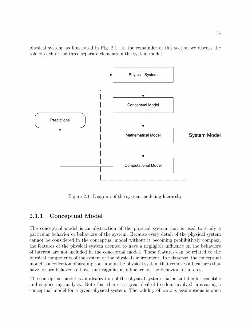
24

physical system, as illustrated in Fig. 2.1. In the remainder of this section we discuss therole of each of the three separate elements in the system model.

Physical System

Conceptual Model

Mathematical Model

Computational Model

Predictions

System Model

Figure 2.1: Diagram of the system modeling hierarchy

2.1.1 Conceptual Model

The conceptual model is an abstraction of the physical system that is used to study aparticular behavior or behaviors of the system. Because every detail of the physical systemcannot be considered in the conceptual model without it becoming prohibitively complex,the features of the physical system deemed to have a negligible influence on the behaviorsof interest are not included in the conceptual model. These features can be related to thephysical components of the system or the physical environment. In this sense, the conceptualmodel is a collection of assumptions about the physical system that removes all features thathave, or are believed to have, an insignificant influence on the behaviors of interest.

The conceptual model is an idealization of the physical system that is suitable for scientificand engineering analysis. Note that there is a great deal of freedom involved in creating aconceptual model for a given physical system. The validity of various assumptions is open

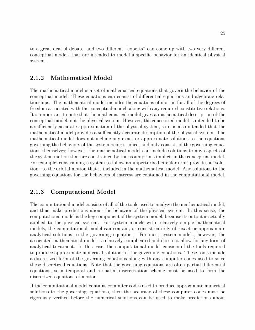
25

to a great deal of debate, and two different “experts” can come up with two very differentconceptual models that are intended to model a specific behavior for an identical physicalsystem.

2.1.2 Mathematical Model

The mathematical model is a set of mathematical equations that govern the behavior of theconceptual model. These equations can consist of differential equations and algebraic rela-tionships. The mathematical model includes the equations of motion for all of the degrees offreedom associated with the conceptual model, along with any required constitutive relations.It is important to note that the mathematical model gives a mathematical description of theconceptual model, not the physical system. However, the conceptual model is intended to bea sufficiently accurate approximation of the physical system, so it is also intended that themathematical model provides a sufficiently accurate description of the physical system. Themathematical model does not include any exact or approximate solutions to the equationsgoverning the behaviors of the system being studied, and only consists of the governing equa-tions themselves; however, the mathematical model can include solutions to any aspects ofthe system motion that are constrained by the assumptions implicit in the conceptual model.For example, constraining a system to follow an unperturbed circular orbit provides a “solu-tion” to the orbital motion that is included in the mathematical model. Any solutions to thegoverning equations for the behaviors of interest are contained in the computational model.

2.1.3 Computational Model

The computational model consists of all of the tools used to analyze the mathematical model,and thus make predictions about the behavior of the physical system. In this sense, thecomputational model is the key component of the system model, because its output is actuallyapplied to the physical system. For system models with relatively simple mathematicalmodels, the computational model can contain, or consist entirely of, exact or approximateanalytical solutions to the governing equations. For most system models, however, theassociated mathematical model is relatively complicated and does not allow for any form ofanalytical treatment. In this case, the computational model consists of the tools requiredto produce approximate numerical solutions of the governing equations. These tools includea discretized form of the governing equations along with any computer codes used to solvethese discretized equations. Note that the governing equations are often partial differentialequations, so a temporal and a spatial discretization scheme must be used to form thediscretized equations of motion.

If the computational model contains computer codes used to produce approximate numericalsolutions to the governing equations, then the accuracy of these computer codes must berigorously verified before the numerical solutions can be used to make predictions about

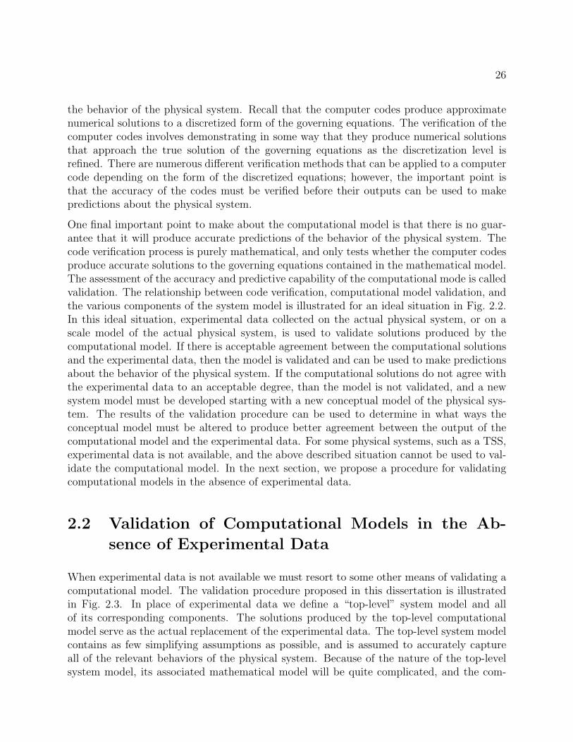
26

the behavior of the physical system. Recall that the computer codes produce approximatenumerical solutions to a discretized form of the governing equations. The verification of thecomputer codes involves demonstrating in some way that they produce numerical solutionsthat approach the true solution of the governing equations as the discretization level isrefined. There are numerous different verification methods that can be applied to a computercode depending on the form of the discretized equations; however, the important point isthat the accuracy of the codes must be verified before their outputs can be used to makepredictions about the physical system.

One final important point to make about the computational model is that there is no guar-antee that it will produce accurate predictions of the behavior of the physical system. Thecode verification process is purely mathematical, and only tests whether the computer codesproduce accurate solutions to the governing equations contained in the mathematical model.The assessment of the accuracy and predictive capability of the computational mode is calledvalidation. The relationship between code verification, computational model validation, andthe various components of the system model is illustrated for an ideal situation in Fig. 2.2.In this ideal situation, experimental data collected on the actual physical system, or on ascale model of the actual physical system, is used to validate solutions produced by thecomputational model. If there is acceptable agreement between the computational solutionsand the experimental data, then the model is validated and can be used to make predictionsabout the behavior of the physical system. If the computational solutions do not agree withthe experimental data to an acceptable degree, than the model is not validated, and a newsystem model must be developed starting with a new conceptual model of the physical sys-tem. The results of the validation procedure can be used to determine in what ways theconceptual model must be altered to produce better agreement between the output of thecomputational model and the experimental data. For some physical systems, such as a TSS,experimental data is not available, and the above described situation cannot be used to val-idate the computational model. In the next section, we propose a procedure for validatingcomputational models in the absence of experimental data.

2.2 Validation of Computational Models in the Ab-

sence of Experimental Data

When experimental data is not available we must resort to some other means of validating acomputational model. The validation procedure proposed in this dissertation is illustratedin Fig. 2.3. In place of experimental data we define a “top-level” system model and allof its corresponding components. The solutions produced by the top-level computationalmodel serve as the actual replacement of the experimental data. The top-level system modelcontains as few simplifying assumptions as possible, and is assumed to accurately captureall of the relevant behaviors of the physical system. Because of the nature of the top-levelsystem model, its associated mathematical model will be quite complicated, and the com-

27

Conceptual

Model

Mathematical

Model

Computational

Model

Physical

System

Computational

Solutions

Experimental

Data

Verification

Validation

Agreement

Predictions

Revise System

Model

YES

NO

Figure 2.2: Diagram illustrating the ideal situation for computational model validation

28

putational model consists entirely of tools used to generate approximate numerical solutionsof the mathematical model. It is important to note at this point that the top-level systemmodel cannot be so complicated as to render the generation of numerical solutions using thecomputational model impractical. These numerical solutions serve as the replacement forexperimental data, so it is imperative that they can be generated in a reasonable amount oftime. We must also note that the computer codes used to generate the numerical solutionsfor the top-level computational model must be rigorously verified. Because these solutionsserve as the basis for validation tests, there can be no doubt that they are accurate solutionsof the top-level mathematical model.

The complicated nature of the top-level system model makes it necessary to develop other,less complicated, system models. As shown in Fig. 2.3, we call these simplified system models“lower-level” system models. Any lower-level system model can be viewed as a simplificationof the top-level system model in that the lower-level model is developed using assumptionsin addition to those used to develop the top-level model. Note that all of the assumptionsused to develop the top-level system model must also be used to develop the lower-levelsystem model. The primary reason for developing a lower-level system model is that thesimplified nature of the lower-level model makes analysis using its computational modelmuch easier and more practical than analysis using the top-level computational model. Infact, the lower-level computational model may contain analytical solutions that can be usedto make predictions about the behavior of the physical system for the entire range of systemphysical parameters. In any case, being able to make predictions about the behavior of thephysical system using a lower-level system model is almost always preferable to using thetop-level system model due to the relative simplicity and ease of analysis using the former.Most of the previous research on TSS dynamics and control presented in §1.3 is based onthe analysis of lower-level computational models.

Because they are based on simplified system models, the results obtained from any lower-level computational model may or may not be applicable to the actual physical system. Inthe absence of experimental data, the applicability of these results is tested by comparingthem to numerical solutions generated using the top-level computational model. If thepredictions made by the two computational models are in acceptable agreement, then weconsider the lower-level computational model validated and its predictions can be appliedto the actual physical system. If the predictions made by the two computational modelsare not in acceptable agreement, then the lower-level computational model is not validated.In this case, we must use the results of the validation test to alter the lower-level systemmodel such that the predictions made by its computational model are in better agreementwith those made by the top-level computational model. This process is repeated until thetwo models are in sufficient agreement, at which point the lower-level computational modelis validated and can be used to make predictions about the actual physical system.

At this point we must stress the relative importance of the top-level system model in thevalidation procedure that we propose. The fundamental idea underlying the use of thetop-level system model in place of experimental data is that it is a sufficiently accurate

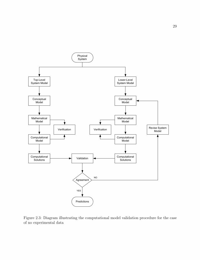
29

Conceptual

Model

Mathematical

Model

Computational

Model

Physical

System

Computational

Solutions

Verification

Validation

Agreement

Predictions

Revise System

Model

YES

NO

Lower-Level

System Model

Top-Level

System Model

Conceptual

Model

Mathematical

Model

Computational

Model

Verification

Computational

Solutions

Figure 2.3: Diagram illustrating the computational model validation procedure for the caseof no experimental data

30

representation of the actual physical system. A poor choice of the top-level system modeltherefore throws off the entire process, and makes any conclusions related to the validity oflower-level computational models practically meaningless. This is one of the main weaknessesof the proposed validation procedure. Another weakness of the procedure is that there isno way to test the validity of the top-level system model. Even a fairly complicated top-level model may not capture all of the relevant behaviors of the actual physical system,and there is no way to determine whether this is the case because there is no experimentaldata available with which to validate the top-level computational model. Despite theseweaknesses, we believe that the validation procedure proposed in this chapter is the bestway of performing some means of validation on results obtained from simplified systemmodels when experimental data is unavailable.

2.3 Application of the Proposed Validation Procedure

In the remaining chapters of this dissertation, the validation procedure proposed in thischapter is applied to various problems related to TSS dynamics and control. The top-levelsystem model and all of its components are developed in Ch. 3, in which we also verifythe accuracy of the computer codes used to produce the numerical solutions for the top-level computational model. In Chs. 4 and 5, we derive a number of results related to TSSdynamics and control using lower-level system models. The validity of all of these results isexamined by applying the validation procedure presented in this chapter.

Chapter 3

Top-Level System Model

In this chapter we present the various components of the top-level system model used inthis work to study the dynamics and control of spinning and electrodynamic TSS. Themodeling assumptions that comprise the conceptual model are presented and discussed, andthe mathematical model that describes the system dynamics is derived. The mathematicalmodel contains partial differential equations that govern the elastic vibrations of the tether,and two different computational models based on different methods of spatially discretizingthese partial differential equations are developed. The first computational model is basedon the assumed modes method, and the second is based on the finite element method. Themethod of manufactured solutions is used to verify both of the computational models, and thetwo models are compared to determine which is better suited to spinning and electrodynamicTSS dynamics and control applications. We conclude the chapter by presenting two examplesof the output generated by the top-level computational model: 1) an example for a spinningTSS; and 2) an example for an electrodynamic TSS1.

3.1 Physical System and Conceptual Model

The physical system under consideration is a TSS in orbit around an arbitrary central body.The system consists of two end bodies connected by a single tether. The central body hasa magnetic field, and the tether is conductive and capable of producing and electrodynamicforce.

Several modeling assumptions are made related to the physical environment of the system.We first assume that the central body is spherical with a homogeneous mass distribution,and therefore acts as a point mass. By making this assumption we are assuming thatthe Newtonian component of the gravitational field of the central body is the dominant

1The material presented in this chapter is also presented in Ref. [18].

31

32

component, and all of the higher-order components of the field due to the non-sphericalshape and non-uniform mass distribution of the central body have a negligible influence onthe system dynamics. We next assume that the magnetic field of the central body is a tilteddipole that is centered at the center of the central body and fixed to the central body asit rotates. This assumption means that we are considering any higher-order harmonics ofthe magnetic field of the central body to be negligible relative to its dipole component. Thefinal environmental assumption we make is that the gravitational force of the central bodyand the electrodynamic force acting on the tether are the only external forces acting on thesystem. By making this assumption, we are assuming that all other external forces otherthan the gravity of the central body and the electrodynamic force, such as atmospheric dragand solar radiation pressure, have a negligible influence on the system dynamics.

The modeling assumptions related to the actual TSS are as follows. Both of the end bodiesin the system are treated as finite rigid bodies, meaning that any elastic vibrations that theyundergo during operation are considered negligible. Because the tether in a typical TSS islong and thin, we model the tether as an elastic string that can only resist axial stretching.This assumption implies that the tether cannon support any amount of compression, andhas negligible bending and torsional stiffness.

3.2 Mathematical Model

Using the modeling assumptions outlined above we develop the mathematical model for thedynamics of the top-level system model. A diagram of the system is shown in Fig. 3.1. Theend bodies are denoted A and B, where A is the primary end body and B is the secondaryend body. The mass centers of A and B are denoted GA and GB, respectively. The tetherattaches to A at the point PA, and attaches to B at the point PB. The center of the centralbody is denoted O, which is taken as an inertial point.

Because A is the primary end body, the state of A is used to represent the orbital motion ofthe system. The state of A is parameterized using a set of osculating classical orbit elements

e =(a e Ω I ω ν

)T(3.1)

where a is semimajor axis, e is eccentricity, Ω is right-ascension of the ascending node(RAAN), I is inclination, ω is argument of periapsis, and ν is true anomaly. At any momentin time, e defines an instantaneous Keplerian orbit, known as the osculating orbit, that canbe used to determine the position and velocity of GA relative to O. Let ~rA be the position ofGA relative to O. The position of PA relative to GA is denoted ~pA. Let ds be a differentialtether length element located at an arclength s along the tether measured from PA, and let~r be the position of ds relative to PA. The position of PB relative to GB is denoted ~pB.

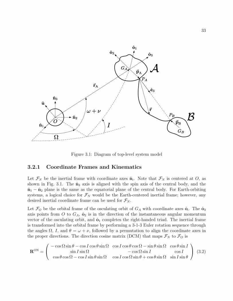
33

ΩΩ

II

ω + νω + ν

n1n1

n2n2

n3n3

o1o1o2o2 o3o3

e3e3

rr

AA

BBOO

uu

GAGA

PAPA

PBPB

GBGB

pApA

pBpB

rArA

Figure 3.1: Diagram of top-level system model

3.2.1 Coordinate Frames and Kinematics

Let FN be the inertial frame with coordinate axes ni. Note that FN is centered at O, asshown in Fig. 3.1. The n3 axis is aligned with the spin axis of the central body, and then1 − n2 plane is the same as the equatorial plane of the central body. For Earth-orbitingsystems, a logical choice for FN would be the Earth-centered inertial frame; however, anydesired inertial coordinate frame can be used for FN .

Let FO be the orbital frame of the osculating orbit of GA with coordinate axes oi. The o3

axis points from O to GA, o2 is in the direction of the instantaneous angular momentumvector of the osculating orbit, and o1 completes the right-handed triad. The inertial frameis transformed into the orbital frame by performing a 3-1-3 Euler rotation sequence throughthe angles Ω, I, and θ = ω + ν, followed by a permutation to align the coordinate axes inthe proper directions. The direction cosine matrix (DCM) that maps FN to FO is

RON =

− cos Ω sin θ − cos I cos θ sin Ω cos I cos θ cos Ω− sin θ sin Ω cos θ sin Isin I sin Ω − cos Ω sin I cos I

cos θ cos Ω− cos I sin θ sin Ω cos I cos Ω sin θ + cos θ sin Ω sin I sin θ

(3.2)

34

The angular velocity and acceleration of FO relative to FN are

~ωO/N =

√µp

r2A

o2

= θo2

(3.3)

~ωO/N = −2µe sin ν

r3A

o2

= θo2

(3.4)

where µ is the gravitational parameter of the central body, and the quantities p and rA aredefined as

p = a(1− e2) (3.5)

rA =p

1 + e cos ν(3.6)

Note that p is the orbital parameter of the osculating orbit, and rA is the instantaneous orbitradius of GA.

Let FA be a body-fixed principal coordinate frame for A, with coordinate axes ai. Similarly,let FB be a body-fixed principal coordinate frame for B, with coordinate axes bi. Theorientations of FA and FB relative to FO are defined using the quaternions

qA =(qA1 qA2 qA3 qA4

)T

=(

qTA qA4

)T(3.7)

qB =(qB1 qB2 qB3 qB4

)T

=(

qTB qB4

)T(3.8)

Note that a quaternion is defined as

q =(

qT q4

)T(3.9)

q = a sin

(Φ

2

)(3.10)

q4 = cos

(Φ

2

)(3.11)

where a contains the components of the unit principal rotation axis and Φ is the principalrotation angle. We choose a quaternion to parameterize the orientation of both FA and FBrelative to FO because we want the mathematical model to be valid for arbitrary attitude mo-tion of the end bodies. Because a quaternion is a nonsingular attitude parameterization, wedo not have to place any bounds on the end body attitude motion to avoid the mathematicalsingularities associated with singular attitude parameterizations, such as Euler angles.

35

The DCM for a general quaternion is

R = (q24 − qTq)1 + 2qqT − 2q4q

× (3.12)

where 1 is the identity matrix and

q× =

0 −q3 q2

q3 0 −q1

−q2 −q1 0

(3.13)

The DCMs that map FO to FA and FO to FB are therefore

RAO = (q2A4 − qT

AqA)1 + 2qAqTA − 2qA4q

×A (3.14)

RBO = (q2B4 − qT

BqB)1 + 2qBqTB − 2qB4q

×B (3.15)

respectively. Let ~ωA/O be the angular velocity of FA relative to FO, and let ωA/O contain thecomponents of ~ωA/O expressed relative to FA. Similarly, let ~ωB/O be the angular velocity ofFB relative to FO, and let ωB/O contain the components of ~ωB/O expressed relative to FB.The time derivatives of qA and qB can then be expressed as

˙qA =1

2B(qA)ωA/O (3.16)

˙qB =1

2B(qB)ωB/O (3.17)

where

B(q) =

[q× + q41−qT

](3.18)

Let FE be a tether-fixed coordinate frame with coordinate axes ei. The orbital frame istransformed to FE by performing a 2-1 Euler rotation sequence through the angles α and−β, as shown in Fig. 3.2. The DCM that maps FO to FE is

REO =

cosα 0 − sinα− sinα sin β cos β − cosα sin βsinα cos β sin β cosα cos β

(3.19)

and the angular velocity of FE relative to FO is

~ωE/O = βe1 + α cos βe2 + α sin βe3 (3.20)

The axis e3 points from PA to PB such that FE defines the orientation of the undeformedtether line relative to FO. The angles α and β can therefore be viewed as the in- and out-of-plane attitude angles of the tether relative to FO. The evolution of α and β over timedefines the pendular mode of the tether motion.

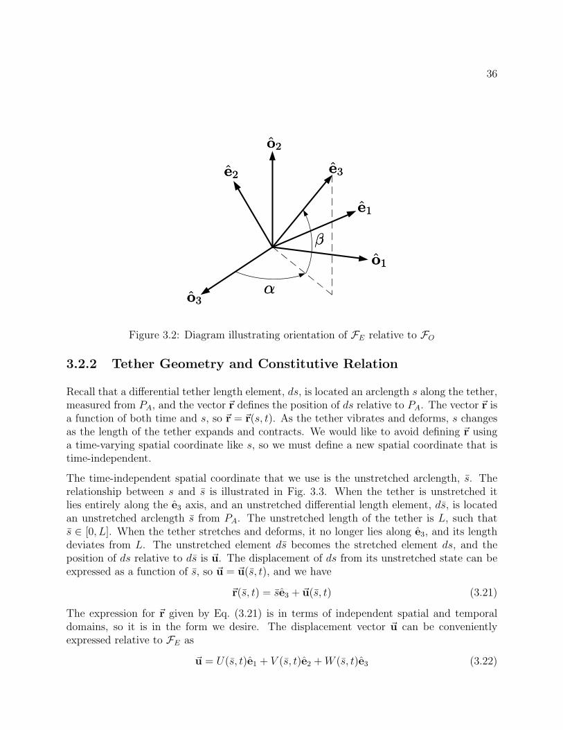
36

o1o1

o2o2

o3o3

e3e3

e1e1

e2e2

αα

ββ

Figure 3.2: Diagram illustrating orientation of FE relative to FO

3.2.2 Tether Geometry and Constitutive Relation

Recall that a differential tether length element, ds, is located an arclength s along the tether,measured from PA, and the vector ~r defines the position of ds relative to PA. The vector ~r isa function of both time and s, so ~r = ~r(s, t). As the tether vibrates and deforms, s changesas the length of the tether expands and contracts. We would like to avoid defining ~r usinga time-varying spatial coordinate like s, so we must define a new spatial coordinate that istime-independent.

The time-independent spatial coordinate that we use is the unstretched arclength, s. Therelationship between s and s is illustrated in Fig. 3.3. When the tether is unstretched itlies entirely along the e3 axis, and an unstretched differential length element, ds, is locatedan unstretched arclength s from PA. The unstretched length of the tether is L, such thats ∈ [0, L]. When the tether stretches and deforms, it no longer lies along e3, and its lengthdeviates from L. The unstretched element ds becomes the stretched element ds, and theposition of ds relative to ds is ~u. The displacement of ds from its unstretched state can beexpressed as a function of s, so ~u = ~u(s, t), and we have

~r(s, t) = se3 + ~u(s, t) (3.21)

The expression for ~r given by Eq. (3.21) is in terms of independent spatial and temporaldomains, so it is in the form we desire. The displacement vector ~u can be convenientlyexpressed relative to FE as

~u = U(s, t)e1 + V (s, t)e2 +W (s, t)e3 (3.22)

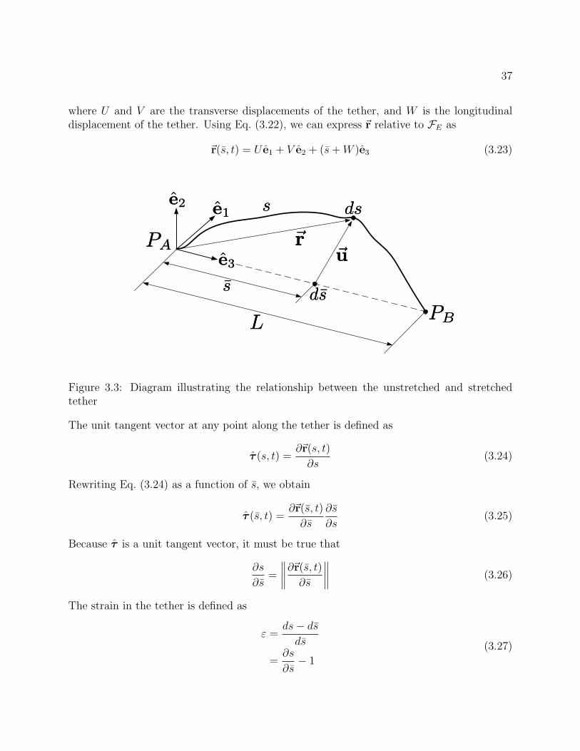
37

where U and V are the transverse displacements of the tether, and W is the longitudinaldisplacement of the tether. Using Eq. (3.22), we can express ~r relative to FE as

~r(s, t) = U e1 + V e2 + (s+W )e3 (3.23)

LL

ss

ss dsds

dsds

PBPB

PAPA rruu

e1e1e2e2

e3e3

Figure 3.3: Diagram illustrating the relationship between the unstretched and stretchedtether

The unit tangent vector at any point along the tether is defined as

τ (s, t) =∂~r(s, t)

∂s(3.24)

Rewriting Eq. (3.24) as a function of s, we obtain

τ (s, t) =∂~r(s, t)

∂s

∂s

∂s(3.25)

Because τ is a unit tangent vector, it must be true that

∂s

∂s=

∥∥∥∥∂~r(s, t)

∂s

∥∥∥∥ (3.26)

The strain in the tether is defined as

ε =ds− dsds

=∂s

∂s− 1

(3.27)

38

Using Eq. (3.26), the strain at any point in the tether is expressed as a function of s as

ε(s, t) =

∥∥∥∥∂~r(s, t)

∂s

∥∥∥∥− 1 (3.28)

Differentiating Eq. (3.28) with respect to time, the strain rate at any point along the tetheris expressed as a function of s as

ε(s, t) =1

1 + ε

[∂~r(s, t)

∂s· ∂~r(s, t)

∂s

](3.29)

The tension in the tether is modeled using the linear Kelvin-Voigt law of viscoelasticity,which expresses the axial stress in the tether, σ, in terms of the strain and strain rate as

σ = E(ε+ cε) (3.30)

where E is the Young’s modulus of the tether material and c is a structural damping constant.Because the tether is modeled as an elastic string, the tension is only due to the axial stress,and is given by

T = EA(ε+ cε) (3.31)

where A is the cross-sectional area of the tether. Note that T = T (s, t) because the strainand strain rate vary along the tether. In general, the cross sectional area may also varyalong the length of the tether. Another consequence of the assumption that the tether is anelastic string is that the tension must be in the direction of the tether unit tangent vector,so the tension vector at any point in the tether is

~T = T τ

= EA(ε+ cε)τ(3.32)

Using Eqs. (3.28) and (3.29) in Eq. (3.32) yields an expression for the tension vector in termsof the geometry of the tether.

One final point to note about the mathematical model of the tension in the tether is thatthe tension cannot be a compressive force. This fact is yet another consequence of theassumption that the tether is an elastic string. To account for this fact, we set the tensionmagnitude equal to zero at any point it is calculated to be negative using Eq. (3.31),

T =

EA(ε+ cε), ε+ cε > 00, ε+ cε < 0

(3.33)

Modeling the tension in this manner does not account for buckling of the tether at pointswhere it becomes slack, and it also does not prevent the length of the tether from becomingless than the unstretched length L when portions of the tether become slack. However,typical TSS, and spinning TSS in particular, are expected to operate in a configuration inwhich the tether remains completely tensioned, so the fact that the tension model does notcompletely account for the effects of slackness is not a concern in this work.

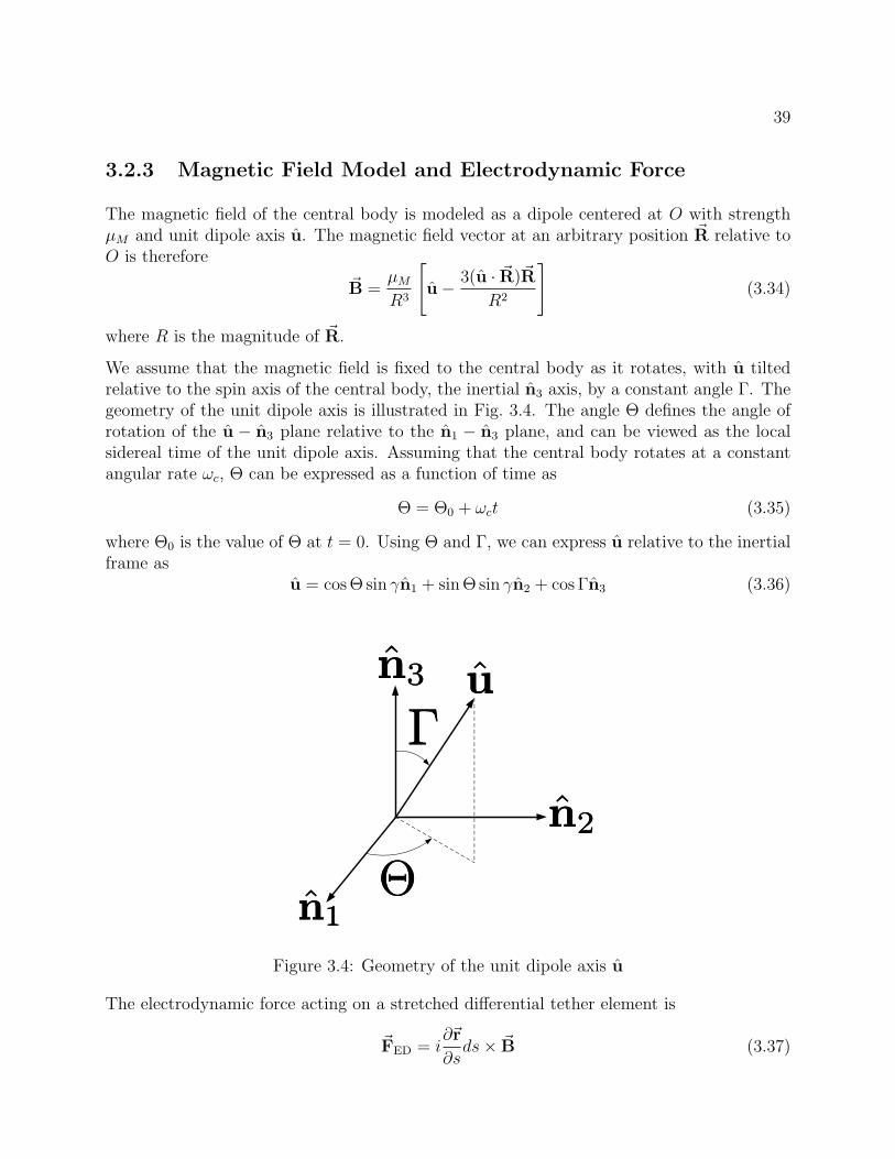
39

3.2.3 Magnetic Field Model and Electrodynamic Force

The magnetic field of the central body is modeled as a dipole centered at O with strengthµM and unit dipole axis u. The magnetic field vector at an arbitrary position ~R relative toO is therefore

~B =µMR3

[u− 3(u · ~R)~R

R2

](3.34)

where R is the magnitude of ~R.

We assume that the magnetic field is fixed to the central body as it rotates, with u tiltedrelative to the spin axis of the central body, the inertial n3 axis, by a constant angle Γ. Thegeometry of the unit dipole axis is illustrated in Fig. 3.4. The angle Θ defines the angle ofrotation of the u − n3 plane relative to the n1 − n3 plane, and can be viewed as the localsidereal time of the unit dipole axis. Assuming that the central body rotates at a constantangular rate ωc, Θ can be expressed as a function of time as

Θ = Θ0 + ωct (3.35)

where Θ0 is the value of Θ at t = 0. Using Θ and Γ, we can express u relative to the inertialframe as

u = cos Θ sin γn1 + sin Θ sin γn2 + cos Γn3 (3.36)

uu

n1n1

n2n2

n3n3

ΘΘ

ΓΓ

Figure 3.4: Geometry of the unit dipole axis u

The electrodynamic force acting on a stretched differential tether element is

~FED = i∂~r

∂sds× ~B (3.37)

40

where i is the electrical current in the tether. Noting that

∂~r

∂sds =

∂~r

∂sds (3.38)

we can also express the electrodynamic force in terms of the unstretched arclength as

~FED = i∂~r

∂sds× ~B (3.39)

In this study we are only concerned with the effects of the electrodynamic force on the systemdynamics, and not with the actual physical mechanisms responsible for the generation of theelectrodynamic force. We therefore assume that the current in the tether can be controlledto be any desired value. Recall that for an uncontrolled system the current in the tetheris dependent on the motion of the tether through the magnetic field of the central body.Because of this dependence, the current naturally varies throughout the motion of the system.We are not concerned with these naturally occurring variations because it is always possibleto include a separate power source in the system that can be used to control the current toa desired value. For this reason, we do not include a relationship such as Eq. (1.1) in themathematical model of the electrodynamic force.

3.2.4 Equations of Motion of A

The complete set of equations of motion for the primary end body, A, consists of equationsgoverning the evolution of the osculating orbit of GA, and equations governing the rotationof the body-fixed coordinate frame FA relative to FO. The latter set of equations govern theattitude motion of A relative to the orbital frame.

The orbital equations for GA are determined by applying Newton’s Second Law to A,

mA~rA = ~FGA + ~T(0, t) (3.40)

where mA is the mass of A, ~FGA is the gravitational force of the central body acting onA, and ~T(0, t) is the tether tension acting on A at the attachment point PA. Because thecentral body is treated as a point mass, the gravitational force is given by Newton’s Law ofUniversal Gravitation as

~FGA = −mAµ

r3A

~rA (3.41)

Note that Eq. (3.41) also implies that A is a point mass, despite that fact that we havemodeled A as a finite body. However, because A is small relative to its distance from O,any additional gravitational effects due to its finite dimensions are negligible relative to theNewtonian component of the gravitational force, and Eq. (3.41) is a sufficient approximation.Using Eq. (3.41) in Eq. (3.40), the orbital equation of motion for GA is written as

~rA = − µ

r3A

~rA +~T(0, t)

mA

(3.42)

41

Defining the disturbance acceleration

~aDA =~T(0, t)

mA

(3.43)

we can rewrite Eq. (3.44) in the perturbation form

~rA +µ

r3A

~rA = ~aDA (3.44)

If ~aDA = ~0, then Eq. (3.44) has the form of the equation of motion of a point mass on aKeplerian orbit. Note that Eq. (3.44) approaches this case as mA approaches infinity. Whenthe disturbance acceleration is not zero, the disturbance acceleration causes perturbationsaway from a Keplerian orbit.

The effects of the disturbance acceleration on the orbit of GA are quantified in terms ofchanges in the osculating orbit elements of GA. Express the disturbance acceleration relativeto FO as

~aDA = aDA1o1 + aDA2o2 + aDA3o3 (3.45)

where aDA1, aDA2, and aDA3 are the disturbance acceleration components in the local hori-zontal, orbit normal, and local vertical directions of the osculating orbit, respectively. UsingEq. (3.45), the evolution of the osculating orbit elements under the action of the disturbanceacceleration is governed by the Gauss form of the orbit variational equations,4,55

a =2a2

h

[(e sin ν)aDA3 +

(p

rA

)aDA1

](3.46)

e =(p sin ν)aDA3 + [(p+ rA) cos ν + rAe]aDA1

h(3.47)

I =(rA cos θ)aDA2

h(3.48)

Ω =(rA sin θ)aDA2

h sin I(3.49)

ω =−(p cos ν)aDA3 + [(p+ rA) sin ν]aDA1

he− (rA sin θ cos I)aDA2

h I(3.50)

ν =h

r2A

+(p cos ν)aDA3 − [(p+ rA) sin ν]aDA1

he(3.51)

where h =√µp is the specific angular momentum of the osculating orbit. Equations (3.46–

3.51) completely define the translational motion of GA relative to O, and thus the orbitalmotion of the system. One important point we must note about Eqs. (3.46–3.51), however,is that they contain mathematical singularities for e = 0 and sin I = 0, which correspondto circular and equatorial orbits, respectively. These singularities are due to the well-known

42

fact that ω is undefined for circular orbits and Ω is undefined for equatorial orbits. A non-singular set of osculating orbit elements, such as the equinoctial elements, could be used inplace of the classical orbit elements, but the classical elements are sufficient for our purposesbecause an actual TSS is unlikely to ever be on exactly a circular or equatorial orbit.

Th rotational equations of motion of A are determined by applying Euler’s rotational equa-tions to A,

~IA · ~ωA/N + ~ωA/N ×~IA · ~ωA/N = ~MGA + ~pA × ~T(0, t) (3.52)

where ~IA is the centroidal moment of inertia tensor of A, ~ωA/N is the angular velocity of FArelative to FN ,

~ωA/N = ~ωA/O + ~ωO/N (3.53)

and ~MGA is the gravity-gradient torque acting on A about GA. Because the size of A is smallrelative to its orbit radius, we use a linear approximation for the gravity-gradient torque,23,55

~MGA =3µ

r5A

~rA ×~IA ·~rA (3.54)

Using Eq. (3.54) in Eq. (3.52), the rotational equations of motion of A are written as

~IA · ~ωA/N + ~ωA/N ×~IA · ~ωA/N =3µ

r5A

~rA ×~IA ·~rA + ~pA × ~T(0, t) (3.55)

When expressed relative to FA and combined with the kinematic relationship defined byEq. (3.17), the rotational equations of motion govern the evolution of the quaternion qA,and thus the orientation of FA relative to FO. Because FA is a body-fixed coordinate framefor the rigid body FA, the orientation of FA relative to FO defines the attitude of A relativeto the orbital frame.

3.2.5 Equations of Motion of the Tether

The motion of the tether can be decomposed into two separate modes. The first mode isrepresented by the motion of the coordinate axis e3 relative to FO. Recall that e3 points fromPA to PB, and the undeformed tether lies entirely along e3. The motion of e3 relative to FOtherefore defines the pendular mode of the tether motion relative to the orbital frame. Thesecond mode of the tether motion is the elastic vibrations of the tether. These vibrationsdefine the deformation of the tether away from its undeformed alignment with e3. Each ofthese two separate modes of motion have a different set of governing equations of motion.The equations of motion for the pendular mode govern the evolution of the tether attitudeangles α and β, and the equations of motion for the elastic vibration mode govern theevolution of the tether displacements U , V , and W .

The equations of motion for the pendular mode of the tether motion are derived by firstapplying Newton’s Second Law to B,

mB~rB = ~FGB − ~T(L, t) (3.56)

43

where ~rB is the position of GB relative to O, mB is the mass of B, ~FGB is the gravitationalforce of the central body acting on B, and ~T(L, t) is the tether tension acting on B at theattachment point PB. As done with A, the gravitational force acting on B is modeled usingNewton’s Law of Universal Gravitation,

~FGB = −mBµ

r3B

~rB (3.57)

where rB is the magnitude of ~rB. Using Eq. (3.57) in Eq. (3.56), the translational equationof motion of B is written as

~rB =~FB

mB

(3.58)

where ~FB is the total external force vector acting on B,

~FB = −mBµ

r3B

~rB − ~T(L, t) (3.59)

Noting that ~rB can be written as

~rB = ~rA + ~pA +~r(L, t)− ~pB (3.60)

Eq.(3.58) is written as

~r(L, t) = ~aL (3.61)

where we have defined the acceleration quantity

~aL =~FB

mB

− ~rA − ~pA + ~pB (3.62)

Noting that there cannot be any transverse displacement of the tether at either of its ends,we can express ~r(L, t) as

~r(L, t) = [L+W (L, t)]e3 (3.63)

and the inertial derivative on the left-hand-side of Eq. (3.61) is written as

~r(L, t) = rL1e1 + rL2e2 + rL3e3 (3.64)

where

rL1 = 2W (L, t)(α + θ) cos β + [L+W (L, t)][(α + θ) cos β − 2(α + θ)β sin β] (3.65)

rL2 = 2W (L, t)β + [L+W (L, t)][β + (α + θ)2 sin β cos β] (3.66)

rL3 = W (L, t)− [L+W (L, t)][(α + θ)2 cos2 β + β2] (3.67)

Note that the quantities θ and θ are defined in Eqs. (3.3) and (3.4). Expressing ~aL relativeto FE as

~aL = aL1e1 + aL2e2 + aL3e3 (3.68)

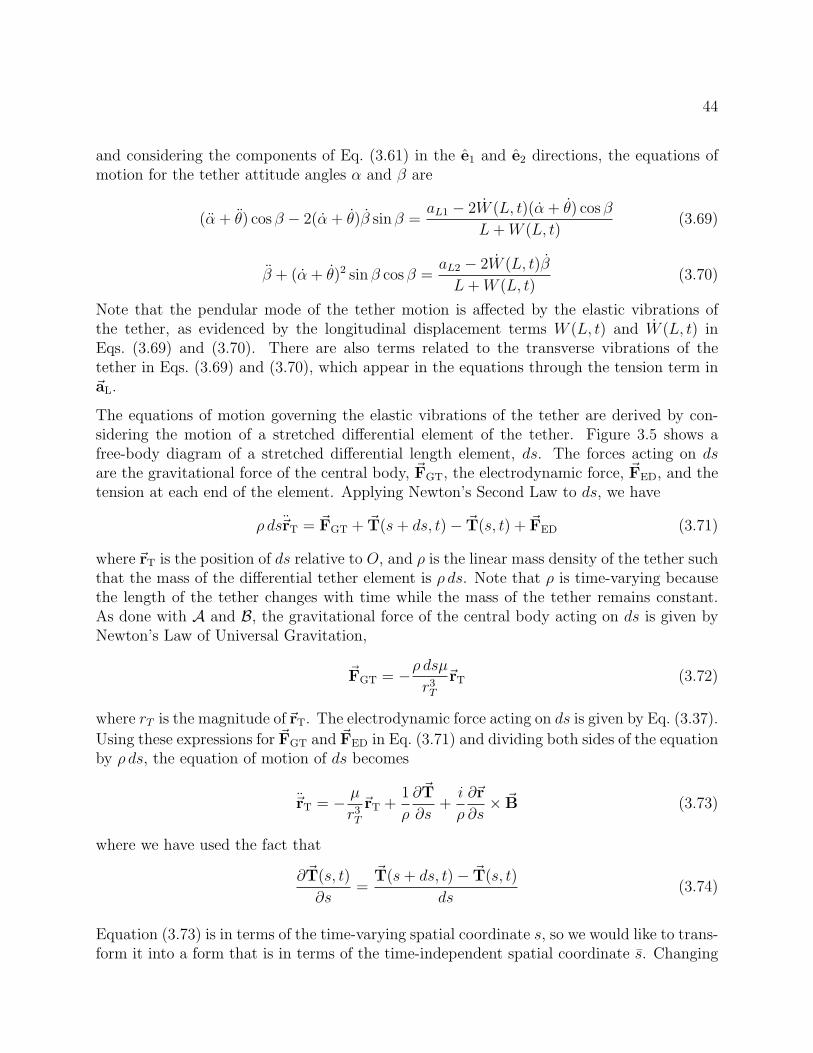
44

and considering the components of Eq. (3.61) in the e1 and e2 directions, the equations ofmotion for the tether attitude angles α and β are

(α + θ) cos β − 2(α + θ)β sin β =aL1 − 2W (L, t)(α + θ) cos β

L+W (L, t)(3.69)

β + (α + θ)2 sin β cos β =aL2 − 2W (L, t)β

L+W (L, t)(3.70)

Note that the pendular mode of the tether motion is affected by the elastic vibrations ofthe tether, as evidenced by the longitudinal displacement terms W (L, t) and W (L, t) inEqs. (3.69) and (3.70). There are also terms related to the transverse vibrations of thetether in Eqs. (3.69) and (3.70), which appear in the equations through the tension term in~aL.

The equations of motion governing the elastic vibrations of the tether are derived by con-sidering the motion of a stretched differential element of the tether. Figure 3.5 shows afree-body diagram of a stretched differential length element, ds. The forces acting on dsare the gravitational force of the central body, ~FGT, the electrodynamic force, ~FED, and thetension at each end of the element. Applying Newton’s Second Law to ds, we have

ρ ds~rT = ~FGT + ~T(s+ ds, t)− ~T(s, t) + ~FED (3.71)

where ~rT is the position of ds relative to O, and ρ is the linear mass density of the tether suchthat the mass of the differential tether element is ρ ds. Note that ρ is time-varying becausethe length of the tether changes with time while the mass of the tether remains constant.As done with A and B, the gravitational force of the central body acting on ds is given byNewton’s Law of Universal Gravitation,

~FGT = −ρ dsµr3T

~rT (3.72)

where rT is the magnitude of~rT. The electrodynamic force acting on ds is given by Eq. (3.37).

Using these expressions for ~FGT and ~FED in Eq. (3.71) and dividing both sides of the equationby ρ ds, the equation of motion of ds becomes

~rT = − µ

r3T

~rT +1

ρ

∂~T

∂s+i

ρ

∂~r

∂s× ~B (3.73)

where we have used the fact that

∂~T(s, t)

∂s=~T(s+ ds, t)− ~T(s, t)

ds(3.74)

Equation (3.73) is in terms of the time-varying spatial coordinate s, so we would like to trans-form it into a form that is in terms of the time-independent spatial coordinate s. Changing

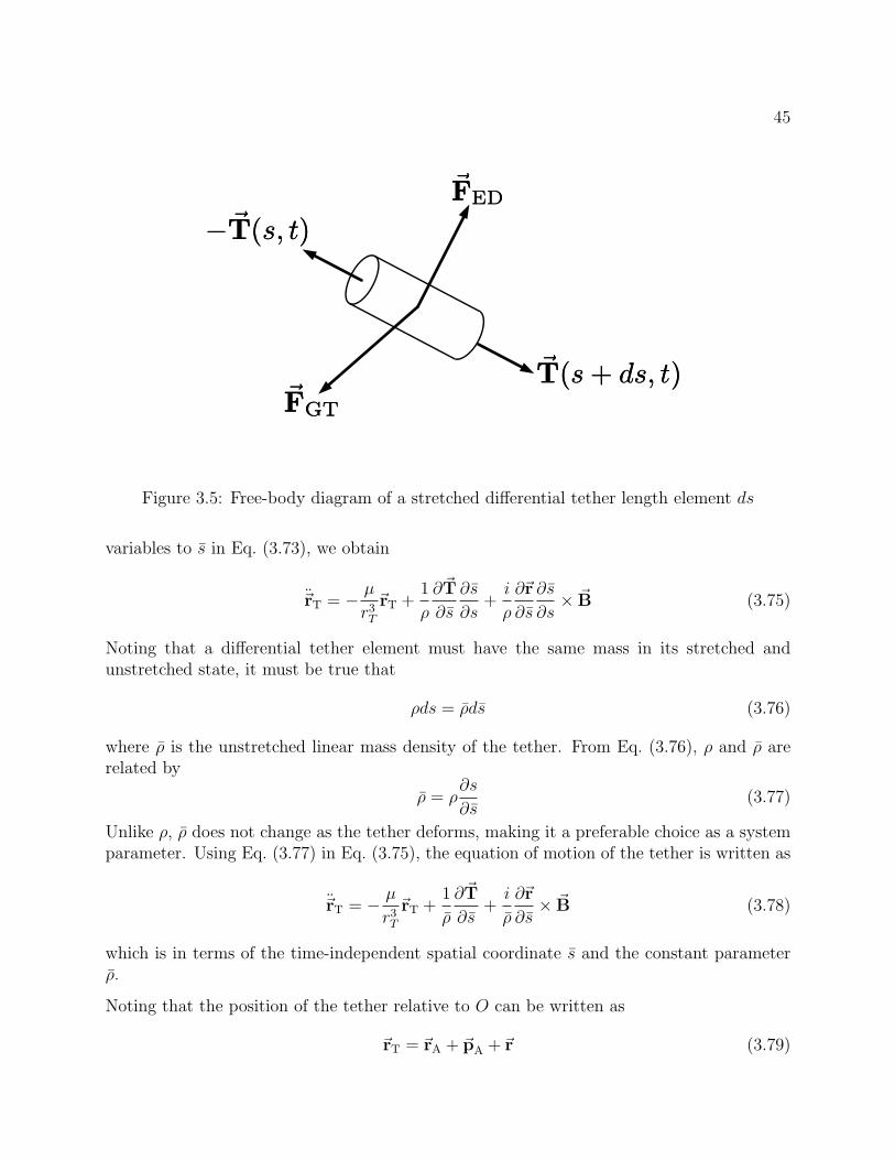
45

FGTFGT

FEDFED

T(s+ ds, t)T(s+ ds, t)

−T(s, t)−T(s, t)

Figure 3.5: Free-body diagram of a stretched differential tether length element ds

variables to s in Eq. (3.73), we obtain

~rT = − µ

r3T

~rT +1

ρ

∂~T

∂s

∂s

∂s+i

ρ

∂~r

∂s

∂s

∂s× ~B (3.75)

Noting that a differential tether element must have the same mass in its stretched andunstretched state, it must be true that

ρds = ρds (3.76)

where ρ is the unstretched linear mass density of the tether. From Eq. (3.76), ρ and ρ arerelated by

ρ = ρ∂s

∂s(3.77)

Unlike ρ, ρ does not change as the tether deforms, making it a preferable choice as a systemparameter. Using Eq. (3.77) in Eq. (3.75), the equation of motion of the tether is written as

~rT = − µ

r3T

~rT +1

ρ

∂~T

∂s+i

ρ

∂~r

∂s× ~B (3.78)

which is in terms of the time-independent spatial coordinate s and the constant parameterρ.

Noting that the position of the tether relative to O can be written as

~rT = ~rA + ~pA +~r (3.79)

46

the tether equation of motion can be further rewritten as

~r = − µ

r3T

~rT +1

ρ

∂~T

∂s+i

ρ

∂~r

∂s× ~B− ~rA − ~pA (3.80)

Equation (3.80) is a partial differential equation that governs the evolution of the shape ofthe tether relative to PA. The boundary condition of Eq. (3.80) at PA is

~r(0, t) = ~0 (3.81)

and the boundary condition of Eq. (3.80) at PB is given by Eq. (3.61).

Using the expression for ~r(s, t) given by Eq. (3.23) and expressing Eq. (3.80) relative toFE yields partial differential equations for the tether vibration coordinates U , V , and W .Because there can be no transverse displacement at the ends of the tether, the boundaryconditions for U and V are

U(0, t) = U(L, t) = 0 (3.82)

V (0, t) = V (L, t) = 0 (3.83)

From Eq. (3.81), the boundary condition of the longitudinal displacement at PA is

W (0, t) = 0 (3.84)

The boundary condition of the longitudinal displacement at PB is determined by taking thecomponent of Eq. (3.61) in the e3 direction,

W (L, t) = aL3 + [L+W (L, t)][(α + θ)2 cos2 β + β2] (3.85)

The complete set of equations of motion of the tether is given by Eqs. (3.69), (3.70), and(3.80), combined with the boundary conditions defined in Eqs. (3.81) and (3.61). The pen-dular motion of the tether is governed by Eqs. (3.69) and (3.70), and the elastic vibrationsare governed by Eq. (3.80). Note that the pendular and vibration modes of the tether motionare not independent, in that the elastic vibrations affect the pendular motion and visa versa.

3.2.6 Equations of Motion of B

Given the orbital motion of GA, the attitude motion of A, and the motion of the tether,we can determine the motion of the tether attachment point PB on B. The motion of PBdefines the translational motion of B, so we do not need to derive equations of motion forthe translational motion of B. The only equations of motion we must determine are thosethat govern the attitude motion of B relative to FO.

47

As done with A, the attitude equations of motion of B are derived using Euler’s rotationalequations,

~IB · ~ωB/N + ~ωB/N ×~IB · ~ωB/N = ~MGB − ~pB × ~T(L, t) (3.86)

where ~IB is the centroidal moment of inertia tensor of B, ~ωB/N is the angular velocity of FBrelative to FN ,

~ωB/N = ~ωB/O + ~ωO/N (3.87)

and ~MGB is the gravity-gradient torque acting on B about GB. We once again use a linearapproximation for the gravity-gradient torque,

~MGB =3µ

r5B

~rB ×~IB ·~rB (3.88)

Using Eq. (3.88) in Eq. (3.86), the rotational equations of motion of B are

~IB · ~ωB/N + ~ωB/N ×~IB · ~ωB/N =3µ

r5B

~rB ×~IB ·~rB − ~pB × ~T(L, t) (3.89)

When expressed relative to FB and combined with the kinematic relationship defined byEq. (3.17), the rotational equations of motion of B govern the evolution of the quaternionqB, and thus the attitude motion of B relative to FO.

3.2.7 Summary of the Mathematical Model

The mathematical model presented in this section defines the equations of motion governingthe various aspects of the system dynamics. These aspects are the orbital motion of thesystem, the attitude motion of the end bodies, and the motion of the tether. Equations (3.46–3.51) govern the evolution of the osculating orbit elements of GA, and thus the orbital motionof the system. The equations of motion for the attitude of A are given by Eq. (3.55).The pendular motion of the tether is governed by Eqs. (3.69) and (3.70), and the elasticvibrations of the tether are governed by Eq. (3.80). The boundary conditions for the tetherelastic vibrations are defined by Eqs. (3.81) and (3.61). Equation (3.89) governs the attitudemotion of B.

The complete set of equations of motion that comprise the mathematical model is a mix ofordinary and partial differential equations. These equations are coupled and highly nonlinear,making a direct analytical treatment of them completely intractable. This is not unexpected,however, because the top-level model is intended to be the model that is the most complicatedpossible, yet still practical from a computational standpoint. Any computational modelfor the mathematical model must therefore consist entirely of numerical solutions of themathematical model. In the next section, we present two such computational models.

48

3.3 Computational Models

The computational models for the mathematical model presented in the previous sectionconsist entirely of the tools required to produce numerical solutions to the system equations ofmotion. To determine these numerical solutions, the equations of motion must be discretizedand a computer program must be written to numerically solve the discretized equations ofmotion. Because the equations of motion governing the elastic vibrations of the tether arepartial differential equations, they must be discretized in both time and space. The equationsof motion governing the system orbital motion, end body attitude motion, and the pendularmotion of the tether are ordinary differential equations that must only be discretized in time.

In this section, we present two different computational models based on two different methodsof spatially discretizing the equations of motion for the tether elastic vibrations. The firstmethod is the assumed modes method (AMM), and the second method is the finite elementmethod (FEM). In both of these methods, the partial differential equations governing thetether elastic vibrations are transformed into a finite set of ordinary differential equations.This set of ordinary differential equations is then temporally discretized, and the full set ofdiscretized equations of motion can be used to determine numerical solutions for the systemmotion.

3.3.1 Assumed Modes Method

The assumed modes method is one of the more common methods of spatially discretizing thepartial differential equations governing the elastic vibrations of the tether. Several studiesthat have applied the AMM to non-electrodynamic TSS are those by Beletsky and Levin,5

Ruiz et al.,53 and Pradhan et al.50 The discretization procedure presented below is similarto those used in these studies, with the exception that the electrodynamic force acting alongthe tether is taken into account.

To spatially discretize the tether vibration equations of motion using the AMM, we beginwith Eq. (3.80) and rewrite the inertial derivative on the left-hand side of the equation as

~r =~r + ~ωE/N ×~r + ~ωE/N × (~ωE/N ×~r) + 2~ωE/N ×

~r (3.90)

where

( ) denotes a time-derivative as seen by FE. Using Eq. (3.90) in Eq. (3.80) and definingthe acceleration quantity

~aT =− µ

r3T

~rT +1

ρ

∂~T

∂s+i

ρ

∂~r

∂s× ~B− ~rA − ~pA

− ~ωE/N ×~r− ~ωE/N × (~ωE/N ×~r)− 2~ωE/N ×~r

(3.91)

the equation of motion for the tether elastic vibrations is written as~r = ~aT (3.92)

49

From Eq. (3.23), the left-hand side of Eq. (3.92) is~r = U e1 + V e2 + W e3 (3.93)

Expressing ~aT relative to FE as

~aT = aT1e1 + aT2e2 + aT3e3 (3.94)

and using Eq. (3.93) and (3.94) in Eq.(3.92), the vibration equations of motion are writtenin terms of the tether displacements as

U = aT1 (3.95)

V = aT2 (3.96)

W = aT3 (3.97)

The boundary conditions of Eq. (3.95–3.97) are given by Eqs. (3.82–3.85).

Next, we assume that each tether displacement can be expressed as a finite sum of productsof time-dependent generalized coordinates, Cij(t), and spatially-dependent assumed modefunctions, Nij(s),

U(s, t) =

NT∑j=1

C1j(t)N1j(s) (3.98)

V (s, t) =

NT∑j=1

C2j(t)N2j(s) (3.99)

W (s, t) =

NL∑j=1

C3j(t)N1j(s) (3.100)

where NT is the number of transverse assumed modes and NL is the number of longitudinalassumed modes. Note that the numbers of transverse and longitudinal assumed modes canbe different. The only constraints on the assumed mode functions are that they form alinearly independent, complete set, and that they satisfy the geometric boundary conditionsof the tether. Recall that the geometric boundary conditions of the tether are given byEqs. (3.82–3.84). Substituting the assumed solution forms defined by Eqs. (3.98–3.100) intoEqs. (3.95–3.97), we obtain

NT∑j=1

C1jN1j = aT1 (3.101)

NT∑j=1

C2jN2j = aT2 (3.102)

NL∑j=1

C3jN3j = aT3 (3.103)

50

The final step in the AMM discretization is to apply the Galerkin method38 to Eqs. (3.101–3.103); however, we must consider the transverse and longitudinal vibrations separatelybecause of the form of their respective boundary conditions.

For i = 1, . . . , NT , multiply Eq. (3.101) by N1i and multiply Eq. (3.102) by N2i, then integrateover the length of the tether to obtain

NT∑j=1

m1ijC1j = aT1i , i = 1, . . . , NT (3.104)

NT∑j=1

m2ijC2j = aT2i , i = 1, . . . , NT (3.105)

where we have defined

mkij =

∫ L

0

NkiNkj ds (3.106)

aTki =

∫ L

0

aTkNki ds (3.107)

Equations (3.104) and (3.105) each define a set of NT ordinary differential equations for theNT generalized coordinates Cij. Defining the matrices

Mk = [mkij] (3.108)

aTk = [aTki] (3.109)

Ck = [Cki] (3.110)

we can express each of Eqs. (3.104) and (3.105) in matrix form as

MkCk = aTk (3.111)

Equation (3.111) defines the spatially discretized equations of motion for the transverse vi-brations of the tether. In this work, the assumed mode functions for the transverse vibrationsare taken as

Nij =√

2 sin

(jπ

Ls

)(3.112)

Note that these assumed mode functions satisfy the geometric boundary conditions for thetransverse vibrations defined in Eqs. (3.82) and (3.83). These functions are also orthonormal,such that the mass matrices simplify to

Mk = 1 (3.113)

where 1 is the identity matrix.

51

Considering now the equations for the longitudinal vibrations, multiplying Eq. (3.103) byN3i for i = 1, . . . , NL − 1 and integrating over the length of the tether, we obtain

NL∑j=1

m3ijC3j = aT3i , i = 1, . . . , NL − 1 (3.114)

where m3ij and aT3i are defined as in Eqs. (3.106) and (3.107). We do not multiply by theassumed mode function and integrate over the tether for i = 1, . . . , NL in this case becausewe want to include an equation that accounts for the dynamic boundary condition of thelongitudinal vibrations, which is defined by Eq. (3.85). Using Eq. (3.100) in Eq. (3.85), wehave

NL∑j=1

C3jN3j(L) = aL3 +

[L+

NL∑j=1

C3jN3j(L)

][(α + θ)2 cos2 β + β2] (3.115)

Equations (3.114) and (3.115) define a set of NL ordinary differential equations for the NL

generalized coordinates C3j. Defining the matrices

M3 =

m311 . . . m31NL...

. . ....

N31(L) . . . N3NL(L)

(3.116)

aT3 =

aT31

...

aL3 +[L+

∑NLj=1 C3jN3j(L)

][(α + θ)2 cos2 β + β2]

(3.117)

and using Eq. (3.110), we can express Eqs. (3.114) and (3.115) in matrix form as

M3C3 = aT3 (3.118)

Equation (3.118) defines the spatially discretized equations of motion for the longitudinalvibrations of the tether. The shape functions for the longitudinal vibration are taken as

N3j(s) =( sL

)j(3.119)

Note that these assumed mode functions satisfy the geometric boundary condition givenby Eq. (3.84). Unlike the transverse assumed mode functions, however, the longitudinalassumed mode functions are not orthogonal. This means that the mass matrix M3 is fullypopulated, and taking its inverse in Eq. (3.118) will become increasingly computationallyintensive as NL increases.

The complete set of spatially discretized equations of motion for the tether elastic vibrationsis given by Eqs. (3.111) and (3.118). Combining these equations with the equations of motion

52

for the system orbital motion, end body attitude motion, and pendular tether motion formsa set of ordinary differential equations for the entire motion of the system. This set ofordinary differential equations is temporally discretized and solved numerically using thebuilt-in MATLAB function ode15s, which uses a variable-order method based on numericaldifferentiation formulas to solve stiff systems of ordinary differential equations and differentialalgebraic equations. Note that these numerical solutions are approximate solutions for thesystem equations of motion, and they should approach the solution of the equations of motionas both the temporal and spatial discretizations are refined.

3.3.2 Finite Element Method

The finite element method is a far less commonly used spatial discretization method for TSSdynamics than is the AMM. One application of the FEM to a TSS is that of Steiner etal.,61 in which the dynamics of a system consisting of two rigid end bodies connected by aflexible, variable length tether are numerically simulated. Another study that applied theFEM to a similar problem is that by Kuhn et al.;29 however, the system considered in thisstudy is a simple string pendulum, and not a TSS. In what is presented below, we use asimilar procedure to that used in these works to apply the FEM to a TSS that includeselectrodynamic forcing.

In the FEM discretization, we begin by writing Eq. (3.80) in the weak form. Let Ni(s) bea shape function defined over the length of the tether. Multiplying Eq. (3.80) by Ni andintegrating over the tether, we obtain∫ L

0

~rNids =

∫ L

0

(− µ

r3T

~rT +1

ρ

∂~T

∂s+i

ρ

∂~r

∂s× ~B− ~rA − ~pA

)Nids (3.120)

Integrating the tension term in Eq. (3.120) by parts, we have∫ L

0

1

ρ

∂~T

∂sds =

1

ρ

[~T(L, t)Ni(L)− ~T(0, t)Ni(0)−

∫ L

0

~TdNi

dsds

](3.121)

From Eqs. (3.40) and (3.58), the tension at the ends of the tether can be written as

~T(0, t) = mA

(~rA +

µ

r3A

~rA

)(3.122)

~T(L, t) = −mB

(~rB +

µ

r3B

~rB

)(3.123)

Using Eqs. (3.122) and (3.123) in Eq. (3.121), and using the resulting expression in Eq. (3.120),we obtain∫ L

0

~rNids =

∫ L

0

(− µ

r3T

~rT +i

ρ

∂~r

∂s× ~B− ~rA − ~pA

)Nids−

∫ L

0

1

ρ~TdNi

dsds

− mA

ρ

(~rA +

µ

r3A

~rA

)Ni(0)− mB

ρ

(~rB +

µ

r3B

~rB

)Ni(L)

(3.124)

53

Recalling that ~rT = ~rA +~pA +~r and ~rB = ~rA +~pA +~r(L, t)−~pB, and defining the quantities

γ1i =

∫ L

0

Nids+mB

ρNi(L) +

mA

ρNi(0) (3.125)

γ2i =

∫ L

0

Nids+mB

ρNi(L) (3.126)

γ3i =mB

ρNi(L) (3.127)

~gi = −µ[∫ L

0

~rT

r3T

Nids+mB

ρ

~rB

r3B

Ni(L) +mA

ρ

~rA

r3A

Ni(0)

](3.128)

~fi = −1

ρ

∫ L

0

~TdNi

dsds+

i

ρ

∫ L

0

∂~r

∂s× ~BNids (3.129)

Eq. (3.124) is rewritten as∫ L

0

~rNids+mB

ρ~r(L, t)Ni(L) = −γ1i~rA − γ2i~pA + γ3i~pB + ~gi +~fi (3.130)

Equation (3.130) is the desired weak form of the equation of motion of the tether elasticvibrations.

As done in the AMM discretization, in the FEM discretization we assume that the tetherdisplacements can be written as finite sums of products of time-dependent generalized coor-dinates, Cij(t), and spatially-dependent shape functions, Nj(s),

U(s, t) =n∑j=1

C1j(t)Nj(s) (3.131)

V (s, t) =n∑j=1

C2j(t)Nj(s) (3.132)

W (s, t) =n∑j=1

C3j(t)Nj(s) (3.133)

where n is the number of assumed degrees of freedom for the tether displacements. At thispoint we must note that there are two fundamental differences between the AMM and FEMdiscretizations. First, in the FEM the assumed solution form for all three displacements usethe same shape function, whereas in the AMM different functions are used for the transverseand longitudinal displacements. The second difference between the discretization methodsis related to the generalized coordinates used in the assumed solution forms for the tetherdisplacements. In the AMM, the generalized coordinates are simply coefficients in seriesrepresentations of the tether displacements. In the FEM, however, physical significance is

54

attached to the generalized coordinates by taking them as values of displacements, slopes, orcurvatures at various points along the tether. These points are called nodes, and the length oftether between two nodes is called a finite element. Because the generalized coordinates rep-resent actual physical quantities, the shape functions in the FEM are interpolation functionsfor those physical quantities. This last point underscores the second fundamental differencebetween the AMM and FEM discretizations: the assumed solution in the AMM takes theform of a series representation, whereas the assumed solution in the FEM takes the form ofan interpolation function.

Using the assumed solution forms defined by Eqs. (3.131–3.132) along with Eq. (3.90), theequations of motion for the tether elastic vibrations become

n∑j=1

mij

[C1j − 2(C2j sin β − C3j cos β)(α + θ)− C1j(α + θ)2 − (C2j sin β − C3j cos β)(α + θ)

−2(C2j cos β + C3j sin β)(α + θ)β sin β]

= −γ1irA1 − γ2ipA1 + γ3ipB1 − γ4i

[(α + θ) sin β + 2(α + θ)β cos β

]+ gi1 + fi1

(3.134)

n∑j=1

mij

[C2j + 2C1j(α + θ) sin β + 2C3jβ + C1j(α + θ) sin β + C1j(α + θ)β cos β

−(C2j sin β − C3j cos β)(α + θ)2 sin β − C2jβ2 + C3jβ

]= −γ1irA2 − γ2ipA2 + γ3ipB2 − γ4i

[β + (α + θ)2 sin β cos β

]+ gi2 + fi2

(3.135)

n∑j=1

mij

[C3j − 2C1j(α + θ)β cos β − 2C2jβ − C1j(α + θ) cos β − C2jβ

−C2j(α + θ)2 sin β cos β − C3j(α + θ)2 cos2 β − C3jβ2]

= −γ1irA3 − γ2ipA3 + γ3ipB3 − γ4i

[(α + θ)2 cos2 β + β2

]+ gi3 + fi3

(3.136)

where we have defined the quantities

mij =

∫ L

0

NiNjds (3.137)

γ4i =

∫ L

0

sNids (3.138)

In Eqs. (3.134–3.136), the quantities rAj, pAj, pBj, gij, and fij represent the components of

the vectors ~rA, ~pA, ~pB, ~gi, and ~fi in the ej direction.

Equations (3.134–3.136) apply for i = 1, . . . , n, so they form a set of 3n ordinary differentialequations for the 3n nodal coordinates, Cij. Note, however, that several of the Cij are fixed

55

because they must satisfy the boundary conditions of the tether. At this point, Eqs. (3.134–3.136) are in a general form that applies to any choice of finite element and global shapefunctions. We now specialize these equations so that they apply to the particular system weare considering.

Let the tether be partitioned into Ne uniform finite elements, each with a length of

`e =L

Ne

(3.139)

Each element contains two nodes, with each node located at one of the ends of the element.We want the solution for each displacement to have continuity of displacement and slope sothat there are no physically unrealistic kinks in the shape of the tether. We therefore usethe displacement and displacement derivative (slope) at each node as the nodal degrees offreedom. Each element therefore contains four degrees of freedom: a displacement and slopeat each end of the element.

Define the element natural coordinate ξ as

ξ =s− s0

sf − s0

=s− s0

`e

(3.140)

where s0 and sf are the values of s at the beginning and end of a particular element,respectively. Note that the element natural coordinate is defined in the range ξ ∈ [0, 1].Because each element contains four degrees of freedom, we can interpolate each displacement(we consider U from here on, put what is presented applies to V and W as well) using athird-order polynomial as

U e(ξ, t) = c0 + c1ξ + c2ξ2 + c3ξ

3 (3.141)

where ci are constant coefficients. Note that U e is the displacement for a particular element,and not the displacement for the entire tether. The global displacement profile is determinedby piecing together all of the element displacement profiles, such as the one in Eq. (3.141).The degrees of freedom of the element serve as boundary conditions for Eq. (3.141), so theelement displacement profile must satisfy

U e(0, t) = c0 (3.142)

dU e(0, t)

dξ= c1 (3.143)

U e(1, t) = c0 + c1 + c2 + c3 (3.144)

dU e(1, t)

dξ= c1 + 2c2 + 3c3 (3.145)

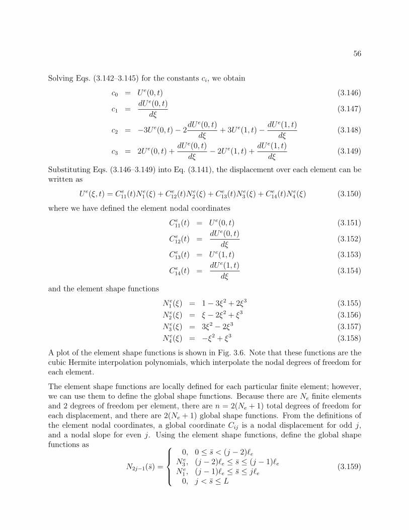
56

Solving Eqs. (3.142–3.145) for the constants ci, we obtain

c0 = U e(0, t) (3.146)

c1 =dU e(0, t)

dξ(3.147)

c2 = −3U e(0, t)− 2dU e(0, t)

dξ+ 3U e(1, t)− dU e(1, t)

dξ(3.148)

c3 = 2U e(0, t) +dU e(0, t)

dξ− 2U e(1, t) +

dU e(1, t)

dξ(3.149)

Substituting Eqs. (3.146–3.149) into Eq. (3.141), the displacement over each element can bewritten as

U e(ξ, t) = Ce11(t)N e

1 (ξ) + Ce12(t)N e

2 (ξ) + Ce13(t)N e

3 (ξ) + Ce14(t)N e

4 (ξ) (3.150)

where we have defined the element nodal coordinates

Ce11(t) = U e(0, t) (3.151)

Ce12(t) =

dU e(0, t)

dξ(3.152)

Ce13(t) = U e(1, t) (3.153)

Ce14(t) =

dU e(1, t)

dξ(3.154)

and the element shape functions

N e1 (ξ) = 1− 3ξ2 + 2ξ3 (3.155)

N e2 (ξ) = ξ − 2ξ2 + ξ3 (3.156)

N e3 (ξ) = 3ξ2 − 2ξ3 (3.157)

N e4 (ξ) = −ξ2 + ξ3 (3.158)

A plot of the element shape functions is shown in Fig. 3.6. Note that these functions are thecubic Hermite interpolation polynomials, which interpolate the nodal degrees of freedom foreach element.

The element shape functions are locally defined for each particular finite element; however,we can use them to define the global shape functions. Because there are Ne finite elementsand 2 degrees of freedom per element, there are n = 2(Ne + 1) total degrees of freedom foreach displacement, and there are 2(Ne + 1) global shape functions. From the definitions ofthe element nodal coordinates, a global coordinate Cij is a nodal displacement for odd j,and a nodal slope for even j. Using the element shape functions, define the global shapefunctions as

N2j−1(s) =

0, 0 ≤ s < (j − 2)è

N e3 , (j − 2)è ≤ s ≤ (j − 1)è

N e1 , (j − 1)è ≤ s ≤ jè0, j < s ≤ L

(3.159)

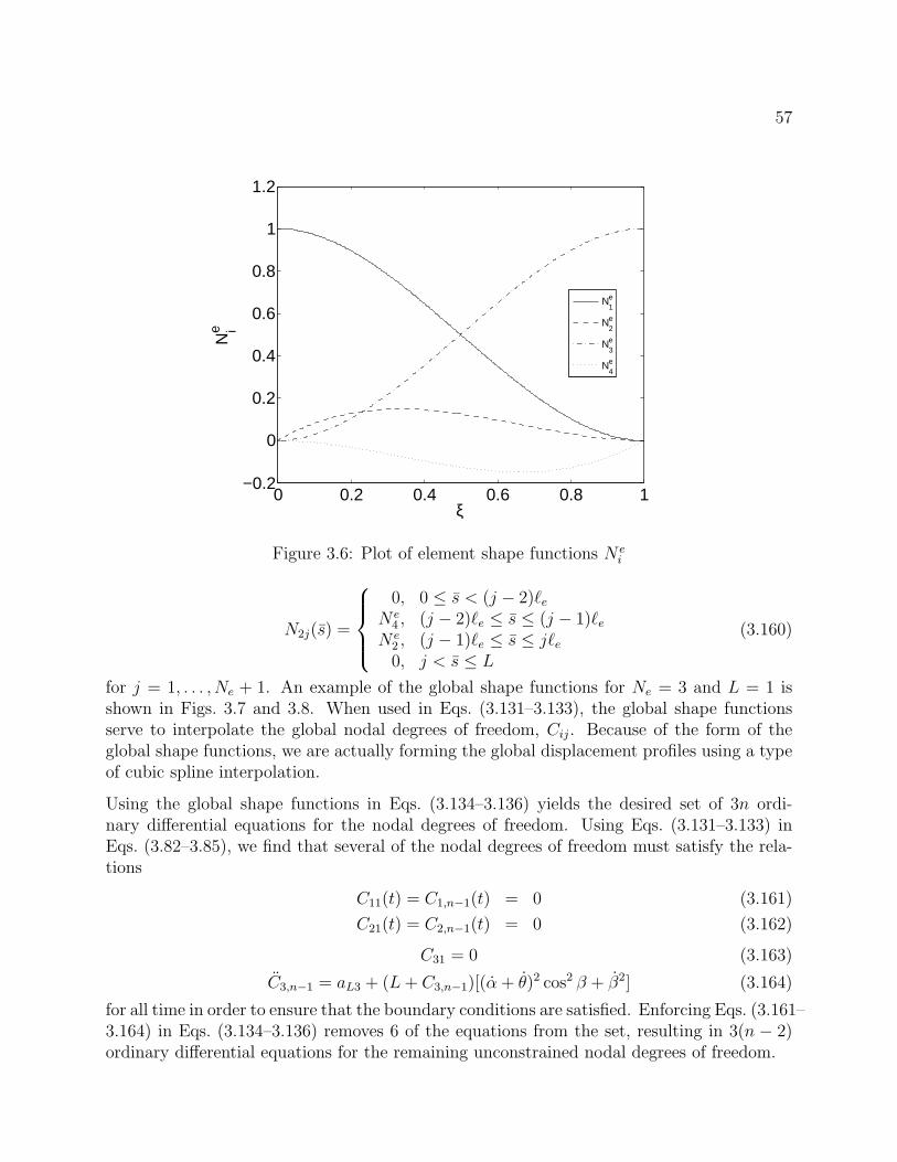
57

0 0.2 0.4 0.6 0.8 1−0.2

0

0.2

0.4

0.6

0.8

1

1.2

ξ

Nie

N1e

N2e

N3e

N4e

Figure 3.6: Plot of element shape functions N ei

N2j(s) =

0, 0 ≤ s < (j − 2)è

N e4 , (j − 2)è ≤ s ≤ (j − 1)è

N e2 , (j − 1)è ≤ s ≤ jè0, j < s ≤ L

(3.160)

for j = 1, . . . , Ne + 1. An example of the global shape functions for Ne = 3 and L = 1 isshown in Figs. 3.7 and 3.8. When used in Eqs. (3.131–3.133), the global shape functionsserve to interpolate the global nodal degrees of freedom, Cij. Because of the form of theglobal shape functions, we are actually forming the global displacement profiles using a typeof cubic spline interpolation.

Using the global shape functions in Eqs. (3.134–3.136) yields the desired set of 3n ordi-nary differential equations for the nodal degrees of freedom. Using Eqs. (3.131–3.133) inEqs. (3.82–3.85), we find that several of the nodal degrees of freedom must satisfy the rela-tions

C11(t) = C1,n−1(t) = 0 (3.161)

C21(t) = C2,n−1(t) = 0 (3.162)

C31 = 0 (3.163)

C3,n−1 = aL3 + (L+ C3,n−1)[(α + θ)2 cos2 β + β2] (3.164)

for all time in order to ensure that the boundary conditions are satisfied. Enforcing Eqs. (3.161–3.164) in Eqs. (3.134–3.136) removes 6 of the equations from the set, resulting in 3(n − 2)ordinary differential equations for the remaining unconstrained nodal degrees of freedom.

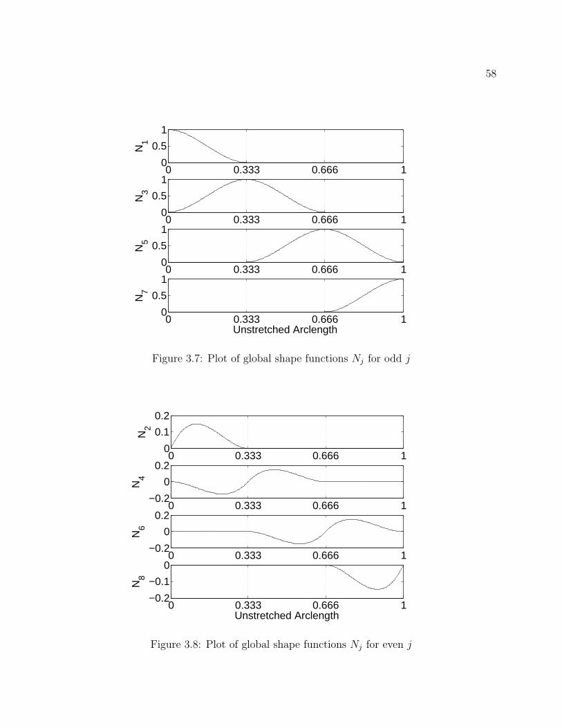
58

0 0.333 0.666 10

0.5

1N

1

0 0.333 0.666 10

0.5

1

N3

0 0.333 0.666 10

0.5

1

N5

0 0.333 0.666 10

0.5

1

N7

Unstretched Arclength

Figure 3.7: Plot of global shape functions Nj for odd j

0 0.333 0.666 10

0.1

0.2

N2

0 0.333 0.666 1−0.2

0

0.2

N4

0 0.333 0.666 1−0.2

0

0.2

N6

0 0.333 0.666 1−0.2

−0.1

0

N8

Unstretched Arclength

Figure 3.8: Plot of global shape functions Nj for even j

59

Combining Eqs. (3.134–3.136) with the equations of motion for the system orbital motion,end body attitude motion, and pendular tether motion defines the complete set of spatiallydiscretized equations of motion for the system. As done with the computational model em-ploying the AMM, the spatially discretized equations are temporally discretized and solvednumerically using the built-in MATLAB function ode15s. Note that these numerical solu-tions are approximations of the solution of the system equations of motion that increase inaccuracy as the spatial and temporal discretizations are refined.

3.4 Verification of Computational Models

The computational models employing the AMM and FEM presented in the previous sectionrely on discretized forms of the system equations of motion defined in the mathematicalmodel. The discretized equations of motion are coded in MATLAB and solved numericallyusing the function ode15s. These numerical solutions can then be used to make predictionsabout the various aspects of the system dynamics. The coding of the discretized equationsof motion is not a trivial task, however, and any number of errors can be made in the codingprocess. Some of these errors can be significant, and their effect is to cause the numericalsolutions to display obviously incorrect behavior. Other coding mistakes can be much moresubtle, and their effects can be practically undetectable in many numerical solutions. Anytype of coding mistake, no matter how insignificant its effect on the numerical solution, mustbe identified and eliminated from the code, and we would like a method of identifying whencoding mistakes are present. This process of ensuring that the code is mistake-free is knownas code verification, or verification of the computational model.

One possible method of identifying coding mistakes for the TSS is to use work-energy rela-tions to monitor the total energy of the system predicted by the numerical solution. Expres-sions governing the change of the total energy of the system can be derived and numericallyintegrated along with the discretized equations of motion for the system dynamics. Theenergy predicted by this numerical integration should match to a high degree of accuracythe system energy calculated in post-processing of the predicted system dynamics. Thistype of energy-check method of code verification was used by Pradhan49 on a planar TSSconsisting of two rigid end bodies connected by a flexible tether. The system configurationconsidered was conservative, so the system dynamics predicted by the computational modelwere expected to be energy-conserving. Several cases were considered, and the variations ofthe total system energy away from a constant value were found to be small.

In this work, we use a more rigorous method to verify the computational models known asthe method of manufactured solutions (MMS). The MMS is more commonly used in the fieldof computational fluid dynamics, but it can be applied to any system with a mathematicalmodel containing partial differential equations. One of the main advantages of the MMSover other methods of code verification is that it is extremely sensitive to coding mistakes,making it ideal for identifying even the most trivial coding errors. To the author’s knowledge,

60

this work is the first instance of the application of the MMS to the computational modelof a TSS. Two excellent resources on the MMS are the book by Roache51 and the paper byRoy.52 The presentation presented below is adapted from these two sources.

3.4.1 The Method of Manufactured Solutions

For most physical systems like the TSS considered in this work, the mathematical model usedto model the behavior of the system does not admit an analytical solution. Because thereis no such analytical solution, there is nothing to compare the numerical solutions of thecomputational model against to verify the computational model. In fact, there would be noneed for numerical solutions if an analytical solution existed for the mathematical model. TheMMS provides a means of verifying computational models in the above described situationby considering a modified mathematical model for which an analytical solution is known.

To demonstrate the fundamental principles of the MSS we consider an illustrative example.This example is relatively simple, but the basic ideas presented below are applicable tomuch more complicated equations and sets of equations. Let u = u(x, t) be some quantityof interest defined on the spatial and temporal domains x ∈ [0, 1] and t ∈ [0,∞), and let thegoverning equation for u be

∂u

∂t= u2∂u

∂x(3.165)

Now, introduce an arbitrary term f into the right-hand side of Eq. (3.165) to obtain themodified governing equation

∂u

∂t= u2∂u

∂x+ f (3.166)

At this point it may seem like the addition of f into the governing equation has merelycomplicated the situation, but we must remember that f is an arbitrary term that we canchoose to be whatever we like. We can therefore choose f such that the exact analyticalsolution to Eq. (3.166) is any function we desire. In this manner, we choose f to manufacturea solution to the modified governing equation.

For the simple problem that we are considering, let the manufactured solution be

u∗(x, t) = cos(t) sin(πx) (3.167)

where we use a superscript “*” to indicate a manufactured solution. Note that the manufac-tured solution does not have to be physically meaningful or realistic in any way. It is oftenadvantageous to choose an unrealistic manufactured solution that contains lower frequencycontent than the actual solution, because much coarser spatial and temporal discretizationscan be used to produce accurate numerical solutions to the modified governing equation(which are needed later on in the method). The only constraints on the manufactured so-lution are that it should be smooth with smooth derivatives. Because of these constraints,

61

trigonometric and exponential functions are generally the best choices for manufacturedsolutions. Substituting Eq. (3.167) into Eq. (3.166), we can solve for f as

f = − sin(t) sin(πx)− π cos3(t) sin(πx) cos(πx) (3.168)

which is the value of f required to manufacture the desired exact solution. Using Eq. (3.168)in Eq. (3.166) yields an equation with the exact solution given by Eq. (3.167).

The boundary conditions of the governing equation can be dealt with in one of three waysin the MMS. The first method of dealing with the boundary conditions is to enforce thatthe boundary conditions behave according to the desired manufactured solution. For theexample we are considering, this means that we use Eq. (3.167) to define conditions at theboundaries, so we could set

u(0, t) = u(1, t) = 0 (3.169)

Note that we can also use the manufactured solution to set values of derivatives of u at theboundaries. The only requirement is that the boundary conditions behave according to themanufactured solution.

The second method of dealing with boundary conditions in the MMS is to include additionalterms in the original boundary conditions that force them to agree with the manufacturedsolution. For the example we are considering, suppose that the boundary conditions ofEq. (3.165) are

u(0, t) = 1 (3.170)

∂u(1, t)

∂x= sin(t) (3.171)

Adding the terms f0 and f1 into these boundary conditions, we create a modified set ofboundary condition to go along with the modified governing equation,

u(0, t) = 1 + f0 (3.172)

∂u(1, t)

∂x= sin(t) + f1 (3.173)

If the desired manufactured solution is given by Eq. (3.167), then f0 and f1 are chosen as

f0 = −1 (3.174)

f1 = π cos(t)− sin(t) (3.175)

These choices of f0 and f1 guarantee that the boundary conditions agree with the manufac-tured solution for all time.

The third method of dealing with boundary conditions in the MMS is to simply select themanufactured solution such that it agrees with the actual physical boundary conditions forall time. In many cases, however, this method is impractical due to the complicated nature

62

of the actual boundary conditions. It may be trivial to form a manufactured solution thatconforms to relatively simple geometric boundary conditions, but it can be quite difficult tofind a manufactured solution that fits to other types of boundary conditions, such as dynamicconditions. For this reason, the first two methods discussed above are almost always usedin practice in place of this third method.

Another point that must be noted is that the manufactured solution defines the requiredinitial conditions of the modified governing equation. For the example we are considering,from Eq. (3.167) the initial profile for u must be

u(x, 0) = sin(πx) (3.176)

This basic principle also applies to systems containing higher-order time derivatives, in thatthe manufactured solution must be used to determine any initial velocity or accelerationprofiles that are required to solve the modified equation and boundary conditions.

Once the modified governing equation is formed and a method of handling the boundaryconditions is selected, the modified equation and boundary conditions are discretized usingthe method used for the original governing equation and boundary conditions. Numericalsolutions are computed using increasing levels of discretization refinement, and the numericalsolutions are compared to the manufactured solution. Because the manufactured solution isthe exact solution to the modified equation and boundary conditions, the numerical solutionsshould converge to the manufactured solution as the discretization is refined. For somediscretization methods, such as the FEM, we also know the rate at which the numericalsolutions should converge to the manufactured solution.

If the numerical solutions of the modified equation and boundary conditions do not convergeto the manufactured solution as expected, then there must be mistakes in the code used tosolve the discretized equations. These mistakes can then be identified and eliminated fromthe code, and new numerical solutions to the modified equation and boundary conditionscan be determined. Once the numerical solutions converge to the manufactured solutionas expected, the code used to solve the modified equation has been verified, and the termsintroduced to form the modified equation and boundary conditions can simply be removedfrom the code. The end result of this process is a code that solves the discretized form ofthe original governing equation and boundary conditions that is free of any coding mistakesthat result in solution errors. The numerical solutions will therefore converge to the actualsolution of the original governing equation and boundary conditions as the discretization isrefined.

In the remainder of this section the MMS is applied to the computational models for the TSSemploying both the AMM and FEM spatial discretizations. The equations of motion for the

63

tether are modified by introducing a term ~fT into Eq. (3.80), and a term ~fL into Eq. (3.58),

~r = − µ

r3T

~rT +1

ρ

∂~T

∂s+i

ρ

∂~r

∂s× ~B− ~rA − ~pA +~fT (3.177)

mB~rB = ~FB +~fL (3.178)

The term ~fT serves to modify the equations governing the tether elastic vibrations, andthe term ~fL serves to modify the boundary conditions of the tether elastic vibrations andthe equations governing the pendular motion of the tether. Equations (3.177) and (3.178)apply to both the AMM and FEM discretizations; however, there are some differences inthe manner in which the MMS is applied to the computational models employing the twomethods. For this reason, we consider the FEM and AMM computational models separately,and highlight the differences in the application of the MMS to the two computational modelsas we procede.

3.4.2 Finite Element Method

The first step in applying the MMS to the FEM computational model is to spatially discretizeEqs. (3.177) and (3.178) using the procedure detailed in §3.3.2. Writing Eqs. (3.177) and(3.178) in the weak form, we obtain∫ L

0

~rNids+mB

ρ~r(L, t)Ni(L) = −γ1i~rA − γ2i~pA + γ3i~pB + ~gi +~fi + ~hi (3.179)

where we have defined the term

~hi =

∫ L

0

~fTNids+1

ρ~fLNi(L) (3.180)

Note that ~hi contains the terms that serve to modify the original governing equations andboundary conditions. Using Eq. (3.179) and proceeding as outlined in §3.3.2, we obtain aspatially discretized set of ordinary differential equations for the modified governing equa-tions. These equations are once again temporally discretized and solved numerically usingthe MATLAB function ode15s.

Let F represent the exact solution to the modified equations and f represent the numericalsolution determined for a certain level of discretization refinement. The solutions F and fcorrespond to one of the tether displacements U , V , or W . Note that F is known because wehave “manufactured” an exact solution to the modified equations and boundary conditions.For the FEM, the discretization error of the numerical solution is calculated using the discretel2-norm,

ε =

√√√√ 1

N

N∑j=1

(fj − Fj)2 (3.181)

64

where the summation is over all points in space and time in the solution domain, and asubscript j indicates a value evaluated at the jth point in the solution domain. As the dis-cretization is refined, the discretization error should approach zero as the numerical solutionapproaches the manufactured solution. The discretization error can be expressed as

ε = C∆h∆hP + C∆t∆t

Q + H.O.T (3.182)

where ∆h is a measure of the spatial discretization, ∆t is a measure of the temporal dis-cretization, C∆h and C∆t are constants, and H.O.T represents higher-order terms in ∆hand ∆t. The terms P and Q are the formal orders of accuracy of the spatial and tem-poral discretizations, and define the rate at which the numerical solution approaches themanufactured solution. For the FEM, ∆h is proportional to 1/Ne, and ∆t is proportionalto the average time step used in the temporal discretization. If the numerical solution isin the asymptotic solution range (meaning that it is sufficiently close to the manufacturedsolution), then the higher-order terms are negligible, and the discretization error becomes

ε = C∆h∆hP + C∆t∆t

Q (3.183)

Further, if we know that the error due to the temporal discretization is insignificant relativeto the spatial discretization error, then we can simply write the discretization error as

ε = C∆h∆hP (3.184)

The temporal discretization error will be negligible for situations in which highly-accuratetime integrators are used with tight integration tolerances. This is the case for most ofthe built-in MATLAB ODE solvers, including ode15s, which use variable-length time stepsand allow for very tight tolerances to minimize temporal discretization error. Given twonumerical solutions with discretization errors ε1 and ε2, an observed order of accuracy canbe calculated using Eq. (3.184) as

P =ln(ε1/ε2)

ln(r)(3.185)

where the refinement factor r = Ne2/Ne1 provides a measure of the relative level of refinementbetween the two numerical solutions. If the FEM discretization computer code accuratelysolves the discretized equations of motion, then P determined from Eq. (3.185) will convergeto the formal order of accuracy of the method as the number of finite elements in increased.The FEM discretization used in this work employs cubic shape functions, so the formal orderof accuracy of the method is 4.1 As the number of finite elements is increased, the observedorder of accuracy determined using Eq. (3.185) should therefore approach 4 if there are nomistakes in the code.

65

The manufactured solution used for the FEM in this work is

U∗(s, t) = 50 sin(2t) sin(πL

)(3.186)

V ∗(s, t) = 25 sin(t) sin(πL

)(3.187)

W ∗(s, t) = 10 cos(t)( sL

)3

(3.188)

α∗(s, t) =2π

180cos

(√µp

r2A

t

)(3.189)

β∗(s, t) =π

180cos

(2

√µp

r2A

t

)(3.190)

where rA and p are the instantaneous values of the orbit radius of GA and the orbital pa-rameter of the osculating orbit of GA, respectively. Note that the initial conditions of allnumerical solutions of the modified equations are determined using Eqs. (3.186–3.190). It isvital that the initial conditions are determined using these equations, because if they are notthen the numerical solutions will not approach the manufactured solution as the discretiza-tion is refined, even if there are no coding mistakes. The MMS terms~fT and~fL are calculatednumerically, and the integral terms containing ~gi, ~fi, ~fT, and ~fL are evaluated numericallyusing Simpson’s Rule with 101 evaluation points per finite element. This number of pointswas determined to be sufficient to render the error due to the numerical integration usingSimpson’s rule negligible relative to the discretization error. The absolute and relative timeintegration tolerances used by ode15s are both set to 10−12 for all numerical solutions. Thesetight tolerances ensure that round-off errors and iterative convergence errors that accumulateduring numerical integration do not have a significant impact on the discretization error, andthus the observed order of accuracy. The system parameters used to determine all of thenumerical solutions are listed in Table 3.1, and all numerical solutions are determined overthe time interval t ∈ [0, 2π] s. The time span of 2π s may seem like a short simulation timefor a TSS, but the periods of the manufactured tether displacements are all on the order of2π s. Thus, while the integration time would be short for a simulation of the actual motionof a TSS, it is sufficient to determine discretization errors and observed orders of accuracyfor the manufactured solution used in this study. Simulations are performed using 2 to 32finite elements with a refinement factor of r = 2.

Figures 3.9 and 3.10 show the discretization errors and observed orders of accuracy for thetether displacements calculated from the numerical solutions. Numerical values are listed inTable 3.2. The discretization errors for each displacement decrease at roughly equal ratesas the number of finite elements is increased, indicating that they all have the same orderof accuracy. The observed orders of accuracy confirm this observation, as the orders ofaccuracy converge to a value of 4 for all three displacements. As mentioned previously,because the FEM discretization we have used employs cubic shape functions, it has a formalorder of accuracy of 4. Thus, the observed order of accuracy of the numerical solutionsmatches the formal order of accuracy, and we can be confident that there are no coding

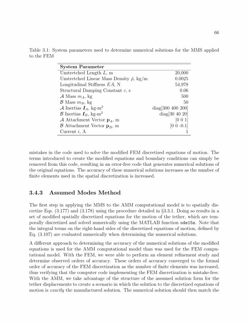
66

Table 3.1: System parameters used to determine numerical solutions for the MMS appliedto the FEM

System ParameterUnstretched Length L, m 20,000Unstretched Linear Mass Density ρ, kg/m 0.0025Longitudinal Stiffness EA, N 54,978Structural Damping Constant c, s 0.06A Mass mA, kg 500B Mass mB, kg 50A Inertias IA, kg-m2 diag[300 400 200]B Inertias IB, kg-m2 diag[30 40 20]A Attachment Vector pA, m [0 0 1]B Attachment Vector pB, m [0 0 -0.1]Current i, A 1

mistakes in the code used to solve the modified FEM discretized equations of motion. Theterms introduced to create the modified equations and boundary conditions can simply beremoved from this code, resulting in an error-free code that generates numerical solutions ofthe original equations. The accuracy of these numerical solutions increases as the number offinite elements used in the spatial discretization is increased.

3.4.3 Assumed Modes Method

The first step in applying the MMS to the AMM computational model is to spatially dis-cretize Eqs. (3.177) and (3.178) using the procedure detailed in §3.3.1. Doing so results in aset of modified spatially discretized equations for the motion of the tether, which are tem-porally discretized and solved numerically using the MATLAB function ode15s. Note thatthe integral terms on the right-hand sides of the discretized equations of motion, defined byEq. (3.107) are evaluated numerically when determining the numerical solutions.

A different approach to determining the accuracy of the numerical solutions of the modifiedequations is used for the AMM computational model than was used for the FEM compu-tational model. With the FEM, we were able to perform an element refinement study anddetermine observed orders of accuracy. These orders of accuracy converged to the formalorder of accuracy of the FEM discretization as the number of finite elements was increased,thus verifying that the computer code implementing the FEM discretization is mistake-free.With the AMM, we take advantage of the structure of the assumed solution form for thetether displacements to create a scenario in which the solution to the discretized equations ofmotion is exactly the manufactured solution. The numerical solution should then match the

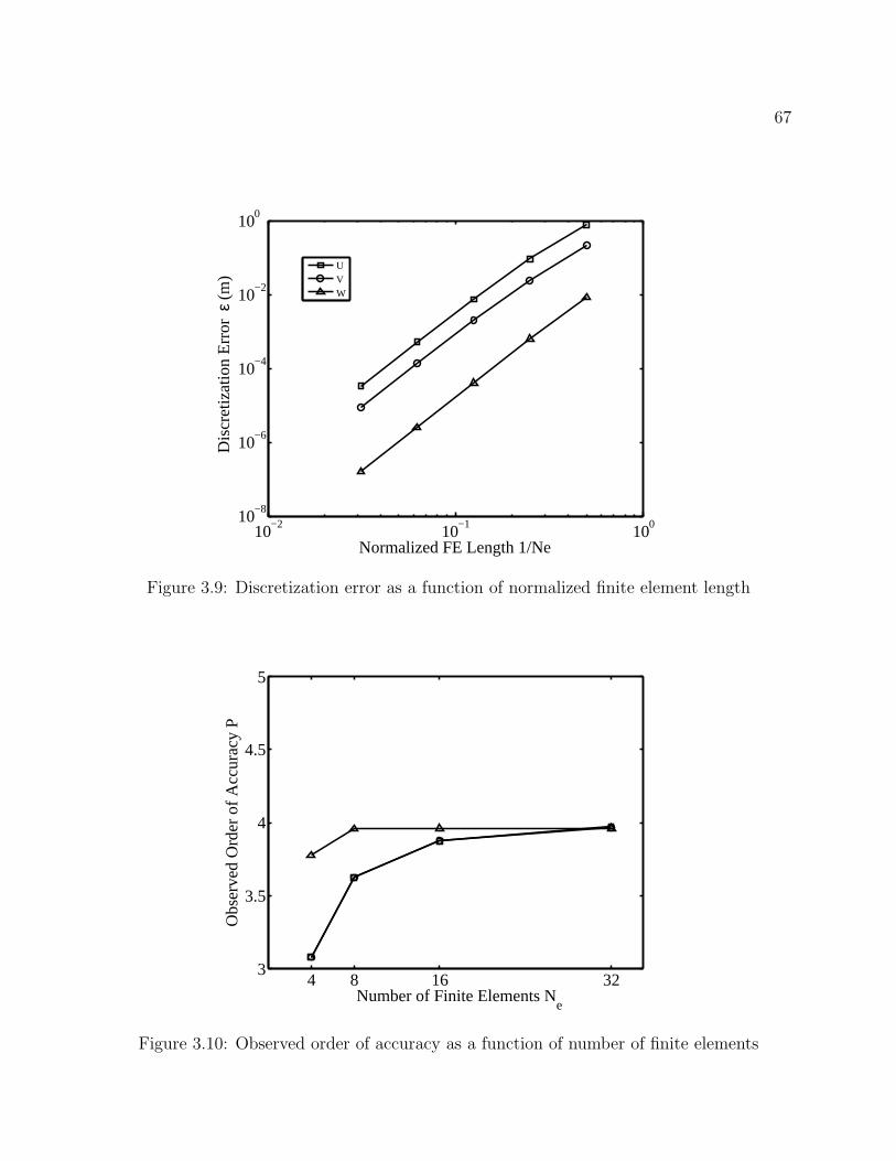
67

10−2

10−1

10010

−8

10−6

10−4

10−2

100

Normalized FE Length 1/Ne

Dis

cret

izat

ion

Err

or ε

(m)

UVW

Figure 3.9: Discretization error as a function of normalized finite element length

4 8 16 323

3.5

4

4.5

5

Number of Finite Elements Ne

Obs

erve

d O

rder

of

Acc

urac

y P

Figure 3.10: Observed order of accuracy as a function of number of finite elements

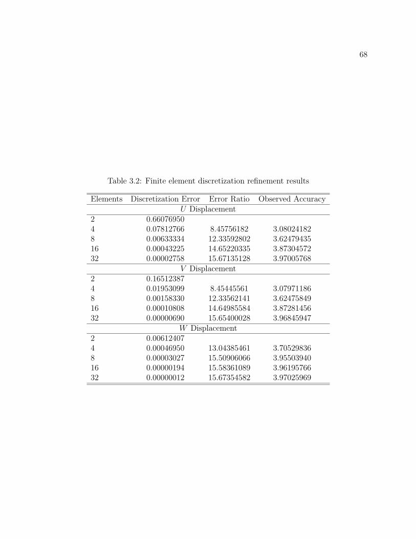
68

Table 3.2: Finite element discretization refinement results

Elements Discretization Error Error Ratio Observed AccuracyU Displacement

2 0.660769504 0.07812766 8.45756182 3.080241828 0.00633334 12.33592802 3.6247943516 0.00043225 14.65220335 3.8730457232 0.00002758 15.67135128 3.97005768

V Displacement2 0.165123874 0.01953099 8.45445561 3.079711868 0.00158330 12.33562141 3.6247584916 0.00010808 14.64985584 3.8728145632 0.00000690 15.65400028 3.96845947

W Displacement2 0.006124074 0.00046950 13.04385461 3.705298368 0.00003027 15.50906066 3.9550394016 0.00000194 15.58361089 3.9619576632 0.00000012 15.67354582 3.97025969

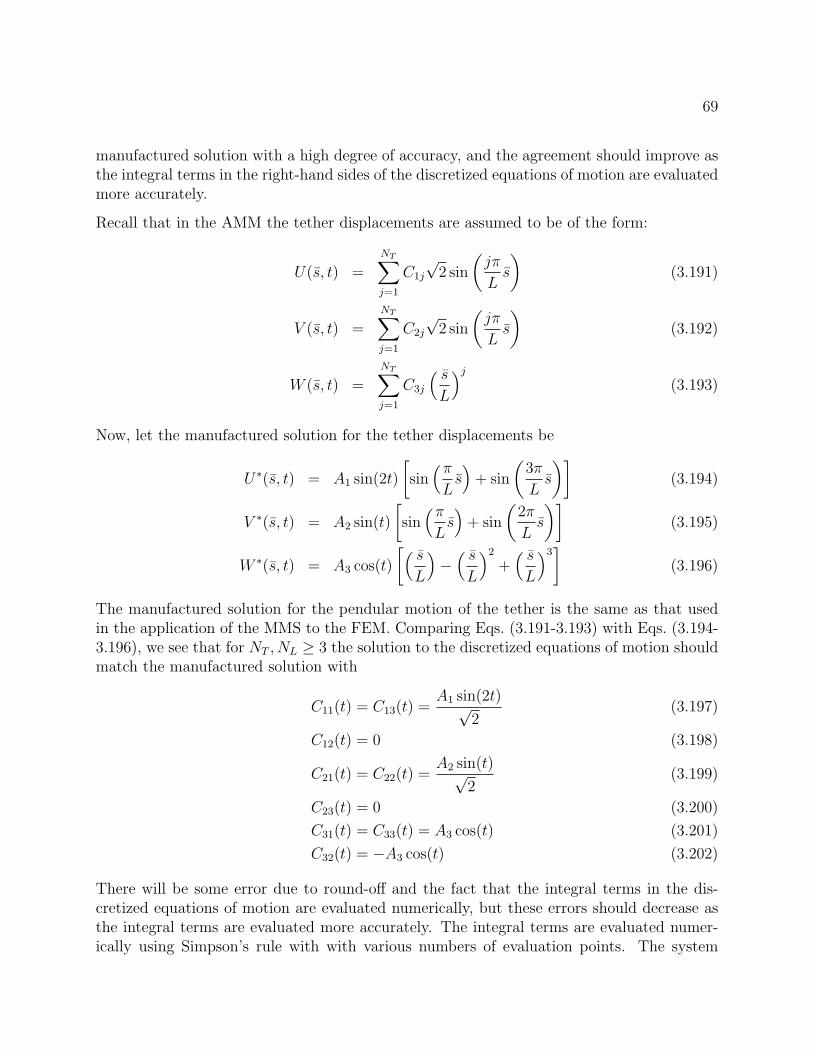
69

manufactured solution with a high degree of accuracy, and the agreement should improve asthe integral terms in the right-hand sides of the discretized equations of motion are evaluatedmore accurately.

Recall that in the AMM the tether displacements are assumed to be of the form:

U(s, t) =

NT∑j=1

C1j

√2 sin

(jπ

Ls

)(3.191)

V (s, t) =

NT∑j=1

C2j

√2 sin

(jπ

Ls

)(3.192)

W (s, t) =

NT∑j=1

C3j

( sL

)j(3.193)

Now, let the manufactured solution for the tether displacements be

U∗(s, t) = A1 sin(2t)

[sin(πLs)

+ sin

(3π

Ls

)](3.194)

V ∗(s, t) = A2 sin(t)

[sin(πLs)

+ sin

(2π

Ls

)](3.195)

W ∗(s, t) = A3 cos(t)

[( sL

)−( sL

)2

+( sL

)3]

(3.196)

The manufactured solution for the pendular motion of the tether is the same as that usedin the application of the MMS to the FEM. Comparing Eqs. (3.191-3.193) with Eqs. (3.194-3.196), we see that for NT , NL ≥ 3 the solution to the discretized equations of motion shouldmatch the manufactured solution with

C11(t) = C13(t) =A1 sin(2t)√

2(3.197)

C12(t) = 0 (3.198)

C21(t) = C22(t) =A2 sin(t)√

2(3.199)

C23(t) = 0 (3.200)

C31(t) = C33(t) = A3 cos(t) (3.201)

C32(t) = −A3 cos(t) (3.202)

There will be some error due to round-off and the fact that the integral terms in the dis-cretized equations of motion are evaluated numerically, but these errors should decrease asthe integral terms are evaluated more accurately. The integral terms are evaluated numer-ically using Simpson’s rule with with various numbers of evaluation points. The system

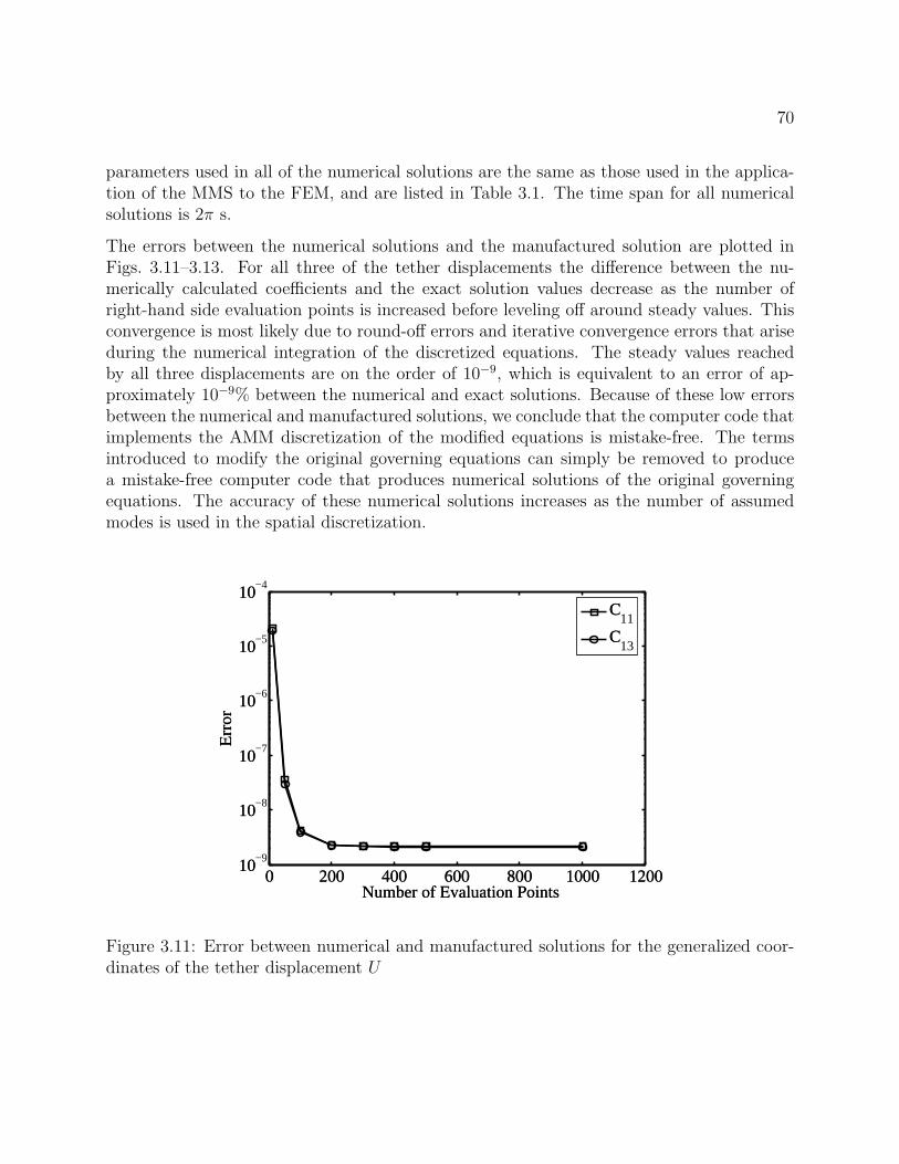
70

parameters used in all of the numerical solutions are the same as those used in the applica-tion of the MMS to the FEM, and are listed in Table 3.1. The time span for all numericalsolutions is 2π s.

The errors between the numerical solutions and the manufactured solution are plotted inFigs. 3.11–3.13. For all three of the tether displacements the difference between the nu-merically calculated coefficients and the exact solution values decrease as the number ofright-hand side evaluation points is increased before leveling off around steady values. Thisconvergence is most likely due to round-off errors and iterative convergence errors that ariseduring the numerical integration of the discretized equations. The steady values reachedby all three displacements are on the order of 10−9, which is equivalent to an error of ap-proximately 10−9% between the numerical and exact solutions. Because of these low errorsbetween the numerical and manufactured solutions, we conclude that the computer code thatimplements the AMM discretization of the modified equations is mistake-free. The termsintroduced to modify the original governing equations can simply be removed to producea mistake-free computer code that produces numerical solutions of the original governingequations. The accuracy of these numerical solutions increases as the number of assumedmodes is used in the spatial discretization.

0 200 400 600 800 1000 120010

−9

10−8

10−7

10−6

10−5

10−4

Number of Evaluation Points

Err

or

C

11

C13

Figure 3.11: Error between numerical and manufactured solutions for the generalized coor-dinates of the tether displacement U

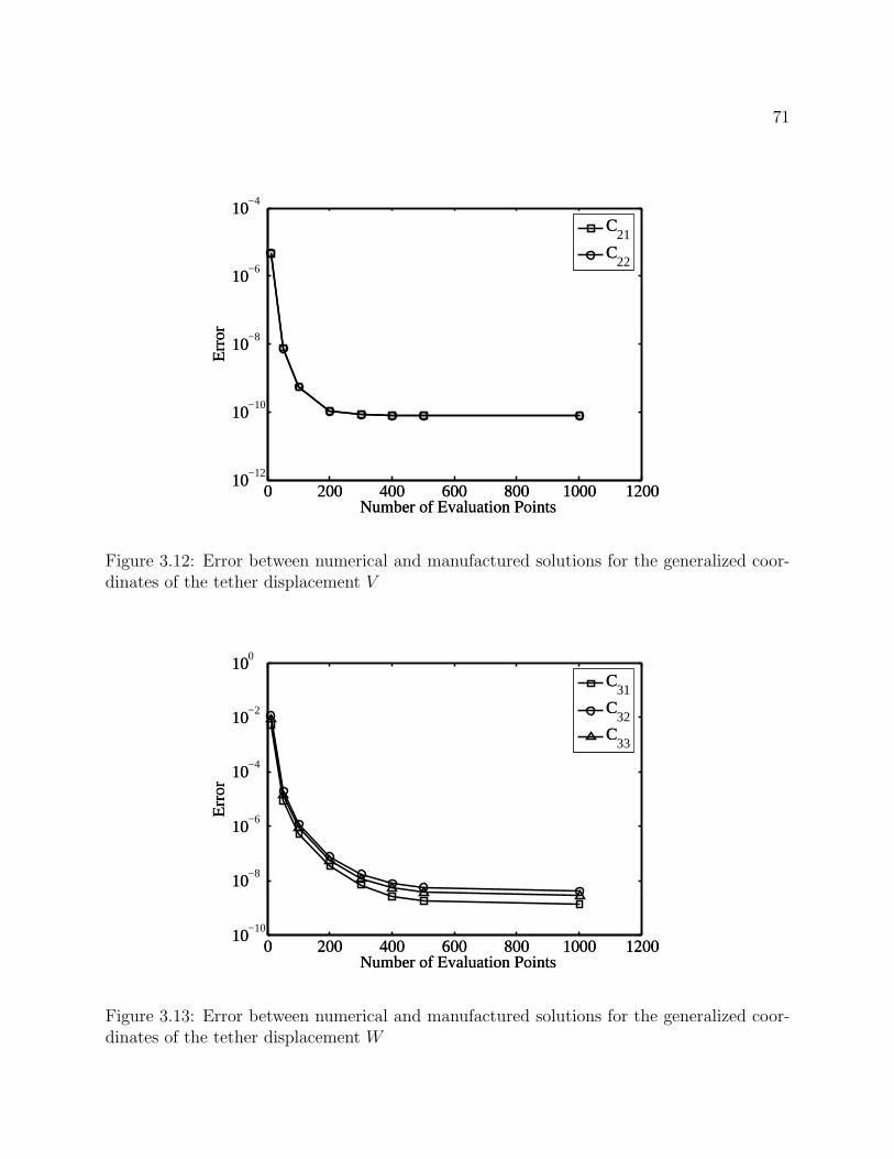
71

0 200 400 600 800 1000 120010

−12

10−10

10−8

10−6

10−4


Err

or

C

21

C22

Figure 3.12: Error between numerical and manufactured solutions for the generalized coor-dinates of the tether displacement V

0 200 400 600 800 1000 120010

−10

10−8

10−6

10−4

10−2

100


Err

or

C

31

C32

C33

Figure 3.13: Error between numerical and manufactured solutions for the generalized coor-dinates of the tether displacement W

72

3.5 Comparison of Computational Models

In the previous section we used the MMS to verify that the numerical solutions produced bythe computational models employing the AMM and FEM spatial discretizations are accuratesolutions of the mathematical model. From this analysis, we know that the numerical so-lutions produced by both computational models approach the solution of the mathematicalmodel as the spatial and temporal discretizations are refined. In this section, we present aqualitative comparison of the two computational models, with the objective of determiningwhich model is better suited for application to a TSS.

The most significant difference between the AMM and FEM computational models relates tothe computational time required for the models to produce numerical solutions. Numericalexperiments have shown that both computational models work well for low numbers of as-sumed modes or finite elements, in that both produce numerical solutions in a relatively shortcomputational time. However, as the number of assumed modes used in the AMM compu-tational model to approximate the longitudinal vibrations increases, the computational timeincreases rapidly, rendering the model practically useless. To see why this happens, considerthe mass matrix of the discretized equations for the longitudinal vibrations, which is definedby Eq. (3.116). As NL increases, the columns of the longitudinal mass matrix become in-creasingly similar, causing the mass matrix to become nearly singular. This nearly-singularbehavior introduces significant numerical errors into the calculation of the accelerations ofthe longitudinal degrees of freedom because the inverse of the mass matrix is used in theircalculations, and these errors in the accelerations can actually cause the longitudinal vibra-tions to diverge when they should not. As the time integrator attempts to compensate forthis divergent behavior, the time steps become very small and the total integration timebecomes prohibitively large. The FEM does not have this same problem because the diag-onal structure of the system mass matrices ensures that their columns are always linearlyindependent, so there are no problems in taking their inverses due to ill-conditioning.

Nearly singular behavior of the system mass matrix for simple polynomial shape functionsin the AMM has been reported previously,57 and the simplest method of eliminating theproblem is to use a different set of assumed mode functions for the longitudinal vibrations.The best possible set is an orthogonal set that makes the mass matrix diagonal and triviallyinvertible. Another possibility is to use the mode shapes for the longitudinal vibrationsof a similar, but much simpler, problem as the longitudinal assumed mode functions. Forexample, one could use the longitudinal mode shapes for a simple string pendulum as thelongitudinal modes shapes for the TSS. The mode shapes of the simpler problem would beorthogonal or nearly orthogonal, and the resulting mass matrix would always have a well-defined inverse. Other possible sets of longitudinal assumed mode functions exist, but theiranalysis and implementation is left for future work.

Another advantage of the FEM over the AMM not specific to the shape functions used inthe AMM is that initial conditions are much easier to set in the FEM. Since the degrees

73

of freedom in the FEM are simply displacements and slopes at points along the tether,any arbitrary initial tether shape can be trivially converted to a set of initial coordinatesfor numerical integration. This is not the case with the AMM, in which determining a setof coordinates from an arbitrary tether shape requires a process similar to calculating thecoefficients of a Fourier series. While this is not necessarily a difficult task, it is more involvedthan the process required in the FEM.

For the reasons discussed above, we conclude that the FEM computational model is bettersuited for application to the TSS than is the AMM computational model. All applicationsof the top-level computational model presented later in this dissertation use the FEM com-putational model, so from this point forward the phrase “top-level computational model”refers to the FEM computational model presented in this chapter. In the next section, wepresent the outputs of the top-level computational model for two different applications of aTSS, along with a discussion of the various aspects of the system dynamics.

3.6 Examples of Computational Model Output

In this section we present examples of the output of the top-level computational model fortwo different TSS. The first system is a spinning, non-electrodynamic TSS, and the secondsystem is a local-vertically aligned electrodynamic TSS. The top-level computational modelis used to produce numerical solutions for both examples, and we present and discuss thenumerical solutions for both systems.

3.6.1 Example 1: Spinning Tethered Satellite System

The first example that we consider is for a spinning, non-electrodynamic TSS. The systemparameters used in this example are listed in Table 3.3, and the initial conditions used toproduce the numerical solution are listed in Table 3.4. Note that 4 finite elements are usedin the spatial discretization, and the time span of the numerical solution is approximately5 orbits of the system. The initial conditions correspond to the system being on a nearlycircular orbit with an altitude of roughly 400 km. The entire system is nominally spinningin the orbit plane at roughly 5 times per orbit, but there is a small initial out-of-plane tetherattitude angle of 1. The tether initially has sinusoidal transverse displacements (both U andV ) with maximum displacement of 20 m, and the initial longitudinal displacement profile iscubic. Note that this cubic displacement profile is determined using a quadratic expressionfor the tension in the tether, as in Ref. [5].

The time history of the osculating orbit elements predicted by the top-level computationalmodel is shown in Fig. 3.14. Note that the osculating orbit elements (and all of the otherquantities presented for the examples considered in this section) are plotted against a nondi-mensional time, which is defined as the dimensional time divided by the orbital period of the

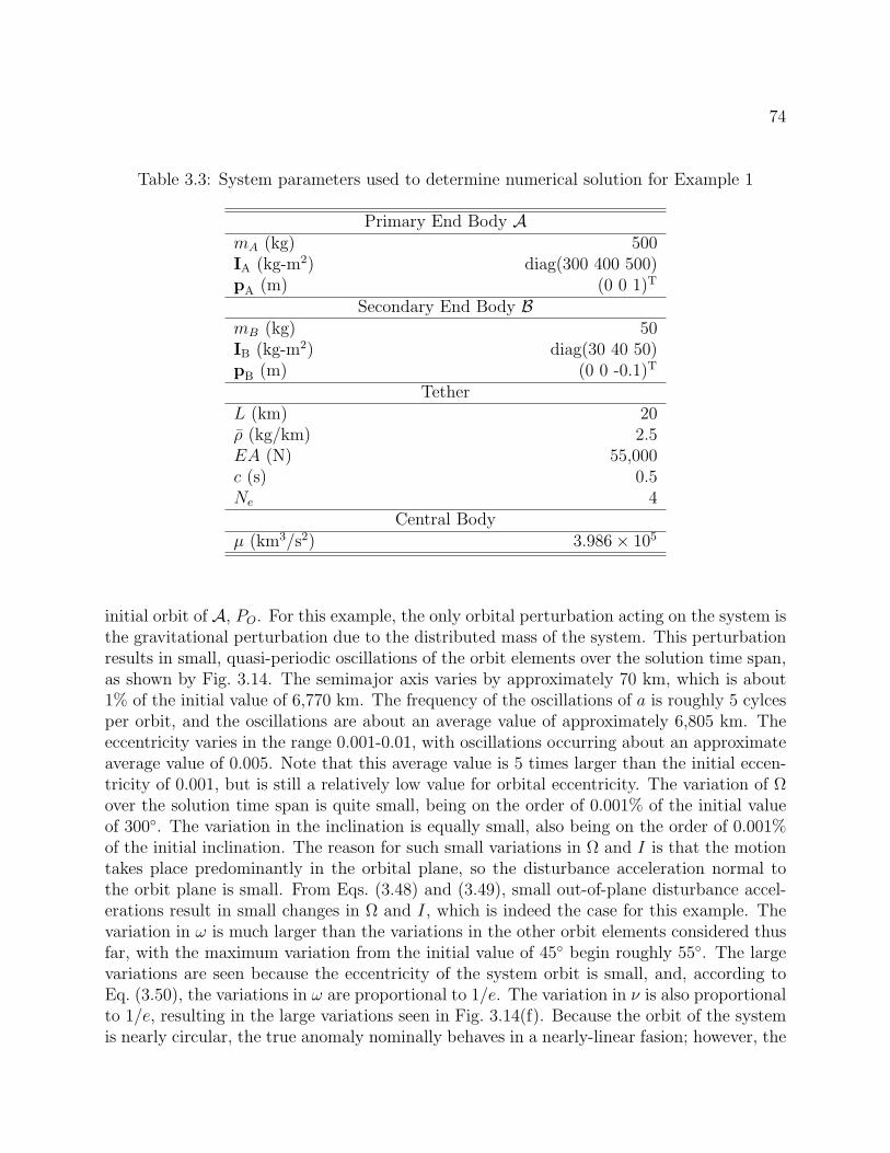
74

Table 3.3: System parameters used to determine numerical solution for Example 1

Primary End Body AmA (kg) 500IA (kg-m2) diag(300 400 500)pA (m) (0 0 1)T

Secondary End Body BmB (kg) 50IB (kg-m2) diag(30 40 50)pB (m) (0 0 -0.1)T

TetherL (km) 20ρ (kg/km) 2.5EA (N) 55,000c (s) 0.5Ne 4

Central Bodyµ (km3/s2) 3.986× 105

initial orbit of A, PO. For this example, the only orbital perturbation acting on the system isthe gravitational perturbation due to the distributed mass of the system. This perturbationresults in small, quasi-periodic oscillations of the orbit elements over the solution time span,as shown by Fig. 3.14. The semimajor axis varies by approximately 70 km, which is about1% of the initial value of 6,770 km. The frequency of the oscillations of a is roughly 5 cylcesper orbit, and the oscillations are about an average value of approximately 6,805 km. Theeccentricity varies in the range 0.001-0.01, with oscillations occurring about an approximateaverage value of 0.005. Note that this average value is 5 times larger than the initial eccen-tricity of 0.001, but is still a relatively low value for orbital eccentricity. The variation of Ωover the solution time span is quite small, being on the order of 0.001% of the initial valueof 300. The variation in the inclination is equally small, also being on the order of 0.001%of the initial inclination. The reason for such small variations in Ω and I is that the motiontakes place predominantly in the orbital plane, so the disturbance acceleration normal tothe orbit plane is small. From Eqs. (3.48) and (3.49), small out-of-plane disturbance accel-erations result in small changes in Ω and I, which is indeed the case for this example. Thevariation in ω is much larger than the variations in the other orbit elements considered thusfar, with the maximum variation from the initial value of 45 begin roughly 55. The largevariations are seen because the eccentricity of the system orbit is small, and, according toEq. (3.50), the variations in ω are proportional to 1/e. The variation in ν is also proportionalto 1/e, resulting in the large variations seen in Fig. 3.14(f). Because the orbit of the systemis nearly circular, the true anomaly nominally behaves in a nearly-linear fasion; however, the

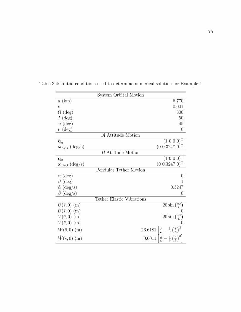
75

Table 3.4: Initial conditions used to determine numerical solution for Example 1

System Orbital Motiona (km) 6,770e 0.001Ω (deg) 300I (deg) 50ω (deg) 45ν (deg) 0

A Attitude MotionqA (1 0 0 0)T

ωA/O (deg/s) (0 0.3247 0)T

B Attitude MotionqB (1 0 0 0)T

ωB/O (deg/s) (0 0.3247 0)T

Pendular Tether Motionα (deg) 0β (deg) 1α (deg/s) 0.3247

β (deg/s) 0Tether Elastic Vibrations

U(s, 0) (m) 20 sin(πsL

)U(s, 0) (m) 0V (s, 0) (m) 20 sin

(πsL

)V (s, 0) (m) 0

W (s, 0) (m) 26.6181[sL− 1

9

(sL

)3]

W (s, 0) (m) 0.0011[sL− 1

9

(sL

)3]

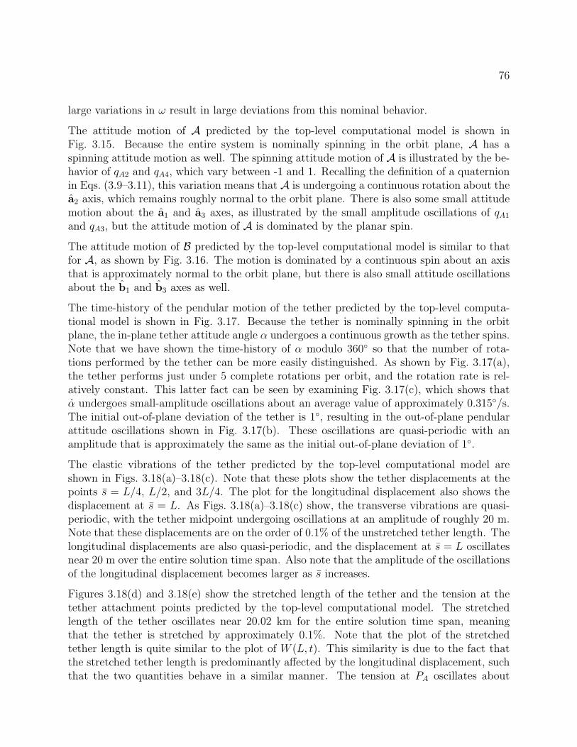
76

large variations in ω result in large deviations from this nominal behavior.

The attitude motion of A predicted by the top-level computational model is shown inFig. 3.15. Because the entire system is nominally spinning in the orbit plane, A has aspinning attitude motion as well. The spinning attitude motion of A is illustrated by the be-havior of qA2 and qA4, which vary between -1 and 1. Recalling the definition of a quaternionin Eqs. (3.9–3.11), this variation means that A is undergoing a continuous rotation about thea2 axis, which remains roughly normal to the orbit plane. There is also some small attitudemotion about the a1 and a3 axes, as illustrated by the small amplitude oscillations of qA1

and qA3, but the attitude motion of A is dominated by the planar spin.

The attitude motion of B predicted by the top-level computational model is similar to thatfor A, as shown by Fig. 3.16. The motion is dominated by a continuous spin about an axisthat is approximately normal to the orbit plane, but there is also small attitude oscillationsabout the b1 and b3 axes as well.

The time-history of the pendular motion of the tether predicted by the top-level computa-tional model is shown in Fig. 3.17. Because the tether is nominally spinning in the orbitplane, the in-plane tether attitude angle α undergoes a continuous growth as the tether spins.Note that we have shown the time-history of α modulo 360 so that the number of rota-tions performed by the tether can be more easily distinguished. As shown by Fig. 3.17(a),the tether performs just under 5 complete rotations per orbit, and the rotation rate is rel-atively constant. This latter fact can be seen by examining Fig. 3.17(c), which shows thatα undergoes small-amplitude oscillations about an average value of approximately 0.315/s.The initial out-of-plane deviation of the tether is 1, resulting in the out-of-plane pendularattitude oscillations shown in Fig. 3.17(b). These oscillations are quasi-periodic with anamplitude that is approximately the same as the initial out-of-plane deviation of 1.

The elastic vibrations of the tether predicted by the top-level computational model areshown in Figs. 3.18(a)–3.18(c). Note that these plots show the tether displacements at thepoints s = L/4, L/2, and 3L/4. The plot for the longitudinal displacement also shows thedisplacement at s = L. As Figs. 3.18(a)–3.18(c) show, the transverse vibrations are quasi-periodic, with the tether midpoint undergoing oscillations at an amplitude of roughly 20 m.Note that these displacements are on the order of 0.1% of the unstretched tether length. Thelongitudinal displacements are also quasi-periodic, and the displacement at s = L oscillatesnear 20 m over the entire solution time span. Also note that the amplitude of the oscillationsof the longitudinal displacement becomes larger as s increases.

Figures 3.18(d) and 3.18(e) show the stretched length of the tether and the tension at thetether attachment points predicted by the top-level computational model. The stretchedlength of the tether oscillates near 20.02 km for the entire solution time span, meaningthat the tether is stretched by approximately 0.1%. Note that the plot of the stretchedtether length is quite similar to the plot of W (L, t). This similarity is due to the fact thatthe stretched tether length is predominantly affected by the longitudinal displacement, suchthat the two quantities behave in a similar manner. The tension at PA oscillates about

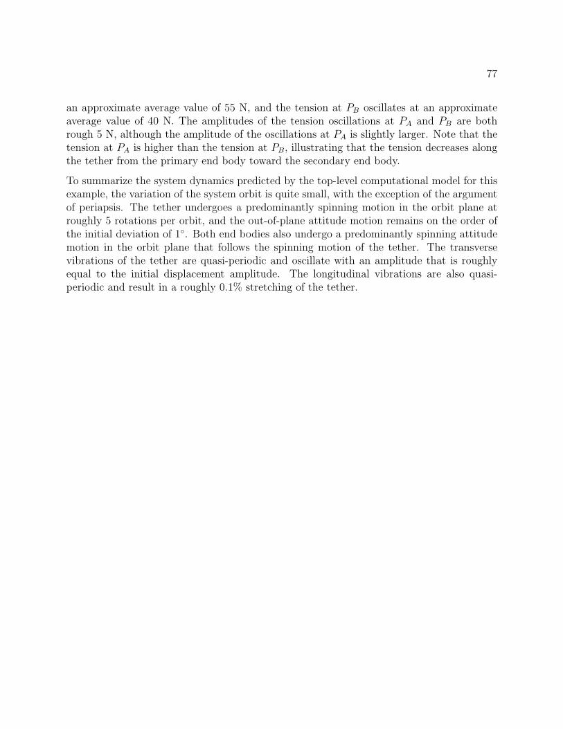
77

an approximate average value of 55 N, and the tension at PB oscillates at an approximateaverage value of 40 N. The amplitudes of the tension oscillations at PA and PB are bothrough 5 N, although the amplitude of the oscillations at PA is slightly larger. Note that thetension at PA is higher than the tension at PB, illustrating that the tension decreases alongthe tether from the primary end body toward the secondary end body.

To summarize the system dynamics predicted by the top-level computational model for thisexample, the variation of the system orbit is quite small, with the exception of the argumentof periapsis. The tether undergoes a predominantly spinning motion in the orbit plane atroughly 5 rotations per orbit, and the out-of-plane attitude motion remains on the order ofthe initial deviation of 1. Both end bodies also undergo a predominantly spinning attitudemotion in the orbit plane that follows the spinning motion of the tether. The transversevibrations of the tether are quasi-periodic and oscillate with an amplitude that is roughlyequal to the initial displacement amplitude. The longitudinal vibrations are also quasi-periodic and result in a roughly 0.1% stretching of the tether.

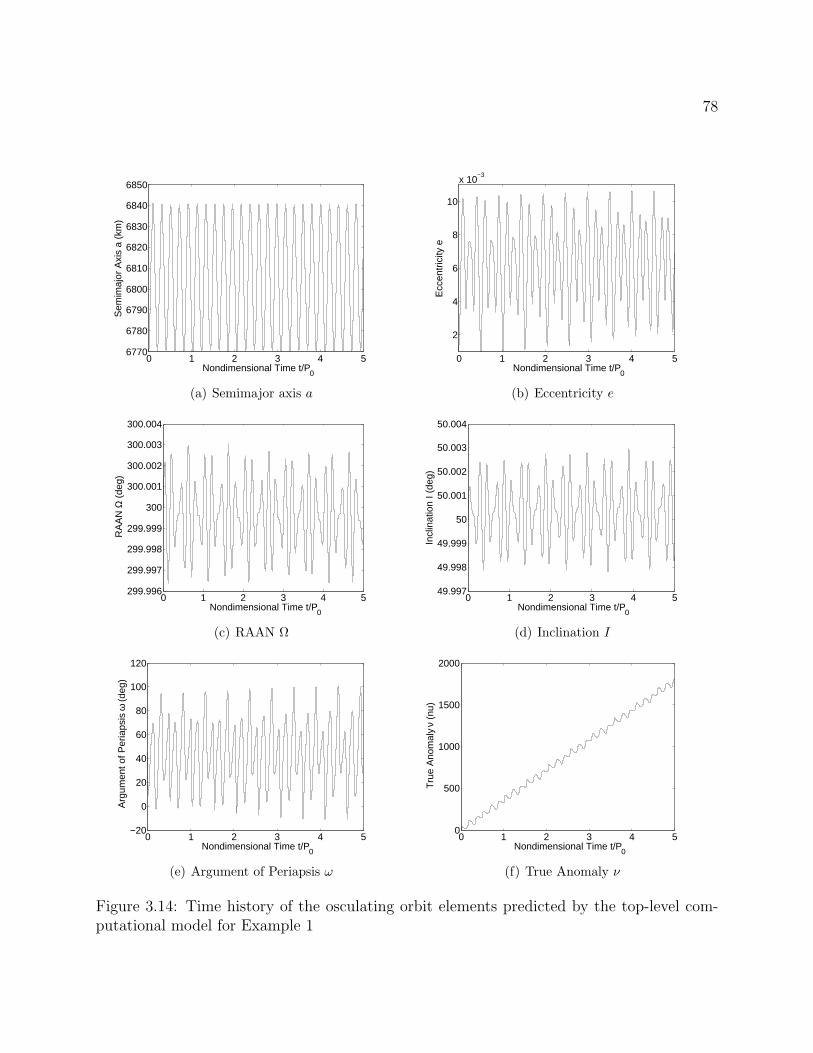
78

0 1 2 3 4 56770

6780

6790

6800

6810

6820

6830

6840

6850

Nondimensional Time t/P0

Sem

imaj

or A

xis

a (k

m)

(a) Semimajor axis a

0 1 2 3 4 5

2

4

6

8

10

x 10−3


Ecc

entr

icity

e

(b) Eccentricity e

0 1 2 3 4 5299.996

299.997

299.998

299.999

300

300.001

300.002

300.003

300.004


RA

AN

Ω (

deg)

(c) RAAN Ω

0 1 2 3 4 549.997

49.998

49.999

50

50.001

50.002

50.003

50.004


Incl

inat

ion

I (de

g)

(d) Inclination I

0 1 2 3 4 5−20

0

20

40

60

80

100

120


Arg

umen

t of P

eria

psis

ω (

deg)

(e) Argument of Periapsis ω

0 1 2 3 4 50

500

1000

1500

2000


Tru

e A

nom

aly

ν (n

u)

(f) True Anomaly ν

Figure 3.14: Time history of the osculating orbit elements predicted by the top-level com-putational model for Example 1

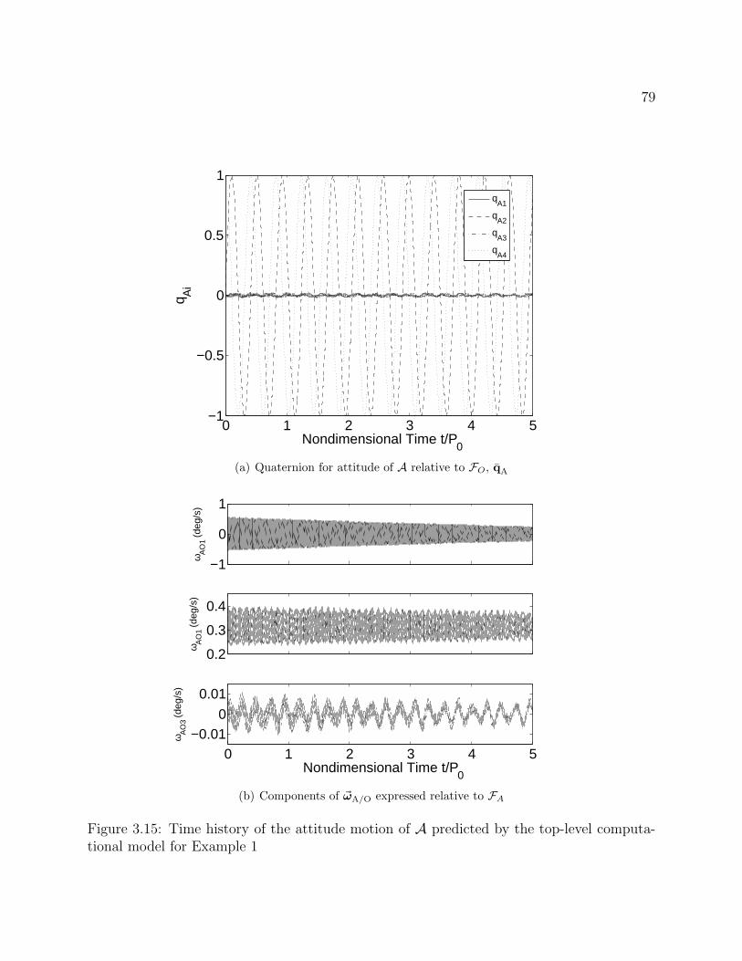
79

0 1 2 3 4 5−1

−0.5

0

0.5

1


q Ai

qA1

qA2

qA3

qA4

(a) Quaternion for attitude of A relative to FO, qA

−1

0

1

ω AO

1 (de

g/s)

0.2

0.3

0.4

ω AO

1 (de

g/s)

0 1 2 3 4 5−0.01

0

0.01


ω AO

3 (de

g/s)

(b) Components of ~ωA/O expressed relative to FA

Figure 3.15: Time history of the attitude motion of A predicted by the top-level computa-tional model for Example 1

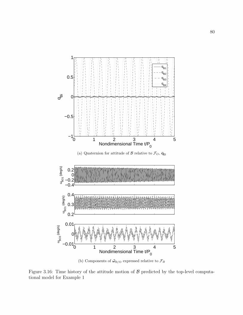
80

0 1 2 3 4 5−1

−0.5

0

0.5

1


q Bi

qB1

qB2

qB3

qB4

(a) Quaternion for attitude of B relative to FO, qB

−0.4−0.2

00.2

ω BO

1 (de

g/s)

0.2

0.3

0.4

ω BO

1 (de

g/s)

0 1 2 3 4 5−0.01

0

0.01


ω BO

3 (de

g/s)

(b) Components of ~ωB/O expressed relative to FB

Figure 3.16: Time history of the attitude motion of B predicted by the top-level computa-tional model for Example 1

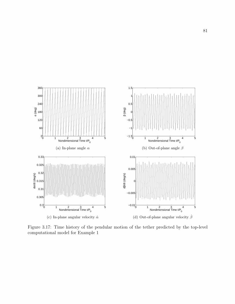
81

0 1 2 3 4 50

60

120

180

240

300

360


α (d

eg)

(a) In-plane angle α

0 1 2 3 4 5−1.5

−1

−0.5

0

0.5

1

1.5


β (d

eg)

(b) Out-of-plane angle β

0 1 2 3 4 50.3

0.305

0.31

0.315

0.32

0.325

0.33


dα/d

t (de

g/s)

(c) In-plane angular velocity α

0 1 2 3 4 5−0.01

−0.005

0

0.005

0.01


dβ/d

t (de

g/s)

(d) Out-of-plane angular velocity β

Figure 3.17: Time history of the pendular motion of the tether predicted by the top-levelcomputational model for Example 1

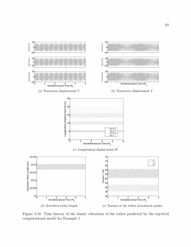
82

−20

0

20

U(L

/4,t)

(m

)

−20

0

20

U(L

/2,t)

(m

)

0 1 2 3 4 5−20

0

20

U(3

L/4,

t) (

m)


(a) Transverse displacement U

−20

0

20

V(L

/4,t)

(m

)

−20

0

20

V(L

/2,t)

(m

)

−20

0

20

V(3

L/4,

t) (

m)


(b) Transverse displacement V

0 1 2 3 4 50

5

10

15

20

25


Long

itudi

nal D

ispl

acem

ent W

(m

)

W(L/4,t)W(L/2,t)W(3L/4,t)W(L,t)

(c) Longitudinal displacement W

0 1 2 3 4 520

20.005

20.01

20.015

20.02

20.025


Str

etch

ed T

ethe

r Le

ngth

(km

)

(d) Stretched tether length

0 1 2 3 4 530

35

40

45

50

55

60

65

70

75


Ten

sion

T (

N)

PA

PB

(e) Tension at the tether attachment points

Figure 3.18: Time history of the elastic vibrations of the tether predicted by the top-levelcomputational model for Example 1

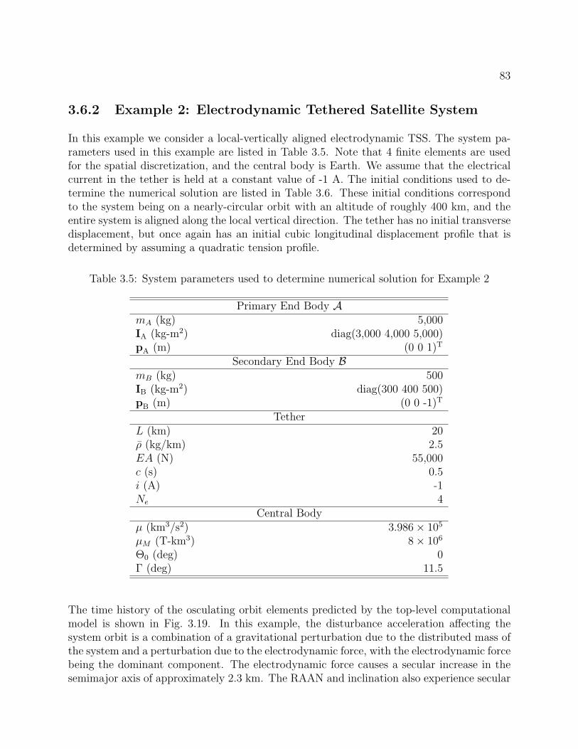
83

3.6.2 Example 2: Electrodynamic Tethered Satellite System

In this example we consider a local-vertically aligned electrodynamic TSS. The system pa-rameters used in this example are listed in Table 3.5. Note that 4 finite elements are usedfor the spatial discretization, and the central body is Earth. We assume that the electricalcurrent in the tether is held at a constant value of -1 A. The initial conditions used to de-termine the numerical solution are listed in Table 3.6. These initial conditions correspondto the system being on a nearly-circular orbit with an altitude of roughly 400 km, and theentire system is aligned along the local vertical direction. The tether has no initial transversedisplacement, but once again has an initial cubic longitudinal displacement profile that isdetermined by assuming a quadratic tension profile.

Table 3.5: System parameters used to determine numerical solution for Example 2

Primary End Body AmA (kg) 5,000IA (kg-m2) diag(3,000 4,000 5,000)pA (m) (0 0 1)T

Secondary End Body BmB (kg) 500IB (kg-m2) diag(300 400 500)pB (m) (0 0 -1)T

TetherL (km) 20ρ (kg/km) 2.5EA (N) 55,000c (s) 0.5i (A) -1Ne 4


µM (T-km3) 8× 106

Θ0 (deg) 0Γ (deg) 11.5

The time history of the osculating orbit elements predicted by the top-level computationalmodel is shown in Fig. 3.19. In this example, the disturbance acceleration affecting thesystem orbit is a combination of a gravitational perturbation due to the distributed mass ofthe system and a perturbation due to the electrodynamic force, with the electrodynamic forcebeing the dominant component. The electrodynamic force causes a secular increase in thesemimajor axis of approximately 2.3 km. The RAAN and inclination also experience secular

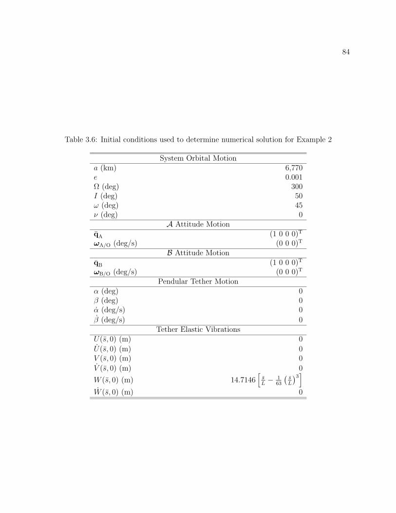
84

Table 3.6: Initial conditions used to determine numerical solution for Example 2



ωA/O (deg/s) (0 0 0)T


ωB/O (deg/s) (0 0 0)T

Pendular Tether Motionα (deg) 0β (deg) 0α (deg/s) 0


U(s, 0) (m) 0

U(s, 0) (m) 0V (s, 0) (m) 0

V (s, 0) (m) 0

W (s, 0) (m) 14.7146[sL− 1

63

(sL

)3]

W (s, 0) (m) 0

85

drifts due to the electrodynamic force, with both quantities decreasing over the solutiontime span. Note, however, that the decrease in both quantities is quite small compared totheir initial values. The eccentricity and argument of periapsis do not appear to exhibit anysecular drift, and instead undergo quasi-periodic oscillations about an average value. Forthe eccentricity, the average value is roughly 0.00175, and the amplitude of the oscillationsis about 0.00075. The average value of ω is approximately the initial value of 45, and theamplitude of the oscillations is about 25. Both e and ω oscillate at approximately 5 cyclesper orbit. The true anomaly increases continuously as expected, with some variations dueto the variation in the argument of periapsis.

Figure 3.20 shows the time history of the attitude motion of A. The principal axes of A areinitially aligned with FO, and, as the figure shows, undergoes small amplitude oscillationsabout this initial orientation. This behavior is illustrated by the fact that qA4 is approx-imately 1 over the entire solution time span, while the other qAi remain near zero. Theattitude motion of B is similar to that of A, as shown by Fig. 3.21. The principal axes ofB are initially aligned with FO, and the body undergoes small amplitude oscillations aboutthe initial orientation over the solution time span.

The time history of the pendular tether motion predicted by the top-level computationalmodel is shown in Fig. 3.22. The tether is initially aligned with the local vertical direction,and the electrodynamic force drives small amplitude in- and out-of-plane tether attitudemotion. The maximum magnitude of both the in- and out-of-plane tether attitude angles is0.45. Note that the out-of-plane attitude angle behaves in a much more periodic mannerthan does the in-plane angle, which appears to be oscillating in a somewhat chaotic manner.

The tether elastic vibrations predicted by the top-level computational model are shown inFigs. 3.23(a)–3.23(c). As with the first example we considered, the elastic vibrations areillustrated by displaying the tether displacements at several points along the tether. Thetether is initially aligned with the local vertical with some longitudinal stretching, and theelectrodynamic force drives transverse vibrations of the tether. As Fig. 3.23(a) shows, thedisplacement u undergoes quasi-periodic oscillations. Note that U at all of the points shownis positive because the component of the electrodynamic force in the e1 direction is alwayspositive for this example, thus driving the positive oscillations seen in Fig. 3.23(a). Thesame cannot be said for the displacement V , however, as seen by Fig. 3.23(b). The behaviorof V appears to be a combination of oscillations at a high frequency and oscillations at a lowfrequency. The high frequency is simply the natural oscillation frequency of the tether, andthe low frequency is due to the fact that the component of the electrodynamic force in thee2 direction slowly changes as the system moves in its inclined orbit. This force componentslowly oscillates back and forth between positive and negative quantities at a frequencyslightly lower that the orbital frequency (due to the rotation of the magnetic field), resultingin the alternately positive and negative character of V seen in Fig. 3.23(b). The combinationof the behaviors of U and V results is a sort of slowly-varying “skip-rope” motion of thetether as seen by the frame FE. The tether longitudinal vibrations behave much in thesame manner as seen in the first example we considered. As illustrated by Fig. 3.23(c),

86

the longitudinal stretching of the tether remains relatively constant, with a longitudinaldisplacement at s = L of approximately 13 m. Another point to note about Fig. 3.23(c)is that the longitudinal displacement undergoes a period of high-frequency oscillation atthe beginning of the motion that damps out within a fraction of an orbit. This behaviorillustrates the primary affect of the structural damping in the tether, which is to damp outhigh-frequency longitudinal vibrations.

The stretched tether length and tension at the tether attachment points predicted by thetop-level computational model are shown in Figs. 3.23(d)–3.23(e). The stretched length ofthe tether undergoes a short period of high-frequency oscillations that damp out around avalue of roughly 20.013 km, meaning that the tether is stretched by 0.065%. As discussedin the previous example, the behavior of the stretched tether length closely resembles thebehavior of the longitudinal vibrations. The tension at PA oscillates about an average valueslightly larger than 36 N, and the tension at PB oscillates about an average value near 35 N.As seen in the first example we considered, the tension in the tether decreases as s increasesfrom PA to PB.

To summarize the system dynamics predicted by the top-level computational model for thisexample, the electrodynamic force causes secular changes in the semimajor axis, RAAN, andinclination of the system orbit. The change in the semimajor axis is relatively significant,while the changes in the RAAN and inclination are practically negligible. The principal axesof both end bodies are initially aligned with the orbital frame and undergo small amplitudeattitude oscillations about this initial configuration. The electrodynamic force drives smallamplitude in- and out-of-plane pendular tether motion, with the maximum magnitude ofboth in- and out-of-plane motion being roughly 0.45. The transverse vibrations inducedby the electrodynamic force are relatively complex, exhibiting a “skip-rope” type of motion.The longitudinal vibrations are similar to those seen in the first example we considered, inthat they remain at relatively constant values over the solution time span.

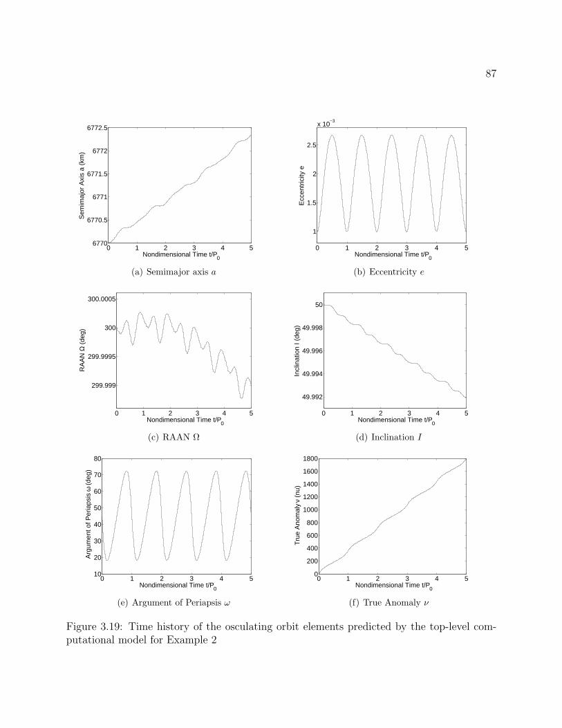
87

0 1 2 3 4 56770

6770.5

6771

6771.5

6772

6772.5


Sem

imaj

or A

xis

a (k

m)

(a) Semimajor axis a

0 1 2 3 4 5

1

1.5

2

2.5

x 10−3


Ecc

entr

icity

e

(b) Eccentricity e

0 1 2 3 4 5

299.999

299.9995

300

300.0005


RA

AN

Ω (

deg)

(c) RAAN Ω

0 1 2 3 4 5

49.992

49.994

49.996

49.998

50


Incl

inat

ion

I (de

g)

(d) Inclination I

0 1 2 3 4 510

20

30

40

50

60

70

80


Arg

umen

t of P

eria

psis

ω (

deg)

(e) Argument of Periapsis ω

0 1 2 3 4 50

200

400

600

800

1000

1200

1400

1600

1800


Tru

e A

nom

aly

ν (n

u)

(f) True Anomaly ν

Figure 3.19: Time history of the osculating orbit elements predicted by the top-level com-putational model for Example 2

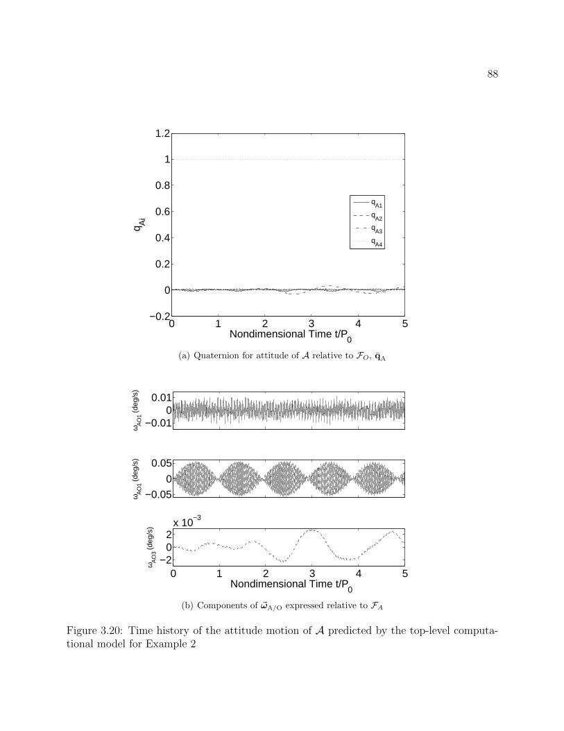
88

0 1 2 3 4 5−0.2

0

0.2

0.4

0.6

0.8

1

1.2


q Ai

qA1

qA2

qA3

qA4

(a) Quaternion for attitude of A relative to FO, qA

−0.010

0.01

ω AO

1 (de

g/s)

−0.05

0

0.05

ω AO

1 (de

g/s)

0 1 2 3 4 5−2

02

x 10−3


ω AO

3 (de

g/s)

(b) Components of ~ωA/O expressed relative to FA

Figure 3.20: Time history of the attitude motion of A predicted by the top-level computa-tional model for Example 2

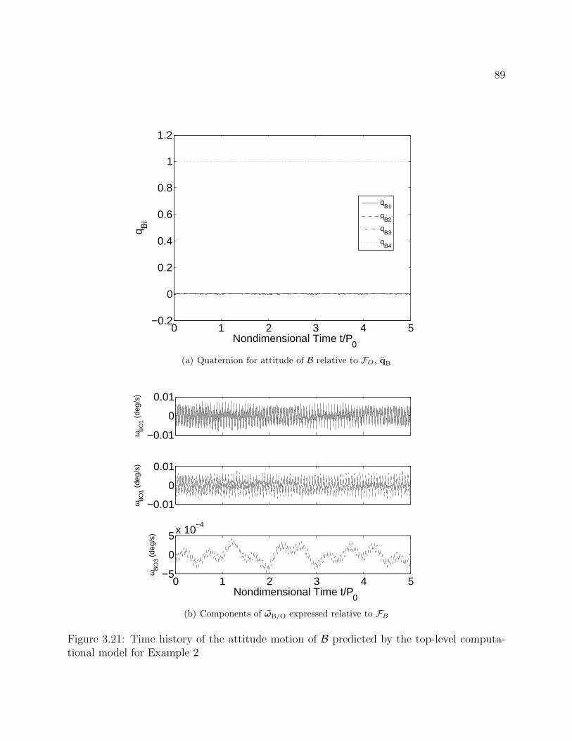
89

0 1 2 3 4 5−0.2

0

0.2

0.4

0.6

0.8

1

1.2


q Bi

qB1

qB2

qB3

qB4

(a) Quaternion for attitude of B relative to FO, qB

−0.01

0

0.01

ω BO

1 (de

g/s)

−0.01

0

0.01

ω BO

1 (de

g/s)

0 1 2 3 4 5−5

0

5x 10−4


ω BO

3 (de

g/s)

(b) Components of ~ωB/O expressed relative to FB

Figure 3.21: Time history of the attitude motion of B predicted by the top-level computa-tional model for Example 2

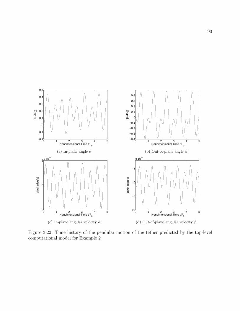
90

0 1 2 3 4 5−0.2

−0.1

0

0.1

0.2

0.3

0.4

0.5


α (d

eg)

(a) In-plane angle α

0 1 2 3 4 5−0.4

−0.3

−0.2

−0.1

0

0.1

0.2

0.3

0.4


β (d

eg)

(b) Out-of-plane angle β

0 1 2 3 4 5−5

0

5x 10−4


dα/d

t (de

g/s)

(c) In-plane angular velocity α

0 1 2 3 4 5−10

−5

0

5

x 10−4


dβ/d

t (de

g/s)

(d) Out-of-plane angular velocity β

Figure 3.22: Time history of the pendular motion of the tether predicted by the top-levelcomputational model for Example 2

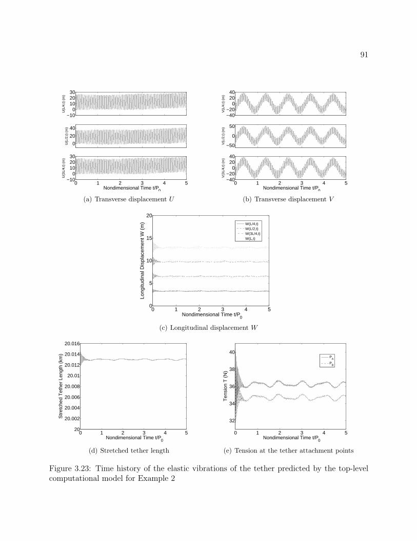
91

−100

102030

U(L

/4,t)

(m

)

0

20

40

U(L

/2,t)

(m

)

0 1 2 3 4 5−10

0102030

U(3

L/4,

t) (

m)


(a) Transverse displacement U

−40−20

02040

V(L

/4,t)

(m

)

−50

0

50

V(L

/2,t)

(m

)

0 1 2 3 4 5−40−20

02040

V(3

L/4,

t) (

m)


(b) Transverse displacement V

0 1 2 3 4 50

5

10

15

20


Long

itudi

nal D

ispl

acem

ent W

(m

)

W(L/4,t)W(L/2,t)W(3L/4,t)W(L,t)

(c) Longitudinal displacement W

0 1 2 3 4 520

20.002

20.004

20.006

20.008

20.01

20.012

20.014

20.016


Str

etch

ed T

ethe

r Le

ngth

(km

)

(d) Stretched tether length

0 1 2 3 4 5

32

34

36

38

40


Ten

sion

T (

N)

PA

PB

(e) Tension at the tether attachment points

Figure 3.23: Time history of the elastic vibrations of the tether predicted by the top-levelcomputational model for Example 2

92

3.7 Summary of the Top-Level System Model

In this chapter we presented the top-level system model used in this work to study thedynamics and control of spinning and electrodynamic TSS. The system is modeled as twofinite rigid bodies connected by a tether that is modeled as an elastic string. The magneticfield of the central body is modeled as a tilted dipole that rotates with the central body.A mathematical model for the system dynamics was developed that consists of equationsof motion governing the orbital motion of the system, the attitude motion of the end bod-ies, and the motion of the tether. Two different computational models for the mathematicalmodel were developed, each employing a different method of spatially discretizing the partialdifferential equations governing the elastic vibrations of the tether. The first computationalmodel uses the assumed modes method, and the second computational model uses the finiteelement method. The computer codes used to solve the discretized equations of motion foreach computational model were verified using the method of manufactured solutions, whichprovides a means of showing that the computer codes are error-free. A qualitative analysisof the two computational models was conducted in which we concluded that the FEM com-putational model is better suited to the study of TSS dynamics and control than the AMMcomputational model presented in this work. This conclusion was based on the fact that theAMM computational model produces bad results for large numbers of longitudinal assumedmodes. In the final section of this chapter we presented two examples of numerical solutionsproduced by the FEM computational model, which we termed the top-level computationalmodel.

In the remainder of this dissertation, the top-level computational model is used to validatevarious results and predictions obtained using lower-level system models and their associatedcomputational models. Because adequate experimental data on TSS dynamics and controlis not available, no predictions related to TSS dynamics and control can truly be validated.However, the top-level system model is intended to be a sufficiently accurate representationof the actual physical system, so numerical solutions produced by the top-level computationalmodel are used in the place of experimental data. If a result obtained from a lower-levelcomputational model compares favorably to numerical solutions determined from the top-level computational model, then the result will be considered validated.

Chapter 4

Dynamics of Spinning TetheredSatellite Systems

The proposal of TSS such as MXER has brought about a renewed interest in the study ofspinning TSS. As mentioned in §1.3.1, a great deal of research has already been conductedon spinning TSS dynamics; however, there remain several areas of the subject that must beaddressed. In particular, a complete picture of the dynamics of the tether in spinning TSShas yet to be completed, and virtually no effort has been made to validate results obtainedusing simplified models. The objective of this chapter is to address these two unresolvedissues.

In this chapter we present a detailed analysis of the dynamics of the tether in spinningTSS. The analysis is performed using a lower-level system model that is a simplificationof the top-level system model presented in Ch. 3. The mathematical model is derived,and various elements of the computational model are presented. Specifically, we deriveanalytical results pertaining to the out-of-plane pendular motion and transverse vibrationsof the tether. All of the results obtained from the lower-level system model are compared tonumerical simulations determined using the top-level computational model for the purposesof validation. In the cases for which the lower-level results are not validated we presentan analysis of the modeling assumptions affecting the results, and recommend appropriatechanges to the lower-level system model.


The physical system under consideration is a spinning TSS in orbit around an arbitrarycentral body. The system consists of two end bodies connected by a single tether. In thisparticular study we are not considering any effects due to electrodynamic forcing, so thetether does not carry any electrical current.

93

94

The conceptual model for the lower-level system model used in this study is formulatedby starting with the top-level conceptual model and making several additional simplifyingassumptions. We are primarily interested in the dynamics of the tether, so these assumptionsare intended to isolate the tether dynamics from the other aspects of the system dynamics.First, we assume that the end body attitude motion has a negligible influence on the tetherand model the end bodies as point masses. Second, we assume that the primary end bodyis much more massive than the secondary end body and the tether such that the primaryend body orbits the central body on an unperturbed circular orbit. Further, we assume thatany effects on the tether dynamics due to the eccentricity of the system orbit are negligible,meaning that we can take the primary end body as constrained to an unperturbed circularorbit. These assumptions have the effect of eliminating or prescribing all aspects of thesystem dynamics except the motion of the tether.

Recall that the motion of the tether can be decomposed into a pendular mode and an elasticvibration mode. Because the elastic vibrations are expected to remain small relative to thelength of the tether in a typical spinning TSS, we assume that the pendular motion of thetether is unaffected by the elastic vibrations. We also assume that the longitudinal vibrationsare negligible, such that the transverse vibrations are the only relevant aspects of the elasticvibrations. Because the transverse vibrations are assumed to be small, we further assumethat they do not have any effect on the tension in the tether, such that the tension is thesame as that of an equivalent rigid tether. Under these assumptions, the motion of the tethercan be viewed as transverse vibrations superimposed upon the motion of a rigid tether. Notethat similar conceptual models for spinning TSS dynamics to the one used in this chapterwere considered in Refs. [5] and [8].


A diagram of the system under the modeling assumptions discussed above is shown inFig. 4.1. The primary end body is denoted A, and the secondary end body is denotedB. The center of the central body is the point O, and the position of A relative to O is ~rA.Note that ~rA is prescribed for all time because A is constrained to an unperturbed circularorbit. Let ds be a differential tether length element located at an arclength s along thetether from A, and let the position of ds relative to A be ~r.

4.2.1 Coordinate Frames and Kinematics

Three coordinate frames are used in the development of the mathematical model. Let FNbe the inertial frame with coordinate axes ni. The inertial frame is centered at O with n3

aligned with the spin axis of the central body, and the n1− n2 plane defining the equatorialplane of the central body.

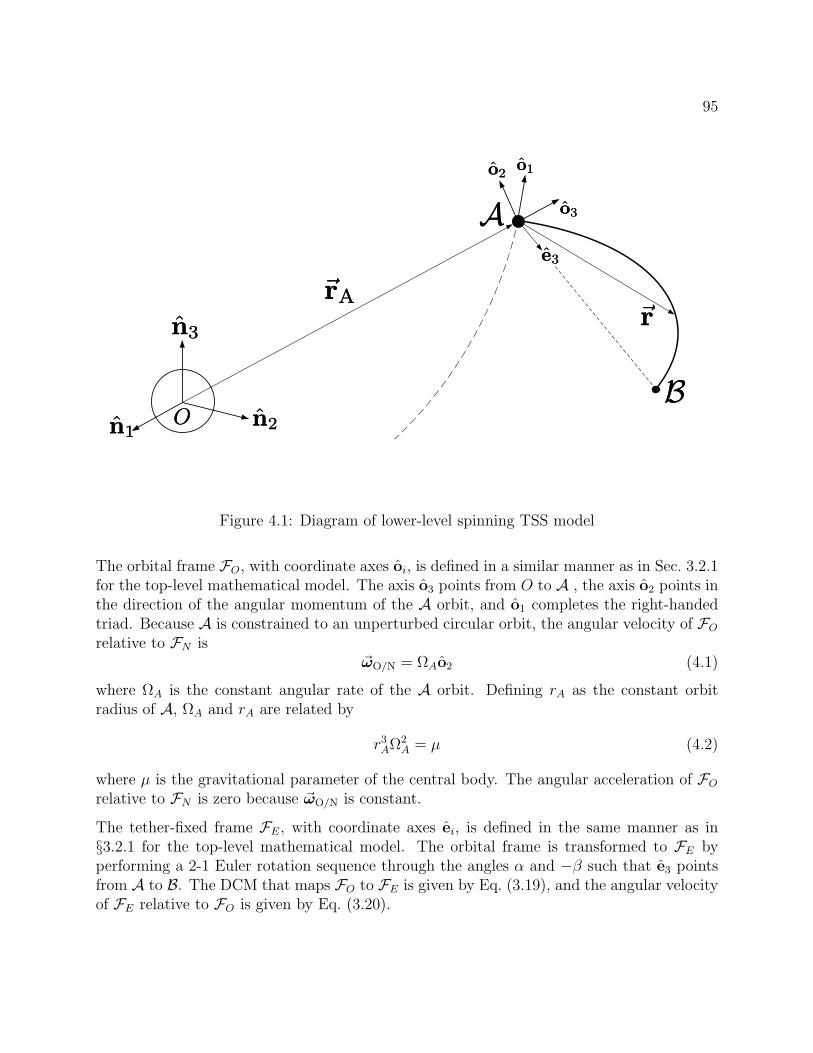
95

OO

AA

BB

e3e3

o1o1o2o2

o3o3

n1n1n2n2

n3n3

rArArr

Figure 4.1: Diagram of lower-level spinning TSS model

The orbital frame FO, with coordinate axes oi, is defined in a similar manner as in Sec. 3.2.1for the top-level mathematical model. The axis o3 points from O to A , the axis o2 points inthe direction of the angular momentum of the A orbit, and o1 completes the right-handedtriad. Because A is constrained to an unperturbed circular orbit, the angular velocity of FOrelative to FN is

~ωO/N = ΩAo2 (4.1)

where ΩA is the constant angular rate of the A orbit. Defining rA as the constant orbitradius of A, ΩA and rA are related by

r3AΩ2

A = µ (4.2)

where µ is the gravitational parameter of the central body. The angular acceleration of FOrelative to FN is zero because ~ωO/N is constant.

The tether-fixed frame FE, with coordinate axes ei, is defined in the same manner as in§3.2.1 for the top-level mathematical model. The orbital frame is transformed to FE byperforming a 2-1 Euler rotation sequence through the angles α and −β such that e3 pointsfrom A to B. The DCM that maps FO to FE is given by Eq. (3.19), and the angular velocityof FE relative to FO is given by Eq. (3.20).

96

4.2.2 Tether Geometry

As discussed in §3.2.2 for the top-level mathematical model, the position of a differentialtether element relative to A can be expressed as

~r(s, t) = se3 + ~u(s, t) (4.3)

where s is the unstretched arclength and ~u is the displacement of the tether away from itsunstretched state. Because we assume that the longitudinal displacement is negligible,

~u = U(s, t)e1 + V (s, t)e2 (4.4)

where U and V are transverse displacements, and Eq. (4.3) becomes

~r(s, t) = U(s, t)e1 + V (s, t)e2 + se3 (4.5)

Recall that the unit tangent vector of the tether is defined by Eq. (3.24). Using Eq. (4.5) inEq. (3.24), we have

τ (s, t) =∂U

∂s

∂s

∂se1 +

∂V

∂s

∂s

∂se2 +

∂s

∂se3 (4.6)

Because the transverse displacements are assumed to remain small, we make the approxi-mation

∂s

∂s≈ 1 (4.7)

such that the unit tangent vector is written as

τ (s, t) =∂U

∂se1 +

∂V

∂se2 + e3 (4.8)

Using Eq. (4.8), the tension in the tether is expressed as

~T(s, t) = T (s, t)τ (s, t)

= T

(∂U

∂se1 +

∂V

∂se2 + e3

)(4.9)

where T is the scalar tension in the tether. In this mathematical model we do not relate Tto the geometry of the tether, as done in the top-level mathematical model. Instead, we usean approximate expression for the tension that is derived by assuming that the transversedisplacements do not affect the tension, which is in accordance with the assumptions usedin the model. This derivation is presented later in this section.

97

4.2.3 Pendular Equations of Motion

Because we assume that the elastic vibrations of the tether do not affect the pendular motionof the tether, we derive the equations governing the pendular motion by assuming that thetether remains undeformed and aligned with e3. In this case, the entire system acts as arigid body, and the equations governing its motion are derived by treating it as a rigid body.

Applying Euler’s rotational equation to the undeformed system, we have

~IC · ~ωE/N + ~ωE/N ×~IC · ~ωE/N = ~MC (4.10)

where ~IC is the centroidal moment of inertia tensor of the system and ~MC is the totalexternal moment acting about the system mass center. Note that ~ωE/N is used as the bodyangular velocity in Eq. (4.10) because the undeformed system remains aligned with e3, soFE is a body-fixed frame for the undeformed system. Recall that one of the assumptionsmade in formulating the conceptual model is that A is much more massive than B and thetether, such that A remains on an unperturbed circular orbit. Another consequence of thisassumption is that the system mass center and A are essentially the same point, and we canapproximate Eq. (4.10) as

~IA · ~ωE/N + ~ωE/N ×~IA · ~ωE/N = ~MA (4.11)

where ~IA is the moment of inertia tensor of the system about A and ~MA is the total externalmoment acting on the system about A. Because all of the system mass in the undeformedsystem lies entirely along the e3 axis, ~IA is defined as

~IA = IA(1− e3e3) (4.12)

where IA is the scalar moment of inertia of the system about O and 1 is the identity tensor.Combining Eqs. (3.20) and (4.1), the angular velocity and acceleration of FE relative to FNare

~ωE/N = −βe1 + (α + ΩA) cos βe2 + (α + ΩA) sin βe3 (4.13)

~ωE/N = −βe1 + [α cos β − (α + ΩA)β sin β]e2 + [α sin β + (α + ΩA)β cos β]e3 (4.14)

The external moment acting on the system about A is due entirely to the gravity-gradientacting over the length of the system. Because the length of the system is small relative to theorbit radius of the system, we use a linear approximation for the gravity-gradient torque23

~MA = 3Ω2Ao3 ×~IA · o3 (4.15)

Combining Eqs. (4.11–4.15) and expressing the result relative to FE, we find that theequations governing the pendular motion of the tether are

α cos β − 2(α + ΩA)β sin β + 3Ω2A sinα cosα cos β = 0 (4.16)

β + [(α + ΩA)2 + 3Ω2A cos2 α] sin β cos β = 0 (4.17)

98

Note that these equations are identical to the equations governing the motion of a dumbbellsatellite constrained to a circular orbit.11 This makes sense, of course, because the unde-formed system is in fact a dumbbell satellite constrained to a circular orbit. This fact willbe utilized when analyzing Eqs. (4.16) and (4.17) later in this chapter.

4.2.4 Transverse Vibration Equations of Motion

The equations of motion for the transverse vibrations of the tether are derived in a similarmanner as the elastic vibration equations of motion for the top-level mathematical model.Following the steps outlined in §3.2.5 and omitting the electrodynamic force, the equationof motion of the tether is

~rT = − µ

r3T

~rT +1

ρ

∂~T

∂s(4.18)

where ~rT is the position of a differential tether element relative to O, rT is the magnitude of~rT, and ρ is the linear mass density of the undeformed tether. Noting that

~rT = ~rA +~r (4.19)

Eq. (4.18) is rewritten as

~r = − µ

r3T

~rT +1

ρ

∂~T

∂s− ~rA (4.20)

Using Eq. (4.9), the tension partial derivative term in Eq. (4.20) is

∂~T

∂s=

(T∂2U

∂s2+∂T

∂s

∂U

∂s

)e1 +

(T∂2V

∂s2+∂T

∂s

∂V

∂s

)e2 +

∂T

∂se3 (4.21)

Because A is constrained to a circular orbit,

~rA = −rAΩ2Ao3

= rAΩ2A(sinαe1 + cosα sin βe2 − cosα cos βe3)

(4.22)

As done in the derivation of the pendular equations of motion, because the length of thetether is small relative to the orbit radius of the system the gravitational acceleration termis approximated by linearizing about the position of A, such that

− µ

r3T

~rT = g1e1 + g2e2 + g3e3 (4.23)

where

g1 = Ω2A[rA sinα + U(3 sin2 α− 1) + 3V sinα cosα sin β − 3s sinα cosα cos β] (4.24)

99

g2 = Ω2A[ rA cosα sin β + 3U sinα cosα sin β + V (3 cos2 α sin2 β − 1)

− 3s cos2 α sin β cos β](4.25)

g3 = −Ω2A[ rA cosα cos β + 3U sinα cosα cos β + 3V cos2 α sin β cos β

+ s(1− 3 cos2 α cos2 β)](4.26)

Using the expression for ~r defined in Eq. (4.5), the left-hand side of Eq. (4.20) is written as

~r = r1e1 + r2e2 + r3e3 (4.27)

where

r1 =U − 2V (α + Ω2A) sin β − U(α + Ω2

A)2 − V [α sin β + 2(α + ΩA)β cos β]

+ s[α cos β − 2(α + ΩA)β sin β](4.28)

r2 =V + 2U(α + ΩA) sin β + Uα sin β − V [(α + ΩA)2 sin2 β + β2]

+ s[β + (α + ΩA)2 sin β cos β](4.29)

r3 =− 2U(α + ΩA) cos β − 2V β − Uα cos β − V [β − (α + ΩA)2 sin β cos β]

− s[(α + ΩA)2 cos2 β + β2](4.30)

Combining Eqs. (4.20–4.30) and taking the components in the e1 and e2 directions, theequations of motion for the transverse vibrations of the tether are

U − 2V (α + Ω2A) sin β − U [(α + Ω2

A)2 + Ω2A(3 sin2 α− 1)]

− V [α sin β + 2(α + ΩA)β cos β + 3Ω2A sinα cosα sin β]

+ s[α cos β − 2(α + ΩA)β sin β + 3Ω2A sinα cosα cos β]

=1

ρ

(T∂2U

∂s2+∂T

∂s

∂U

∂s

) (4.31)

V + 2U(α + ΩA) sin β + U(α sin β − 3Ω2A sinα cosα sin β)

− V [(α + ΩA)2 sin2 β + β2]

+ s[β + (α + ΩA)2 sin β cos β + 3Ω2A cos2 α sin β cos β]

=1

ρ

(T∂2V

∂s2+∂T

∂s

∂V

∂s

) (4.32)

Using the pendular equations of motion defined in Eqs. (4.16) and (4.17), the transversevibrations equations of motion reduce to

U − 2V (α + Ω2A) sin β − U [(α + Ω2

A)2 + Ω2A(3 sin2 α− 1)]− 2V (α + ΩA)β sec β

=1

ρ

(T∂2U

∂s2+∂T

∂s

∂U

∂s

)(4.33)

100

V + 2U(α + ΩA) sin β + 2U [(α + ΩA)β tan β − 3Ω2A sinα cosα] sin β

− V [(α + ΩA)2 sin2 β + β2 + Ω2A(3 cos2 α sin2 β − 1)]

=1

ρ

(T∂2V

∂s2+∂T

∂s

∂V

∂s

) (4.34)

To complete the equations of motion for the transverse vibrations we need an expression forthe tension in the tether. Taking the component of Eq. (4.20) in the e3 direction, we have

− 2U(α + ΩA) cos β − 2V β − U(α cos β − 3Ω2A sinα cosα cos β)

− V [β − (α + ΩA)2 sin β cos β − 3Ω2A cos2 α sin β cos β]

− s[(α + ΩA)2 cos2 β + β2 + Ω2A(3 cos2 α cos2 β − 1)]

=1

ρ

∂T

∂s

(4.35)

Now, recall that one of the assumptions made in the formulation of the conceptual model isthat the transverse vibrations do no affect the tension in the tether. Neglecting the transversevibration terms in Eq. (4.35), we find that the variation of the tension over the tether is

∂T

∂s= −ρs[(α + ΩA)2 cos2 β + β2 + Ω2

A(3 cos2 α cos2 β − 1)] (4.36)

Integrating Eq. (4.36) with respect to s, we obtain

T (s, t) = −1

2ρs2[(α + ΩA)2 cos2 β + β2 + Ω2

A(3 cos2 α cos2 β − 1)] + C (4.37)

where C is an integration constant. To determine C, we consider the motion of B, whichdefines the conditions of the tether at s = L. Applying Newton’s Second Law to B, theequation of motion of B is

mB~rB = −mBµ

r3B

~rB − ~T(L, t) (4.38)

where ~rB = ~rA +~r(L, t) is the position of B relative to O and mB is the mass of B. Using thelinear approximation for the gravitational acceleration term evaluated at s = L and takingthe component of Eq. (4.38) in the e3 direction, we find that the tension at B is

T (L, t) = mBL[(α + ΩA)2 cos2 β + β2 + Ω2A(3 cos2 α cos2 β − 1)] (4.39)

Setting s = L in Eq. (4.37), we must also have

T (L, t) = −1

2ρL2[(α + ΩA)2 cos2 β + β2 + Ω2

A(3 cos2 α cos2 β − 1)] + C (4.40)

Equating Eqs. (4.39) and (4.40), we find that the integration constant must be

C = cA[(α + ΩA)2 cos2 β + β2 + Ω2A(3 cos2 α cos2 β − 1)] (4.41)

101

where we have defined the quantity

cA = mBL+1

2ρL2 (4.42)

Note that cA is the first moment of inertia of the undeformed system about A. UsingEq. (4.41) in Eq. (4.37), the tension in the tether is expressed as

T (s, t) = [(α + ΩA)2 cos2 β + β2 + Ω2A(3 cos2 α cos2 β − 1)]

(cA −

1

2ρs2

)(4.43)

Using Eq. (4.43) in Eqs. (4.33) and (4.34), we obtain

U − 2V (α + Ω2A) sin β − U [(α + Ω2

A)2 + Ω2A(3 sin2 α− 1)]− 2V (α + ΩA)β sec β

= [(α + ΩA)2 cos2 β + β2 + Ω2A(3 cos2 α cos2 β − 1)]

[(cAρ− s2

2

)∂2U

∂s2− s∂U

∂s

](4.44)

V + 2U(α + ΩA) sin β + 2U [(α + ΩA)β tan β − 3Ω2A sinα cosα] sin β

− V [(α + ΩA)2 sin2 β + β2 + Ω2A(3 cos2 α sin2 β − 1)]

= [(α + ΩA)2 cos2 β + β2 + Ω2A(3 cos2 α cos2 β − 1)]

[(cAρ− s2

2

)∂2V

∂s2− s∂V

∂s

] (4.45)

Equations (4.44) and (4.45) are a set of coupled, second-order partial differential equationsthat govern the transverse vibrations of the tether. Because there can be no transversedisplacement at either end of the tether, the boundary conditions of Eqs. (4.44) and (4.45)are

U(0, t) = U(L, t) = 0 (4.46)

V (0, t) = V (L, t) = 0 (4.47)

4.2.5 Nondimensional Equations of Motion

The complete set of equations of motion governing the motion of the tether is given byEqs. (4.16), (4.17), and (4.44–4.47). These equations are cast in a nondimensional form byfirst defining the nondimensional time

τ = ΩAt (4.48)

and denoting derivatives with respect to τ as

( ). Note that τ is the angle through whichA moves in its circular orbit over a time t. Using the nondimensional time, the pendularequations of motion are written in nondimensional form as

α cos β − 2(

α + 1)

β sin β + 3 sinα cosα cos β = 0 (4.49)

β + [(

α + 1)2 + 3 cos2 α] sin β cos β = 0 (4.50)

102

To cast the transverse vibration equations of motion in nondimensional form we also definethe nondimensional spatial coordinate

x =s

L(4.51)

and denote derivatives with respect to x as ( )′. Let the nondimensional transverse displace-ments be defined as

u =U

L(4.52)

v =V

L(4.53)

and define the nondimensional parameter

γ =ρL2

cA(4.54)

Note that, using Eq. (4.42), we can also express γ as

γ =ρL

mB + 12ρL

(4.55)

From Eq. (4.55), we can see that γ ∈ [0, 2], with γ = 0 corresponding to a massless tetherand γ = 2 corresponding to mB = 0. Using Eqs. (4.48) and (4.51–4.55), the transversevibration equations of motion and boundary conditions are written in nondimensional formas

u− 2

v(α + 1) sin β − u[(

α + 1)2 + 3 sin2 α− 1]− 2v(

α + 1)

β sec β

= [(α + 1)2 cos2 β +

β2 + 3 cos2 α cos2 β − 1]

[(2− γx2

2γ

)u′′ − xu′

](4.56)

v + 2

u(α + 1) sin β + 2u[(

α + 1)

β tan β − 3 sinα cosα] sin β

− v[(α + 1)2 sin2 β +

β2 + 3 cos2 α sin2 β − 1]

= [(α + 1)2 cos2 β +

β2 + 3 cos2 α cos2 β − 1]

[(2− γx2

2γ

)v′′ − xv′

] (4.57)

u(0, τ) = u(1, τ) = 0 (4.58)

v(0, τ) = v(1, τ) = 0 (4.59)

Equations (4.49), (4.50), and (4.56–4.57) define the complete set of nondimensional equationsof motion for the system. In the next two sections, several aspects of the computationalmodel for the lower-level system model considered in this chapter are developed using theseequations.

103

4.3 Computational Model: Pendular Motion of the

Tether

In this section we develop several aspects of the lower-level computational model for thespinning TSS. Specifically, in this section we focus on the pendular motion of the tether. Re-call that the equations governing the pendular motion of the tether, Eqs. (4.49) and (4.50),are the same as the attitude equations of motion for a dumbbell satellite constrained to acircular orbit acted upon only by gravity-gradient torque. A dumbbell satellite is a specialtype of rigid satellite model, so the analysis of the tether pendular motion is the same asthe analysis of a spinning rigid body on a circular orbit acted upon only by gravity-gradienttorque. Kane and Shippy27 studied such a system by assuming that the deviations awayfrom the nominal spinning trajectory were small and linearizing the equations of motionabout the nominal spin. For small out-of-plane motion, the in-plane motion is not affectedby the out-of-plane motion, and an exact solution for the in-plane motion was determined.This solution was used in the linearized equations for the out-of-plane motion, resulting ina system of homogeneous linear equations with periodic, time-varying coefficients. Floquettheory was applied to determine the stability properties of the out-of-plane motion for vari-ous combinations of satellite inertia parameters and average in-plane spin rate. Because oflimitations in computing power at the time, only a few specific cases were considered; how-ever, it was demonstrated that the out-of-plane motion is unstable for certain combinationsof inertia parameters and average in-plane spin rate. Meirovitch and Wallace40 used purelyanalytical methods to extend the analysis of Kane and Shippy by assuming that the satelliteis nearly symmetric about the spin axis. This assumption cannot be applied to a spinningTSS, so the extended results of Meirvitch and Wallace do not apply to the present study ofspinning TSS pendular motion. Kane26 applied the same analysis methods used by Kaneand Shippy to a nominally Earth-pointing satellite and showed that the out-of-plane motionis unstable for certain combinations of satellite inertia parameters and in-plane librationamplitude. Once again, limitations in computing power limited the analysis to a few specificcases. Breakwell and Pringle9 later showed that the instability in the out-of-plane motiondiscovered by Kane is due to a nonlinear internal resonance within the system equations ofmotion.

The results outlined in the previous paragraph clearly indicate that the system model usedin this chapter will predict unstable out-of-plane pendular motion for certain system config-urations. The description of these instabilities is not complete, however, because previousresearch has only considered a handful of specific cases, or made assumptions about thesystem geometry that do not apply to a spinning TSS. Modern computing power allows usto make a complete description of the out-of-plane motion and any associated instabilities.In addition, the analysis of a spinning TSS requires the variation of only a single parameterbecause the inertia ratios are set values for any TSS. Because of this fact, the analysis pre-sented in this section can be viewed as an application of the results of Refs. [27] and [26] toa specific type of spinning satellite (a TSS); however, the analysis presented in this section

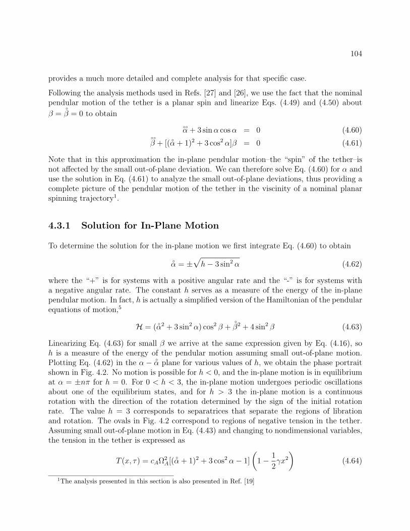
104

provides a much more detailed and complete analysis for that specific case.

Following the analysis methods used in Refs. [27] and [26], we use the fact that the nominalpendular motion of the tether is a planar spin and linearize Eqs. (4.49) and (4.50) about

β =β = 0 to obtain

α + 3 sinα cosα = 0 (4.60)

β + [(

α + 1)2 + 3 cos2 α]β = 0 (4.61)

Note that in this approximation the in-plane pendular motion–the “spin” of the tether–isnot affected by the small out-of-plane deviation. We can therefore solve Eq. (4.60) for α anduse the solution in Eq. (4.61) to analyze the small out-of-plane deviations, thus providing acomplete picture of the pendular motion of the tether in the viscinity of a nominal planarspinning trajectory1.

4.3.1 Solution for In-Plane Motion

To determine the solution for the in-plane motion we first integrate Eq. (4.60) to obtain

α = ±

√h− 3 sin2 α (4.62)

where the “+” is for systems with a positive angular rate and the “-” is for systems witha negative angular rate. The constant h serves as a measure of the energy of the in-planependular motion. In fact, h is actually a simplified version of the Hamiltonian of the pendularequations of motion,5

H = (α2 + 3 sin2 α) cos2 β +

β2 + 4 sin2 β (4.63)

Linearizing Eq. (4.63) for small β we arrive at the same expression given by Eq. (4.16), soh is a measure of the energy of the pendular motion assuming small out-of-plane motion.Plotting Eq. (4.62) in the α −

α plane for various values of h, we obtain the phase portraitshown in Fig. 4.2. No motion is possible for h < 0, and the in-plane motion is in equilibriumat α = ±nπ for h = 0. For 0 < h < 3, the in-plane motion undergoes periodic oscillationsabout one of the equilibrium states, and for h > 3 the in-plane motion is a continuousrotation with the direction of the rotation determined by the sign of the initial rotationrate. The value h = 3 corresponds to separatrices that separate the regions of librationand rotation. The ovals in Fig. 4.2 correspond to regions of negative tension in the tether.Assuming small out-of-plane motion in Eq. (4.43) and changing to nondimensional variables,the tension in the tether is expressed as

T (x, τ) = cAΩ2A[(

α + 1)2 + 3 cos2 α− 1]

(1− 1

2γx2

)(4.64)

1The analysis presented in this section is also presented in Ref. [19]

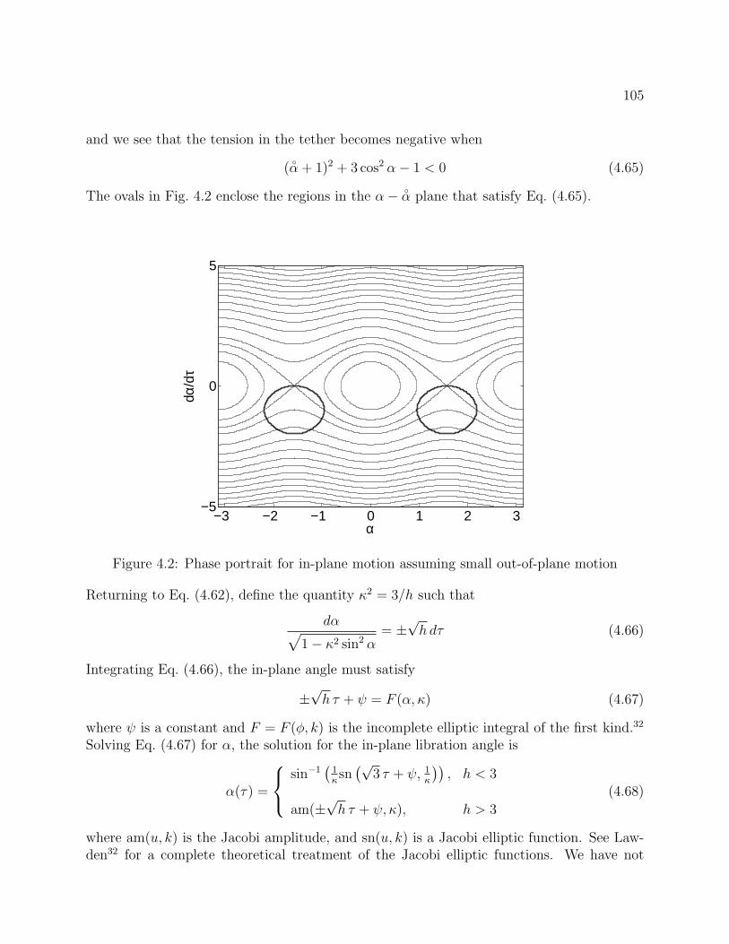
105

and we see that the tension in the tether becomes negative when

(α + 1)2 + 3 cos2 α− 1 < 0 (4.65)

The ovals in Fig. 4.2 enclose the regions in the α− α plane that satisfy Eq. (4.65).

α

dα/d

τ

−3 −2 −1 0 1 2 3−5

0

5

Figure 4.2: Phase portrait for in-plane motion assuming small out-of-plane motion

Returning to Eq. (4.62), define the quantity κ2 = 3/h such that

dα√1− κ2 sin2 α

= ±√h dτ (4.66)

Integrating Eq. (4.66), the in-plane angle must satisfy

±√h τ + ψ = F (α, κ) (4.67)

where ψ is a constant and F = F (φ, k) is the incomplete elliptic integral of the first kind.32

Solving Eq. (4.67) for α, the solution for the in-plane libration angle is

α(τ) =

sin−1

(1κsn(√

3 τ + ψ, 1κ

)), h < 3

am(±√h τ + ψ, κ), h > 3

(4.68)

where am(u, k) is the Jacobi amplitude, and sn(u, k) is a Jacobi elliptic function. See Law-den32 for a complete theoretical treatment of the Jacobi elliptic functions. We have not

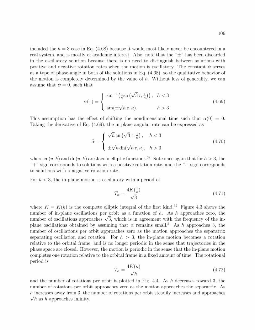
106

included the h = 3 case in Eq. (4.68) because it would most likely never be encountered in areal system, and is mostly of academic interest. Also, note that the “±” has been discardedin the oscillatory solution because there is no need to distinguish between solutions withpositive and negative rotation rates when the motion is oscillatory. The constant ψ servesas a type of phase-angle in both of the solutions in Eq. (4.68), so the qualitative behavior ofthe motion is completely determined by the value of h. Without loss of generality, we canassume that ψ = 0, such that

α(τ) =

sin−1

(1κsn(√

3 τ, 1κ

)), h < 3

am(±√h τ, κ), h > 3

(4.69)

This assumption has the effect of shifting the nondimensional time such that α(0) = 0.Taking the derivative of Eq. (4.69), the in-plane angular rate can be expressed as

α =

√h cn

(√3 τ, 1

κ

), h < 3

±√h dn(

√h τ, κ), h > 3

(4.70)

where cn(u, k) and dn(u, k) are Jacobi elliptic functions.32 Note once again that for h > 3, the“+” sign corresponds to solutions with a positive rotation rate, and the “-” sign correspondsto solutions with a negative rotation rate.

For h < 3, the in-plane motion is oscillatory with a period of

Tα =4K( 1

κ)

√3

(4.71)

where K = K(k) is the complete elliptic integral of the first kind.32 Figure 4.3 shows thenumber of in-plane oscillations per orbit as a function of h. As h approaches zero, thenumber of oscillations approaches

√3, which is in agreement with the frequency of the in-

plane oscillations obtained by assuming that α remains small.5 As h approaches 3, thenumber of oscillations per orbit approaches zero as the motion approaches the separatrixseparating oscillation and rotation. For h > 3, the in-plane motion becomes a rotationrelative to the orbital frame, and is no longer periodic in the sense that trajectories in thephase space are closed. However, the motion is periodic in the sense that the in-plane motioncompletes one rotation relative to the orbital frame in a fixed amount of time. The rotationalperiod is

Tα =4K(κ)√

h(4.72)

and the number of rotations per orbit is plotted in Fig. 4.4. As h decreases toward 3, thenumber of rotations per orbit approaches zero as the motion approaches the separatrix. Ash increases away from 3, the number of rotations per orbit steadily increases and approaches√h as h approaches infinity.

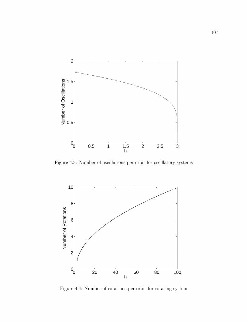
107

0 0.5 1 1.5 2 2.5 30

0.5

1

1.5

2

h

Num

ber

of O

scill

atio

ns

Figure 4.3: Number of oscillations per orbit for oscillatory systems

0 20 40 60 80 1000

2

4

6

8

10

h

Num

ber

of R

otat

ions

Figure 4.4: Number of rotations per orbit for rotating system

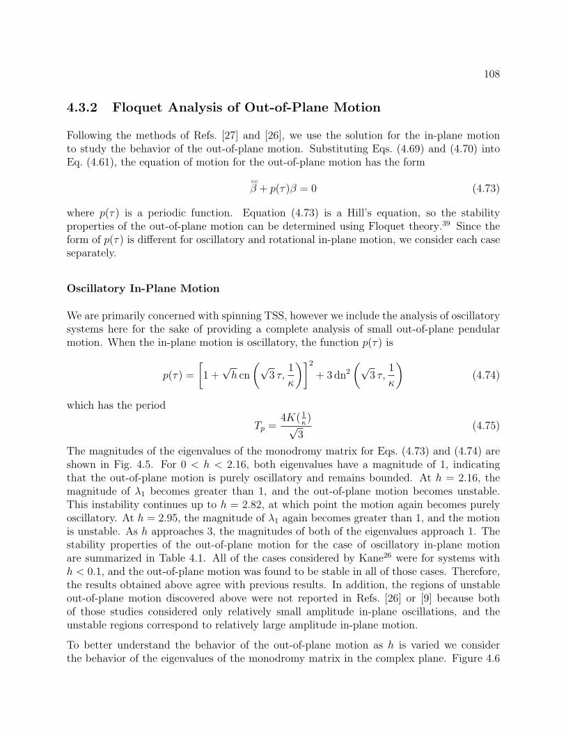
108

4.3.2 Floquet Analysis of Out-of-Plane Motion

Following the methods of Refs. [27] and [26], we use the solution for the in-plane motionto study the behavior of the out-of-plane motion. Substituting Eqs. (4.69) and (4.70) intoEq. (4.61), the equation of motion for the out-of-plane motion has the form

β + p(τ)β = 0 (4.73)

where p(τ) is a periodic function. Equation (4.73) is a Hill’s equation, so the stabilityproperties of the out-of-plane motion can be determined using Floquet theory.39 Since theform of p(τ) is different for oscillatory and rotational in-plane motion, we consider each caseseparately.

Oscillatory In-Plane Motion

We are primarily concerned with spinning TSS, however we include the analysis of oscillatorysystems here for the sake of providing a complete analysis of small out-of-plane pendularmotion. When the in-plane motion is oscillatory, the function p(τ) is

p(τ) =

[1 +√h cn

(√3 τ,

1

κ

)]2

+ 3 dn2

(√3 τ,

1

κ

)(4.74)

which has the period

Tp =4K( 1

κ)

√3

(4.75)

The magnitudes of the eigenvalues of the monodromy matrix for Eqs. (4.73) and (4.74) areshown in Fig. 4.5. For 0 < h < 2.16, both eigenvalues have a magnitude of 1, indicatingthat the out-of-plane motion is purely oscillatory and remains bounded. At h = 2.16, themagnitude of λ1 becomes greater than 1, and the out-of-plane motion becomes unstable.This instability continues up to h = 2.82, at which point the motion again becomes purelyoscillatory. At h = 2.95, the magnitude of λ1 again becomes greater than 1, and the motionis unstable. As h approaches 3, the magnitudes of both of the eigenvalues approach 1. Thestability properties of the out-of-plane motion for the case of oscillatory in-plane motionare summarized in Table 4.1. All of the cases considered by Kane26 were for systems withh < 0.1, and the out-of-plane motion was found to be stable in all of those cases. Therefore,the results obtained above agree with previous results. In addition, the regions of unstableout-of-plane motion discovered above were not reported in Refs. [26] or [9] because bothof those studies considered only relatively small amplitude in-plane oscillations, and theunstable regions correspond to relatively large amplitude in-plane motion.

To better understand the behavior of the out-of-plane motion as h is varied we considerthe behavior of the eigenvalues of the monodromy matrix in the complex plane. Figure 4.6

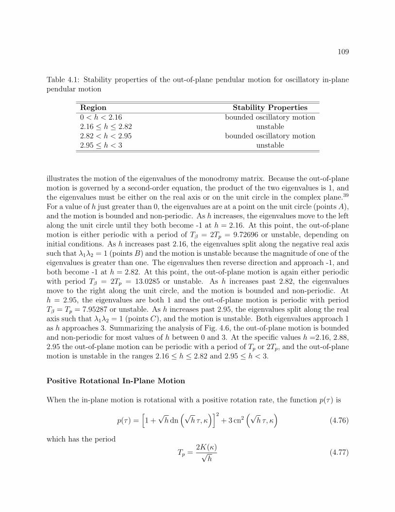
109

Table 4.1: Stability properties of the out-of-plane pendular motion for oscillatory in-planependular motion

Region Stability Properties0 < h < 2.16 bounded oscillatory motion2.16 ≤ h ≤ 2.82 unstable2.82 < h < 2.95 bounded oscillatory motion2.95 ≤ h < 3 unstable

illustrates the motion of the eigenvalues of the monodromy matrix. Because the out-of-planemotion is governed by a second-order equation, the product of the two eigenvalues is 1, andthe eigenvalues must be either on the real axis or on the unit circle in the complex plane.39

For a value of h just greater than 0, the eigenvalues are at a point on the unit circle (points A),and the motion is bounded and non-periodic. As h increases, the eigenvalues move to the leftalong the unit circle until they both become -1 at h = 2.16. At this point, the out-of-planemotion is either periodic with a period of Tβ = 2Tp = 9.72696 or unstable, depending oninitial conditions. As h increases past 2.16, the eigenvalues split along the negative real axissuch that λ1λ2 = 1 (points B) and the motion is unstable because the magnitude of one of theeigenvalues is greater than one. The eigenvalues then reverse direction and approach -1, andboth become -1 at h = 2.82. At this point, the out-of-plane motion is again either periodicwith period Tβ = 2Tp = 13.0285 or unstable. As h increases past 2.82, the eigenvaluesmove to the right along the unit circle, and the motion is bounded and non-periodic. Ath = 2.95, the eigenvalues are both 1 and the out-of-plane motion is periodic with periodTβ = Tp = 7.95287 or unstable. As h increases past 2.95, the eigenvalues split along the realaxis such that λ1λ2 = 1 (points C), and the motion is unstable. Both eigenvalues approach 1as h approaches 3. Summarizing the analysis of Fig. 4.6, the out-of-plane motion is boundedand non-periodic for most values of h between 0 and 3. At the specific values h =2.16, 2.88,2.95 the out-of-plane motion can be periodic with a period of Tp or 2Tp, and the out-of-planemotion is unstable in the ranges 2.16 ≤ h ≤ 2.82 and 2.95 ≤ h < 3.

Positive Rotational In-Plane Motion

When the in-plane motion is rotational with a positive rotation rate, the function p(τ) is

p(τ) =[1 +√h dn

(√h τ, κ

)]2

+ 3 cn2(√

h τ, κ)

(4.76)

which has the period

Tp =2K(κ)√

h(4.77)

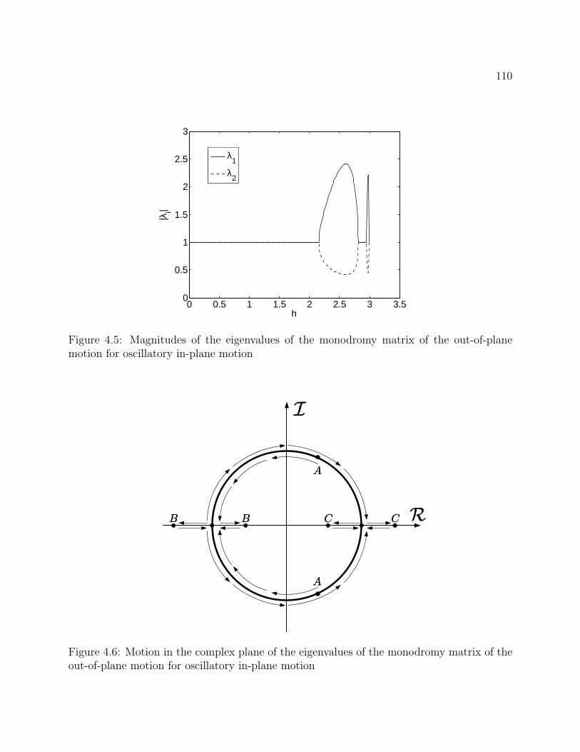
110

0 0.5 1 1.5 2 2.5 3 3.50

0.5

1

1.5

2

2.5

3

h

|λi|

λ1

λ2

Figure 4.5: Magnitudes of the eigenvalues of the monodromy matrix of the out-of-planemotion for oscillatory in-plane motion

RR

II

AA

AA

BBBB CC CC

Figure 4.6: Motion in the complex plane of the eigenvalues of the monodromy matrix of theout-of-plane motion for oscillatory in-plane motion

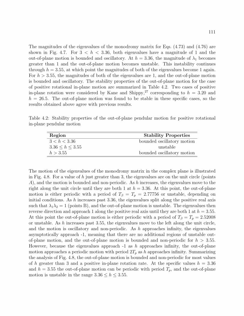
111

The magnitudes of the eigenvalues of the monodromy matrix for Eqs. (4.73) and (4.76) areshown in Fig. 4.7. For 3 < h < 3.36, both eigenvalues have a magnitude of 1 and theout-of-plane motion is bounded and oscillatory. At h = 3.36, the magnitude of λ1 becomesgreater than 1 and the out-of-plane motion becomes unstable. This instability continuesthrough h = 3.55, at which point the magnitudes of both of the eigenvalues become 1 again.For h > 3.55, the magnitudes of both of the eigenvalues are 1, and the out-of-plane motionis bounded and oscillatory. The stability properties of the out-of-plane motion for the caseof positive rotational in-plane motion are summarized in Table 4.2. Two cases of positivein-plane rotation were considered by Kane and Shippy,27 corresponding to h = 3.20 andh = 26.5. The out-of-plane motion was found to be stable in these specific cases, so theresults obtained above agree with previous results.

Table 4.2: Stability properties of the out-of-plane pendular motion for positive rotationalin-plane pendular motion

Region Stability Properties3 < h < 3.36 bounded oscillatory motion3.36 ≤ h ≤ 3.55 unstableh > 3.55 bounded oscillatory motion

The motion of the eigenvalues of the monodromy matrix in the complex plane is illustratedin Fig. 4.8. For a value of h just greater than 3, the eigenvalues are on the unit circle (pointsA), and the motion is bounded and non-periodic. As h increases, the eigenvalues move to theright along the unit circle until they are both 1 at h = 3.36. At this point, the out-of-planemotion is either periodic with a period of Tβ = Tp = 2.77756 or unstable, depending oninitial conditions. As h increases past 3.36, the eigenvalues split along the positive real axissuch that λ1λ2 = 1 (points B), and the out-of-plane motion is unstable. The eigenvalues thenreverse direction and approach 1 along the positive real axis until they are both 1 at h = 3.55.At this point the out-of-plane motion is either periodic with a period of Tβ = Tp = 2.52008or unstable. As h increases past 3.55, the eigenvalues move to the left along the unit circle,and the motion is oscillatory and non-periodic. As h approaches infinity, the eigenvaluesasymptotically approach -1, meaning that there are no additional regions of unstable out-of-plane motion, and the out-of-plane motion is bounded and non-periodic for h > 3.55.However, because the eigenvalues approach -1 as h approaches infinity, the out-of-planemotion approaches a periodic motion with period 2Tp as h approaches infinity. Summarizingthe analysis of Fig. 4.8, the out-of-plane motion is bounded and non-periodic for most valuesof h greater than 3 and a positive in-plane rotation rate. At the specific values h = 3.36and h = 3.55 the out-of-plane motion can be periodic with period Tp, and the out-of-planemotion is unstable in the range 3.36 ≤ h ≤ 3.55.

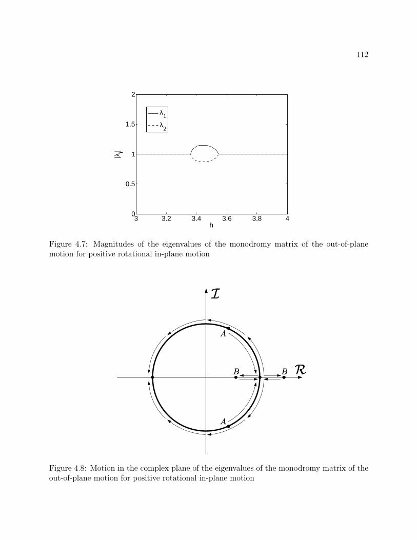
112

3 3.2 3.4 3.6 3.8 40

0.5

1

1.5

2

h

|λi|

λ1

λ2

Figure 4.7: Magnitudes of the eigenvalues of the monodromy matrix of the out-of-planemotion for positive rotational in-plane motion

RR

II

AA

AA

BBBB

Figure 4.8: Motion in the complex plane of the eigenvalues of the monodromy matrix of theout-of-plane motion for positive rotational in-plane motion

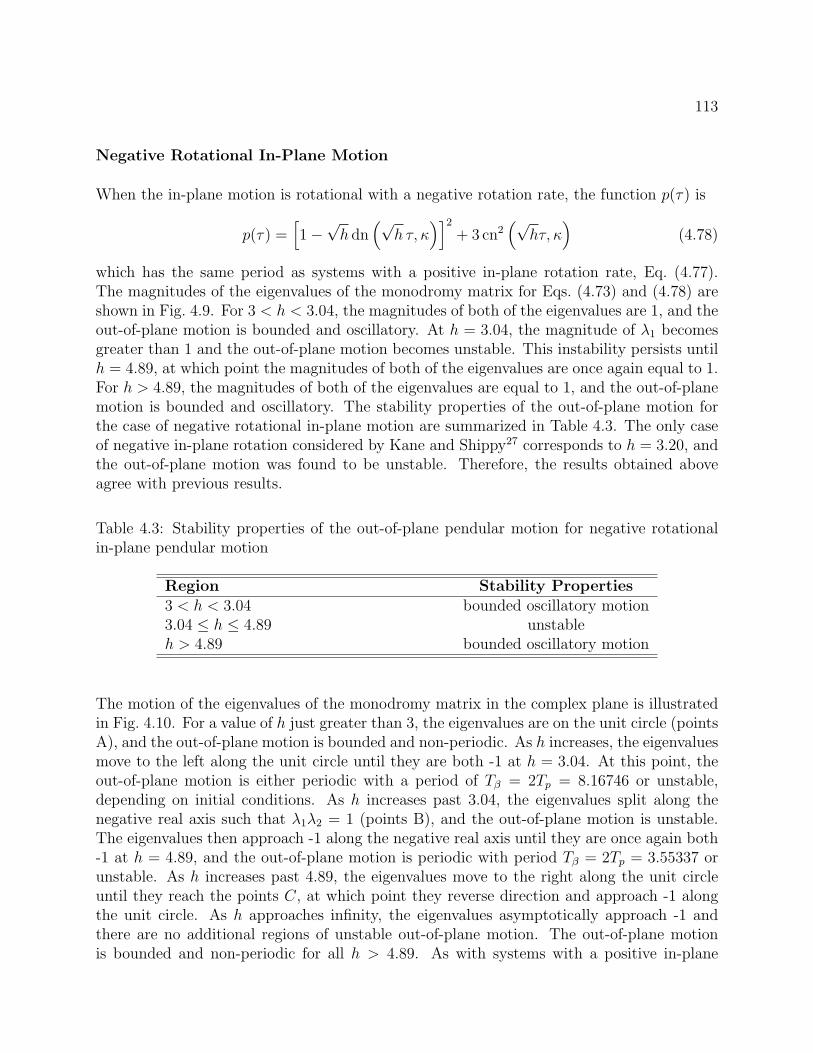
113

Negative Rotational In-Plane Motion

When the in-plane motion is rotational with a negative rotation rate, the function p(τ) is

p(τ) =[1−√h dn

(√h τ, κ

)]2

+ 3 cn2(√

hτ, κ)

(4.78)

which has the same period as systems with a positive in-plane rotation rate, Eq. (4.77).The magnitudes of the eigenvalues of the monodromy matrix for Eqs. (4.73) and (4.78) areshown in Fig. 4.9. For 3 < h < 3.04, the magnitudes of both of the eigenvalues are 1, and theout-of-plane motion is bounded and oscillatory. At h = 3.04, the magnitude of λ1 becomesgreater than 1 and the out-of-plane motion becomes unstable. This instability persists untilh = 4.89, at which point the magnitudes of both of the eigenvalues are once again equal to 1.For h > 4.89, the magnitudes of both of the eigenvalues are equal to 1, and the out-of-planemotion is bounded and oscillatory. The stability properties of the out-of-plane motion forthe case of negative rotational in-plane motion are summarized in Table 4.3. The only caseof negative in-plane rotation considered by Kane and Shippy27 corresponds to h = 3.20, andthe out-of-plane motion was found to be unstable. Therefore, the results obtained aboveagree with previous results.

Table 4.3: Stability properties of the out-of-plane pendular motion for negative rotationalin-plane pendular motion

Region Stability Properties3 < h < 3.04 bounded oscillatory motion3.04 ≤ h ≤ 4.89 unstableh > 4.89 bounded oscillatory motion

The motion of the eigenvalues of the monodromy matrix in the complex plane is illustratedin Fig. 4.10. For a value of h just greater than 3, the eigenvalues are on the unit circle (pointsA), and the out-of-plane motion is bounded and non-periodic. As h increases, the eigenvaluesmove to the left along the unit circle until they are both -1 at h = 3.04. At this point, theout-of-plane motion is either periodic with a period of Tβ = 2Tp = 8.16746 or unstable,depending on initial conditions. As h increases past 3.04, the eigenvalues split along thenegative real axis such that λ1λ2 = 1 (points B), and the out-of-plane motion is unstable.The eigenvalues then approach -1 along the negative real axis until they are once again both-1 at h = 4.89, and the out-of-plane motion is periodic with period Tβ = 2Tp = 3.55337 orunstable. As h increases past 4.89, the eigenvalues move to the right along the unit circleuntil they reach the points C, at which point they reverse direction and approach -1 alongthe unit circle. As h approaches infinity, the eigenvalues asymptotically approach -1 andthere are no additional regions of unstable out-of-plane motion. The out-of-plane motionis bounded and non-periodic for all h > 4.89. As with systems with a positive in-plane

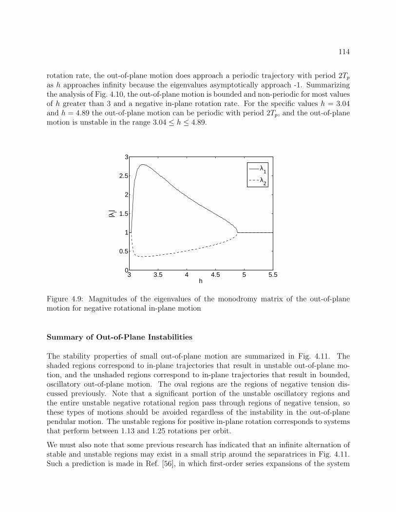
114

rotation rate, the out-of-plane motion does approach a periodic trajectory with period 2Tpas h approaches infinity because the eigenvalues asymptotically approach -1. Summarizingthe analysis of Fig. 4.10, the out-of-plane motion is bounded and non-periodic for most valuesof h greater than 3 and a negative in-plane rotation rate. For the specific values h = 3.04and h = 4.89 the out-of-plane motion can be periodic with period 2Tp, and the out-of-planemotion is unstable in the range 3.04 ≤ h ≤ 4.89.

3 3.5 4 4.5 5 5.50

0.5

1

1.5

2

2.5

3

h

|λi|

λ1

λ2

Figure 4.9: Magnitudes of the eigenvalues of the monodromy matrix of the out-of-planemotion for negative rotational in-plane motion

Summary of Out-of-Plane Instabilities

The stability properties of small out-of-plane motion are summarized in Fig. 4.11. Theshaded regions correspond to in-plane trajectories that result in unstable out-of-plane mo-tion, and the unshaded regions correspond to in-plane trajectories that result in bounded,oscillatory out-of-plane motion. The oval regions are the regions of negative tension dis-cussed previously. Note that a significant portion of the unstable oscillatory regions andthe entire unstable negative rotational region pass through regions of negative tension, sothese types of motions should be avoided regardless of the instability in the out-of-planependular motion. The unstable regions for positive in-plane rotation corresponds to systemsthat perform between 1.13 and 1.25 rotations per orbit.

We must also note that some previous research has indicated that an infinite alternation ofstable and unstable regions may exist in a small strip around the separatrices in Fig. 4.11.Such a prediction is made in Ref. [56], in which first-order series expansions of the system

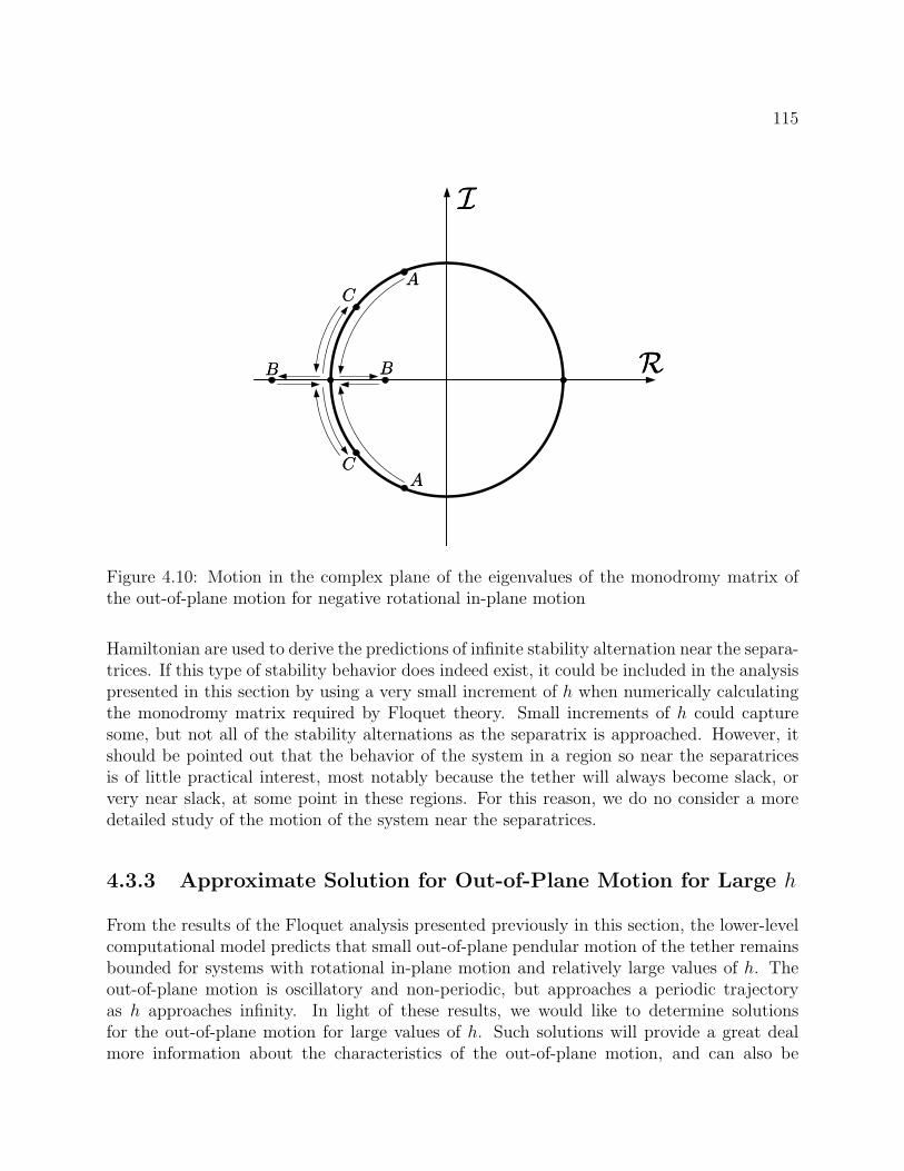
115

RR

II

AA

AA

BB BB

CC

CC

Figure 4.10: Motion in the complex plane of the eigenvalues of the monodromy matrix ofthe out-of-plane motion for negative rotational in-plane motion

Hamiltonian are used to derive the predictions of infinite stability alternation near the separa-trices. If this type of stability behavior does indeed exist, it could be included in the analysispresented in this section by using a very small increment of h when numerically calculatingthe monodromy matrix required by Floquet theory. Small increments of h could capturesome, but not all of the stability alternations as the separatrix is approached. However, itshould be pointed out that the behavior of the system in a region so near the separatricesis of little practical interest, most notably because the tether will always become slack, orvery near slack, at some point in these regions. For this reason, we do no consider a moredetailed study of the motion of the system near the separatrices.

4.3.3 Approximate Solution for Out-of-Plane Motion for Large h

From the results of the Floquet analysis presented previously in this section, the lower-levelcomputational model predicts that small out-of-plane pendular motion of the tether remainsbounded for systems with rotational in-plane motion and relatively large values of h. Theout-of-plane motion is oscillatory and non-periodic, but approaches a periodic trajectoryas h approaches infinity. In light of these results, we would like to determine solutionsfor the out-of-plane motion for large values of h. Such solutions will provide a great dealmore information about the characteristics of the out-of-plane motion, and can also be

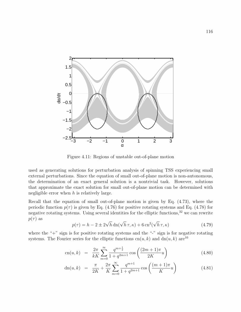
116

−3 −2 −1 0 1 2 3−2.5

−2

−1.5

−1

−0.5

0

0.5

1

1.5

2

α

dα/d

τ

Figure 4.11: Regions of unstable out-of-plane motion

used as generating solutions for perturbation analysis of spinning TSS experiencing smallexternal perturbations. Since the equation of small out-of-plane motion is non-autonomous,the determination of an exact general solution is a nontrivial task. However, solutionsthat approximate the exact solution for small out-of-plane motion can be determined withnegligible error when h is relatively large.

Recall that the equation of small out-of-plane motion is given by Eq. (4.73), where theperiodic function p(τ) is given by Eq. (4.76) for positive rotating systems and Eq. (4.78) fornegative rotating systems. Using several identities for the elliptic functions,32 we can rewritep(τ) as

p(τ) = h− 2± 2√h dn(

√h τ, κ) + 6 cn2(

√h τ, κ) (4.79)

where the “+” sign is for positive rotating systems and the “-” sign is for negative rotatingsystems. The Fourier series for the elliptic functions cn(u, k) and dn(u, k) are10

cn(u, k) =2π

kK

∞∑m=0

qm+ 12

1 + q2m+1cos

((2m+ 1)π

2Ku

)(4.80)

dn(u, k) =π

2K+

2π

K

∞∑m=0

qm+1

1 + q2m+1cos

((m+ 1)π

Ku

)(4.81)

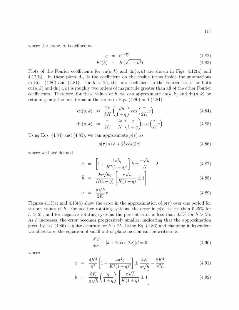
117

where the nome, q, is defined as

q = e−πK′K (4.82)

K ′(k) = K(√

1− k2) (4.83)

Plots of the Fourier coefficients for cn(u, k) and dn(u, k) are shown in Figs. 4.12(a) and4.12(b). In these plots Am is the coefficient on the cosine terms inside the summationsin Eqs. (4.80) and (4.81). For h > 25, the first coefficient in the Fourier series for bothcn(u, k) and dn(u, k) is roughly two orders of magnitude greater than all of the other Fouriercoefficients. Therefore, for these values of h, we can approximate cn(u, k) and dn(u, k) byretaining only the first terms in the series in Eqs. (4.80) and (4.81),

cn(u, k) ≈ 2π

kK

( √q

1 + q

)cos( π

2Ku)

(4.84)

dn(u, k) ≈ π

2K+

2π

K

(q

1 + q

)cos( πKu)

(4.85)

Using Eqs. (4.84) and (4.85), we can approximate p(τ) as

p(τ) ≈ a+ 2b cos(2ν) (4.86)


a =

[1 +

4π2q

K2(1 + q)2

]h± π

√h

K− 2 (4.87)

b =2π√hq

K(1 + q)

[π√h

K(1 + q)± 1

](4.88)

ν =π√h

2Kτ (4.89)

Figures 4.13(a) and 4.13(b) show the error in the approximation of p(τ) over one period forvarious values of h. For positive rotating systems, the error in p(τ) is less than 0.25% forh > 25, and for negative rotating systems the percent error is less than 0.5% for h > 25.As h increases, the error becomes progressively smaller, indicating that the approximationgiven by Eq. (4.86) is quite accurate for h > 25. Using Eq. (4.86) and changing independentvariables to ν, the equation of small out-of-plane motion can be written as

d2β

dν2+ [a+ 2b cos(2ν)]β = 0 (4.90)

where

a =4K2

π2

[1 +

4π2q

K2(1 + q)2

]± 4K

π√h− 8K2

π2h(4.91)

b =8K

π√h

(q

1 + q

)[π√h

K(1 + q)± 1

](4.92)

118

Equation (4.90) is recognized as Mathieu’s equation,37 for which we can use Floquet’s theo-rem to determine an approximate analytical solution.

Floquet’s theorem states that a solution to Eq. (4.90) can be written as39

β(ν) = eρνφ(ν) (4.93)

where ρ is the characteristic exponent and φ(ν) is a periodic function of ν with period π.Note that, in general, both ρ and φ are complex. Because φ(ν) is periodic, we can expandit in a Fourier series such that

β(ν) = eρν∞∑

n=−∞

cne2inν (4.94)

where cn are the coefficients of the series. Rewriting p(ν) as

p(ν) = a+ b(e2iν + e−2iν) (4.95)

and using Eq. (4.94), we can rewrite Eq. (4.90) as

∞∑n=−∞

(ρ+ 2in)2cne(ρ+2in)ν + [a+ b(e2iν + e−2iν)]

∞∑n=−∞

cne(ρ+2in)ν = 0 (4.96)

Collecting powers of e2inν , we obtain the following infinite set of linear algebraic equationsfor the Fourier coefficients,

bcn−1 + [a+ (ρ+ 2in)2]cn + bcn+1 = 0, n = −∞, ...,∞ (4.97)

The system of equations given by Eq. (4.97) can be written in matrix form as

Ac = 0 (4.98)

where A is an infinite tri-diagonal matrix, c is a column matrix containing all of the Fouriercoefficients, and 0 is the infinite zero column matrix. For Eq. (4.98) to have a non-trivialsolution, the determinant of A, ∆, must be zero. It can be shown that37,39

∆(iρ) = ∆(0)− sin2

(1

2πiρ

)csc2

(1

2π√a

)(4.99)

so the characteristic exponent must satisfy the transcendental equation

sin2

(1

2πiρ

)= ∆(0) sin2

(1

2π√a

)(4.100)

If b2 1, then we can approximate ∆(0) as37

∆(0) ≈ 1−πb2cot

(12π√a)

4√a(a− 1)

(4.101)

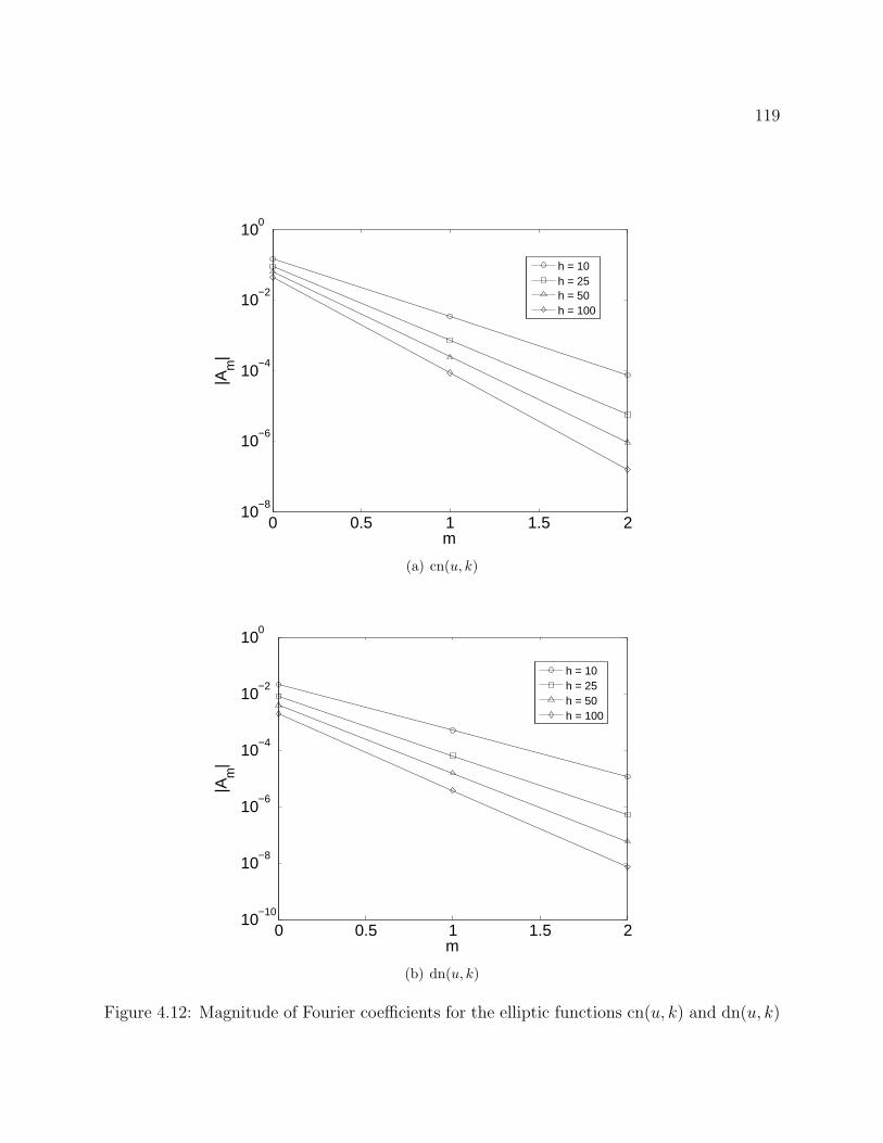
119

0 0.5 1 1.5 210

−8

10−6

10−4

10−2

100

m

|Am

|

h = 10h = 25h = 50h = 100

(a) cn(u, k)

0 0.5 1 1.5 210

−10

10−8

10−6

10−4

10−2

100

m

|Am

|

h = 10h = 25h = 50h = 100

(b) dn(u, k)

Figure 4.12: Magnitude of Fourier coefficients for the elliptic functions cn(u, k) and dn(u, k)

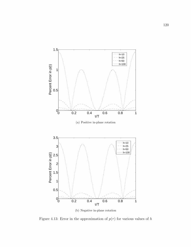
120

0 0.2 0.4 0.6 0.8 10

0.5

1

1.5

τ/T

Per

cent

Err

or in

p(τ

)

h=10h=25h=50h=100

(a) Positive in-plane rotation

0 0.2 0.4 0.6 0.8 10

0.5

1

1.5

2

2.5

3

3.5

τ/T

Per

cent

Err

or in

p(τ

)

h=10h=25h=50h=100

(b) Negative in-plane rotation

Figure 4.13: Error in the approximation of p(τ) for various values of h

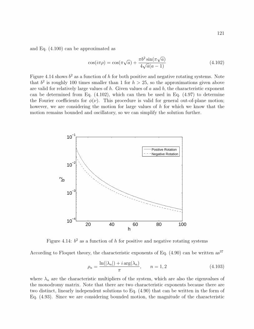
121

and Eq. (4.100) can be approximated as

cos(iπρ) = cos(π√a) +

πb2 sin(π√a)

4√a(a− 1)

(4.102)

Figure 4.14 shows b2 as a function of h for both positive and negative rotating systems. Notethat b2 is roughly 100 times smaller than 1 for h > 25, so the approximations given aboveare valid for relatively large values of h. Given values of a and b, the characteristic exponentcan be determined from Eq. (4.102), which can then be used in Eq. (4.97) to determinethe Fourier coefficients for φ(ν). This procedure is valid for general out-of-plane motion;however, we are considering the motion for large values of h for which we know that themotion remains bounded and oscillatory, so we can simplify the solution further.

20 40 60 80 10010

−4

10−3

10−2

10−1

h

b2

Positive RotationNegative Rotation

Figure 4.14: b2 as a function of h for positive and negative rotating systems

According to Floquet theory, the characteristic exponents of Eq. (4.90) can be written as37

ρn =ln(|λn|) + i arg(λn)

π, n = 1, 2 (4.103)

where λn are the characteristic multipliers of the system, which are also the eigenvalues ofthe monodromy matrix. Note that there are two characteristic exponents because there aretwo distinct, linearly independent solutions to Eq. (4.90) that can be written in the form ofEq. (4.93). Since we are considering bounded motion, the magnitude of the characteristic

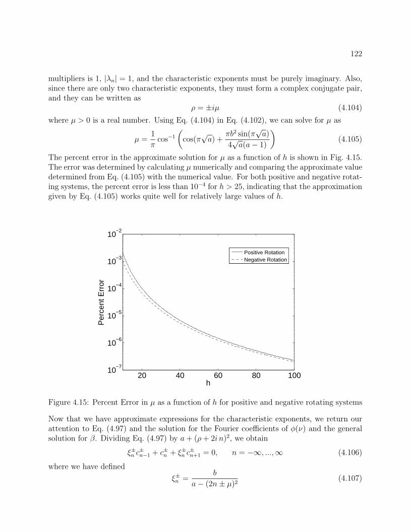
122

multipliers is 1, |λn| = 1, and the characteristic exponents must be purely imaginary. Also,since there are only two characteristic exponents, they must form a complex conjugate pair,and they can be written as

ρ = ±iµ (4.104)

where µ > 0 is a real number. Using Eq. (4.104) in Eq. (4.102), we can solve for µ as

µ =1

πcos−1

(cos(π

√a) +

πb2 sin(π√a)

4√a(a− 1)

)(4.105)

The percent error in the approximate solution for µ as a function of h is shown in Fig. 4.15.The error was determined by calculating µ numerically and comparing the approximate valuedetermined from Eq. (4.105) with the numerical value. For both positive and negative rotat-ing systems, the percent error is less than 10−4 for h > 25, indicating that the approximationgiven by Eq. (4.105) works quite well for relatively large values of h.

20 40 60 80 10010

−7

10−6

10−5

10−4

10−3

10−2

h

Per

cent

Err

or

Positive RotationNegative Rotation

Figure 4.15: Percent Error in µ as a function of h for positive and negative rotating systems

Now that we have approximate expressions for the characteristic exponents, we return ourattention to Eq. (4.97) and the solution for the Fourier coefficients of φ(ν) and the generalsolution for β. Dividing Eq. (4.97) by a+ (ρ+ 2i n)2, we obtain

ξ±n c±n−1 + c±n + ξ±n c

±n+1 = 0, n = −∞, ...,∞ (4.106)


ξ±n =b

a− (2n± µ)2(4.107)

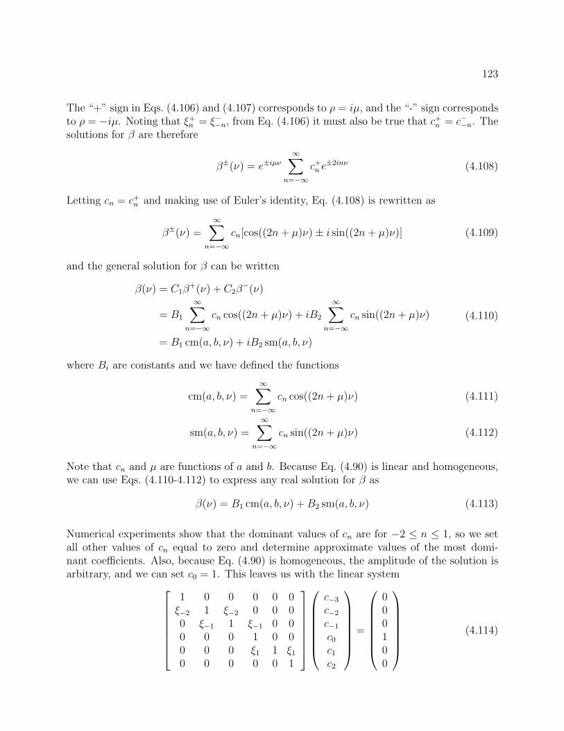
123

The “+” sign in Eqs. (4.106) and (4.107) corresponds to ρ = iµ, and the “-” sign correspondsto ρ = −iµ. Noting that ξ+

n = ξ−−n, from Eq. (4.106) it must also be true that c+n = c−−n. The

solutions for β are therefore

β±(ν) = e±iµν∞∑

n=−∞

c+n e±2inν (4.108)

Letting cn = c+n and making use of Euler’s identity, Eq. (4.108) is rewritten as

β±(ν) =∞∑

n=−∞

cn[cos((2n+ µ)ν)± i sin((2n+ µ)ν)] (4.109)

and the general solution for β can be written

β(ν) = C1β+(ν) + C2β

−(ν)

= B1

∞∑n=−∞

cn cos((2n+ µ)ν) + iB2

∞∑n=−∞

cn sin((2n+ µ)ν)

= B1 cm(a, b, ν) + iB2 sm(a, b, ν)

(4.110)

where Bi are constants and we have defined the functions

cm(a, b, ν) =∞∑

n=−∞

cn cos((2n+ µ)ν) (4.111)

sm(a, b, ν) =∞∑

n=−∞

cn sin((2n+ µ)ν) (4.112)

Note that cn and µ are functions of a and b. Because Eq. (4.90) is linear and homogeneous,we can use Eqs. (4.110-4.112) to express any real solution for β as

β(ν) = B1 cm(a, b, ν) +B2 sm(a, b, ν) (4.113)

Numerical experiments show that the dominant values of cn are for −2 ≤ n ≤ 1, so we setall other values of cn equal to zero and determine approximate values of the most domi-nant coefficients. Also, because Eq. (4.90) is homogeneous, the amplitude of the solution isarbitrary, and we can set c0 = 1. This leaves us with the linear system

1 0 0 0 0 0ξ−2 1 ξ−2 0 0 00 ξ−1 1 ξ−1 0 00 0 0 1 0 00 0 0 ξ1 1 ξ1

0 0 0 0 0 1

c−3

c−2

c−1

c0

c1

c2

=

000100

(4.114)

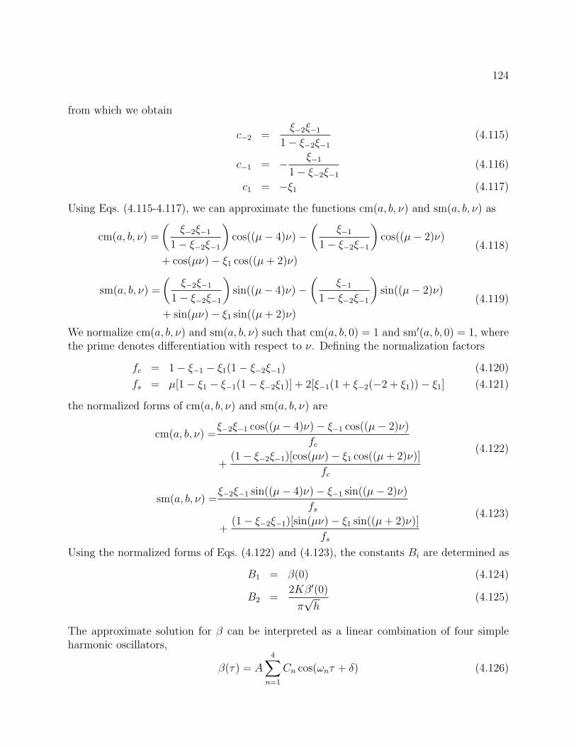
124

from which we obtain

c−2 =ξ−2ξ−1

1− ξ−2ξ−1

(4.115)

c−1 = − ξ−1

1− ξ−2ξ−1

(4.116)

c1 = −ξ1 (4.117)

Using Eqs. (4.115-4.117), we can approximate the functions cm(a, b, ν) and sm(a, b, ν) as

cm(a, b, ν) =

(ξ−2ξ−1

1− ξ−2ξ−1

)cos((µ− 4)ν)−

(ξ−1

1− ξ−2ξ−1

)cos((µ− 2)ν)

+ cos(µν)− ξ1 cos((µ+ 2)ν)

(4.118)

sm(a, b, ν) =

(ξ−2ξ−1

1− ξ−2ξ−1

)sin((µ− 4)ν)−

(ξ−1

1− ξ−2ξ−1

)sin((µ− 2)ν)

+ sin(µν)− ξ1 sin((µ+ 2)ν)

(4.119)

We normalize cm(a, b, ν) and sm(a, b, ν) such that cm(a, b, 0) = 1 and sm′(a, b, 0) = 1, wherethe prime denotes differentiation with respect to ν. Defining the normalization factors

fc = 1− ξ−1 − ξ1(1− ξ−2ξ−1) (4.120)

fs = µ[1− ξ1 − ξ−1(1− ξ−2ξ1)] + 2[ξ−1(1 + ξ−2(−2 + ξ1))− ξ1] (4.121)

the normalized forms of cm(a, b, ν) and sm(a, b, ν) are

cm(a, b, ν) =ξ−2ξ−1 cos((µ− 4)ν)− ξ−1 cos((µ− 2)ν)

fc

+(1− ξ−2ξ−1)[cos(µν)− ξ1 cos((µ+ 2)ν)]

fc

(4.122)

sm(a, b, ν) =ξ−2ξ−1 sin((µ− 4)ν)− ξ−1 sin((µ− 2)ν)

fs

+(1− ξ−2ξ−1)[sin(µν)− ξ1 sin((µ+ 2)ν)]

fs

(4.123)

Using the normalized forms of Eqs. (4.122) and (4.123), the constants Bi are determined as

B1 = β(0) (4.124)

B2 =2Kβ′(0)

π√h

(4.125)

The approximate solution for β can be interpreted as a linear combination of four simpleharmonic oscillators,

β(τ) = A

4∑n=1

Cn cos(ωnτ + δ) (4.126)

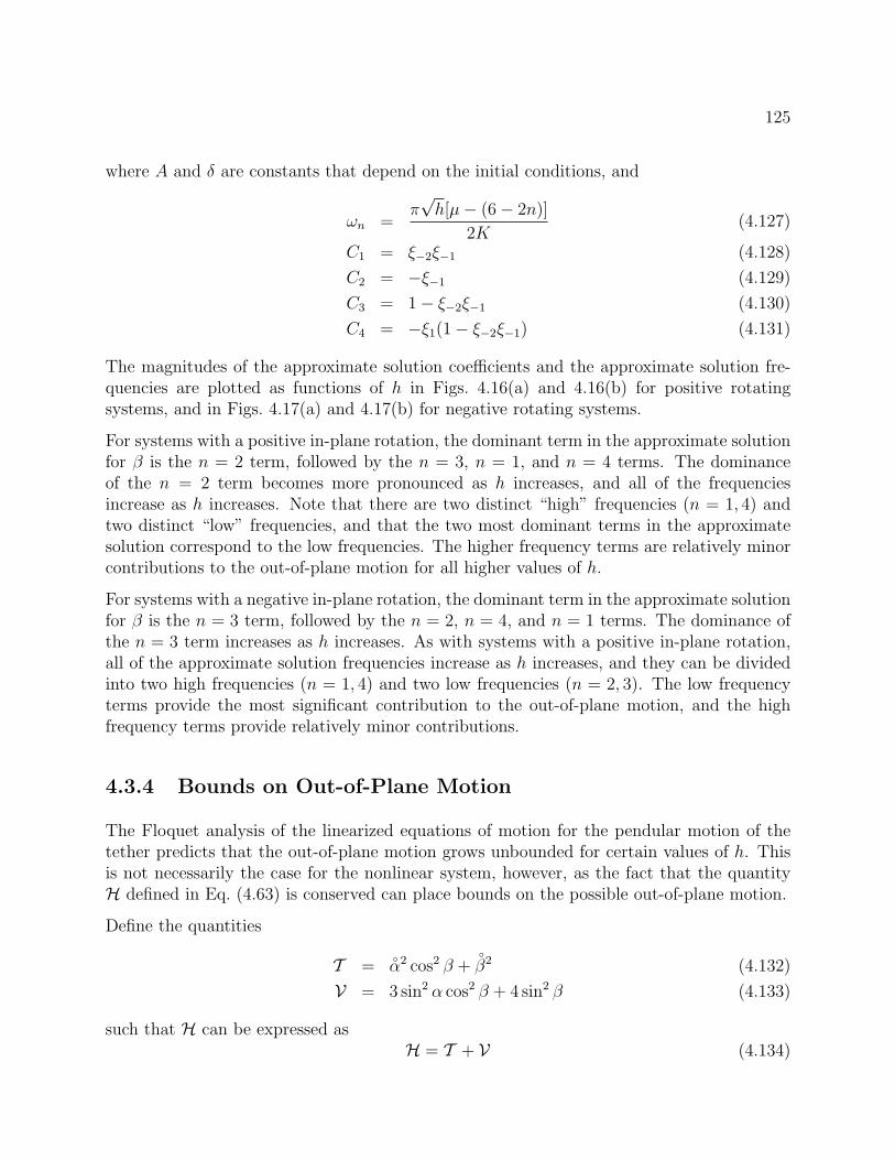
125

where A and δ are constants that depend on the initial conditions, and

ωn =π√h[µ− (6− 2n)]

2K(4.127)

C1 = ξ−2ξ−1 (4.128)

C2 = −ξ−1 (4.129)

C3 = 1− ξ−2ξ−1 (4.130)

C4 = −ξ1(1− ξ−2ξ−1) (4.131)

The magnitudes of the approximate solution coefficients and the approximate solution fre-quencies are plotted as functions of h in Figs. 4.16(a) and 4.16(b) for positive rotatingsystems, and in Figs. 4.17(a) and 4.17(b) for negative rotating systems.

For systems with a positive in-plane rotation, the dominant term in the approximate solutionfor β is the n = 2 term, followed by the n = 3, n = 1, and n = 4 terms. The dominanceof the n = 2 term becomes more pronounced as h increases, and all of the frequenciesincrease as h increases. Note that there are two distinct “high” frequencies (n = 1, 4) andtwo distinct “low” frequencies, and that the two most dominant terms in the approximatesolution correspond to the low frequencies. The higher frequency terms are relatively minorcontributions to the out-of-plane motion for all higher values of h.

For systems with a negative in-plane rotation, the dominant term in the approximate solutionfor β is the n = 3 term, followed by the n = 2, n = 4, and n = 1 terms. The dominance ofthe n = 3 term increases as h increases. As with systems with a positive in-plane rotation,all of the approximate solution frequencies increase as h increases, and they can be dividedinto two high frequencies (n = 1, 4) and two low frequencies (n = 2, 3). The low frequencyterms provide the most significant contribution to the out-of-plane motion, and the highfrequency terms provide relatively minor contributions.

4.3.4 Bounds on Out-of-Plane Motion

The Floquet analysis of the linearized equations of motion for the pendular motion of thetether predicts that the out-of-plane motion grows unbounded for certain values of h. Thisis not necessarily the case for the nonlinear system, however, as the fact that the quantityH defined in Eq. (4.63) is conserved can place bounds on the possible out-of-plane motion.

Define the quantities

T =α2 cos2 β +

β2 (4.132)

V = 3 sin2 α cos2 β + 4 sin2 β (4.133)

such that H can be expressed asH = T + V (4.134)

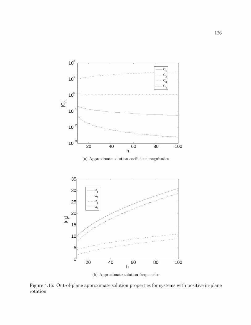
126

20 40 60 80 10010

−3

10−2

10−1

100

101

102

h

|Cn|

C

1

C2

C3

C4

(a) Approximate solution coefficient magnitudes

20 40 60 80 1000

5

10

15

20

25

30

35

h

|ωn|

ω1

ω2

ω3

ω4

(b) Approximate solution frequencies

Figure 4.16: Out-of-plane approximate solution properties for systems with positive in-planerotation

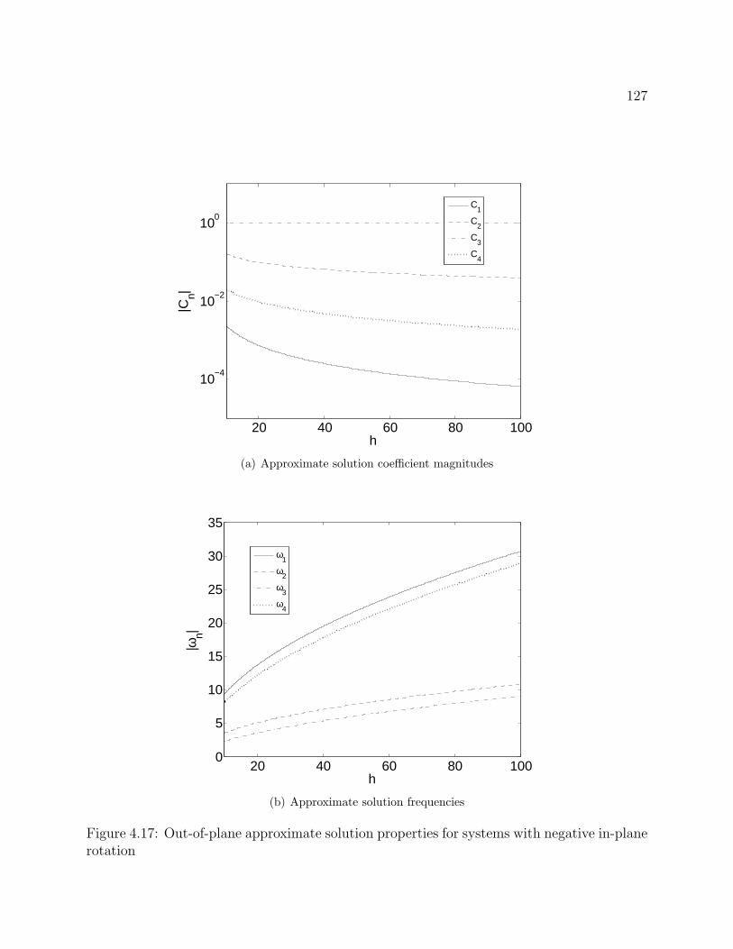
127

20 40 60 80 100

10−4

10−2

100

h

|Cn|

C

1

C2

C3

C4

(a) Approximate solution coefficient magnitudes

20 40 60 80 1000

5

10

15

20

25

30

35

h

|ωn|

ω1

ω2

ω3

ω4

(b) Approximate solution frequencies

Figure 4.17: Out-of-plane approximate solution properties for systems with negative in-planerotation

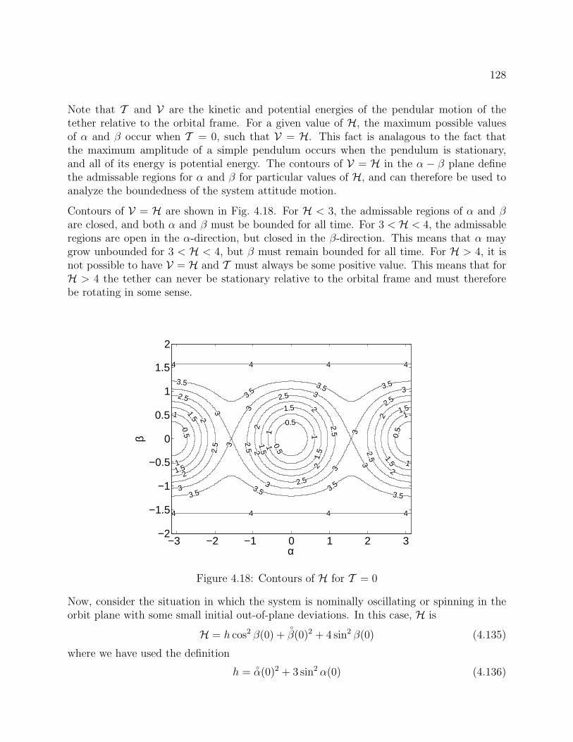
128

Note that T and V are the kinetic and potential energies of the pendular motion of thetether relative to the orbital frame. For a given value of H, the maximum possible valuesof α and β occur when T = 0, such that V = H. This fact is analagous to the fact thatthe maximum amplitude of a simple pendulum occurs when the pendulum is stationary,and all of its energy is potential energy. The contours of V = H in the α − β plane definethe admissable regions for α and β for particular values of H, and can therefore be used toanalyze the boundedness of the system attitude motion.

Contours of V = H are shown in Fig. 4.18. For H < 3, the admissable regions of α and βare closed, and both α and β must be bounded for all time. For 3 < H < 4, the admissableregions are open in the α-direction, but closed in the β-direction. This means that α maygrow unbounded for 3 < H < 4, but β must remain bounded for all time. For H > 4, it isnot possible to have V = H and T must always be some positive value. This means that forH > 4 the tether can never be stationary relative to the orbital frame and must thereforebe rotating in some sense.

0.5 0.5

0.5

0.51

1

1

1

1

11

1.5

1.5

1.5

1.5

1.51.

5

1.5

2

2

2

2

22

22

2.5

2.5

2.5

2.5

2.5

2.5

2.5

2.5

3 3

3

3

3

3

3

3

3

3

3.5

3.53.5 3.5

3.53.5 3.5

3.5

4 4 4 4

4 4 4 4

α

β

−3 −2 −1 0 1 2 3−2

−1.5

−1

−0.5

0

0.5

1

1.5

2

Figure 4.18: Contours of H for T = 0

Now, consider the situation in which the system is nominally oscillating or spinning in theorbit plane with some small initial out-of-plane deviations. In this case, H is

H = h cos2 β(0) +β(0)2 + 4 sin2 β(0) (4.135)

where we have used the definition

h =α(0)2 + 3 sin2 α(0) (4.136)

129

because the pendular motion is ideally planar with energy level h, but there are small initialout-of-plane deviations. The out-of-plane motion must remain bounded if H < 4, in whichcase the maximum possible value of β is

βmax = sin−1

√h cos2 β(0) +

β(0)2 + 4 sin2 β(0)

2

(4.137)

Since we are assuming that the initial out-of-plane deviations are small, we can approximateβmax as

βmax ≈ sin−1

(√h

2

)(4.138)

So, for h > 4 it is possible for small initial out-of-plane deviations to grow unbounded,but for h < 4 the out-of-plane motion must remain bounded. As indicated by the Floquetanalysis, the out-of-plane motion can grow quite large, but it must remain bounded for h < 4.This means that the out-of-plane motion will not grow unbounded in the unstable regionsdiscovered previously in this section for systems with a positive in-plane rotation.

4.3.5 Summary of Computational Predictions

In this section we presented aspects of the lower-level computational model pertaining to thependular motion of the tether. Because the nominal pendular motion of the tether is a planar

spin, the equations governing the pendular motion were linearized about β =β = 0 and the

solution for the in-plane motion was determined analytically. This solution was then usedin the equation governing the out-of-plane motion, resulting in a Hill’s equation. Floquettheory was used to show that this equation is unstable for certain in plane spin rates, meaningthat the lower-level computational model predicts unstable out-of-plane motion for somecases. The out-of-plane motion does not grow unbounded, however, due to the fact that theequations governing the pendular motion are conservative. This fact was used to determineapproximate bounds on the out-of-plane motion for unstable cases. For relatively high in-plane spin rates the Hill’s equation governing the small out-of-plane motion is accuratelyapproximated by a Mathieu’s equation for which approximate solutions were determined.These approximate solutions take the form of linear combinations of four simple harmonicoscillators, each with a different oscillation frequency and relative magnitude. Later in thischapter, many of the results derived in this section using the lower-level system model arecompared to numerical solutions determined using the top-level computational model for thepurposes of validation.

130

4.4 Computational Model: Transverse Vibrations of

the Tether

In this section we develop several aspects of the lower-level computational model related tothe transverse vibrations of the tether. The analysis of the transverse vibrations makes useof some of the results related to the tether pendular motion presented in the previous section,and many of the analysis methods that we apply to the transverse vibrations are similar tothose applied to the pendular motion. Unlike the results presented in the previous section,the analytical results related to the tether transverse vibrations presented in this section arenot original contributions, in that they duplicate the results presented in Refs. [5] and [8].The original contribution related to the tether transverse vibrations is provided in the nextsection in which the top-level computational model is used to perform validation tests onthe results presented in this section.

4.4.1 Analysis Using Separation of Variables

As done in the analysis of the pendular motion of the tether, we assume that the out-of-plane pendular motion is small. In addition, we assume that the transverse vibrations of thetether are small relative to the length of the tether, such that u and v are small quantities.Combining these assumptions, the equations of motion of the tether transverse vibrationssimplify to

u− [(

α + 1)2 + 3 sin2 α− 1]u = [(

α + 1)2 + 3 cos2 α− 1]

[(2− γx2

2γ

)u′′ − xu′

](4.139)

v + v = [(

α + 1)2 + 3 cos2 α− 1]

[(2− γx2

2γ

)v′′ − xv′

](4.140)

Note that because we assume that β is small, the solution for α is given by Eqs. (4.69) and(4.70).

To analyze Eqs. (4.139) and (4.140) we apply the principle of separation of variables.7 As-sume solutions for u and v of the form

u(x, τ) = Xu(x)Fu(τ) (4.141)

v(x, τ) = Xv(x)Fv(τ) (4.142)

where Xu and Xv are spatially-dependent mode shapes, and Fu and Fv are time-dependentfunctions. Using Eq. (4.141) in Eq. (4.140), we find that Xu and Fu must satisfy

Fu − [(

α + 1)2 + 3 sin2 α− 1]Fu

[(α + 1)2 + 3 cos2 α− 1]Fu

=1

Xu

[(2− γx2

2γ

)X ′′u − xX ′u

](4.143)

131

The left-hand side of Eq. (4.143) is a function of τ only, and the right-hand side is a functionof x only. Because Eq. (4.143) must hold for all τ and x, both sides of the expression mustbe equal to the same constant, which we denote −λu,

Fu − [(

α + 1)2 + 3 sin2 α− 1]Fu

[(α + 1)2 + 3 cos2 α− 1]Fu

=1

Xu

[(2− γx2

2γ

)X ′′u − xX ′u

]= −λu (4.144)

From this point forward we refer to the constant λu as an eigenvalue of Eq. (4.139). UsingEq. (4.141) in the boundary conditions for u, we obtain

Xu(0)Fu(τ) = Xu(1)Fu(τ) = 0 (4.145)

which must hold for all τ . From Eqs. (4.144) and (4.145), the mode shape Xu must satisfythe boundary value problem

(2− γx2)X ′′u − 2γxX ′u + 2γλuXu = 0 (4.146)

Xu(0) = Xu(1) = 0 (4.147)

Note that Eq. (4.146) is a nonstandard form of the Legendre differential equation.7 FromEq. (4.144), the function Fu must satisfy the differential equation

Fu + [(λu − 1)(

α + 1)2 + (λu + 1)(3 cos2 α− 1)− 1]Fu = 0 (4.148)

Using Eq. (4.142) in Eq. (4.140) and following the procedure illustrated above, we find thatthe mode shape Xv must satisfy the boundary value problem

(2− γx2)X ′′v − 2γxX ′v + 2γλvXv = 0 (4.149)

Xv(0) = Xv(1) = 0 (4.150)

and the function Fv must satisfy the differential equation

Fv + [λv(

α + 1)2 + λv(3 cos2 α− 1) + 1]Fv = 0 (4.151)

Note that the constant λv in Eqs. (4.149) and (4.151) is an eigenvalue of Eq. (4.140).

Comparing Eqs. (4.146) and (4.147) with Eqs. (4.149) and (4.150) we see that the modeshapes for u and v are governed by the same boundary value problem. Without loss ofgenerality, we can therefore define X(x) = Xu(x) = Xv(x) and λ = λu = λv, such that themode shapes for the transverse vibrations are governed by

(2− γx2)X ′′ − 2γxX ′ + 2γλX = 0 (4.152)

X(0) = X(1) = 0 (4.153)

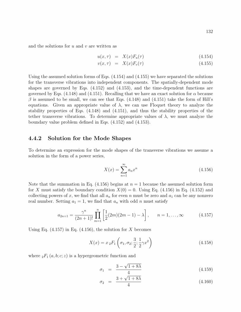
132

and the solutions for u and v are written as

u(x, τ) = X(x)Fu(τ) (4.154)

v(x, τ) = X(x)Fv(τ) (4.155)

Using the assumed solution forms of Eqs. (4.154) and (4.155) we have separated the solutionsfor the transverse vibrations into independent components. The spatially-dependent modeshapes are governed by Eqs. (4.152) and (4.153), and the time-dependent functions aregoverned by Eqs. (4.148) and (4.151). Recalling that we have an exact solution for α becauseβ is assumed to be small, we can see that Eqs. (4.148) and (4.151) take the form of Hill’sequations. Given an appropriate value of λ, we can use Floquet theory to analyze thestability properties of Eqs. (4.148) and (4.151), and thus the stability properties of thetether transverse vibrations. To determine appropriate values of λ, we must analyze theboundary value problem defined in Eqs. (4.152) and (4.153).

4.4.2 Solution for the Mode Shapes

To determine an expression for the mode shapes of the transverse vibrations we assume asolution in the form of a power series,

X(x) =∞∑n=1

anxn (4.156)

Note that the summation in Eq. (4.156) begins at n = 1 because the assumed solution formfor X must satisfy the boundary condition X(0) = 0. Using Eq. (4.156) in Eq. (4.152) andcollecting powers of x, we find that all an for even n must be zero and a1 can be any nonzeroreal number. Setting a1 = 1, we find that an with odd n must satisfy

a2n+1 =γn

(2n+ 1)!

n∏m=1

[1

2(2m)(2m− 1)− λ

], n = 1, . . . ,∞ (4.157)

Using Eq. (4.157) in Eq. (4.156), the solution for X becomes

X(x) = x 2F1

(σ1, σ2;

3

2;1

2γx2

)(4.158)

where 2F1 (a, b; c; z) is a hypergeometric function and

σ1 =3−√

1 + 8λ

4(4.159)

σ2 =3 +√

1 + 8λ

4(4.160)

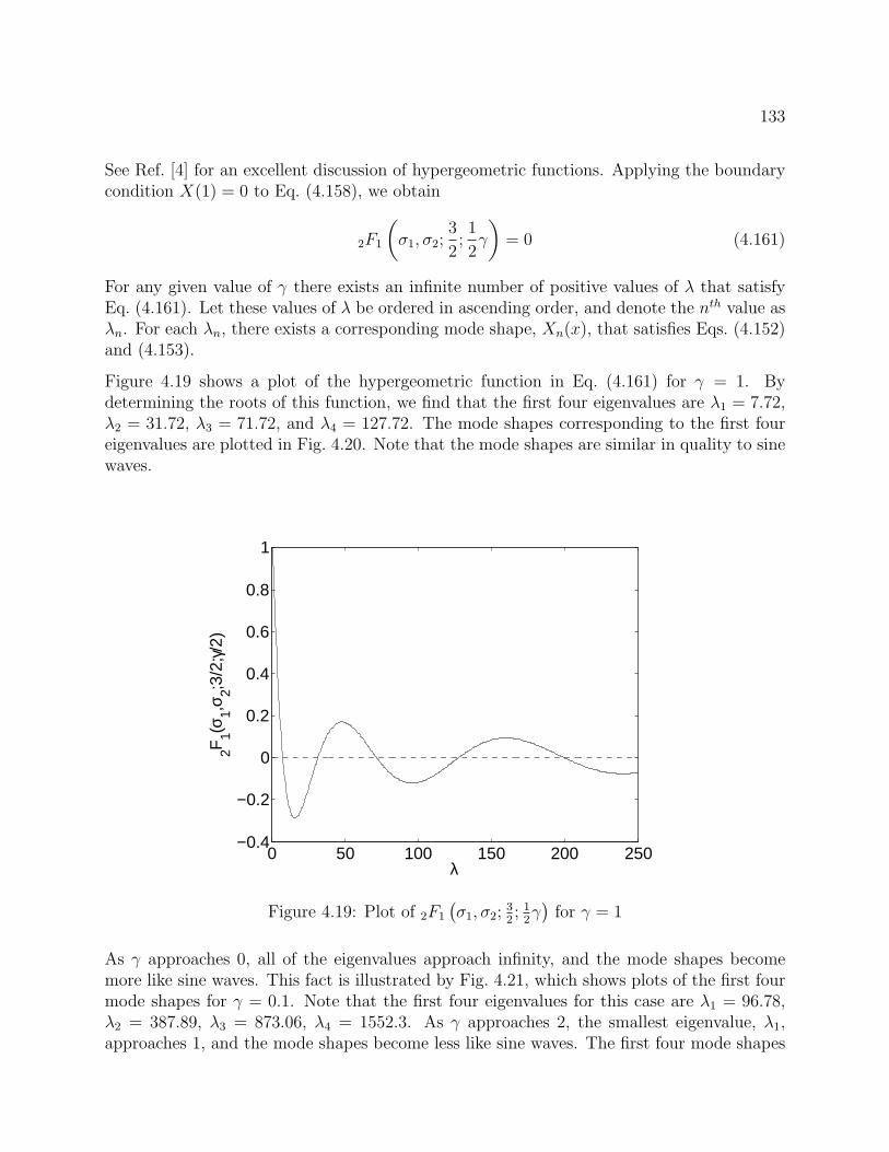
133

See Ref. [4] for an excellent discussion of hypergeometric functions. Applying the boundarycondition X(1) = 0 to Eq. (4.158), we obtain

2F1

(σ1, σ2;

3

2;1

2γ

)= 0 (4.161)

For any given value of γ there exists an infinite number of positive values of λ that satisfyEq. (4.161). Let these values of λ be ordered in ascending order, and denote the nth value asλn. For each λn, there exists a corresponding mode shape, Xn(x), that satisfies Eqs. (4.152)and (4.153).

Figure 4.19 shows a plot of the hypergeometric function in Eq. (4.161) for γ = 1. Bydetermining the roots of this function, we find that the first four eigenvalues are λ1 = 7.72,λ2 = 31.72, λ3 = 71.72, and λ4 = 127.72. The mode shapes corresponding to the first foureigenvalues are plotted in Fig. 4.20. Note that the mode shapes are similar in quality to sinewaves.

0 50 100 150 200 250−0.4

−0.2

0

0.2

0.4

0.6

0.8

1

λ

2F1(σ

1,σ2;3

/2;γ/

2)

Figure 4.19: Plot of 2F1

(σ1, σ2; 3

2; 1

2γ)

for γ = 1

As γ approaches 0, all of the eigenvalues approach infinity, and the mode shapes becomemore like sine waves. This fact is illustrated by Fig. 4.21, which shows plots of the first fourmode shapes for γ = 0.1. Note that the first four eigenvalues for this case are λ1 = 96.78,λ2 = 387.89, λ3 = 873.06, λ4 = 1552.3. As γ approaches 2, the smallest eigenvalue, λ1,approaches 1, and the mode shapes become less like sine waves. The first four mode shapes

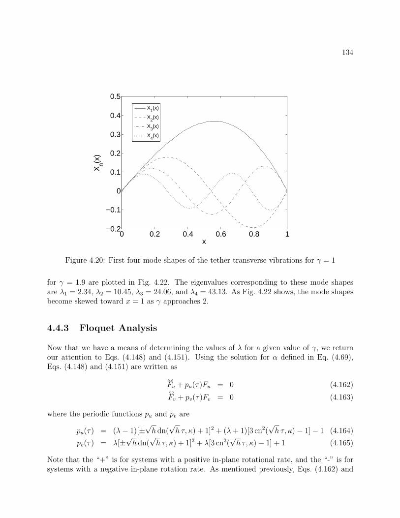
134

0 0.2 0.4 0.6 0.8 1−0.2

−0.1

0

0.1

0.2

0.3

0.4

0.5

x

Xn(x

)

X

1(x)

X2(x)

X3(x)

X4(x)

Figure 4.20: First four mode shapes of the tether transverse vibrations for γ = 1

for γ = 1.9 are plotted in Fig. 4.22. The eigenvalues corresponding to these mode shapesare λ1 = 2.34, λ2 = 10.45, λ3 = 24.06, and λ4 = 43.13. As Fig. 4.22 shows, the mode shapesbecome skewed toward x = 1 as γ approaches 2.

4.4.3 Floquet Analysis

Now that we have a means of determining the values of λ for a given value of γ, we returnour attention to Eqs. (4.148) and (4.151). Using the solution for α defined in Eq. (4.69),Eqs. (4.148) and (4.151) are written as

Fu + pu(τ)Fu = 0 (4.162)Fv + pv(τ)Fv = 0 (4.163)

where the periodic functions pu and pv are

pu(τ) = (λ− 1)[±√h dn(

√h τ, κ) + 1]2 + (λ+ 1)[3 cn2(

√h τ, κ)− 1]− 1 (4.164)

pv(τ) = λ[±√h dn(

√h τ, κ) + 1]2 + λ[3 cn2(

√h τ, κ)− 1] + 1 (4.165)

Note that the “+” is for systems with a positive in-plane rotational rate, and the “-” is forsystems with a negative in-plane rotation rate. As mentioned previously, Eqs. (4.162) and

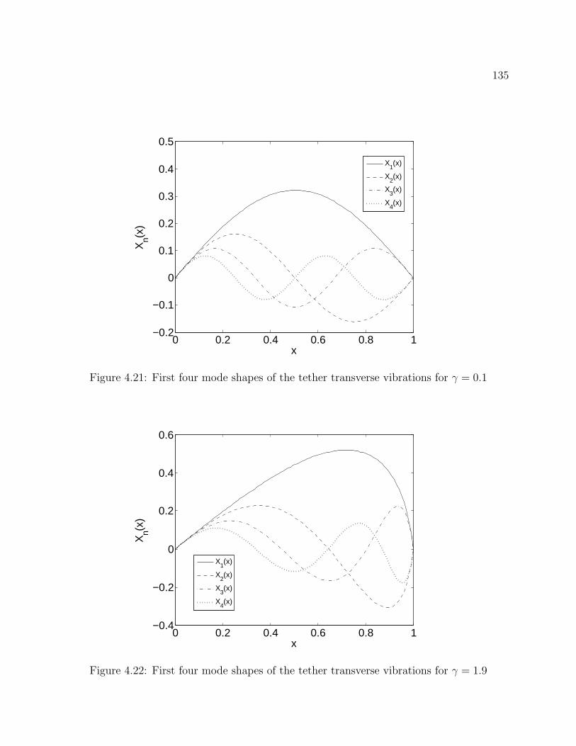
135

0 0.2 0.4 0.6 0.8 1−0.2

−0.1

0

0.1

0.2

0.3

0.4

0.5

x

Xn(x

)

X1(x)

X2(x)

X3(x)

X4(x)

Figure 4.21: First four mode shapes of the tether transverse vibrations for γ = 0.1

0 0.2 0.4 0.6 0.8 1−0.4

−0.2

0

0.2

0.4

0.6

x

Xn(x

)

X1(x)

X2(x)

X3(x)

X4(x)

Figure 4.22: First four mode shapes of the tether transverse vibrations for γ = 1.9

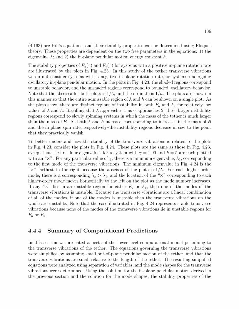
136

(4.163) are Hill’s equations, and their stability properties can be determined using Floquettheory. These properties are dependent on the two free parameters in the equations: 1) theeigenvalue λ; and 2) the in-plane pendular motion energy constant h.

The stability properties of Fu(τ) and Fv(τ) for systems with a positive in-plane rotation rateare illustrated by the plots in Fig. 4.23. In this study of the tether transverse vibrationswe do not consider systems with a negative in-plane rotation rate, or systems undergoingoscillatory in-plane pendular motion. In the plots in Fig. 4.23, the shaded regions correspondto unstable behavior, and the unshaded regions correspond to bounded, oscillatory behavior.Note that the abscissa for both plots is 1/λ, and the ordinate is 1/h. The plots are shown inthis manner so that the entire admissable region of λ and h can be shown on a single plot. Asthe plots show, there are distinct regions of instability in both Fu and Fv for relatively lowvalues of λ and h. Recalling that λ approaches 1 as γ approaches 2, these larger instabilityregions correspond to slowly spinning systems in which the mass of the tether is much largerthan the mass of B. As both λ and h increase–corresponding to increases in the mass of Band the in-plane spin rate, respectively–the instability regions decrease in size to the pointthat they practically vanish.

To better understand how the stability of the transverse vibrations is related to the plotsin Fig. 4.23, consider the plots in Fig. 4.24. These plots are the same as those in Fig. 4.23,except that the first four eigenvalues for a system with γ = 1.99 and h = 5 are each plottedwith an “×”. For any particular value of γ, there is a minimum eigenvalue, λ1, correspondingto the first mode of the transverse vibrations. The minimum eigenvalue in Fig. 4.24 is the“×” farthest to the right because the abscissa of the plots is 1/λ. For each higher-ordermode, there is a corresponding λn > λ1, and the location of the “×” corresponding to eachhigher-order mode moves horizontally to the left on the plot as the mode number increases.If any “×” lies in an unstable region for either Fu or Fv, then one of the modes of thetransverse vibrations is unstable. Because the transverse vibrations are a linear combinationof all of the modes, if one of the modes is unstable then the transverse vibrations on thewhole are unstable. Note that the case illustrated in Fig. 4.24 represents stable transversevibrations because none of the modes of the transverse vibrations lie in unstable regions forFu or Fv.

4.4.4 Summary of Computational Predictions

In this section we presented aspects of the lower-level computational model pertaining tothe transverse vibrations of the tether. The equations governing the transverse vibrationswere simplified by assuming small out-of-plane pendular motion of the tether, and that thetransverse vibrations are small relative to the length of the tether. The resulting simplifiedequations were analyzed using separation of variables, and the mode shapes for the transversevibrations were determined. Using the solution for the in-plane pendular motion derived inthe previous section and the solution for the mode shapes, the stability properties of the

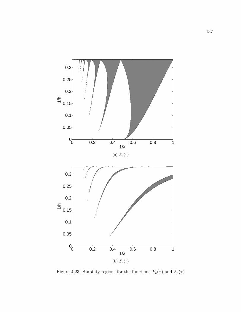
137

0 0.2 0.4 0.6 0.8 10

0.05

0.1

0.15

0.2

0.25

0.3

1/λ

1/h

(a) Fu(τ)

0 0.2 0.4 0.6 0.8 10

0.05

0.1

0.15

0.2

0.25

0.3

1/λ

1/h

(b) Fv(τ)

Figure 4.23: Stability regions for the functions Fu(τ) and Fv(τ)

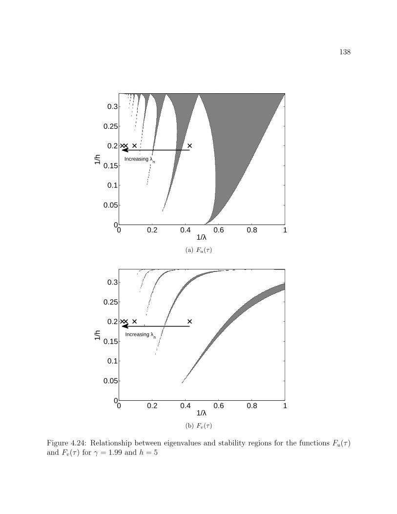
138

0 0.2 0.4 0.6 0.8 10

0.05

0.1

0.15

0.2

0.25

0.3

1/λ

1/h Increasing λ

n

(a) Fu(τ)

0 0.2 0.4 0.6 0.8 10

0.05

0.1

0.15

0.2

0.25

0.3

1/λ

1/h Increasing λ

n

(b) Fv(τ)

Figure 4.24: Relationship between eigenvalues and stability regions for the functions Fu(τ)and Fv(τ) for γ = 1.99 and h = 5

139

transverse vibrations were analyzed using Floquet theory.

The lower-level computational model predicts distinct regions of transverse vibration insta-bility for certain types of systems. The largest regions of instability correspond to systemswith relatively low values of λ and h. A low value of h means that the in-plane spin rate isrelatively low, which could apply to any type of spinning TSS. Low values of λ correspondto systems with values of γ near 2 because λ1 approaches 1 as γ approaches 2, and λ1 isthe minumum eigenvalue for a given value of γ. As mentioned previously, a γ near 2 meansthat the mass of the tether is much greater than the mass of B, so the lower-level compu-tational model predicts that these types of systems have the largest range of configurationsthat experience unstable transverse vibrations. As both λ and h increase, the instabilityregions decrease in size and become virtually nonexistent. This means that the lower-levelcomputational model predicts that systems with a relatively high in-plane spin rate and largesecondary end body mass will practically never experience unstable transverse vibrations. Inthe next section, we use numerical solutions determined using the top-level computationalmodel to perform validation tests on these results related to the stability of the transversevibrations of the tether.

4.5 Validation of the Computational Model

In §4.3 and §4.4 we developed several elements of the lower-level computational model relatedto the dynamics of the tether in a spinning TSS. Specifically, we showed that the lower-levelmodel predicts that both the pendular motion and elastic vibrations of the tether are unsta-ble for certain system configurations, and we also determined approximate solutions for theout-of-plane pendular motion for systems with a relatively high in-plane spin rate. In thissection we apply the model validation procedure outlined in Ch. 2 to these computationalpredictions. For any results that are not validated through the application of this proce-dure, we perform an analysis of the modeling assumptions used in the lower-level model todetermine how the model should be altered to produce better agreement with the top-levelcomputational model.

4.5.1 Pendular Motion of the Tether

The lower-level computational model predicts that the out-of-plane pendular motion of thetether is unstable for certain ranges of the the parameter h, which is a measure of theenergy of the in-plane pendular motion. For relatively large values of h, the out-of-planependular motion is predicted to be stable and oscillatory, and approximate solutions for theout-of-plane motion can be expressed as finite sums of simple harmonic oscillators. Thesecomputational predictions are now compared to the top-level computational model for thepurposes of validation; however, validation tests are only performed on the results that are

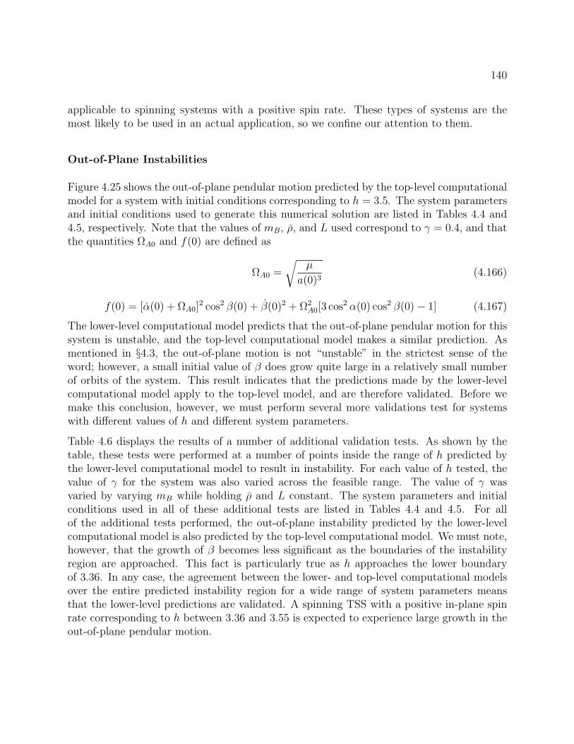
140

applicable to spinning systems with a positive spin rate. These types of systems are themost likely to be used in an actual application, so we confine our attention to them.

Out-of-Plane Instabilities

Figure 4.25 shows the out-of-plane pendular motion predicted by the top-level computationalmodel for a system with initial conditions corresponding to h = 3.5. The system parametersand initial conditions used to generate this numerical solution are listed in Tables 4.4 and4.5, respectively. Note that the values of mB, ρ, and L used correspond to γ = 0.4, and thatthe quantities ΩA0 and f(0) are defined as

ΩA0 =

√µ

a(0)3(4.166)

f(0) = [α(0) + ΩA0]2 cos2 β(0) + β(0)2 + Ω2A0[3 cos2 α(0) cos2 β(0)− 1] (4.167)

The lower-level computational model predicts that the out-of-plane pendular motion for thissystem is unstable, and the top-level computational model makes a similar prediction. Asmentioned in §4.3, the out-of-plane motion is not “unstable” in the strictest sense of theword; however, a small initial value of β does grow quite large in a relatively small numberof orbits of the system. This result indicates that the predictions made by the lower-levelcomputational model apply to the top-level model, and are therefore validated. Before wemake this conclusion, however, we must perform several more validations test for systemswith different values of h and different system parameters.

Table 4.6 displays the results of a number of additional validation tests. As shown by thetable, these tests were performed at a number of points inside the range of h predicted bythe lower-level computational model to result in instability. For each value of h tested, thevalue of γ for the system was also varied across the feasible range. The value of γ wasvaried by varying mB while holding ρ and L constant. The system parameters and initialconditions used in all of these additional tests are listed in Tables 4.4 and 4.5. For allof the additional tests performed, the out-of-plane instability predicted by the lower-levelcomputational model is also predicted by the top-level computational model. We must note,however, that the growth of β becomes less significant as the boundaries of the instabilityregion are approached. This fact is particularly true as h approaches the lower boundaryof 3.36. In any case, the agreement between the lower- and top-level computational modelsover the entire predicted instability region for a wide range of system parameters meansthat the lower-level predictions are validated. A spinning TSS with a positive in-plane spinrate corresponding to h between 3.36 and 3.55 is expected to experience large growth in theout-of-plane pendular motion.

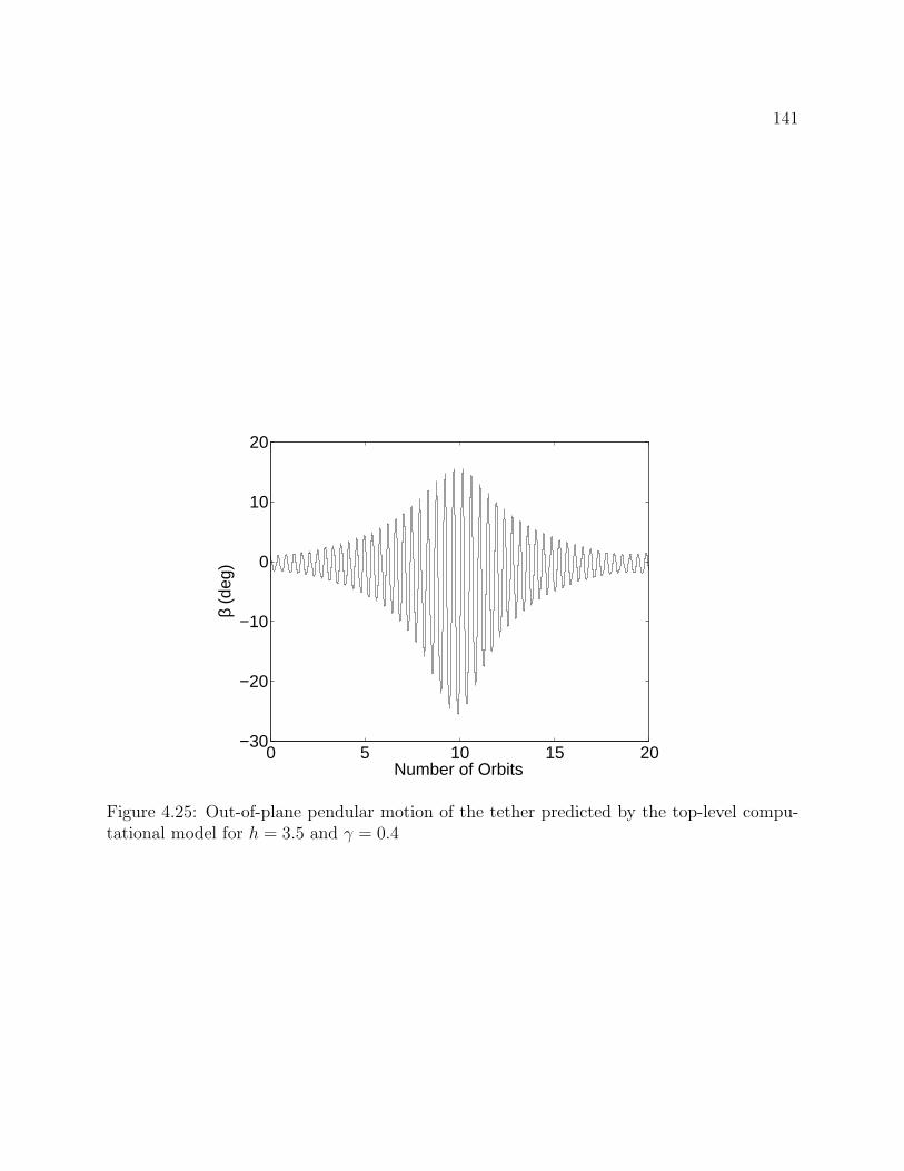
141

0 5 10 15 20−30

−20

−10

0

10

20

Number of Orbits

β (d

eg)

Figure 4.25: Out-of-plane pendular motion of the tether predicted by the top-level compu-tational model for h = 3.5 and γ = 0.4

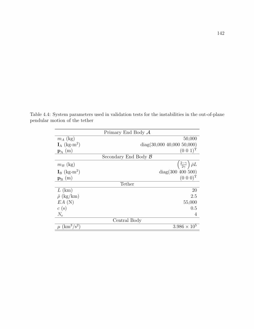
142

Table 4.4: System parameters used in validation tests for the instabilities in the out-of-planependular motion of the tether


Secondary End Body BmB (kg)

(2−γ2γ

)ρL

IB (kg-m2) diag(300 400 500)pB (m) (0 0 0)T



143

Table 4.5: Initial conditions used in validation tests for the instabilities in the out-of-planependular motion of the tether



ωA/O (deg/s) (0√hΩA0 0)T


ωB/O (deg/s) (0√hΩA0 0)T

Pendular Tether Motionα (deg) 0β (deg) 1

α (deg/s)√hΩA0


u(s, 0) (m) 20 sin(πsL

)u(s, 0) (m) 0v(s, 0) (m) 20 sin

(πsL

)v(s, 0) (m) 0

w(s, 0) (m) cALEA

f(0)[sL− γ

6

(sL

)3]

w(s, 0) (m) cALEA

f(0)[sL− γ

6

(sL

)3]

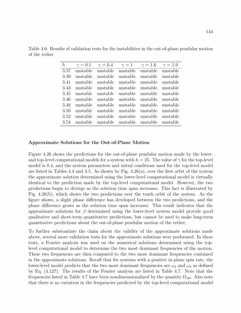
144

Table 4.6: Results of validation tests for the instabilities in the out-of-plane pendular motionof the tether

h γ = 0.1 γ = 0.4 γ = 1 γ = 1.6 γ = 1.93.37 unstable unstable unstable unstable unstable3.39 unstable unstable unstable unstable unstable3.41 unstable unstable unstable unstable unstable3.43 unstable unstable unstable unstable unstable3.45 unstable unstable unstable unstable unstable3.46 unstable unstable unstable unstable unstable3.48 unstable unstable unstable unstable unstable3.50 unstable unstable unstable unstable unstable3.52 unstable unstable unstable unstable unstable3.54 unstable unstable unstable unstable unstable

Approximate Solutions for the Out-of-Plane Motion

Figure 4.26 shows the predictions for the out-of-plane pendular motion made by the lower-and top-level computational models for a system with h = 25. The value of γ for the top-levelmodel is 0.4, and the system parameters and initial conditions used for the top-level modelare listed in Tables 4.4 and 4.5. As shown by Fig. 4.26(a), over the first orbit of the systemthe approximate solution determined using the lower-level computational model is virtuallyidentical to the prediction made by the top-level computational model. However, the twopredictions begin to diverge as the solution time span increases. This fact is illustrated byFig. 4.26(b), which shows the two predictions over the tenth orbit of the system. As thefigure shows, a slight phase difference has developed between the two predictions, and thephase difference grows as the solution time span increases. This result indicates that theapproximate solutions for β determined using the lower-level system model provide goodqualitative and short-term quantitative predictions, but cannot be used to make long-termquantitative predictions about the out-of-plane pendular motion of the tether.

To further substantiate the claim about the validity of the approximate solutions madeabove, several more validation tests for the approximate solutions were performed. In thesetests, a Fourier analysis was used on the numerical solutions determined using the top-level computational model to determine the two most dominant frequencies of the motion.These two frequencies are then compared to the two most dominant frequencies containedin the approximate solutions. Recall that for systems with a positive in-plane spin rate, thelower-level model predicts that the two most dominant frequencies are ω2 and ω3 as definedby Eq. (4.127). The results of the Fourier analysis are listed in Table 4.7. Note that thefrequencies listed in Table 4.7 have been nondimensionalized by the quantity ΩA0. Also notethat there is no variation in the frequencies predicted by the top-level computational model

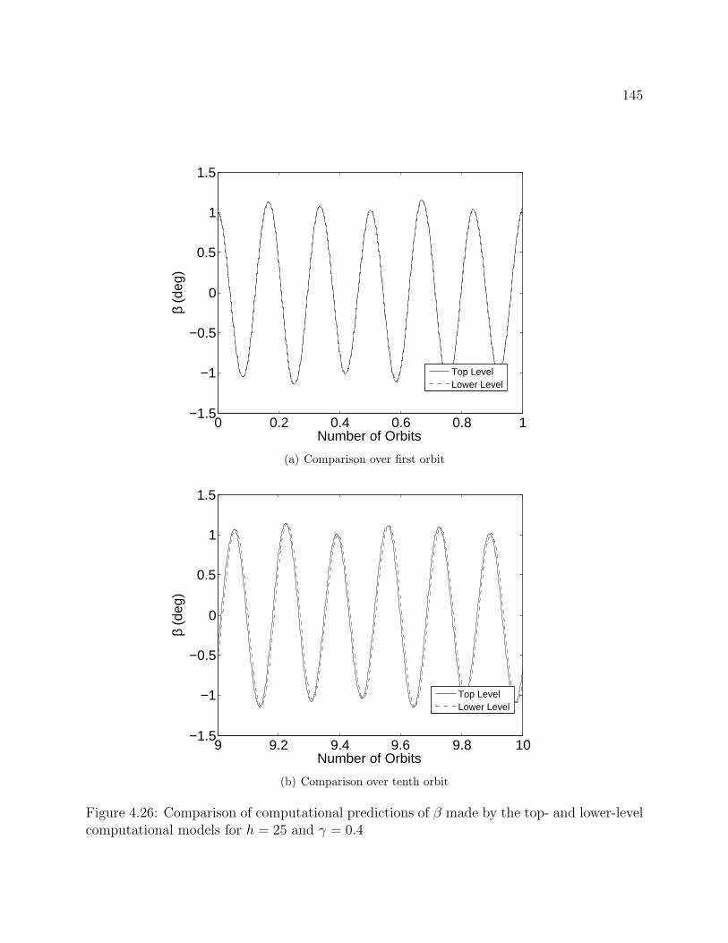
145

0 0.2 0.4 0.6 0.8 1−1.5

−1

−0.5

0

0.5

1

1.5

Number of Orbits

β (d

eg)

Top LevelLower Level

(a) Comparison over first orbit

9 9.2 9.4 9.6 9.8 10−1.5

−1

−0.5

0

0.5

1

1.5

Number of Orbits

β (d

eg)

Top LevelLower Level

(b) Comparison over tenth orbit

Figure 4.26: Comparison of computational predictions of β made by the top- and lower-levelcomputational models for h = 25 and γ = 0.4

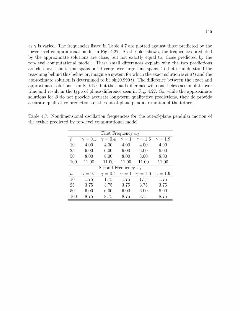
146

as γ is varied. The frequencies listed in Table 4.7 are plotted against those predicted by thelower-level computational model in Fig. 4.27. As the plot shows, the frequencies predictedby the approximate solutions are close, but not exactly equal to, those predicted by thetop-level computational model. These small differences explain why the two predictionsare close over short time spans but diverge over large time spans. To better understand thereasoning behind this behavior, imagine a system for which the exact solution is sin(t) and theapproximate solution is determined to be sin(0.999 t). The difference between the exact andapproximate solutions is only 0.1%, but the small difference will nonetheless accumulate overtime and result in the type of phase difference seen in Fig. 4.27. So, while the approximatesolutions for β do not provide accurate long-term qualitative predictions, they do provideaccurate qualitative predictions of the out-of-plane pendular motion of the tether.

Table 4.7: Nondimensional oscillation frequencies for the out-of-plane pendular motion ofthe tether predicted by top-level computational model

First Frequency ω2

h γ = 0.1 γ = 0.4 γ = 1 γ = 1.6 γ = 1.910 4.00 4.00 4.00 4.00 4.0025 6.00 6.00 6.00 6.00 6.0050 8.00 8.00 8.00 8.00 8.00100 11.00 11.00 11.00 11.00 11.00

Second Frequency ω3

h γ = 0.1 γ = 0.4 γ = 1 γ = 1.6 γ = 1.910 1.75 1.75 1.75 1.75 1.7525 3.75 3.75 3.75 3.75 3.7550 6.00 6.00 6.00 6.00 6.00100 8.75 8.75 8.75 8.75 8.75

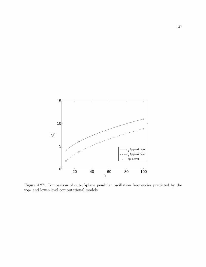
147

20 40 60 80 1000

5

10

15

h

|ωi|

ω2 Approximate

ω3 Approximate

Top−Level

Figure 4.27: Comparison of out-of-plane pendular oscillation frequencies predicted by thetop- and lower-level computational models

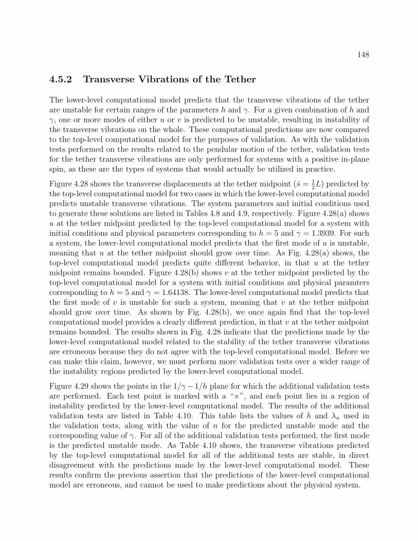
148

4.5.2 Transverse Vibrations of the Tether

The lower-level computational model predicts that the transverse vibrations of the tetherare unstable for certain ranges of the parameters h and γ. For a given combination of h andγ, one or more modes of either u or v is predicted to be unstable, resulting in instability ofthe transverse vibrations on the whole. These computational predictions are now comparedto the top-level computational model for the purposes of validation. As with the validationtests performed on the results related to the pendular motion of the tether, validation testsfor the tether transverse vibrations are only performed for systems with a positive in-planespin, as these are the types of systems that would actually be utilized in practice.

Figure 4.28 shows the transverse displacements at the tether midpoint (s = 12L) predicted by

the top-level computational model for two cases in which the lower-level computational modelpredicts unstable transverse vibrations. The system parameters and initial conditions usedto generate these solutions are listed in Tables 4.8 and 4.9, respectively. Figure 4.28(a) showsu at the tether midpoint predicted by the top-level computational model for a system withinitial conditions and physical parameters corresponding to h = 5 and γ = 1.3939. For sucha system, the lower-level computational model predicts that the first mode of u is unstable,meaning that u at the tether midpoint should grow over time. As Fig. 4.28(a) shows, thetop-level computational model predicts quite different behavior, in that u at the tethermidpoint remains bounded. Figure 4.28(b) shows v at the tether midpoint predicted by thetop-level computational model for a system with initial conditions and physical paramterscorresponding to h = 5 and γ = 1.64138. The lower-level computational model predicts thatthe first mode of v is unstable for such a system, meaning that v at the tether midpointshould grow over time. As shown by Fig. 4.28(b), we once again find that the top-levelcomputational model provides a clearly different prediction, in that v at the tether midpointremains bounded. The results shown in Fig. 4.28 indicate that the predictions made by thelower-level computational model related to the stability of the tether transverse vibrationsare erroneous because they do not agree with the top-level computational model. Before wecan make this claim, however, we must perform more validation tests over a wider range ofthe instability regions predicted by the lower-level computational model.

Figure 4.29 shows the points in the 1/γ− 1/h plane for which the additional validation testsare performed. Each test point is marked with a “×”, and each point lies in a region ofinstability predicted by the lower-level computational model. The results of the additionalvalidation tests are listed in Table 4.10. This table lists the values of h and λn used inthe validation tests, along with the value of n for the predicted unstable mode and thecorresponding value of γ. For all of the additional validation tests performed, the first modeis the predicted unstable mode. As Table 4.10 shows, the transverse vibrations predictedby the top-level computational model for all of the additional tests are stable, in directdisagreement with the predictions made by the lower-level computational model. Theseresults confirm the previous assertion that the predictions of the lower-level computationalmodel are erroneous, and cannot be used to make predictions about the physical system.

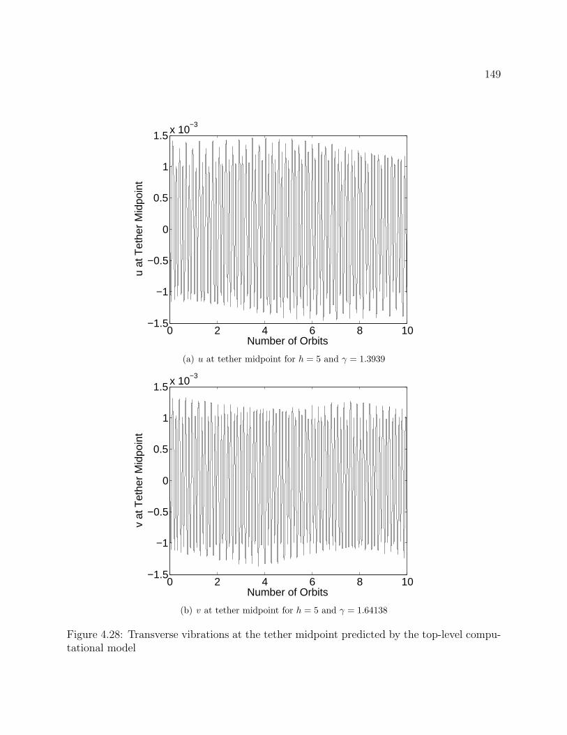
149

0 2 4 6 8 10−1.5

−1

−0.5

0

0.5

1

1.5 x 10−3

Number of Orbits

u at

Tet

her

Mid

poin

t

(a) u at tether midpoint for h = 5 and γ = 1.3939

0 2 4 6 8 10−1.5

−1

−0.5

0

0.5

1

1.5 x 10−3

Number of Orbits

v at

Tet

her

Mid

poin

t

(b) v at tether midpoint for h = 5 and γ = 1.64138

Figure 4.28: Transverse vibrations at the tether midpoint predicted by the top-level compu-tational model

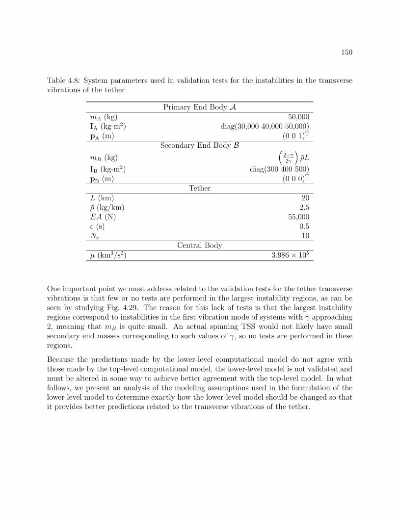
150

Table 4.8: System parameters used in validation tests for the instabilities in the transversevibrations of the tether


Secondary End Body BmB (kg)

(2−γ2γ

)ρL

IB (kg-m2) diag(300 400 500)pB (m) (0 0 0)T



One important point we must address related to the validation tests for the tether transversevibrations is that few or no tests are performed in the largest instability regions, as can beseen by studying Fig. 4.29. The reason for this lack of tests is that the largest instabilityregions correspond to instabilities in the first vibration mode of systems with γ approaching2, meaning that mB is quite small. An actual spinning TSS would not likely have smallsecondary end masses corresponding to such values of γ, so no tests are performed in theseregions.

Because the predictions made by the lower-level computational model do not agree withthose made by the top-level computational model, the lower-level model is not validated andmust be altered in some way to achieve better agreement with the top-level model. In whatfollows, we present an analysis of the modeling assumptions used in the formulation of thelower-level model to determine exactly how the lower-level model should be changed so thatit provides better predictions related to the transverse vibrations of the tether.

151

Table 4.9: Initial conditions used in validation tests for the instabilities in the transverse ofthe tether



ωA/O (deg/s) (0√hΩA0 0)T


ωB/O (deg/s) (0√hΩA0 0)T

Pendular Tether Motionα (deg) 0β (deg) 1

α (deg/s)√hΩA0



)u(s, 0) (m) 0v(s, 0) (m) 20 sin

(πsL

)v(s, 0) (m) 0

w(s, 0) (m) cALEA

f(0)[sL− γ

6

(sL

)3]

w(s, 0) (m) cALEA

f(0)[sL− γ

6

(sL

)3]

152

0 0.2 0.4 0.6 0.8 10

0.05

0.1

0.15

0.2

0.25

0.3

1/λ

1/h

(a) Validation tests for u

0 0.2 0.4 0.6 0.8 10

0.05

0.1

0.15

0.2

0.25

0.3

1/λ

1/h

(b) Validation tests for v

Figure 4.29: Points in the 1/γ − 1/h plane used for validation tests for the transversevibrations of the tether

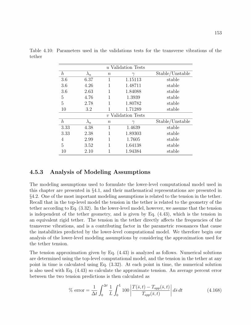
153

Table 4.10: Parameters used in the validations tests for the transverse vibrations of thetether

u Validation Testsh λn n γ Stable/Unstable3.6 6.37 1 1.15113 stable3.6 4.26 1 1.48711 stable3.6 2.63 1 1.84088 stable5 4.76 1 1.3939 stable5 2.78 1 1.80782 stable10 3.2 1 1.71289 stable

v Validation Testsh λn n γ Stable/Unstable3.33 4.38 1 1.4639 stable3.33 2.38 1 1.89303 stable4 2.99 1 1.7605 stable5 3.52 1 1.64138 stable10 2.10 1 1.94384 stable

4.5.3 Analysis of Modeling Assumptions

The modeling assumptions used to formulate the lower-level computational model used inthis chapter are presented in §4.1, and their mathematical representations are presented in§4.2. One of the most important modeling assumptions is related to the tension in the tether.Recall that in the top-level model the tension in the tether is related to the geometry of thetether according to Eq. (3.32). In the lower-level model, however, we assume that the tensionis independent of the tether geometry, and is given by Eq. (4.43), which is the tension inan equivalent rigid tether. The tension in the tether directly affects the frequencies of thetransverse vibrations, and is a contributing factor in the parametric resonances that causethe instabilities predicted by the lower-level computational model. We therefore begin ouranalysis of the lower-level modeling assumptions by considering the approximation used forthe tether tension.

The tension approximation given by Eq. (4.43) is analyzed as follows. Numerical solutionsare determined using the top-level computational model, and the tension in the tether at anypoint in time is calculated using Eq. (3.32). At each point in time, the numerical solutionis also used with Eq. (4.43) so calculate the approximate tension. An average percent errorbetween the two tension predictions is then calculated as

% error =1

∆t

∫ ∆t

0

1

L

∫ L

0

100

∣∣∣∣T (s, t)− Tapp(s, t)Tapp(s, t)

∣∣∣∣ ds dt (4.168)

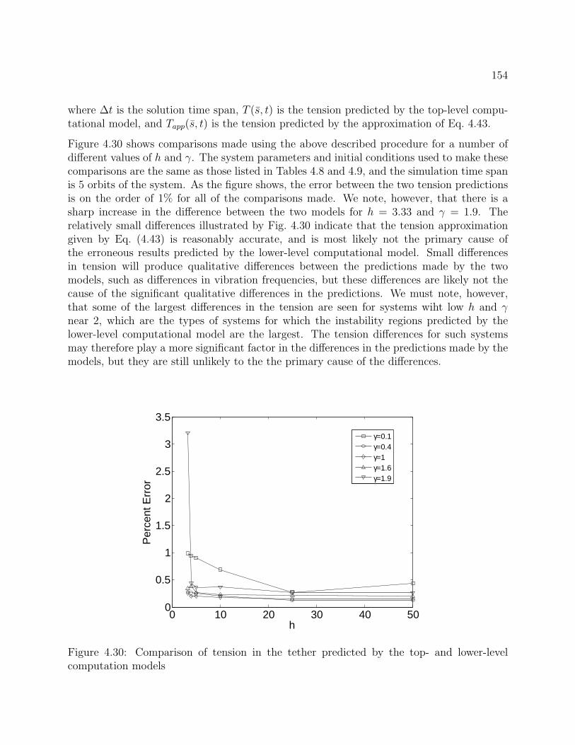
154

where ∆t is the solution time span, T (s, t) is the tension predicted by the top-level compu-tational model, and Tapp(s, t) is the tension predicted by the approximation of Eq. 4.43.

Figure 4.30 shows comparisons made using the above described procedure for a number ofdifferent values of h and γ. The system parameters and initial conditions used to make thesecomparisons are the same as those listed in Tables 4.8 and 4.9, and the simulation time spanis 5 orbits of the system. As the figure shows, the error between the two tension predictionsis on the order of 1% for all of the comparisons made. We note, however, that there is asharp increase in the difference between the two models for h = 3.33 and γ = 1.9. Therelatively small differences illustrated by Fig. 4.30 indicate that the tension approximationgiven by Eq. (4.43) is reasonably accurate, and is most likely not the primary cause ofthe erroneous results predicted by the lower-level computational model. Small differencesin tension will produce qualitative differences between the predictions made by the twomodels, such as differences in vibration frequencies, but these differences are likely not thecause of the significant qualitative differences in the predictions. We must note, however,that some of the largest differences in the tension are seen for systems wiht low h and γnear 2, which are the types of systems for which the instability regions predicted by thelower-level computational model are the largest. The tension differences for such systemsmay therefore play a more significant factor in the differences in the predictions made by themodels, but they are still unlikely to the the primary cause of the differences.

0 10 20 30 40 500

0.5

1

1.5

2

2.5

3

3.5

h

Per

cent

Err

or

γ=0.1γ=0.4γ=1γ=1.6γ=1.9

Figure 4.30: Comparison of tension in the tether predicted by the top- and lower-levelcomputation models

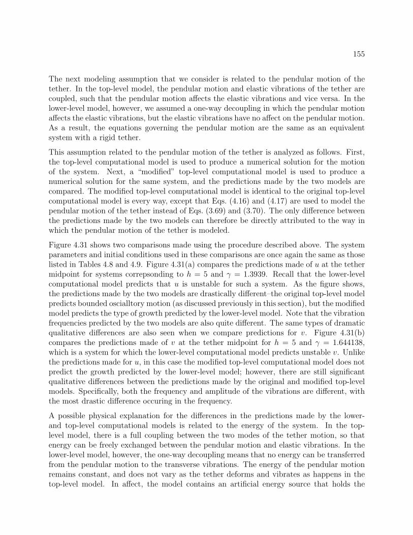
155

The next modeling assumption that we consider is related to the pendular motion of thetether. In the top-level model, the pendular motion and elastic vibrations of the tether arecoupled, such that the pendular motion affects the elastic vibrations and vice versa. In thelower-level model, however, we assumed a one-way decoupling in which the pendular motionaffects the elastic vibrations, but the elastic vibrations have no affect on the pendular motion.As a result, the equations governing the pendular motion are the same as an equivalentsystem with a rigid tether.

This assumption related to the pendular motion of the tether is analyzed as follows. First,the top-level computational model is used to produce a numerical solution for the motionof the system. Next, a “modified” top-level computational model is used to produce anumerical solution for the same system, and the predictions made by the two models arecompared. The modified top-level computational model is identical to the original top-levelcomputational model is every way, except that Eqs. (4.16) and (4.17) are used to model thependular motion of the tether instead of Eqs. (3.69) and (3.70). The only difference betweenthe predictions made by the two models can therefore be directly attributed to the way inwhich the pendular motion of the tether is modeled.

Figure 4.31 shows two comparisons made using the procedure described above. The systemparameters and initial conditions used in these comparisons are once again the same as thoselisted in Tables 4.8 and 4.9. Figure 4.31(a) compares the predictions made of u at the tethermidpoint for systems correpsonding to h = 5 and γ = 1.3939. Recall that the lower-levelcomputational model predicts that u is unstable for such a system. As the figure shows,the predictions made by the two models are drastically different–the original top-level modelpredicts bounded oscialltory motion (as discussed previously in this section), but the modifiedmodel predicts the type of growth predicted by the lower-level model. Note that the vibrationfrequencies predicted by the two models are also quite different. The same types of dramaticqualitative differences are also seen when we compare predictions for v. Figure 4.31(b)compares the predictions made of v at the tether midpoint for h = 5 and γ = 1.644138,which is a system for which the lower-level computational model predicts unstable v. Unlikethe predictions made for u, in this case the modified top-level computational model does notpredict the growth predicted by the lower-level model; however, there are still significantqualitative differences between the predictions made by the original and modified top-levelmodels. Specifically, both the frequency and amplitude of the vibrations are different, withthe most drastic difference occuring in the frequency.

A possible physical explanation for the differences in the predictions made by the lower-and top-level computational models is related to the energy of the system. In the top-level model, there is a full coupling between the two modes of the tether motion, so thatenergy can be freely exchanged between the pendular motion and elastic vibrations. In thelower-level model, however, the one-way decoupling means that no energy can be transferredfrom the pendular motion to the transverse vibrations. The energy of the pendular motionremains constant, and does not vary as the tether deforms and vibrates as happens in thetop-level model. In affect, the model contains an artificial energy source that holds the

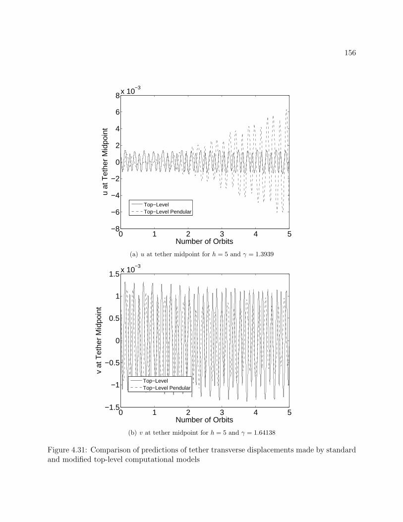
156

0 1 2 3 4 5−8

−6

−4

−2

0

2

4

6

8x 10−3

Number of Orbits

u at

Tet

her

Mid

poin

t

Top−LevelTop−Level Pendular

(a) u at tether midpoint for h = 5 and γ = 1.3939

0 1 2 3 4 5−1.5

−1

−0.5

0

0.5

1

1.5 x 10−3

Number of Orbits

v at

Tet

her

Mid

poin

t

Top−LevelTop−Level Pendular

(b) v at tether midpoint for h = 5 and γ = 1.64138

Figure 4.31: Comparison of predictions of tether transverse displacements made by standardand modified top-level computational models

157

energy of the pendular motion at a constant level. Because the pendular motion drives thetransverse vibrations, this artificial energy source in the pendular motion could certainlyhave a significant impact on the stability properties of the transverse vibrations.

Whatever their cause, the significant qualitative differences illustrated by Fig. 4.31 indicatethat modeling the pendular motion of the tether using Eqs. (4.16) and (4.17) has a significantaffect on the predictions of the tether transverse vibrations. It is quite unlikely that twocomputational models that demonstrate the qualitative differences seen in Fig. 4.31 will havethe same stability properties, so we conclude that the way in which the pendular motionis modeled is one of the, if not the, most significant factors contributing to the erroneouspredictions made by the lower-level computational model. Any future study of the tethertransverse vibrations made using a lower-level model must take into account the full couplingbetween the pendular motion and transverse vibrations of the tether.

Several other modeling assumptions may also contribute to the significant differences be-tween the predictions made by the top- and lower-level computational models. First, theeffects of the longitudinal vibrations of the tether may lead to significant differences betweenthe models–recall that the longitudinal vibrations are neglected in the lower-level model.Previous studies of axially extensible tethers have shown that the longitudinal vibrations arecoupled to the in-plane pendular motion of the tether,12,16 which in turn drives the transversevibrations. Considering the effects of the longitudinal vibrations may therefore be necessaryto accurately predict the stability properties of the transverse vibrations. Other modelingassumptions that may contribute tot he differences between the two models are constrainingthe system to an unperturbed circular orbit, modeling the end bodies as point masses, andassuming that gravity varies linearly over the length of the tether. For typical TSS, however,the differences in the predictions caused by these assumptions are most likely insignificantcompared to the differences caused by the assumptions discussed previously.

4.6 Summary

In this chapter we used a lower-level computational model to make predictions related tothe pendular motion and transverse elastic vibrations of the tether in a spinning TSS. Thelower-level model is a simplification of the top-level model that is intended to isolate thedynamics of the tether, which are assumed to be the only relevant dynamics in the system.

The equations governing the pendular motion of the tether in the lower-level model are thesame as those of an equivalent system in which the tether is rigid. These equations werelinearized about a nominal planar spinning motion and an exact analytical solution for thein-plane motion was determined in terms of Jacobi elliptic functions. Using the solution forthe in-plane motion in the linearized equation for the out-of-plane pendular motion resultsin a Hill’s equations, the stability properties of which were analyzed using Floquet theory.For certain in-plane spin rates the out-of-plane pendular motion was found to be unstable,

158

in that a small initial out-of-plane deviation grows large over time. The unstable growthis not necessarily unbounded, however, and the conservative nature of the system was usedto place bounds on the out-of-plane motion. For relatively high in-plane spin rates theout-of-plane pendular motion is stable, and approximate solutions were derived that arelinear combinations of four simple harmonic oscillators. Note that the results related to thestability of the out-of-plane motion and the approximate solutions for high in-plane spinrates are original contributions of this work.

The equations governing the transverse elastic vibrations of the tether in the lower-levelmodel are partial differential equations with time and arclength along the tether as inde-pendent variables. As done in the analysis of the pendular motion, these equations werelinearized about a nominal planar spinning motion, resulting in decoupled, linear, partialdifferential equations. The method of separation of variables was applied to these equations,and the mode shapes for the transverse vibrations were determined in terms of a hypergeo-metric function. The eigenvalues for the vibration modes and the solution for the in-planependular motion were then used in the equations governing the temporal components ofthe solutions for the transverse vibrations, resulting in Hill’s equations. Floquet theory wasused to show that the transverse vibrations are unstable for certain combinations of in-planespin rate and system mass distribution, with the largest instability regions corresponding tosystems with low in-plane spin rates and low secondary end mass relative to the tether mass.Note that these results related to the stability of the transverse vibrations duplicate thosepresented in Refs. [5] and [8].

The computational model validation procedure presented in Ch. 2 was applied to the predic-tions made by the lower-level computational model related to the pendular motion and elasticvibrations of the tether. The instabilities in the out-of-plane pendular motion predicted bythe lower-level model were also predicted by the top-level model for a wide range of systemparameters. These results are therefore considered validated, and we can expect a spinningTSS to experience unstable out-of-plane pendular motion for certain ranges of in-plane spinrate. The approximate solution for the out-of-plane pendular motion for high in-plane spinrates also compares favorably to predictions made by the top-level computational model. Theapproximate solutions accurately capture the qualitative characteristics of the out-of-planependular motion, and also provide accurate short-term quantitative predictions. However,the approximate solutions become less quantitatively accurate over expanding time scales,and should not be used for long-term quantitative predictions.

Unlike the predictions made by the lower-level computational model related to the pendularmotion of the tether, the predictions of unstable transverse vibrations were not predicted bythe top-level computational model. A number of validation tests were performed for severalsystems predicted to experience unstable transverse vibrations, and in all cases the top-levelcomputational model predicted that the transverse vibrations remain bounded. The lower-level computational model is therefore not validated in this case, and must be altered in someway to achieve better agreement with the top-level computational model. An analysis of themodeling assumptions used to formulate the lower-level model showed that the assumption

159

of a one-way coupling between the pendular motion and transverse vibrations is the mostlikely cause of the erroneous predictions. Any further study of the transverse vibrations ofthe tether must therefore relax this assumption.

The results of the validation tests on the predictions of instability in the tether transverse vi-brations clearly demonstrate the necessity of performing some form of validation on resultsobtained from lower-level computational models. These results are undoubedtly mathe-matically correct, and, as mentioned several times in this dissertation, have been reportedpreviously in the literature. The mathematical correctness of a prediction, however, doesnot guarantee that it can be applied to the particular physical system of interest, as demon-strated by the work presented in this chapter. The applicability of a prediction made by alower-level computational model can only be determined by validating it against data that isbelieved to sufficiently represent the behavior of the actual physical system. In the absenceof experimental data, we believe that the validation procedure presented in Ch. 2 and appliedin this chapter is the best available option.

Chapter 5

Control of Spinning Tethered SatelliteSystems

In Ch. 4 we presented a detailed analysis of the motion of the tether in a spinning TSS. Alower-level computational model was used to analyze both the pendular motion and trans-verse elastic vibrations of the tether, and the computational model validation procedureoutlined in Ch. 2 was used to validate the predictions pertaining to the pendular motion.The dynamic analysis of the pendular motion presented in Ch. 4 is fairly complete, so thenatural next step in the analysis of the pendular motion is to develop methods of controllingsuch motion.

In this chapter we considered numerous methods of controlling the pendular motion of thetether in a spinning TSS. Because the nominal motion of a spinning TSS is in the orbit plane,all of the control developments drive the tether to a planar pendular motion. We begin thecontrol developments by considering the possibility of controlling the pendular motion usingelectrodynamic thrusting as the only control actuator. A nonlinear controllability analysisis used to show that such control is not possible, and other means of control actuation mustbe employed. Several different nonlinear control design techniques are then used to developcontrol laws that drive the system to a desired planar motion. All of these control laws aredeveloped using a lower-level computational model, so they are also applied to the top-levelcomputational model to assess their applicability and effectiveness.


The physical system and conceptual model considered in the control analysis are the sameas those used in the dynamic analysis presented in Ch. 4. See §4.1 for a complete descriptionof these elements of the system model. One of the key assumptions utilized in the controldevelopments that follow is that the elastic vibrations of the tether have no effect on the

160

161

pendular motion of the tether. This assumption allows us to use a greatly simplified math-ematical model of the pendular motion to develop control laws. One final element of theconceptual model we must consider that is not discussed in §4.1 is related to the magneticfield of the central body: because we consider the possibility of controlling the pendular mo-tion using electrodynamic thrusting, we must have a conceptual model of the magnetic fieldof the central body. As done for the top-level system model, we assume that the magneticfield is a tilted dipole that is fixed to the central body as it rotates.


Because the conceptual model used in the control analysis is the same as that used in Ch. 4,the mathematical model used in this chapter is virtually identical to the one derived inSec. 4.2. However, we only need to consider the equations governing the pendular motion ofthe tether (which are not affected by the transverse elastic vibrations of the tether), and wemust modify the pendular equations of motion to include methods of control actuation.

As shown in §4.2.3, the equations of motion governing the pendular motion of the tether canbe expressed as in Eq. (4.11). In §4.2.3, the external moment acting on the system about A,~MA, is due to the gravity-gradient moment only. We must now modify ~MA to include theeffects of electrodynamic forcing and other methods of control actuation.

The moment about A due to the electrodynamic force can be expressed as

~MEA =

∫ L

0

~r× (i d~r× ~B) (5.1)

where i is the current in the tether and ~B is the magnetic field vector. Assuming thatthe elastic vibrations of the tether have a negligible influence on the total electrodynamicmoment, we make the approximations

~r ≈ se3 (5.2)

d~r ≈ dse3 (5.3)

such that Eq. (5.1) becomes

~MEA =

∫ L

0

se3 × (i dse3 × ~B) (5.4)

Expressing ~B relative to FE as

~B = B1e1 +B2e2 +B3e3 (5.5)

we have

~MEA = −i(∫ L

0

sB1 ds

)e1 − i

(∫ L

0

sB2 ds

)e2 (5.6)

162

Note that we have assumed that i is constant along the length of the tether, as done in thetop-level model.

Letting the moment about A due to any other external forces be

~MAF = MAF1e1 +MAF2e2 (5.7)

(there can be no moment about the e3 axis because the system has no dimension about thataxis) and making use of the gravity-gradient moment expression defined in Eq. (4.15), thetotal external moment acting on the system about A can be written as

~MA = MA1e1 +MA2e2 (5.8)

where

MA1 = 3IAΩ2A cos2 α sin β cos β − i

(∫ L

0

sB1 ds

)+MAF1 (5.9)

MA2 = −3IAΩ2A sinα cosα cos β − i

(∫ L

0

sB2 ds

)+MAF2 (5.10)

Using Eqs. (5.9) and (5.10) in Eq. (4.11), the equations of motion governing the pendularmotion of the tether are

α cos β − 2(α + ΩA)β sin β + 3Ω2A sinα cosα cos β = − i

IA

(∫ L

0

sB2 ds

)+MAF2

IA(5.11)

β + [(α + ΩA)2 + 3Ω2A cos2 α] sin β cos β =

i

IA

(∫ L

0

sB2 ds

)− MAF1

IA(5.12)

Making use of several of the nondimensional quantities defined in §4.2.5, Eqs. (5.11) and(5.12) are cast in nondimensional form as

α cos β − 2(

α + 1)

β sin β + 3 sinα cosα cos β = −ε

∫ 1

0

2xb2 dx+ uα (5.13)

β + [(

α + 1)2 + 3 cos2 α] sin β cos β = ε

∫ 1

0

2xb1 dx+ uβ (5.14)

where we have defined the quantities

ε =iL2

2IA

(µMµ

)(5.15)

bi =

(r3A

µM

)Bi (5.16)

uα =MAF2

IAΩ2A

(5.17)

uβ = −MAF1

IAΩ2A

(5.18)

163

Note that µM is the strength of the magnetic dipole of the central body.

Equations (5.13) and (5.14) are the equations used in the remainder of this chapter to developmethods of controlling the pendular motion of the tether. The control inputs are taken tobe ε, which is related to the electrodynamic force acting on the tether, and uα and uβ, whichare related to any non-electrodynamic moments acting on the system. Modulation of ε canbe achieved by changing the current in the tether, possibly by means of a variable resistoror on-board voltage source. The physical source of the inputs uα and uβ is assumed to bearbitrary at this point; however, we do note that these inputs would most likely be providedby small thrusters on the secondary end body.

5.3 Computational Model: Control of Pendular Mo-

tion

In this section we use Eqs. (5.13) and (5.14) along with various nonlinear control designtechniques to develop methods of controlling the pendular motion of the tether. Becausethe nominal pendular motion of a spinning TSS is in the orbit plane, we desire control

laws that drive β andβ to zero while driving the in-plane pendular motion to a desired

reference trajectory. We begin the control analysis by studying the feasibility of performingsuch control maneuvers using the electrodynamic force as the only control actuator. Thisanalysis serves to motivate the control law developments presented later in this section.

5.3.1 Controllability Using Electrodynamic Forcing

If the electrodynamic force is allowed to be the only control input, the equations of motiongoverning the pendular motion of the tether become

α cos β − 2(

α + 1)

β sin β + 3 sinα cosα cos β = −ε

∫ 1

0

2xb2 dx (5.19)

β + [(

α + 1)2 + 3 cos2 α] sin β cos β = ε

∫ 1

0

2xb1 dx (5.20)

At this point we make several assumptions related to the magnetic field of the central bodydesigned to simplify the electrodynamic moment expressions in Eqs. (5.19) and (5.20). Theobjective of the current analysis is to demonstrate the inherent difficulties in controlling thependular motion of the tether using electrodynamic forcing only, and the conclusions of thisanalysis are valid for general magnetic field models. We therefore use the simplest possiblerepresentation of the magnetic field: a nontilted, nonrotating dipole. We further assumethat the circular orbit of A is constrained to the plane of the magnetic equator. Under

164

these assumptions, the unit dipole axis is aligned with the orbit normal direction, and themagnetic field vector at any point along the tether is

~B =µMr3T

o2

=µMr3T

(cos βe2 + sin βe3)(5.21)

where rT is the orbital radius of a differential tether element, ds. Because the length of thetether in a typical TSS is much smaller than the orbit radius of the system, we linearizeEq. (5.21) about the position of A to obtain

~B =µMr3A

(1− 3`x cosα cos β)(cos βe2 + sin βe3) (5.22)

where we have defined the nondimensional parameter

` =L

rA(5.23)

From Eq. (5.16), we have b1 = 0 and

b2 = (1− 3`x cosα cos β) cos β (5.24)

Using these quantities in Eqs. (5.19) and (5.20), the equations governing the pendular motionof the tether become

α cos β − 2(

α + 1)

β sin β + 3 sinα cosα cos β = −ε(1− 2` cosα cos β) cos β (5.25)

β + [(

α + 1)2 + 3 cos2 α] sin β cos β = 0 (5.26)

The controllability analysis of Eqs. (5.25) and (5.26) requires that they be in state-spaceform. Define the state vector

x =(α β

α

β)T

(5.27)

the control input u = ε, and the quantities

f(x) =

αβ

2(α + 1)

β tan β − 3 sinα cosα

−[(α + 1)2 + 3 cos2 α] sin β cos β

(5.28)

g(x) =

00

2` cosα cos β − 10

(5.29)

165

Using these definitions, Eqs. (5.25) and (5.26) are rewritten as

x = f(x) + g(x)u (5.30)

Equation (5.30) is the standard form for a single-input nonlinear control system.

According the nonlinear control theory,28,42,58 the system defined by Eqs. (5.28–5.30) isaccessible in a region D ⊆ <4 of the state-space if the matrix

C =[

g [f,g] [f, [f,g]] [f, [f, [f,g]]]]

(5.31)

is full-rank at every point in D, where the Lie bracket [a,b] is defined as

[a,b] =∂b

∂xa− ∂a

∂xb (5.32)

(See Corollary 3.11 of Ref. [42].) Another way of stating this accessibility condition is thatthe determinant of C must be nonzero at every point in D. Using Eqs. (5.28) and (5.29) inEq. (5.31) to form C and taking its determinant, we obtain

|C| = −(1− 2` cosα cos β)4(α + 1)2

[(5 + 3 cos(2α) + 2

α(α + 2)) sin2(2β) + 8

β2]

cos2 β

(5.33)From Eq. (5.33), we can see that there are a number of states that result in the determinantof C becoming 0, meaning that the system is not accessible. Because the system is notaccessible, it is also not controllable. Most notably, any motion in the α −

α plane (corre-

sponding to β =β = 0) is not accessible. This makes sense physically, because motion in

the α− α plane results in an electrodynamic force in the α−

α plane as well, and β cannotbe controlled.

The above analysis illustrates the inherent difficulty of controlling the pendular motion of thetether using only the electrodynamic force: the nature of the electrodynamic force constrainsit to be in a specific direction, perpindicular to both the tether and the magnetic field vector,at any point in time. The lack of control over the direction of the force is the factor thatleads to the difficulty in controlling α and β simultaneously.

Upon further inspection, it may seem that there really is no difficultly in using the electro-dynamic force to control the pendular motion of a spinning TSS because, for such a system,we want to control the motion to the α −

α plane, after which point we do not need anycontrol authority over β. However, this appearance of controllability is simply an artifact ofthe simplified magnetic field model used in the analysis presented above. If a more realisticmagnetic field model is used (such as the tilted, rotating dipole model used in the top-levelsystem model), in general there is always a component of the electrodynamic force out ofthe orbit plane, and it is not possible to drive to motion to the orbit plane and then controlthe in-plane motion as desired. The subsequent control of the in-plane motion necessarilyresults in out-of-plane pendular motion, which would then have to be controlled back to zerosomehow.

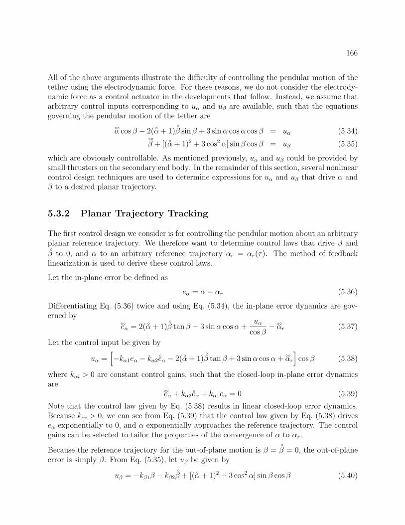
166

All of the above arguments illustrate the difficulty of controlling the pendular motion of thetether using the electrodynamic force. For these reasons, we do not consider the electrody-namic force as a control actuator in the developments that follow. Instead, we assume thatarbitrary control inputs corresponding to uα and uβ are available, such that the equationsgoverning the pendular motion of the tether are

α cos β − 2(

α + 1)

β sin β + 3 sinα cosα cos β = uα (5.34)

β + [(

α + 1)2 + 3 cos2 α] sin β cos β = uβ (5.35)

which are obviously controllable. As mentioned previously, uα and uβ could be provided bysmall thrusters on the secondary end body. In the remainder of this section, several nonlinearcontrol design techniques are used to determine expressions for uα and uβ that drive α andβ to a desired planar trajectory.

5.3.2 Planar Trajectory Tracking

The first control design we consider is for controlling the pendular motion about an arbitraryplanar reference trajectory. We therefore want to determine control laws that drive β andβ to 0, and α to an arbitrary reference trajectory αr = αr(τ). The method of feedbacklinearization is used to derive these control laws.

Let the in-plane error be defined as

eα = α− αr (5.36)

Differentiating Eq. (5.36) twice and using Eq. (5.34), the in-plane error dynamics are gov-erned by

eα = 2(

α + 1)

β tan β − 3 sinα cosα +

uαcos β

− αr (5.37)

Let the control input be given by

uα =[−kα1eα − kα2

eα − 2(

α + 1)

β tan β + 3 sinα cosα +

αr

]cos β (5.38)

where kαi > 0 are constant control gains, such that the closed-loop in-plane error dynamicsare

eα + kα2

eα + kα1eα = 0 (5.39)

Note that the control law given by Eq. (5.38) results in linear closed-loop error dynamics.Because kαi > 0, we can see from Eq. (5.39) that the control law given by Eq. (5.38) driveseα exponentially to 0, and α exponentially approaches the reference trajectory. The controlgains can be selected to tailor the properties of the convergence of α to αr.

Because the reference trajectory for the out-of-plane motion is β =β = 0, the out-of-plane

error is simply β. From Eq. (5.35), let uβ be given by

uβ = −kβ1β − kβ2

β + [(

α + 1)2 + 3 cos2 α] sin β cos β (5.40)

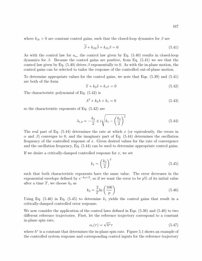
167

where kβi > 0 are constant control gains, such that the closed-loop dynamics for β are

β + kβ2

β + kβ1β = 0 (5.41)

As with the control law for uα, the control law given by Eq. (5.40) results in closed-loopdynamics for β. Because the control gains are positive, from Eq. (5.41) we see that thecontrol law given by Eq. (5.40) drives β exponentially to 0. As with the in-plane motion, thecontrol gains can be selected to tailor the response of the controlled out-of-plane motion.

To determine appropriate values for the control gains, we note that Eqs. (5.39) and (5.41)are both of the form

x+ k2

x+ k1x = 0 (5.42)

The characteristic polynomial of Eq. (5.42) is

λ2 + k2λ+ k1 = 0 (5.43)

so the characteristic exponents of Eq. (5.42) are

λ1,2 = −k2

2± i

√k1 −

(k2

2

)2

(5.44)

The real part of Eq. (5.44) determines the rate at which x (or equivalently, the errors inα and β) converges to 0, and the imaginary part of Eq. (5.44) determines the oscillationfrequency of the controlled response of x. Given desired values for the rate of convergenceand the oscillation frequency, Eq. (5.44) can be used to determine appropriate control gains.

If we desire a critically-damped controlled response for x, we set

k1 =

(k2

2

)2

(5.45)

such that both characteristic exponents have the same value. The error decreases in theexponential envelope defined by e−k2τ/2, so if we want the error to be p% of its initial valueafter a time T , we choose k2 as

k2 =2

Tln

(100

p

)(5.46)

Using Eq. (5.46) in Eq. (5.45) to determine k1 yields the control gains that result in acritically-damped controlled error response.

We now consider the application of the control laws defined in Eqs. (5.38) and (5.40) to twodifferent reference trajectories. First, let the reference trajectory correspond to a constantin-plane spin rate,

αr(τ) =√h∗τ (5.47)

where h∗ is a constant that determines the in-plane spin rate. Figure 5.1 shows an example ofthe controlled system response and corresponding control inputs for the reference trajectory

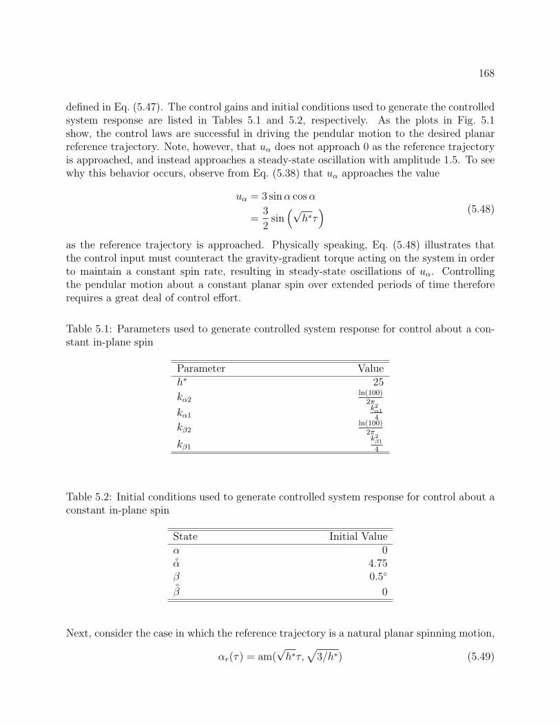
168

defined in Eq. (5.47). The control gains and initial conditions used to generate the controlledsystem response are listed in Tables 5.1 and 5.2, respectively. As the plots in Fig. 5.1show, the control laws are successful in driving the pendular motion to the desired planarreference trajectory. Note, however, that uα does not approach 0 as the reference trajectoryis approached, and instead approaches a steady-state oscillation with amplitude 1.5. To seewhy this behavior occurs, observe from Eq. (5.38) that uα approaches the value

uα = 3 sinα cosα

=3

2sin(√

h∗τ) (5.48)

as the reference trajectory is approached. Physically speaking, Eq. (5.48) illustrates thatthe control input must counteract the gravity-gradient torque acting on the system in orderto maintain a constant spin rate, resulting in steady-state oscillations of uα. Controllingthe pendular motion about a constant planar spin over extended periods of time thereforerequires a great deal of control effort.

Table 5.1: Parameters used to generate controlled system response for control about a con-stant in-plane spin

Parameter Valueh∗ 25

kα2ln(100)

2π

kα1k2α1

4

kβ2ln(100)

2π

kβ1k2β1

4

Table 5.2: Initial conditions used to generate controlled system response for control about aconstant in-plane spin

State Initial Valueα 0α 4.75β 0.5β 0

Next, consider the case in which the reference trajectory is a natural planar spinning motion,

αr(τ) = am(√h∗τ,

√3/h∗) (5.49)

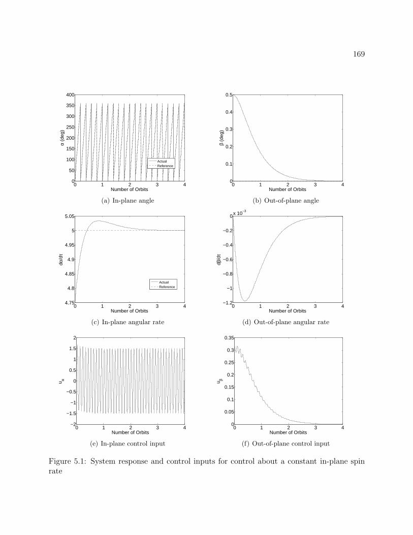
169

0 1 2 3 40

50

100

150

200

250

300

350

400

Number of Orbits

α (d

eg)

ActualReference

(a) In-plane angle

0 1 2 3 40

0.1

0.2

0.3

0.4

0.5

Number of Orbits

β (d

eg)

(b) Out-of-plane angle

0 1 2 3 44.75

4.8

4.85

4.9

4.95

5

5.05

Number of Orbits

dα/d

τ

ActualReference

(c) In-plane angular rate

0 1 2 3 4−1.2

−1

−0.8

−0.6

−0.4

−0.2

0x 10−3

Number of Orbits

dβ/d

τ

(d) Out-of-plane angular rate

0 1 2 3 4−2

−1.5

−1

−0.5

0

0.5

1

1.5

2

Number of Orbits

u α

(e) In-plane control input

0 1 2 3 40

0.05

0.1

0.15

0.2

0.25

0.3

0.35

Number of Orbits

u β

(f) Out-of-plane control input

Figure 5.1: System response and control inputs for control about a constant in-plane spinrate

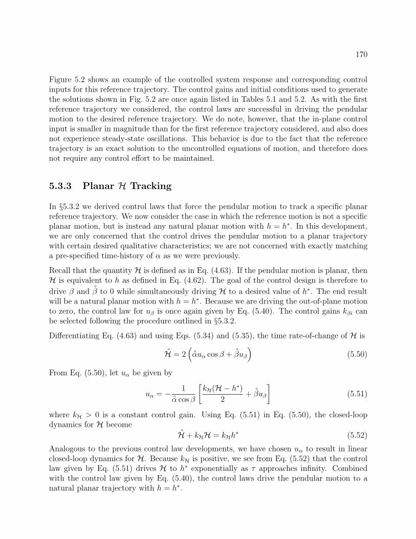
170

Figure 5.2 shows an example of the controlled system response and corresponding controlinputs for this reference trajectory. The control gains and initial conditions used to generatethe solutions shown in Fig. 5.2 are once again listed in Tables 5.1 and 5.2. As with the firstreference trajectory we considered, the control laws are successful in driving the pendularmotion to the desired reference trajectory. We do note, however, that the in-plane controlinput is smaller in magnitude than for the first reference trajectory considered, and also doesnot experience steady-state oscillations. This behavior is due to the fact that the referencetrajectory is an exact solution to the uncontrolled equations of motion, and therefore doesnot require any control effort to be maintained.

5.3.3 Planar H Tracking

In §5.3.2 we derived control laws that force the pendular motion to track a specific planarreference trajectory. We now consider the case in which the reference motion is not a specificplanar motion, but is instead any natural planar motion with h = h∗. In this development,we are only concerned that the control drives the pendular motion to a planar trajectorywith certain desired qualitative characteristics; we are not concerned with exactly matchinga pre-specified time-history of α as we were previously.

Recall that the quantity H is defined as in Eq. (4.63). If the pendular motion is planar, thenH is equivalent to h as defined in Eq. (4.62). The goal of the control design is therefore to

drive β andβ to 0 while simultaneously driving H to a desired value of h∗. The end result

will be a natural planar motion with h = h∗. Because we are driving the out-of-plane motionto zero, the control law for uβ is once again given by Eq. (5.40). The control gains kβi canbe selected following the procedure outlined in §5.3.2.

Differentiating Eq. (4.63) and using Eqs. (5.34) and (5.35), the time rate-of-change of H is

H = 2

(αuα cos β +

βuβ

)(5.50)

From Eq. (5.50), let uα be given by

uα = − 1α cos β

[kH(H− h∗)

2+βuβ

](5.51)

where kH > 0 is a constant control gain. Using Eq. (5.51) in Eq. (5.50), the closed-loopdynamics for H become

H + kHH = kHh

∗ (5.52)

Analogous to the previous control law developments, we have chosen uα to result in linearclosed-loop dynamics for H. Because kH is positive, we see from Eq. (5.52) that the controllaw given by Eq. (5.51) drives H to h∗ exponentially as τ approaches infinity. Combinedwith the control law given by Eq. (5.40), the control laws drive the pendular motion to anatural planar trajectory with h = h∗.

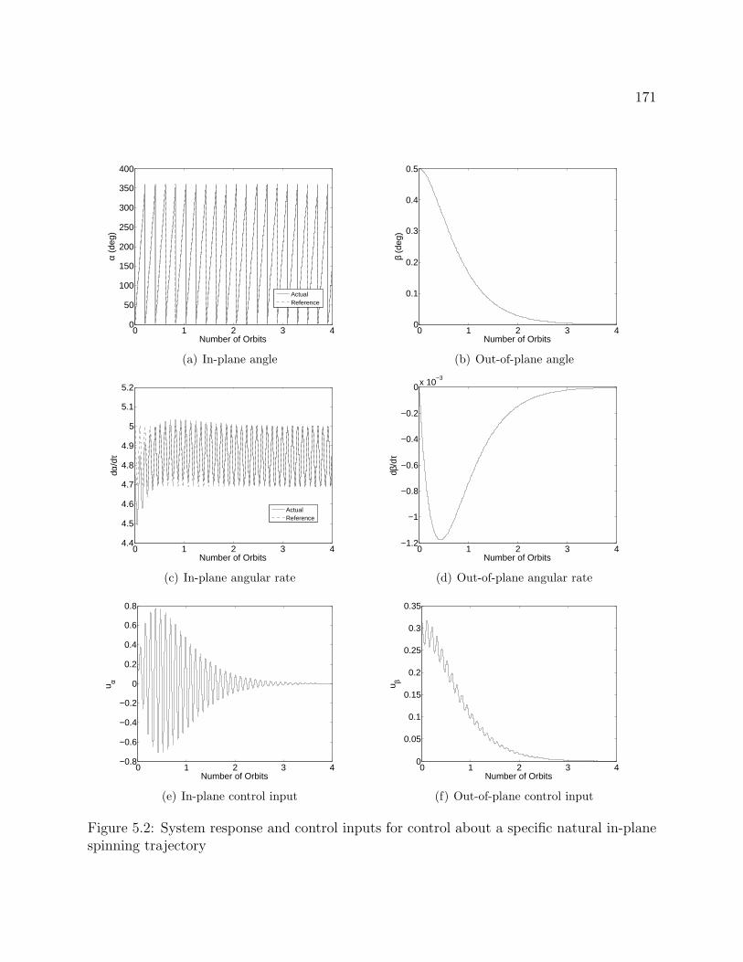
171

0 1 2 3 40

50

100

150

200

250

300

350

400

Number of Orbits

α (d

eg)

ActualReference

(a) In-plane angle

0 1 2 3 40

0.1

0.2

0.3

0.4

0.5

Number of Orbits

β (d

eg)


0 1 2 3 44.4

4.5

4.6

4.7

4.8

4.9

5

5.1

5.2

Number of Orbits

dα/d

τ

ActualReference


0 1 2 3 4−1.2

−1

−0.8

−0.6

−0.4

−0.2

0x 10−3

Number of Orbits

dβ/d

τ


0 1 2 3 4−0.8

−0.6

−0.4

−0.2

0

0.2

0.4

0.6

0.8

Number of Orbits

u α

(e) In-plane control input

0 1 2 3 40

0.05

0.1

0.15

0.2

0.25

0.3

0.35

Number of Orbits

u β

(f) Out-of-plane control input

Figure 5.2: System response and control inputs for control about a specific natural in-planespinning trajectory

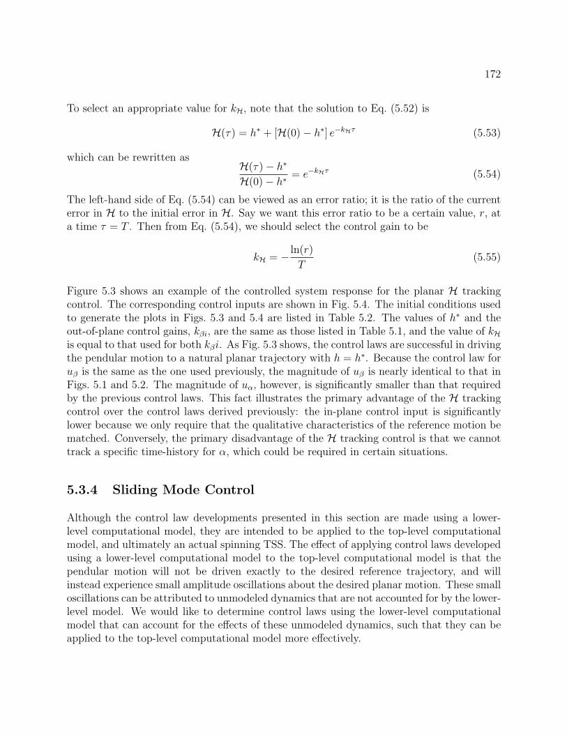
172

To select an appropriate value for kH, note that the solution to Eq. (5.52) is

H(τ) = h∗ + [H(0)− h∗] e−kHτ (5.53)

which can be rewritten asH(τ)− h∗

H(0)− h∗= e−kHτ (5.54)

The left-hand side of Eq. (5.54) can be viewed as an error ratio; it is the ratio of the currenterror in H to the initial error in H. Say we want this error ratio to be a certain value, r, ata time τ = T . Then from Eq. (5.54), we should select the control gain to be

kH = − ln(r)

T(5.55)

Figure 5.3 shows an example of the controlled system response for the planar H trackingcontrol. The corresponding control inputs are shown in Fig. 5.4. The initial conditions usedto generate the plots in Figs. 5.3 and 5.4 are listed in Table 5.2. The values of h∗ and theout-of-plane control gains, kβi, are the same as those listed in Table 5.1, and the value of kHis equal to that used for both kβi. As Fig. 5.3 shows, the control laws are successful in drivingthe pendular motion to a natural planar trajectory with h = h∗. Because the control law foruβ is the same as the one used previously, the magnitude of uβ is nearly identical to that inFigs. 5.1 and 5.2. The magnitude of uα, however, is significantly smaller than that requiredby the previous control laws. This fact illustrates the primary advantage of the H trackingcontrol over the control laws derived previously: the in-plane control input is significantlylower because we only require that the qualitative characteristics of the reference motion bematched. Conversely, the primary disadvantage of the H tracking control is that we cannottrack a specific time-history for α, which could be required in certain situations.

5.3.4 Sliding Mode Control

Although the control law developments presented in this section are made using a lower-level computational model, they are intended to be applied to the top-level computationalmodel, and ultimately an actual spinning TSS. The effect of applying control laws developedusing a lower-level computational model to the top-level computational model is that thependular motion will not be driven exactly to the desired reference trajectory, and willinstead experience small amplitude oscillations about the desired planar motion. These smalloscillations can be attributed to unmodeled dynamics that are not accounted for by the lower-level model. We would like to determine control laws using the lower-level computationalmodel that can account for the effects of these unmodeled dynamics, such that they can beapplied to the top-level computational model more effectively.

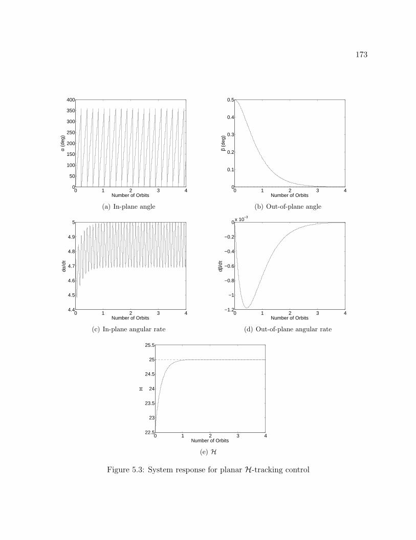
173

0 1 2 3 40

50

100

150

200

250

300

350

400

Number of Orbits

α (d

eg)

(a) In-plane angle

0 1 2 3 40

0.1

0.2

0.3

0.4

0.5

Number of Orbits

β (d

eg)


0 1 2 3 44.4

4.5

4.6

4.7

4.8

4.9

5

Number of Orbits

dα/d

τ


0 1 2 3 4−1.2

−1

−0.8

−0.6

−0.4

−0.2

0x 10−3

Number of Orbits

dβ/d

τ


0 1 2 3 422.5

23

23.5

24

24.5

25

25.5

Number of Orbits

H

(e) H

Figure 5.3: System response for planar H-tracking control

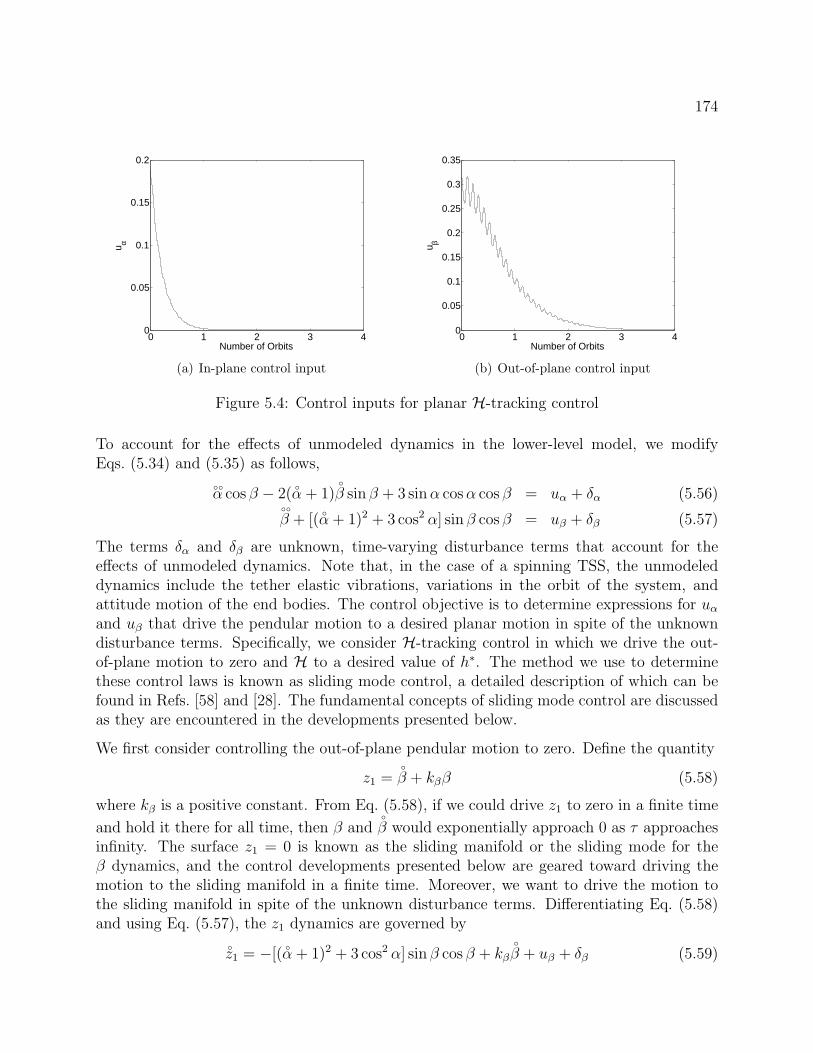
174

0 1 2 3 40

0.05

0.1

0.15

0.2

Number of Orbits

u α

(a) In-plane control input

0 1 2 3 40

0.05

0.1

0.15

0.2

0.25

0.3

0.35

Number of Orbits

u β

(b) Out-of-plane control input

Figure 5.4: Control inputs for planar H-tracking control

To account for the effects of unmodeled dynamics in the lower-level model, we modifyEqs. (5.34) and (5.35) as follows,

α cos β − 2(

α + 1)

β sin β + 3 sinα cosα cos β = uα + δα (5.56)

β + [(

α + 1)2 + 3 cos2 α] sin β cos β = uβ + δβ (5.57)

The terms δα and δβ are unknown, time-varying disturbance terms that account for theeffects of unmodeled dynamics. Note that, in the case of a spinning TSS, the unmodeleddynamics include the tether elastic vibrations, variations in the orbit of the system, andattitude motion of the end bodies. The control objective is to determine expressions for uαand uβ that drive the pendular motion to a desired planar motion in spite of the unknowndisturbance terms. Specifically, we consider H-tracking control in which we drive the out-of-plane motion to zero and H to a desired value of h∗. The method we use to determinethese control laws is known as sliding mode control, a detailed description of which can befound in Refs. [58] and [28]. The fundamental concepts of sliding mode control are discussedas they are encountered in the developments presented below.

We first consider controlling the out-of-plane pendular motion to zero. Define the quantity

z1 =β + kββ (5.58)

where kβ is a positive constant. From Eq. (5.58), if we could drive z1 to zero in a finite time

and hold it there for all time, then β andβ would exponentially approach 0 as τ approaches

infinity. The surface z1 = 0 is known as the sliding manifold or the sliding mode for theβ dynamics, and the control developments presented below are geared toward driving themotion to the sliding manifold in a finite time. Moreover, we want to drive the motion tothe sliding manifold in spite of the unknown disturbance terms. Differentiating Eq. (5.58)and using Eq. (5.57), the z1 dynamics are governed by

z1 = −[(

α + 1)2 + 3 cos2 α] sin β cos β + kβ

β + uβ + δβ (5.59)

175

From Eq. (5.59), let the control input be

uβ = [(α + 1)2 + 3 cos2 α] sin β cos β − kβ

β + vβ (5.60)

such that Eq. (5.59) becomesz1 = vβ + δβ (5.61)

Note that we have chosen uβ to cancel the known, nonlinear components of Eq. (5.59) whileleaving the unknown disturbance term. The term vβ must now be chosen to account for δβ.

Define the candidate Lyapunov function for the z1 dynamics as

V1 =1

2z2

1 (5.62)

which is positive definite about z1 = 0. Differentiating Eq. (5.62) and using Eq. (5.61), therate-of-change of V1 along the system trajectory is

V1 = z1

z1

= z1(vβ + δβ)

≤ z1vβ + |z1||δβ|(5.63)

At this point, we make the assumption that the unknown disturbance δβ is bounded, suchthat

|δβ| ≤ δ∗β (5.64)

where δ∗β is a positive constant. Using this definition in Eq. (5.63), the function V1 satisfies

V1 ≤ z1vβ + |z1|δ∗β (5.65)

Now, let vβ be given byvβ = −(bβ + δ∗β)sgn(z1) (5.66)

where bβ > 0 is a control gain and sgn(x) is the signum function. Using Eq. (5.66) inEq. (5.65), we have

V1 ≤ −z1(bβ + δ∗β)sgn(z1) + |z1|δ∗β

= −bβ|z1|≤ 0

(5.67)

So, V1 is nonincreasing, and is therefore a Lyapunov function for the z1 dynamics. The controllaw given by the combination of Eqs. (5.60) and (5.66) therefore stabilizes the pendularmotion about z1 = 0. To gain further insight about the controlled motion of the system,we must consider two cases. First, if |z1| = 0, then from the definition of V1 we must haveV1 = 0. But, we also know that V1 is nonincreasing, so if V1 becomes 0, it must remain zero

176

for all time, implying that z1 remains zero for all time as well. Next, consider the case when

|z1| 6= 0. Noting thatV1 can also be written as

V1 = |z1|

d

dτ(|z1|) (5.68)

from Eq. (5.67) we haved

dτ(|z1|) ≤ −bβ (5.69)

Integrating Eq. (5.69), we obtain

|z1| ≤ −bβτ + |z1(0)| (5.70)

which implies that |z1| reaches 0 in a finite time, T1, that satisfies

T1 ≤|z1(0)|bβ

(5.71)

Once |z1| reaches zero, we know that it remains 0 for all time. The control therefore drives

the out-of-plane pendular motion to the sliding mode in finite time, after which β andβ

approach 0 according to z1 = 0. This convergence is achieved in spite of the presence of theunknown disturbance term δβ. Combining Eqs. (5.60) and (5.66), the composite control lawis


β − (bβ + δ∗β)sgn(z1) (5.72)

To determine an expression for the control input uα, define the quantity

z2 = H− h∗ (5.73)

The surface z2 = 0 defines the sliding mode for the in-plane pendular motion. If we can drivez2 to 0 and hold it there, H will remain at the desired value for all time. Because the controllaw given by Eq. (5.72) drives the out-of-plane pendular motion to 0, the pendular motionwill therefore approach a natural planar trajectory with h = h∗. Differentiating Eq. (5.73)and using Eqs. (5.56) and (5.57), the z2 dynamics are governed by

z2 = 2[

α(uα + δα) cos β +

β(uβ + δβ)] (5.74)

From Eq. (5.74), let uα be given by

uα =1

α cos β

(vα2−

βuβ

)(5.75)

such that the closed-loop dynamics for z2 become

z2 = vα + 2(δα

α cos β + δβ

β) (5.76)

177

As done in the development of uβ, we have chosen uα to cancel certain nonlinear terms inthe z2 dynamics, while also containing a term, vα, that will be used to compensate for theuncertainties δα and δβ.

Define the candidate Lyapunov function for the z2 dynamics as

V2 =1

2z2

2 (5.77)

which is positive definite about z2 = 0. Differentiating Eq. (5.77) and using Eq. (5.76), thetime rate-of-change of V2 along the system trajectory is

V2 = z2

z2

= z2vα + 2z2(δαα cos β + δβ

β)

≤ z2vα + 2|z2|(|δα||α|+ δ∗β|

β|)

(5.78)

As done with δβ, we assume that δα is bounded by

|δα| ≤ δ∗α (5.79)

such that Eq. (5.78) becomes

V2 ≤ z2vα + 2|z2|(δ∗α|

α|+ δ∗β|

β|) (5.80)

From Eq. (5.80), let vα be given by

vα = −[bα + 2(δ∗α|α|+ δ∗β|

β|)]sgn(z2) (5.81)

where bα > 0 is a constant control gain, such thatV2 ≤ −z2[bα + 2(δ∗α|

α|+ δ∗β|

β|)]sgn(z2) + 2|z2|(δ∗α|

α|+ δ∗β|

β|)

= −bα|z2|≤ 0

(5.82)

The function V2 is therefore nonincreasing, and is a Lyapunov function for the z2 dynamics.The control law given by the combination of Eqs. (5.75) and (5.81) stabilizes z2 about 0.Following similar logic as outlined previously for z1, we can further state that the controllaw drives z2 to 0 in a finite time, T2, that satisfies

T2 ≤|z2(0)|bα

(5.83)

and hold z2 at zero for all time. The control law given by Eqs. (5.75) and (5.81) thereforedrives H to the desired value and holds it at that value, in spite of the unknown disturbanceterms. Combining Eqs. (5.75) and (5.81), the composite control law is

uα =−βuβ − 1

2[bα + 2(δ∗α|

α|+ δ∗β|

β|)]sgn(z2)

α cos β

(5.84)

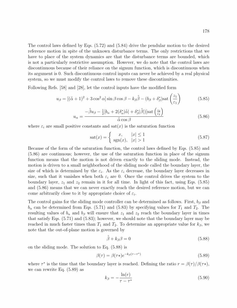
178

The control laws defined by Eqs. (5.72) and (5.84) drive the pendular motion to the desiredreference motion in spite of the unknown disturbance terms. The only restrictions that wehave to place of the system dynamics are that the disturbance terms are bounded, whichis not a particularly restrictive assumption. However, we do note that the control laws arediscontinuous because of their reliance on the signum function, which is discontinuous whenits argument is 0. Such discontinuous control inputs can never be achieved by a real physicalsystem, so we must modify the control laws to remove these discontinuities.

Following Refs. [58] and [28], let the control inputs have the modified form


β − (bβ + δ∗β)sat

(z1

ε1

)(5.85)

uα =−βuβ − 1

2[bα + 2(δ∗α|

α|+ δ∗β|

β|)]sat

(z2ε2

)α cos β

(5.86)

where εi are small positive constants and sat(x) is the saturation function

sat(x) =

x, |x| ≤ 1

sgn(x), |x| > 1(5.87)

Because of the form of the saturation function, the control laws defined by Eqs. (5.85) and(5.86) are continuous; however, the use of the saturation function in place of the signumfunction means that the motion is not driven exactly to the sliding mode. Instead, themotion is driven to a small neighborhood of the sliding mode called the boundary layer, thesize of which is determined by the εi. As the εi decrease, the boundary layer decreases insize, such that it vanishes when both εi are 0. Once the control drives the system to theboundary layer, z1 and z2 remain in it for all time. In light of this fact, using Eqs. (5.85)and (5.86) means that we can never exactly reach the desired reference motion, but we cancome arbitrarily close to it by appropriate choice of εi.

The control gains for the sliding mode controller can be determined as follows. First, bβ andbα can be determined from Eqs. (5.71) and (5.83) by specifying values for T1 and T2. Theresulting values of bα and bβ will ensure that z1 and z2 reach the boundary layer in timesthat satisfy Eqs. (5.71) and (5.83); however, we should note that the boundary layer may bereached in much faster times than T1 and T2. To determine an appropriate value for kβ, wenote that the out-of-plane motion is governed by

β + kββ = 0 (5.88)

on the sliding mode. The solution to Eq. (5.88) is

β(τ) = β(τ∗)e−kβ(τ−τ∗) (5.89)

where τ ∗ is the time that the boundary layer is reached. Defining the ratio r = β(τ)/β(τ∗),we can rewrite Eq. (5.89) as

kβ = − ln(r)

τ − τ ∗(5.90)

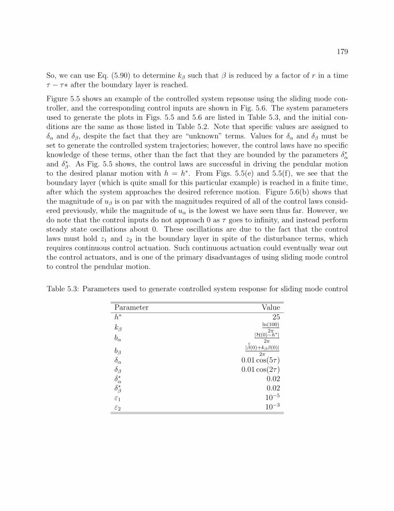
179

So, we can use Eq. (5.90) to determine kβ such that β is reduced by a factor of r in a timeτ − τ∗ after the boundary layer is reached.

Figure 5.5 shows an example of the controlled system repsonse using the sliding mode con-troller, and the corresponding control inputs are shown in Fig. 5.6. The system parametersused to generate the plots in Figs. 5.5 and 5.6 are listed in Table 5.3, and the initial con-ditions are the same as those listed in Table 5.2. Note that specific values are assigned toδα and δβ, despite the fact that they are “unknown” terms. Values for δα and δβ must beset to generate the controlled system trajectories; however, the control laws have no specificknowledge of these terms, other than the fact that they are bounded by the parameters δ∗αand δ∗β. As Fig. 5.5 shows, the control laws are successful in driving the pendular motionto the desired planar motion with h = h∗. From Figs. 5.5(e) and 5.5(f), we see that theboundary layer (which is quite small for this particular example) is reached in a finite time,after which the system approaches the desired reference motion. Figure 5.6(b) shows thatthe magnitude of uβ is on par with the magnitudes required of all of the control laws consid-ered previously, while the magnitude of uα is the lowest we have seen thus far. However, wedo note that the control inputs do not approach 0 as τ goes to infinity, and instead performsteady state oscillations about 0. These oscillations are due to the fact that the controllaws must hold z1 and z2 in the boundary layer in spite of the disturbance terms, whichrequires continuous control actuation. Such continuous actuation could eventually wear outthe control actuators, and is one of the primary disadvantages of using sliding mode controlto control the pendular motion.

Table 5.3: Parameters used to generate controlled system response for sliding mode control


kβln(100)

2π

bα|H(0)−h∗|

2π

bβ|β(0)+kββ(0)|

2π

δα 0.01 cos(5τ)δβ 0.01 cos(2τ)δ∗α 0.02δ∗β 0.02ε1 10−5

ε2 10−3

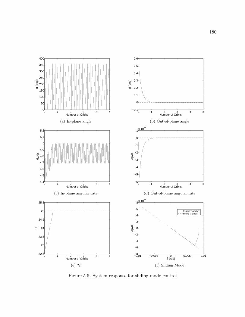
180

0 1 2 3 4 50

50

100

150

200

250

300

350

400

Number of Orbits

α (d

eg)

(a) In-plane angle

0 1 2 3 4 5−0.1

0

0.1

0.2

0.3

0.4

0.5

0.6

Number of Orbits

β (d

eg)


0 1 2 3 4 54.4

4.5

4.6

4.7

4.8

4.9

5

5.1

5.2

Number of Orbits

dα/d

τ


0 1 2 3 4 5−6

−5

−4

−3

−2

−1

0

1x 10−3

Number of Orbits

dβ/d

τ


0 1 2 3 4 522.5

23

23.5

24

24.5

25

25.5

Number of Orbits

H

(e) H

−0.01 −0.005 0 0.005 0.01−8

−6

−4

−2

0

2

4

6

8x 10−3

β (rad)

dβ/d

τ

System TrajectorySliding Manifold

(f) Sliding Mode

Figure 5.5: System response for sliding mode control

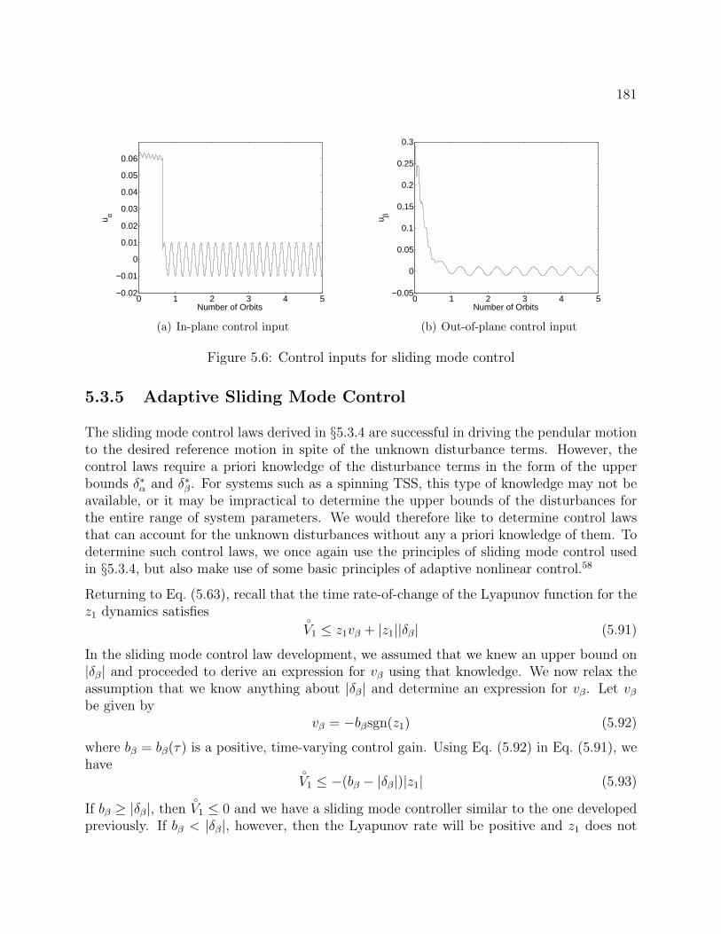
181

0 1 2 3 4 5−0.02

−0.01

0

0.01

0.02

0.03

0.04

0.05

0.06

Number of Orbits

u α


0 1 2 3 4 5−0.05

0

0.05

0.1

0.15

0.2

0.25

0.3

Number of Orbits

u β


Figure 5.6: Control inputs for sliding mode control

5.3.5 Adaptive Sliding Mode Control

The sliding mode control laws derived in §5.3.4 are successful in driving the pendular motionto the desired reference motion in spite of the unknown disturbance terms. However, thecontrol laws require a priori knowledge of the disturbance terms in the form of the upperbounds δ∗α and δ∗β. For systems such as a spinning TSS, this type of knowledge may not beavailable, or it may be impractical to determine the upper bounds of the disturbances forthe entire range of system parameters. We would therefore like to determine control lawsthat can account for the unknown disturbances without any a priori knowledge of them. Todetermine such control laws, we once again use the principles of sliding mode control usedin §5.3.4, but also make use of some basic principles of adaptive nonlinear control.58

Returning to Eq. (5.63), recall that the time rate-of-change of the Lyapunov function for thez1 dynamics satisfies

V1 ≤ z1vβ + |z1||δβ| (5.91)

In the sliding mode control law development, we assumed that we knew an upper bound on|δβ| and proceeded to derive an expression for vβ using that knowledge. We now relax theassumption that we know anything about |δβ| and determine an expression for vβ. Let vβbe given by

vβ = −bβsgn(z1) (5.92)

where bβ = bβ(τ) is a positive, time-varying control gain. Using Eq. (5.92) in Eq. (5.91), wehave

V1 ≤ −(bβ − |δβ|)|z1| (5.93)

If bβ ≥ |δβ|, thenV1 ≤ 0 and we have a sliding mode controller similar to the one developed

previously. If bβ < |δβ|, however, then the Lyapunov rate will be positive and z1 does not

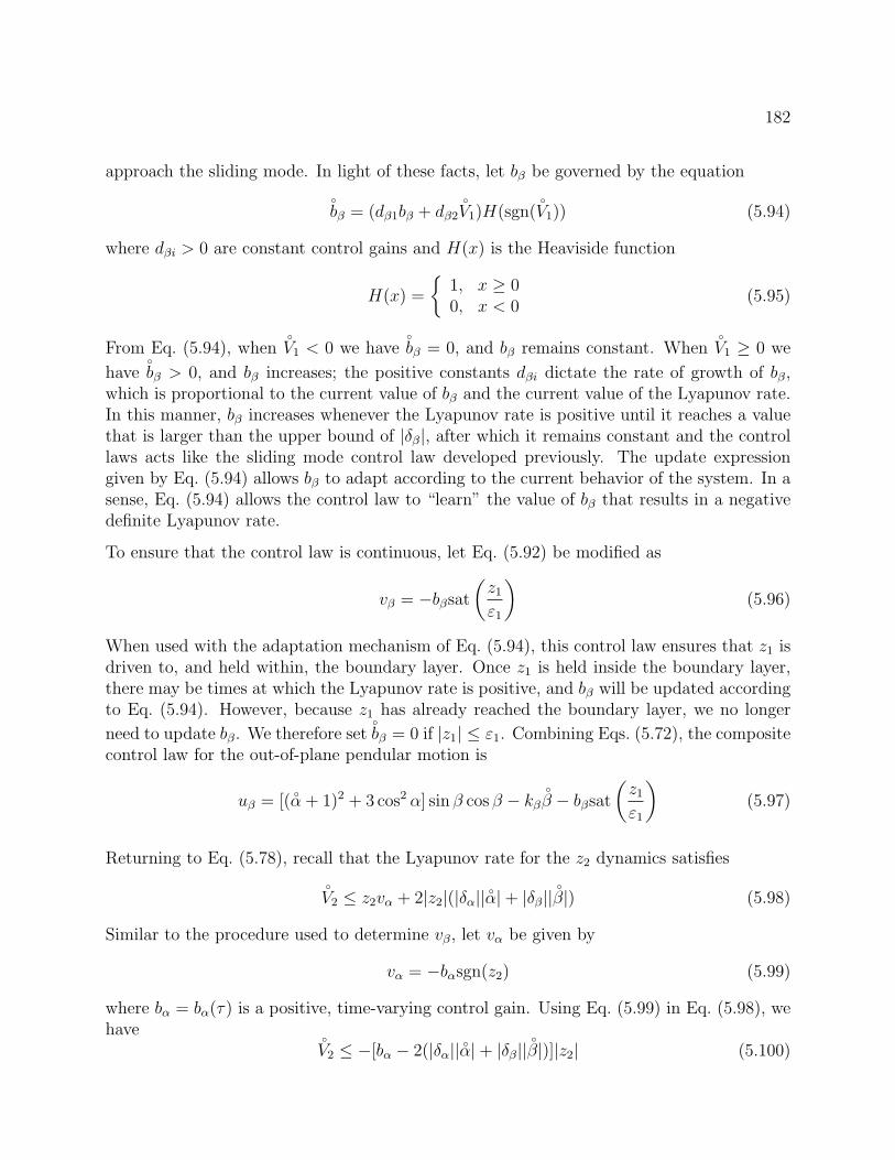
182

approach the sliding mode. In light of these facts, let bβ be governed by the equation

bβ = (dβ1bβ + dβ2

V1)H(sgn(

V1)) (5.94)

where dβi > 0 are constant control gains and H(x) is the Heaviside function

H(x) =

1, x ≥ 00, x < 0

(5.95)

From Eq. (5.94), whenV1 < 0 we have

bβ = 0, and bβ remains constant. When

V1 ≥ 0 we

havebβ > 0, and bβ increases; the positive constants dβi dictate the rate of growth of bβ,

which is proportional to the current value of bβ and the current value of the Lyapunov rate.In this manner, bβ increases whenever the Lyapunov rate is positive until it reaches a valuethat is larger than the upper bound of |δβ|, after which it remains constant and the controllaws acts like the sliding mode control law developed previously. The update expressiongiven by Eq. (5.94) allows bβ to adapt according to the current behavior of the system. In asense, Eq. (5.94) allows the control law to “learn” the value of bβ that results in a negativedefinite Lyapunov rate.

To ensure that the control law is continuous, let Eq. (5.92) be modified as

vβ = −bβsat

(z1

ε1

)(5.96)

When used with the adaptation mechanism of Eq. (5.94), this control law ensures that z1 isdriven to, and held within, the boundary layer. Once z1 is held inside the boundary layer,there may be times at which the Lyapunov rate is positive, and bβ will be updated accordingto Eq. (5.94). However, because z1 has already reached the boundary layer, we no longer

need to update bβ. We therefore setbβ = 0 if |z1| ≤ ε1. Combining Eqs. (5.72), the composite

control law for the out-of-plane pendular motion is


β − bβsat

(z1

ε1

)(5.97)

Returning to Eq. (5.78), recall that the Lyapunov rate for the z2 dynamics satisfies

V2 ≤ z2vα + 2|z2|(|δα||

α|+ |δβ||

β|) (5.98)

Similar to the procedure used to determine vβ, let vα be given by

vα = −bαsgn(z2) (5.99)

where bα = bα(τ) is a positive, time-varying control gain. Using Eq. (5.99) in Eq. (5.98), wehave

V2 ≤ −[bα − 2(|δα||

α|+ |δβ||

β|)]|z2| (5.100)

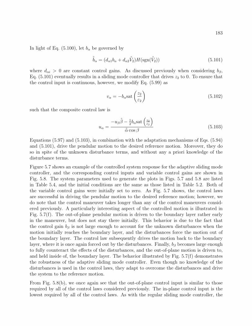
183

In light of Eq. (5.100), let bα be governed by

bα = (dα1bα + dα2

V2)H(sgn(

V2)) (5.101)

where dαi > 0 are constant control gains. As discussed previously when considering bβ,Eq. (5.101) eventually results in a sliding mode controller that drives z2 to 0. To ensure thatthe control input is continuous, however, we modify Eq. (5.99) as

vα = −bαsat

(z2

ε2

)(5.102)

such that the composite control law is

uα =−uβ

β − 1

2bαsat

(z2ε2

)α cos β

(5.103)

Equations (5.97) and (5.103), in combination with the adaptation mechanisms of Eqs. (5.94)and (5.101), drive the pendular motion to the desired reference motion. Moreover, they doso in spite of the unknown disturbance terms, and without any a priori knowledge of thedisturbance terms.

Figure 5.7 shows an example of the controlled system response for the adaptive sliding modecontroller, and the corresponding control inputs and variable control gains are shown inFig. 5.8. The system parameters used to generate the plots in Figs. 5.7 and 5.8 are listedin Table 5.4, and the initial conditions are the same as those listed in Table 5.2. Both ofthe variable control gains were initially set to zero. As Fig. 5.7 shows, the control lawsare successful in driving the pendular motion to the desired reference motion; however, wedo note that the control maneuver takes longer than any of the control maneuvers consid-ered previously. A particularly interesting aspect of the controlled motion is illustrated inFig. 5.7(f). The out-of-plane pendular motion is driven to the boundary layer rather earlyin the maneuver, but does not stay there initially. This behavior is due to the fact thatthe control gain bβ is not large enough to account for the unknown disturbances when themotion initially reaches the boundary layer, and the disturbances force the motion out ofthe boundary layer. The control law subsequently drives the motion back to the boundarylayer, where it is once again forced out by the disturbances. Finally, bβ becomes large enoughto fully counteract the effects of the disturbances, and the out-of-plane motion is driven to,and held inside of, the boundary layer. The behavior illustrated by Fig. 5.7(f) demonstratesthe robustness of the adaptive sliding mode controller. Even though no knowledge of thedisturbances is used in the control laws, they adapt to overcome the disturbances and drivethe system to the reference motion.

From Fig. 5.8(b), we once again see that the out-of-plane control input is similar to thoserequired by all of the control laws considered previously. The in-plane control input is thelowest required by all of the control laws. As with the regular sliding mode controller, the

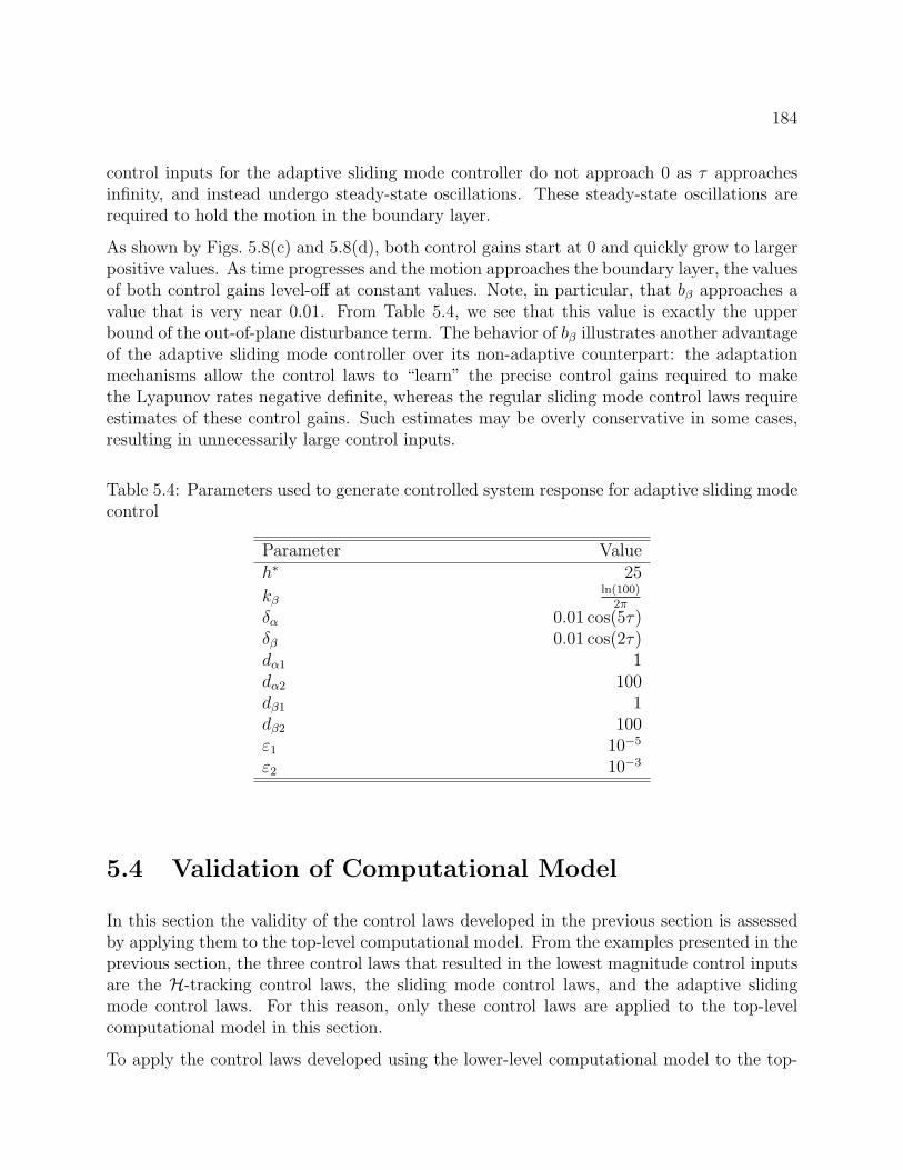
184

control inputs for the adaptive sliding mode controller do not approach 0 as τ approachesinfinity, and instead undergo steady-state oscillations. These steady-state oscillations arerequired to hold the motion in the boundary layer.

As shown by Figs. 5.8(c) and 5.8(d), both control gains start at 0 and quickly grow to largerpositive values. As time progresses and the motion approaches the boundary layer, the valuesof both control gains level-off at constant values. Note, in particular, that bβ approaches avalue that is very near 0.01. From Table 5.4, we see that this value is exactly the upperbound of the out-of-plane disturbance term. The behavior of bβ illustrates another advantageof the adaptive sliding mode controller over its non-adaptive counterpart: the adaptationmechanisms allow the control laws to “learn” the precise control gains required to makethe Lyapunov rates negative definite, whereas the regular sliding mode control laws requireestimates of these control gains. Such estimates may be overly conservative in some cases,resulting in unnecessarily large control inputs.

Table 5.4: Parameters used to generate controlled system response for adaptive sliding modecontrol


kβln(100)

2π

δα 0.01 cos(5τ)δβ 0.01 cos(2τ)dα1 1dα2 100dβ1 1dβ2 100ε1 10−5

ε2 10−3

5.4 Validation of Computational Model

In this section the validity of the control laws developed in the previous section is assessedby applying them to the top-level computational model. From the examples presented in theprevious section, the three control laws that resulted in the lowest magnitude control inputsare the H-tracking control laws, the sliding mode control laws, and the adaptive slidingmode control laws. For this reason, only these control laws are applied to the top-levelcomputational model in this section.

To apply the control laws developed using the lower-level computational model to the top-

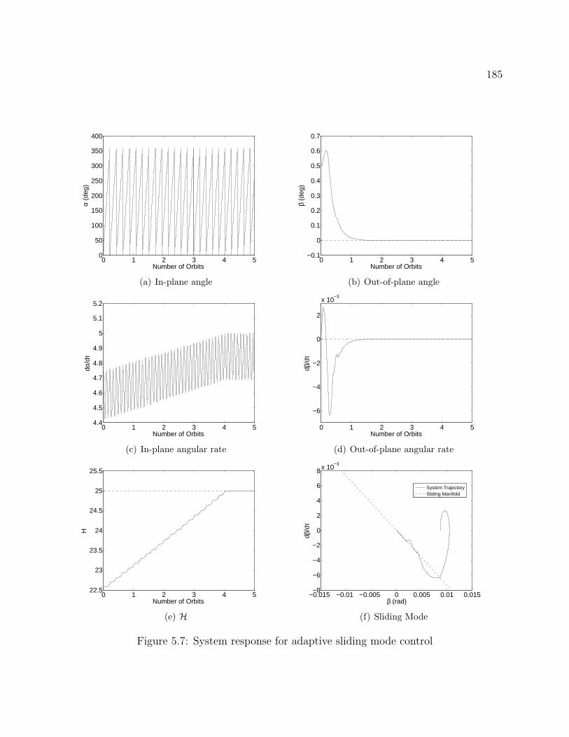
185

0 1 2 3 4 50

50

100

150

200

250

300

350

400

Number of Orbits

α (d

eg)

(a) In-plane angle

0 1 2 3 4 5−0.1

0

0.1

0.2

0.3

0.4

0.5

0.6

0.7

Number of Orbits

β (d

eg)


0 1 2 3 4 54.4

4.5

4.6

4.7

4.8

4.9

5

5.1

5.2

Number of Orbits

dα/d

τ


0 1 2 3 4 5

−6

−4

−2

0

2

x 10−3

Number of Orbits

dβ/d

τ


0 1 2 3 4 522.5

23

23.5

24

24.5

25

25.5

Number of Orbits

H

(e) H

−0.015 −0.01 −0.005 0 0.005 0.01 0.015−8

−6

−4

−2

0

2

4

6

8x 10−3

β (rad)

dβ/d

τ

System TrajectorySliding Manifold

(f) Sliding Mode

Figure 5.7: System response for adaptive sliding mode control

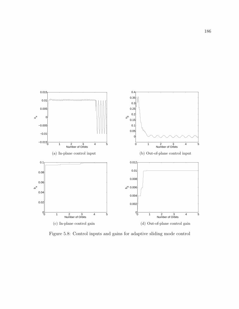
186

0 1 2 3 4 5−0.015

−0.01

−0.005

0

0.005

0.01

0.015

Number of Orbits

u α


0 1 2 3 4 5

0

0.05

0.1

0.15

0.2

0.25

0.3

0.35

0.4

Number of Orbits

u β


0 1 2 3 4 50

0.02

0.04

0.06

0.08

0.1

Number of Orbits

b α

(c) In-plane control gain

0 1 2 3 4 50

0.002

0.004

0.006

0.008

0.01

0.012

Number of Orbits

b β

(d) Out-of-plane control gain

Figure 5.8: Control inputs and gains for adaptive sliding mode control

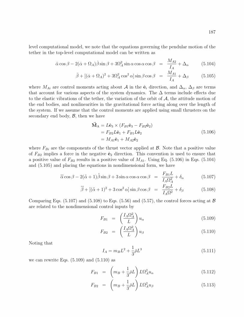
187

level computational model, we note that the equations governing the pendular motion of thetether in the top-level computational model can be written as

α cos β − 2(α + ΩA)β sin β + 3Ω2A sinα cosα cos β =

MA2

IA+ ∆α (5.104)

β + [(α + ΩA)2 + 3Ω2A cos2 α] sin β cos β =

MA1

IA+ ∆β (5.105)

where MAi are control moments acting about A in the ei direction, and ∆α, ∆β are termsthat account for various aspects of the system dynamics. The ∆ terms include effects dueto the elastic vibrations of the tether, the variation of the orbit of A, the attitude motion ofthe end bodies, and nonlinearities in the gravitational force acting along over the length ofthe system. If we assume that the control moments are applied using small thrusters on thesecondary end body, B, then we have

~MA = Le3 × (FB1e3 − FB2e2)

= FB2Le1 + FB1Le2

= MA1e1 +MA2e2

(5.106)

where FBi are the components of the thrust vector applied at B. Note that a positive valueof FB2 implies a force in the negative e2 direction. This convention is used to ensure thata positive value of FB2 results in a positive value of MA1. Using Eq. (5.106) in Eqs. (5.104)and (5.105) and placing the equations in nondimensional form, we have

α cos β − 2(

α + 1)

β sin β + 3 sinα cosα cos β =

FB1L

IAΩ2A

+ δα (5.107)

β + [(

α + 1)2 + 3 cos2 α] sin β cos β =

FB2L

IAΩ2+ δβ (5.108)

Comparing Eqs. (5.107) and (5.108) to Eqs. (5.56) and (5.57), the control forces acting at Bare related to the nondimensional control inputs by

FB1 =

(IAΩ2

A

L

)uα (5.109)

FB2 =

(IAΩ2

A

L

)uβ (5.110)

Noting that

IA = mBL2 +

1

3ρL3 (5.111)

we can rewrite Eqs. (5.109) and (5.110) as

FB1 =

(mB +

1

3ρL

)LΩ2

Auα (5.112)

FB2 =

(mB +

1

3ρL

)LΩ2

Auβ (5.113)

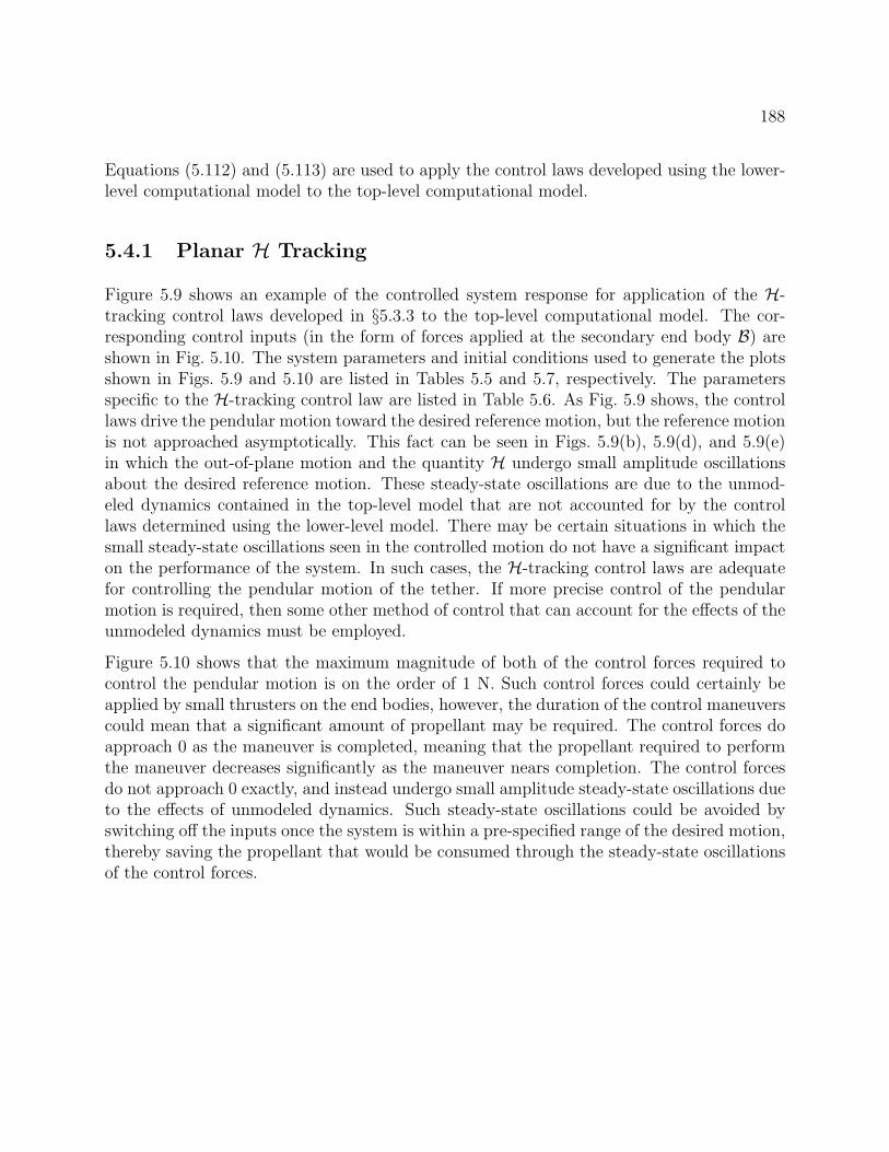
188

Equations (5.112) and (5.113) are used to apply the control laws developed using the lower-level computational model to the top-level computational model.

5.4.1 Planar H Tracking

Figure 5.9 shows an example of the controlled system response for application of the H-tracking control laws developed in §5.3.3 to the top-level computational model. The cor-responding control inputs (in the form of forces applied at the secondary end body B) areshown in Fig. 5.10. The system parameters and initial conditions used to generate the plotsshown in Figs. 5.9 and 5.10 are listed in Tables 5.5 and 5.7, respectively. The parametersspecific to the H-tracking control law are listed in Table 5.6. As Fig. 5.9 shows, the controllaws drive the pendular motion toward the desired reference motion, but the reference motionis not approached asymptotically. This fact can be seen in Figs. 5.9(b), 5.9(d), and 5.9(e)in which the out-of-plane motion and the quantity H undergo small amplitude oscillationsabout the desired reference motion. These steady-state oscillations are due to the unmod-eled dynamics contained in the top-level model that are not accounted for by the controllaws determined using the lower-level model. There may be certain situations in which thesmall steady-state oscillations seen in the controlled motion do not have a significant impacton the performance of the system. In such cases, the H-tracking control laws are adequatefor controlling the pendular motion of the tether. If more precise control of the pendularmotion is required, then some other method of control that can account for the effects of theunmodeled dynamics must be employed.

Figure 5.10 shows that the maximum magnitude of both of the control forces required tocontrol the pendular motion is on the order of 1 N. Such control forces could certainly beapplied by small thrusters on the end bodies, however, the duration of the control maneuverscould mean that a significant amount of propellant may be required. The control forces doapproach 0 as the maneuver is completed, meaning that the propellant required to performthe maneuver decreases significantly as the maneuver nears completion. The control forcesdo not approach 0 exactly, and instead undergo small amplitude steady-state oscillations dueto the effects of unmodeled dynamics. Such steady-state oscillations could be avoided byswitching off the inputs once the system is within a pre-specified range of the desired motion,thereby saving the propellant that would be consumed through the steady-state oscillationsof the control forces.

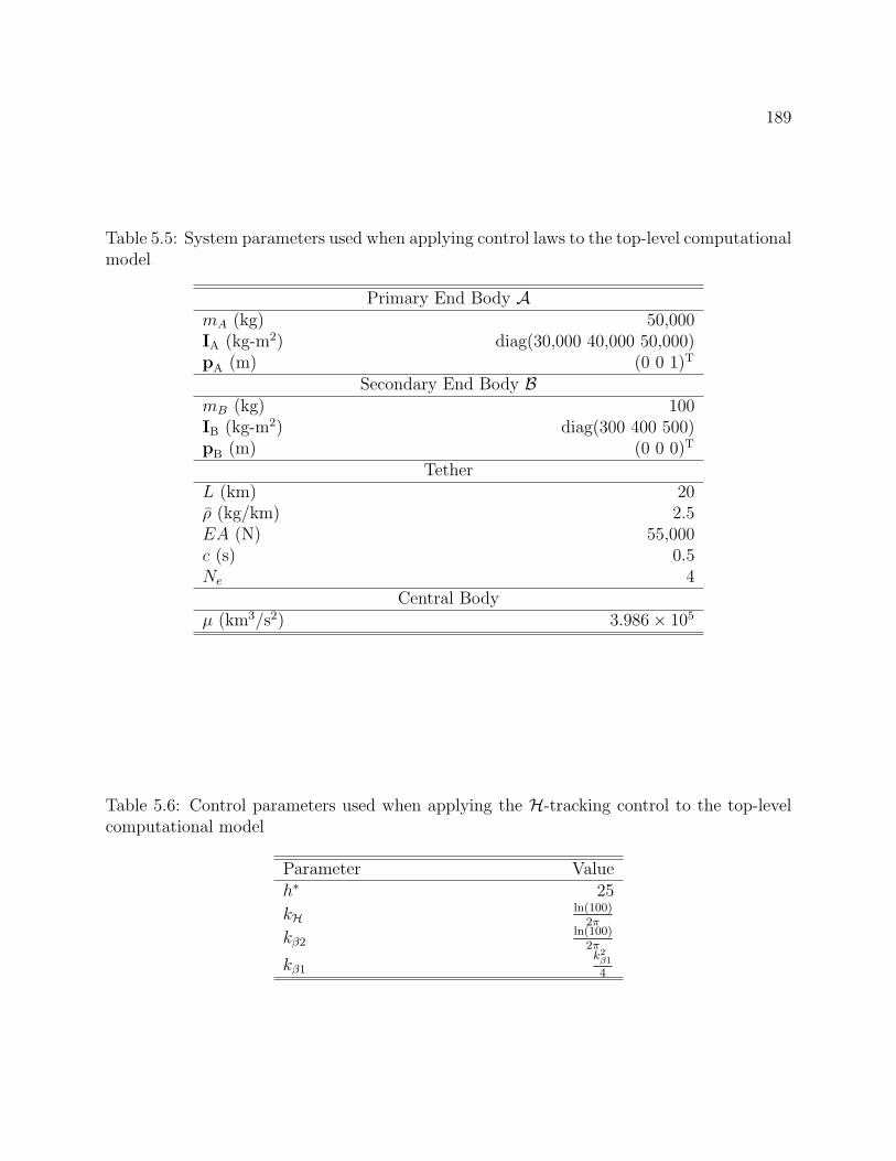
189

Table 5.5: System parameters used when applying control laws to the top-level computationalmodel


Secondary End Body BmB (kg) 100IB (kg-m2) diag(300 400 500)pB (m) (0 0 0)T



Table 5.6: Control parameters used when applying the H-tracking control to the top-levelcomputational model


kHln(100)

2π

kβ2ln(100)

2π

kβ1k2β1

4

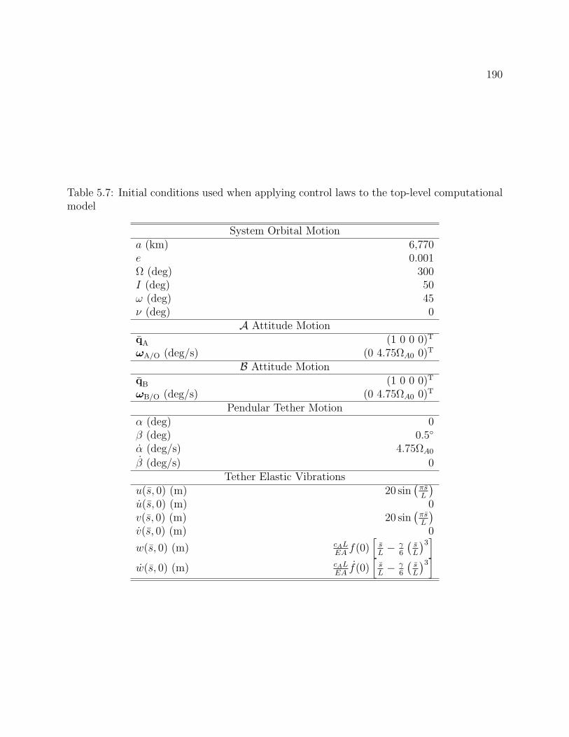
190

Table 5.7: Initial conditions used when applying control laws to the top-level computationalmodel



ωA/O (deg/s) (0 4.75ΩA0 0)T


ωB/O (deg/s) (0 4.75ΩA0 0)T

Pendular Tether Motionα (deg) 0β (deg) 0.5

α (deg/s) 4.75ΩA0



)u(s, 0) (m) 0v(s, 0) (m) 20 sin

(πsL

)v(s, 0) (m) 0

w(s, 0) (m) cALEA

f(0)[sL− γ

6

(sL

)3]

w(s, 0) (m) cALEA

f(0)[sL− γ

6

(sL

)3]

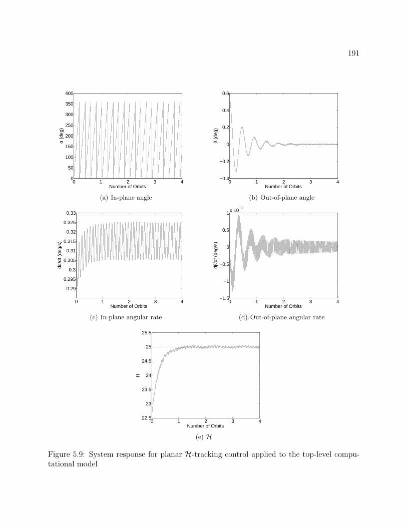
191

0 1 2 3 40

50

100

150

200

250

300

350

400

Number of Orbits

α (d

eg)

(a) In-plane angle

0 1 2 3 4−0.4

−0.2

0

0.2

0.4

0.6

Number of Orbits

β (d

eg)


0 1 2 3 4

0.29

0.295

0.3

0.305

0.31

0.315

0.32

0.325

0.33

Number of Orbits

dα/d

t (de

g/s)


0 1 2 3 4−1.5

−1

−0.5

0

0.5

1x 10−3

Number of Orbits

dβ/d

t (de

g/s)


0 1 2 3 422.5

23

23.5

24

24.5

25

25.5

Number of Orbits

H

(e) H

Figure 5.9: System response for planar H-tracking control applied to the top-level compu-tational model

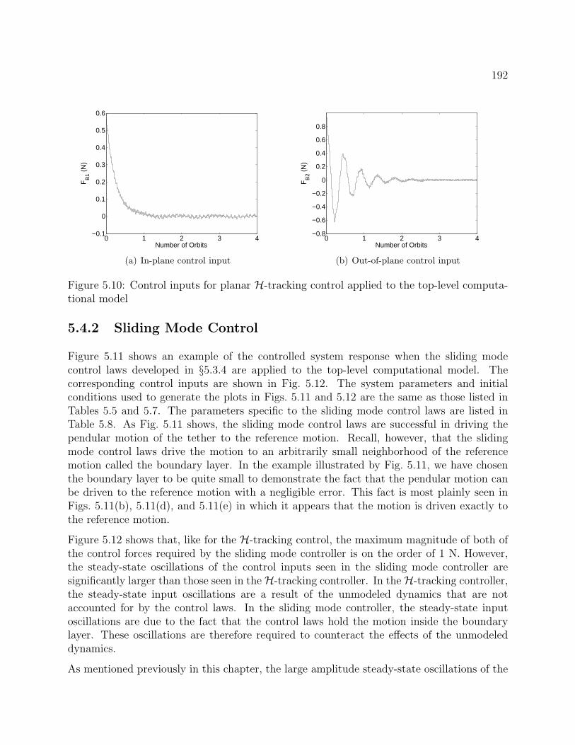
192

0 1 2 3 4−0.1

0

0.1

0.2

0.3

0.4

0.5

0.6

Number of Orbits

FB

1 (N

)


0 1 2 3 4−0.8

−0.6

−0.4

−0.2

0

0.2

0.4

0.6

0.8

Number of Orbits

FB

2 (N

)


Figure 5.10: Control inputs for planar H-tracking control applied to the top-level computa-tional model

5.4.2 Sliding Mode Control

Figure 5.11 shows an example of the controlled system response when the sliding modecontrol laws developed in §5.3.4 are applied to the top-level computational model. Thecorresponding control inputs are shown in Fig. 5.12. The system parameters and initialconditions used to generate the plots in Figs. 5.11 and 5.12 are the same as those listed inTables 5.5 and 5.7. The parameters specific to the sliding mode control laws are listed inTable 5.8. As Fig. 5.11 shows, the sliding mode control laws are successful in driving thependular motion of the tether to the reference motion. Recall, however, that the slidingmode control laws drive the motion to an arbitrarily small neighborhood of the referencemotion called the boundary layer. In the example illustrated by Fig. 5.11, we have chosenthe boundary layer to be quite small to demonstrate the fact that the pendular motion canbe driven to the reference motion with a negligible error. This fact is most plainly seen inFigs. 5.11(b), 5.11(d), and 5.11(e) in which it appears that the motion is driven exactly tothe reference motion.

Figure 5.12 shows that, like for the H-tracking control, the maximum magnitude of both ofthe control forces required by the sliding mode controller is on the order of 1 N. However,the steady-state oscillations of the control inputs seen in the sliding mode controller aresignificantly larger than those seen in theH-tracking controller. In theH-tracking controller,the steady-state input oscillations are a result of the unmodeled dynamics that are notaccounted for by the control laws. In the sliding mode controller, the steady-state inputoscillations are due to the fact that the control laws hold the motion inside the boundarylayer. These oscillations are therefore required to counteract the effects of the unmodeleddynamics.

As mentioned previously in this chapter, the large amplitude steady-state oscillations of the

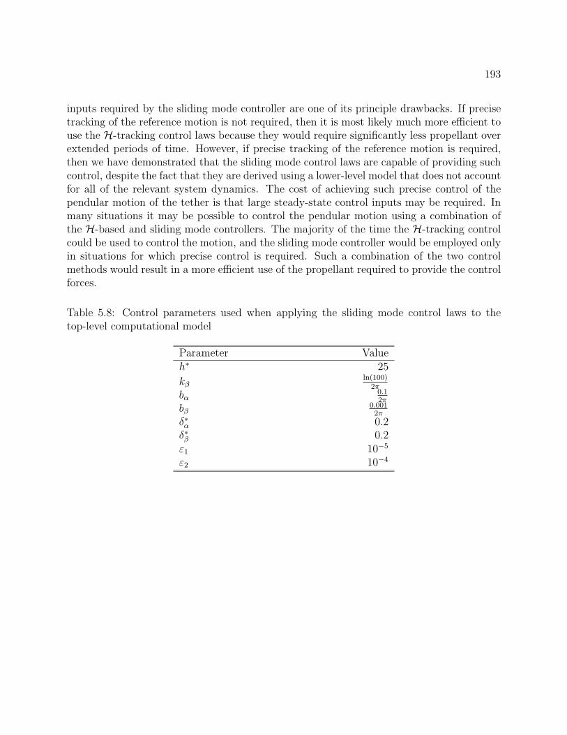
193

inputs required by the sliding mode controller are one of its principle drawbacks. If precisetracking of the reference motion is not required, then it is most likely much more efficient touse the H-tracking control laws because they would require significantly less propellant overextended periods of time. However, if precise tracking of the reference motion is required,then we have demonstrated that the sliding mode control laws are capable of providing suchcontrol, despite the fact that they are derived using a lower-level model that does not accountfor all of the relevant system dynamics. The cost of achieving such precise control of thependular motion of the tether is that large steady-state control inputs may be required. Inmany situations it may be possible to control the pendular motion using a combination ofthe H-based and sliding mode controllers. The majority of the time the H-tracking controlcould be used to control the motion, and the sliding mode controller would be employed onlyin situations for which precise control is required. Such a combination of the two controlmethods would result in a more efficient use of the propellant required to provide the controlforces.

Table 5.8: Control parameters used when applying the sliding mode control laws to thetop-level computational model


kβln(100)

2π

bα0.12π

bβ0.001

2π

δ∗α 0.2δ∗β 0.2ε1 10−5

ε2 10−4

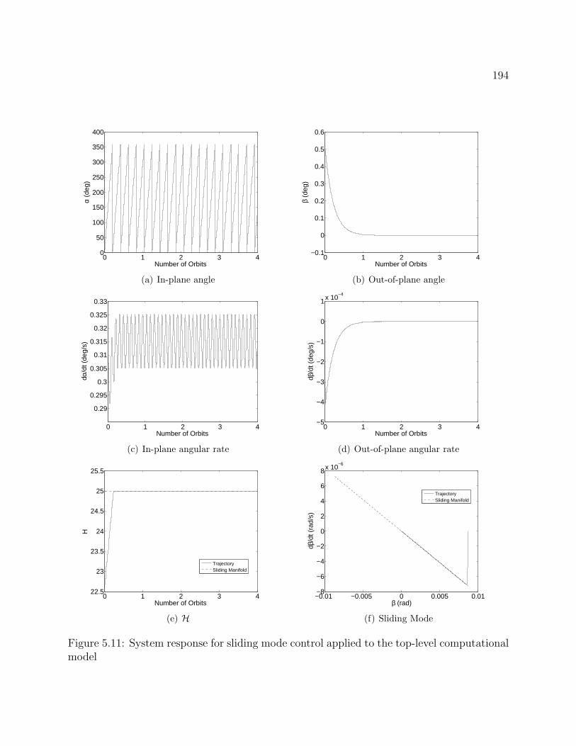
194

0 1 2 3 40

50

100

150

200

250

300

350

400

Number of Orbits

α (d

eg)

(a) In-plane angle

0 1 2 3 4−0.1

0

0.1

0.2

0.3

0.4

0.5

0.6

Number of Orbits

β (d

eg)


0 1 2 3 4

0.29

0.295

0.3

0.305

0.31

0.315

0.32

0.325

0.33

Number of Orbits

dα/d

t (de

g/s)


0 1 2 3 4−5

−4

−3

−2

−1

0

1x 10−4

Number of Orbits

dβ/d

t (de

g/s)


0 1 2 3 422.5

23

23.5

24

24.5

25

25.5

Number of Orbits

H

TrajectorySliding Manifold

(e) H

−0.01 −0.005 0 0.005 0.01−8

−6

−4

−2

0

2

4

6

8x 10−6

β (rad)

dβ/d

t (ra

d/s)


(f) Sliding Mode

Figure 5.11: System response for sliding mode control applied to the top-level computationalmodel

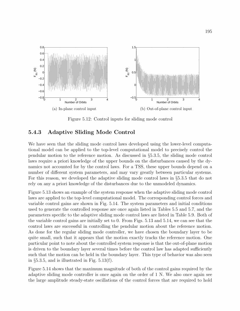
195

0 1 2 3 4−0.8

−0.6

−0.4

−0.2

0

0.2

0.4

0.6

0.8

Number of Orbits

FB

1 (N

)


0 1 2 3 4−0.5

0

0.5

1

1.5

Number of Orbits

FB

2 (N

)


Figure 5.12: Control inputs for sliding mode control

5.4.3 Adaptive Sliding Mode Control

We have seen that the sliding mode control laws developed using the lower-level computa-tional model can be applied to the top-level computational model to precisely control thependular motion to the reference motion. As discussed in §5.3.5, the sliding mode controllaws require a priori knowledge of the upper bounds on the disturbances caused by the dy-namics not accounted for by the control laws. For a TSS, these upper bounds depend on anumber of different system parameters, and may vary greatly between particular systems.For this reason, we developed the adaptive sliding mode control laws in §5.3.5 that do notrely on any a priori knowledge of the disturbances due to the unmodeled dynamics.

Figure 5.13 shows an example of the system response when the adaptive sliding mode controllaws are applied to the top-level computational model. The corresponding control forces andvariable control gains are shown in Fig. 5.14. The system parameters and initial conditionsused to generate the controlled response are once again listed in Tables 5.5 and 5.7, and theparameters specific to the adaptive sliding mode control laws are listed in Table 5.9. Both ofthe variable control gains are initially set to 0. From Figs. 5.13 and 5.14, we can see that thecontrol laws are successful in controlling the pendular motion about the reference motion.As done for the regular sliding mode controller, we have chosen the boundary layer to bequite small, such that it appears that the motion exactly tracks the reference motion. Oneparticular point to note about the controlled system response is that the out-of-plane motionis driven to the boundary layer several times before the control law has adapted sufficientlysuch that the motion can be held in the boundary layer. This type of behavior was also seenin §5.3.5, and is illustrated in Fig. 5.13(f).

Figure 5.14 shows that the maximum magnitude of both of the control gains required by theadaptive sliding mode controller is once again on the order of 1 N. We also once again seethe large amplitude steady-state oscillations of the control forces that are required to hold

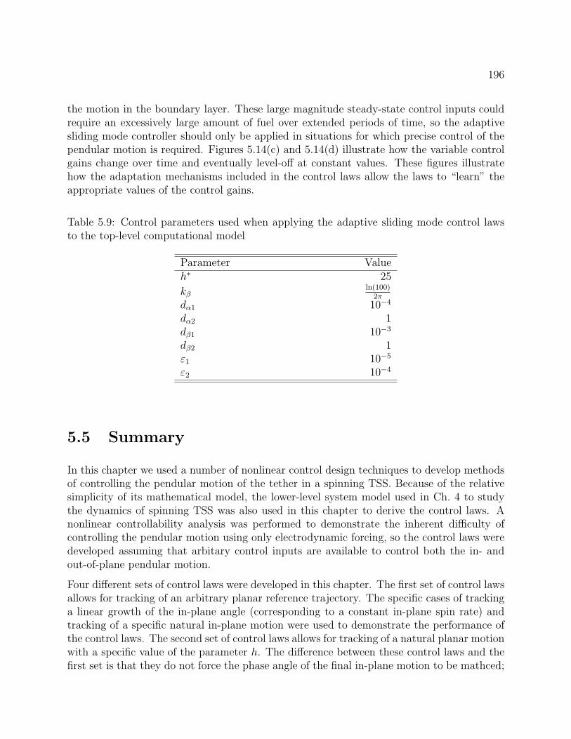
196

the motion in the boundary layer. These large magnitude steady-state control inputs couldrequire an excessively large amount of fuel over extended periods of time, so the adaptivesliding mode controller should only be applied in situations for which precise control of thependular motion is required. Figures 5.14(c) and 5.14(d) illustrate how the variable controlgains change over time and eventually level-off at constant values. These figures illustratehow the adaptation mechanisms included in the control laws allow the laws to “learn” theappropriate values of the control gains.

Table 5.9: Control parameters used when applying the adaptive sliding mode control lawsto the top-level computational model


kβln(100)

2π

dα1 10−4

dα2 1dβ1 10−3

dβ2 1ε1 10−5

ε2 10−4

5.5 Summary

In this chapter we used a number of nonlinear control design techniques to develop methodsof controlling the pendular motion of the tether in a spinning TSS. Because of the relativesimplicity of its mathematical model, the lower-level system model used in Ch. 4 to studythe dynamics of spinning TSS was also used in this chapter to derive the control laws. Anonlinear controllability analysis was performed to demonstrate the inherent difficulty ofcontrolling the pendular motion using only electrodynamic forcing, so the control laws weredeveloped assuming that arbitary control inputs are available to control both the in- andout-of-plane pendular motion.

Four different sets of control laws were developed in this chapter. The first set of control lawsallows for tracking of an arbitrary planar reference trajectory. The specific cases of trackinga linear growth of the in-plane angle (corresponding to a constant in-plane spin rate) andtracking of a specific natural in-plane motion were used to demonstrate the performance ofthe control laws. The second set of control laws allows for tracking of a natural planar motionwith a specific value of the parameter h. The difference between these control laws and thefirst set is that they do not force the phase angle of the final in-plane motion to be mathced;

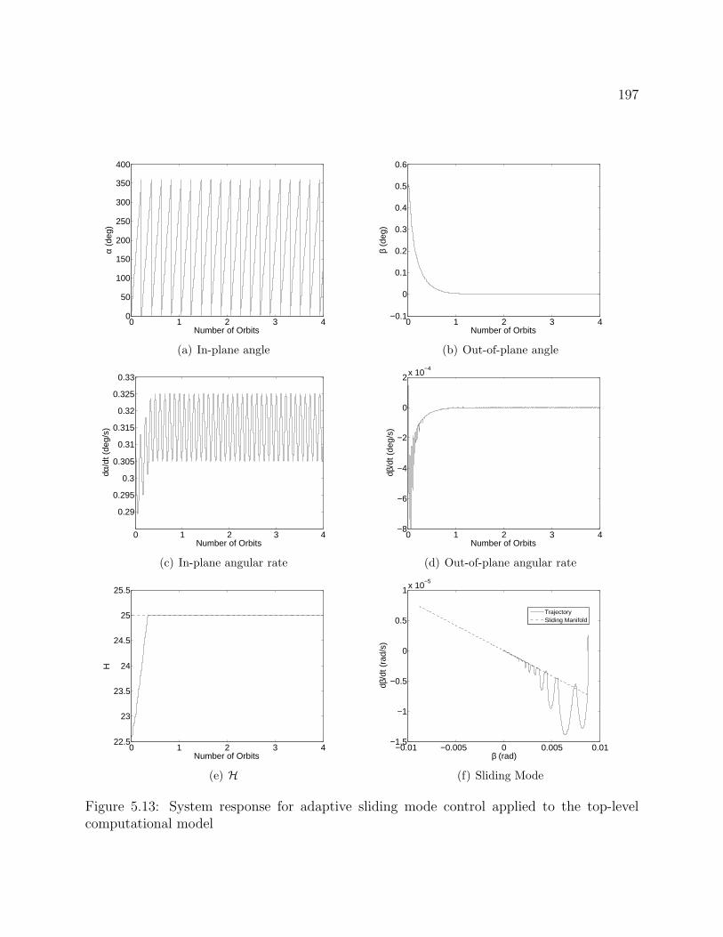
197

0 1 2 3 40

50

100

150

200

250

300

350

400

Number of Orbits

α (d

eg)

(a) In-plane angle

0 1 2 3 4−0.1

0

0.1

0.2

0.3

0.4

0.5

0.6

Number of Orbits

β (d

eg)


0 1 2 3 4

0.29

0.295

0.3

0.305

0.31

0.315

0.32

0.325

0.33

Number of Orbits

dα/d

t (de

g/s)


0 1 2 3 4−8

−6

−4

−2

0

2x 10−4

Number of Orbits

dβ/d

t (de

g/s)


0 1 2 3 422.5

23

23.5

24

24.5

25

25.5

Number of Orbits

H

(e) H

−0.01 −0.005 0 0.005 0.01−1.5

−1

−0.5

0

0.5

1x 10−5

β (rad)

dβ/d

t (ra

d/s)


(f) Sliding Mode

Figure 5.13: System response for adaptive sliding mode control applied to the top-levelcomputational model

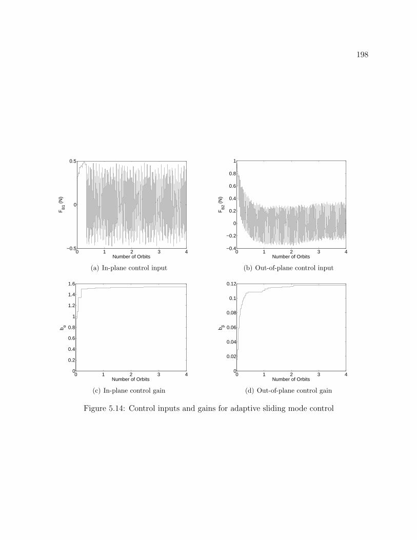
198

0 1 2 3 4−0.5

0

0.5

Number of Orbits

FB

1 (N

)


0 1 2 3 4−0.4

−0.2

0

0.2

0.4

0.6

0.8

1

Number of Orbits

FB

2 (N

)


0 1 2 3 40

0.2

0.4

0.6

0.8

1

1.2

1.4

1.6

Number of Orbits

b α

(c) In-plane control gain

0 1 2 3 40

0.02

0.04

0.06

0.08

0.1

0.12

Number of Orbits

b β

(d) Out-of-plane control gain

Figure 5.14: Control inputs and gains for adaptive sliding mode control

199

all that is matched is the value of h of the desired natural planar motion. In general, thefact that the phase angle is not matched results in lower control inputs than required whenthe phase angle is matched. The third set of control laws are based on principles of slidingmode control, meaning that they can control the pendular motion about a desired referencemotion in spite of the presence of unknown disturbance terms due to unmodeled dynamics.The only constraint required of these control laws is that the unknown disturbances arebounded, and that these bounds are known a priori. One of the main drawbacks of using thesliding mode control laws is that they can require relatively large steady-state control inputsto hold the system at the reference motion. The magnitude of these steady-state controlinputs depends on the magnitude of the disturbances, and they may become excessivelylarge for some systems. The fourth and final set of control laws developed in this chapteris an extension of the third set to include some principles of adaptive control. For a typicalTSS, it may be difficult or impractical to determine the bounds on the disturbance termsrequired by the sliding mode control laws. In light of this fact, the fourth set of controllaws includes adaptation mechanisms that allow the control gains included in the laws tostart at 0 and gradually “learn” what values they should be to compensate for the unknowndisturbances and drive the system to the reference motion. In this manner, precise controlof the pendular motion is achieved without any a priori knowledge of the disturbance terms.As with the regular sliding mode control laws, however, relatively large steady-state controlinputs can be required to compensate for the unknown disturbance terms.

The second, third, and fourth sets of control laws derived in this chapter were applied tothe top-level computational model to assess their applicability to an actual spinning TSS.The second set of control laws were successful in driving the pendular motion of the top-level computational model to the reference motion; however, the fact that the top-levelmodel contains dynamics that are not accounted for by the lower-level model results insmall steady-state oscillations about the reference motion. These steady-state oscillationscan be quite small, and could most likely be tolerated for many applications. Both sets ofsliding mode control laws were also successful in driving the pendular motion of the top-level computational model to the reference motion, but these control laws achieve muchmore precise tracking because of their ability to compensate for the effects of unmodeleddynamics. As mentioned previously, the main drawback of either set of sliding mode controllaws is that they require relatively large steady-state control inputs to compensate for theeffects of unmodeled dynamics. When applied to the top-level computational model, theselarge steady-state inputs translate to large propellant requirements for the thrusters on thesecondary end body that provide the control forces. In practice, a combination controlscheme incorporating the sliding mode control and the second set of control laws could beapplied to more efficiently manage the propellant required to control the pendular motion.The second set of control laws would be used for most situations for which less precise controlis needed, and the sliding mode control laws would only be used in situations that requireprecise control of the pendular motion.

Chapter 6

Summary and Recommendations forFuture Work

Tethered satellite systems have a great deal of potential for a wide range of future space-basedapplications. Although a great deal of research has already been conducted on the dynamicsand control of TSS, there remain a number of open areas of study that must be addressedbefore TSS can be widely put to use. The objective of the work presented in this dissertationis to address several of these open areas of study, and in the process identify new avenuesdown which TSS dynamics and control research should progress. The original contributionsprovided by this dissertation are summarized below, and we also present recommendationsfor future work on TSS dynamics and control.

6.1 Summary of Contributions

One of the main contributions provided by this dissertation is the computational model val-idation procedure presented in Ch. 2. In an ideal situation, the predictions made by thecomputational model for a particular physical system are compared to experimental datato assess the predictive capability of the computational model. For a TSS, such experimen-tal data does not exist, so some other means of validating TSS computational models isrequired. The validation procedure presented in Ch. 2 uses the output of a top-level compu-tational model in place of the non-existent experimental data. The conceptual model of thephysical system used to develop the top-level computational model must therefore containas few simplifying assumptions as possible, while still allowing for efficient determination ofnumerical solutions for the behavior of the system. The accuracy of the numerical solutionsproduced by the top-level computational model must also be rigorously verified before theycan be used to assess the validity of any predictions made using lower-level computationalmodels. The validation procedure presented in Ch. 2 is by no means ideal, most notably

200

201

because there is no guarantee that the top-level computational model itself makes accuratepredictions about the behavior of the physical system. Only experimental data can be usedto perform validation in the truest sense of the word, but we believe that the computationalmodel validation procedure presented in this work is the best available option for systems,like a TSS, for which experimental data is not available.

Motivated by the validation procedure outlined in Ch. 2, a top-level computational model forthe dynamics and control of TSS was developed in Ch. 3. The system was assumed to consistof two finite, rigid end bodies connected by a flexible tether. The tether is allowed to carry aconstant electrical current, meaning that the model can be used to analyze electrodynamictether systems. The mathematical model of the system was derived and used to develop twodifferent computational models, each based on a different method of spatially discretizingthe partial differential equations governing the elastic vibrations of the tether. The firstmethod is the assumed modes method, and the second method is the finite element method.Computer codes were written to produce numerical solutions for both computational models,and the method of manufactured solutions was used to verify the accuracy of these numericalsolutions. To the knowledge of the author, the work presented in Ch. 3 represents the firsttime that the MMS has been applied to a computational model for the dynamics and controlof a TSS. A qualitative comparison of the two computational models was made and it wasdetermined that the FEM-based computational model is better suited to the study of TSSdynamics and control. For this reason, the FEM-based computational model was used as thetop-level computational model for TSS dynamics and control throughout this dissertation.

Because of the complicated nature of the top-level system model, studying the behavior ofa TSS using the top-level computational model is impractical in most situations. Accuratenumerical solutions can take a significant amount of time to produce using the top-levelcomputational model, so studying the behavior of the system over the entire parameterspace can be practically impossible. For this reason, it is entirely justifiable to use simplifiedsystem models that allow for much easier analysis of the system. In Ch. 4, a lower-levelcomputational model was used to derive results related to the dynamics of the tether in aspinning TSS. The lower-level model treats the tether as two point mass end bodies connectedby a flexible tether, with the primary end body constrained to an unperturbed circular orbit.The pendular motion of the tether is assumed to affect the transverse vibrations of the tether,but the transverse vibrations are assumed to have no influence on the pendular motion. Thelongitudinal elastic vibrations of the tether are assumed to be negligible.

The nominal pendular motion of a spinning TSS is in the orbit plane, so the equationsgoverning the pendular motion of the tether in the lower-level mathematical model werelinearized about a planar motion. The resulting equation for the in-plane pendular motionis decoupled from the equation governing the out-of-plane pendular motion, and a solutionfor the in-plane motion is determined in terms of Jacobi elliptic functions. When this solutionfor the in-plane motion is used in the equation governing the out-of-plane motion, the result isa Hill’s equation, and Floquet theory was used to analyze the stability properties of the out-of-plane pendular motion. The Floquet analysis showed that the lower-level computational

202

model predicts that the out-of-plane pendular motion is unstable for some large-amplitudein-plane oscillatory motion, as well as ranges of rotational in-plane motion for systems withboth positive and negative in-plane spin rates. The instability regions for systems with anegative in-plane spin rate correspond to systems for which the tether undergoes periods ofslack, so they would likely not be used for an actual spinning TSS in spite of the unstableout-of-plane motion. However, the predicted instability regions for systems with a positivein-plane spin rate do not pass through periods of slackness, so they could have possibleapplication for an actual spinning TSS. If such a system were used, a great deal of controleffort would be required to counteract the effects of the unstable out-of-plane motion. Theinstabilities in the out-of-plane pendular motion derived in Ch. 4 have not been reportedpreviously, and are an original contribution of this dissertation.

For spinning TSS with relatively large in-plane spin rates, the Hill’s equation used to modelthe small out-of-plane pendular motion can be approximated with sufficient accuracy by aMathieu’s equation. Floquet’s theorem was used to determine approximate solutions to theMathieu’s equation that are a linear combination of four simple harmonic oscillators. Thetwo lowest-frequency oscillators contribute the greatest to the overall amplitude of the out-of-plane oscillations, and the frequency of all four of the oscillators increases as the in-planespin rate increases. Like the predicted instabilities in the out-of-plane pendular motion, theapproximate solutions for large in-plane spin rates have not been reported previously, andare an original contribution of this dissertation.

In addition to the pendular motion of the tether, the lower-level computational model wasused to study the transverse elastic vibrations of a spinning TSS. The transverse vibrationsare assumed to be small relative to the length of the tether, and the out-of-plane pendularmotion is once again assumed to be small. The resulting equations governing the transverseelastic vibrations are a set of decoupled, linear, partial differential equations, and the methodof separation of variables is used to analyze these equations. The mode shapes for thetransverse vibrations are determined in terms of a hypergeometric function, and an expressionfor the eigenvalue corresponding to each mode shape is determined. The eigenvalues andthe solution for the in-plane pendular motion are used in the equations governing the time-dependent portions of the assumed solution forms for the transverse vibrations, resultingin Hill’s equations. Floquet theory was used to analyze these equations and show thatthe lower-level computational model predicts that the transverse vibrations are unstablefor certain combinations of in-plane spin rate and system mass distribution. The largestinstability regions correspond to systems with a relatively low in-plane spin rate and asecondary end mass that is small relative to the mass of the tether. The instability regionsbecome progressively smaller as the in-plane spin rate and mass of the secondary end bodyare increased. Unlike the results related to the stability of the out-of-plane pendular motion,these results related to the instabilities in the transverse elastic vibrations of the tether arenot new, and were previously reported in Refs. [5] and [8].

Because they were determined using a lower-level computational model, the results related tothe motion of the tether in a spinning TSS presented in Ch. 4 were compared to predictions

203

made by the top-level computational model to assess their validity. Numerous validation testswere used to show that the instabilities in the out-of-plane pendular motion predicted by thelower-level computational model are also predicted by the top-level computational model,meaning that these predictions are validated. The approximate solutions for the out-of-planemotion compare favorably to the predictions made by the top-level computational model in aqualitative sense, but significant quantitative differences develop between the predictions overlonger time spans. These differences are due to slight errors in the approximate frequenciesthat, over time, lead to significant phase differences. Despite these quantitative differences,however, the approximate solutions accurately reproduce the qualitative features of the out-of-plane pendular motion predicted by the top-level computational model.

A number of validation tests were used to show that the instabilities in the transverseelastic vibrations of the tether predicted by the lower-level computational model are notpredicted by the top-level computational model. These results are therefore invalidated,and the lower-level system model must be altered to achieve better agreement with the top-level computational model. The main source of error in the lower-level predictions appearsto stem from the assumption of a one-way coupling between the two modes of the tethermotion. Any further study of the transverse vibrations of a spinning TSS should not usesuch an assumption, and should consider the transverse vibrations and pendular motion tobe completely coupled.

The validation tests presented in Ch. 4 are one of the most significant contributions providedby this dissertation. They show that predictions made by lower-level computational modelscan both agree and disagree with those made by the top-level computational model. If thepredictions made by the two models agree, then the lower-level predictions are given a weightand significance that they would not have if no kind of validation had been performed. If thepredictions made by the two models do not agree, then the lower-level system model must bealtered in some manner to achieve better agreement. The validation tests performed on theresults pertaining to the transverse elastic vibrations of the tether clearly demonstrate thatthe mathematical correctness of a prediction does not mean that it can, or should, be appliedto the physical system. Some form of validation must be performed to tie the predictionsback to the actual physical system in order for the predictions to have any real significance.

The final significant contribution made in this dissertation is the control laws for the pendularmotion of the tether developed in Ch. 5. All of these control laws were developed using alower-level system model, and all drive the pendular motion to a desired planar referencemotion. The control inputs used to control the pendular motion are assumed to be arbitrarycontrol torques that are most likely due to thrusters on the end bodies. Two of the controllaws developed in Ch. 5 are based on principles of sliding mode control, meaning that theycan control the system about the reference motion in the presence of unknown disturbances.When applied to the top-level computational model, these unknown disturbances are due tothe dynamics not accounted for by the lower-level model.

Several of the control laws were applied to the top-level computational model to assess their

204

applicability to an actual TSS. For the control laws that do not account for the unmodeledsystem dynamics, the pendular motion does not asymptotically approach the desired motion,but instead undergoes small amplitude oscillations about the desired reference motion dueto the effects of the unmodeled dynamics. The sliding mode control laws were demonstratedto be capable of eliminating these steady-state oscillations about the reference motion atthe cost of requiring relatively large magnitude steady-state control inputs. Because of thisfact, the sliding mode controllers should only be used in situations for which precise controlof the pendular motion is required. In most other situations, the control laws that do notaccount for unmodeled dynamics should prove sufficient in controlling the pendular motionof the tether.

6.2 Recommendations for Future Work

The work presented in this dissertation addresses only a handful of the open areas of researchin TSS dynamics and control. Many issues have yet to be adequately addressed, and thework in this dissertation raises several new questions on its own. In this section, we makerecommendations for ways in which the work presented in this dissertation can be extendedin future TSS dynamics and control research.

The first way in which the work in this dissertation can be extended is to refine the top-levelsystem model. Despite the fact that the system model presented in Ch. 3 is taken as thetop-level system model, it contains several assumptions about the physical system that couldbe relaxed to make the model a better abstraction of reality. Most of these assumptions arerelated to the physical environment in which the TSS operates; recall that the only externalforces acting on the system in the top-level system model are the gravitational force ofthe central body and the electrodynamic force. Other external forces, such as atmosphericdrag and solar radiation pressure, could be added to the model, along with other effectslike thermal expansion of the tether due to crossings between shadow and sunlight. Thegravitational and electrodynamic force models can themselves be extended by using higher-order spherical harmonic expansions of the gravitational and magnetic fields of the centralbody. Modeling all of these external forces would make the top-level system model a betterrepresentation of an actual TSS, and would therefore provide an even better substitute forexperimental data until it can be collected.

The fact that experimental data from an actual TSS is not readily available does not meanthat data cannot be collected to validate some aspects of the system model. For example,the string model for the tether can be applied to any type of vibrating string, not just aTSS. In light of this fact, experimental data collected on an experimental setup as simpleas a pendulum could be used to determine if a string model is adequate for modeling thevibrations of a TSS. Such experiments are conducted in Ref. [29]; however, comparisonwith the computational model is conducted by means of stop-motion photographs instead ofphysical measurements. More rigorous validation test than the ones conducted in Ref. [29]

205

would greatly enhance the level of confidence in modeling of TSS dynamics.

The dynamic analysis of spinning TSS presented in Ch. 4 can be extended in a number ofways. Many extensions of the system model used in Ch. 4 will result in equations that aresmall perturbations of those used in Ch.4. For example, orbital eccentricity and electrody-namic forcing introduce small perturbation terms into the equations governing the pendularmotion of the tether. The effects of these additional influences can be studied using variousperturbation methods (such as the method of averaging) with the solutions derived in Ch. 4as the generating solutions for the perturbation analysis. The variation of the system orbitdue to various external influences can also be studied by viewing the orbital motion as asmall perturbation of a fixed orbit. Another way in which the dynamic analysis in Ch. 4 canbe extended is to develop a new computational model for the elastic vibrations of the tetherthat takes into account the full coupling between the pendular motion and elastic vibrationsof the tether. It may be possible to derive analytical results on the stability of the transversevibrations using this new lower-level system model, but it is likely that any accurate studyof the elastic vibrations of the tether will have to rely on numerical solutions.

One significant way in which the control analysis presented in Ch. 5 can be extended isto perform a more thorough controllability analysis of the system for the case in which theelectrodynamic force is the only control input. It may be possible to perform certain types ofcontrol maneuvers using only the electrodynamic force, and knowing these maneuvers couldprove useful because they would require no propellant. Along the same lines, it would beuseful to determine optimal control laws that minimize the total control input required tocontrol the pendular motion, thereby minimizing the required propellant. Both open- andclosed-loop optimal control laws could be developed. Some hybrid control strategy couldbe developed that uses a combination of electrodynamic forcing and thrusters on the endbodies. The electrodynamic force could be used as the only control input for times whenthe pendular motion can be controlled adequately using only the electrodynamic force, andthrusters on the end bodies could be employed only in situations for which they are needed tomake the system controllable. One final way in which the control analysis presented in Ch. 5can be extended is to include the orbital motion in the system model and determine methodsof controlling the orbital motion and the motion of the tether simultaneously, perhaps usingonly the electrodynamic force.

Lastly, we must note that the ultimate extension of the work presented in this dissertationwould be to apply it to an actual TSS. All aspects of the work covered in Chs. 3–5, includingthe validity of the top-level computational model, could be rigorously verified by applyingthe various results and predictions to an operational TSS, or to experimental data obtainedfrom an actual TSS.

Bibliography

[1] O. Axelsson and V.A. Barker. Finite Element Solution of Boundary Value Problems.Academic Press, Inc., Orlando, FL, 1984.

[2] P.M. Bainum and K.S. Evans. Three-dimensional motion and stability of two rotatingcable-connected bodies. Journal of Spacecraft and Rockets, 12(4):242–250, 1975.

[3] P.M. Bainum and K.S. Evans. Gravity-gradient effects on the motion of two rotatingcable-connected bodies. AIAA Journal, 14(1):26–32, 1976.

[4] R.H. Battin. An Introduction to the Mathematics and Methods of Astrodynamics, Re-vised Edition. AIAA, Reston, VA, 1999.

[5] V.V. Beletsky and E.M. Levin. Dynamics of Space Tether Systems. Univelt, San Diego,California, 1993.

[6] J.A. Bonometti, K.F. Sorensen, J.W. Dankanich, and K.L. Frame. 2006 status ofthe momentum exchance electrodynamic re-boost (mxer) tether development. In 42ndAIAA/ASME/SAE/ASEE Joint Propulsion Conference and Exhibit, Sacramento, CA,2006.

[7] W.E. Boyce and R.C. DiPrima. Elementary Differential Equations and Boundary ValueProblems, Seventh Edition. John Wiley and Sons, New York, 2001.

[8] J.V. Breakwell and F.L. Janssens. On the transverse vibrations of a revolving tether.Celestial Mechanics and Dynamical Astronomy, 54:312–341, 1992.

[9] J.V. Breakwell and R. Pringle Jr. Nonlinear resonances affecting gravity-gradient sta-bility. In Proceedings of the XVI International Astronautics Congress, pages 305–325,Athens, 1965.

[10] P.F. Byrd and M.D. Friedman. Handbook of Elliptic Integrals for Engineers and Scien-tists: Second Edition, Revised. Spinger-Verlag, New York, 1971.

[11] A. Celletti and V. Sidorenko. Some properties of the dumbbell satellite attitude dy-namics. Celestial Mechanics and Dynamical Astronomy, 101:105–126, 2008.

206

207

[12] V. Chobotov. Gravitational excitation of an extensible dumbbell satellite. Journal ofSpacecraft and Rockets, 4(10):1295–1300, 1967.

[13] G. Colombo, E. M. Gaposchkin, M. D. Grossi, and G. C. Weiffenbach. The skyhook:A shuttle-borne tool for low-orbital-altitude research. Meccanica, 10(1):3–20, 1975.

[14] J. Corsi and L. Iess. Stability and control of electrodynamic tethers for de-orbitingapplications. Acta Astronautica, 48(5):491–501, 2001.

[15] M.L. Cosmo and E.C. Lorenzini (eds.). Tethers in Space Handbook, Third Edition.NASA, Washington, D.C., 1997.

[16] S.A. Crist and J.G. Eisley. Motion and stability of a spinning spring-mass system inorbit. Journal of Spacecraft and Rockets, 6(7):819–824, 1969.

[17] A.B. DeCou. Gravity gradient disturbances on rotating tethered systems in circularorbit. In Proceedings of the 3rd International Conference on Tethers in Space: TowardFlight, pages 343–351, Reston, VA, 1989. AIAA.

[18] J.R. Ellis and C.D. Hall. Model development and code verification for simulation of elec-trodynamic tether system. Journal of Guidance, Control, and Dynamics, 32(6):1713–1722, 2009.

[19] J.R. Ellis and C.D. Hall. Out-of-plane librations of spinning tethered satellite systems.Celestial Mechanics and Dynamical Astronomy, 106(1):39–67, 2010.

[20] S. Sasaki et al. Results from a series of tethered rocket experiments. Journal of Spacecraftand Rockets, 24(5):444–453, 1987.

[21] S.S. Gates, S.M. Koss, and M.F. Zedd. Advanced tether experiment deployment failure.Journal of Spacecraft and Rockets, 38(1):60–68, 2001.

[22] R.P. Hoyt. Stabilization of electrodynamic tethers. In 38th AIAA/ASME/SAE/ASEEJoint Propulsion Conference and Exhibit, Indianapolis, Indiana, 2002. AIAA.

[23] P.C. Hughes. Spacecraft Attitude Dynamics. Dover Publications, Mineola, New York,2004.

[24] L. Johnson et al. Nasa’s in-space propulsion technology program: Update and overview.In 40th AIAA/ASME/SAE/ASEE Joint Propulsion Conference and Exhibit, Fort Laud-erdale, Florida, 2004.

[25] J.Pelaez and E.C. Lorenzini. Libration control of electrodynamic tethers in inclinedorbit. Journal of Guidance Control and Dynamics, 28(2):269–279, 2005.

[26] T.R. Kane. Attitide stability of earth-pointing satellites. AIAA Journal, 3(4):726–731,1965.

208

[27] T.R. Kane and D.J. Shippy. Attitide stability of a spinning unsymmetrical satellite ina circular orbit. The Journal of the Astronautical Sciences, 10(4):114–119, 1963.

[28] H.K. Khalil. Nonlinear Systems. Prentice Hall, Upper Saddle River, NJ, third edition,2002.

[29] A. Kuhn, W. Steiner, J. Zemann, D. Dinevski, and H. Troger. A comparison of variousmathematical formulations and numerical solution methods for the large amplitudeoscillations of a string pendulum. Applied Mathematics and Computation, 67(1):227–264, 1995.

[30] K.D. Kumar. Review of dynamics and control of nonelectrodynamic tethered satellitesystems. Journal of Spacecraft and Rockets, 43(4):705–720, 2006.

[31] E.L.M Lanoix, A.K. Misra, V.J. Modi, and G. Tyc. Effect of electrodynamic forces onthe orbital dynamics of tethered satellites. Journal of Guidance, Control, and Dynamics,28(6):1309–1315, 2005.

[32] D.F. Lawden. Elliptic Functions and Applications. Springer-Verlag, New York, 1989.

[33] E.M. Levin. Stability of the stationary motions of an electrodynamic tether system inorbit. Cosmic Research, 25:368–376, 1987.

[34] E.M. Levin. Dynamic Analysis of Space Tether Missions. Univelt, San Diego, California,2007.

[35] K.K. Mankala and S.K. Agrawal. Equilibrium to equilibrium maneuvers of rigid elec-trodynamic tethers. Advances in the Astronautical Sciences, 119:1011–1023, 2004.

[36] K.K. Mankala and S.K. Agrawal. Equilibrium to equilibrium maneuvers of flexible elec-trodynamic tethers in equatorial orbits. Journal of Spacecraft and Rockets, 43(3):651–658, 2006.

[37] N.W. McLachlan. Theory and Application of Mathieu Functions. Oxford UniversityPress, Oxford, 1947.

[38] L. Meirovitch. Elements of Vibration Analysis. McGraw-Hill, New York, 1975.

[39] L. Meirovitch. Methods of Analytical Dynamics. Dover Publications, Mineola, NewYork, 1998.

[40] L. Meirovitch and F. Wallace. Attitude instability regions of a spinning unsymmetricalsatellite in a circular orbit. The Journal of the Astronautical Sciences, 14(3):123–133,1967.

[41] A.K. Misra and V.J. Modi. A survey on the dynamics and control of tethered satellitesystems. Advances in the Astronautical Sciences, 62:667–719, 1986.

209

[42] H. Nijmeijer and A. van der Schaft. Nonlinear Dynamical Control Systems. Springer-Verlag, New York, 19900.

[43] W.L. Oberkampf and C.J. Roy. Verification and Validation in Scientific Computing.Cambridge University Press, New York, 2010.

[44] J. Pearson, E. Levin, J.A. Carrol, and J.C. Oldson. Orbital maneuvering with spinningelectrodynamic tethers. In 2nd International Energy Conversion Engineering Confer-ence, Providence, RI, 2004. AIAA.

[45] J. Pelaez and Y.N. Andres. Dynamic stability of electrodynamic tethers in inclindedelliptical orbits. Journal of Guidance, Control, and Dynamics, 28(4):611–622, 2005.

[46] J. Pelaez and M. Lara. Periodic solutions in electrodynamic tethers on inclined orbits.Journal of Guidance, Control, and Dynamics, 26(3):395–406, 2003.

[47] J. Pelaez, M. Ruiz, O. Lopez-Rebollal, E.C. Lorenzini, and M.L. Cosmo. A new kindof dynamic instability in electrodynamic tethers. Journal of the Astronautical Sciences,48(4):449–476, 2000.

[48] J. Pelaez, M. Ruiz, O. Lopez-Rebollal, E.C. Lorenzini, and M.L. Cosmo. Two-bar modelfor the dynamics and stability of electrodynamic tethers. Journal of Guidance, Control,and Dynamics, 25(6):369–372, 2002.

[49] S. Pradhan. Planar Dynamics and Control of Tethered Satellite Systems. PhD thesis,The University of British Columbia, 1994.

[50] S. Pradhan, V.J. Modi, and A.K. Misra. On the offset control of flexible nonautonomoustethered two-body systems. Acta Astronautica, 38(10):783–801, 1996.

[51] P.J. Roache. Verification and Validation in Computational Science and Engineering.Hermosa Publishers, New Mexico, 1998.

[52] C.J. Roy. Review of code and solution verification procedures for computational simu-lation. Journal of Computational Physics, 205(1):131–156, 2005.

[53] M. Ruiz, O. Lopez-Rebollal, E.C. Lorenzini, and J. Pelaez. Modal analysis of thestability of periodic solutions in electrodynamic tethers. Advances in the AstronauticalSciences, 109:1553–1570, 2001.

[54] N. Sabey and S. Tragesser. Effects of libration on general electrodynamic tether orbitalmaneuvers. In AIAA/AAS Astrodynamics Specialist Conference and Exhibit, Honolulu,Hawaii, 2008.

[55] H. Schaub and J.L. Junkins. Analytical Mechanics of Space Systems, Second Edition.AIAA, Reston, VA, 2009.

210

[56] V.V. Sidorenko and A.I. Neishtadt. Investigation of the stability of long-periodic planarmotion of a satellite in a circular orbit. Cosmic Research, 38(3):289–303, 2000.

[57] S. Singhvi and R.K. Kapania. Comparison of simple and chebychev polynomials inrayleigh-ritz analysis. Journal of Engineering Mechanics, 120(10):2126–2135, 1994.

[58] J.-J. Slotine and W. Li. Applied Nonlinear Control. Prentice-Hall, EngleWood Cliffs,NJ, 1991.

[59] L. Somenzi, L. Iess, and J. Pelaez. Linear stability analysis of electrodynamic tethers.Journal of Guidance, Control, and Dynamics, 28(5):843–849, 2005.

[60] P. Stabekis and P.M. Bainum. Motion and stability of a rotating space station-cable-counterweight configuration. Journal of Spacecraft and Rockets, 7(8):912–918, 1970.

[61] W. Steiner, A. Steindl, and H. Troger. Dynamics of a space tethered satellite systemwith two rigid end bodies. In Fourth International Conference on Tethers in Space,pages 1367–1379, Washington, D.C, 1995. Smithsonian Institute.

[62] R. Stevens and W. Wiesel. Large time scale optimal control of electrodynamic tethersatellite. Journal of Guidance, Control, and Dynamics, 31(6):1716–1727, 2008.

[63] C.L. Tai and M.H. Loh. Planar motion of a rotating cable-connected space station inorbit. Journal of Spacecraft and Rockets, 2(6):889–894, 1965.

[64] S.G. Tragesser and H. San. Orbital maneuvers with electrodynamic tethers. Journal ofGuidance, Control, and Dynamics, 26(5):805–810, 2003.

[65] T. Watanabe, T. Makida, H. Fujii, H. Kojima, and W. Singhose. An application ofinput shaping for electrodynamic tether system. In AIAA/AAS Astrodynamics SpecialistConference and Exhibit, Providence, Rhode Island, 2004. AIAA.

[66] P. Williams. Optimal orbital transfer with electrodynamic tether. Journal of Guidance,Control, and Dynamics, 28(2):369–372, 2005.

[67] P. Williams. Energy rate feedback for libration control of electrodynamic tethers. Jour-nal of Guidance, Control, and Dynamics, 29(1):221–223, 2006.

[68] P. Williams. Simple approach to orbital control using spinning electrodynamic tethers.Journal of Spacecraft and Rockets, 43(1):253–256, 2006.

[69] P. Williams. Librations control of electodynamic tethers using predictive control withtime-delayed feedback. Journal of Guidance, Control, and Dynamics, 32(4):1254–1268,2009.

[70] P. Williams, T. Watanabe, C. Blanksby, P. Trivailo, and H.A. Fujii. Libration controlof flexible tethers using electromagnetic forces and moveable attachment. Journal ofGuidance, Control, and Dynamics, 27(5):882–897, 2004.

211

[71] X. Zhou, J. Li, H. Baoyin, and V. Zakirovx. Equilibrium control of electrodynamic teth-ered satellite systems in inclined orbits. Journal of Guidance, Control, and Dynamics,29(6):1451–1454, 2006.

Modeling, Dynamics, and Control of Tethered Satellite Systems€¦ · Tethered satellite systems...

Documents

Transcript of Modeling, Dynamics, and Control of Tethered Satellite Systems€¦ · Tethered satellite systems...