Modeling Credit Value Adjustment With Downgrade-Triggered

Termination Clause Using A Ruin Theoretic Approach

Runhuan Feng

Department of Mathematical Sciences

University of Wisconsin - Milwaukee

fengr@uwm.edu

Hans W. Volkmer

Department of Mathematical Sciences

University of Wisconsin - Milwaukee

volkmer@uwm.edu

Abstract

Downgrade-triggered termination clause is a recent innovation in credit risk management to

control counterparty credit risk. It allows one party of an over-the-counter derivative to close

off its position at marked-to-market price when the other party’s credit rating downgrades to an

agreed alarming level. Although the default risk is significantly reduced, the non-defaulting party

may still suffer losses in case that the other party defaults without triggering the termination

clause prior to default. At the heart of the valuation of credit risk adjustment(CVA) is the

computation of the probability of default. We employ techniques from ruin theory and complex

analysis to provide solutions for probabilities of default, which in turn lead to very efficient and

accurate algorithms for computing CVA. The underlying risk model in question is an extension

of the commercially available KMV-Merton model and hence can be easily implemented. We

provide a hypothetical example of CVA computation for an interest-rate swap with downgrade-

triggered termination clause. The paper also contributes to ruin theory by presenting explicit

solutions to finite-time ruin probabilities in a jump-diffusion model.

Key Words. credit risk management, counterparty credit risk, credit value adjustment,

alternative termination event, ruin theory, complex analysis, Laplace transform inversion, finite-

time ruin probability.

1 Introduction

The recent financial crisis which started in 2007 with the credit crunch in the U.S. housing market

and quickly spread out to nearly every fabric of the global economy has driven financial institutions,

regulators and academics around the world to investigate the root causes and to establish new

policies, procedures and trading practices to address the imminent problems facing the financial

markets. One area under particular scrutiny is the practice of the banking industry on monitoring

and managing counterparty credit risk, which has caused a devastating rippling effect on other

sectors of the global economy.

Counterparty credit risk refers to the risk of financial losses to one party of a bilateral financial

arrangement when the other party fails to fulfill its contract obligation. The financial industry

1

has traditionally controlled counterparty credit risk by setting credit limit policies and requiring

collateral on credit exposures. Thus derivative traders have to forego trading opportunities with

credit exposure that exceeds a prescribed credit limit. Nevertheless, numerous examples from the

2007 crisis have shown that even the high profile institutions rated with highest credit ratings by

nearly all major rating agencies could suddenly go bankrupt or otherwise suffer severe crippling

losses. As the industry weathers through the crisis, many have realized that counterparty credit

risk is an inherited risk in trading with each other and the cost of such risk should be reflected

appropriately on their derivative books. Among many other changes in practice, many financial

institutions have seen transitions from traditional credit limit policies to new accounting standards

and procedures for the implementation of Credit Value Adjustment (CVA), which in essence puts

a price on the counterparty credit risk. The transition is driven by many factors. (1) Changes in

regulation. For instance, Financial Accounting Statement (FAS) 157 sets guidelines for how enter-

prise must report market or fair value and require them to account for expected losses associated

with counterparty defaults. (2) Improved trading practice. Many institutions that have imple-

mented fair value accounting procedures charge CVA from trading departments for credit exposure

and hence provide incentives for traders to monitor and manage their overall credit risk. Similar

in mechanism to self-insurance, the CVA also provides a buffer to absorb losses from potential

counter-party default.

With the increasing complexity of product development in equity-based insurance products,

more and more insurance companies entered over-the-counter trading with other financial institu-

tions, inevitably exposing themselves to counterparty credit risk. Although the actuarial profession

is well-known for expertise in quantifying, assessing and managing a wide variety of risks associated

with the insurance business, there is relatively scarce research work in the actuarial literature on

the issue of credit risk modeling. Hence we attempt to initiate a discussion on the modeling and

valuation of counterparty credit risk using actuarial techniques.

1.1 Credit Value Adjustment

Counterparty credit risk is similar to many traditional insurable risks in that losses are contingent

on random events. However, there are at least two main features of the counterparty credit risk

that set it apart from other insurable risks and for which the classical severity-frequency models

are not immediately applicable. (1) The risk exposure evolves over time due to the nature of

financial derivatives. (2) The losses in the event of counterparty default are also uncertain. The

portfolio/asset in the agreement is often marked-to-market at the time of default, which may divert

far away from book values. Therefore, the time-varying risk exposure, uncertain loss at default as

well as the likelihood of default are all factored into the valuation of CVA in the banking industry.

In a simplified formula, the CVA is often quoted as the expected value of possible losses through-

out the term of the arrangement, which can be estimated by the product of (1) loss given default

(LGD), which is a percentage of loss due to counterparty default, (2) potential future exposure

(PFE), which measures the total value of exposure on each valuation date, and (3) probability of

2

counterparty default (PD) for each valuation period,

CVA = LGD×n∑

i=1

[PFE(ti)× PD(ti−1, ti)

], (1.1)

where PFE(t) is the total value of exposure on the valuation date t = t0, · · · , tn, and PD(s, t)

is the probability of counterparty default between dates s and t. Interested readers may consult

Canabarro and Duffie (2003), Crouhy, Galai and Mark (2001) for a variety of models used by banks

and regulators to quantify and model counterparty credit risk.

Among all three components used for CVA modeling, the first two factors, namely LGD and

PFE, are usually easier to measure or estimate based on market information. The LGD is often

assumed in the literature to be a fixed ratio based on specific information on the nature of counter-

party transactions. However, if necessary, the randomness in LGD can be accommodated in the

simulation of PFE.

According to De Prisco and Rosen (2005), the most prevailing method in market practice of

determining the PFE is to compute the distribution of future exposure on OTC derivatives on a set

of valuation dates (PFE(t), t = t0, · · · , tn) in four steps : (1)Scenario Generating. As the payoffs of

derivative products are often dependent on cash flows between the involved parties, it is the first

and foremost task to generate all possible market scenarios of their trading positions. Each market

scenario is a realization of a set of price factors that affect the values of trades in the portfolio.

(2)Instrument Valuation. Every financial instrument involved is valued at the contractual level for

every scenario generated and at every valuation date. (3)Portfolio Aggregation. Since financial

institutions often use credit risk mitigation techniques such as requiring each other to post collat-

eral when the uncollateralized exposure exceeds a threshold, the effect of these provisions should

considered for each scenario generated. (4)Statistics Calculation. The realizations of exposures

on all possible scenarios are computed by aggregating all transactions with a counterparty and

hence produce an empirical distribution of exposure at the counterparty level. Depending on their

own practice, the institutions may choose to compute different statistics for risk monitoring and

management.

The most difficult task in the valuation of CVA appears to be the determination of default

probabilities. Unlike the loss distribution of other insurable risks, the probability of default for a

particular counterparty may not be directly estimated from historical default rates of other firms.

Even if one is willing to believe that actual default rates are equal to historical averages, there

is often lack of sufficient data on default events for firms of comparable size, debt structure or

exposure to similar risks, in order to make any credible estimation. Many have questioned the

reliability of historical default data on companies categorized by credit ratings, which are usually

defined on a qualitative scale. Readers are recommended to read Chapter 9 of Crouhy, Galai and

Mark (2001) for more details.

This technical difficulty has given rise to a vast amount of research work in financial literature

on the modeling of default probabilities. We can roughly group the mainstream models into three

3

categories: (1) Structural Models. The models often propose the asset and liability structure of

the counterparty and the event of default is viewed as the first passage time of asset process down-

crossing the liability level. Examples of structural models for the valuation of contingent claims

and bankruptcy rates can be found in Black and Cox (1976), Leland (1994), Leland and Toft

(1996), etc. There are also many empirical studies on a collection of structural models for default

probabilities, such as Duffie and Singleton (1997), Huang and Huang (2003), etc. (2) Intensity-

Based/Reduced-Form Models. In contrast with the structural models, the intensity-based models

regard default as an exogenous random event characterized by a deterministic default intensity

function or more generally a stochastic intensity process. (3) Empirical Extraction. Assuming that

market prices reflect investors’ perception of default rates, the probabilities can be extracted from

the term structure of credit-default swap (CDS) spreads, which are directly observable in CDS

markets. Interested readers can read Bielecki and Rutkowski (2002) for a comprehensive account

of both structural and reduced-form models and Yi (2010) for examples of empirical extraction

methods used in the banking industry.

1.2 Credit Value Adjustment Subject to ATE

In the wake of the 2007 credit crisis, new mechanisms for credit risk management have also been

developed in the banking industry such as the alternative termination event (ATE) clause which

allows investors to close out their positions at market value prior to maturity under certain pre-

described circumstances. Among many other specific forms, one type of ATE clause that has been

increasingly popular is the downgrade-triggered termination clause, under which one party of the

contract may choose to terminate if the credit rating of the other party drops to or below an

agreed threshold. Without the protection of such a clause, the credit quality of the counterparty

may continue to worsen, eventually leading to default and causing losses to the non-defaulting

party. However, the downgrade clause is not a panacea for all counterparty risks. Losses may incur

when the counterparty defaults without ever triggering the clause. Hence the underwriting of such

clauses complicates the valuation of the CVA and poses a new technical challenge. Information on

the downgrade-triggered termination clause can be found in Carver (2011). Throughout the rest

of the paper, we shall call it a downgrade trigger for short.

Despite its significance in credit risk management, there have only been very few papers on the

valuation of the CVA with downgrade trigger, probably attributable to its fairly short history. It

is clear that the method of extracting probabilities of default from CDS spreads is not suitable for

modeling CVA with downgrade trigger, since the prices of CDS do not provide adequate information

on downgrades. Yi (2010) was among the first to propose models for both unilateral and bilateral

CVAs. Zhou (2011) implemented a discrete-time Markov chain model for CVAs subject to ATE

with multiple credit downgrade triggers. Both have used simple models but with rather complicated

computational schemes.

In this paper, we take a somewhat different approach on this issue of CVA with a downgrade

trigger. Rather than starting afresh with new models, we would extend the well-known KMV-

4

Merton model that has been extensively studied in the literature. The structural model is chosen

for this work as it possesses many analytical properties which lead to simple computational algo-

rithms. It was brought to our attention recently that a multi-dimensional model similar to the

one-dimensional model used in this paper also appeared in Lipton and Sepp (2009). Three main

differences should be noted here. (1) Lipton and Sepp (2009) applies specifically to the CVA valua-

tion for credit default swaps whereas we investigate in this paper a unilateral CVA with downgrade

trigger without particular contract assumptions. (2) Their solution method is based on numerical

inversion of Laplace transforms but our paper produces explicit expressions for evaluation. (3) No

downgrade trigger is considered in their paper.

In what follows, we first introduce the KMV-Merton model and then extend its framework to

a jump-diffusion model, which better represents credit downgrades. Then we use a ruin theoretic

approach to find solutions to several default-related probabilities required for the computation of

CVAs. It should be pointed out that the work also contributes to ruin literature by providing

explicit formulas for finite-time ruin probabilities of a perturbed compound Poisson risk model. In

the end, we present a numerical example in order to illustrate the procedure of implementing CVAs

with and without a downgrade trigger.

2 KMV-Merton Model

The KMV-Merton model is one of the most successful models for default probability forecasting

widely used in the financial industry. It was based on the application of option pricing theory to

the valuation of corporate debt, originally proposed by Merton (1974) and later developed into

commercial products by the KMV corporation, which was later acquired by Moody’s. Due to

the proprietary nature of this model, there are very few papers that provide technical details on

how it was implemented by KMV. Nevertheless, a number of academic papers in finance literature

have based their analysis on generic structures when assessing the accuracy and efficiency of the

probability of default derived from the KMV-Merton model as well as other accounting-based

measures, see, for example, Bharath and Shumway (2008), Hillegeist, Keating, Cram and Lundstedt

(2004), etc. Since we shall not use the original KMV-Merton model for the valuation of CVA with

downgrade trigger, it is not the purpose of this paper to provide any argument for or against such

a model. However, as the model lays the ground for further development in this paper, we shall

provide an overview of the original model as well as the pitfalls that appeared in its implementation.

Among many reports published by KMV professionals, we shall use Crosbie and Bohn (2003) as

our primary reference on the generic structure of the KMV-Merton model.

As with many other structural models, the KMV-Merton model assumes that the total value of

a corporate consists of the market value of the firm’s debt and that of the equity. Although not di-

rectly observable, the evolution of the total value of the firm, denoted by V = Vt, t ≥ 0 is assumed

to follow a geometric Brownian motion defined on a filtered probability space (Ω,F , (Ft)t≥0),

dVt = Vt (µdt+ σV dWt) , (2.1)

5

where W = Wt, t ≥ 0 is a one-dimensional standard Brownian motion and µ, σ2V are called drift

and volatility coefficients respectively. The debt of the firm is assumed to be a zero coupon bond

maturing in T periods, which is the time horizon of the default probability to be predicted later.

According to Crosbie and Bohn (2003), empirical study has shown that companies in general do

not default necessarily when the market value of current liability exceeds that of current assets

due to the long-term nature of certain liabilities. Therefore, in the KMV model, the face amount

of debt, denoted by D, is often taken to be the value of the firm’s short-term debt and one half

of long-term debt. Because of the protective covenant, the debt holders have the right to force a

default when the total value of the firm is perceived to be lower than the value of debt. In the case

of default, the debt holders are the first to claim the salvage value of the firm after liquidation.

In other words, the equity holders can only claim the amount of firm value in excess of the face

amount of debt. It is often argued in essence using Table 1 that the value of equity at the end of

the prediction period is equivalent to the payoff of an European call option written on the debt of

the firm.

Firm value VT (> D) VT (≤ D) Stock price VT (> D) VT (≤ D)

Debt value D VT Strike price D D

Equity value VT −D 0 Call option VT −D 0

Table 1: Payoff Table

Therefore, the equity value of the firm can be viewed as the arbitrage-free price of a European

call option with the strike equaling the book value of debt and maturity equaling the period of

prediction.

Et = EQt [e

−r(T−t)(VT −D)+], (2.2)

where EQt is the conditional expectation taken under the risk-neutral probability measure Q with

respect to Ft. Using the well-known Black-Scholes option pricing formula, we obtain the equity

value of the firm, denoted by E = Et, t ≥ 0,

Et =W (Vt) := VtN(d1)− e−r(T−t)DN(d2), (2.3)

where r is the risk free force of interest, N is the cumulative standard normal distribution function,

d1 =ln(Vt/D) + (r + (1/2)σ2V )(T − t)

σV√T − t

, d2 = d1 − σV√T − t.

Since the firm value V is a geometric Brownian motion, it is an easy consequence of Ito’s formula

that E is also a geometric Brownian motion. Although the total value of the firm is not observable,

one could estimate the market value of equity by multiplying the firm’s outstanding shares by its

current stock price. The volatility coefficient σE can be obtained by the sample mean of log returns

6

on equity value. In theory, once σE is determined, the value σV can be inferred from the estimates

of σE via the relationship

σE =VtEt

∂Et

∂VtσV =

VtEtN(d2)σV , (2.4)

which follows from the Ito’s formula. However, as Crosbie and Bohn (2003, Page 16) argued, “the

model linking equity and asset volatility given by [equation (2.4)] holds only instantaneously. In

practice the market leverage moves around far too much for [equation (2.4)] to provide reasonable

results”. Instead, KMV implements an iterative procedure to solve for the asset volatility. First,

the market values of the firm’s equity are observed and recorded on daily basis and an initial guess

of the volatility σE is used in (2.3) to determine the corresponding implied market values of assets.

Then the implied values of assets are collected to produce new sample mean and variance of their

log-values, µ and σ2E respectively. The resulting volatility σE is then used as an input to the next

round of iteration until the implied volatility converges within a certain tolerable level of estimation

error.

According to Crosbie and Bohn (2003), the probability of default is considered to be the prob-

ability that the market value of the firm’s assets will be less than the book value of the firm’s

liabilities by the time the debt matures, which is interpreted as

p(t, T ) = Pt[VT ≤ D] = Pt[lnVT ≤ lnD], (2.5)

where Pt is the conditional probability with respect to Ft. Since the stochastic differential equation

(2.1) implies that

VT = Vt exp

(µ− 1

2σ2V )(T − t) + σVWT−t

,

then we obtain

p(t, T ) = Pt

[lnVt + (µ− 1

2σ2V )(T − t) + σVWT−t ≤ lnD

]= N

(−ln(Vt/D) + (µ− σ2V /2)(T − t)

σV√T − t

).

(2.6)

Then the KMV model defines the distance-to-default (DD) 1 as

DD =ln(Vt/D) + (µ− σ2V /2)(T − t)

σV√T − t

. (2.7)

Although clearly motivated by p(t, T ) = N(−DD), it turns out that the KMV company does

not use the distance-to-default (2.7) to compute the probability of default through (2.6) but rather

developed an empirical mapping from the distance-to-default to historical default and bankruptcy

1The definition of distance-to-default appears to have been used inconsistently in many reports and research papers

from Moody’s KMV. Take Crosbie and Bohn (2003) for example. DD is first defined as “the number of standard

deviations the asset value is away from default” in formula (2) and then claimed to be formula (14) of that paper

under the Black-Scholes model, which is shown as (2.7) in this paper. This inconsistency has been carried on to many

books such as Crouhy, Galai and Mark (2001, Section 5.2).

7

frequencies of all companies with the same distance-to-default. Crosbie and Bohn (2003) claims

that “the normal distribution is a very poor choice to define the probability of default”, citing one

of the reasons being “the resulting empirical distribution of default rates has much wider tails than

the normal distribution”. In other words, as the distance-to-default increases, the probability of

default predicted by (2.6) appears to decrease much faster than that predicted by empirical data

based on bankruptcy frequencies.

We want to point out two pitfalls in the KMV model that can be easily fixed. (1) The quantity

p(t, T ) defined in (2.5) is in fact not the probability of default by the time of maturity but rather

the probability of default precisely at the time of maturity. In other words, the definition (2.5)

used in many KMV reports including Crosbie and Bohn (2003) does not reflect the possibilities

that default occurs prior to the time of maturity.

The probability of default by the maturity of debt is the probability that the running minimum

of asset value is greater than the book value of liability. Using the well-known result on the running

minimum of drifted Brownian motion (c.f. Bjork (2004, Proposition 18.4)), we obtain

p(t, T ) = Pt

[inf

t≤s≤TV (s) ≤ D

]= Pt

[inf

t≤s≤T

(µ− 1

2σ2V )(s− t) + σVWs−t

≤ ln

D

Vt

]= N

(ln(D/Vt)− (µ− σ2V /2)(T − t)

σV√T − t

)+ exp

(2µ− σ2V ) ln(D/Vt)

σ2V

N

(ln(D/Vt) + (µ− σ2V /2)(T − t)

σV√T − t

).

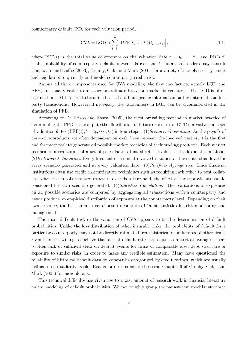
Figure 1: The probability of default p(t, T ) (solid) and p(t, T ) (dashed) as a function of Vt.

We show through a numerical example that the probability of default p(t, T ) is indeed signifi-

cantly higher than p(t, T ). The parameters are taken from the example in Crosbie and Bohn (2003,

page 18) where µ = 0.07, σV = 0.0961, D = 10, T − t = 1. Figure 1 shows that p(t, T ) has a

heavier tail than that of p(t, T ), as the asset value Vt increases from 11 to 13 and consequently the

distance-to-default rises from 1.67 to 3.41. Using the particular example given Crosbie and Bohn

(2003, page 18), when the distance-to-default defined in (2.7) is 3.0, the asset value is roughly

8

12.5116. The prediction from p(t, T ) is 34 basis points whereas that from p(t, T ) is only 13 basis

points.

(2) In the same spirit, the payoff of a European call option overestimates the equity value by

including the cases where the asset values drop below debt value then rise above the debt value at

the end of the prediction period. Thus the valuation of the firm’s equity that is consistent with the

model assumptions should be given by

Et := EQt

[e−r(T−t)(VT −D)+I

(inf

t≤s≤TVs ≥ D

)], (2.8)

which is the price of a down-and-out barrier option. It is also known from Bjork (2004, Proposition

18.8) that

Et =W (Vt)−(D

Vt

)2r/σ2−1

W (D2

Vt).

One should be aware that Et depends on the time until maturity T − t as embedded in W and thus

we shall write Et(s) as a function of the time until maturity s when necessary.

3 Modeling CVA with Downgrade Trigger

We are interested in the valuation of CVA with an additional provision termed downgrade-triggered

termination clause, which has been increasingly common in credit risk management. The downgrade

trigger refers to a credit rating level which is below the initial rating of the counter-party by a

nationally recognized rating agency at the time of inception. In the event that the rating of the

counter-party is downgraded to or below the trigger level prior to maturity, the investor closes off

its position with the counter-party, thereby preventing future losses due to continued worsening of

its credit quality. However, the investor is not entirely immune from potential losses. For example,

if the counter-party defaults immediately after the rating drops below the trigger level, the investor

still experiences a loss due to the counter-party default. Thus the key difference in modeling the

CVA with and without downgrade trigger lies in the measure of the “unprotected” portion of

loss due to the downgrade trigger being inactive prior to default. For brevity, we shall call the

probability of default without a proceeding downgrade below downgrade trigger by the probability

of jump-to-default.

Although there are a variety of models in finance literature for modeling downgrade transitions,

we intend to keep the structure of the KMV-Merton model and seek for a relatively simple extension

for the following reasons. (1) Jump-diffusion structural models have been extensively studied in

finance literature. There are well developed statistical techniques for model calibration. (2) The

KMV model utilizes both market information (stock prices) as well as accounting information (book

value of liability), which means the results can be easily adapted as an interpolation tool for the

pricing of CVA based on known values of CVA with comparable information.

However, it is difficult to use the KMV-Merton model directly for the CVA with downgrade

trigger due to the fact that the geometric Brownian motion does not move fast enough over a short

9

period of time to capture sudden changes in market value, which are the primary triggering events

of a downgrade clause. Hence we introduce a well-known jump-diffusion model proposed by Kou

(2002), Kou and Wang (2003), which can be traced back to Merton (1976) with similar structure.

We assume that the market value of asset follows a jump-diffusion process given by

dVt = Vt− (ν dt+ σ dWt + dZt) , Zt =

Nt∑i=1

(Ui − 1), (3.1)

where Nt, t ≥ 0 is a Poisson process with intensity rate λ independent of W and Ui, i ∈ N is

a sequence of independent and identically distributed non-negative random variables with Ui − 1

representing percentage change caused by the ith jump in the process. Furthermore, we assume

that Yi = lnUi has a bilateral exponential distribution with the density

f(y) = pη1e−η1yIy≥0 + qη2e

η2yIy<0, η1 > 1, η2 > 0, (3.2)

where p, q ≥ 0, p+ q = 1, representing the probabilities of incurring upward and downward jumps.

We shall also denote its distribution function by F . It is known from Ito’s formula that

VT = Vt exp

(ν − 1

2σ2)(T − t) + σWT−t +

NT−t∑k=1

Yk

.

We introduce the notation to formulate the valuation of the CVA with a downgrade trigger.

Consider the market value of assets of the counter-party is driven by the process V = Vt, t ≥ 0defined by the SDE (3.1) on a probability space (Ω,F ,P) with the filtration Ft, t ≥ 0 satisfying

the usual conditions. Denote by A = At, t ≥ 0 the evaluation of net present values of future

cash flows between two parties from the perspective of an investor, which is assumed to be modeled

deterministically in this paper. However, the following analysis does not exclude the possibility that

A is modeled by an independent stochastic process adapted to the filtration Ft, t ≥ 0. In other

words, the process A represents the potential future exposure (PFE) of an OTC transaction between

two counter-parties. Let B be the level of asset value corresponding to the downgrade trigger, T

be the time of maturity of the contract, l be the ratio of loss given default upon the default of the

counter-party. Thus the time of default of the counter-party is given by τD = infs : Vt+s < Dand the first time that the credit rating of a counter-party reaches the downgrade trigger is given by

τB = infs : Vt+s < B where B > D. As hinted in Crosbie and Bohn (2003), one could establish a

mapping between the Vt (or equivalently DD given µ and σV ) and the letter-based credit ratings.

Consequently, one could also use the same mapping to determine the implied distance-to-default

and the corresponding market value B of asset leading to a downgrade.

Hence the primary task of this paper is to provide an efficient and accurate algorithm to compute

the following probabilities of default within a prediction horizon T − t:

1. Probability of default: PτD < T − t

2. Probability of jump-to-default: PτB < T − t, τB = τD.

10

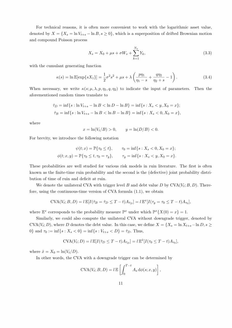
For technical reasons, it is often more convenient to work with the logarithmic asset value,

denoted by X = Xs = lnVt+s − lnB, s ≥ 0, which is a superposition of drifted Brownian motion

and compound Poisson process

Xs = X0 + µs+ σWs +

Ns∑k=1

Yk, (3.3)

with the cumulant generating function

κ(s) = lnE[expsX1] =1

2σ2s2 + µs+ λ

(pη1η1 − s

+qη2η2 + s

− 1

). (3.4)

When necessary, we write κ(s;µ, λ, p, η1, q, η2) to indicate the input of parameters. Then the

aforementioned random times translate to

τD = infs : lnVt+s − lnB < lnD − lnB = infs : Xs < y,X0 = x;

τB = infs : lnVt+s − lnB < lnB − lnB = infs : Xs < 0, X0 = x,

where

x = ln(Vt/B) > 0, y = ln(D/B) < 0.

For brevity, we introduce the following notation

ψ(t;x) = Pτ0 ≤ t, τ0 = infs : Xs < 0, X0 = x;

ϕ(t;x, y) = Pτ0 ≤ t, τ0 = τy, τy = infs : Xs < y,X0 = x.

These probabilities are well studied for various risk models in ruin literature. The first is often

known as the finite-time ruin probability and the second is the (defective) joint probability distri-

bution of time of ruin and deficit at ruin.

We denote the unilateral CVA with trigger level B and debt value D by CVA(Vt;B,D). There-

fore, using the continuous-time version of CVA formula (1.1), we obtain

CVA(Vt;B,D) = lE[I(τB = τD ≤ T − t)AτD ] = lEx[I(τy = τ0 ≤ T − t)Aτ0 ],

where Ex corresponds to the probability measure Px under which PxX(0) = x = 1.

Similarly, we could also compute the unilateral CVA without downgrade trigger, denoted by

CVA(Vt;D), where D denotes the debt value. In this case, we define X = Xs = lnXt+s− lnD, s ≥0 and τ0 := infs : Xs < 0 = infs : Vt+s < D = τD. Thus,

CVA(Vt;D) = lE[I(τD ≤ T − t)AτD ] = lEx[I(τ0 ≤ T − t)Aτ0 ],

where x = X0 = ln(Vt/D).

In other words, the CVA with a downgrade trigger can be determined by

CVA(Vt;B,D) = lE[∫ T−t

0As dϕ(s;x, y)

],

11

whereas the CVA without a downgrade trigger can be written as

CVA(Vt;D) = lE[∫ T−t

0As dψ(s; x)

].

In the next section, we shall first use a ruin theoretic technique to find explicit expressions for the

Laplace-Stieltjes transforms for each fixed x > 0 and y < 0

ϕ(δ;x, y) =

∫ ∞

0e−δs dϕ(s;x, y) = Ex[e−δτ0I(Xτ0 < y, τ0 <∞)], δ ≥ 0, (3.5)

ψ(δ; x) =

∫ ∞

0e−δs dψ(s; x) = Ex[e−δτ0I(τ0 <∞)], δ ≥ 0. (3.6)

Note that ϕ and ψ can be also viewed as the Laplace transform of the density of the time of default

τ0 and that of the time of jump-to-default τ0I(τ0 = τy).

4 Analytic Solution to Laplace Transforms

4.1 Probabilities of Default

We provide an analytic solution to the Laplace-Stieltjes transform using techniques from ruin theory.

Over the past decades, there has been development of systematic tools for analyzing ruin-related

quantities. Most notable is the expected discounted penalty function introduced by Gerber and Shiu

(1998), which characterizes the joint distribution of the time of default, the surplus immediately

prior to ruin and the deficit at ruin. An extension of this function which proves to be convenient

in our discussion is the expected present value of operating costs up to ruin, defined as

H(x) := Ex

[∫ τ0

0e−δtl(Xt) dt

], x ≥ 0, (4.1)

where the function l represents the running cost of a business modeled by the risk process X

and the constant δ is interpreted as the force of interest for discounting. Introduced in Cai et al.

(2009), the function is known to encompass a variety of ruin-related quantities such as the expected

discounted penalty function, aggregate claims and accumulated utilities up to ruin, etc. Although

not immediately evident, simple proofs can be found in Cai et al. (2009) and Feng (2011) that

ϕ(δ;x, y) is a special case of H with the cost function l(x) = λF (y − x) and so is ψ(δ;x) with

l(x) = λF (−x)+∆(x) where ∆ is the Dirac delta function that assigns mass one to the point zero,

and F is the distribution function of the density (3.2).

Theorem 4.1. The Laplace transforms defined in (3.5) and (3.6) with δ > 0 are given by

ϕ(δ;x, y) =(η2 + γ1)(η2 + γ2)e

η2y

η2(γ2 − γ1)[eγ1x − eγ2x], x ≥ 0, y < 0, (4.2)

ψ(δ;x) =γ2(η2 + γ1)

η2(γ2 − γ1)eγ1x − γ1(η2 + γ2)

η2(γ2 − γ1)eγ2x, x ≥ 0, (4.3)

where γ1 = γ1(δ) and γ2 = γ2(δ) are the only two negative roots of κ(s) = δ.

12

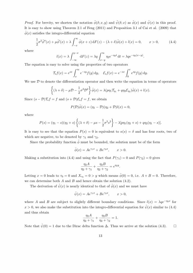
Proof. For brevity, we shorten the notation ϕ(δ;x, y) and ψ(δ;x) as ϕ(x) and ψ(x) in this proof.

It is easy to show using Theorem 2.1 of Feng (2011) and Proposition 3.1 of Cai et al. (2009) that

ϕ(x) satisfies the integro-differential equation

1

2σ2ϕ′′(x) + µϕ′(x) + λ

∫ ∞

−xϕ(x+ z) dF (z)− (λ+ δ)ϕ(x) + l(x) = 0, x > 0, (4.4)

where

l(x) = λ

∫ y−x

−∞dF (z) = λq

∫ ∞

x−yη2e

−η2t dt = λqe−η2(x−y).

The equation is easy to solve using the properties of two operators

Tsf(x) = esx∫ ∞

xe−syf(y) dy, Esf(x) = e−sx

∫ x

0esyf(y) dy.

We use D to denote the differentiation operator and then write the equation in terms of operators(λ+ δ)− µD − 1

2σ2D2

ϕ(x) = λ(pη1Tη1 + qη2Eη2)ϕ(x) + l(x).

Since (s−D)Tsf = f and (s+D)Esf = f , we obtain

P (D)ϕ(x) = (η1 −D)(η2 +D)l(x) = 0,

where

P (s) = (η1 − s)(η2 + s)

(λ+ δ)− µs− 1

2σ2s2

− λ[pη1(η2 + s) + qη2(η1 − s)].

It is easy to see that the equation P (s) = 0 is equivalent to κ(s) = δ and has four roots, two of

which are negative, to be denoted by γ1 and γ2.

Since the probability function ϕ must be bounded, the solution must be of the form

ϕ(x) = Aeγ1x +Beγ2x, x > 0.

Making a substitution into (4.4) and using the fact that P (γ1) = 0 and P (γ2) = 0 gives

η2A

η2 + γ1+

η2B

η2 + γ2= eη2y.

Letting x = 0 leads to τ0 = 0 and Xτ0 = 0 > y which means ϕ(0) = 0, i.e. A+ B = 0. Therefore,

we can determine both A and B and hence obtain the solution (4.2).

The derivation of ψ(x) is nearly identical to that of ϕ(x) and we must have

ψ(x) = Aeγ1x +Beγ2x, x > 0,

where A and B are subject to slightly different boundary conditions. Since l(x) = λqe−η2x for

x > 0, we also make the substitution into the integro-differential equation for ψ(x) similar to (4.4)

and thus obtainη2A

η2 + γ1+

η2B

η2 + γ2= 1.

Note that ψ(0) = 1 due to the Dirac delta function ∆. Thus we arrive at the solution (4.3).

13

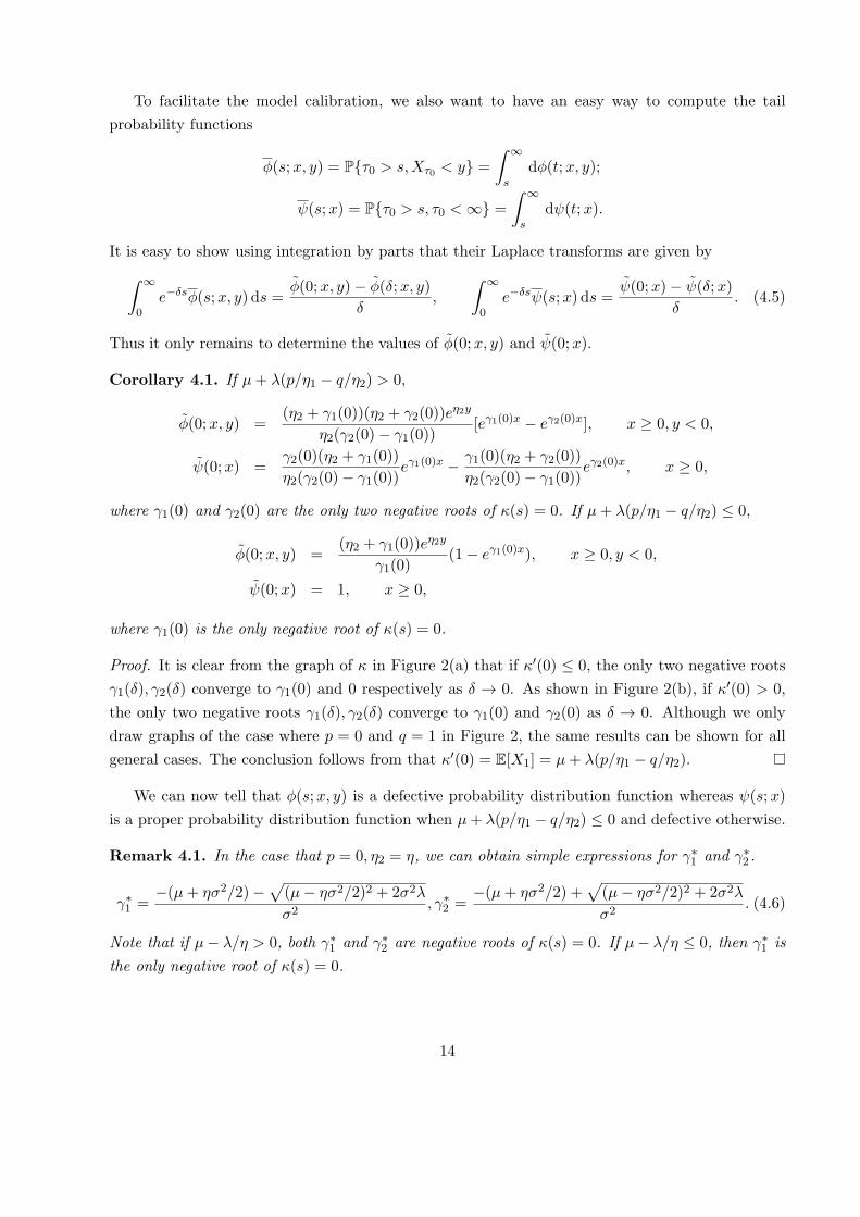
To facilitate the model calibration, we also want to have an easy way to compute the tail

probability functions

ϕ(s;x, y) = Pτ0 > s,Xτ0 < y =

∫ ∞

sdϕ(t;x, y);

ψ(s;x) = Pτ0 > s, τ0 <∞ =

∫ ∞

sdψ(t;x).

It is easy to show using integration by parts that their Laplace transforms are given by∫ ∞

0e−δsϕ(s;x, y) ds =

ϕ(0;x, y)− ϕ(δ;x, y)

δ,

∫ ∞

0e−δsψ(s;x) ds =

ψ(0;x)− ψ(δ;x)

δ. (4.5)

Thus it only remains to determine the values of ϕ(0;x, y) and ψ(0;x).

Corollary 4.1. If µ+ λ(p/η1 − q/η2) > 0,

ϕ(0;x, y) =(η2 + γ1(0))(η2 + γ2(0))e

η2y

η2(γ2(0)− γ1(0))[eγ1(0)x − eγ2(0)x], x ≥ 0, y < 0,

ψ(0;x) =γ2(0)(η2 + γ1(0))

η2(γ2(0)− γ1(0))eγ1(0)x − γ1(0)(η2 + γ2(0))

η2(γ2(0)− γ1(0))eγ2(0)x, x ≥ 0,

where γ1(0) and γ2(0) are the only two negative roots of κ(s) = 0. If µ+ λ(p/η1 − q/η2) ≤ 0,

ϕ(0;x, y) =(η2 + γ1(0))e

η2y

γ1(0)(1− eγ1(0)x), x ≥ 0, y < 0,

ψ(0;x) = 1, x ≥ 0,

where γ1(0) is the only negative root of κ(s) = 0.

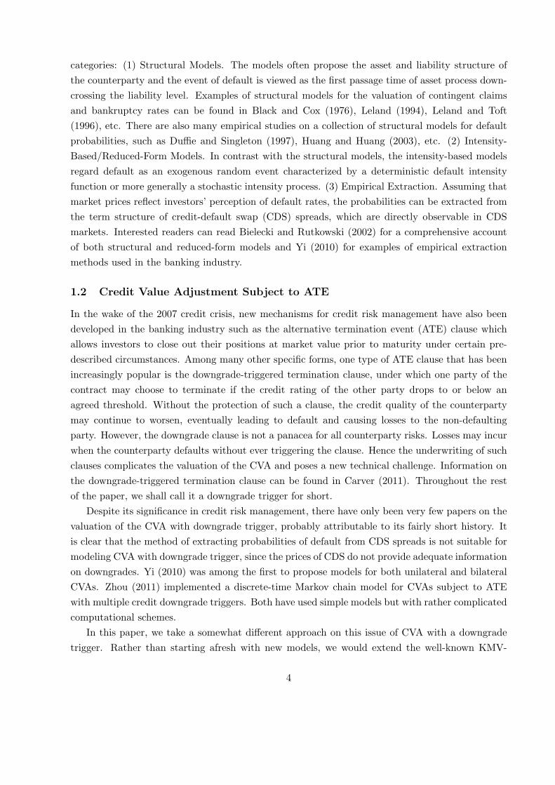
Proof. It is clear from the graph of κ in Figure 2(a) that if κ′(0) ≤ 0, the only two negative roots

γ1(δ), γ2(δ) converge to γ1(0) and 0 respectively as δ → 0. As shown in Figure 2(b), if κ′(0) > 0,

the only two negative roots γ1(δ), γ2(δ) converge to γ1(0) and γ2(0) as δ → 0. Although we only

draw graphs of the case where p = 0 and q = 1 in Figure 2, the same results can be shown for all

general cases. The conclusion follows from that κ′(0) = E[X1] = µ+ λ(p/η1 − q/η2).

We can now tell that ϕ(s;x, y) is a defective probability distribution function whereas ψ(s;x)

is a proper probability distribution function when µ+ λ(p/η1 − q/η2) ≤ 0 and defective otherwise.

Remark 4.1. In the case that p = 0, η2 = η, we can obtain simple expressions for γ∗1 and γ∗2 .

γ∗1 =−(µ+ ησ2/2)−

√(µ− ησ2/2)2 + 2σ2λ

σ2, γ∗2 =

−(µ+ ησ2/2) +√

(µ− ησ2/2)2 + 2σ2λ

σ2. (4.6)

Note that if µ− λ/η > 0, both γ∗1 and γ∗2 are negative roots of κ(s) = 0. If µ− λ/η ≤ 0, then γ∗1 is

the only negative root of κ(s) = 0.

14

4.2 Valuation of Equity

In the framework of the KMV-Merton model, the market value of the firm is not observable. The

parameters are usually estimated indirectly through the observable data on equity values viewed as

an option on firm value. The European call option has been used due to its analytical tractability.

As we have explained earlier, the valuation of equity as a down-and-out barrier option appears to

be more consistent with the purpose of forecasting the probability of default over a period of time.

The pricing of barrier option under the double exponential jump-diffusion model has been

developed in Kou and Wang (2003) with an example of up-and-in call option. Following the same

technique as shown in Kou and Wang (2003), we can easily show that the Laplace transform of the

down-and-out call option (2.8) follows immediately from the formula for the probability of default.

It is known that in general jump-diffusion models do not lead to a unique risk neutral mea-

sure. Kou (2002) employed a rational expectation equilibrium argument to derive a particular risk

neutral measure. In the KMV-Merton model, the parameters are estimated from observed data on

“options” and hence we do not need to specify the particular choices of measure. Under any risk

neutral measure, the market value of assets is given by

VT = Vt exp XT−t , where Xs = r∗s+ σWs +

Ns∑k=1

Yk,

where r is the risk-free force of interest earned in a bank account and

r∗ := r − 1

2σ2 − λζ, ζ :=

pη1η1 − 1

+qη2η2 + 1

− 1.

Theorem 4.2. If the asset value of the firm is driven by the jump-diffusion process (3.1), the

Laplace transform of the asset value Et defined by (2.8) is given by

E(δ) :=

∫ ∞

0e−δsEt(s) ds

=Vtδ

1− γ2(η2 + γ1)

η2(γ2 − γ1)

(VtD

)γ1

+γ1(η2 + γ2)

η2(γ2 − γ1)

(VtD

)γ2

− D

δ + r

1− γ2(η2 + γ1)

η2(γ2 − γ1)

(VtD

)γ1

+γ1(η2 + γ2)

η2(γ2 − γ1)

(VtD

)γ2

,

where γ1 and γ2 are the two negative roots of κ(s; r∗, λ, p, η1, q, η2) = δ, γ1 and γ2 are the two

negative roots of κ(s; r∗, λ, p, η1, q, η2) = δ + r, and

p =pη1

(1 + ζ)(η1 − 1), q =

qη2(1 + ζ)(η2 + 1)

, λ = λ(1 + ζ), η1 = η1 − 1, η2 = η2 + 1. (4.7)

Proof. We apply the usual technique of a change of measure using the Esscher transform

dQdQ

∣∣∣∣∣FT

= e−r(T−t)VTVt

= expXT−t − r(T − t).

15

Interested readers may read Gerber and Shiu (1994) for details on the Esscher transform. It is

easy to show that under Qt, the logarithmic market value process X is still a double exponential

jump-diffusion process but with a different set of parameters given in (4.7). The risk free force of

interest r∗ and volatility coefficient σ do not change under this measure.

It follows from the definition (2.8) that

Et(T − t) = EQt [e

−r(T−t)VT I(VT ≥ D, τD > T − t)]−De−r(T−t)EQt [I(VT ≥ D, τD > T − t)]

= VtEQt [I(τD > T − t)]−De−r(T−t)EQ

t [I(VT ≥ D, τD > T − t)].

For notational brevity, we introduce Xs = lnVt+s− lnD for all s ≥ 0 and hence X0 = ln(Vt/D) > 0.

Similarly we must have

τ0 = infs ≥ 0 : Xs ≤ 0 = τD = infs ≥ 0 : Vt+s ≤ D.

Therefore,

Et(s) = VtQtτ0 > s −De−rsQtτ0 > s

= Vt[1− Qtτ0 ≤ s]−De−rs[1−Qtτ0 ≤ s].

Taking the Laplace transform gives

E(δ) =Vtδ[1− ψ1(δ; ln(Vt/D))]− D

δ + r[1− ψ2(δ + r; ln(Vt/D))],

where ψ1(δ, x) is the Laplace transform of the probability density function of the time of default

under measure Qt and ψ2(δ, x) is that under measure Qt. Hence the two are of the same form but

with different sets of parameters.

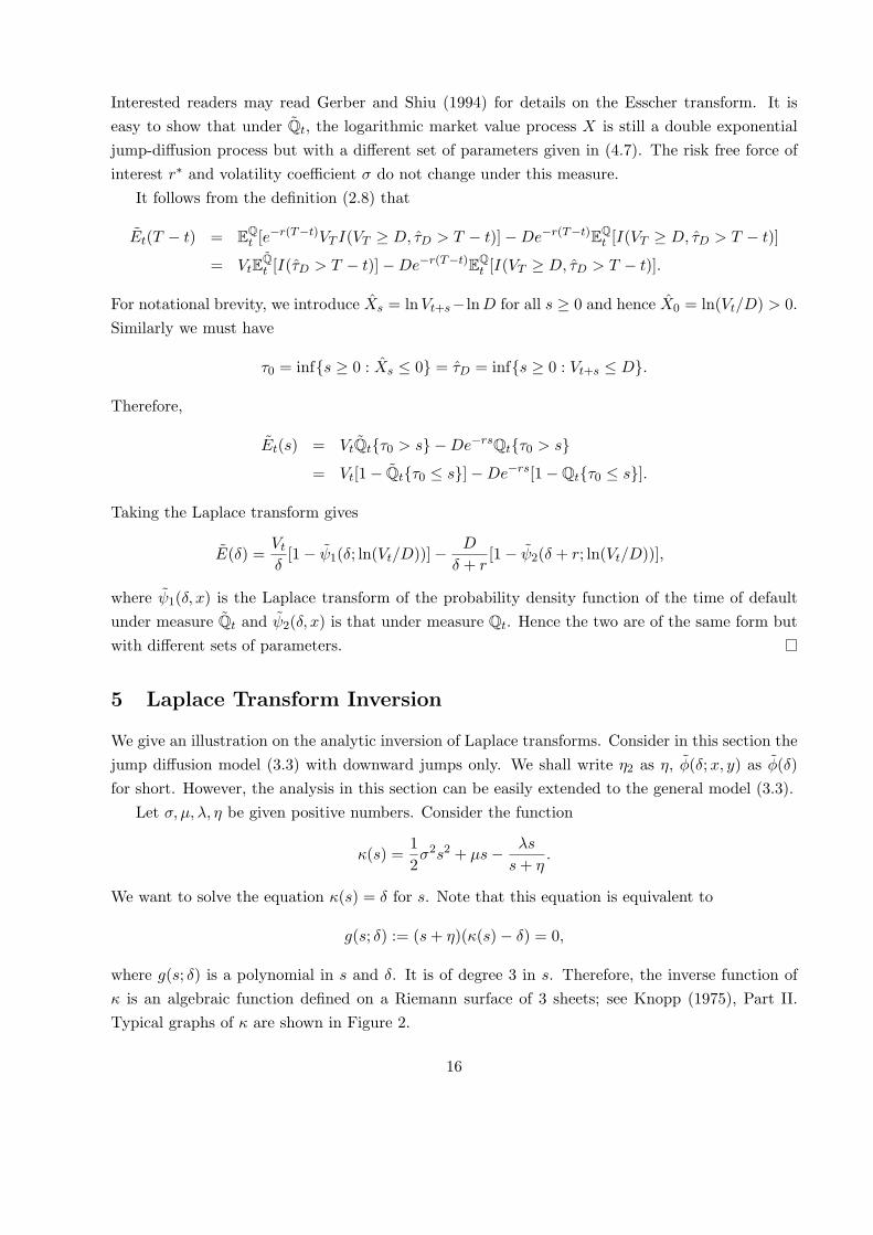
5 Laplace Transform Inversion

We give an illustration on the analytic inversion of Laplace transforms. Consider in this section the

jump diffusion model (3.3) with downward jumps only. We shall write η2 as η, ϕ(δ;x, y) as ϕ(δ)

for short. However, the analysis in this section can be easily extended to the general model (3.3).

Let σ, µ, λ, η be given positive numbers. Consider the function

κ(s) =1

2σ2s2 + µs− λs

s+ η.

We want to solve the equation κ(s) = δ for s. Note that this equation is equivalent to

g(s; δ) := (s+ η)(κ(s)− δ) = 0,

where g(s; δ) is a polynomial in s and δ. It is of degree 3 in s. Therefore, the inverse function of

κ is an algebraic function defined on a Riemann surface of 3 sheets; see Knopp (1975), Part II.

Typical graphs of κ are shown in Figure 2.

16

s

–2

–1

1

2

3

–6 –4 –2 2 4

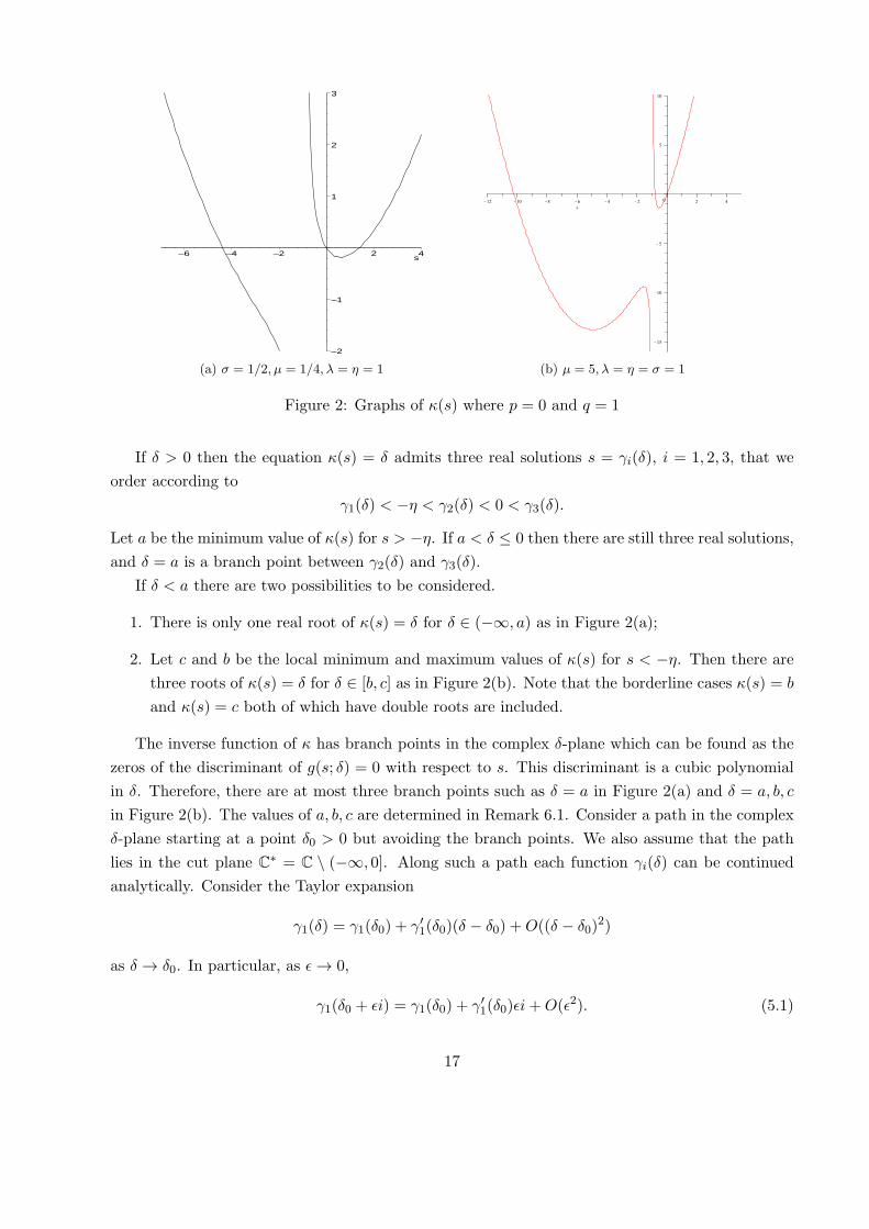
(a) σ = 1/2, µ = 1/4, λ = η = 1 (b) µ = 5, λ = η = σ = 1

Figure 2: Graphs of κ(s) where p = 0 and q = 1

If δ > 0 then the equation κ(s) = δ admits three real solutions s = γi(δ), i = 1, 2, 3, that we

order according to

γ1(δ) < −η < γ2(δ) < 0 < γ3(δ).

Let a be the minimum value of κ(s) for s > −η. If a < δ ≤ 0 then there are still three real solutions,

and δ = a is a branch point between γ2(δ) and γ3(δ).

If δ < a there are two possibilities to be considered.

1. There is only one real root of κ(s) = δ for δ ∈ (−∞, a) as in Figure 2(a);

2. Let c and b be the local minimum and maximum values of κ(s) for s < −η. Then there are

three roots of κ(s) = δ for δ ∈ [b, c] as in Figure 2(b). Note that the borderline cases κ(s) = b

and κ(s) = c both of which have double roots are included.

The inverse function of κ has branch points in the complex δ-plane which can be found as the

zeros of the discriminant of g(s; δ) = 0 with respect to s. This discriminant is a cubic polynomial

in δ. Therefore, there are at most three branch points such as δ = a in Figure 2(a) and δ = a, b, c

in Figure 2(b). The values of a, b, c are determined in Remark 6.1. Consider a path in the complex

δ-plane starting at a point δ0 > 0 but avoiding the branch points. We also assume that the path

lies in the cut plane C∗ = C \ (−∞, 0]. Along such a path each function γi(δ) can be continued

analytically. Consider the Taylor expansion

γ1(δ) = γ1(δ0) + γ′1(δ0)(δ − δ0) +O((δ − δ0)2)

as δ → δ0. In particular, as ϵ→ 0,

γ1(δ0 + ϵi) = γ1(δ0) + γ′1(δ0)ϵi+O(ϵ2). (5.1)

17

Since γ1(δ) is a decreasing function of δ > 02 (as is evident from the fact that s = γ1(δ) < −η is the

only solution of κ(s) = δ > 0), we have γ′1(δ0) < 0. Therefore, (5.1) shows that, for ϵ sufficiently

close to 0,

ϵℑγ1(δ0 + ϵi) < 0.

It is obvious that solutions s of κ(s) = δ are never real if ℑδ = 0. Therefore, by the intermediate

value theorem, the sign of the imaginary part of the analytic continuation of γ1(δ) is opposite to

that of ℑδ whenever ℑδ = 0. The same argument holds with γ2(δ) in place of γ1(δ). Analogously,

γ3(δ) is an increasing function of δ > 0 and so its analytic continuation has an imaginary part of the

same sign as ℑδ = 0. Therefore, s = γ3(δ) is the only solution of g(s; δ) = 0 whose imaginary part

has the same sign as that of ℑδ = 0. This shows that γ3(δ) cannot have branch points in C∗, and

so, by the monodromy theorem, γ3(δ) is an analytic function on C∗. Moreover, while γ1(δ), γ2(δ)

may have branch points in C∗, the unordered pair γ1(δ), γ2(δ) is well-defined for δ ∈ C∗. This

pair consists of the two solutions of g(s; δ) = 0 whose imaginary parts have signs opposite to that

of ℑδ = 0.

For δ > 0 we consider the function

ϕ(δ) =(γ1(δ) + η)(γ2(δ) + η)eyη

η(γ2(δ)− γ1(δ))

(exγ1(δ) − exγ2(δ)

), (5.2)

where x > 0 and y are given constant. This function has the form

ϕ(δ) = K(γ1(δ), γ2(δ)),

where K is an analytic function on C2 which is symmetric, that is, F (u, v) = F (v, u). Therefore,

by analytic continuation, ϕ(δ) becomes an analytic function in C∗ (the branch points of the inverse

function of κ lying in C∗ are removable singularities of ϕ.) We can actually compute ϕ(δ) as

follows. For given δ ∈ C with ℑδ = 0, we compute the zeros of g(s; δ) = 0. These zeros can be

found numerically or using Cardano’s formula for the solution of the cubic equation. Two of them

have imaginary part opposite to that of ℑδ. We use these solutions as γ1 and γ2 in (5.2). We note

that the calculation of ϕ(δ) for complex values of δ is required for several of the numerical inversion

methods of the Laplace transform of ϕ(δ); see Abate and Whitt (1995).

Since we know that ϕ(δ) is analytic on C∗ we can find the inverse Laplace transform f(t) of

ϕ(δ) in a more convenient way as follows. We start with the well known formula

f(t) =1

2πi

∫ i∞

−i∞eδtϕ(δ) dδ. (5.3)

2To prove this directly one needs to show that κ(s) is decreasing for s < −η as long as κ(s) > 0. We assume that

s < −η < 0 and κ(s) > 0. Then 12σ2s+ µ− λ

s+η< 0, so µ < λ

s+η− 1

2σ2s. Using this inequality we obtain

κ′(s) = σ2s+ µ− λη

(s+ η)2<

1

2σ2s+

λs

(s+ η)2< 0.

18

In the integral (5.3) we deform the path of integration towards the negative δ-axis as described in

Doetsch (1974, Section 25, page 161). We obtain that

f(t) =1

2πi

∫Ceδtϕ(δ) dδ, (5.4)

where C is the path coming from −∞ following the lower boundary of the cut (−∞, 0] until 0 and

then returning to −∞ along the upper boundary of the cut. We can show that δϕ(δ) is a bounded

function on C∗ (the proof is omitted). Therefore, Doetsch (1974, Theorem 25.1, page 162) justifies

the step from (5.3) to (5.4). If ϕ(δ ± i0) denote the values of ϕ on the cut for δ < 0 then ϕ(δ + i0)

is conjugate to ϕ(δ − i0). Therefore, we can simplify (5.4) to

f(t) =1

π

∫ 0

−∞eδtℑϕ(δ − i0) dδ. (5.5)

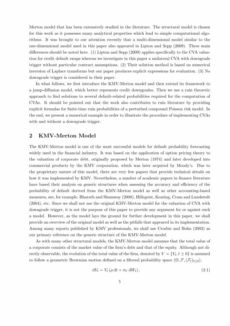
The function ℑϕ(δ− i0) can be computed for given δ < 0 as follows. If the equation g(s; δ) = 0 has

only real zeros (as happens for a ≤ δ < 0) then ℑϕ(δ− i0) = 0 and there is nothing to compute. If

g(s, δ) = 0 has one real zero (which is negative) and two complex conjugate zeros then we evaluate

ϕ(δ − i0) by using (5.2) with γ1 and γ2 replaced by the negative zero and the zero with positive

imaginary part. A typical graph of ℑϕ(δ − i0) is shown in Figure 3.

–0.2

0

0.2

0.4

0.6

0.8

1

1.2

1.4

1.6

–8 –7 –6 –5 –4 –3 –2 –1

Figure 3: Graph of ℑϕ(δ − i0) for σ = 12 , µ = 1

4 , λ = η = 1

Numerical experiments show that the computation of the function f(t) based on formula (5.5)

is very effective especially if t is large. A similar analysis can be carried out for ψ(δ;x) as well as

the Laplace transforms of ψ and ϕ defined in (4.5).

6 Finite-time Ruin Probability

In this section, we divert to show a by-product of our analysis on the inverse Laplace transform.

In recent ruin literature, explicit solutions have been found to finite-time ruin probabilities in a

19

variety of risk models, such as Asmussen (1984), Dickson and Willmot (2005), etc. for compound

Poisson risk models; Dickson and Li (2010), Borovkov and Dickson (2008), Landriault et al. (2011),

etc. for the Sparre Andersen risk models. The list is far from being comprehensive. However, it

appears that finite-time ruin probabilities were not previously known for jump-diffusion models

such as (3.3). We shall now provide a new addition to the list of explicit solutions in the framework

of (3.3) with downward exponential jumps only.

Theorem 6.1. The finite-time ruin probability is given by

ψ(t;x) = ψ(0;x)

+1

π

∫S

s1(s1 + η)zewx cos(zx)− (s1 + η)zes1x − [(η + w)(w − s1) + z2]ewx sin(zx)eδt

δη[(w − s1)2 + z2]dδ,

(6.1)

where S = δ < 0 : D(δ) > 0 and all other expressions are real and given by

s1 = u+ v − A

3, w = −1

2(u+ v)− A

3, z =

√3

2(u− v), A =

2µ+ ησ2

σ2, B =

2(ηµ− λ− δ)

σ2, C =

−2ηδ

σ2,

D(δ) =(q2

)2+(p3

)3, u = 3

√−q2+√D(δ), v = 3

√−q2−√D(δ), p = B − 1

3A2, q =

2

27A3 − 1

3AB + C.

Proof. We can compute ψ(t;x) by ψ(t;x) = ψ(0;x)− ψ(t;x). The first term ψ(0;x) is determined

in Corollary 4.1. In view of (4.5), the second term ψ(t;x) can be found by inverting the Laplace

transform

ψ(t;x) =1

π

∫ 0

−∞ℑ

(ψ(0;x)− ψ(δ;x)

δ

)eδt dδ = − 1

π

∫ 0

−∞ℑ(ψ(δ;x)

) 1

δeδt dδ.

Thus the proof is completed when the imaginary part of ψ(δ;x) is identified. To this end, we

introduce Cardano’s formula for cubic roots. Since γ1(δ) and γ2(δ) are both solutions to the cubic

equation αs3 + βs2 + θs+ ζ = 0, where α = σ2/2, β = µ+ ησ2/2, θ = ηµ− λ− δ, ζ = −ηδ, we can

work with the equivalent cubic equation s3+As2+Bs+C = 0 and then set s = y−A/3 to obtain

y3 + py + q = 0 with the discriminant D(δ). If D(δ) < 0 there are three real roots and if D(δ) > 0

there is one real root and a pair of complex conjugate roots. If D(δ) < 0, then ψ(δ − i0) is real

so ℑψ(δ − i0) = 0 and we do not have to compute anything. If D(δ) > 0 then we introduce real

numbers u and v. Thus the three roots are

y1 = u+ v, y2 = −1

2(u+ v) + i

√3

2(u− v), y3 = −1

2(u+ v)− i

√3

2(u− v).

The solutions of the original cubic equation are si = yi − a/3. It is clear that s1 is real and s2, s3

are conjugate with ℑs2 > 0. Therefore, we substitute the two expressions s1 for γ1(δ) and s2 for

γ2(δ) into (4.3) for ψ(δ − i0) with negative δ. We can now calculate the imaginary part of this

expression since we have formulas for real part and imaginary part of s2 while all other numbers

are real. Knowing that s2 = w + iz, we obtain the formula (6.1) after algebraic simplification.

20

Remark 6.1. The constant ψ(0;x) is given in Corollary 4.1 with the constants in (4.6). The

domain of integration S can be determined easily by either of the following two cases. Note that

for some constants a∗, b∗, c∗, d∗, we can write

D(δ) = a∗δ3 + b∗δ2 + c∗δ + d∗.

These coefficients can be obtained easily using computer algebra systems such as Maple. Similar to

previous proof, we rewrite D(δ) = 0 as δ3+A∗δ2+B∗δ+C∗ = 0 with A∗ = b∗/a∗, B∗ = c∗/a∗, C∗ =

d∗/a∗. By setting δ = t−A∗/3, we obtain the depressed cubic equation

t3 + p∗t+ q∗ = 0, where p∗ = B∗ − 1

3(A∗)2, q∗ =

2

27(A∗)3 − 1

3A∗B∗ + C∗,

which has three zeros

tk = 2

√−p

∗

3cos

(1

3arccos

(3q∗

2p∗

√−3

p∗

)− k

2π

3

), k = 0, 1, 2.

Let D∗ = (q∗/2)2 + (p∗/3)3. If D∗ > 0, then κ(s) = δ has only one real root for δ ∈ (−∞, 0] as

shown in Figure 2(a) and the unique real root a = 3

√−q∗/2 +

√D∗ + 3

√−q∗/2−

√D∗ −A∗/3 and

hence S = (−∞, a). If D∗ ≤ 0, then κ(s) = δ has three real roots for δ ∈ (−∞, 0] as appeared in

Figure 2(b), a = t0 −A∗/3, b = t1 −A∗/3, c = t2 −A∗/3 and S = (−∞, c)∪(b, a).

The formula (6.1) can be viewed as a generalization of the well-known formulas for finite-time

ruin probability in the classical compound Poisson model with exponential claims. See for example,

Ch. V. Prop. 1.3 of Asmussen and Albrecher (2010), Theorem 5.6.4 of Rolski et al. (1998) for

the explicit formulas. Since the classical compound Poisson model can be viewed as the limiting

case of the model (3.3) as σ goes to zero, we give a numerical example in Table 2 to illustrate the

convergence of ψ(t;x) to its counterpart finite-time ruin probability in the classical model, denoted

by ψc(t;x). The values of ψc(t;x) are computed using both (5.6.11) of Rolski et al. (1998) and

Ch.V (1.6) of Asmussen and Albercher (2010).

σ ψ(t;x) ψc(t;x)

0.1 0.2470612116 0.2459378310

0.01 0.2459490849 0.2459378310

0.001 0.2459379434 0.2459378310

0.0001 0.2459378320 0.2459378310

Table 2: Comparison of finite-time ruin probabilities (t = x = µ = λ = η = 1)

We could also reproduce the classical result using the method described in Section 5. In the

classical compound Poisson model, the function κ reduces to

κ(s) = µs− λs

s+ η,

21

where λ, µ, η > 0. Taking the limit of (4.3) as σ goes to zero, the Laplace transform of finite-time

ruin probability is given by

ψc(δ;x) =η + γ2η

eγ2x,

where γ2 is the non-positive root of k(s) = 0. Note that k(s) = 0 is equivalent to

g(s) = µs2 + µηs− λs− δs− δη = 0. (6.2)

Thus,

γ2 =(λ+ δ − µη)−

√(λ+ δ − µη)2 + 4µδη

2µ.

Since the discriminant of (6.2) is given by

∆(δ) = δ2 + 2(λ+ µη)δ + (λ− µη)2,

then γ2 must have a non-zero imaginary part when

δ ∈ S := (−(√λ+

√µη)2,−(

√λ−√

µη)2),

and be real when δ ∈ R\S. Therefore, using the same method as in the proof of Theorem 6.1, we

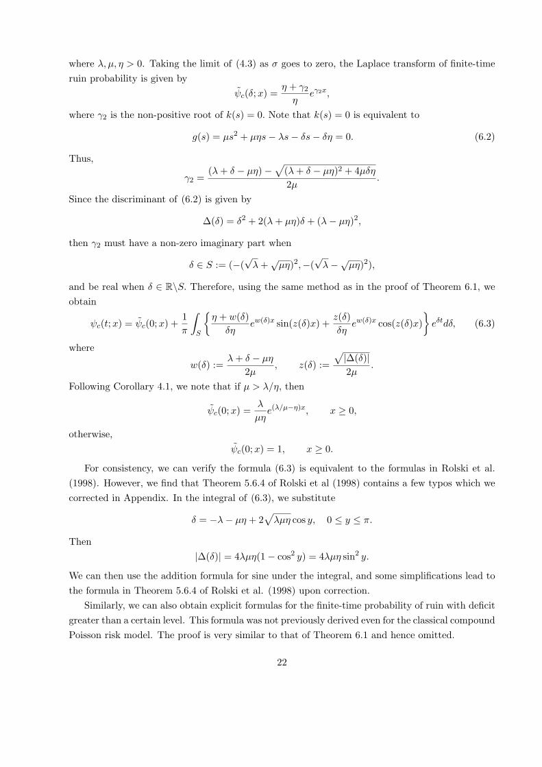
obtain

ψc(t;x) = ψc(0;x) +1

π

∫S

η + w(δ)

δηew(δ)x sin(z(δ)x) +

z(δ)

δηew(δ)x cos(z(δ)x)

eδtdδ, (6.3)

where

w(δ) :=λ+ δ − µη

2µ, z(δ) :=

√|∆(δ)|2µ

.

Following Corollary 4.1, we note that if µ > λ/η, then

ψc(0;x) =λ

µηe(λ/µ−η)x, x ≥ 0,

otherwise,

ψc(0;x) = 1, x ≥ 0.

For consistency, we can verify the formula (6.3) is equivalent to the formulas in Rolski et al.

(1998). However, we find that Theorem 5.6.4 of Rolski et al (1998) contains a few typos which we

corrected in Appendix. In the integral of (6.3), we substitute

δ = −λ− µη + 2√λµη cos y, 0 ≤ y ≤ π.

Then

|∆(δ)| = 4λµη(1− cos2 y) = 4λµη sin2 y.

We can then use the addition formula for sine under the integral, and some simplifications lead to

the formula in Theorem 5.6.4 of Rolski et al. (1998) upon correction.

Similarly, we can also obtain explicit formulas for the finite-time probability of ruin with deficit

greater than a certain level. This formula was not previously derived even for the classical compound

Poisson risk model. The proof is very similar to that of Theorem 6.1 and hence omitted.

22

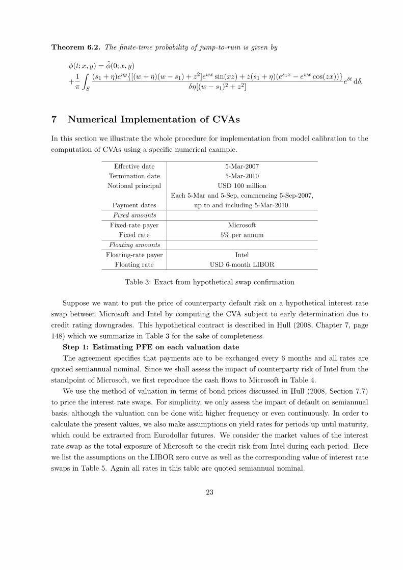
Theorem 6.2. The finite-time probability of jump-to-ruin is given by

ϕ(t;x, y) = ϕ(0;x, y)

+1

π

∫S

(s1 + η)eηy[(w + η)(w − s1) + z2]ewx sin(xz) + z(s1 + η)(es1x − ewx cos(zx))δη[(w − s1)2 + z2]

eδt dδ,

7 Numerical Implementation of CVAs

In this section we illustrate the whole procedure for implementation from model calibration to the

computation of CVAs using a specific numerical example.

Effective date 5-Mar-2007

Termination date 5-Mar-2010

Notional principal USD 100 million

Each 5-Mar and 5-Sep, commencing 5-Sep-2007,

Payment dates up to and including 5-Mar-2010.

Fixed amounts

Fixed-rate payer Microsoft

Fixed rate 5% per annum

Floating amounts

Floating-rate payer Intel

Floating rate USD 6-month LIBOR

Table 3: Exact from hypothetical swap confirmation

Suppose we want to put the price of counterparty default risk on a hypothetical interest rate

swap between Microsoft and Intel by computing the CVA subject to early determination due to

credit rating downgrades. This hypothetical contract is described in Hull (2008, Chapter 7, page

148) which we summarize in Table 3 for the sake of completeness.

Step 1: Estimating PFE on each valuation date

The agreement specifies that payments are to be exchanged every 6 months and all rates are

quoted semiannual nominal. Since we shall assess the impact of counterparty risk of Intel from the

standpoint of Microsoft, we first reproduce the cash flows to Microsoft in Table 4.

We use the method of valuation in terms of bond prices discussed in Hull (2008, Section 7.7)

to price the interest rate swaps. For simplicity, we only assess the impact of default on semiannual

basis, although the valuation can be done with higher frequency or even continuously. In order to

calculate the present values, we also make assumptions on yield rates for periods up until maturity,

which could be extracted from Eurodollar futures. We consider the market values of the interest

rate swap as the total exposure of Microsoft to the credit risk from Intel during each period. Here

we list the assumptions on the LIBOR zero curve as well as the corresponding value of interest rate

swaps in Table 5. Again all rates in this table are quoted semiannual nominal.

23

Date 6m LIBOR (%) Received Paid Net

5-Mar-2007 4.20

5-Sep-2007 4.80 +2.10 −2.50 −0.40

5-Mar-2008 5.30 +2.40 −2.50 −0.10

5-Sep-2008 5.50 +2.65 −2.50 +0.15

5-Mar-2009 5.60 +2.75 −2.50 +0.25

5-Sep-2009 5.90 +2.80 −2.50 +0.45

Table 4: Cash flows to Microsoft

k Date 6m LIBOR 12m LIBOR 18m LIBOR 24m LIBOR 30m LIBOR PFEk

0 5-Mar-2007 4.20 - - - - 0

1 5-Sep-2007 4.80 4.90 5.20 5.30 5.50 0.48525954

2 5-Mar-2008 5.30 5.50 5.80 6.00 - 1.83211570

3 5-Sep-2008 5.50 5.70 5.90 - - 1.264783917

4 5-Mar-2009 5.60 5.90 - - - 0.858142332

5 5-Sep-2009 5.90 - - - - 0.437105391

Table 5: The value of Interest Rate Swap (IRS) to Microsoft

Step 2: Calibrating model parameters for PD

In principle, the calibration of the model (3.3) can be done similarly to that of the KMV-Merton

model. Taking advantage of the well-developed estimation methods described in Section 2, we can

assume that the drift and volatility coefficients are taken from the KMV-Merton model without

jump components. Then the parameters from the jump component, namely λ, p, η1, η2 can be

chosen to adjust the default probabilities. As stated in Crosbie and Bohn (2003), the predictions

on probabilities of default from the geometric Brownian motion are often too low to be credible

for commercial use. With the freedom of extra parameters from the jump component, the model

(3.3) is equipped with additional leverage to match the probabilities of default to an empirical level

within a certain time horizon. This technique known as quantile matching is often used in the

insurance industry for calibrating parameters of asset pricing models. Readers may read Hardy

(2003, Chapter 4) for detailed discussion.

In this numerical example, we assume that the best estimates µ = 0.07 and σ = 0.0961 are

already known from data analysis of Intel’s stock prices using KMV-Merton iterative methods

and the estimated asset value of Intel is Vt = $12.5116 billions and the book value of its liability is

D = $9.0948 billion, which corresponds to the distance-to-default of 4.0 according to (2.7). (Some of

these parameters were quoted from Crosbie and Bohn (2003, page 18) used for an unknown entity.)

Since Crosbie and Bohn (2003) argued that empirical study shows the distance-of-default of four

corresponds to a default rate of around 100 basis points, we want to ensure that the remaining

parameters are chosen so that the one-year probability of default matches the empirical estimate.

In this case we use the model (3.3) with downward jumps only, which represent hazardous

24

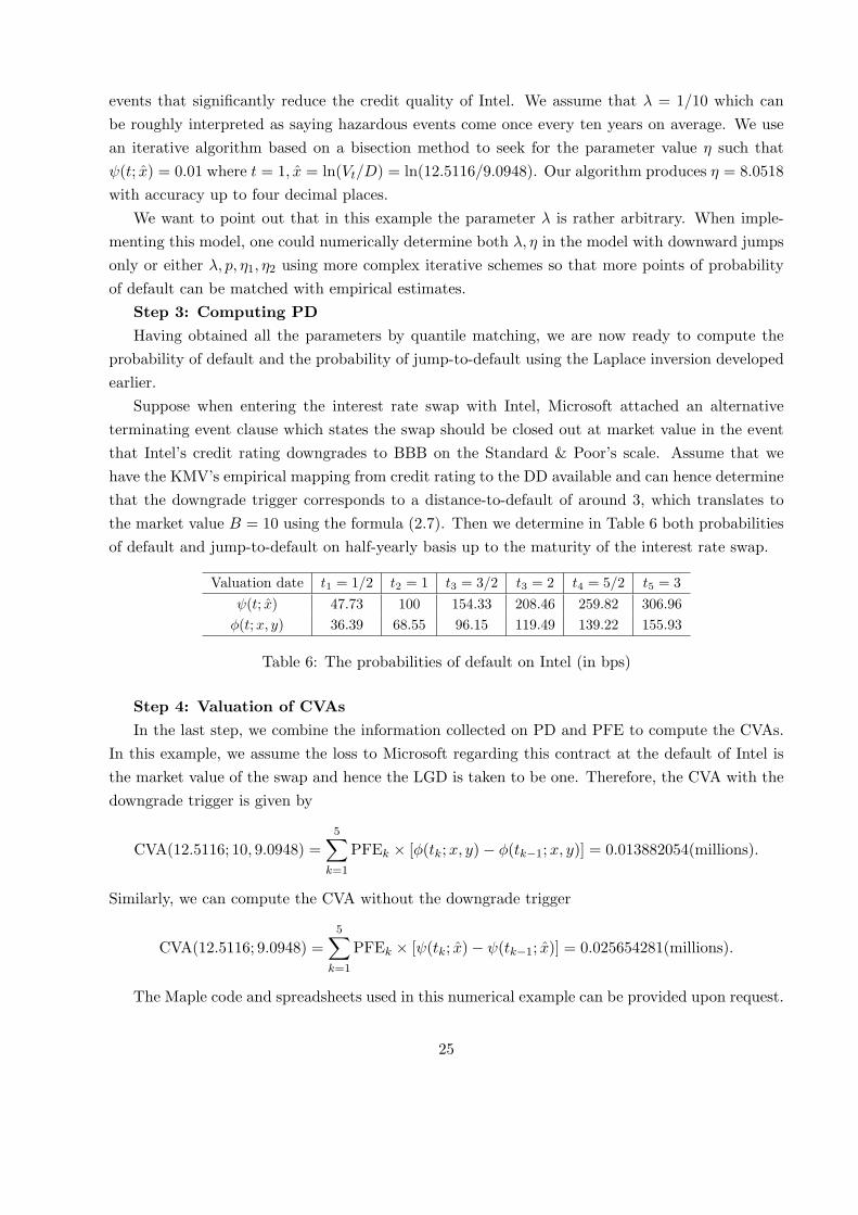
events that significantly reduce the credit quality of Intel. We assume that λ = 1/10 which can

be roughly interpreted as saying hazardous events come once every ten years on average. We use

an iterative algorithm based on a bisection method to seek for the parameter value η such that

ψ(t; x) = 0.01 where t = 1, x = ln(Vt/D) = ln(12.5116/9.0948). Our algorithm produces η = 8.0518

with accuracy up to four decimal places.

We want to point out that in this example the parameter λ is rather arbitrary. When imple-

menting this model, one could numerically determine both λ, η in the model with downward jumps

only or either λ, p, η1, η2 using more complex iterative schemes so that more points of probability

of default can be matched with empirical estimates.

Step 3: Computing PD

Having obtained all the parameters by quantile matching, we are now ready to compute the

probability of default and the probability of jump-to-default using the Laplace inversion developed

earlier.

Suppose when entering the interest rate swap with Intel, Microsoft attached an alternative

terminating event clause which states the swap should be closed out at market value in the event

that Intel’s credit rating downgrades to BBB on the Standard & Poor’s scale. Assume that we

have the KMV’s empirical mapping from credit rating to the DD available and can hence determine

that the downgrade trigger corresponds to a distance-to-default of around 3, which translates to

the market value B = 10 using the formula (2.7). Then we determine in Table 6 both probabilities

of default and jump-to-default on half-yearly basis up to the maturity of the interest rate swap.

Valuation date t1 = 1/2 t2 = 1 t3 = 3/2 t3 = 2 t4 = 5/2 t5 = 3

ψ(t; x) 47.73 100 154.33 208.46 259.82 306.96

ϕ(t;x, y) 36.39 68.55 96.15 119.49 139.22 155.93

Table 6: The probabilities of default on Intel (in bps)

Step 4: Valuation of CVAs

In the last step, we combine the information collected on PD and PFE to compute the CVAs.

In this example, we assume the loss to Microsoft regarding this contract at the default of Intel is

the market value of the swap and hence the LGD is taken to be one. Therefore, the CVA with the

downgrade trigger is given by

CVA(12.5116; 10, 9.0948) =

5∑k=1

PFEk × [ϕ(tk;x, y)− ϕ(tk−1;x, y)] = 0.013882054(millions).

Similarly, we can compute the CVA without the downgrade trigger

CVA(12.5116; 9.0948) =5∑

k=1

PFEk × [ψ(tk; x)− ψ(tk−1; x)] = 0.025654281(millions).

The Maple code and spreadsheets used in this numerical example can be provided upon request.

25

Appendix: Erratum to Theorem 5.6.4 of Rolski et al. (1998)

Readers should be reminded that the notation in Rolski et al. (1998) is different from ours. For

better readability, we provide the erratum with the original notation from their book. The integral

at the bottom of page 203 should read: If 0 < b ≤ 1 then

1

π

∫ π

0

sin y sin(my)

1 + b2 − 2b cos ydy =

2−1bm−1 if m ≥ 1,

0 if m = 0,

−2−1b−m−1 if m ≤ −1.

If b > 1 then

1

π

∫ π

0

sin y sin(my)

1 + b2 − 2b cos ydy =

2−1b−m−1 if m ≥ 1,

0 if m = 0,

−2−1bm−1 if m ≤ −1.

Theorem 5.6.4 should read as follows. If c = δβ/λ ≥ 1, then

ψ(u;x) = c−1e−(c−1)c−1δu − e−δu−(1+c)λx 1

π

∫ π

0g(δu, λx, y)dy,

where c = δβ/λ and

g(w, θ, y) = 2e(2

√cθ+w/

√c) cos y

1 + c− 2√c cos y

(sin y sin(y +

w√csin y)

).

If 0 < c < 1, then

ψ(u;x) = 1− e−δu−(1+c)λx 1

π

∫ π

0g(δu, λx, y)dy.

It can be shown analytically that the corrected formulas agree with the formula (6.3).

Acknowledgement

The authors gratefully acknowledge financial support of the 2010 Individual Grant received from

the Actuarial Foundation.

References

[1] Abate, J., Whitt, W., 1995. Numerical inversion of Laplace transforms of probability distri-

butions. ORSA Journal on Computing, 7(1), 36–43.

[2] Asmussen, S., 1984. Approximations for the probability of ruin within finite time. Scandinavian

Actuarial Journal, 31–57.

[3] Asmussen, S., Albrecher, H., 2010. Ruin Probabities, 2nd Ed., World Scientific, Singapore.

[4] Bharath, S.T., Shumway, T., 2008. Forecasting Default with the Merton Distance to Default

Model, Review of Financial Studies, 21(3), 1339–1369.

26

[5] Bielecki, T.R., Rutkowski, M., 2002. Credit Risk: Modeling, Valuation and Hedging, Springer-

Verlag, Berlin.

[6] Black, F., Cox, J.C., 1976. Valuing corporate securities: some effects of bond indenture provi-

sions, Journal of Finance, 31(2), 351–367.

[7] Bjork, T., 2004. Arbitrage Theory in Continous Time, Oxford University Press.

[8] Borovkov, K.A., Dickson, D.C.M., 2008. On the ruin time distribution for a Sparre Andersen

risk process with exponential claim sizes. Insurance: Mathematics and Economics 42, 1104–

1108.

[9] Cai, J., Feng, R., Willmot, G.E., 2009. On the expectation of total discounted operating costs

up to default and its applications, Advances in Applied Probability (2009) 41(2), 495-522.

[10] Canabarro, E., Duffie, D., 2003. Measuring and marking counterparty risk. AssetLiability

Management for Financial Institutions, edited by L. Tilman, Institutional Investor Books.

[11] Carver, L., 2011. CVA’s cousin: Dealers try to value early termination clauses. Risk Man-

agezine. September issue.

[12] Crosbie, P.J., Bohn, J.R., 2003. Modeling Default Risk, Moody’s KMV Company.

[13] Crouhy, M., Galai, D., Mark, R., 2001. Risk Management, McGraw-Hill, New York.

[14] Dickson, D.C.M., Li, S., 2010. Finite time ruin problems for the Erlang(2) risk model, Insur-

ance: Mathematics and Economics, 46, 12–18.

[15] Dickson, D.C.M., Willmot, G.E., 2005. The density of the time to ruin in the classical Poisson

risk model. Astin Bulletin, 35: 45–60.

[16] De Prisco, B., Rosen, D., 2005. Modelling stochastic counterparty exposures in derivatives

portfolios, Counterparty Credit Risk, edited by M. Pykhtin, Risk Books.

[17] Doetsch, G., 1974. Introduction to the Theory and Application of the Laplace transform,

Springer-Verlag, New York.

[18] Duffie, D., Singleton, K. J., 1997. An econometric model of the term structure of interest-rate

swap yields, Journal of Finance, 52(4), 1287–1321.

[19] Feng, R., 2011. An operator-based approach to the analysis of ruin-related quantities in jump

diffusion risk models. Insurance: Mathematics and Economics 48(2), 304-313.

[20] Gerber, H.U., Shiu, E.S.W., 1994. Option pricing by Esscher transform. Transactions of Society

of Actuaries 46, 100-147.

27

[21] Gerber, H.U., Shiu, E.S.W., 1998. On the time value of ruin. North American Actuarial Journal

2, 48–78.

[22] Hardy, M., 2003. Investment Guarantees: Modeling and Risk Management for Equity-Linked

Life Insurance. John Wiley & Sons, Inc.

[23] Hillegeist, S. A., Keating, E. K., Cram, D. P., Lundstedt, K. G., 2004. Assessing the probability

of bankruptcy. Review of Accounting Studies 5-34.

[24] Huang, J., Huang, M., 2003, How much of the corporate-treasury yield spread is due to credit

risk? NYU Working Paper No. S-CDM-02-05.

[25] Hull, J.C., 2008. Options, Futures and Other Derivatives, 7th Ed., Person Prentice Hall, New

Jersey.

[26] Landrault, D., Shi, T., Willmot, G.E., 2011. Joint densities involving the time ruin in the

Sparre Andersen risk model under exponential assumptions, Insurance: Mathematics and Eco-

nomics, 49: 371–379.

[27] Leland, H., 1994. Corporate debt value, bond covenants, and optimal capital structure, Journal

of Finance 49, 1213–1252.

[28] Leland, H., Toft, K., 1996. Optimal capital structure, endogenous bankruptcy, and the term

structure of credit spreads, Journal of Finance, 987–1019.

[29] Lipton, A., Sepp, A., 2009. Credit value adjustment for credit default swaps via the structural

default model. The Journal of Credit Risk 5(2), 127–150.

[30] Merton, R.C., 1974. On the pricing of corporate dedbt: the risk structure of interest rates.

Journal of Finance 29, 449-470.

[31] Merton, R.C., 1976. Option pricing when underlying stock returns are discontinuous. Journal

of Financial Economics, 3:125-144.

[32] Knopp, K., 1975. Theory of Functions, Part II, Dover Reprint.

[33] Kou, S.G., 2002. A jump-diffusion model for option pricing. Management Science, 48(8),

1086–1101.

[34] Kou, S.G., Wang, H., 2003. First passage times of a jump diffusion process. Advances in

Applied Probability, 35, 504–531.

[35] Rolski, T., Schmidli, H., Schmidt, V., Teugels, J., 1998. Stochastic Processes for Insurance

and Finance. John Wiley & Sons, Chichester.

[36] Yi, C., 2010. Dangerous knowledge: credit value adjustment with credit triggers, Bank of

Montreal Research Paper.

28

[37] Zhou, R., 2011. Counterparty risk subject to ATE, Citigroup Research Paper.

29