MODELING CAM-FOLLOWER SYSTEMS - Industrial...
52
263 Chapter 10 MODELING CAM-FOLLOWER SYSTEMS 10.0 INTRODUCTION In Chapter 9, a simple kinetostatic model of a cam-follower system was presented. That model is sufficient for determining (and thus avoiding by design) the condition of gross follower jump due to inadequate spring force and/or preload. Properly designed cam- follower systems for industrial machine applications usually do not have follower jump problems, in part because they are operated at controlled speeds. Internal combustion engine valve trains, on the other hand, can experience follower jump (or toss) if the "nut behind the wheel" revs the engine beyond its redline rpm. The "redline" on the tachom- eter is there to indicate the maximum engine speed allowed before the cam-followers will leave contact with the cams. Modern engines with electronically controlled ignition and fuel injection are usually equipped with a rev limiter that cuts the ignition or fuel supply if the driver tries to exceed the redline rpm. All cam-follower systems have sufficient elasticity in their components to present the possibility of residual vibrations in operation. These are oscillations of relatively small magnitude within the various links and levers that comprise the follower train. Though these oscillations are small compared to the potential deviation in follower mo- tion that accompanies a gross jump phenomenon from over-revving, they may neverthe- less create dynamic problems. In automotive valve trains, vibration of the coils of the return spring, called spring surge, is a common problem. The harmonic content of the cam profile can interact with the natural frequencies of the spring coils at particular en- gine speeds, causing the coils to vibrate so violently that they impact one another, a con- dition known as coil clash. In industrial machinery, residual vibrations in the follower train can introduce significant positional error, especially during dwells when the con- tinuing vibration induced by the rise or fall event compromises follower position accu- racy. Vibration can also disrupt the phasing of follower motions creating the potential for interference between closely timed and spaced followers driven from different cams.
Transcript of MODELING CAM-FOLLOWER SYSTEMS - Industrial...
263
Chapter 10
MODELING CAM-FOLLOWERSYSTEMS
10.0 INTRODUCTION
In Chapter 9, a simple kinetostatic model of a cam-follower system was presented. Thatmodel is sufficient for determining (and thus avoiding by design) the condition of grossfollower jump due to inadequate spring force and/or preload. Properly designed cam-follower systems for industrial machine applications usually do not have follower jumpproblems, in part because they are operated at controlled speeds. Internal combustionengine valve trains, on the other hand, can experience follower jump (or toss) if the "nutbehind the wheel" revs the engine beyond its redline rpm. The "redline" on the tachom-eter is there to indicate the maximum engine speed allowed before the cam-followers willleave contact with the cams. Modern engines with electronically controlled ignition andfuel injection are usually equipped with a rev limiter that cuts the ignition or fuel supplyif the driver tries to exceed the redline rpm.
All cam-follower systems have sufficient elasticity in their components to presentthe possibility of residual vibrations in operation. These are oscillations of relativelysmall magnitude within the various links and levers that comprise the follower train.Though these oscillations are small compared to the potential deviation in follower mo-tion that accompanies a gross jump phenomenon from over-revving, they may neverthe-less create dynamic problems. In automotive valve trains, vibration of the coils of thereturn spring, called spring surge, is a common problem. The harmonic content of thecam profile can interact with the natural frequencies of the spring coils at particular en-gine speeds, causing the coils to vibrate so violently that they impact one another, a con-dition known as coil clash. In industrial machinery, residual vibrations in the followertrain can introduce significant positional error, especially during dwells when the con-tinuing vibration induced by the rise or fall event compromises follower position accu-racy. Vibration can also disrupt the phasing of follower motions creating the potentialfor interference between closely timed and spaced followers driven from different cams.
CAM DESIGN AND MANUFACTURING HANDBOOK264
10
This chapter presents several dynamic models that are suitable for the determina-tion of dynamic behavior and residual vibrations within cam-follower systems, as wellas providing the means to predict follower jump. Some of these models are linear andso their differential equations of motion can be solved analytically. Others include non-linear or nonconstant terms and so must be solved numerically, typically with a Runge-Kutta, Adams, Bulirsch-Stoer, or other algorithm. In either case, a computer solution isneeded. Many commercially available computer programs will solve these equations,e.g., TKSolver,* Mathcad,† and MATLAB /SIMULINK .‡
10.1 DEGREES OF FREEDOM
A great deal of work has been done in developing dynamic models of cam systems andcomparing their simulated data to experimental data over the past fifty years. There isgeneral agreement[1],[2],[3],[4] that a lumped parameter single degree of freedom (SDOF)model is adequate to model most aspects of dynamic behavior of these systems. Koster[2]
developed one-, two-, four-, and five-DOF models of a cam-follower system, using the addi-tional DOF to include the effects of camshaft torsion and bending, backlash, squeeze oflubricant in bearings, camshaft angular velocity variation, and the drive motor charac-teristic. He concludes that the SDOF model (which correlated well with experiment)
proves to be an adequate tool for predicting the amplitude of the residual vibration ofa cam follower driven by a relatively flexible shaft, despite the fact that considerablesimplifications have been introduced . . ..[5]
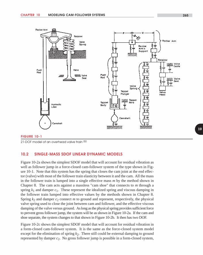
Nevertheless, others have developed multi-DOF lumped-parameter models for thisapplication. Seidlitz[6] describes a 21-DOF model of a pushrod overhead valve train asshown in Figure 10-1 in which he used one DOF for the camshaft, two for the hydraulictappet, two for the pushrod, four for the rocker arm, one for the spring retainer, two forthe valve, and nine for the valve spring. Two of the dampers were nonlinear. From thisextensive numerical simulation that correlated well with experimental measurements heconcludes that:
In spite of the presence of some nonlinear damping and three-dimensional motions, avalve train can be viewed as a linear, one-dimensional mechanical system with tworesonant frequencies. The first mode is predominately the first axial mode of thevalve spring with the highest modal motion at the middle of the valve spring. Thesecond mode is predominately the remainder of the valve train stretching andcompressing along its axial length with the highest modal motion at the valvehead.[7]
This recommends a two-DOF model that can separate the spring and follower train.
Pisano[8] used a combined lumped and distributed parameter model of a valve train andconfirmed its accuracy experimentally. Regarding the model, he concludes:
The incorporation of a distributed parameter element (helical valve spring) is crucialto the formulation of an accurate predictive model of a high-speed cam-followersystem . . . The careful modeling of the valve spring as a distributed parameter(continuum) component is the key to success of the complete dynamic model . . .[9]
* Universal TechnicalServices, 1220 Rock St.,Rockford, IL 61101.www.uts.com
† Mathsoft Inc., 101 MainSt. Cambridge, MA 02142.www.mathsoft.com
‡ The MathWorks Inc., 24Prime Park Way, Natick,Massachusetts, 01760.www.mathworks.com
CHAPTER 10 MODELING CAM-FOLLOWER SYSTEMS 265
10
FIGURE 10-1
21-DOF model of an overhead valve train [6]
10.2 SINGLE-MASS SDOF LINEAR DYNAMIC MODELS
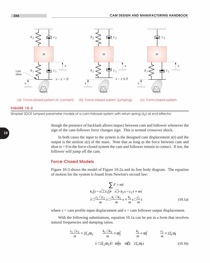
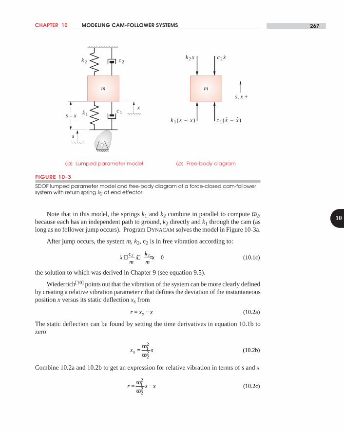
Figure 10-2a shows the simplest SDOF model that will account for residual vibration aswell as follower jump in a force-closed cam-follower system of the type shown in Fig-ure 10-1. Note that this system has the spring that closes the cam joint at the end effec-tor (valve) with most of the follower train elasticity between it and the cam. All the massin the follower train is lumped into a single effective mass m by the method shown inChapter 8. The cam acts against a massless "cam shoe" that connects to m through aspring k1 and damper c1. These represent the idealized spring and viscous damping inthe follower train lumped into effective values by the methods shown in Chapter 8.Spring k2 and damper c2 connect m to ground and represent, respectively, the physicalvalve spring used to close the joint between cam and follower, and the effective viscousdamping of the valve versus ground. As long as the physical spring provides sufficient forceto prevent gross follower jump, the system will be as shown in Figure 10-2a. If the cam andshoe separate, the system changes to that shown in Figure 10-2b. It then has two DOF.
Figure 10-2c shows the simplest SDOF model that will account for residual vibration ina form-closed cam-follower system. It is the same as the force-closed system modelexcept for the elimination of spring k2. There still could be external damping to groundrepresented by damper c2. No gross follower jump is possible in a form-closed system,
CAM DESIGN AND MANUFACTURING HANDBOOK266
10
though the presence of backlash allows impact between cam and follower whenever thesign of the cam-follower force changes sign. This is termed crossover shock.
In both cases the input to the system is the designed cam displacement s(t) and theoutput is the motion x(t) of the mass. Note that as long as the force between cam andshoe is > 0 in the force-closed system the cam and follower remain in contact. If not, thefollower will jump off the cam.
Force-Closed Models
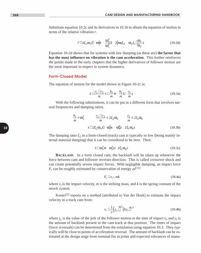
Figure 10-3 shows the model of Figure 10-2a and its free body diagram. The equationof motion for the system is found from Newton's second law:
F mx
k s x c s x k x c x mx
xc c
mx
k k
mx
k
ms
c
ms
=
−( ) + −( ) − − =
+ + + + = +
∑ ˙
˙ ˙ ˙ ˙
˙ ˙ ˙
1 1 2 2
1 2 1 2 1 1 (10.1a)
where s = cam profile input displacement and x = cam follower output displacement.
With the following substitutions, equation 10.1a can be put in a form that involvesnatural frequencies and damping ratios.
c c
m
k k
m
k
m
c
m
x x x s s
1 22 2
1 222 1
12 1
1 1
2 2 22
12
1 1
2 2
2 2
+ = + = = =
+ + = +
ζ ω ω ω ζ ω
ζ ω ω ω ζ ω˙ ˙ ˙ (10.1b)
FIGURE 10-2
Simplest SDOF lumped parameter models of a cam-follower system with return spring (k2) at end effector
(a) Force-closed system (in contact)
k1 c1
k2 c2
x
s
m
(b) Force-closed system (jumping)
k1 c1
k2 c2
x
s
m
(c) Form-closed system
c1
c2
x
s
m
k1
s – x > 0 s – x ≤ 0
camshoe
CHAPTER 10 MODELING CAM-FOLLOWER SYSTEMS 267
10Note that in this model, the springs k1 and k2 combine in parallel to compute ω2,
because each has an independent path to ground, k2 directly and k1 through the cam (aslong as no follower jump occurs). Program DYNACAM solves the model in Figure 10-3a.
After jump occurs, the system m, k2, c2 is in free vibration according to:
˙ ˙xc
mx
k
mx+ + =2 2 0 (10.1c)
the solution to which was derived in Chapter 9 (see equation 9.5).
Wiederrich[10] points out that the vibration of the system can be more clearly definedby creating a relative vibration parameter r that defines the deviation of the instantaneousposition x versus its static deflection xs from
r x xs= − (10.2a)
The static deflection can be found by setting the time derivatives in equation 10.1b tozero
x ss = ωω
12
22 (10.2b)
Combine 10.2a and 10.2b to get an expression for relative vibration in terms of s and x
r s x= −ωω
12
22 (10.2c)
FIGURE 10-3
SDOF lumped parameter model and free-body diagram of a force-closed cam-follower system with return spring k2 at end effector
(b) Free-body diagram
m
k1(s – x)
k2x c2x.
c1(s – x). .
(a) Lumped parameter model
k1c1
k2 c2
x
s
m
s – x
s, x +
CAM DESIGN AND MANUFACTURING HANDBOOK268
10
Substitute equation 10.2c and its derivatives in 10.1b to obtain the equation of motion interms of the relative vibration r.
˙ ˙ ˙ ˙r r r s s+ + = + −( )2 22 2 22 1
2
22 1 2 2 1
1
2ζ ω ω ω
ωω ζ ω ζ ω
ω(10.2d)
Equation 10-2d shows that for systems with low damping (as these are) the factor thathas the most influence on vibration is the cam acceleration. This further reinforcesthe points made in the early chapters that the higher derivatives of follower motion arethe most important in respect to system dynamics.
Form-Closed Model
The equation of motion for the model shown in Figure 10-2c is:
˙ ˙ ˙xc c
mx
k
mx
k
ms
c
ms+ + + = +1 2 1 1 1 (10.3a)
With the following substitutions, it can be put in a different form that involves nat-ural frequencies and damping ratios.
k
m
c c
m
c
m
x x x s s
n n n
n n n n
1 2 1 22
11
22 2
1
2 2
2 2
= + = =
+ + = +
ω ζ ω ζ ω
ζ ω ω ω ζ ω˙ ˙ ˙ (10.3b)
The damping ratio ζ2 in a form-closed (track) cam is typically so low (being mainly in-ternal material damping) that it can be considered to be zero. Then:
˙ ˙x x s sn n n+ = +ω ω ζ ω2 212 (10.3c)
BACKLASH In a form closed cam, the backlash will be taken up whenever theforce between cam and follower reverses direction. This is called crossover shock andcan create potentially severe impact forces. With negligible damping, an impact forceFi can be roughly estimated by conservation of energy as[11]
F v mki i≅ (10.4a)
where vi is the impact velocity, m is the striking mass, and k is the spring constant of thestruck system.
Koster[2] reports on a method (attributed to Van der Hoek) to estimate the impactvelocity in a track cam from:
v j yi t ii≅ ( ) ( )1
26
1 3 2 3(10.4b)
where jti is the value of the jerk of the follower motion at the time of impact ti, and yi isthe amount of backlash present in the cam track at that position. The times of impact(force reversals) can be determined from the simulation using equation 10.3. They typ-ically will be close to points of acceleration reversal. The amount of backlash can be es-timated at the design stage from nominal fits in joints and expected tolerances of manu-
CHAPTER 10 MODELING CAM-FOLLOWER SYSTEMS 269
10
facture of cam and roller follower. For an existing system, backlash is easily measuredwith a dial indicator. It can be seen from equations 10.4 that for any amount of irreduciblebacklash, the impact force can be reduced by choosing a cam function with lower values ofjerk at the points of acceleration reversal. Also, wear will increase backlash over time.
10.3 TWO-MASS, ONE- OR TWO-DOF, NONLINEAR DYNAMIC MODELOF A VALVE TRAIN
The simple models described in the previous section are considered to be adequate formany cam-follower systems such as valve trains where the spring is at the end effector,particularly if the mass at the end effector is relatively large compared to the mass of thefollower train components closer to the cam, if jump is unlikely, damping is not domi-nated by coulomb friction, and if the follower is never deliberately held off the cam (suchas during a dwell). If these conditions are not true, then a more elaborate model is need-ed to give a better prediction of follower dynamics.
Barkan[1] developed a model for the automotive valve train that, with slight refine-ments by others,[3],[4] has proven to quite accurately predict the behavior of this moredynamically complicated cam-follower system.
Barkan showed that including a coulomb damper as well as a viscous damper sig-nificantly improved the model. The viscous damping ratio was assumed to be between0.02 and 0.15, based on the literature. A coulomb friction coefficient of 0.2 was used.Barkan also includes the gas force acting on the valve head.
Akiba added a second lumped mass at the cam.[3] This better predicts cam contactforce, and thus jump, than the single mass model.[4] The two-mass model also becomesa 2-DOF system after jump occurs, giving a more realistic and accurate simulation. Themodel also provides for contact between valve and valve seat at closure.
For proper engine operation, a valve train must ensure tight closure of the valveduring dwell, both to eliminate blowby and to give the valves (especially the exhaustvalve) good coupling for heat transfer to the valve seat. This is accomplished by eithermaintaining a deliberate clearance (valve lash) between the cam follower and cam dur-ing the dwell, or providing a hydraulic lash adjuster as a compliant link between the two. Thisalso compensates for the thermal expansion of the follower train at operating temperature.
An analogous condition is often encountered in industrial machinery when a follow-er train is brought back to a "hard stop" on the ground plane just short of the low dwell.A hard stop is sometimes needed when the cam is interrupted and leaves the follower forpart of the low dwell or it may be needed to guarantee follower train position during thelow dwell to a greater mechanical accuracy than can be obtained from the cam, giventhe stack-up of assembly tolerances and dynamic deflections.
In both of these situations, there is an impact event when the follower train hits thehard stop (or valve seat) with some velocity, and again at the beginning of the rise as thecam encounters the stationary follower with some velocity. The cam design in thesecases often contains constant velocity "ramps" at the beginning and end of the rise to con-trol the magnitude of the impact velocities over a range of tolerance of the impact point.
CAM DESIGN AND MANUFACTURING HANDBOOK270
10
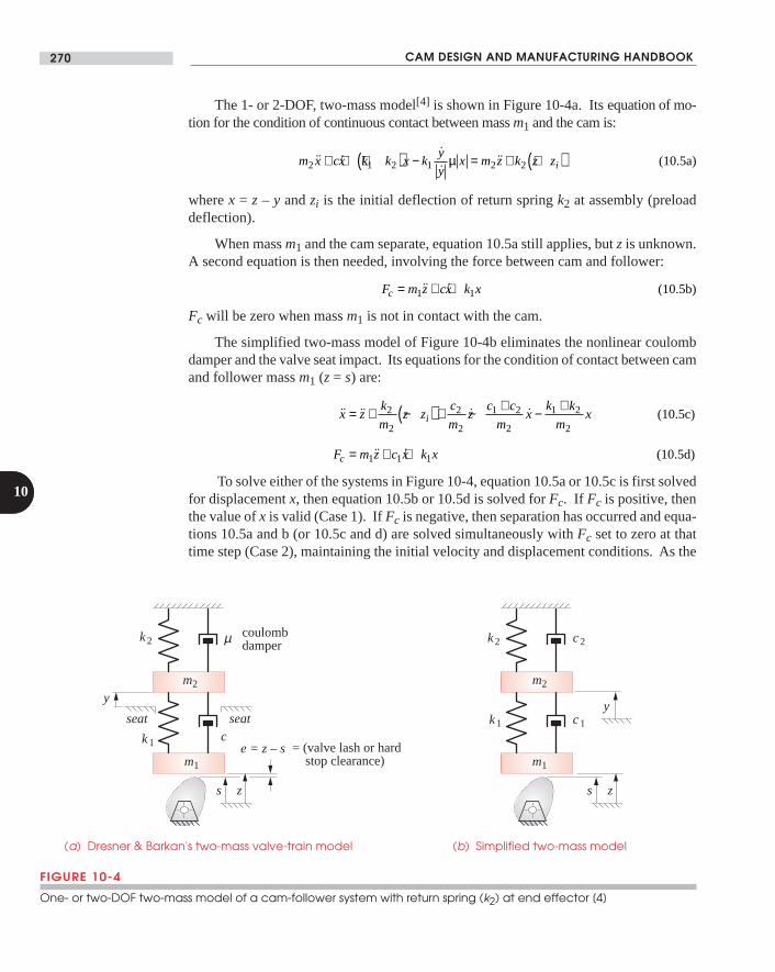
The 1- or 2-DOF, two-mass model[4] is shown in Figure 10-4a. Its equation of mo-tion for the condition of continuous contact between mass m1 and the cam is:
m x cx k k x ky
yx m z k z zi2 1 2 1 2 2˙ ˙
˙
˙˙+ + +( ) − = + +( )µ (10.5a)
where x = z – y and zi is the initial deflection of return spring k2 at assembly (preloaddeflection).
When mass m1 and the cam separate, equation 10.5a still applies, but z is unknown.A second equation is then needed, involving the force between cam and follower:
F m z cx k xc = + +1 1˙ ˙ (10.5b)
Fc will be zero when mass m1 is not in contact with the cam.
The simplified two-mass model of Figure 10-4b eliminates the nonlinear coulombdamper and the valve seat impact. Its equations for the condition of contact between camand follower mass m1 (z = s) are:
˙ ˙ ˙ ˙x zk
mz z
c
mz
c c
mx
k k
mxi= + −( ) + − + − +2
2
2
2
1 2
2
1 2
2(10.5c)
F m z c x k xc = + +1 1 1˙ ˙ (10.5d)
To solve either of the systems in Figure 10-4, equation 10.5a or 10.5c is first solvedfor displacement x, then equation 10.5b or 10.5d is solved for Fc. If Fc is positive, thenthe value of x is valid (Case 1). If Fc is negative, then separation has occurred and equa-tions 10.5a and b (or 10.5c and d) are solved simultaneously with Fc set to zero at thattime step (Case 2), maintaining the initial velocity and displacement conditions. As the
FIGURE 10-4
One- or two-DOF two-mass model of a cam-follower system with return spring (k2) at end effector [4]
(b) Simplified two-mass model(a) Dresner & Barkan's two-mass valve-train model
k1 c
k2 µ
s z
seat seat
y
coulomb damper
m1
e = z – s= (valve lash or hard stop clearance)
k1
k2
s z
m1
yc1
c2
m2 m2
CHAPTER 10 MODELING CAM-FOLLOWER SYSTEMS 271
10
solution continues for additional time steps, s and z are compared at each step. When zbecomes ≤ s, the cam and follower have regained contact and the solution reverts to Case1, maintaining the initial condition for dx/dt but changing the initial condition for dz/dtto match the cam velocity. This assumes a coefficient of restitution of zero on impact,which does not accurately model the impact event but is valid after the follower stopsbouncing on the cam. When a transition is made from one case to the other, the time atwhich Fc changes sign must be found by iteration in order to maximize accuracy.[4]
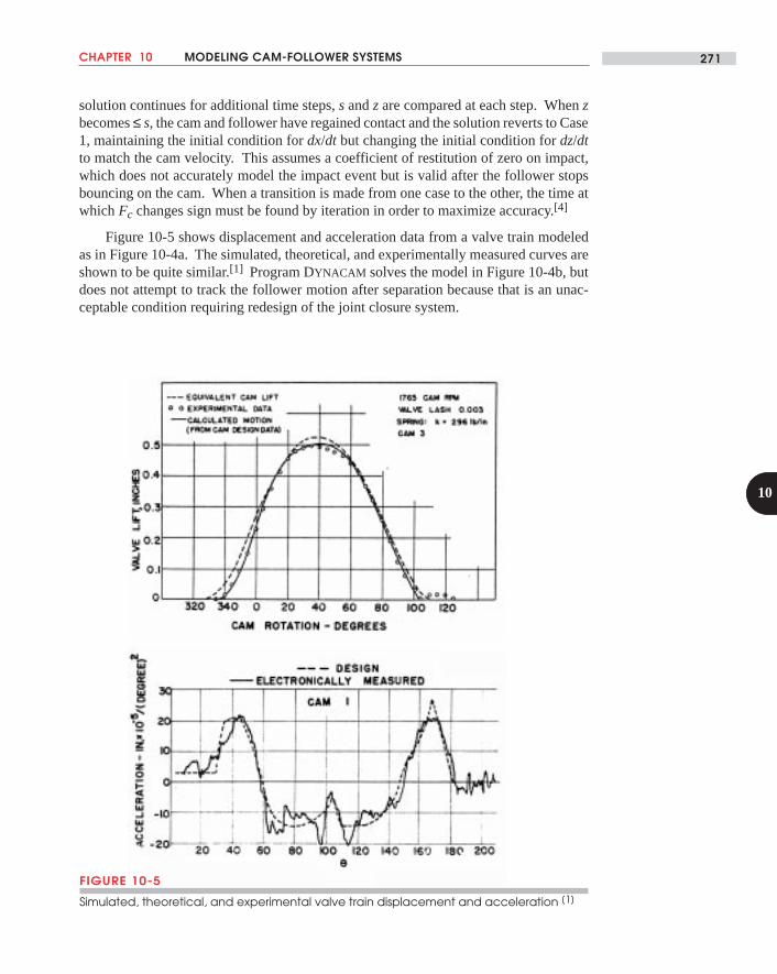
Figure 10-5 shows displacement and acceleration data from a valve train modeledas in Figure 10-4a. The simulated, theoretical, and experimentally measured curves areshown to be quite similar.[1] Program DYNACAM solves the model in Figure 10-4b, butdoes not attempt to track the follower motion after separation because that is an unac-ceptable condition requiring redesign of the joint closure system.
FIGURE 10-5
Simulated, theoretical, and experimental valve train displacement and acceleration [1]
CAM DESIGN AND MANUFACTURING HANDBOOK272
10
10.4 MULTI-DOF DYNAMIC MODEL OF A VALVE TRAIN
Seidlitz[6] built the 21-DOF model of a valve train shown in Figure 10-1 (p. 265). A briefdescription of his modeling techniques and assumptions will be given here as a guide tothe reader wishing to create a multi-DOF model of a different cam-follower system.More detail can be found in the original reference, which is quite complete.
Springs and/or dampers attach the model to ground at the camshaft, hydraulic tap-pet, rocker arm center, valve center, valve head, and the bottom of the valve spring. Thecamshaft was modeled as one mass, spring, and damper system, with its mass being thatof one cam lobe plus half of the remaining mass between the cam bearings. Its springrate was that of the camshaft in bending at the cam lobe.
The hydraulic tappet model had two masses, one spring, and two dampers. Thespring rate of the tappet's oil column was "backed out" of the model (when run) by ad-justing its value to get good correlation with experimental data. This method is common-ly used in dynamic modeling to estimate values of elements (particularly dampers) thatare difficult to either calculate or measure directly. A dead band was also built into the modelcalculation to simulate the lost motion associated with the tappets's internal check valve.
The pushrod was modeled as two masses, each half its total mass, three springs, andthree dampers. The end springs each had the same stiffness but were twice the stiffnessof the center spring. The combined spring rate of the three springs in series equaled thatof the actual pushrod.
The rocker arm was modeled as three masses, one inertia, three springs, and fourdampers. One mass was placed at each end of the arm and one at its center. The rota-tional inertia value applied at the center mass was the actual arm's inertia minus the ef-fective inertia of the two end masses. Each end spring represented the effective springrate from the center of the arm to that end. These values were determined by a staticforce-deflection measurement on the rocker arm. (Nowadays, if a solids model of a pro-posed design exists, it is a short step to make FEA models of its elements such as rockerarms and determine their spring rates before any metal is cut.)
The valve spring was modeled as nine masses, ten springs, and ten dampers. Thetotal spring mass was divided by the number of coils, and one coil's worth assigned toeach of the end masses. The remaining mass was divided equally among the remainingseven lumped masses. The two end springs were made ten times stiffer than the middlesprings. This made the middle springs 8.2 times as stiff as that of the actual valve spring.Each value could be entered separately in the model allowing any combination of mass-es, springs, and dampers to mimic alternate spring designs. Coil-to-coil contact was sim-ulated and when coils touched in the simulation, their spring and damper values wereincreased by a hundredfold. By varying clearances between coils in the model, a vari-able rate spring could be simulated. (A variable-rate valve spring typically is wound witha varying coil pitch. As the spring compresses, the close-spaced coils contact one anoth-er and thus increase the spring rate dynamically.)
Camshaft speed was assumed constant. The cam lift profile was entered into themodel as an array of lift values at half-degree intervals and smoothed with a 5th-order
CHAPTER 10 MODELING CAM-FOLLOWER SYSTEMS 273
10
polynomial for sampling at the model's calculation times. The system equation waswritten in matrix form:
M C K[ ] + [ ] + [ ] = ( )˙ ˙x x x F t (10.6)
where M is the mass matrix, C is the damping matrix, and K is the stiffness matrix forthe system. This matrix equation was solved with a custom-written computer program.Damping coefficients that are difficult to determine independently were adjusted to ob-tain good correlation of the simulation with experimental measurements made of the ac-tual valve train. Once a model such as this is "tuned" to match experimental data, it be-comes a tool that can be used to investigate the dynamic effects of proposed designchanges, or entirely new but similar designs, in advance of their implementation in hard-ware.
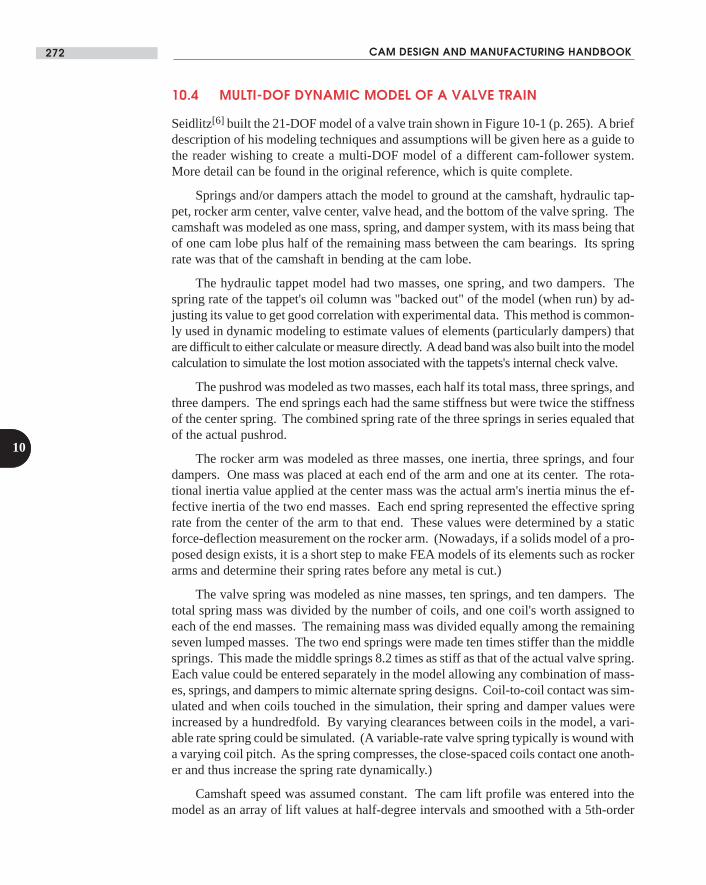
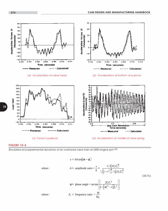
Figure 10-6 shows a sample of the simulated and experimental data, superposed.Good correlation between the simulation and experiment can be seen in the accelerationplots of valve head and pushrod. The pushrod force shows reasonable correlation, asdoes the acceleration at the middle of the spring. While a great deal of effort is requiredto create and verify a model of this complexity, when done, it can give a wealth of dy-namic information about that system and about similar systems yet to be built.
10.5 ONE-MASS MODEL OF AN INDUSTRIAL CAM-FOLLOWER SYSTEM
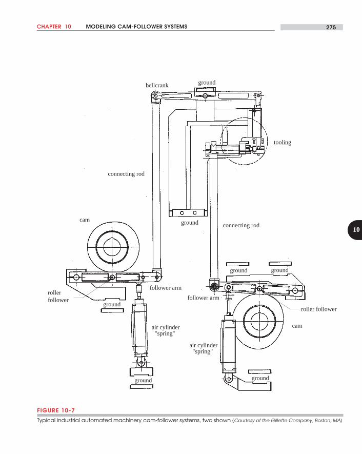
The models described in the previous sections are all directed at the automotive valvetrain application, particularly the overhead-valve pushrod type. They have been shownto agree quite closely with experimental data from those mechanisms. However, thesemodels may not provide a good representation of the typical industrial cam-follower trainas used in automated machinery. These systems often look like Figure 10-7 where the fol-lower spring (or air-cylinder "spring") connects the follower to ground close to the cam rath-er than at the end effector, as it is in the case of the overhead valve train of Figure 10-1.*
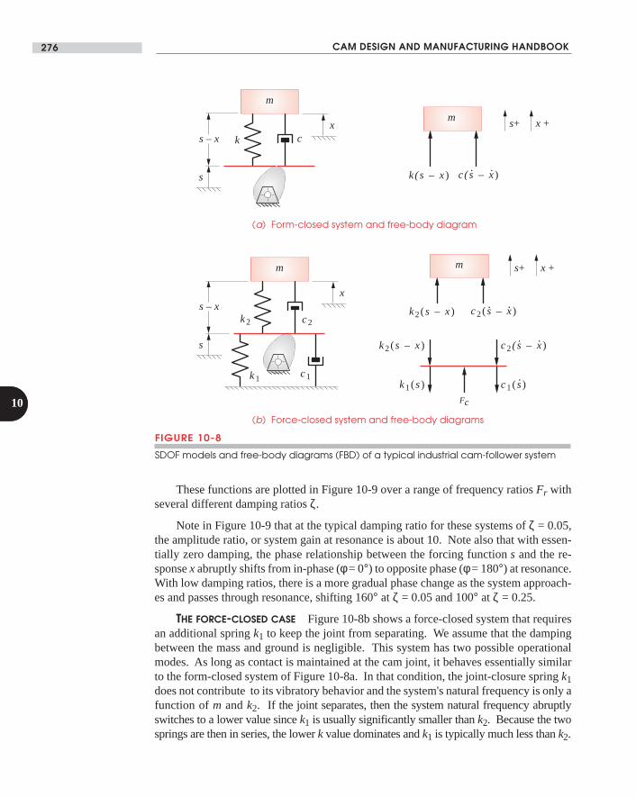
Figure 10-8 shows SDOF models and free-body diagrams of this system for the form-closed and force-closed cam cases, their difference being the additional spring needed tomaintain contact of the cam joint in the latter case, along with its associated damping.
THE FORM-CLOSED CASE Figure 10-8a shows an example of the classic, base-ex-cited SDOF system found in any introductory text on vibration theory if we assume thatthe damping between the mass and ground is negligible. Its system equation is foundfrom summing forces on the free-body diagram (FBD) of Figure 10-8a.
˙ ˙ ˙xc
mx
k
mx
k
ms
c
ms+ + = + (10.7a)
where :
then : (10.7b)
k
m
c
m
x x x s s
n n
n n n n
= =
+ + = +
ω ζω
ζω ω ω ζω
2
2 2
2
2 2
,
˙ ˙ ˙
Its response to an harmonic excitation of the base, s(t) = h sin(ωt), is given by:
* Note that some industrialcam-follower trains havethe joint closure springplaced at the end effectorin order to load all the jointclearances in one directionand take out the backlashin the system. If this isdone, then the valve trainmodel gives a betterrepresentation of itsdynamic behavior.Program DYNACAM
provides both dynamicmodels for analysis.
CAM DESIGN AND MANUFACTURING HANDBOOK274
10
FIGURE 10-6
Simulated and experimental dynamics of an overhead valve train at 2400 engine rpm [6]
(b) Acceleration at bottom of pushrod
(d) Acceleration at middle of valve spring (c) Force in pushrod
(a) Acceleration of valve head
x Ah t
Ax
h
F
r F
F
F
F
r
r
r
r
rn
= −( )
= =+ ( )
−( ) + ( )
=−( )
=
sin
arctan
ω φ
ζ
ζ
φ ζζ
ωω
where : amplitude ratio =
(10.7c)
phase angle =1+ 4
where : frequency ratio =
2
1 2
1 2
2
1
2
2 2 2
3
2
CHAPTER 10 MODELING CAM-FOLLOWER SYSTEMS 275
10
cam
camair cylinder "spring"
ground ground
ground
ground
ground
connecting rod
connecting rod
bellcrank
follower arm
follower arm
tooling
ground ground
rollerfollower
roller follower
air cylinder "spring"
FIGURE 10-7
Typical industrial automated machinery cam-follower systems, two shown (Courtesy of the Gillette Company, Boston, MA)
CAM DESIGN AND MANUFACTURING HANDBOOK276
10
These functions are plotted in Figure 10-9 over a range of frequency ratios Fr withseveral different damping ratios ζ.
Note in Figure 10-9 that at the typical damping ratio for these systems of ζ = 0.05,the amplitude ratio, or system gain at resonance is about 10. Note also that with essen-tially zero damping, the phase relationship between the forcing function s and the re-sponse x abruptly shifts from in-phase (φ = 0°) to opposite phase (φ = 180°) at resonance.With low damping ratios, there is a more gradual phase change as the system approach-es and passes through resonance, shifting 160° at ζ = 0.05 and 100° at ζ = 0.25.
THE FORCE-CLOSED CASE Figure 10-8b shows a force-closed system that requiresan additional spring k1 to keep the joint from separating. We assume that the dampingbetween the mass and ground is negligible. This system has two possible operationalmodes. As long as contact is maintained at the cam joint, it behaves essentially similarto the form-closed system of Figure 10-8a. In that condition, the joint-closure spring k1does not contribute to its vibratory behavior and the system's natural frequency is only afunction of m and k2. If the joint separates, then the system natural frequency abruptlyswitches to a lower value since k1 is usually significantly smaller than k2. Because the twosprings are then in series, the lower k value dominates and k1 is typically much less than k2.
FIGURE 10-8
SDOF models and free-body diagrams (FBD) of a typical industrial cam-follower system
(b) Force-closed system and free-body diagrams
(a) Form-closed system and free-body diagram
x
s
s – x
m
k c
k1 c1
x
s
s – x
m
k2 c2
m
k2(s – x)
s+ x +
m
k(s – x) c(s – x). .
s+ x +
k1(s)
k2(s – x)
c1(s).
c2(s – x). .
c2(s – x). .
Fc

CHAPTER 10 MODELING CAM-FOLLOWER SYSTEMS 277
10
If we assume that contact between cam and follower is somehow maintained at alltimes, then the system equation is the same as that of equation 10.7, repeated here usingnotation consistent with Figure 10-8b.
˙ ˙ ˙xc
mx
k
mx
k
ms
c
ms+ + = +2 2 2 2 (10.8a)
where :
then : (10.8b)
k
m
c
m
x x x s s
222 2
2 2
2 2 22
22
2 2
2
2 2
= =
+ + = +
ω ζ ω
ζ ω ω ω ζ ω
,
˙ ˙ ˙
If the joint separates, then the system equation becomes:
˙ ˙ ˙xc
mx
k
mx
k
ms
c
ms
eff eff eff eff+ + = + (10.9a)
0 0.5 1.0 1.5 2.0 2.5 3.0
0
1
2
3
4
5
6
7
8
10
9
Frequency Ratio Fr = ω / ωn
Am
plitu
de R
atio
x /
h
0.05
0.10
0.15
ζ = 0.001
0.25
0 0.5 1.0 1.5 2.0 2.5 3.0
0
20
40
60
80
100
120
140
160
180
Pha
se A
ngle
(de
g)
0.050.100.15
ζ = 0.001
0.25
Frequency Ratio Fr = ω / ωnFIGURE 10-9
Amplitude ratio and phase angle of a harmonically base-excited SDOF system
CAM DESIGN AND MANUFACTURING HANDBOOK278
10
where :
then : (10.9b)
* kk k
k kc
c c
c c
k
m
c
m
x x x s s
eff effeff eff=
+=
+= =
+ + = +
1 2
1 2
1 2
1 212
1 1
1 1 12
12
1 1
2
2 2
ω ζ ω
ζ ω ω ω ζ ω˙ ˙ ˙
Program DYNACAM solves both of the models in Figure 10-8 (p. 276).
This system, though of only one DOF, has two natural frequencies, one when in con-tact, and another when separated. The question then becomes: under what conditionswill it separate? Looking at Figure 10-9 (p. 277), which depicts the in-contact case, itwould appear that, with the damping typical in these systems (ζ = 0.05 to 0.10), one couldoperate at frequency ratios lower than about ω2 / 3 and expect no separation, providedthat the closure spring rate k1 and preload had been properly selected by the kinetostatictechnique shown in Chapter 9 in order to avoid gross kinematic jump.
But what will happen if the operating speed ω chosen on that basis happens to beclose to, or above, the lower, separation natural frequency ω1 of the system? This is en-tirely possible if the follower train is stiff compared to the closure spring (k2 >> k1). Thissituation is both common and desirable in cam-follower systems. We want the stiffestpossible follower train in order to minimize the dynamic error (s – x). If k2 were infinite,then x would equal s, giving zero error. We also do not want the closure spring stiffnessk1 to be any greater than is needed to prevent kinematic jump, because its force, in part,determines the stresses in the cam and follower.
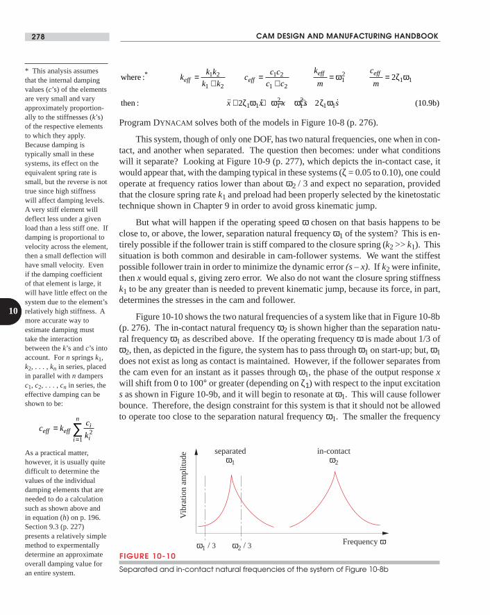
Figure 10-10 shows the two natural frequencies of a system like that in Figure 10-8b(p. 276). The in-contact natural frequency ω2 is shown higher than the separation natu-ral frequency ω1 as described above. If the operating frequency ω is made about 1/3 ofω2, then, as depicted in the figure, the system has to pass through ω1 on start-up; but, ω1does not exist as long as contact is maintained. However, if the follower separates fromthe cam even for an instant as it passes through ω1, the phase of the output response xwill shift from 0 to 100° or greater (depending on ζ1) with respect to the input excitations as shown in Figure 10-9b, and it will begin to resonate at ω1. This will cause followerbounce. Therefore, the design constraint for this system is that it should not be allowedto operate too close to the separation natural frequency ω1. The smaller the frequency
FIGURE 10-10
Separated and in-contact natural frequencies of the system of Figure 10-8b
Vib
ratio
n am
plitu
de
Frequency ωω2 / 3ω1 / 3
ω1
separatedω2
in-contact
* This analysis assumesthat the internal dampingvalues (c’s) of the elementsare very small and varyapproximately proportion-ally to the stiffnesses (k’s)of the respective elementsto which they apply.Because damping istypically small in thesesystems, its effect on theequivalent spring rate issmall, but the reverse is nottrue since high stiffnesswill affect damping levels.A very stiff element willdeflect less under a givenload than a less stiff one. Ifdamping is proportional tovelocity across the element,then a small deflection willhave small velocity. Evenif the damping coefficientof that element is large, itwill have little effect on thesystem due to the element’srelatively high stiffness. Amore accurate way toestimate damping musttake the interactionbetween the k’s and c’s intoaccount. For n springs k1,k2, . . . , kn in series, placedin parallel with n dampersc1, c2, . . . , cn in series, theeffective damping can beshown to be:
c kc
keff eff
i
ii
n
==∑ 2
1
As a practical matter,however, it is usually quitedifficult to determine thevalues of the individualdamping elements that areneeded to do a calculationsuch as shown above andin equation (h) on p. 196.Section 9.3 (p. 227)presents a relatively simplemethod to expermentallydetermine an approximateoverall damping value foran entire system.
CHAPTER 10 MODELING CAM-FOLLOWER SYSTEMS 279
10
ratio ω / ω1 the better. Usually a ratio of about ω1 / 3 or less will be sufficient to avoidseparation and follower jump. The follower spring stiffness k1, rather than the followertrain stiffness k2, then limits the system operating speed ω.
10.6 TWO-MASS MODEL OF AN INDUSTRIAL CAM-FOLLOWER SYSTEM
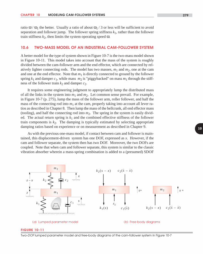
A better model for the type of system shown in Figure 10-7 is the two-mass model shownin Figure 10-11. This model takes into account that the mass of the system is roughlydivided between the cam-follower arm and the end effector, which are connected by rel-atively lighter connecting rods. The model has two masses, m1 and m2, one at the camand one at the end effector. Note that m1 is directly connected to ground by the followerspring k1 and damper c1, while mass m2 is "piggybacked" on mass m1 through the stiff-ness of the follower train k2 and damper c2.
It requires some engineering judgment to appropriately lump the distributed massof all the links in the system into m1 and m2. Let common sense prevail. For example,in Figure 10-7 (p. 275), lump the mass of the follower arm, roller follower, and half themass of the connecting rod into m1 at the cam, properly taking into account all lever ra-tios as described in Chapter 8. Then lump the mass of the bellcrank, all end effector mass(tooling), and half the connecting rod into m2. The spring in the system is easily divid-ed. The actual return spring is k1 and the combined effective stiffness of the followertrain components is k2. The damping is typically estimated by selecting appropriatedamping ratios based on experience or on measurement as described in Chapter 9.
As with the previous one-mass model, if contact between cam and follower is main-tained, this displacement-driven system has one DOF, expressed as x. However, if thecam and follower separate, the system then has two DOF. Moreover, the two DOFs arecoupled. Note that when cam and follower separate, this system is similar to the classicvibration absorber wherein a mass-spring combination is added to a (presumed) SDOF
FIGURE 10-11
Two-DOF lumped parameter model and free-body diagrams of the cam-follower system in Figure 10-7
(b) Free-body diagrams(a) Lumped parameter model
k1c1
k2 c2
x
z
z – x
m2
m1m1
k1(s)
k2(s – x) c2(s – x). .
c1(s).
m2
k2(s – x) c2(s – x). .
s+ x +
sFc
CAM DESIGN AND MANUFACTURING HANDBOOK280
10
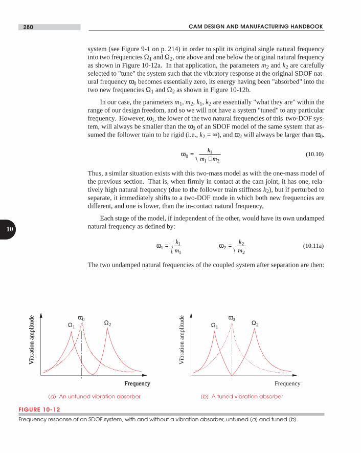
FIGURE 10-12
Frequency response of an SDOF system, with and without a vibration absorber, untuned (a) and tuned (b)
(a) An untuned vibration absorber (b) A tuned vibration absorber
Vib
ratio
n am
plitu
de
Frequency
Vib
ratio
n am
plitu
de
Frequency
Vib
ratio
n am
plitu
de
Frequency
ω0 Ω2Ω1
ω0 Ω2Ω1
system (see Figure 9-1 on p. 214) in order to split its original single natural frequencyinto two frequencies Ω1 and Ω2, one above and one below the original natural frequencyas shown in Figure 10-12a. In that application, the parameters m2 and k2 are carefullyselected to "tune" the system such that the vibratory response at the original SDOF nat-ural frequency ω0 becomes essentially zero, its energy having been "absorbed" into thetwo new frequencies Ω1 and Ω2 as shown in Figure 10-12b.
In our case, the parameters m1, m2, k1, k2 are essentially "what they are" within therange of our design freedom, and so we will not have a system "tuned" to any particularfrequency. However, ω1, the lower of the two natural frequencies of this two-DOF sys-tem, will always be smaller than the ω0 of an SDOF model of the same system that as-sumed the follower train to be rigid (i.e., k2 = ∞), and ω2 will always be larger than ω0.
ω01
1 2=
+k
m m(10.10)
Thus, a similar situation exists with this two-mass model as with the one-mass model ofthe previous section. That is, when firmly in contact at the cam joint, it has one, rela-tively high natural frequency (due to the follower train stiffness k2), but if perturbed toseparate, it immediately shifts to a two-DOF mode in which both new frequencies aredifferent, and one is lower, than the in-contact natural frequency,
Each stage of the model, if independent of the other, would have its own undampednatural frequency as defined by:
ω ω11
12
2
2= =k
m
k
m(10.11a)
The two undamped natural frequencies of the coupled system after separation are then:
CHAPTER 10 MODELING CAM-FOLLOWER SYSTEMS 281
10
Ω1 21 2 4 2 2
2 2
1
21 1 1 2 1 1, = + +( ) ± +( ) + −( ) +
=
ω
ωω
q u q u u q
q um
m
(10.11b)
where : =1
Note that both Ω1 and Ω2 are functions of the mass ratio m2 / m1 and the frequency ratioω2 / ω1, which includes the spring rates k1 and k2.*
Summing forces and applying Newton's 2nd law to the free-body diagrams of Fig-ure 10-11 gives, for the in-contact case:
m x c z x k z x
xc
mz
k
mz
c
mx
k
mx
x z z x x
2 2 2
2
2
2
2
2
2
2
2
2 2 22
2 2 222 2
˙ ˙ ˙
˙ ˙ ˙
˙ ˙ ˙
= −( ) + −( )
= + − −
= + − −ζ ω ω ζ ω ω (10.12a)
where, if contact is maintained, z = s. The contact force Fc is found from:
m z F c z k z c z x k z x
F m z c c z k k z c x k x
c
c
1 1 1 2 2
1 2 1 2 1 2 2
˙ ˙ ˙ ˙
˙ ˙ ˙
= − − − −( ) − −( )= + +( ) + +( ) − − (10.12b)
When separation occurs, the contact force Fc becomes zero.
To solve this system, first assume that cam and follower are in contact, (z = s), andsolve equation 10.12a for x. Use the value for x at that time step to find Fc from equa-tion 10.12b. If Fc > 0, then the cam and follower are in contact at that time and the com-puted value of x is valid. If Fc < 0, then separation has occurred, z > s and the computedvalue of x is invalid. Then set Fc to zero and solve equations 10.12a and b simultaneous-ly for x and z. Continue this second solution approach, testing z against s at each timestep. When z ≤ s, contact has reoccurred, and equation 10.12a can again be used aloneto solve for x until a negative value of Fc is again encountered. Thus the solution mustswitch between the two solution cases based on the sign of Fc. Note also that when thesolution is switched from one stage to the other, the most recent values of x, z and theirderivatives must be used as initial conditions for the next stage of the solution.
From a practical standpoint, since separation of cam and follower is generally unac-ceptable in these systems, the solution process could be aborted when the force goesnegative and the designer then prompted to modify the system parameters to correct theproblem. For example, increasing the stiffness and/or reducing the mass of the followersystem may cure the problem as will increasing the stiffness or preload of the closurespring. Redesigning the cam function to reduce the negative peak acceleration will alsoimprove the situation. Program DYNACAM solves the two-mass model of Figure 10-11as described in this paragraph.
* As an aside, thedeliberate addition of tunedvibration absorbers to acam-follower system suchas is shown in Figure 10-7can be a very effective wayto reduce vibration at anyoperating speeds that areclose to the system'snatural frequencies. Infact, one could introducetwo such mass-springabsorbers to the system ofFigure 10-7, as modeled inFigure 10-11, one mountedon mass m1 and anothermounted on mass m2 totune their respectiveresponses to zero at theoperating speed.
CAM DESIGN AND MANUFACTURING HANDBOOK282
10
10.7 SOLVING SYSTEM DIFFERENTIAL EQUATIONS
The closed-form solution to the classic linear, second-order, constant-coefficient ordi-nary differential equation (ODE) was presented in Chapter 9. That solution is only validfor that particular type of ODE. Though equations 10.1 are in that category, other modelsof cam follower systems involve nonconstant and nonlinear coefficients and so cannotbe solved by traditional closed-form analytical methods. For such equations, which oc-cur frequently in the modeling of dynamic systems, a numerical method of solution isneeded. Many such algorithms exist. The Runge-Kutta methods are perhaps the bestknown, but there also are other methods that may be superior in some instances.[21]
Block Diagram Solution—Simulink/MatLab
Many computer packages are now available that will solve even complicated differen-tial equations numerically (and symbolically in some cases). One such is MATLAB whichcontains a simulation package called SIMULINK . This "front-end" to the MATLAB com-putational engine provides a set of graphical icons for the assembly of a block-diagramsolution to any ODE, including ones with nonlinear or nonconstant coefficients. Execu-tion of the model from SIMULINK causes the compilation of the necessary MATLAB com-mands to solve the system using one of several selectable numerical integration algo-rithms. In this case, the Adams algorithm appeared to give the best results.
A block diagram is a graphical depiction of the differential equation. To solve anODE with a numerical algorithm, it is necessary to rearrange the equation so as to be ex-plicit in the highest derivative. Equations 10.1a and b then become, respectively:
˙ ˙ ˙xk
ms
c
ms
c c
mx
k k
mx= + − + − +1 1 1 2 1 2 (10.13a)
˙ ˙ ˙x s s x x= + − −ω ζ ω ζ ω ω12
1 1 2 2 222 2 (10.13b)
The first two terms on the right side of these equations are the input to the system, con-taining the designed cam displacement s and velocity sdot.
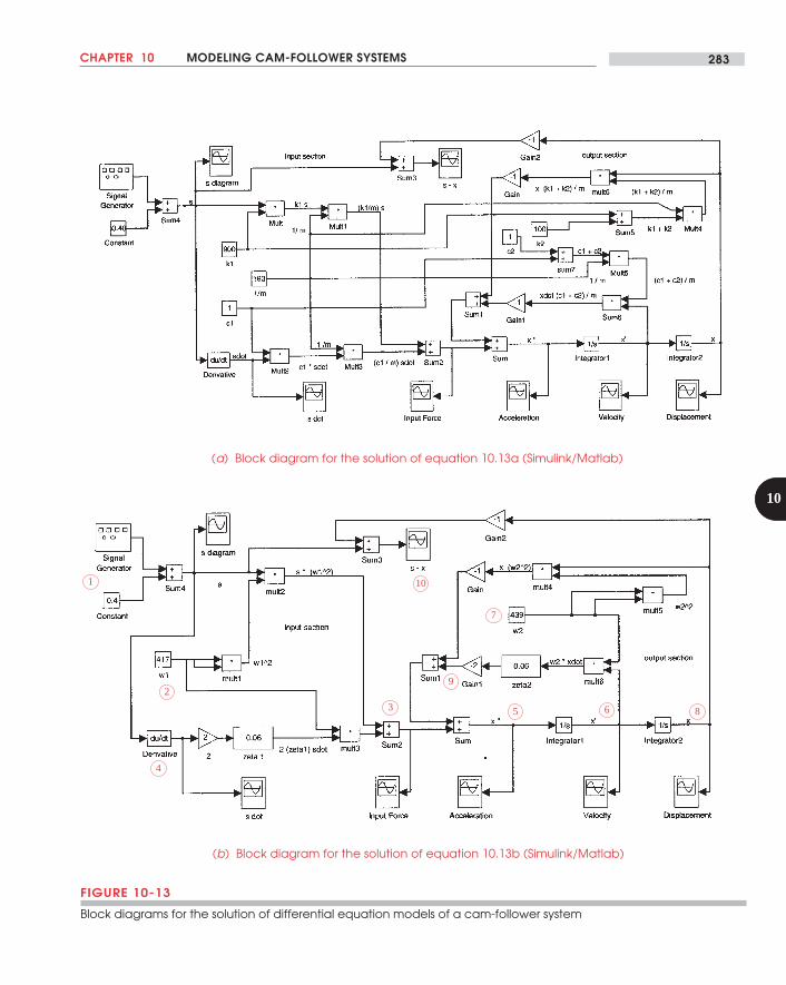
Figure 10-13 shows two such block diagrams, created in SIMULINK . Figure 10-13ais a block diagram for equation 10-13a; it expresses the system motion in terms of thebasic parameters m, k1, k2, c1, and c2. Figure 10-13b shows a block diagram for equa-tion 10-13b; it defines the same system in terms of the natural frequencies ω1, ω2, andthe dimensionless damping ratios ζ1 and ζ2. If one wants to work in terms of the funda-mental parameters of the system rather than normalized values, then Figure 10-13awould be preferred. Both models give identical results when solved numerically.
The block diagram for the normalized equation 10.13b in Figure 10-13b is some-what "cleaner" and so is easier to follow. At point 1 (circled), a signal generator is usedto provide an input function. This SIMULINK icon provides sine, sawtooth, square wave,and random noise functions. A different icon than shown allows the input of a tabulatedfunction that can be the actual displacement and/or velocity data (including dwells) forthe selected cam program, such as modified sine, cycloidal, or a custom spline program,for example.
CHAPTER 10 MODELING CAM-FOLLOWER SYSTEMS 283
10
FIGURE 10-13
Block diagrams for the solution of differential equation models of a cam-follower system
(a) Block diagram for the solution of equation 10.13a (Simulink/Matlab)
(b) Block diagram for the solution of equation 10.13b (Simulink/Matlab)
1
2
3
4
5 6
7
9
8
10
CAM DESIGN AND MANUFACTURING HANDBOOK284
10
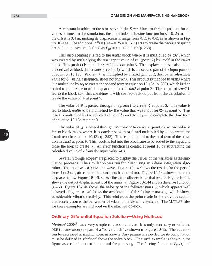
A constant is added to the sine wave in the Sum4 block to force it positive for allvalues of time. In this simulation, the amplitude of the sine function for s is 0. 25 in, andthe offset is 0.4 in, making its displacement range from 0.15 to 0.65 in as shown in Fig-ure 10-14a. The additional offset (0.4 – 0.25 = 0.15 in) acts to create the necessary springpreload on the system, defined as Fpl in equation 9.10 (p. 233).
This displacement s is fed to the mult2 block where it is multiplied by ω12, which
was created by multiplying the user-input value of ω1 (point 2) by itself in the mult1block. This product is fed to the sum2 block at point 3. The displacement s is also fed tothe derivative block that creates s (point 4), which is the second part of the input portionof equation 10.13b. Velocity s is multiplied by a fixed gain of 2, then by an adjustablevalue for ζ1 (using a graphical slider not shown). This product is then fed to mult3 whereit is multiplied by ω1 to create the second term in equation 10.13b (p. 282), which is thenadded to the first term of the equation in block sum2 at point 3. The output of sum2 isfed to the block sum that combines it with the fed-back output from the calculation tocreate the value of ˙x at point 5.
The value of x is passed through integrator1 to create x at point 6. This value isfed to block mult6 to be multiplied by the value that was input for ω2 at point 7. Thisresult is multiplied by the selected value of ζ2 and then by –2 to complete the third termof equation 10.13b at point 9.
The value of x is passed through integrator2 to create x (point 8), whose value isfed to block mult4 where it is combined with ω2
2, and multiplied by –1 to create thefourth term in equation 10.13b (p. 282). This result is added to the third term of the equa-tion in sum1 at point 9. This result is fed into the block sum to be added to the input andclose the loop to create ˙x . An error function is created at point 10 by subtracting thecalculated value of x from the input value of s.
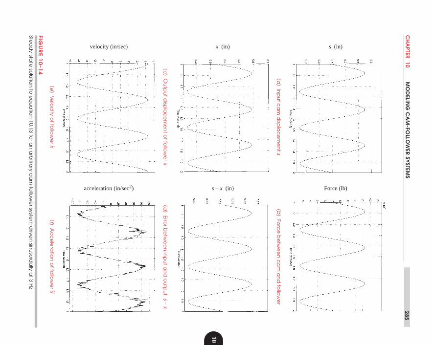
Several "storage scopes" are placed to display the values of the variables as the sim-ulation proceeds. The simulation was run for 2 sec using an Adams integration algo-rithm. The input was a 3 Hz sine wave. Figure 10-14 shows the results for the periodfrom 1 to 2 sec, after the initial transients have died out. Figure 10-14a shows the inputdisplacement s. Figure 10-14b shows the cam-follower force that results. Figure 10-14cshows the output displacement x of the mass m. Figure 10-14d shows the error function(s – x). Figure 10-14e shows the velocity of the follower mass x , which appears wellbehaved. Figure 10-14f shows the acceleration of the follower mass ˙x , which showsconsiderable vibration activity. This reinforces the point made in the previous sectionthat acceleration is the bellwether of vibration in dynamic systems. The MATLAB filesfor these examples are included on the attached CD-ROM.
Ordinary Differential Equation Solution—Using Mathcad
Mathcad 2000® has a very simple-to-use ODE solver. It is only necessary to write theODE (of any order) as part of a "solve block" as shown in Figure 10-15. The equationcan be expressed in implicit form as shown. Any parameters needed for its computationmust be defined in Mathcad above the solve block. One such example is shown in thefigure as a calculation of the natural frequency η1. The forcing functions Vpw(t) and
CH
APTER 10
MO
DELIN
G C
AM
-FOLLO
WER SY
STEMS
285
10
FIGU
RE 1
0-1
4
Stea
dy-sta
te so
lutio
n to
eq
ua
tion
10.13 for a
n a
rbitra
ry ca
m-fo
llow
er syste
m d
riven
sinu
soid
ally a
t 3 Hz
(a) In
pu
t ca
m d
ispla
ce
me
nt s
(b) Fo
rce
be
twe
en
ca
m a
nd
follo
we
r
( c) O
utp
ut d
ispla
ce
me
nt o
f follo
we
r x(d
) Error b
etw
ee
n in
pu
t an
d o
utp
ut s – x
s (in)x (in)velocity (in/sec)
Force (lb)s – x (in)acceleration (in/sec2)
(e) V
elo
city o
f follo
we
r x .(f) A
cc
ele
ratio
n o
f follo
we
r x ..

CAM DESIGN AND MANUFACTURING HANDBOOK286
10
Spw(t), the forcing frequency ω, and the damping ratio ζ were all defined in the Mathcadfile upstream of the solve block, but are not shown in Figure 10-15.
The two initial conditions needed for this second order ODE are then defined, here xand x' at time t = 0 are both set to zero. Then the built-in numerical solver ODESOLVE iscalled and passed values for start time t, end time, tend, and a starting time increment inct.This solver uses a 4th-order Runge-Kutta algorithm with adaptive step size control andplaces the result in the variable R. The solution took only a few seconds to execute on aPentium PC.
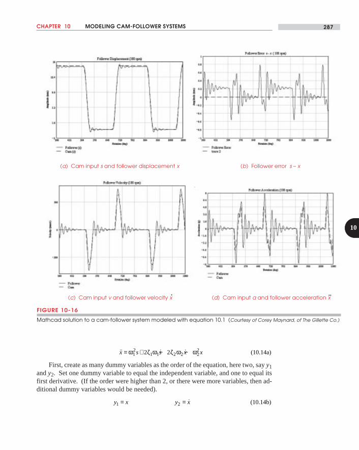
Figure 10-16 shows the result of the Mathcad solution to a cam-follower system runat 180 rpm with the following specifications: Dwell at 15 mm for 150°, modsine fall tozero in 45°, dwell at zero for 120°, and modsine rise to 15 mm in 45°. The follower ef-fective mass is 10 kg, the return spring has k2 = 15 000 N/m and the follower train has k1= 1E6 N/m.
State Space Solutions
Most numerical ODE solver algorithms require that an ODE of order higher than one beconverted to a set of simultaneous first-order ODE's for solution. This is called the statespace form of the system equations. The solver algorithm is structured to do a single nu-merical integration of each equation in the set and iterate until it converges to a solutionat each time step. Most solvers also implement a so-called adaptive step size algorithm.This allows it to take larger steps in regions where the functions are changing slowly andsmaller steps where there is rapid change. This gives more accurate and quicker solutions.For a thorough discussion of the common ODE solver algorithms, see Press et al.[21]
FORCE-CLOSED, ONE-MASS VALVE TRAIN MODEL To put a higher-order ODE intothe state space configuration is a simple process. We will illustrate it first for the force-closed, single-mass system with its return spring at the end effector as shown in Figure10-3a (p. 267). Its equation 10.1b is repeated here, rearranged and renumbered.
FIGURE 10-15
Mathcad solve block to numerically integrate a differential equation
CHAPTER 10 MODELING CAM-FOLLOWER SYSTEMS 287
10
˙ ˙ ˙x s s x x= + − −ω ζ ω ζ ω ω12
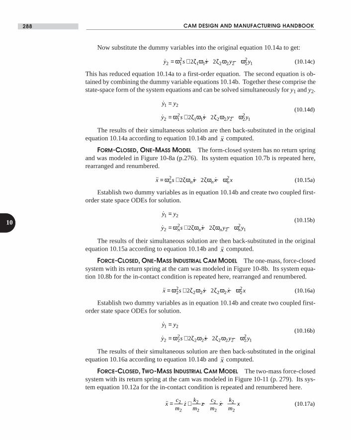
1 1 2 2 222 2 (10.14a)
First, create as many dummy variables as the order of the equation, here two, say y1and y2. Set one dummy variable to equal the independent variable, and one to equal itsfirst derivative. (If the order were higher than 2, or there were more variables, then ad-ditional dummy variables would be needed).
y x y x1 2= = ˙ (10.14b)
FIGURE 10-16
Mathcad solution to a cam-follower system modeled with equation 10.1 (Courtesy of Corey Maynard, of The Gillette Co.)
(c) Cam input v and follower velocity x
(b) Follower error s – x
(d) Cam input a and follower acceleration x
(a) Cam input s and follower displacement x
. ..
CAM DESIGN AND MANUFACTURING HANDBOOK288
10
Now substitute the dummy variables into the original equation 10.14a to get:
˙ ˙y s s y y2 12
1 1 2 2 2 22
12 2= + − −ω ζ ω ζ ω ω (10.14c)
This has reduced equation 10.14a to a first-order equation. The second equation is ob-tained by combining the dummy variable equations 10.14b. Together these comprise thestate-space form of the system equations and can be solved simultaneously for y1 and y2.
˙
˙ ˙
y y
y s s y y
1 2
2 12
1 1 2 2 2 22
12 2
=
= + − −(10.14d)
ω ζ ω ζ ω ω
The results of their simultaneous solution are then back-substituted in the originalequation 10.14a according to equation 10.14b and ˙x computed.
FORM-CLOSED, ONE-MASS MODEL The form-closed system has no return springand was modeled in Figure 10-8a (p.276). Its system equation 10.7b is repeated here,rearranged and renumbered.
˙ ˙ ˙x s s x xn n n n= + − −ω ζω ζω ω2 22 2 (10.15a)
Establish two dummy variables as in equation 10.14b and create two coupled first-order state space ODEs for solution.
˙
˙ ˙
y y
y s s y yn n n n
1 2
22
22
12 2
=
= + − −(10.15b)
ω ζω ζω ω
The results of their simultaneous solution are then back-substituted in the originalequation 10.15a according to equation 10.14b and ˙x computed.
FORCE-CLOSED, ONE-MASS INDUSTRIAL CAM MODEL The one-mass, force-closedsystem with its return spring at the cam was modeled in Figure 10-8b. Its system equa-tion 10.8b for the in-contact condition is repeated here, rearranged and renumbered.
˙ ˙ ˙x s s x x= + − −ω ζ ω ζ ω ω22
2 2 2 2 222 2 (10.16a)
Establish two dummy variables as in equation 10.14b and create two coupled first-order state space ODEs for solution.
˙
˙ ˙
y y
y s s y y
1 2
2 22
2 2 2 2 2 22
12 2
=
= + − −(10.16b)
ω ζ ω ζ ω ω
The results of their simultaneous solution are then back-substituted in the originalequation 10.16a according to equation 10.14b and ˙x computed.
FORCE-CLOSED, TWO-MASS INDUSTRIAL CAM MODEL The two-mass force-closedsystem with its return spring at the cam was modeled in Figure 10-11 (p. 279). Its sys-tem equation 10.12a for the in-contact condition is repeated and renumbered here.
˙ ˙ ˙xc
mz
k
mz
c
mx
k
mx= + − −2
2
2
2
2
2
2
2(10.17a)
CHAPTER 10 MODELING CAM-FOLLOWER SYSTEMS 289
10
Establish two dummy variables as in equation 10.14b and create two coupled first-order state space ODEs for solution.
˙
˙ ˙
y y
yc
mz
k
mz
c
my
k
my
1 2
22
2
2
2
2
22
2
21
=
= + − −
(10.17b)
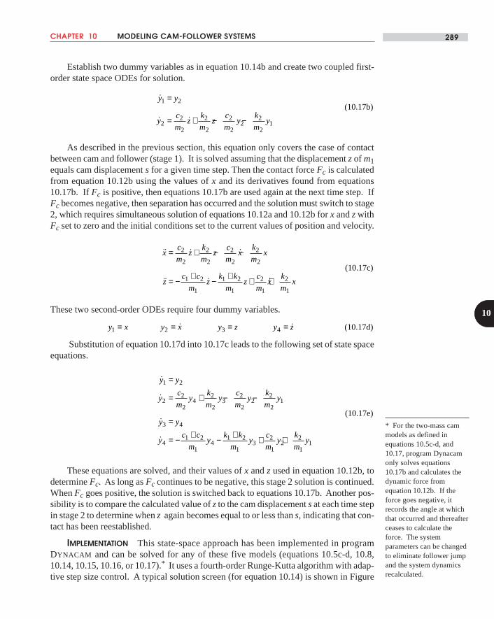
As described in the previous section, this equation only covers the case of contactbetween cam and follower (stage 1). It is solved assuming that the displacement z of m1equals cam displacement s for a given time step. Then the contact force Fc is calculatedfrom equation 10.12b using the values of x and its derivatives found from equations10.17b. If Fc is positive, then equations 10.17b are used again at the next time step. IfFc becomes negative, then separation has occurred and the solution must switch to stage2, which requires simultaneous solution of equations 10.12a and 10.12b for x and z withFc set to zero and the initial conditions set to the current values of position and velocity.
˙ ˙ ˙
˙ ˙ ˙
xc
mz
k
mz
c
mx
k
mx
zc c
mz
k k
mz
c
mx
k
mx
= + − −
= − + − + + +
2
2
2
2
2
2
2
2
1 2
1
1 2
1
2
1
2
1
(10.17c)
These two second-order ODEs require four dummy variables.
y x y x y z y z1 2 3 4= = = =˙ ˙ (10.17d)
Substitution of equation 10.17d into 10.17c leads to the following set of state spaceequations.
˙
˙
˙
˙
y y
yc
my
k
my
c
my
k
my
y y
yc c
my
k k
my
c
my
k
my
1 2
22
24
2
23
2
22
2
21
3 4
41 2
14
1 2
13
2
12
2
11
=
= + − −
=
= − + − + + +
(10.17e)
These equations are solved, and their values of x and z used in equation 10.12b, todetermine Fc. As long as Fc continues to be negative, this stage 2 solution is continued.When Fc goes positive, the solution is switched back to equations 10.17b. Another pos-sibility is to compare the calculated value of z to the cam displacement s at each time stepin stage 2 to determine when z again becomes equal to or less than s, indicating that con-tact has been reestablished.
IMPLEMENTATION This state-space approach has been implemented in programDYNACAM and can be solved for any of these five models (equations 10.5c-d, 10.8,10.14, 10.15, 10.16, or 10.17).* It uses a fourth-order Runge-Kutta algorithm with adap-tive step size control. A typical solution screen (for equation 10.14) is shown in Figure
* For the two-mass cammodels as defined inequations 10.5c-d, and10.17, program Dynacamonly solves equations10.17b and calculates thedynamic force fromequation 10.12b. If theforce goes negative, itrecords the angle at whichthat occurred and thereafterceases to calculate theforce. The systemparameters can be changedto eliminate follower jumpand the system dynamicsrecalculated.
CAM DESIGN AND MANUFACTURING HANDBOOK290
10
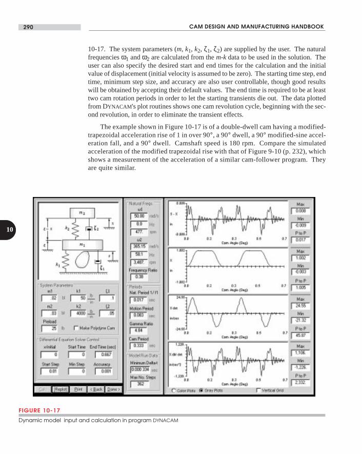
10-17. The system parameters (m, k1, k2, ζ1, ζ2) are supplied by the user. The naturalfrequencies ω1 and ω2 are calculated from the m-k data to be used in the solution. Theuser can also specify the desired start and end times for the calculation and the initialvalue of displacement (initial velocity is assumed to be zero). The starting time step, endtime, minimum step size, and accuracy are also user controllable, though good resultswill be obtained by accepting their default values. The end time is required to be at leasttwo cam rotation periods in order to let the starting transients die out. The data plottedfrom DYNACAM 's plot routines shows one cam revolution cycle, beginning with the sec-ond revolution, in order to eliminate the transient effects.
The example shown in Figure 10-17 is of a double-dwell cam having a modified-trapezoidal acceleration rise of 1 in over 90°, a 90° dwell, a 90° modified-sine accel-eration fall, and a 90° dwell. Camshaft speed is 180 rpm. Compare the simulatedacceleration of the modified trapezoidal rise with that of Figure 9-10 (p. 232), whichshows a measurement of the acceleration of a similar cam-follower program. Theyare quite similar.
FIGURE 10-17
Dynamic model input and calculation in program DYNACAM
CHAPTER 10 MODELING CAM-FOLLOWER SYSTEMS 291
10
10.8 POLYDYNE CAM FUNCTIONS
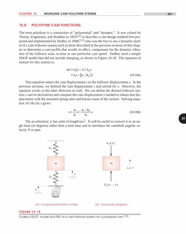
The term polydyne is a contraction of "polynomial" and "dynamic." It was coined byThoren, Engemann, and Stoddart in 1953[12] to describe a cam design method first pro-posed and implemented by Dudley in 1948,[13] who was the first to use a dynamic mod-el of a cam-follower system such as those described in the previous sections of this chap-ter to determine a cam profile that would, in effect, compensate for the dynamic vibra-tion of the follower train, at least at one particular cam speed. Dudley used a simpleSDOF model that did not include damping, as shown in Figure 10-18. The equation ofmotion for this system is:
mx k s x k x
k s k k x
˙ = −( ) −
= − +( )1 2
1 1 2 (10.18a)
This equation relates the cam displacement s to the follower displacement x. In theprevious sections, we defined the cam displacement s and solved for x. However, theequation works in the other direction as well. We can define the desired follower mo-tion x and its derivatives and compute the cam displacement s needed to obtain that dis-placement with the assumed spring rates and known mass of the system. Solving equa-tion 10.18a for s gives:
sm
kx
k k
kx= + +
1
1 2
1
˙ (10.18b)
The acceleration x has units of length/sec2. It will be useful to convert it to an an-gle base (in degrees) rather than a time base and to introduce the camshaft angular ve-locity N in rpm.
FIGURE 10-18
Dudley's SDOF model and FBD of a cam-follower system for a polydyne cam [13]
(b) Free-body diagram
m
k1(s – x)
k2(x)
(a) Lumped parameter model
x
m
s, x +
k1
k2
s

CAM DESIGN AND MANUFACTURING HANDBOOK292
10
length
sec
length
deg
360 deg
rev
rev
60 sec
(10.19)
2 2
2 2
2
2
2 2=
= =
N
xd x
dtN
d x
d
2
2
22
2
236˙θ
Substitute equation 10.19 in 10.18b.
s Nm
k
d x
d
k k
kx=
+ +
36 2
1
2
21 2
1θ(10.20a)
Differentiate with respect to θ to get the polydyne cam velocity function.
s Nm
k
d x
d
k k
k
dx
d=
+ +
36 2
1
3
31 2
1θ θ(10.20b)
Differentiate again with respect to θ to get the polydyne cam acceleration function.
˙s Nm
k
d x
d
k k
k
d x
d=
+ +
36 2
1
4
41 2
1
2
2θ θ(10.20c)
Note that the cam acceleration function involves the fourth derivative of the select-ed follower displacement function, which we call "ping." This means that any functionselected for the follower displacement must be continuous through at least four deriva-tives, velocity, acceleration, jerk, and ping. Since polynomial functions allow control ofcontinuity at the ends of the segment to any derivative, they provide a useful means tothis end. Spline functions can also satisfy these requirements.
Dudley's polydyne model of Figure 10-18 is for a system with the return spring act-ing at the end effector. For an industrial cam that has the return spring acting on the camshoe, the model of Figure 10-8 is more appropriate. If we assume that contact is main-tained between cam and follower and that damping is negligible, we can write the sys-tem equation as a modification of equation 10.7, leaving out the damping terms.
˙xk
mx
k
ms+ = (10.21a)
Rearrange to solve for s:
sm
kx x= +˙ (10.21b)
Substitute equation 10.19 in 10.21b
s Nm
k
d x
dx= +36 2
2
2θ(10.22a)
Differentiate with respect to θ to get the polydyne cam velocity function.
s Nm
k
d x
d
dx
d= +36 2
3
3θ θ(10.22b)
CHAPTER 10 MODELING CAM-FOLLOWER SYSTEMS 293
10
Differentiate again with respect to θ to get the polydyne cam acceleration function.
˙s Nm
k
d x
d
d x
d= +36 2
4
4
2
2θ θ(10.22c)
Note the presence of cam speed N in equations 10.20 and 10.22. For any selectedfollower function x and its derivatives, the cam profile, as defined by the function s (equa-tion 10.20a or 10.22a) will be different for any value of N selected. This means that thedynamic behavior of the system can be optimized (i.e, vibration minimized) only for oneoperating speed. If the system will be operated at a single speed, this is not a problem. Ifnot, then one speed in its range will have to be selected for the cam profile definition andthe system will have some vibration when operated at any other speed. When applied toengine valve trains that obviously operate over a wide range of speeds, a speed close tothe highest expected operating speed is typically used in equations 10.20. Fawcett and Fawc-ett[20] show that a polydyne cam will always give lower vibration than a non-polydyne camhaving the same follower program when its speed is greater than 0.707N. They also state that:
By a suitable choice of N, the speeds at which a polydyne cam is inferior may berelegated to the lower part of the speed range of the mechanism where (the inherentlylower, ed.) vibration amplitudes are not a problem.
Given an effective dynamic model of the system as described by equation 10.18a,the problem devolves to identifying one or more suitable polynomial functions for x thatprovide sufficient control of continuity and that also yield acceptable peak values of ve-locity and acceleration of the follower for any given set of kinematic constraints on thefollower motion. However, Dudley points out that:
With a flexible valve linkage, one must accept higher accelerations at the valve(follower) than would occur with a rigid connecting system. There is a corollary: Ifa cam is designed on the assumption of a rigid system, the actual limiting speed willbe appreciably lower than the theoretical value.
The derivations of these polydyne polynomials are long and involved and will notbe reproduced here. The interested reader can explore them in the original references giv-en. Dudley addressed the problem of valve cam design for the overhead valve-pushrodcam-follower system as shown in Figure 10-1, which is a relatively soft system and canhave significant vibration problems. In valve trains, it also is necessary to maximize thearea under the valve lift curve since it directly affects engine breathing. Dudley includedthis constraint in his development of the equations. He also attempted to minimize peakaccelerations and to have an acceleration curve not dissimilar in shape to those that hadproven successful in the past Some trial and error was involved, particularly in respectto choice of powers to be used in the x equation. He determined that a polynomial equa-tion of this form was suitable.
s h C C C Cp
p
q
p
r
p
= +
+
+
+
+ +
1 2
2 2 4θβ
θβ
θβ
θβ
(10.23a)
where the constants are defined by:
CAM DESIGN AND MANUFACTURING HANDBOOK294
10
Cp p
p p2
2
26 24
6 8 8= − −
− −(10.23b)
Cp p p
p pp = + + +
− −
3 2
27 14 8
6 8 8(10.23c)
Cp p p
p pq = − − +
− −2 4 16
6 8 8
3 2
2 (10.23d)
Cp p p
p pr = − +
− −
3 2
23 2
6 8 8(10.23e)
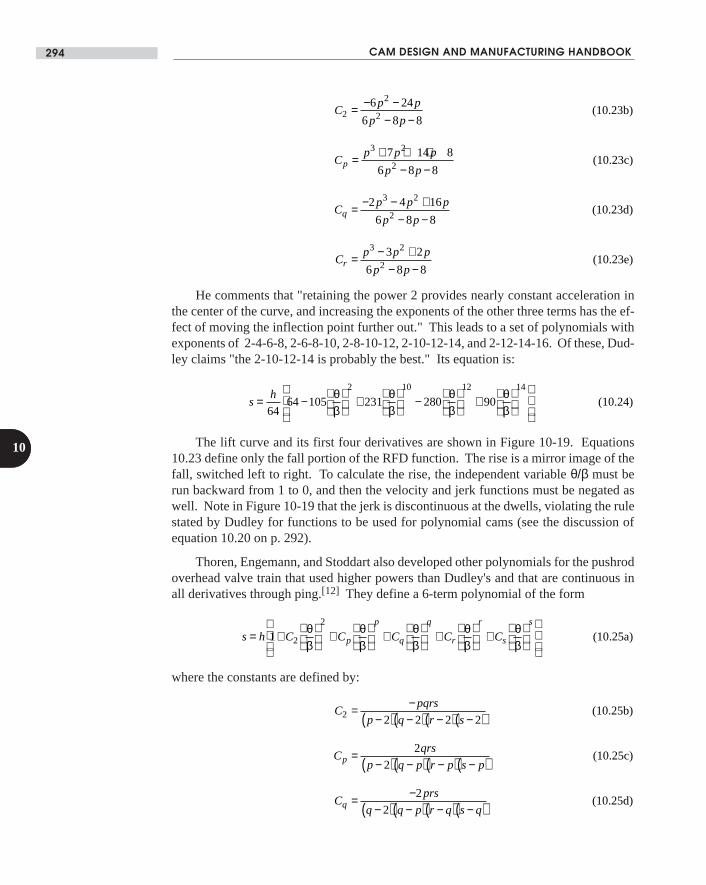
He comments that "retaining the power 2 provides nearly constant acceleration inthe center of the curve, and increasing the exponents of the other three terms has the ef-fect of moving the inflection point further out." This leads to a set of polynomials withexponents of 2-4-6-8, 2-6-8-10, 2-8-10-12, 2-10-12-14, and 2-12-14-16. Of these, Dud-ley claims "the 2-10-12-14 is probably the best." Its equation is:
sh= −
+
−
+
64
64 105 231 280 902 10 12 14
θβ
θβ
θβ
θβ
(10.24)
The lift curve and its first four derivatives are shown in Figure 10-19. Equations10.23 define only the fall portion of the RFD function. The rise is a mirror image of thefall, switched left to right. To calculate the rise, the independent variable θ/β must berun backward from 1 to 0, and then the velocity and jerk functions must be negated aswell. Note in Figure 10-19 that the jerk is discontinuous at the dwells, violating the rulestated by Dudley for functions to be used for polynomial cams (see the discussion ofequation 10.20 on p. 292).
Thoren, Engemann, and Stoddart also developed other polynomials for the pushrodoverhead valve train that used higher powers than Dudley's and that are continuous inall derivatives through ping.[12] They define a 6-term polynomial of the form
s h C C C C Cp
p
q
q
r
r
s
s
= +
+
+
+
+
1 2
2θβ
θβ
θβ
θβ
θβ
(10.25a)
where the constants are defined by:
Cpqrs
p q r s2 2 2 2 2= −
−( ) −( ) −( ) −( )(10.25b)
Cqrs
p q p r p s pp =−( ) −( ) −( ) −( )
2
2(10.25c)
Cprs
q q p r q s qq = −−( ) −( ) −( ) −( )
2
2(10.25d)
CHAPTER 10 MODELING CAM-FOLLOWER SYSTEMS 295
10
0
1.8
0
0
0
–1.8
8.0
–8.0
105
–105
969
–969
0
1
βrise βfall
Displac.
Velocity
Accel.
Jerk
Ping
βθ
2 2
2h
d x
d
x
h
βθ
3 3
3h
d x
d
βθh
dx
d
βθ
4 4
4h
d x
d
θ
θ
θ
θ
θ
FIGURE 10-19
A 2-10-12-14 polynomial rise-return follower function for a polydyne valve cam
Cpqs
r r p r q s rr =−( ) −( ) −( ) −( )
2
2(10.25e)
Cpqr
s s p s q s rs = −−( ) −( ) −( ) −( )
2
2(10.25f)
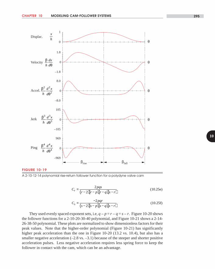
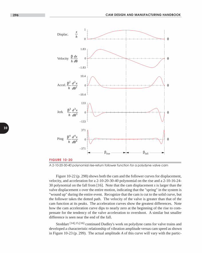
They used evenly spaced exponent sets, i.e, q – p = r – q = s– r. Figure 10-20 showsthe follower functions for a 2-10-20-30-40 polynomial, and Figure 10-21 shows a 2-14-26-38-50 polynomial. These plots are normalized to show dimensionless factors for theirpeak values. Note that the higher-order polynomial (Figure 10-21) has significantlyhigher peak acceleration than the one in Figure 10-20 (13.2 vs. 10.4), but also has asmaller negative acceleration (–2.8 vs. –3.1) because of the steeper and shorter positiveacceleration pulses. Less negative acceleration requires less spring force to keep thefollower in contact with the cam, which can be an advantage.
CAM DESIGN AND MANUFACTURING HANDBOOK296
10
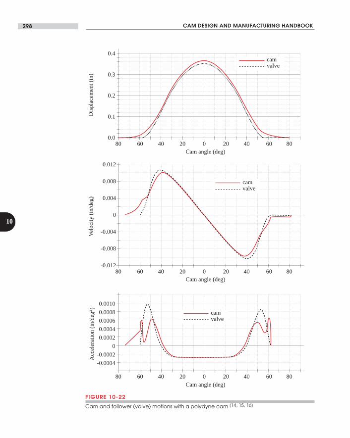
Figure 10-22 (p. 298) shows both the cam and the follower curves for displacement,velocity, and acceleration for a 2-10-20-30-40 polynomial on the rise and a 2-10-16-24-30 polynomial on the fall from [16]. Note that the cam displacement s is larger than thevalve displacement x over the entire motion, indicating that the "spring" in the system is"wound up" during the entire event. Recognize that the cam is cut to the solid curve, butthe follower takes the dotted path. The velocity of the valve is greater than that of thecam function at its peaks. The acceleration curves show the greatest differences. Notehow the cam acceleration curve dips to nearly zero at the beginning of the rise to com-pensate for the tendency of the valve acceleration to overshoot. A similar but smallerdifference is seen near the end of the fall.
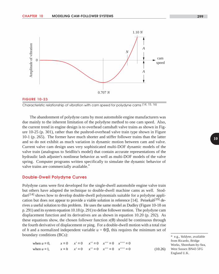
Stoddart [14],15,[16] continued Dudley's work on polydyne cams for valve trains anddeveloped a characteristic relationship of vibration amplitude versus cam speed as shownin Figure 10-23 (p. 299). The actual amplitude A of this curve will vary with the partic-
0
1.83
0
0
0
–1.83
10.4
–10.4
133
–133
371
–371
0
1
βrise βfall
Displac.
Velocity
Accel.
Jerk
Ping
βθ
2 2
2h
d x
d
x
h
βθ
3 3
3h
d x
d
βθh
dx
d
βθ
4 4
4h
d x
d
θ
θ
θ
θ
θ
FIGURE 10-20
A 2-10-20-30-40 polynomial rise-return follower function for a polydyne valve cam
CHAPTER 10 MODELING CAM-FOLLOWER SYSTEMS 297
10
0
1.85
0
0
0
–1.85
13.2
–13.2
220
–220
810
–810
0
1
βrise βfall
Displac.
Velocity
Accel.
Jerk
Ping
βθ
2 2
2h
d x
d
x
h
βθ
3 3
3h
d x
d
βθh
dx
d
βθ
4 4
4h
d x
d
θ
θ
θ
θ
θ
FIGURE 10-21
A 2-14-26-38-50 polynomial rise-return follower function for a polydyne valve cam
ular follower train, but the shape will be similar in all cases. The sign of A is not of inter-est since the direction of vibration is not relevant, only its magnitude. Note that the vi-bration amplitude is zero at the design speed N, peaks at 0.707N, and reaches the samelevel A at 1.1N, increasing rapidly at higher speeds.
Polydyne functions were used extensively for automotive valve cams in the U. S. inthe 1950's and 1960's, but they have not been used in these applications in recent years.Instead, spline functions are now more commonly used for valve trains. Figure 10-24shows a modern spline-function design for a single overhead camshaft (SOHC) valvetrain.[17] Note the asymmetry of the acceleration function, a design freedom allowed bythe use of spline functions. This design uses a quartic spline for displacement, but isdesigned from the acceleration using designer-shaped quadratic splines.[18] The stepfunctions in the acceleration function before and after the lift event are the opening andclosing ramps used to wind up the system compliance.[17]
CAM DESIGN AND MANUFACTURING HANDBOOK298
10
Acc
eler
atio
n (in
/deg2
)
Cam angle (deg)0 20 40 60 8020406080
0.0
0.1
0.2
0.3
0.4
Dis
plac
emen
t (in
)
Cam angle (deg)0 20 40 60 8020406080
Velo
city
(in
/deg
)
Cam angle (deg)0 20 40 60 8020406080
0
-0.004
-0.008
-0.012
0.012
0.008
0.004
0
-0.0002
-0.0004
0.0010
0.0006
0.0004
0.0008
0.0002
FIGURE 10-22
Cam and follower (valve) motions with a polydyne cam [14, 15, 16]
camvalve
camvalve
camvalve
CHAPTER 10 MODELING CAM-FOLLOWER SYSTEMS 299
10
FIGURE 10-23
Characteristic relationship of vibration with cam speed for polydyne cams [14, 15, 16]
1.10 N
0.707 N
Am
plitu
de o
f vib
ratio
n
0 cam speed
A
AN
The abandonment of polydyne cams by most automobile engine manufacturers wasdue mainly to the inherent limitation of the polydyne method to one cam speed. Also,the current trend in engine design is to overhead camshaft valve trains as shown in Fig-ure 10-25 (p. 301), rather than the pushrod-overhead valve train type shown in Figure10-1 (p. 265). The former have much shorter and stiffer follower trains than the latterand so do not exhibit as much variation in dynamic motion between cam and valve.Current valve cam design uses very sophisticated multi-DOF dynamic models of thevalve train (analogous to Seidlitz's model) that contain accurate representations of thehydraulic lash adjuster's nonlinear behavior as well as multi-DOF models of the valvespring. Computer programs written specifically to simulate the dynamic behavior ofvalve trains are commercially available.*
Double-Dwell Polydyne Curves
Polydyne cams were first developed for the single-dwell automobile engine valve trainbut others have adapted the technique to double-dwell machine cams as well. Stod-dart[14] shows how to develop double-dwell polynomials suitable for a polydyne appli-cation but does not appear to provide a viable solution in reference [14]. Peisekah[19] de-rives a useful solution to this problem. He uses the same model as Dudley (Figure 10-18 onp. 291) and its system equation 10.18 (p. 291) to define follower motion. The polydyne camdisplacement function and its derivatives are as shown in equation 10.20 (p. 292). Asthese equations show, the chosen follower function x(θ) should be continuous throughthe fourth derivative of displacement or ping. For a double-dwell motion with a total riseof h and a normalized independent variable u = θ/β, this requires the minimum set ofboundary conditions (BCs):
when
when (10.26)
u x x x x x
u x h x x x x
= = ′ = ′′ = ′′′ = ′′′′ == = ′ = ′′ = ′′′ = ′′′′ =
0 0 0 0 0 0
1 0 0 0 0
,
,
* e.g., Valdyne, availablefrom Ricardo, BridgeWorks, Shoreham-by-Sea,West Sussex BN43 5FGEngland U.K.
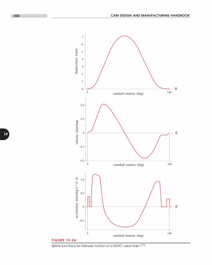
CAM DESIGN AND MANUFACTURING HANDBOOK300
10
disp
lace
men
t (m
m)
camshaft rotation (deg)
0
1
0 140
2
3
4
5
6
7
velo
city
(m
m/d
eg)
camshaft rotation (deg)
0
0.1
–0.2
–0.1
0 140
0.2
acce
lera
tion
(m
m/d
eg^2
* E
–2)
camshaft rotation (deg)
0
0.5
1.0
–0.5
0 140
θ
θ
θ
FIGURE 10-24
Spline functions for follower motion of a SOHC valve train [17]
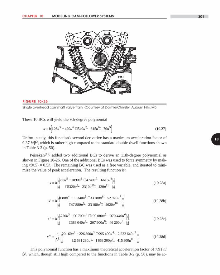
CHAPTER 10 MODELING CAM-FOLLOWER SYSTEMS 301
10
These 10 BCs will yield the 9th-degree polynomial
x h u u u u u= − + − +[ ]126 420 540 315 705 6 7 8 9 (10.27)
Unfortunately, this function's second derivative has a maximum acceleration factor of9.37 h/β2, which is rather high compared to the standard double-dwell functions shownin Table 3-2 (p. 50).
Peisekah[19] added two additional BCs to derive an 11th-degree polynomial asshown in Figure 10-26. One of the additional BCs was used to force symmetry by mak-ing x(0.5) = 0.5h. The remaining BC was used as a free variable, and iterated to mini-mize the value of peak acceleration. The resulting function is:
x hu u u u
u u u=
− + −
+ − +
336 1890 4740 6615
5320 2310 420
5 6 7 8
9 10 11(10.28a)
′ =− + −
+ − +
x hu u u u
u u u
1680 11 340 33180 52 920
47 880 23100 4620
4 5 6 7
8 9 10(10.28b)
′′ =− + −
+ − +
x hu u u u
u u u
6720 56 700 199 080 370 440
383 040 207 900 46 200
3 4 5 6
7 8 9(10.28c)
′′′ =− + −
+ − +
xh u u u u
u u uβ3
2 3 4 5
6 7 8
20 160 226 800 995 400 2 222 640
2 681 280 1 663 200 415 800(10.28d)
This polynomial function has a maximum theoretical acceleration factor of 7.91 h/β2, which, though still high compared to the functions in Table 3-2 (p. 50), may be ac-
FIGURE 10-25
Single overhead camshaft valve train (Courtesy of DaimlerChrysler, Auburn Hills, MI)
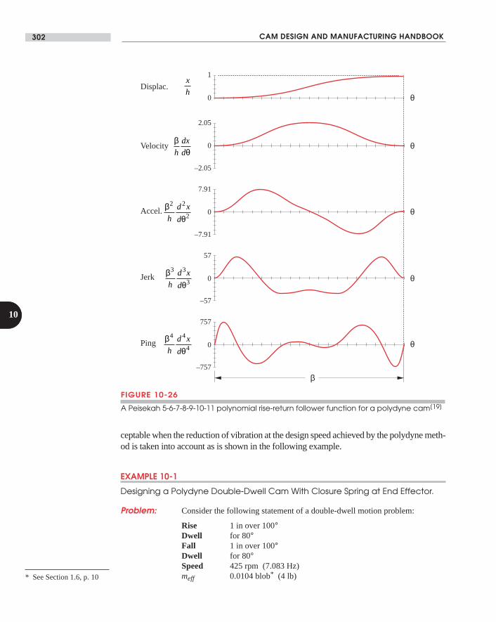
CAM DESIGN AND MANUFACTURING HANDBOOK302
10
ceptable when the reduction of vibration at the design speed achieved by the polydyne meth-od is taken into account as is shown in the following example.
EXAMPLE 10-1
Designing a Polydyne Double-Dwell Cam With Closure Spring at End Effector.
Problem: Consider the following statement of a double-dwell motion problem:
Rise 1 in over 100°Dwell for 80°Fall 1 in over 100°Dwell for 80°Speed 425 rpm (7.083 Hz)meff 0.0104 blob* (4 lb)
0
2.05
0
0
0
–2.05
7.91
–7.91
57
–57
757
–757
0
1
β
Displac.
Velocity
Accel.
Jerk
Ping
βθ
2 2
2h
d x
d
x
h
βθ
3 3
3h
d x
d
βθh
dx
d
βθ
4 4
4h
d x
d
θ
θ
θ
θ
θ
FIGURE 10-26
A Peisekah 5-6-7-8-9-10-11 polynomial rise-return follower function for a polydyne cam[19]
* See Section 1.6, p. 10
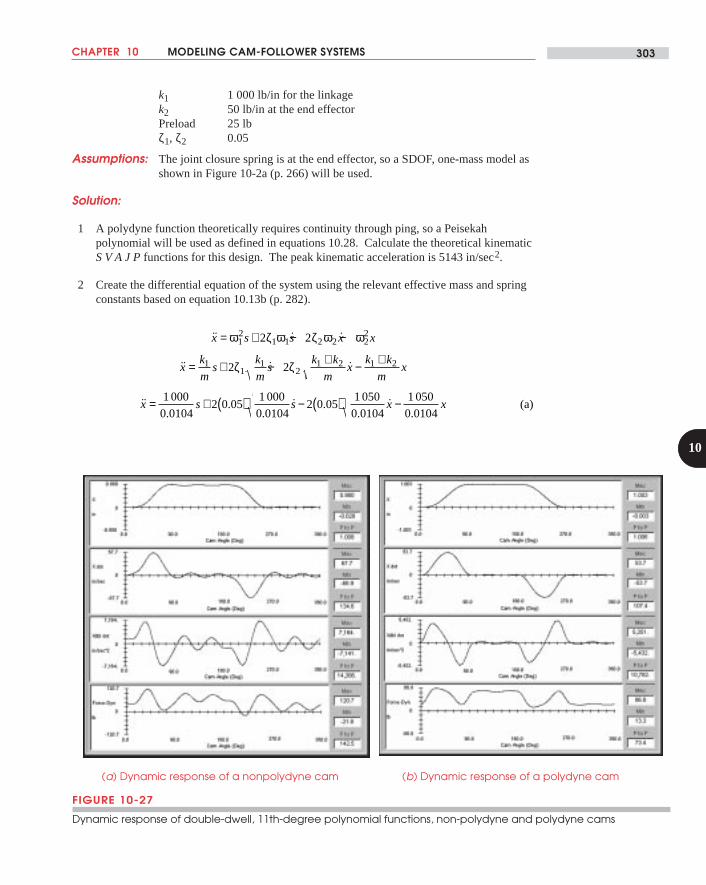
CHAPTER 10 MODELING CAM-FOLLOWER SYSTEMS 303
10
k1 1 000 lb/in for the linkagek2 50 lb/in at the end effectorPreload 25 lbζ1, ζ2 0.05
Assumptions: The joint closure spring is at the end effector, so a SDOF, one-mass model asshown in Figure 10-2a (p. 266) will be used.
Solution:
1 A polydyne function theoretically requires continuity through ping, so a Peisekahpolynomial will be used as defined in equations 10.28. Calculate the theoretical kinematicS V A J P functions for this design. The peak kinematic acceleration is 5143 in/sec2.
2 Create the differential equation of the system using the relevant effective mass and springconstants based on equation 10.13b (p. 282).
˙ ˙ ˙
˙ ˙ ˙
˙.
..
˙ ..
˙.
x s s x x
xk
ms
k
ms
k k
mx
k k
mx
x s s x x
= + − −
= + − + − +
= + ( ) − ( ) −
ω ζ ω ζ ω ω
ζ ζ
12
1 1 2 2 22
11
12
1 2 1 2
2 2
2 2
1 000
0 01042 0 05
1 000
0 01042 0 05
1 050
0 0104
1 050
0 0104(a)
FIGURE 10-27
Dynamic response of double-dwell, 11th-degree polynomial functions, non-polydyne and polydyne cams
(a) Dynamic response of a nonpolydyne cam (b) Dynamic response of a polydyne cam
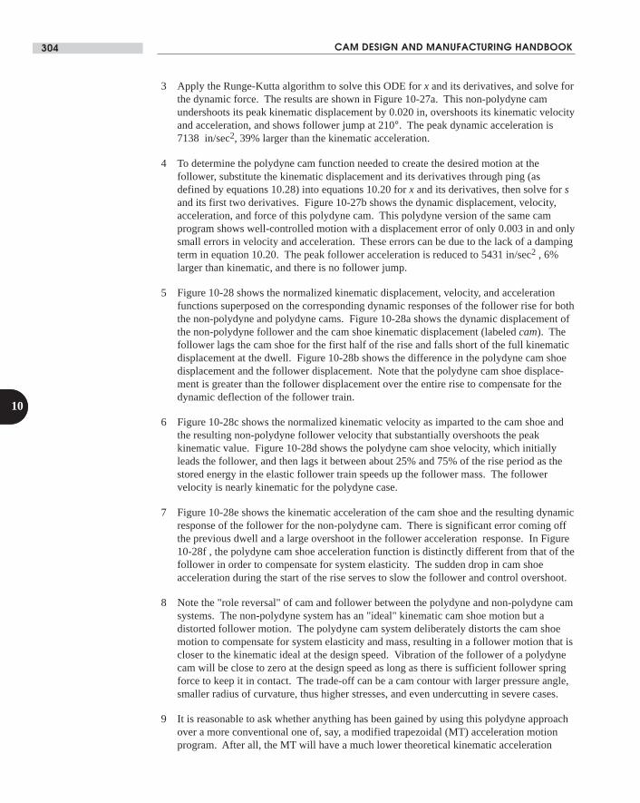
CAM DESIGN AND MANUFACTURING HANDBOOK304
10
3 Apply the Runge-Kutta algorithm to solve this ODE for x and its derivatives, and solve forthe dynamic force. The results are shown in Figure 10-27a. This non-polydyne camundershoots its peak kinematic displacement by 0.020 in, overshoots its kinematic velocityand acceleration, and shows follower jump at 210°. The peak dynamic acceleration is7138 in/sec2, 39% larger than the kinematic acceleration.
4 To determine the polydyne cam function needed to create the desired motion at thefollower, substitute the kinematic displacement and its derivatives through ping (asdefined by equations 10.28) into equations 10.20 for x and its derivatives, then solve for sand its first two derivatives. Figure 10-27b shows the dynamic displacement, velocity,acceleration, and force of this polydyne cam. This polydyne version of the same camprogram shows well-controlled motion with a displacement error of only 0.003 in and onlysmall errors in velocity and acceleration. These errors can be due to the lack of a dampingterm in equation 10.20. The peak follower acceleration is reduced to 5431 in/sec2 , 6%larger than kinematic, and there is no follower jump.
5 Figure 10-28 shows the normalized kinematic displacement, velocity, and accelerationfunctions superposed on the corresponding dynamic responses of the follower rise for boththe non-polydyne and polydyne cams. Figure 10-28a shows the dynamic displacement ofthe non-polydyne follower and the cam shoe kinematic displacement (labeled cam). Thefollower lags the cam shoe for the first half of the rise and falls short of the full kinematicdisplacement at the dwell. Figure 10-28b shows the difference in the polydyne cam shoedisplacement and the follower displacement. Note that the polydyne cam shoe displace-ment is greater than the follower displacement over the entire rise to compensate for thedynamic deflection of the follower train.
6 Figure 10-28c shows the normalized kinematic velocity as imparted to the cam shoe andthe resulting non-polydyne follower velocity that substantially overshoots the peakkinematic value. Figure 10-28d shows the polydyne cam shoe velocity, which initiallyleads the follower, and then lags it between about 25% and 75% of the rise period as thestored energy in the elastic follower train speeds up the follower mass. The followervelocity is nearly kinematic for the polydyne case.
7 Figure 10-28e shows the kinematic acceleration of the cam shoe and the resulting dynamicresponse of the follower for the non-polydyne cam. There is significant error coming offthe previous dwell and a large overshoot in the follower acceleration response. In Figure10-28f , the polydyne cam shoe acceleration function is distinctly different from that of thefollower in order to compensate for system elasticity. The sudden drop in cam shoeacceleration during the start of the rise serves to slow the follower and control overshoot.
8 Note the "role reversal" of cam and follower between the polydyne and non-polydyne camsystems. The non-polydyne system has an "ideal" kinematic cam shoe motion but adistorted follower motion. The polydyne cam system deliberately distorts the cam shoemotion to compensate for system elasticity and mass, resulting in a follower motion that iscloser to the kinematic ideal at the design speed. Vibration of the follower of a polydynecam will be close to zero at the design speed as long as there is sufficient follower springforce to keep it in contact. The trade-off can be a cam contour with larger pressure angle,smaller radius of curvature, thus higher stresses, and even undercutting in severe cases.
9 It is reasonable to ask whether anything has been gained by using this polydyne approachover a more conventional one of, say, a modified trapezoidal (MT) acceleration motionprogram. After all, the MT will have a much lower theoretical kinematic acceleration
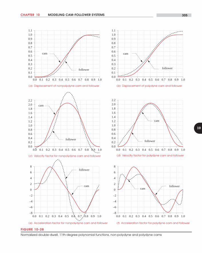
CHAPTER 10 MODELING CAM-FOLLOWER SYSTEMS 305
10
–8
–4
0
4
6
–6
–2
2
8
0.0
0.4
0.8
1.2
1.6
2.0
0.2
0.6
1.0
1.4
1.8
2.2
0.0 0.1 0.2 0.3 0.4 0.5 0.6 0.7 0.8 0.9 1.0
cam
follower
0.0
0.2
0.4
0.6
0.8
1.0
0.1
0.3
0.5
0.7
0.9
1.1
0.0 0.1 0.2 0.3 0.4 0.5 0.6 0.7 0.8 0.9 1.0
follower
cam
(a) Displacement of nonpolydyne cam and follower (b) Displacement of polydyne cam and follower
0.0
0.2
0.4
0.6
0.8
1.0
0.1
0.3
0.5
0.7
0.9
1.1
0.0 0.1 0.2 0.3 0.4 0.5 0.6 0.7 0.8 0.9 1.0
follower
cam
0.0 0.1 0.2 0.3 0.4 0.5 0.6 0.7 0.8 0.9 1.0
follower
cam
FIGURE 10-28
Normalized double-dwell, 11th-degree polynomial functions, non-polydyne and polydyne cams
(e) Acceleration factor for nonpolydyne cam and follower (f) Acceleration factor for polydyne cam and follower
(d) Velocity factor for polydyne cam and follower
–8
–4
0
4
6
–6
–2
2
8
0.0 0.1 0.2 0.3 0.4 0.5 0.6 0.7 0.8 0.9 1.0
camfollower
0.0
0.4
0.8
1.2
1.6
2.0
0.2
0.6
1.0
1.4
1.8
2.2
0.0 0.1 0.2 0.3 0.4 0.5 0.6 0.7 0.8 0.9 1.0
follower
cam
(c) Velocity factor for nonpolydyne cam and follower
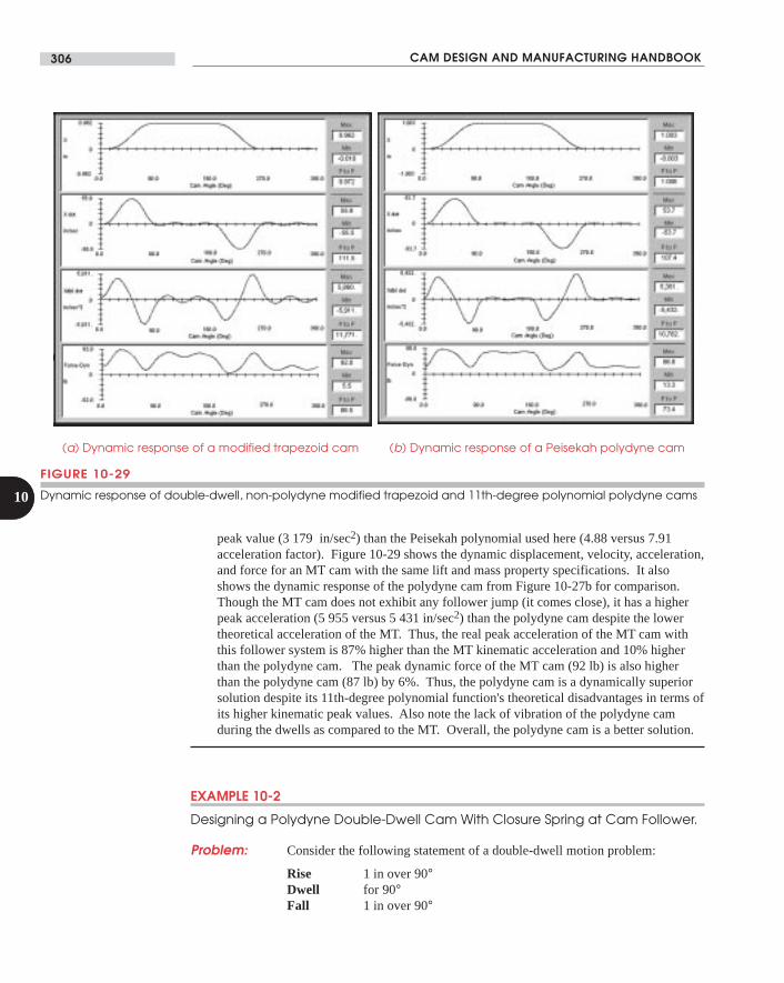
CAM DESIGN AND MANUFACTURING HANDBOOK306
10
FIGURE 10-29
Dynamic response of double-dwell, non-polydyne modified trapezoid and 11th-degree polynomial polydyne cams
(a) Dynamic response of a modified trapezoid cam (b) Dynamic response of a Peisekah polydyne cam
peak value (3 179 in/sec2) than the Peisekah polynomial used here (4.88 versus 7.91acceleration factor). Figure 10-29 shows the dynamic displacement, velocity, acceleration,and force for an MT cam with the same lift and mass property specifications. It alsoshows the dynamic response of the polydyne cam from Figure 10-27b for comparison.Though the MT cam does not exhibit any follower jump (it comes close), it has a higherpeak acceleration (5 955 versus 5 431 in/sec2) than the polydyne cam despite the lowertheoretical acceleration of the MT. Thus, the real peak acceleration of the MT cam withthis follower system is 87% higher than the MT kinematic acceleration and 10% higherthan the polydyne cam. The peak dynamic force of the MT cam (92 lb) is also higherthan the polydyne cam (87 lb) by 6%. Thus, the polydyne cam is a dynamically superiorsolution despite its 11th-degree polynomial function's theoretical disadvantages in terms ofits higher kinematic peak values. Also note the lack of vibration of the polydyne camduring the dwells as compared to the MT. Overall, the polydyne cam is a better solution.
EXAMPLE 10-2
Designing a Polydyne Double-Dwell Cam With Closure Spring at Cam Follower.
Problem: Consider the following statement of a double-dwell motion problem:
Rise 1 in over 90°Dwell for 90°Fall 1 in over 90°
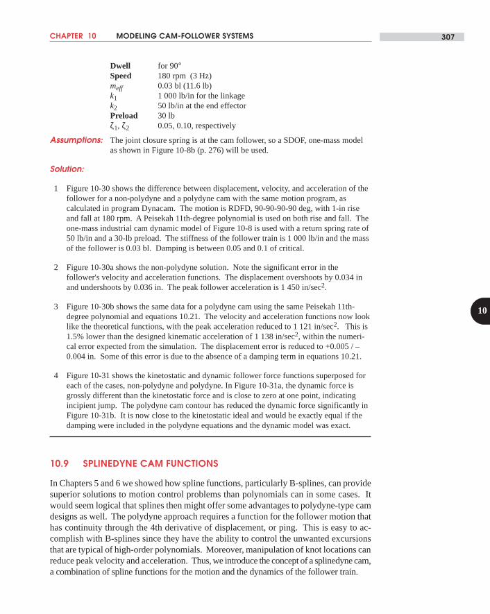
CHAPTER 10 MODELING CAM-FOLLOWER SYSTEMS 307
10
Dwell for 90°Speed 180 rpm (3 Hz)meff 0.03 bl (11.6 lb)k1 1 000 lb/in for the linkagek2 50 lb/in at the end effectorPreload 30 lbζ1, ζ2 0.05, 0.10, respectively
Assumptions: The joint closure spring is at the cam follower, so a SDOF, one-mass modelas shown in Figure 10-8b (p. 276) will be used.
Solution:
1 Figure 10-30 shows the difference between displacement, velocity, and acceleration of thefollower for a non-polydyne and a polydyne cam with the same motion program, ascalculated in program Dynacam. The motion is RDFD, 90-90-90-90 deg, with 1-in riseand fall at 180 rpm. A Peisekah 11th-degree polynomial is used on both rise and fall. Theone-mass industrial cam dynamic model of Figure 10-8 is used with a return spring rate of50 lb/in and a 30-lb preload. The stiffness of the follower train is 1 000 lb/in and the massof the follower is 0.03 bl. Damping is between 0.05 and 0.1 of critical.
2 Figure 10-30a shows the non-polydyne solution. Note the significant error in thefollower's velocity and acceleration functions. The displacement overshoots by 0.034 inand undershoots by 0.036 in. The peak follower acceleration is 1 450 in/sec2.
3 Figure 10-30b shows the same data for a polydyne cam using the same Peisekah 11th-degree polynomial and equations 10.21. The velocity and acceleration functions now looklike the theoretical functions, with the peak acceleration reduced to 1 121 in/sec2. This is1.5% lower than the designed kinematic acceleration of 1 138 in/sec2, within the numeri-cal error expected from the simulation. The displacement error is reduced to +0.005 / –0.004 in. Some of this error is due to the absence of a damping term in equations 10.21.
4 Figure 10-31 shows the kinetostatic and dynamic follower force functions superposed foreach of the cases, non-polydyne and polydyne. In Figure 10-31a, the dynamic force isgrossly different than the kinetostatic force and is close to zero at one point, indicatingincipient jump. The polydyne cam contour has reduced the dynamic force significantly inFigure 10-31b. It is now close to the kinetostatic ideal and would be exactly equal if thedamping were included in the polydyne equations and the dynamic model was exact.
10.9 SPLINEDYNE CAM FUNCTIONS
In Chapters 5 and 6 we showed how spline functions, particularly B-splines, can providesuperior solutions to motion control problems than polynomials can in some cases. Itwould seem logical that splines then might offer some advantages to polydyne-type camdesigns as well. The polydyne approach requires a function for the follower motion thathas continuity through the 4th derivative of displacement, or ping. This is easy to ac-complish with B-splines since they have the ability to control the unwanted excursionsthat are typical of high-order polynomials. Moreover, manipulation of knot locations canreduce peak velocity and acceleration. Thus, we introduce the concept of a splinedyne cam,a combination of spline functions for the motion and the dynamics of the follower train.
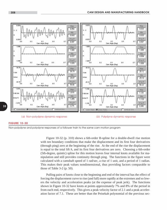
CAM DESIGN AND MANUFACTURING HANDBOOK308
10
FIGURE 10-30
Non-polydyne and polydyne responses of a follower train to the same cam motion program
(a) Non-polydyne dynamic response (b) Polydyne dynamic response
Figure 10-32 (p. 310) shows a 6th-order B-spline for a double-dwell rise motionwith ten boundary conditions that make the displacement and its first four derivatives(through ping) zero at the beginning of the rise. At the end of the rise the displacementis equal to the total lift h, and its first four derivatives are zero. Choosing a 6th-order(5th-degree, quintic) spline for this motion leaves four internal knots available for ma-nipulation and still provides continuity through ping. The functions in the figure werecalculated with a camshaft speed of 1 rad/sec, a rise of 1 unit, and a period of 1 radian.This makes their peak values nondimensional, thus providing factors comparable tothose of Table 3-2 (p. 50).
Pulling pairs of knots close to the beginning and end of the interval has the effect offorcing the displacement curve to rise (and fall) more rapidly at the extremes and so low-ers the velocity and acceleration peaks (at the expense of peak jerk). The functionsshown in Figure 10-32 have knots at points approximately 7% and 8% of the period infrom each end, respectively. This gives a peak velocity factor of 2.1 and a peak acceler-ation factor of 7.1. These are better than the Peisekah polynomial of the previous sec-
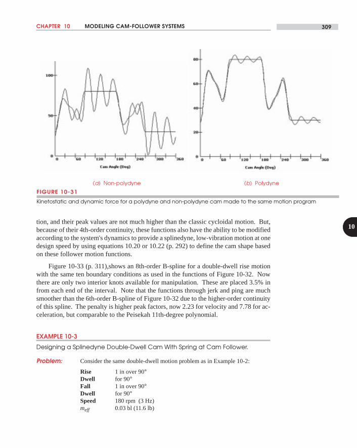
CHAPTER 10 MODELING CAM-FOLLOWER SYSTEMS 309
10tion, and their peak values are not much higher than the classic cycloidal motion. But,because of their 4th-order continuity, these functions also have the ability to be modifiedaccording to the system's dynamics to provide a splinedyne, low-vibration motion at onedesign speed by using equations 10.20 or 10.22 (p. 292) to define the cam shape basedon these follower motion functions.
Figure 10-33 (p. 311),shows an 8th-order B-spline for a double-dwell rise motionwith the same ten boundary conditions as used in the functions of Figure 10-32. Nowthere are only two interior knots available for manipulation. These are placed 3.5% infrom each end of the interval. Note that the functions through jerk and ping are muchsmoother than the 6th-order B-spline of Figure 10-32 due to the higher-order continuityof this spline. The penalty is higher peak factors, now 2.23 for velocity and 7.78 for ac-celeration, but comparable to the Peisekah 11th-degree polynomial.
EXAMPLE 10-3
Designing a Splinedyne Double-Dwell Cam With Spring at Cam Follower.
Problem: Consider the same double-dwell motion problem as in Example 10-2:
Rise 1 in over 90°Dwell for 90°Fall 1 in over 90°Dwell for 90°Speed 180 rpm (3 Hz)meff 0.03 bl (11.6 lb)
FIGURE 10-31
Kinetostatic and dynamic force for a polydyne and non-polydyne cam made to the same motion program
(a) Non-polydyne (b) Polydyne
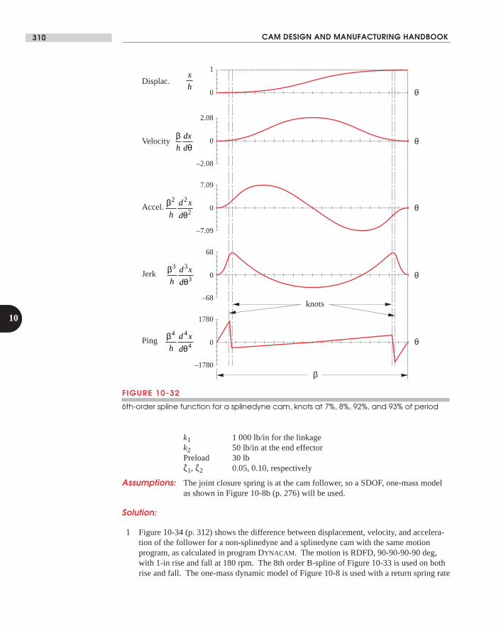
CAM DESIGN AND MANUFACTURING HANDBOOK310
10
k1 1 000 lb/in for the linkagek2 50 lb/in at the end effectorPreload 30 lbζ1, ζ2 0.05, 0.10, respectively
Assumptions: The joint closure spring is at the cam follower, so a SDOF, one-mass modelas shown in Figure 10-8b (p. 276) will be used.
Solution:
1 Figure 10-34 (p. 312) shows the difference between displacement, velocity, and accelera-tion of the follower for a non-splinedyne and a splinedyne cam with the same motionprogram, as calculated in program DYNACAM. The motion is RDFD, 90-90-90-90 deg,with 1-in rise and fall at 180 rpm. The 8th order B-spline of Figure 10-33 is used on bothrise and fall. The one-mass dynamic model of Figure 10-8 is used with a return spring rate
0
2.08
0
0
0
–2.08
7.09
–7.09
68
–68
1780
–1780
0
1
β
Displac.
Velocity
Accel.
Jerk
Ping
βθ
2 2
2h
d x
d
x
h
βθ
3 3
3h
d x
d
βθh
dx
d
βθ
4 4
4h
d x
d
θ
θ
θ
θ
θ
knots
FIGURE 10-32
6th-order spline function for a splinedyne cam, knots at 7%, 8%, 92%, and 93% of period
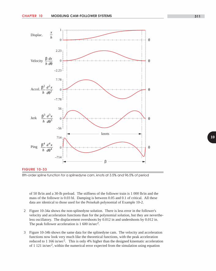
CHAPTER 10 MODELING CAM-FOLLOWER SYSTEMS 311
10
of 50 lb/in and a 30-lb preload. The stiffness of the follower train is 1 000 lb/in and themass of the follower is 0.03 bl. Damping is between 0.05 and 0.1 of critical. All thesedata are identical to those used for the Peisekah polynomial of Example 10-2.
2 Figure 10-34a shows the non-splinedyne solution. There is less error in the follower'svelocity and acceleration functions than for the polynomial solution, but they are neverthe-less oscillatory. The displacement overshoots by 0.012 in and undershoots by 0.012 in.The peak follower acceleration is 1 600 in/sec2.
3 Figure 10-34b shows the same data for the splinedyne cam. The velocity and accelerationfunctions now look very much like the theoretical functions, with the peak accelerationreduced to 1 166 in/sec2. This is only 4% higher than the designed kinematic accelerationof 1 121 in/sec2, within the numerical error expected from the simulation using equation
0
2.23
0
0
0
–2.23
7.78
–7.78
56
–56
714
–714
0
1
β
Displac.
Velocity
Accel.
Jerk
Ping
βθ
2 2
2h
d x
d
x
h
βθ
3 3
3h
d x
d
βθh
dx
d
βθ
4 4
4h
d x
d
θ
θ
θ
θ
θ
knots
FIGURE 10-33
8th-order spline function for a splinedyne cam, knots at 3.5% and 96.5% of period
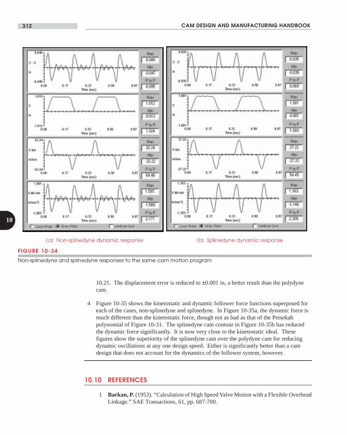
CAM DESIGN AND MANUFACTURING HANDBOOK312
10
FIGURE 10-34
Non-splinedyne and splinedyne responses to the same cam motion program
(a) Non-splnedyne dynamic response (b) Splinedyne dynamic response
10.21. The displacement error is reduced to ±0.001 in, a better result than the polydynecam.
4 Figure 10-35 shows the kinetostatic and dynamic follower force functions superposed foreach of the cases, non-splinedyne and splinedyne. In Figure 10-35a, the dynamic force ismuch different than the kinetostatic force, though not as bad as that of the Peisekahpolynomial of Figure 10-31. The splinedyne cam contour in Figure 10-35b has reducedthe dynamic force significantly. It is now very close to the kinetostatic ideal. Thesefigures show the superiority of the splinedyne cam over the polydyne cam for reducingdynamic oscillations at any one design speed. Either is significantly better than a camdesign that does not account for the dynamics of the follower system, however.
10.10 REFERENCES
1 Barkan, P. (1953). “Calculation of High Speed Valve Motion with a Flexible OverheadLinkage.” SAE Transactions, 61, pp. 687-700.
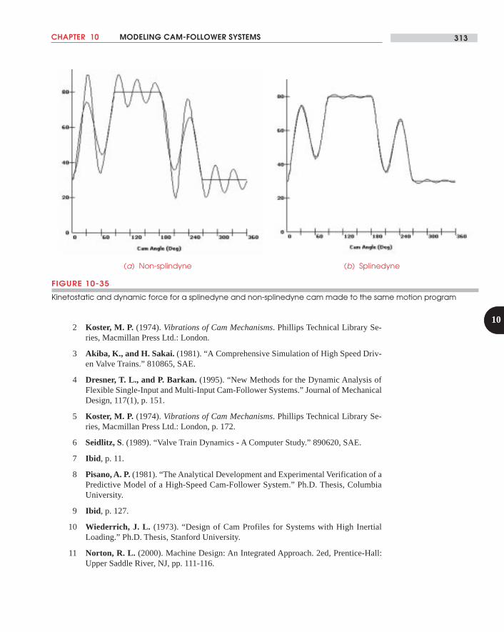
CHAPTER 10 MODELING CAM-FOLLOWER SYSTEMS 313
102 Koster, M. P. (1974). Vibrations of Cam Mechanisms. Phillips Technical Library Se-
ries, Macmillan Press Ltd.: London.
3 Akiba, K., and H. Sakai. (1981). “A Comprehensive Simulation of High Speed Driv-en Valve Trains.” 810865, SAE.
4 Dresner, T. L., and P. Barkan. (1995). “New Methods for the Dynamic Analysis ofFlexible Single-Input and Multi-Input Cam-Follower Systems.” Journal of MechanicalDesign, 117(1), p. 151.
5 Koster, M. P. (1974). Vibrations of Cam Mechanisms. Phillips Technical Library Se-ries, Macmillan Press Ltd.: London, p. 172.
6 Seidlitz, S. (1989). “Valve Train Dynamics - A Computer Study.” 890620, SAE.
7 Ibid , p. 11.
8 Pisano, A. P. (1981). “The Analytical Development and Experimental Verification of aPredictive Model of a High-Speed Cam-Follower System.” Ph.D. Thesis, ColumbiaUniversity.
9 Ibid , p. 127.
10 Wiederrich, J. L. (1973). “Design of Cam Profiles for Systems with High InertialLoading.” Ph.D. Thesis, Stanford University.
11 Norton, R. L. (2000). Machine Design: An Integrated Approach. 2ed, Prentice-Hall:Upper Saddle River, NJ, pp. 111-116.
FIGURE 10-35
Kinetostatic and dynamic force for a splinedyne and non-splinedyne cam made to the same motion program
(a) Non-splindyne (b) Splinedyne

CAM DESIGN AND MANUFACTURING HANDBOOK314
10
12 Thoren, T. R., et al. (1952). “Cam Design as Related to Valve Train Dynamics.” SAEQuarterly Transactions, 6(1), pp. 1-14.
13 Dudley, W. M. (1948). “New Methods in Valve Cam Design.” SAE Quarterly Transac-tions, 2(1), pp. 19-33.
14 Stoddart, D. A. (1953). “Polydyne Cam Design-I.” Machine Design, January, 1953,pp. 121-135.
15 Stoddart, D. A. (1953). “Polydyne Cam Design-II.” Machine Design, February, 1953,pp. 146-154.
16 Stoddart, D. A. (1953). “Polydyne Cam Design-III.” Machine Design, March, 1953,pp. 149-164.
17 Norton, R. L., et al. (1999). “Effect of Valve-Cam Ramps on Valve Train Dynamics.”SAE 1999-01-0801.
18 Mosier, R. G. (2000). “Modern Cam Design.” Int. J. Vehicle Design, 23(1/2), pp. 38-55.
19 Peisekah, E. E. (1966). “Improving the Polydyne Cam Design Method.” Russian En-gineering Journal, XLVI(12), pp. 25-27.
20 Fawcett, G. F., and J. N. Fawcett, eds. (1978). “Comparison of Polydyne and Non-Polydyne Cams.” Cams and Cam Mechanisms, Jones, J. R., ed., Institution of Mechan-ical Engineers: London.
21 Press, W. H., et al. (1986). Numerical Recipes: The Art of Scientific Computing. Cam-bridge University Press: Cambridge, pp. 547-577.