Modeling and Prediction of the 2019 Coronavirus …...Modeling and Prediction of the 2019...

Modeling and Prediction of the 2019 Coronavirus Disease Spreading in ChinaIncorporating Human Migration Data

Choujun Zhana, Chi K. Tseb,∗, Yuxia Fuc, Zhikang Laic, Haijun Zhangd

aSchool of Computing, South China Normal University, Guangzhou, ChinabDepartment of Electrical Engineering, City University of Hong Kong, Hong Kong.

cSchool of Computer Science and Engineering, Nanfang College of Sun Yat-Sen University, ChinadShenzhen Graduate School, Harbin Institute of Technology, Shenzhen, China

Abstract

This study integrates the daily intercity migration data with the classic Susceptible-Exposed-Infected-Removed (SEIR)model to construct a new model suitable for describing the dynamics of epidemic spreading of Coronavirus Disease2019 (COVID-19) in China. Daily intercity migration data for 367 cities in China are collected from Baidu Migra-tion, a mobile-app based human migration tracking data system. Historical data of infected, recovered and death casesfrom official source are used for model fitting. The set of model parameters obtained from best data fitting using aconstrained nonlinear optimization procedure is used for estimation of the dynamics of epidemic spreading in thecoming weeks. Our results show that the number of infections in most cities in China will peak between mid Februaryto early March 2020, with about 0.8%, less than 0.1% and less than 0.01% of the population eventually infected inWuhan, Hubei Province and the rest of China, respectively.

Keywords: Epidemic spreading, COVID-19, new coronavirus, human migration, intercity travel.

1. Introduction

The Coronavirus Disease 2019 (COVID-19) (known earlier as New Coronavirus Infected Pneumonia) began tospread since December 2019 from Wuhan, which has been widely regarded as the epicenter of the epidemic, to almostall provinces throughout China and 28 other countries. Human-to-human transmission had been found to occur insome early Wuhan cases in mid December [1], and the high volume and frequency of movement of people from Wuhanto other cities and between cities is thus an obvious cause for the wide and rapid spread of the disease throughout thecountry. The Susceptible-Exposed-Infected-Removed (SEIR) model has traditionally been used to study epidemicspreading with various forms of networks of transmission which define the contact topology [2], such as scalefreenetworks [3, 4, 5], small-world networks [6, 7], Oregon graph [8, 9], and adaptive networks [10]. Moreover, in moststudies, the contact process assumes that the contagion expands at a certain rate from an infected individual to his/herneighbor, and that the spreading process takes place in a single population (network). The COVID-19 outbreak,however, began to occur and escalate in a special holiday period in China (about 20 days surrounding the Lunar NewYear), during which a huge volume of intercity travel took place, resulting in outbreaks in multiple regions connectedby an active transportation network. Thus, in order to understand the COVID-19 spreading process in China, itis essential to examine the human migration dynamics, especially between the epicenter Wuhan and other Chinesecities. A recent study has also revealed the risk of transmission of the virus from Wuhan to other cities [11].

In this paper, we utilize the human migration data collected from Baidu Migration [12], which provides historicalindicative daily volume of travellers to/from and between 367 cities in China. To demonstrate the impact of intercitytraffic on the COVID-19 epidemic spreading, we plot in Figure 1 the number of infected individuals in differentcities versus the inflow traffic volume from Wuhan, which clearly shows that for cities farther away from Wuhan,

∗Corresponding authorEmail address: [email protected] (Chi K. Tse)

Preprint submitted to medrxiv.org February 19, 2020

. CC-BY-NC 4.0 International licenseIt is made available under a is the author/funder, who has granted medRxiv a license to display the preprint in perpetuity.

(which was not peer-reviewed) The copyright holder for this preprint .https://doi.org/10.1101/2020.02.18.20024570doi: medRxiv preprint

https://doi.org/10.1101/2020.02.18.20024570

http://creativecommons.org/licenses/by-nc/4.0/

102

103

104

105

106

107

0

500

1000

1500

2000

2500

3000

Figure 1: Number of infected individuals in various cities on 13/Feb/2020 versus the city’s inflow traffic from Wuhan. Inflow traffic of each cityfrom Wuhan is quantified by migration strength from Wuhan extracted from Baidu Migration data.

the number of infected individuals almost increases linearly with the inflow traffic from Wuhan. In view of theimportance of human migration dynamics to the disease spreading process, we combine, in this study, intercity traveldata collected from Baidu Migration [12] with the traditional SEIR model [2] to build a new dynamic model for thespreading of COVID-19 in China. Using official historical data of infected, recovered and death cases in 367 cities,we perform fitting of the data to estimate the best set of model parameters, which are then used to estimate the numberof individuals exposed to the virus in each city and to predict the extent of spreading in the coming months. Our studyshows that the number of infected cases in various Chinese cities will peak between mid February to early March2020, with about 0.8%, less than 0.1% and less than 0.01% of the population eventually infected in Wuhan, HubeiProvince, and the rest of China, respectively.

In the remainder of the paper, we first introduce the official daily infection data and the intercity migration dataused in this study. The SEIR model is modified to incorporate the human migration dynamics, giving a realisticmodel suitable for studying the COVID-19 epidemic spreading dynamics. Historical data of infected, recovered anddeath cases from official source and data of daily intercity traffic (number of travellers between cities) extracted fromBaidu Migration are used to generate the model parameters, which then enable estimation of the propagation of theepidemic in the coming months. We will conclude with a brief discussion of our estimation of the propagation and thereasonableness of our estimation in view of the measures taken by the Chinese authorities in controlling the spreadingof this new disease.

2. Data

2.1. Official Data of COVID-19 Cases

The availability of official data of infected cases in China varies from city to city. Wuhan, being the epicenter, hasthe first confirmed case of COVID-19 infection on December 8, 2019 [1]. Most other cities in China began to reportcases of COVID-19 infections around mid January 2020. Our data of daily infected and recovered cases, and deathtolls, are based on the official data released by the National Health Commission of China, and the daily data used inour study are from January 24, 2020, to February 16, 2020, including the daily total number of confirmed cases ineach city, daily total cumulative number of confirmed cases in each city, daily cumulative number of recovered casesin each city, and daily cumulative death toll in each city. It should be emphasized that the official data may not bethe actual (true) data. Although the earliest confirmed case appeared on December 8, 2019, subsequent missing caseswere expected to be significant in Hubei Province in the early stage of the epidemic outbreak. Systematic updates of

2



https://doi.org/10.1101/2020.02.18.20024570


08Dec19 19Dec19 31Dec19 12Jan20 23Jan20 04Feb20 16Feb20

0

1

2

3

410

4

(a) Wuhan

20Jan20 24Jan20 29Jan20 02Feb20 07Feb20 11Feb20 16Feb20

0

100

200

300

400

(b) Beijing


0

100

200

300

400

500

600

(c) Shanghai


0

100

200

300

400

500

(d) Shenzhen


0

100

200

300

400

(e) Guangzhou


0

50

100

150

(f) Tinajin

Figure 2: Daily data of COVID-19 infections in six Chinese cities from December 8, 2019 to February 13, 2020. (a) Wuhan (available fromDecember 8, 2019); (b) Beijing (available from January 20, 2020); (c) Chongqing (available from January 20, 2020); (d) Shenzhen (available fromJanuary 19, 2020); (e) Guangzhou (available from January 21, 2020); (d) Tianjin (available from January 21, 2020).

infection data in other cities began after January 17, 2020. Figure 2 shows the number of confirmed infected cases,recovered cases and death tolls of six major Chinese cities.

2.2. Intercity Travel Data

As human-to-human transmission has been confirmed to occur in the spreading of COVID-19, gatherings ofpeople and intercity travel of infected and exposed individuals within China have been the main drives that escalatethe spreading of the virus. The period (around 20 days) surrounding the Lunar New Year (mid January to earlyFebruary in 2020) is the most important holiday period in China. Migrant workers and students travel from majorcities to country towns for family reunions, and return to the cities at the end of the holiday period. Holiday goersalso travel to and from tourist cities. China’s Ministry of Transport estimates around 3 billion trips to be taken duringthis period. Wuhan, being a major transport hub and having a large number of higher education institutions as well asmanufacturing plants, is among the cities with the largest outflow and inflow traffic before and after the Chinese NewYear festival. Our study aims to incorporate these important human migration dynamics in the construction of thespreading model. We collect daily intercity travel data in China from Baidu Migration, which is a mobile-app basedbig data system recording movements of mobile phone users. Specifically, we have collected Baidu Migration datafor 367 cities (or administrative regions) in China over the period of January 1, 2020, to February 13, 2020. The dataprovide the migration strengths of cities which are indicative measures of the human traffic volume moving in and outof individual cities and administrative regions, as depicted by the inflow and outflow networks shown in Figure 3(a).

3



https://doi.org/10.1101/2020.02.18.20024570


(a)

(b)

Figure 3: (a) Illustration of travel network of major cities in China with arrows indicating direction of travel and darkness of lines indicating mi-gration strengths (relative traffic volumes); (b) total inflow/outflow of travellers to/from Wuhan from/to other Chinese cities using Baidu Migrationdata. Inflow and outflow data of each city with individual cities are also collected to form mi j.

Based on the collected data, we construct the migration matrix, which is given as

M(t) =

m11(t) m12(t) · · · m1K(t)m21(t) m22(t) · · · m2K(t)...

.... . .

...mN1(t) mN2(t) · · · mKK(t)

, (1)

4



https://doi.org/10.1101/2020.02.18.20024570


50 100 150 200 250 300 350

Index of cities

50

100

150

200

250

300

350

Index o

f citie

s

2

4

6

8

10

12

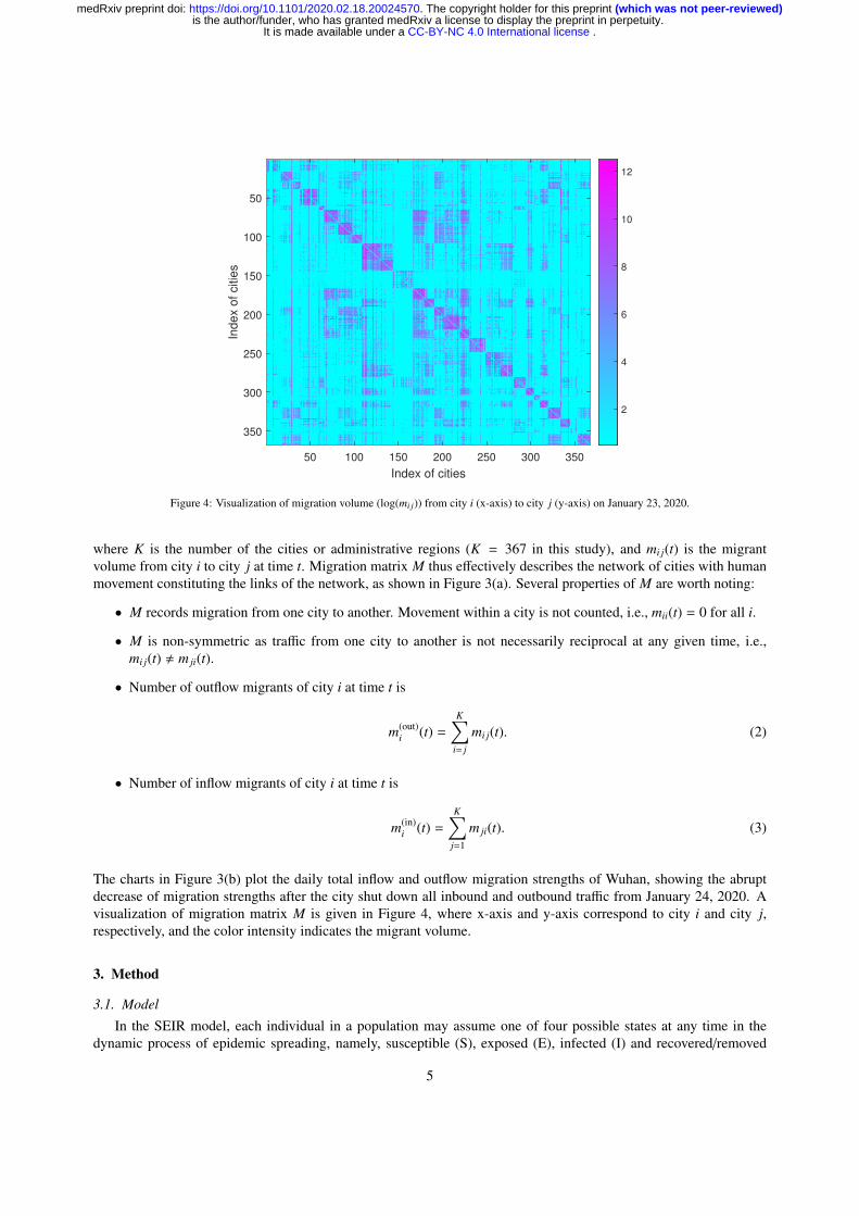
Figure 4: Visualization of migration volume (log(mi j)) from city i (x-axis) to city j (y-axis) on January 23, 2020.

where K is the number of the cities or administrative regions (K = 367 in this study), and mi j(t) is the migrantvolume from city i to city j at time t. Migration matrix M thus effectively describes the network of cities with humanmovement constituting the links of the network, as shown in Figure 3(a). Several properties of M are worth noting:

• M records migration from one city to another. Movement within a city is not counted, i.e., mii(t) = 0 for all i.

• M is non-symmetric as traffic from one city to another is not necessarily reciprocal at any given time, i.e.,mi j(t) , m ji(t).

• Number of outflow migrants of city i at time t is

m(out)i (t) =

K∑i= j

mi j(t). (2)

• Number of inflow migrants of city i at time t is

m(in)i (t) =

K∑j=1

m ji(t). (3)

The charts in Figure 3(b) plot the daily total inflow and outflow migration strengths of Wuhan, showing the abruptdecrease of migration strengths after the city shut down all inbound and outbound traffic from January 24, 2020. Avisualization of migration matrix M is given in Figure 4, where x-axis and y-axis correspond to city i and city j,respectively, and the color intensity indicates the migrant volume.

3. Method

3.1. Model

In the SEIR model, each individual in a population may assume one of four possible states at any time in thedynamic process of epidemic spreading, namely, susceptible (S), exposed (E), infected (I) and recovered/removed

5



https://doi.org/10.1101/2020.02.18.20024570


(R). The dynamics of the epidemic can be described by the following set of equations: S (t) = −βS (t)I(t), E(t) =

βS (t)I(t) − kE(t), I(t) = κE(t) − γI(t), and R(t) = γI(t), where S (t), E(t), I(t) and R(t) are, respectively, the number ofpeople susceptible to the disease, exposed (being able to infect others but having no symptoms), infected (diagnosedas confirmed cases), and recovered (including death cases); β is the exposition rate (infection rate of susceptibleindividuals); κ is the infection rate of exposed individuals; and γ is the recovery rate. For simplicity, recoveredindividuals include patients recovered from the disease and death tolls. In discrete form, the SEIR model can berepresented by

∆S (t) = −βS (t − 1)I(t − 1),∆E(t) = βS (t − 1)I(t − 1) − κE(t − 1),∆I(t) = κE(t − 1) − γI(t − 1),∆R(t) = γI(t − 1)

(4)

where ∆S (t) = S (t)− S (t− 1), ∆E(t) = E(t)− E(t− 1), ∆I(t) = I(t)− I(t− 1), and ∆R(t) = R(t)−R(t− 1), with t beinga daily count. As the incubation period for COVID-19 can be up to 14 days, the number of exposed individuals (whoshow no symptom but are able to infect others) plays a crucial role in the spreading of the disease. The state E, whichis not available from the official data, is thus an important state in our model. Furthermore, combining death toll withthe recovered number as state R will simplify the computation without affecting the accuracy of our data fitting andsubsequent estimation.

Suppose, for city i, the four states are S i(t), Ei(t), Ii(t) and Ri(t), at time t. Here, we also define a total susceptiblepopulation, N s

i , which is the eventual number of infected individuals in city i. Moreover, if city i has a population ofPi and the eventual percentage of infection is δi, then N s

i = δiPi. Thus, we have

N si (t) = S i(t) + Ei(t) + Ii(t) + Ri(t). (5)

The classic SEIR model would give ∆Ii as the difference between the number of exposed individuals who becomeinfected and the number of removed individuals. However, the onset of the COVID-19 epidemic has occurred ina special period of time in China, during which a huge migration traffic is being carried among cities, leading to ahighly rapid transmission of the disease throughout the country. In view of this special migration factor, the SEIRmodel should incorporate the human migration dynamics in order to capture the essential features of the dynamics ofthe spreading. In particular, for city i, in addition to the abovementioned classic interpretation, the daily increase in thenumber of infected cases should also include the inflow of infected individuals from other cities, less the outflow ofremoved cases from city i. In reality, inflow and outflow of exposed individuals to and from the city are also importantand to be estimated in the model. Thus, if mi j(t) people move from city i to city j on day t, and the population of cityi is Pi(t), then the number of infected individuals moving from city i to city j is

∆Iini j (t) =

Ii(t)mi j(t)Pi

. (6)

Also, the number of migrants leaving from city j is∑N

i=1 m ji, and the number of infected cases that have migrated outof city j is

∆Ioutj (t) =

I j(t)∑N

i=1 m ji(t)P j

, (7)

where P j(t) is the population of city j on day t. Thus, the increase in infected cases on day t in city j is given by

∆I j(t) = κ j(t)Ei(t) − γ(t)I j(t) +

N∑i=1

∆Iini j (t) − ∆Iout

j (t)

= κ j(t)Ei(t) − γ j(t)I j(t) +

N∑i=1

ÅIi(t)mi j(t)

Pi(t)

ã−

I j(t)∑N

i=1 m ji(t)P j(t)

,

(8)

where ∆I j(t) = I j(t+1)− I j(t) and κ j(t) is the infection rate in city j on day t, i.e., the rate at which exposed individualsbecome infected. Moreover, infected individuals, once confirmed, would unlikely be able to migrate to another city.

6



https://doi.org/10.1101/2020.02.18.20024570


We thus implement this condition by writing (8) as

∆I j(t) = κ j(t)Ei(t) − γ j(t)I j(t) + kI

(N∑

i=1

ÅIi(t)mi j(t)

Pi(t)

ã−

I j(t)∑N

i=1 m ji(t)P j(t)

), (9)

where 0 < kI � 1 is a constant representing the possibility of an infected individual moving from one city to another.Likewise, incorporating the migrant dynamics, the increase in exposed individuals on day t in city j is

∆E j(t) =β j(t)N s

j (t)I j(t)S j(t) +

α j(t)N s

j (t)E j(t)S j(t) − κ j(t)Ei(t) +

N∑i=1

ÅEi(t)mi j(t)

Pi(t)

ã−

E j(t)∑N

i=1 m ji(t)P j(t)

, (10)

where ∆E j(t) = E j(t + 1)−E j(t), β j is the infection rate of susceptible individuals in city j, and α j is the infection rateof exposed individuals in city j. In a likewise fashion, we have

∆S j(t) = −β j(t)N s

j (t)I j(t)S j(t) −

α j(t)N s

j (t)E j(t)S j(t) +

N∑i=1

ÅS i(t)mi j(t)

Pi(t)

ã−

S j(t)∑N

i=1 m ji(t)P j(t)

, (11)

where ∆S j(t) = S j(t + 1) − S j(t). Finally, we have

∆R j(t) = γ j(t)I j(t), (12)

where ∆R j(t) = R j(t + 1) − R j(t). In the above derivation, we should note that

• the recovered individuals are assumed to stay in city j;

• the recovery rates in different cities are assumed to be different due to varied quality of treatments and avail-ability of medical facilities;

• the recovery rates increase as time goes, as treatment methods are expected to improve gradually (i.e., takingγ j(t) as a monotonically increasing function);

• the evetual recovery rates in all cities will converge to the same constant Γ ≈ 1.

In addition, due to intercity migration, the population of city j on day t would increase or decrease according to

∆P j(t) =

N∑i=1

ÅPi(t)mi j(t)

Pi(t)

ã−

P j(t)∑N

i=1 m ji(t)P j(t)

=

N∑i=1

mi j(t) −N∑

i=1

m ji(t), (13)

where ∆P j(t) = P j(t + 1) − P j(t). Thus, the total susceptible population should be

∆N sj (t) = kI

(N∑

i=1

ÅIi(t)mi j(t)

Pi(t)

ã−

I j(t) ∗∑N

i=1 m ji(t)P j(t)

)+

N∑i=1

ÅEi(t)mi j(t)

Pi(t)

ã−

E j(t) ∗∑N

i=1 m ji(t)P j(t)

+

N∑i=1

ÅS i(t)mi j(t)

Pi(t)

ã−

S j(t)∑N

i=1 m ji(t)P j(t)

.

(14)

where ∆N sj (t) = N s

j (t + 1) − N sj (t).

7



https://doi.org/10.1101/2020.02.18.20024570


In summary, our modified SEIR model with consideration of human migration dynamics, for city j, is given by

∆I j(t) = κ j(t)Ei(t) − γ j(t)I j(t) + kI

(N∑

i=1

ÅIi(t)mi j(t)

Pi(t)

ã−

I j(t) ∗∑N

i=1 m ji(t)P j(t)

),

∆E j(t) =β j(t)N s

j (t)I j(t)S j(t) +

α j(t)N s

j (t)E j(t)S j(t) − κ j(t)Ei(t) +

N∑i=1

ÅEi(t)mi j(t)

Pi(t)

ã−

E j(t) ∗∑N

i=1 m ji(t)P j(t)

,

∆S j(t) = −β j(t)N s

j (t)I j(t)S j(t) −

α j(t)N s

j (t)E j(t)S j(t) +

N∑i=1

ÅS i(t)mi j(t)

Pi(t)

ã−

S j(t)∑N

i=1 m ji(t)P j(t)

,

∆R j(t) = γ j(t)I j(t),

∆P j(t) =

N∑i=1

mi j(t) −N∑

i=1

m ji(t),

∆N sj (t) = kI

(N∑

i=1

ÅIi(t)mi j(t)

Pi(t)

ã−

I j(t) ∗∑N

i=1 m ji(t)P j(t)

)+

N∑i=1

ÅEi(t)mi j(t)

Pi(t)

ã−

E j(t) ∗∑N

i=1 m ji(t)P j(t)

+

N∑i=1

ÅS i(t)mi j(t)

Pi(t)

ã−

S j(t)∑N

i=1 m ji(t)P j(t)

.

(15)

where subscript j denotes the city itself, and subscript i denotes another city from/to which people migrate on dayt. Letting X j(t) be the extended state vector, i.e., X j(t) = [S j(t) E j(t) I j(t) R j(t) P j(t) N s

j (t)]T , we write the above

difference equation as∆X j(t) = f (X j, Xi, µi) (16)

where f (x) is the right side of (15), and µ j is the set of parameters including α j, β j, γ j, κ j and δ j. For computationalconvenience, we write (15) as

X j(t + 1) = X j(t) + f (X j, Xi, µi) (17)

In performing the data fitting, we assume α j(t), β j(t), γ j(t), κ j(t), and δ j are constants throughout the period ofspreading, and the spreading begins at t0, at which N s

j (t0) = δ jP j(t0).

3.2. Parameter Identification

The model represented by (17) describes the dynamics of the epidemic propagation with consideration of humanmigration dynamics. The parameters in model (17) are unknown and to be estimated from historical data. We solvethis parameter identification problem via constrained nonlinear programming (CNLP), with the objective of findingan estimated growth trajectory that fits the data. An estimated number of infected cases of each city can be generatedfrom (15) with unknown set θ j, i.e.,

θ j = {α j, β j, γ j, κ j, δ j, I j,0} (18)

where I j,0 = I j(t0) is the initial number of infections in city j, and {α j, β j, γ j, κ j, δ j} are parameters that determine therates of spreading and recovery in city j. Then, the unknown set is Θ = {θ1, θ2, · · · , θK} essentially has 5K unknowns,where K is the number of cities, thus requiring an enormous effort of computation. Here, to gain computationalefficiency, we assume that

• all cities share one parameter set θ = {α, β, κ, γ};

• the numbers of initial infected and exposed individuals in city i are λI Ii(t0) and λE Ii(t0), respectively, where λI

and λE are constant;

• each city has an independent δi.

8



https://doi.org/10.1101/2020.02.18.20024570


Then, the size of the unknown set becomes computationally manageable, i.e.,

Θ = {α, β, κ, γ, δi, λI , λE}.

Finally, the parameter estimation problem can be formulated as the following constrained nonlinear optimizationproblem:

P0: minΘ

N∑j=0

∥∥∥w j(I(t j) − I(t j))∥∥∥

l

s.t.ß

(i) x(t + 1) = x(t) + F(x(t)),(ii) ΘU ≥ Θ ≥ ΘL,

(19)

where F(·) represents model (15) and x(t) = [I(t), R(t), E(t), S (t), P(t),N s(t)] is the set of estimated variables, withunknown set Θ, which is bounded between ΘL and ΘU . In this work, an inverse approach is taken to find the unknownparameters and states by solving (19).

The Root Mean Square Percentage Error (RMSPE) is adopted as the criterion, i.e., fitting error, to measure thedifference between the number of infected individuals generated by the model and the official daily infection data.

RMSPE =

Ã1K

∑i=1

∑j=1

ÇIi(t j) − Ii(t j)

Ii(t j)

å2

× 100%, (20)

where K is the number of cities to be evaluated.

4. Results and Discussions

We perform data fitting of the model, described by (17), using historical daily infection data provided by theNational Health Commission of China, from January 24, 2020 to February 13, 2020. Our approach, as described inthe previous section, is to apply constrained nonlinear programming to find the best set of estimates for the unknownparameters and states. Data fitting for all 367 cities are performed. Values are updated iteratively in the optimizationprocess. Moreover, since all parameters, like infection rates, are to be generated by fitting data with the model, theintegrity of the data becomes crucial. As the official Wuhan data are expected to deviate from the true values quitesignificantly during the early outbreak stage due to uncertainty in diagnosis and other issues related to reporting of theepidemic by the local government, we have allowed the fitting errors for Wuhan to expand over a reasonable range,while the fitting errors for most other cities remain small. In addition, as the epidemic propagates in time, effectivecontrol measures and improved public education would reduce the infection rates for the susceptible and exposedindividuals, making these parameters time varying in reality. Nonetheless, our fitting assumes these parameters beingconstant during the short fitting period for computational simplicity.

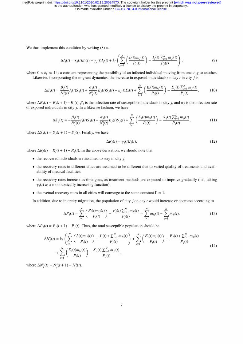
The propagation profiles, in terms of the number of infected individuals and estimated number of exposed individ-uals, for all 367 cities are estimated. As limited by space, we only show in Figure 5 the results for 20 selected cities.This model can also provide projections of the number of infected and exposed individuals in the next 200 days, asshown in Figure 6, which clearly show that the daily infection would reach a peak sooner or later. By running the iden-tification algorithm, we identify the optimal parameter set as α = 0.5869, β = 0.8949, κ = 0.1008, and γ = 0.0602.From the estimated propagation profiles of the COVID-19 epidemic for all 367 cities, we have the following findings:

• For most cities in China, the infection numbers will peak between mid February to early March 2020, as shownin Figure 7(a).

• The peak number of infected individuals will be between 1,000 to 5,000 for cities in Hubei, and that outsideHubei will be below 500, as shown in Figure 7(b).

• At the end, about 0.8%, less than 0.1% and less than 0.01% of the population will get infected in Wuhan, HubeiProvince and the rest of China, respectively, as graphically presented in Figure 7(c).

9



https://doi.org/10.1101/2020.02.18.20024570



100

200

300

Number of infections (official)

Number of infections (estimated)


50

100

150

200

Number of exposed (estimated)

(a) Beijing


100

200

300




50

100

150

200

250


(b) Guangzhou


50

100

150




20

40

60

80

100 Number of exposed (estimated)

(c) Haerbin


1000

2000

3000




500

1000

1500

2000


(d) Huanggang


200

400

600

800

1000




200

400

600


(e) Jingmen


500

1000

1500




200

400

600

800

1000


(f) Jingzhou


10

20

30

40

50




10

20

30Number of exposed (estimated)

(g) Lianyungang


20

40

60




10

20

30

40


(h) Qingdao


100

200

300




50

100

150

200

250


(i) Shanghai


100

200

300




50

100

150

200

250


(j) Shenzhen


100

200

300

400

500




100

200

300


(k) Chongqing


20

40

60

80

100




20

40


(l) Suzhou


10

20

30

40

50




10

20

30

40


(m) Tangshan


20

40

60

80

100




20

40

60

80


(n) Tianjin


100

200

300

400

500




100

200


(o) Tianmen


20

40

60

80

100




20

40

60

80


(p) Xian


20

40

60




10

20

30

40


(q) Hong Kong


1000

2000

3000




500

1000

1500

2000

2500


(r) Xiaogan


200

400

600

800

1000




200

400


(s) Yichang


20

40

60




10

20

30

40


(t) Zhongshan

Figure 5: Official number of infected individuals and estimated number of infected individuals in 20 selected cities in China (upper), and estimatednumber of exposed individuals (lower).

Opinions diverge in the social media on the estimated extent of the outbreak of the new coronavirus disease(COVID-19). While there are pure speculations, there are also predictions based on rigorous study of the spreadingdynamics. Different models used for prediction and different assumptions made regarding the transmission process

10



https://doi.org/10.1101/2020.02.18.20024570


24Jan20 01Mar20 07Apr20 14May20 20Jun20 27Jul20 02Sep200

100

200

300




50

100

150

200


(a) Beijing


100

200

300




50

100

150

200

250


(b) Guangzhou


50

100

150Number of infections (official)



20

40

60

80

100 Number of exposed (estimated)

(c) Haerbin


1000

2000

3000




500

1000

1500

2000


(d) Huangang


200

400

600

800

1000




200

400

600


(e) Jingmen


500

1000

1500




200

400

600

800


(f) Jingzhou


10

20

30

40

50




10

20


(g) Lianyungang


20

40

60




10

20

30

40


(h) Qingdao


100

200

300




50

100

150

200

250


(i) Shanghai


100

200




50

100

150

200

250


(j) Shenzhen


200

400

600




100

200

300


(k) Chongqing


20

40

60

80

100




20

40


(l) Suzhou


10

20

30

40

50




10

20

30

40


(m) Tangshan


20

40

60

80

100 Number of infections (official)



20

40

60

80


(n) Tianjin


100

200

300

400

500




100

200


(o) Tianmen


20

40

60

80




20

40

60

80


(p) Xian


20

40

60




10

20

30

40


(q) Hong Kong


1000

2000

3000




500

1000

1500

2000

2500


(r) Xiaogan


200

400

600

800

1000




200

400

600

800


(s) Yichang


20

40

60




10

20

30

40


(t) Zhongshan

Figure 6: Prediction of the number of infected (upper) and exposed individuals (lower) in 20 selected cites in China for the next 200 days Chongqingfor the next 200 days.

would lead to different results and quite diverged conclusions. For instance, an AI-powered simulation run hadforecasted 2.5 billion people to be infected in 45 days [13]. Academics in Hong Kong expected 1.4 million eventuallyinfected in the city of 7.5 million people. Our results, however, do not seem to agree with such forecasts. In fact, our

11



https://doi.org/10.1101/2020.02.18.20024570


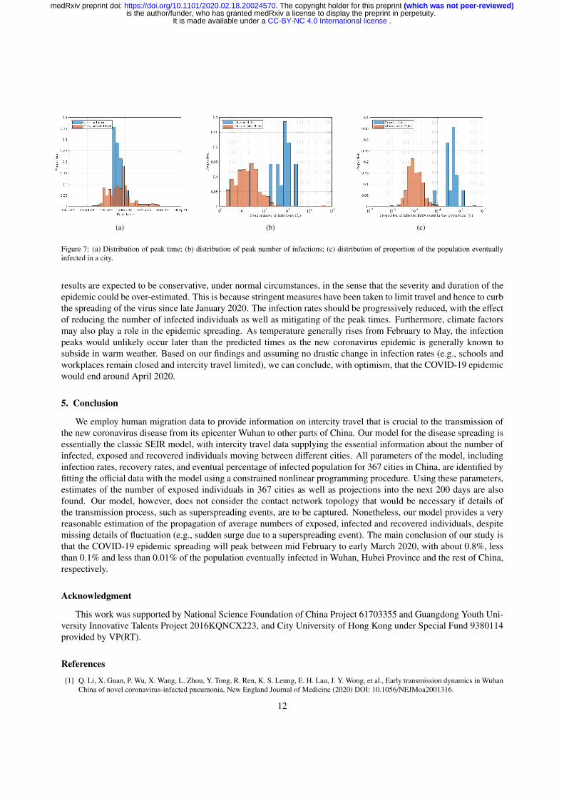
(a) (b) (c)

Figure 7: (a) Distribution of peak time; (b) distribution of peak number of infections; (c) distribution of proportion of the population eventuallyinfected in a city.

results are expected to be conservative, under normal circumstances, in the sense that the severity and duration of theepidemic could be over-estimated. This is because stringent measures have been taken to limit travel and hence to curbthe spreading of the virus since late January 2020. The infection rates should be progressively reduced, with the effectof reducing the number of infected individuals as well as mitigating of the peak times. Furthermore, climate factorsmay also play a role in the epidemic spreading. As temperature generally rises from February to May, the infectionpeaks would unlikely occur later than the predicted times as the new coronavirus epidemic is generally known tosubside in warm weather. Based on our findings and assuming no drastic change in infection rates (e.g., schools andworkplaces remain closed and intercity travel limited), we can conclude, with optimism, that the COVID-19 epidemicwould end around April 2020.

5. Conclusion

We employ human migration data to provide information on intercity travel that is crucial to the transmission ofthe new coronavirus disease from its epicenter Wuhan to other parts of China. Our model for the disease spreading isessentially the classic SEIR model, with intercity travel data supplying the essential information about the number ofinfected, exposed and recovered individuals moving between different cities. All parameters of the model, includinginfection rates, recovery rates, and eventual percentage of infected population for 367 cities in China, are identified byfitting the official data with the model using a constrained nonlinear programming procedure. Using these parameters,estimates of the number of exposed individuals in 367 cities as well as projections into the next 200 days are alsofound. Our model, however, does not consider the contact network topology that would be necessary if details ofthe transmission process, such as superspreading events, are to be captured. Nonetheless, our model provides a veryreasonable estimation of the propagation of average numbers of exposed, infected and recovered individuals, despitemissing details of fluctuation (e.g., sudden surge due to a superspreading event). The main conclusion of our study isthat the COVID-19 epidemic spreading will peak between mid February to early March 2020, with about 0.8%, lessthan 0.1% and less than 0.01% of the population eventually infected in Wuhan, Hubei Province and the rest of China,respectively.

Acknowledgment

This work was supported by National Science Foundation of China Project 61703355 and Guangdong Youth Uni-versity Innovative Talents Project 2016KQNCX223, and City University of Hong Kong under Special Fund 9380114provided by VP(RT).

References

[1] Q. Li, X. Guan, P. Wu, X. Wang, L. Zhou, Y. Tong, R. Ren, K. S. Leung, E. H. Lau, J. Y. Wong, et al., Early transmission dynamics in WuhanChina of novel coronavirus-infected pneumonia, New England Journal of Medicine (2020) DOI: 10.1056/NEJMoa2001316.

12



https://doi.org/10.1101/2020.02.18.20024570


[2] O. Diekmann, H. Heesterbeek, T. Britton, Mathematical Tools for Understanding Infectious Disease Dynamics, Princeton University Press,Princeton, 2013.

[3] R. Pastor-Satorras, A. Vespignani, Epidemic spreading in scale-free networks, Physical Review Letters 86 (14) (2001) 3200.[4] M. Boguna, R. Pastor-Satorras, A. Vespignani, Absence of epidemic threshold in scale-free networks with degree correlations, Physical

Review Letters 90 (2) (2003) 028701.[5] M. Small, C. K. Tse, D. Walker, Super-spreaders and the rate of transmission of the SARS virus, Physica D 215 (2006) 146–158.[6] M. Small, C. K. Tse, Small world and scale free network model of transmission of SARS, International Journal of Bifurcation and Chaos

15 (5) (2005) 1745–1756.[7] M. Small, C. K. Tse, Clustering model for transmission of the SARS virus: Application to epidemic control and risk assessment, Physica A

351 (2005) 499–511.[8] Y. Wang, D. Chakrabarti, C. Wang, C. Faloutsos, Epidemic spreading in real networks: An eigenvalue viewpoint, in: Proceedings of Interna-

tional Symposium on Reliable Distributed Systems, IEEE, 25–34, 2003.[9] D. Chakrabarti, Y. Wang, C. Wang, J. Leskovec, C. Faloutsos, Epidemic thresholds in real networks, ACM Transactions on Information and

System Security (TISSEC) 10 (4) (2008) 1.[10] T. Gross, C. J. D. D’Lima, B. Blasius, Epidemic dynamics on an adaptive network, Physical review letters 96 (20) (2006) 208701.[11] Z. Du, L. Wang, S. Cauchemez, X. Xu, X. Wang, B. J. Cowling, L. A. Meyers, Risk of transportation of 2019 novel coronavirus disease from

Wuhan to other cities in China, Emerging Infectious Disease 26 (5) (2020) DOI: 10.3201/eid2601.200146.[12] Baidu Migration, URL https://http://qianxi.baidu.com/, 2020.[13] J. Koetsier, AI predicts coronavirus could infect 2.5 billion and kill 53 million, URL https://www.healthexec.com/topics/

care-delivery/ai-predicts-25b-coronavirus-infections, 2020.

13



https://doi.org/10.1101/2020.02.18.20024570


Modeling and Prediction of the 2019 Coronavirus …...Modeling and Prediction of the 2019...

Documents

Transcript of Modeling and Prediction of the 2019 Coronavirus …...Modeling and Prediction of the 2019...