Clemson UniversityTigerPrints

All Theses Theses

8-2010

Modeling and Optimization of a Plug-in hybridelectric vehicleVenkat vijay kishore TurlapatiClemson University, vturlap@g.clemson.edu

Follow this and additional works at: https://tigerprints.clemson.edu/all_theses

Part of the Engineering Mechanics Commons

This Thesis is brought to you for free and open access by the Theses at TigerPrints. It has been accepted for inclusion in All Theses by an authorizedadministrator of TigerPrints. For more information, please contact kokeefe@clemson.edu.

Recommended CitationTurlapati, Venkat vijay kishore, "Modeling and Optimization of a Plug-in hybrid electric vehicle" (2010). All Theses. 917.https://tigerprints.clemson.edu/all_theses/917

MODELING AND OPTIMIZATION OF A

PLUG-IN HYBRID ELECTRIC VEHICLE

A Thesis

Presented to

the Graduate School of

Clemson University

In Partial Fulfillment

of the Requirements for the Degree

Master of Science

Mechanical Engineering

by

Venkat Vijay Kishore Turlapati

August 2010

Accepted by:

Dr. Pierluigi Pisu, Committee Chair

Dr. Ardalan Vahidi

Dr. John Wagner

ii

ABSTRACT

Today, the world is faced with a situation where new technologies have to be

developed to decrease the dependence on natural non-renewable resources. Each day, as

the demand for non-renewable resources increases, it puts great pressure on the scientific

fraternity to develop new technologies that are aimed at reducing this dependence.

Today’s road traffic plays a major part in the energy consumption worldwide.

Hence it is imperative that we develop environmentally friendly solutions to this problem

that arises in the transportation sector. Hybrid vehicle is one of the alternatives that can

be seen as a viable solution to this energy crisis. The recent strides in the field of controls

and optimization has led to the evolution of new control and optimization tools to target

several simultaneous objectives in a plug-in hybrid electric vehicle.

The control strategies primarily target the minimization of fuel consumption,

while meeting the power demand and also enhancing the drivability. The present work

deals with the backward and forward modeling of a Power Split Plug-in Hybrid electric

Vehicle. The Power-split plug-in hybrid electric vehicle is a combination of both series

and parallel hybrid electric vehicles. A power split hybrid derives its name from the

power split device namely the planetary gear set. The planetary gear set splits the engine

power, allowing for both series and parallel modes. The model developed incorporates

the fuel consumption minimization principle viz. Equivalent Consumption Minimization

Principle(ECMS).

iii

ECMS principle deals with assigning future fuel costs and savings to the actual

usage of electrical energy. Thus, the present usage of electrical energy would mean that

this energy has to be balanced by replenishment in terms of future fuel costs and the

present usage of fuel for replenishment would be associated with future savings as this

energy is available at a lower cost. The ECMS principle used for optimization provided

the necessary minimization by maintaining the State of Charge of Renewable Electrical

Storage System(RESS) within the prescribed limits. When properly designed by

appropriately tuning the charging and discharging coefficients in the minimization

strategy, we can optimize the vehicle performance over a given cycle, with the generation

of power being intact and perhaps more to conform to the best emission standards in any

part of the world.

iv

DEDICATION

This thesis is dedicated to my parents Dr. Naga Raju Turlapati, Vijaya Lakshmi

Turlapati, my sister Sirisha Turlapati.

v

ACKNOWLEDGMENTS

I would profusely like to thank my advisor Dr. Pierluigi Pisu for his support and

constant help throughout my research and graduate study. I would also like to thank my

committee members Dr. Ardalan Vahidi and Dr. John Wagner for the help and advice

they have given using their expertise in this field.

I am really thankful for the financial support provided by Clemson University

International Center for Automotive research center and the National Science Foundation

for this research.

It was a pleasure working with this team and I would like to thank my fellow

graduate students for the help through constant discussions. I had a good time working on

this research topic in Clemson University

vi

Contents

Abstract ...........................................................................................................................ii

Dedication ...................................................................................................................... iv

Acknowledgments ........................................................................................................... v

List of Tables ................................................................................................................. ix

List of Figures ................................................................................................................. x

Chapter One : INTRODUCTION .................................................................................... 1

1.1 Background and Motivation ................................................................................... 1

1.2 Classification of Hybrid Electric Vehicle based on

Power Source .............................................................................................................. 1

1.2.1 Fuel Cell Based Hybrid Vehicle .................................................................................... 2

1.2.2 ICE Based Hybrid Electric Vehicle ................................................................................ 2

1.3 Classification of Hybrid Vehicle based on power-train

Configuration .............................................................................................................. 2

1.3.1 Series Configuration: ................................................................................................... 3

1.3.2 Parallel Configuration: ................................................................................................ 4

1.3.3 Power-Split Configuration: .......................................................................................... 6

1.4 Power Split Device ................................................................................................ 8

1.5 Plug-in Hybrid Electric Vehicle: .......................................................................... 11

1.6 Contributions ....................................................................................................... 12

1.7 Organization of Thesis ......................................................................................... 14

Chapter Two :MODELING APPROACHES IN MODELING OF

POWER-TRAINS ......................................................................................................... 16

2.1 Backward and Forward Modeling of Power-trains ............................................... 16

2.1.1 Higher level architecture of a backward model ......................................................... 16

2.1.2 Higher level architecture of a forward model ............................................................ 19

2.1.3 Modeling of Components.......................................................................................... 22

vii

Chapter Three : POWER MANAGEMENT IN A HYBRID

ELECTRIC VEHICLE .................................................................................................. 34

3.1 Modes of Operation ............................................................................................. 34

3.1.1 Charge Depleting mode: ........................................................................................... 34

3.1.2 Charge Sustaining mode: .......................................................................................... 34

3.1.3 Blended Mode .......................................................................................................... 35

3.2 POWER MANAGEMENT STRATEGIES IN A HYBRID

VEHICLE ................................................................................................................. 36

3.2.1 Rule based strategy................................................................................................... 36

3.2.2 Dynamic Programming .............................................................................................. 38

3.2.3 Equivalent Consumption Minimization Strategy ........................................................ 39

Chapter Four : ECMS AND ITS IMPLEMENTATION ................................................ 43

4.1 Implementation inside the supervisory controller ................................................. 46

4.1.1 Implementation in Charge Depletion mode............................................................... 47

4.1.2 Implementation in charge sustaining mode............................................................... 49

4.2 Differences in Practical implementation between Forward

Modeling approach and Backward modeling approach .............................................. 53

4.3 Simulation results ................................................................................................ 54

4.3.1 Fuel economy for UDDS/FUDS cycle and FHDS cycle for

Charge Sustaining strategy ................................................................................................ 55

4.3.2 Calculation of fuel consumption in Charge Depletion Mode ...................................... 70

4.4 Differences in Global and Instantaneous fuel minimization

approaches ................................................................................................................ 77

Chapter Five :CONCLUSIONS AND FUTURE WORK ............................................... 79

Appendices ……………………………………………………………………………..82

Appendix A………………………………………………………………………………83

Appendix B………………………………………………………………………………85

References………………………………………………………………………………..87

viii

ix

LIST OF TABLES

Table 4-1: Fuel consumption results for backward Model .............................................. 56

Table 4-2: Fuel consumption results for Forward Model ................................................ 56

Table 4-3: Fuel economy for Toyota THS configuration

using DP( adapted from[14]) ......................................................................................... 57

Table 4-4: Results for Charge depletion mode for UDDS cycle

for backward model ....................................................................................................... 72

Table 4-5: Fuel economy results for UDDS CD range

for backward model ....................................................................................................... 73

Table 4-6: Results for Charge depletion mode for UDDS cycle

for Forward model ......................................................................................................... 73

Table 4-7: Fuel economy results for UDDS CD range

for forward model.......................................................................................................... 74

Table 4-8: Miles per percent change in SOC for UDDS cycle ........................................ 75

Table 4-9: Results for Charge depletion mode for FHDS cycle

for backward model ....................................................................................................... 75

Table 4-10: Fuel economy results for FHDS CD range

for backward model. ...................................................................................................... 76

Table 4-11: Results for charge depletion range for forward model ................................. 76

Table 4-12: Fuel economy for FHDS CD range for forward model ................................ 77

x

LIST OF FIGURES

Figure 1-1: Schematic representation of Series Hybrid electric vehicle ............................ 3

Figure 1-2: Power Flow diagram in a series hybrid Electric vehicle [3]............................ 4

Figure 1-4: Parallel hybrid Vehicle with Post-transmission mechanical

coupling .......................................................................................................................... 5

Figure 1-3: Parallel Hybrid with Pre-transmission mechanical coupling .......................... 5

Figure 1-5: Power Flow in pre-transmission mechanical coupling[3] ............................... 6

Figure 1-6: Power Flow post-transmission mechanical coupling[3] ................................. 6

Figure 1-7: Schematic representation of a power-split Hybrid electric

vehicle ............................................................................................................................. 7

Figure 1-8: The Power flow diagram in a power-split hybrid [3] ...................................... 7

Figure 1-9: Schematic Diagram of a planetary gear set[16] .............................................. 8

Figure 1-10: Schematic layout of power-train of a Power split

HEV[by Toyota corporation] ........................................................................................... 9

Figure 2-1: Higher level architecture of a backward Model............................................ 16

Figure 2-2: Power flow in a backward model ................................................................. 17

Figure 2-3: Higher Level architecture of a Forward Model ............................................ 20

Figure 2-4: Power Flow in a Forward Model ................................................................. 21

Figure 2-5: Information flow to engine in a backward model ......................................... 23

Figure 2-6: Information flow to engine in a forward model ............................................ 24

Figure 2-7: Information flow to motor/generator in a backward model .......................... 25

Figure 2-8: Information flow to Motor/generator in a forward model ............................. 26

Figure 2-9: Information flow to battery.......................................................................... 27

Figure 2-10: Schematic layout of battery modeling ........................................................ 27

Figure 2-11: Schematic layout of Engine Dynamics ...................................................... 30

Figure 2-12: Schematic layout of Driver block .............................................................. 33

Figure 3-1: Energy path in ECMS for battery discharge[3] ............................................ 41

Figure 3-2: Energy path in ECMS for battery charge[3] ................................................. 41

Figure 4-1: Controller Chekcing for SOC limits ............................................................ 46

xi

Figure 4-2: Engine On/Off Strategy ............................................................................... 47

Figure 4-3: Algorithm for power flow in charge depletion mode .................................... 48

Figure 4-4: Control logic when engine is ON for more than the

minimum time for which it can be on before turning off ................................................ 49

Figure 4-5: Control logic when the engine is ON ........................................................... 50

Figure 4-6: Control logic when engine speed is less than idle speed ............................... 51

Figure 4-7: Control Logic when engine speed is more than idle speed ........................... 52

Figure 4-8: Plot of SOC Vs Time for backward model .................................................. 58

Figure 4-9: Plot of SOC Vs time for Forward model ...................................................... 59

Figure 4-10: Velocity profile for backward model ......................................................... 60

Figure 4-11: velocity profile for forward model ............................................................. 60

Figure 4-12: Optimal Engine Power for backward model .............................................. 61

Figure 4-13: Optimal engine power for forward model .................................................. 61

Figure 4-14: Optimal Engine Speed in Forward model .................................................. 62

Figure 4-15: Optimal Engine speed for backward model................................................ 63

Figure 4-16: Power curves for Forward model ............................................................... 63

Figure 4-17: Power curves for backward model ............................................................. 64

Figure 4-18: Optimal Generator Power for backward model(MG1) ............................... 65

Figure 4-19: Optimal generator Speed for backward model(MG1) ................................. 65

Figure 4-20: Optimal generator speed for forward model(MG1) .................................... 66

Figure 4-21: Optimal generator power for forward model(MG1) ................................... 66

Figure 4-21: Operating points of engine over efficiency map

for forward model.......................................................................................................... 68

Figure 4-22: Operating points over fuel consumption map ............................................. 68

Figure 4-23: Engine Torque associated with best efficiency ........................................... 69

1

CHAPTER ONE: INTRODUCTION

1.1 Background and Motivation

Environmental concerns and skyrocketing fuel prices have made it necessary to

invent new ways that can reduce the impact on natural resources and increase the

dependence on non-renewable resources. Recent advancement in the field of automobile

science has led to the development of new ways to reduce the dependence on gasoline.

Many years of dedicated research has culminated in development of hybrid electric

vehicle technology.

A hybrid electric vehicle can be defined as a vehicle that has two or more on-

board power sources. The primary power source can be an internal combustion engine or

a fuel cell and power sources such as batteries, ultra-capacitors can act as secondary

power sources.

Hybrid electric vehicles have the potential to considerably reduce the pollution by

reducing the greenhouse gas emissions hybrid electric vehicles reduce the emissions and

increase the fuel consumption by regenerative braking (recuperating the vehicle’s lost

energy during braking)[2] and also allowing the engine to operate at most efficient points.

1.2 Classification of hybrid electric vehicle based on power source

Hybrid Electric Vehicles can be classified into two types based on the power

source

Fuel Cell based hybrid electric vehicle

Internal Combustion based hybrid electric vehicle

2

1.2.1 Fuel cell based hybrid vehicle

A fuel cell hybrid electric vehicle operates mainly on electric power. Fuel cell is

a power generating unit which produces power by controlled electrochemical reactions

between the oxidant and fuel [8]. Fuel cell based hybrid electric vehicles produce zero

emissions.

1.2.2 ICE based hybrid electric vehicle

This type of hybrid vehicle uses engine and electric machines to propel the

vehicle. The internal combustion engine acts as the main source of energy for the vehicle

(except for a Plug-in hybrid electric vehicle where energy is obtained through off-board

charging). The motor acts as a secondary power source providing power. Hence both

ICE and motor act in conjunction to power the vehicle. ICE is used to charge the battery.

1.3 Classification of hybrid vehicle based on power-train configuration

Hybrid electric vehicle can also be classified on the basis of power-train

architecture. A hybrid electric vehicle is a vehicle that uses two or more power sources

to propel the vehicle. Different configurations of hybrid electric vehicles have been

developed right from its inception.

The following are the types of HEVs that exist in the market.

Series Hybrid Electric Vehicle

Parallel Hybrid Electric Vehicle

Power-Split Hybrid Electric Vehicle

3

1.3.1 Series configuration:

A pure series hybrid electric vehicle decouples the engine from its wheels. It is

equivalent to an electric vehicle with a range extender. The advantage a series hybrid

electric vehicle has is that the engine can be operated at the most efficient points for best

fuel economy. This is possible because of the lack of linkage between the engine and the

transmission. The motor powers the vehicle from battery and the engine can be operated

independently to charge the battery with the help of generator. The motor acts as a

generator during braking. The disadvantage of a series configuration can be the tradeoff

in efficiency. In a series configuration, the power always follows electrical path and this

has lower efficiency when compared to the mechanical path.

Figure 1-1: Schematic representation of Series Hybrid electric vehicle

This series configuration is shown above is further simplified and the following

diagram shows the power flow within the series configuration of a hybrid electric vehicle.

ICE

GENERATOR

RESS

WHEEL

MOTOR-

GENERATOR

4

Figure 1-2: Power Flow diagram in a series hybrid Electric vehicle [3]

1.3.2 Parallel configuration:

A parallel hybrid electric vehicle adds power from the engine to the wheels. The

engine and motor are both connected to the wheels directly unlike in a series hybrid

electric vehicle. The motor and engine simultaneously drive the vehicle depending on the

power split between the two actuators. The motor acts as a generator during braking.

The engine is not connected to the generator as it is in the case of a series hybrid electric

vehicle. Instead the engine is directly coupled to the transmission. In a parallel hybrid

system one can have a pre-transmission and post-transmission electrical coupling. The

Figure 1-3 shows the configuration of a pre-transmission mechanical coupling parallel

Hybrid vehicle.

𝑃𝑟𝑒𝑞 Fuel ICE

RESS

+

+

Generator

EM

Wheel

𝑃𝑓𝑐 𝑃𝑖𝑐𝑒

𝑃𝑒𝑙

5

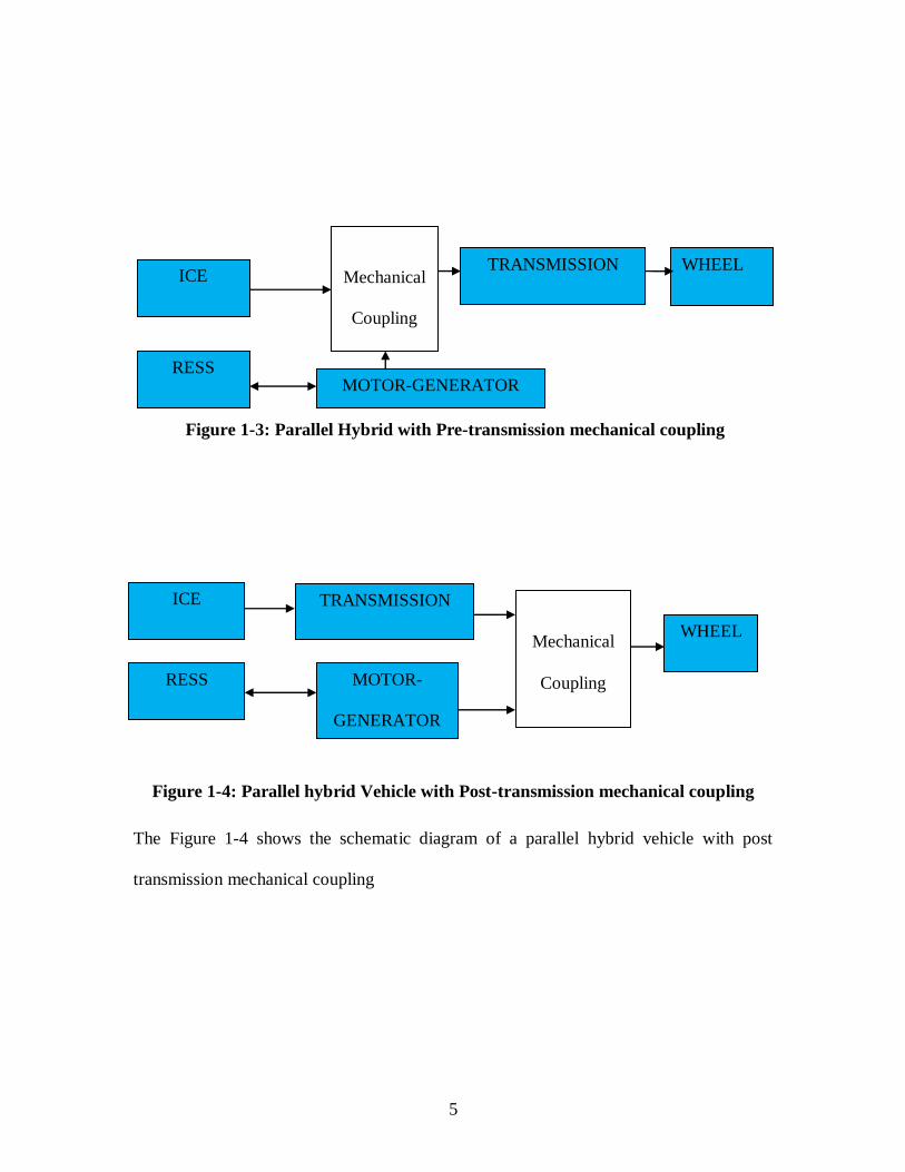
Figure 1-4: Parallel hybrid Vehicle with Post-transmission mechanical coupling

The Figure 1-4 shows the schematic diagram of a parallel hybrid vehicle with post

transmission mechanical coupling

ICE

TRANSMISSION

MOTOR-

GENERATOR

RR

RESS

WHEEL

Mechanical

Coupling

Figure 1-3: Parallel Hybrid with Pre-transmission mechanical coupling

Mechanical

Coupling

TRANSMISSION

WHEEL

ICE

RESS

MOTOR-GENERATOR

6

Figure 1-5: Power Flow in pre-transmission mechanical coupling[3]

Figure 1-6: Power Flow post-transmission mechanical coupling[3]

The Figure 1-5 and Figure 1-6 represent power flow in parallel hybrid electric vehicle

with pre-transmission and post-transmission mechanical coupling[3].

1.3.3 Power-Split Configuration:

A power split hybrid combines the operation of both Series and parallel

configurations. This follows two paths out of which one path is the parallel path and the

other series path. The power split in a power split hybrid vehicle is mainly dependent on

the power split device ( i.e., the planetary gear set).

The advantage of the power-split configuration lies in the fact that the engine

speed can be decoupled from the vehicle speed and hence the engine can be operated at

maximum efficiency points[1] This helps in improving fuel economy and reducing

emissions.

Fuel ICE

RESS EM

+

+

TRANSMISSION

Wheel

Wheel

Fuel ICE

RESS EM

+

+

TRANSMISSION

𝑃𝑟𝑒𝑞

𝑃𝑓𝑐

𝑃𝑒𝑙

𝑃𝑒𝑙

𝑃𝑓𝑐 𝑃𝑖𝑐𝑒 𝑃𝑟𝑒𝑞

7

Figure 1-7: Schematic representation of a power-split Hybrid electric vehicle

The power flow diagram can be represented as follows

Figure 1-8: The Power flow diagram in a power-split hybrid [3]

Fuel

RESS

+

+

ICE

ISA

TRANSMISSION

EM

+

+

+

Wheel

ICE

Planetary

Gear set

WHEEL

MOTOR-

GENERATOR(MG2)

MOTOR-

GENERATOR(MG1)

RESS

𝑃𝑟𝑒𝑞

𝑃𝑒𝑙

𝑃𝑖𝑐𝑒

𝑃𝑒𝑙

8

1.4 Power Split Device

The main component of a power split hybrid electric vehicle is the power split

device known as Planetary gear set. The dynamics of the power split depend on this

planetary gear set. The planetary gear set incorporates a special power transmission

system known as Planetary Gear System, or popularly known as Power Split Device

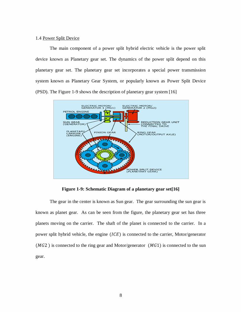
(PSD). The Figure 1-9 shows the description of planetary gear system [16]

Figure 1-9: Schematic Diagram of a planetary gear set[16]

The gear in the center is known as Sun gear. The gear surrounding the sun gear is

known as planet gear. As can be seen from the figure, the planetary gear set has three

planets moving on the carrier. The shaft of the planet is connected to the carrier. In a

power split hybrid vehicle, the engine (𝐼𝐶𝐸) is connected to the carrier, Motor/generator

(𝑀𝐺2 ) is connected to the ring gear and Motor/generator (𝑀𝐺1) is connected to the sun

gear.

9

Figure 1-10: Schematic layout of power-train of a Power split HEV[by Toyota

corporation]

The figure above depicts the way in which the two motor/generators and the

engine are connected in a Power split device [14]. Motor/Generator (𝑀𝐺2) is connected

to the ring gear, which in turn is connected to the final transmission. The engine (𝐼𝐶𝐸) is

connected to the ring gear through planets, and the fraction of torque provided by the

engine to the ring gear depends on the number of teeth of each gear. The speed

relationship between the constitutive elements of the planetary gear set is shown below.

MG1: Motor/Generator connected to the sun-gear in the planetary gear set

predominantly used as generator

MG2: Motor/Generator connected to the ring-gear in the planetary gear set

predominantly used as motor.

As a result of mechanical linkage between the components, the speed relationship

between the components of planetary gear set can be written as

10

(𝝎𝑴𝑮𝟏. 𝑺 + 𝝎𝑴𝑮𝟐.𝑹) = 𝝎𝒊𝒄𝒆 𝑹 + 𝑺 (𝟏.𝟏)

Where

S= No of teeth on sun-gear

R=No of teeth on ring gear

Taking the values as per the configuration of Toyota Prius, we have

S= 30 and R=78

Substituting in the above equation we get

𝟑.𝟔.𝝎𝒊𝒄𝒆 − 𝟐.𝟔.𝝎𝑴𝑮𝟐 = 𝝎𝑴𝑮𝟏 (𝟏.𝟐)

𝝎𝑴𝑮𝟐 = 𝑵𝒇.𝝎𝒘𝒉𝒆𝒆𝒍 (𝟏.𝟑)

Where

𝑁𝑓 = 𝑓𝑖𝑛𝑎𝑙 𝑡𝑟𝑎𝑛𝑠𝑚𝑖𝑠𝑠𝑖𝑜𝑛 𝑟𝑎𝑡𝑖𝑜

𝜔𝑀𝐺2 = 𝐴𝑛𝑔𝑢𝑙𝑎𝑟 𝑣𝑒𝑙𝑜𝑐𝑖𝑡𝑦 𝑜𝑓 𝑀𝐺2

𝜔𝑀𝐺1 = 𝐴𝑛𝑔𝑢𝑙𝑎𝑟 𝑣𝑒𝑙𝑜𝑐𝑖𝑡𝑦 𝑜𝑓 𝑀𝐺1

𝜔𝑤𝑕𝑒𝑒𝑙 = 𝐴𝑛𝑔𝑢𝑙𝑎𝑟 𝑣𝑒𝑙𝑜𝑐𝑖𝑡𝑦 𝑜𝑓 𝑤𝑕𝑒𝑒𝑙

𝜔𝑖𝑐𝑒 = 𝐸𝑛𝑔𝑖𝑛𝑒 𝑆𝑝𝑒𝑒𝑑

In a power-split hybrid electric vehicle, the vehicle can function in different

modes (Figure 1-8) such as parallel pre-transmission mode (ICE+ISA), parallel post-

transmission mode (ICE+EM), series mode (ICE+ISA in regeneration mode and EM in

motoring mode) [3]. All these configurations follow the basic power balance equation

𝑷𝒓𝒆𝒒 𝒕 = 𝑷𝒇𝒄 𝒕 + 𝑷𝒆𝒍 𝒕 (𝟏.𝟒)

Where

11

𝑃𝑓𝑐 = 𝑃𝑜𝑤𝑒𝑟 𝑝𝑟𝑜𝑣𝑖𝑑𝑒𝑑 𝑏𝑦 𝑡𝑕𝑒 𝑓𝑢𝑒𝑙 𝑐𝑜𝑛𝑣𝑒𝑟𝑡𝑒𝑟

𝑃𝑒𝑙 = 𝑃𝑜𝑤𝑒𝑟 𝑝𝑟𝑜𝑣𝑖𝑑𝑒𝑑 𝑏𝑦 𝑡𝑕𝑒 𝑒𝑙𝑒𝑐𝑡𝑟𝑖𝑐𝑎𝑙 𝑎𝑐𝑐𝑢𝑚𝑢𝑙𝑎𝑡𝑜𝑟

𝑃𝑟𝑒𝑞 = 𝑃𝑜𝑤𝑒𝑟 𝑟𝑒𝑞𝑢𝑒𝑠𝑡 𝑎𝑡 𝑡𝑕𝑒 𝑑𝑟𝑖𝑣𝑒𝑟

In the present research, for a power split hybrid as shown in Figure 1-10 ISA is

treated as MG1 connected to the sun gear of the planetary gear set. EM is treated as MG2

connected to the ring gear of the planetary gear set and the speed of the ring gear is same

as the speed of the drive axle.

𝑷𝒆𝒍 = 𝑷𝒆𝒍𝟏 + 𝑷𝒆𝒍𝟐 = 𝑷𝑴𝑮𝟐 − 𝑷𝑴𝑮𝟏 (𝟏.𝟓)

𝑃𝑀𝐺2 > 0 𝑀𝑜𝑡𝑜𝑟 𝑀𝑜𝑑𝑒 ,𝑃𝑀𝐺2 < 0 𝑔𝑒𝑛𝑒𝑟𝑎𝑡𝑜𝑟 𝑚𝑜𝑑𝑒

𝑃𝑀𝐺1 > 0 𝐺𝑒𝑛𝑒𝑟𝑎𝑡𝑜𝑟 𝑚𝑜𝑑𝑒 ,𝑃𝑀𝐺1 < 0(𝑀𝑜𝑡𝑜𝑟 𝑚𝑜𝑑𝑒)

1.5 Plug-in Hybrid Electric Vehicle:

A plug-in hybrid electric vehicle is different from the normal hybrid electric

vehicle. The difference lies in the fact that a plug-in hybrid electric vehicle can use the

stored energy during the charge-depleting operation. This use of electrical energy can

save considerable amount of fuel. PHEVs use lesser fuel than the conventional HEVs

because of the fact that there is a provision for off-board charging of the vehicle. PHEVs

enjoy the same benefits as conventional HEVs and also provide an opportunity for

switching between fuel and electricity- obtaining some of the energy through a charging

plug, which would otherwise be obtained from fuel [20, 21]. Different configurations

exist in Plug-in hybrid electric vehicle and these are more or less similar to the Hybrid

electric vehicle configuration.

12

Since the Plug-in hybrid electric vehicle has the facility of off-board charging, the

vehicle enjoys the benefits of being operated in a charge depletion mode ( with the engine

turned on in the event of high power demand only) until the State of charge of the RESS

reaches a particular value. This not only helps in reducing the fuel costs, but also helps in

reducing the tailpipe emissions. If the vehicle is operated in charge depleting over the

whole trip (with engine not turned on), the vehicle records zero tailpipe emissions.

1.6 Contributions

The thesis focuses on design and optimization of a power split plug-in hybrid

electric vehicle. The dissertation deals with the implementation of instantaneous fuel

consumption strategy viz. ECMS in the backward and forward modeling of a power split

plug-in hybrid electric vehicle. The following tasks have been accomplished in the

research.

A backward facing Quasi-static model of the power split plug-in hybrid electric

vehicle has been developed and the control strategy has been implemented to

minimize the instantaneous fuel consumption of the vehicle.

A supervisory controller(s-function) is used in the optimization and this the

supervisory controller decides the optimal power split between the actuators that

minimizes the fuel consumption.

13

The vehicle is operated in charge-depleting and charge-sustaining operation and

the minimization principle is implemented to maintain the state of charge within a

narrow band in the charge sustenance range.

Similarly a forward facing dynamic model of the power split plug-in hybrid

electric vehicle has been developed and the control strategy is implemented to

minimize the instantaneous fuel consumption of the vehicle.

Unlike the backward model, the forward model considers the engine dynamics

and it includes a driver and vehicle dynamics block that depicts a real time

scenario.

The driver block decides the current power demand based on the throttle

commands generated by the PID controller.

The forward model includes an engine dynamics block that calculates the engine

speed based on the power output from the supervisory controller.

Each subsystem of the actuator is then given the power output from the

supervisory controller as inputs to calculate the efficiencies and real power

outputs based on the maps( if in any case they cross the maximum power output).

The fuel consumption is minimized based on the power output from the

supervisory controller and using the minimization principle.

The fuel consumption is simulated for city and highway cycles and the fuel

economy is maximized by tuning the parameters used in ECMS.

14

1.7 Organization of Thesis

The thesis is organized in the following way.

The first chapter deals with providing insight into the concept of Hybrid electric

vehicle and goes about with explaining different configurations in hybrid electric

vehicles. It also explains about the Plug-in hybrid electric vehicle and power split device

which forms the heart of a power-split hybrid electric vehicle.

The second chapter begins by describing backward and forward modeling

techniques and its differences. Then it describes the higher level model architecture of

both backward and forward models of a plug-in hybrid electric vehicle. The higher level

model architecture is then presented along with modeling of individual components.

The third chapter deals with the power management strategies used in the hybrid

vehicles and goes about by explaining different power management strategies. It also

starts by explaining the local optimization strategy as a local or instantaneous

optimization technique used in the research. The basic differences between global

optimization and local optimization are explained and it mentions how we can use ECMS

in real time applications.

The fourth chapter deals with the implementation of the ECMS strategies in both

forward and backward modeling approaches. The equations used to formulate ECMS for

both these models have been described. The fourth chapter forms the core of the thesis as

it forms the basis for the optimization technique used in the modeling. Both the models

have been studied for fuel consumption. This also presents the differences between

Global and instantaneous minimization approaches. The fourth chapter presents the

15

results produced by implementation of fuel consumption strategy and these results are

produced for both models for city and highway cycles

Fifth chapter deals with conclusions and future work that can be done with regard

to optimization using ECMS.

16

CHAPTER TWO:MODELING APPROACHES IN MODELING OF POWER-TRAINS

2.1 BACKWARD AND FORWARD MODELING OF POWER-TRAINS

2.1.1 Higher level architecture of a backward model

Any power-train can be modeled in two ways, backward and forward modeling.

Backward Model, as the name indicates proceeds backward from the wheels of the

vehicle. This is accomplished by having a driving cycle, and it basically assumes that the

vehicle follows the velocity prescribed by the drive cycle. The power demand at the

wheels is directly calculated from the driving cycle and this power demand is traced back

through the power-train to find out the power split between each individual component.

The backward model has an inherent assumption that the vehicle always follows the

velocity pattern dictated by the driving cycle and hence removes the need of having a

driver model. The following flow diagram illustrates the basic power flow in a backward

model. The input from the drive cycle to the vehicle dynamics block is usually the force

that is computed by comparing the current velocity and the velocity at the next time step

derived from the driving cycle.

Figure 2-1: Higher level architecture of a backward Model

INPUT TORQUE

SPEED

DRIVE

CYCLE

VEHICLE

DYNAMICS

POWERTRAIN

17

The Schematic layout of the power flow inside the power-train of a backward

model is presented in the following figure. The Figure 2-2 shows the layout for the

model used in the present research, i.e. power-split plug-in hybrid electric vehicle.

Figure 2-2: Power flow in a backward model

SPEED INPUT

POWER

SPEED

TORQUE TORQUE

SPEED SPEED TORQUE

POWER

POWER

POWER

SOC

POWER

SPEED

Power-train

RESS (battery)

Motor/Generator

(MG2)

Motor/Generator

(MG1)

HIGHER LEVEL SUPERVISORY CONTROLLER

(OPTIMAL POWER SPLIT)

ICE

Drive Cycle Vehicle

Dynamics

TORQUE

18

The Power flow in a backward model architecture is shown in the Figure 2-2. The

power flow proceeds from the power at the wheels. As mentioned, the backward model

does not have a driver block and the power at the wheels is computed from the drive

cycle. This power at the wheels is translated into the power request at the higher level

supervisory controller (S-function in the present research). The higher level controller

computes the optimal power split based on the power demand at the wheels. The

controller includes the mathematical equations that are required to simulate the optimal

power split in a power-split architecture. The control inputs used in the present research

are the

Power of the motor/generator(MG1 and MG2)

Power of the engine

Power of generator

The controller inputs are manipulated to get the optimal power split that

minimizes the equivalent fuel consumption as dictated by Equivalent fuel Consumption

Strategy which will be discussed in chapters 3 and 4. The higher level uses the current

vehicle speed, engine speed and State of charge of the RESS (battery) as the states based

on which the controller decides the optimal power split. The basis architecture of

backward model neglects faster dynamics and hence the dynamics of components are

neglected. The basic power balance equation is modeled in the following way.

𝑷𝒓𝒆𝒒 𝒕 = 𝑷𝒇𝒄 𝒕 + 𝑷𝒆𝒍 𝒕 (𝟐.𝟏)

Where

𝑃𝑟𝑒𝑞 𝑡 = 𝑃𝑜𝑤𝑒𝑟 𝑟𝑒𝑞𝑢𝑒𝑠𝑡 𝑎𝑡 𝑡𝑕𝑒 𝑤𝑕𝑒𝑒𝑙𝑠 𝑓𝑟𝑜𝑚 𝑣𝑒𝑕𝑖𝑐𝑙𝑒 𝑑𝑦𝑛𝑎𝑚𝑖𝑐𝑠

19

𝑃𝑓𝑐 (𝑡) = 𝑃𝑜𝑤𝑒𝑟 𝑓𝑟𝑜𝑚 𝑡𝑕𝑒 𝑓𝑢𝑒𝑙 𝑐𝑜𝑛𝑣𝑒𝑟𝑡𝑒𝑟 𝐼𝐶𝐸

𝑃𝑒𝑙 𝑡 = 𝑃𝑜𝑤𝑒𝑟 𝑜𝑓 𝑡𝑕𝑒 𝑒𝑙𝑒𝑐𝑡𝑟𝑖𝑐 𝑚𝑎𝑐𝑕𝑖𝑛𝑒𝑠(𝑃𝑀𝐺2 − 𝑃𝑀𝐺1)

𝑃𝑀𝐺1 = 𝑃𝑜𝑤𝑒𝑟 𝑜𝑓 𝑀𝑜𝑡𝑜𝑟/ 𝑔𝑒𝑛𝑒𝑟𝑎𝑡𝑜𝑟 (𝑀𝐺1)[Mechanical]

𝑃𝑀𝐺2 = 𝑃𝑜𝑤𝑒𝑟 𝑜𝑓 𝑀𝑜𝑡𝑜𝑟/ 𝑔𝑒𝑛𝑒𝑟𝑎𝑡𝑜𝑟 (𝑀𝐺2) [Mechanical]

We do not include any dynamics in this modeling pattern and hence assume that

the power demand from the vehicle dynamics is always met and the controller decides the

optimal split based on this power balance equation and the instantaneous fuel

minimization principle (ECMS) which will be discussed in chapters 3 and 4.

2.1.2 Higher level architecture of a forward model

Forward model on the other hand is a bit more realistic and can be applied to a

real time environment. As the name indicates it proceeds forward from the drive train. It

includes a driver model which calculates the error in the velocity by tracking the current

speed and the speed the velocity has to follow. This error is translated into throttle and

brake commands which then calculate the power demand. This power demand is given

as an input to the controller to decide the power split between the actuators. This power

coming out of the actuators goes through the whole power-train to the wheels. The only

difference lies in the fact that the forward model includes a driver block which calculates

the power demand unlike in the backward model where it is directly calculated from the

drive cycle. The schematic layout of a forward model is presented in the following

Figure 2-3.

20

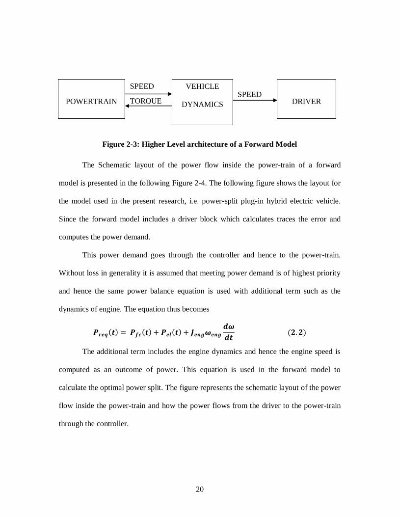
Figure 2-3: Higher Level architecture of a Forward Model

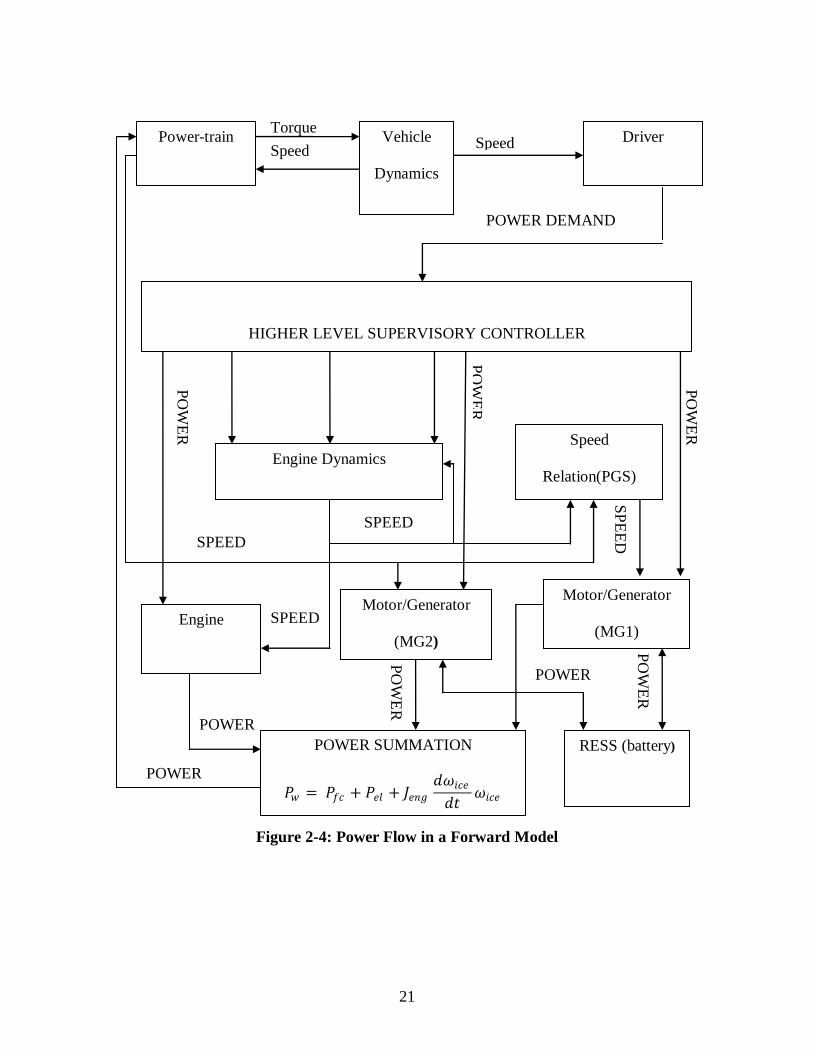
The Schematic layout of the power flow inside the power-train of a forward

model is presented in the following Figure 2-4. The following figure shows the layout for

the model used in the present research, i.e. power-split plug-in hybrid electric vehicle.

Since the forward model includes a driver block which calculates traces the error and

computes the power demand.

This power demand goes through the controller and hence to the power-train.

Without loss in generality it is assumed that meeting power demand is of highest priority

and hence the same power balance equation is used with additional term such as the

dynamics of engine. The equation thus becomes

𝑷𝒓𝒆𝒒 𝒕 = 𝑷𝒇𝒄 𝒕 + 𝑷𝒆𝒍 𝒕 + 𝑱𝒆𝒏𝒈𝝎𝒆𝒏𝒈

𝒅𝝎

𝒅𝒕 (𝟐.𝟐)

The additional term includes the engine dynamics and hence the engine speed is

computed as an outcome of power. This equation is used in the forward model to

calculate the optimal power split. The figure represents the schematic layout of the power

flow inside the power-train and how the power flows from the driver to the power-train

through the controller.

SPEED

POWERTRAIN

VEHICLE

DYNAMICS

DRIVER

SPEED

TORQUE

21

Figure 2-4: Power Flow in a Forward Model

Motor/Generator

(MG1)

Motor/Generator

(MG2)

RESS (battery)

Engine Dynamics

Speed

Relation(PGS)

𝑃𝑤 = 𝑃𝑓𝑐 + 𝑃𝑒𝑙 + 𝐽𝑒𝑛𝑔𝑑𝜔𝑖𝑐𝑒

𝑑𝑡𝜔𝑖𝑐𝑒

POWER SUMMATION

HIGHER LEVEL SUPERVISORY CONTROLLER

(OPTIMAL POWER SPLIT)

Engine

Power-train

Driver

Vehicle

Dynamics

SPEED

SPEED P

OW

ER

PO

WE

R

POWER DEMAND

PO

WE

R

SP

EE

D

SPEED

POWER

POWER

POWER

PO

WE

R

PO

WE

R

Speed Speed

Torque

22

2.1.3 Modeling of Components

2.1.3.1 Modeling of Engine

The engine is modeled as the following representation. Although the engine fuel

consumption, torque and power maps are embedded inside the s-function (supervisory

controller), the Figure 2-4 just emphasizes on having them outside to give a deeper

insight into the basic backward model architecture. Since the backward model neglects

the dynamics of individual components (actuators), it becomes easier just to have a

supervisory controller which that calculates the optimal power split that minimizes the

fuel consumption. The engine power in the backward model is calculated inside the

supervisory controller based on the power request at wheels and also based on the states

of the system such as current engine speed, state of charge of SOC and vehicle speed.

This optimal engine power is used to calculate optimal fuel consumption based on the

fuel consumption maps. The representation of engine modeling inside the Supervisory

controller is shown below. Given the power demand (the torque and the optimal speed

dictated by the supervisory controller), we can find the fuel consumption of the engine

from the specific fuel consumption map. This fuel consumption is the optimal fuel

consumption for the optimal power split. This is represented in the Figure 2-5.

23

Figure 2-5: Information flow to engine in a backward model

Though the basic modeling of the engine is same in the forward modeling approach, it

becomes imperative to have these subsystems as individual components outside the

supervisory controller, replicating a real time environment. Added to this, the forward

model, as seen from the perspective of modeling a real time system, it becomes

imperative that one has the dynamics included in the model. Hence the supervisory

controller in the forward model includes the dynamics in the basic energy or power

conservation equation that decides the power split. Since the supervisory controller is

triggered each second, the dynamics included here are inherently changing each second

and to avoid this we place a real time dynamics block that happen at a faster rate. The

basic power balance equation, with the dynamics included, used in the forward model

helps us in finding the real engine speed, which along with the toque output from the

supervisory controller, is sent to the engine subsystem to calculate the real torque output

based on the steady-state engine maps.

.

ICE

Supervisory

Controller

TORQUE

SPEED

Fuel Consumption 𝑚 𝑓

24

Figure 2-6: Information flow to engine in a forward model

The Figure 2-6 represents the representation of the engine in a forward model

2.1.3.2 Modeling of Motor/generator Subsystems

In the configuration used in the research, we have two motor/generators (MG1

and MG2) attached to the power split device (planetary gear set), Figure 1-10 The

modeling of these motor/generators is same in both forward and backward modeling

approaches.

The only difference lies in the fact that the motor and generator sets used in the

backward model assume that these sets provide the power dictated by the controller.

Although this is true most of the times in the forward model, it becomes necessary to

check for the maximum torque or power limitations having the subsystems outside since

the forward model depicts a real time system with the dynamics changing at a faster rate

than the backward model where the whole system runs at a finite time step. The

backward configuration also has them outside the supervisory controller just to calculate

ICE

Engine

Dynamics

Supervisory

Controller

Torque

Speed

Fuel Consumption 𝑚 𝑓

25

the efficiency losses and hence the power going in/coming out of the Renewable

Electrical storage system (RESS or Battery). The representation of each of the

Motor/generator sets in backward model is shown in Figure 2-7.

Figure 2-7: Information flow to motor/generator in a backward model

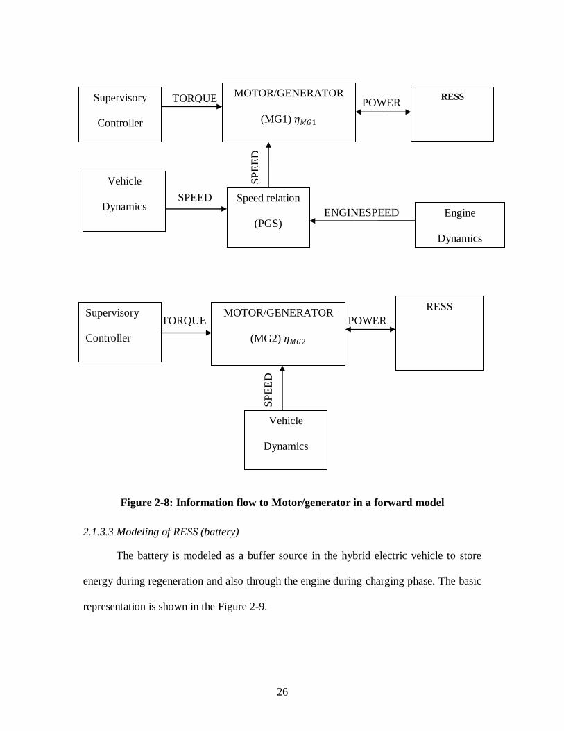
In the forward model, the representation is slightly different. The Figure 2-8

below shows the representation of two motor/generator sets used in the power split

configuration.

MOTOR/GENERATOR

(MG1) 𝜂𝑀𝐺1

Supervisory

Controller

RESS

SPEED

TORQUE

POWER

MOTOR/GENERATOR

(MG2) 𝜂𝑀𝐺2

Supervisory

Controller

RESS

SPEED

TORQUE

26

Figure 2-8: Information flow to Motor/generator in a forward model

2.1.3.3 Modeling of RESS (battery)

The battery is modeled as a buffer source in the hybrid electric vehicle to store

energy during regeneration and also through the engine during charging phase. The basic

representation is shown in the Figure 2-9.

MOTOR/GENERATOR

(MG1) 𝜂𝑀𝐺1

Speed relation

(PGS)

Supervisory

Controller

Vehicle

Dynamics

RESS

Engine

Dynamics

SPEED

TORQUE

ENGINESPEED

POWER

SP

EE

D

MOTOR/GENERATOR

(MG2) 𝜂𝑀𝐺2

Vehicle

Dynamics

(PGS)

Supervisory

Controller

RESS

TORQUE POWER

SP

EE

D

27

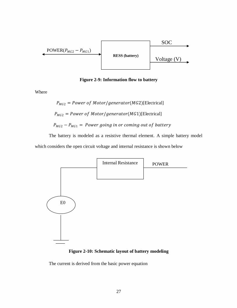
Figure 2-9: Information flow to battery

Where

𝑃𝑀𝐺2 = 𝑃𝑜𝑤𝑒𝑟 𝑜𝑓 𝑀𝑜𝑡𝑜𝑟/𝑔𝑒𝑛𝑒𝑟𝑎𝑡𝑜𝑟(𝑀𝐺2)[Electrical]

𝑃𝑀𝐺2 = 𝑃𝑜𝑤𝑒𝑟 𝑜𝑓 𝑀𝑜𝑡𝑜𝑟/𝑔𝑒𝑛𝑒𝑟𝑎𝑡𝑜𝑟(𝑀𝐺1)[Electrical]

𝑃𝑀𝐺2 − 𝑃𝑀𝐺1 = 𝑃𝑜𝑤𝑒𝑟 𝑔𝑜𝑖𝑛𝑔 𝑖𝑛 𝑜𝑟 𝑐𝑜𝑚𝑖𝑛𝑔 𝑜𝑢𝑡 𝑜𝑓 𝑏𝑎𝑡𝑡𝑒𝑟𝑦

The battery is modeled as a resistive thermal element. A simple battery model

which considers the open circuit voltage and internal resistance is shown below

Figure 2-10: Schematic layout of battery modeling

The current is derived from the basic power equation

Internal Resistance

E0

RESS (battery)

POWER(𝑃𝑀𝐺2 − 𝑃𝑀𝐺1)

SOC

Voltage (V)

POWER

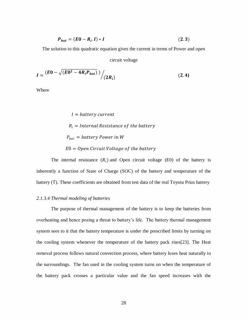
28

𝑷𝒃𝒂𝒕 = 𝑬𝟎 − 𝑹𝒊. 𝑰 ∗ 𝑰 (𝟐.𝟑)

The solution to this quadratic equation gives the current in terms of Power and open

circuit voltage

𝑰 =(𝑬𝟎− (𝑬𝟎𝟐 − 𝟒𝑹𝒊𝑷𝒃𝒂𝒕) )

(𝟐𝑹𝒊) (𝟐.𝟒)

Where

𝐼 = 𝑏𝑎𝑡𝑡𝑒𝑟𝑦 𝑐𝑢𝑟𝑟𝑒𝑛𝑡

𝑅𝑖 = 𝐼𝑛𝑡𝑒𝑟𝑛𝑎𝑙 𝑅𝑒𝑠𝑖𝑠𝑡𝑎𝑛𝑐𝑒 𝑜𝑓 𝑡𝑕𝑒 𝑏𝑎𝑡𝑡𝑒𝑟𝑦

𝑃𝑏𝑎𝑡 = 𝑏𝑎𝑡𝑡𝑒𝑟𝑦 𝑃𝑜𝑤𝑒𝑟 𝑖𝑛 𝑊

𝐸0 = 𝑂𝑝𝑒𝑛 𝐶𝑖𝑟𝑐𝑢𝑖𝑡 𝑉𝑜𝑙𝑡𝑎𝑔𝑒 𝑜𝑓 𝑡𝑕𝑒 𝑏𝑎𝑡𝑡𝑒𝑟𝑦

The internal resistance (𝑅𝑖) and Open circuit voltage (E0) of the battery is

inherently a function of State of Charge (SOC) of the battery and temperature of the

battery (T). These coefficients are obtained from test data of the real Toyota Prius battery

2.1.3.4 Thermal modeling of batteries

The purpose of thermal management of the battery is to keep the batteries from

overheating and hence posing a threat to battery’s life. The battery thermal management

system sees to it that the battery temperature is under the prescribed limits by turning on

the cooling system whenever the temperature of the battery pack rises[23]. The Heat

removal process follows natural convection process, where battery loses heat naturally to

the surroundings. The fan used in the cooling system turns on when the temperature of

the battery pack crosses a particular value and the fan speed increases with the

29

temperature. The battery controller decides this speed based on the temperature. The

temperature of the battery is basically modeled according to the following equation.

𝑻𝒃𝒂𝒕 = (𝑸𝒊𝒏 − 𝑸𝒐𝒖𝒕)𝒕

𝟎𝒅𝒕

𝒎𝑪𝒑 (𝟐.𝟓)

It is the integral of the difference between the heat going into the battery and heat

exchanged between the battery and ambient air.

Where

𝑄𝑖𝑛 = 𝐻𝑒𝑎𝑡 𝑝𝑟𝑜𝑑𝑢𝑐𝑒𝑑 𝑑𝑢𝑒 𝑡𝑜 𝑡𝑕𝑒 𝑐𝑢𝑟𝑟𝑒𝑛𝑡 𝑖𝑛𝑠𝑖𝑑𝑒 𝑡𝑕𝑒 𝑏𝑎𝑡𝑡𝑒𝑟𝑦 𝐽𝑜𝑢𝑙𝑒 ′𝑒𝑓𝑓𝑒𝑐𝑡

𝑄𝑜𝑢𝑡 = 𝐻𝑒𝑎𝑡 𝑙𝑜𝑠𝑡 𝑑𝑢𝑒 𝑡𝑜 𝑐𝑜𝑛𝑣𝑒𝑐𝑡𝑖𝑜𝑛 𝑏𝑒𝑡𝑤𝑒𝑒𝑛 𝑡𝑕𝑒 𝑏𝑎𝑡𝑡𝑒𝑟𝑦 𝑎𝑛𝑑 𝑠𝑢𝑟𝑟𝑜𝑢𝑛𝑑𝑖𝑛𝑔𝑠

𝑸𝒐𝒖𝒕 = (𝑻𝒃𝒂𝒕 − 𝑻𝒂𝒎𝒃) 𝟏 +

𝒖𝟐

𝒉𝑨

𝒎𝑪𝒑 (𝟐.𝟔)

Where

(𝑕𝐴).𝑁.𝑝𝑎𝑐𝑘𝑠 = 𝐸𝑓𝑓𝑒𝑐𝑡𝑖𝑣𝑒 𝑐𝑜𝑛𝑣𝑒𝑐𝑡𝑖𝑣𝑒 𝑕𝑒𝑎𝑡 𝑡𝑟𝑎𝑛𝑠𝑓𝑒𝑟 𝑓𝑜𝑟 𝑡𝑕𝑒 𝑏𝑎𝑡𝑡𝑒𝑟𝑦

𝑚𝐶𝑝 .𝑁.𝑝𝑎𝑐𝑘𝑠 = 𝑇𝑕𝑒𝑟𝑚𝑎𝑙 𝑀𝑎𝑠𝑠 𝑜𝑓 𝑡𝑕𝑒 𝑏𝑎𝑡𝑡𝑒𝑟𝑦

𝑁 = 𝑁𝑢𝑚𝑏𝑒𝑟 𝑜𝑓 𝑐𝑒𝑙𝑙𝑠 𝑖𝑛 𝑠𝑒𝑟𝑖𝑒𝑠

𝑃 = 𝑁𝑢𝑚𝑏𝑒𝑟 𝑜𝑓 𝑝𝑎𝑐𝑘𝑠

𝑕𝐴 = 𝐴𝑣𝑒𝑟𝑎𝑔𝑒 𝑕𝑒𝑎𝑡 𝑡𝑟𝑎𝑛𝑠𝑓𝑒𝑟 𝑜𝑣𝑒𝑟 𝑎 𝑠𝑖𝑛𝑔𝑙𝑒 𝑐𝑒𝑙𝑙 𝑖𝑛 𝑡𝑕𝑒 𝑏𝑎𝑡𝑡𝑒𝑟𝑦 𝑝𝑎𝑐𝑘

𝑇𝑏𝑎𝑡 = 𝑡𝑒𝑚𝑝𝑒𝑟𝑎𝑡𝑢𝑟𝑒 𝑜𝑓 𝑡𝑕𝑒 𝑏𝑎𝑡𝑡𝑒𝑟𝑦

𝑇𝑎𝑚𝑏 = 𝐴𝑚𝑏𝑖𝑒𝑛𝑡 𝑡𝑒𝑚𝑝𝑒𝑟𝑎𝑡𝑢𝑟𝑒

𝑢 = 𝐹𝑎𝑛 𝑠𝑒𝑡𝑡𝑖𝑛𝑔 𝑑𝑒𝑝𝑒𝑛𝑑𝑖𝑛𝑔 𝑢𝑝𝑜𝑛 𝑇𝑏𝑎𝑡

When

𝑇𝑏𝑎𝑡 ≥ 40, 𝑢 𝑖𝑠 𝑠𝑒𝑡 𝑎𝑠 3

30

𝑇𝑏𝑎𝑡 ≥ 35, 𝑢 𝑖𝑠 𝑠𝑒𝑡 𝑎𝑠 2

𝑇𝑏𝑎𝑡 ≥ 30, 𝑢 𝑖𝑠 𝑠𝑒𝑡 𝑎𝑠 1

𝑒𝑙𝑠𝑒

𝑢 𝑖𝑠 𝑠𝑒𝑡 𝑎𝑠 𝑧𝑒𝑟𝑜

This fan setting helps us to control the battery temperature and hence keep the battery

temperature within the prescribed range.

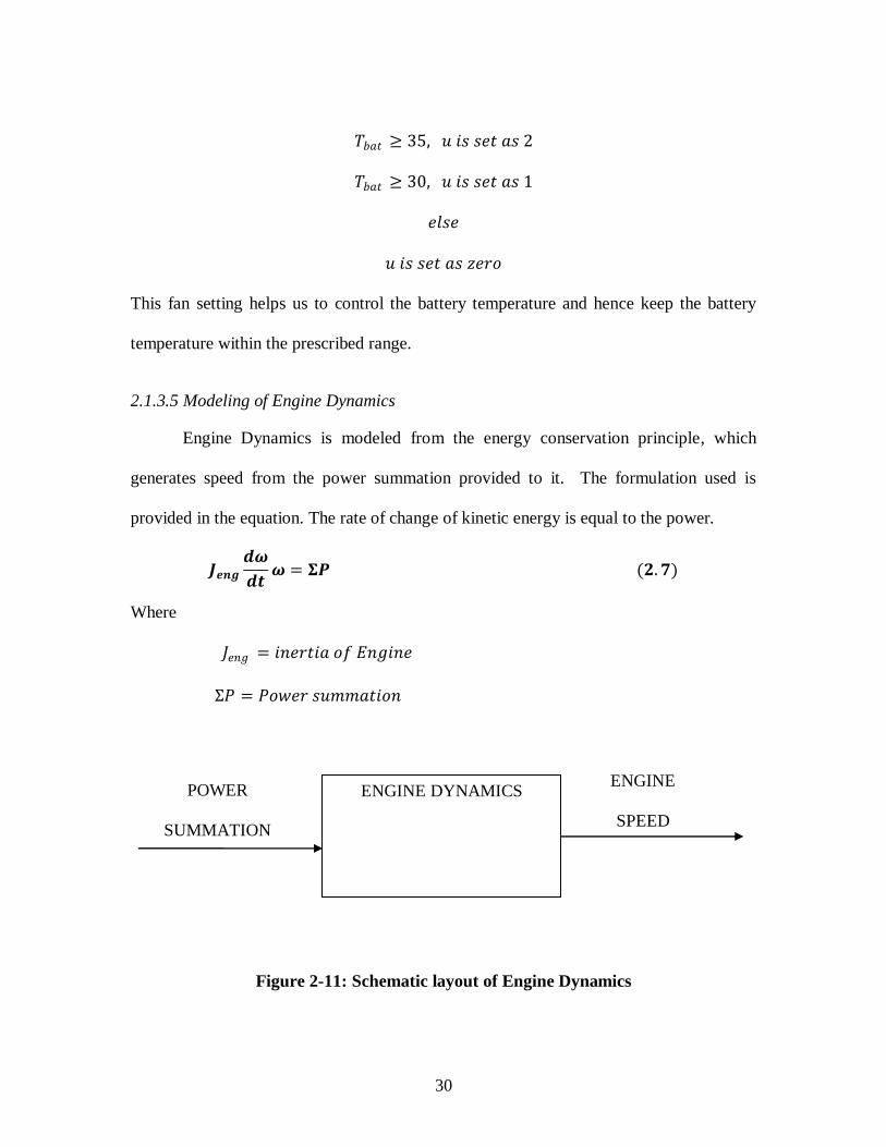
2.1.3.5 Modeling of Engine Dynamics

Engine Dynamics is modeled from the energy conservation principle, which

generates speed from the power summation provided to it. The formulation used is

provided in the equation. The rate of change of kinetic energy is equal to the power.

𝑱𝒆𝒏𝒈𝒅𝝎

𝒅𝒕𝝎 = 𝚺𝑷 (𝟐.𝟕)

Where

𝐽𝑒𝑛𝑔 = 𝑖𝑛𝑒𝑟𝑡𝑖𝑎 𝑜𝑓 𝐸𝑛𝑔𝑖𝑛𝑒

Σ𝑃 = 𝑃𝑜𝑤𝑒𝑟 𝑠𝑢𝑚𝑚𝑎𝑡𝑖𝑜𝑛

Figure 2-11: Schematic layout of Engine Dynamics

ENGINE DYNAMICS POWER

SUMMATION

ENGINE

SPEED

31

2.1.3.6 Modeling of Vehicle Dynamics:

The vehicle dynamics block is modeled according to Newton’s Second law of

motion which states that the net acceleration produced on the body is always the resultant

of the net force acting on the body. The resistive elements acting on the body are the

aerodynamic force, drag force and the rolling resistance between the wheel and the

ground surface. The following equations describe the vehicle dynamics block

𝒎𝒗.𝒅𝒗

𝒅𝒕= 𝑭𝒕𝒓𝒂𝒄𝒕𝒊𝒐𝒏 − 𝑭𝒂 − 𝑭𝒈 − 𝑭𝒓 (𝟐.𝟖)

𝑭𝒂 = 𝝆𝒂𝒊𝒓𝑪𝒅𝑨𝒇𝒗

𝟐

𝟐 (𝟐.𝟗)

𝑭𝒈 = 𝒎𝒗𝒈𝒄𝒐𝒔 𝜶 (𝟐.𝟏𝟎)

𝑭𝒓 = 𝒎𝒗𝒈𝑪𝒓 𝐬𝐢𝐧 𝜶 (𝟐.𝟏𝟏)

𝝎𝒘𝒉𝒆𝒆𝒍 = 𝒗 𝒓𝒘𝒉𝒆𝒆𝒍 (𝟐.𝟏𝟐)

Where

𝐹𝑎 = 𝐴𝑒𝑟𝑜𝑑𝑦𝑛𝑎𝑚𝑖𝑐 𝑓𝑜𝑟𝑐𝑒 𝑎𝑐𝑡𝑖𝑛𝑔 𝑜𝑛 𝑡𝑕𝑒 𝑣𝑒𝑕𝑖𝑐𝑙𝑒 𝑖𝑛 𝑁

𝐹𝑔 = 𝐺𝑟𝑎𝑑𝑒 𝑓𝑜𝑟𝑐𝑒 𝑑𝑢𝑒 𝑡𝑜 𝑎𝑛𝑦 𝑖𝑛𝑐𝑙𝑖𝑛𝑎𝑡𝑖𝑜𝑛 𝑜𝑓 𝑡𝑕𝑒 𝑟𝑜𝑎𝑑 𝑖𝑛 𝑁

𝐹𝑟 = 𝑅𝑜𝑙𝑙𝑖𝑛𝑔 𝑟𝑒𝑠𝑖𝑠𝑡𝑎𝑛𝑐𝑒 𝑏𝑒𝑡𝑤𝑒𝑒𝑛 𝑣𝑒𝑕𝑖𝑐𝑙𝑒 𝑎𝑛𝑑 𝑟𝑜𝑎𝑑 𝑖𝑛 𝑁

𝐶𝑑 = 𝐷𝑟𝑎𝑔 𝐶𝑜𝑒𝑓𝑓𝑖𝑐𝑖𝑒𝑛𝑡

𝐶𝑟 = 𝑅𝑜𝑙𝑙𝑖𝑛𝑔 𝑟𝑒𝑠𝑖𝑠𝑡𝑎𝑛𝑐𝑒 𝑐𝑜𝑒𝑓𝑓𝑖𝑐𝑖𝑒𝑛𝑡

𝐴𝑓 = 𝑉𝑒𝑕𝑖𝑐𝑙𝑒 𝐹𝑟𝑜𝑛𝑡𝑎𝑙 𝑎𝑟𝑒𝑎 𝑖𝑛 𝑚

32

𝜌𝑎𝑖𝑟 = 𝐷𝑒𝑛𝑠𝑖𝑡𝑦 𝑜𝑓 𝑎𝑖𝑟 𝑖𝑛 𝑘𝑔/𝑚3

𝛼 = 𝐼𝑛𝑐𝑙𝑖𝑛𝑎𝑡𝑖𝑜𝑛 𝑜𝑓 𝑡𝑕𝑒 𝑟𝑜𝑎𝑑 𝑠𝑢𝑟𝑓𝑎𝑐𝑒

𝑚𝑣 = 𝑀𝑎𝑠𝑠 𝑜𝑓 𝑡𝑕𝑒 𝑣𝑒𝑕𝑖𝑐𝑙𝑒 𝑖𝑛 𝑘𝑔

𝑔 = 𝐴𝑐𝑐𝑒𝑙𝑒𝑟𝑎𝑡𝑖𝑜𝑛 𝑑𝑢𝑒 𝑡𝑜 𝑔𝑟𝑎𝑣𝑖𝑡𝑦 𝑖𝑛 𝑚 𝑠2

𝑣 = 𝑉𝑒𝑕𝑖𝑐𝑙𝑒 𝑣𝑒𝑙𝑜𝑐𝑖𝑡𝑦 𝑖𝑛 𝑚/𝑠

𝐹𝑡𝑟𝑎𝑐𝑡𝑖𝑜𝑛 = 𝑇𝑟𝑎𝑐𝑡𝑖𝑜𝑛 𝑓𝑜𝑟𝑐𝑒 𝑜𝑛 𝑡𝑕𝑒 𝑣𝑒𝑕𝑖𝑐𝑙𝑒 𝑖𝑛 𝑁

𝜔𝑤𝑕𝑒𝑒𝑙 = 𝐴𝑛𝑔𝑢𝑙𝑎𝑟 𝑣𝑒𝑙𝑜𝑐𝑖𝑡𝑦 𝑜𝑓 𝑡𝑕𝑒 𝑤𝑕𝑒𝑒𝑙 𝑖𝑛 𝑟𝑎𝑑/𝑠

𝑟𝑤𝑕𝑒𝑒𝑙 = 𝑅𝑎𝑑𝑖𝑢𝑠 𝑜𝑓 𝑡𝑕𝑒 𝑤𝑕𝑒𝑒𝑙 𝑖𝑛 𝑚

The traction force creates the basic difference between the forward modeling

approach and backward modeling approach. In a backward model it is assumed that the

traction force is provided from the vehicle dynamics block assuming that the change in

velocity is calculated from the drive cycle. In the forward model the force is the resultant

of torque provided by the power-train and hence the acceleration is computed taking into

account the force provided by the power-train.

2.1.3.7 Modeling of Driver

Driver is modeled as a PID controller which takes in the input as vehicle velocity

and the driving cycle velocity. It calculates the error based of these two and hence

generates a throttle or braking command. These commands are then translated into power

request at the actuators. Driver is used only in the forward modeling approach as the need

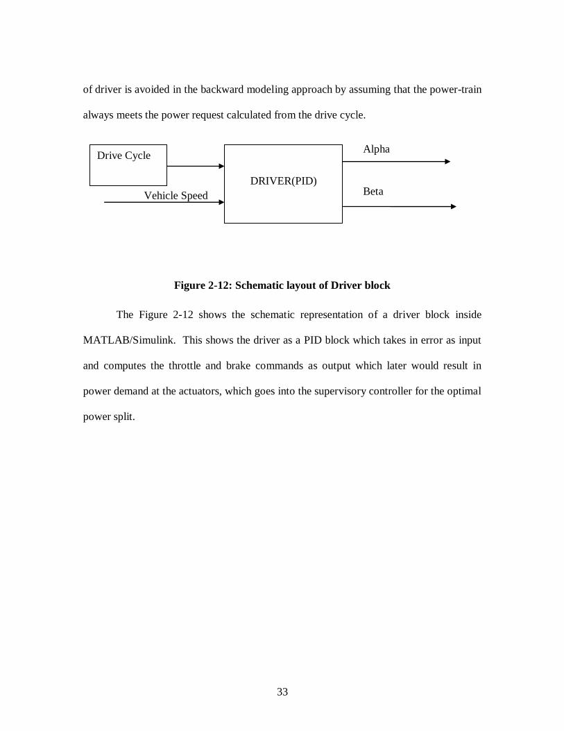
33

of driver is avoided in the backward modeling approach by assuming that the power-train

always meets the power request calculated from the drive cycle.

Figure 2-12: Schematic layout of Driver block

The Figure 2-12 shows the schematic representation of a driver block inside

MATLAB/Simulink. This shows the driver as a PID block which takes in error as input

and computes the throttle and brake commands as output which later would result in

power demand at the actuators, which goes into the supervisory controller for the optimal

power split.

Drive Cycle

DRIVER(PID)

Vehicle Speed

Alpha

Beta

34

CHAPTER THREE: POWER MANAGEMENT IN A HYBRID ELECTRIC VEHICLE

3.1 Modes of Operation

Any plug-in hybrid electric vehicle can be operated in three modes.

Charge Depleting mode

Charge Sustaining mode

Blended mode

3.1.1 Charge Depleting mode:

This mode uses the RESS’ power to the maximum extent. The Engine assists the

motor only during peak power demand or high acceleration. The battery is depleted until

it reaches a particular threshold. The engine assists the vehicle only when the power

required is more than the power of the power that the battery can deliver. The battery is

only charged in the event of regenerative braking. This mode does not use engine or

generator to charge the RESS/battery.

3.1.2 Charge Sustaining mode:

This mode uses both internal combustion engine and RESS simultaneously so that

the state of Charge of the Renewable Energy storage device does is maintained within the

prescribed limits. The prescribed limit is very small and the control strategy sees to it

that the state of charge of the battery does not fall below these limits.

35

The combined operation in these two modes is known as a CDCS strategy,

wherein a vehicle is operated in charge depleting mode initially and when the state of

charge of the RESS falls to a particular value, the charge sustaining mode is activated. In

charge depleting mode, the engine assists the vehicle during high power demands.

3.1.3 Blended Mode

The vehicle can also be operated in blended mode during which the engine can be

triggered more often when compared to the charge depletion operation. This ensures that

the vehicle takes longer time to reach charge sustaining operation.

One advantage that blended operation has when compared to CDCS strategy is

that the by delaying the charge sustenance phase the overall PHEV costs are reduced.

In the charge depleting phase (in plug-in hybrid electric vehicles), the freedom of

operating the engine at higher efficiencies is constrained. Normally a power-split

architecture enjoys the benefits of decoupling the engine and allowing it to run at points

where fuel efficiency is maximum[1], but in charge depleting mode the engine power is

requested only when the power demand cannot be met by the electric machines. Hence

this reduces the freedom of operating the engine at maximum fuel efficient points. In

blended strategy this can be achieved by running the engine more often even if the power

demand can be met by the electric machines alone. This allows for operating the engine

at high efficiency points. This allows for utilization of electric energy over a longer

range in charge depletion mode and hence improving the fuel economy[1].

36

3.2 POWER MANAGEMENT STRATEGIES IN A HYBRID VEHICLE

Hybrid vehicles constitute at least two different power sources. A hybrid power-

train combines the operation of two or more modes of propulsion to achieve better results

when compared to a normal single power-train. This kind of configuration can produce

better results in terms of reduction of fuel consumption and improving fuel economy.

The performance of Hybrid electric vehicle strongly depends on the power split. And

this power split plays a major role in the minimization of fuel consumption. When two or

more power sources are available, the control strategy has to determine optimal power

distribution between the two sources that minimize the fuel economy. The power split is

constrained by two factors: The driver power demand must be met and the State of

Charge of the RESS must be maintained within the prescribed limits. Within these

constraints the motive power must be split to minimize the fuel consumption.

Different Power management strategies have been developed in different configurations

of hybrid electric vehicles.

Rule based techniques

Dynamic Programming

Local Optimization(Equivalent Consumption Minimization strategy)

3.2.1 Rule based strategy

The first technique is the Rule based technique. This control technique is

implemented using heuristic control knowledge to develop a set of event triggered rules.

The decision to operate different actuators depends on a set of parameters like State of

Charge of RESS, power demand from the vehicle, current speed of the internal

37

combustion engine. The rule based control strategy can be designed in such a way that

either of the two actuators i.e. ICE or Motor can act as the main propelling device[

Normally in PHEVs, the motor acts as the main propelling unit, with engine charging the

batteries and assisting the vehicle during high power demand. The other actuator is

activated depending on a set of event triggered rules. This device is generally termed as a

load-leveling device. The engine can also act as the main propelling source with the

RESS acting as a load leveling device [14]. In the present description of the rule based

strategy for a power split plug-in hybrid electric vehicle [11,12,20], we consider Motor

attached to the ring gear as the main propelling device and engine as the secondary

device assisting the motor. The motor is always driving the vehicle, and the decision to

turn on or turn off the engine depends on a set of parameters like State of Charge of

battery, power demand from the vehicle. We can categorize different modes of operation

as

Start: Depending on the power demand during vehicle start, the power can be

split between motor and engine based on certain set of event triggered rules.

Stop: During this phase the vehicle comes to a complete halt and the engine can

be made to run at idle speed or can simply be turned off.

Cruise mode: Normal driving mode without any high acceleration. The power

demand is satisfied by the motor alone if the State of Charge is within the limits (

in charge depletion mode).

Hard Acceleration: The engine provides the additional torque to meet the

torque/power demand.

38

Recharge: When state of charge of the RESS falls below a particular threshold,

engine helps in charging the RESS through generator.

Regeneration: The regenerative braking helps in recuperating kinetic energy.

Hard braking: During this phase, conventional braking is activated to stop the

vehicle.

3.2.2 Dynamic Programming

The second technique is based on Global optimization that is usually presented in

the form of Dynamic Programming. Although rule based strategies helped researchers in

the budding stages of hybrid vehicle research, these strategies were not useful in

minimizing the overall fuel consumption of a hybrid electric vehicle. This necessitated

further research into the strategies that minimize the overall global fuel consumption by

satisfying various physical constraints imposed on the power-train.

Dynamic programming can be referred to as a global optimization strategy.

Dynamic Programming (DP) is a multistage decision making process requiring a

sequence of interrelated decisions [9,10]. Dynamic programming is a recursive approach.

It simplifies by breaking the problem into a set of smaller problems and by combining

them using a recursive approach. For a given system the dynamic programming

approach follows a search algorithm that searches all values of control inputs over state

that has been discritized. Normally in global optimization problem for minimization of

fuel consumption the cost function is the total fuel consumption. Dynamic programming

approach combines different objectives such as minimizing the fuel consumption and

keeping the battery State of Charge sustained. One such constraint is known as hard

39

constraint where final state of charge is equal to the initial state of charge. One can also

use a soft constraint by adding a penalty term that accounts for the deviation of the final

SOC from initial SOC. When a soft constraint is used the global optimization problem

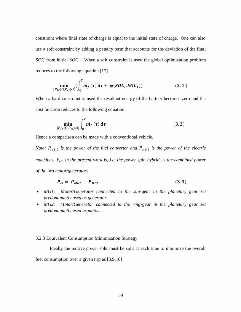
reduces to the following equation [17]

𝐦𝐢𝐧 𝑷𝒇𝒄 𝒕 ,𝑷𝒆𝒍 𝒕

( 𝒎𝒇 𝑻

𝟎

𝝉 𝒅𝝉 + 𝝋(𝑺𝑶𝑪𝒊,𝑺𝑶𝑪𝒇)) (𝟑.𝟏 )

When a hard constraint is used the resultant energy of the battery becomes zero and the

cost function reduces to the following equation.

𝐦𝐢𝐧 𝑷𝒇𝒄 𝒕 ,𝑷𝒆𝒍, 𝒕

𝒎𝒇 𝑻

𝟎

𝝉 𝒅𝝉 (𝟑.𝟐)

Hence a comparison can be made with a conventional vehicle.

Note: 𝑃𝑓𝑐 (𝑡) is the power of the fuel converter and 𝑃𝑒𝑙 (𝑡) is the power of the electric

machines. 𝑃𝑒𝑙 , in the present work is, i.e. the power split hybrid, is the combined power

of the two motor/generators.

𝑷𝒆𝒍 = 𝑷𝑴𝑮𝟐 − 𝑷𝑴𝑮𝟏 (𝟑.𝟑)

MG1: Motor/Generator connected to the sun-gear in the planetary gear set

predominantly used as generator

MG2: Motor/Generator connected to the ring-gear in the planetary gear set

predominantly used as motor.

3.2.3 Equivalent Consumption Minimization Strategy

Ideally the motive power split must be split at each time to minimize the overall

fuel consumption over a given trip as [3,9,10]

40

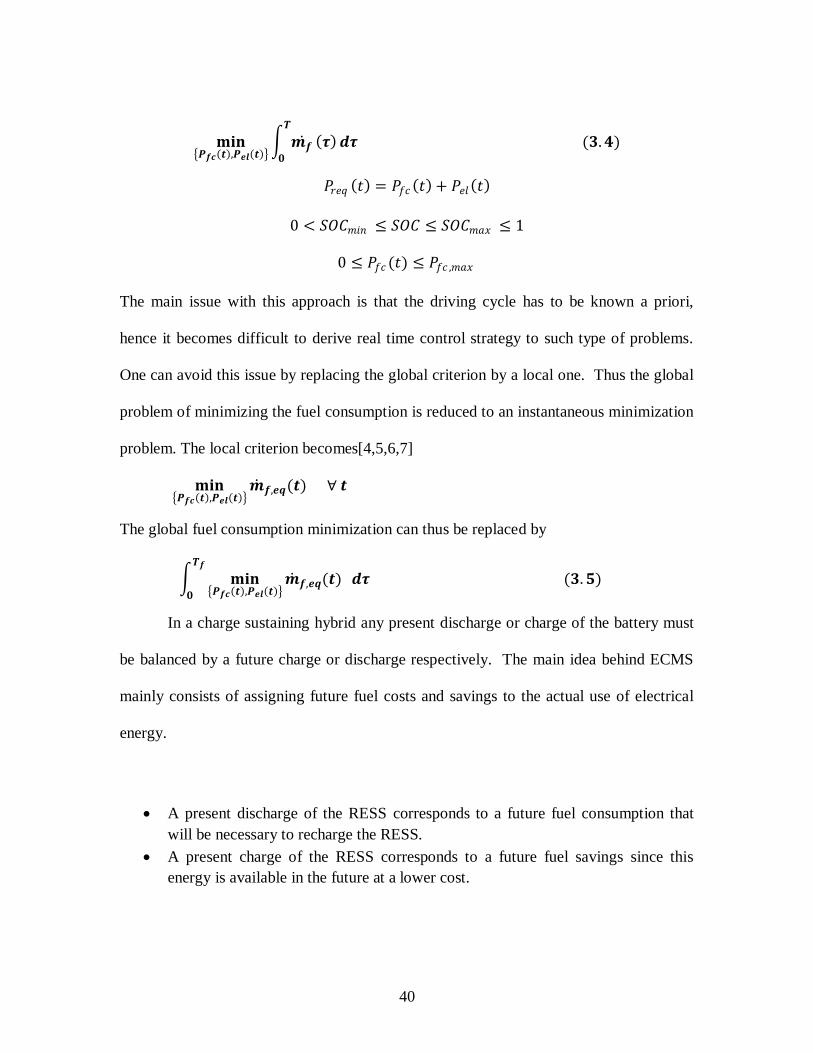
𝐦𝐢𝐧 𝑷𝒇𝒄 𝒕 ,𝑷𝒆𝒍 𝒕

𝒎𝒇 𝑻

𝟎

𝝉 𝒅𝝉 (𝟑.𝟒)

𝑃𝑟𝑒𝑞 𝑡 = 𝑃𝑓𝑐 𝑡 + 𝑃𝑒𝑙 𝑡

0 < 𝑆𝑂𝐶𝑚𝑖𝑛 ≤ 𝑆𝑂𝐶 ≤ 𝑆𝑂𝐶𝑚𝑎𝑥 ≤ 1

0 ≤ 𝑃𝑓𝑐 (𝑡) ≤ 𝑃𝑓𝑐 ,𝑚𝑎𝑥

The main issue with this approach is that the driving cycle has to be known a priori,

hence it becomes difficult to derive real time control strategy to such type of problems.

One can avoid this issue by replacing the global criterion by a local one. Thus the global

problem of minimizing the fuel consumption is reduced to an instantaneous minimization

problem. The local criterion becomes[4,5,6,7]

𝐦𝐢𝐧 𝑷𝒇𝒄 𝒕 ,𝑷𝒆𝒍 𝒕

𝒎 𝒇,𝒆𝒒(𝒕) ∀ 𝒕

The global fuel consumption minimization can thus be replaced by

𝐦𝐢𝐧 𝑷𝒇𝒄 𝒕 ,𝑷𝒆𝒍 𝒕

𝒎 𝒇,𝒆𝒒(𝒕) 𝑻𝒇

𝟎

𝒅𝝉 (𝟑.𝟓)

In a charge sustaining hybrid any present discharge or charge of the battery must

be balanced by a future charge or discharge respectively. The main idea behind ECMS

mainly consists of assigning future fuel costs and savings to the actual use of electrical

energy.

A present discharge of the RESS corresponds to a future fuel consumption that

will be necessary to recharge the RESS.

A present charge of the RESS corresponds to a future fuel savings since this

energy is available in the future at a lower cost.

41

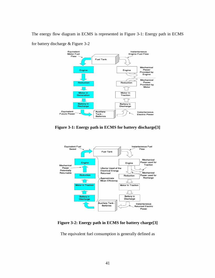
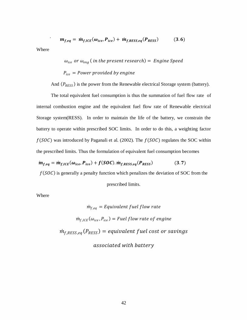
The energy flow diagram in ECMS is represented in Figure 3-1: Energy path in ECMS

for battery discharge & Figure 3-2

Figure 3-1: Energy path in ECMS for battery discharge[3]

Figure 3-2: Energy path in ECMS for battery charge[3]

The equivalent fuel consumption is generally defined as

42

𝒎 𝒇,𝒆𝒒 = 𝒎 𝒇,𝑰𝑪𝑬 𝝎𝒊𝒄𝒆,𝑷𝒊𝒄𝒆 + 𝒎 𝒇,𝑹𝑬𝑺𝑺,𝒆𝒒 𝑷𝑹𝑬𝑺𝑺 (𝟑.𝟔)

Where

𝜔𝑖𝑐𝑒 𝑜𝑟 𝜔𝑒𝑛𝑔 𝑖𝑛 𝑡𝑕𝑒 𝑝𝑟𝑒𝑠𝑒𝑛𝑡 𝑟𝑒𝑠𝑒𝑎𝑟𝑐𝑕 = 𝐸𝑛𝑔𝑖𝑛𝑒 𝑆𝑝𝑒𝑒𝑑

𝑃𝑖𝑐𝑒 = 𝑃𝑜𝑤𝑒𝑟 𝑝𝑟𝑜𝑣𝑖𝑑𝑒𝑑 𝑏𝑦 𝑒𝑛𝑔𝑖𝑛𝑒

And 𝑃𝑅𝐸𝑆𝑆 is the power from the Renewable electrical Storage system (battery).

The total equivalent fuel consumption is thus the summation of fuel flow rate of

internal combustion engine and the equivalent fuel flow rate of Renewable electrical

Storage system(RESS). In order to maintain the life of the battery, we constrain the

battery to operate within prescribed SOC limits. In order to do this, a weighting factor

𝑓(𝑆𝑂𝐶) was introduced by Paganali et al. (2002). The 𝑓(𝑆𝑂𝐶) regulates the SOC within

the prescribed limits. Thus the formulation of equivalent fuel consumption becomes

𝒎 𝒇,𝒆𝒒 = 𝒎 𝒇,𝑰𝑪𝑬 𝝎𝒊𝒄𝒆,𝑷𝒊𝒄𝒆 + 𝒇 𝑺𝑶𝑪 .𝒎 𝒇,𝑹𝑬𝑺𝑺,𝒆𝒒 𝑷𝑹𝑬𝑺𝑺 (𝟑.𝟕)

𝑓 𝑆𝑂𝐶 is generally a penalty function which penalizes the deviation of SOC from the

prescribed limits.

Where

𝑚 𝑓 ,𝑒𝑞 = 𝐸𝑞𝑢𝑖𝑣𝑎𝑙𝑒𝑛𝑡 𝑓𝑢𝑒𝑙 𝑓𝑙𝑜𝑤 𝑟𝑎𝑡𝑒

𝑚 𝑓 ,𝐼𝐶𝐸 𝜔𝑖𝑐𝑒 ,𝑃𝑖𝑐𝑒 = 𝐹𝑢𝑒𝑙 𝑓𝑙𝑜𝑤 𝑟𝑎𝑡𝑒 𝑜𝑓 𝑒𝑛𝑔𝑖𝑛𝑒

𝑚 𝑓,𝑅𝐸𝑆𝑆 ,𝑒𝑞 𝑃𝑅𝐸𝑆𝑆 = 𝑒𝑞𝑢𝑖𝑣𝑎𝑙𝑒𝑛𝑡 𝑓𝑢𝑒𝑙 𝑐𝑜𝑠𝑡 𝑜𝑟 𝑠𝑎𝑣𝑖𝑛𝑔𝑠

𝑎𝑠𝑠𝑜𝑐𝑖𝑎𝑡𝑒𝑑 𝑤𝑖𝑡𝑕 𝑏𝑎𝑡𝑡𝑒𝑟𝑦

43

CHAPTER FOUR: ECMS AND ITS IMPLEMENTATION

Formulation of equations in ECMS for a power split hybrid

In a power split hybrid 𝑃𝑒𝑙 can be divided into three cases

𝑷𝑹𝑬𝑺𝑺 =𝑷𝑴𝑮𝟐

𝜼𝑷𝑬 .𝜼𝒃,𝒅𝒊𝒔.𝜼𝑴𝑮𝟐− (𝑷𝑴𝑮𝟏.𝜼𝑷𝑬 .𝜼𝒃,𝒄𝒉𝒈.𝜼𝑴𝑮𝟏) (𝟒.𝟏)

𝑃𝑀𝐺1 > 0 (𝐺𝑒𝑛𝑒𝑟𝑎𝑡𝑜𝑟 𝑚𝑜𝑑𝑒) 𝑎𝑛𝑑 𝑃𝑀𝐺2 > 0(𝑀𝑜𝑡𝑜𝑟 𝑚𝑜𝑑𝑒)

𝑷𝑹𝑬𝑺𝑺 =𝑷𝑴𝑮𝟐

𝜼𝑷𝑬 .𝜼𝒃,𝒅𝒊𝒔.𝜼𝑴𝑮𝟐−

𝑷𝑴𝑮𝟏

𝜼𝑷𝑬 .𝜼𝒃,𝒅𝒊𝒔.𝜼𝑴𝑮𝟏 (𝟒.𝟐)

𝑃𝑀𝐺1 ≤ 0 𝑀𝑜𝑡𝑜𝑟 𝑚𝑜𝑑𝑒 𝑎𝑛𝑑 𝑃𝑀𝐺2 ≥ 0 (𝑀𝑜𝑡𝑜𝑟 𝑚𝑜𝑑𝑒)

𝑷𝑹𝑬𝑺𝑺 = 𝑷𝑴𝑮𝟐.𝜼𝑷𝑬 .𝜼𝒃,𝒄𝒉𝒈.𝜼𝑴𝑮𝟐 − 𝑷𝑴𝑮𝟏 .𝜼𝑷𝑬 .𝜼𝒃,𝒄𝒉𝒈.𝜼𝑴𝑮𝟏 (𝟒.𝟑)

𝑃𝑀𝐺2 ≤ 0 𝐺𝑒𝑛𝑒𝑟𝑎𝑡𝑜𝑟 𝑚𝑜𝑑𝑒 𝑃𝑀𝐺1 ≥ 0(𝐺𝑒𝑛𝑒𝑟𝑎𝑡𝑜𝑟 𝑚𝑜𝑑𝑒)

From the Basic equation of Instantaneous fuel consumption minimization one can write

the fuel minimization equation for a power split hybrid in the following way [3].

𝒎 𝒇,𝑹𝑬𝑺𝑺,𝒆𝒒(𝑷𝑹𝑬𝑺𝑺) =

𝟏

𝑸𝒍𝒉𝒗 . (𝑺𝒄𝒉𝒈.

(𝑷𝑴𝑮𝟐/𝜼𝑴𝑮𝟐) − (𝑷𝑴𝑮𝟏/𝜼𝑴𝑮𝟏)

𝜼𝑷𝑬 .𝜼𝒃,𝒅𝒊𝒔 .𝜸𝟏

+ 𝑺𝒅𝒊𝒔. 𝑷𝑴𝑮𝟐 .𝜼𝑴𝑮𝟐 −𝑷𝑴𝑮𝟏.𝜼𝑴𝑮𝟏 ∗ 𝜼𝑷𝑬 .𝜼𝒃,𝒄𝒉𝒈 . (𝟏 − 𝜸𝟏)).𝜸𝟐+ (𝑺𝒄𝒉𝒈.𝜸𝟑. (𝟏 + 𝒔𝒊𝒈𝒏(𝜸𝟑)))/𝟐 + 𝑺𝒅𝒊𝒔.𝜸𝟑. (𝟏 − 𝒔𝒊𝒈𝒏(𝜸𝟑))/𝟐). (𝟏

− 𝜸𝟐) (𝟒.𝟒)

𝛾1 =1+𝑠𝑖𝑔𝑛 𝑃𝑀𝐺 2

2

𝛾2 =1−𝑠𝑖𝑔𝑛 𝑃𝑀𝐺 2 .𝑃𝑀𝐺 1

2

𝛾3 =𝑃𝑀𝐺 2

𝜂𝑃𝐸 .𝜂𝑏 ,𝑑𝑖𝑠 .𝜂𝑀𝐺 2− 𝑃𝑀𝐺1 .𝜂𝑃𝐸 . 𝜂𝑏 ,𝑐𝑕𝑔 .𝜂𝑀𝐺1

44

Where

𝑃𝑀𝐺2 = 𝑃𝑜𝑤𝑒𝑟 𝑜𝑓 𝑀𝐺2 [𝑀𝑒𝑐𝑕𝑎𝑛𝑖𝑐𝑎𝑙]

𝑃𝑀𝐺1 = 𝑃𝑜𝑤𝑒𝑟 𝑜𝑓 (𝑀𝐺1)[𝑀𝑒𝑐𝑕𝑎𝑛𝑖𝑐𝑎𝑙]

𝑃𝑅𝐸𝑆𝑆 = 𝑃𝑜𝑤𝑒𝑟 𝑜𝑓 𝑅𝐸𝑆𝑆 𝑏𝑎𝑡𝑡𝑒𝑟𝑦 [𝐸𝑙𝑒𝑐𝑡𝑟𝑖𝑐𝑎𝑙]

𝜂𝑃𝐸 = 𝐸𝑓𝑓𝑖𝑐𝑖𝑒𝑛𝑐𝑦 𝑜𝑓 𝑃𝑜𝑤𝑒𝑟 𝐸𝑙𝑒𝑐𝑡𝑟𝑜𝑛𝑖𝑐𝑠

𝜂𝑏 ,𝑑𝑖𝑠 = 𝐸𝑓𝑓𝑖𝑐𝑖𝑒𝑛𝑐𝑦 𝑜𝑓 𝑏𝑎𝑡𝑡𝑒𝑟𝑦 𝑑𝑢𝑟𝑖𝑛𝑔 𝑑𝑖𝑠𝑐𝑕𝑎𝑟𝑔𝑒

𝜂𝑏 ,𝑐𝑕𝑔 = 𝐸𝑓𝑓𝑖𝑐𝑖𝑒𝑛𝑐𝑦 𝑜𝑓 𝑏𝑎𝑡𝑡𝑒𝑟𝑦 𝑑𝑢𝑟𝑖𝑛𝑔 𝑐𝑕𝑎𝑟𝑔𝑒

𝑄𝑙𝑕𝑣 = 𝐿𝑜𝑤𝑒𝑟 𝐻𝑒𝑎𝑡𝑖𝑛𝑔 𝑣𝑎𝑙𝑢𝑒 𝑜𝑓 𝑓𝑢𝑒𝑙

𝑆𝑐𝑕𝑔 = 1𝜂𝑐𝑕𝑔 ,𝑆𝑑𝑖𝑠 = 𝜂𝑑𝑖𝑠

𝜂𝑐𝑕𝑔 = 𝐴𝑣𝑒𝑟𝑎𝑔𝑒 𝑒𝑓𝑓𝑖𝑐𝑖𝑒𝑛𝑐𝑦 𝑖𝑛 𝑎𝑙𝑙 𝑐𝑕𝑎𝑟𝑔𝑖𝑛𝑔 𝑐𝑜𝑛𝑑𝑖𝑡𝑖𝑜𝑛𝑠

𝜂𝑑𝑖𝑠 = 𝐴𝑣𝑒𝑟𝑎𝑔𝑒 𝑒𝑓𝑓𝑖𝑐𝑖𝑒𝑛𝑐𝑦 𝑖𝑛 𝑎𝑙𝑙 𝑑𝑖𝑠𝑐𝑕𝑎𝑟𝑔𝑖𝑛𝑔 𝑐𝑜𝑛𝑑𝑖𝑡𝑖𝑜𝑛𝑠

The charge and discharge coefficients, 𝑆𝑐𝑕𝑔 𝑎𝑛𝑑 𝑆𝑑𝑖𝑠 , in practical situations are

considered as unknown parameters to be tuned. Although Dynamic Programming

requires you to know the whole driving cycle a priori, the validity of ECMS algorithm

depends on the tuning of parameters 𝑆𝑐𝑕𝑔 , 𝑆𝑑𝑖𝑠 . The parameters are very sensitive and

right tuning of these parameters would help one realize a charge sustaining behavior

In particular, using the battery to supply the power demand lowers the fuel

consumption, but an additional amount of energy is needed in future to recharge the

battery and similarly using engine to charge the battery increases the instantaneous fuel

consumption but this reduces the fuel consumption in future since the energy is saved for

future use. Hence the equivalent fuel consumption is regarded as the sum of

45

instantaneous fuel consumption of both engine and battery. The Control strategy has to

minimize the fuel consumption and at the same time meet the driver power request. To

meet the power request the controller has to know the power request and decide between

the power split between the various actuators that minimizes the instantaneous fuel

consumption. ECMS control strategy can be applied in real time unlike dynamic

programming which is computationally extensive and at the same time requires the

driving cycle be known a priori. In the present research, the implementation of ECMS

strategy in both forward and backward models is the same except for the dynamics

involved in the forward model.

In this section we will go step by step through the higher level supervisory

controller and how the controller responds to the control signals and how it optimizes the

fuel consumption. The model dynamics are modeled in MATLAB/Simulink and an

embedded s-function is called each time to calculate the optimal fuel consumption of the

model. A plug-in hybrid electric vehicle operates in two modes.

Charge Depletion mode

Charge Sustaining mode

In charge depletion mode, the vehicle has the capacity to use its off-board energy

and run the vehicle in almost pure electric mode. The engine turns on only when the

power demand crosses a particular threshold. Charge sustaining mode is activated when

the state of charge falls below a particular threshold and in this mode optimization based

on ECMS is implemented. The difference in calculation of fuel consumption in both is

based on the fact that in charge depletion mode a direct conversion factor of electrical

energy to fuel is considered depending on the cost of electricity and fuel and in charge

46

sustaining mode this is carried out by assigning future costs and future savings to the

present usage of electrical energy.

The supervisory controller acts in two modes in the following way.

Implementation inside the supervisory control is by far the same in a forward modeling

approach and backward modeling approach except for a the dynamics that has been

neglected in the backward model.

4.1 Implementation inside the supervisory controller

START

INPUT

SOC

SOC>0.5

CHARGE

SUSTAINING(ECMS)

CHARGE

DEPLETING

NO YES

Figure 4-1: Controller Chekcing for SOC limits

47

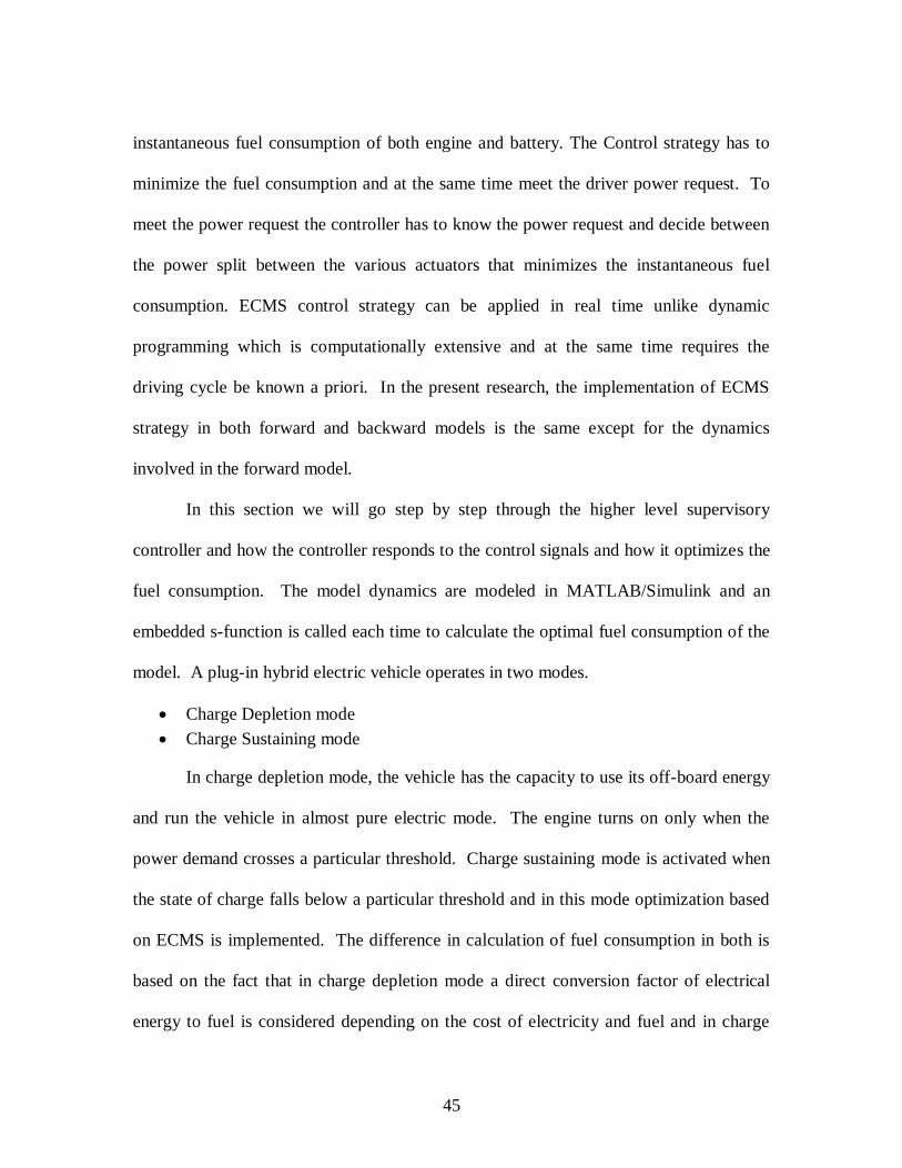
4.1.1 Implementation in Charge Depletion mode

Figure 4-2: Engine On/Off Strategy

The Figure 4-1 shows the schematic representation of controller switching between

charge Depletion mode and ECMS. And similarly the Figure 4-2 shows the engine

turning on and off when the power request is more than the power provided by the motor

coupled directly to the ring gear. When the engine is ON which is shown in the Figure

4-3: Algorithm for power flow in charge depletion mode, the controller decides to turn

the engine OFF or keep it ON depending on the power-request and the ENGINE ON/OFF

time which is calculated inside the supervisory controller based on the engine current

speed and optimal speed of the engine.

Here 𝑆𝑂𝐶𝑚𝑎𝑥 = 𝑆𝑡𝑎𝑡𝑒 𝑜𝑓 𝑐𝑕𝑎𝑟𝑔𝑒 𝑓𝑜𝑟 𝑡𝑕𝑒 𝐸𝐶𝑀𝑆 𝑜𝑝𝑒𝑟𝑎𝑡𝑖𝑜𝑛 𝑡𝑜 𝑡𝑟𝑖𝑔𝑔𝑒𝑟

In this research we choose it to be 0.5.

𝑆𝑂𝐶𝑚𝑎𝑥 = 0.5

𝑆𝑂𝐶 < 𝑆𝑂𝐶𝑚𝑎𝑥

𝑝𝑤𝑟𝑟𝑒𝑞 ≥ 𝑝𝑤𝑟𝑀𝐺2−𝑚𝑎𝑥

𝜔𝑒𝑛𝑔 < 𝜔𝑖𝑑𝑙𝑒

START ENGINE

AND

YES YES

48

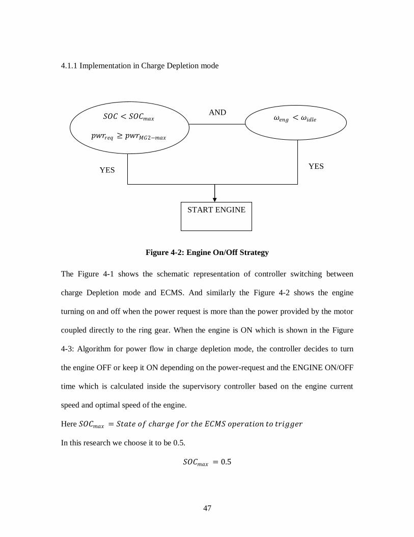
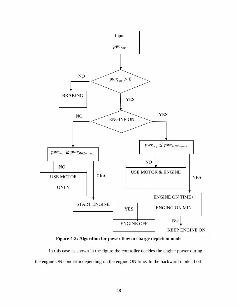
Figure 4-3: Algorithm for power flow in charge depletion mode

In this case as shown in the figure the controller decides the engine power during

the engine ON condition depending on the engine ON time. In the backward model, both

𝑝𝑤𝑟𝑟𝑒𝑞

Input

𝑝𝑤𝑟𝑟𝑒𝑞 > 0

BRAKING

NO

YES

ENGINE ON

𝑝𝑤𝑟𝑟𝑒𝑞 ≥ 𝑝𝑤𝑟𝑀𝐺2−𝑚𝑎𝑥

𝑝𝑤𝑟𝑟𝑒𝑞 ≤ 𝑝𝑤𝑟𝑀𝐺2−𝑚𝑎𝑥

NO

YES

START ENGINE

USE MOTOR

ONLY

NO YES

USE MOTOR & ENGINE

ENGINE ON TIME>

ENGING ON MIN

NO

YES

ENGINE OFF

KEEP ENGINE ON

YES

NO

49

the speed and power are decided inside the supervisory controller, but in the forward

model speed is the outcome of power based on the equation () that is calculated outside

the supervisory controller in the engine dynamics block. This speed is the integral of the

torque and this speed is saturated between the limits idle speed and maximum engine

speed. The engine speed becomes zero when the engine is on for more than the engine

ON minimum time and when the engine power becomes zero. The only difference in

both the modeling approaches lies in the fact that the engine speed and engine power are

dictated by the supervisory controller in backward model, but in forward model the speed

is derived from the dynamic power balance equation as an outcome of power.

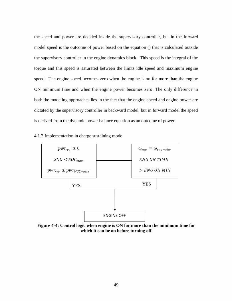
4.1.2 Implementation in charge sustaining mode

Figure 4-4: Control logic when engine is ON for more than the minimum time for

which it can be on before turning off

𝑝𝑤𝑟𝑟𝑒𝑞 ≥ 0

𝑆𝑂𝐶 < 𝑆𝑂𝐶𝑚𝑎𝑥

𝑝𝑤𝑟𝑟𝑒𝑞 ≤ 𝑝𝑤𝑟𝑀𝐺2−𝑚𝑎𝑥

𝜔𝑒𝑛𝑔 = 𝜔𝑒𝑛𝑔 −𝑖𝑑𝑙𝑒

𝐸𝑁𝐺 𝑂𝑁 𝑇𝐼𝑀𝐸

> 𝐸𝑁𝐺 𝑂𝑁 𝑀𝐼𝑁

ENGINE OFF

YES YES

50

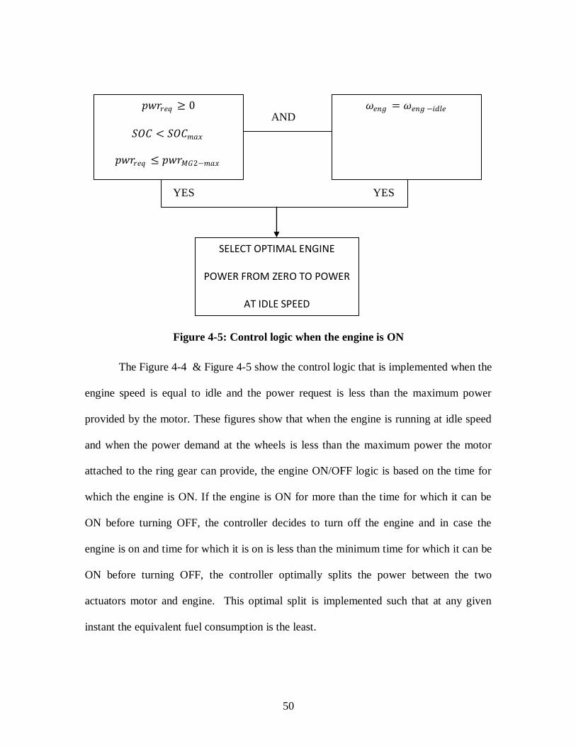
Figure 4-5: Control logic when the engine is ON

The Figure 4-4 & Figure 4-5 show the control logic that is implemented when the

engine speed is equal to idle and the power request is less than the maximum power

provided by the motor. These figures show that when the engine is running at idle speed

and when the power demand at the wheels is less than the maximum power the motor

attached to the ring gear can provide, the engine ON/OFF logic is based on the time for

which the engine is ON. If the engine is ON for more than the time for which it can be

ON before turning OFF, the controller decides to turn off the engine and in case the

engine is on and time for which it is on is less than the minimum time for which it can be

ON before turning OFF, the controller optimally splits the power between the two

actuators motor and engine. This optimal split is implemented such that at any given

instant the equivalent fuel consumption is the least.

AND

YES YES

𝑝𝑤𝑟𝑟𝑒𝑞 ≥ 0

𝑆𝑂𝐶 < 𝑆𝑂𝐶𝑚𝑎𝑥

𝑝𝑤𝑟𝑟𝑒𝑞 ≤ 𝑝𝑤𝑟𝑀𝐺2−𝑚𝑎𝑥

𝜔𝑒𝑛𝑔 = 𝜔𝑒𝑛𝑔 −𝑖𝑑𝑙𝑒

SELECT OPTIMAL ENGINE

POWER FROM ZERO TO POWER

AT IDLE SPEED

51

𝑆𝑂𝐶 < 𝑆𝑂𝐶𝑚𝑎𝑥

𝑝𝑤𝑟𝑟𝑒𝑞 ≥ 0

𝜔𝑒𝑛𝑔 < 𝜔𝑒𝑛𝑔 −𝑖𝑑𝑙𝑒

𝑝𝑤𝑟𝑀𝐺2 ≥ 0

𝑝𝑤𝑟𝑀𝐺2 ≤ 𝑝𝑤𝑟𝑀𝐺2−𝑚𝑎𝑥

𝑝𝑤𝑟𝑀𝐺2 ≤ 𝑝𝑤𝑟𝑟𝑒𝑞

𝑝𝑤𝑟𝑀𝐺2 ≥ 0

𝑝𝑤𝑟𝑀𝐺2 ≥ 𝑝𝑤𝑟𝑀𝐺2−𝑚𝑎𝑥

𝑝𝑤𝑟𝑀𝐺2 ≤ 𝑝𝑤𝑟𝑟𝑒𝑞

START

ENGINE

Test Cost of Starting <=

Cost of Non-starting

START ENGINE

Figure 4-6: Control logic when engine speed is less than idle speed

52

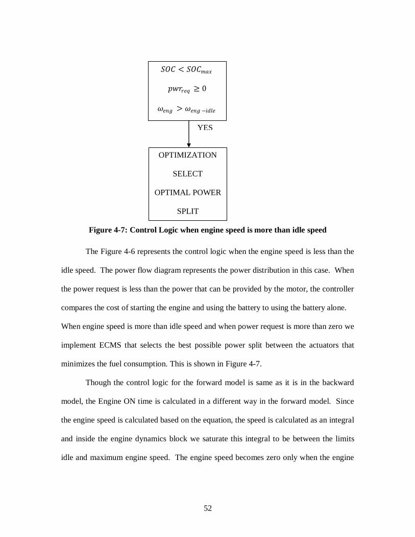
Figure 4-7: Control Logic when engine speed is more than idle speed

The Figure 4-6 represents the control logic when the engine speed is less than the

idle speed. The power flow diagram represents the power distribution in this case. When

the power request is less than the power that can be provided by the motor, the controller

compares the cost of starting the engine and using the battery to using the battery alone.

When engine speed is more than idle speed and when power request is more than zero we

implement ECMS that selects the best possible power split between the actuators that

minimizes the fuel consumption. This is shown in Figure 4-7.

Though the control logic for the forward model is same as it is in the backward

model, the Engine ON time is calculated in a different way in the forward model. Since

the engine speed is calculated based on the equation, the speed is calculated as an integral

and inside the engine dynamics block we saturate this integral to be between the limits

idle and maximum engine speed. The engine speed becomes zero only when the engine

YES

𝑆𝑂𝐶 < 𝑆𝑂𝐶𝑚𝑎𝑥

𝑝𝑤𝑟𝑟𝑒𝑞 ≥ 0

𝜔𝑒𝑛𝑔 > 𝜔𝑒𝑛𝑔 −𝑖𝑑𝑙𝑒

OPTIMIZATION

SELECT

OPTIMAL POWER

SPLIT

53

is on for more than the time specified by the Engine minimum on time and the power

delivered by the engine (coming as an output from supervisory controller) becomes zero

Since the integral saturates the engine speed outside the supervisory controller and in the

engine dynamics subsystem, it is slightly different from the backward model far as the

implementation is concerned in MATLAB/Simulink, but the inherent logic is the same.

4.2 Differences in Practical implementation between Forward modeling approach and

backward modeling approach

In this present research we have modeled a power-split plug-in hybrid electric

vehicle by using two approaches. The first one was backward modeling approach and the

second is slightly different form of modeling which removes any assumptions we

considered in backward approach. The backward model was more of a simplistic model

as it moves forward by assuming that the power at the wheels is distributed and is always

met. This cannot be applied in modeling real time systems as the real power-train has to

have a driver block which computes the power demand which is different from the one

computed in the backward model. The supervisory controller on the other hand in the

backward model assumes certain dynamics without having any real time blocks. It

computes the output and the controller decides the speed of the individual actuators based

on the control inputs and the states and this eliminates the use of any individual

subsystems. The individual subsystems are used only to check for the efficiency losses.

The supervisory controller in the forward model does not have any control on the speed.

It computes the control inputs to suit the power demand and based on the outputs

54

provided by the higher level controller the real speed of the actuators is computed. The

power provided by the supervisory controller is given as an input to the individual

systems to check for the limitations. The forward model proceeds from the driver through

the power-train to the wheels. This is schematically represented in

Component Sizing for the power-train in the dissertation

The power-train components and sizing used in the dissertation is the THS-II

configuration released by Toyota corporation in the year 2004[22]. The 2004 Production

Prius is limited to charge sustaining operation only[22]. The Hymotion PHEV

introduced by Toyota had an additional battery pack to have the charge depletion

operation accomplished. The Production Prius had a 6Ah, 1.3kWh, with charge

sustaining operation. The Hymotion Prius which is a PHEV had an additional 5kWh

battery pack. This combined battery pack weighed 73 kg when compared to the 44kg

battery pack of the production Prius. The Hymotion Prius used a lithium ion battery pack

which reduces the weight considerably and provides the same capacity for a lesser

weight. Thus the capacity to weight ratio is much better for the lithium ion battery pack,

which provides thrice the capacity for the same weight when compared to Nickel Metal

Hydride battery. In the present configuration used in the dissertation we use the THS-II

component sizing with the battery capacity increased to thrice since this configuration

uses Lithium Ion battery pack[22].

4.3 Simulation results

Hitherto mentioned ECMS(instantaneous minimization strategy) has been applied

for the two approaches i.e. backward and forward and the results are tabulated. The

55

simulator is a plug-in hybrid electric vehicle and hence the ECMS strategy is applied

after the state of charge of the battery reaches the threshold mentioned in the supervisory

controller. Hence the applied ECMS strategy helps one realize a charge sustaining

pattern. The charging and discharging parameters(𝑆𝑐𝑕𝑔 ,𝑆𝑑𝑖𝑠 ) are cycle dependent and

tuned to get the minimal fuel consumption and also charge sustaining pattern. The fuel

economy results and the system performance curves are tabulated for a backward model

and forward model. We tabulate the results for two cycles, the city cycle(FUDS or

UDDS) and the Federal Highway driving schedule.

In order to apply ECMS and comply with the strategy that has been formulated,

one needs to start in the charge sustaining pattern. The charge depleting pattern does not

involve any optimization and hence the vehicle is operated mostly in electric mode and

the equivalent cost of electricity in terms of fuel is presented.

4.3.1 Fuel economy for UDDS/FUDS cycle and FHDS cycle for charge sustaining

strategy

In this test, the simulation results for the simulation of the city cycle are

presented(FUDS) and highway cycle(FHDS) are presented The Cycle essentially is of

duration 1369 seconds and the cycle is repeated five times to see for the charge sustaining

pattern. FHDS cycle is of duration 770 seconds and the cycle is repeated five times. The

SOC of the battery starts at 0.5 and with the tuned parameters for that cycle it is well

maintained between 0.5 and 0.4.

56

Driving Cycle 𝑆𝑐𝑕𝑔 Mileage(MPG)

Equivalent fuel consumption

UDDS 2.4 56.55

FHDS 3.5 71.44

Table 4-1: Fuel consumption results for backward Model

Driving Cycle 𝑆𝑐𝑕𝑔 Mileage(MPG)

UDDS 2.2 56.87

FHDS 2.6 63.02

Table 4-2: Fuel consumption results for Forward Model

The fuel consumption results show the fuel economy for two cycles i.e. city cycle

and highway cycle. The optimal values for the coefficients were found by running the

cycle over a range of values chosen in order to select the ones that produce the minimum

fuel consumption for each cycle. The values for found by discritizing the charging and

discharging coefficients and running the simulations over a grid of chosen values. This

gives us the value for which fuel consumption is minimum.

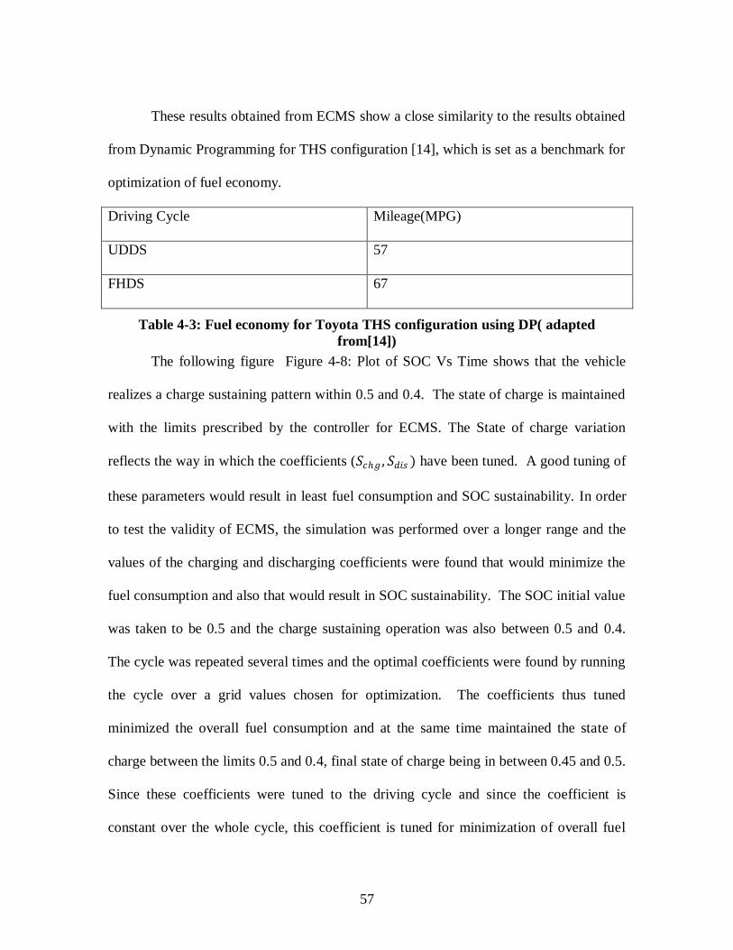
57

These results obtained from ECMS show a close similarity to the results obtained

from Dynamic Programming for THS configuration [14], which is set as a benchmark for

optimization of fuel economy.

Driving Cycle Mileage(MPG)

UDDS 57

FHDS 67

Table 4-3: Fuel economy for Toyota THS configuration using DP( adapted

from[14])

The following figure Figure 4-8: Plot of SOC Vs Time shows that the vehicle

realizes a charge sustaining pattern within 0.5 and 0.4. The state of charge is maintained

with the limits prescribed by the controller for ECMS. The State of charge variation

reflects the way in which the coefficients (𝑆𝑐𝑕𝑔 , 𝑆𝑑𝑖𝑠 ) have been tuned. A good tuning of

these parameters would result in least fuel consumption and SOC sustainability. In order

to test the validity of ECMS, the simulation was performed over a longer range and the

values of the charging and discharging coefficients were found that would minimize the

fuel consumption and also that would result in SOC sustainability. The SOC initial value

was taken to be 0.5 and the charge sustaining operation was also between 0.5 and 0.4.

The cycle was repeated several times and the optimal coefficients were found by running

the cycle over a grid values chosen for optimization. The coefficients thus tuned

minimized the overall fuel consumption and at the same time maintained the state of

charge between the limits 0.5 and 0.4, final state of charge being in between 0.45 and 0.5.

Since these coefficients were tuned to the driving cycle and since the coefficient is

constant over the whole cycle, this coefficient is tuned for minimization of overall fuel

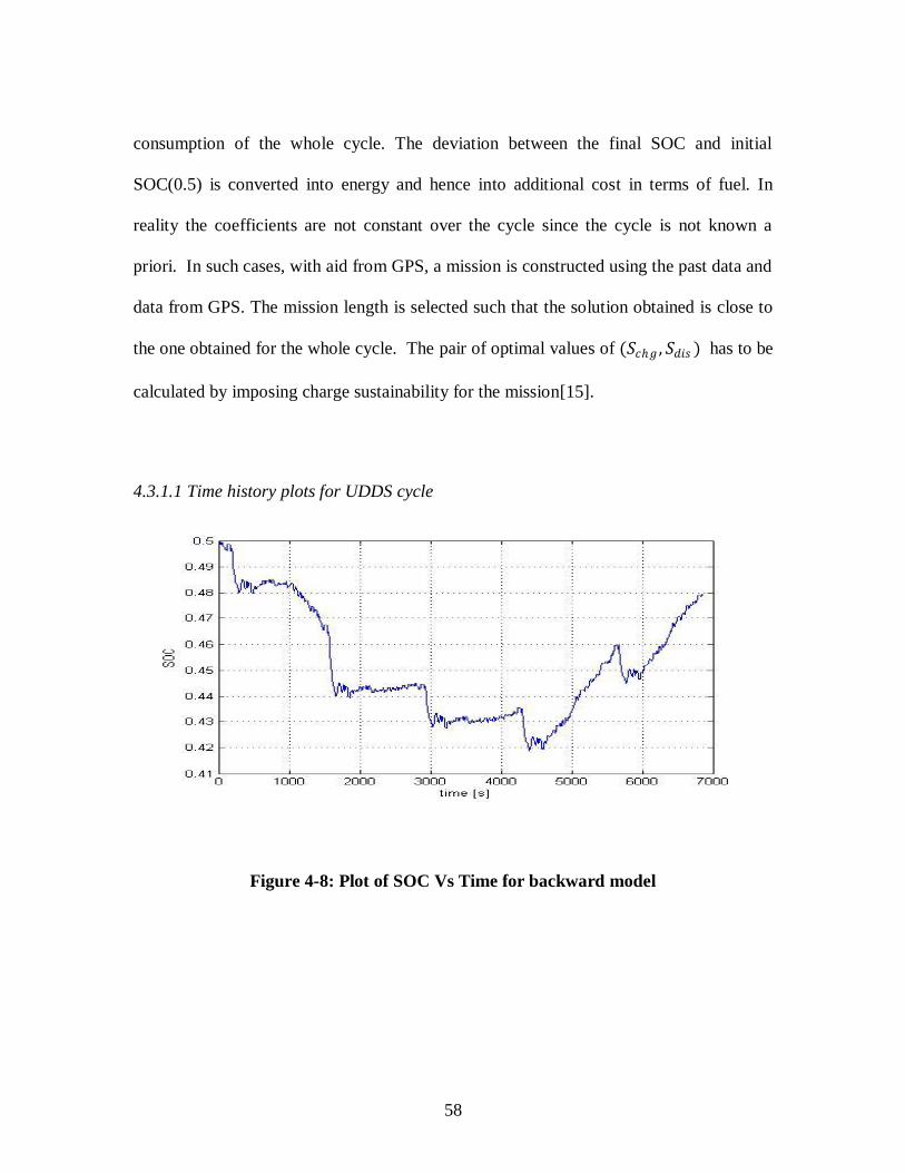
58

consumption of the whole cycle. The deviation between the final SOC and initial

SOC(0.5) is converted into energy and hence into additional cost in terms of fuel. In

reality the coefficients are not constant over the cycle since the cycle is not known a

priori. In such cases, with aid from GPS, a mission is constructed using the past data and

data from GPS. The mission length is selected such that the solution obtained is close to

the one obtained for the whole cycle. The pair of optimal values of (𝑆𝑐𝑕𝑔 , 𝑆𝑑𝑖𝑠 ) has to be

calculated by imposing charge sustainability for the mission[15].

4.3.1.1 Time history plots for UDDS cycle

Figure 4-8: Plot of SOC Vs Time for backward model

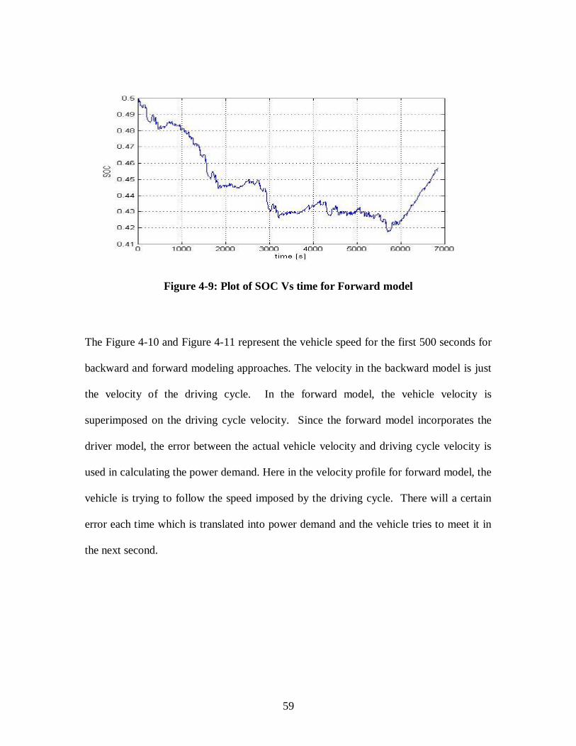
59

Figure 4-9: Plot of SOC Vs time for Forward model

The Figure 4-10 and Figure 4-11 represent the vehicle speed for the first 500 seconds for

backward and forward modeling approaches. The velocity in the backward model is just

the velocity of the driving cycle. In the forward model, the vehicle velocity is

superimposed on the driving cycle velocity. Since the forward model incorporates the

driver model, the error between the actual vehicle velocity and driving cycle velocity is

used in calculating the power demand. Here in the velocity profile for forward model, the

vehicle is trying to follow the speed imposed by the driving cycle. There will a certain

error each time which is translated into power demand and the vehicle tries to meet it in

the next second.

60

Figure 4-10: Velocity profile for backward model

Figure 4-11: velocity profile for forward model

61

Figure 4-12: Optimal Engine Power for backward model

Figure 4-13: Optimal engine power for forward model

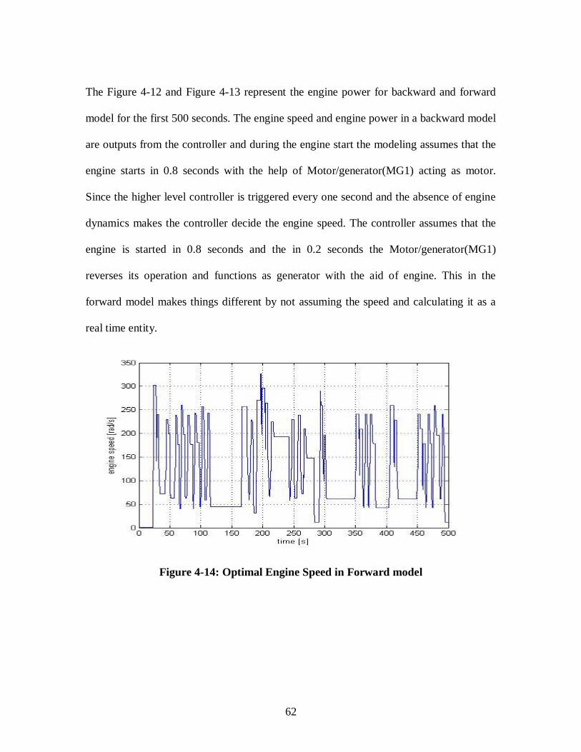
62

The Figure 4-12 and Figure 4-13 represent the engine power for backward and forward

model for the first 500 seconds. The engine speed and engine power in a backward model

are outputs from the controller and during the engine start the modeling assumes that the

engine starts in 0.8 seconds with the help of Motor/generator(MG1) acting as motor.

Since the higher level controller is triggered every one second and the absence of engine

dynamics makes the controller decide the engine speed. The controller assumes that the

engine is started in 0.8 seconds and the in 0.2 seconds the Motor/generator(MG1)

reverses its operation and functions as generator with the aid of engine. This in the

forward model makes things different by not assuming the speed and calculating it as a

real time entity.

Figure 4-14: Optimal Engine Speed in Forward model

63

Figure 4-15: Optimal Engine speed for backward model

The Figure 4-14 and Figure 4-15 represent the time history plots of engine speed in

forward and backward models.

Figure 4-16: Power curves for Forward model

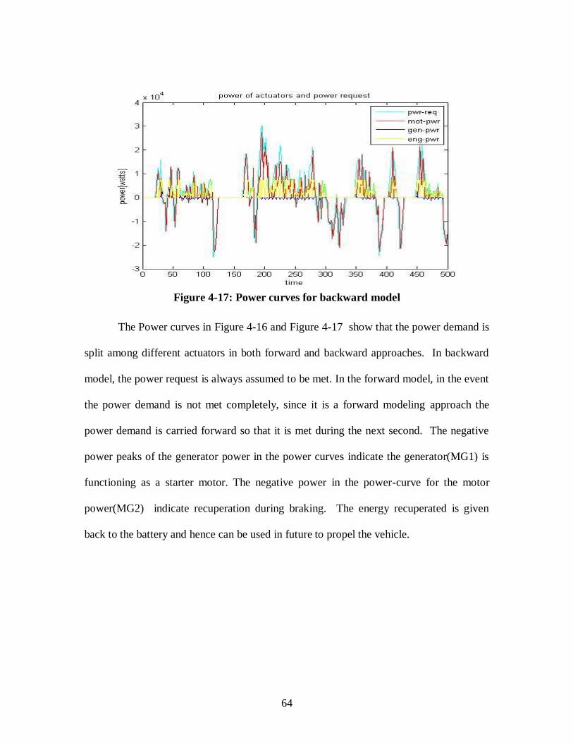
64

Figure 4-17: Power curves for backward model

The Power curves in Figure 4-16 and Figure 4-17 show that the power demand is

split among different actuators in both forward and backward approaches. In backward

model, the power request is always assumed to be met. In the forward model, in the event

the power demand is not met completely, since it is a forward modeling approach the

power demand is carried forward so that it is met during the next second. The negative

power peaks of the generator power in the power curves indicate the generator(MG1) is

functioning as a starter motor. The negative power in the power-curve for the motor

power(MG2) indicate recuperation during braking. The energy recuperated is given

back to the battery and hence can be used in future to propel the vehicle.

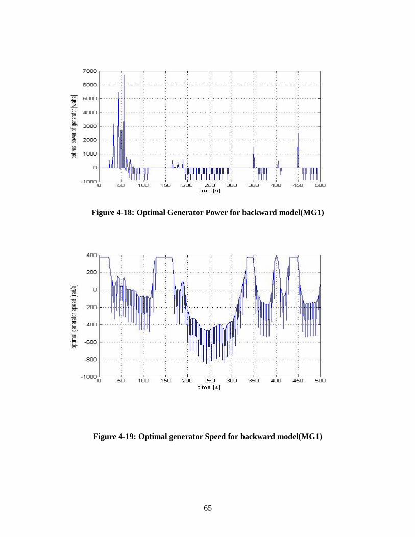
65

Figure 4-18: Optimal Generator Power for backward model(MG1)

Figure 4-19: Optimal generator Speed for backward model(MG1)

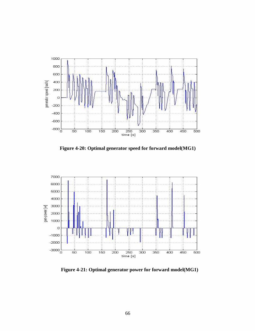
66

Figure 4-20: Optimal generator speed for forward model(MG1)

Figure 4-21: Optimal generator power for forward model(MG1)

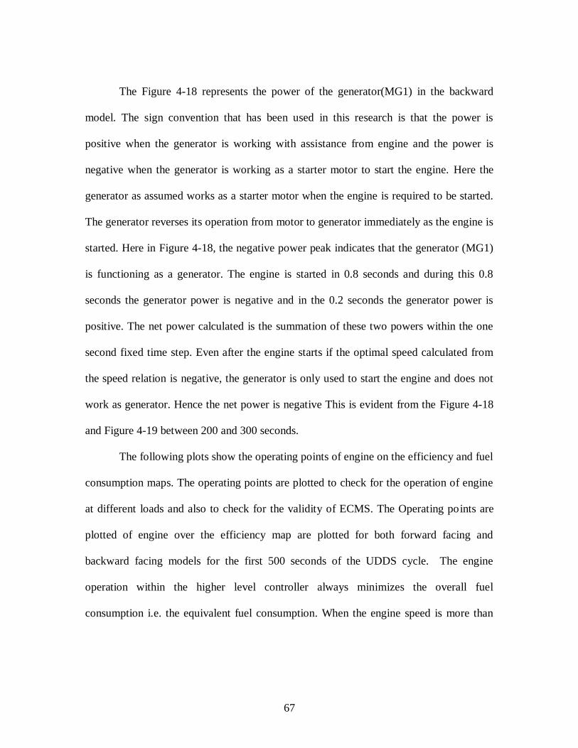
67

The Figure 4-18 represents the power of the generator(MG1) in the backward

model. The sign convention that has been used in this research is that the power is

positive when the generator is working with assistance from engine and the power is

negative when the generator is working as a starter motor to start the engine. Here the

generator as assumed works as a starter motor when the engine is required to be started.

The generator reverses its operation from motor to generator immediately as the engine is

started. Here in Figure 4-18, the negative power peak indicates that the generator (MG1)

is functioning as a generator. The engine is started in 0.8 seconds and during this 0.8

seconds the generator power is negative and in the 0.2 seconds the generator power is

positive. The net power calculated is the summation of these two powers within the one

second fixed time step. Even after the engine starts if the optimal speed calculated from

the speed relation is negative, the generator is only used to start the engine and does not

work as generator. Hence the net power is negative This is evident from the Figure 4-18

and Figure 4-19 between 200 and 300 seconds.

The following plots show the operating points of engine on the efficiency and fuel

consumption maps. The operating points are plotted to check for the operation of engine

at different loads and also to check for the validity of ECMS. The Operating points are

plotted of engine over the efficiency map are plotted for both forward facing and

backward facing models for the first 500 seconds of the UDDS cycle. The engine

operation within the higher level controller always minimizes the overall fuel

consumption i.e. the equivalent fuel consumption. When the engine speed is more than

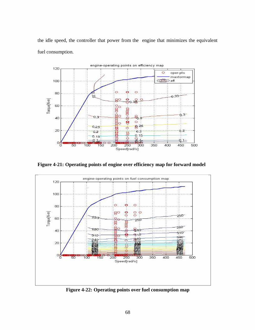
68

the idle speed, the controller that power from the engine that minimizes the equivalent

fuel consumption.

Figure 4-21: Operating points of engine over efficiency map for forward model

Figure 4-22: Operating points over fuel consumption map

69

The penalty function embedded within the equivalent fuel consumption always maintains

the charge within the region prescribed for charge sustenance. In this way, when the

engine speed is more than the idle speed, the controller minimizes the fuel consumption

and hence splits the power optimally between the actuators. If the engine speed is equal

to idle speed, depending on the engine ON/OFF time and also depending on the power

request, the engine power is chosen from zero to the power at idle speed. This

optimization picks up the power that minimizes the overall equivalent fuel consumption.

One can see from the plots that the engine operating at highest efficiency points has

comparatively lesser fuel consumption than the ones at lower efficiency.

Figure 4-23: Engine Torque associated with best efficiency

The Figure 4-23 shows the engine torque associated with best efficiency. The torque or

power that corresponds to the best efficiency line is selected for different speeds and this

is used during the optimization process. The engine speed is discritized and the

70

corresponding control variable is selected that satisfies the objective of minimizing the

fuel consumption. This control variable always corresponds to the best efficiency line.

The algorithm for the same power demand selects the points which gives the overall

minimum fuel consumption.

4.3.2 Calculation of fuel consumption in Charge Depletion Mode

Although the charge depletion mode in a plug-in hybrid electric vehicle is mostly electric,

the engine is turned on and off during high power demands. This makes it necessary to

calculate the costs associated with this fuel usage and also the range in pure electric

operation. We follow the calculation prescribed in[22] to calculate the mileage and also

the miles driven in electric mode. Here we use the term Petroleum displacement factor, to

determine how aggressively petroleum is used in charge depletion mode when compared

to charge sustaining operation[22].

𝑷𝒆𝒕𝒓𝒐𝒍𝒆𝒖𝒎 𝑫𝒊𝒔𝒑𝒍𝒂𝒄𝒆𝒎𝒆𝒏𝒕 𝑭𝒂𝒄𝒕𝒐𝒓(Adapted from [22])

= 𝟏 −

𝟏𝑴𝑷𝑮𝑪𝑫

𝟏

𝑴𝑷𝑮𝑪𝑺 ( 𝟒.𝟓)

This petroleum displacement factor is in turn used to calculate the range the vehicle can

drive if the vehicle were to operate in purely electric mode. This is defined as

𝑃𝐻𝐸𝑉 𝑒𝑞𝑢𝑖𝑣𝑎𝑙𝑒𝑛𝑡(Adapted from [22])

= 𝟏 −

𝟏𝑴𝑷𝑮𝑪𝑫

𝟏

𝑴𝑷𝑮𝑪𝑺 ∗ 𝑴𝒊𝒍𝒆𝒔𝑪𝑫 (𝟒.𝟔)

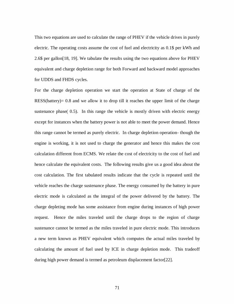
71

This two equations are used to calculate the range of PHEV if the vehicle drives in purely

electric. The operating costs assume the cost of fuel and electricity as 0.1$ per kWh and

2.6$ per gallon[18, 19]. We tabulate the results using the two equations above for PHEV

equivalent and charge depletion range for both Forward and backward model approaches

for UDDS and FHDS cycles.

For the charge depletion operation we start the operation at State of charge of the

RESS(battery)= 0.8 and we allow it to drop till it reaches the upper limit of the charge

sustenance phase( 0.5). In this range the vehicle is mostly driven with electric energy

except for instances when the battery power is not able to meet the power demand. Hence

this range cannot be termed as purely electric. In charge depletion operation- though the

engine is working, it is not used to charge the generator and hence this makes the cost

calculation different from ECMS. We relate the cost of electricity to the cost of fuel and

hence calculate the equivalent costs. The following results give us a good idea about the

cost calculation. The first tabulated results indicate that the cycle is repeated until the

vehicle reaches the charge sustenance phase. The energy consumed by the battery in pure

electric mode is calculated as the integral of the power delivered by the battery. The

charge depleting mode has some assistance from engine during instances of high power

request. Hence the miles traveled until the charge drops to the region of charge

sustenance cannot be termed as the miles traveled in pure electric mode. This introduces

a new term known as PHEV equivalent which computes the actual miles traveled by

calculating the amount of fuel used by ICE in charge depletion mode. This tradeoff

during high power demand is termed as petroleum displacement factor[22].

72

UDDS 1st cycle 2

nd cycle 3

rd cycle 4

th cycle

Fuel used[gal] 0.00073 0 0 0

Electricity

used[kWh]

0.78 0.79 0.79 .7056

Cost of fuel[$] .0019 0 0 0

Cost of

electricity[$]

0.078 0.079 0.079 0.07

Miles Driven 7.4 7.4 7.4 6.4

Table 4-4: Results for Charge depletion mode for UDDS cycle for backward model

The fourth UDDS cycle here is not purely charge depletion since it reaches the charge

sustenance phase before the cycle gets completed. Hence we take into consideration only

that phase till it reaches charge sustenance operation. The next table shows the results

tabulated for the UDDS cycle. The PHEV equivalent is calculated using the equation

The cost of electricity and cost of fuel used is tabulated. The 𝑀𝑃𝐺𝐶𝐷 term used in the

equation represents the miles per gallon in the Charge depletion mode. This is calculated

based on the amount of petroleum used in the charge depletion mode and the total miles

traveled in charge depletion mode.

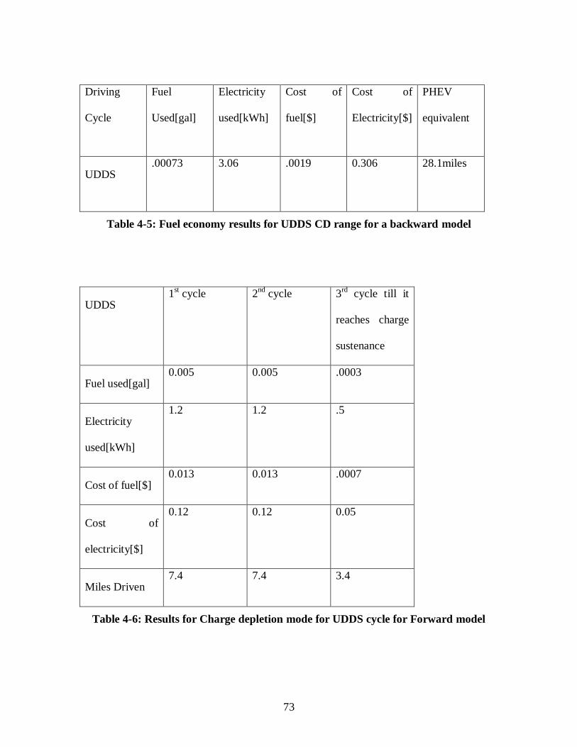
73

Driving

Cycle

Fuel

Used[gal]

Electricity

used[kWh]

Cost of

fuel[$]

Cost of

Electricity[$]

PHEV

equivalent

UDDS .00073 3.06 .0019 0.306 28.1miles

Table 4-5: Fuel economy results for UDDS CD range for a backward model

UDDS 1

st cycle 2

nd cycle 3

rd cycle till it

reaches charge

sustenance

Fuel used[gal] 0.005 0.005 .0003

Electricity

used[kWh]

1.2 1.2 .5

Cost of fuel[$] 0.013 0.013 .0007

Cost of

electricity[$]

0.12 0.12 0.05

Miles Driven 7.4 7.4 3.4

Table 4-6: Results for Charge depletion mode for UDDS cycle for Forward model

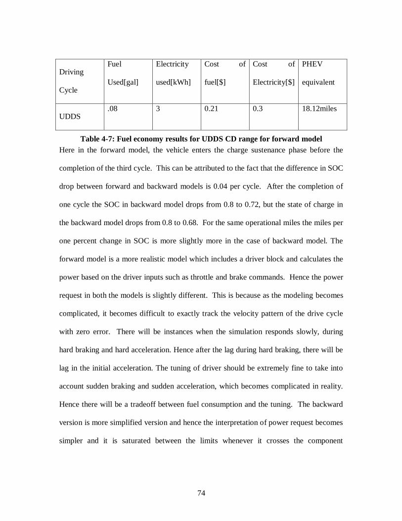
74

Driving

Cycle

Fuel

Used[gal]

Electricity

used[kWh]

Cost of

fuel[$]

Cost of

Electricity[$]

PHEV

equivalent

UDDS .08 3 0.21 0.3 18.12miles

Table 4-7: Fuel economy results for UDDS CD range for forward model

Here in the forward model, the vehicle enters the charge sustenance phase before the

completion of the third cycle. This can be attributed to the fact that the difference in SOC

drop between forward and backward models is 0.04 per cycle. After the completion of

one cycle the SOC in backward model drops from 0.8 to 0.72, but the state of charge in

the backward model drops from 0.8 to 0.68. For the same operational miles the miles per

one percent change in SOC is more slightly more in the case of backward model. The

forward model is a more realistic model which includes a driver block and calculates the

power based on the driver inputs such as throttle and brake commands. Hence the power

request in both the models is slightly different. This is because as the modeling becomes

complicated, it becomes difficult to exactly track the velocity pattern of the drive cycle

with zero error. There will be instances when the simulation responds slowly, during

hard braking and hard acceleration. Hence after the lag during hard braking, there will be

lag in the initial acceleration. The tuning of driver should be extremely fine to take into

account sudden braking and sudden acceleration, which becomes complicated in reality.

Hence there will be a tradeoff between fuel consumption and the tuning. The backward

version is more simplified version and hence the interpretation of power request becomes

simpler and it is saturated between the limits whenever it crosses the component

75

limitations. The forward model is just driver based and at each instant the power request

depends on the throttle and brake commands given by the driver. This can cause a slight

difference between the models and the mileage differs slightly.

Driving Cycle miles per one percent

change in SOC for

Backward model

miles per one percent

change in SOC for

Backward model

UDDS 0.92 0.61

Table 4-8: Miles per percent change in SOC for UDDS cycle

FHDS 1

st cycle 2

nd cycle 3

rd cycle till charge sustenance

Fuel used[gal] 0 0 .05

Electricity

used[kWh]

1.31 1.31 0.8

Cost of fuel[$] 0 0 0

Cost of

electricity[$]

.131 .131 0.08

Miles Driven 10.3 10.3 4.4

Table 4-9: Results for Charge depletion mode for FHDS cycle for backward model

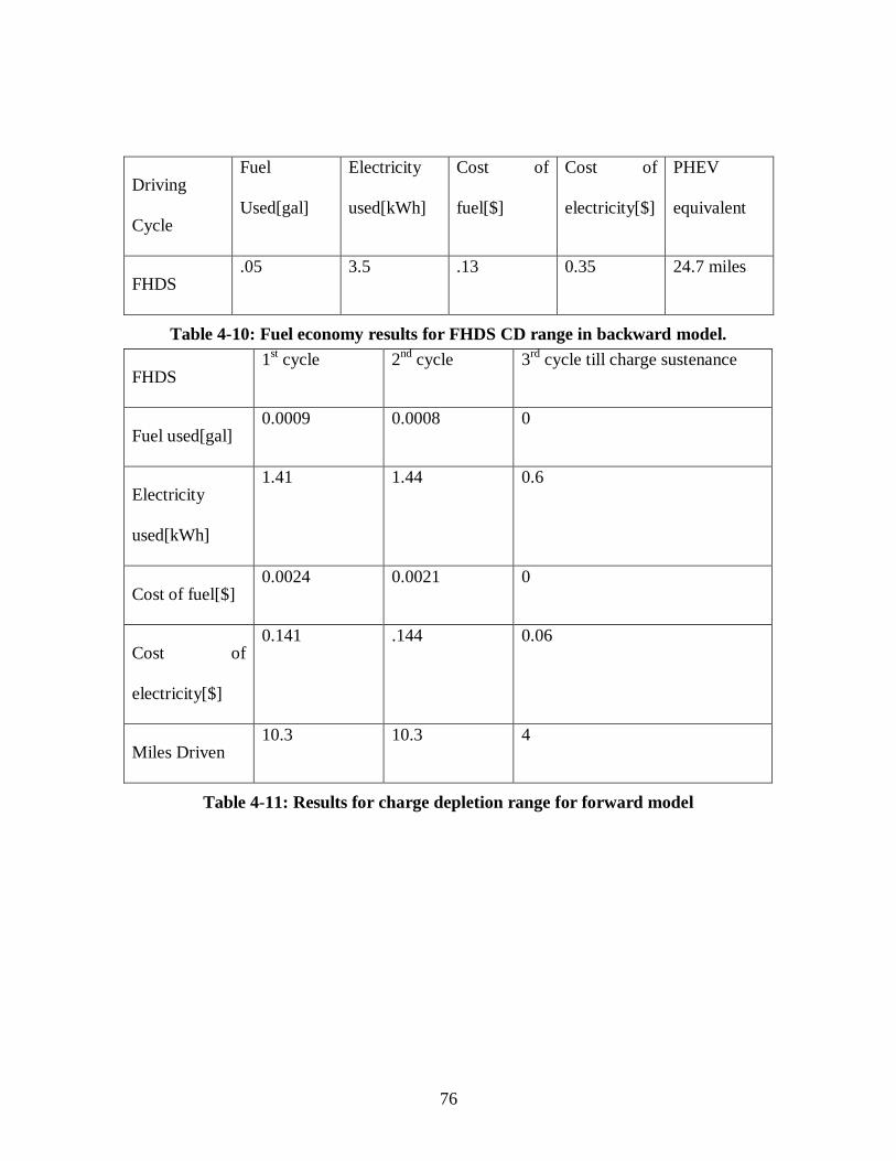
76

Driving

Cycle

Fuel

Used[gal]

Electricity

used[kWh]

Cost of

fuel[$]

Cost of

electricity[$]

PHEV

equivalent

FHDS .05 3.5 .13 0.35 24.7 miles

Table 4-10: Fuel economy results for FHDS CD range in backward model.

FHDS 1

st cycle 2

nd cycle 3

rd cycle till charge sustenance

Fuel used[gal] 0.0009 0.0008 0

Electricity

used[kWh]

1.41 1.44 0.6

Cost of fuel[$] 0.0024 0.0021 0

Cost of

electricity[$]

0.141 .144 0.06

Miles Driven 10.3 10.3 4

Table 4-11: Results for charge depletion range for forward model

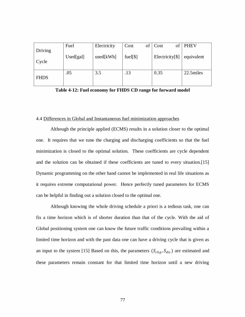
77

Driving

Cycle

Fuel

Used[gal]

Electricity

used[kWh]

Cost of

fuel[$]

Cost of

Electricity[$]

PHEV

equivalent

FHDS .05 3.5 .13 0.35 22.5miles

Table 4-12: Fuel economy for FHDS CD range for forward model

4.4 Differences in Global and Instantaneous fuel minimization approaches

Although the principle applied (ECMS) results in a solution closer to the optimal

one. It requires that we tune the charging and discharging coefficients so that the fuel

minimization is closed to the optimal solution. These coefficients are cycle dependent

and the solution can be obtained if these coefficients are tuned to every situation.[15]

Dynamic programming on the other hand cannot be implemented in real life situations as

it requires extreme computational power. Hence perfectly tuned parameters for ECMS

can be helpful in finding out a solution closed to the optimal one.

Although knowing the whole driving schedule a priori is a tedious task, one can

fix a time horizon which is of shorter duration than that of the cycle. With the aid of

Global positioning system one can know the future traffic conditions prevailing within a

limited time horizon and with the past data one can have a driving cycle that is given as

an input to the system [15] Based on this, the parameters (𝑆𝑐𝑕𝑔 , 𝑆𝑑𝑖𝑠 ) are estimated and

these parameters remain constant for that limited time horizon until a new driving

78

schedule. This way one can find out the parameters and tune it so that the instantaneous

minimization principle can be realized as a global solution.

79

CHAPTER FIVE:CONCLUSIONS AND FUTURE WORK

In this dissertation, modeling and simulation of a Plug-in hybrid electric vehicle is

carried out using instantaneous optimization technique. The technique used can be

applied real time online and is computationally less extensive when compared to global

optimization tools. The ECMS strategy implemented for both Forward and backward

models provided us with solutions that optimally split power amongst the actuators by

moving the operating points to points where fuel consumption is minimized. The vehicle

is operated in charge depletion mode until it reaches a charge sustenance mode This

enables us to operate the vehicle in all electric range as far as possible and hence reduces

the emissions. If the trip length were small and the engine never operates, the vehicle is

said to travel using the off-board electrical energy through the grid. Once the vehicle

enters the charge sustaining pattern, the ECMS strategy is implemented. The engine

ON/OFF strategy is also implemented and hence the vehicle can be turned off in case the

engine is idle for certain amount of time. This considerably reduces the fuel consumption

during instances when electrical energy can be used solely to provide the vehicle with the

necessary power. The vehicle is also operated in charge depletion range and the mileage

or miles that the vehicle can run if the vehicle were to operate without the engine turning

on is tabulated. The all electric range considers engine turning on only when the power

demand is more than the threshold that motor can provide. The use of power split

configuration helps us in optimizing the engine performance.

80

The drive cycles used here are the normal city and highway cycles( UDDS and FHDS

cycles). In reality the parameters that are to be optimized or tuned in ECMS have to

comply with the future driving conditions and hence with the aid of GPS(global

positioning system), a real time driving scenario can be simulated. This can be of very

short durations and is simulated using past and future data. This can be fed to the vehicle

controller to optimize or tune the parameters for that cycle. And also the future work

includes simulating a blended strategy which enables us to minimize the fuel

consumption further. This does not include a charge depletion charge sustaining(CDCS)

strategy separately and the vehicle starts from the maximum state of charge of RESS

directly using blended mode. This makes the engine to operate at maximum efficiency

points even in the charge depletion range which had to be compromised in the CDCS

strategy. To realize this mode of operation, one has to tune the charging and discharging

parameters used in ECMS separately and these may have some relation with the trip

length. The future research in this area will throw more light into subsequent

improvement.

81

82

APPENDICES

83

Appendix A:

Nomenclature:

SOC State of Charge of Battery

𝑝𝑤𝑟𝑠𝑡𝑎𝑟𝑡 −𝑒𝑛𝑔𝑖𝑛𝑒 Power to start engine

𝑝𝑤𝑟𝑀𝐺2 Power of Motor/Generator predominantly acting as motor

𝑝𝑤𝑟𝑀𝐺1 Power of Motor/Generator predominantly acting as Generator

𝜔𝑒𝑛𝑔 Engine speed

𝜔𝑖𝑐𝑒 Engine speed

𝜔𝑒𝑛𝑔 −𝑖𝑑𝑙𝑒 Idle speed of Engine

𝜔𝑒𝑛𝑔 −𝑐𝑢𝑟𝑟𝑒𝑛𝑡 Current Engine Speed

𝜔𝑒𝑛𝑔 −𝑜𝑝𝑡 Optimal Engine speed

𝑝𝑤𝑟𝑟𝑒𝑞 Power Request

𝑝𝑤𝑟𝑒𝑛𝑔 Engine Power

𝑝𝑤𝑟𝑒𝑛𝑔−𝑜𝑝𝑡 Optimal Engine power

𝑝𝑤𝑟𝑀𝐺2−𝑜𝑝𝑡 Optimal Power of Motor/Generator predominantly acting as

motor

𝑝𝑤𝑟𝑀𝐺1−𝑜𝑝𝑡 Optimal Power of Motor/Generator predominantly acting as

Generator

𝑚 𝑓 ,𝐼𝐶𝐸 Fuel Consumption rate of Engine

𝑚 𝑓 ,𝐼𝐶𝐸−𝑜𝑝𝑡 Fuel Consumption rate of Engine(Optimal Value)

𝑚 𝑓 ,𝑒𝑞𝑏 Equivalent Fuel consumption rate of Battery

𝑚 𝑓 ,𝑒𝑞𝑏 −𝑜𝑝𝑡 Equivalent Fuel consumption rate of Battery(Optimal Value)

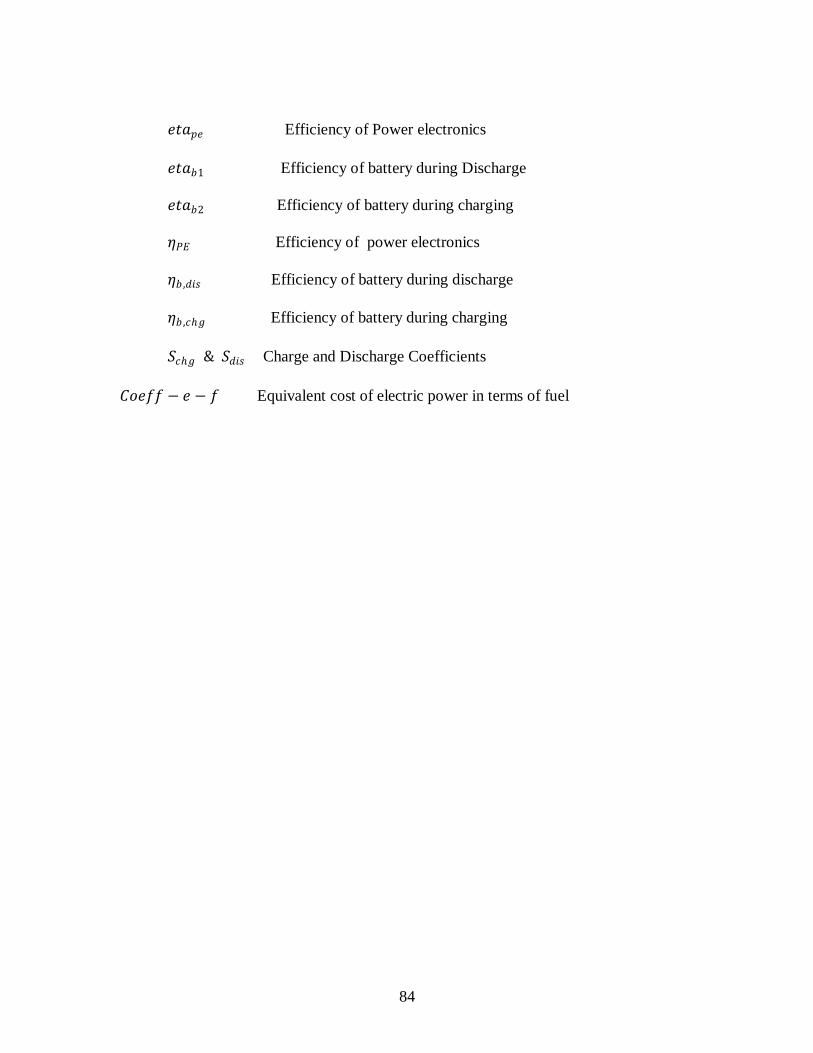
84

𝑒𝑡𝑎𝑝𝑒 Efficiency of Power electronics

𝑒𝑡𝑎𝑏1 Efficiency of battery during Discharge

𝑒𝑡𝑎𝑏2 Efficiency of battery during charging

𝜂𝑃𝐸 Efficiency of power electronics

𝜂𝑏 ,𝑑𝑖𝑠 Efficiency of battery during discharge

𝜂𝑏 ,𝑐𝑕𝑔 Efficiency of battery during charging

𝑆𝑐𝑕𝑔 & 𝑆𝑑𝑖𝑠 Charge and Discharge Coefficients

𝐶𝑜𝑒𝑓𝑓 − 𝑒 − 𝑓 Equivalent cost of electric power in terms of fuel

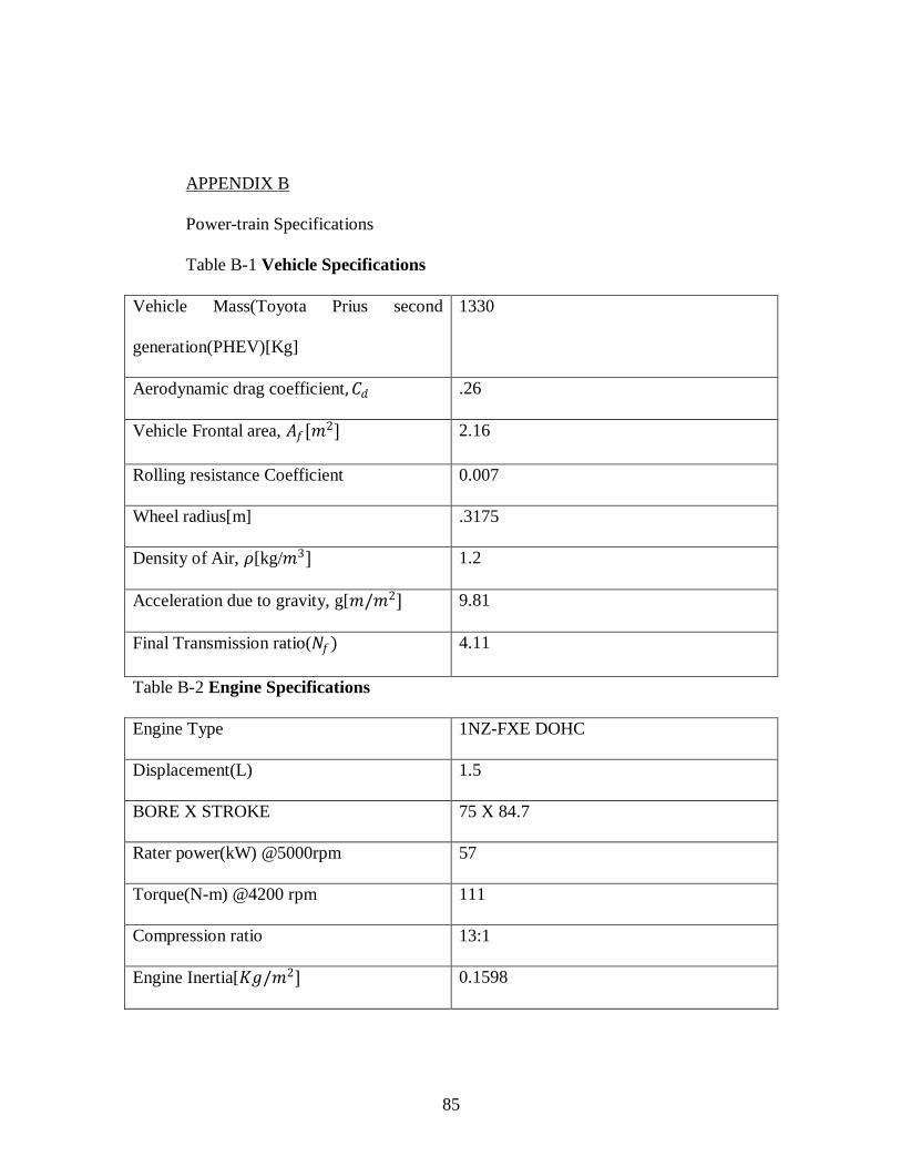
85

APPENDIX B

Power-train Specifications

Table B-1 Vehicle Specifications

Vehicle Mass(Toyota Prius second

generation(PHEV)[Kg]

1330

Aerodynamic drag coefficient,𝐶𝑑 .26

Vehicle Frontal area, 𝐴𝑓[𝑚2] 2.16

Rolling resistance Coefficient 0.007

Wheel radius[m] .3175

Density of Air, 𝜌[kg/𝑚3] 1.2

Acceleration due to gravity, g[𝑚/𝑚2] 9.81

Final Transmission ratio(𝑁𝑓) 4.11

Table B-2 Engine Specifications

Engine Type 1NZ-FXE DOHC

Displacement(L) 1.5

BORE X STROKE 75 X 84.7

Rater power(kW) @5000rpm 57

Torque(N-m) @4200 rpm 111

Compression ratio 13:1

Engine Inertia[𝐾𝑔/𝑚2] 0.1598

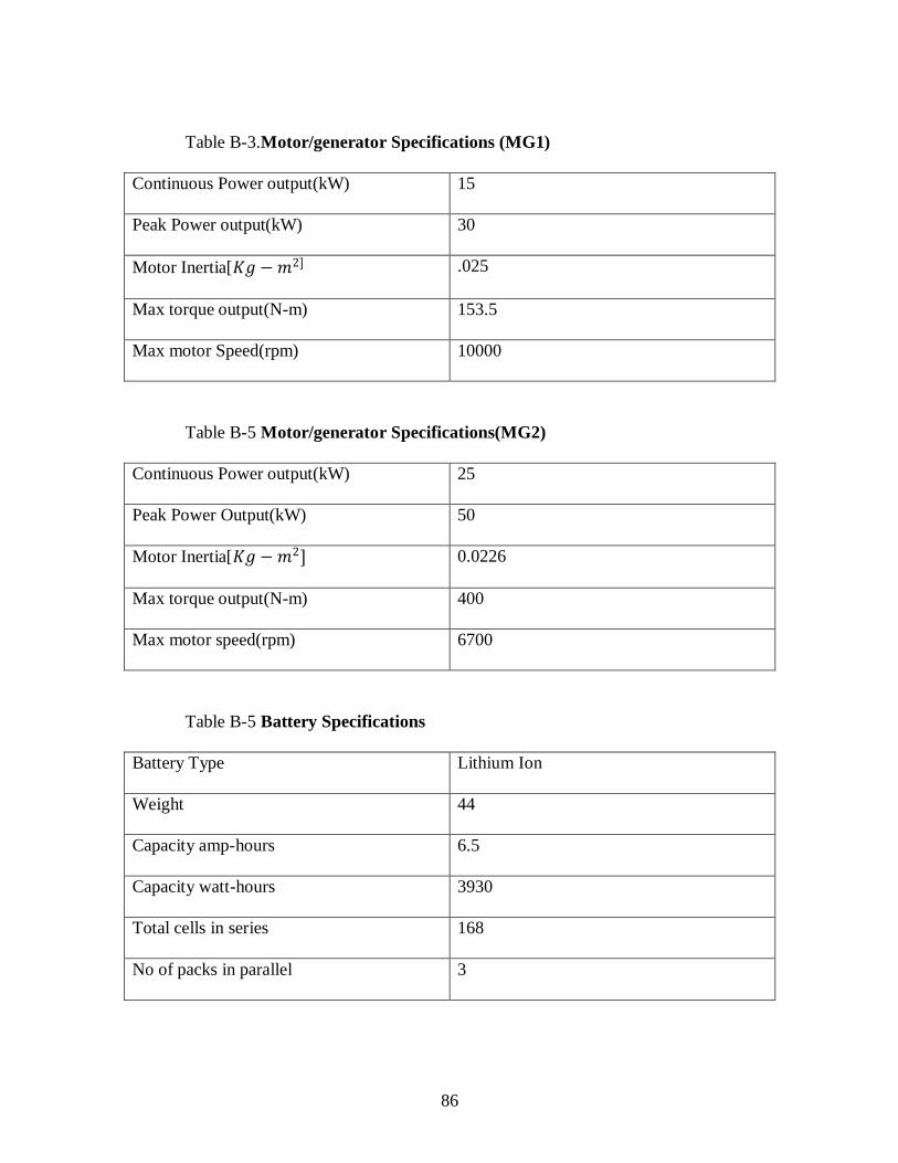
86

Table B-3.Motor/generator Specifications (MG1)

Continuous Power output(kW) 15

Peak Power output(kW) 30

Motor Inertia[𝐾𝑔 − 𝑚2] .025

Max torque output(N-m) 153.5

Max motor Speed(rpm) 10000

Table B-5 Motor/generator Specifications(MG2)

Continuous Power output(kW) 25

Peak Power Output(kW) 50

Motor Inertia[𝐾𝑔 − 𝑚2] 0.0226

Max torque output(N-m) 400

Max motor speed(rpm) 6700

Table B-5 Battery Specifications

Battery Type Lithium Ion

Weight 44

Capacity amp-hours 6.5

Capacity watt-hours 3930

Total cells in series 168

No of packs in parallel 3

87

REFERENCES

[1] S. J. Moura, H. K. Fathy, D. S. Callaway, and J. L. Stein, “A stochasticoptimal

control approach for power management in plug-in hybrid electric vehicles,” Proceedings

of the 2008 ASME Dynamic Systems and Control Conference, 2008.

[2]S.R.Chnek, K.E.Builey. “Regenerative Brvlang System for a hybrid Electric Vehicle”.

Proceeding of the American Control Conference. Anchorage, AK. 2002, “014, pp.3 129-

3134.

[3] Pierluigi Pisu, Kerem Koprubasi and Giorgio Rizzoni, Fellow, IEEE “Energy

Management and Drivability Control Problems for Hybrid Electric Vehicles ” 44th IEEE

Conference on Decision and Control, and the European Control Conference 2005

Seville, Spain, December 12-15, 2005

[4] G. Paganelli, M. Tateno, A. Brahma, G. Rizzoni, and Y. Guezennec “Control

development for a hybrid-electric sport-utility vehicle: Strategy implementation and field

test results,” in Proc. American Control Conference, Arlington, VA, 2001, pp. 5064–

5069.

[5] G. Paganelli, G. Ercole, A. Brahma, Y. Guezennec, and G. Rizzoni, “General

supervisory control policy for the energy optimization of charge-sustaining hybrid

electric vehicles,” JSAE Review, vol. 22, pp. 511–518, 2001.

[6] P. Pisu, C. Musardo, B. Staccia, and G. Rizzoni. “A Comparative Study of

Supervisory Control Strategies for Hybrid Electric Vehicles”. IMECE 2004, 13-19

November 2004, Anaheim, CA.

88

[7] P. Pisu, G. Rizzoni, and E. Calo’. “Control Strategies for Parallel Hybrid Electric

Vehicles”. IFAC’04, Salerno, Italy, 19-23 April 2004, pp.508-513.

[8] Carlson, E., P. Kopf, and J. Sinha, Fuel Cell seminar. 2005, TIAX LLC: Cambridge MA.

[9] Lin C., Peng H., Grizzle J.W., Kang J., “Power Management Strategy for a Parallel

Hybrid Electric Truck”, IEEE Transactions on Control Systems Technology, Vol. 11,

No. 6,November 2003

[10] Brahma A., Guezennec Y., Rizzoni G., “Dynamic Optimization of

Mechanical/Electrical Power Flow in Parallel Hybrid Electric Vehicles”, Proceedings of

the 5th International Symposium in Advanced Vehicle Control, Ann Arbor, MI, USA,

2000

[11] Sharer, P. B., Rousseau, A., Karbowski, D., 2008, "Plug-in Hybrid Electric Vehicle

Control Strategy: Comparison between EV and Charge-Depleting Options," SAE Paper

2008-01-0460, 2008 SAE World Congress.

[12] Rousseau, A., Pagerit, S., and Gao, D., 2007, "Plug-in HybridElectric Vehicle

Control Strategy Parameter Optimization,"Electric Vehicle Symposium-23, Anaheim, CA.

[13] C. GOKCE, “Modeling and Simulation of a Series Parallel Hybrid Electrical

Vehicle”, Master Thesis, Institute of Science andTechnology, Istanbul Technical

University, Istanbul 2005.

[14] Jinming Liu, PhD thesis “Modeling, Configuration And Control Optimization Of

Power-Split Hybrid Vehicles”, University of Michigan 2007.

89

[15] An Adaptive Algorithm For Hybrid Electric Vehicles Energy Management,

Technical Paper For Students And Young Engineers- FISITA WORLD AUTOMOTIVE

CONGRESS, BARCELONA 2004 -

[16] http://www.cleangreencar.co.nz/info_toyota-prius-technical.asp

[17] Zhang, Chen, Vahidi, Ardalan, Li, Xiaopeng, and Essenmacher, Dean, "Role of Trip

Information Preview in Fuel Economy of Plug-in Hybrid Vehicles" to appear in

Proceedings of ASME Dynamic Systems and Control Conference, Hollywood, CA, 2009.

[18] http://www.eia.doe.gov/oog/info/gdu/gasdiesel.asp

[19] http://www.eia.doe.gov/cneaf/electricity/epm/epm_sum.html

[20] Jeffrey Gonder and Tony Markel, National Renewable Energy Laboratory, “Energy

Management Strategies for Plug-In Hybrid Electric Vehicles”, SAE TECHNICAL PAPER

SERIES 2007-01-0290

[21] Phillip B. Sharer, Aymeric Rousseau, Dominik Karbowski and Sylvain Pagerit,

Argonne National Laboratory, Plug-in Hybrid Electric Vehicle Control Strategy:

Comparison between EV and Charge-Depleting Options, SAE TECHNICAL PAPER

SERIES 2008-01-0460

[22] Richard W. Carlson, Michael J. Duoba, Theodore P. Bohn and Anantray D. Vyas,

Argonne National Laboratory, Testing and Analysis of Three Plug-in Hybrid Electric

Vehicles, SAE TECHNICAL PAPER SERIES 2007-01-0283

90

[23] Pesaran, A.A., Vlahinos, A., and Burch, S.D.,"Thermal Performance of EV and

HEV Battery Modules and Packs," Proceedings of the 14th

International Electric Vehicle Symposium, Orlando

FL, December 15–17, 1997.