MODELING AND FORECASTING THE BRAZILIAN TERM STRUCTURE OF INTEREST RATES BY AN EXTENDED NELSON-SIEGEL CLASS OF

MODELS: A QUANTILE AUTOREGRESSION APPROACH*

Rafael B. Rezende§ Mauro S. Ferreira¶

May 18, 2008₣

ABSTRACT

Introducing a five factor more flexible model this paper verifies the in-sample fitting and the out-of-sample forecasting performance of several extensions of the Nelson and Siegel (1987) parametric model which was reinterpreted by Diebold and Li (2006). We used different rules for fixing the parameters λ that govern the models´ exponential components shapes, and predictions were made for different time horizons using different methods. We highlight the Quantile Autoregressive – QAR. The results showed that the five factor model presents a much better in-sample fitting, specially in the short and long term maturities of the term structure. Despite this, a greater predictive power is not guaranteed. It is also shown that, depending on the forecasting horizon, different values of the parameters λ can be optimally fixed. We also conclude that the Brazilian term-structure forecasts performed by the QAR estimated in the median are much more accurate than those performed by the autoregressive methods based on mean-regressions. It shows the robustness of the quantile regression models. Keywords: Term structure of interest rates, in-sample fitting, out-of-sample forecasts, Nelson-Siegel class models, five factor model, outliers, Quantile Autoregression.

JEL Classification: C53, E43, E47.

* This work is based on the first chapter of the master thesis of Rafael B. Rezende at CEDEPLAR. Comments and suggestions are welcome. The views expressed are those of the authors and do not reflect those of FIEMG. Any remaining errors are our responsibility only. § CEDEPLAR – Center for Development and Regional Planning, Belo Horizonte, Brazil. e-mail: rafabarrosrezende@hotmail.com. Tel: 55 31 21270644. ¶ FIEMG – Federation of the Industries of the State of Minas Gerais and CEDEPLAR, Belo Horizonte, Brazil. e-mail: mauro.ferreira@fiemg.com.br. Tel: 55 31 32634385. ₣ This version. First version: April 10, 2008.

1

1 INTRODUCTION

In the last three decades the modeling and the estimation of the term structure of

interest rates have achieved important advances. Several theoretical and econometric

models have been developed, which, basically, can be grouped in three classes. The first

class concerns the so-called equilibrium models. Its tradition focuses on modeling the

dynamics of the short-term rates, typically using affine models, after which yields at other

maturities can be derived with the help of a diffusion process. The main representatives of

this class are the models developed by Vasicek (1977), Cox et al. (1985) and Duffie and

Kan (1996). The second class brings together the no-arbitrage models specially described

by Hull and White (1990) and Heath et al. (1992). They are developed from the imposition

of no-arbitrage conditions between the current yield curve rates. These restrictions generate

its perfect fit. They are particularly used for asset pricing.

Alternatively it is possible to model the term structure of interest rates without

imposing the equilibrium and the no-arbitrage conditions. This is how the third class,

constituted by the so-called statistical or parametric models, works. Included in this class

are the Litterman and Scheinkman (1991) factor analysis model, the quadratic and cubic

splines interpolation models of McCulloch (1971, 1975), the exponential and smoothing

splines of Vasicek and Fong (1982) and Fisher et al. (1995), respectively, and the Nelson

and Siegel (1987) (NS in the remainder of the paper), Svensson (1994) (SV in the

remainder of the paper), Bliss (1997a) (BL in the remainder of the paper), Björk and

Christensen (1999) (BC in the remainder of the paper) and Almeida, Duarte and Fernandes

(1998) parametric models1. The relevance of this last class in modeling the term structure is

shown by the Bank for International Settlements - BIS (2005). Its study suggests that

fourteen of the fifteen central banks examined2 use parametric models for the construction

of zero-coupon yield curves, and that nine of them make use of the NS model and/or the SV

model.

1 In a recent paper, however, Chistensen, Diebold and Rudebusch (2007) introduced the no-arbitrage restrictions to the Nelson-Siegel model. 2 Belgium, Canada, Finland, France, Germany, Italy, Japan, Norway, Spain, Sweden, Switzerland, United Kingdom and United States.

2

Despite the progress in the development of term structure theoretical models as well

as in the yield curve modeling, little attention has been given to a no less relevant issue: its

forecast. Fixed income portfolio managers can make use of this information to balance their

positions and to mark to market, while risk managers can use it to build strategies of

portfolio immunizations. On the other hand, macroeconomists are interested in issues

related to the practice of monetary policy and in the formulation of macroeconomic

policies. Thus, the development of models specially used to predict the term structure of

interest rates shows to be important and a recent literature has focused on this issue.

Although the equilibrium models are concerned with the dynamics of interest rates

targeted by short-term rates, and are directly linked to the forecasting practice, Dufee

(2002) shows, for American Treasury bonds data, that the Vasicek (1977) and Cox et al.

(1985) models present low predictive power3. The models based in no-arbitrage restrictions

also have little to say about the dynamics and forecasts of the term structure of interest

rates. Because they are specialised in fitting the yield curves at a particular point in time,

such models do not allow its forecast directly. The parametrics, however, have shown good

predictive power. Using monthly American Treasury bonds data, Diebold and Li (2006)

proposed a model (DL in the remainder of the paper) to predict the term structure by the NS

model, reinterpreting its parameters as components of level, slope and curvature, as in

Litterman and Sheinkman (1991). These components, also known as latent factors, are

obtained estimating period by period a cross-sectional OLS regression of the yields on the

exponential components of the NS model. Unlike the Litterman and Sheinkman (1991)

model in which both the factor loadings and the factors are obtained in the estimation

process of the model, in the DL methodology, the so-called factor loadings, represented by

the exponential components, are imposed when the parameter that controls either the

decaying rate of the slope factor loading as the maximum point of the curvature factor

loading is fixed. Predicting the factors through an autoregressive (AR(1)) model the authors

achieved good forecasting results for the American term structure. These results were

3 However, using American economy data, Ang and Piazzesi (2003) show that the no-arbitrage restrictions imposition and the insertion of macroeconomic variables improves the forecasts of an equilibrium model. Since then, many studies with free-arbitrage macro-finance equilibrium models were presented. We can cite Rudebusch and Wu (2003), Hördahl et al. (2005), Mönch (2005), Wu (2005) and, in Brazil, Matsumura and Moreira (2006). All them verifies the predictive improvement of this class of models as Ang and Piazzesi (2003) affirm.

3

compared with those obtained from other forecasting methods applied directly on the yields

of the curves. The competing methods were: Autoregressive Vector (VAR(1)), AR(1),

random walk, Fama and Bliss (1987) forward rate regression, Cochrane and Piazessi (2002)

forward curve regression and the slope regression.

The Diebold and Li (2006) model encouraged the development of others which

sought both replicate it as extend it. For a Canadian zero-coupon interest rate data, Bolder

(2006) compares the DL model with five other, examining both the in sample fitting as the

out of sample forecasting results. Besides the DL model, three affine and two other

parametric models are analyzed. The parametrics are the exponential spline of Li et. al

(2001) and the Fourier series suggested by Bolder (2002). The author concludes that the DL

model presents both a better in sample fitting as a greater predictive power, showing,

however, its difficulties in generating better forecasts than a random walk. De Pooter

(2007), with the same data used by Diebold and Li (2006), examines various parametric

models of the NS class: DL with two and three factors, BL, BC, SV and an adjusted-SV

proposed by the author, comparing both their in-sample fitting ability as their predictive

power. The author applies several estimation methods, and concludes that the more flexible

models of four factors (BC, SV and adjusted-SV) capture various yield curves shapes,

presenting better in-sample fitting and out-of-sample forecasting performance4. In a recent

paper Chistensen, Diebold and Rudebusch (2007) introduced no-arbitrage restrictions to the

NS model on a dynamic way. The authors show that these restrictions improve the in-

sample fitting and the out-of-sample forecasting performance of the model. Some papers

has sought add macroeconomic variables to the DL model seeking a relationship between

them and the term structure. We can cite Diebold, Rudebusch and Aruoba (2006) and

Diebold, Piazzesi and Rudebusch (2005).

In Brazil, using a daily ID5-Future data, Varga (2007) mirrors the Diebold and Li

(2006) work, finding that simplest structures like random walk, AR(1), VAR(1) and slope

regression present a greater predictive power than the parametric model. Vicente and Tabak

(2007), for a Brazilian swaps data, compared the DL model with an affine model and a

random walk, concluding that the first provides superior forecasts, especially for long time

4 Specially the BC, that is easier to be estimated. 5 The Interbank Deposits (ID) rate is the weighted average of the Interbank lending operations rates for a day.

4

horizons and for short-term interest rates. Almeida et. al (2007a) using a daily ID-Future

data, propose an extension of DL based on the SV model and conclude that the

incorporation of a double curvature factor raises the model´s predictive power. Almeida et.

al (2007b), with the same previous data, examine how the DL predictive power is affected

by the imposition of different factor loadings. They conclude that, for four different

forecasting horizons, there are optimal loadings capable to minimize the forecasting errors

of the model. Laurini and Hotta (2007), with a daily Brazilian ID-PRE Swap6, show how

Bayesian extensions based on the SV model can improve the forecasting results of the DL.

In this paper, motivated by the results of Almeida et. al (2007b) and De Pooter

(2007), and by the recent developments with the Quantile Autoregression - QAR model of

Koenker and Xiao (2002, 2004, 2006), we analyze the in-sample fitting and the out-of-

sample predictive power of the DL, BL, BC, SV and a proposed five factor (FF in the

remaining of the paper) model, all belonging to the parametric NS class. The FF emerges as

a natural extension of the SV model in an attempt to seek both a better in-sample fitting as a

greater predictive power. The forecasts were generated by the Random Walk (RW),

Autoregressive (AR(1)), Autoregressive Vector (VAR(1)) and Quantile Autoregressive

(QAR(1)) methods and were compared to those of RW, AR(1), VAR(1) and QAR(1),

which were applied directly on the yields of the term structure. Using a Brazilian zero-

coupon data, we have implemented different rules for setting the parameters that determine

the factor loadings shapes. The purpose was to increase the predictive power of the models

and to show that the optimal parameters assume different values depending on the

forecasting horizon. We then have checked if the predictions of the NS models outweigh

those of the competing methods.

The main paper contributions are two. Firstly, the introduction of the FF as a new

NS class model. It is well known in the literature the dificulty of the NS models to fit the

beggining and the ending of the yield curves. Trying to remedy this problem we introduced

a second slope term in the SV model specification observing if this flexibility gain could

improve the in-sample fitting and increase the predictive power of the model. Secondly, the

6 One of the most important and liquid instruments in the Brazilian fixed income market is the ID x PRE Swap. The PRE rate is a fixed coupon rate and ID rate is the Interbank Deposits (ID) rate is the weighted average of the Interbank lending operations rates for a day. This Swap contract has exactly the same characteristics of a zero-coupon bond. Moreover, it is registered and have all the assurances given by the Brazilian Futures and Commodities Exchange - BM&F, and therefore can be considered risk-free.

5

use of the QAR as a term structure forecasting method used in link with the NS class

models. It is argued that the presence of outliers in the data diminishes the predictive power

of the mean-regression methods as the ARIMA7, VAR8 and also the Kalman Filter. Thus,

because it inherits the robustness property of the quantile regression models, the QAR(1),

estimated in the percentile 0.5 (the median), was used to check if it is able to generate more

accurate term structure forecasts.

The results show that the proposed five factor model is more flexible and better

capture the in-sample movements of the Brazilian term structure. The fitting errors at the

the short term and long term maturities were substatially reduced. When the out-of-sample

forecasts are analyzed we conclude that the FF do not improve the results reached by the

other NS models. The SV was the best, followed by the BL and the BC. We also show that

the SV, BC, BL and the FF outweigh the forecasting abilities of simpler structures such as

the random walk and the other Autoregressive models, especially for long time horizons.

Another conclusion was that the different fixing rules for the factor loadings may influence

the out-of-sample forecast results. It supports the Almeida´s et. al (2007b) idea that,

depending on the forecasting horizon, different values for the parameters of the loadings

should be fixed. Finally, we show that the QAR(1) forecasts are more accurate than those

of other methods, especially for long time horizons.

The remainder of the paper is organized as follows. The second section presents the

NS models which will be analyzed in the paper; the third discusses the data used in the

estimation; in the fourth section the estimation of the NS term structure models are

addressed, as well the different out-of-sample forecasting methods and the different rules

used for setting the decaying parameters of the exponential components of the models; the

fifth section presents the fitting and the forecasting results; and the sixth section concludes

the paper.

2 NELSON-SIEGEL CLASS MODELS

7 Ledolter (1989) and Hotta (1993) argue that the presence of outliers induces the appearance of bias in the parameters of ARIMA models, reducing its out of sample forecasts quality. 8 For VAR the effect can be even worse than for the ARIMA model. The extreme values observed in series can induce the appearance of outliers in all regressions of the model, affecting the robustness of the estimates and its forecast quality.

6

The term structure of interest rates can be described in terms of the spot (or zero-

coupon) rate, the discount rate and the forward rate. The forward curve determines rates as

a function of maturities. A forward rate is the interest rate of a forward contract on an

investment which will be initiated τ periods in the future and which will mature *τ periods

beyond the start date of the contract. We obtain the instantaneous forward rate ( )τf by

letting the maturity of such forward contract go to zero: ( ) ( )ττττ

ff =→

,lim *

0* .

From the instantaneous forward rates, we get the forward yield curve, ( )τf .

We can then determine the spot rate implicit in a zero-coupon bond with maturity

τ , ( )τy . Under continuous compounding, taking an average of forward rates, we get the

spot rate:

∫=τ

ττ

0

)(1

)( dxxfy (2.1)

Then, from the spot rates, we get the spot yield curve, ( )τy .

The discount curve is made by rates which gives the present value of a zero-coupon

bond that pays a nominal value of $1.00 after τ periods. It can be obtained from the spot

curve through the following relationship:

τττ )()( yed −= (2.2)

From the equations above we can then relate the discount and the forward curves by

the following formulas:

−= ∫

τ

τ0

)(exp)( dxxfd (2.3)

)(

)()(

'

τ

ττ

d

df −= (2.4)

7

We can move from a curve to the other using the relationships specified above.

2.1 THREE FACTOR BASE MODEL

Nelson and Siegel (1987) suggest to fitting the forward curve at a particular point in

time using the following parametric model:

( ) λτλτ λβββτ −− ++= eef 321 (2.5)

From (2.4) we can get the spot yield curve:

( )

−

−+

−+= −

−−λτ

λτλτ

λτβ

λτββτ e

eey

11321 (2.6)

where the constant λ governs the decaying speed of the 2β ´s exponential component and

the maximum point of the 3β ´s exponential component. Thus λ governs the decay rate of

the whole curve.

Although the NS model has been designed as a static model, Diebold and Li (2006)

reinterpreted it as a dynamic one. Estimating period by period the yields on the exponential

components of the model, its coefficients became able to change in time, i.e. t1β , t2β , t3β

and tλ , determining the whole term structure in a given period. By the shape of the

components, which can be viewed in Figure 1 (a), the authors interpreted them as factor

loadings and the series of the estimated coefficients as level, slope and curvature factors.

Despite tλ be a time-varying parameter, the authors fixed it. By doing so, the model

becomes linear and can then be estimated using a straightforward cross-sectional OLS.

Although the basic model captures many yield curves shapes, it can not deal with all

the shapes that the term structure assumes over time, especially in the emerging markets,

where the yield curves uses to appear twisted, with more than one inflection point. To

remedy this problem, several more flexible parametric models of the NS class have been

proposed in the literature, adding additional factors, including other decaying parameters,

8

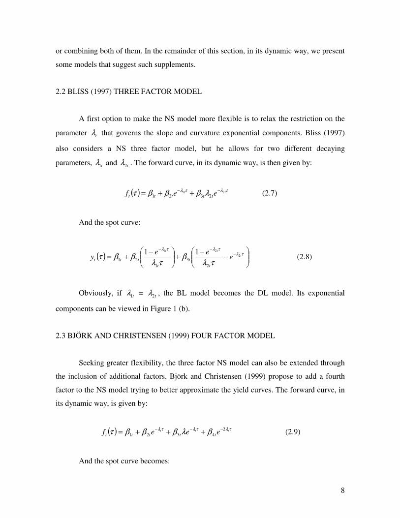
or combining both of them. In the remainder of this section, in its dynamic way, we present

some models that suggest such supplements.

2.2 BLISS (1997) THREE FACTOR MODEL

A first option to make the NS model more flexible is to relax the restriction on the

parameter tλ that governs the slope and curvature exponential components. Bliss (1997)

also considers a NS three factor model, but he allows for two different decaying

parameters, t1λ and t2λ . The forward curve, in its dynamic way, is then given by:

( ) τλτλ λβββτ tt eef ttttt21

2321−− ++= (2.7)

And the spot curve:

( )

−

−+

−+= −

−−τλ

τλτλ

τλβ

τλββτ t

tt

eee

yt

t

t

ttt2

21

2

3

1

21

11 (2.8)

Obviously, if t1λ = t2λ , the BL model becomes the DL model. Its exponential

components can be viewed in Figure 1 (b).

2.3 BJÖRK AND CHRISTENSEN (1999) FOUR FACTOR MODEL

Seeking greater flexibility, the three factor NS model can also be extended through

the inclusion of additional factors. Björk and Christensen (1999) propose to add a fourth

factor to the NS model trying to better approximate the yield curves. The forward curve, in

its dynamic way, is given by:

( ) τλτλτλ βλβββτ ttt eeef ttttt

24321

−−− +++= (2.9)

And the spot curve becomes:

9

( )

−+

−

−+

−+=

−−

−−

τλβ

τλβ

τλββτ

τλτλ

τλτλ

t

t

t

t

t

ttt

t

t

tt ee

eey

2

111 2

4321 (2.10)

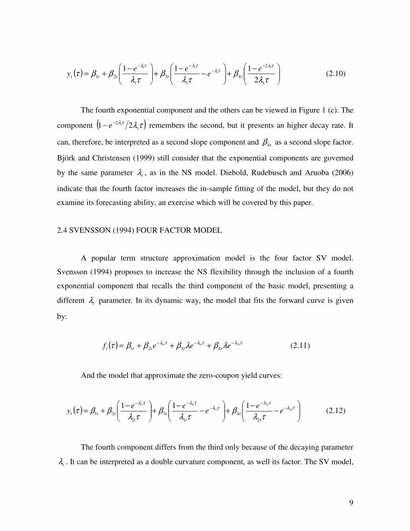
The fourth exponential component and the others can be viewed in Figure 1 (c). The

component ( )τλτλt

te 21 2−− remembers the second, but it presents an higher decay rate. It

can, therefore, be interpreted as a second slope component and t4β as a second slope factor.

Björk and Christensen (1999) still consider that the exponential components are governed

by the same parameter tλ , as in the NS model. Diebold, Rudebusch and Aruoba (2006)

indicate that the fourth factor increases the in-sample fitting of the model, but they do not

examine its forecasting ability, an exercise which will be covered by this paper.

2.4 SVENSSON (1994) FOUR FACTOR MODEL

A popular term structure approximation model is the four factor SV model.

Svensson (1994) proposes to increase the NS flexibility through the inclusion of a fourth

exponential component that recalls the third component of the basic model, presenting a

different tλ parameter. In its dynamic way, the model that fits the forward curve is given

by:

( ) τλτλτλ λβλβββτ ttt eeef ttttt211

4321−−− +++= (2.11)

And the model that approximate the zero-coupon yield curves:

( )

−

−+

−

−+

−+= −

−−

−−τλ

τλτλ

τλτλ

τλβ

τλβ

τλββτ t

t

t

tt

ee

eee

yt

t

t

t

t

ttt2

2

1

11

2

4

1

3

1

21

111 (2.12)

The fourth component differs from the third only because of the decaying parameter

tλ . It can be interpreted as a double curvature component, as well its factor. The SV model,

10

theoretically, fits the various spot curves shapes better then the three factor models. Its

exponential components can be viewed in Figure 1 (d).

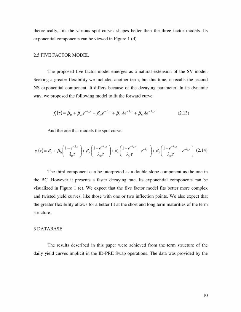
2.5 FIVE FACTOR MODEL

The proposed five factor model emerges as a natural extension of the SV model.

Seeking a greater flexibility we included another term, but this time, it recalls the second

NS exponential component. It differs because of the decaying parameter. In its dynamic

way, we proposed the following model to fit the forward curve:

( ) τλτλτλτλ λβλββββτ tttt eeeef tttttt2121

54321−−−− ++++= (2.13)

And the one that models the spot curve:

( )

−

−+

−

−+

−+

−+= −

−−

−−−τλ

τλτλ

τλτλτλ

τλβ

τλβ

τλβ

τλββτ t

t

t

ttt

ee

eeee

yt

t

t

t

t

t

t

ttt2

2

1

121

2

5

1

4

2

3

1

21

1111 (2.14)

The third component can be interpreted as a double slope component as the one in

the BC. However it presents a faster decaying rate. Its exponential components can be

visualized in Figure 1 (e). We expect that the five factor model fits better more complex

and twisted yield curves, like those with one or two inflection points. We also expect that

the greater flexibility allows for a better fit at the short and long term maturities of the term

structure .

3 DATABASE

The results described in this paper were achieved from the term structure of the

daily yield curves implicit in the ID-PRE Swap operations. The data was provided by the

11

Brazilian Futures and Commodities Exchange - BM&F9. The sample ranges from March

16th 2000 to October 15th 2007, including 1883 working days. Due to the existence of a few

liquid contracts, especially for the long-term maturities, we considered a data with 15

maturities: 1, 2, 3, 4, 5, 6, 7, 8, 9, 12, 18, 24, 36, 48 and 60 months (in running days).

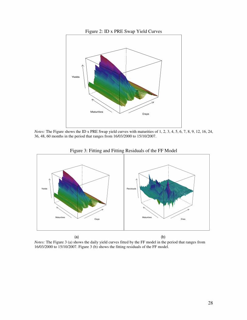
Figure 2 shows the sample yield curves evolution.

The period covered by the sample is very interesting for the analysis, since in

several days the curves are quite twisted, with many different shapes. In addition, they

constantly change their forms from one day to other. These stylized facts allowed us to test

rigorously both the in-sample fitting as the out-of-sample forecasting performances of the

models.

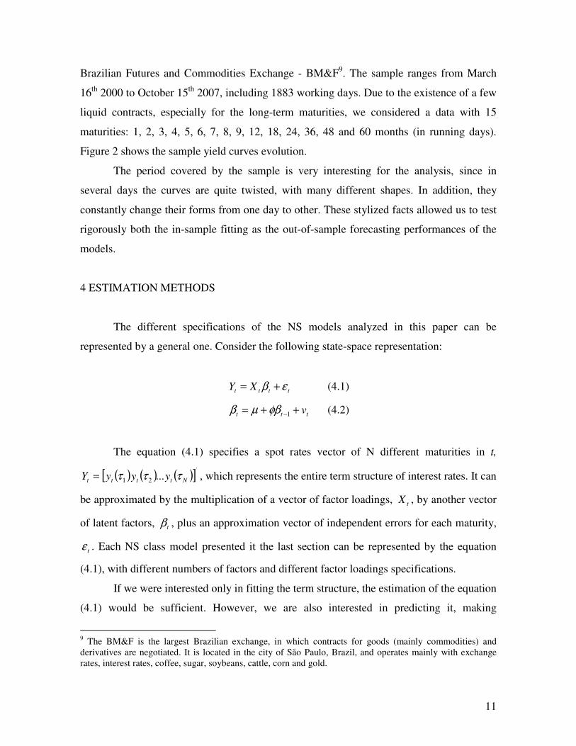
4 ESTIMATION METHODS

The different specifications of the NS models analyzed in this paper can be

represented by a general one. Consider the following state-space representation:

tttt XY εβ += (4.1)

ttt v++= −1φβµβ (4.2)

The equation (4.1) specifies a spot rates vector of N different maturities in t,

( ) ( ) ( )[ ]'

...21 Ntttt yyyY τττ= , which represents the entire term structure of interest rates. It can

be approximated by the multiplication of a vector of factor loadings, tX , by another vector

of latent factors, tβ , plus an approximation vector of independent errors for each maturity,

tε . Each NS class model presented it the last section can be represented by the equation

(4.1), with different numbers of factors and different factor loadings specifications.

If we were interested only in fitting the term structure, the estimation of the equation

(4.1) would be sufficient. However, we are also interested in predicting it, making

9 The BM&F is the largest Brazilian exchange, in which contracts for goods (mainly commodities) and derivatives are negotiated. It is located in the city of São Paulo, Brazil, and operates mainly with exchange rates, interest rates, coffee, sugar, soybeans, cattle, corn and gold.

12

necessary the estimation of the equation (4.2). Following the methodology proposed by

Diebold and Li (2006) we then specify autoregressive models to the factors as in equation

(4.2). We propose the use of the AR(1), VAR(1) and QAR(1). We also make use of the

RW. In that case the equation (4.2) assumes the form htt −= ββ , where h is the forecasting

horizon. This way we have used twenty forecasting models: four forecasting methods for

each NS class model10.

To complete, we assumed that both the errors tε e tv are i.i.d., orthogonal and

normally distributed. The exception occurs when the equation (4.2) is estimated by the

QAR. In that case, no probability distribution is imposed to the error tv , assuming only

independence.

Before describing the estimating and the forecasting methodologies, we will present

a brief discussion about the Quantile Autogressive models.

4.1 QUANTILE AUTOREGRESSION

In three recent papers Koenker and Xiao (2002, 2004, 2006) discuss the so-called

Quantile Autoregressive (QAR) model. In QAR, the ω th quantile functions conditional on

the response variable, ty , is expressed as a linear function of ty . Consider the following

Autoregressive model of order p:

,...11 tptptt uyyy +++= −− αα nt ,...,1= (4.3)

Calling the ω th quantile of tu as )(ωuQ , and the ω th quantile of ty conditional on

ptt yy −− ,...,1 as )...,,( 1 ptty yyQt −−ω , we have:

ptptuptty yyQyyQt −−−− +++= ααωω ...)(),...,( 111 (4.4)

10 They are: NS-RW, NS-AR(1), NS-VAR(1), NS-QAR(1), BL-RW, BL-AR(1), BL-VAR(1), BL-QAR(1), BC-RW, BC-AR(1), BC-VAR(1), BC-QAR(1), SV-RW, SV-AR(1), SV-VAR(1), SV-QAR(1), FF-RW, FF-AR(1), FF-VAR(1), FF-QAR(1).

13

Being )(),...,( 11 −−− = typtty IQyyQtt

ωω , )()(0 ωωα uQ= , 11 )( αωα = ,..., pp αωα =)(

and defining '10 ))(),...,(),(()( ωαωαωαωα p= and '

1 ),...,,1( pttt yyx −−= , we have then:

)()( '1 ωαω tty xIQ

t=− (4.5)

where )1,0(∈ω , and )( 1−ty IQt

ω is the ω th quantile function of ty condicional on past

information ( 1−tI ). This characterizes the quantile autoregressive model of order p, QAR(p).

Solving the following problem we then estimate the linear QAR(p) model:

)(min1

'

1∑−

ℜ∈−

+

n

t

tt yxp

αρτα

(4.6)

The solutions of (4.6) are called quantile autoregressive estimators of order p. Seen

as a function of ω we refer to )(ˆ ωα as the QAR(p) process.

When the purpose is to make forecasts for h periods ahead using the QAR(p) model,

the equation (4.5) becomes )(ˆ)( ' ωαω tty xIQht

=+

, where '),...,( pttt yyI −= and )(ˆ ωα was

estimated by (4.5) assuming '),...,,1( hpthtt yyx −−−= .

In this paper, to forecast the term structure, we make use of the QAR(1) model

estimated in the quantile 0.5 (the median). Relying on the property of robustness of the

quantile regression models, we are interested in checking if the QAR(1) forecasts are more

accurate than those of other autoregressive models.

4.2 IN-SAMPLE FIT

The parameters tλ that govern the behavior of the exponential components of each

model were fixed11 adopting another criterion than Diebold and Li (2006). For NS and BC,

11 If the decaying parameters are not fixed, the daily yields become a non-linear function of the parameters

tλ

e tβ , and therefore, a nonlinear estimation method, such as the Nonlinear Least Squares (NLS), is necessary.

However, Laurini and Hotta (2007) and Gimeno and Nave (2006) argue that the estimation of the NS models

14

in a vector of possible parameters λ , one was chosen. It provided the lowest average term

structure adjustment error, measured by the average of the Root Mean Squared Error -

RMSE. Explaining in a better way, initially a vector of parameters λ was created and, for

each element of that vector, the factor loadings were fixed. We then, for each λ , applied a

daily cross-sectional OLS to the models, obtaining its factors time series. Multiplying the

estimated factors by the pre-fixed loadings we then get the fitted term structure for each NS

model and for each λ . The RMSE was then calculated for each term structure maturity and

its averages was taken. Doing this we have obtained an average term structure RMSE for

each element of the vector of parameters λ , choosing, finally, the one that generates the

lowest RMSE.

The same criteria for the selection of the decaying parameters were adopted to the

BL, SV and FF models. The difference was that two different parameters determine its

factor loadings. Thus many possible combinations between 1λ e 2λ were created, choosing

the one that generated the lowest average RMSE to the fitting of the whole term structure.

The estimation process was also the same.

4.3 OUT-OF-SAMPLE FORECASTS

The out of sample forecasts were made for the horizons of 1 day, 1 week (5 working

days) and 1 month (21 working days). We implemented a two-stage estimation procedure:

first the models were fitted to a sub-sample of the data and its factors were obtained, as

discussed in section 4.2, and then the term structure was predicted modeling the factors

dynamics through the four forecasting methods. The NS models were fitted using the first

1400 observations, and the remaining 483 were used to evaluate their predictive power.

The parameters λ 12 were fixed through four different rules, proposed by Almeida

et. al (2007b). All of them are applied to all the NS class models. In the rule 1, the λ are

by NLS, especially the SV, generates extremely unstable time series for the parameters β , showing that the

term structure forecasts are much more accurate when the tλ are fixed. In this paper, all models were

estimated considering tλ fixed. Thus they became non-time-varying. In the text, we then adopt its notation

without the t, indicating that it is fixed. 12 These parameters refers to a unique parameter λ or to a double

1λ and 2λ , depending on the analyzed

model.

15

chosen to minimize the fitting RMSE of the first 1400 days of the sample. In the rules 2, 3

and 4, the optimal parameters are chosen to minimize the forecasts RMSE of the NS

models for each time horizon and for each forecasting method. Explaining in a better way,

initially, for each λ of a vector of possible optimal parameters, the NS models are

estimated and its factors obtained. Then, the RW and the autogressive processes are fitted

to the first 1400 observations of each factor, using the remaining 483 for the forecasts. The

λ that generate the smallest forecasts RMSE for the 1, 5 and 21 days ahead are then chosen

according to the rules 2, 3 and 4, respectively.

After obtaining the optimal λ and the factors, the out-of-sample forecasts can then

be made for 1 day, 1 week and 1 month horizons using the four forecasting methods. They

are fitted to the first 1400 observations of the factors, leaving the remaining to evaluate the

forecasts.

As we adopted four forecasting methods and four rules for choosing the optimal

decaying parameters, where, in the rule 1, the same parameter is used by the four methods,

we got thirteen optimal parameters or combinations of optimum parameters for each NS

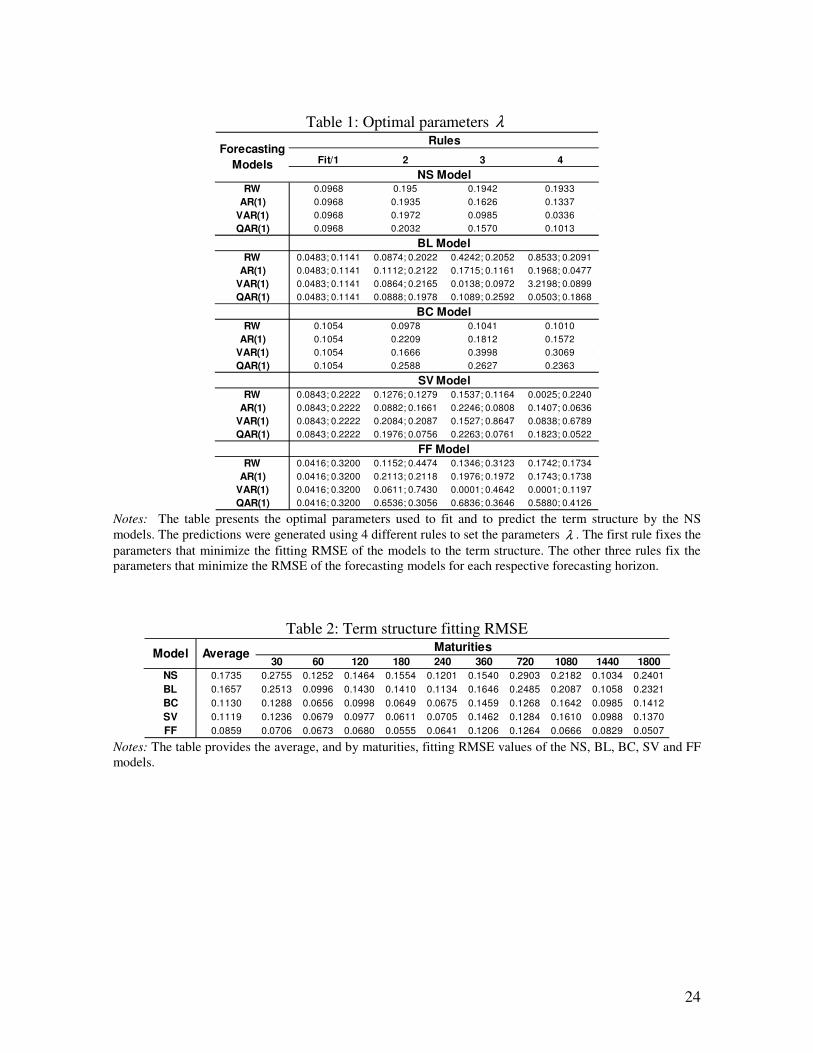
class model, which gives 65 parameters or combinations of parameters in total. The Table 1

shows their values13.

4.3.1 COMPETING MODELS

To test the forecast ability of the NS models, their results were compared with those

of simpler forecasting methods, which were applied directly on the yields of the term

structure. They are:

(1) Random Walk (RW):

)()(ˆ ττ tht yy =+ (4.7)

(2) AR(1) on yield levels

)(ˆ)(ˆ)(ˆ τγττ tht ycy +=+ (4.8)

13 If requested, the authors can provide the vectors from where the optimal parameters were obtained.

16

(3) VAR(1) using the three main principal components of the yields

tht PCCy Γ+=+ˆˆ)(ˆ τ (4.9)

where ],,[ 321 tttt pcpcpcPC = are the first three principal components extracted from the

covariance matrix of the time series of the maturities yields.

(4) QAR(1) on yield levels

)(ˆ)(ˆ)(ˆ 5.05.0 τϕττ ωω tht yqy ==+ += (4.10)

For the VAR(1), the maturities rates were estimated on their first three principal

components with the goal of reducing the number of parameters14 and consequently the

forecasting errors. As the first three components explain over 99% of the total variability of

the daily rates, this procedure seems to be satisfactory.

In all the cases, the competing models were also initially fitted to the first 1400

observations of the sample. The remaining was used to evaluate their forecasts also by the

RMSE criterion.

In the next few sections, the NS class models will be compared evaluating their in-

sample and out-of-sample forecasting performances.

5 EMPIRICAL RESULTS

5.1 IN-SAMPLE FIT

The Table 2 provides the average, and by maturities, term structure fitting errors of

each NS model. Both were measured by the RMSE criterion. Notice that the five factor

model presents a large advantage over the other ones. In all maturities the fitting errors are

substantially reduced, showing the flexibility gain obtained with the inclusion of the second 14 The principal components analysis is a method that reduces the dimensionality of the data, making its interpretation and analysis easier, without a significant loss of information. The basic idea is to generate a new set of variables that are linear combinations of the original and, in addition, are mutually orthogonal. Thus, there is no redundancy of information and in the majority of its applications the first components can explain much of the total variability of the original data. The processed variables are called principal components.

17

slope term. The results also allow us to verify that the new specification seems solving the

puzzle over the NS models: the difficulty to fit the initial and the ending maturities of the

term structure. Clearly the most expressive improvements occurs at the 30 and 1800 days

vertices: it is about 75% and 170%, respectively. From the Table 2 we can notice also an

advantage of the BL over the NS basic model and a small advantage of the SV over BC.

The Figure 3 (a) displays the SV fit to the term structure data. The SV fitting residuals can

be viewed in Figure 3 (b).

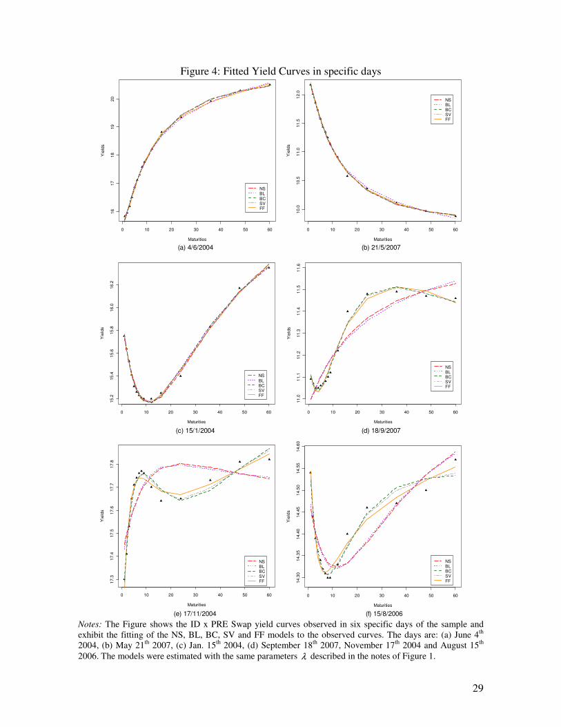
The Figure 4 shows six yield curves examples in specific days of the sample, fitted

by the five NS models. Notice, as we’ve already pointed out, the better fitting results of the

more flexible models, BC, SV and FF. The Figures 4 (a) to (c), where inflection points are

not observed in the curves, exhibit good fitting results to all the models. However, for the

curves that present one or more inflection points we see better fitting results to the more

flexible ones – BC, SV and FF –, as verified in Figure 4 (d) to (f). Nevertheless, there is a

perceived difficulty of the four and five factor models to fit more twisted curves like the

one shown in Figure 4 (f), which presents two inflection points

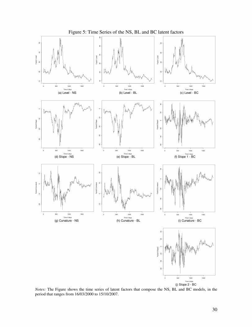
Figure 5 presents the factors time series that have been obtained from the NS

models estimations. They represent the term structure movements. The charts indicate that

the three factor models present very similar series. In contrast the time series of the BC, SV

and FF seem to be quite different. Interesting to note is the smallest persistence observed in

the FF factors, which are shown in Figure 6 together with the SV series.

A fact that draws attention is that the time series of the factors of all the NS models

seem to present many peaks, especially in periods of shocks, such as the confidence crisis

in the pre-election period at the ends of 200115 and the "September 11th attack16". This is an

indication of the possible presence of outliers in the AR(1), VAR(1) and QAR(1)

regressions, which are used to predict the factors of the NS models. In such periods, the

curves seem to have changed too much, a fact that is captured by the time series shown in

Figures 5 and 6.

15 This confidence crisis was the panic that seized markets when the left-leaning Luiz Inácio Lula da Silva was to win the presidency in October, 2001. The confidence crisis occurs around the 650th observation of the data. 16 The “September 11th attack” occurs around the 400th observation of the data.

18

5.2 OUT-OF-SAMPLE FORECASTS

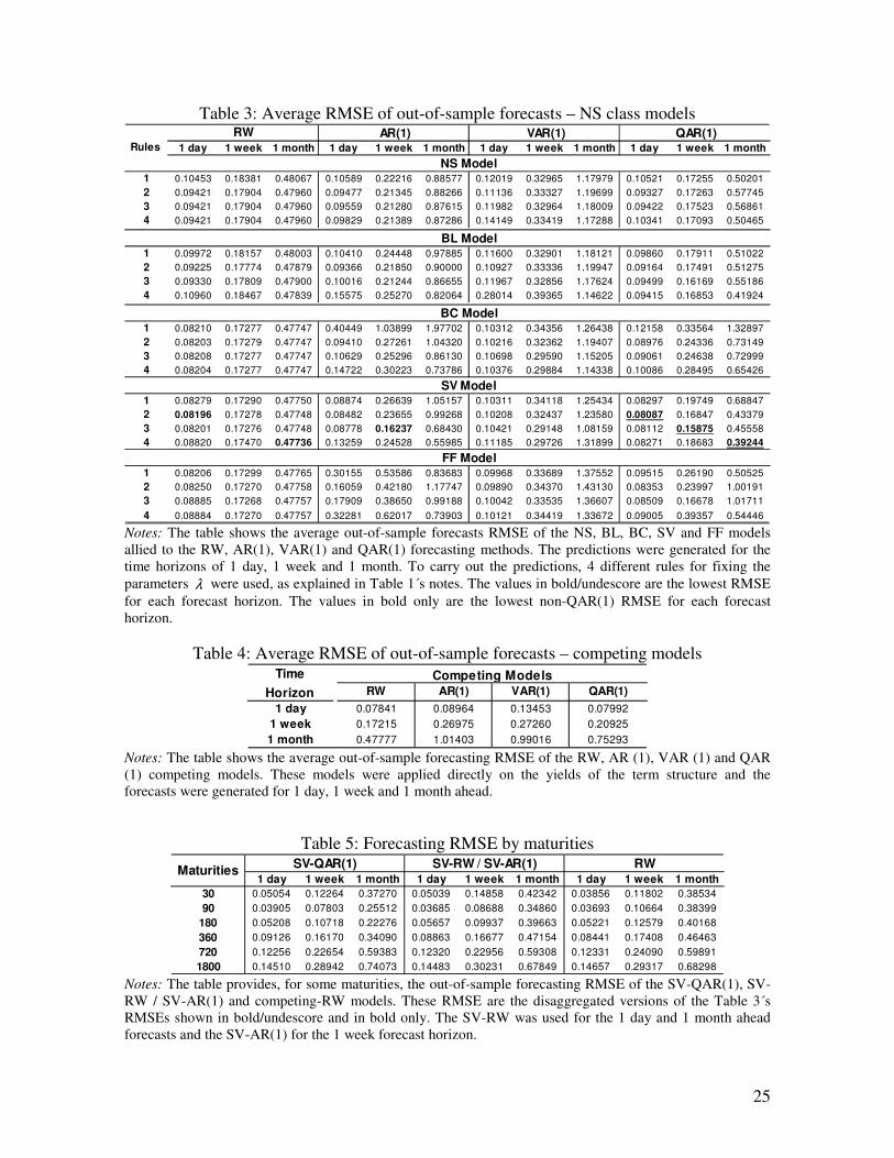
Table 3 shows the term structure average prediction RMSE for each NS class model

and for each forecasting method. Notice that the rules for choosing the optimal parameters

λ make sense. In general, for the rules 2, 3 and 4, the forecasts that presented the lowest

average RMSE were those made for the 1 day, 1 week and 1 month ahead, respectively.

Even working with different data and sample size, this result is similar to that achieved by

Almeida et. al (2007b), validating the hypothesis that the λ ’s values should vary according

to the forecasting horizon.

It is also noticed an advantage of the SV model on the others in most of the rules

and forecasting methods. The other models take turns in the "second place". Interesting to

note is that the greater flexibility obtained with the introduction of the second slope term

does not guarantee a greater forecast ability to the FF model. The second slope term

introduction even deteriorate it. Together with the BC, the FF, except for the RW

forecasting method, showed the worst results.

The Table 4 shows the average forecasting RMSE for each competing model. Note

that the RW is the best. Comparing its results with those obtained by the NS models we

realized that the unique NS models capable of overcoming the RW for the medium and

long horizons are the BC-RW, SV-RW, FF-RW, SV-AR(1), BL-QAR(1), FF-QAR(1) and

SV-QAR(1). Notice that no model is superior than the RW when the forecasts are made for

1 day ahead.

From the Table 3, the results also indicate that the QAR(1) generates more accurate

forecasts than the AR(1) and VAR(1), in general, for all time horizons and NS models. This

advantage is guaranteed by the property of robustness of the quantile regression models,

insofar as the possible presence of outliers in the Autoregressive models seems to be the

generator factor of the low quality of the AR(1) and VAR(1) forecasts. The QAR(1) take

turns with the RW as the best forecasting method for each NS model and time horizon.

However, the best results, which are in bold/undescored, are presented by the SV-QAR(1).

It is followed by the results of the SV-RW (1 day and 1 month horizons) and SV-AR(1) (1

week horizon), which are shown in bold only. Important and interesting to note is the

19

forecast gain obtained by SV-QAR(1) for the 1 month horizon: it generates 20% more

accurate forecasts than the best non-QAR(1) method, the SV-RW.

Table 5 provides, for some maturities, the RMSE of the SV-QAR(1), SV-RW/SV-

AR(1) and RW models´ predictions. These are the broken RMSE versions of the SV-

QAR(1)´s and SV-RW/SV-AR(1)´s RMSEs exhibited in bold/undescored and in bold in

Table 3, and of the RW´s RMSE exhibited in Table 4. We can verify, by maturities, the

superiority of SV-QAR(1) on the other models, specially for the 1 week and 1 month

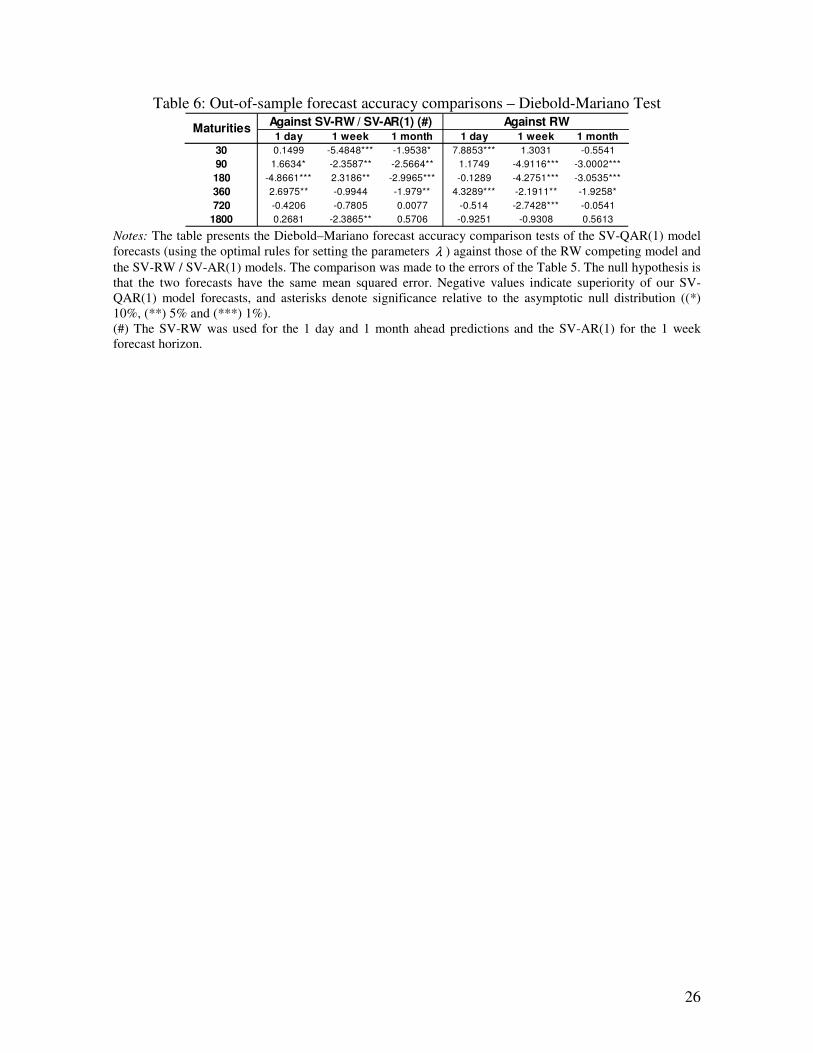
forecasting horizons. This is confirmed by the significant statistics of the Diebold and

Mariano (1995) test, which are exhibited in Table 6. From the Table 5 we can also observe

that, throughout the term structure, the largest predictive errors occur at the end of the yield

curves. The results show that the forecasting errors tend to decrease until a certain short-

term maturity, and then tend to increase until the “long-term” maturity.

6 CONCLUSIONS

This article compares, by the RMSE criterion, the in-sample fit and the out-of-

sample forecasting performances of different NS class models, which can be reinterpreted

as in Diebold and Li (2006). We extended this class introducing a five factor (FF) more

flexible model, which emerges as natural extension of the known SV. As in Almeida et. al

(2007b), we adopted different rules for fixing the parameters that govern the shapes of the

factor loadings of the models. We also used different forecasting methods, highlighting the

QAR(1). The prediction results is compared to those of other forecasting methods which

are applied directly on the yields of the term structure.

The results show the superiority of the proposed five factor models over the other

ones in fitting the term structure, specially in the short and long term maturities. This result

solves the well known problem of the NS class models: their difficulty to fit the beggining

and the ending of the yield curves. We note also a slight advantage of the traditional SV

model over the BC and an advantage of the BL over the NS. Despite the greater flexibility,

as the four factor models, the FF can not fit very well twisted yield curves with two

inflection points. This result instigate the development of parametric models that could

capture these changes fitting more complex yield curves in a better way.

20

Regarding the out-of-sample forecasts, the results indicate that the rules for fixing

the parameters λ make sense, revealing that it is possible to get smaller prediction errors

adjusting them according to the forecasting horizon. This result is similar to that reached by

Almeida et. al (2007b), even for a different data and sample period. We conclude also that

the SV model is, in general, superior than the others, which take turns in the second place.

So, we showed that the greater flexibility achieved by the FF model does not guarantee a

greater predictive power. We note further that the only models capable of overcoming

simpler structures like the RW are the BC-RW, SV-RW, FF-RW, SV-AR(1), BL-QAR(1),

FF-QAR(1) and SV-QAR(1) models. The SV-QAR(1) is the best.

Finally, we conclude that the QAR(1) estimated in the median behaves, in general,

as the best prediction method under review, especially for long time horizons. The property

of robustness of quantile regression methods ensures its high performance in predicting the

term structure, specially in data presenting outliers.

The analysis of this paper can be extended in a number of ways. Firstly, the

imposition of no-arbitrage restrictions as in Christensen, Diebold and Rudebusch (2007)

could be applied to more flexible models like the FF, SV, BC and BL. These models could

be estimated by a robust approach. And secondly, the use of macroeconomic variables

and/or macroeconomic factors as in Diebold, Rudebusch, and Aruoba (2006b) could

improve the forecasts, compared to the yields-only approach that we have used here. All

these topics are part of ongoing research.

REFERENCES

ALMEIDA, C., DUARTE, A., FERNANDES, C. (1998). Decomposing and simulating the movements of term structures in emerging eurobonds markets. Journal of Fixed Income, v. 8, n. 1, p. 21–31.

ALMEIDA, C., GOMES, R., LEITE, A., VICENTE, J. (2007a). Does Curvature Enhance

Forecasting? EPGE Working Paper, Getulio Vargas Foundation. ALMEIDA, C., GOMES, R., LEITE, A., VICENTE, J. (2007b). Movements of the Term

Structure and Criteria of Minimization of Prediction Errors in a Exponencial

Parametric Model. EPGE Working Paper, Getulio Vargas Foundation.

21

ANG. A., M. PIAZZESI (2003). A No-Arbitrage Vector Autoregression of Term Structure Dynamics with Macroeconomic and Latent Variables. Journal of Monetary Economics, v. 50, p. 745–787.

BJORK, T., CHRISTENSEN, B. (1999). Interest Rate Dynamics and Consistent Forward

Rate Curves. Mathematical Finance, v. 9, p. 323–348. BLISS, R. R. (1997). Testing Term Structure Estimation Methods. Advances in Futures

and Options Research, v. 9, p. 197–231. BOLDER, D. J. (2002). Towards a More Complete Debt Strategy Simulation

Framework. Bank of Canada Working Paper, n. 2002–13. BOLDER, D. J. (2006). Modelling Term-Structure Dynamics for Risk Management: A

Practitioner’s Perspective. Bank of Canada Working Paper, n. 2006–48. COCHRANE, J. H., PIAZZESI, M. (2005). Bond risk premia. American Economic

Review, v. 95, 138–160. COX, J., INGERSOLL, J. E., ROSS, S. A. (1985). A Theory of the Term Structure of

Interest Rates. Econometrica, v. 53, p. 385–407. CHRISTENSEN, J., DIEBOLD, F., RUDEBUSCH, G. (2007). The Affine Arbitrage-

Free Class of: Nelson-Siegel Term Structure Models. NBER Working Papers 13611, National Bureau of Economic Research.

DE POOTER, M. (2007). Examining the Nelson-Siegel Class of Term Structure

Models. Tinbergen Institute Discussion Paper, n. TI 2007–043/4. DIEBOLD, F. X., PIAZZESI, M., RUDEBUSCH, G. D. (2005). Modeling Bond Yields in

Finance and Macroeconomics, American Economic Review, v. 95, p. 415–420. DIEBOLD, F. X., LI, C. (2006). Forecasting the Term Structure of Government Bond

Yields. Journal of Econometrics, v. 130, p. 337–364. DIEBOLD, F. X., MARIANO, R. S. (1995). Comparing predictive accuracy. Journal of

Business and EconomicStatistics, v. 13, p. 253–263. DIEBOLD, F. X., RUDEBUSCH G. D., ARUOBA, B. (2006). The Macroeconomy and the

Yield Curve: a Dynamic Latent Factor Approach, Journal of Econometrics, v. 131, p. 309–338.

DUFEE, G. (2002). Term premia and interest rate forecasts in affine models. Journal of

Finance, v. 57, p. 405–443. DUFFIE, D., KAN, R. (1996). A yield-factor model of interest rates. Mathematical

Finance, v. 6, n. 4, p. 379–406.

22

FISHER, M., NYCHKA, D., ZERVOS, D. (1995). Fitting the Term Structure of Interest

Rates with Smoothing Splines. Board of Governors of the Federal Reserve System, Finance and Economics Discussion Series n. 1995–1.

GIMENO, R., NAVE, J. (2006). Genetic Algorithm Estimation of Interest Rate Term

Structure. Documentos de Trabajo del Banco de España, n. 0634. HEATH, D., JARROW, R., MORTON, A. (1992). Bond pricing and the term structure of

interest rates: a new methodology for contingent claims valuation. Econometrica, v. 60, p. 77–105.

HORDAHL, P., TRISTANI, O., VESTIN, D. (2005). A joint econometric model of

macroeconomic and term-structure dynamics. Journal of Econometrics, v. 131, p. 405–444.

HULL, J., WHITE, A. (1990). Pricing interest-rate-derivative securities. Review of

Financial Studies, v. 3, n. 4, p. 573–592. HOTTA, L. K. (1993). The effect of additive outliers on the estimates of aggregated and

disaggregated ARIMA models. International Journal of Forecasting, v. 9, p. 85–93 . KOENKER, R., XIAO, Z. (2002). Inference on the Quantile Regression Process.

Econometrica, v. 70, p. 1583–1612. KOENKER, R., XIAO, Z. (2004). Unit Root Quantile Autoregression Inference. Journal

of the American Statistical Association, American Statistical Association, v. 99, p. 775–787.

KOENKER, R., XIAO, Z. (2006). Quantile Autoregression. Journal of the American

Statistical Association, American Statistical Association, v. 101, p. 980–990. LAURINI, M., HOTTA, L. (2007). Bayesian Extensions of the Diebold and Li Term

Structure Model. IBMEC Working Paper, n. 40. LEDOLTER, J. (1989). The effect of additive outliers on the forecasts from ARIMA

models. International Journal of Forecasting, v. 5, p. 231–240. LI, B., DE WETERING, E., LUCAS, G., BRENNER, R., SHAPIRO, A. (2001). Merrill

Lynch Exponential Spline Model. Merrill Lynch Working Paper. LITTERMAN, R., J. SCHEINKAMN (1991). Common Factors Affecting Bond Returns.

Journal of Fixed Income, v. 1, p. 54–61. McCULLOCH, J. H. (1971). Measuring the Term Structure of Interest Rates. Journal of

Business, v. 44, p. 19–31.

23

McCULLOCH, J.H. (1975). The tax adjusted yield curve. Journal of Finance, v. 30, p. 811–830.

MATSUMURA, M., MOREIRA, A. (2006). Macro Factors and the Brazilian Yield

Curves with no-Arbitrage Models. Institute of Applied Economic Research (IPEA), Discussion Paper n. 1210.

MONCH, E. (2006). Forecasting the Yield Curve in a Data-Rich Environment: a No-

Arbitrage Factor Augmented VAR Approach. European Central Bank Working Paper, n. 544.

NELSON, C. R., SIEGEL, A. F. (1987). Parsimonious Modeling Of Yield Curves. Journal

of Business, v. 60, 473–489. RUDEBUSCH, G. D., WU, T. (2003). A Macro-Finance Model of the Term-Structure,

Monetary Policy, and the Economy. Federal Reserve Bank of San Francisco Working paper, 17.

SVENSSON, L. E. O. (1994). Estimating and Interpreting Forward Interest Rates:

Sweden 1992-1994. NBER Working Paper Series, n. 4871. VARGA, G. (2007). Brazilian (Local) Term Structure Forecast in a Factor Model. VII

Meeting of the Brazilian Finance Society. VASICEK, O. A. (1977). An Equilibrium Characterization of the Term Structure. Journal

of Financial Economics, v. 5, p. 177–188. VASICEK, O. A., FONG, H. G. (1982). Term structure modeling using exponential

splines. Journal of Finance, v. 37, p. 339–348. VICENTE, J., TABAK, B. (2007). Forecasting Bond Yields in the Brazilian Fixed Income

Market. International Journal of Forecasting, v. 1, p. 1–10. WU, T. (2006). Macro Factors and the Affine Term Structure of Interest Rates. Journal of

Money, Credit and Banking, v. 38, n. 7, p. 1847–1875.

24

Table 1: Optimal parameters λ

Fit/1 2 3 4

RW 0.0968 0.195 0.1942 0.1933

AR(1) 0.0968 0.1935 0.1626 0.1337

VAR(1) 0.0968 0.1972 0.0985 0.0336

QAR(1) 0.0968 0.2032 0.1570 0.1013

RW 0.0483; 0.1141 0.0874; 0.2022 0.4242; 0.2052 0.8533; 0.2091

AR(1) 0.0483; 0.1141 0.1112; 0.2122 0.1715; 0.1161 0.1968; 0.0477

VAR(1) 0.0483; 0.1141 0.0864; 0.2165 0.0138; 0.0972 3.2198; 0.0899

QAR(1) 0.0483; 0.1141 0.0888; 0.1978 0.1089; 0.2592 0.0503; 0.1868

RW 0.1054 0.0978 0.1041 0.1010

AR(1) 0.1054 0.2209 0.1812 0.1572

VAR(1) 0.1054 0.1666 0.3998 0.3069

QAR(1) 0.1054 0.2588 0.2627 0.2363

RW 0.0843; 0.2222 0.1276; 0.1279 0.1537; 0.1164 0.0025; 0.2240

AR(1) 0.0843; 0.2222 0.0882; 0.1661 0.2246; 0.0808 0.1407; 0.0636

VAR(1) 0.0843; 0.2222 0.2084; 0.2087 0.1527; 0.8647 0.0838; 0.6789

QAR(1) 0.0843; 0.2222 0.1976; 0.0756 0.2263; 0.0761 0.1823; 0.0522

RW 0.0416; 0.3200 0.1152; 0.4474 0.1346; 0.3123 0.1742; 0.1734

AR(1) 0.0416; 0.3200 0.2113; 0.2118 0.1976; 0.1972 0.1743; 0.1738

VAR(1) 0.0416; 0.3200 0.0611; 0.7430 0.0001; 0.4642 0.0001; 0.1197

QAR(1) 0.0416; 0.3200 0.6536; 0.3056 0.6836; 0.3646 0.5880; 0.4126

BC Model

SV Model

FF Model

Forecasting

Models

Rules

NS Model

BL Model

Notes: The table presents the optimal parameters used to fit and to predict the term structure by the NS models. The predictions were generated using 4 different rules to set the parameters λ . The first rule fixes the parameters that minimize the fitting RMSE of the models to the term structure. The other three rules fix the parameters that minimize the RMSE of the forecasting models for each respective forecasting horizon.

Table 2: Term structure fitting RMSE

30 60 120 180 240 360 720 1080 1440 1800

NS 0.1735 0.2755 0.1252 0.1464 0.1554 0.1201 0.1540 0.2903 0.2182 0.1034 0.2401

BL 0.1657 0.2513 0.0996 0.1430 0.1410 0.1134 0.1646 0.2485 0.2087 0.1058 0.2321

BC 0.1130 0.1288 0.0656 0.0998 0.0649 0.0675 0.1459 0.1268 0.1642 0.0985 0.1412

SV 0.1119 0.1236 0.0679 0.0977 0.0611 0.0705 0.1462 0.1284 0.1610 0.0988 0.1370

FF 0.0859 0.0706 0.0673 0.0680 0.0555 0.0641 0.1206 0.1264 0.0666 0.0829 0.0507

MaturitiesModel Average

Notes: The table provides the average, and by maturities, fitting RMSE values of the NS, BL, BC, SV and FF models.

25

Table 3: Average RMSE of out-of-sample forecasts – NS class models

1 day 1 week 1 month 1 day 1 week 1 month 1 day 1 week 1 month 1 day 1 week 1 month

1 0.10453 0.18381 0.48067 0.10589 0.22216 0.88577 0.12019 0.32965 1.17979 0.10521 0.17255 0.50201

2 0.09421 0.17904 0.47960 0.09477 0.21345 0.88266 0.11136 0.33327 1.19699 0.09327 0.17263 0.57745

3 0.09421 0.17904 0.47960 0.09559 0.21280 0.87615 0.11982 0.32964 1.18009 0.09422 0.17523 0.56861

4 0.09421 0.17904 0.47960 0.09829 0.21389 0.87286 0.14149 0.33419 1.17288 0.10341 0.17093 0.50465

1 0.09972 0.18157 0.48003 0.10410 0.24448 0.97885 0.11600 0.32901 1.18121 0.09860 0.17911 0.51022

2 0.09225 0.17774 0.47879 0.09366 0.21850 0.90000 0.10927 0.33336 1.19947 0.09164 0.17491 0.51275

3 0.09330 0.17809 0.47900 0.10016 0.21244 0.86655 0.11967 0.32856 1.17624 0.09499 0.16169 0.55186

4 0.10960 0.18467 0.47839 0.15575 0.25270 0.82064 0.28014 0.39365 1.14622 0.09415 0.16853 0.41924

1 0.08210 0.17277 0.47747 0.40449 1.03899 1.97702 0.10312 0.34356 1.26438 0.12158 0.33564 1.32897

2 0.08203 0.17279 0.47747 0.09410 0.27261 1.04320 0.10216 0.32362 1.19407 0.08976 0.24336 0.73149

3 0.08208 0.17277 0.47747 0.10629 0.25296 0.86130 0.10698 0.29590 1.15205 0.09061 0.24638 0.72999

4 0.08204 0.17277 0.47747 0.14722 0.30223 0.73786 0.10376 0.29884 1.14338 0.10086 0.28495 0.65426

1 0.08279 0.17290 0.47750 0.08874 0.26639 1.05157 0.10311 0.34118 1.25434 0.08297 0.19749 0.68847

2 0.08196 0.17278 0.47748 0.08482 0.23655 0.99268 0.10208 0.32437 1.23580 0.08087 0.16847 0.43379

3 0.08201 0.17276 0.47748 0.08778 0.16237 0.68430 0.10421 0.29148 1.08159 0.08112 0.15875 0.45558

4 0.08820 0.17470 0.47736 0.13259 0.24528 0.55985 0.11185 0.29726 1.31899 0.08271 0.18683 0.39244

1 0.08206 0.17299 0.47765 0.30155 0.53586 0.83683 0.09968 0.33689 1.37552 0.09515 0.26190 0.50525

2 0.08250 0.17270 0.47758 0.16059 0.42180 1.17747 0.09890 0.34370 1.43130 0.08353 0.23997 1.00191

3 0.08885 0.17268 0.47757 0.17909 0.38650 0.99188 0.10042 0.33535 1.36607 0.08509 0.16678 1.01711

4 0.08884 0.17270 0.47757 0.32281 0.62017 0.73903 0.10121 0.34419 1.33672 0.09005 0.39357 0.54446

Rules

RW AR(1) VAR(1) QAR(1)

NS Model

BL Model

BC Model

SV Model

FF Model

Notes: The table shows the average out-of-sample forecasts RMSE of the NS, BL, BC, SV and FF models allied to the RW, AR(1), VAR(1) and QAR(1) forecasting methods. The predictions were generated for the time horizons of 1 day, 1 week and 1 month. To carry out the predictions, 4 different rules for fixing the parameters λ were used, as explained in Table 1´s notes. The values in bold/undescore are the lowest RMSE for each forecast horizon. The values in bold only are the lowest non-QAR(1) RMSE for each forecast horizon.

Table 4: Average RMSE of out-of-sample forecasts – competing models

RW AR(1) VAR(1) QAR(1)

1 day 0.07841 0.08964 0.13453 0.07992

1 week 0.17215 0.26975 0.27260 0.20925

1 month 0.47777 1.01403 0.99016 0.75293

Time

Horizon

Competing Models

Notes: The table shows the average out-of-sample forecasting RMSE of the RW, AR (1), VAR (1) and QAR (1) competing models. These models were applied directly on the yields of the term structure and the forecasts were generated for 1 day, 1 week and 1 month ahead.

Table 5: Forecasting RMSE by maturities

1 day 1 week 1 month 1 day 1 week 1 month 1 day 1 week 1 month

30 0.05054 0.12264 0.37270 0.05039 0.14858 0.42342 0.03856 0.11802 0.38534

90 0.03905 0.07803 0.25512 0.03685 0.08688 0.34860 0.03693 0.10664 0.38399

180 0.05208 0.10718 0.22276 0.05657 0.09937 0.39663 0.05221 0.12579 0.40168

360 0.09126 0.16170 0.34090 0.08863 0.16677 0.47154 0.08441 0.17408 0.46463

720 0.12256 0.22654 0.59383 0.12320 0.22956 0.59308 0.12331 0.24090 0.59891

1800 0.14510 0.28942 0.74073 0.14483 0.30231 0.67849 0.14657 0.29317 0.68298

RWMaturities

SV-QAR(1) SV-RW / SV-AR(1)

Notes: The table provides, for some maturities, the out-of-sample forecasting RMSE of the SV-QAR(1), SV-RW / SV-AR(1) and competing-RW models. These RMSE are the disaggregated versions of the Table 3´s RMSEs shown in bold/undescore and in bold only. The SV-RW was used for the 1 day and 1 month ahead forecasts and the SV-AR(1) for the 1 week forecast horizon.

26

Table 6: Out-of-sample forecast accuracy comparisons – Diebold-Mariano Test

1 day 1 week 1 month 1 day 1 week 1 month

30 0.1499 -5.4848*** -1.9538* 7.8853*** 1.3031 -0.5541

90 1.6634* -2.3587** -2.5664** 1.1749 -4.9116*** -3.0002***

180 -4.8661*** 2.3186** -2.9965*** -0.1289 -4.2751*** -3.0535***

360 2.6975** -0.9944 -1.979** 4.3289*** -2.1911** -1.9258*

720 -0.4206 -0.7805 0.0077 -0.514 -2.7428*** -0.0541

1800 0.2681 -2.3865** 0.5706 -0.9251 -0.9308 0.5613

MaturitiesAgainst SV-RW / SV-AR(1) (#) Against RW

Notes: The table presents the Diebold–Mariano forecast accuracy comparison tests of the SV-QAR(1) model forecasts (using the optimal rules for setting the parameters λ ) against those of the RW competing model and the SV-RW / SV-AR(1) models. The comparison was made to the errors of the Table 5. The null hypothesis is that the two forecasts have the same mean squared error. Negative values indicate superiority of our SV-QAR(1) model forecasts, and asterisks denote significance relative to the asymptotic null distribution ((*) 10%, (**) 5% and (***) 1%). (#) The SV-RW was used for the 1 day and 1 month ahead predictions and the SV-AR(1) for the 1 week forecast horizon.

27

Figure 1: Loadings of the NS Class Models

(b) BL Model

(d) SV Model

(e) FF Model

(a) NS Model

(c) BC Model

0 10 20 30 40 50 60

0.0

0.2

0.4

0.6

0.8

1.0

Maturities

Lo

ad

ings

LevelSlopeCurvature

0 10 20 30 40 50 60

0.0

0.2

0.4

0.6

0.8

1.0

Maturities

Lo

ad

ing

s

LevelSlopeCurvature

0 10 20 30 40 50 60

0.0

0.2

0.4

0.6

0.8

1.0

Maturities

Lo

ad

ing

s

LevelSlope1CurvatureSlope2

0 10 20 30 40 50 60

0.0

0.2

0.4

0.6

0.8

1.0

Maturities

Lo

ad

ings

LevelSlopeCurvature1Curvature2

0 10 20 30 40 50 60

0.0

0.2

0.4

0.6

0.8

1.0

Maturities

Lo

ad

ing

s

LevelSlope1Slope2Curvature1Curvature2

Notes: In Figure 1 (a) the factor loadings of the NS Model are plotted, when they are estimated using

0968.0=λ . In Figure 1 (b) the factor loadings of the BL model are shown, when they are estimated using

0483.01 =λ and 1141.02 =λ . In Figure 1 (c) the factor loadings of the BC model are plotted when they are

estimated using 1054.0=λ . In Figure 1 (d) the factor loadings of the SV model are exhibited, when they are estimated using 0843.01 =λ and 2222.02 =λ . In Figure 1 (e) the factor loadings of the FF model are shown,

when they are estimated using 0416.01 =λ and 32.02 =λ .

28

Figure 2: ID x PRE Swap Yield Curves

DaysMaturities

Yields

Notes: The Figure shows the ID x PRE Swap yield curves with maturities of 1, 2, 3, 4, 5, 6, 7, 8, 9, 12, 16, 24, 36, 48, 60 months in the period that ranges from 16/03/2000 to 15/10/2007.

Figure 3: Fitting and Fitting Residuals of the FF Model

(b) (a)

DaysMaturities

Yields

DiasMaturities

Residuals

Notes: The Figure 3 (a) shows the daily yield curves fitted by the FF model in the period that ranges from 16/03/2000 to 15/10/2007. Figure 3 (b) shows the fitting residuals of the FF model.

29

Figure 4: Fitted Yield Curves in specific days

(e) 17/11/2004 (f) 15/8/2006

(a) 4/6/2004 (b) 21/5/2007

(c) 15/1/2004 (d) 18/9/2007

0 10 20 30 40 50 60

14

.30

14

.35

14

.40

14

.45

14

.50

14

.55

14

.60

Maturities

Yie

lds

NSBLBCSVFF

0 10 20 30 40 50 60

17

.31

7.4

17

.51

7.6

17

.71

7.8

Maturities

Yie

lds

NSBLBCSVFF

0 10 20 30 40 50 60

10

.01

0.5

11

.01

1.5

12

.0

Maturities

Yie

lds

NSBLBCSVFF

0 10 20 30 40 50 60

16

17

18

19

20

Maturities

Yie

lds

NSBLBCSVFF

0 10 20 30 40 50 60

15

.21

5.4

15

.61

5.8

16

.01

6.2

Maturities

Yie

lds

NSBLBCSVFF

0 10 20 30 40 50 60

11

.01

1.1

11

.21

1.3

11

.41

1.5

11

.6

Maturities

Yie

lds

NSBLBCSVFF

Notes: The Figure shows the ID x PRE Swap yield curves observed in six specific days of the sample and exhibit the fitting of the NS, BL, BC, SV and FF models to the observed curves. The days are: (a) June 4th 2004, (b) May 21th 2007, (c) Jan. 15th 2004, (d) September 18th 2007, November 17th 2004 and August 15th 2006. The models were estimated with the same parameters λ described in the notes of Figure 1.

30

Figure 5: Time Series of the NS, BL and BC latent factors

(a) Level - NS (b) Level - BL (c) Level - BC

(f) Slope 1 - BC (e) Slope - BL (d) Slope - NS

(g) Curvature - NS (h) Curvature - BL (i) Curvature - BC

(j) Slope 2 - BC

0 500 1000 1500

10

20

30

40

50

Time in days

Facto

r1.L

evel

0 500 1000 1500

-30

-20

-10

0

Time in days

Facto

r2.S

lop

e

0 500 1000 1500

-20

-10

010

Time in days

Fa

cto

r3.C

urv

atu

re

0 500 1000 1500

10

20

30

40

50

60

Time in days

Facto

r1.L

evel

0 500 1000 1500

-40

-30

-20

-10

0

Time in days

Facto

r2.S

lop

e

0 500 1000 1500

-10

010

20

Time in days

Fa

cto

r3.C

urv

atu

re

0 500 1000 1500

10

20

30

40

50

Time in days

Facto

r1.L

evel

0 500 1000 1500

-60

-40

-20

02

04

0

Time in days

Fa

cto

r2.S

lop

e1

0 500 1000 1500

-60

-40

-20

020

Time in days

Facto

r3.C

urv

atu

re

0 500 1000 1500

-60

-40

-20

020

40

Time in days

Facto

r4.S

lope

2

Notes: The Figure shows the time series of latent factors that compose the NS, BL and BC models, in the period that ranges from 16/03/2000 to 15/10/2007.

31

Figure 6: Time Series of the SV and FF latent factors

(b) Slope - SV (a) Level - SV

(d) Curvature 2 - SV (c) Curvature 1 - SV

(e) Level - FF (f) Slope 1 - FF (g) Slope 2 - FF

(h) Curvature 1 - FF (i) Curvature 2 - FF

0 500 1000 1500

10

20

30

40

50

Time in days

Fa

cto

r1.L

evel

0 500 1000 1500

-40

-30

-20

-10

0

Time in days

Facto

r2.S

lop

e

0 500 1000 1500

-30

-20

-10

01

020

Time in days

Facto

r3.C

urv

atu

re1

0 500 1000 1500

-10

-50

510

15

20

Time in days

Facto

r4.C

urv

atu

re2

0 500 1000 1500

10

20

30

40

50

60

70

Time in days

Fa

cto

r1.L

evel

0 500 1000 1500

-30

-20

-10

0

Time in days

Facto

r2.S

lope

1

0 500 1000 1500

-40

-30

-20

-10

010

Time in days

Facto

r3.S

lope

2

0 500 1000 1500

-50

050

Time in days

Facto

r4.C

urv

atu

re1

0 500 1000 1500

-30

-20

-10

01

02

0

Time in days

Facto

r5.C

urv

atu

re2

Notes: The Figure shows the time series of the SV and FF latent factors in the period that ranges from 16/03/2000 to 15/10/2007.