General rights Copyright and moral rights for the publications made accessible in the public portal are retained by the authors and/or other copyright owners and it is a condition of accessing publications that users recognise and abide by the legal requirements associated with these rights.

• Users may download and print one copy of any publication from the public portal for the purpose of private study or research. • You may not further distribute the material or use it for any profit-making activity or commercial gain • You may freely distribute the URL identifying the publication in the public portal

If you believe that this document breaches copyright please contact us providing details, and we will remove access to the work immediately and investigate your claim.

Downloaded from orbit.dtu.dk on: Jun 19, 2018

Modeling and Design of Hybrid PEM Fuel Cell Systems for Lift Trucks

Hosseinzadeh, Elham; Rokni, Masoud

Publication date:2012

Document VersionPublisher's PDF, also known as Version of record

Link back to DTU Orbit

Citation (APA):Hosseinzadeh, E., & Rokni, M. (2012). Modeling and Design of Hybrid PEM Fuel Cell Systems for Lift Trucks.DTU Mechanical Engineering.

Modeling and Design of Hybrid PEM

Fuel Cell Systems for Lift Trucks

by

Elham Hosseinzadeh

Ph.D. Thesis

Department of Mechanical Engineering

Technical University of Denmark

2012

Preface

This thesis is submitted as a partial fulfillment of the requirements for the Ph.D. degreeat the Technical University of Denmark. The work has been prepared from October2009 to December 2012 at the Section of Thermal Energy Systems, Department ofMechanical Engineering, Technical University of Denmark (DTU) under the supervisionof Associate Professor Masoud Rokni.

An external research stay was conducted from September 2011 to December 2011at the University of Delaware under the supervision of Associate Professor Ajay K.Prasad, Director of the UD Center for Fuel Cell Research and with the co-supervisionof Professor Suresh G. Advani, Chair of the Mechanical Engineering Department.

This Ph.D. project was a part of a larger project called HyLift_C3, which was mainlyfinanced by Højteknologifonden (approximately 2/3 of the funding). It consists of threework packages and DTU–MEK led WP3. This project was in cooperation between DTUand the H2Logic company which is an innovative company mainly working on fuel cellmotive power, hydrogen production and hydrogen refueling. The thesis is written asa monograph, but a number of papers have been published based on the work in thisresearch study.

Elham HosseinzadehKgs. Lyngby, December 2012

i

Acknowledgments

Completing a Ph.D. was a challenging job, and I would not have been able to completethis journey without the aid and support of countless people over the past three years.

I must first express my gratitude towards my advisor, Associate Professor MasoudRokni. His leadership, support, attention to details and hard work have set an exampleI hope to match some day.

Special acknowledgments go out to Henrik H. Mortensen from the H2Logic Companyfor his useful advice and collaboration throughout the research project.

I would like to acknowledge Højteknologifonden, Technical University of Denmarkand the H2Logic Company for funding this project.

I would also like to thank Associate Professor and Head of Section Brian Elmegaard,and my old colleague Christian Bang-Møller for showing their support whenever needed.Special thanks to Ph.D. student; Raja Abid Rabbani for our collaboration and usefuldiscussions from time to time.

I extend my deepest gratitude to all my colleagues at the TES Section for creatingsuch a nice environment for a workplace.

I was fortunate enough to spend my external stay at the University of Delaware,Center for Fuel Cell Research. I would like to express my deepest gratitude to AssociateProfessor Ajay K. Prasad and Professor Suresh G. Advani for their hospitality, inspiringdiscussions and their contributions to this research study. I would like to extend myappreciation especially to Ph.D. student Jingliang Zhang for his help with the projectduring my stay there.

I am grateful to the Otto Mønsted Foundation for their generous financial supportduring my stay at the University of Delaware.

I am deeply and forever indebted to my parents for their love, support and encour-agement throughout my entire life.

Finally, I would like to express my deepest appreciations to my beloved husband,Masoud for his understanding, support, patience and endless love through the duration

ii

of this study.

iii

Abstract

Reducing CO2 emissions is getting more attention because of global warming. Thetransport sector which is responsible for a significant amount of emissions must reducethem due to new and upcoming regulations. Using fuel cells may be one way to helpto reduce the emissions from this sector. Battery driven lift trucks are being usedmore and more in different companies to reduce their emissions. However, batterydriven lift trucks need a long time to recharge and thus may be out of work for along time. Fuel cell driven lift trucks diminish this problem and are therefore gettingmore attention. The most common type of fuel cell used for automotive applicationsis the PEM fuel cell. They are known for their high efficiency, low emissions and highreliability. However, the biggest obstacles to introducing fuel cell vehicles are the lackof a hydrogen infrastructure, cost and durability of the stack.

The overall aim of this research is to study different fuel cell systems and find outwhich system has the highest efficiency and least complexity. This will be achievedby modelling and optimizing the fuel cell system followed by some experimental tests.Efficiency of the stack is about 50%. But efficiency of the whole system is less thanthis value, because some part of the electricity produced by the stack would run theauxiliary components. This work deals with the development of a steady state modelof necessary components in the fuel cell system (humidifier, fuel cell stack and ejector),studying different system configurations and optimizing the operating conditions inorder to achieve the maximum system efficiency.

A zero-dimensional component model of a PEMFC has been developed based onpolynomial equations which have been derived from stack data. The component modelhas been implemented at a system level to study four system configurations (single andserial stack design, with/without anode recirculation loop). System design evaluationsreveal that the single stack with a recirculation loop has the best performance in termsof electrical efficiency and simplicity.

To further develop the selected system configuration, the experimental PEMFC

iv

model is replaced by a zero-dimensional model based on electrochemical reactions. Themodel is calibrated against available stack data and gives the possibility of running thesystem under the operating conditions for which experimental data is not available. Thismodel can be used as a guideline for optimal PEMFC operation with respect to electricalefficiency and net power production. In addition to the optimal operation, investigationof different coolants and operating conditions provides some recommendations for waterand thermal management of the system.

After theoretically analyzing the system, theremore attempts to improve the anoderecirculation loop, basically by using an ejector instead of a recirculation pump. TheCFD technique has been used to design and analyze a 2-D model of an ejector for theanode recirculation of the PEMFC system applied in a fork-lift truck. In order for theejector to operate in the largest possible range of load, different approaches (with fixednozzle and variable nozzle ejectors) have been investigated. Different geometries havebeen studied in order to optimize the ejector. The optimization is carried out not onlyby considering the best performance of the ejector at maximum load with prioritizingoperation in the larger range, but also by catching the design point at maximum loadeven though it does not have the best efficiency at such point.

Finally, a hybrid drive train simulation tool called LFM is applied to optimize avirtual fork-lift system. This investigation examines important performance metrics,such as hydrogen consumption and battery SOC as a function of the fuel cell andbattery size, control strategy, drive cycle, and load variation for a fork-lift truck system.This study can be used as a benchmark for choosing the combination of battery andfuel cell.

v

List of publications

Journal papers:

1. E. Hosseinzadeh, M. Rokni, “Development and validation of a simple analyticalmodel of the Proton Exchange Membrane Fuel Cell (PEMFC) in a fork-lift truckpower system”. International Journal of Green Energy, In press, Available online14 May 2012.

2. E. Hosseinzadeh, M. Rokni, A. Rabbani, H. Mortensen“Thermal and water man-agement of Low Temperature Proton Exchange Membrane Fuel Cell in fork-lifttruck power system”, Accepted in the Journal of Applied Energy, 2012, In press.

3. E. Hosseinzadeh, S. G. Advani, A. K. Prasad, M. Rokni, “Performance simulationand analysis of a fuel cell/battery hybrid forklift truck”, Submitted to the Journalof Hydrogen Energy, 2012.

4. E. Hosseinzadeh, M. Rokni, M. Jabbari, H. Mortensen “Numerical Analysis ofTransport Phenomena for Design of the Ejector in a PEM Fuel Cell system”.Submitted to the Journal of Heat and Mass Transfer, 2012.

Peer reviewed conference paper:

1. E. Hosseinzadeh, M. Rokni, “Proton Exchange Membrane Fuel Cells Appliedfor Transport Sector”, 5th International Ege Energy Symposium and Exhibition,IEESE, 2010, Denizli, Turkey.

Peer reviewed abstract:

1. E. Hosseinzadeh, M. Rokni, “Application of Proton Exchange Membrane Fuel Cellfor Lift Trucks”, 15th EUROPEAN FUEL CELL FORUM, June 2011, Luzern,Switzerland.

vi

Contents

1 Introduction 11.1 Motivation . . . . . . . . . . . . . . . . . . . . . . . . . . . . . . . . . . 11.2 Literature review . . . . . . . . . . . . . . . . . . . . . . . . . . . . . . . 31.3 Objectives . . . . . . . . . . . . . . . . . . . . . . . . . . . . . . . . . . . 71.4 Methodology . . . . . . . . . . . . . . . . . . . . . . . . . . . . . . . . . 81.5 Thesis outline . . . . . . . . . . . . . . . . . . . . . . . . . . . . . . . . . 8

2 System configuration 112.1 Fuel cell fundamentals . . . . . . . . . . . . . . . . . . . . . . . . . . . . 112.2 Proton exchange membrane fuel cell . . . . . . . . . . . . . . . . . . . . 13

2.2.1 Membrane . . . . . . . . . . . . . . . . . . . . . . . . . . . . . . 152.2.2 Catalyst . . . . . . . . . . . . . . . . . . . . . . . . . . . . . . . . 152.2.3 Gas diffusion layer (GDL) . . . . . . . . . . . . . . . . . . . . . . 152.2.4 Bipolar plate . . . . . . . . . . . . . . . . . . . . . . . . . . . . . 16

2.3 Overall system design . . . . . . . . . . . . . . . . . . . . . . . . . . . . 162.4 Humidifier . . . . . . . . . . . . . . . . . . . . . . . . . . . . . . . . . . . 172.5 Compressor . . . . . . . . . . . . . . . . . . . . . . . . . . . . . . . . . . 192.6 Heat exchanger . . . . . . . . . . . . . . . . . . . . . . . . . . . . . . . . 212.7 Pump . . . . . . . . . . . . . . . . . . . . . . . . . . . . . . . . . . . . . 212.8 Radiator . . . . . . . . . . . . . . . . . . . . . . . . . . . . . . . . . . . . 222.9 Mixer . . . . . . . . . . . . . . . . . . . . . . . . . . . . . . . . . . . . . 222.10 Different configurations . . . . . . . . . . . . . . . . . . . . . . . . . . . 23

2.10.1 Fuel Cell Modeling and Stack Design . . . . . . . . . . . . . . . . 232.10.2 Problem Statement, Other System Layout . . . . . . . . . . . . . 242.10.3 Operating Conditions . . . . . . . . . . . . . . . . . . . . . . . . 242.10.4 Other Suggested System Layouts . . . . . . . . . . . . . . . . . . 252.10.5 Optimization of Number of Cells in Serial Stacks Design . . . . . 27

vii

2.10.6 Case study comparisons . . . . . . . . . . . . . . . . . . . . . . . 292.11 Summary . . . . . . . . . . . . . . . . . . . . . . . . . . . . . . . . . . . 30

3 Modeling approach 323.1 Overview . . . . . . . . . . . . . . . . . . . . . . . . . . . . . . . . . . . 323.2 Gibbs free energy . . . . . . . . . . . . . . . . . . . . . . . . . . . . . . 333.3 Electrochemical model of the PEM fuel cell . . . . . . . . . . . . . . . . 35

3.3.1 Activation over-potential . . . . . . . . . . . . . . . . . . . . . . 363.3.2 Ohmic overpotential . . . . . . . . . . . . . . . . . . . . . . . . . 393.3.3 Concentration overpotential . . . . . . . . . . . . . . . . . . . . . 403.3.4 Water management of the membrane . . . . . . . . . . . . . . . . 41

3.4 Molar balance . . . . . . . . . . . . . . . . . . . . . . . . . . . . . . . . . 443.5 Other equations . . . . . . . . . . . . . . . . . . . . . . . . . . . . . . . . 443.6 Modeling approach I . . . . . . . . . . . . . . . . . . . . . . . . . . . . . 453.7 Modeling approach II . . . . . . . . . . . . . . . . . . . . . . . . . . . . 463.8 Parametric study . . . . . . . . . . . . . . . . . . . . . . . . . . . . . . . 47

3.8.1 Stack heat and power generation . . . . . . . . . . . . . . . . . . 473.8.2 System power and efficiency . . . . . . . . . . . . . . . . . . . . . 493.8.3 The effect of pressure on system operation . . . . . . . . . . . . . 513.8.4 The effect of stoichiometry on system operation . . . . . . . . . . 53

3.9 Summary . . . . . . . . . . . . . . . . . . . . . . . . . . . . . . . . . . . 53

4 Water and thermal management 554.1 Overview . . . . . . . . . . . . . . . . . . . . . . . . . . . . . . . . . . . 554.2 Voltage sensitivity versus relative humidity . . . . . . . . . . . . . . . . 564.3 Water content of anode and cathode . . . . . . . . . . . . . . . . . . . . 574.4 The effect of temperature on system function . . . . . . . . . . . . . . . 584.5 The effect of coolant temperature and coolant mass flow on system efficiency 634.6 Stack temperature on heat and coolant mass flow . . . . . . . . . . . . . 654.7 Summary . . . . . . . . . . . . . . . . . . . . . . . . . . . . . . . . . . . 66

5 Numerical Analysis of Transport Phenomena for Designing of Ejectorin a PEM Forklift System 675.1 Overview . . . . . . . . . . . . . . . . . . . . . . . . . . . . . . . . . . . 675.2 Ejector design . . . . . . . . . . . . . . . . . . . . . . . . . . . . . . . . . 695.3 CFD modeling . . . . . . . . . . . . . . . . . . . . . . . . . . . . . . . . 71

5.3.1 Governing equations . . . . . . . . . . . . . . . . . . . . . . . . . 71

viii

5.3.2 Computational domain and grids . . . . . . . . . . . . . . . . . . 745.3.3 Boundary conditions . . . . . . . . . . . . . . . . . . . . . . . . . 745.3.4 Algorithm . . . . . . . . . . . . . . . . . . . . . . . . . . . . . . . 74

5.4 Model verification . . . . . . . . . . . . . . . . . . . . . . . . . . . . . . 755.5 Design procedure . . . . . . . . . . . . . . . . . . . . . . . . . . . . . . 765.6 Design conditions . . . . . . . . . . . . . . . . . . . . . . . . . . . . . . . 765.7 System analysis and optimization (CFD results) . . . . . . . . . . . . . 77

5.7.1 Variation of entrainment ratio with diameter ratio . . . . . . . . 775.7.2 Diffuser angle . . . . . . . . . . . . . . . . . . . . . . . . . . . . . 795.7.3 Distance of nozzle from suction chamber . . . . . . . . . . . . . . 805.7.4 Entrainment ratio and primary flow pressure at different fuel inlet

temperature . . . . . . . . . . . . . . . . . . . . . . . . . . . . . . 815.7.5 The effectiveness of the optimized ejector . . . . . . . . . . . . . 82

5.8 Variable nozzle diameter . . . . . . . . . . . . . . . . . . . . . . . . . . . 845.9 Contours of field variable . . . . . . . . . . . . . . . . . . . . . . . . . . 855.10 Summary . . . . . . . . . . . . . . . . . . . . . . . . . . . . . . . . . . . 86

6 Performance simulation and analysis of a fuel cell / battery hybridforklift truck 886.1 overview . . . . . . . . . . . . . . . . . . . . . . . . . . . . . . . . . . . . 886.2 Description of simulation tool and forklift truck system . . . . . . . . . 89

6.2.1 LFM simulation tool . . . . . . . . . . . . . . . . . . . . . . . . . 896.2.2 Forklift specifications . . . . . . . . . . . . . . . . . . . . . . . . 906.2.3 Fuel cell subsystem . . . . . . . . . . . . . . . . . . . . . . . . . . 916.2.4 Battery . . . . . . . . . . . . . . . . . . . . . . . . . . . . . . . . 916.2.5 Vehicle load and drive cycle . . . . . . . . . . . . . . . . . . . . . 926.2.6 Power management strategy . . . . . . . . . . . . . . . . . . . . . 93

6.3 Simulated cases and strategies . . . . . . . . . . . . . . . . . . . . . . . . 946.4 Results and discussion . . . . . . . . . . . . . . . . . . . . . . . . . . . . 94

6.4.1 Baseline case performance . . . . . . . . . . . . . . . . . . . . . 946.4.2 Effect of battery size on hydrogen consumption . . . . . . . . . 976.4.3 Effect of fuel cell stack size on hydrogen consumption . . . . . . 986.4.4 Comparison of control systems . . . . . . . . . . . . . . . . . . . 996.4.5 Variation of hydrogen consumption versus forklift load . . . . . . 100

6.5 Summary . . . . . . . . . . . . . . . . . . . . . . . . . . . . . . . . . . . 101

ix

7 Conclusion remarks 1027.1 Summary of findings . . . . . . . . . . . . . . . . . . . . . . . . . . . . . 1027.2 Recommendation for further work . . . . . . . . . . . . . . . . . . . . . 106

7.2.1 Humidifier component model . . . . . . . . . . . . . . . . . . . . 1067.2.2 Improvement the present PEMFC model . . . . . . . . . . . . . . 1067.2.3 Improvement of the present ejector design . . . . . . . . . . . . . 1077.2.4 Virtual forklift . . . . . . . . . . . . . . . . . . . . . . . . . . . . 107

A DNA source code 117A.1 Humidifier component model code . . . . . . . . . . . . . . . . . . . . . 117A.2 Flow sheet of humidifier component model with node numbers . . . . . 124A.3 The source code of PEMFC component model based on experimental

correlations . . . . . . . . . . . . . . . . . . . . . . . . . . . . . . . . . . 126A.4 The source code of PEMFC component model based on electrochemical

reactions . . . . . . . . . . . . . . . . . . . . . . . . . . . . . . . . . . . 132A.5 Flow sheet of PEMFC component model with node numbers . . . . . . 141A.6 DNA Input for PEMFC system . . . . . . . . . . . . . . . . . . . . . . 143A.7 DNA Output for PEMFC system . . . . . . . . . . . . . . . . . . . . . 148

B Paper I 151

C Paper II 174

D Paper III 186

E Paper IV 196

F Paper V 215

G Paper VI 223

x

List of Figures

1.1 Number of PEMFC units installed for each applications in 2008 . . . . 31.2 Fuel cell cost breakdown . . . . . . . . . . . . . . . . . . . . . . . . . . . 41.3 Number of fuel cell hybrid cars manufactured . . . . . . . . . . . . . . . 51.4 Number of commercialized electric buses . . . . . . . . . . . . . . . . . . 5

2.1 Schematic of a single cell . . . . . . . . . . . . . . . . . . . . . . . . . . . 122.2 A schematic of a fuel cell stack . . . . . . . . . . . . . . . . . . . . . . . 122.3 Fuel cell application . . . . . . . . . . . . . . . . . . . . . . . . . . . . . 132.4 Schematic of a PEMFC . . . . . . . . . . . . . . . . . . . . . . . . . . . 142.5 The structure of a single cell . . . . . . . . . . . . . . . . . . . . . . . . 142.6 A schematic of a PEMFC system. . . . . . . . . . . . . . . . . . . . . . . 162.7 A schematic of the humidifier. . . . . . . . . . . . . . . . . . . . . . . . . 182.8 Control volume around the compressor. . . . . . . . . . . . . . . . . . . 202.9 Variation of isentropic efficiency of the air compressor versus mass flow. 212.10 A schematic of the radiator. . . . . . . . . . . . . . . . . . . . . . . . . . 222.11 Control volume around the mixer. . . . . . . . . . . . . . . . . . . . . . 232.12 Case A – Basic fuel cell system layout. . . . . . . . . . . . . . . . . . . . 242.13 Case B – Single stack design with anode recirculation. . . . . . . . . . . 262.14 Case C – Serial stack design. . . . . . . . . . . . . . . . . . . . . . . . . 262.15 Case D – Serial stack design with recirculation. . . . . . . . . . . . . . . 272.16 Cell arrangement in the serial stacks layout (total number of cells=75,

Uf= 0.8, case D). . . . . . . . . . . . . . . . . . . . . . . . . . . . . . . . 282.17 Cell arrangement in the serial stacks layout (number of cells=110, Uf=

0.8, case D). . . . . . . . . . . . . . . . . . . . . . . . . . . . . . . . . . . 282.18 Comparison between different system configurations, Uf= 0.8, number

of cells=110). . . . . . . . . . . . . . . . . . . . . . . . . . . . . . . . . . 292.19 Comparison between different system configurations, (Uf= 0.8, number

of cells=110). . . . . . . . . . . . . . . . . . . . . . . . . . . . . . . . . . 30

xi

3.1 Reactants and products of a PEMFC. . . . . . . . . . . . . . . . . . . . 343.2 A schematic of the polarization curve . . . . . . . . . . . . . . . . . . . . 363.3 Modeling approach I; Comparison of theoretically and experimentally-

obtained polarization curves [1]. . . . . . . . . . . . . . . . . . . . . . . 463.4 Modeling approach II; Comparison of experimental I-V curves with the

analytical method proposed by Berger. . . . . . . . . . . . . . . . . . . . 473.5 Heat and power production of the stack versus current density. . . . . . 483.6 Heat dissipation of PEMFC applied in the fork-lift truck. . . . . . . . . 493.7 Power consumption of the BOP. . . . . . . . . . . . . . . . . . . . . . . 503.8 Stack and system efficiency. . . . . . . . . . . . . . . . . . . . . . . . . . 513.9 The effect of pressure on the polarization curve. . . . . . . . . . . . . . . 523.10 The effect of pressure on net power and system efficiency. . . . . . . . . 523.11 Sensitivity of voltage and efficiency versus stoichiometry. . . . . . . . . . 53

4.1 Cell average voltage versus inlet humidity of the air, RH=Relative Hu-midity. . . . . . . . . . . . . . . . . . . . . . . . . . . . . . . . . . . . . . 57

4.2 portion of vapor and liquid water on cathode (a) and anode side (b). . . 584.3 The effect of reactants relative humidity on ohmic overpotential, RH=Relative

Humidity. . . . . . . . . . . . . . . . . . . . . . . . . . . . . . . . . . . . 594.4 Water content of the air for the baseline case. . . . . . . . . . . . . . . . 594.5 Water content of the air for elevated operating temperature of the stack. 604.6 Water content of the air for elevated inlet and outlet temperature of the

stack. . . . . . . . . . . . . . . . . . . . . . . . . . . . . . . . . . . . . . 604.7 Relative humidity of the reactants: (a) Baseline case; (b) elevated operat-

ing temperature; (c) elevated inlet and outlet temperature, RH=RelativeHumidity. . . . . . . . . . . . . . . . . . . . . . . . . . . . . . . . . . . 61

4.8 Average cell voltage for Baseline case, Elevated operating temperature,Elevated inlet and outlet temperature. . . . . . . . . . . . . . . . . . . . 62

4.9 System efficiency for Baseline case, Elevated operating temperature, El-evated inlet and outlet temperature. . . . . . . . . . . . . . . . . . . . . 62

4.10 Mass flow rate of the coolants versus current and coolant temperature inthe inner loop (a) and outer loop (b). . . . . . . . . . . . . . . . . . . . 64

4.11 The efficiency of the system versus different coolants. . . . . . . . . . . . 644.12 The effect of stack temperature on coolant mass flow (a) and heat gen-

eration of the stack (b). . . . . . . . . . . . . . . . . . . . . . . . . . . . 65

5.1 Ejector schematic. . . . . . . . . . . . . . . . . . . . . . . . . . . . . . . 70

xii

5.2 Operational modes of ejector . . . . . . . . . . . . . . . . . . . . . . . . 715.3 Grid structure of the ejector. . . . . . . . . . . . . . . . . . . . . . . . . 745.4 The anodic recirculation in a PEMFC system. . . . . . . . . . . . . . . . 775.5 Variation of entrainment ratio with diameter ratio. . . . . . . . . . . . . 795.6 Variation of χ with diffuser angle. . . . . . . . . . . . . . . . . . . . . . 805.7 Variation of χ versus NXP at different currents. . . . . . . . . . . . . . . 805.8 The effect of temperature on (a) entrainment ratio, and (b) primary flow

pressure. . . . . . . . . . . . . . . . . . . . . . . . . . . . . . . . . . . . . 815.9 The operation of high current ejector. . . . . . . . . . . . . . . . . . . . 835.10 The operation of low current ejector. . . . . . . . . . . . . . . . . . . . . 835.11 Operation of variable nozzle ejector. . . . . . . . . . . . . . . . . . . . . 845.12 The results of CFD calculations, (a) pressure, (b) temperature, (c) ve-

locity and (d) mass fraction of water. . . . . . . . . . . . . . . . . . . . . 86

6.1 LFM schematic . . . . . . . . . . . . . . . . . . . . . . . . . . . . . . . . 906.2 Schematic of the system . . . . . . . . . . . . . . . . . . . . . . . . . . . 906.3 Schematic of the fuel cell subsystem in LFM . . . . . . . . . . . . . . . . 916.4 Schematic of battery subsystem in LFM . . . . . . . . . . . . . . . . . . 926.5 Vehicle and forklift load lift velocity versus time for one delivery cycle.

Drive cycle 1 corresponds to the baseline case. . . . . . . . . . . . . . . . 936.6 Variation of battery SOC during one shift of forklift operation for the

baseline case. . . . . . . . . . . . . . . . . . . . . . . . . . . . . . . . . . 956.7 Fuel cell and battery power distribution for a segment of the operating

shift for the baseline case. . . . . . . . . . . . . . . . . . . . . . . . . . . 966.8 Variation of (a) the voltage, and (b) the current of the fuel cell and

battery during one segment of the operating shift for the baseline case. . 966.9 Hydrogen consumption during one operating shift and for the baseline

case. . . . . . . . . . . . . . . . . . . . . . . . . . . . . . . . . . . . . . . 976.10 The effect of battery capacity on the start time of the fuel cell. . . . . . 986.11 Comparison of results for the two control strategies: (a) Battery SOC;

(b) fuel cell gross power (c) hydrogen consumption. . . . . . . . . . . . . 100

xiii

List of Tables

1.1 Leading companies in fuel cell automotive systems . . . . . . . . . . . . 6

2.1 Fuel cell types and their characteristics . . . . . . . . . . . . . . . . . . . 132.2 Operating conditions, (case A). . . . . . . . . . . . . . . . . . . . . . . . 25

3.1 Operating conditions of the PEMFC stack for the baseline case. . . . . . 333.2 Membrane physical charactristics. . . . . . . . . . . . . . . . . . . . . . . 453.3 Ratio of auxillary power consumption to the stack power production. . . 50

5.1 Ejector geometry. . . . . . . . . . . . . . . . . . . . . . . . . . . . . . . . 755.2 The results from the present work (numerical modeling) . . . . . . . . . 755.3 Operating condition of target ejector and fuel cell. . . . . . . . . . . . . 785.4 The optimized values for the geometry of the ejector at high and low

currents. . . . . . . . . . . . . . . . . . . . . . . . . . . . . . . . . . . . 82

6.1 Different cases studied in this investigation. . . . . . . . . . . . . . . . . 946.2 Effect of battery size on hydrogen consumption. . . . . . . . . . . . . . . 976.3 Effect of fuel cell stack size on hydrogen consumption. . . . . . . . . . . 996.4 Hydrogen consumption for 1.5 ton forklift load. . . . . . . . . . . . . . . 101

xiv

Nomenclature

Roman Symbolsa Activity of the species [-]Acell Cell active area [cm2]aw Water vapor activity [-]C Constant [-]Cbatt Nominal battery capacity [Ah]c Constant [-]Cp Heat capacity [kJ/kg.K]c? Concentration [mol/cm3]D Diameter [mm]Dw Water diffusion [cm2/s]Dλ Water diffusion coefficient [-]E Nernst potential [V ]e Internal energy [J ]F Faraday’s constant [C/mol]gf Gibbs free energy [J/mol]h Enthalpy [J/kg]hf Enthalpy of formation [J/kg]I Current [A]

xv

i Current density [A/cm2]il Limiting current density [A/cm2]i0 Exchange current density [A/cm2]iloss Internal current [A/cm2]JH2O Water molar flux [mol/scm2]Jnet Net flux [mol/scm2]k Kinetic energy [J ]k′c Constant [mol/cm3]l Length [m]M Molecular weight [g/mol]Ma Mach number [-]m Constant [-]m Mass flow rate [kg/s]Ncell Number of cells [-]n Number of transferred electrons for each molecule of fuelndrag Electro osmatic drag [-]nel Number of electrons in the rate step [-]n Molar flow rate [mol/s]P Pressure [bar] / Power [W ]q Flux of the gases [mol/cm2]Q Heat [J ]Q Heat rate [W ]R Universal gas constant [J/mol.K]R Specific gas constant [J/kg.K]r Resistance [Ωcm2]RH Relative humidity [-]T Temperature [C]t Time [s]tm Membrane thickness [cm]U Velocity [m/s]Uf Utilization factor [-]V Voltage [V ]v Specific volume [m3/kg]W Shaft power [W ]y Molar fraction of the species [-]

xvi

Greek Symbolsα Transfer coefficient [-]αd Diffuser angle [ ]β Symmetry factor [-]γ Constant [-]η Efficiency [%]κ Heat capacity ratio [-]λ Water content [-]ξ Constant [-]ρ Density [kg/m3]ρdry Dry density of Nafion [kg/cm3]σm Membrane activity [S/cm]ς Ratio of mixing chamber’s diameter to nozzle diameter [-]φ Humidity ratio [-]χ Entrainment ratio [-]ω Specific dissipation [1/s]Ψ Isentropic coefficient of primary flow [-]

Superscriptssat Saturated0 Standard conditions

SubscriptsAr Argona Anodeact Activationave AverageBOP Ballance of plantb Back flowbackdiffusion Back diffusionbatt Batteryc Cathode / Cold / CriticalCO2 Carbon dioxidecell CellConc Concentration

xvii

d Diffuserda Dry airdrag Electro osmatic dragel ElectricFC Fuel cellg Saturated gash HotH+ ProtonH2 HydrogenH2O Waterin Inletion Ionicis Isentropicm Mixing chambermax Maximummech Mechanicalmem MembraneN2 Nytrogenohmic OhmicO2 Oxygenout Outletp Primarys Secondarystack Stacksys Systemt Throatv Vapor

AbbreviationsDOE Department of EnergyEASM Explicit algebraic stress modelHHV Higher heating valueICE Internal combustion engineLEVM Linear Eddy viscosity modelLFM Light, Fast and Modifiable

xviii

LHV Lower heating valueNXP Nozzle exit positionPEMFC Proton exchange membrane fuel cellRSM Reynolds stress modelSIMPLE Semi-Implicit Method for Pressure Linked EquationsSOC State of charge

xix

Chapter 1

Introduction

1.1 Motivation

Fuel cells have received more attention during the past decade and appear to have thepotential to become the power source of the future. The main reason is the negativeconsequences of using fossil fuels in power generation. The first problem with fossilfuels is that they are a finite source of energy and sooner or later will be exhausted.The second problem is that they are not environmentally friendly; global warming andclimate changes are now seen to be the consequences of fossil fuel emissions. Fossil fuelsare extensively used in the automobile industry and are the most significant source ofgreenhouse gas emissions. Finding an alternative energy source to fossil fuels is thereforeinevitable in the automobile industry, which guides the development of next generationvehicles. Among various types of fuel cells, proton exchange membrane fuel cells, PEM-FCs, are considered as one of the most promising candidates in the automotive industrydue to their high power density, rapid start-up, high efficiency as well as low operatingconditions which provide the possibility of using cheaper components. However, lack ofa hydrogen infrastructure, cost and durability of the stack are considered the biggestobstacles to the introduction of fuel cell vehicles. [2] implies that the fuel economy ofthe hydrogen fuel cell automotive systems can be 2-3 times the fuel economy of theconventional internal combustion engines. The current status of the transportation costof the PEMFC is $61/kW (2009), ($34/kW for the balance of plant including assemblyand testing, and $27/kW for stack), which is almost double the price that the USA De-partment of Energy (DOE) targets by 2015, i.e. $30/kW [3]. Even though more than

1

35% cost reduction in the PEM fuel cell fabrication was achieved during the past threeyears, it does not meet the standards for commercialization [4]. The major durabilityproblem of the PEMFC is the degradation of the MEA (membrane electrode assembly)during long-term operation. The lifetime of 2500 h (2009) for the PEMFC should in-crease to 5000 h with 60% efficiency for transportation in order to meet the DOE target[3].

In order for the PEM fuel cell systems to be competitive with internal combustionengines. they must function as well as conventional ICE engines. Fuel cells offer severaladvantages over either internal combustion engine generators (noise, expected higherreliability and lower maintenance) or batteries (weight, lifetime, maintenance). In ad-dition, in contrast to the ICE, whose efficiencies degrade at part loads, fuel cell systemsoffer even a higher efficiency at part loads, which is particularly desirable in automotiveapplications because the vehicles mostly work at part-load conditions [2]. But todayPEM fuel cell automotive systems are too expensive for wide-spread marketing. In ad-dition they have some issues in terms of durability and water management [5, 6]. Thesesystems still need more improvement so that they can compete with internal combus-tion engines. A fuel cell stack is obviously the heart of a fuel cell system; however,without the supporting equipment, the stack itself would not be very useful. The fuelcell system typically involves the following accessory subsystems:

• Oxidant supply (pure oxygen or air)

• Fuel supply (pure hydrogen or hydrogen-rich gas)

• Heat management

• Water management

• Instrumentation and control

There are two distinct approaches that may be taken when modeling the fuel cell sys-tems. The first is modeling the details of a single stack and using the operating condi-tions to determine the current-voltage curve, and the second one is modeling the fuel cellsystem based on the voltage-current output for an existing fuel cell stack and developingmodels for auxiliary components. In order to have a comprehensive understanding of afuel cell, one needs to look at its operation in the system with all the necessary accessorycomponents. Modeling a fuel cell stack alone does not serve the purpose. In order toinvestigate and optimize a fuel cell system, it is necessary to develop a comprehensivemodel of the stack besides the auxiliary components.

2

1.2 Literature review

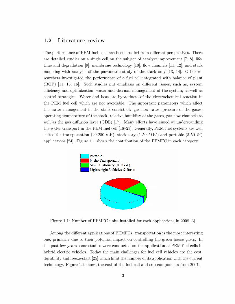
The performance of PEM fuel cells has been studied from different perspectives. Thereare detailed studies on a single cell on the subject of catalyst improvement [7, 8], life-time and degradation [9], membrane technology [10], flow channels [11, 12], and stackmodeling with analysis of the parametric study of the stack only [13, 14]. Other re-searchers investigated the performance of a fuel cell integrated with balance of plant(BOP) [11, 15, 16]. Such studies put emphasis on different issues, such as, systemefficiency and optimization, water and thermal management of the system, as well ascontrol strategies. Water and heat are byproducts of the electrochemical reaction inthe PEM fuel cell which are not avoidable. The important parameters which affectthe water management in the stack consist of: gas flow rates, pressure of the gases,operating temperature of the stack, relative humidity of the gases, gas flow channels aswell as the gas diffusion layer (GDL) [17]. Many efforts have aimed at understandingthe water transport in the PEM fuel cell [18–23]. Generally, PEM fuel systems are wellsuited for transportation (20-250 kW ), stationary (1-50 MW ) and portable (5-50 W )applications [24]. Figure 1.1 shows the contribution of the PEMFC in each category.

Figure 1.1: Number of PEMFC units installed for each applications in 2008 [3].

Among the different applications of PEMFCs, transportation is the most interestingone, primarily due to their potential impact on controlling the green house gases. Inthe past few years some studies were conducted on the application of PEM fuel cells inhybrid electric vehicles. Today the main challenges for fuel cell vehicles are the cost,durability and freeze-start [25] which limit the number of its application with the currenttechnology. Figure 1.2 shows the cost of the fuel cell and sub-components from 2007.

3

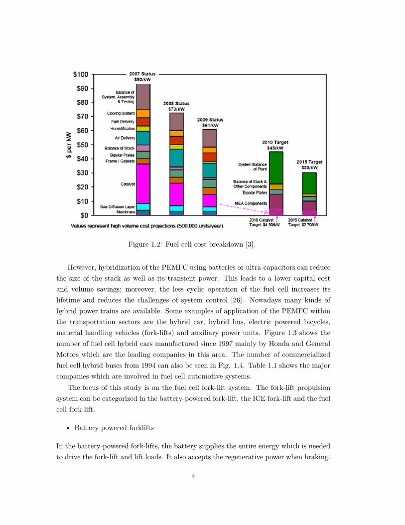
Figure 1.2: Fuel cell cost breakdown [3].

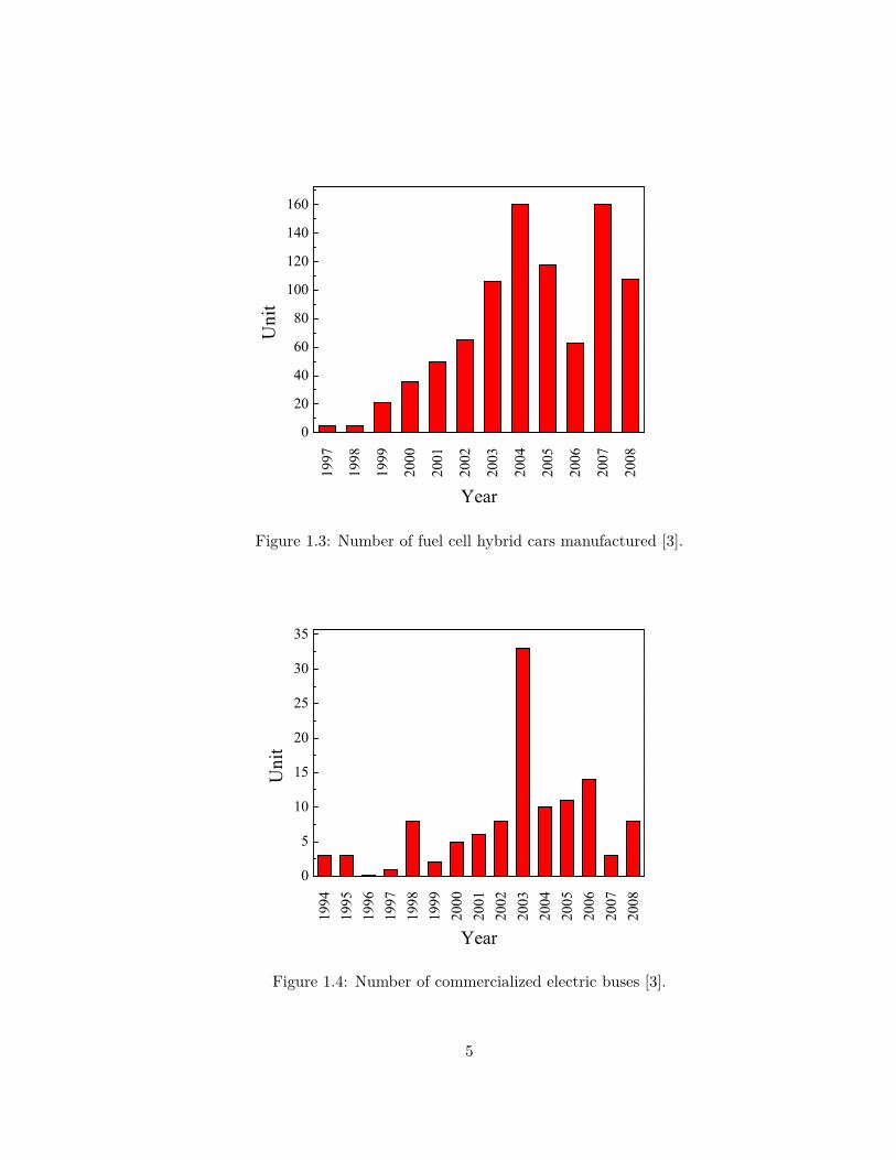
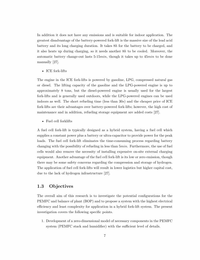
However, hybridization of the PEMFC using batteries or ultra-capacitors can reducethe size of the stack as well as its transient power. This leads to a lower capital costand volume savings; moreover, the less cyclic operation of the fuel cell increases itslifetime and reduces the challenges of system control [26]. Nowadays many kinds ofhybrid power trains are available. Some examples of application of the PEMFC withinthe transportation sectors are the hybrid car, hybrid bus, electric powered bicycles,material handling vehicles (fork-lifts) and auxiliary power units. Figure 1.3 shows thenumber of fuel cell hybrid cars manufactured since 1997 mainly by Honda and GeneralMotors which are the leading companies in this area. The number of commercializedfuel cell hybrid buses from 1994 can also be seen in Fig. 1.4. Table 1.1 shows the majorcompanies which are involved in fuel cell automotive systems.

The focus of this study is on the fuel cell fork-lift system. The fork-lift propulsionsystem can be categorized in the battery-powered fork-lift, the ICE fork-lift and the fuelcell fork-lift.

• Battery powered forklifts

In the battery-powered fork-lifts, the battery supplies the entire energy which is neededto drive the fork-lift and lift loads. It also accepts the regenerative power when braking.

4

1997

1998

1999

2000

2001

2002

2003

2004

2005

2006

2007

2008

0

20

40

60

80

100

120

140

160

Unit

Year

Figure 1.3: Number of fuel cell hybrid cars manufactured [3].

1994

1995

1996

1997

1998

1999

2000

2001

2002

2003

2004

2005

2006

2007

2008

0

5

10

15

20

25

30

35

Unit

Year

Figure 1.4: Number of commercialized electric buses [3].

5

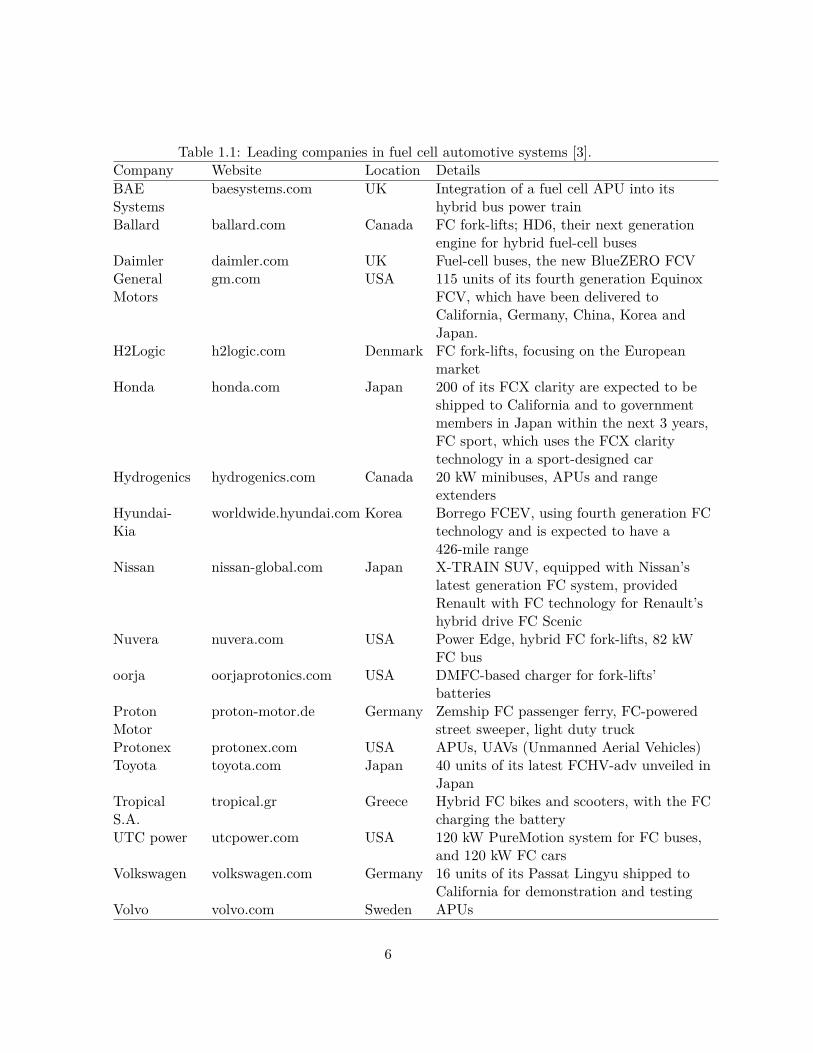
Table 1.1: Leading companies in fuel cell automotive systems [3].Company Website Location DetailsBAESystems

baesystems.com UK Integration of a fuel cell APU into itshybrid bus power train

Ballard ballard.com Canada FC fork-lifts; HD6, their next generationengine for hybrid fuel-cell buses

Daimler daimler.com UK Fuel-cell buses, the new BlueZERO FCVGeneralMotors

gm.com USA 115 units of its fourth generation EquinoxFCV, which have been delivered toCalifornia, Germany, China, Korea andJapan.

H2Logic h2logic.com Denmark FC fork-lifts, focusing on the Europeanmarket

Honda honda.com Japan 200 of its FCX clarity are expected to beshipped to California and to governmentmembers in Japan within the next 3 years,FC sport, which uses the FCX claritytechnology in a sport-designed car

Hydrogenics hydrogenics.com Canada 20 kW minibuses, APUs and rangeextenders

Hyundai-Kia

worldwide.hyundai.com Korea Borrego FCEV, using fourth generation FCtechnology and is expected to have a426-mile range

Nissan nissan-global.com Japan X-TRAIN SUV, equipped with Nissan’slatest generation FC system, providedRenault with FC technology for Renault’shybrid drive FC Scenic

Nuvera nuvera.com USA Power Edge, hybrid FC fork-lifts, 82 kWFC bus

oorja oorjaprotonics.com USA DMFC-based charger for fork-lifts’batteries

ProtonMotor

proton-motor.de Germany Zemship FC passenger ferry, FC-poweredstreet sweeper, light duty truck

Protonex protonex.com USA APUs, UAVs (Unmanned Aerial Vehicles)Toyota toyota.com Japan 40 units of its latest FCHV-adv unveiled in

JapanTropicalS.A.

tropical.gr Greece Hybrid FC bikes and scooters, with the FCcharging the battery

UTC power utcpower.com USA 120 kW PureMotion system for FC buses,and 120 kW FC cars

Volkswagen volkswagen.com Germany 16 units of its Passat Lingyu shipped toCalifornia for demonstration and testing

Volvo volvo.com Sweden APUs

6

In addition it does not have any emissions and is suitable for indoor application. Thegreatest disadvantage of the battery-powered fork-lift is the massive size of the lead acidbattery and its long charging duration. It takes 8h for the battery to be charged, andit also heats up during charging, so it needs another 8h to be cooled. Moreover, theautomatic battery change-out lasts 5-15min, though it takes up to 45min to be donemanually [27].

• ICE fork-lifts

The engine in the ICE fork-lifts is powered by gasoline, LPG, compressed natural gasor diesel. The lifting capacity of the gasoline and the LPG-powered engine is up toapproximately 8 tons, but the diesel-powered engine is usually used for the largestfork-lifts and is generally used outdoors, while the LPG-powered engines can be usedindoors as well. The short refueling time (less than 30s) and the cheaper price of ICEfork-lifts are their advantages over battery-powered fork-lifts; however, the high cost ofmaintenance and in addition, refueling storage equipment are added costs [27].

• Fuel cell forklifts

A fuel cell fork-lift is typically designed as a hybrid system, having a fuel cell whichsupplies a constant power plus a battery or ultra-capacitor to provide power for the peakloads. The fuel cell fork-lift eliminates the time-consuming process regarding batterychanging with the possibility of refueling in less than 5min. Furthermore, the use of fuelcells would also remove the necessity of installing expensive on-site external chargingequipment. Another advantage of the fuel cell fork-lift is its low or zero emission, thoughthere may be some safety concerns regarding the compression and storage of hydrogen.The application of fuel cell fork-lifts will result in lower logistics but higher capital cost,due to the lack of hydrogen infrastructure [27].

1.3 Objectives

The overall aim of this research is to investigate the potential configurations for thePEMFC and balance of plant (BOP) and to propose a system with the highest electricalefficiency and least complexity for application in a hybrid fork-lift system. The presentinvestigation covers the following specific points.

1. Development of a zero-dimensional model of necessary components in the PEMFCsystem (PEMFC stack and humidifier) with the sufficient level of details.

7

2. Construction of a prototype model of the total plant.

3. Improvement of the model based on theory and experiments.

4. Account of the water and thermal management of the system.

5. Design of an ejector for the anode recirculation in the PEMFC system.

6. Application of the PEMFC and BOP in a virtual fork-lift.

1.4 Methodology

The applied methodology can be split into three parts in order to cover the aforemen-tioned topics. Different simulation tools have been used in order to serve the purposein each part.

• The first four parts have been developed by the DNA (Dynamic Network Analysis)program. DNA is an in-house software, which is a FORTRAN-based simulationtool. This code contains various types of heat exchangers, compressors, pumps,etc. that have been developed over many years. The user can easily add newcomponents to the library components, which is also the case for the fuel celland the humidifier in this study. DNA can handle both steady-state and dynamicsimulations. Furthermore, the mass and energy balance is automatically generatedin DNA. The program is free and open source as well. For more information, see[28].

• Part 5 involves a CFD modeling of an ejector for application in fork-lift system.The simulation has been carried out in ANSYS-FLUENT 14.

• Part 6 pointed out the performance of a forklift truck powered by a hybrid systemconsisting of a PEM fuel cell and a lead acid battery. The simulation is run inLFM (Light, Fast, and Modifiable). LFM is a component-based program whichoperates in Matlab/Simulink.

1.5 Thesis outline

The thesis is divided into 7 chapters and 2 appendixes.

Chapter 1 is an introduction to the project containing the study motiva-tion, literature review, objectives, methodology and outline of the thesis.

8

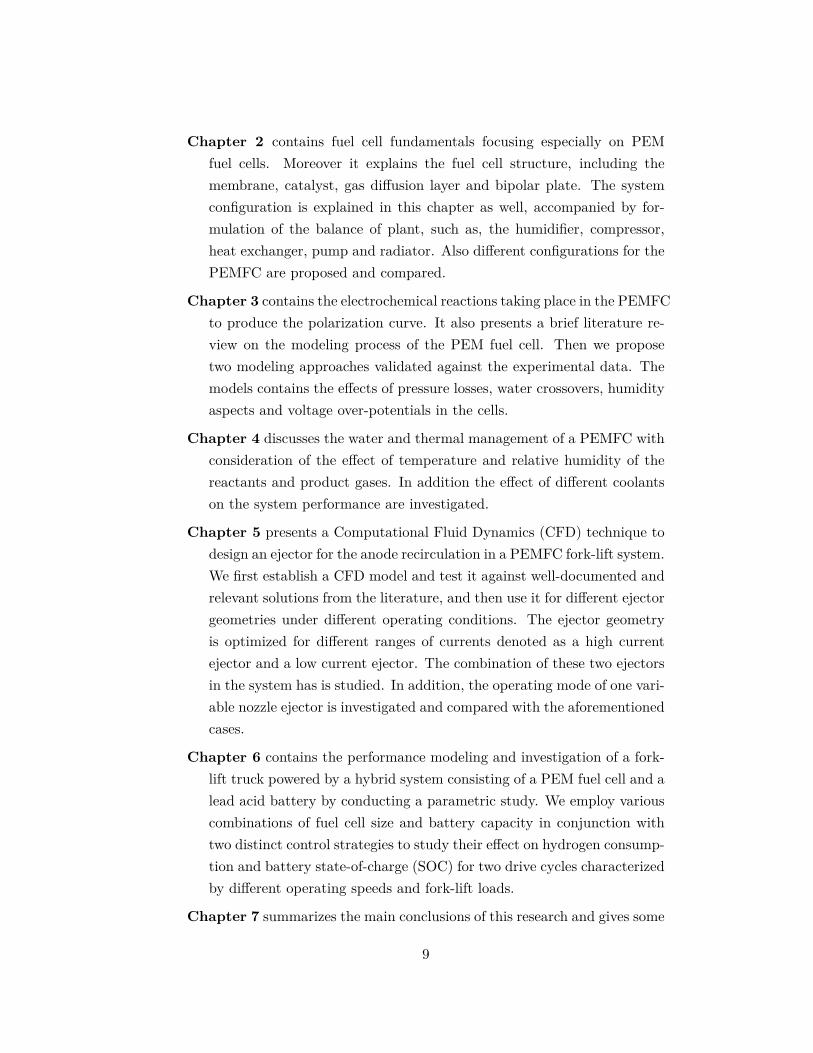
Chapter 2 contains fuel cell fundamentals focusing especially on PEMfuel cells. Moreover it explains the fuel cell structure, including themembrane, catalyst, gas diffusion layer and bipolar plate. The systemconfiguration is explained in this chapter as well, accompanied by for-mulation of the balance of plant, such as, the humidifier, compressor,heat exchanger, pump and radiator. Also different configurations for thePEMFC are proposed and compared.

Chapter 3 contains the electrochemical reactions taking place in the PEMFCto produce the polarization curve. It also presents a brief literature re-view on the modeling process of the PEM fuel cell. Then we proposetwo modeling approaches validated against the experimental data. Themodels contains the effects of pressure losses, water crossovers, humidityaspects and voltage over-potentials in the cells.

Chapter 4 discusses the water and thermal management of a PEMFC withconsideration of the effect of temperature and relative humidity of thereactants and product gases. In addition the effect of different coolantson the system performance are investigated.

Chapter 5 presents a Computational Fluid Dynamics (CFD) technique todesign an ejector for the anode recirculation in a PEMFC fork-lift system.We first establish a CFD model and test it against well-documented andrelevant solutions from the literature, and then use it for different ejectorgeometries under different operating conditions. The ejector geometryis optimized for different ranges of currents denoted as a high currentejector and a low current ejector. The combination of these two ejectorsin the system has is studied. In addition, the operating mode of one vari-able nozzle ejector is investigated and compared with the aforementionedcases.

Chapter 6 contains the performance modeling and investigation of a fork-lift truck powered by a hybrid system consisting of a PEM fuel cell and alead acid battery by conducting a parametric study. We employ variouscombinations of fuel cell size and battery capacity in conjunction withtwo distinct control strategies to study their effect on hydrogen consump-tion and battery state-of-charge (SOC) for two drive cycles characterizedby different operating speeds and fork-lift loads.

Chapter 7 summarizes the main conclusions of this research and gives some

9

recommendations for further work.

Appendix A contains the source code of different components, such as, thehumidifier component model, models of the PEMFC component, a flowsheet of the component models with node numbers, DNA Input as wellas DNA output for the PEMFC system.

Appendixes B-G contains research output in the form of peer-reviewedjournal and conference papers.

10

Chapter 2

System configuration

2.1 Fuel cell fundamentals

A fuel cell is an electrochemical device which converts the chemical energy of the fueldirectly to electricity. A fuel cell is similar to a battery, but unlike the battery, it cangenerate electricity as long as it is fed by the fuel. A fuel cell is composed of differentparts, a negatively-charged electrode (anode), a positively-charged electrode (cathode)and an electrolyte membrane. In a fuel cell hydrogen is oxidized on the anode side,and oxygen is reduced on the cathode side. The electrons pass through the externalcircuit and produce electricity. At the same time, the protons transfer from the anodeto the cathode through an internal circuit, react with oxygen and form water andproduce heat. A catalyst is used in both the anode and cathode sides to speed up theelectrochemical reaction. Figure. 2.1 shows a schematic of a single cell accompanied bythe electrochemical reactions on the anode and cathode sides.

11

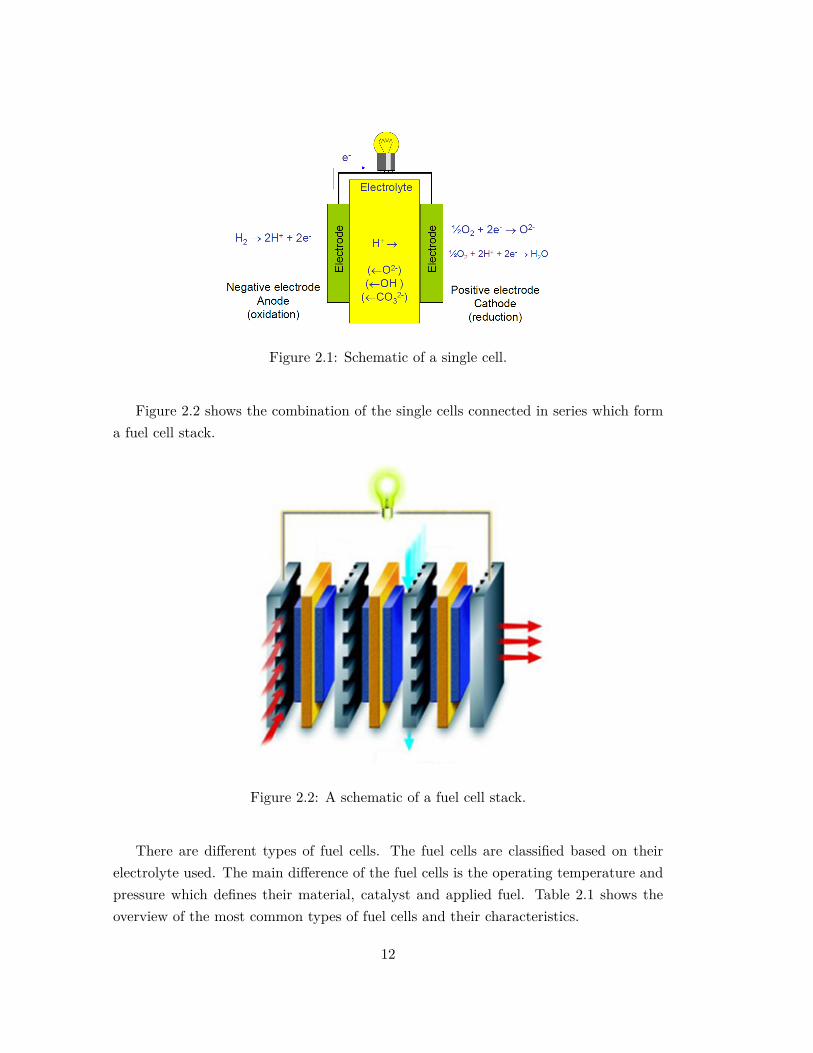
Figure 2.1: Schematic of a single cell.

Figure 2.2 shows the combination of the single cells connected in series which forma fuel cell stack.

Figure 2.2: A schematic of a fuel cell stack.

There are different types of fuel cells. The fuel cells are classified based on theirelectrolyte used. The main difference of the fuel cells is the operating temperature andpressure which defines their material, catalyst and applied fuel. Table 2.1 shows theoverview of the most common types of fuel cells and their characteristics.

12

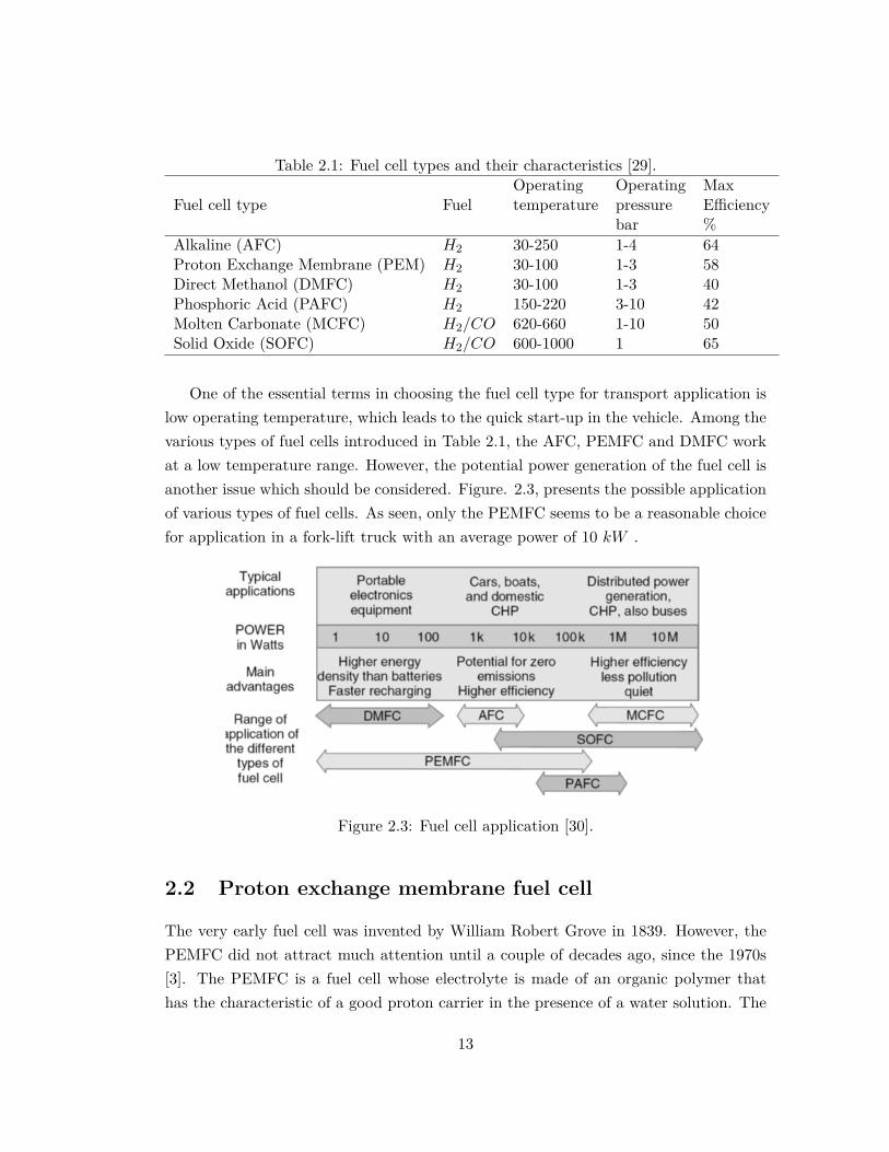
Table 2.1: Fuel cell types and their characteristics [29].

Fuel cell type FuelOperating Operating Maxtemperature pressure Efficiency

bar %Alkaline (AFC) H2 30-250 1-4 64Proton Exchange Membrane (PEM) H2 30-100 1-3 58Direct Methanol (DMFC) H2 30-100 1-3 40Phosphoric Acid (PAFC) H2 150-220 3-10 42Molten Carbonate (MCFC) H2/CO 620-660 1-10 50Solid Oxide (SOFC) H2/CO 600-1000 1 65

One of the essential terms in choosing the fuel cell type for transport application islow operating temperature, which leads to the quick start-up in the vehicle. Among thevarious types of fuel cells introduced in Table 2.1, the AFC, PEMFC and DMFC workat a low temperature range. However, the potential power generation of the fuel cell isanother issue which should be considered. Figure. 2.3, presents the possible applicationof various types of fuel cells. As seen, only the PEMFC seems to be a reasonable choicefor application in a fork-lift truck with an average power of 10 kW .

Figure 2.3: Fuel cell application [30].

2.2 Proton exchange membrane fuel cell

The very early fuel cell was invented by William Robert Grove in 1839. However, thePEMFC did not attract much attention until a couple of decades ago, since the 1970s[3]. The PEMFC is a fuel cell whose electrolyte is made of an organic polymer thathas the characteristic of a good proton carrier in the presence of a water solution. The

13

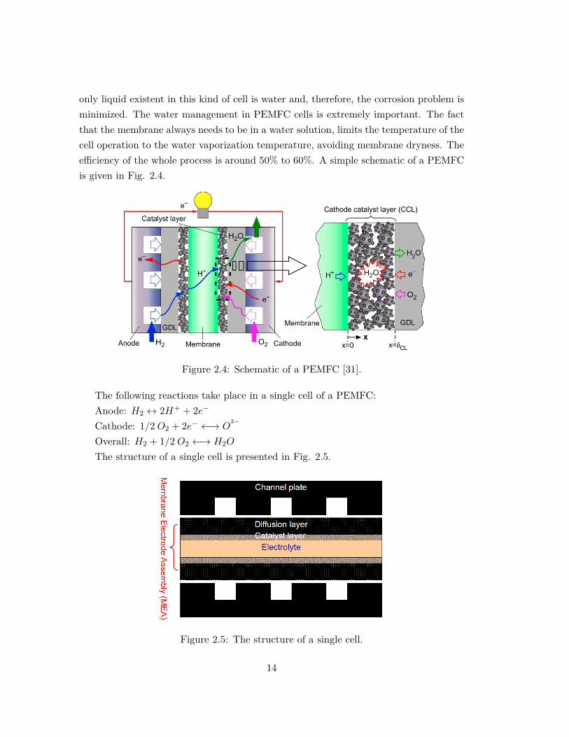
only liquid existent in this kind of cell is water and, therefore, the corrosion problem isminimized. The water management in PEMFC cells is extremely important. The factthat the membrane always needs to be in a water solution, limits the temperature of thecell operation to the water vaporization temperature, avoiding membrane dryness. Theefficiency of the whole process is around 50% to 60%. A simple schematic of a PEMFCis given in Fig. 2.4.

Figure 2.4: Schematic of a PEMFC [31].

The following reactions take place in a single cell of a PEMFC:Anode: H2 ↔ 2H+ + 2e−

Cathode: 1/2O2 + 2e− ←→ O2−

Overall: H2 + 1/2O2 ←→ H2O

The structure of a single cell is presented in Fig. 2.5.

Figure 2.5: The structure of a single cell.

14

2.2.1 Membrane

Depending on the type of the fuel cell, the membrane can be liquid or solid but theprincipal function is the same, that is, to transport protons generated at the anode tothe cathode side where they react with oxygen to produce water. The electrolyte alsofunctions as an electron separator. During the oxidation and reduction processes, theelectron released must not be allowed to pass directly through the electrolyte. If theelectrons pass directly through the electrolyte, a short circuit of the cell will occur andthe fuel cell will fail. General demands for a good membrane are:

• High specific ionic conductivity (S/cm)• Low reactant permeability• High electronic resistivity (Ωcm) - electronic insulatorThe most typical electrolyte used in a low temperature PEMFC is a fully fluorinated

Teflon-based material (perfluoro sulfonic acid [PFSA]) with the generic brand name,Nafion. Nafion 117 is the most common one [29].

2.2.2 Catalyst

Catalyst layers are found on the anode side of the membrane as well as the cathode side.The catalyst layers speed up the electrochemical reaction on the anode and the cathodeside. The catalyst layer typically consists of platinum supported by carbon structuresand is applied directly to the membrane surface. General demands for a good catalystare as follows:

• High intrinsic activity (high i0 on the true surface)• Large surface areas• Good contact to current collector, gases and electrolyte (three-phase area)• Tolerant towards impurities (e.g. CO, sulphur, Cl−)• Low sintering rate• High corrosion resistance

2.2.3 Gas diffusion layer (GDL)

The catalyst layers together with the membrane make up the membrane electrode as-sembly (MEA). The GDL is a carbon-fiber paper gas diffusion layer in which the MEAis sandwiched. The GDL serves two main purposes. One is to transport reactant gasesfrom the gas supply channels to the reaction site, and the other one is to transfer pro-duced water from the reaction site in to the bipolar plates where it can be removedfrom the cell.

15

2.2.4 Bipolar plate

The bipolar plate is the outer structure of the PEMFC. The plates are made of alight-weight, strong, gas-impermeable, and electron-conducting material. In most ofthe PEMFC, graphite or other non-corrosive materials with high conductivity and rigidstructure can be used [29]. The main purpose of the bipolar plate is to serve as the gassupply from the source to the reaction sites by a series of serpentine flow field networks.The bipolar plate also acts as a current collector.

2.3 Overall system design

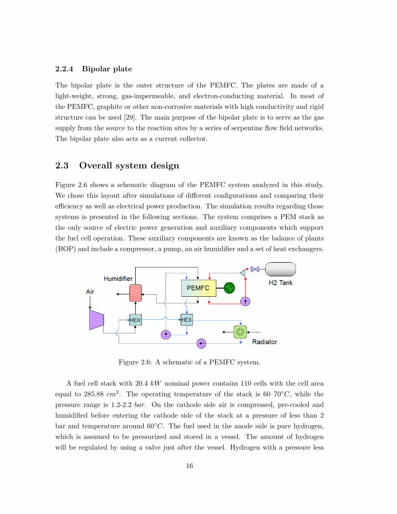
Figure 2.6 shows a schematic diagram of the PEMFC system analyzed in this study.We chose this layout after simulations of different configurations and comparing theirefficiency as well as electrical power production. The simulation results regarding thosesystems is presented in the following sections. The system comprises a PEM stack asthe only source of electric power generation and auxiliary components which supportthe fuel cell operation. These auxiliary components are known as the balance of plants(BOP) and include a compressor, a pump, an air humidifier and a set of heat exchangers.

Figure 2.6: A schematic of a PEMFC system.

A fuel cell stack with 20.4 kW nominal power contains 110 cells with the cell areaequal to 285.88 cm2. The operating temperature of the stack is 60–70C, while thepressure range is 1.2-2.2 bar. On the cathode side air is compressed, pre-cooled andhumidified before entering the cathode side of the stack at a pressure of less than 2bar and temperature around 60C. The fuel used in the anode side is pure hydrogen,which is assumed to be pressurized and stored in a vessel. The amount of hydrogenwill be regulated by using a valve just after the vessel. Hydrogen with a pressure less

16

than 2.2 bar and temperature around 48C enters the anode side of the stack. Sinceall the fuel cannot react inside the stack, then the rest is collected and sent back to theanode stream via a recirculation pump. To prevent dehydration in the membrane, airand fuel must be humidified. In the air side there is a humidifier which uses some of thewater from the cathode outlet to humidify the inlet air. The relative humidity of the airprior to the stack is set to 95% in the calculations; although other values can be chosen.On the fuel side there is no humidifier, and the fuel can reach the desired humidity bymeans of the water cross-over effect through the membrane from the cathode to theanode. Depending on the stack power output, the anode inlet humidity is between 78%to 100%. This aspect is revisited later in this study. For thermal management twoseparate cooling circuits are used, denoted as inner and outer loops. The inner loop isused for stack cooling, and the coolant keeps the stack temperature around 70C. Therejected heat from the stack via the coolant in the inner loop is dedicated to the coolantin the outer loop with different working temperatures around 25-60C, and the wasteheat in the outer loop is rejected through a radiator. Another possible alternative forcooling the system is using one cooling circuit instead of two. In this way one heatexchanger can be illuminated, and the coolant can be circulated through one ratherlarger heat exchanger and can cool down the stack. But the fact is that, the inlet andthe outlet temperature of the coolant for the stack should be equal to the reactant andthe product gas temperature, respectively, for the best operation of the stack. Withone cooling circuit it is almost impossible to predefine the inlet temperature of thecoolant entering the stack, since the coolant is going through different components.But the advantage of two cooling circuits over one is that the coolant temperature ismore flexible, and it is very easy to regulate it against the variation of the stack andthe air temperature. For this reason this configuration has been chosen. Beside thesystem configurations, we apply different coolants with various temperature range inthe system, and we elaborate on their behavior in this study. The DNA program is usedfor the model development of the fuel cell and the BOP. The details of the programwere presented in Chapter 1. The following sections provide the details of the BOP,while the modeling approach of the PEMFC is explained in the next chapter.

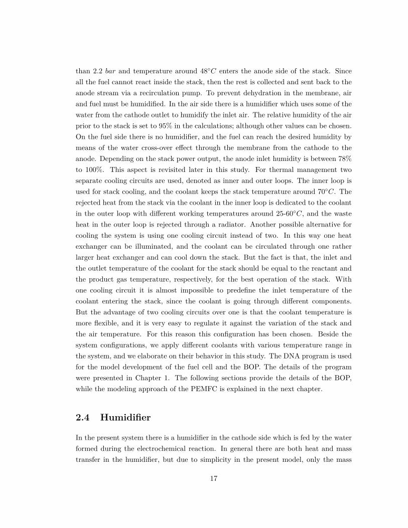
2.4 Humidifier

In the present system there is a humidifier in the cathode side which is fed by the waterformed during the electrochemical reaction. In general there are both heat and masstransfer in the humidifier, but due to simplicity in the present model, only the mass

17

balance is considered, and the inlet and the outlet temperature of the humidifier aredefined by the experimental set up with the same operating conditions as the model. Inother words, the humidifier is acting like a mixer in which dry air enters and dependson the inlet temperature of the stack, required amount of water is added to it in orderto reach to the desired level of humidity, which is 95% in most cases. But it may bechanged to the other values as well. A schematic of the humidifier can be seen in Fig.2.7.

Figure 2.7: A schematic of the humidifier.

The relative humidity, (RH) can be defined as the ratio of partial pressure of thevapor, Pv, to partial pressure of that in the saturated mixture, Pg, at the same temper-ature:

RH = PvPg

(2.1)

where Pg can be evaluated via the following equation:

Pg = 2.609× 10−11.T 5out + 3.143× 10−9.T 4

out + 2.308× 10−7.T 3out

+1.599× 10−5.T 2out + 4.11× 10−4.Tout + 6.332× 10−3 (2.2)

Tout represents the outlet temperature of the humidifier as well as the stack inlettemperature. The humidity ratio, φ, is the mass flow of the water vapor, mv, to themass flow of the dry fluid, mda, which is air in this case. It can be expressed by:

φ = mv

mda(2.3)

By assuming the gases are ideal, the humidity ratio can be correlated to the partialpressures and molecular weights:

18

mv = Pv.V

Rv.T= Pv.V .Mv

R.T(2.4)

mda = Pa.V

Ra.T= Pa.V .Ma

R.T(2.5)

By inserting of equations (2.4-2.5) in equation 2.3 the following expression is obtainedfor the humidity ratio:

φ = Mv.PvMa.Pa

(2.6)

which in the case of the air-water mixture it becomes:

φ = 0.622PvPa

(2.7)

By assuming the requested relative humidity at the cathode inlet and applying this setof equations, the amount of water which is needed for humidification can be simplycalculated via the mass balance equation.

mda,in + mv,in1 + mv,in2 = mda,out + mv,out (2.8)

2.5 Compressor

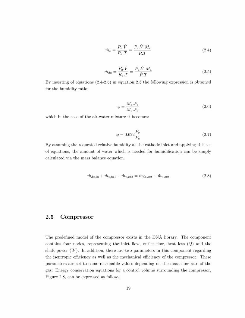
The predefined model of the compressor exists in the DNA library. The componentcontains four nodes, representing the inlet flow, outlet flow, heat loss (Q) and theshaft power (W ). In addition, there are two parameters in this component regardingthe isentropic efficiency as well as the mechanical efficiency of the compressor. Theseparameters are set to some reasonable values depending on the mass flow rate of thegas. Energy conservation equations for a control volume surrounding the compressor,Figure 2.8, can be expressed as follows:

19

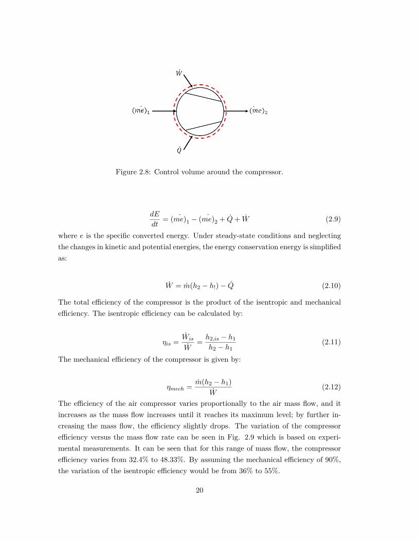
Figure 2.8: Control volume around the compressor.

dE

dt= (me)1 − (me)2 + Q+ W (2.9)

where e is the specific converted energy. Under steady-state conditions and neglectingthe changes in kinetic and potential energies, the energy conservation energy is simplifiedas:

W = m(h2 − h!)− Q (2.10)

The total efficiency of the compressor is the product of the isentropic and mechanicalefficiency. The isentropic efficiency can be calculated by:

ηis = Wis

W= h2,is − h1

h2 − h1(2.11)

The mechanical efficiency of the compressor is given by:

ηmech = m(h2 − h1)W

(2.12)

The efficiency of the air compressor varies proportionally to the air mass flow, and itincreases as the mass flow increases until it reaches its maximum level; by further in-creasing the mass flow, the efficiency slightly drops. The variation of the compressorefficiency versus the mass flow rate can be seen in Fig. 2.9 which is based on experi-mental measurements. It can be seen that for this range of mass flow, the compressorefficiency varies from 32.4% to 48.33%. By assuming the mechanical efficiency of 90%,the variation of the isentropic efficiency would be from 36% to 55%.

20

0.000 0.005 0.010 0.015 0.020 0.025

35

40

45

50

55

Isen

tropi

c ef

ficie

ncy

[%]

Mass flow rate [kg/s]

Figure 2.9: Variation of isentropic efficiency of the air compressor versus mass flow.

2.6 Heat exchanger

There are different types of heat exchangers in the DNA library. The model used in thisstudy contains five nodes, the hot fluid inlet, the hot fluid outlet, the cold fluid inlet,the cold fluid outlet and the heat loss followed by two parameters. The parameters arepressure loss in the hot fluid side and that in the cold fluid side. The heat exchangermodel is steady state, and the mass flow rate of each fluid is constant. The outer surfaceof the heat exchanger is considered to be perfectly insolated so that the heat loss tothe surrounding can be neglected. Under these assumptions and simplifications, andaccording to the first law of thermodynamics, the rate of heat transfer from the hotfluid must be equal to that of the cold fluid.

Q = mCp,c(Tc,out − Tc,in) (2.13)

Q = mhCp,h(Th,in − Th,out) (2.14)

where Cp is the specific heat capacity, and the subscripts c and h denote the cold andhot fluids, respectively. The pressure drop in the heat exchangers (both on the cold andthe hot side) is assumed to be 50 (mbar).

2.7 Pump

The predefined liquid pump with three nodes, the liquid inlet, the liquid outlet andthe shaft power exist in the DNA library. The only parameter for this component is

21

the pump efficiency which is set to 70% in calculations. This issue is elaborated in thefollowing sections. We calculate the power consumption of the pump as:

W = mv1(P2 − P1) (2.15)

where v1 is the specific volume of the fluid at the pump entrance.

2.8 Radiator

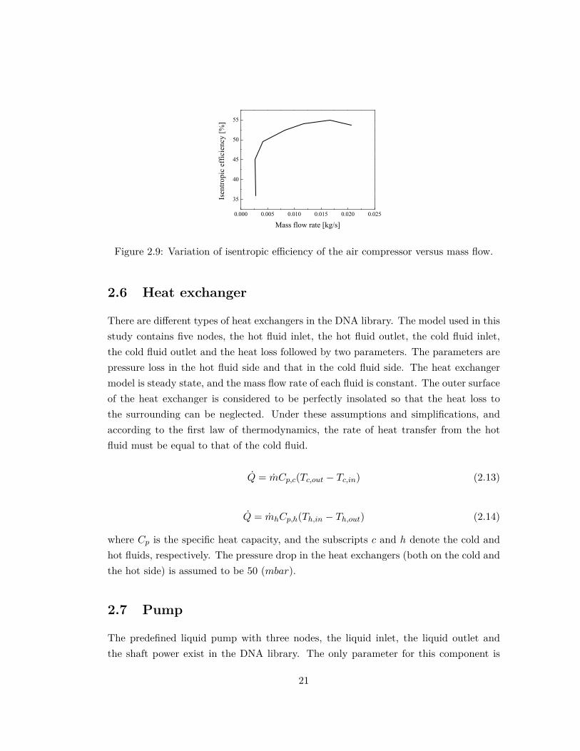
Since there is no predefined model for the radiator in DNA, it is established by com-bining two components, an air compressor and a heat exchanger. The assumed modelof the radiator is shown in Fig. 2.10. As seen, the air flows to the cold side through acompressor. The compression pressure of the air is defined so that the power consump-tion of the compressor is equal to the power consumption of the fan. The hot coolant,mcoolant, passes through a heat exchanger where it can exchange the heat with the airflow on the cold side.

Figure 2.10: A schematic of the radiator.

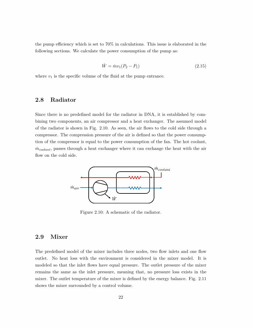
2.9 Mixer

The predefined model of the mixer includes three nodes, two flow inlets and one flowoutlet. No heat loss with the environment is considered in the mixer model. It ismodeled so that the inlet flows have equal pressure. The outlet pressure of the mixerremains the same as the inlet pressure, meaning that, no pressure loss exists in themixer. The outlet temperature of the mixer is defined by the energy balance. Fig. 2.11shows the mixer surrounded by a control volume.

22

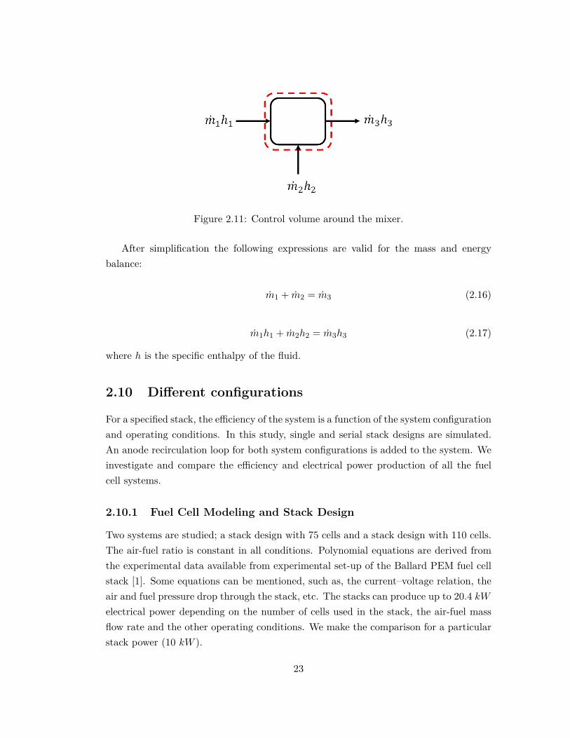
Figure 2.11: Control volume around the mixer.

After simplification the following expressions are valid for the mass and energybalance:

m1 + m2 = m3 (2.16)

m1h1 + m2h2 = m3h3 (2.17)

where h is the specific enthalpy of the fluid.

2.10 Different configurations

For a specified stack, the efficiency of the system is a function of the system configurationand operating conditions. In this study, single and serial stack designs are simulated.An anode recirculation loop for both system configurations is added to the system. Weinvestigate and compare the efficiency and electrical power production of all the fuelcell systems.

2.10.1 Fuel Cell Modeling and Stack Design

Two systems are studied; a stack design with 75 cells and a stack design with 110 cells.The air-fuel ratio is constant in all conditions. Polynomial equations are derived fromthe experimental data available from experimental set-up of the Ballard PEM fuel cellstack [1]. Some equations can be mentioned, such as, the current–voltage relation, theair and fuel pressure drop through the stack, etc. The stacks can produce up to 20.4 kWelectrical power depending on the number of cells used in the stack, the air-fuel massflow rate and the other operating conditions. We make the comparison for a particularstack power (10 kW ).

23

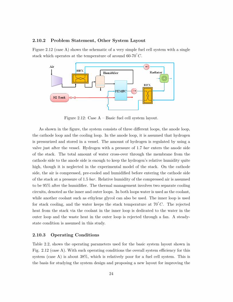
2.10.2 Problem Statement, Other System Layout

Figure 2.12 (case A) shows the schematic of a very simple fuel cell system with a singlestack which operates at the temperature of around 60-70

C.

Figure 2.12: Case A – Basic fuel cell system layout.

As shown in the figure, the system consists of three different loops, the anode loop,the cathode loop and the cooling loop. In the anode loop, it is assumed that hydrogenis pressurized and stored in a vessel. The amount of hydrogen is regulated by using avalve just after the vessel. Hydrogen with a pressure of 1.7 bar enters the anode sideof the stack. The total amount of water cross-over through the membrane from thecathode side to the anode side is enough to keep the hydrogen’s relative humidity quitehigh, though it is neglected in the experimental model of the stack. On the cathodeside, the air is compressed, pre-cooled and humidified before entering the cathode sideof the stack at a pressure of 1.5 bar. Relative humidity of the compressed air is assumedto be 95% after the humidifier. The thermal management involves two separate coolingcircuits, denoted as the inner and outer loops. In both loops water is used as the coolant,while another coolant such as ethylene glycol can also be used. The inner loop is usedfor stack cooling, and the water keeps the stack temperature at 70

C. The rejectedheat from the stack via the coolant in the inner loop is dedicated to the water in theouter loop and the waste heat in the outer loop is rejected through a fan. A steady-state condition is assumed in this study.

2.10.3 Operating Conditions

Table 2.2, shows the operating parameters used for the basic system layout shown inFig. 2.12 (case A). With such operating conditions the overall system efficiency for thissystem (case A) is about 38%, which is relatively poor for a fuel cell system. This isthe basis for studying the system design and proposing a new layout for improving the

24

system efficiency. In the following sections, we suggest new suggested system layoutsand show that it is possible to increase the system efficiency considerably.

Table 2.2: Operating conditions, (case A).Parameter DescriptionAir inlet pressure to stack 1.5 barAir inlet temperature to stack 60

CHydrogen inlet pressure to stack 1.7 barHydrogen inlet temperature to stack 60

CCoolant mass flow rate of inner loop 0.4 kg/sCoolant pressure of inner loop 1.4 barCoolant temperature of inner loop 58

CCoolant mass flow rate of outer loop 0.28 kg/sCoolant pressure of outer loop 1.4 barCoolant temperature of outer loop 50

C

2.10.4 Other Suggested System Layouts

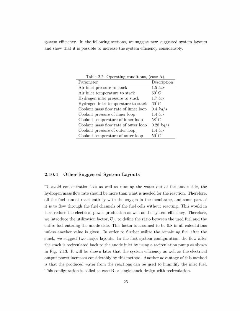
To avoid concentration loss as well as running the water out of the anode side, thehydrogen mass flow rate should be more than what is needed for the reaction. Therefore,all the fuel cannot react entirely with the oxygen in the membrane, and some part ofit is to flow through the fuel channels of the fuel cells without reacting. This would inturn reduce the electrical power production as well as the system efficiency. Therefore,we introduce the utilization factor, Uf , to define the ratio between the used fuel and theentire fuel entering the anode side. This factor is assumed to be 0.8 in all calculationsunless another value is given. In order to further utilize the remaining fuel after thestack, we suggest two major layouts. In the first system configuration, the flow afterthe stack is recirculated back to the anode inlet by using a recirculation pump as shownin Fig. 2.13. It will be shown later that the system efficiency as well as the electricaloutput power increases considerably by this method. Another advantage of this methodis that the produced water from the reactions can be used to humidify the inlet fuel.This configuration is called as case B or single stack design with recirculation.

25

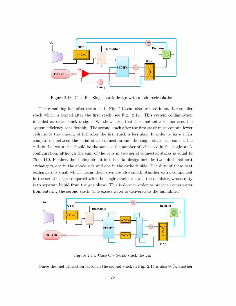
Figure 2.13: Case B – Single stack design with anode recirculation.

The remaining fuel after the stack in Fig. 2.12 can also be used in another smallerstack which is placed after the first stack; see Fig. 2.14. This system configurationis called as serial stack design. We show later that this method also increases thesystem efficiency considerably. The second stack after the first stack must contain fewercells, since the amount of fuel after the first stack is less also. In order to have a faircomparison between the serial stack connection and the single stack, the sum of thecells in the two stacks should be the same as the number of cells used in the single stackconfiguration; although the sum of the cells in two serial connected stacks is equal to75 or 110. Further, the cooling circuit in this serial design includes two additional heatexchangers, one in the anode side and one in the cathode side. The duty of these heatexchangers is small which means their sizes are also small. Another extra componentin the serial design compared with the single stack design is the demister, whose dutyis to separate liquid from the gas phase. This is done in order to prevent excess waterfrom entering the second stack. The excess water is delivered to the humidifier.

Figure 2.14: Case C – Serial stack design.

Since the fuel utilization factor in the second stack in Fig. 2.14 is also 80%, another

26

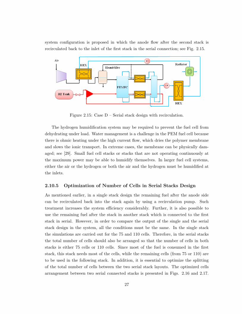
system configuration is proposed in which the anode flow after the second stack isrecirculated back to the inlet of the first stack in the serial connection; see Fig. 2.15.

Figure 2.15: Case D – Serial stack design with recirculation.

The hydrogen humidification system may be required to prevent the fuel cell fromdehydrating under load. Water management is a challenge in the PEM fuel cell becausethere is ohmic heating under the high current flow, which dries the polymer membraneand slows the ionic transport. In extreme cases, the membrane can be physically dam-aged; see [29]. Small fuel cell stacks or stacks that are not operating continuously atthe maximum power may be able to humidify themselves. In larger fuel cell systems,either the air or the hydrogen or both the air and the hydrogen must be humidified atthe inlets.

2.10.5 Optimization of Number of Cells in Serial Stacks Design

As mentioned earlier, in a single stack design the remaining fuel after the anode sidecan be recirculated back into the stack again by using a recirculation pump. Suchtreatment increases the system efficiency considerably. Further, it is also possible touse the remaining fuel after the stack in another stack which is connected to the firststack in serial. However, in order to compare the output of the single and the serialstack design in the system, all the conditions must be the same. In the single stackthe simulations are carried out for the 75 and 110 cells. Therefore, in the serial stacksthe total number of cells should also be arranged so that the number of cells in bothstacks is either 75 cells or 110 cells. Since most of the fuel is consumed in the firststack, this stack needs most of the cells, while the remaining cells (from 75 or 110) areto be used in the following stack. In addition, it is essential to optimize the splittingof the total number of cells between the two serial stack layouts. The optimized cellsarrangement between two serial connected stacks is presented in Figs. 2.16 and 2.17.

27

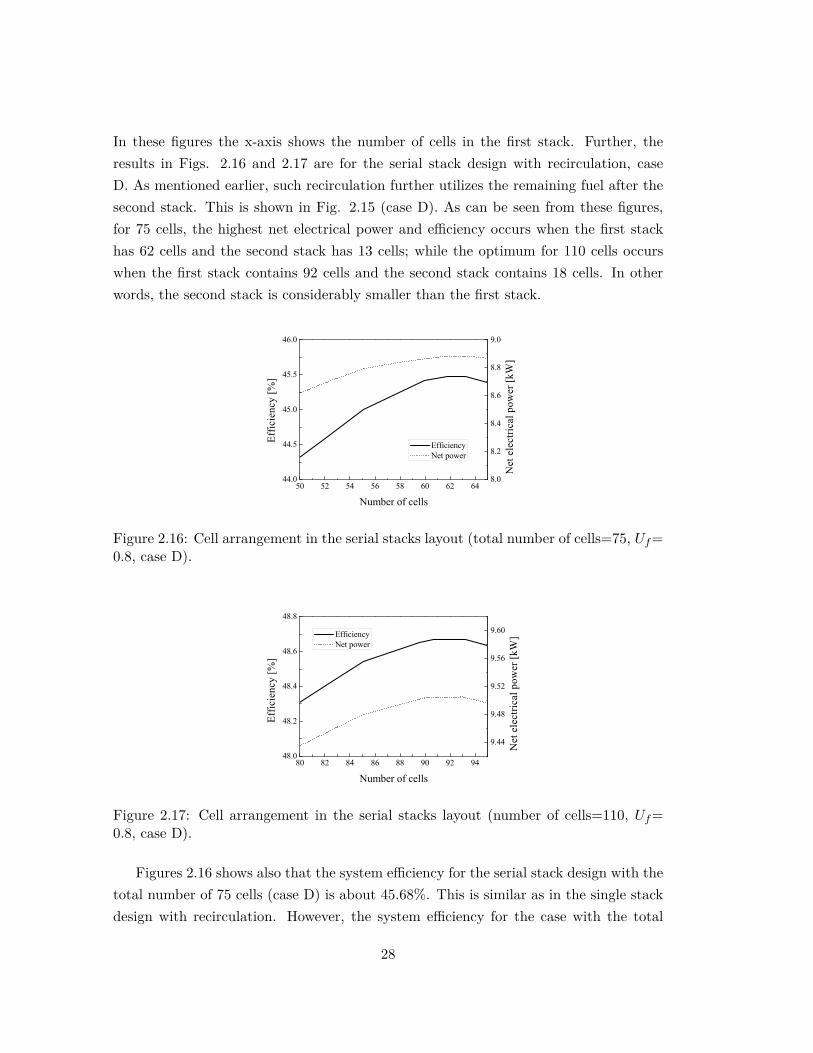
In these figures the x-axis shows the number of cells in the first stack. Further, theresults in Figs. 2.16 and 2.17 are for the serial stack design with recirculation, caseD. As mentioned earlier, such recirculation further utilizes the remaining fuel after thesecond stack. This is shown in Fig. 2.15 (case D). As can be seen from these figures,for 75 cells, the highest net electrical power and efficiency occurs when the first stackhas 62 cells and the second stack has 13 cells; while the optimum for 110 cells occurswhen the first stack contains 92 cells and the second stack contains 18 cells. In otherwords, the second stack is considerably smaller than the first stack.

50 52 54 56 58 60 62 6444.0

44.5

45.0

45.5

46.0

Efficiency Net power

Number of cells

Effic

ienc

y [%

]

8.0

8.2

8.4

8.6

8.8

9.0

Net

ele

ctric

al p

ower

[kW

]

Figure 2.16: Cell arrangement in the serial stacks layout (total number of cells=75, Uf=0.8, case D).

80 82 84 86 88 90 92 9448.0

48.2

48.4

48.6

48.8

Efficiency Net power

Number of cells

Effic

ienc

y [%

]

9.44

9.48

9.52

9.56

9.60

Net

ele

ctric

al p

ower

[kW

]

Figure 2.17: Cell arrangement in the serial stacks layout (number of cells=110, Uf=0.8, case D).

Figures 2.16 shows also that the system efficiency for the serial stack design with thetotal number of 75 cells (case D) is about 45.68%. This is similar as in the single stackdesign with recirculation. However, the system efficiency for the case with the total

28

number of 110 cells has an efficiency of about 48.7%, which is slightly lower than thesingle stack design with recirculation. In the serial stack design without recirculation(case C), the system efficiency is about 44.0% and 47.0% for 75 and 110 total numberof cells, respectively. For this case, the system efficiency is slightly lower than for thesingle stack with recirculation and the serial stack design with recirculation (case B andcase D).

2.10.6 Case study comparisons

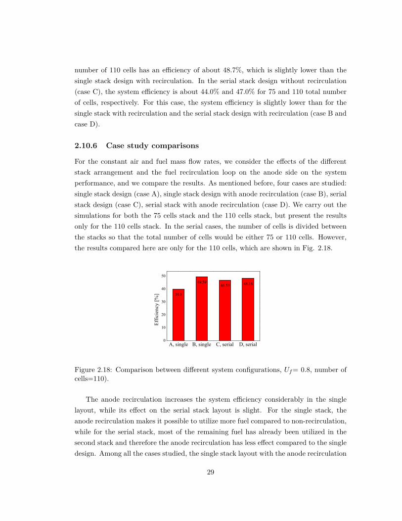
For the constant air and fuel mass flow rates, we consider the effects of the differentstack arrangement and the fuel recirculation loop on the anode side on the systemperformance, and we compare the results. As mentioned before, four cases are studied:single stack design (case A), single stack design with anode recirculation (case B), serialstack design (case C), serial stack with anode recirculation (case D). We carry out thesimulations for both the 75 cells stack and the 110 cells stack, but present the resultsonly for the 110 cells stack. In the serial cases, the number of cells is divided betweenthe stacks so that the total number of cells would be either 75 or 110 cells. However,the results compared here are only for the 110 cells, which are shown in Fig. 2.18.

A, single B, single C, serial D, serial0

10

20

30

40

50

48.1646.5949.59

39.8

Effic

ienc

y [%

]

Figure 2.18: Comparison between different system configurations, Uf= 0.8, number ofcells=110).

The anode recirculation increases the system efficiency considerably in the singlelayout, while its effect on the serial stack layout is slight. For the single stack, theanode recirculation makes it possible to utilize more fuel compared to non-recirculation,while for the serial stack, most of the remaining fuel has already been utilized in thesecond stack and therefore the anode recirculation has less effect compared to the singledesign. Among all the cases studied, the single stack layout with the anode recirculation

29

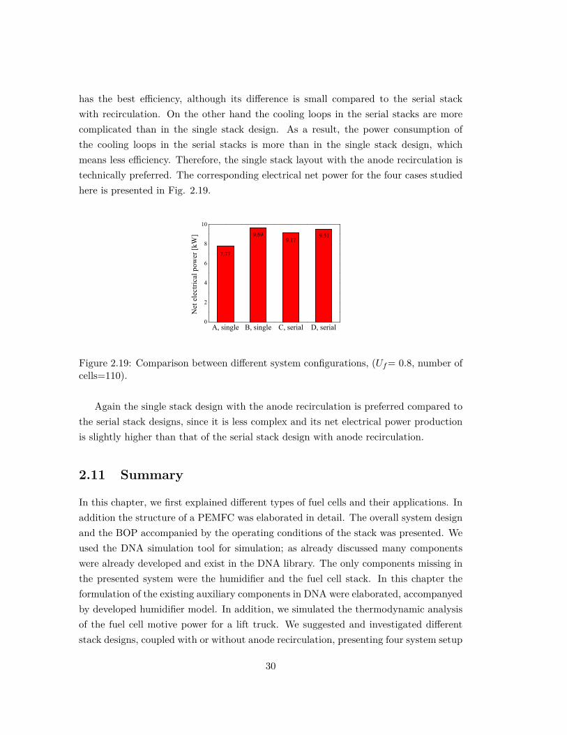
has the best efficiency, although its difference is small compared to the serial stackwith recirculation. On the other hand the cooling loops in the serial stacks are morecomplicated than in the single stack design. As a result, the power consumption ofthe cooling loops in the serial stacks is more than in the single stack design, whichmeans less efficiency. Therefore, the single stack layout with the anode recirculation istechnically preferred. The corresponding electrical net power for the four cases studiedhere is presented in Fig. 2.19.

A, single B, single C, serial D, serial0

2

4

6

8

10

9.519.17

9.69

7.77

Net

ele

ctric

al p

ower

[kW

]

Figure 2.19: Comparison between different system configurations, (Uf= 0.8, number ofcells=110).

Again the single stack design with the anode recirculation is preferred compared tothe serial stack designs, since it is less complex and its net electrical power productionis slightly higher than that of the serial stack design with anode recirculation.

2.11 Summary

In this chapter, we first explained different types of fuel cells and their applications. Inaddition the structure of a PEMFC was elaborated in detail. The overall system designand the BOP accompanied by the operating conditions of the stack was presented. Weused the DNA simulation tool for simulation; as already discussed many componentswere already developed and exist in the DNA library. The only components missing inthe presented system were the humidifier and the fuel cell stack. In this chapter theformulation of the existing auxiliary components in DNA were elaborated, accompanyedby developed humidifier model. In addition, we simulated the thermodynamic analysisof the fuel cell motive power for a lift truck. We suggested and investigated differentstack designs, coupled with or without anode recirculation, presenting four system setup

30

configurations. These are listed as single stack without recirculation (case A), singlestack with recirculation (case B), serial stack without recirculation (case C) and serialstack with recirculation (case D). The calculations were carried out for two sets of cellnumbers, which are equal to 75 and 110 cells. For the 75 cells the efficiency in the basiccase (case A) is 34%, which is quite low. Various approaches for efficiency improvementwere studied to reach system efficiencies of about 50%. The results show that the anoderecirculation loop increases the efficiency in both the single and the serial stack design,but its effect is much larger in the single stack compared to the serial stack design. Forthe 110 cells, there is efficiency improvement due to the anode recirculation; it is about10% for the single stack compared to about 2% in the serial stack design. Another issuediscussed in this study is cell arrangement. We found that without the recirculationloop, the serial stack design has a higher efficiency compared with the single stack,around 7% higher. However, for the systems with anode recirculation, (case B and caseD) the efficiency of the single stack design is about 1% higher than the serial stacklayout. Therefore, the single stack with recirculation (case B) is proposed as the mostefficient fuel cell system because of its high efficiency and simplicity. The developmentof the PEMFC model based on analytical and semi-empirical expression is presented inthe next chapter.

31

Chapter 3

Modeling approach

3.1 Overview

To investigate a PEMFC system (a PEMFC accompanied by the BOP), as mentioned inthe previous chapters, a comprehensive model of the PEMFC and humidifier has beendeveloped. According to the literature the PEMFC models can be based on analyti-cal, semi-empirical and numerical methods. In the current study, a zero-dimensional,steady-state PEMFC model has been developed for application in a 10 kW fork-lifttruck power system, which is based on an older product from H2Logic Company [32].The BOP (Balance of Plant) comprises a compressor, an air humidifier, a set of heatexchangers and a recirculation pump. The model takes into account the effects of pres-sure losses, water crossovers, humidity aspects and voltage over-potentials in the cells.The presented polarization curve for the stack captures the experimental data very well.This model can represent the behavior of various PEM stacks regardless of the dimen-sions if the adjusting parameters are changed accordingly. We discuss several issueshere, namely, the stack operating conditions, thermodynamic efficiency of the systemas well as electrical power.

The developed PEMFC model calculates cell current and mass flow rate of eachspecies at the inlet and outlet of the fuel cell. The calculations are based on the stackpower production as well as on the operating temperature of the PEMFC. Some ofthe the input values are given directly to the PEMFC model, such as, the air and thefuel stoichiometry, operating temperature of the stack, relative humidity at the cathodeinlet, number of cells, inlet pressure as well as pressure drop at the anode and cathode

32

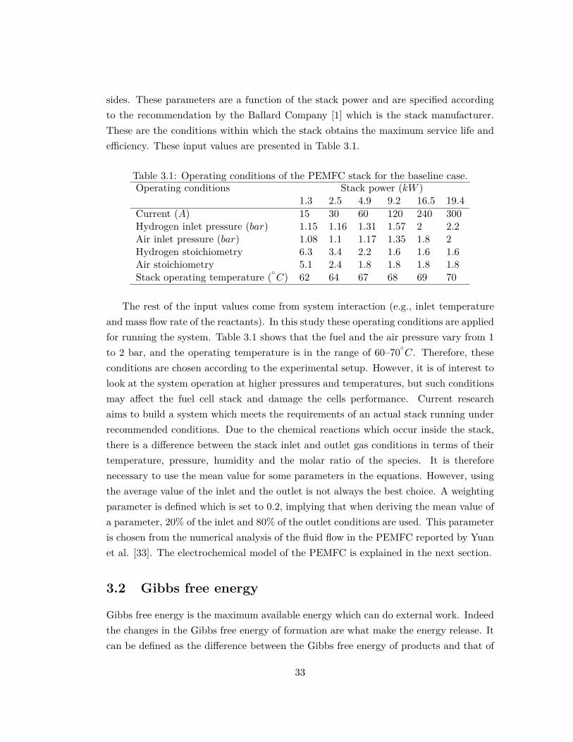
sides. These parameters are a function of the stack power and are specified accordingto the recommendation by the Ballard Company [1] which is the stack manufacturer.These are the conditions within which the stack obtains the maximum service life andefficiency. These input values are presented in Table 3.1.

Table 3.1: Operating conditions of the PEMFC stack for the baseline case.Operating conditions Stack power (kW )

1.3 2.5 4.9 9.2 16.5 19.4Current (A) 15 30 60 120 240 300Hydrogen inlet pressure (bar) 1.15 1.16 1.31 1.57 2 2.2Air inlet pressure (bar) 1.08 1.1 1.17 1.35 1.8 2Hydrogen stoichiometry 6.3 3.4 2.2 1.6 1.6 1.6Air stoichiometry 5.1 2.4 1.8 1.8 1.8 1.8Stack operating temperature (

C) 62 64 67 68 69 70

The rest of the input values come from system interaction (e.g., inlet temperatureand mass flow rate of the reactants). In this study these operating conditions are appliedfor running the system. Table 3.1 shows that the fuel and the air pressure vary from 1to 2 bar, and the operating temperature is in the range of 60–70

C. Therefore, theseconditions are chosen according to the experimental setup. However, it is of interest tolook at the system operation at higher pressures and temperatures, but such conditionsmay affect the fuel cell stack and damage the cells performance. Current researchaims to build a system which meets the requirements of an actual stack running underrecommended conditions. Due to the chemical reactions which occur inside the stack,there is a difference between the stack inlet and outlet gas conditions in terms of theirtemperature, pressure, humidity and the molar ratio of the species. It is thereforenecessary to use the mean value for some parameters in the equations. However, usingthe average value of the inlet and the outlet is not always the best choice. A weightingparameter is defined which is set to 0.2, implying that when deriving the mean value ofa parameter, 20% of the inlet and 80% of the outlet conditions are used. This parameteris chosen from the numerical analysis of the fluid flow in the PEMFC reported by Yuanet al. [33]. The electrochemical model of the PEMFC is explained in the next section.

3.2 Gibbs free energy

Gibbs free energy is the maximum available energy which can do external work. Indeedthe changes in the Gibbs free energy of formation are what make the energy release. Itcan be defined as the difference between the Gibbs free energy of products and that of

33

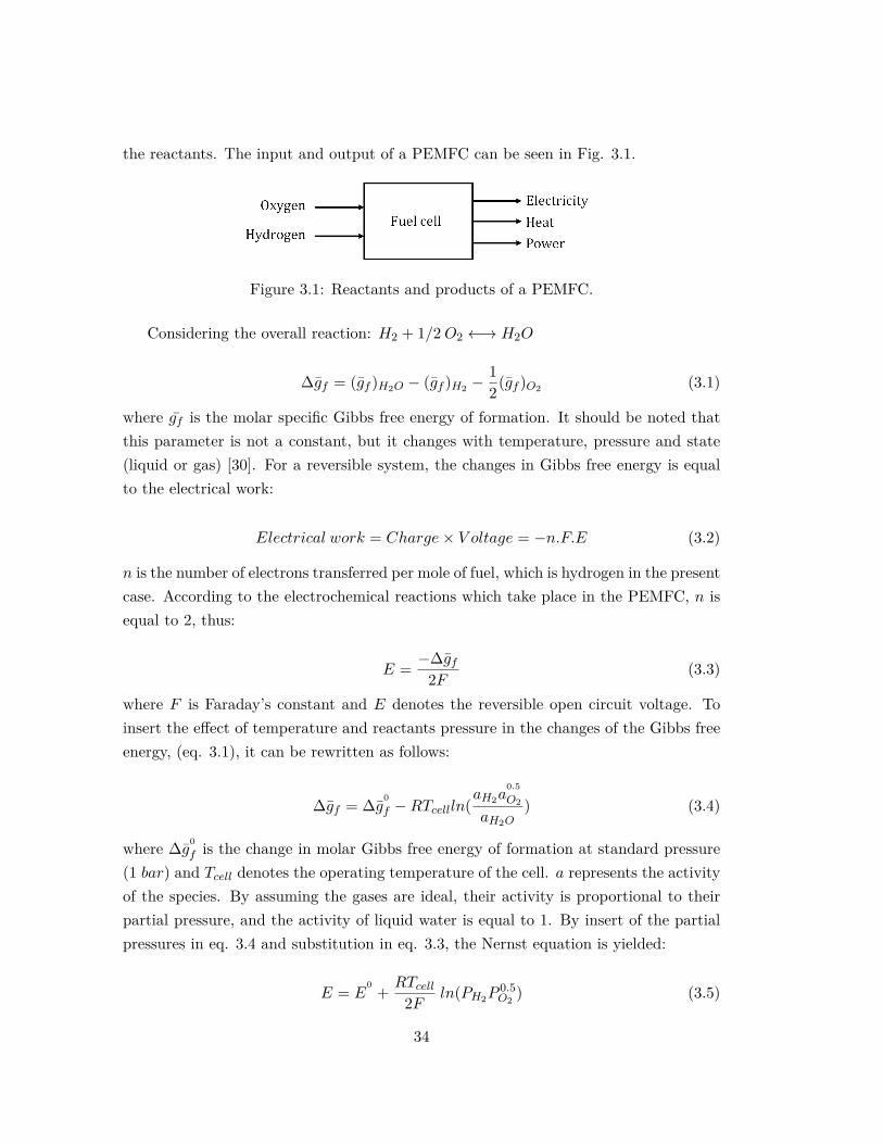
the reactants. The input and output of a PEMFC can be seen in Fig. 3.1.

Figure 3.1: Reactants and products of a PEMFC.

Considering the overall reaction: H2 + 1/2O2 ←→ H2O

∆gf = (gf )H2O − (gf )H2 −12(gf )O2 (3.1)

where gf is the molar specific Gibbs free energy of formation. It should be noted thatthis parameter is not a constant, but it changes with temperature, pressure and state(liquid or gas) [30]. For a reversible system, the changes in Gibbs free energy is equalto the electrical work:

Electrical work = Charge× V oltage = −n.F.E (3.2)

n is the number of electrons transferred per mole of fuel, which is hydrogen in the presentcase. According to the electrochemical reactions which take place in the PEMFC, n isequal to 2, thus:

E = −∆gf2F (3.3)

where F is Faraday’s constant and E denotes the reversible open circuit voltage. Toinsert the effect of temperature and reactants pressure in the changes of the Gibbs freeenergy, (eq. 3.1), it can be rewritten as follows:

∆gf = ∆g0f −RTcellln(

aH2a0.5O2

aH2O) (3.4)

where ∆g0f is the change in molar Gibbs free energy of formation at standard pressure

(1 bar) and Tcell denotes the operating temperature of the cell. a represents the activityof the species. By assuming the gases are ideal, their activity is proportional to theirpartial pressure, and the activity of liquid water is equal to 1. By insert of the partialpressures in eq. 3.4 and substitution in eq. 3.3, the Nernst equation is yielded:

E = E0 + RTcell

2F ln(PH2P0.5O2 ) (3.5)

34

where E0 = −∆gf

2F and represents the open circuit voltage at standard pressure. Dueto the low temperature gradient (less than 10C between the inlet reactants and outletproducts of the stack), the outlet temperature is applied to evaluate this parameter.PH2 and PO2 are assumed as average partial pressure of the hydrogen and the oxygenat the anode and the cathode compartment, respectively, and can be defined as:

PH2 =(yH2,out + yH2,in

2

)Pa (3.6)

PO2 =(yO2,out + yO2,in

2

)Pc (3.7)

where y is the molar fraction of the species. It should be noted that the pressure of theanode and the cathode compartment is the average pressure of the inlet reactants andthe product gases. The maximum efficiency of a fuel cell can be evaluated as:

ηmax = ∆gf∆hf

× 100% (3.8)

where ∆hf is the change in enthalpy of formation, which can be stated based on thehigher heating value (HHV) or the lower heating value (LHV). HHV and LHV refer tothe liquid product water or water vapor, respectively. The cell efficiency is given by:

ηcell = Vcell1.48 × 100%, refering to HHV,

ηcell = Vcell1.25 × 100%, refering to LHV

(3.9)

where Vcell is the cell voltage. 1.25 and 1.48 are the voltages which would be obtainedfrom a system with 100% efficiency. The fuel cell efficiency is given by:

ηstack = Uf .ηcell × 100% (3.10)

Uf is the utilization factor which is the mass flow of the reacted fuel in a cell proportionalto the input mass flow of the cell.

3.3 Electrochemical model of the PEM fuel cell

To investigate the behavior of the stack, we study the electrochemical process on a singlecell. The behavior of a single cell of the stack can be presented by the polarization curvein which the voltage of a single cell is given versus the current or current density of thecell. Basically the voltage over-potential includes three types of losses: the activation

35

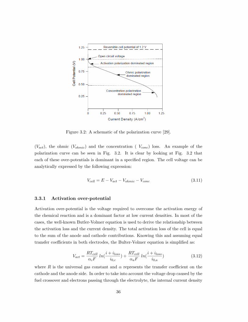
Figure 3.2: A schematic of the polarization curve [29].

(Vact), the ohmic (Vohmic) and the concentration ( Vconc) loss. An example of thepolarization curve can be seen in Fig. 3.2. It is clear by looking at Fig. 3.2 thateach of these over-potentials is dominant in a specified region. The cell voltage can beanalytically expressed by the following expression:

Vcell = E − Vact − Vohmic − Vconc (3.11)

3.3.1 Activation over-potential

Activation over-potential is the voltage required to overcome the activation energy ofthe chemical reaction and is a dominant factor at low current densities. In most of thecases, the well-known Butler-Volmer equation is used to derive the relationship betweenthe activation loss and the current density. The total activation loss of the cell is equalto the sum of the anode and cathode contributions. Knowing this and assuming equaltransfer coefficients in both electrodes, the Bulter-Volmer equation is simplified as:

Vact = RTcellαcF

ln( i+ ilossi0,c

) + RTcellαaF

ln( i+ ilossi0,a

) (3.12)

where R is the universal gas constant and α represents the transfer coefficient on thecathode and the anode side. In order to take into account the voltage drop caused by thefuel crossover and electrons passing through the electrolyte, the internal current density

36

(iloss) is added to the actual current density (i). For an effective performance of thecell, this parameter has to be reduced to the minimum. According to the literature, theinternal current density is usually neglected or is defined as a fixed value in the PEMFC.According to the recommendation by [34], iloss = 0.002 A/cm2 has been assumed in thecurrent study. To evaluate the transfer coefficient on the anode and the cathode side,respectively, the following equations are valid [35]:

αa = β.nel (3.13)

αc = (1− β).nel (3.14)

β is the symmetry factor whose value is very close to 0.5 [34]. nel indicates the numberof electrons in the rate step determining of the reaction whose value is 4 for the anodeand 1 for the cathode [34]. Another important issue for estimating the activation lossis the exchange current density, (i0), which is the rate constant for electrochemicalreactions and is a function of the temperature, the catalyst loading and the catalystspecific surface area [29]. Both analytical and experimental methods for evaluatingthis parameter can be found in the literature. However, this study uses an analyticalexpression that predicts the value of the exchange current density at the anode and thecathode separately [34].

i0,a = n.F.ka.exp

[(1− β).n.F.ER.Tcell

](3.15)

i0,c = n.F.kc.exp

[−β.n.F.ER.Tcell

](3.16)

where k is a function of the reaction speed which is initially unknown and can be foundafter calibration of the model. This will be elaborated later in this study. The amountof exchange current density on the anode is significantly higher than that on the cathodeside [36]. The typical ratio between the cathode and anode exchange current densitiesis stated as: i0,c/i0,a = 10−5, [30]. Therefore the contribution of the anode side to theactivation loss is often neglected. Only the activation over-potential on the cathode sideis taken into account when applying these set of equations.

Another method for calculating the activation loss is the one proposed by Berger [37]and widely used by other authors, [34, 38–41]. According to this method the conceptof the activation over-potential on the anode side can be expressed by the followingexpression:

37

Vact,a = −∆g

f

nF+ RTcell

nFln(4FAcellkac

?

H2)− RTcellnF

ln(i) (3.17)

where Acell is the cell active area, I is the current and c?H2denotes the concentration of

the liquid phase hydrogen on the anode side. Equation 5.11 can be simplified as followsafter insertation of the known parameters.

Vact,a = −(5.18× 10−6)∆gf + (4.309× 10−5)

×Tcell

[12.863 + ln

(Acellc

?

H2ka

i

)](3.18)

Likewise the activation over-potential on the cathode side can be expressed by:

Vact,c = RTcellαcnF

× ln [nFAcellkcexp(−

∆gf

RT

)×(

c?

O2

)1−αc (c?

H+

)1−αc (c?

H2O

)αc ]− ln(i) (3.19)

The proton concentration (c?H+) and water concentration (c?H2O) at the cathode

membrane/gas interface are relatively constant [42]. By incorporating these parametersinto kc and inserting the known parameters into the equation, it can be simplified as:

Vact,c = 1αc

[−(10.36× 10−6)∆gf + (8.62× 10−5)

×T(12.863 + ln(Acell) + ln(k′c) + (1− αc)ln(c?O2)− ln(i)

)] (3.20)

where k′c = kcc?

H++c?

H2O. The oxygen concentration (c?O2

) is defined by Henry’s law[40, 41]:

c?

O2 = PO2

5.08× 106 × exp(−498/Tcell)(3.21)

where PO2denotes the partial pressure of the oxygen. The sum of equations (5.12) and(5.14) gives the single expression for the activation over-potential:

Vact = ξ1 + ξ2 + ξ3Tcell[ln(c?

O2

)]+ ξ4Tcell [ln (i)] (3.22)

38

where:

ξ1 =∆g

f

nF−

∆gf

αcnF(3.23)

ξ2 = R

αcnFln

[nFAcellkc

(c?

H+

)1−αc (c?

H2O

)αc]+ R

nFln[4FAcellkac

?

H2

](3.24)

ξ3 = R(1− αc)αcnF

(3.25)

ξ4 = −(R

nF+ R

αcnF

)(3.26)

Collecting the experimental data during the various polarization curve records andmaking substitutions in the equation 3.22 yields a set of equations. Solving this set ofequations ξ terms can be evaluated.

3.3.2 Ohmic overpotential

Numerous equations for ohmic losses can be found in the literature; some of them arereviewed here, and those that are used in this study are mentioned at the end. Theohmic over-potential can be evaluated by:

Vohmic = (r.i) = (rion + rel).i (3.27)

in which rion is the ionic resistance of the membrane and rel represents the electronicresistance of the bipolar plates, cell interconnections and any other cell componentsthrough which electrons can flow. The contribution of the electronic resistance is verylow in comparison to the ionic resistance, and therefore it is usually neglected in thecalculations [43]. Amphlett et al. [38] proposed an analytic polynomial expression basedon collecting experimental data of a single cell with Nafion 117 as the membrane. Theequation is stated as:

Vohmic = (γ1 + γ2.Tcell + γ3.I).i (3.28)

where γ terms are constant and can be found using experimental data. According toempirical evaluation, γ2 and γ3 have to be negative and positive, respectively, so that

39

the ionic resistance decreases with the operating temperature and increases with thecurrent [34]. Another widely used equation for evaluating the ionic resistance is theone proposed by Mann et al. [39] and extensively used by other authors [34, 41]. Thiscorrelation has been yielded by analyzing literature data for different cells with Nafion117 included as the membrane.

rion =181.6.

[1 + 0.03.i+ 0.062

(Tcell303

)2.i2.5

].C1

(λmem − 0.634− 3.i) .exp [C2((Tcell − 303) /Tcell)].tm (3.29)

where λmem is the average water content of the membrane, which will be elaborated laterin this study. tm denotes the membrane thickness. 181.6/(λmem − 0.634) is the specificresistivity at zero current and 30C, and the other terms are the correction factors ifthe cell is not at 30C. The cell temperature (Tcell) is in kelvin in the aforementionedequation. Another alternative for evaluating the ionic resistance is stated as follows[29, 44]:

rion = tmσm

(3.30)

where σm is the membrane activity and can be correlated with the water content andtemperature using the following equation [29, 40, 41, 45].

σm = (0.005139λmem − 0.00326).exp(

1268( 1

303 −1

Tcell

))(3.31)

3.3.3 Concentration overpotential

The concentration over-potential arises from the concentration gradient of the reactantsand products between the flow channel and the catalyst reaction site. The reactionis faster at higher current density, and it increases the effect of concentration loss.At a limiting current where the transport of species is not fast enough to feed theelectrochemical reaction, the partial pressure of the reactants at the reaction site reacheszero and the voltage drastically drops. The limiting current density (il) is the maximumcurrent which can be drawn from the cell. The semi-empirical equation to calculate theconcentration loss is as follows [34, 46, 47]:

Vconc = RTcellnF

ln

(il

il − i

)(3.32)

il can be measured experimentally or calculated by theoretical equations [46]:

40

il = nF (qH2/O2) (3.33)

where q is the flux of hydrogen and oxygen gas corresponding to the limiting currentdensity of the anode and the cathode side, respectively. The empirical approach forevaluating the concentration loss can be expressed as follows [48]:

Vconc = m.exp(c.i) (3.34)

where m and c are empirical constants to be calculated by using the experimentaldata. In some other studies the following relation was referred to the concentrationover-potential [49]:

Vconc = R.Tcell4F ln

(yO4

yO3

)+ RTcell

2F ln(1− yW2

1− yW1) (3.35)

in which yO4 is the molar fraction of oxygen into the diffusion layer in the cathode flowchannel and yO3 is that out of the diffusion layer to the proton exchange membrane.yw1 is the molar fraction of water into the diffusion layer in the cathode flow channeland yw2 is that out of the diffusion layer to the proton exchange membrane. Since theconcentration loss is dominant at very high currents, which is not the case here, andsince steady-state behavior of the system is discussed in this study, this term does notplay a significant role and is neglected in the calculations.

3.3.4 Water management of the membrane

The water content in the polymer electrolyte plays a significant role in the PEMFCstack lifetime and the ionic resistance of the membrane. Low humidification in themembrane causes a rapid increase in the ionic resistance, and the high humidificationcauses too much liquid water to overflow into the reactant channels and fill the pores inthe electrodes. The water content profile through the membrane is unknown. Differentassumptions are made in the literature for determining water content across the mem-brane thickness. In this study a linear function is assumed, as proposed by [50, 51]. Byassuming a linear function for the water profile in the membrane, the mean value for themembrane water content is the average of the water content on the anode/membraneinterface (λa) and the cathode/membrane interface (λc):

λmem = (λa + λc2 ) (3.36)

41

The membrane water content at the electrodes/membrane interfaces can be definedthrough the following expression [45]:

λc&a = 0.043 + 17.18.aw − 39.85.a2w + 36.a3

w, 0 < aw < 1

λc&a = 14 + 1.4(aw − 1), 1 < aw≤3(3.37)

in which aw is water vapor activity and is defined by:

aw = PwPsat

(3.38)

λc&a is equal to 14 under ideal conditions, 100% relative humidity and can go as highas 22 under supersaturated conditions as reported by [45]. Replacing Pw with waterpartial pressure in the cathode or anode sides, aw in both electrodes can be calculated.Substituting aw with water vapor activity at the cathode or at the anode, λc and λa

can be evaluated, respectively. λmem may thus be calculated afterward. In order tohave high ionic conductivity in the membrane it should be fully hydrated. Hydrationcan be achieved by the humidification of the gases, or by designing the fuel cell to allowproduct water to hydrate the membrane [29]. We apply both methods in this study.Generally, the diffusion of water in the polymer electrolyte is expressed in two terms:one is the electro-osmotic drag phenomenon which is representative of the number ofwater molecules associated with protons (H+) while crossing through the membrane.But when the water is generated on the cathode side, this phenomenon occurs the otherway around. The water concentration gradient makes the water move from the cathodeto the anode side, which is called water back diffusion. The water molar flux due to theelectro-osmotic drag can be defined as:

JH2O,drag = 2ndragi

nF(3.39)

where:

ndrag = nsatdrag

λmem22 (3.40)

nsatdrag denotes saturated electro-osmotic drag and is experimentally evaluated between2.3 to 2.7 for the fully hydrated membrane in equilibrium with liquid water at 30-50[29], and this study assumes the amount to be 2.5 [45]. Back diffusion is also given bythe following equation:

JH2O,backdiffusion = ρdryMm

Dwdλmemdz

(3.41)

42

where ρdry is the dry density of Nafion, and Mm denotes the molecular weight of it. Dw

represents the water diffusivity, and z is the axis along the membrane thickness. Thenet water transport through the membrane is a combination of these two effects, theelectro-osmotic drag and back diffusion.

JH2O = JH2O,backdiffusion − JH2O,drag = ρdryMm

Dwdλmemdz

− 2ndragi

nF(3.42)

This is the net water which flows to the anode side and mixes with the fuel. The fuelis always saturated at the anode outlet. Liquid water is repulsed from the system via apurge valve, and the rest of the fuel is mixed with the inlet dry fuel, and the mixture isrecirculated back to the stack. Another parameter needed for calculating the net waterflux is the water diffusion which is a function of the membrane water content. There aremany attempts to define this parameter; the following literature [44, 45, 52, 53] suggeststhe following correlation:

Dw = Dλexp

(2416

( 1303 −

1Tcell + 273

))(3.43)

where Dw is the diffusion coefficient in the above equation. In this study the followingexpression for Dλ suggested by Springer et al. [45] is applied. This equation is onlyvalid for λmem > 4.

Dλ = 10−6(2.563− 0.33λmem + 0.0264λ2

mem − 0.000671λ3mem

)(3.44)

Murahashi et al. [52] suggests the equation as follows:

Dλ = 5.51× 10−7 × ndrag (3.45)

A further paper applies another expression for Dλ [44, 53] :

Dλ =

10−6, λmem < 2

10−6 (1 + 2 (λmem − 2)) , 2 ≤ λmem ≤ 3

10−6 (3− 1.67 (λmem − 3)) , 3 < λmem < 4.5

1.25× 10−6, λmem ≥ 4.5

(3.46)

43

3.4 Molar balance

Mass balance equations are applied separately for each composition in the reactants.We applied the following expression to find the molar flow rate of each species at theoutlet of the stack:

On the anode side:

nH2,out = nH2,in −((I + Iloss).Ncell

2.F

)(3.47)

nH2O,out,a = nH2O,in,a + (Jnet.Acell) (3.48)

On the cathode side:

nO2,out = nO2,in −12((I + Iloss).Ncell

2.F ) (3.49)

nH2O,out,c = nH2O,in,c + ((I + Iloss).Ncell

2.F )− (Jnet.Acell) (3.50)

nN2,in = nN2,out (3.51)

nCO2,in = nCO2,out (3.52)

nAr,in = nAr,out (3.53)

3.5 Other equations

In this process the power supplied by the system is known. Knowing the power andassuming that the cells are connected in series in the stack, one can evaluate the stackcurrent using the following equation:

Pstack = (Ncell.Vcell).I (3.54)

Faraday’s law is used to predict the mass flow rate of the reactants:

nH2 = I

n.F(3.55)

44

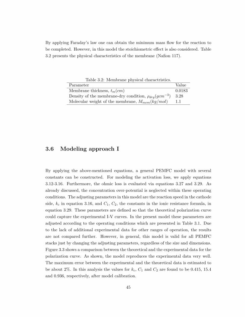
By applying Faraday’s law one can obtain the minimum mass flow for the reaction tobe completed. However, in this model the stoichiometric effect is also considered. Table3.2 presents the physical characteristics of the membrane (Nafion 117).

Table 3.2: Membrane physical charactristics.Parameter ValueMembrane thickness, tm(cm) 0.0183Density of the membrane-dry condition, ρdry(gcm−3) 3.28Molecular weight of the membrane, Mmem(kg/mol) 1.1

3.6 Modeling approach I

By applying the above-mentioned equations, a general PEMFC model with severalconstants can be constructed. For modeling the activation loss, we apply equations3.12-3.16. Furthermore, the ohmic loss is evaluated via equations 3.27 and 3.29. Asalready discussed, the concentration over-potential is neglected within these operatingconditions. The adjusting parameters in this model are the reaction speed in the cathodeside, kc in equation 3.16, and C1, C2, the constants in the ionic resistance formula, inequation 3.29. These parameters are defined so that the theoretical polarization curvecould capture the experimental I-V curves. In the present model these parameters areadjusted according to the operating conditions which are presented in Table 3.1. Dueto the lack of additional experimental data for other ranges of operation, the resultsare not compared further. However, in general, this model is valid for all PEMFCstacks just by changing the adjusting parameters, regardless of the size and dimensions.Figure 3.3 shows a comparison between the theoretical and the experimental data for thepolarization curve. As shown, the model reproduces the experimental data very well.The maximum error between the experimental and the theoretical data is estimated tobe about 2%. In this analysis the values for kc, C1 and C2 are found to be 0.415, 15.4and 0.936, respectively, after model calibration.

45

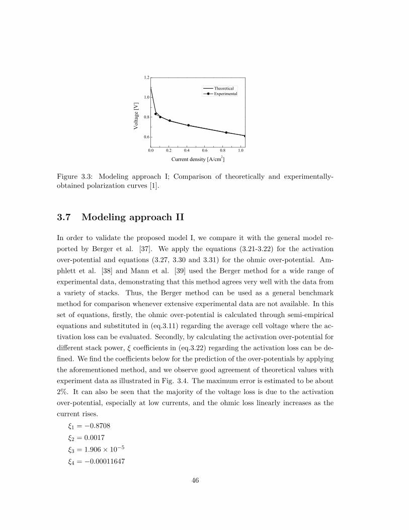
0.0 0.2 0.4 0.6 0.8 1.0

0.6

0.8

1.0

1.2

Vol

tage

[V]

Current density [A/cm2]

Theoretical Experimental

Figure 3.3: Modeling approach I; Comparison of theoretically and experimentally-obtained polarization curves [1].

3.7 Modeling approach II

In order to validate the proposed model I, we compare it with the general model re-ported by Berger et al. [37]. We apply the equations (3.21-3.22) for the activationover-potential and equations (3.27, 3.30 and 3.31) for the ohmic over-potential. Am-phlett et al. [38] and Mann et al. [39] used the Berger method for a wide range ofexperimental data, demonstrating that this method agrees very well with the data froma variety of stacks. Thus, the Berger method can be used as a general benchmarkmethod for comparison whenever extensive experimental data are not available. In thisset of equations, firstly, the ohmic over-potential is calculated through semi-empiricalequations and substituted in (eq.3.11) regarding the average cell voltage where the ac-tivation loss can be evaluated. Secondly, by calculating the activation over-potential fordifferent stack power, ξ coefficients in (eq.3.22) regarding the activation loss can be de-fined. We find the coefficients below for the prediction of the over-potentials by applyingthe aforementioned method, and we observe good agreement of theoretical values withexperiment data as illustrated in Fig. 3.4. The maximum error is estimated to be about2%. It can also be seen that the majority of the voltage loss is due to the activationover-potential, especially at low currents, and the ohmic loss linearly increases as thecurrent rises.

ξ1 = −0.8708ξ2 = 0.0017ξ3 = 1.906× 10−5

ξ4 = −0.00011647

46

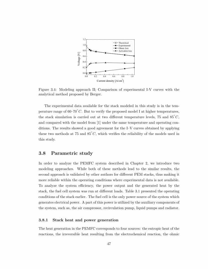
0.0 0.2 0.4 0.6 0.8 1.00.0

0.2

0.4

0.6

0.8

1.0

1.2

Vol

tage

[V]

Current density [A/cm2]

Theoretical Experimental Ohmic loss Activation loss

Figure 3.4: Modeling approach II; Comparison of experimental I-V curves with theanalytical method proposed by Berger.

The experimental data available for the stack modeled in this study is in the tem-perature range of 60–70

C. But to verify the proposed model I at higher temperatures,the stack simulation is carried out at two different temperature levels, 75 and 85

C,and compared with the model from [1] under the same temperature and operating con-ditions. The results showed a good agreement for the I–V curves obtained by applyingthese two methods at 75 and 85

C, which verifies the reliability of the models used inthis study.

3.8 Parametric study

In order to analyze the PEMFC system described in Chapter 2, we introduce twomodeling approaches. While both of these methods lead to the similar results, thesecond approach is validated by other authors for different PEM stacks, thus making itmore reliable within the operating conditions where experimental data is not available.To analyze the system efficiency, the power output and the generated heat by thestack, the fuel cell system was run at different loads. Table 3.1 presented the operatingconditions of the stack earlier. The fuel cell is the only power source of the system whichgenerates electrical power. A part of this power is utilized by the auxiliary components ofthe system, such as, the air compressor, recirculation pump, liquid pumps and radiator.

3.8.1 Stack heat and power generation

The heat generation in the PEMFC corresponds to four sources: the entropic heat of thereactions, the irreversible heat resulting from the electrochemical reaction, the ohmic

47

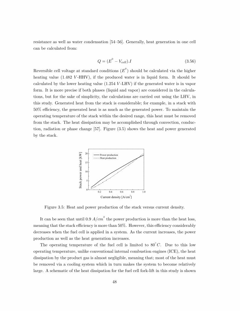
resistance as well as water condensation [54–56]. Generally, heat generation in one cellcan be calculated from:

Q = (E0 − Vcell).I (3.56)

Reversible cell voltage at standard conditions (E0) should be calculated via the higherheating value (1.482 V -HHV), if the produced water is in liquid form. It should becalculated by the lower heating value (1.254 V -LHV) if the generated water is in vaporform. It is more precise if both phases (liquid and vapor) are considered in the calcula-tions, but for the sake of simplicity, the calculations are carried out using the LHV, inthis study. Generated heat from the stack is considerable; for example, in a stack with50% efficiency, the generated heat is as much as the generated power. To maintain theoperating temperature of the stack within the desired range, this heat must be removedfrom the stack. The heat dissipation may be accomplished through convection, conduc-tion, radiation or phase change [57]. Figure (3.5) shows the heat and power generatedby the stack.

0.2 0.4 0.6 0.8 1.00

5

10

15

20

Stac

k po

wer

and

hea

t [kW

]

Current density [A/cm2]

Power production Heat production

Figure 3.5: Heat and power production of the stack versus current density.

It can be seen that until 0.9 A/cm2 the power production is more than the heat loss,meaning that the stack efficiency is more than 50%. However, this efficiency considerablydecreases when the fuel cell is applied in a system. As the current increases, the powerproduction as well as the heat generation increases.

The operating temperature of the fuel cell is limited to 80C. Due to this low

operating temperature, unlike conventional internal combustion engines (ICE), the heatdissipation by the product gas is almost negligible, meaning that; most of the heat mustbe removed via a cooling system which in turn makes the system to become relativelylarge. A schematic of the heat dissipation for the fuel cell fork-lift in this study is shown

48

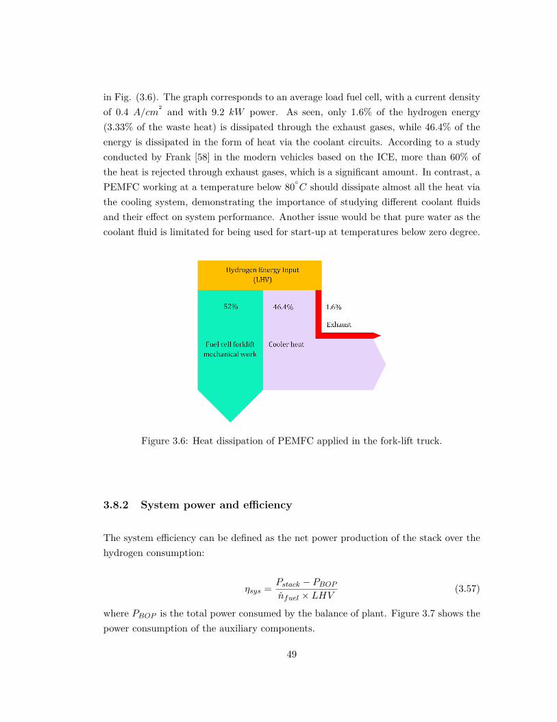
in Fig. (3.6). The graph corresponds to an average load fuel cell, with a current densityof 0.4 A/cm

2 and with 9.2 kW power. As seen, only 1.6% of the hydrogen energy(3.33% of the waste heat) is dissipated through the exhaust gases, while 46.4% of theenergy is dissipated in the form of heat via the coolant circuits. According to a studyconducted by Frank [58] in the modern vehicles based on the ICE, more than 60% ofthe heat is rejected through exhaust gases, which is a significant amount. In contrast, aPEMFC working at a temperature below 80

C should dissipate almost all the heat viathe cooling system, demonstrating the importance of studying different coolant fluidsand their effect on system performance. Another issue would be that pure water as thecoolant fluid is limitated for being used for start-up at temperatures below zero degree.

Figure 3.6: Heat dissipation of PEMFC applied in the fork-lift truck.

3.8.2 System power and efficiency

The system efficiency can be defined as the net power production of the stack over thehydrogen consumption:

ηsys = Pstack − PBOPnfuel × LHV

(3.57)

where PBOP is the total power consumed by the balance of plant. Figure 3.7 shows thepower consumption of the auxiliary components.

49

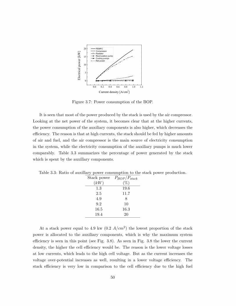
0.0 0.2 0.4 0.6 0.8 1.0 1.2

0

5

10

15

20

Elec

trica

l pow

er [k

W]

Current density [A/cm2]

PEMFC Compressor Radiator Recirculation pump Cooling pumps Net power

Figure 3.7: Power consumption of the BOP.

It is seen that most of the power produced by the stack is used by the air compressor.Looking at the net power of the system, it becomes clear that at the higher currents,the power consumption of the auxiliary components is also higher, which decreases theefficiency. The reason is that at high currents, the stack should be fed by higher amountsof air and fuel, and the air compressor is the main source of electricity consumptionin the system, while the electricity consumption of the auxiliary pumps is much lowercomparably. Table 3.3 summarizes the percentage of power generated by the stackwhich is spent by the auxillary components.

Table 3.3: Ratio of auxillary power consumption to the stack power production.Stack power PBOP /Pstack

(kW ) (%)1.3 19.62.5 11.74.9 89.2 1016.5 16.319.4 20

At a stack power equal to 4.9 kw (0.2 A/cm2) the lowest proportion of the stackpower is allocated to the auxiliary components, which is why the maximum systemefficiency is seen in this point (see Fig. 3.8). As seen in Fig. 3.8 the lower the currentdensity, the higher the cell efficiency would be. The reason is the lower voltage lossesat low currents, which leads to the high cell voltage. But as the current increases thevoltage over-potential increases as well, resulting in a lower voltage efficiency. Thestack efficiency is very low in comparison to the cell efficiency due to the high fuel

50

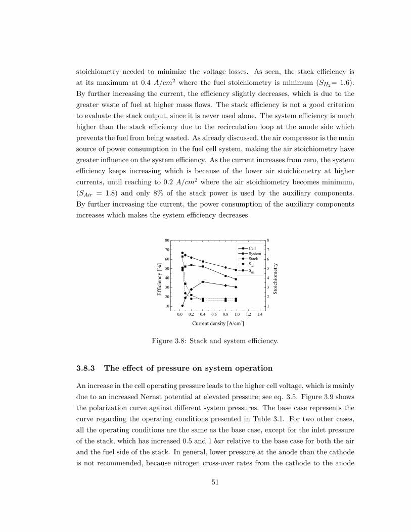
stoichiometry needed to minimize the voltage losses. As seen, the stack efficiency isat its maximum at 0.4 A/cm2 where the fuel stoichiometry is minimum (SH2= 1.6).By further increasing the current, the efficiency slightly decreases, which is due to thegreater waste of fuel at higher mass flows. The stack efficiency is not a good criterionto evaluate the stack output, since it is never used alone. The system efficiency is muchhigher than the stack efficiency due to the recirculation loop at the anode side whichprevents the fuel from being wasted. As already discussed, the air compressor is the mainsource of power consumption in the fuel cell system, making the air stoichiometry havegreater influence on the system efficiency. As the current increases from zero, the systemefficiency keeps increasing which is because of the lower air stoichiometry at highercurrents, until reaching to 0.2 A/cm2 where the air stoichiometry becomes minimum,(SAir = 1.8) and only 8% of the stack power is used by the auxiliary components.By further increasing the current, the power consumption of the auxiliary componentsincreases which makes the system efficiency decreases.

0.0 0.2 0.4 0.6 0.8 1.0 1.2 1.4

10

20

30

40

50

60

70

80

Cell System Stack SAir

SH2

Current density [A/cm2]

Effic

ienc

y [%

]

1

2

3

4

5

6

7

8

Sto

ichi

omet

ry

Figure 3.8: Stack and system efficiency.

3.8.3 The effect of pressure on system operation

An increase in the cell operating pressure leads to the higher cell voltage, which is mainlydue to an increased Nernst potential at elevated pressure; see eq. 3.5. Figure 3.9 showsthe polarization curve against different system pressures. The base case represents thecurve regarding the operating conditions presented in Table 3.1. For two other cases,all the operating conditions are the same as the base case, except for the inlet pressureof the stack, which has increased 0.5 and 1 bar relative to the base case for both the airand the fuel side of the stack. In general, lower pressure at the anode than the cathodeis not recommended, because nitrogen cross-over rates from the cathode to the anode

51

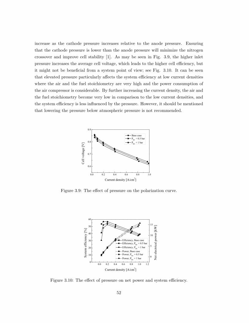
increase as the cathode pressure increases relative to the anode pressure. Ensuringthat the cathode pressure is lower than the anode pressure will minimize the nitrogencrossover and improve cell stability [1]. As may be seen in Fig. 3.9, the higher inletpressure increases the average cell voltage, which leads to the higher cell efficiency, butit might not be beneficial from a system point of view; see Fig. 3.10. It can be seenthat elevated pressure particularly affects the system efficiency at low current densitieswhere the air and the fuel stoichiometry are very high and the power consumption ofthe air compressor is considerable. By further increasing the current density, the air andthe fuel stoichiometry become very low in comparison to the low current densities, andthe system efficiency is less influenced by the pressure. However, it should be mentionedthat lowering the pressure below atmospheric pressure is not recommended.

0.0 0.2 0.4 0.6 0.8 1.0

0.6

0.7

0.8

0.9

Cel

l vol

tage

[V]

Current density [A/cm2]

Base case PBC + 0.5 bar PBC + 1 bar

Figure 3.9: The effect of pressure on the polarization curve.

0.0 0.2 0.4 0.6 0.8 1.0 1.20

10

20

30

40

50

60

Efficiency, Base case Efficiency, PBC + 0.5 bar Efficiency, PBC + 1 bar Power, Base case Power, PBC + 0.5 bar Power, PBC + 1 bar

Current density [A/cm2]

Syst

em e

ffic

ienc

y [%

]

0

5

10

15

Net

ele

ctric

al p

ower

[kW

]

Figure 3.10: The effect of pressure on net power and system efficiency.

52

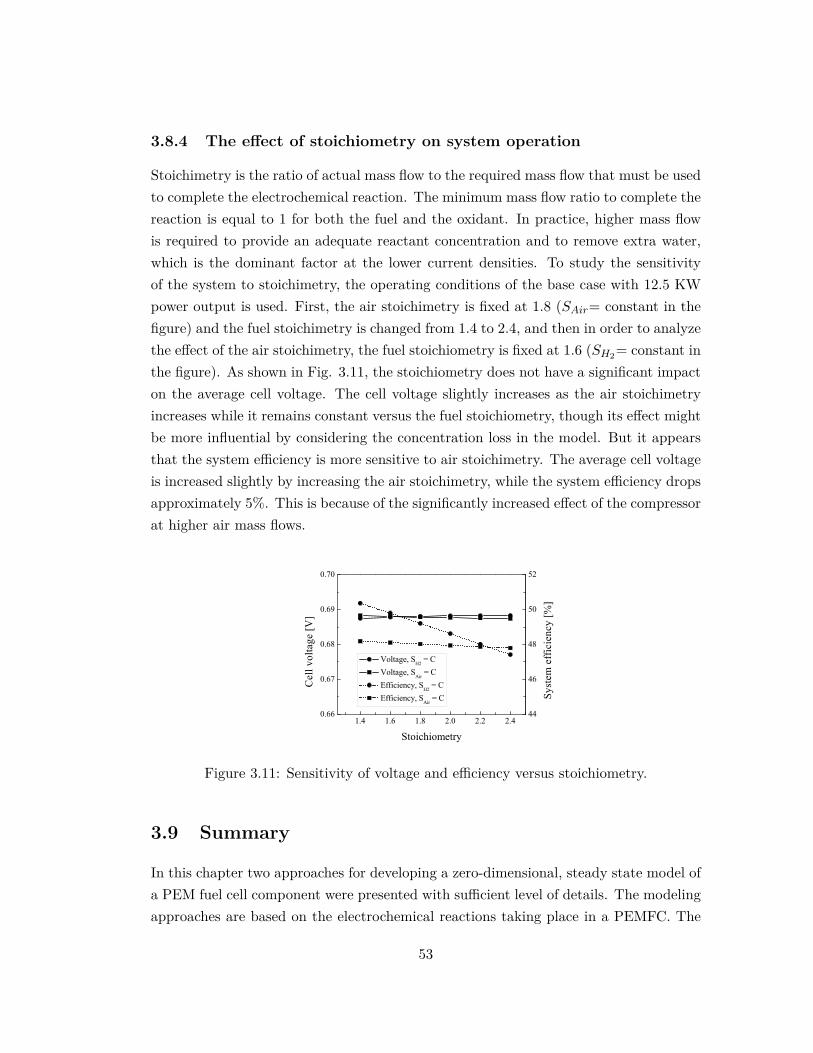
3.8.4 The effect of stoichiometry on system operation

Stoichimetry is the ratio of actual mass flow to the required mass flow that must be usedto complete the electrochemical reaction. The minimum mass flow ratio to complete thereaction is equal to 1 for both the fuel and the oxidant. In practice, higher mass flowis required to provide an adequate reactant concentration and to remove extra water,which is the dominant factor at the lower current densities. To study the sensitivityof the system to stoichimetry, the operating conditions of the base case with 12.5 KWpower output is used. First, the air stoichimetry is fixed at 1.8 (SAir= constant in thefigure) and the fuel stoichimetry is changed from 1.4 to 2.4, and then in order to analyzethe effect of the air stoichimetry, the fuel stoichiometry is fixed at 1.6 (SH2= constant inthe figure). As shown in Fig. 3.11, the stoichiometry does not have a significant impacton the average cell voltage. The cell voltage slightly increases as the air stoichimetryincreases while it remains constant versus the fuel stoichiometry, though its effect mightbe more influential by considering the concentration loss in the model. But it appearsthat the system efficiency is more sensitive to air stoichimetry. The average cell voltageis increased slightly by increasing the air stoichimetry, while the system efficiency dropsapproximately 5%. This is because of the significantly increased effect of the compressorat higher air mass flows.

1.4 1.6 1.8 2.0 2.2 2.40.66

0.67

0.68

0.69

0.70

Voltage, SH2 = C Voltage, SAir = C Efficiency, SH2 = C Efficiency, SAir = C

Stoichiometry

Cel

l vol

tage

[V]

44

46

48

50

52

Sys

tem

eff

icie

ncy

[%]

Figure 3.11: Sensitivity of voltage and efficiency versus stoichiometry.

3.9 Summary

In this chapter two approaches for developing a zero-dimensional, steady state model ofa PEM fuel cell component were presented with sufficient level of details. The modelingapproaches are based on the electrochemical reactions taking place in a PEMFC. The

53

models were validated against the experimental data from the stack manual, providedby the stack manufacturer (Ballard company). The polarization curve shows a verygood agreement with the experimental data. Afterwards, the behavior of the PEMFCin cooperation with the BOP in a system was presented in terms of power productionas well as efficiency. The next chapter presents system sensitivity to the operatingconditions as well as water and thermal management.

54

Chapter 4

Water and thermal management

4.1 Overview

The operating temperature of the fuel cell is usually in the range of 60-80C. The highertemperature of the stack can cause degradation in the membrane or catalyst while alower temperature of the stack is not favorable from kinetics point of view, it might alsocause flooding due to lower water saturation pressure at lower temperature, which is amajor concern in water management [54, 59, 60].

Two factors are critical in designing a cooling system for PEM fuel cells: firstly theoperating temperature of the stack is limited to 80

C which means that the temperaturedifference between the ambient air and exhaust gases is too low in compare to theconventional internal combustion engine’s cooling system. Secondly, the heat removalby the reactants and products is almost negligible and the entire waste heat mustbe removed by a cooling system. In order to ensure the stack operation within thedesired temperature range which is the main purpose of thermal management [55].These two factors cause a need for a relatively large radiator in automotive PEMFCsystems which is very challenging issue with the current technology. Rising the operatingtemperature of the fuel cell could be one way to improve the effectiveness of the currentcooling technologies. Besides, the high temperature fuel cell is more tolerant againstCO contaminations [59, 61, 62] and it gives the possibility of using other fuels besidepure hydrogen, though discussion on high temperature PEMFC is out of scope of thisresearch. Heat generated in the stack may be dissipated by conduction, convection,radiation or phase change [54, 57]. If the heat is not properly dissipated by the cooling

55

system, the stack temperature eventually increases and this will lead to a low relativehumidity of the membrane, which decrease the ionic conductivity of the membrane.Therefore water management should also be considered beside the thermal managementof the stack. Cooling methods are determined greatly by the size of the fuel cell [57].The typical methods for heat management of the stack are listed as below [54, 57].

• Cooling with heat spreaders

• Cooling with cathode air flow

• Cooling with separate air flow

• Liquid cooling

• Phase change cooling

Liquid coolants have much higher heat capacity than gas coolants, which makes themmore efficient for cooling application especially in PEMFC larger than 5 kW. The mosttypical liquid coolants are deionized water, water- ethylene glycol mixture. Due to wideapplication of liquid coolants in automotive industry, numerous effort has been made foroptimization of the cooling system either for finding alternative coolants or optimizingcooling channel design and geometry.

4.2 Voltage sensitivity versus relative humidity

In order to avoid high ionic resistance it is very important to keep the membrane hu-midity as high as possible during the stack operation. Since oxygen is taken directlyfrom the ambient air, it has low relative humidity at the cathode inlet with the tem-perature around 60

C. This is the reason to use an air humidifier in the system beforethe stack to increase the relative humidity of the incoming air to the desired values.The operating temperature of the fuel cell is around 62-70

C and as the temperatureincreases; higher amount of vapor is needed to keep the humidity at the same level.Since water is one of the byproducts of the chemical reaction in the stack, it is of greatimportance to keep the membrane humidity within the desired level. Humidity controlis a challenging issue and it can cause 20-40% voltage drop if the humidification is notcontrolled properly [17, 44, 63, 64]. Figure 4.1 shows the effect of relative humidity ofthe inlet air on the cell voltage.

56

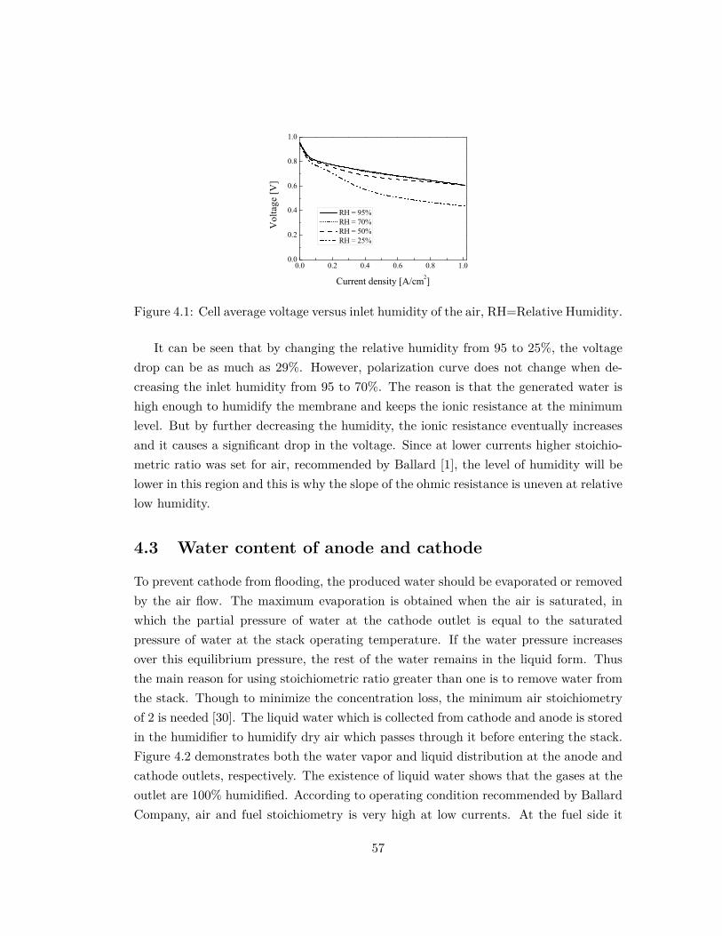
0.0 0.2 0.4 0.6 0.8 1.00.0

0.2

0.4

0.6

0.8

1.0

Vol

tage

[V]

Current density [A/cm2]

RH = 95% RH = 70% RH = 50% RH = 25%

Figure 4.1: Cell average voltage versus inlet humidity of the air, RH=Relative Humidity.

It can be seen that by changing the relative humidity from 95 to 25%, the voltagedrop can be as much as 29%. However, polarization curve does not change when de-creasing the inlet humidity from 95 to 70%. The reason is that the generated water ishigh enough to humidify the membrane and keeps the ionic resistance at the minimumlevel. But by further decreasing the humidity, the ionic resistance eventually increasesand it causes a significant drop in the voltage. Since at lower currents higher stoichio-metric ratio was set for air, recommended by Ballard [1], the level of humidity will belower in this region and this is why the slope of the ohmic resistance is uneven at relativelow humidity.

4.3 Water content of anode and cathode

To prevent cathode from flooding, the produced water should be evaporated or removedby the air flow. The maximum evaporation is obtained when the air is saturated, inwhich the partial pressure of water at the cathode outlet is equal to the saturatedpressure of water at the stack operating temperature. If the water pressure increasesover this equilibrium pressure, the rest of the water remains in the liquid form. Thusthe main reason for using stoichiometric ratio greater than one is to remove water fromthe stack. Though to minimize the concentration loss, the minimum air stoichiometryof 2 is needed [30]. The liquid water which is collected from cathode and anode is storedin the humidifier to humidify dry air which passes through it before entering the stack.Figure 4.2 demonstrates both the water vapor and liquid distribution at the anode andcathode outlets, respectively. The existence of liquid water shows that the gases at theoutlet are 100% humidified. According to operating condition recommended by BallardCompany, air and fuel stoichiometry is very high at low currents. At the fuel side it

57

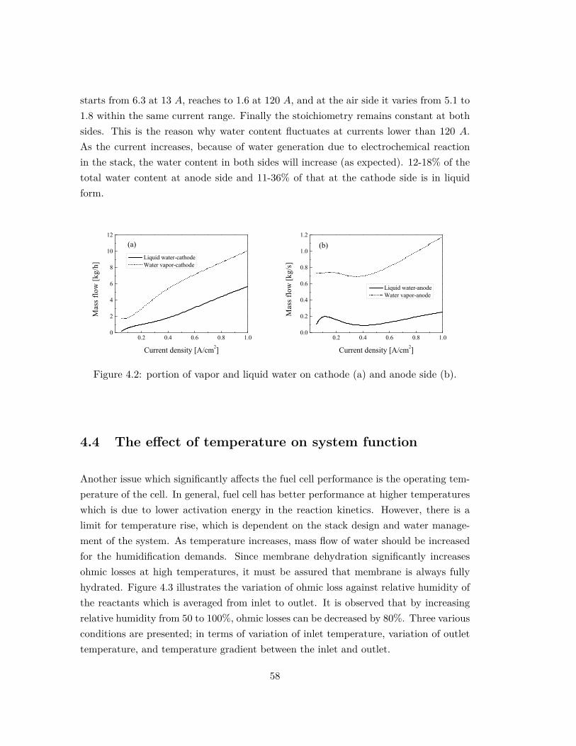
starts from 6.3 at 13 A, reaches to 1.6 at 120 A, and at the air side it varies from 5.1 to1.8 within the same current range. Finally the stoichiometry remains constant at bothsides. This is the reason why water content fluctuates at currents lower than 120 A.As the current increases, because of water generation due to electrochemical reactionin the stack, the water content in both sides will increase (as expected). 12-18% of thetotal water content at anode side and 11-36% of that at the cathode side is in liquidform.

0.2 0.4 0.6 0.8 1.00

2

4

6

8

10

12(a)

Mas

s flo

w [k

g/h]

Current density [A/cm2]

Liquid water-cathode Water vapor-cathode

0.2 0.4 0.6 0.8 1.00.0

0.2

0.4

0.6

0.8

1.0

1.2

(b)

Mas

s flo

w [k

g/s]

Current density [A/cm2]

Liquid water-anode Water vapor-anode

Figure 4.2: portion of vapor and liquid water on cathode (a) and anode side (b).

4.4 The effect of temperature on system function

Another issue which significantly affects the fuel cell performance is the operating tem-perature of the cell. In general, fuel cell has better performance at higher temperatureswhich is due to lower activation energy in the reaction kinetics. However, there is alimit for temperature rise, which is dependent on the stack design and water manage-ment of the system. As temperature increases, mass flow of water should be increasedfor the humidification demands. Since membrane dehydration significantly increasesohmic losses at high temperatures, it must be assured that membrane is always fullyhydrated. Figure 4.3 illustrates the variation of ohmic loss against relative humidity ofthe reactants which is averaged from inlet to outlet. It is observed that by increasingrelative humidity from 50 to 100%, ohmic losses can be decreased by 80%. Three variousconditions are presented; in terms of variation of inlet temperature, variation of outlettemperature, and temperature gradient between the inlet and outlet.

58

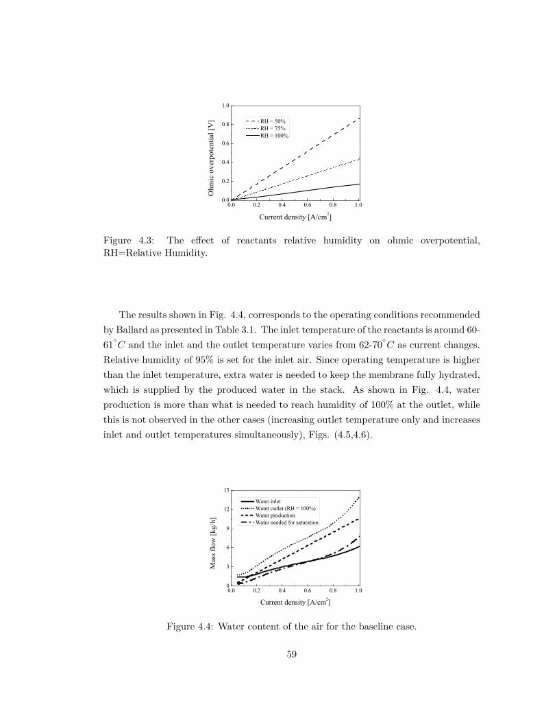
0.0 0.2 0.4 0.6 0.8 1.00.0

0.2

0.4

0.6

0.8

1.0

Ohm

ic o

verp

oten

tial [

V]

Current density [A/cm2]

RH = 50% RH = 75% RH = 100%

Figure 4.3: The effect of reactants relative humidity on ohmic overpotential,RH=Relative Humidity.

The results shown in Fig. 4.4, corresponds to the operating conditions recommendedby Ballard as presented in Table 3.1. The inlet temperature of the reactants is around 60-61

C and the inlet and the outlet temperature varies from 62-70C as current changes.

Relative humidity of 95% is set for the inlet air. Since operating temperature is higherthan the inlet temperature, extra water is needed to keep the membrane fully hydrated,which is supplied by the produced water in the stack. As shown in Fig. 4.4, waterproduction is more than what is needed to reach humidity of 100% at the outlet, whilethis is not observed in the other cases (increasing outlet temperature only and increasesinlet and outlet temperatures simultaneously), Figs. (4.5,4.6).

0.0 0.2 0.4 0.6 0.8 1.00

3

6

9

12

15

Mas

s flo

w [k

g/h]

Current density [A/cm2]

Water inlet Water outlet (RH = 100%) Water production Water needed for saturation

Figure 4.4: Water content of the air for the baseline case.

59

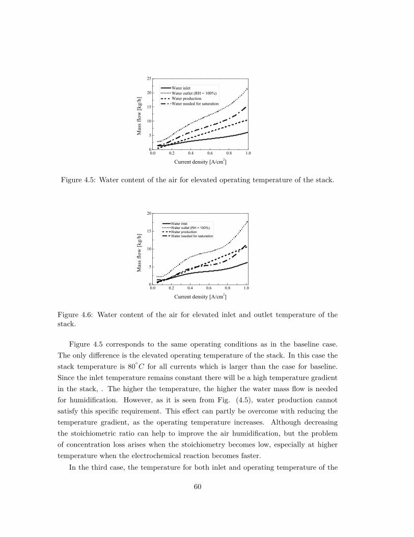
0.0 0.2 0.4 0.6 0.8 1.00

5

10

15

20

25

Mas

s flo

w [k

g/h]

Current density [A/cm2]

Water inlet Water outlet (RH = 100%) Water production Water needed for saturation

Figure 4.5: Water content of the air for elevated operating temperature of the stack.

0.0 0.2 0.4 0.6 0.8 1.00

5

10

15

20

Mas

s flo

w [k

g/h]

Current density [A/cm2]

Water inlet Water outlet (RH = 100%) Water production Water needed for saturation

Figure 4.6: Water content of the air for elevated inlet and outlet temperature of thestack.

Figure 4.5 corresponds to the same operating conditions as in the baseline case.The only difference is the elevated operating temperature of the stack. In this case thestack temperature is 80

C for all currents which is larger than the case for baseline.Since the inlet temperature remains constant there will be a high temperature gradientin the stack, . The higher the temperature, the higher the water mass flow is neededfor humidification. However, as it is seen from Fig. (4.5), water production cannotsatisfy this specific requirement. This effect can partly be overcome with reducing thetemperature gradient, as the operating temperature increases. Although decreasingthe stoichiometric ratio can help to improve the air humidification, but the problemof concentration loss arises when the stoichiometry becomes low, especially at highertemperature when the electrochemical reaction becomes faster.

In the third case, the temperature for both inlet and operating temperature of the

60

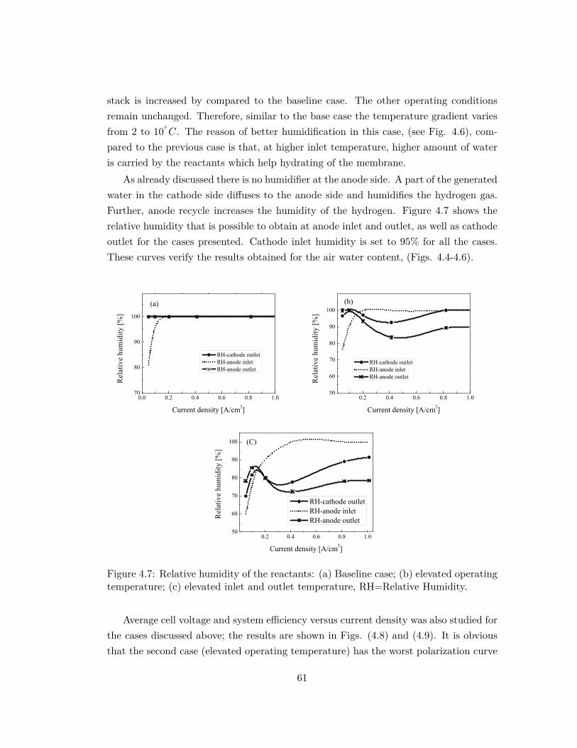
stack is increased by compared to the baseline case. The other operating conditionsremain unchanged. Therefore, similar to the base case the temperature gradient variesfrom 2 to 10

C. The reason of better humidification in this case, (see Fig. 4.6), com-pared to the previous case is that, at higher inlet temperature, higher amount of wateris carried by the reactants which help hydrating of the membrane.

As already discussed there is no humidifier at the anode side. A part of the generatedwater in the cathode side diffuses to the anode side and humidifies the hydrogen gas.Further, anode recycle increases the humidity of the hydrogen. Figure 4.7 shows therelative humidity that is possible to obtain at anode inlet and outlet, as well as cathodeoutlet for the cases presented. Cathode inlet humidity is set to 95% for all the cases.These curves verify the results obtained for the air water content, (Figs. 4.4-4.6).

0.0 0.2 0.4 0.6 0.8 1.070

80

90

100

(a)

Rel

ativ

e hu

mid

ity [%

]

Current density [A/cm2]

RH-cathode outlet RH-anode inlet RH-anode outlet

0.2 0.4 0.6 0.8 1.050

60

70

80

90

100(b)

Rel

ativ

e hu

mid

ity [%

]

Current density [A/cm2]

RH-cathode outlet RH-anode inlet RH-anode outlet

0.2 0.4 0.6 0.8 1.050

60

70

80

90

100 (C)

RH-cathode outlet RH-anode inlet RH-anode outlet

Rel

ativ

e hu

mid

ity [%

]

Current density [A/cm2]

RH-cathode outlet RH-anode inlet RH-anode outlet

Figure 4.7: Relative humidity of the reactants: (a) Baseline case; (b) elevated operatingtemperature; (c) elevated inlet and outlet temperature, RH=Relative Humidity.

Average cell voltage and system efficiency versus current density was also studied forthe cases discussed above; the results are shown in Figs. (4.8) and (4.9). It is obviousthat the second case (elevated operating temperature) has the worst polarization curve

61

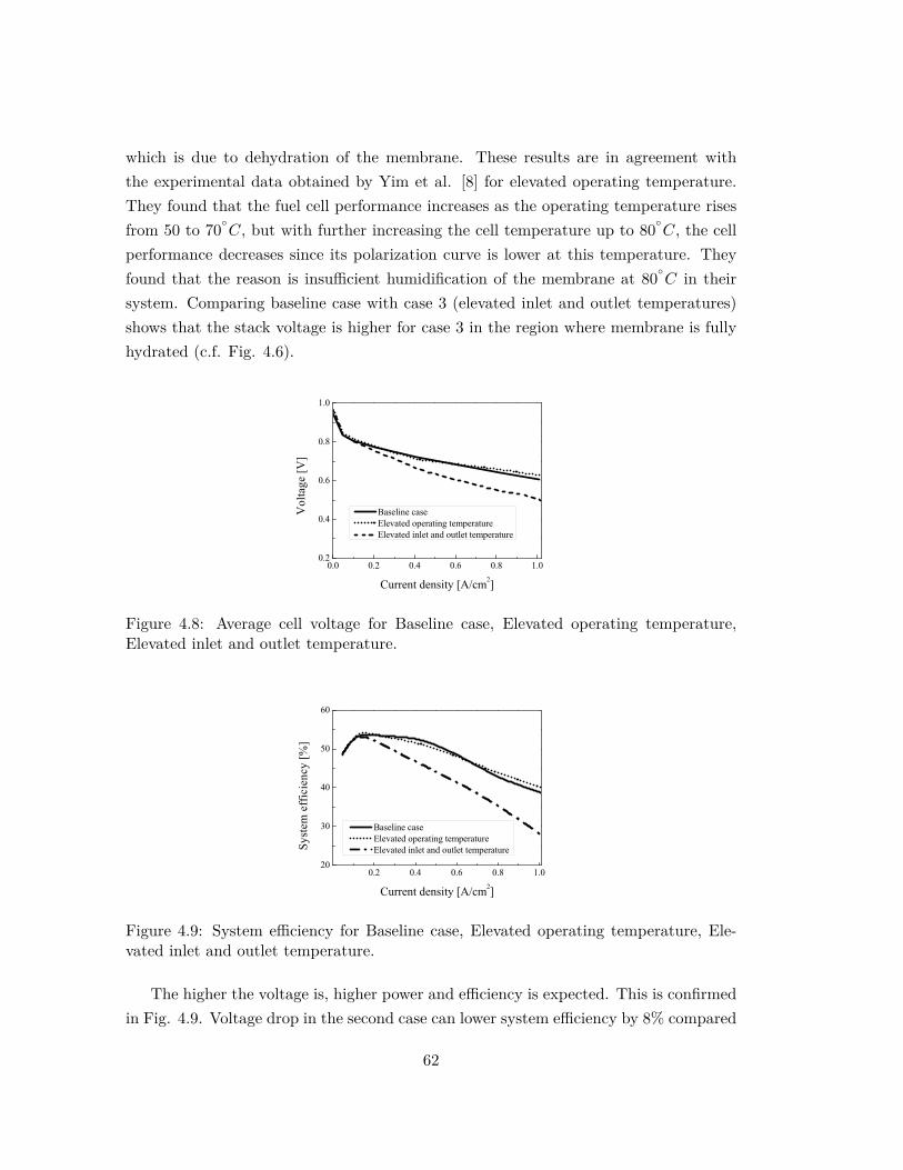
which is due to dehydration of the membrane. These results are in agreement withthe experimental data obtained by Yim et al. [8] for elevated operating temperature.They found that the fuel cell performance increases as the operating temperature risesfrom 50 to 70

C, but with further increasing the cell temperature up to 80C, the cell

performance decreases since its polarization curve is lower at this temperature. Theyfound that the reason is insufficient humidification of the membrane at 80

C in theirsystem. Comparing baseline case with case 3 (elevated inlet and outlet temperatures)shows that the stack voltage is higher for case 3 in the region where membrane is fullyhydrated (c.f. Fig. 4.6).

0.0 0.2 0.4 0.6 0.8 1.00.2

0.4

0.6

0.8

1.0

Vol

tage

[V]

Current density [A/cm2]

Baseline case Elevated operating temperature Elevated inlet and outlet temperature

Figure 4.8: Average cell voltage for Baseline case, Elevated operating temperature,Elevated inlet and outlet temperature.

0.2 0.4 0.6 0.8 1.020

30

40

50

60

Syst

em e

ffic

ienc

y [%

]

Current density [A/cm2]

Baseline case Elevated operating temperature Elevated inlet and outlet temperature

Figure 4.9: System efficiency for Baseline case, Elevated operating temperature, Ele-vated inlet and outlet temperature.

The higher the voltage is, higher power and efficiency is expected. This is confirmedin Fig. 4.9. Voltage drop in the second case can lower system efficiency by 8% compared

62

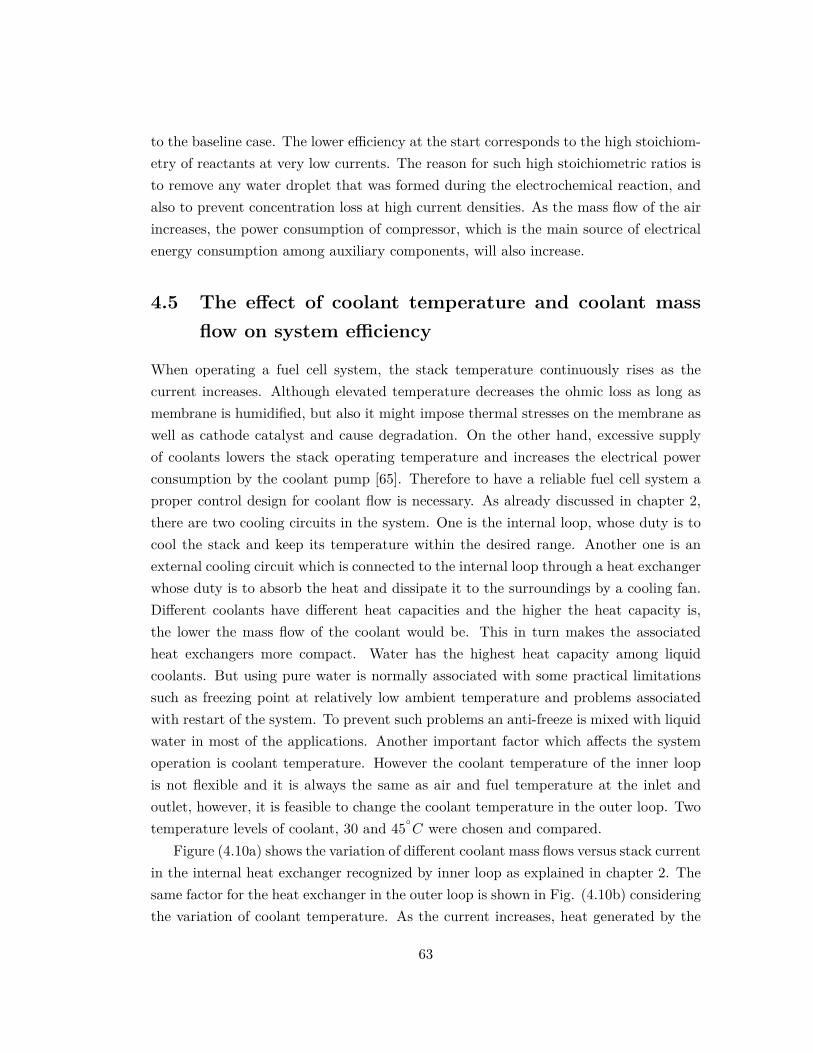
to the baseline case. The lower efficiency at the start corresponds to the high stoichiom-etry of reactants at very low currents. The reason for such high stoichiometric ratios isto remove any water droplet that was formed during the electrochemical reaction, andalso to prevent concentration loss at high current densities. As the mass flow of the airincreases, the power consumption of compressor, which is the main source of electricalenergy consumption among auxiliary components, will also increase.

4.5 The effect of coolant temperature and coolant massflow on system efficiency

When operating a fuel cell system, the stack temperature continuously rises as thecurrent increases. Although elevated temperature decreases the ohmic loss as long asmembrane is humidified, but also it might impose thermal stresses on the membrane aswell as cathode catalyst and cause degradation. On the other hand, excessive supplyof coolants lowers the stack operating temperature and increases the electrical powerconsumption by the coolant pump [65]. Therefore to have a reliable fuel cell system aproper control design for coolant flow is necessary. As already discussed in chapter 2,there are two cooling circuits in the system. One is the internal loop, whose duty is tocool the stack and keep its temperature within the desired range. Another one is anexternal cooling circuit which is connected to the internal loop through a heat exchangerwhose duty is to absorb the heat and dissipate it to the surroundings by a cooling fan.Different coolants have different heat capacities and the higher the heat capacity is,the lower the mass flow of the coolant would be. This in turn makes the associatedheat exchangers more compact. Water has the highest heat capacity among liquidcoolants. But using pure water is normally associated with some practical limitationssuch as freezing point at relatively low ambient temperature and problems associatedwith restart of the system. To prevent such problems an anti-freeze is mixed with liquidwater in most of the applications. Another important factor which affects the systemoperation is coolant temperature. However the coolant temperature of the inner loopis not flexible and it is always the same as air and fuel temperature at the inlet andoutlet, however, it is feasible to change the coolant temperature in the outer loop. Twotemperature levels of coolant, 30 and 45

C were chosen and compared.Figure (4.10a) shows the variation of different coolant mass flows versus stack current

in the internal heat exchanger recognized by inner loop as explained in chapter 2. Thesame factor for the heat exchanger in the outer loop is shown in Fig. (4.10b) consideringthe variation of coolant temperature. As the current increases, heat generated by the

63

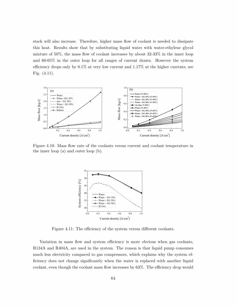
stack will also increase. Therefore, higher mass flow of coolant is needed to dissipatethis heat. Results show that by substituting liquid water with water-ethylene glycolmixture of 50%, the mass flow of coolant increases by about 32-33% in the inner loopand 60-65% in the outer loop for all ranges of current drawn. However the systemefficiency drops only by 0.1% at very low current and 1.17% at the higher currents, seeFig. (4.11).

0.2 0.4 0.6 0.8 1.00.0

0.5

1.0

1.5

2.0

2.5

3.0

Water Water +EG 10% ater + EG 30% Water + EG 50% R134A R404A

Mas

s flo

w [k

g/s]

Current density [A/cm2]

(a)

0.0 0.2 0.4 0.6 0.8 1.00.0

0.2

0.4

0.6

0.8

1.0 (b)

Mas

s flo

w [k

g/s]

Current density [A/cm2]

Water (T=30oC) Water + EG 10% (T=30oC) Water + EG 30% (T=30oC) Water + EG 50% (T=30oC) Air (fan, T=30oC) Water (T=45oC) Water + EG 10% (T=45oC) Water + EG 30% (T=45oC) Water + EG 50% (T=45oC)

Figure 4.10: Mass flow rate of the coolants versus current and coolant temperature inthe inner loop (a) and outer loop (b).

0.0 0.2 0.4 0.6 0.8 1.0

30

35

40

45

50

55

Syst

em e

ffic

ienc

y [%

]

Current density [A/cm2]

Water Water + EG 10% Water + EG 30% Water + EG 50% R134A

Figure 4.11: The efficiency of the system versus different coolants.

Variation in mass flow and system efficiency is more obvious when gas coolants,R134A and R404A, are used in the system. The reason is that liquid pump consumesmuch less electricity compared to gas compressors, which explains why the system ef-ficiency does not change significantly when the water is replaced with another liquidcoolant, even though the coolant mass flow increases by 63%. The efficiency drop would

64

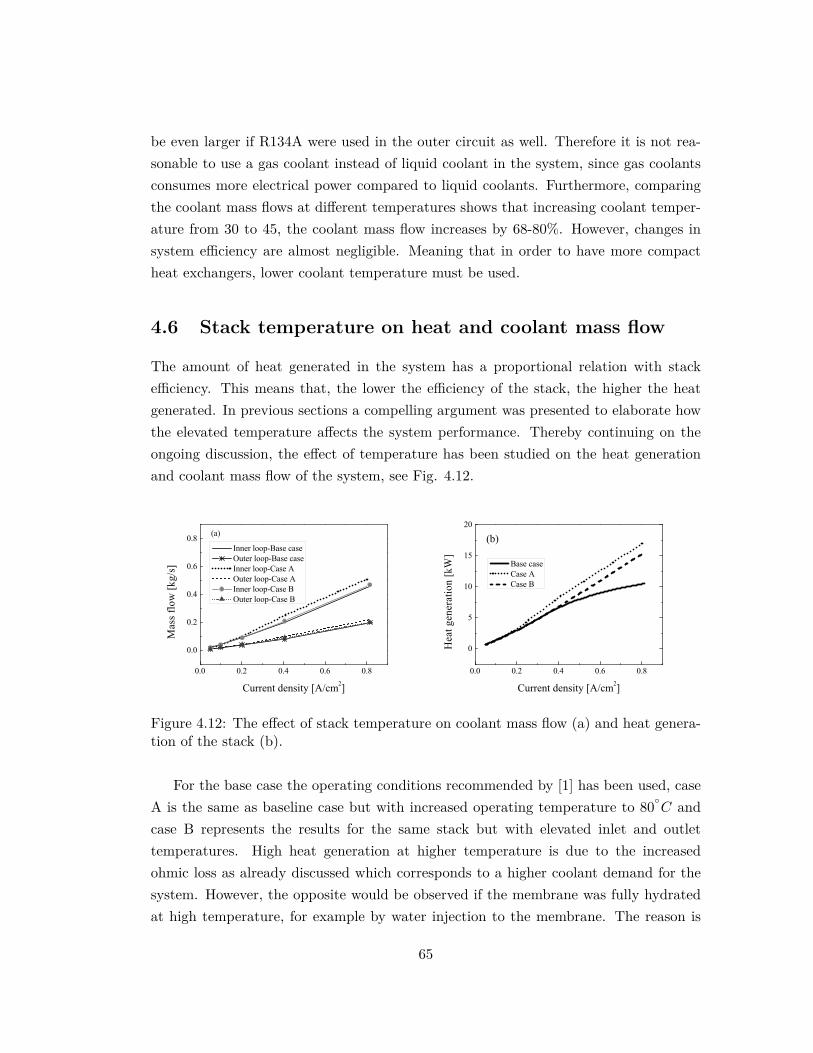
be even larger if R134A were used in the outer circuit as well. Therefore it is not rea-sonable to use a gas coolant instead of liquid coolant in the system, since gas coolantsconsumes more electrical power compared to liquid coolants. Furthermore, comparingthe coolant mass flows at different temperatures shows that increasing coolant temper-ature from 30 to 45, the coolant mass flow increases by 68-80%. However, changes insystem efficiency are almost negligible. Meaning that in order to have more compactheat exchangers, lower coolant temperature must be used.

4.6 Stack temperature on heat and coolant mass flow

The amount of heat generated in the system has a proportional relation with stackefficiency. This means that, the lower the efficiency of the stack, the higher the heatgenerated. In previous sections a compelling argument was presented to elaborate howthe elevated temperature affects the system performance. Thereby continuing on theongoing discussion, the effect of temperature has been studied on the heat generationand coolant mass flow of the system, see Fig. 4.12.

0.0 0.2 0.4 0.6 0.8

0.0

0.2

0.4

0.6

0.8 (a)

Mas

s flo

w [k

g/s]

Current density [A/cm2]

Inner loop-Base case Outer loop-Base case Inner loop-Case A Outer loop-Case A Inner loop-Case B Outer loop-Case B

0.0 0.2 0.4 0.6 0.8

0

5

10

15

20

(b)

Hea

t gen

erat

ion

[kW

]

Current density [A/cm2]

Base case Case A Case B

Figure 4.12: The effect of stack temperature on coolant mass flow (a) and heat genera-tion of the stack (b).

For the base case the operating conditions recommended by [1] has been used, caseA is the same as baseline case but with increased operating temperature to 80

C andcase B represents the results for the same stack but with elevated inlet and outlettemperatures. High heat generation at higher temperature is due to the increasedohmic loss as already discussed which corresponds to a higher coolant demand for thesystem. However, the opposite would be observed if the membrane was fully hydratedat high temperature, for example by water injection to the membrane. The reason is

65

that for constant amount of heat, larger temperature gradient of the coolant can leadto a more compact heat exchanger; though in that case the size of the radiator willincrease.

4.7 Summary

Water and thermal management of the stack as well as BOP were investigated in thischapter. The summary of the results are presented as follows:

For the baseline case 12-18% of the total water content at anode outlet and 11-36%of that at the cathode outlet is in liquid form which confirms the proper humidificationof the system. Variations in humidity level of inlet air from 25 to 95%, the voltage maydrop by 29%. However polarization curve does not change while decreasing the inlethumidity from 95 to 70%.

Another issue which significantly affects the fuel cell performance is the operatingtemperature of the cell. By increasing the stack temperature to 80

C for all the currentsdrawn and keeping the inlet temperatures unchanged, system efficiency decreases by 8%compared to the baseline case. The higher the temperature, the higher the mass flowis needed for humidification and water production cannot meet this requirement. Thiseffect can be partly improved by reducing the temperature gradient as the operatingtemperature increases.

By substituting liquid water with water-ethylene glycol mixture of 50%, the massflow of coolant increases with about 32-33% in the inner loop and 60-65% in the outerloop for all ranges of current. However, the system efficiency drops from 0.1 at verylow current to 1.17% at the highest current studied here (300A , 1A/cm2 ). Thevariation of mass flow and efficiency is more significant when the gas coolants, R134Aand R404A, are used in the system. Therefore, it is not reasonable to use gases coolantsin the system because they consume most of the electrical power and thereby systemefficiencies decreases considerably. Finally comparing the coolant mass flows at differenttemperatures show that by increasing coolant temperature from 30 to 45

C, mass flowincreases by 68-80%. Meaning that to have more compact heat exchangers, then lowertemperature for the coolant is advantageous. However, the efficiency differences will benegligible.

66

Chapter 5

Numerical Analysis of TransportPhenomena for Designing ofEjector in a PEM Forklift System

In the present study, Computational Fluid Dynamics (CFD) technique is used todesign an ejector for anode recirculation in an automotive PEMFC system. A CFDmodel is firstly established and tested against well-documented and relevant solutionsfrom the literature, and then used for different ejector geometries under different oper-ating conditions. Results showed that a single ejector with optimized geometry cannotcover the required recirculation in the entire range of the fuel cell current. Having twoejectors for different ranges of currents is thus proposed as an alternative solution inwhich the system can better take the advantage of ejectors for recirculation purpose. Inaddition, the operating mode of one variable nozzle ejector has been investigated andcompared with aforementioned cases.

5.1 Overview

PEMFC (Polymer Exchange Membrane Fuel Cell) is one alternative to replace theinternal combustion engines (ICE). There are many auxiliary components associatedwith fuel cell in the system which should regulate the operating conditions of the stackunder various load requests. The fuel delivery system is one of the subsystems whichsupplies hydrogen to the system from high pressure vessel. The extra hydrogen is alwayssupplied to the system for several reasons, mainly to prevent the hydrogen starvation of

67

the stack at the dynamic load request, further to remove any liquid water which mightbe condensed in the anode gas channels, and finally humidifying the fuel at the anodeside [66, 67].

In order to keep the system efficiency as high as possible the fuel recirculation is anecessity. In most of fuel cell systems a pump is used for recirculation of unconsumedhydrogen. Although the pump uses comparably significant amount of power in thesystem, this is not the main reason to replace the pump with an alternative solution. Inparticular electric pump cannot get accustomed with the liquid water which might existin the hydrogen due to condensation of the water vapor [68]. In more advanced solutions,the fuel cell delivery system comprises of an ejector and a pump, which work togetheror separately under different load requests [67]. Applying an ejector for recirculationin PEMFC automotive systems is very beneficial in terms of system efficiency, simplestructure, operation and maintenance (lack of moving parts).

The ejector in PEMFC systems needs significantly more optimized design in orderto operate properly within the practical operation mode. A small deviation from theoptimum geometry might drastically lower its operation, which is a major reason whycommercial ejectors cannot meet the requirements of a PEMFC system. This subjectbecomes even more important at the secondary flow (anode exhaust) which containshumidified hydrogen with higher molecular weight compared to the dry hydrogen in theprimary flow, which in turn leads to a high entrainment ratio [69]. Thus, it is necessaryto design a well suited ejector proportional to the practical range of operation. Themain objective of an ejector is to approach the entrainment ratio which is higher thanthe threshold value at the greatest possible range of operating conditions. Modeling ofan ejector can be done using different level of details. Many efforts have been madeto develop ejectors for applications in refrigeration systems [70–74]), but also in SOFC(Solid Oxide Fuel Cell) recirculation systems ([75–77]). However, there are a few worksthat has been published on modeling the operational region of an ejector for the purposeof PEMFC systems ([66–69]). Unlike the refrigeration and the SOFC sectors in whichthe convergent-divergent ejector nozzle is widely used, the convergent nozzle is mostlyprevalent in PEMFC applications to avoid water condensation (due to low workingtemperature) in primary and secondary flow [78]. In general, ejector design is classifiedin to two categories, constant-area mixing ejector and constant-pressure mixing ejectorwhich are based on the position of the nozzle exit in respect to the mixing chamber.Due to the better performance of constant-pressure mixing ejector, it is widely used inrecirculation [79].

Among published studies for application of ejector in PEMFC systems, [66, 67]

68

focused on a hybrid fuel delivery system consisting of two supplies and two recirculationlines with implementing the control system and analyzing the dynamic behavior of thesystem. Though, they did not provide any information about the ejector design andits development. In [69] a supersonic flow ejector for the application in a submarinePEMFC was developed. They used 1D approach for designing an ejector for relativelyhigh power range (10-40 kW ) without discussing its performance at low currents or startup. Low currents are basically more difficult for an ejector to operate, which is due tolower motive energy. On the other hand with fixed ejector geometry, it is very difficultto meet the requirements of the system in the entire range of operational conditions.Brunner et al. [68] proposed a novel variable geometry ejector for the application in aPEMFC bus, which can operate within the practical mode. They also manufacturedtheir proposed model and validated their numerical analysis with the experimentaldata. Unfortunately, there is no information on start-up and low current conditions.The ejector solution in PEMFC recirculation for the forklift system, especially at thelow currents, has not been investigated previously in the open literature, which is alsothe core motivation for the present study.

In this study, the aim is to use CFD modeling for designing and developing ejector(s)for the application in PEMFC forklift system, and then analyze the entire range ofoperating conditions rather than the practical range only. The operating conditionsof the ejector are adjusted according to the stack load variation. The calculationsstarted with a fixed geometry for an ejector and afterward by changing one geometricalparameter only, the influence of the corresponding parameter on the ejector performanceand its operating range is analyzed. Another approach proposed and studied here wasto divide the working conditions into low and high current regions and then applyingtwo ejectors which operate together to cover the entire load variations. It was thustried to eliminate the operating limit of a single ejector by using two ejectors workingin different load ranges. Finally, another ejector with variable nozzle diameter was alsostudied to compare its operating performance with the proposed dual-ejectors.

5.2 Ejector design

An ejector can be divided into four sections, Primary and secondary inlet, suctionchamber, mixing section and diffuser [80]. Figure 5.1 shows the basic structure of anejector.

In an ejector the secondary flow is sucked by the primary flow. The primary flowwith the high pressure passes through a nozzle and creates a low pressure region behind

69

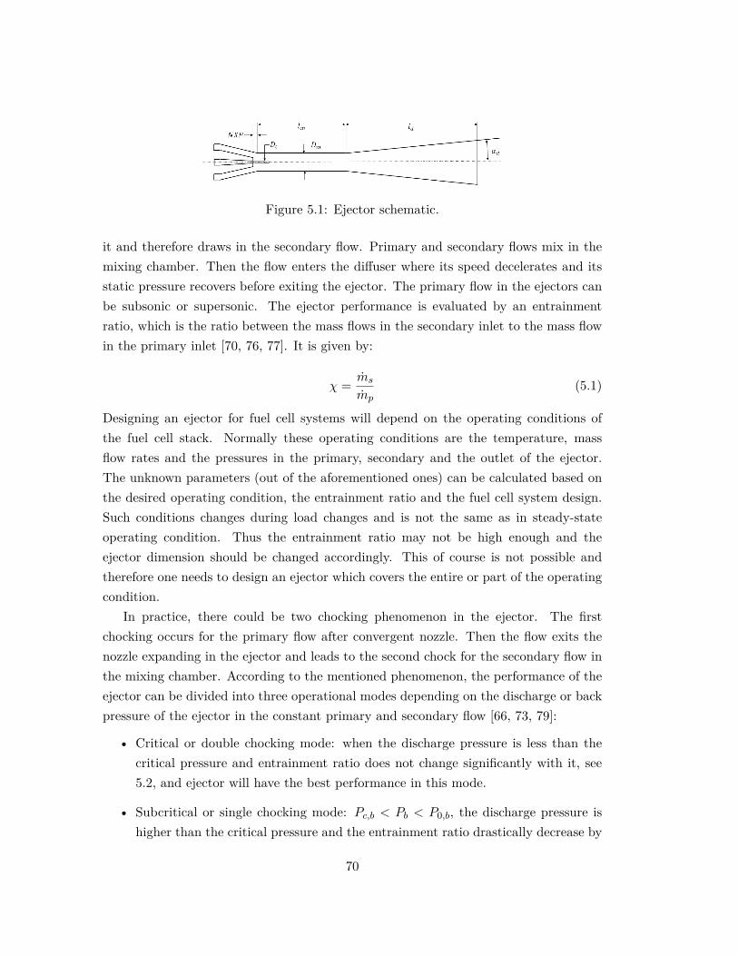
Figure 5.1: Ejector schematic.

it and therefore draws in the secondary flow. Primary and secondary flows mix in themixing chamber. Then the flow enters the diffuser where its speed decelerates and itsstatic pressure recovers before exiting the ejector. The primary flow in the ejectors canbe subsonic or supersonic. The ejector performance is evaluated by an entrainmentratio, which is the ratio between the mass flows in the secondary inlet to the mass flowin the primary inlet [70, 76, 77]. It is given by:

χ = ms

mp(5.1)

Designing an ejector for fuel cell systems will depend on the operating conditions ofthe fuel cell stack. Normally these operating conditions are the temperature, massflow rates and the pressures in the primary, secondary and the outlet of the ejector.The unknown parameters (out of the aforementioned ones) can be calculated based onthe desired operating condition, the entrainment ratio and the fuel cell system design.Such conditions changes during load changes and is not the same as in steady-stateoperating condition. Thus the entrainment ratio may not be high enough and theejector dimension should be changed accordingly. This of course is not possible andtherefore one needs to design an ejector which covers the entire or part of the operatingcondition.

In practice, there could be two chocking phenomenon in the ejector. The firstchocking occurs for the primary flow after convergent nozzle. Then the flow exits thenozzle expanding in the ejector and leads to the second chock for the secondary flow inthe mixing chamber. According to the mentioned phenomenon, the performance of theejector can be divided into three operational modes depending on the discharge or backpressure of the ejector in the constant primary and secondary flow [66, 73, 79]:

• Critical or double chocking mode: when the discharge pressure is less than thecritical pressure and entrainment ratio does not change significantly with it, see5.2, and ejector will have the best performance in this mode.

• Subcritical or single chocking mode: Pc,b < Pb < P0,b, the discharge pressure ishigher than the critical pressure and the entrainment ratio drastically decrease by

70

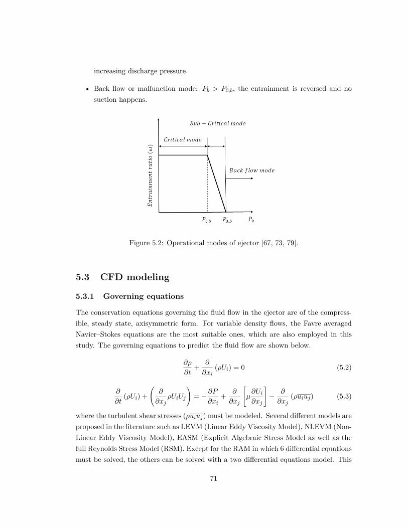
increasing discharge pressure.

• Back flow or malfunction mode: Pb > P0,b, the entrainment is reversed and nosuction happens.

Figure 5.2: Operational modes of ejector [67, 73, 79].

5.3 CFD modeling

5.3.1 Governing equations

The conservation equations governing the fluid flow in the ejector are of the compress-ible, steady state, axisymmetric form. For variable density flows, the Favre averagedNavier–Stokes equations are the most suitable ones, which are also employed in thisstudy. The governing equations to predict the fluid flow are shown below.

∂ρ

∂t+ ∂

∂xi(ρUi) = 0 (5.2)

∂

∂t(ρUi) +

(∂

∂xjρUiUj

)= − ∂P

∂xi+ ∂

∂xj

[µ∂Ui∂xj

]− ∂

∂xj(ρuiuj) (5.3)

where the turbulent shear stresses (ρuiuj) must be modeled. Several different models areproposed in the literature such as LEVM (Linear Eddy Viscosity Model), NLEVM (Non-Linear Eddy Viscosity Model), EASM (Explicit Algebraic Stress Model as well as thefull Reynolds Stress Model (RSM). Except for the RAM in which 6 differential equationsmust be solved, the others can be solved with a two differential equations model. This

71

means that the RSM modeling requires substantial larger calculation time comparedto the two-equation models. Due to 2D nature of the calculation and availability inANSYS program the simplest for which is the LEVM is used in this study.

ρuiuj = 23ρkσij − µt

(∂Ui∂xj

+ ∂Uj∂xi

)(5.4)

which originates from Boussinesq approximation of the eddy viscosity. This means thatat all points of a turbulent flow, the principal axes of the Reynolds stresses are coincidingwith those of the mean strain rate tensor (isotropy assumption). Assuming ideal gasthe density can be calculated from:

ρ = P

RT(5.5)

Several two-equations model are proposed in the literature such as k−ε, k−τ and k−ω,where k is the kinetic energy, ε is the dissipation rate, τ is the turbulent time-scale andω is the reciprocal turbulent time-scale (or specific dissipation). In the regions of lowturbulence where both k and ε approach zero, large numerical problems may arise inthe ε - equation as k becomes zero, see e.g. [81]. Both must go to zero in a correctrate to avoid the problem, which is often not the case. Therefore a damping functionmust be introduced to avoid the problem. Alternatively, the small scales of turbulenceshall be removed systematically to a point where the large scales are resolvable whichis called as Re-Normalization Group or RNG k − ε . Such a problem does not appearin the ω - equation, which is also the main reason why this model is used in this study.The shear stress transport (SST) k – ω of model of [82] is used here, as shown below:

∂

∂t(ρk) + ∂

∂xj(Uj (ρk + P )) = ∂

∂xj

[(µ+ µt

σk

)∂k

∂xj

]− ρuiuj

∂Ui∂xj− kω (5.6)

∂

∂t(ρω) + ∂

∂xj(ρUjω) = ∂

∂xj

[(µ+ µt

σω

)∂ω

∂xj

]+ Cω1

ω

kρuiuj

∂Ui∂xj− Cω2ρω

2 (5.7)

In order to avoid the numerical stiffness which may arise in some local point, the tur-bulent viscosity is limited by introducing a damping function and avoiding its value toexceed the local strain rate of turbulence

72

µτ = ρk

ω

1max

[1α∗ ,

SF2α1ω

] (5.8)

where S is the strain rate magnitude given by

S = 2√SijSij Sij = 1

2

(∂Uj∂xi

+ ∂Ui∂xj

)(5.9)

and the turbulent Prandtl numbers for k and ω are defined as

σk = 1F!σk1

+ 1−F!σk2

σω = 1F!σω1

+ 1−F!σω2

(5.10)

The damping coefficient for turbulent viscosity is defined as

α∗ = 0.024 +Ret/61 +Ret/6

(5.11)

The local turbulent Re-number is

Ret = ρk

µω(5.12)

and the blending functions F1 is given by

F1 = tanh(φ

41

)(5.13)

φ1 = min

[max

( √k

0.09ωy ,500µρωy2

),

4ρkσw2D

+wy

2

](5.14)

D+ω = max

[2ρ 1σω2ω

∂k

∂xj

∂ω

∂xj, 10−10

](5.15)

while the blending function F2 is defined as

F2 = tanh(φ

22

)(5.16)

φ2 = max

[2√k

0.09ωy ,500µρωy2

](5.17)

Model constants are Cω1 = 5/9, Cω2 = 5/6, σω1 = 2.0, σω” = 1.168, σk1 = 0.176 andσk2 = 1.0. In the above equations ρ is the density, µ is the laminar viscosity and y isthe normal distance to the nearest wall.

73

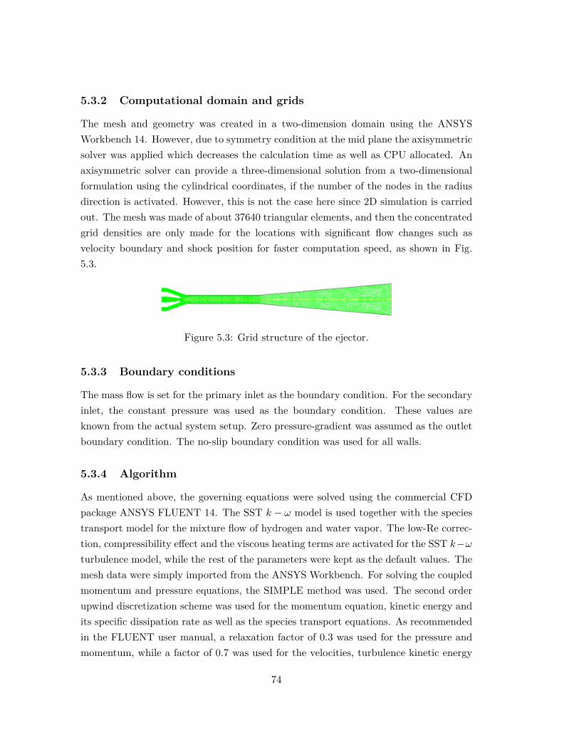
5.3.2 Computational domain and grids

The mesh and geometry was created in a two-dimension domain using the ANSYSWorkbench 14. However, due to symmetry condition at the mid plane the axisymmetricsolver was applied which decreases the calculation time as well as CPU allocated. Anaxisymmetric solver can provide a three-dimensional solution from a two-dimensionalformulation using the cylindrical coordinates, if the number of the nodes in the radiusdirection is activated. However, this is not the case here since 2D simulation is carriedout. The mesh was made of about 37640 triangular elements, and then the concentratedgrid densities are only made for the locations with significant flow changes such asvelocity boundary and shock position for faster computation speed, as shown in Fig.5.3.

Figure 5.3: Grid structure of the ejector.

5.3.3 Boundary conditions

The mass flow is set for the primary inlet as the boundary condition. For the secondaryinlet, the constant pressure was used as the boundary condition. These values areknown from the actual system setup. Zero pressure-gradient was assumed as the outletboundary condition. The no-slip boundary condition was used for all walls.

5.3.4 Algorithm

As mentioned above, the governing equations were solved using the commercial CFDpackage ANSYS FLUENT 14. The SST k − ω model is used together with the speciestransport model for the mixture flow of hydrogen and water vapor. The low-Re correc-tion, compressibility effect and the viscous heating terms are activated for the SST k−ωturbulence model, while the rest of the parameters were kept as the default values. Themesh data were simply imported from the ANSYS Workbench. For solving the coupledmomentum and pressure equations, the SIMPLE method was used. The second orderupwind discretization scheme was used for the momentum equation, kinetic energy andits specific dissipation rate as well as the species transport equations. As recommendedin the FLUENT user manual, a relaxation factor of 0.3 was used for the pressure andmomentum, while a factor of 0.7 was used for the velocities, turbulence kinetic energy

74

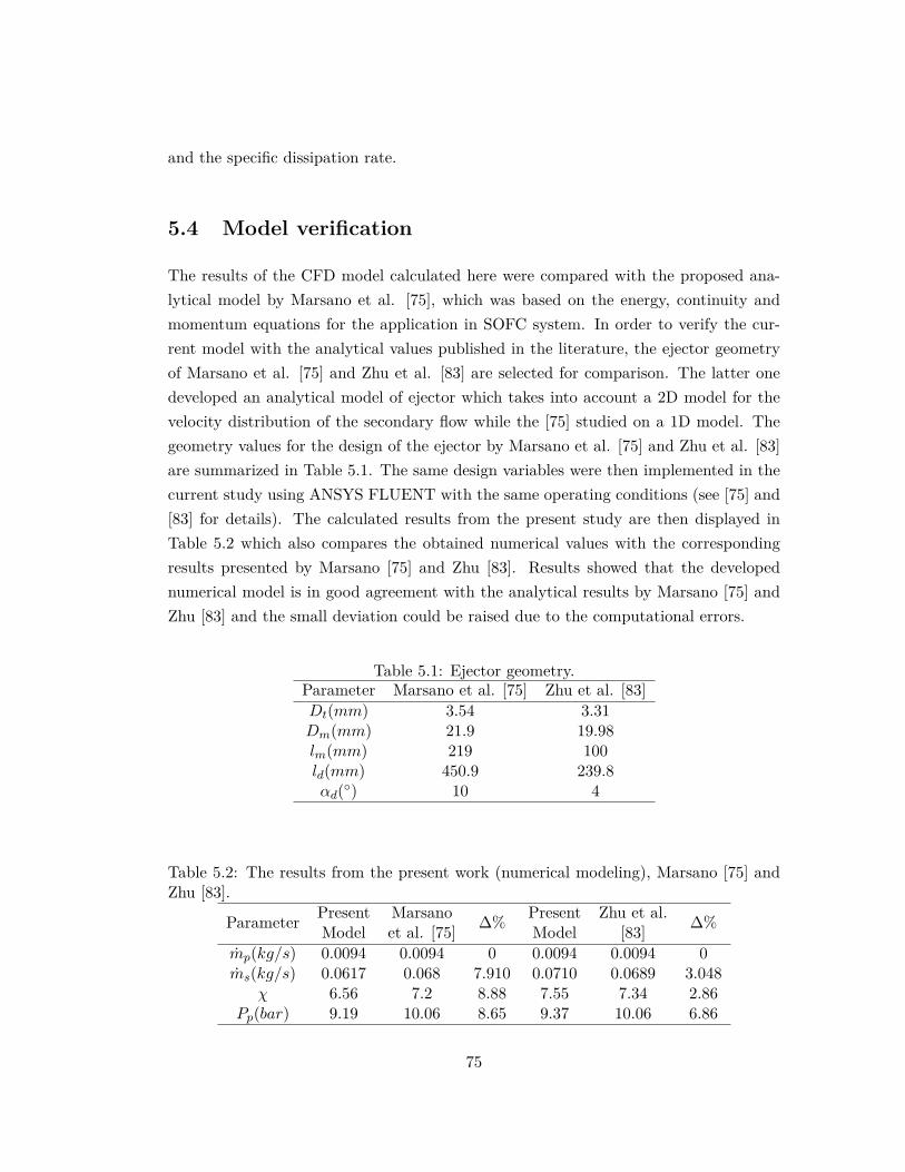
and the specific dissipation rate.

5.4 Model verification

The results of the CFD model calculated here were compared with the proposed ana-lytical model by Marsano et al. [75], which was based on the energy, continuity andmomentum equations for the application in SOFC system. In order to verify the cur-rent model with the analytical values published in the literature, the ejector geometryof Marsano et al. [75] and Zhu et al. [83] are selected for comparison. The latter onedeveloped an analytical model of ejector which takes into account a 2D model for thevelocity distribution of the secondary flow while the [75] studied on a 1D model. Thegeometry values for the design of the ejector by Marsano et al. [75] and Zhu et al. [83]are summarized in Table 5.1. The same design variables were then implemented in thecurrent study using ANSYS FLUENT with the same operating conditions (see [75] and[83] for details). The calculated results from the present study are then displayed inTable 5.2 which also compares the obtained numerical values with the correspondingresults presented by Marsano [75] and Zhu [83]. Results showed that the developednumerical model is in good agreement with the analytical results by Marsano [75] andZhu [83] and the small deviation could be raised due to the computational errors.

Table 5.1: Ejector geometry.Parameter Marsano et al. [75] Zhu et al. [83]Dt(mm) 3.54 3.31Dm(mm) 21.9 19.98lm(mm) 219 100ld(mm) 450.9 239.8αd() 10 4

Table 5.2: The results from the present work (numerical modeling), Marsano [75] andZhu [83].

Parameter Present Marsano ∆% Present Zhu et al. ∆%Model et al. [75] Model [83]mp(kg/s) 0.0094 0.0094 0 0.0094 0.0094 0ms(kg/s) 0.0617 0.068 7.910 0.0710 0.0689 3.048

χ 6.56 7.2 8.88 7.55 7.34 2.86Pp(bar) 9.19 10.06 8.65 9.37 10.06 6.86

75

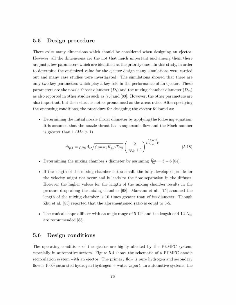
5.5 Design procedure

There exist many dimensions which should be considered when designing an ejector.However, all the dimensions are the not that much important and among them thereare just a few parameters which are identified as the priority ones. In this study, in orderto determine the optimized value for the ejector design many simulations were carriedout and many case studies were investigated. The simulations showed that there areonly two key parameters which play a key role in the performance of an ejector. Theseparameters are the nozzle throat diameter (Dt) and the mixing chamber diameter (Dm)as also reported in other studies such as [73] and [83]. However, the other parameters arealso important, but their effect is not as pronounced as the areas ratio. After specifyingthe operating conditions, the procedure for designing the ejector followed as:

• Determining the initial nozzle throat diameter by applying the following equation.It is assumed that the nozzle throat has a supersonic flow and the Mach numberis greater than 1 (Ma > 1).

mp,1 = ρP,0At√ψPκP,0Rg,PTP,0

(2

κP,0 + 1

) κP,0+12(κP,0−1)

(5.18)

• Determining the mixing chamber’s diameter by assuming DmDt

= 3− 6 [84].

• If the length of the mixing chamber is too small, the fully developed profile forthe velocity might not occur and it leads to the flow separation in the diffuser.However the higher values for the length of the mixing chamber results in thepressure drop along the mixing chamber [68]. Marsano et al. [75] assumed thelength of the mixing chamber is 10 times greater than of its diameter. ThoughZhu et al. [83] reported that the aforementioned ratio is equal to 3-5.

• The conical shape diffuser with an angle range of 5-12 and the length of 4-12 Dm

are recommended [83].

5.6 Design conditions

The operating conditions of the ejector are highly affected by the PEMFC system,especially in automotive sectors. Figure 5.4 shows the schematic of a PEMFC anodicrecirculation system with an ejector. The primary flow is pure hydrogen and secondaryflow is 100% saturated hydrogen (hydrogen + water vapor). In automotive systems, the

76

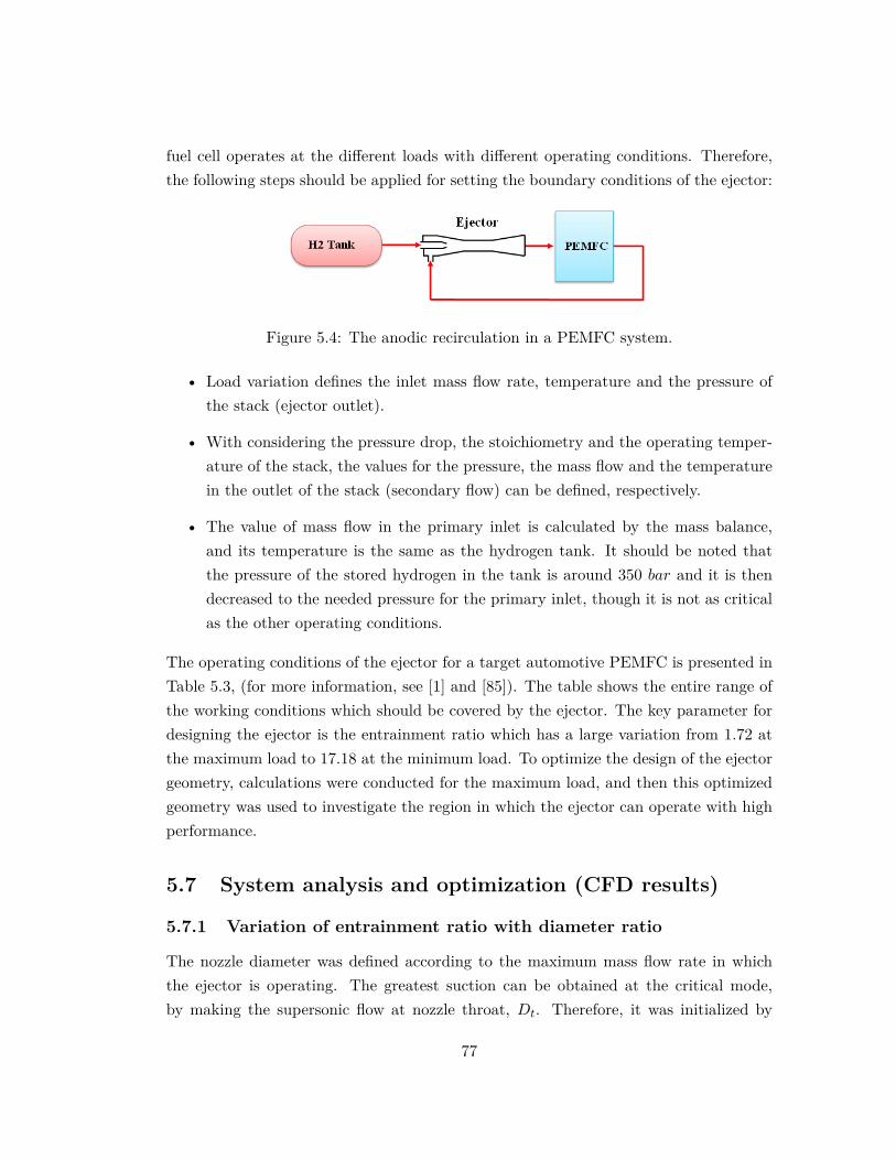
fuel cell operates at the different loads with different operating conditions. Therefore,the following steps should be applied for setting the boundary conditions of the ejector:

Figure 5.4: The anodic recirculation in a PEMFC system.

• Load variation defines the inlet mass flow rate, temperature and the pressure ofthe stack (ejector outlet).

• With considering the pressure drop, the stoichiometry and the operating temper-ature of the stack, the values for the pressure, the mass flow and the temperaturein the outlet of the stack (secondary flow) can be defined, respectively.

• The value of mass flow in the primary inlet is calculated by the mass balance,and its temperature is the same as the hydrogen tank. It should be noted thatthe pressure of the stored hydrogen in the tank is around 350 bar and it is thendecreased to the needed pressure for the primary inlet, though it is not as criticalas the other operating conditions.

The operating conditions of the ejector for a target automotive PEMFC is presented inTable 5.3, (for more information, see [1] and [85]). The table shows the entire range ofthe working conditions which should be covered by the ejector. The key parameter fordesigning the ejector is the entrainment ratio which has a large variation from 1.72 atthe maximum load to 17.18 at the minimum load. To optimize the design of the ejectorgeometry, calculations were conducted for the maximum load, and then this optimizedgeometry was used to investigate the region in which the ejector can operate with highperformance.

5.7 System analysis and optimization (CFD results)

5.7.1 Variation of entrainment ratio with diameter ratio

The nozzle diameter was defined according to the maximum mass flow rate in whichthe ejector is operating. The greatest suction can be obtained at the critical mode,by making the supersonic flow at nozzle throat, Dt. Therefore, it was initialized by

77

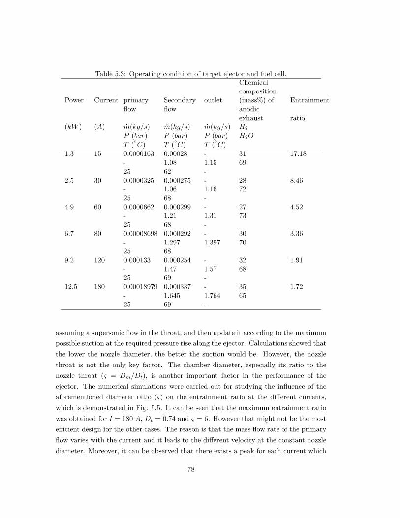
Table 5.3: Operating condition of target ejector and fuel cell.Chemicalcomposition

Power Current primaryflow

Secondaryflow

outlet (mass%) ofanodic

Entrainment

exhaust ratio(kW ) (A) m(kg/s) m(kg/s) m(kg/s) H2

P (bar) P (bar) P (bar) H2OT (

C) T (C) T (

C)1.3 15 0.0000163 0.00028 - 31 17.18

- 1.08 1.15 6925 62 -

2.5 30 0.0000325 0.000275 - 28 8.46- 1.06 1.16 7225 68 -

4.9 60 0.0000662 0.000299 - 27 4.52- 1.21 1.31 7325 68 -

6.7 80 0.00008698 0.000292 - 30 3.36- 1.297 1.397 7025 68

9.2 120 0.000133 0.000254 - 32 1.91- 1.47 1.57 6825 69 -

12.5 180 0.00018979 0.000337 - 35 1.72- 1.645 1.764 6525 69 -

assuming a supersonic flow in the throat, and then update it according to the maximumpossible suction at the required pressure rise along the ejector. Calculations showed thatthe lower the nozzle diameter, the better the suction would be. However, the nozzlethroat is not the only key factor. The chamber diameter, especially its ratio to thenozzle throat (ς = Dm/Dt), is another important factor in the performance of theejector. The numerical simulations were carried out for studying the influence of theaforementioned diameter ratio (ς) on the entrainment ratio at the different currents,which is demonstrated in Fig. 5.5. It can be seen that the maximum entrainment ratiowas obtained for I = 180 A, Dt = 0.74 and ς = 6. However that might not be the mostefficient design for the other cases. The reason is that the mass flow rate of the primaryflow varies with the current and it leads to the different velocity at the constant nozzlediameter. Moreover, it can be observed that there exists a peak for each current which

78

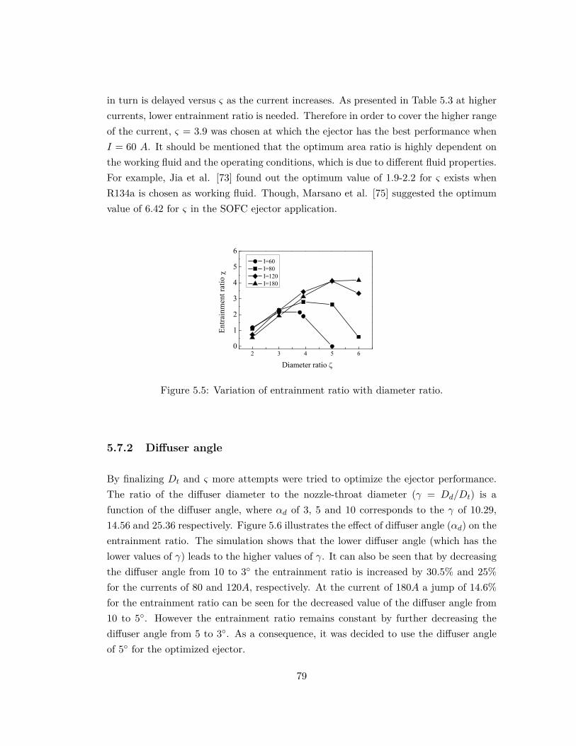
in turn is delayed versus ς as the current increases. As presented in Table 5.3 at highercurrents, lower entrainment ratio is needed. Therefore in order to cover the higher rangeof the current, ς = 3.9 was chosen at which the ejector has the best performance whenI = 60 A. It should be mentioned that the optimum area ratio is highly dependent onthe working fluid and the operating conditions, which is due to different fluid properties.For example, Jia et al. [73] found out the optimum value of 1.9-2.2 for ς exists whenR134a is chosen as working fluid. Though, Marsano et al. [75] suggested the optimumvalue of 6.42 for ς in the SOFC ejector application.

2 3 4 5 60

1

2

3

4

5

6

Entra

inm

ent r

atio

Diameter ratio

I=60 I=80 I=120 I=180

Figure 5.5: Variation of entrainment ratio with diameter ratio.

5.7.2 Diffuser angle

By finalizing Dt and ς more attempts were tried to optimize the ejector performance.The ratio of the diffuser diameter to the nozzle-throat diameter (γ = Dd/Dt) is afunction of the diffuser angle, where αd of 3, 5 and 10 corresponds to the γ of 10.29,14.56 and 25.36 respectively. Figure 5.6 illustrates the effect of diffuser angle (αd) on theentrainment ratio. The simulation shows that the lower diffuser angle (which has thelower values of γ) leads to the higher values of γ. It can also be seen that by decreasingthe diffuser angle from 10 to 3 the entrainment ratio is increased by 30.5% and 25%for the currents of 80 and 120A, respectively. At the current of 180A a jump of 14.6%for the entrainment ratio can be seen for the decreased value of the diffuser angle from10 to 5. However the entrainment ratio remains constant by further decreasing thediffuser angle from 5 to 3. As a consequence, it was decided to use the diffuser angleof 5 for the optimized ejector.

79

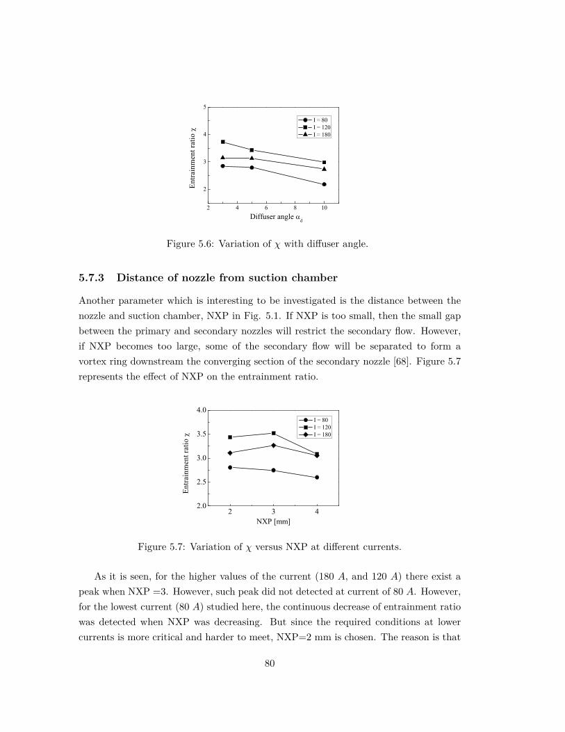
2 4 6 8 10

2

3

4

5

Entra

inm

ent r

atio

Diffuser angle d

I = 80 I = 120 I = 180

Figure 5.6: Variation of χ with diffuser angle.

5.7.3 Distance of nozzle from suction chamber

Another parameter which is interesting to be investigated is the distance between thenozzle and suction chamber, NXP in Fig. 5.1. If NXP is too small, then the small gapbetween the primary and secondary nozzles will restrict the secondary flow. However,if NXP becomes too large, some of the secondary flow will be separated to form avortex ring downstream the converging section of the secondary nozzle [68]. Figure 5.7represents the effect of NXP on the entrainment ratio.

2 3 42.0

2.5

3.0

3.5

4.0

Entra

inm

ent r

atio

NXP [mm]

I = 80 I = 120 I = 180

Figure 5.7: Variation of χ versus NXP at different currents.

As it is seen, for the higher values of the current (180 A, and 120 A) there exist apeak when NXP =3. However, such peak did not detected at current of 80 A. However,for the lowest current (80 A) studied here, the continuous decrease of entrainment ratiowas detected when NXP was decreasing. But since the required conditions at lowercurrents is more critical and harder to meet, NXP=2 mm is chosen. The reason is that

80

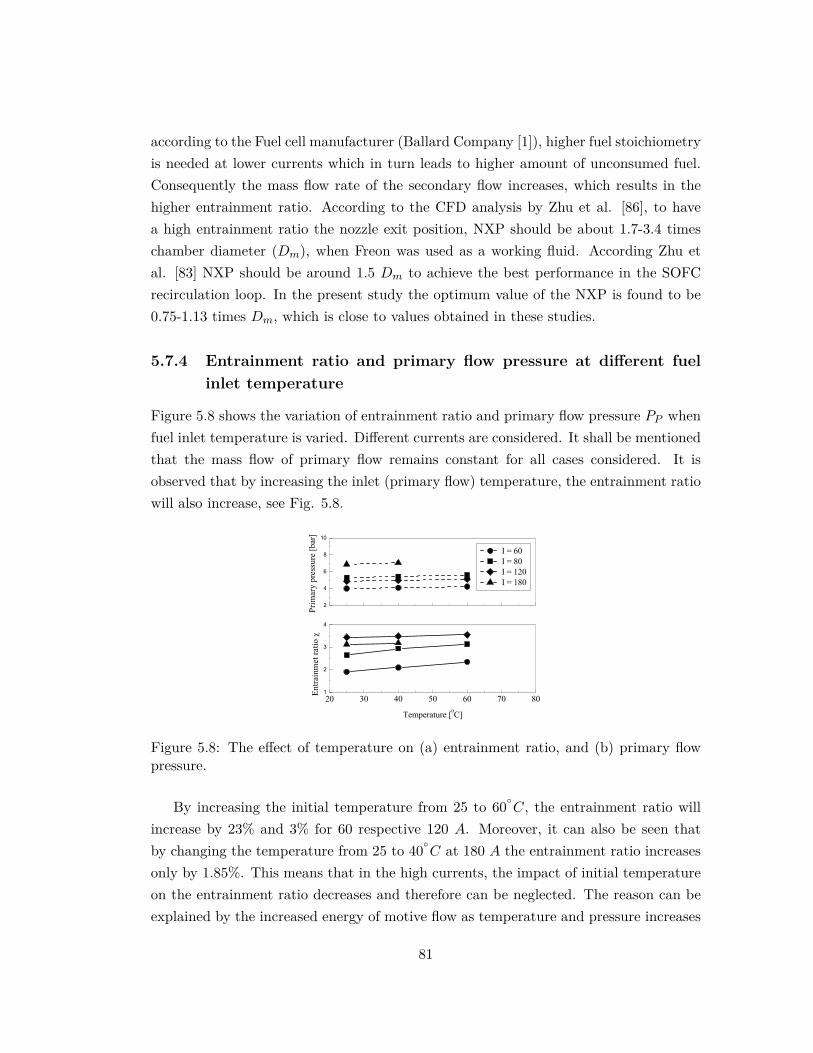
according to the Fuel cell manufacturer (Ballard Company [1]), higher fuel stoichiometryis needed at lower currents which in turn leads to higher amount of unconsumed fuel.Consequently the mass flow rate of the secondary flow increases, which results in thehigher entrainment ratio. According to the CFD analysis by Zhu et al. [86], to havea high entrainment ratio the nozzle exit position, NXP should be about 1.7-3.4 timeschamber diameter (Dm), when Freon was used as a working fluid. According Zhu etal. [83] NXP should be around 1.5 Dm to achieve the best performance in the SOFCrecirculation loop. In the present study the optimum value of the NXP is found to be0.75-1.13 times Dm, which is close to values obtained in these studies.

5.7.4 Entrainment ratio and primary flow pressure at different fuelinlet temperature

Figure 5.8 shows the variation of entrainment ratio and primary flow pressure PP whenfuel inlet temperature is varied. Different currents are considered. It shall be mentionedthat the mass flow of primary flow remains constant for all cases considered. It isobserved that by increasing the inlet (primary flow) temperature, the entrainment ratiowill also increase, see Fig. 5.8.

20 30 40 50 60 70 801

2

3

4

Entra

inm

et ra

tio

Temperature [0C]

2

4

6

8

10

I = 60 I = 80 I = 120 I = 180

Prim

ary

pres

sure

[bar

]

Figure 5.8: The effect of temperature on (a) entrainment ratio, and (b) primary flowpressure.

By increasing the initial temperature from 25 to 60C, the entrainment ratio will

increase by 23% and 3% for 60 respective 120 A. Moreover, it can also be seen thatby changing the temperature from 25 to 40

C at 180 A the entrainment ratio increasesonly by 1.85%. This means that in the high currents, the impact of initial temperatureon the entrainment ratio decreases and therefore can be neglected. The reason can beexplained by the increased energy of motive flow as temperature and pressure increases

81

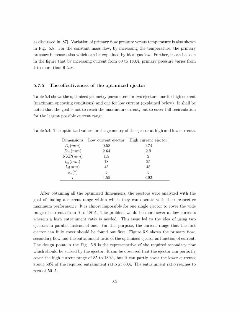
as discussed in [87]. Variation of primary flow pressure versus temperature is also shownin Fig. 5.8. For the constant mass flow, by increasing the temperature, the primarypressure increases also which can be explained by ideal gas law. Further, it can be seenin the figure that by increasing current from 60 to 180A, primary pressure varies from4 to more than 6 bar.

5.7.5 The effectiveness of the optimized ejector

Table 5.4 shows the optimized geometry parameters for two ejectors; one for high current(maximum operating conditions) and one for low current (explained below). It shall benoted that the goal is not to reach the maximum current, but to cover full recirculationfor the largest possible current range.

Table 5.4: The optimized values for the geometry of the ejector at high and low currents.

Dimensions Low current ejector High current ejectorDt(mm) 0.58 0.74Dm(mm) 2.64 2.9NXP(mm) 1.5 2lm(mm) 18 25ld(mm) 45 45αd() 3 5ς 4.55 3.92

After obtaining all the optimized dimensions, the ejectors were analyzed with thegoal of finding a current range within which they can operate with their respectivemaximum performance. It is almost impossible for one single ejector to cover the widerange of currents from 0 to 180A. The problem would be more sever at low currentswherein a high entrainment ratio is needed. This issue led to the idea of using twoejectors in parallel instead of one. For this purpose, the current range that the firstejector can fully cover should be found out first. Figure 5.9 shows the primary flow,secondary flow and the entrainment ratio of the optimized ejector as function of current.The design point in the Fig. 5.9 is the representative of the required secondary flowwhich should be sucked by the ejector. It can be observed that the ejector can perfectlycover the high current range of 85 to 180A, but it can partly cover the lower currents;about 50% of the required entrainment ratio at 60A. The entrainment ratio reaches tozero at 50 A.

82

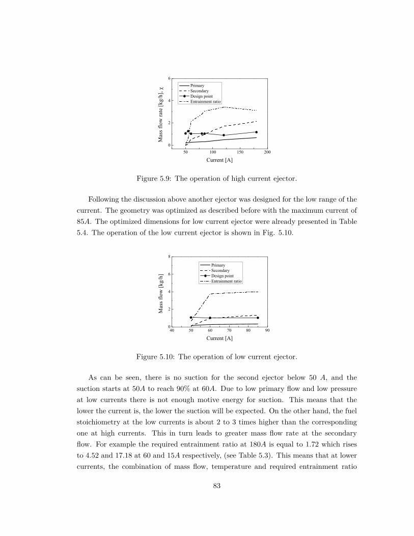
50 100 150 2000

2

4

6

Mas

s flo

w ra

te [k

g/h]

, Current [A]

Primary Secondary Design point Entrainment ratio

Figure 5.9: The operation of high current ejector.

Following the discussion above another ejector was designed for the low range of thecurrent. The geometry was optimized as described before with the maximum current of85A. The optimized dimensions for low current ejector were already presented in Table5.4. The operation of the low current ejector is shown in Fig. 5.10.

40 50 60 70 80 900

2

4

6

8

Mas

s flo

w [k

g/h]

Current [A]

Primary Secondary Design point Entrainment ratio

Figure 5.10: The operation of low current ejector.

As can be seen, there is no suction for the second ejector below 50 A, and thesuction starts at 50A to reach 90% at 60A. Due to low primary flow and low pressureat low currents there is not enough motive energy for suction. This means that thelower the current is, the lower the suction will be expected. On the other hand, the fuelstoichiometry at the low currents is about 2 to 3 times higher than the correspondingone at high currents. This in turn leads to greater mass flow rate at the secondaryflow. For example the required entrainment ratio at 180A is equal to 1.72 which risesto 4.52 and 17.18 at 60 and 15A respectively, (see Table 5.3). This means that at lowercurrents, the combination of mass flow, temperature and required entrainment ratio

83

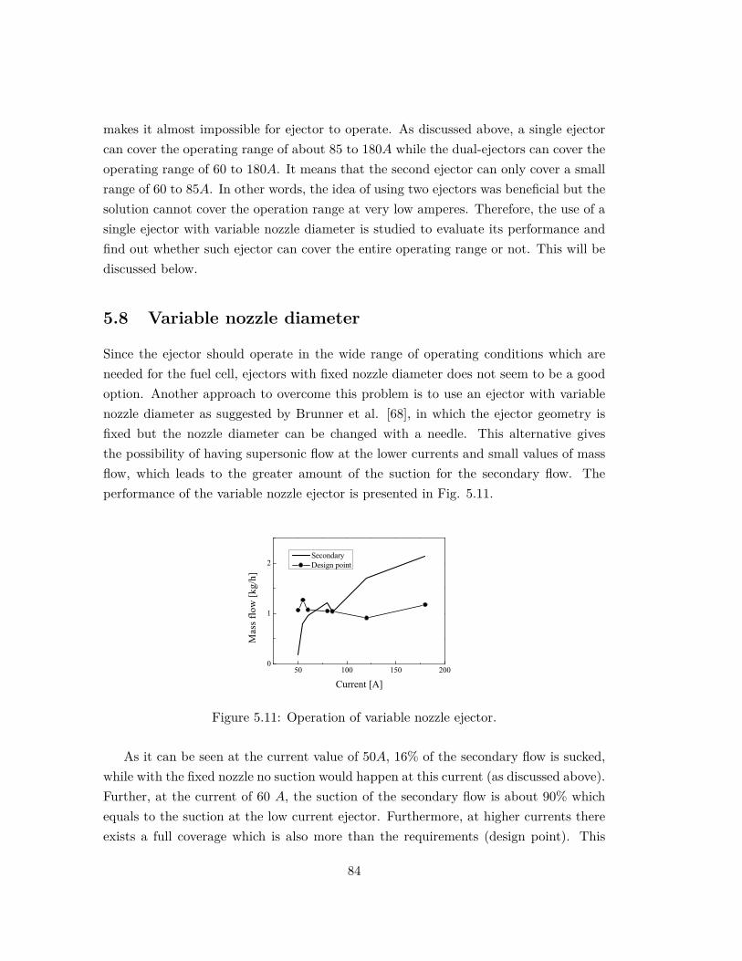
makes it almost impossible for ejector to operate. As discussed above, a single ejectorcan cover the operating range of about 85 to 180A while the dual-ejectors can cover theoperating range of 60 to 180A. It means that the second ejector can only cover a smallrange of 60 to 85A. In other words, the idea of using two ejectors was beneficial but thesolution cannot cover the operation range at very low amperes. Therefore, the use of asingle ejector with variable nozzle diameter is studied to evaluate its performance andfind out whether such ejector can cover the entire operating range or not. This will bediscussed below.

5.8 Variable nozzle diameter

Since the ejector should operate in the wide range of operating conditions which areneeded for the fuel cell, ejectors with fixed nozzle diameter does not seem to be a goodoption. Another approach to overcome this problem is to use an ejector with variablenozzle diameter as suggested by Brunner et al. [68], in which the ejector geometry isfixed but the nozzle diameter can be changed with a needle. This alternative givesthe possibility of having supersonic flow at the lower currents and small values of massflow, which leads to the greater amount of the suction for the secondary flow. Theperformance of the variable nozzle ejector is presented in Fig. 5.11.

50 100 150 2000

1

2

Mas

s flo

w [k

g/h]

Current [A]

Secondary Design point

Figure 5.11: Operation of variable nozzle ejector.

As it can be seen at the current value of 50A, 16% of the secondary flow is sucked,while with the fixed nozzle no suction would happen at this current (as discussed above).Further, at the current of 60 A, the suction of the secondary flow is about 90% whichequals to the suction at the low current ejector. Furthermore, at higher currents thereexists a full coverage which is also more than the requirements (design point). This

84

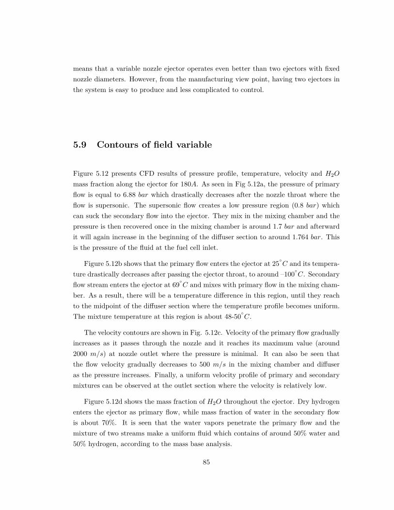
means that a variable nozzle ejector operates even better than two ejectors with fixednozzle diameters. However, from the manufacturing view point, having two ejectors inthe system is easy to produce and less complicated to control.

5.9 Contours of field variable

Figure 5.12 presents CFD results of pressure profile, temperature, velocity and H2O

mass fraction along the ejector for 180A. As seen in Fig 5.12a, the pressure of primaryflow is equal to 6.88 bar which drastically decreases after the nozzle throat where theflow is supersonic. The supersonic flow creates a low pressure region (0.8 bar) whichcan suck the secondary flow into the ejector. They mix in the mixing chamber and thepressure is then recovered once in the mixing chamber is around 1.7 bar and afterwardit will again increase in the beginning of the diffuser section to around 1.764 bar. Thisis the pressure of the fluid at the fuel cell inlet.

Figure 5.12b shows that the primary flow enters the ejector at 25C and its tempera-

ture drastically decreases after passing the ejector throat, to around –100C. Secondary

flow stream enters the ejector at 69C and mixes with primary flow in the mixing cham-

ber. As a result, there will be a temperature difference in this region, until they reachto the midpoint of the diffuser section where the temperature profile becomes uniform.The mixture temperature at this region is about 48-50

C.

The velocity contours are shown in Fig. 5.12c. Velocity of the primary flow graduallyincreases as it passes through the nozzle and it reaches its maximum value (around2000 m/s) at nozzle outlet where the pressure is minimal. It can also be seen thatthe flow velocity gradually decreases to 500 m/s in the mixing chamber and diffuseras the pressure increases. Finally, a uniform velocity profile of primary and secondarymixtures can be observed at the outlet section where the velocity is relatively low.

Figure 5.12d shows the mass fraction of H2O throughout the ejector. Dry hydrogenenters the ejector as primary flow, while mass fraction of water in the secondary flowis about 70%. It is seen that the water vapors penetrate the primary flow and themixture of two streams make a uniform fluid which contains of around 50% water and50% hydrogen, according to the mass base analysis.

85

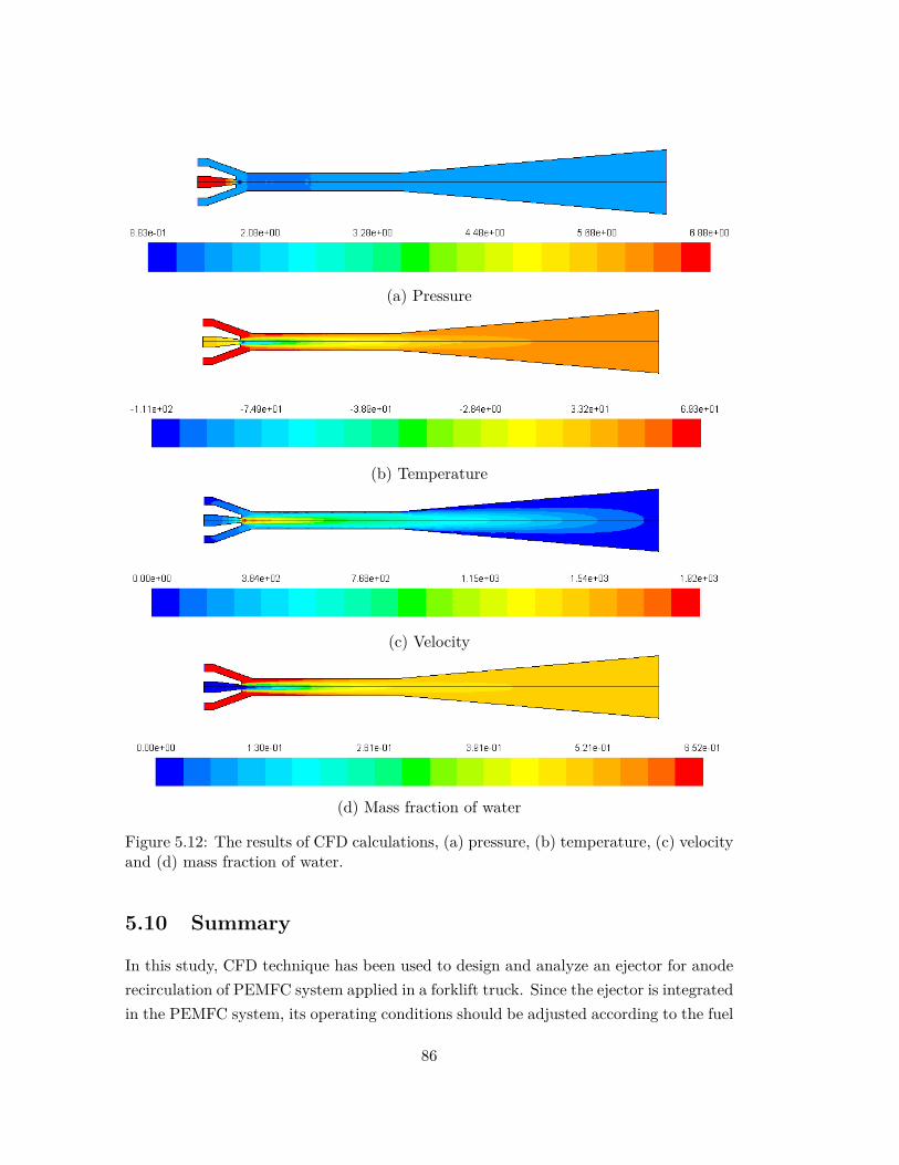
(a) Pressure

(b) Temperature

(c) Velocity

(d) Mass fraction of water

Figure 5.12: The results of CFD calculations, (a) pressure, (b) temperature, (c) velocityand (d) mass fraction of water.

5.10 Summary

In this study, CFD technique has been used to design and analyze an ejector for anoderecirculation of PEMFC system applied in a forklift truck. Since the ejector is integratedin the PEMFC system, its operating conditions should be adjusted according to the fuel

86

cell load fluctuations to cover the current variation of the stack from 0-180 A. In orderfor the ejector to operate in the largest possible range of load, different approaches (withfixed nozzle and variable nozzle ejectors) have been investigated. For the first approachan ejector has been designed so that it could operate at the maximum load and mass flowrate. Then different geometries have been investigated in order to optimize the ejector.The optimization is carried out not only by considering the best performance of ejectorat maximum load with operation in the larger range as priority, but also catching thedesign point at maximum load even though it does not have the best efficiency at suchpoint. The geometry analysis showed that diameter ratios (ς) is the key parameter indesigning the ejector, and by choosing ς = 3.9 at Dt = 0.74 the ejector can operate from85-180A properly. However, in order to increase the operating range, another ejectorwas designed for maximum current of 85A. By optimization the second ejector it wasfound that it could operate 100% at 85A and down to 90% at 60A. The third approachwas applying an ejector with variable nozzle diameter. The results showed that suchejector con also operate 100% at 180A down to 90% at 60A. However, in practice itis more difficult to manufacture an ejector with variable nozzle compared to an ejectorwith the fixed nozzle diameter, but it could be the best choice for having the greatestentrainment ratio in the system.

87

Chapter 6

Performance simulation andanalysis of a fuel cell / batteryhybrid forklift truck

6.1 overview

Fuel cells can be implemented in automotive power trains either as standalone systemsor in combination with other power sources such as a battery or an ultra-capacitorto create a hybrid system. Such hybrid systems exhibit distinct advantages such asthe ability to downsize the stack which in turn decreases the fuel cell cost, and alsoisolating the fuel cell from load fluctuations which promotes stack lifetime. In addi-tion, hybridization can improve fuel economy by exploiting regenerative power from thetraction motor while braking. Such hybrid power trains are particularly well suited fortransit applications where the average power demand is low due to frequent starts andstops of the vehicle [88]. The fuel economy of a hybrid vehicle is determined by theoverall size and weight of the vehicle, design of the hybrid platform, energy managementstrategy, driving conditions, etc. [89]. According to [90] an advanced control strategy isnecessary to achieve high fuel economy and good drivability. The literature reveals thatprevious efforts have focused either on the design and modeling of the stack itself, or onthe incorporation of the stack into the system to investigate its behavior as a function ofcontrol strategy and operating conditions. For example, [91] examined the requirementsof a fuel cell system that could be implemented on a wide range of cars. They conducted

88

simulations to investigate the transient response of the system (fuel cell and compressor)in order to optimize system start-up. Similarly, in [16] a 120 kW PEMFC and its sub-systems were modeled and validated against experimental data. In [92] different hybriddrive train configurations for fuel cell city buses were presented and the resulting energydistribution, hydrogen consumption, battery state-of-charge (SOC), and the power vari-ation rate were analyzed. Forklift propulsion systems and distributed power generationare identified as potential fuel cell applications for near-term markets. Replacement ofinternal combustion engine forklifts with either fuel-cell or battery-powered units offersthe potential to reduce the consumption of fossil fuels and petroleum imports [27], whilealso eliminating harmful emissions. The literature contains very few papers which haveaddressed hybrid fuel cell/battery forklift systems. In [26] two triple-hybrid systemsincluding a 16 kW fuel cell, battery, and ultra-capacitor were investigated for a forkliftsystem. Their simulations indicate that while a battery alone significantly reduces theload variations of the fuel cell, an ultra-capacitor reduces them even further. In thisstudy a simulation tool named LFM (Light, Fast and Modifiable), has been used toinvestigate the most efficient design for a forklift truck powered by a fuel cell/batteryhybrid. The study considers the effect of the size of the power sources, control strat-egy, and different operating conditions to optimize performance. The LFM simulationtool has been previously validated and employed for designing and optimizing hybridfuel cell buses at the University of Delaware [88], [93], and [94]. This study examinesimportant performance metrics such as hydrogen consumption and battery SOC as afunction of fuel cell and battery size, control strategy, drive cycle, and load variationfor a forklift truck system which has not been considered in previous studies.

6.2 Description of simulation tool and forklift truck sys-tem

6.2.1 LFM simulation tool

LFM is a component-based program which operates in Matlab/Simulink. The programconsists of various subsystems which are linked using electrical, mechanical, and controlsignals to construct a virtual vehicle. Models for all subsystems including the vehiclechassis, fuel cell, battery, motor, transmission, etc., are constructed within LFM usingtheir specifications and operating characteristics. LFM uses the desired drive cycle asan input in order to perform calculations by implementing a drive cycle-based, forward-facing model. At each time step, the LFM simulator calculates and compares the current

89

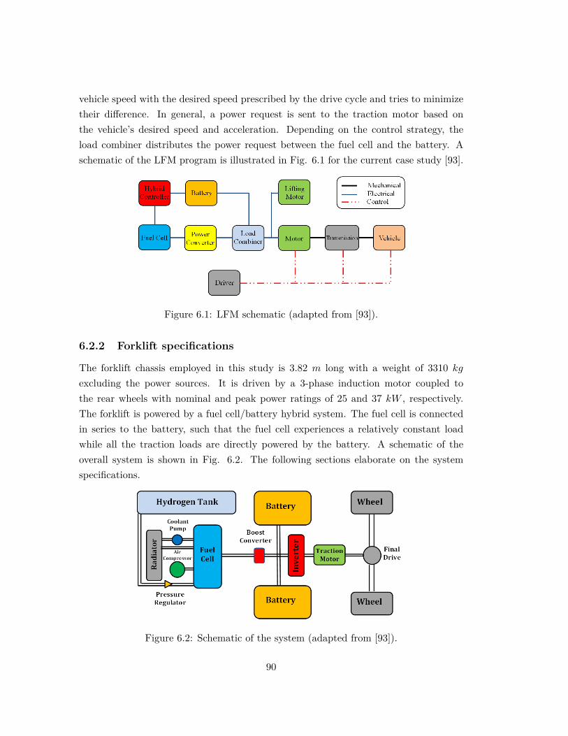
vehicle speed with the desired speed prescribed by the drive cycle and tries to minimizetheir difference. In general, a power request is sent to the traction motor based onthe vehicle’s desired speed and acceleration. Depending on the control strategy, theload combiner distributes the power request between the fuel cell and the battery. Aschematic of the LFM program is illustrated in Fig. 6.1 for the current case study [93].

Figure 6.1: LFM schematic (adapted from [93]).

6.2.2 Forklift specifications

The forklift chassis employed in this study is 3.82 m long with a weight of 3310 kgexcluding the power sources. It is driven by a 3-phase induction motor coupled tothe rear wheels with nominal and peak power ratings of 25 and 37 kW , respectively.The forklift is powered by a fuel cell/battery hybrid system. The fuel cell is connectedin series to the battery, such that the fuel cell experiences a relatively constant loadwhile all the traction loads are directly powered by the battery. A schematic of theoverall system is shown in Fig. 6.2. The following sections elaborate on the systemspecifications.

Figure 6.2: Schematic of the system (adapted from [93]).

90

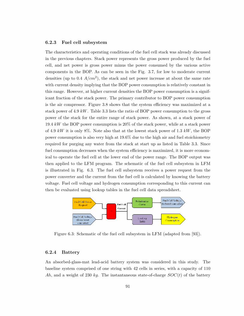
6.2.3 Fuel cell subsystem

The characteristics and operating conditions of the fuel cell stack was already discussedin the previous chapters. Stack power represents the gross power produced by the fuelcell, and net power is gross power minus the power consumed by the various activecomponents in the BOP. As can be seen in the Fig. 3.7, for low to moderate currentdensities (up to 0.4 A/cm2), the stack and net power increase at about the same ratewith current density implying that the BOP power consumption is relatively constant inthis range. However, at higher current densities the BOP power consumption is a signif-icant fraction of the stack power. The primary contributor to BOP power consumptionis the air compressor. Figure 3.8 shows that the system efficiency was maximized at astack power of 4.9 kW . Table 3.3 lists the ratio of BOP power consumption to the grosspower of the stack for the entire range of stack power. As shown, at a stack power of19.4 kW the BOP power consumption is 20% of the stack power, while at a stack powerof 4.9 kW it is only 8%. Note also that at the lowest stack power of 1.3 kW , the BOPpower consumption is also very high at 19.6% due to the high air and fuel stoichiometryrequired for purging any water from the stack at start up as listed in Table 3.3. Sincefuel consumption decreases when the system efficiency is maximized, it is more econom-ical to operate the fuel cell at the lower end of the power range. The BOP output wasthen applied to the LFM program. The schematic of the fuel cell subsystem in LFMis illustrated in Fig. 6.3. The fuel cell subsystem receives a power request from thepower converter and the current from the fuel cell is calculated by knowing the batteryvoltage. Fuel cell voltage and hydrogen consumption corresponding to this current canthen be evaluated using lookup tables in the fuel cell data spreadsheet.

Figure 6.3: Schematic of the fuel cell subsystem in LFM (adapted from [93]).

6.2.4 Battery

An absorbed-glass-mat lead-acid battery system was considered in this study. Thebaseline system comprised of one string with 42 cells in series, with a capacity of 110Ah, and a weight of 230 kg. The instantaneous state-of-charge SOC(t) of the battery

91

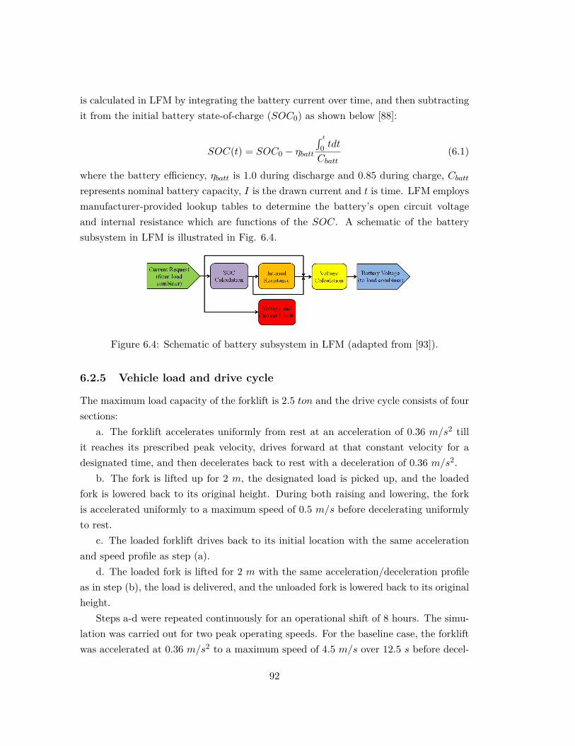
is calculated in LFM by integrating the battery current over time, and then subtractingit from the initial battery state-of-charge (SOC0) as shown below [88]:

SOC(t) = SOC0 − ηbatt´ t

0 tdt

Cbatt(6.1)

where the battery efficiency, ηbatt is 1.0 during discharge and 0.85 during charge, Cbattrepresents nominal battery capacity, I is the drawn current and t is time. LFM employsmanufacturer-provided lookup tables to determine the battery’s open circuit voltageand internal resistance which are functions of the SOC. A schematic of the batterysubsystem in LFM is illustrated in Fig. 6.4.

Figure 6.4: Schematic of battery subsystem in LFM (adapted from [93]).

6.2.5 Vehicle load and drive cycle

The maximum load capacity of the forklift is 2.5 ton and the drive cycle consists of foursections:

a. The forklift accelerates uniformly from rest at an acceleration of 0.36 m/s2 tillit reaches its prescribed peak velocity, drives forward at that constant velocity for adesignated time, and then decelerates back to rest with a deceleration of 0.36 m/s2.

b. The fork is lifted up for 2 m, the designated load is picked up, and the loadedfork is lowered back to its original height. During both raising and lowering, the forkis accelerated uniformly to a maximum speed of 0.5 m/s before decelerating uniformlyto rest.

c. The loaded forklift drives back to its initial location with the same accelerationand speed profile as step (a).

d. The loaded fork is lifted for 2 m with the same acceleration/deceleration profileas in step (b), the load is delivered, and the unloaded fork is lowered back to its originalheight.

Steps a-d were repeated continuously for an operational shift of 8 hours. The simu-lation was carried out for two peak operating speeds. For the baseline case, the forkliftwas accelerated at 0.36 m/s2 to a maximum speed of 4.5 m/s over 12.5 s before decel-

92

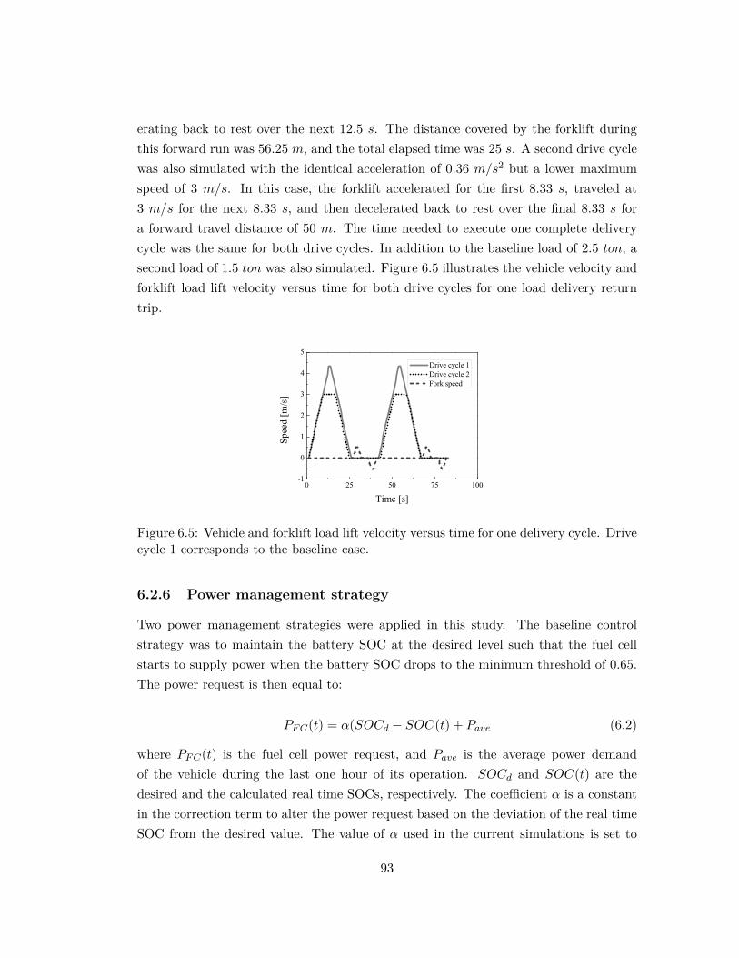
erating back to rest over the next 12.5 s. The distance covered by the forklift duringthis forward run was 56.25 m, and the total elapsed time was 25 s. A second drive cyclewas also simulated with the identical acceleration of 0.36 m/s2 but a lower maximumspeed of 3 m/s. In this case, the forklift accelerated for the first 8.33 s, traveled at3 m/s for the next 8.33 s, and then decelerated back to rest over the final 8.33 s fora forward travel distance of 50 m. The time needed to execute one complete deliverycycle was the same for both drive cycles. In addition to the baseline load of 2.5 ton, asecond load of 1.5 ton was also simulated. Figure 6.5 illustrates the vehicle velocity andforklift load lift velocity versus time for both drive cycles for one load delivery returntrip.

0 25 50 75 100-1

0

1

2

3

4

5

Spee

d [m

/s]

Time [s]

Drive cycle 1 Drive cycle 2 Fork speed

Figure 6.5: Vehicle and forklift load lift velocity versus time for one delivery cycle. Drivecycle 1 corresponds to the baseline case.

6.2.6 Power management strategy

Two power management strategies were applied in this study. The baseline controlstrategy was to maintain the battery SOC at the desired level such that the fuel cellstarts to supply power when the battery SOC drops to the minimum threshold of 0.65.The power request is then equal to:

PFC(t) = α(SOCd − SOC(t) + Pave (6.2)

where PFC(t) is the fuel cell power request, and Pave is the average power demandof the vehicle during the last one hour of its operation. SOCd and SOC(t) are thedesired and the calculated real time SOCs, respectively. The coefficient α is a constantin the correction term to alter the power request based on the deviation of the real timeSOC from the desired value. The value of α used in the current simulations is set to

93

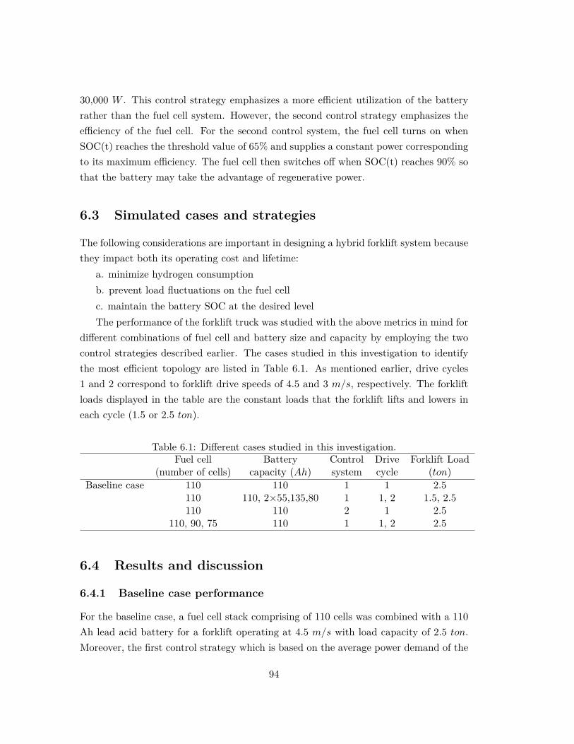
30,000 W . This control strategy emphasizes a more efficient utilization of the batteryrather than the fuel cell system. However, the second control strategy emphasizes theefficiency of the fuel cell. For the second control system, the fuel cell turns on whenSOC(t) reaches the threshold value of 65% and supplies a constant power correspondingto its maximum efficiency. The fuel cell then switches off when SOC(t) reaches 90% sothat the battery may take the advantage of regenerative power.

6.3 Simulated cases and strategies

The following considerations are important in designing a hybrid forklift system becausethey impact both its operating cost and lifetime:

a. minimize hydrogen consumptionb. prevent load fluctuations on the fuel cellc. maintain the battery SOC at the desired levelThe performance of the forklift truck was studied with the above metrics in mind for

different combinations of fuel cell and battery size and capacity by employing the twocontrol strategies described earlier. The cases studied in this investigation to identifythe most efficient topology are listed in Table 6.1. As mentioned earlier, drive cycles1 and 2 correspond to forklift drive speeds of 4.5 and 3 m/s, respectively. The forkliftloads displayed in the table are the constant loads that the forklift lifts and lowers ineach cycle (1.5 or 2.5 ton).

Table 6.1: Different cases studied in this investigation.Fuel cell Battery Control Drive Forklift Load

(number of cells) capacity (Ah) system cycle (ton)Baseline case 110 110 1 1 2.5

110 110, 2×55,135,80 1 1, 2 1.5, 2.5110 110 2 1 2.5

110, 90, 75 110 1 1, 2 2.5

6.4 Results and discussion

6.4.1 Baseline case performance

For the baseline case, a fuel cell stack comprising of 110 cells was combined with a 110Ah lead acid battery for a forklift operating at 4.5 m/s with load capacity of 2.5 ton.Moreover, the first control strategy which is based on the average power demand of the

94

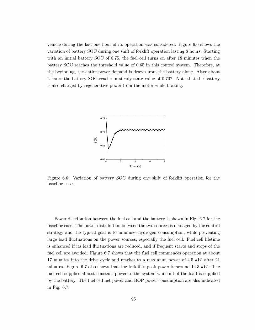
vehicle during the last one hour of its operation was considered. Figure 6.6 shows thevariation of battery SOC during one shift of forklift operation lasting 8 hours. Startingwith an initial battery SOC of 0.75, the fuel cell turns on after 18 minutes when thebattery SOC reaches the threshold value of 0.65 in this control system. Therefore, atthe beginning, the entire power demand is drawn from the battery alone. After about2 hours the battery SOC reaches a steady-state value of 0.707. Note that the batteryis also charged by regenerative power from the motor while braking.

0 2 4 6 80.60

0.65

0.70

0.75

SOC

Time (h)

Figure 6.6: Variation of battery SOC during one shift of forklift operation for thebaseline case.

Power distribution between the fuel cell and the battery is shown in Fig. 6.7 for thebaseline case. The power distribution between the two sources is managed by the controlstrategy and the typical goal is to minimize hydrogen consumption, while preventinglarge load fluctuations on the power sources, especially the fuel cell. Fuel cell lifetimeis enhanced if its load fluctuations are reduced, and if frequent starts and stops of thefuel cell are avoided. Figure 6.7 shows that the fuel cell commences operation at about17 minutes into the drive cycle and reaches to a maximum power of 4.5 kW after 21minutes. Figure 6.7 also shows that the forklift’s peak power is around 14.3 kW . Thefuel cell supplies almost constant power to the system while all of the load is suppliedby the battery. The fuel cell net power and BOP power consumption are also indicatedin Fig. 6.7.

95

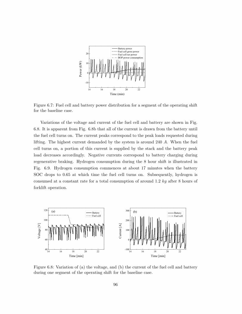
14 16 18 20 22

-10

0

10

20

Pow

er (k

W)

Time (min)

Battery power Fuel cell gross power Fuel cell net power BOP power consumption

Figure 6.7: Fuel cell and battery power distribution for a segment of the operating shiftfor the baseline case.

Variations of the voltage and current of the fuel cell and battery are shown in Fig.6.8. It is apparent from Fig. 6.8b that all of the current is drawn from the battery untilthe fuel cell turns on. The current peaks correspond to the peak loads requested duringlifting. The highest current demanded by the system is around 240 A. When the fuelcell turns on, a portion of this current is supplied by the stack and the battery peakload decreases accordingly. Negative currents correspond to battery charging duringregenerative braking. Hydrogen consumption during the 8 hour shift is illustrated inFig. 6.9. Hydrogen consumption commences at about 17 minutes when the batterySOC drops to 0.65 at which time the fuel cell turns on. Subsequently, hydrogen isconsumed at a constant rate for a total consumption of around 1.2 kg after 8 hours offorklift operation.

14 16 18 20 2240

60

80

100

120 (a)

Vol

tage

[V]

Time [min]

Battery Fuel cell

14 16 18 20 22-100

0

100

200

300 (b)

Cur

rent

[A]

Time [min]

Battery Fuel cell

Figure 6.8: Variation of (a) the voltage, and (b) the current of the fuel cell and batteryduring one segment of the operating shift for the baseline case.

96

0 2 4 6 8

0.0

0.4

0.8

1.2

1.6

Hyd

roge

n co

nsum

ptio

n [k

g]

Time [h]

Figure 6.9: Hydrogen consumption during one operating shift and for the baseline case.

6.4.2 Effect of battery size on hydrogen consumption

The size of the lead acid battery implemented in the system was varied to determine thehybrid combination that not only meets the system requirements, but also minimizeshydrogen consumption and downsizes the fuel cell stack. Batteries with different capac-ities have different weights and internal resistances which makes it difficult to predictthe optimal size for a specific purpose. The optimal size is also highly dependent onthe application and control strategy. Batteries with 80, 110 and 135 Ah were combinedwith a 110 cell PEMFC stack in this study. The battery weights are 170.1, 230, and284.2 kg, respectively. Another case studied consisted of two strings of 55 Ah batteries(119 kg each) in parallel combined with the same 110 cell stack. The forklift operatedfor 8 hours with an initial battery SOC of 0.75 and simulations were conducted for bothdrive cycles with the first control strategy. In order to accurately compare the hydrogenconsumption between the different cases, it is necessary to ensure that the final batterySOC is the same for all cases. A simple calculation was carried out to extrapolate thehydrogen consumption for a final SOC of 0.7. The results are summarized in Table 6.2.

Table 6.2: Effect of battery size on hydrogen consumption.Battery capacity Final SOC Hydrogen consumption (kg)

(Ah) Drive cycle 1 Drive cycle 2 Drive cycle 1 Drive cycle 280 0.709/0.7 0.718 / 0.7 1.233 / 1.179 0.991/0.883110 0.708 / 0.7 0.718 / 0.7 1.187 / 1.113 0.988/0.839135 0.708 / 0.7 0.718 / 0.7 1.191 / 1.110 0.988/0.8052×55 0.717 / 0.7 0.724 / 0.7 1.085 / 0.945 0.927/0.729

97

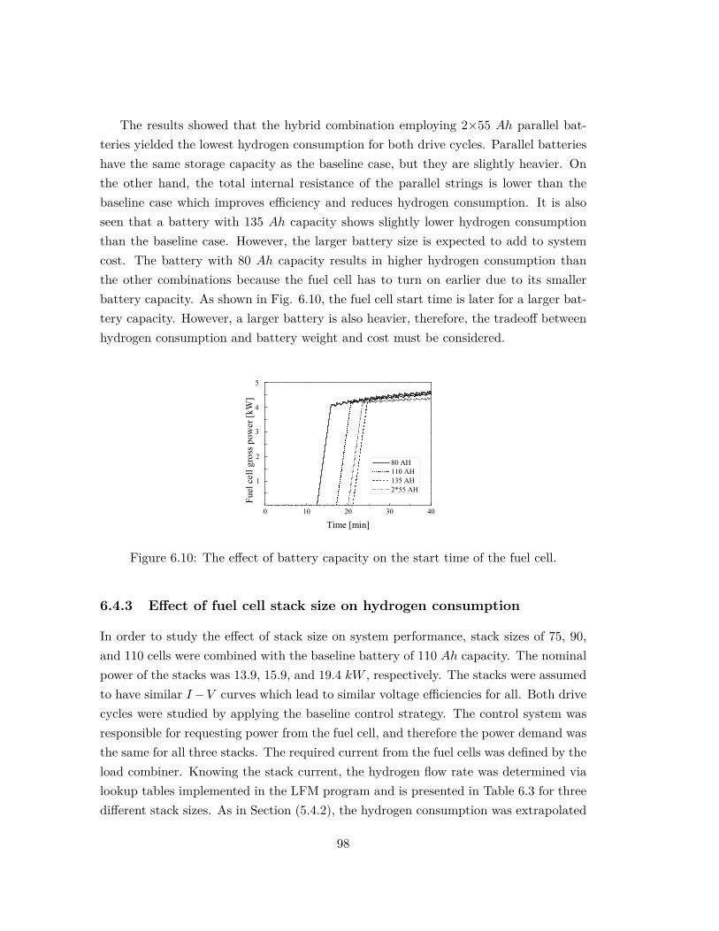
The results showed that the hybrid combination employing 2×55 Ah parallel bat-teries yielded the lowest hydrogen consumption for both drive cycles. Parallel batterieshave the same storage capacity as the baseline case, but they are slightly heavier. Onthe other hand, the total internal resistance of the parallel strings is lower than thebaseline case which improves efficiency and reduces hydrogen consumption. It is alsoseen that a battery with 135 Ah capacity shows slightly lower hydrogen consumptionthan the baseline case. However, the larger battery size is expected to add to systemcost. The battery with 80 Ah capacity results in higher hydrogen consumption thanthe other combinations because the fuel cell has to turn on earlier due to its smallerbattery capacity. As shown in Fig. 6.10, the fuel cell start time is later for a larger bat-tery capacity. However, a larger battery is also heavier, therefore, the tradeoff betweenhydrogen consumption and battery weight and cost must be considered.

0 10 20 30 40

5

4

3

2

1

Fuel

cel

l gro

ss p

ower

[kW

]

Time [min]

80 AH 110 AH 135 AH 2*55 AH

Figure 6.10: The effect of battery capacity on the start time of the fuel cell.

6.4.3 Effect of fuel cell stack size on hydrogen consumption

In order to study the effect of stack size on system performance, stack sizes of 75, 90,and 110 cells were combined with the baseline battery of 110 Ah capacity. The nominalpower of the stacks was 13.9, 15.9, and 19.4 kW , respectively. The stacks were assumedto have similar I−V curves which lead to similar voltage efficiencies for all. Both drivecycles were studied by applying the baseline control strategy. The control system wasresponsible for requesting power from the fuel cell, and therefore the power demand wasthe same for all three stacks. The required current from the fuel cells was defined by theload combiner. Knowing the stack current, the hydrogen flow rate was determined vialookup tables implemented in the LFM program and is presented in Table 6.3 for threedifferent stack sizes. As in Section (5.4.2), the hydrogen consumption was extrapolated

98

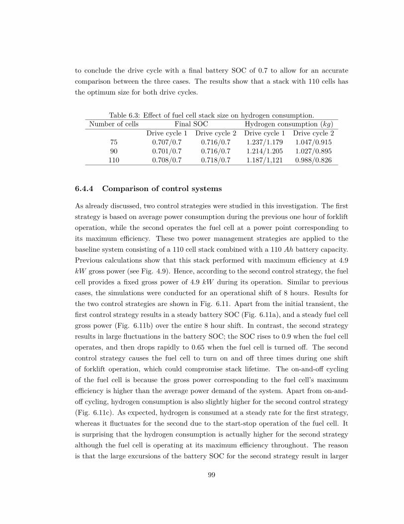
to conclude the drive cycle with a final battery SOC of 0.7 to allow for an accuratecomparison between the three cases. The results show that a stack with 110 cells hasthe optimum size for both drive cycles.

Table 6.3: Effect of fuel cell stack size on hydrogen consumption.Number of cells Final SOC Hydrogen consumption (kg)

Drive cycle 1 Drive cycle 2 Drive cycle 1 Drive cycle 275 0.707/0.7 0.716/0.7 1.237/1.179 1.047/0.91590 0.701/0.7 0.716/0.7 1.214/1.205 1.027/0.895110 0.708/0.7 0.718/0.7 1.187/1,121 0.988/0.826

6.4.4 Comparison of control systems

As already discussed, two control strategies were studied in this investigation. The firststrategy is based on average power consumption during the previous one hour of forkliftoperation, while the second operates the fuel cell at a power point corresponding toits maximum efficiency. These two power management strategies are applied to thebaseline system consisting of a 110 cell stack combined with a 110 Ah battery capacity.Previous calculations show that this stack performed with maximum efficiency at 4.9kW gross power (see Fig. 4.9). Hence, according to the second control strategy, the fuelcell provides a fixed gross power of 4.9 kW during its operation. Similar to previouscases, the simulations were conducted for an operational shift of 8 hours. Results forthe two control strategies are shown in Fig. 6.11. Apart from the initial transient, thefirst control strategy results in a steady battery SOC (Fig. 6.11a), and a steady fuel cellgross power (Fig. 6.11b) over the entire 8 hour shift. In contrast, the second strategyresults in large fluctuations in the battery SOC; the SOC rises to 0.9 when the fuel celloperates, and then drops rapidly to 0.65 when the fuel cell is turned off. The secondcontrol strategy causes the fuel cell to turn on and off three times during one shiftof forklift operation, which could compromise stack lifetime. The on-and-off cyclingof the fuel cell is because the gross power corresponding to the fuel cell’s maximumefficiency is higher than the average power demand of the system. Apart from on-and-off cycling, hydrogen consumption is also slightly higher for the second control strategy(Fig. 6.11c). As expected, hydrogen is consumed at a steady rate for the first strategy,whereas it fluctuates for the second due to the start-stop operation of the fuel cell. Itis surprising that the hydrogen consumption is actually higher for the second strategyalthough the fuel cell is operating at its maximum efficiency throughout. The reasonis that the large excursions of the battery SOC for the second strategy result in larger

99

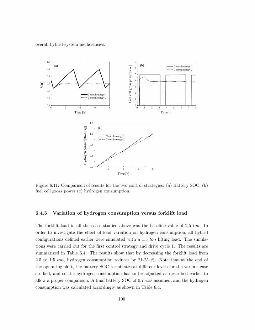
overall hybrid-system inefficiencies.

0 2 4 6 80.4

0.5

0.6

0.7

0.8

0.9

1.0(a)

SOC

Time [h]

Control strategy 1 Control strategy 2

0 1 2 3 4 5 6 7 80

1

2

3

4

5

6

7(b)

Fuel

cel

l gro

ss p

ower

[kW

]

Time [h]

Control strategy 1 Control strategy 2

2 4 6 80.0

0.4

0.8

1.2

1.6

(C)

Hyd

roge

n co

nsum

ptio

n [k

g]

Time [h]

Control strategy 1 Control strategy 2

Figure 6.11: Comparison of results for the two control strategies: (a) Battery SOC; (b)fuel cell gross power (c) hydrogen consumption.

6.4.5 Variation of hydrogen consumption versus forklift load

The forklift load in all the cases studied above was the baseline value of 2.5 ton. Inorder to investigate the effect of load variation on hydrogen consumption, all hybridconfigurations defined earlier were simulated with a 1.5 ton lifting load. The simula-tions were carried out for the first control strategy and drive cycle 1. The results aresummarized in Table 6.4. The results show that by decreasing the forklift load from2.5 to 1.5 ton, hydrogen consumption reduces by 21-25 %. Note that at the end ofthe operating shift, the battery SOC terminates at different levels for the various casestudied, and so the hydrogen consumption has to be adjusted as described earlier toallow a proper comparison. A final battery SOC of 0.7 was assumed, and the hydrogenconsumption was calculated accordingly as shown in Table 6.4.

100

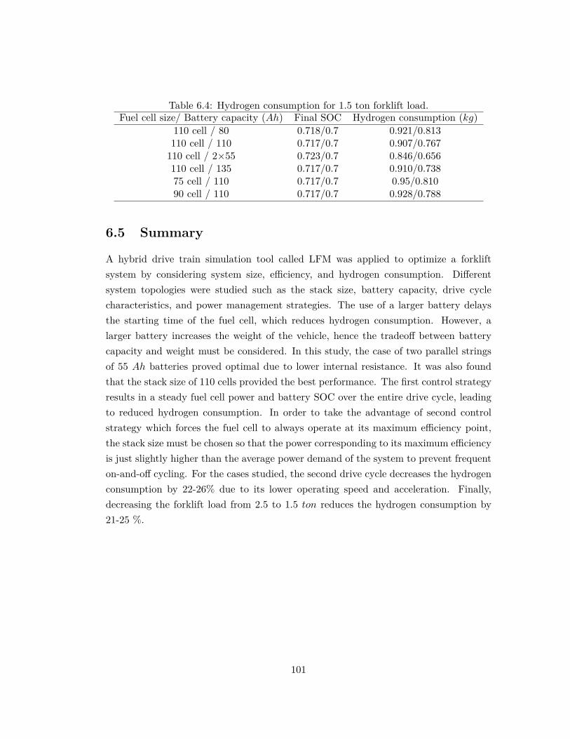
Table 6.4: Hydrogen consumption for 1.5 ton forklift load.Fuel cell size/ Battery capacity (Ah) Final SOC Hydrogen consumption (kg)

110 cell / 80 0.718/0.7 0.921/0.813110 cell / 110 0.717/0.7 0.907/0.767110 cell / 2×55 0.723/0.7 0.846/0.656110 cell / 135 0.717/0.7 0.910/0.73875 cell / 110 0.717/0.7 0.95/0.81090 cell / 110 0.717/0.7 0.928/0.788

6.5 Summary

A hybrid drive train simulation tool called LFM was applied to optimize a forkliftsystem by considering system size, efficiency, and hydrogen consumption. Differentsystem topologies were studied such as the stack size, battery capacity, drive cyclecharacteristics, and power management strategies. The use of a larger battery delaysthe starting time of the fuel cell, which reduces hydrogen consumption. However, alarger battery increases the weight of the vehicle, hence the tradeoff between batterycapacity and weight must be considered. In this study, the case of two parallel stringsof 55 Ah batteries proved optimal due to lower internal resistance. It was also foundthat the stack size of 110 cells provided the best performance. The first control strategyresults in a steady fuel cell power and battery SOC over the entire drive cycle, leadingto reduced hydrogen consumption. In order to take the advantage of second controlstrategy which forces the fuel cell to always operate at its maximum efficiency point,the stack size must be chosen so that the power corresponding to its maximum efficiencyis just slightly higher than the average power demand of the system to prevent frequenton-and-off cycling. For the cases studied, the second drive cycle decreases the hydrogenconsumption by 22-26% due to its lower operating speed and acceleration. Finally,decreasing the forklift load from 2.5 to 1.5 ton reduces the hydrogen consumption by21-25 %.

101

Chapter 7

Conclusion remarks

The main goal of this research was to study different fuel cell systems and find out thesystem with the highest electrical efficiency and less complexity for application in a 10kW forklift truck. This would be achieved by:

1. Modelling and optimization of the fuel cell system followed by some experimentaltests.

2. Investigation about anode recirculation.

3. Implementing of the fuel cell system in a virtual forklift.

7.1 Summary of findings

• Step 1: Modeling and optimization of the fuel cell and BOP

The overall system comprises of a PEM fuel cell, a compressor, an air humidifier, aset of heat exchangers and liquid pumps. As already discussed many components weredeveloped over years and already exist in DNA library. The only components whichwere needed to be modeled for investigation of the PEMFC system were humidifier andfuel cell stack. The developed model of each components are steady state and zerodimensional. For modeling the humidifier only mass balance has been considered andthe inlet and outlet temperature of the humidifier were defined by experimental set upwith the same operating conditions as the model. In other words it is acting like amixer in which dry air enters and depends on inlet temperature of the stack, requiredamount of water is added to it in order to reach to the desired level of humidity. Thepreliminary PEMFC model was based on the polynomial equations which have been

102

drived from the experimental data available from experimental setup of Ballard PEMfuel cell stack. Such equations can be mentioned as current–voltage relation, air andfuel pressure drop through the stack, etc. This stack model was then implementedin a fuel cell system with different layouts. Four system setup configurations werepresented. These were listed as single stack without recirculation (case A), single stackwith recirculation (case B), serial stack without recirculation (case C) and serial stackwith recirculation (case D). The calculations have been carried out for two sets of cellnumbers which are equal to 75 and 110 cells. For 75 number of cells the efficiency inthe basic case (case A) is 34% which is quite low. Various approaches for efficiencyimprovement have been studied to reach system efficiencies of about 50%. The resultsshowed that anode recirculation loop increases the efficiency in both single and serialstack design, but its effect is much larger in the single stack compared serial stackdesign. For 110 number of cells and Uf= 0.8 efficiency improvement due to anoderecirculation is about 10% for single stack compared to about 2% in serial stack design.Another issue which is discussed in this study is about cell arrangement. It is foundthat without recirculation loop, serial stack design has a higher efficiency comparedsingle stack, around 7% higher. However, for the systems with anode recirculation,(case B and case D) the efficiency of the single stack design is about 1% higher thanthe serial stack layout. Therefore single stack with recirculation (case B) is proposedas the most efficient fuel cell system because of its high efficiency and simplicity. Afterthermodynamic analysis of the proposed system configuration the most efficient fuelcell system (case B) has been chosen for development and optimization. To furtherdevelop the current fuel cell system model with more level of details the experimentalstack model was replaced by a a zero dimensional, steady state PEMFC model basedon theoretical and semi-empirical equations. The model takes into account the effectsof pressure losses, water crossovers, humidity aspects and voltage over-potentials inthe cells. The modeling approaches are based on the electrochemical reactions takingplace in a PEMFC. The models have been validated against the experimental data fromstack manual, provided by stack manufacturer. The polarization curve shows a verygood agreement with the experimental data. Afterward the behavior of PEMFC incooperation with BOP in a system was presented in terms of power production as wellas efficiency. Moreover a parametric study revealed the sensitivity of the system todifferent operating conditions to give an increased understanding of the stack and BOP.In addition recommendations have been given for water and thermal management of thesystem by investigation different coolants as well as operating conditions. The resultsshowed that proper humidification of the system as well as operating temperature of

103

the stack have a high influence on average cell voltage. By variation of humidity of theinlet air from 95 to 25%, the voltage may drop by 29%. However polarization curvedoes not change while decreasing the inlet humidity from 95 to 70%. By increasingthe stack temperature to 80

C for all the currents studied here and keeping the inlettemperatures unchanged, system efficiency decreases by 8% compared to the baselinecase. The higher the temperature, the higher the mass flow is needed for humidificationand water production cannot meet this requirement. This effect can be partly improvedby reducing the temperature gradient as the operating temperature increases.

In the cooling system by substituting liquid water with water-ethylene glycol mix-ture of 50%, the mass flow of coolant increases with about 32-33% in the inner loopand 60-65% in the outer loop for all range of current. However, the system efficiencydrops from 0.1 at very low current to 1.17% at the highest current studied here. Thevariation of mass flow and efficiency is more significant when the gas coolants, R134Aand R404A, are used in the system. Therefore, it is not reasonable to use gases coolantsin the system because they consume most of the electrical power and thereby systemefficiencies decreases considerably. Finally comparing the coolant mass flows at differenttemperatures show that by increasing coolant temperature from 30 to 45

C, the massflow increases by 68-80%. Meaning that to have more compact heat exchangers, thenlower temperature for the coolant is advantageous.

• Step 2: Development of ejector design

In the second step of this project, CFD technique has been used to design and analyzean ejector for anode recirculation of PEMFC system applied in a forklift truck. Since theejector is integrated in the PEMFC system, its operating conditions should be adjustedaccording to the fuel cell load fluctuations to cover the current variation of the stack from0-180 A. In order for the ejector to operate in the largest possible range of load, differentapproaches (with fixed nozzle and variable nozzle ejectors) have been investigated. Forthe first approach an ejector has been designed so that it could operate at the maximumload and mass flow rate. Then different geometries have been investigated in order tooptimize the ejector. The optimization is carried out not only by considering the bestperformance of ejector at maximum load with operation in the larger range as priority,but also catching the design point at maximum load even though it does not have thebest efficiency at such point. The geometry analysis showed that diameter ratios (ς) isthe key parameter in designing the ejector, and by choosing ς = 3.9 at Dt = 0.74 theejector can operate from 85-180A properly. However, in order to increase the operatingrange, another ejector was designed for maximum current of 85A. By optimization the

104

second ejector it was found that it could operate 100% at 85A and down to 90% at 60A.The third approach was applying an ejector with variable nozzle diameter. The resultsshowed that such ejector can also operate 100% at 180A down to 90% at 60A. However,in practice it is more difficult to manufacture an ejector with variable nozzle comparedto an ejector with the fixed nozzle diameter, but it could be the best choice for havingthe greatest entrainment ratio in the system.

• Step 3: Implementating of the fuel cell system in a virtual forklift

To continue this project, a hybrid drive train simulation tool called LFM was appliedto optimize a forklift system by considering system size, efficiency, and hydrogen con-sumption. LFM is a component based program which operates in Matlab/Simulink.The program consists of different subsystems which are linked using electrical, mechan-ical, and control signals and construct a virtual vehicle. The calculations are based onthe vehicle drive cycle. In other words, the drive cycle is implemented in the programas an input. At each time step, LFM simulator calculates and compares the currentvehicle speed with the given speed and tries to minimize their difference. In this pro-gram different system topologies were studied such as the stack size (75, 90 and 110cells), battery capacity (80, 110, 135, 2×55 AH), drive cycle characteristics, and powermanagement strategies. The baseline control strategy was to maintain the battery SOCat the desired level such that the fuel cell starts to supply power when the batterySOC drops to the minimum threshold of 0.65. However, the second control strategyemphasizes the efficiency of the fuel cell. For the second control system, the fuel cellturns on when SOC(t) reaches the threshold value of 65% and supplies a constant powercorresponding to its maximum efficiency. The fuel cell then switches off when SOC(t)reaches 90% so that the battery may take the advantage of regenerative power.

The results showed that the use of a larger battery delays the starting time of thefuel cell, which reduces hydrogen consumption. However, a larger battery increases theweight of the vehicle, hence the trade off between battery capacity and weight mustbe considered. In this study, the case of two parallel strings of 55 Ah batteries provedoptimal due to lower internal resistance. It was also found that the stack size of 110cells provided the best performance. The first control strategy results in a steady fuelcell power and battery SOC over the entire drive cycle, leading to reduced hydrogenconsumption. In order to take the advantage of second control strategy which forcesthe fuel cell to always operate at its maximum efficiency point, the stack size must bechosen so that the power corresponding to its maximum efficiency is just slightly higherthan the average power demand of the system to prevent frequent on-and-off cycling.

105

For the cases studied, the second drive cycle decreases the hydrogen consumption by22-26% due to its lower operating speed and acceleration. Finally, decreasing the forkliftload from 2.5 to 1.5 ton reduces the hydrogen consumption by 21-25 %.

7.2 Recommendation for further work

7.2.1 Humidifier component model

As it has been elaborated in the study, proper humidification of the air and the fuelstreams contributes strongly to optimal fuel cell performance. In the present study asimple component for humidifier has been modeled which only takes into account themass transfer between the species (water and air), however in practice the heat transferbetween the two phases as well as water condensation/evaporation should be considered.Therefore having a comprehensive model of humidifier is strongly recommended.

7.2.2 Improvement the present PEMFC model

In this study a general zero-dimensional model of PEMFC was developed. The modelwas based on theoretical and semi-empirical equations. A well-known model was used tocapture the experimental polarization curve which was published by the stack manufac-turer. The available experimental data are only within the range of operating conditionswhich are recommended by the stack manufacturer and there is no data available out ofthat range. Even though the applied model was already validated by other researchersagainst a lot of experimental data, yet it could be a good idea to gain experimentalpolarization curve for different ranges of pressure or operating temperature. On theother hand having some measurement regarding the amount of liquid water at the an-ode and cathode outlet separately and validation with the theoretical results could beadvantageous.

The concentration overpotential results from concentration gradient of the reactantsand products between the flow channel and the catalyst reaction site. The concentrationloss increases as the current increases, until at certain current the transport of speciesis not fast enough to feed the electrochemical reaction. This current is called limitingcurrent and can be found out through experimental tests. Since concentration loss isdominant at very high currents which is not the case here and since steady state behaviorof the system is discussed in this study, this term does not play a significant role andwas neglected in the calculations. However it is important in dynamic simulation andpart load applications. By finding this parameter through experimental set up, the

106

concentration overpotential can be properly modeled.Having a zero-dimensional model imposes many simplification into the model. In

order to have a more realistic model with enhanced level of details, development of aCFD model of PEMFC could be very interesting. Moreover having a dynamic modelinstead of steady state could give more insight of a real system considering start up andload changes and etc.

7.2.3 Improvement of the present ejector design

The current ejector design is a steady state 2-D model based on axisymmetric solution inwhich the species transport model for the mixture flow of hydrogen and water vapor hasbeen activated. To improve the present design a transient 3-D model can replace a 2-Dmodel by considering multiphase flow model instead of species transport model. Anotherissue which can be taken into consideration is manufacturing an ejector and testingdifferent parameters to validate the numerical output. Moreover as it was presented inthe results, an ejector with variable nozzle could be much more effective than a fixednozzle ejector. Manufacturing a variable nozzle ejector with a proper control systemmight need much effort, but it could be a valuable step in future development of thepresent fuel cell system.

7.2.4 Virtual forklift

As already discussed a hybrid drive train simulation tool called LFM was applied tooptimize a forklift system by considering system size, efficiency, and hydrogen con-sumption. The input to the program is the drive cycle of the forklift and the rest of thecalculations are carried out in respect to that. In the calculations the drive cycle andacceleration was assumed with regard to the maximum vehicle and fork speed limit. Inorder to take the advantage of simulation results one should provide the real data fordrive cycle and compare the results of the simulation tool with experimental data.

At the present study the performance of a forklift truck powered by a fuel cell/batteryhybrid system has been discussed. The fuel cell is connected in parallel to the battery,such that the fuel cell experiences a relatively constant load while all the traction loadsare directly powered by the battery. While a battery alone significantly reduces theload variations of the fuel cell, an ultracapacitor reduces them even further. There-fore adding an ultracapacitor to the forklift system can lead to the even better resultsspecially from life time perspective.

107

Bibliography

[1] Mark9 SSL of Ballard Company, Product manual and integration guide, 2008.

[2] R. K. Ahluwalia and X. Wang, “Direct hydrogen fuel cell systems for hybrid vehi-cles,” Journal of Power Sources, vol. 139, pp. 152–164, 2005.

[3] Y. Wang, K. S. Chen, J. Mishler, and X. C. Adroher, “A review of polymer elec-trolyte membrane fuel cells: Technology, applications, and needs on fundamentalresearch,” Applied Energy, vol. 88, pp. 981–1007, 2011.

[4] B. D. James, J. A. Kalinoski, and K. N. Baum, Directed technologies I. Massproduction cost estimation for direct H2 PEM fuel cell systems for automotiveapplications. 2008 update 2009, p. 10.

[5] L. Martins, J. Gardolinski, J. Vargas, J. Ordonez, S. Amico, and M. Forte, “Theexperimental validation of a simplified pemfc simulation model for design and op-timization purposes,” Applied Thermal Engineering, vol. 29, pp. 3036–3048, 2009.

[6] M. Cordner, M. M. G. Offer, T. Hanten, E. Spofforth-Jones, S. Tippetts,A. Agrawal, L. Bannar-Martin, L. Harito, A. Johnson, R. Clague, F. Marquis,A. Heyes, Y. Hardalupas, and N. Brandon, “Designing, building, testing and rac-ing a low-cost fuel cell range extender for a motorsport application,” Journal ofPower Sources, vol. 195, pp. 7838–7848, 2010.

[7] R. M. Rao and R. Rengaswamy, “Optimization study of an agglomerate model forplatinum reduction and performance in pem fuel cell cathode,” Chemical Engineer-ing Research and Design, vol. 84, pp. 952–964, 2006.

[8] S.-D. Yim, W.-Y. Lee, Y.-G. Yoon, Y.-J. Sohn, G.-G. Park, T.-H. Yang, and C.-S.Kim, “Optimization of bifunctional electrocatalyst for pem unitized regenerativefuel cell,” Electrochimica Acta, vol. 50, pp. 713–718, 2004.

108

[9] J. Wu, X. Z. Yuan, J. J. Martin, HaijiangWang, J. Zhang, J. Shen, S. Wu, andW. Merida, “A review of pem fuel cell durability: Degradation mechanisms andmitigation strategies,” Journal of Power Sources, vol. 184, pp. 104–119, 2008.

[10] S. E. Iyuke, A. B. Mohamad, A. A. H. Kadhum, W. R. Daud, and C. Rachid,“Improved membrane and electrode assemblies for proton exchange membrane fuelcells,” Journal of Power Sources, vol. 114, pp. 195–202, 2003.

[11] S. M. C. Ang, D. J. Brett, and E. S. Fraga, “A multi-objective optimisation modelfor a general polymer electrolyte membrane fuel cell system,” Journal of PowerSources, vol. 195, pp. 2754–2763, 2010.

[12] H.-W. Wu and H.-W. Ku, “The optimal parameters estimation for rectangu-lar cylinders installed transversely in the flow channel of pemfc from a three-dimensional pemfc model and the taguchi method,” Applied Energy, vol. 88,pp. 4879–4890, 2011.

[13] V. Meidanshahi and G. Karimi, “Dynamic modeling, optimization and control ofpower density in a pem fuel cell,” Applied Energy, vol. 93, pp. 98–105, 2012.

[14] W.-M. Yan, X.-D. Wang, D.-J. Lee, X.-X. Zhang, Y.-F. Guo, and A. Su, “Experi-mental study of commercial size proton exchange membrane fuel cell performance,”Applied Energy, vol. 88, pp. 392–396, 2011.

[15] Y. Tang, W. Yuan, M. Pan, Z. Li, G. Chen, and Y. Li, “Experimental investigationof dynamic performance and transient responses of a kw-class pem fuel cell stackunder various load changes,” Applied Energy, vol. 87, pp. 1410–1417, 2010.

[16] J. Nolan and J. Kolodziej, “Modeling of an automotive fuel cell thermal system,”Journal of Power Sources, vol. 195, pp. 4743–4752, 2010.

[17] R. Anderson, M. Blanco, X. Bi, and D. P. Wilkinson, “Anode water removal andcathode gas diffusion layer flooding in a proton exchange membrane fuel cell,”International Journal of Hydrogen Energy, vol. 37, pp. 16093–16103, 2012.

[18] T. V. Nguyen and M. W. Knobbe, “A liquid water management strategy for pemfuel cell stacks,” Journal of Power Sources, vol. 114, pp. 70–79, 2003.

[19] D. Picot, R. Metkemeijer, J. Bezian, and L. Rouveyre, “Impact of the water sym-metry factor on humidification and cooling strategies for pem fuel cell stacks,”Journal of Power Sources, vol. 75, pp. 251–260, 1998.

109

[20] K. Jiao and X. Li, “Water transport in polymer electrolyte membrane fuel cells,”Progress in Energy and Combustion Science, vol. 37, pp. 221–291, 2011.

[21] D. Gerteisen, T. Heilmann, and C. Ziegler, “Modeling the phenomena of dehydra-tion and flooding of a polymer electrolyte membrane fuel cell,” Journal of PowerSources, vol. 187, pp. 165–181, 2009.

[22] F. N. Buchi and S. Srinivasa, “Operating proton exchange membrane fuel cellswithout external humidification of the reactant gases,” Electrochem. Soc, vol. 144,pp. 2767–2772, 1997.

[23] A. Shah, G.-S. Kimb, W. Gervais, A. Young, K. Promislow, J. Li, and S. Ye, “Theeffects of water and microstructure on the performance of polymer electrolyte fuelcells,” Journal of Power Sources, vol. 160, pp. 1251–1268, 2006.

[24] J.-H. Wee, “Applications of proton exchange membrane fuel cell systems,” Renew-able and Sustainable Energy Reviews, vol. 11, pp. 1720–1738, 2007.

[25] J. Stumper and C. Stone, “Recent advances in fuel cell technology at ballard,”Journal of Power Sources, vol. 176, pp. 468–476, 2008.

[26] T. Keränen, H. Karimäki, J. Viitakangas, J. Vallet, J. Ihonen, P. Hyötylä,H. Uusalo, and T. Tingelöf, “Development of integrated fuel cell hybrid powersource for electric forklift,” Journal of Power Sources, vol. 196, pp. 9058–9068,2011.

[27] A. Elgowainy, L. Gaines, and M. Wang, “Fuel-cycle analysis of early market appli-cations of fuel cells: Forklift propulsion systems and distributed power generation,”International Journal of Hydrogen Energy, vol. 34, pp. 3557–3570, 2009.

[28] B. Elmegaard, Simulation of boiler dynamics - Development, Evaluation and Ap-plication of a General Energy System Simulation Tool. PhD thesis, Technical Uni-versity of Denmark, 1999.

[29] C. Spiegel, Designing and building fuel cells. Mc Graw Hill, 2007.

[30] J. Laminie and A. Dicks, Fuel Cell Systems Explained. John Wiley & Sons Ltd,2000.

[31] P. K. Das, X. Li, and Z.-S. Liu, “Analysis of liquid water transport in cathodecatalyst layer of pem fuel cells,” International Journal of Hydrogen Energy, vol. 35,pp. 2403–2416, 2010.

110

[32] www.h2logic.com.

[33] J. Yuan, M. Rokni, and B. SundeŽn, “A numerical investigation of gas flow andheat transfer in proton exchange membrane fuel cells,” Numerical Heat Transfer,Part A, vol. 44, pp. 255–280, 2003.

[34] M. Santarelli, M. Torchio, and P. Cochis, “Parameters estimation of a pem fuelcell polarization curve and analysis of their behavior with temperature,” Journalof Power Sources, vol. 159, pp. 824–835, 2006.

[35] G. Prentice, Electrochemical engineering principles. Prentice Hall International,1991.

[36] V. A. Danilov and M. O. Tade, “An alternative way of estimating anodic and ca-thodic transfer coefficients from pemfc polarization curves,” Chemical EngineeringJournal, vol. 156, pp. 496–499, 2010.

[37] C. Berger, Handbook of fuel cell technology. Prentice-Hall, 1968.

[38] J. C. Amphlett, R. M. Baumert, R. F. Mann, B. A. Peppley, P. R. Roberge,and T. J. Harris, “Performance modeling of the ballard mark iv solid polymer elec-trolyte fuel cell : Ii . empirical model development,” Journal of The ElectrochemicalSociety, vol. 142, pp. 9–15, 1995.

[39] R. F. Mann, J. C. Amphlett, M. A. Hooper, H. M. Jensen, B. A. Peppley, and P. R.Roberge, “Development and application of a generalised steady-state electrochem-ical model for a pem fuel cell,” Journal of Power Sources, vol. 86, pp. 173–180,2000.

[40] D. Candusso, F. Harel, A. D. Bernardinis, X. François, M. Péra, D. Hissel,P. Schott, G. Coquery, and J.-M. Kauffmann, “Characterisation and modelling ofa 5kw pemfc for transportation applications,” International Journal of HydrogenEnergy, vol. 31, pp. 1019–1030, 2006.

[41] K. Mammar and A. Chaker, “Modelling and fuzzy logic control of pem fuel cellsystem power generation for residential application,” Journal of Electrical & Elec-tronics Engineering, vol. 9, pp. 1073–1081, 2009.

[42] A. Cisar, “in: Proceedings of 26th intersociety energy conversion conference, iecec,”1991.

111

[43] M. Santarelli and M. Torchio, “Experimental analysis of the effects of the operatingvariables on the performance of a single pemfc,” Energy Conversion and Manage-ment, vol. 48, pp. 40–51, 2007.

[44] L. Zhang, M. Pan, and S. Quan, “Model predictive control of water managementin pemfc,” Journal of Power Sources, vol. 180, pp. 322–329, 2008.

[45] T. E. Springer, T. A. Zawodzinski, and S. Gottesfeld, “Polymer electrolyte fuel cellmodel,” Journal of Electrochemical Society, vol. 138, pp. 2334–2341, 1991.

[46] P. Spinelli, C. Francia, E. Ambrosio, and M. Lucariello, “Semi-empirical evaluationof pemfc electro-catalytic activity,” Journal of Power Sources, vol. 178, pp. 517–524, 2008.

[47] S. Haji, “Analytical modeling of pem fuel cell i-v curve,” Renewable Energy, vol. 36,pp. 451–458, 2011.

[48] A. W. Al-Dabbagh, L. Lu, and A. Mazza, “Modelling, simulation and control of aproton exchange membrane fuel cell (pemfc) power system,” International Journalof Hydrogen Energy, vol. 35, pp. 5061–5069, 2010.

[49] P. Pei, WuYang, and P. Li, “Numerical prediction on an automotive fuel cell drivingsystem,” International Journal of Hydrogen Energy, vol. 31, pp. 361–369, 2006.

[50] L. Martins, J. Gardolinski, J. Vargas, J. Ordonez, S. Amico, and M. Forte, “Theexperimental validation of a simplified pemfc simulation model for design and op-timization purposes,” Applied Thermal Engineering, vol. 29, pp. 3036–3048, 2009.

[51] V. Gurau, F. Barbir, and H. Liu, “An analytical solution of a half-cell model forpem fuel cells,” Journal of The Electrochemical Society, vol. 147, pp. 2468–2477,2000.

[52] T. Murahashi, M. Naiki, and E. Nishiyama, “Water transport in the protonexchange-membrane fuel cell: Comparison of model computation and measure-ments of effective drag,” Journal of Power Sources, vol. 162, pp. 1130–1136, 2006.

[53] S. Shimpalee and S. Dutta, “Numerical prediction of temperature distribution inpem fuel cells,” Numerical Heat Transfer, Part A, vol. 38, pp. 111–128, 2000.

[54] G. Zhang and S. G. Kandlikar, “A critical review of cooling techniques in protonexchange membrane fuel cell stacks,” International Journal of Hydrogen Energy,vol. 37, pp. 2412–2429, 2012.

112

[55] S. G. Kandlikar and Z. Lu, “Thermal management issues in a pemfc stack - a briefreview of current status,” Applied Thermal Engineering, vol. 29, pp. 1276–1280,2009.

[56] “Numerical investigation of liquid water cooling for a proton exchange membranefuel cell stack,” Journal of Heat Transfer Engineering, vol. 32, pp. 151–167, 2011.

[57] A. Faghri and Z. Guo, “Challenges and opportunities of thermal management issuesrelated to fuel cell technology and modeling,” International Journal of Heat andMass Transfer, vol. 48, pp. 3891–3920, 2005.

[58] G. Frank, “Prospects and requirements of high temperature pemfc,” in Proceedingsof the 2nd European PEFC Forum, Lucerne, Switzerland, 2003.

[59] J. Zhang, Z. Xie, J. Zhang, Y. Tang, C. Song, T. Navessin, Z. Shi, D. Song,H. Wang, D. P. Wilkinson, Z.-S. Liu, and S. Holdcroft, “High temperature pemfuel cells,” Journal of Power Sources, vol. 160, pp. 872–891, 2006.

[60] H. Li, Y. Tang, Z. Wang, Z. Shi, S. Wu, D. Song, J. Zhang, K. Fatih, J. Zhang,H. Wang, Z. Liu, R. Abouatallah, and A. Mazza, “A review of water flooding issuesin the proton exchange membrane fuel cell,” Journal of Power Sources, vol. 178,pp. 103–117, 2008.

[61] Y. Shao, G. Yin, Z. Wang, and Y. Gao, “Proton exchange membrane fuel cellfrom low temperature to high temperature: Material challenges,” Journal of PowerSources, vol. 167, pp. 235–242, 2007.

[62] S. J. Andreasen, J. R. Vang, and S. K. Kær, “High temperature pem fuel cellperformance characterisation with co and co2 using electrochemical impedancespectroscopy,” International Journal of Hydrogen Energy, vol. 36, pp. 9815–9830,2011.

[63] F. N. Buchi and S. Srinivasan, “Operating proton exchange membrane fuel cellswithout external humidification of the reactant gases,” Journal of ElectrochemSociety, vol. 144, pp. 2767–2772, 1997.

[64] S. Tsushima and S. Hirai, “In situ diagnostics for water transport in proton ex-change membrane fuel cells,” Progress in Energy and Combustion Science, vol. 37,pp. 204–220, 2011.

113

[65] J.-W. Ahn and S.-Y. Choe, “Coolant controls of a pem fuel cell system,” Journalof Power Sources, vol. 179, pp. 252–264, 2008.

[66] J. He, S.-Y. Choe, and C.-O. Hong, “Analysis and control of a hybrid fuel deliverysystem for a polymer electrolyte membrane fuel cell,” Journal of Power Sources,vol. 185, pp. 973–984, 2008.

[67] J. He, J. Ahn, and S.-Y. Choe, “Analysis and control of a fuel delivery systemconsidering a two-phase anode model of the polymer electrolyte membrane fuel cellstack,” Journal of Power Sources, vol. 196, pp. 4655–4670, 2011.

[68] D. A. Brunner, S. Marcks, M. Bajpai, A. K. Prasad, and S. G. Advani, “Design andcharacterization of an electronically controlled variable flow rate ejector for fuel cellapplications,” International Journal of Hydrogen Energy, vol. 37, pp. 4457–4466,2012.

[69] M. Kim, Y.-J. Sohn, C.-W. Cho, W.-Y. Lee, and C.-S. Kim, “Customized designfor the ejector to recirculate a humidified hydrogen fuel in a submarine pemfc,”Journal of Power Sources, vol. 176, pp. 529–533, 2008.

[70] D.-W. Sun, “Comparative study of the performance of an ejector refrigeration cycleoperating with various refrigerants,” Energy Conversion & Management, vol. 40,pp. 873–884, 1999.

[71] D.-W. Sun, “Experimental investigation of the performance characteristics of asteam jet refrigeration system,” Energy Sources, vol. 19, pp. 349–367, 1997.

[72] M. Colarossi, N. Trask, D. P. Schmidt, and M. J. Bergander, “Multidimensionalmodeling of condensing two-phase ejector flow,” International Journal of Refriger-ation, vol. 35, pp. 290–299, 2012.

[73] Y. Jia and C. Wenjian, “Area ratio effects to the performance of air-cooled ejectorrefrigeration cycle with r134a refrigerant,” Energy Conversion and Management,vol. 53, pp. 240–246, 2012.

[74] G. Grazzini, A. Milazzo, and D. Paganini, “Design of an ejector cycle refrigerationsystem,” Energy Conversion and Management, vol. 54, pp. 38–46, 2012.

[75] F. Marsano, L. Magistri, and A. Massardo, “Ejector performance influence ona solid oxide fuel cell anodic recirculation system,” Journal of Power Sources,vol. 129, pp. 216–228, 2004.

114

[76] J. Milewski, A. Miller, and J. Salacinski, “Off-design analysis of sofc hybrid sys-tem,” International Journal of Hydrogen Energy, vol. 32, pp. 687–698, 2007.

[77] Y. Zhu, Y. Li, and W. Cai, “Control oriented modeling of ejector in anode gasrecirculation solid oxygen fuel cell systems,” Energy Conversion and Management,vol. 52, pp. 1181–1189, 2011.

[78] Y. Zhu and Y. Li, “New theoretical model for convergent nozzle ejector in theproton exchange membrane fuel cell system,” Journal of Power Sources, vol. 191,pp. 510–519, 2009.

[79] B. Huang, J. Chang, C. Wang, and V. Petrenko, “A 1-d analysis of ejector perfor-mance,” International Journal of Refrigeration, vol. 22, pp. 354–364, 1999.

[80] J. G. del Valle, J. M. S. iz Jabardo, F. C. Ruiz, and J. S. J. Alonso, “A one dimen-sional model for the determination of an ejector entrainment ratio,” InternationalJournal of Refrigeration, vol. 35, pp. 772–784, 2012.

[81] M. Rokni and B. Sunden, “On developments of k-tau and k-omega models fornear-wall turbulence of engineering duct flows,” International Journal of TransportPhenomena, vol. 11, pp. 233–253, 2009.

[82] F. Mentor, “Two-equation eddy-viscosity turbulence models for engineering appli-cations,” AIAA Journal, vol. 32, pp. 1598–1605, 1994.

[83] Y. Zhu, W. Cai, and C. W. andYanzhong Li, “Fuel ejector design and simulationmodel for anodic recirculation sofc system,” Journal of Power Sources, vol. 173,pp. 437–449, 2007.

[84] G. E. Alves, Ejector design and performance, ch. 5, pp. 69–79. University ofDelaware, 1951.

[85] E. Hosseinzadeh and M. Rokni, “Development and validation of a simple analyticalmodel of the proton exchange membrane fuel cell (pemfc) in a fork-lift truck powersystem,” International Journal of Green Energy, 2012, In press.

[86] Y. Zhu, W. Cai, C. Wen, and Y. Li, “Numerical investigation of geometry parame-ters for design of high performance ejectors,” Applied Thermal Engineering, vol. 29,pp. 898–905, 2009.

115

[87] M. Nakagawa, A. Marasigan, T. Matsukawa, and A. Kurashina, “Experimentalinvestigation on the effect of mixing length on the performance of two-phase ejectorfor co2 refrigeration cycle with and without heat exchanger,” International Journalof Refrigeration, vol. 34, pp. 1604–1613, 2011.

[88] P. Bubna, D. Brunner, S. G. Advani, and A. K. Prasad, “Prediction-based optimalpower management in a fuel cell/battery plug-in hybrid vehicle,” Journal of PowerSources, vol. 195, pp. 6699–6708, 2010.

[89] M. Ouyang, L. Xu, J. Li, L. Lu, D. Gao, and Q. Xie, “Performance comparisonof two fuel cell hybrid buses with different powertrain and energy managementstrategies,” Journal of Power Sources, vol. 163, pp. 467–479, 2006.

[90] A. Schell, H. Peng, D. Tran, E. Stamos, C.-C. Lin, and M. J. Kim, “Modellingand control strategy development for fuel cell electric vehicles,” Annual Reviews inControl, vol. 29, pp. 159–168, 2005.

[91] M. D. Francesco and E. Arato, “Start-up analysis for automotive pem fuel cellsystems,” Journal of Power Sources, vol. 108, pp. 41–52, 2002.

[92] J. Wang, Y. Chen, and Q. Chen, “A fuel cell city bus with three drivetrain config-uration,” Journal of Power Sources, vol. 159, pp. 1205–1213, 2006.

[93] D. Brown, M. Alexander, D. Brunner, S. G. Advani, and A. K. Prasad, “Drive-train simulator for a fuel cell hybrid vehicle,” Journal of Power Sources, vol. 183,pp. 275–281, 2008.

[94] P. Bubna, D. Brunner, J. J. G. Jr., S. G. Advani, and A. K. Prasad, “Analysis,operation and maintenance of a fuel cell/battery series-hybrid bus for urban transitapplications,” Journal of Power Sources, vol. 195, pp. 3939–3949, 2010.

116

Appendix A

DNA source code

A.1 Humidifier component model code

117

humidifier.for 1/6

C********************************************************************** SUBROUTINE HUMIDIFIER(KOMTY,ANTLK,ANTEX,ANTED,ANTKN,ANTPK,ANTM1, : ANTM2,ANTSW,DYCOM,MEDIE,ANTME,VARME,ANTEL, : VAREL,MDOT,P,H,E,Q,PAR,RES,X_J)C**********************************************************************CC HUMIDIFIER is a model of a humidifier. There is no heat transferC equation.C***********************************************************************CCA FKOMP − INPUT − Flag with the value:CA 1: Initialize the component.CA 2: Initialize with actual system.CA 3: Fluid composition calculation (constant).CA 4: Find residuals.CA 5: Find residuals and check variables.CA 6: Output information about component.CA MDOT − INPUT − Massflows from nodes.CA P − INPUT − Pressure in nodes.CA X_J − INPUT − Fluid composition.CA KOMTY − OUTPUT − Component name.CA ANTPK − OUTPUT − Number of parameters for the component.CA ANTLK − OUTPUT − Number of equations in the component.CA ANTEX − OUTPUT − Number of independent equations in the component.CA ANTED − OUTPUT − Number of differential independent equations.CA ANTKN − OUTPUT − Number of nodes connected to the component.CA ANTM1 − OUTPUT − Number of massflows in the first conservation ofCA mass equation.CA ANTM2 − OUTPUT − Number of massflows in the second.CA DYCOM − OUTPUT − Type of conservation equations (static or dynamicCA mass and internal energy on side 1 and 2 respectively;CA and dynamic solid internal energy).CA MEDIE − IN/OUT − Media (fluid) of the connected nodes.CA The values mean :CA CA −4 : Any gasCA ANTME − OUTPUT − Number of fluids with variable composition.CA VARME − OUTPUT − Pointer to fluid numbers (with variable composition).CA ANTEL − OUTPUT − Number of computed compounds in these variable fluids.CA VAREL − OUTPUT − Compound numbers in variable fluids.CA RES − OUTPUT − Residuals for the component.CCL XMIX Composition of the mixture.CL K_PAR Parameter description.CL K_LIG Equation description.

CL K_BET Condition description.CL K_MED Media description.CC Subroutines : COMINFC CCP Programmer : Elham Hosseinzadeh (ehos), TES, MEK, DTU, 2010

C***********************************************************************CC Including the common "environment"C INCLUDE ’ENVIRO.INI’ INCLUDE ’THERPROP.DEC’CC Parameter variablesC INTEGER ANTLK, ANTEX, ANTED, ANTKN, MEDIE(6), ANTPK, : ANTM1, ANTM2,ANTSW, ANTME, VARME(4), ANTEL(4), : VAREL(ANTST,4),NCELL DOUBLE PRECISION X_J(MAXME,ANTST), RES(15),MDOT(4),P(4), : H(4),PAR(2) CHARACTER*3 DYCOM(5) CHARACTER*80 KOMTYCC Local variablesC INTEGER K_MED(6)

humidifier.for 2/6

DOUBLE PRECISION NDOTCO2_IN, $ NDOTH2O_IN, NDOTO2_IN, NDOTN2_IN, NDOTAR_IN, NDOTN2_OUT, $ NDOTO2_OUT, NDOTCO2_OUT, $ NDOTH2O_OUT, NDOTAR_OUT, XCO2_IN, $ XH2O_IN, XO2_IN, XN2_IN, XAR_IN, $ XCO2_OUT, XH2O_OUT, XO2_OUT, XN2_OUT, XAR_OUT, $ M_AIR_IN, M_AIR_OUT, T3, T4,DP,

$ NDOTH2O_INW, NDOTO2_INW, NDOTN2_INW, NDOTAR_INW, NDOTN2_OUTW, $ NDOTO2_OUTW, NDOTCO2_OUTW, NDOTCO2_INW, $ NDOTH2O_OUTW, NDOTAR_OUTW, XCO2_INW, $ XH2O_INW, XO2_INW, XN2_INW, XAR_INW, $ XCO2_OUTW, XH2O_OUTW, XO2_OUTW, XN2_OUTW, XAR_OUTW, $ M_AIR_INW, M_AIR_OUTW,

$ S, X, DUM,V,T2,T1,E,Q, $ MV_IN, MA_IN, PSAT_WATER,PV_WATER,PA_OUT,RH,MV_OUT,MV3, $ HUMIDITY,MV_HUM,NV_HUM,PSAT_WATER_IN,W_IN,PA_IN,HUMIDITY_IN CHARACTER*100 K_PAR(1),K_STAT(1) CHARACTER*500 K_LIG(39), K_BET, KOMDSC,K_INP,K_GRAF CHARACTER*100 KMEDDS(6) EXTERNAL COMINF INCLUDE ’THERPROP.INI’

C======================================================================= GOTO (100,200,300,400,400,200) FKOMP RETURN

C−−−−−−−−−−−−−−−−−−−−−−−−−−−−−−−−−−−−−−−−−−−−−−−−−−−−−−−−−−−−−−−−−−−−−−−C Component nameC−−−−−−−−−−−−−−−−−−−−−−−−−−−−−−−−−−−−−−−−−−−−−−−−−−−−−−−−−−−−−−−−−−−−−−− 100 CONTINUE KOMTY = ’HUMIDIFIER’

GOTO 9999C−−−−−−−−−−−−−−−−−−−−−−−−−−−−−−−−−−−−−−−−−−−−−−−−−−−−−−−−−−−−−−−−−−−−−−−C Component characteristicsC−−−−−−−−−−−−−−−−−−−−−−−−−−−−−−−−−−−−−−−−−−−−−−−−−−−−−−−−−−−−−−−−−−−−−−− 200 CONTINUE KOMTY = ’HUMIDIFIER’ ANTKN = 5 ANTPK = 2 ANTLK = 15 ANTM1 = 4 MEDIE(1) = ANYGAS$ MEDIE(2) = ANYGAS$ MEDIE(3) = ANYGAS$ MEDIE(4) = ANYGAS$ MEDIE(5) = HEAT$ ANTME = 4 VARME(1) = NODE1$ VARME(2) = NODE2$ VARME(3) = NODE3$ ANTEL(3) = 5 VAREL(1,3)=O2$ VAREL(2,3)=N2$ VAREL(3,3)=CO2$ VAREL(4,3)=H2O_G$ VAREL(5,3)=AR$ VARME(4) = NODE4$ ANTEL(4) = 5 VAREL(1,4)=O2$ VAREL(2,4)=N2$ VAREL(3,4)=CO2$ VAREL(4,4)=H2O_G$ VAREL(5,4)=AR$ IF (FKOMP.EQ.6) GOTO 600*** FKOMP = 3 GOTO 9999C−−−−−−−−−−−−−−−−−−−−−−−−−−−−−−−−−−−−−−−−−−−−−−−−−−−−−−−−−−−−−−−−−−−−−−−C Fluid composition calculation (constant).C−−−−−−−−−−−−−−−−−−−−−−−−−−−−−−−−−−−−−−−−−−−−−−−−−−−−−−−−−−−−−−−−−−−−−−−

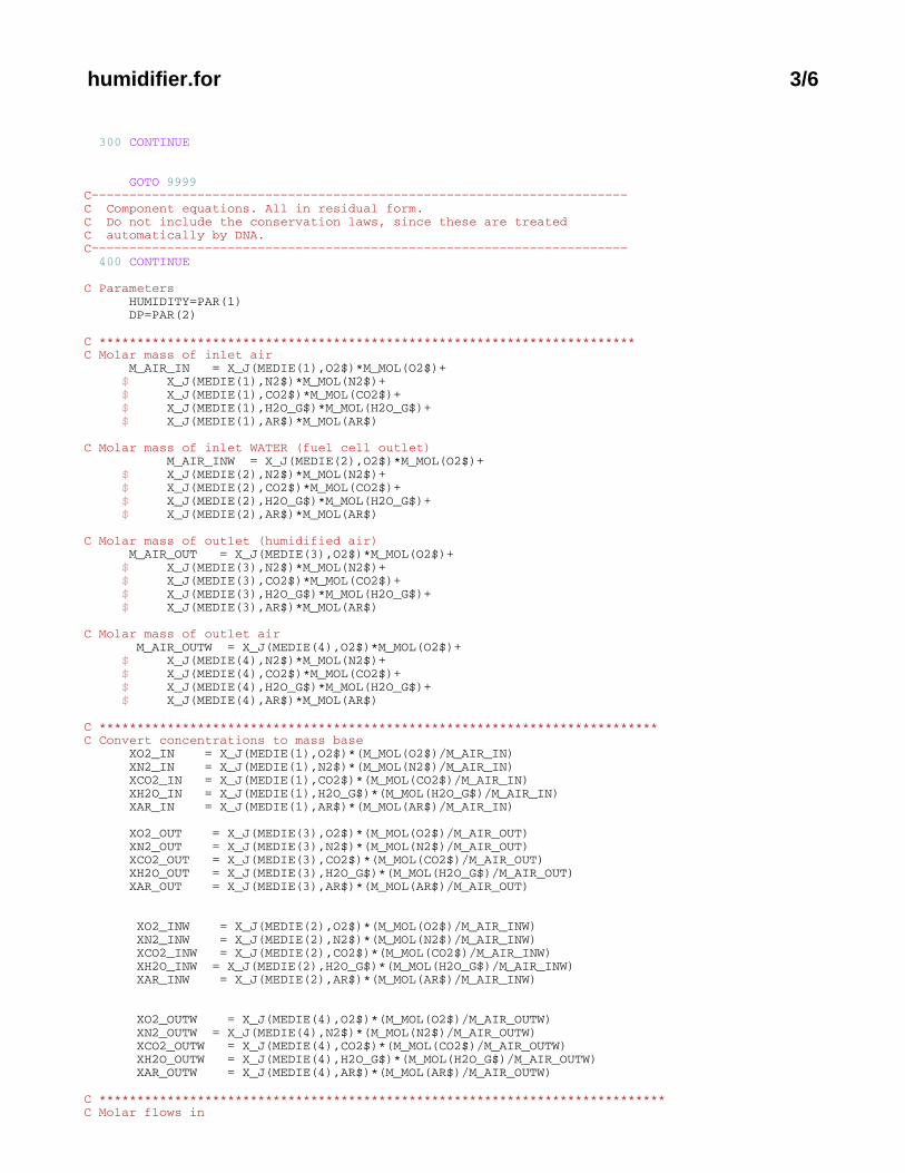
humidifier.for 3/6

300 CONTINUE

GOTO 9999C−−−−−−−−−−−−−−−−−−−−−−−−−−−−−−−−−−−−−−−−−−−−−−−−−−−−−−−−−−−−−−−−−−−−−−−C Component equations. All in residual form.C Do not include the conservation laws, since these are treatedC automatically by DNA.C−−−−−−−−−−−−−−−−−−−−−−−−−−−−−−−−−−−−−−−−−−−−−−−−−−−−−−−−−−−−−−−−−−−−−−− 400 CONTINUE

C Parameters HUMIDITY=PAR(1) DP=PAR(2) C ***********************************************************************C Molar mass of inlet air M_AIR_IN = X_J(MEDIE(1),O2$)*M_MOL(O2$)+ $ X_J(MEDIE(1),N2$)*M_MOL(N2$)+ $ X_J(MEDIE(1),CO2$)*M_MOL(CO2$)+ $ X_J(MEDIE(1),H2O_G$)*M_MOL(H2O_G$)+ $ X_J(MEDIE(1),AR$)*M_MOL(AR$)

C Molar mass of inlet WATER (fuel cell outlet) M_AIR_INW = X_J(MEDIE(2),O2$)*M_MOL(O2$)+ $ X_J(MEDIE(2),N2$)*M_MOL(N2$)+ $ X_J(MEDIE(2),CO2$)*M_MOL(CO2$)+ $ X_J(MEDIE(2),H2O_G$)*M_MOL(H2O_G$)+ $ X_J(MEDIE(2),AR$)*M_MOL(AR$)

C Molar mass of outlet (humidified air) M_AIR_OUT = X_J(MEDIE(3),O2$)*M_MOL(O2$)+ $ X_J(MEDIE(3),N2$)*M_MOL(N2$)+ $ X_J(MEDIE(3),CO2$)*M_MOL(CO2$)+ $ X_J(MEDIE(3),H2O_G$)*M_MOL(H2O_G$)+ $ X_J(MEDIE(3),AR$)*M_MOL(AR$)

C Molar mass of outlet air M_AIR_OUTW = X_J(MEDIE(4),O2$)*M_MOL(O2$)+ $ X_J(MEDIE(4),N2$)*M_MOL(N2$)+ $ X_J(MEDIE(4),CO2$)*M_MOL(CO2$)+ $ X_J(MEDIE(4),H2O_G$)*M_MOL(H2O_G$)+ $ X_J(MEDIE(4),AR$)*M_MOL(AR$)

C **************************************************************************C Convert concentrations to mass base XO2_IN = X_J(MEDIE(1),O2$)*(M_MOL(O2$)/M_AIR_IN) XN2_IN = X_J(MEDIE(1),N2$)*(M_MOL(N2$)/M_AIR_IN) XCO2_IN = X_J(MEDIE(1),CO2$)*(M_MOL(CO2$)/M_AIR_IN) XH2O_IN = X_J(MEDIE(1),H2O_G$)*(M_MOL(H2O_G$)/M_AIR_IN) XAR_IN = X_J(MEDIE(1),AR$)*(M_MOL(AR$)/M_AIR_IN) XO2_OUT = X_J(MEDIE(3),O2$)*(M_MOL(O2$)/M_AIR_OUT) XN2_OUT = X_J(MEDIE(3),N2$)*(M_MOL(N2$)/M_AIR_OUT) XCO2_OUT = X_J(MEDIE(3),CO2$)*(M_MOL(CO2$)/M_AIR_OUT) XH2O_OUT = X_J(MEDIE(3),H2O_G$)*(M_MOL(H2O_G$)/M_AIR_OUT) XAR_OUT = X_J(MEDIE(3),AR$)*(M_MOL(AR$)/M_AIR_OUT)

XO2_INW = X_J(MEDIE(2),O2$)*(M_MOL(O2$)/M_AIR_INW) XN2_INW = X_J(MEDIE(2),N2$)*(M_MOL(N2$)/M_AIR_INW) XCO2_INW = X_J(MEDIE(2),CO2$)*(M_MOL(CO2$)/M_AIR_INW) XH2O_INW = X_J(MEDIE(2),H2O_G$)*(M_MOL(H2O_G$)/M_AIR_INW) XAR_INW = X_J(MEDIE(2),AR$)*(M_MOL(AR$)/M_AIR_INW)

XO2_OUTW = X_J(MEDIE(4),O2$)*(M_MOL(O2$)/M_AIR_OUTW) XN2_OUTW = X_J(MEDIE(4),N2$)*(M_MOL(N2$)/M_AIR_OUTW) XCO2_OUTW = X_J(MEDIE(4),CO2$)*(M_MOL(CO2$)/M_AIR_OUTW) XH2O_OUTW = X_J(MEDIE(4),H2O_G$)*(M_MOL(H2O_G$)/M_AIR_OUTW) XAR_OUTW = X_J(MEDIE(4),AR$)*(M_MOL(AR$)/M_AIR_OUTW)

C ***************************************************************************C Molar flows in

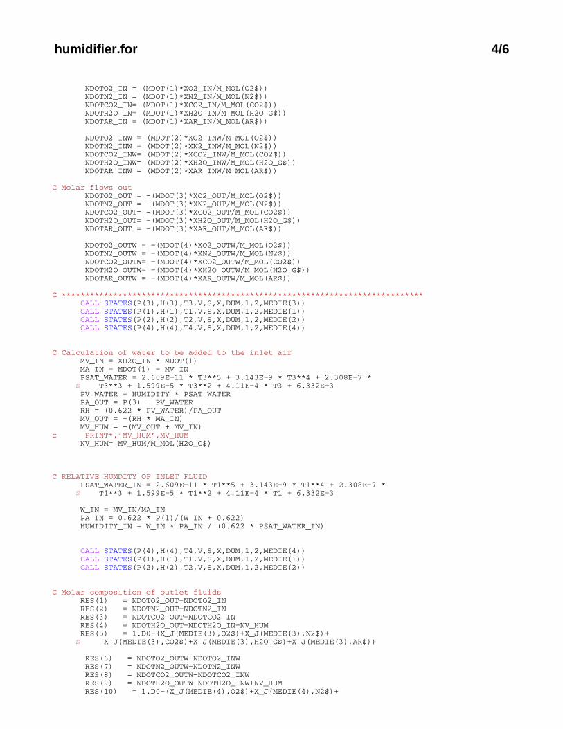
humidifier.for 4/6

NDOTO2_IN = (MDOT(1)*XO2_IN/M_MOL(O2$)) NDOTN2_IN = (MDOT(1)*XN2_IN/M_MOL(N2$)) NDOTCO2_IN= (MDOT(1)*XCO2_IN/M_MOL(CO2$)) NDOTH2O_IN= (MDOT(1)*XH2O_IN/M_MOL(H2O_G$)) NDOTAR_IN = (MDOT(1)*XAR_IN/M_MOL(AR$))

NDOTO2_INW = (MDOT(2)*XO2_INW/M_MOL(O2$)) NDOTN2_INW = (MDOT(2)*XN2_INW/M_MOL(N2$)) NDOTCO2_INW= (MDOT(2)*XCO2_INW/M_MOL(CO2$)) NDOTH2O_INW= (MDOT(2)*XH2O_INW/M_MOL(H2O_G$)) NDOTAR_INW = (MDOT(2)*XAR_INW/M_MOL(AR$)) C Molar flows out NDOTO2_OUT = −(MDOT(3)*XO2_OUT/M_MOL(O2$)) NDOTN2_OUT = −(MDOT(3)*XN2_OUT/M_MOL(N2$)) NDOTCO2_OUT= −(MDOT(3)*XCO2_OUT/M_MOL(CO2$)) NDOTH2O_OUT= −(MDOT(3)*XH2O_OUT/M_MOL(H2O_G$)) NDOTAR_OUT = −(MDOT(3)*XAR_OUT/M_MOL(AR$))

NDOTO2_OUTW = −(MDOT(4)*XO2_OUTW/M_MOL(O2$)) NDOTN2_OUTW = −(MDOT(4)*XN2_OUTW/M_MOL(N2$)) NDOTCO2_OUTW= −(MDOT(4)*XCO2_OUTW/M_MOL(CO2$)) NDOTH2O_OUTW= −(MDOT(4)*XH2O_OUTW/M_MOL(H2O_G$)) NDOTAR_OUTW = −(MDOT(4)*XAR_OUTW/M_MOL(AR$))

C ***************************************************************************** CALL STATES(P(3),H(3),T3,V,S,X,DUM,1,2,MEDIE(3)) CALL STATES(P(1),H(1),T1,V,S,X,DUM,1,2,MEDIE(1)) CALL STATES(P(2),H(2),T2,V,S,X,DUM,1,2,MEDIE(2)) CALL STATES(P(4),H(4),T4,V,S,X,DUM,1,2,MEDIE(4))

C Calculation of water to be added to the inlet air MV_IN = XH2O_IN * MDOT(1) MA_IN = MDOT(1) − MV_IN PSAT_WATER = 2.609E−11 * T3**5 + 3.143E−9 * T3**4 + 2.308E−7 * $ T3**3 + 1.599E−5 * T3**2 + 4.11E−4 * T3 + 6.332E−3 PV_WATER = HUMIDITY * PSAT_WATER PA_OUT = P(3) − PV_WATER RH = (0.622 * PV_WATER)/PA_OUT MV_OUT = −(RH * MA_IN) MV_HUM = −(MV_OUT + MV_IN)c PRINT*,’MV_HUM’,MV_HUM NV_HUM= MV_HUM/M_MOL(H2O_G$)

C RELATIVE HUMDITY OF INLET FLUID PSAT_WATER_IN = 2.609E−11 * T1**5 + 3.143E−9 * T1**4 + 2.308E−7 * $ T1**3 + 1.599E−5 * T1**2 + 4.11E−4 * T1 + 6.332E−3

W_IN = MV_IN/MA_IN PA_IN = 0.622 * P(1)/(W_IN + 0.622) HUMIDITY_IN = W_IN * PA_IN / (0.622 * PSAT_WATER_IN)

CALL STATES(P(4),H(4),T4,V,S,X,DUM,1,2,MEDIE(4)) CALL STATES(P(1),H(1),T1,V,S,X,DUM,1,2,MEDIE(1)) CALL STATES(P(2),H(2),T2,V,S,X,DUM,1,2,MEDIE(2))

C Molar composition of outlet fluids RES(1) = NDOTO2_OUT−NDOTO2_IN RES(2) = NDOTN2_OUT−NDOTN2_IN RES(3) = NDOTCO2_OUT−NDOTCO2_IN RES(4) = NDOTH2O_OUT−NDOTH2O_IN−NV_HUM RES(5) = 1.D0−(X_J(MEDIE(3),O2$)+X_J(MEDIE(3),N2$)+ $ X_J(MEDIE(3),CO2$)+X_J(MEDIE(3),H2O_G$)+X_J(MEDIE(3),AR$))

RES(6) = NDOTO2_OUTW−NDOTO2_INW RES(7) = NDOTN2_OUTW−NDOTN2_INW RES(8) = NDOTCO2_OUTW−NDOTCO2_INW RES(9) = NDOTH2O_OUTW−NDOTH2O_INW+NV_HUM RES(10) = 1.D0−(X_J(MEDIE(4),O2$)+X_J(MEDIE(4),N2$)+

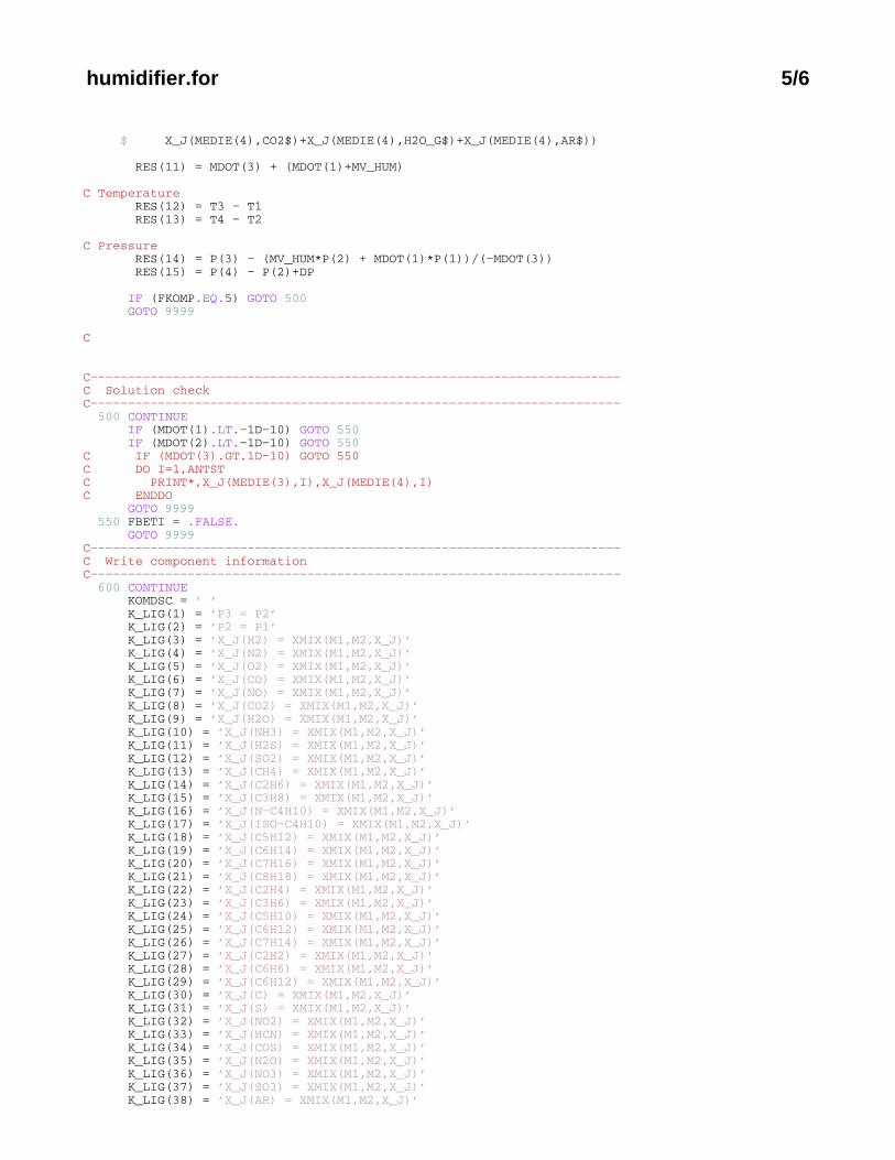
humidifier.for 5/6

$ X_J(MEDIE(4),CO2$)+X_J(MEDIE(4),H2O_G$)+X_J(MEDIE(4),AR$))

RES(11) = MDOT(3) + (MDOT(1)+MV_HUM)

C Temperature RES(12) = T3 − T1 RES(13) = T4 − T2

C Pressure RES(14) = P(3) − (MV_HUM*P(2) + MDOT(1)*P(1))/(−MDOT(3)) RES(15) = P(4) − P(2)+DP IF (FKOMP.EQ.5) GOTO 500 GOTO 9999

C

C−−−−−−−−−−−−−−−−−−−−−−−−−−−−−−−−−−−−−−−−−−−−−−−−−−−−−−−−−−−−−−−−−−−−−−−C Solution checkC−−−−−−−−−−−−−−−−−−−−−−−−−−−−−−−−−−−−−−−−−−−−−−−−−−−−−−−−−−−−−−−−−−−−−−− 500 CONTINUE IF (MDOT(1).LT.−1D−10) GOTO 550 IF (MDOT(2).LT.−1D−10) GOTO 550C IF (MDOT(3).GT.1D−10) GOTO 550C DO I=1,ANTSTC PRINT*,X_J(MEDIE(3),I),X_J(MEDIE(4),I)C ENDDO GOTO 9999 550 FBETI = .FALSE. GOTO 9999C−−−−−−−−−−−−−−−−−−−−−−−−−−−−−−−−−−−−−−−−−−−−−−−−−−−−−−−−−−−−−−−−−−−−−−−C Write component informationC−−−−−−−−−−−−−−−−−−−−−−−−−−−−−−−−−−−−−−−−−−−−−−−−−−−−−−−−−−−−−−−−−−−−−−− 600 CONTINUE KOMDSC = ’ ’ K_LIG(1) = ’P3 = P2’ K_LIG(2) = ’P2 = P1’ K_LIG(3) = ’X_J(H2) = XMIX(M1,M2,X_J)’ K_LIG(4) = ’X_J(N2) = XMIX(M1,M2,X_J)’ K_LIG(5) = ’X_J(O2) = XMIX(M1,M2,X_J)’ K_LIG(6) = ’X_J(CO) = XMIX(M1,M2,X_J)’ K_LIG(7) = ’X_J(NO) = XMIX(M1,M2,X_J)’ K_LIG(8) = ’X_J(CO2) = XMIX(M1,M2,X_J)’ K_LIG(9) = ’X_J(H2O) = XMIX(M1,M2,X_J)’ K_LIG(10) = ’X_J(NH3) = XMIX(M1,M2,X_J)’ K_LIG(11) = ’X_J(H2S) = XMIX(M1,M2,X_J)’ K_LIG(12) = ’X_J(SO2) = XMIX(M1,M2,X_J)’ K_LIG(13) = ’X_J(CH4) = XMIX(M1,M2,X_J)’ K_LIG(14) = ’X_J(C2H6) = XMIX(M1,M2,X_J)’ K_LIG(15) = ’X_J(C3H8) = XMIX(M1,M2,X_J)’ K_LIG(16) = ’X_J(N−C4H10) = XMIX(M1,M2,X_J)’ K_LIG(17) = ’X_J(ISO−C4H10) = XMIX(M1,M2,X_J)’ K_LIG(18) = ’X_J(C5H12) = XMIX(M1,M2,X_J)’ K_LIG(19) = ’X_J(C6H14) = XMIX(M1,M2,X_J)’ K_LIG(20) = ’X_J(C7H16) = XMIX(M1,M2,X_J)’ K_LIG(21) = ’X_J(C8H18) = XMIX(M1,M2,X_J)’ K_LIG(22) = ’X_J(C2H4) = XMIX(M1,M2,X_J)’ K_LIG(23) = ’X_J(C3H6) = XMIX(M1,M2,X_J)’ K_LIG(24) = ’X_J(C5H10) = XMIX(M1,M2,X_J)’ K_LIG(25) = ’X_J(C6H12) = XMIX(M1,M2,X_J)’ K_LIG(26) = ’X_J(C7H14) = XMIX(M1,M2,X_J)’ K_LIG(27) = ’X_J(C2H2) = XMIX(M1,M2,X_J)’ K_LIG(28) = ’X_J(C6H6) = XMIX(M1,M2,X_J)’ K_LIG(29) = ’X_J(C6H12) = XMIX(M1,M2,X_J)’ K_LIG(30) = ’X_J(C) = XMIX(M1,M2,X_J)’ K_LIG(31) = ’X_J(S) = XMIX(M1,M2,X_J)’ K_LIG(32) = ’X_J(NO2) = XMIX(M1,M2,X_J)’ K_LIG(33) = ’X_J(HCN) = XMIX(M1,M2,X_J)’ K_LIG(34) = ’X_J(COS) = XMIX(M1,M2,X_J)’ K_LIG(35) = ’X_J(N2O) = XMIX(M1,M2,X_J)’ K_LIG(36) = ’X_J(NO3) = XMIX(M1,M2,X_J)’ K_LIG(37) = ’X_J(SO3) = XMIX(M1,M2,X_J)’ K_LIG(38) = ’X_J(AR) = XMIX(M1,M2,X_J)’

humidifier.for 6/6

K_LIG(39) = ’X_J(SiO2) = XMIX(M1,M2,X_J)’ K_BET = ’MDOT1 \\gt 0 $ MDOT2 \\gt 0 $ MDOT3 \\lt 0’ K_PAR(1) = ’ ’ K_MED(1) = MEDIE(1) K_MED(2) = MEDIE(2) K_MED(3) = MEDIE(3) KMEDDS(1) = ’ ’ KMEDDS(2) = ’ ’ KMEDDS(3) = ’ ’ KMEDDS(4) = ’ ’ KMEDDS(5) = ’ ’ KMEDDS(6) = ’ ’

CALL COMINF(KOMTY,KOMDSC,1,1,1,1, $ K_MED,K_PAR,K_LIG,K_BET,KMEDDS,K_STAT,K_INP,K_GRAF) GOTO 9999C 9999 CONTINUE RETURN END

C=======================================================================C=======================================================================

A.2 Flow sheet of humidifier component model with nodenumbers

124

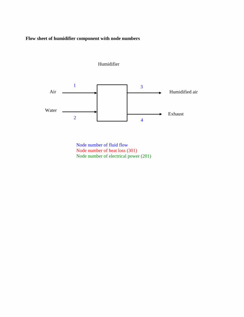
Humidifier

Air Humidified air

Water Exhaust

1

2

4

Flow sheet of humidifier component with node numbers

3

Node number of fluid flow Node number of heat loss (301) Node number of electrical power (201)

A.3 The source code of PEMFC component model basedon experimental correlations

126

pemfc3.for 1/5

C********************************************************************** SUBROUTINE PEMFC_EH3(KOMTY,ANTLK,ANTEX,ANTED,ANTKN,ANTPK,ANTM1, : ANTM2,ANTSW,DYCOM,MEDIE,ANTME,VARME,ANTEL, : VAREL,MDOT,P,H,E,Q,PAR,RES,X_J)C**********************************************************************CC PEMFC_EH3 is a model of a PEM Fuel Cell. The equations are extraxtedC from experimental data.

C***********************************************************************CCA FKOMP − INPUT − Flag with the value:CA 1: Initialize the component.CA 2: Initialize with actual system.CA 3: Fluid composition calculation (constant).CA 4: Find residuals.CA 5: Find residuals and check variables.CA 6: Output information about component.CA MDOT − INPUT − Massflows from nodes.CA P − INPUT − Pressure in nodes.CA X_J − INPUT − Fluid composition.CA KOMTY − OUTPUT − Component name.CA ANTPK − OUTPUT − Number of parameters for the component.CA ANTLK − OUTPUT − Number of equations in the component.CA ANTEX − OUTPUT − Number of independent equations in the component.CA ANTED − OUTPUT − Number of differential independent equations.CA ANTKN − OUTPUT − Number of nodes connected to the component.CA ANTM1 − OUTPUT − Number of massflows in the first conservation ofCA mass equation.CA ANTM2 − OUTPUT − Number of massflows in the second.CA DYCOM − OUTPUT − Type of conservation equations (static or dynamicCA mass and internal energy on side 1 and 2 respectively;CA and dynamic solid internal energy).CA MEDIE − IN/OUT − Media (fluid) of the connected nodes.CA The values mean :CA CA −4 : Any gasCA ANTME − OUTPUT − Number of fluids with variable composition.CA VARME − OUTPUT − Pointer to fluid numbers (with variable composition).CA ANTEL − OUTPUT − Number of computed compounds in these variable fluids.CA VAREL − OUTPUT − Compound numbers in variable fluids.CA RES − OUTPUT − Residuals for the component.CCL XMIX Composition of the mixture.CL K_PAR Parameter description.CL K_LIG Equation description.CL K_BET Condition description.CL K_MED Media description.CC Subroutines : COMINFC CCP Programmer : Elham Hosseinzadeh (ehos), TES, MEK, DTU, 2009

C***********************************************************************CC Including the common "environment"C INCLUDE ’ENVIRO.INI’ INCLUDE ’THERPROP.DEC’CC Parameter variablesC INTEGER ANTLK, ANTEX, ANTED, ANTKN, MEDIE(6), ANTPK, : ANTM1, ANTM2,ANTSW, ANTME, VARME(4), ANTEL(4), : VAREL(ANTST,4),NCELL DOUBLE PRECISION X_J(MAXME,ANTST), RES(13),MDOT(4),P(4), : H(4),E,Q(1),PAR(4) CHARACTER*3 DYCOM(5) CHARACTER*80 KOMTYCC Local variablesC INTEGER K_MED(6)

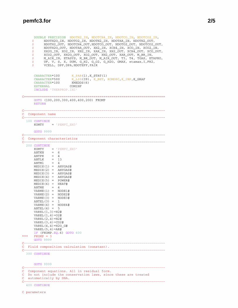
pemfc3.for 2/5

DOUBLE PRECISION NDOTH2_IN, NDOTCH4_IN, NDOTCO_IN, NDOTCO2_IN, $ NDOTH2O_IN, NDOTO2_IN, NDOTN2_IN, NDOTAR_IN, NDOTN2_OUT, $ NDOTH2_OUT, NDOTCH4_OUT,NDOTCO_OUT, NDOTO2_OUT, NDOTCO2_OUT, $ NDOTH2O_OUT, NDOTAR_OUT, XH2_IN, XCH4_IN, XCO_IN, XCO2_IN, $ XH2O_IN, XO2_IN, XN2_IN, XAR_IN, XH2_OUT, XCH4_OUT, XCO_OUT, $ XCO2_OUT, XH2O_OUT, XO2_OUT, XN2_OUT, XAR_OUT, M_BR_IN, $ M_AIR_IN, ETASYS, M_BR_OUT, M_AIR_OUT, T3, T4, TGAS, ETAPRO, $ UF, V, S, X, DUM, G_H2, G_O2, G_H2O, GMAX, etamax,I,FH2, $ VCELL, DPF,DPA,NDOTEFF,FAIR CHARACTER*100 K_PAR(1),K_STAT(1) CHARACTER*500 K_LIG(39), K_BET, KOMDSC,K_INP,K_GRAF CHARACTER*100 KMEDDS(6) EXTERNAL COMINF INCLUDE ’THERPROP.INI’

C======================================================================= GOTO (100,200,300,400,400,200) FKOMP RETURN

C−−−−−−−−−−−−−−−−−−−−−−−−−−−−−−−−−−−−−−−−−−−−−−−−−−−−−−−−−−−−−−−−−−−−−−−C Component nameC−−−−−−−−−−−−−−−−−−−−−−−−−−−−−−−−−−−−−−−−−−−−−−−−−−−−−−−−−−−−−−−−−−−−−−− 100 CONTINUE KOMTY = ’PEMFC_EH3’

GOTO 9999C−−−−−−−−−−−−−−−−−−−−−−−−−−−−−−−−−−−−−−−−−−−−−−−−−−−−−−−−−−−−−−−−−−−−−−−C Component characteristicsC−−−−−−−−−−−−−−−−−−−−−−−−−−−−−−−−−−−−−−−−−−−−−−−−−−−−−−−−−−−−−−−−−−−−−−− 200 CONTINUE KOMTY = ’PEMFC_EH3’ ANTKN = 6 ANTPK = 4 ANTLK = 13 ANTM1 = 4 MEDIE(1) = ANYGAS$ MEDIE(2) = ANYGAS$ MEDIE(3) = ANYGAS$ MEDIE(4) = ANYGAS$ MEDIE(5) = POWER$ MEDIE(6) = HEAT$ ANTME = 4 VARME(1) = NODE1$ VARME(2) = NODE2$ VARME(3) = NODE3$ ANTEL(3) = 1 VARME(4) = NODE4$ ANTEL(4) = 5 VAREL(1,3)=H2$ VAREL(1,4)=O2$ VAREL(2,4)=N2$ VAREL(3,4)=CO2$ VAREL(4,4)=H2O_G$ VAREL(5,4)=AR$ IF (FKOMP.EQ.6) GOTO 600*** FKOMP = 3 GOTO 9999C−−−−−−−−−−−−−−−−−−−−−−−−−−−−−−−−−−−−−−−−−−−−−−−−−−−−−−−−−−−−−−−−−−−−−−−C Fluid composition calculation (constant).C−−−−−−−−−−−−−−−−−−−−−−−−−−−−−−−−−−−−−−−−−−−−−−−−−−−−−−−−−−−−−−−−−−−−−−− 300 CONTINUE

GOTO 9999C−−−−−−−−−−−−−−−−−−−−−−−−−−−−−−−−−−−−−−−−−−−−−−−−−−−−−−−−−−−−−−−−−−−−−−−C Component equations. All in residual form.C Do not include the conservation laws, since these are treatedC automatically by DNA.C−−−−−−−−−−−−−−−−−−−−−−−−−−−−−−−−−−−−−−−−−−−−−−−−−−−−−−−−−−−−−−−−−−−−−−− 400 CONTINUE

C parameters

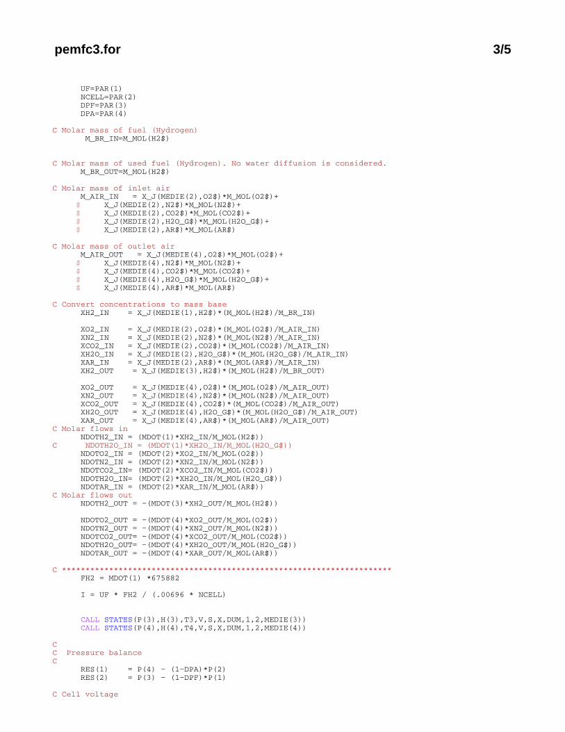
pemfc3.for 3/5

UF=PAR(1) NCELL=PAR(2) DPF=PAR(3) DPA=PAR(4) C Molar mass of fuel (Hydrogen) M_BR_IN=M_MOL(H2$)

C Molar mass of used fuel (Hydrogen). No water diffusion is considered. M_BR_OUT=M_MOL(H2$)

C Molar mass of inlet air M_AIR_IN = X_J(MEDIE(2),O2$)*M_MOL(O2$)+ $ X_J(MEDIE(2),N2$)*M_MOL(N2$)+ $ X_J(MEDIE(2),CO2$)*M_MOL(CO2$)+ $ X_J(MEDIE(2),H2O_G$)*M_MOL(H2O_G$)+ $ X_J(MEDIE(2),AR$)*M_MOL(AR$)

C Molar mass of outlet air M_AIR_OUT = X_J(MEDIE(4),O2$)*M_MOL(O2$)+ $ X_J(MEDIE(4),N2$)*M_MOL(N2$)+ $ X_J(MEDIE(4),CO2$)*M_MOL(CO2$)+ $ X_J(MEDIE(4),H2O_G$)*M_MOL(H2O_G$)+ $ X_J(MEDIE(4),AR$)*M_MOL(AR$)

C Convert concentrations to mass base XH2_IN = X_J(MEDIE(1),H2$)*(M_MOL(H2$)/M_BR_IN)

XO2_IN = X_J(MEDIE(2),O2$)*(M_MOL(O2$)/M_AIR_IN) XN2_IN = X_J(MEDIE(2),N2$)*(M_MOL(N2$)/M_AIR_IN) XCO2_IN = X_J(MEDIE(2),CO2$)*(M_MOL(CO2$)/M_AIR_IN) XH2O_IN = X_J(MEDIE(2),H2O_G$)*(M_MOL(H2O_G$)/M_AIR_IN) XAR_IN = X_J(MEDIE(2),AR$)*(M_MOL(AR$)/M_AIR_IN) XH2_OUT = X_J(MEDIE(3),H2$)*(M_MOL(H2$)/M_BR_OUT)

XO2_OUT = X_J(MEDIE(4),O2$)*(M_MOL(O2$)/M_AIR_OUT) XN2_OUT = X_J(MEDIE(4),N2$)*(M_MOL(N2$)/M_AIR_OUT) XCO2_OUT = X_J(MEDIE(4),CO2$)*(M_MOL(CO2$)/M_AIR_OUT) XH2O_OUT = X_J(MEDIE(4),H2O_G$)*(M_MOL(H2O_G$)/M_AIR_OUT) XAR_OUT = X_J(MEDIE(4),AR$)*(M_MOL(AR$)/M_AIR_OUT)C Molar flows in NDOTH2_IN = (MDOT(1)*XH2_IN/M_MOL(H2$))C NDOTH2O_IN = (MDOT(1)*XH2O_IN/M_MOL(H2O_G$)) NDOTO2_IN = (MDOT(2)*XO2_IN/M_MOL(O2$)) NDOTN2_IN = (MDOT(2)*XN2_IN/M_MOL(N2$)) NDOTCO2_IN= (MDOT(2)*XCO2_IN/M_MOL(CO2$)) NDOTH2O_IN= (MDOT(2)*XH2O_IN/M_MOL(H2O_G$)) NDOTAR_IN = (MDOT(2)*XAR_IN/M_MOL(AR$)) C Molar flows out NDOTH2_OUT = −(MDOT(3)*XH2_OUT/M_MOL(H2$))

NDOTO2_OUT = −(MDOT(4)*XO2_OUT/M_MOL(O2$)) NDOTN2_OUT = −(MDOT(4)*XN2_OUT/M_MOL(N2$)) NDOTCO2_OUT= −(MDOT(4)*XCO2_OUT/M_MOL(CO2$)) NDOTH2O_OUT= −(MDOT(4)*XH2O_OUT/M_MOL(H2O_G$)) NDOTAR_OUT = −(MDOT(4)*XAR_OUT/M_MOL(AR$))

C ********************************************************************** FH2 = MDOT(1) *675882 I = UF * FH2 / (.00696 * NCELL) CALL STATES(P(3),H(3),T3,V,S,X,DUM,1,2,MEDIE(3)) CALL STATES(P(4),H(4),T4,V,S,X,DUM,1,2,MEDIE(4)) CC Pressure balanceC RES(1) = P(4) − (1−DPA)*P(2) RES(2) = P(3) − (1−DPF)*P(1)

C Cell voltage

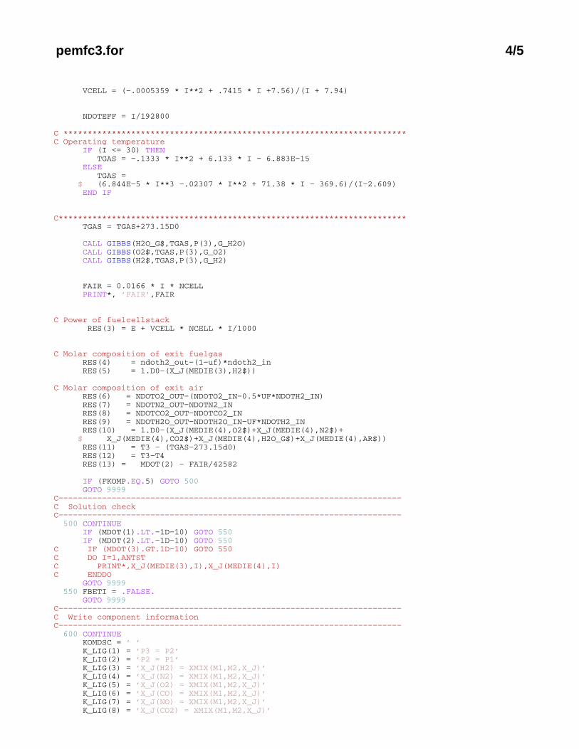
pemfc3.for 4/5

VCELL = (−.0005359 * I**2 + .7415 * I +7.56)/(I + 7.94)

NDOTEFF = I/192800

C ***********************************************************************C Operating temperature IF (I <= 30) THEN TGAS = −.1333 * I**2 + 6.133 * I − 6.883E−15 ELSE TGAS = $ (6.844E−5 * I**3 −.02307 * I**2 + 71.38 * I − 369.6)/(I−2.609) END IF

C************************************************************************ TGAS = TGAS+273.15D0

CALL GIBBS(H2O_G$,TGAS,P(3),G_H2O) CALL GIBBS(O2$,TGAS,P(3),G_O2) CALL GIBBS(H2$,TGAS,P(3),G_H2)

FAIR = 0.0166 * I * NCELL PRINT*, ’FAIR’,FAIR

C Power of fuelcellstack RES(3) = E + VCELL * NCELL * I/1000 C Molar composition of exit fuelgas RES(4) = ndoth2_out−(1−uf)*ndoth2_in RES(5) = 1.D0−(X_J(MEDIE(3),H2$))

C Molar composition of exit air RES(6) = NDOTO2_OUT−(NDOTO2_IN−0.5*UF*NDOTH2_IN) RES(7) = NDOTN2_OUT−NDOTN2_IN RES(8) = NDOTCO2_OUT−NDOTCO2_IN RES(9) = NDOTH2O_OUT−NDOTH2O_IN−UF*NDOTH2_IN RES(10) = 1.D0−(X_J(MEDIE(4),O2$)+X_J(MEDIE(4),N2$)+ $ X_J(MEDIE(4),CO2$)+X_J(MEDIE(4),H2O_G$)+X_J(MEDIE(4),AR$)) RES(11) = T3 − (TGAS−273.15d0) RES(12) = T3−T4 RES(13) = MDOT(2) − FAIR/42582 IF (FKOMP.EQ.5) GOTO 500 GOTO 9999C−−−−−−−−−−−−−−−−−−−−−−−−−−−−−−−−−−−−−−−−−−−−−−−−−−−−−−−−−−−−−−−−−−−−−−−C Solution checkC−−−−−−−−−−−−−−−−−−−−−−−−−−−−−−−−−−−−−−−−−−−−−−−−−−−−−−−−−−−−−−−−−−−−−−− 500 CONTINUE IF (MDOT(1).LT.−1D−10) GOTO 550 IF (MDOT(2).LT.−1D−10) GOTO 550C IF (MDOT(3).GT.1D−10) GOTO 550C DO I=1,ANTSTC PRINT*,X_J(MEDIE(3),I),X_J(MEDIE(4),I)C ENDDO GOTO 9999 550 FBETI = .FALSE. GOTO 9999C−−−−−−−−−−−−−−−−−−−−−−−−−−−−−−−−−−−−−−−−−−−−−−−−−−−−−−−−−−−−−−−−−−−−−−−C Write component informationC−−−−−−−−−−−−−−−−−−−−−−−−−−−−−−−−−−−−−−−−−−−−−−−−−−−−−−−−−−−−−−−−−−−−−−− 600 CONTINUE KOMDSC = ’ ’ K_LIG(1) = ’P3 = P2’ K_LIG(2) = ’P2 = P1’ K_LIG(3) = ’X_J(H2) = XMIX(M1,M2,X_J)’ K_LIG(4) = ’X_J(N2) = XMIX(M1,M2,X_J)’ K_LIG(5) = ’X_J(O2) = XMIX(M1,M2,X_J)’ K_LIG(6) = ’X_J(CO) = XMIX(M1,M2,X_J)’ K_LIG(7) = ’X_J(NO) = XMIX(M1,M2,X_J)’ K_LIG(8) = ’X_J(CO2) = XMIX(M1,M2,X_J)’

pemfc3.for 5/5

K_LIG(9) = ’X_J(H2O) = XMIX(M1,M2,X_J)’ K_LIG(10) = ’X_J(NH3) = XMIX(M1,M2,X_J)’ K_LIG(11) = ’X_J(H2S) = XMIX(M1,M2,X_J)’ K_LIG(12) = ’X_J(SO2) = XMIX(M1,M2,X_J)’ K_LIG(13) = ’X_J(CH4) = XMIX(M1,M2,X_J)’ K_LIG(14) = ’X_J(C2H6) = XMIX(M1,M2,X_J)’ K_LIG(15) = ’X_J(C3H8) = XMIX(M1,M2,X_J)’ K_LIG(16) = ’X_J(N−C4H10) = XMIX(M1,M2,X_J)’ K_LIG(17) = ’X_J(ISO−C4H10) = XMIX(M1,M2,X_J)’ K_LIG(18) = ’X_J(C5H12) = XMIX(M1,M2,X_J)’ K_LIG(19) = ’X_J(C6H14) = XMIX(M1,M2,X_J)’ K_LIG(20) = ’X_J(C7H16) = XMIX(M1,M2,X_J)’ K_LIG(21) = ’X_J(C8H18) = XMIX(M1,M2,X_J)’ K_LIG(22) = ’X_J(C2H4) = XMIX(M1,M2,X_J)’ K_LIG(23) = ’X_J(C3H6) = XMIX(M1,M2,X_J)’ K_LIG(24) = ’X_J(C5H10) = XMIX(M1,M2,X_J)’ K_LIG(25) = ’X_J(C6H12) = XMIX(M1,M2,X_J)’ K_LIG(26) = ’X_J(C7H14) = XMIX(M1,M2,X_J)’ K_LIG(27) = ’X_J(C2H2) = XMIX(M1,M2,X_J)’ K_LIG(28) = ’X_J(C6H6) = XMIX(M1,M2,X_J)’ K_LIG(29) = ’X_J(C6H12) = XMIX(M1,M2,X_J)’ K_LIG(30) = ’X_J(C) = XMIX(M1,M2,X_J)’ K_LIG(31) = ’X_J(S) = XMIX(M1,M2,X_J)’ K_LIG(32) = ’X_J(NO2) = XMIX(M1,M2,X_J)’ K_LIG(33) = ’X_J(HCN) = XMIX(M1,M2,X_J)’ K_LIG(34) = ’X_J(COS) = XMIX(M1,M2,X_J)’ K_LIG(35) = ’X_J(N2O) = XMIX(M1,M2,X_J)’ K_LIG(36) = ’X_J(NO3) = XMIX(M1,M2,X_J)’ K_LIG(37) = ’X_J(SO3) = XMIX(M1,M2,X_J)’ K_LIG(38) = ’X_J(AR) = XMIX(M1,M2,X_J)’ K_LIG(39) = ’X_J(SiO2) = XMIX(M1,M2,X_J)’ K_BET = ’MDOT1 \\gt 0 $ MDOT2 \\gt 0 $ MDOT3 \\lt 0’ K_PAR(1) = ’ ’ K_MED(1) = MEDIE(1) K_MED(2) = MEDIE(2) K_MED(3) = MEDIE(3) KMEDDS(1) = ’ ’ KMEDDS(2) = ’ ’ KMEDDS(3) = ’ ’ KMEDDS(4) = ’ ’ KMEDDS(5) = ’ ’ KMEDDS(6) = ’ ’

CALL COMINF(KOMTY,KOMDSC,1,1,1,1, $ K_MED,K_PAR,K_LIG,K_BET,KMEDDS,K_STAT,K_INP,K_GRAF) GOTO 9999C 9999 CONTINUE RETURN END

C=======================================================================C=======================================================================

A.4 The source code of PEMFC component model basedon electrochemical reactions

132

pemfc0D_EH2.for 1/8

C*********************************************************************** SUBROUTINE PEMFC0D_EH2 (KOMTY,ANTLK,ANTEX,ANTED,ANTKN,ANTPK,ANTM1, : ANTM2,ANTSW,DYCOM,MEDIE,ANTME,VARME,ANTEL, : VAREL,MDOT,P,H,E,Q,PAR,RES,X_J)C***********************************************************************CC PEMFC1 is a model of a PEM Fuel Cell. The equations are based on C Theoretical and semi−empirical expressions.

C***********************************************************************CCA FKOMP − INPUT − Flag with the value:CA 1: Initialize the component.CA 2: Initialize with actual system.CA 3: Fluid composition calculation (constant).CA 4: Find residuals.CA 5: Find residuals and check variables.CA 6: Output information about component.CA MDOT − INPUT − Massflows from nodes.CA P − INPUT − Pressure in nodes.CA X_J − INPUT − Fluid composition.CA KOMTY − OUTPUT − Component name.CA ANTPK − OUTPUT − Number of parameters for the component.CA ANTLK − OUTPUT − Number of equations in the component.CA ANTEX − OUTPUT − Number of independent equations in the component.CA ANTED − OUTPUT − Number of differential independent equations.CA ANTKN − OUTPUT − Number of nodes connected to the component.CA ANTM1 − OUTPUT − Number of massflows in the first conservation ofCA mass equation.CA ANTM2 − OUTPUT − Number of massflows in the second.CA DYCOM − OUTPUT − Type of conservation equations (static or dynamicCA mass and internal energy on side 1 and 2 respectively;CA and dynamic solid internal energy).CA MEDIE − IN/OUT − Media (fluid) of the connected nodes.CA The values mean :CA CA −4 : Any gasCA ANTME − OUTPUT − Number of fluids with variable composition.CA VARME − OUTPUT − Pointer to fluid numbers (with variable composition).CA ANTEL − OUTPUT − Number of computed compounds in these variable fluids.CA VAREL − OUTPUT − Compound numbers in variable fluids.CA RES − OUTPUT − Residuals for the component.CCL XMIX Composition of the mixture.CL K_PAR Parameter description.CL K_LIG Equation description.CL K_BET Condition description.CL K_MED Media description.CC Subroutines : COMINFC CCP Programmer : Elham Hosseinzadeh (ehos), TES, MEK, DTU, 2012

C***********************************************************************CC Including the common "environment"C INCLUDE ’ENVIRO.INI’ INCLUDE ’THERPROP.DEC’CC Parameter variablesC INTEGER ANTLK, ANTEX, ANTED, ANTKN, MEDIE(6), ANTPK, : ANTM1, ANTM2,ANTSW, ANTME, VARME(4), ANTEL(4), : VAREL(ANTST,4),NCELL DOUBLE PRECISION X_J(MAXME,ANTST), RES(14),MDOT(4),P(4), : H(4),E,Q(1),PAR(7) CHARACTER*3 DYCOM(5) CHARACTER*80 KOMTYCC Local variablesC INTEGER K_MED(6)

pemfc0D_EH2.for 2/8

DOUBLE PRECISION NDOTH2_IN,NDOTCO2_IN, $ NDOTH2O_IN,NDOTO2_IN,NDOTN2_IN,NDOTAR_IN,NDOTN2_OUT, $ NDOTH2_OUT,NDOTO2_OUT, NDOTCO2_OUT,NDOTH2O_OUT, $ NDOTAR_OUT,XH2_IN,XCO2_IN,XH2O_IN,XO2_IN,XN2_IN,XAR_IN, $ XH2_OUT,XCO2_OUT,XH2O_OUT,XO2_OUT,XN2_OUT,XAR_OUT, $ M_BR_IN,M_AIR_IN,ETASYS,M_BR_OUT,M_AIR_OUT,T3,T4,TGAS, $ V,S,X,DUM,G_H2,G_O2,G_H2O,GMAX, etamax,VCELL,DP1,DP2,R, $ P_anode,P_cathode,Far,I_total,P_standard,G_standard,E_nernst, $ i0_a,i0_c,V_act_a,V_act_c,V_act,sigma,tm,Landa,RH,R_ionic, $ R_elec,V_ohmic,V_cell,P_O2,G_real,Landa_a,Landa_c,aw_a,aw_c, $ P_H2O_a,P_H2O_c,aa,bb,cc,dd,ee,ff,P_vs,landa_z,JH2O_a,JH2O_c, $ Ro_dry,Mm,D_landa,J_net_n,J_net_m,J_net_flux, MDOTH2O_a, $ MH2O_OUT,NH2O_OUT,NDOTH2O_IN_a,NDOTH2O_OUT_a,i_cd,aaa, bbb, $ PH2O_c_in,PH2O_c_out,XH2O_OUT_a,XH2O_IN_a, A_cell,SH2,SAIR, $ P_vs_in,T2,T1, R_ionic_ohm,i_n,I_cell,Pa_vs_in,PH2O_a_in, $ PH2O_a_out,DX,P_H2_in,P_H2_out,P_H2, zeta1,zeta2,zeta3,zeta4, $ C_O2,il_H2,il_O2,il_min,V_conc,V_conc_cathode,V_conc_anode, $ MDOT_VAP_C,MDOT_LIQ_C,MDOT_VAP_A,MDOT_LIQ_A,landa_ave, na,nc, $ B,A_a,A_c

CHARACTER*100 K_PAR(1),K_STAT(1) CHARACTER*500 K_LIG(39), K_BET, KOMDSC,K_INP,K_GRAF CHARACTER*100 KMEDDS(6) EXTERNAL COMINF INCLUDE ’THERPROP.INI’

C======================================================================= GOTO (100,200,300,400,400,200) FKOMP RETURN

C−−−−−−−−−−−−−−−−−−−−−−−−−−−−−−−−−−−−−−−−−−−−−−−−−−−−−−−−−−−−−−−−−−−−−−−C Component nameC−−−−−−−−−−−−−−−−−−−−−−−−−−−−−−−−−−−−−−−−−−−−−−−−−−−−−−−−−−−−−−−−−−−−−−− 100 CONTINUE KOMTY = ’PEMFC0D_EH2’

GOTO 9999C−−−−−−−−−−−−−−−−−−−−−−−−−−−−−−−−−−−−−−−−−−−−−−−−−−−−−−−−−−−−−−−−−−−−−−−C Component characteristicsC−−−−−−−−−−−−−−−−−−−−−−−−−−−−−−−−−−−−−−−−−−−−−−−−−−−−−−−−−−−−−−−−−−−−−−− 200 CONTINUE KOMTY = ’PEMFC0D_EH2’ ANTKN = 6 ANTPK = 7 ANTLK = 14 ANTM1 = 4 MEDIE(1) = ANYGAS$ MEDIE(2) = ANYGAS$ MEDIE(3) = ANYGAS$ MEDIE(4) = ANYGAS$ MEDIE(5) = POWER$ MEDIE(6) = HEAT$ ANTME = 4 VARME(1) = NODE1$ VARME(2) = NODE2$ VARME(3) = NODE3$c ANTEL(3) = 1 ANTEL(3) = 2 VARME(4) = NODE4$ ANTEL(4) = 5 VAREL(1,3)=H2$ VAREL(2,3)=H2O_G$ VAREL(1,4)=O2$ VAREL(2,4)=N2$ VAREL(3,4)=CO2$ VAREL(4,4)=H2O_G$ VAREL(5,4)=AR$ IF (FKOMP.EQ.6) GOTO 600 GOTO 9999C−−−−−−−−−−−−−−−−−−−−−−−−−−−−−−−−−−−−−−−−−−−−−−−−−−−−−−−−−−−−−−−−−−−−−−−C Fluid composition calculation (constant).C−−−−−−−−−−−−−−−−−−−−−−−−−−−−−−−−−−−−−−−−−−−−−−−−−−−−−−−−−−−−−−−−−−−−−−− 300 CONTINUE

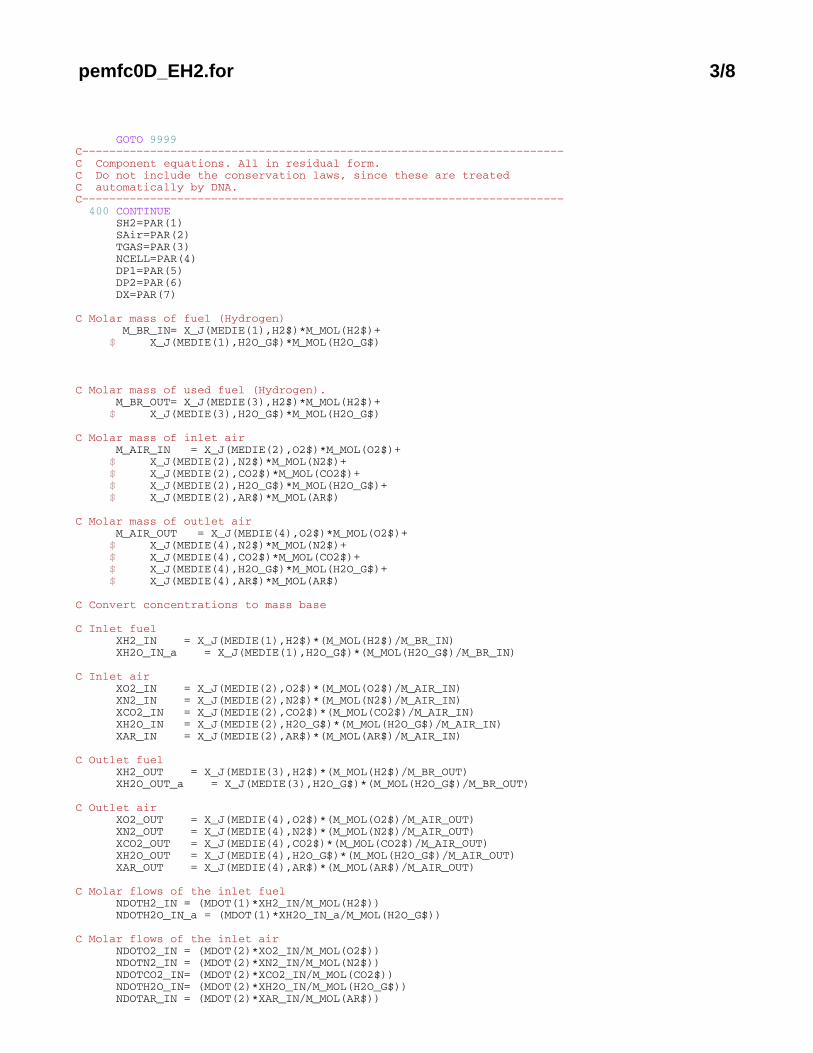
pemfc0D_EH2.for 3/8

GOTO 9999C−−−−−−−−−−−−−−−−−−−−−−−−−−−−−−−−−−−−−−−−−−−−−−−−−−−−−−−−−−−−−−−−−−−−−−−C Component equations. All in residual form.C Do not include the conservation laws, since these are treatedC automatically by DNA.C−−−−−−−−−−−−−−−−−−−−−−−−−−−−−−−−−−−−−−−−−−−−−−−−−−−−−−−−−−−−−−−−−−−−−−− 400 CONTINUE SH2=PAR(1) SAir=PAR(2) TGAS=PAR(3) NCELL=PAR(4) DP1=PAR(5) DP2=PAR(6) DX=PAR(7) C Molar mass of fuel (Hydrogen) M_BR_IN= X_J(MEDIE(1),H2$)*M_MOL(H2$)+ $ X_J(MEDIE(1),H2O_G$)*M_MOL(H2O_G$)

C Molar mass of used fuel (Hydrogen). M_BR_OUT= X_J(MEDIE(3),H2$)*M_MOL(H2$)+ $ X_J(MEDIE(3),H2O_G$)*M_MOL(H2O_G$) C Molar mass of inlet air M_AIR_IN = X_J(MEDIE(2),O2$)*M_MOL(O2$)+ $ X_J(MEDIE(2),N2$)*M_MOL(N2$)+ $ X_J(MEDIE(2),CO2$)*M_MOL(CO2$)+ $ X_J(MEDIE(2),H2O_G$)*M_MOL(H2O_G$)+ $ X_J(MEDIE(2),AR$)*M_MOL(AR$)

C Molar mass of outlet air M_AIR_OUT = X_J(MEDIE(4),O2$)*M_MOL(O2$)+ $ X_J(MEDIE(4),N2$)*M_MOL(N2$)+ $ X_J(MEDIE(4),CO2$)*M_MOL(CO2$)+ $ X_J(MEDIE(4),H2O_G$)*M_MOL(H2O_G$)+ $ X_J(MEDIE(4),AR$)*M_MOL(AR$)

C Convert concentrations to mass base

C Inlet fuel XH2_IN = X_J(MEDIE(1),H2$)*(M_MOL(H2$)/M_BR_IN) XH2O_IN_a = X_J(MEDIE(1),H2O_G$)*(M_MOL(H2O_G$)/M_BR_IN)

C Inlet air XO2_IN = X_J(MEDIE(2),O2$)*(M_MOL(O2$)/M_AIR_IN) XN2_IN = X_J(MEDIE(2),N2$)*(M_MOL(N2$)/M_AIR_IN) XCO2_IN = X_J(MEDIE(2),CO2$)*(M_MOL(CO2$)/M_AIR_IN) XH2O_IN = X_J(MEDIE(2),H2O_G$)*(M_MOL(H2O_G$)/M_AIR_IN) XAR_IN = X_J(MEDIE(2),AR$)*(M_MOL(AR$)/M_AIR_IN)

C Outlet fuel XH2_OUT = X_J(MEDIE(3),H2$)*(M_MOL(H2$)/M_BR_OUT) XH2O_OUT_a = X_J(MEDIE(3),H2O_G$)*(M_MOL(H2O_G$)/M_BR_OUT)

C Outlet air XO2_OUT = X_J(MEDIE(4),O2$)*(M_MOL(O2$)/M_AIR_OUT) XN2_OUT = X_J(MEDIE(4),N2$)*(M_MOL(N2$)/M_AIR_OUT) XCO2_OUT = X_J(MEDIE(4),CO2$)*(M_MOL(CO2$)/M_AIR_OUT) XH2O_OUT = X_J(MEDIE(4),H2O_G$)*(M_MOL(H2O_G$)/M_AIR_OUT) XAR_OUT = X_J(MEDIE(4),AR$)*(M_MOL(AR$)/M_AIR_OUT)

C Molar flows of the inlet fuel NDOTH2_IN = (MDOT(1)*XH2_IN/M_MOL(H2$)) NDOTH2O_IN_a = (MDOT(1)*XH2O_IN_a/M_MOL(H2O_G$))

C Molar flows of the inlet air NDOTO2_IN = (MDOT(2)*XO2_IN/M_MOL(O2$)) NDOTN2_IN = (MDOT(2)*XN2_IN/M_MOL(N2$)) NDOTCO2_IN= (MDOT(2)*XCO2_IN/M_MOL(CO2$)) NDOTH2O_IN= (MDOT(2)*XH2O_IN/M_MOL(H2O_G$)) NDOTAR_IN = (MDOT(2)*XAR_IN/M_MOL(AR$))

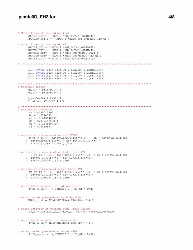
pemfc0D_EH2.for 4/8

C Molar flows of the outlet fuel NDOTH2_OUT = −(MDOT(3)*XH2_OUT/M_MOL(H2$)) NDOTH2O_OUT_a = −(MDOT(3)*XH2O_OUT_a/M_MOL(H2O_G$))

C Molar flows of the outlet air NDOTO2_OUT = −(MDOT(4)*XO2_OUT/M_MOL(O2$)) NDOTN2_OUT = −(MDOT(4)*XN2_OUT/M_MOL(N2$)) NDOTCO2_OUT= −(MDOT(4)*XCO2_OUT/M_MOL(CO2$)) NDOTH2O_OUT= −(MDOT(4)*XH2O_OUT/M_MOL(H2O_G$)) NDOTAR_OUT = −(MDOT(4)*XAR_OUT/M_MOL(AR$))

C *********************************************************************************

CALL STATES(P(1),H(1),T1,V,S,X,DUM,1,2,MEDIE(1)) CALL STATES(P(2),H(2),T2,V,S,X,DUM,1,2,MEDIE(2)) CALL STATES(P(3),H(3),T3,V,S,X,DUM,1,2,MEDIE(3)) CALL STATES(P(4),H(4),T4,V,S,X,DUM,1,2,MEDIE(4))

***********************************************************************************c Pressure losses RES(1) = p(1)−DP1−P(3) RES(2) = p(2)−DP2−P(4)

P_anode=(P(1)+P(3))/2 P_cathode=(P(2)+P(4))/2

C *********************************************************************************c Saturation Pressure aa = −5800.2206 bb = 1.3914993 cc = −0.048640239 dd = 0.41764768D−4 ee = −0.14452093D−7 ff = 6.5459673

c saturation pressure of outlet (TGAS) P_vs = (EXP( (aa*(TGAS+273.15)**(−1)) + bb + cc*(TGAS+273.15) + $ dd*(TGAS+273.15)**2 + ee*(TGAS+273.15)**3 + $ ff*log(TGAS+273.15))) /1D5

c saturation pressure of cathode inlet (T2) P_vs_in = (EXP( (aa*(T2+273.15)**(−1)) + bb + cc*(T2+273.15) + $ dd*(T2+273.15)**2 + ee*(T2+273.15)**3 + $ ff*log(T2+273.15))) /1D5

c saturation pressure of anode inlet (T1) Pa_vs_in = (EXP( (aa*(T1+273.15)**(−1)) + bb + cc*(T1+273.15) + $ dd*(T1+273.15)**2 + ee*(T1+273.15)**3 + $ ff*log(T1+273.15))) /1D5

c water inlet pressure at cathode side PH2O_c_in = X_J(MEDIE(2),H2O_G$)* P(2)

c water oultel pressure at cathode side PH2O_c_out = (X_J(MEDIE(4),H2O_G$)* P(4))

c water activity at cathode side (mean value) aw_c = DX*(PH2O_c_in/P_vs_in)+(1−DX)*(PH2O_c_out/P_vs)

c water inlet pressure at anode side PH2O_a_in = (X_J(MEDIE(1),H2O_G$)* P(1))

c watre outlet pressure at anode side PH2O_a_out = (X_J(MEDIE(3),H2O_G$)* P(3))

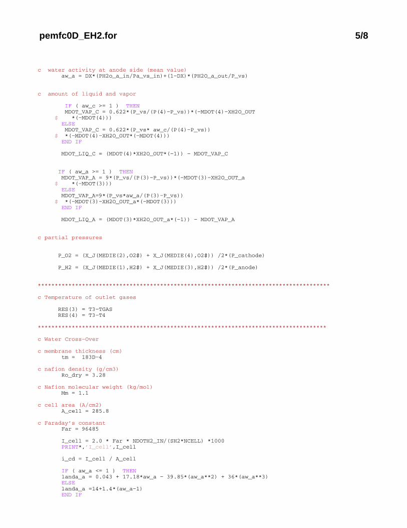
pemfc0D_EH2.for 5/8

c water activity at anode side (mean value) aw_a = DX*(PH2o_a_in/Pa_vs_in)+(1−DX)*(PH2O_a_out/P_vs)

c amount of liquid and vapor

IF ( aw_c >= 1 ) THEN MDOT_VAP_C = 0.622*(P_vs/(P(4)−P_vs))*(−MDOT(4)−XH2O_OUT $ *(−MDOT(4))) ELSE MDOT_VAP_C = 0.622*(P_vs* aw_c/(P(4)−P_vs)) $ *(−MDOT(4)−XH2O_OUT*(−MDOT(4))) END IF

MDOT_LIQ_C = (MDOT(4)*XH2O_OUT*(−1)) − MDOT_VAP_C

IF ( aw_a >= 1 ) THEN MDOT_VAP_A = 9*(P_vs/(P(3)−P_vs))*(−MDOT(3)−XH2O_OUT_a $ *(−MDOT(3))) ELSE MDOT_VAP_A=9*(P_vs*aw_a/(P(3)−P_vs)) $ *(−MDOT(3)−XH2O_OUT_a*(−MDOT(3))) END IF

MDOT_LIQ_A = (MDOT(3)*XH2O_OUT_a*(−1)) − MDOT_VAP_A

c partial pressures

P_O2 = (X_J(MEDIE(2),O2$) + X_J(MEDIE(4),O2$)) /2*(P_cathode)

P_H2 = (X_J(MEDIE(1),H2$) + X_J(MEDIE(3),H2$)) /2*(P_anode)

**************************************************************************************

c Temperature of outlet gases

RES(3) = T3−TGAS RES(4) = T3−T4

*************************************************************************************

c Water Cross−Over

c membrane thickness (cm) tm = 183D−4

c nafion density (g/cm3) Ro_dry = 3.28

c Nafion molecular weight (kg/mol) Mm = 1.1 c cell area (A/cm2) A_cell = 285.8

c Faraday’s constant Far = 96485

I_cell = 2.0 * Far * NDOTH2_IN/(SH2*NCELL) *1000 PRINT*,’I_cell’,I_cell i_cd = I_cell / A_cell

IF ( aw_a <= 1 ) THEN landa_a = 0.043 + 17.18*aw_a − 39.85*(aw_a**2) + 36*(aw_a**3) ELSE landa_a =14+1.4*(aw_a−1) END IF

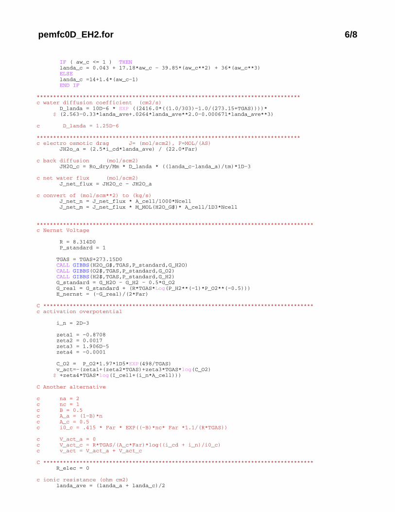
pemfc0D_EH2.for 6/8

IF ( aw_c <= 1 ) THEN landa_c = 0.043 + 17.18*aw_c − 39.85*(aw_c**2) + 36*(aw_c**3) ELSE landa_c =14+1.4*(aw_c−1) END IF ********************************************************************************c water diffusion coefficient (cm2/s) D_landa = 10D−6 * EXP ((2416.0*((1.0/303)−1.0/(273.15+TGAS))))* $ (2.563−0.33*landa_ave+.0264*landa_ave**2.0−0.000671*landa_ave**3)

c D_landa = 1.25D−6 ********************************************************************************c electro osmotic drag J= (mol/scm2), F=MOL/(AS) JH2o_a = (2.5*i_cd*landa_ave) / (22.0*Far)

c back diffusion (mol/scm2) JH2O_c = Ro_dry/Mm * D_landa * ((landa_c−landa_a)/tm)*1D−3

c net water flux (mol/scm2) J_net_flux = JH2O_c − JH2O_a

c convert of (mol/scm**2) to (kg/s) J_net_n = J_net_flux * A_cell/1000*Ncell J_net_m = J_net_flux * M_MOL(H2O_G$)* A_cell/1D3*Ncell

************************************************************************************c Nernst Voltage R = 8.314D0 P_standard = 1 TGAS = TGAS+273.15D0 CALL GIBBS(H2O_G$,TGAS,P_standard,G_H2O) CALL GIBBS(O2$,TGAS,P_standard,G_O2) CALL GIBBS(H2$,TGAS,P_standard,G_H2) G_standard = G_H2O − G_H2 − 0.5*G_O2 G_real = G_standard + (R*TGAS*Log(P_H2**(−1)*P_O2**(−0.5))) E_nernst = (−G_real)/(2*Far)

C ********************************************************************************** c activation overpotential

i_n = 2D−3 zeta1 = −0.8708 zeta2 = 0.0017 zeta3 = 1.906D−5 zeta4 = −0.0001

C_O2 = P_O2*1.97*1D5*EXP(498/TGAS) v_act=−(zeta1+(zeta2*TGAS)+zeta3*TGAS*log(C_O2) $ +zeta4*TGAS*log(I_cell+(i_n*A_cell)))

C Another alternative

c na = 2c nc = 1c B = 0.5c A_a = (1−B)*nc A_c = 0.5c i0_c = .415 * Far * EXP((−B)*nc* Far *1.1/(R*TGAS))

c V_act_a = 0c V_act_c = R*TGAS/(A_c*Far)*log((i_cd + i_n)/i0_c)c v_act = V_act_a + V_act_c

C ********************************************************************************** R_elec = 0

c ionic resistance (ohm cm2) landa_ave = (landa_a + landa_c)/2

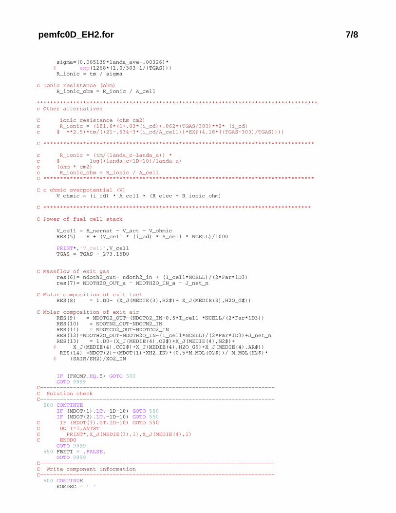
pemfc0D_EH2.for 7/8

sigma=(0.005139*landa_ave−.00326)* $ exp(1268*(1.0/303−1/(TGAS))) R_ionic = tm / sigma c Ionic resistance (ohm) R_ionic_ohm = R_ionic / A_cell

*************************************************************************************c Other alternatives

C ionic resistance (ohm cm2)c R_ionic = (181.6*(1+.03*(i_cd)+.062*(TGAS/303)**2* (i_cd)c $ **2.5)*tm/((21−.634−3*(i_cd/A_cell))*EXP(4.18*((TGAS−303)/TGAS))))

C **********************************************************************************

c R_ionic = (tm/(landa_c−landa_a)) * c $ log((landa_c+1D−10)/landa_a)c (ohm * cm2)c R_ionic_ohm = R_ionic / A_cell C **********************************************************************************

C c ohmic overpotential (V) V_ohmic = (i_cd) * A_cell * (R_elec + R_ionic_ohm)

C *********************************************************************************

C Power of fuel cell stack

V_cell = E_nernst − V_act − V_ohmic RES(5) = E + (V_cell * (i_cd) * A_cell * NCELL)/1000

PRINT*,’V_cell’,V_cell TGAS = TGAS − 273.15D0

C Massflow of exit gas res(6)= ndoth2_out− ndoth2_in + (I_cell*NCELL)/(2*Far*1D3) res(7)= NDOTH2O_OUT_a − NDOTH2O_IN_a − J_net_n

C Molar composition of exit fuel RES(8) = 1.D0− (X_J(MEDIE(3),H2$)+ X_J(MEDIE(3),H2O_G$))

C Molar composition of exit air RES(9) = NDOTO2_OUT−(NDOTO2_IN−0.5*I_cell *NCELL/(2*Far*1D3)) RES(10) = NDOTN2_OUT−NDOTN2_IN RES(11) = NDOTCO2_OUT−NDOTCO2_IN RES(12)=NDOTH2O_OUT−NDOTH2O_IN−(I_cell*NCELL)/(2*Far*1D3)+J_net_n RES(13) = 1.D0−(X_J(MEDIE(4),O2$)+X_J(MEDIE(4),N2$)+ $ X_J(MEDIE(4),CO2$)+X_J(MEDIE(4),H2O_G$)+X_J(MEDIE(4),AR$)) RES(14) =MDOT(2)−(MDOT(1)*XH2_IN)*(0.5*M_MOL(O2$))/ M_MOL(H2$)* $ (SAIR/SH2)/XO2_IN

IF (FKOMP.EQ.5) GOTO 500 GOTO 9999C−−−−−−−−−−−−−−−−−−−−−−−−−−−−−−−−−−−−−−−−−−−−−−−−−−−−−−−−−−−−−−−−−−−−−−−C Solution checkC−−−−−−−−−−−−−−−−−−−−−−−−−−−−−−−−−−−−−−−−−−−−−−−−−−−−−−−−−−−−−−−−−−−−−−− 500 CONTINUE IF (MDOT(1).LT.−1D−10) GOTO 550 IF (MDOT(2).LT.−1D−10) GOTO 550C IF (MDOT(3).GT.1D−10) GOTO 550C DO I=1,ANTSTC PRINT*,X_J(MEDIE(3),I),X_J(MEDIE(4),I)C ENDDO GOTO 9999 550 FBETI = .FALSE. GOTO 9999C−−−−−−−−−−−−−−−−−−−−−−−−−−−−−−−−−−−−−−−−−−−−−−−−−−−−−−−−−−−−−−−−−−−−−−−C Write component informationC−−−−−−−−−−−−−−−−−−−−−−−−−−−−−−−−−−−−−−−−−−−−−−−−−−−−−−−−−−−−−−−−−−−−−−− 600 CONTINUE KOMDSC = ’ ’

pemfc0D_EH2.for 8/8

K_LIG(1) = ’P3 = P2’ K_LIG(2) = ’P2 = P1’ K_LIG(3) = ’X_J(H2) = XMIX(M1,M2,X_J)’ K_LIG(4) = ’X_J(N2) = XMIX(M1,M2,X_J)’ K_LIG(5) = ’X_J(O2) = XMIX(M1,M2,X_J)’ K_LIG(6) = ’X_J(CO) = XMIX(M1,M2,X_J)’ K_LIG(7) = ’X_J(NO) = XMIX(M1,M2,X_J)’ K_LIG(8) = ’X_J(CO2) = XMIX(M1,M2,X_J)’ K_LIG(9) = ’X_J(H2O) = XMIX(M1,M2,X_J)’ K_LIG(10) = ’X_J(NH3) = XMIX(M1,M2,X_J)’ K_LIG(11) = ’X_J(H2S) = XMIX(M1,M2,X_J)’ K_LIG(12) = ’X_J(SO2) = XMIX(M1,M2,X_J)’ K_LIG(13) = ’X_J(CH4) = XMIX(M1,M2,X_J)’ K_LIG(14) = ’X_J(C2H6) = XMIX(M1,M2,X_J)’ K_LIG(15) = ’X_J(C3H8) = XMIX(M1,M2,X_J)’ K_LIG(16) = ’X_J(N−C4H10) = XMIX(M1,M2,X_J)’ K_LIG(17) = ’X_J(ISO−C4H10) = XMIX(M1,M2,X_J)’ K_LIG(18) = ’X_J(C5H12) = XMIX(M1,M2,X_J)’ K_LIG(19) = ’X_J(C6H14) = XMIX(M1,M2,X_J)’ K_LIG(20) = ’X_J(C7H16) = XMIX(M1,M2,X_J)’ K_LIG(21) = ’X_J(C8H18) = XMIX(M1,M2,X_J)’ K_LIG(22) = ’X_J(C2H4) = XMIX(M1,M2,X_J)’ K_LIG(23) = ’X_J(C3H6) = XMIX(M1,M2,X_J)’ K_LIG(24) = ’X_J(C5H10) = XMIX(M1,M2,X_J)’ K_LIG(25) = ’X_J(C6H12) = XMIX(M1,M2,X_J)’ K_LIG(26) = ’X_J(C7H14) = XMIX(M1,M2,X_J)’ K_LIG(27) = ’X_J(C2H2) = XMIX(M1,M2,X_J)’ K_LIG(28) = ’X_J(C6H6) = XMIX(M1,M2,X_J)’ K_LIG(29) = ’X_J(C6H12) = XMIX(M1,M2,X_J)’ K_LIG(30) = ’X_J(C) = XMIX(M1,M2,X_J)’ K_LIG(31) = ’X_J(S) = XMIX(M1,M2,X_J)’ K_LIG(32) = ’X_J(NO2) = XMIX(M1,M2,X_J)’ K_LIG(33) = ’X_J(HCN) = XMIX(M1,M2,X_J)’ K_LIG(34) = ’X_J(COS) = XMIX(M1,M2,X_J)’ K_LIG(35) = ’X_J(N2O) = XMIX(M1,M2,X_J)’ K_LIG(36) = ’X_J(NO3) = XMIX(M1,M2,X_J)’ K_LIG(37) = ’X_J(SO3) = XMIX(M1,M2,X_J)’ K_LIG(38) = ’X_J(AR) = XMIX(M1,M2,X_J)’ K_LIG(39) = ’X_J(SiO2) = XMIX(M1,M2,X_J)’ K_BET = ’MDOT1 \\gt 0 $ MDOT2 \\gt 0 $ MDOT3 \\lt 0’ K_PAR(1) = ’ ’ K_MED(1) = MEDIE(1) K_MED(2) = MEDIE(2) K_MED(3) = MEDIE(3) KMEDDS(1) = ’ ’ KMEDDS(2) = ’ ’ KMEDDS(3) = ’ ’ KMEDDS(4) = ’ ’ KMEDDS(5) = ’ ’ KMEDDS(6) = ’ ’

CALL COMINF(KOMTY,KOMDSC,1,1,1,1, $ K_MED,K_PAR,K_LIG,K_BET,KMEDDS,K_STAT,K_INP,K_GRAF) GOTO 9999C 9999 CONTINUE RETURN END

C=======================================================================C=======================================================================

A.5 Flow sheet of PEMFC component model with nodenumbers

141

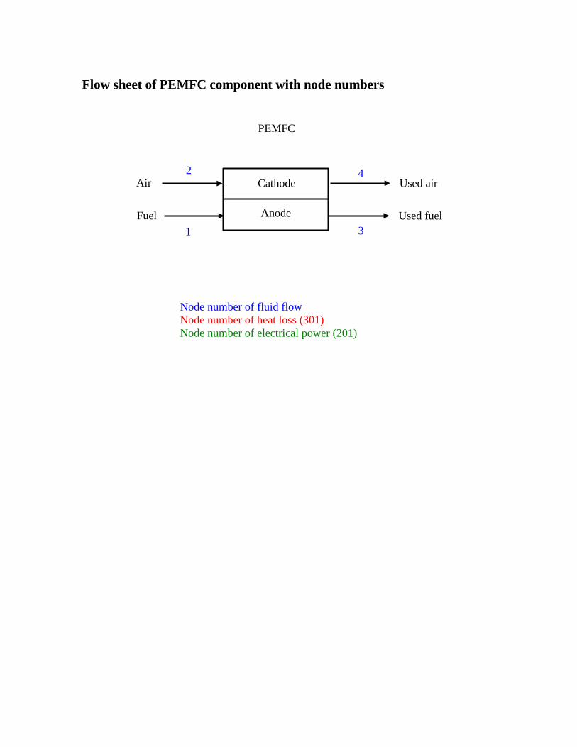
Cathode

Anode

PEMFC

Air Used air

Fuel Used fuel

Node number of fluid flow Node number of heat loss (301) Node number of electrical power (201)

2

1

3

4

Flow sheet of PEMFC component with node numbers

A.6 DNA Input for PEMFC system

143

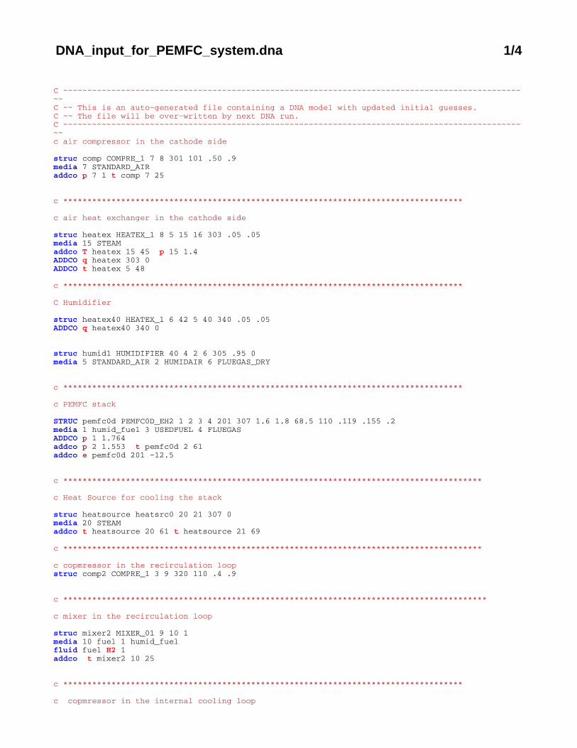
DNA_input_for_PEMFC_system.dna 1/4

C ~~~~~~~~~~~~~~~~~~~~~~~~~~~~~~~~~~~~~~~~~~~~~~~~~~~~~~~~~~~~~~~~~~~~~~~~~~~~~~~~~~~~~~~~~~~~~~~~~C ~~ This is an auto−generated file containing a DNA model with updated initial guesses. C ~~ The file will be over−written by next DNA run.C ~~~~~~~~~~~~~~~~~~~~~~~~~~~~~~~~~~~~~~~~~~~~~~~~~~~~~~~~~~~~~~~~~~~~~~~~~~~~~~~~~~~~~~~~~~~~~~~~~c air compressor in the cathode side struc comp COMPRE_1 7 8 301 101 .50 .9media 7 STANDARD_AIRaddco p 7 1 t comp 7 25

c *********************************************************************************** c air heat exchanger in the cathode side struc heatex HEATEX_1 8 5 15 16 303 .05 .05media 15 STEAMaddco T heatex 15 45 p 15 1.4ADDCO q heatex 303 0ADDCO t heatex 5 48 c *********************************************************************************** C Humidifier struc heatex40 HEATEX_1 6 42 5 40 340 .05 .05ADDCO q heatex40 340 0

struc humid1 HUMIDIFIER 40 4 2 6 305 .95 0media 5 STANDARD_AIR 2 HUMIDAIR 6 FLUEGAS_DRY

c *********************************************************************************** c PEMFC stack STRUC pemfc0d PEMFC0D_EH2 1 2 3 4 201 307 1.6 1.8 68.5 110 .119 .155 .2media 1 humid_fuel 3 USEDFUEL 4 FLUEGAS ADDCO p 1 1.764addco p 2 1.553 t pemfc0d 2 61addco e pemfc0d 201 −12.5 c *************************************************************************************** c Heat Source for cooling the stack struc heatsource heatsrc0 20 21 307 0media 20 STEAMaddco t heatsource 20 61 t heatsource 21 69 c *************************************************************************************** c copmressor in the recirculation loopstruc comp2 COMPRE_1 3 9 320 110 .4 .9

c **************************************************************************************** c mixer in the recirculation loop struc mixer2 MIXER_01 9 10 1media 10 fuel 1 humid_fuelfluid fuel H2 1addco t mixer2 10 25

c *********************************************************************************** c copmressor in the internal cooling loop

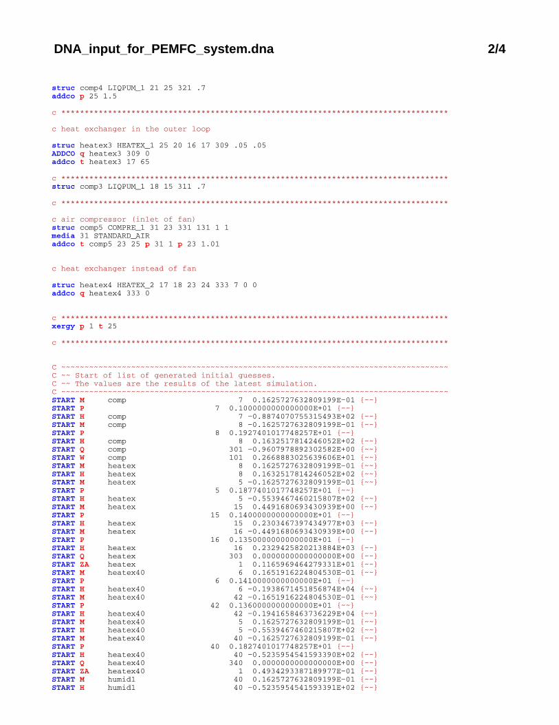
DNA_input_for_PEMFC_system.dna 2/4

struc comp4 LIQPUM_1 21 25 321 .7addco p 25 1.5 c *********************************************************************************** c heat exchanger in the outer loop struc heatex3 HEATEX_1 25 20 16 17 309 .05 .05ADDCO q heatex3 309 0addco t heatex3 17 65 c ***********************************************************************************struc comp3 LIQPUM_1 18 15 311 .7 c *********************************************************************************** c air compressor (inlet of fan)struc comp5 COMPRE_1 31 23 331 131 1 1media 31 STANDARD_AIRaddco t comp5 23 25 p 31 1 p 23 1.01

c heat exchanger instead of fan struc heatex4 HEATEX_2 17 18 23 24 333 7 0 0addco q heatex4 333 0

c ***********************************************************************************xergy p 1 t 25 c *********************************************************************************** C ~~~~~~~~~~~~~~~~~~~~~~~~~~~~~~~~~~~~~~~~~~~~~~~~~~~~~~~~~~~~~~~~~~~~~~~~~~~~~~~~~~~C ~~ Start of list of generated initial guesses.C ~~ The values are the results of the latest simulation.C ~~~~~~~~~~~~~~~~~~~~~~~~~~~~~~~~~~~~~~~~~~~~~~~~~~~~~~~~~~~~~~~~~~~~~~~~~~~~~~~~~~~START M comp 7 0.1625727632809199E−01 ~~START P 7 0.1000000000000000E+01 ~~START H comp 7 −0.8874070755315493E+02 ~~START M comp 8 −0.1625727632809199E−01 ~~START P 8 0.1927401017748257E+01 ~~START H comp 8 0.1632517814246052E+02 ~~START Q comp 301 −0.9607978892302582E+00 ~~START W comp 101 0.2668883025639606E+01 ~~START M heatex 8 0.1625727632809199E−01 ~~START H heatex 8 0.1632517814246052E+02 ~~START M heatex 5 −0.1625727632809199E−01 ~~START P 5 0.1877401017748257E+01 ~~START H heatex 5 −0.5539467460215807E+02 ~~START M heatex 15 0.4491680693430939E+00 ~~START P 15 0.1400000000000000E+01 ~~START H heatex 15 0.2303467397434977E+03 ~~START M heatex 16 −0.4491680693430939E+00 ~~START P 16 0.1350000000000000E+01 ~~START H heatex 16 0.2329425820213884E+03 ~~START Q heatex 303 0.0000000000000000E+00 ~~START ZA heatex 1 0.1165969464279331E+01 ~~START M heatex40 6 0.1651916224804530E−01 ~~START P 6 0.1410000000000000E+01 ~~START H heatex40 6 −0.1938671451856874E+04 ~~START M heatex40 42 −0.1651916224804530E−01 ~~START P 42 0.1360000000000000E+01 ~~START H heatex40 42 −0.1941658463736229E+04 ~~START M heatex40 5 0.1625727632809199E−01 ~~START H heatex40 5 −0.5539467460215807E+02 ~~START M heatex40 40 −0.1625727632809199E−01 ~~START P 40 0.1827401017748257E+01 ~~START H heatex40 40 −0.5235954541593390E+02 ~~START Q heatex40 340 0.0000000000000000E+00 ~~START ZA heatex40 1 0.4934293387189977E−01 ~~START M humid1 40 0.1625727632809199E−01 ~~START H humid1 40 −0.5235954541593391E+02 ~~

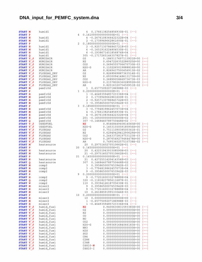
DNA_input_for_PEMFC_system.dna 3/4

START M humid1 4 0.1766138254856930E−01 ~~START P 4 0.1410000000000000E+01 ~~START H humid1 4 −0.2676108366422322E+04 ~~START M humid1 2 −0.1739949662861600E−01 ~~START P 2 0.1800000000000000E+01 ~~START H humid1 2 −0.9257130786845721E+03 ~~START M humid1 6 −0.1651916224804530E−01 ~~START H humid1 6 −0.1938671451856874E+04 ~~START Q humid1 305 −0.1717265146357827E−01 ~~START Y_J HUMIDAIR O2 0.1865117697113921E+00 ~~START Y_J HUMIDAIR N2 0.6947226352286025E+00 ~~START Y_J HUMIDAIR CO2 0.2696555706670730E−03 ~~START Y_J HUMIDAIR H2O−G 0.1102265019888816E+00 ~~START Y_J HUMIDAIR AR 0.8269437500456913E−02 ~~START Y_J FLUEGAS_DRY O2 0.8268969887363514E−01 ~~START Y_J FLUEGAS_DRY N2 0.6930094148613173E+00 ~~START Y_J FLUEGAS_DRY CO2 0.2689905866973673E−03 ~~START Y_J FLUEGAS_DRY H2O−G 0.2157802636028992E+00 ~~START Y_J FLUEGAS_DRY AR 0.8251632075450951E−02 ~~START M pemfc0d 1 0.6577509207186988E−03 ~~START P 1 0.2000000000000000E+01 ~~START H pemfc0d 1 −0.4649359485723336E+04 ~~START M pemfc0d 2 0.1739949662861600E−01 ~~START H pemfc0d 2 −0.9257130786845722E+03 ~~START M pemfc0d 3 −0.3958650007653942E−03 ~~START P 3 0.1858000000000000E+01 ~~START H pemfc0d 3 −0.7794819862457073E+04 ~~START M pemfc0d 4 −0.1766138254856930E−01 ~~START H pemfc0d 4 −0.2676108366422322E+04 ~~START E pemfc0d 201 −0.1650000000000000E+02 ~~START Q pemfc0d 307 −0.1468440789750448E+02 ~~START Y_J USEDFUEL H2 0.8546844940814045E+00 ~~START Y_J USEDFUEL H2O−G 0.1453155059185956E+00 ~~START Y_J FLUEGAS O2 0.7511109038500341E−01 ~~START Y_J FLUEGAS N2 0.6294942841290629E+00 ~~START Y_J FLUEGAS CO2 0.2443372819753123E−03 ~~START Y_J FLUEGAS H2O−G 0.2876549279464478E+00 ~~START Y_J FLUEGAS AR 0.7495360257510738E−02 ~~START M heatsource 20 0.2975140270510662E+01 ~~START P 20 0.1450000000000000E+01 ~~START H heatsource 20 0.4223194393308590E+03 ~~START M heatsource 21 −0.2975140270510662E+01 ~~START P 21 0.1450000000000000E+01 ~~START H heatsource 21 0.4272551420414354E+03 ~~START Q heatsource 307 0.1468440789750448E+02 ~~START M comp2 3 0.3958650007653942E−03 ~~START H comp2 3 −0.7794819862457073E+04 ~~START M comp2 9 −0.3958650007653942E−03 ~~START P 9 0.2000000000000000E+01 ~~START H comp2 9 −0.7725160033278889E+04 ~~START Q comp2 320 −0.1181823785611687E−01 ~~START W comp2 110 0.3939412618705630E−01 ~~START M mixer2 9 0.3958650007653942E−03 ~~START H mixer2 9 −0.7725160033278889E+04 ~~START M mixer2 10 0.2618859199533046E−03 ~~START P 10 0.2000000000000000E+01 ~~START H mixer2 10 0.0000000000000000E+00 ~~START M mixer2 1 −0.6577509207186988E−03 ~~START H mixer2 1 −0.4649359485723336E+04 ~~START Y_J humid_fuel H2 0.9400630831593383E+00 ~~START Y_J humid_fuel O2 0.0000000000000000E+00 ~~START Y_J humid_fuel N2 0.0000000000000000E+00 ~~START Y_J humid_fuel CO 0.0000000000000000E+00 ~~START Y_J humid_fuel NO 0.0000000000000000E+00 ~~START Y_J humid_fuel CO2 0.0000000000000000E+00 ~~START Y_J humid_fuel H2O−G 0.5993691684066183E−01 ~~START Y_J humid_fuel NH3 0.0000000000000000E+00 ~~START Y_J humid_fuel H2S 0.0000000000000000E+00 ~~START Y_J humid_fuel SO2 0.0000000000000000E+00 ~~START Y_J humid_fuel CH4 0.0000000000000000E+00 ~~START Y_J humid_fuel C2H6 0.0000000000000000E+00 ~~START Y_J humid_fuel C3H8 0.0000000000000000E+00 ~~START Y_J humid_fuel C4H10−N 0.0000000000000000E+00 ~~START Y_J humid_fuel C4H10−I 0.0000000000000000E+00 ~~

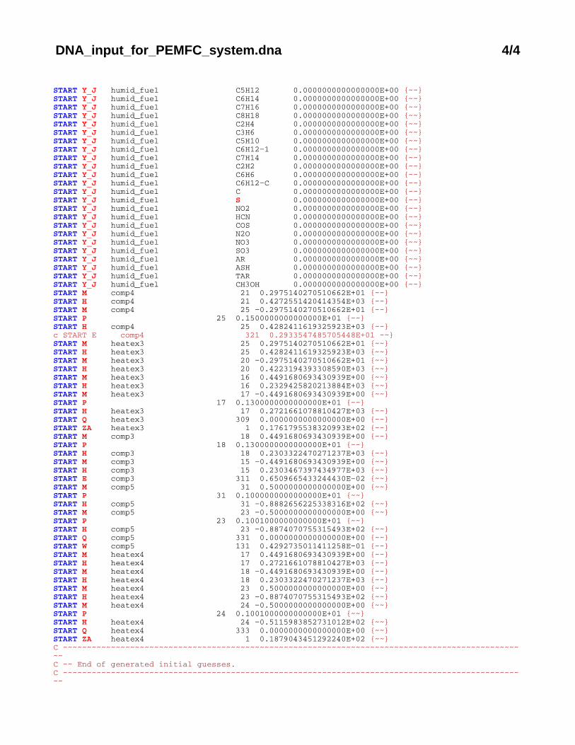
DNA_input_for_PEMFC_system.dna 4/4

START Y_J humid_fuel C5H12 0.0000000000000000E+00 ~~START Y_J humid_fuel C6H14 0.0000000000000000E+00 ~~START Y_J humid_fuel C7H16 0.0000000000000000E+00 ~~START Y_J humid_fuel C8H18 0.0000000000000000E+00 ~~START Y_J humid_fuel C2H4 0.0000000000000000E+00 ~~START Y_J humid_fuel C3H6 0.0000000000000000E+00 ~~START Y_J humid_fuel C5H10 0.0000000000000000E+00 ~~START Y_J humid_fuel C6H12−1 0.0000000000000000E+00 ~~START Y_J humid_fuel C7H14 0.0000000000000000E+00 ~~START Y_J humid_fuel C2H2 0.0000000000000000E+00 ~~START Y_J humid_fuel C6H6 0.0000000000000000E+00 ~~START Y_J humid_fuel C6H12−C 0.0000000000000000E+00 ~~START Y_J humid_fuel C 0.0000000000000000E+00 ~~START Y_J humid_fuel S 0.0000000000000000E+00 ~~START Y_J humid_fuel NO2 0.0000000000000000E+00 ~~START Y_J humid_fuel HCN 0.0000000000000000E+00 ~~START Y_J humid_fuel COS 0.0000000000000000E+00 ~~START Y_J humid_fuel N2O 0.0000000000000000E+00 ~~START Y_J humid_fuel NO3 0.0000000000000000E+00 ~~START Y_J humid_fuel SO3 0.0000000000000000E+00 ~~START Y_J humid_fuel AR 0.0000000000000000E+00 ~~START Y_J humid_fuel ASH 0.0000000000000000E+00 ~~START Y_J humid_fuel TAR 0.0000000000000000E+00 ~~START Y_J humid_fuel CH3OH 0.0000000000000000E+00 ~~START M comp4 21 0.2975140270510662E+01 ~~START H comp4 21 0.4272551420414354E+03 ~~START M comp4 25 −0.2975140270510662E+01 ~~START P 25 0.1500000000000000E+01 ~~START H comp4 25 0.4282411619325923E+03 ~~c START E comp4 321 0.2933547485705448E+01 ~~START M heatex3 25 0.2975140270510662E+01 ~~START H heatex3 25 0.4282411619325923E+03 ~~START M heatex3 20 −0.2975140270510662E+01 ~~START H heatex3 20 0.4223194393308590E+03 ~~START M heatex3 16 0.4491680693430939E+00 ~~START H heatex3 16 0.2329425820213884E+03 ~~START M heatex3 17 −0.4491680693430939E+00 ~~START P 17 0.1300000000000000E+01 ~~START H heatex3 17 0.2721661078810427E+03 ~~START Q heatex3 309 0.0000000000000000E+00 ~~START ZA heatex3 1 0.1761795538320993E+02 ~~START M comp3 18 0.4491680693430939E+00 ~~START P 18 0.1300000000000000E+01 ~~START H comp3 18 0.2303322470271237E+03 ~~START M comp3 15 −0.4491680693430939E+00 ~~START H comp3 15 0.2303467397434977E+03 ~~START E comp3 311 0.6509665433244430E−02 ~~START M comp5 31 0.5000000000000000E+00 ~~START P 31 0.1000000000000000E+01 ~~START H comp5 31 −0.8882656225338316E+02 ~~START M comp5 23 −0.5000000000000000E+00 ~~START P 23 0.1001000000000000E+01 ~~START H comp5 23 −0.8874070755315493E+02 ~~START Q comp5 331 0.0000000000000000E+00 ~~START W comp5 131 0.4292735011411258E−01 ~~START M heatex4 17 0.4491680693430939E+00 ~~START H heatex4 17 0.2721661078810427E+03 ~~START M heatex4 18 −0.4491680693430939E+00 ~~START H heatex4 18 0.2303322470271237E+03 ~~START M heatex4 23 0.5000000000000000E+00 ~~START H heatex4 23 −0.8874070755315493E+02 ~~START M heatex4 24 −0.5000000000000000E+00 ~~START P 24 0.1001000000000000E+01 ~~START H heatex4 24 −0.5115983852731012E+02 ~~START Q heatex4 333 0.0000000000000000E+00 ~~START ZA heatex4 1 0.1879043451292240E+02 ~~C ~~~~~~~~~~~~~~~~~~~~~~~~~~~~~~~~~~~~~~~~~~~~~~~~~~~~~~~~~~~~~~~~~~~~~~~~~~~~~~~~~~~~~~~~~~~~~~~~~C ~~ End of generated initial guesses.C ~~~~~~~~~~~~~~~~~~~~~~~~~~~~~~~~~~~~~~~~~~~~~~~~~~~~~~~~~~~~~~~~~~~~~~~~~~~~~~~~~~~~~~~~~~~~~~~~~

A.7 DNA Output for PEMFC system

148

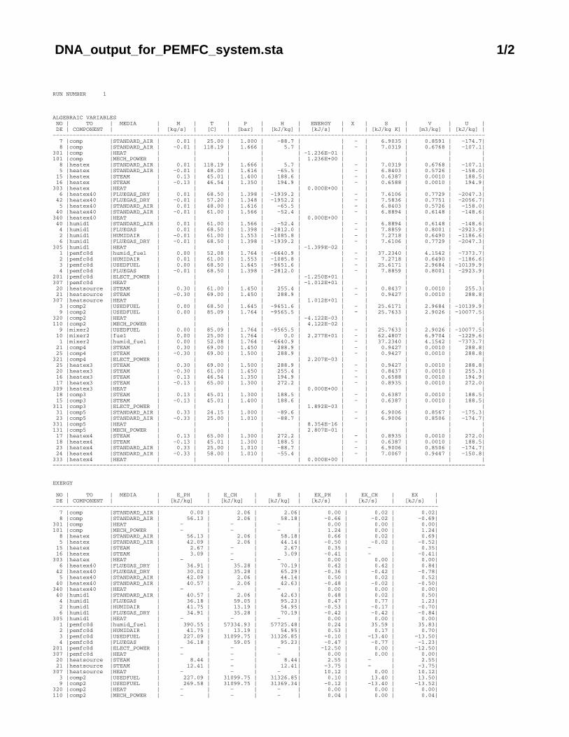
DNA_output_for_PEMFC_system.sta 1/2

RUN NUMBER 1

ALGEBRAIC VARIABLES NO | TO | MEDIA | M | T | P | H | ENERGY | X | S | V | U | DE | COMPONENT | | [kg/s] | [C] | [bar] | [kJ/kg] | [kJ/s] | | [kJ/kg K] | [m3/kg] | [kJ/kg] |−−−−−−−−−−−−−−−−−−−−−−−−−−−−−−−−−−−−−−−−−−−−−−−−−−−−−−−−−−−−−−−−−−−−−−−−−−−−−−−−−−−−−−−−−−−−−−−−−−−−−−−−−−−−−−−−−−−−−−−−−−−−−−−−− 7 |comp |STANDARD_AIR | 0.01 | 25.00 | 1.000 | −88.7 | | − | 6.9035 | 0.8591 | −174.7| 8 |comp |STANDARD_AIR | −0.01 | 118.19 | 1.666 | 5.7 | | − | 7.0319 | 0.6768 | −107.1| 301 |comp |HEAT | | | | | −1.236E−01 | | | | |101 |comp |MECH_POWER | | | | | 1.236E+00 | | | | | 8 |heatex |STANDARD_AIR | 0.01 | 118.19 | 1.666 | 5.7 | | − | 7.0319 | 0.6768 | −107.1| 5 |heatex |STANDARD_AIR | −0.01 | 48.00 | 1.616 | −65.5 | | − | 6.8403 | 0.5726 | −158.0| 15 |heatex |STEAM | 0.13 | 45.01 | 1.400 | 188.6 | | − | 0.6387 | 0.0010 | 188.5| 16 |heatex |STEAM | −0.13 | 46.54 | 1.350 | 194.9 | | − | 0.6588 | 0.0010 | 194.9| 303 |heatex |HEAT | | | | | 0.000E+00 | | | | | 6 |heatex40 |FLUEGAS_DRY | 0.01 | 68.50 | 1.398 | −1939.2 | | − | 7.6106 | 0.7729 | −2047.3| 42 |heatex40 |FLUEGAS_DRY | −0.01 | 57.20 | 1.348 | −1952.2 | | − | 7.5836 | 0.7751 | −2056.7| 5 |heatex40 |STANDARD_AIR | 0.01 | 48.00 | 1.616 | −65.5 | | − | 6.8403 | 0.5726 | −158.0| 40 |heatex40 |STANDARD_AIR | −0.01 | 61.00 | 1.566 | −52.4 | | − | 6.8894 | 0.6148 | −148.6| 340 |heatex40 |HEAT | | | | | 0.000E+00 | | | | | 40 |humid1 |STANDARD_AIR | 0.01 | 61.00 | 1.566 | −52.4 | | − | 6.8894 | 0.6148 | −148.6| 4 |humid1 |FLUEGAS | 0.01 | 68.50 | 1.398 | −2812.0 | | − | 7.8859 | 0.8001 | −2923.9| 2 |humid1 |HUMIDAIR | −0.01 | 61.00 | 1.553 | −1085.8 | | − | 7.2718 | 0.6490 | −1186.6| 6 |humid1 |FLUEGAS_DRY | −0.01 | 68.50 | 1.398 | −1939.2 | | − | 7.6106 | 0.7729 | −2047.3| 305 |humid1 |HEAT | | | | | −1.399E−02 | | | | | 1 |pemfc0d |humid_fuel | 0.00 | 52.08 | 1.764 | −6640.9 | | − | 37.2340 | 4.1542 | −7373.7| 2 |pemfc0d |HUMIDAIR | 0.01 | 61.00 | 1.553 | −1085.8 | | − | 7.2718 | 0.6490 | −1186.6| 3 |pemfc0d |USEDFUEL | 0.00 | 68.50 | 1.645 | −9651.6 | | − | 25.6171 | 2.9684 | −10139.9| 4 |pemfc0d |FLUEGAS | −0.01 | 68.50 | 1.398 | −2812.0 | | − | 7.8859 | 0.8001 | −2923.9| 201 |pemfc0d |ELECT_POWER | | | | | −1.250E+01 | | | | |307 |pemfc0d |HEAT | | | | | −1.012E+01 | | | | | 20 |heatsource |STEAM | 0.30 | 61.00 | 1.450 | 255.4 | | − | 0.8437 | 0.0010 | 255.3| 21 |heatsource |STEAM | −0.30 | 69.00 | 1.450 | 288.9 | | − | 0.9427 | 0.0010 | 288.8| 307 |heatsource |HEAT | | | | | 1.012E+01 | | | | | 3 |comp2 |USEDFUEL | 0.00 | 68.50 | 1.645 | −9651.6 | | − | 25.6171 | 2.9684 | −10139.9| 9 |comp2 |USEDFUEL | 0.00 | 85.09 | 1.764 | −9565.5 | | − | 25.7633 | 2.9026 | −10077.5| 320 |comp2 |HEAT | | | | | −4.122E−03 | | | | |110 |comp2 |MECH_POWER | | | | | 4.122E−02 | | | | | 9 |mixer2 |USEDFUEL | 0.00 | 85.09 | 1.764 | −9565.5 | | − | 25.7633 | 2.9026 | −10077.5| 10 |mixer2 |fuel | 0.00 | 25.00 | 1.764 | 0.0 | 2.277E+01 | − | 62.4807 | 6.9704 | −1229.6| 1 |mixer2 |humid_fuel | 0.00 | 52.08 | 1.764 | −6640.9 | | − | 37.2340 | 4.1542 | −7373.7| 21 |comp4 |STEAM | 0.30 | 69.00 | 1.450 | 288.9 | | − | 0.9427 | 0.0010 | 288.8| 25 |comp4 |STEAM | −0.30 | 69.00 | 1.500 | 288.9 | | − | 0.9427 | 0.0010 | 288.8| 321 |comp4 |ELECT_POWER | | | | | 2.207E−03 | | | | | 25 |heatex3 |STEAM | 0.30 | 69.00 | 1.500 | 288.9 | | − | 0.9427 | 0.0010 | 288.8| 20 |heatex3 |STEAM | −0.30 | 61.00 | 1.450 | 255.4 | | − | 0.8437 | 0.0010 | 255.3| 16 |heatex3 |STEAM | 0.13 | 46.54 | 1.350 | 194.9 | | − | 0.6588 | 0.0010 | 194.9| 17 |heatex3 |STEAM | −0.13 | 65.00 | 1.300 | 272.2 | | − | 0.8935 | 0.0010 | 272.0| 309 |heatex3 |HEAT | | | | | 0.000E+00 | | | | | 18 |comp3 |STEAM | 0.13 | 45.01 | 1.300 | 188.5 | | − | 0.6387 | 0.0010 | 188.5| 15 |comp3 |STEAM | −0.13 | 45.01 | 1.400 | 188.6 | | − | 0.6387 | 0.0010 | 188.5| 311 |comp3 |ELECT_POWER | | | | | 1.892E−03 | | | | | 31 |comp5 |STANDARD_AIR | 0.33 | 24.15 | 1.000 | −89.6 | | − | 6.9006 | 0.8567 | −175.3| 23 |comp5 |STANDARD_AIR | −0.33 | 25.00 | 1.010 | −88.7 | | − | 6.9006 | 0.8506 | −174.7| 331 |comp5 |HEAT | | | | | 8.354E−16 | | | | |131 |comp5 |MECH_POWER | | | | | 2.807E−01 | | | | | 17 |heatex4 |STEAM | 0.13 | 65.00 | 1.300 | 272.2 | | − | 0.8935 | 0.0010 | 272.0| 18 |heatex4 |STEAM | −0.13 | 45.01 | 1.300 | 188.5 | | − | 0.6387 | 0.0010 | 188.5| 23 |heatex4 |STANDARD_AIR | 0.33 | 25.00 | 1.010 | −88.7 | | − | 6.9006 | 0.8506 | −174.7| 24 |heatex4 |STANDARD_AIR | −0.33 | 58.00 | 1.010 | −55.4 | | − | 7.0067 | 0.9447 | −150.8| 333 |heatex4 |HEAT | | | | | 0.000E+00 | | | | |−−−−−−−−−−−−−−−−−−−−−−−−−−−−−−−−−−−−−−−−−−−−−−−−−−−−−−−−−−−−−−−−−−−−−−−−−−−−−−−−−−−−−−−−−−−−−−−−−−−−−−−−−−−−−−−−−−−−−−−−−−−−−−−−−

EXERGY

NO | TO | MEDIA | E_PH | E_CH | E | EX_PH | EX_CH | EX | DE | COMPONENT | | [kJ/kg] | [kJ/kg] | [kJ/kg] | [kJ/s] | [kJ/s] | [kJ/s] |−−−−−−−−−−−−−−−−−−−−−−−−−−−−−−−−−−−−−−−−−−−−−−−−−−−−−−−−−−−−−−−−−−−−−−−−−−−−−−−−−−−−−−−−−−−−−−−−−−−−−−−−−−−−−−−−−−− 7 |comp |STANDARD_AIR | 0.00 | 2.06 | 2.06| 0.00 | 0.02 | 0.02| 8 |comp |STANDARD_AIR | 56.13 | 2.06 | 58.18| −0.66 | −0.02 | −0.69| 301 |comp |HEAT | − | − | − | 0.00 | 0.00 | 0.00| 101 |comp |MECH_POWER | − | − | − | 1.24 | 0.00 | 1.24| 8 |heatex |STANDARD_AIR | 56.13 | 2.06 | 58.18| 0.66 | 0.02 | 0.69| 5 |heatex |STANDARD_AIR | 42.09 | 2.06 | 44.14| −0.50 | −0.02 | −0.52| 15 |heatex |STEAM | 2.67 | − | 2.67| 0.35 | − | 0.35| 16 |heatex |STEAM | 3.09 | − | 3.09| −0.41 | − | −0.41| 303 |heatex |HEAT | − | − | − | 0.00 | 0.00 | 0.00| 6 |heatex40 |FLUEGAS_DRY | 34.91 | 35.28 | 70.19| 0.42 | 0.42 | 0.84| 42 |heatex40 |FLUEGAS_DRY | 30.02 | 35.28 | 65.29| −0.36 | −0.42 | −0.78| 5 |heatex40 |STANDARD_AIR | 42.09 | 2.06 | 44.14| 0.50 | 0.02 | 0.52| 40 |heatex40 |STANDARD_AIR | 40.57 | 2.06 | 42.63| −0.48 | −0.02 | −0.50| 340 |heatex40 |HEAT | − | − | − | 0.00 | 0.00 | 0.00| 40 |humid1 |STANDARD_AIR | 40.57 | 2.06 | 42.63| 0.48 | 0.02 | 0.50| 4 |humid1 |FLUEGAS | 36.18 | 59.05 | 95.23| 0.47 | 0.77 | 1.23| 2 |humid1 |HUMIDAIR | 41.75 | 13.19 | 54.95| −0.53 | −0.17 | −0.70| 6 |humid1 |FLUEGAS_DRY | 34.91 | 35.28 | 70.19| −0.42 | −0.42 | −0.84| 305 |humid1 |HEAT | − | − | − | 0.00 | 0.00 | 0.00| 1 |pemfc0d |humid_fuel | 390.55 | 57334.93 | 57725.48| 0.24 | 35.59 | 35.83| 2 |pemfc0d |HUMIDAIR | 41.75 | 13.19 | 54.95| 0.53 | 0.17 | 0.70| 3 |pemfc0d |USEDFUEL | 227.09 | 31099.75 | 31326.85| −0.10 | −13.40 | −13.50| 4 |pemfc0d |FLUEGAS | 36.18 | 59.05 | 95.23| −0.47 | −0.77 | −1.23| 201 |pemfc0d |ELECT_POWER | − | − | − | −12.50 | 0.00 | −12.50| 307 |pemfc0d |HEAT | − | − | − | 0.00 | 0.00 | 0.00| 20 |heatsource |STEAM | 8.44 | − | 8.44| 2.55 | − | 2.55| 21 |heatsource |STEAM | 12.41 | − | 12.41| −3.75 | − | −3.75| 307 |heatsource |HEAT | − | − | − | 10.12 | 0.00 | 10.12| 3 |comp2 |USEDFUEL | 227.09 | 31099.75 | 31326.85| 0.10 | 13.40 | 13.50| 9 |comp2 |USEDFUEL | 269.58 | 31099.75 | 31369.34| −0.12 | −13.40 | −13.52| 320 |comp2 |HEAT | − | − | − | 0.00 | 0.00 | 0.00| 110 |comp2 |MECH_POWER | − | − | − | 0.04 | 0.00 | 0.04|

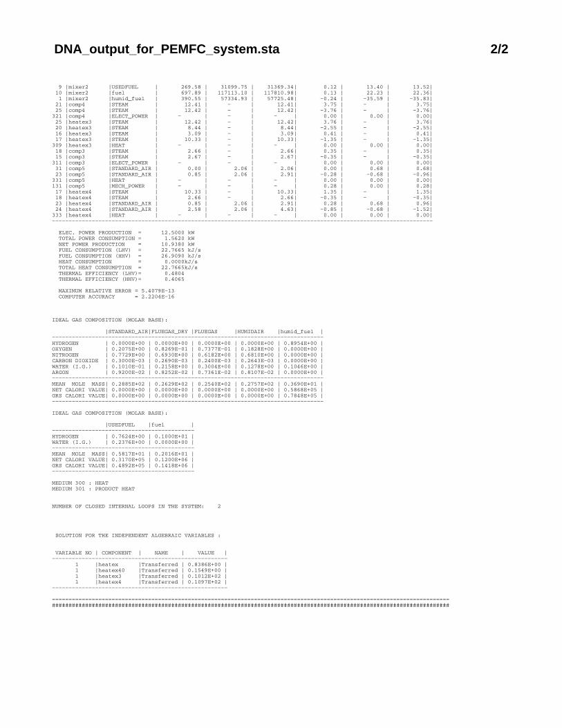
DNA_output_for_PEMFC_system.sta 2/2

9 |mixer2 |USEDFUEL | 269.58 | 31099.75 | 31369.34| 0.12 | 13.40 | 13.52| 10 |mixer2 |fuel | 697.89 | 117113.10 | 117810.98| 0.13 | 22.23 | 22.36| 1 |mixer2 |humid_fuel | 390.55 | 57334.93 | 57725.48| −0.24 | −35.59 | −35.83| 21 |comp4 |STEAM | 12.41 | − | 12.41| 3.75 | − | 3.75| 25 |comp4 |STEAM | 12.42 | − | 12.42| −3.76 | − | −3.76| 321 |comp4 |ELECT_POWER | − | − | − | 0.00 | 0.00 | 0.00| 25 |heatex3 |STEAM | 12.42 | − | 12.42| 3.76 | − | 3.76| 20 |heatex3 |STEAM | 8.44 | − | 8.44| −2.55 | − | −2.55| 16 |heatex3 |STEAM | 3.09 | − | 3.09| 0.41 | − | 0.41| 17 |heatex3 |STEAM | 10.33 | − | 10.33| −1.35 | − | −1.35| 309 |heatex3 |HEAT | − | − | − | 0.00 | 0.00 | 0.00| 18 |comp3 |STEAM | 2.66 | − | 2.66| 0.35 | − | 0.35| 15 |comp3 |STEAM | 2.67 | − | 2.67| −0.35 | − | −0.35| 311 |comp3 |ELECT_POWER | − | − | − | 0.00 | 0.00 | 0.00| 31 |comp5 |STANDARD_AIR | 0.00 | 2.06 | 2.06| 0.00 | 0.68 | 0.68| 23 |comp5 |STANDARD_AIR | 0.85 | 2.06 | 2.91| −0.28 | −0.68 | −0.96| 331 |comp5 |HEAT | − | − | − | 0.00 | 0.00 | 0.00| 131 |comp5 |MECH_POWER | − | − | − | 0.28 | 0.00 | 0.28| 17 |heatex4 |STEAM | 10.33 | − | 10.33| 1.35 | − | 1.35| 18 |heatex4 |STEAM | 2.66 | − | 2.66| −0.35 | − | −0.35| 23 |heatex4 |STANDARD_AIR | 0.85 | 2.06 | 2.91| 0.28 | 0.68 | 0.96| 24 |heatex4 |STANDARD_AIR | 2.58 | 2.06 | 4.63| −0.85 | −0.68 | −1.52| 333 |heatex4 |HEAT | − | − | − | 0.00 | 0.00 | 0.00| −−−−−−−−−−−−−−−−−−−−−−−−−−−−−−−−−−−−−−−−−−−−−−−−−−−−−−−−−−−−−−−−−−−−−−−−−−−−−−−−−−−−−−−−−−−−−−−−−−−−−−−−−−−−−−−−−−− ELEC. POWER PRODUCTION = 12.5000 kW TOTAL POWER CONSUMPTION = 1.5620 kW NET POWER PRODUCTION = 10.9380 kW FUEL CONSUMPTION (LHV) = 22.7665 kJ/s FUEL CONSUMPTION (HHV) = 26.9090 kJ/s HEAT CONSUMPTION = 0.0000kJ/s TOTAL HEAT CONSUMPTION = 22.7665kJ/s THERMAL EFFICIENCY (LHV)= 0.4804 THERMAL EFFICIENCY (HHV)= 0.4065 MAXIMUM RELATIVE ERROR = 5.4079E−13 COMPUTER ACCURACY = 2.2204E−16 IDEAL GAS COMPOSITION (MOLAR BASE): |STANDARD_AIR|FLUEGAS_DRY |FLUEGAS |HUMIDAIR |humid_fuel |−−−−−−−−−−−−−−−−−−−−−−−−−−−−−−−−−−−−−−−−−−−−−−−−−−−−−−−−−−−−−−−−−−−−−−−−−−−−−−−−−−HYDROGEN | 0.0000E+00 | 0.0000E+00 | 0.0000E+00 | 0.0000E+00 | 0.8954E+00 | OXYGEN | 0.2075E+00 | 0.8269E−01 | 0.7377E−01 | 0.1828E+00 | 0.0000E+00 | NITROGEN | 0.7729E+00 | 0.6930E+00 | 0.6182E+00 | 0.6810E+00 | 0.0000E+00 | CARBON DIOXIDE | 0.3000E−03 | 0.2690E−03 | 0.2400E−03 | 0.2643E−03 | 0.0000E+00 | WATER (I.G.) | 0.1010E−01 | 0.2158E+00 | 0.3004E+00 | 0.1278E+00 | 0.1046E+00 | ARGON | 0.9200E−02 | 0.8252E−02 | 0.7361E−02 | 0.8107E−02 | 0.0000E+00 | −−−−−−−−−−−−−−−−−−−−−−−−−−−−−−−−−−−−−−−−−−−−−−−−−−−−−−−−−−−−−−−−−−−−−−−−−−−−−−−−−−MEAN MOLE MASS| 0.2885E+02 | 0.2629E+02 | 0.2540E+02 | 0.2757E+02 | 0.3690E+01 | NET CALORI VALUE| 0.0000E+00 | 0.0000E+00 | 0.0000E+00 | 0.0000E+00 | 0.5868E+05 | GRS CALORI VALUE| 0.0000E+00 | 0.0000E+00 | 0.0000E+00 | 0.0000E+00 | 0.7848E+05 | −−−−−−−−−−−−−−−−−−−−−−−−−−−−−−−−−−−−−−−−−−−−−−−−−−−−−−−−−−−−−−−−−−−−−−−−−−−−−−−−−− IDEAL GAS COMPOSITION (MOLAR BASE): |USEDFUEL |fuel |−−−−−−−−−−−−−−−−−−−−−−−−−−−−−−−−−−−−−−−−−−−HYDROGEN | 0.7624E+00 | 0.1000E+01 | WATER (I.G.) | 0.2376E+00 | 0.0000E+00 | −−−−−−−−−−−−−−−−−−−−−−−−−−−−−−−−−−−−−−−−−−−MEAN MOLE MASS| 0.5817E+01 | 0.2016E+01 | NET CALORI VALUE| 0.3170E+05 | 0.1200E+06 | GRS CALORI VALUE| 0.4892E+05 | 0.1418E+06 | −−−−−−−−−−−−−−−−−−−−−−−−−−−−−−−−−−−−−−−−−−− MEDIUM 300 : HEATMEDIUM 301 : PRODUCT HEAT NUMBER OF CLOSED INTERNAL LOOPS IN THE SYSTEM: 2 SOLUTION FOR THE INDEPENDENT ALGEBRAIC VARIABLES : VARIABLE NO | COMPONENT | NAME | VALUE |−−−−−−−−−−−−−−−−−−−−−−−−−−−−−−−−−−−−−−−−−−−−−−−−−−−−− 1 |heatex |Transferred | 0.8386E+00 | 1 |heatex40 |Transferred | 0.1549E+00 | 1 |heatex3 |Transferred | 0.1012E+02 | 1 |heatex4 |Transferred | 0.1097E+02 |−−−−−−−−−−−−−−−−−−−−−−−−−−−−−−−−−−−−−−−−−−−−−−−−−−−−− ========================================================================================================================########################################################################################################################

Appendix B

Paper I

Development and validation of a simple analytical model of the Proton Exchange Mem-brane Fuel Cell (PEMFC) in a fork-lift truck power system

151

This article was downloaded by: [DTU Library]On: 28 April 2013, At: 13:32Publisher: Taylor & FrancisInforma Ltd Registered in England and Wales Registered Number: 1072954 Registeredoffice: Mortimer House, 37-41 Mortimer Street, London W1T 3JH, UK

International Journal of Green EnergyPublication details, including instructions for authors andsubscription information:http://www.tandfonline.com/loi/ljge20

Development and Validation of a SimpleAnalytical Model of the Proton ExchangeMembrane Fuel Cell (PEMFC) in a Fork-Lift Truck Power SystemElham Hosseinzadeh a & Masoud Rokni aa Thermal Energy Section, Department of Mechanical Engineering,Technical University of Denmark (DTU), Lyngby, DenmarkAccepted author version posted online: 14 May 2012.Version ofrecord first published: 26 Mar 2013.

To cite this article: Elham Hosseinzadeh & Masoud Rokni (2013): Development and Validation of aSimple Analytical Model of the Proton Exchange Membrane Fuel Cell (PEMFC) in a Fork-Lift TruckPower System, International Journal of Green Energy, 10:5, 523-543

To link to this article: http://dx.doi.org/10.1080/15435075.2012.678525

PLEASE SCROLL DOWN FOR ARTICLE

Full terms and conditions of use: http://www.tandfonline.com/page/terms-and-conditions

This article may be used for research, teaching, and private study purposes. Anysubstantial or systematic reproduction, redistribution, reselling, loan, sub-licensing,systematic supply, or distribution in any form to anyone is expressly forbidden.

The publisher does not give any warranty express or implied or make any representationthat the contents will be complete or accurate or up to date. The accuracy of anyinstructions, formulae, and drug doses should be independently verified with primarysources. The publisher shall not be liable for any loss, actions, claims, proceedings,demand, or costs or damages whatsoever or howsoever caused arising directly orindirectly in connection with or arising out of the use of this material.

International Journal of Green Energy, 10: 523–543, 2013Copyright © Taylor & Francis Group, LLCISSN: 1543-5075 print / 1543-5083 onlineDOI: 10.1080/15435075.2012.678525

DEVELOPMENT AND VALIDATION OF A SIMPLEANALYTICAL MODEL OF THE PROTON EXCHANGEMEMBRANE FUEL CELL (PEMFC) IN A FORK-LIFTTRUCK POWER SYSTEM

Elham Hosseinzadeh and Masoud RokniThermal Energy Section, Department of Mechanical Engineering, TechnicalUniversity of Denmark (DTU), Lyngby, Denmark

In this study, a general proton exchange membrane fuel cell (PEMFC) model has beendeveloped in order to investigate the balance of plant of a fork-lift truck thermodynami-cally. The model takes into account the effects of pressure losses, water crossovers, humidityaspects, and voltage overpotentials in the cells. Moreover, it is zero-dimensional and isassumed to be steady state. The system includes a compressor, an air humidifier, a set ofheat exchangers, and a stack that together build up the anode circuit, the cathode circuit,and the cooling loop. Several issues are discussed: water management, system sensitivity tocoolant inlet temperature, air and fuel stoichiometry, anode inlet pressure, stack operatingconditions, etc. System efficiency and electrical power at different operating conditions arealso discussed. The results show that 12–30% of stack power is allocated for the auxilarycomponents depending on the stack power or current. Further, at the higher current den-sities, heat losses and net power of the system increase, while system efficiency decreases.Furthermore, the system performance was not sensitive to the coolant temperature whenwater is used as the coolant.

Keywords: PEMFC; Fuel cell; System layout; Fork-lift; General model; Polarizationcurve

INTRODUCTION

Fuel cells have received more attention during the past decade and appear to havethe potential to become the power source of future. The main reason is the negative con-sequences of using fossil fuels in power generation. The first problem with fossil fuels isthat they are a finite source of energy and sooner or later will be exhausted. The secondproblem is that they are not environmental friendly: global warming and climate changesnow seen to be the consequences of fossil fuel emissions. Fossil fuels are extensively usedin the automobile industry and are the most significant source of greenhouse gas emissions.Finding an alternative energy source to fossil fuels is therefore inevitable in the automo-bile industry, which guides the development of next generation vehicles. Among varioustypes of fuel cells, proton exchange membrane (PEM) fuel cells (PEMFC) are seen by theautomotive industry as being the most promising.

Address correspondence to Elham Hosseinzadeh, Thermal Energy Section, Department of MechanicalEngineering, Technical University of Denmark (DTU), Building 403, Room 111 2800 Kgs, Lyngby, Denmark.E-mail: ehos@mek.dtu.dk

523

Dow

nloa

ded

by [

DT

U L

ibra

ry]

at 1

3:32

28

Apr

il 20

13

524 HOSSEINZADEH AND ROKNI

PEM fuel cells in particular have desirable properties, such as a low operating tem-perature, which provide the possibility of using cheaper components. However, lack of ahydrogen infrastructure is considered the biggest obstacle to the introduction of fuel cellvehicles. Due to its low temperature operation there, no internal reforming can take placeand only pure hydrogen can be used as a fuel, which is expensive. In order for PEM fuelcell systems to be competitive with internal combustion engines, they must function as wellas conventional internal combustion engines (ICE). Fuel cells offer several advantages overeither ICE generators (noise, expected higher reliability, and lower maintenance) or batter-ies (weight, lifetime, maintenance). But today, PEM fuel cell automotive systems are tooexpensive for widespread marketing. These systems still need some improvement so thatthey can compete with ICE. A fuel cell stack is obviously the heart of a fuel cell system;however, without the supporting equipment the stack itself would not be very useful. Thefuel cell system typically involves the following accessory subsystems: Oxidant supply (pure oxygen or air) Fuel supply (pure hydrogen or hydrogen-rich gas) Heat management Water management Power conditioning Instrumentation and control

There are two distinct approaches that may be taken when modeling the fuel cell sys-tems. The first is modeling the details of a single stack and using the operating conditionsto determine the current–voltage curve, and the second one is modeling the fuel cell sys-tem based on voltage–current output for an existing fuel cell stack and developing modelsfor auxiliary components. Very little attention has been paid to optimizing the entire plantsystem to make the fuel cell system work efficiently. In order to have a comprehensiveunderstanding of a fuel cell, one needs to look at its operation in the system with all nec-essary accessory components. Modeling a fuel cell stack alone does not serve the purpose.In order to investigate and optimize a fuel cell system, it is necessary to develop a compre-hensive model of the stack. There are many articles in the literature that have focused onnumerical modeling of the stack and the detailed phenomena that occur in the stack.

Following authors developed mathematical models based on analytical approaches.Yuan, Rokni, and Sunden (2003) developed a three-dimensional (3D) computational fluiddynamics (CFD) model of a PEM fuel cell by taking into account the electrochemical,mass, and heat transfer phenomena occurring in all of its regions simultaneously and alsothe effect of operating conditions, temperatures, and pressures on the stack efficiency.Matamoros and Bruggemann (2007) studied non-isothermal and 3D simulations to predictthe concentration and ohmic losses in a free-breathing PEMFC under diverse conditions.The results showed that humidification and oxygen transport phenomena were the mostlimiting factors to consider. Martins et al. (2009) reported a simplified and comprehen-sive model of PEMFC that takes into account the geometric design of the stack that wasvalidated against experimental data from 10 commercial stacks. Yu, Zhou, and Sobiesiak(2005) developed a water and thermal management model for one of the stacks of theBallard Company to investigate its performance. The stack power, heat, and water genera-tion as well as operating temperature were measured by their proposed model. Also, theirmodel could predict the dynamic performance of the stack temperature, the cell voltage,and the power as a function of time. Patel et al. (2008) carried out a 3D numerical study

Dow

nloa

ded

by [

DT

U L

ibra

ry]

at 1

3:32

28

Apr

il 20

13

MODEL OF THE PROTON EXCHANGE MEMBRANE FUEL CELL 525

to analyze flow, heat, and mass transfer as well as current distribution in a single half-cell cathode duct of a PEM fuel cell. Wang et al. (2011) reviewed the existing literatureconcerning flow mal-distributions in PEMFC stacks. Yuan and Sundén (2004) numericallyinvestigated and analyzed gas flow and heat transfer for both cathode and anode ducts ofPEM fuel cells.

Spinelli et al. (2008) and Haji (2011) provided a discussion of the polarization curvein PEMFC. Spinelli et al. (2008) applied a semi-empirical approach based on a simplifiedmathematical model to fit the experimental polarization data. The model could provide anestimation of hydrogen crossover and also possible change of ohmic resistance with currentdensity. Haji (2011) modeled the experimentally obtained I-V data of a 40 W fuel cellby estimating the parameters in the theoretical equation that describes the voltage outputversus the current. In some papers, key parameters estimation for the polarization curvewas proposed. Santarelli, Torchio, and Cochis (2006) briefly reviewed the main parameters(exchange current density, cell resistance, internal current density, and limiting currentdensity) and their study showed that three parameters of the cell polarization curve modelcan be simultaneously estimated: the cathode exchange current density, the cell resistance,and the internal current density.

Other papers have discussed electrolyte properties and water diffusion phenomena inthe stack. Yan et al. (2006) studied a transient analysis of water transport in a PEM fuel cellin theory. It was shown that in a thinner PEMFC, water was more uniformly distributed andalso that insufficient humidification led to relatively small water content in the membraneand increased the time for reaching a steady-state condition. Liu, Lu, and Wang (2006)reported experimental measurements of the net water transport coefficient distribution forthe first time. They showed that the local current density is dominated by the membranehydration and that the gas relative humidity has a large effect on the water transport throughthe membrane.

Many researchers have taken the second approach, incorporating PEM fuel cell I–Vcurves for existing fuel cells into a system model to examine fuel cell system performancein automotive applications. Incorporation of a fuel cell system model into a vehicle simu-lator makes it possible to assess fuel cell system performance in automotive applicationsunder typical driving conditions. A small number of papers have studied fuel cell systems.Ahluwalia and Wang (2005) provided an analysis of the design attributes and performanceof load-following fuel cell systems for hybrid vehicles with an energy storage device thatis operated in a charge-sustaining mode. Cordner et al. (2010) designed and built a 13 kWautomotive PEMFC system. Individual subsystems are designed, independently tested onthe bench, and then integrated into a complete balance of plant. In their paper, cell degra-dation mechanisms were investigated and were used to provide data for system controllerthat was built in LabVIEW program. Corbo, Migliardini, and Veneri (2007) designed alaboratory fuel cell system based on a 20 kW H2/air PEM stack and evaluated the effectof the main operative variables (temperature, pressure, and stoichiometric ratio) on stackpower and efficiency. Reactant feeding, humidification, and cooling problems were alsodiscussed.

To improve a complete fuel cell system, having a comprehensive model of the stackbesides auxiliary components is necessary. In the current study, more attempts have beenput to investigate the balance of plant that was not analytically discussed in many otherstudies. Firstly, a simple but general zero-dimensional and steady-state model for PEMFChas been developed. The presented polarization curve for the stack captures the experimen-tal data very well. This model can represent the behavior of various PEM stacks regardless

Dow

nloa

ded

by [

DT

U L

ibra

ry]

at 1

3:32

28

Apr

il 20

13

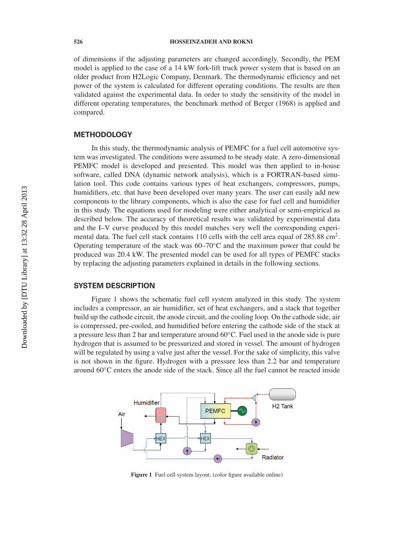
526 HOSSEINZADEH AND ROKNI

of dimensions if the adjusting parameters are changed accordingly. Secondly, the PEMmodel is applied to the case of a 14 kW fork-lift truck power system that is based on anolder product from H2Logic Company, Denmark. The thermodynamic efficiency and netpower of the system is calculated for different operating conditions. The results are thenvalidated against the experimental data. In order to study the sensitivity of the model indifferent operating temperatures, the benchmark method of Berger (1968) is applied andcompared.

METHODOLOGY

In this study, the thermodynamic analysis of PEMFC for a fuel cell automotive sys-tem was investigated. The conditions were assumed to be steady state. A zero-dimensionalPEMFC model is developed and presented. This model was then applied to in-housesoftware, called DNA (dynamic network analysis), which is a FORTRAN-based simu-lation tool. This code contains various types of heat exchangers, compressors, pumps,humidifiers, etc. that have been developed over many years. The user can easily add newcomponents to the library components, which is also the case for fuel cell and humidifierin this study. The equations used for modeling were either analytical or semi-empirical asdescribed below. The accuracy of theoretical results was validated by experimental dataand the I–V curve produced by this model matches very well the corresponding experi-mental data. The fuel cell stack contains 110 cells with the cell area equal of 285.88 cm2.Operating temperature of the stack was 60–70C and the maximum power that could beproduced was 20.4 kW. The presented model can be used for all types of PEMFC stacksby replacing the adjusting parameters explained in details in the following sections.

SYSTEM DESCRIPTION

Figure 1 shows the schematic fuel cell system analyzed in this study. The systemincludes a compressor, an air humidifier, set of heat exchangers, and a stack that togetherbuild up the cathode circuit, the anode circuit, and the cooling loop. On the cathode side, airis compressed, pre-cooled, and humidified before entering the cathode side of the stack ata pressure less than 2 bar and temperature around 60C. Fuel used in the anode side is purehydrogen that is assumed to be pressurized and stored in vessel. The amount of hydrogenwill be regulated by using a valve just after the vessel. For the sake of simplicity, this valveis not shown in the figure. Hydrogen with a pressure less than 2.2 bar and temperaturearound 60C enters the anode side of the stack. Since all the fuel cannot be reacted inside

Figure 1 Fuel cell system layout. (color figure available online)

Dow

nloa

ded

by [

DT

U L

ibra

ry]

at 1

3:32

28

Apr

il 20

13

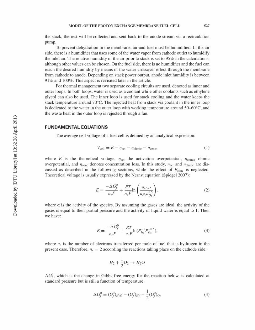
MODEL OF THE PROTON EXCHANGE MEMBRANE FUEL CELL 527

the stack, the rest will be collected and sent back to the anode stream via a recirculationpump.

To prevent dehydration in the membrane, air and fuel must be humidified. In the airside, there is a humidifier that uses some of the water vapor from cathode outlet to humidifythe inlet air. The relative humidity of the air prior to stack is set to 95% in the calculations,although other values can be chosen. On the fuel side, there is no humidifier and the fuel canreach the desired humidity by means of the water crossover effect through the membranefrom cathode to anode. Depending on stack power output, anode inlet humidity is between91% and 100%. This aspect is revisited later in the article.

For thermal management two separate cooling circuits are used, denoted as inner andouter loops. In both loops, water is used as a coolant while other coolants such as ethyleneglycol can also be used. The inner loop is used for stack cooling and the water keeps thestack temperature around 70C. The rejected heat from stack via coolant in the inner loopis dedicated to the water in the outer loop with working temperature around 50–60C, andthe waste heat in the outer loop is rejected through a fan.

FUNDAMENTAL EQUATIONS

The average cell voltage of a fuel cell is defined by an analytical expression:

Vcell = E − ηact − ηohmic − ηconc, (1)

where E is the theoretical voltage, ηact the activation overpotential, ηohmic ohmicoverpotential, and ηconc denotes concentration loss. In this study, ηact and ηohmic are dis-cussed as described in the following sections, while the effect of Econc is neglected.Theoretical voltage is usually expressed by the Nernst equation (Spiegel 2007):

E = −G0f

neF+ RT

neFln

(aH2O

aH2 a0.5O2

), (2)

where α is the activity of the species. By assuming the gases are ideal, the activity of thegases is equal to their partial pressure and the activity of liquid water is equal to 1. Thenwe have:

E = −G0f

neF+ RT

neFln(P−1

H2P−0.5

O2), (3)

where ne is the number of electrons transferred per mole of fuel that is hydrogen in thepresent case. Therefore, ne = 2 according the reactions taking place on the cathode side:

H2 + 1

2O2 → H2O

G0f , which is the change in Gibbs free energy for the reaction below, is calculated at

standard pressure but is still a function of temperature.

G0f = (G0

f )H2O − (G0f )H2 − 1

2(G0

f )O2 (4)

Dow

nloa

ded

by [

DT

U L

ibra

ry]

at 1

3:32

28

Apr

il 20

13

528 HOSSEINZADEH AND ROKNI

Due to the low temperature gradient (less than 10C between inlet reactants and outletproducts of the stack), the outlet temperature is applied to evaluate this parameter.

Activation Overpotential

Activation overpotential is the voltage required to overcome the activation energyof the chemical reaction and is a dominant factor at low current densities. To evaluate theactivation loss, the well-known Butler-Volmer equation is used to derive the relationshipbetween activation loss and current density. The cell total activation loss is equal to sum ofanode and cathode contributions. Knowing this and assuming equal transfer coefficients inboth electrodes, the Bulter-Volmer equation is simplified as:

ηact = ηact,c + ηact,a = R.T

αc.FLn

(i + in

i0,c

)+ R.T

αa.FLn

(i + ini0,a

)(5)

In order to take into account the voltage drop caused by fuel crossover and electronspassing through the electrolyte, the internal current density is added to the actual currentdensity. For an effective performance of the cell, this parameter has to be reduced to theminimum. In PEMFC literature, internal current density is usually neglected or is definedas a fixed value. In this article, the value for in is assumed to be equal to 0.002 A/cm2

(Prentice 1991). The equations below are valid for evaluating the transfer coefficients onthe anode and cathode side respectively:

αa = β.nel (6)

αc = (1 − β).nel (7)

The symmetry factor, β = 0.5 is chosen, and nel is equal to 4 for anode and 1 for cathode(see Santarelli, Torchio, and Cochis 2006).

Another important issue for the estimation of activation loss is the exchange currentdensity, i0, which is the rate constant for electrochemical reactions and is a function oftemperature, catalyst loading, and catalyst-specific surface area (see e.g., Spiegel 2007).Both analytical and experimental methods for evaluating this parameter can be found inthe literature. However, an analytical expression is chosen here (Santarelli, Torchio, andCochis 2006), which predicts the value of the exchange current density at the anode andcathode separately.

i0,a = nel.F.ka.exp

[(1 − β) .nel.F.E

R.T

](8)

i0,c = nel.F.kc.exp

[−β.nel.F.E

R.T

](9)

The amount of exchange current density on the anode is significantly higher than the cath-ode exchange current density (Danilov and Tade 2010), so the contribution of the anodeside to the activation loss is often neglected. In this study, only ηact,c has been taken intoaccount. Larminie (2000) noted the typical ratio between cathode and anode exchangecurrent densities, i0,c/i0,a = 10−5. In Equation (9), kc is found to be 0.415 after calibration.

Dow

nloa

ded

by [

DT

U L

ibra

ry]

at 1

3:32

28

Apr

il 20

13

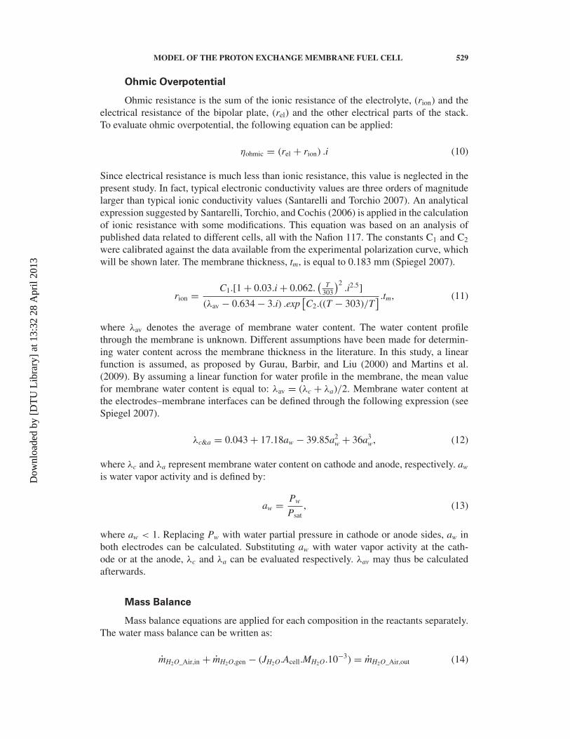
MODEL OF THE PROTON EXCHANGE MEMBRANE FUEL CELL 529

Ohmic Overpotential

Ohmic resistance is the sum of the ionic resistance of the electrolyte, (rion) and theelectrical resistance of the bipolar plate, (rel) and the other electrical parts of the stack.To evaluate ohmic overpotential, the following equation can be applied:

ηohmic = (rel + rion) .i (10)

Since electrical resistance is much less than ionic resistance, this value is neglected in thepresent study. In fact, typical electronic conductivity values are three orders of magnitudelarger than typical ionic conductivity values (Santarelli and Torchio 2007). An analyticalexpression suggested by Santarelli, Torchio, and Cochis (2006) is applied in the calculationof ionic resistance with some modifications. This equation was based on an analysis ofpublished data related to different cells, all with the Nafion 117. The constants C1 and C2

were calibrated against the data available from the experimental polarization curve, whichwill be shown later. The membrane thickness, tm, is equal to 0.183 mm (Spiegel 2007).

rion = C1.[1 + 0.03.i + 0.062.(

T303

)2.i2.5]

(λav − 0.634 − 3.i) .exp[C2.((T − 303)/T

] .tm, (11)

where λav denotes the average of membrane water content. The water content profilethrough the membrane is unknown. Different assumptions have been made for determin-ing water content across the membrane thickness in the literature. In this study, a linearfunction is assumed, as proposed by Gurau, Barbir, and Liu (2000) and Martins et al.(2009). By assuming a linear function for water profile in the membrane, the mean valuefor membrane water content is equal to: λav = (λc + λa)/2. Membrane water content atthe electrodes–membrane interfaces can be defined through the following expression (seeSpiegel 2007).

λc&a = 0.043 + 17.18aw − 39.85a2w + 36a3

w, (12)

where λc and λa represent membrane water content on cathode and anode, respectively. aw

is water vapor activity and is defined by:

aw = Pw

Psat, (13)

where aw < 1. Replacing Pw with water partial pressure in cathode or anode sides, aw inboth electrodes can be calculated. Substituting aw with water vapor activity at the cath-ode or at the anode, λc and λa can be evaluated respectively. λav may thus be calculatedafterwards.

Mass Balance

Mass balance equations are applied for each composition in the reactants separately.The water mass balance can be written as:

mH2O_Air,in + mH2O,gen − (JH2O.Acell.MH2O.10−3) = mH2O_Air,out (14)

Dow

nloa

ded

by [

DT

U L

ibra

ry]

at 1

3:32

28

Apr

il 20

13

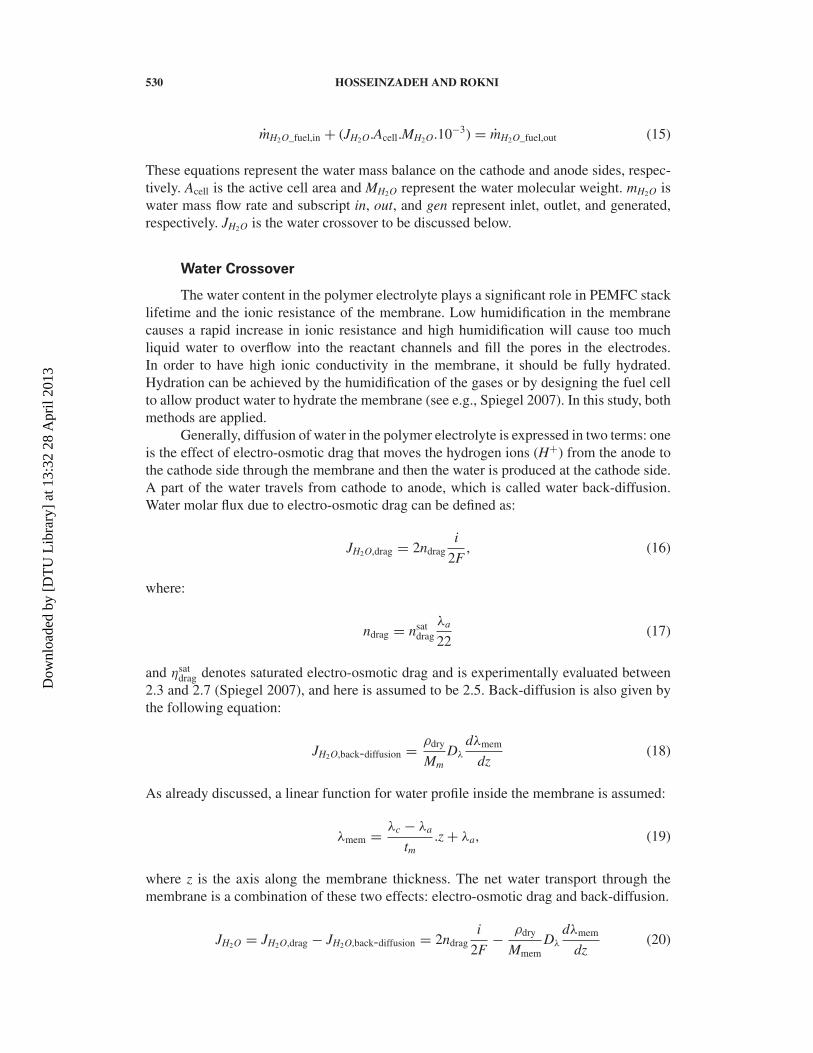
530 HOSSEINZADEH AND ROKNI

mH2O_fuel,in + (JH2O.Acell.MH2O.10−3) = mH2O_fuel,out (15)

These equations represent the water mass balance on the cathode and anode sides, respec-tively. Acell is the active cell area and MH2O represent the water molecular weight. mH2O iswater mass flow rate and subscript in, out, and gen represent inlet, outlet, and generated,respectively. JH2O is the water crossover to be discussed below.

Water Crossover

The water content in the polymer electrolyte plays a significant role in PEMFC stacklifetime and the ionic resistance of the membrane. Low humidification in the membranecauses a rapid increase in ionic resistance and high humidification will cause too muchliquid water to overflow into the reactant channels and fill the pores in the electrodes.In order to have high ionic conductivity in the membrane, it should be fully hydrated.Hydration can be achieved by the humidification of the gases or by designing the fuel cellto allow product water to hydrate the membrane (see e.g., Spiegel 2007). In this study, bothmethods are applied.

Generally, diffusion of water in the polymer electrolyte is expressed in two terms: oneis the effect of electro-osmotic drag that moves the hydrogen ions (H+) from the anode tothe cathode side through the membrane and then the water is produced at the cathode side.A part of the water travels from cathode to anode, which is called water back-diffusion.Water molar flux due to electro-osmotic drag can be defined as:

JH2O,drag = 2ndragi

2F, (16)

where:

ndrag = nsatdrag

λa

22(17)

and ηsatdrag denotes saturated electro-osmotic drag and is experimentally evaluated between

2.3 and 2.7 (Spiegel 2007), and here is assumed to be 2.5. Back-diffusion is also given bythe following equation:

JH2O,back-diffusion = ρdry

MmDλ

dλmem

dz(18)

As already discussed, a linear function for water profile inside the membrane is assumed:

λmem = λc − λa

tm.z + λa, (19)

where z is the axis along the membrane thickness. The net water transport through themembrane is a combination of these two effects: electro-osmotic drag and back-diffusion.

JH2O = JH2O,drag − JH2O,back-diffusion = 2ndragi

2F− ρdry

MmemDλ

dλmem

dz(20)

Dow

nloa

ded

by [

DT

U L

ibra

ry]

at 1

3:32

28

Apr

il 20

13

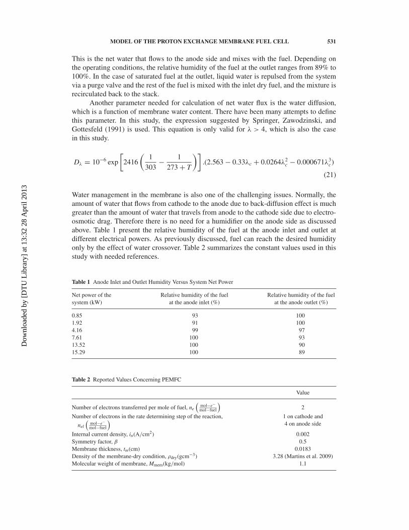
MODEL OF THE PROTON EXCHANGE MEMBRANE FUEL CELL 531

This is the net water that flows to the anode side and mixes with the fuel. Depending onthe operating conditions, the relative humidity of the fuel at the outlet ranges from 89% to100%. In the case of saturated fuel at the outlet, liquid water is repulsed from the systemvia a purge valve and the rest of the fuel is mixed with the inlet dry fuel, and the mixture isrecirculated back to the stack.

Another parameter needed for calculation of net water flux is the water diffusion,which is a function of membrane water content. There have been many attempts to definethis parameter. In this study, the expression suggested by Springer, Zawodzinski, andGottesfeld (1991) is used. This equation is only valid for λ > 4, which is also the casein this study.

Dλ = 10−6 exp

[2416

(1

303− 1

273 + T

)].(2.563 − 0.33λc + 0.0264λ2

c − 0.000671λ3c)

(21)

Water management in the membrane is also one of the challenging issues. Normally, theamount of water that flows from cathode to the anode due to back-diffusion effect is muchgreater than the amount of water that travels from anode to the cathode side due to electro-osmotic drag. Therefore there is no need for a humidifier on the anode side as discussedabove. Table 1 present the relative humidity of the fuel at the anode inlet and outlet atdifferent electrical powers. As previously discussed, fuel can reach the desired humidityonly by the effect of water crossover. Table 2 summarizes the constant values used in thisstudy with needed references.

Table 1 Anode Inlet and Outlet Humidity Versus System Net Power

Net power of thesystem (kW)

Relative humidity of the fuelat the anode inlet (%)

Relative humidity of the fuelat the anode outlet (%)

0.85 93 1001.92 91 1004.16 99 977.61 100 9313.52 100 9015.29 100 89

Table 2 Reported Values Concerning PEMFC

Value

Number of electrons transferred per mole of fuel, ne

(mol−e−mol−fuel

)2

Number of electrons in the rate determining step of the reaction,

nel

(mol−e−mol−fuel

) 1 on cathode and4 on anode side

Internal current density, in(A/cm2) 0.002Symmetry factor, β 0.5Membrane thickness, tm(cm) 0.0183Density of the membrane-dry condition, ρdry(gcm−3) 3.28 (Martins et al. 2009)Molecular weight of membrane, Mmem(kg/mol) 1.1

Dow

nloa

ded

by [

DT

U L

ibra

ry]

at 1

3:32

28

Apr

il 20

13

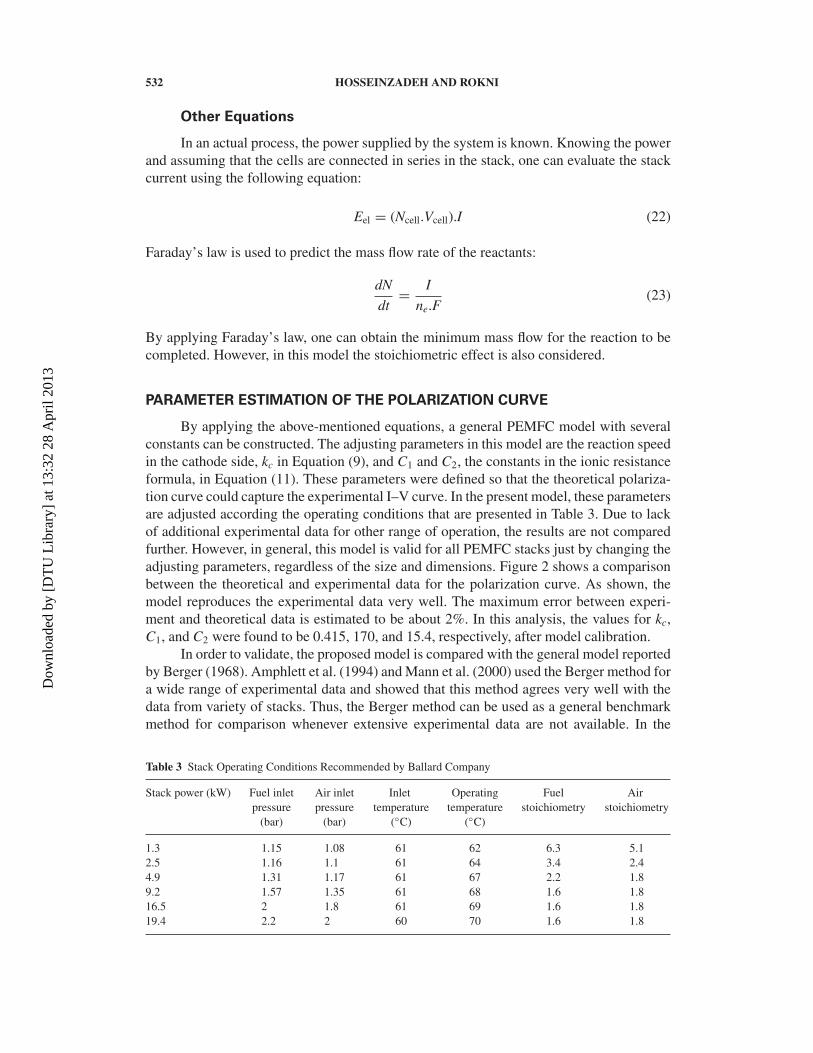
532 HOSSEINZADEH AND ROKNI

Other Equations

In an actual process, the power supplied by the system is known. Knowing the powerand assuming that the cells are connected in series in the stack, one can evaluate the stackcurrent using the following equation:

Eel = (Ncell.Vcell).I (22)

Faraday’s law is used to predict the mass flow rate of the reactants:

dN

dt= I

ne.F(23)

By applying Faraday’s law, one can obtain the minimum mass flow for the reaction to becompleted. However, in this model the stoichiometric effect is also considered.

PARAMETER ESTIMATION OF THE POLARIZATION CURVE

By applying the above-mentioned equations, a general PEMFC model with severalconstants can be constructed. The adjusting parameters in this model are the reaction speedin the cathode side, kc in Equation (9), and C1 and C2, the constants in the ionic resistanceformula, in Equation (11). These parameters were defined so that the theoretical polariza-tion curve could capture the experimental I–V curve. In the present model, these parametersare adjusted according the operating conditions that are presented in Table 3. Due to lackof additional experimental data for other range of operation, the results are not comparedfurther. However, in general, this model is valid for all PEMFC stacks just by changing theadjusting parameters, regardless of the size and dimensions. Figure 2 shows a comparisonbetween the theoretical and experimental data for the polarization curve. As shown, themodel reproduces the experimental data very well. The maximum error between experi-ment and theoretical data is estimated to be about 2%. In this analysis, the values for kc,C1, and C2 were found to be 0.415, 170, and 15.4, respectively, after model calibration.

In order to validate, the proposed model is compared with the general model reportedby Berger (1968). Amphlett et al. (1994) and Mann et al. (2000) used the Berger method fora wide range of experimental data and showed that this method agrees very well with thedata from variety of stacks. Thus, the Berger method can be used as a general benchmarkmethod for comparison whenever extensive experimental data are not available. In the

Table 3 Stack Operating Conditions Recommended by Ballard Company

Stack power (kW) Fuel inletpressure

(bar)

Air inletpressure

(bar)

Inlettemperature

(C)

Operatingtemperature

(C)

Fuelstoichiometry

Airstoichiometry

1.3 1.15 1.08 61 62 6.3 5.12.5 1.16 1.1 61 64 3.4 2.44.9 1.31 1.17 61 67 2.2 1.89.2 1.57 1.35 61 68 1.6 1.816.5 2 1.8 61 69 1.6 1.819.4 2.2 2 60 70 1.6 1.8

Dow

nloa

ded

by [

DT

U L

ibra

ry]

at 1

3:32

28

Apr

il 20

13

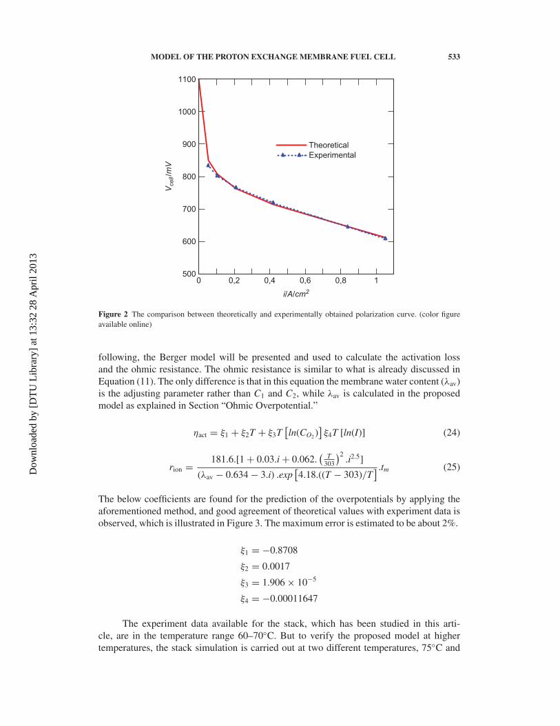
MODEL OF THE PROTON EXCHANGE MEMBRANE FUEL CELL 533

i/A/cm2

Vce

ll/m

V

0 0,2 0,4 0,6 0,8 1500

600

700

800

900

1000

1100

Theoretical

Experimental

Figure 2 The comparison between theoretically and experimentally obtained polarization curve. (color figureavailable online)

following, the Berger model will be presented and used to calculate the activation lossand the ohmic resistance. The ohmic resistance is similar to what is already discussed inEquation (11). The only difference is that in this equation the membrane water content (λav)is the adjusting parameter rather than C1 and C2, while λav is calculated in the proposedmodel as explained in Section “Ohmic Overpotential.”

ηact = ξ1 + ξ2T + ξ3T[ln(CO2 )

]ξ4T [ln(I)] (24)

rion = 181.6.[1 + 0.03.i + 0.062.(

T303

)2.i2.5]

(λav − 0.634 − 3.i) .exp[4.18.((T − 303)/T

] .tm (25)

The below coefficients are found for the prediction of the overpotentials by applying theaforementioned method, and good agreement of theoretical values with experiment data isobserved, which is illustrated in Figure 3. The maximum error is estimated to be about 2%.

ξ1 = −0.8708

ξ2 = 0.0017

ξ3 = 1.906 × 10−5

ξ4 = −0.00011647

The experiment data available for the stack, which has been studied in this arti-cle, are in the temperature range 60–70C. But to verify the proposed model at highertemperatures, the stack simulation is carried out at two different temperatures, 75C and

Dow

nloa

ded

by [

DT

U L

ibra

ry]

at 1

3:32

28

Apr

il 20

13

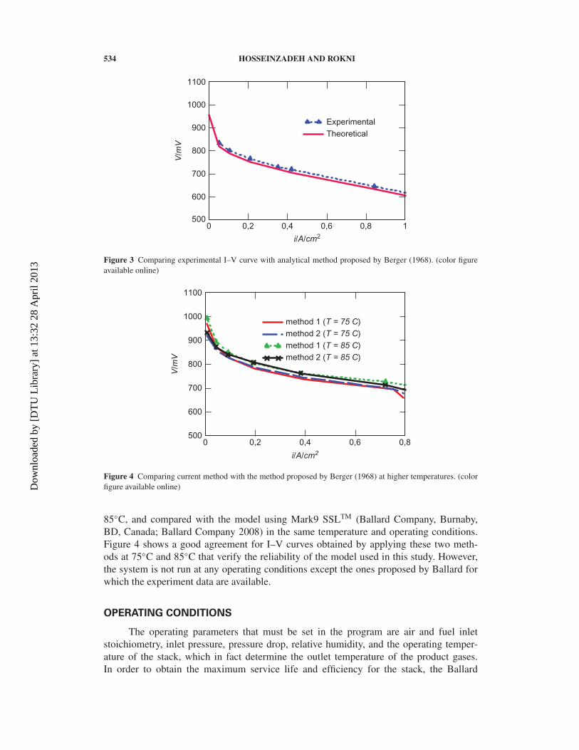
534 HOSSEINZADEH AND ROKNI

i/A/cm2

V/m

V

0 0,2 0,4 0,6 0,8 1500

600

700

800

900

1000

1100

Experimental

Theoretical

Figure 3 Comparing experimental I–V curve with analytical method proposed by Berger (1968). (color figureavailable online)

i/A/cm2

V/m

V

0 0,2 0,4 0,6 0,8500

600

700

800

900

1000

1100

method 1 (T = 75 C)

method 2 (T = 75 C)

method 1 (T = 85 C)

method 2 (T = 85 C)

Figure 4 Comparing current method with the method proposed by Berger (1968) at higher temperatures. (colorfigure available online)

85C, and compared with the model using Mark9 SSLTM (Ballard Company, Burnaby,BD, Canada; Ballard Company 2008) in the same temperature and operating conditions.Figure 4 shows a good agreement for I–V curves obtained by applying these two meth-ods at 75C and 85C that verify the reliability of the model used in this study. However,the system is not run at any operating conditions except the ones proposed by Ballard forwhich the experiment data are available.

OPERATING CONDITIONS

The operating parameters that must be set in the program are air and fuel inletstoichiometry, inlet pressure, pressure drop, relative humidity, and the operating temper-ature of the stack, which in fact determine the outlet temperature of the product gases.In order to obtain the maximum service life and efficiency for the stack, the Ballard

Dow

nloa

ded

by [

DT

U L

ibra

ry]

at 1

3:32

28

Apr

il 20

13

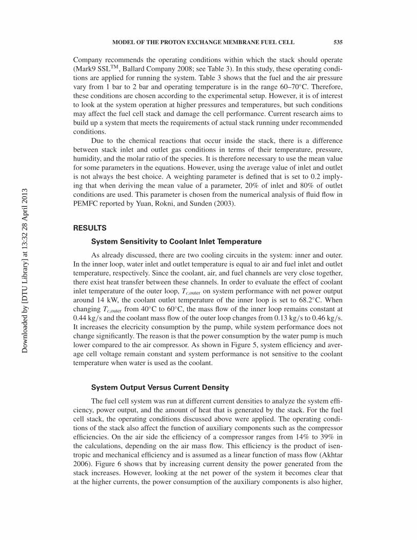
MODEL OF THE PROTON EXCHANGE MEMBRANE FUEL CELL 535

Company recommends the operating conditions within which the stack should operate(Mark9 SSLTM, Ballard Company 2008; see Table 3). In this study, these operating condi-tions are applied for running the system. Table 3 shows that the fuel and the air pressurevary from 1 bar to 2 bar and operating temperature is in the range 60–70C. Therefore,these conditions are chosen according to the experimental setup. However, it is of interestto look at the system operation at higher pressures and temperatures, but such conditionsmay affect the fuel cell stack and damage the cell performance. Current research aims tobuild up a system that meets the requirements of actual stack running under recommendedconditions.

Due to the chemical reactions that occur inside the stack, there is a differencebetween stack inlet and outlet gas conditions in terms of their temperature, pressure,humidity, and the molar ratio of the species. It is therefore necessary to use the mean valuefor some parameters in the equations. However, using the average value of inlet and outletis not always the best choice. A weighting parameter is defined that is set to 0.2 imply-ing that when deriving the mean value of a parameter, 20% of inlet and 80% of outletconditions are used. This parameter is chosen from the numerical analysis of fluid flow inPEMFC reported by Yuan, Rokni, and Sunden (2003).

RESULTS

System Sensitivity to Coolant Inlet Temperature

As already discussed, there are two cooling circuits in the system: inner and outer.In the inner loop, water inlet and outlet temperature is equal to air and fuel inlet and outlettemperature, respectively. Since the coolant, air, and fuel channels are very close together,there exist heat transfer between these channels. In order to evaluate the effect of coolantinlet temperature of the outer loop, Tc,outer on system performance with net power outputaround 14 kW, the coolant outlet temperature of the inner loop is set to 68.2C. Whenchanging Tc,outer from 40C to 60C, the mass flow of the inner loop remains constant at0.44 kg/s and the coolant mass flow of the outer loop changes from 0.13 kg/s to 0.46 kg/s.It increases the elecricity consumption by the pump, while system performance does notchange significantly. The reason is that the power consumption by the water pump is muchlower compared to the air compressor. As shown in Figure 5, system efficiency and aver-age cell voltage remain constant and system performance is not sensitive to the coolanttemperature when water is used as the coolant.

System Output Versus Current Density

The fuel cell system was run at different current densities to analyze the system effi-ciency, power output, and the amount of heat that is generated by the stack. For the fuelcell stack, the operating conditions discussed above were applied. The operating condi-tions of the stack also affect the function of auxiliary components such as the compressorefficiencies. On the air side the efficiency of a compressor ranges from 14% to 39% inthe calculations, depending on the air mass flow. This efficiency is the product of isen-tropic and mechanical efficiency and is assumed as a linear function of mass flow (Akhtar2006). Figure 6 shows that by increasing current density the power generated from thestack increases. However, looking at the net power of the system it becomes clear thatat the higher currents, the power consumption of the auxiliary components is also higher,

Dow

nloa

ded

by [

DT

U L

ibra

ry]

at 1

3:32

28

Apr

il 20

13

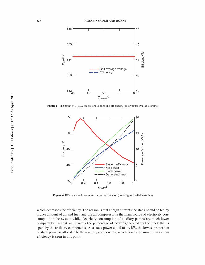
536 HOSSEINZADEH AND ROKNI

Tc,outer/°c

Vce

ll/m

V

Effic

iency/%

40 45 50 55 6042652

43653

44654

45655

46656

Cell average voltageEfficiency

Figure 5 The effect of Tc,outer on system voltage and efficiency. (color figure available online)

i/A/cm2

Effic

iency/%

Pow

er

kw

& E

nerg

y/k

J/s

0 0,2 0,4 0,6 0,8 1035

540

1045

1550

2055

System efficiencyNet powerStack powerGenerated heat

Figure 6 Efficiency and power versus current density. (color figure available online)

which decreases the efficiency. The reason is that at high currents the stack shoud be fed byhigher amount of air and fuel, and the air compressor is the main source of electricity con-sumption in the system while electricity consumption of auxilary pumps are much lowercomparably. Table 4 summarizes the percentage of power generated by the stack that isspent by the axiluary components. At a stack power equal to 4.9 kW, the lowest proportionof stack power is allocated to the auxilary components, which is why the maximum systemefficiency is seen in this point.

Dow

nloa

ded

by [

DT

U L

ibra

ry]

at 1

3:32

28

Apr

il 20

13

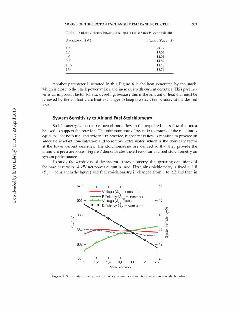
MODEL OF THE PROTON EXCHANGE MEMBRANE FUEL CELL 537

Table 4 Ratio of Axiluary Power Consumption to the Stack Power Production

Stack power (kW) Pauxilary/Pstack (%)

1.3 29.322.5 19.624.9 12.919.2 14.8716.5 18.5819.4 18.78

Another parameter illustrated in this Figure 6 is the heat generated by the stack,which is close to the stack power values and increases with current densities. This parame-ter is an important factor for stack cooling, because this is the amount of heat that must beremoved by the coolant via a heat exchanger to keep the stack temperature at the desiredlevel.

System Sensitivity to Air and Fuel Stoichiometry

Stoichiometry is the ratio of actual mass flow to the requaired mass flow that mustbe used to support the reaction. The minimum mass flow ratio to complete the reaction isequal to 1 for both fuel and oxidant. In practice, higher mass flow is required to provide anadequate reactant concentration and to remove extra water, which is the dominant factorat the lower current densities. The stoichiometries are defined so that they provide theminimum pressure losses. Figure 7 demonstrates the effect of air and fuel stoichiometry onsystem performance.

To study the sensitivity of the system to stoichiometry, the operating conditions ofthe base case with 14 kW net power output is used. First, air stoichiometry is fixed at 1.8(So2 = constant in the figure) and fuel stoichiometry is changed from 1 to 2.2 and then in

Stoichiometry

Vce

ll/m

V

Syste

m e

ffic

iency/%

1 1,2 1,4 1,6 1,8 2 2,240660

42662

44664

46666

48668

50670

Voltage (SO2 = constant)

Efficiency (SO2 = constant)

Voltage (SH2= constant)

Efficiency (SH2 = constant)

Figure 7 Sensitivity of voltage and efficiency versus stoichiometry. (color figure available online)

Dow

nloa

ded

by [

DT

U L

ibra

ry]

at 1

3:32

28

Apr

il 20

13

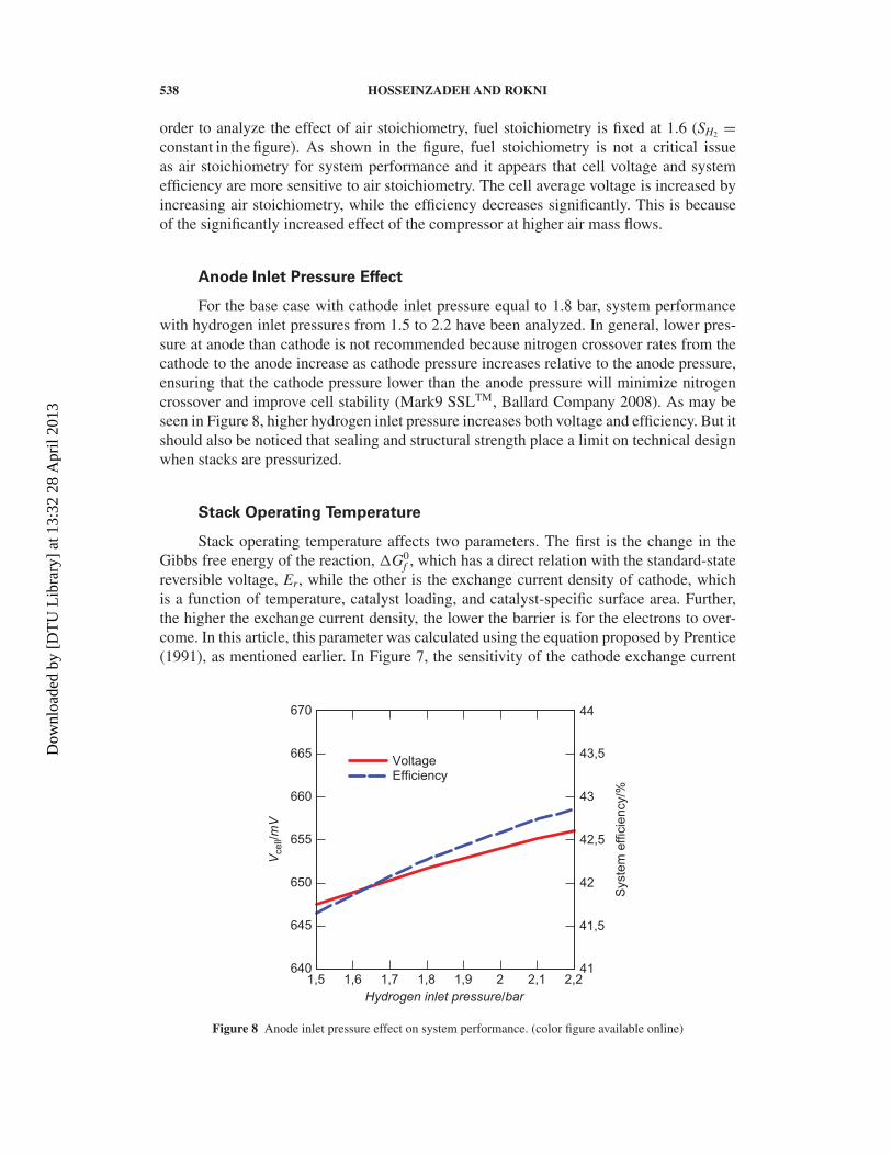
538 HOSSEINZADEH AND ROKNI

order to analyze the effect of air stoichiometry, fuel stoichiometry is fixed at 1.6 (SH2 =constant in the figure). As shown in the figure, fuel stoichiometry is not a critical issueas air stoichiometry for system performance and it appears that cell voltage and systemefficiency are more sensitive to air stoichiometry. The cell average voltage is increased byincreasing air stoichiometry, while the efficiency decreases significantly. This is becauseof the significantly increased effect of the compressor at higher air mass flows.

Anode Inlet Pressure Effect

For the base case with cathode inlet pressure equal to 1.8 bar, system performancewith hydrogen inlet pressures from 1.5 to 2.2 have been analyzed. In general, lower pres-sure at anode than cathode is not recommended because nitrogen crossover rates from thecathode to the anode increase as cathode pressure increases relative to the anode pressure,ensuring that the cathode pressure lower than the anode pressure will minimize nitrogencrossover and improve cell stability (Mark9 SSLTM, Ballard Company 2008). As may beseen in Figure 8, higher hydrogen inlet pressure increases both voltage and efficiency. But itshould also be noticed that sealing and structural strength place a limit on technical designwhen stacks are pressurized.

Stack Operating Temperature

Stack operating temperature affects two parameters. The first is the change in theGibbs free energy of the reaction, G0

f , which has a direct relation with the standard-statereversible voltage, Er, while the other is the exchange current density of cathode, whichis a function of temperature, catalyst loading, and catalyst-specific surface area. Further,the higher the exchange current density, the lower the barrier is for the electrons to over-come. In this article, this parameter was calculated using the equation proposed by Prentice(1991), as mentioned earlier. In Figure 7, the sensitivity of the cathode exchange current

Hydrogen inlet pressure/bar

Vce

ll/m

V

Syste

m e

ffic

ien

cy/%

1,5 1,6 1,7 1,8 1,9 2 2,1 2,241640

41,5645

42650

42,5655

43660

43,5665

44670

VoltageEfficiency

Figure 8 Anode inlet pressure effect on system performance. (color figure available online)

Dow

nloa

ded

by [

DT

U L

ibra

ry]

at 1

3:32

28

Apr

il 20

13

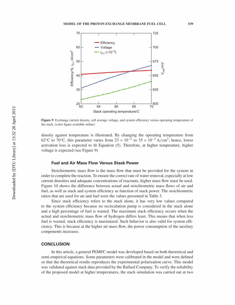
MODEL OF THE PROTON EXCHANGE MEMBRANE FUEL CELL 539

Stack operating temperature/C

Effic

iency/%

, i 0

,c /A

/cm

2

Vce

ll/m

V

62 64 66 68 7060020

62530

65040

67550

70060

72570

Efficiency

Voltage

i0,c (×10–5)

Figure 9 Exchange current density, cell average voltage, and system efficiency versus operating temperature ofthe stack. (color figure available online)

density against temperature is illustrated. By changing the operating temperature from62C to 70C, this parameter varies from 23 × 10−5 to 35 × 10−5 A/cm2; hence, loweractivation loss is expected to fit Equation (5). Therefore, at higher temperature, highervoltage is expected (see Figure 9)

Fuel and Air Mass Flow Versus Stack Power

Stoichiometric mass flow is the mass flow that must be provided for the system inorder to complete the reaction. To ensure the correct rate of water removal, especially at lowcurrent densities and adequate concentrations of reactants, higher mass flow must be used.Figure 10 shows the difference between actual and stoichiometric mass flows of air andfuel, as well as stack and system efficiency as function of stack power. The stoichiometricratios that are used for air and fuel were the values presented in Table 3.

Since stack efficiency refers to the stack alone, it has very low values comparedto the system efficiency because no recirculation pump is considered in the stack aloneand a high percentage of fuel is wasted. The maximum stack efficiency occurs when theactual and stoichiometric mass flow of hydrogen differs least. This means that when lessfuel is wasted, stack efficiency is maximized. Such behavior is also valid for system effi-ciency. This is because at the higher air mass flow, the power consumption of the auxilarycomponents increases.

CONCLUSION

In this article, a general PEMFC model was developed based on both theoretical andsemi-empirical equations. Some parameters were calibrated in the model and were definedso that the theoretical results reproduces the experimental polarization curve. This modelwas validated against stack data provided by the Ballard Company. To verify the reliabilityof the proposed model at higher temperatures, the stack simulation was carried out at two

Dow

nloa

ded

by [

DT

U L

ibra

ry]

at 1

3:32

28

Apr

il 20

13

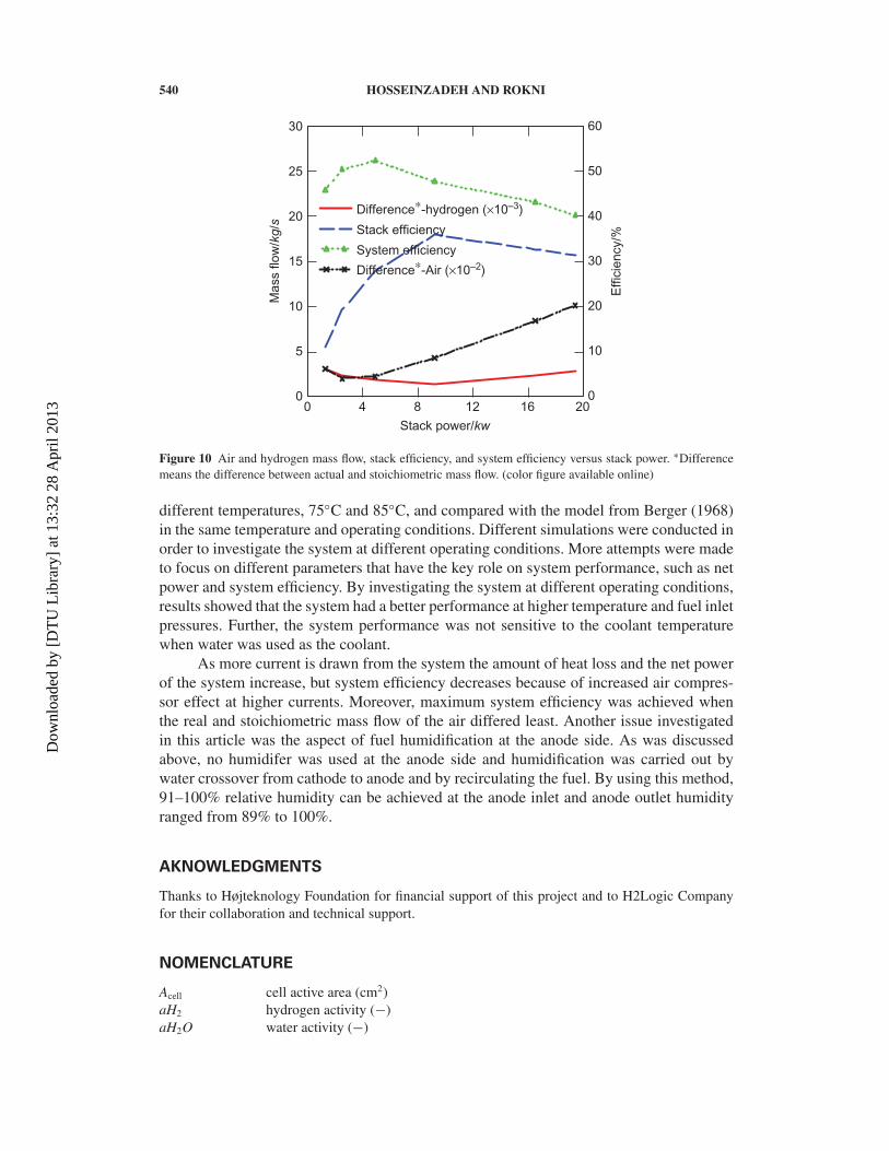
540 HOSSEINZADEH AND ROKNI

Stack power/kw

Mass flo

w/k

g/s

Effic

iency/%

0 4 8 12 16 2000

105

2010

3015

4020

5025

6030

Difference∗-hydrogen (×10–3)

Stack efficiency

System efficiency

Difference∗-Air (×10–2)

Figure 10 Air and hydrogen mass flow, stack efficiency, and system efficiency versus stack power. ∗Differencemeans the difference between actual and stoichiometric mass flow. (color figure available online)

different temperatures, 75C and 85C, and compared with the model from Berger (1968)in the same temperature and operating conditions. Different simulations were conducted inorder to investigate the system at different operating conditions. More attempts were madeto focus on different parameters that have the key role on system performance, such as netpower and system efficiency. By investigating the system at different operating conditions,results showed that the system had a better performance at higher temperature and fuel inletpressures. Further, the system performance was not sensitive to the coolant temperaturewhen water was used as the coolant.

As more current is drawn from the system the amount of heat loss and the net powerof the system increase, but system efficiency decreases because of increased air compres-sor effect at higher currents. Moreover, maximum system efficiency was achieved whenthe real and stoichiometric mass flow of the air differed least. Another issue investigatedin this article was the aspect of fuel humidification at the anode side. As was discussedabove, no humidifer was used at the anode side and humidification was carried out bywater crossover from cathode to anode and by recirculating the fuel. By using this method,91–100% relative humidity can be achieved at the anode inlet and anode outlet humidityranged from 89% to 100%.

AKNOWLEDGMENTS

Thanks to Højteknology Foundation for financial support of this project and to H2Logic Companyfor their collaboration and technical support.

NOMENCLATURE

Acell cell active area (cm2)aH2 hydrogen activity (−)aH2O water activity (−)

Dow

nloa

ded

by [

DT

U L

ibra

ry]

at 1

3:32

28

Apr

il 20

13

MODEL OF THE PROTON EXCHANGE MEMBRANE FUEL CELL 541

aO2 oxygen activity (−)aw water vapour activity (−)CO2 oxygen concentration at the cathode (mol/cm3)C1 Constant (−)C2 Constant (−)Dλ water diffusion coefficient (cm2/s)E theoretical voltage (V)Eel stack power (W)E0 open circuit voltage (V)F Faraday’s constant ( C

mol )I current (A)i current density (A/cm2)in internal current density (A/cm2)i0 exchange current density (A/cm2)i0,a anode exchange current density (A/cm2)i0,c cathode exchange current density (A/cm2)JH2O,back-diffusion back-diffusion water flux, mol/(scm2)JH2O,drag electro-osmotic drag water flux, mol/(scm2)ka anode reaction rate, mol/(scm2)kc cathode reaction rate, mol/(scm2)mH2O Water mass flow rate (kg/s)MH2O molecular weight of water (kg/mol)Mmem molecular weight of membrane (kg/mol)N hydrogen molar flow (mol/s)Ncell number of cells (−)ndrag electro-osmotic drag (−)nsat

drag saturated electro-osmotic drag (−)

ne number of electrons transferred per mole of fuel ( mol−e−mol−fuel )

nel Number of electrons in the rate determining step of the reaction (−)Psat saturated pressure of water (bar)Pw water vapor pressure (bar)R Estefan-Boltzmann constant (J/molK)rel electrical resistance (cm2)rion ionic resistance (cm)rohmic ohmic resistance (cm2)T Temperature (K)Tc,outer coolant inlet temperature of the outer loop (C)tm membrane thickness (cm)Vcell cell average voltage (V)

Greek letters∝a anode transfer coefficienct, (−)αc cathode transfer coefficienct, (−)β symmetry factor (−)λmem membrane water content (−)λa anode water content (−)λav membrane average water content (−)λc cathode water content (−)λc&a electrode/membrane water content (−)ρdry membrane density (g/cm3)ηact activation overpotential (V)

Dow

nloa

ded

by [

DT

U L

ibra

ry]

at 1

3:32

28

Apr

il 20

13

542 HOSSEINZADEH AND ROKNI

ηact,a anode activation overpotential (V)ηact,c cathode activation overpotential (V)ηconc concentration overpotential (V)ηohm ohmic overpotential (V)ξ empirical coefficient for calculation of activation overvoltageG0

f change in Gibbs free energy (J/molK)

REFERENCES

Ahluwalia, R.K., and X. Wang. 2005. Direct hydrogen fuel cell systems for hybrid vehicles. Journalof Power Sources 139: 152–64.

Akhtar, M.S. 2006. Determining the real performance of centrifugal compressors operating in oil &gas production facilities. Paper presented at the 9th European Fluid Machinary Congress on“Applying the Latest Technology to New and Existing Process Equipment,” April 23–26 , inThe Hague, The Netherlands, pp. 127–44.

Amphlett, J.C., R.M. Baumert, R.F. Mann, B.A. Peppley, P.R. Roberge, and A. Rodrigues. 1994.Parametric modelling of the performance of a 5kW proton-exchange membrane fuel cell stack.Journal of Power Sources 49:349–56.

Ballard Company. (2008). Mark9 SSLTM: Product manual and integration guide. Burnaby, Canada:Ballard Company.

Berger, C. 1968. Handbook of fuel cell technology. Engelwood, NJ: Prentice Hall.Corbo, P., F. Migliardini, and O. Veneri. 2007. Experimental analysis and management issues of

a hydrogen fuel cell system for stationary and mobile application. Energy Conversion andManagement 48:2365–74.

Cordner, M., M. Matian, G.J. Offer, T. Hanten, E. Spofforth-Jones, S. Tippetts, A. Agrawal, L.Bannar-Martin, L. Harito, A. Johnson, R. Clague, F. Marquis, A. Heyes, Y. Hardalupas, andN.P. Brandon. 2010. Designing, building, testing and racing a low-cost fuel cell range extenderfor a motorsport application. Journal of Power Sources 195:7838–48.

Danilov, V.A., and M.O. Tade. 2010. An alternative way of estimating anodic and cathodic transfercoefficients from PEMFC polarization curves. Chemical Engineering Journal 156:496–9.

Gurau, V., F. Barbir, and H. Liu. 2000. An analytical solution of a half-cell model for PEM fuel cells.Journal of the Electrochemical Society 147:2468–77.

Haji, S. 2011. Analytical modeling of PEM fuel cell I–V curve. Renewable Energy 36:451–8.Larminie, A.D. 2000. Fuel cell systems explained. Chichester: John Wiley.Liu, F., G. Lu, and C.Y. Wang. 2006. Water transport coefficient distribution through the membrane

in a polymer electrolyte fuel cell. Journal of Membrane Science 287:126–31.Mann, R.F., J.C. Amphlett, M.A.I. Hooper, H.M. Jensen, B.A. Peppley, and P.R. Roberge. 2000.

Development and application of a generalised steady-state electrochemical model for a PEMfuel cell. Journal of Power Sources 86:173–80.

Martins, L.S., J.E.F.C. Gardolinski, J.V.C. Vargas, J.C. Ordonez, S.C. Amico, and M.M.C. Forte.2009. The experimental validation of a simplified PEMFC simulation model for design andoptimization purposes. Applied Thermal Engineering 29: 3036–48.

Matamoros, L., and D. Bruggemann. 2007. Concentration and ohmic losses in free-breathingPEMFC. Journal of Power Sources 173: 367–74.

Patel, S., A.S. Bansode, T. Sundararajan, and S.K. Das. 2008. The performance analysis of a multi-duct proton exchange membrane fuel cell cathode. International Journal of Green Energy 5:35–54.

Prentice, G. 1991. Electrochemical engineering principles. Houston, TX: Prentice Hall International.Santarelli, M.G., and M.F. Torchio. 2007. Experimental analysis of the effects of the operating

variables on the performance of a single PEMFC. Energy Conversion and Management 48:40–51.

Dow

nloa

ded

by [

DT

U L

ibra

ry]

at 1

3:32

28

Apr

il 20

13

MODEL OF THE PROTON EXCHANGE MEMBRANE FUEL CELL 543

Santarelli, M.G., M.F. Torchio, and P. Cochis. 2006. Parameters estimation of a PEM fuel cell polar-ization curve and analysis of their behavior with temperature. Journal of Power Sources 159:824–35.

Spiegel, C. 2007. Designing and building fuel cells. New York: McGraw-Hill.Spinelli, P., C. Francia, E.P. Ambrosio, and M. Lucariello. 2008. Semi-empirical evaluation of

PEMFC electro-catalytic activity. Journal of Power Sources 178: 517–24.Springer, T.E., T.A. Zawodzinski, and S. Gottesfeld. 1991. Polymer electrolyte fuel cell model.

Electrochemical Society 138: 2334–42.Wang, J., J. Yan, J. Yuan, and B. Sundén. 2011. On flow maldistribution in PEMFC stacks.

International Journal of Green Energy 8: 585–606.Yan, W.M., H.S. Chu, J.Y. Chen, C.Y. Soong, and F. Chen. 2006. Transient analysis of water transport

in PEM fuel cells. Journal of Power Sources 162: 1147–56.Yu, X., B. Zhou, and A. Sobiesiak. 2005. Water and thermal management for Ballard PEM fuel cell

stack. Journal of Power Sources 147: 184–95.Yuan, J., M. Rokni, and B. Sunden. 2003. A numerical investigation of gas flow and heat transfer in

proton exchange membrane fuel cells. Numerical Heat Transfer 44: 255–80.Yuan, J., and B. Sundén. 2004. Numerical analysis of heat transfer and gas flow in PEM fuel cell ducts

by a generalized extended Darcy model. International Journal of Green Energy 1: 47–63.

Dow

nloa

ded

by [

DT

U L

ibra

ry]

at 1

3:32

28

Apr

il 20

13

Appendix C

Paper II

Thermal and water management of Low Temperature Proton Exchange Membrane FuelCell in fork-lift truck power system

174

Thermal and water management of low temperature Proton ExchangeMembrane Fuel Cell in fork-lift truck power system

Elham Hosseinzadeh a, Masoud Rokni a,⇑, Abid Rabbani a, Henrik Hilleke Mortensen b

a Technical University of Denmark, Dept. of Mechanical Engineering, Thermal Energy Section, 2800 Kgs, Lyngby, Denmarkb H2Logic A/S, Industriparken 34 B, 7400 Herning, Denmark

h i g h l i g h t s

" Developing a general zero dimensional Proton Exchange Membrane Fuel Cell (PEMFC) model for a forklift." System performance with different cooling fluids." Water and thermal management of fuel cell system." Effect of inlet temperature, outlet temperature and temperature gradient on system performance.

a r t i c l e i n f o

Article history:Received 22 August 2012Received in revised form 14 November 2012Accepted 20 November 2012Available online 20 December 2012

Keywords:PEMFuel cellThermal managementWater managementForkliftPower system

a b s t r a c t

A general zero-dimensional Proton Exchange Membrane Fuel Cell (PEMFC) model has been developed forforklift truck application. The balance of plant (BOP) comprises of a compressor, an air humidifier, a set ofheat exchangers and a recirculation pump. Water and thermal management of the fuel cell stack and BOPhas been investigated in this study. The results show that humidification of the inlet air is of great impor-tance. By decreasing the relative humidity of inlet air from 95% to 25%, the voltage can drop by 29%. Inaddition, elevated stack temperature can lead to a higher average cell voltage when membrane is fullyhydrated otherwise it causes a drastic voltage drop in the stack. Furthermore, by substituting liquid waterwith water–ethylene glycol mixture of 50%, the mass flow of coolant increases by about 32–33% in theinner loop and 60–65% in the outer loop for all ranges of current. The system can then be started up atabout 25 C with negligible change in the efficiency.

2012 Elsevier Ltd. All rights reserved.

1. Introduction

Proton Exchange Membrane Fuel Cells (PEMFCs) are consideredas one of the most promising candidates in automotive industrydue to their low operating conditions, high power density andrapid start-up [1–4], but still there are some barriers for commer-cialization of PEM fuel cells such as cost and lifetime [5,6]. The per-formance of PEM fuel cells has been studied from differentperspectives. There are detailed studies on a single cell in the areaof catalysts improvement [7,8], lifetime and degradation [9], mem-brane technology [10], flow channels [11,12], and stack modelingto analyze parametric study of the stack only [13,14]. Otherresearchers investigated performance of a fuel cell integrated withbalance of plant (BOP) [15–17] without studying different types ofcoolant media. The operating temperature of the fuel cell is usuallyin the range of 60–80 C. High temperature in the stack can cause

degradation in the membrane or catalyst while a lower tempera-ture of the stack is not favorable from kinetics point of view, itmight also cause flooding due to lower water saturation pressureat lower temperature which is a major concern for stack watermanagement [18–20]. The important parameters which affect thewater management in the stack consist of: gas flow rates, pressureof the gases, operating temperature of the stack, relative humidityof the gases, gas flow channels as well as gas diffusion layer (GDL)[21]. Many efforts have been exercised with the aim of understand-ing water transport in the PEM fuel cell [22–27], though a few ofthe studies have considered the water transport effect in a realsystem, including PEMFC and BOP.

The main purpose of thermal management is keeping the stackoperating temperature within the desired range [20]. Two factorsare critical in designing a cooling system for PEM fuel cells: firstlythe operating temperature of the stack is limited to 80 C whichmeans that the temperature difference between the ambient airand exhaust gases is too low when comparing to the cooling sys-tem of the conventional internal combustion engine. Secondly,

0306-2619/$ - see front matter 2012 Elsevier Ltd. All rights reserved.http://dx.doi.org/10.1016/j.apenergy.2012.11.048

⇑ Corresponding author.E-mail address: mr@mek.dtu.dk (M. Rokni).

Applied Energy 104 (2013) 434–444

Contents lists available at SciVerse ScienceDirect

Applied Energy

journal homepage: www.elsevier .com/ locate/apenergy

the heat removal by the reactants and products is almost negligibleand the entire waste heat must be removed by a cooling system.These two factors cause a need for a relatively large radiator inautomotive PEMFC systems which is very challenging issue withthe current technology. Raising the operating temperature of thefuel cell could be one way to improve the effectiveness of the cur-rent cooling technologies. Besides, the high temperature fuel cell ismore tolerant against CO contaminations [19,28,29] and it givesthe possibility of using other fuels besides pure hydrogen, thoughdiscussion on high temperature PEMFC is out of scope of this pa-per. Heat generated in the stack may be dissipated by conduction,convection, radiation or phase change [18,30,31]. If the heat is notproperly dissipated by the cooling system, the stack temperatureeventually increases and this will lead to a low relative humidityof the membrane, which decrease the ionic conductivity of themembrane. Therefore water management should also be consid-ered beside the thermal management of the stack. Cooling meth-ods are determined greatly by the size of the fuel cell [30]. Thetypical methods for heat management of the stack are listed as be-low [18,30].

1. Cooling with heat spreaders.2. Cooling with cathode air flow.3. Cooling with separate air flow.4. Liquid cooling.5. Phase change cooling.

Liquid coolants have much higher heat capacity than gas cool-ants, which makes them more efficient for cooling applicationsespecially in PEMFC larger than 5 kW. The most typical liquid cool-ants are deionized water and water–ethylene-glycol mixture.However water–ammonia mixture seems to be an interestingchoice of coolant due to its high heat capacity, but it is saturatedin the present operating conditions (i.e. Tcell 6 80 C andP 6 2.2 bar). Due to wide application of liquid coolants in automo-tive industry, numerous efforts have been made for optimization ofthe cooling system either by finding alternative coolants or opti-mizing cooling channels design and geometry.

In this paper, first a general zero-dimensional PEMFC model forapplication in a 10 kW fork lift truck is presented and validatedagainst available stack data. Then the stack model is applied in acomplete forklift system accompanied with all necessary auxiliary

components. Water and thermal management of the system areinvestigated and discussed in this study in order to better under-stand the system performance and applicability in cold climate con-ditions. Different cooling mediums such as water, water–ethyleneglycol mixture and R134A with two temperature level, 30 and45 C were used and their effect on system performance have beeninvestigated which has not been reported in the literature.

2. Overall system design

Fig. 1 shows a schematic diagram of the PEMFC system ana-lyzed in this study. The system comprises of a PEM stack as theonly source of electric power accompanied by all necessary auxil-iary components which support the fuel cell to operate. These aux-iliary components are known as balance of plants (BOPs) andinclude compressor, pump, an air humidifier and a set of heatexchangers. Fuel cell stack with 20.4 kW nominal power contains110 cells with the cell area equal of 285.88 cm2. Operating temper-ature of the stack is 60–70 C while the pressure range is 1.2–2.2 bar. On the cathode side, air is compressed, pre-cooled andhumidified before entering the cathode side of the stack at a pres-sure less than 2 bar and temperature around 60 C. Fuel used in theanode side is pure hydrogen which is assumed to be pressurizedand stored in a vessel. The amount of hydrogen will be regulatedby using a valve just after the vessel. Hydrogen with a pressure lessthan 2.2 bar and temperature around 48 C enters the anode side ofthe stack. Since all the fuel cannot be reacted inside the stack thenthe rest will be collected and sent back to the anode stream via arecirculation pump.

To prevent dehydration in the membrane, air and fuel must behumidified. In the air side, there is a humidifier which uses some ofthe water vapor from cathode outlet to humidify the inlet air. Therelative humidity of the air prior to stack is set to 95% in the calcu-lations; although other values can be chosen. On the fuel side thereis no humidifier and the fuel can reach the desired humidity bymeans of the water cross-over effect through the membrane fromcathode to anode. Depending on stack power output, anode inlethumidity is between 78% and 100%. This aspect is revisited laterin the paper.

For thermal management, two separate cooling circuits are usedand denoted as inner and outer loops. The inner loop is used for

Nomenclature

Acell cell active area (cm2)aw water vapor activity (–)C1,2 constantCO2 oxygen concentration at the cathode (mol/cm3)Dw water diffusion coefficient (cm2/s)Dk constantE theoretical voltage (V)F Faraday’s constant (C/mol)I current (A)i current density (A/cm2)JH2O;backdiffusion back diffusion water flux (mol/scm2)JH2O;drag electro osmotic drag water flux (mol/scm2)Mmem molecular weight of membrane (kg/mol)_m mass flow rate (kg/s)

n number of electronsndrag electro osmotic drag (–)nsat

drag saturated electro osmotic drag (–)Psat saturated pressure of water (bar)Pw water vapor pressure (bar)

PO2partial pressure of the oxygen

R gas constant (J/mol K)r ohmic resistance (X cm2)rel electrical resistance (X cm2)rion ionic resistance (X cm2)Tcell temperature (K)tm membrane thickness (cm)Vcell cell average voltage (V)

Greek lettersc constantgohmict ohmic overpotential (V)gconc concentration overpotential (V)ka anode water content (–)kc cathode water content (–)kmem membrane water content (–)qdry membrane density (g/cm3)rm membrane conductivity (S/cm)

E. Hosseinzadeh et al. / Applied Energy 104 (2013) 434–444 435

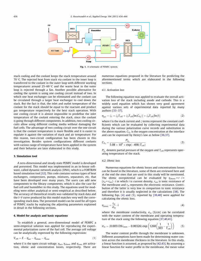
stack cooling and the coolant keeps the stack temperature around70 C. The rejected heat from stack via coolant in the inner loop istransferred to the coolant in the outer loop with different workingtemperatures around 25–60 C and the waste heat in the outerloop is rejected through a fan. Another possible alternative forcooling the system is using one cooling circuit instead of two. Inwhich one heat exchanger can be eliminated and the coolant canbe circulated through a larger heat exchanger to cool down thestack. But the fact is that, the inlet and outlet temperature of thecoolant for the stack should be equal to the reactant and productgas temperature respectively for the best stack operation. Withone cooling circuit it is almost impossible to predefine the inlettemperature of the coolant entering the stack, since the coolantis going through different components. In addition, two cooling cir-cuits allow using different cooling media without damaging thefuel cells. The advantage of two cooling circuit over the one circuitis that the coolant temperature is more flexible and it is easier toregulate it against the variation of stack and air temperature. Forthis reason, two-circuit configuration has been chosen in thisinvestigation. Besides system configurations different coolantswith various range of temperature have been applied in the systemand their behavior are later elaborated in this study.

3. Simulation tool

A zero-dimensional and steady state PEMFC model is developedand presented. This model was implemented in an in-house soft-ware, called dynamic network analysis (DNA), which is a FORTRANbased simulation tool [32]. This code contains various types of heatexchangers, compressors, pumps, mixtures, separators, etc. thathave been developed over many years. The users can add newcomponents to the library components, which is also the case forfuel cell and humidifier in this study. The equations used for mod-eling were either analytical or semi-empirical as described below.The accuracy of theoretical results was validated by stack data andthe I–V curve produced by this model matches very well the corre-sponding stack data. The presented model can be used for all typesof PEMFC stacks by replacing the adjusting parameters explainedin detail in the following sections.

4. Model for analysis and basic equations

To establish a general, zero-dimensional model of PEMFC asemi-empirical solution was applied for reproducing the experi-mental polarization curve of the fuel cell. The average cell voltagecan be analytically expressed by the following expression:

Vcell ¼ E gact gohmic gconc ð1Þ

where E is the open circuit voltage. gact, gohmic and gconc are activa-tion, ohmic and concentration losses, respectively. There are

numerous equations proposed in the literature for predicting theaforementioned terms which are elaborated in the followingsections.

4.1. Activation loss

The following equation was applied to evaluate the overall acti-vation loss of the stack including anode and cathode. This is awidely used equation which has shown very good agreementagainst various sets of experimental data reported by manyauthors [33–37].

gact ¼ n1 þ n2Tcell þ n3Tcell½lnðCO2 Þ þ n4Tcell½lnðIÞ ð2Þ

where I is the stack current and n terms represent the constant coef-ficients which can be evaluated by collecting experimental dataduring the various polarization curve records and substitution inthe above equation. CO2 is the oxygen concentration at the interfaceand can be expressed by Henry’s law as below [36,37].

CO2 ¼PO2

5:08 106 expð498=TcellÞð3Þ

PO2denotes partial pressure of the oxygen and Tcell represents oper-

ating temperature of the stack.

4.2. Ohmic loss

Numerous equations for ohmic losses and concentrations lossescan be found in the literature, some of them are reviewed here andat the end the ones that are used in this study will be mentioned.The ohmic overpotential can be evaluated by gohmic = r i =(rel + rion) i in which i is current density, rion is ionic resistance ofthe membrane and rel represents the electronic resistance. Contri-bution of the latter is very low in comparison to ionic resistanceand therefore it is usually neglected in the calculations [38]. Thefollowing Eqs. (4) and (5), reported by [39,40] were applied forcalculating the ohmic loss.

gohmic ¼tm

rm i ð4Þ

where the membrane conductivity, rm (S/cm) can be correlatedwith the water content of the membrane and operating tempera-ture of the stack using the following equation [37,40,41].

rm ¼ ð0:005139kmem 0:00326Þ exp 12681

303 1

Tcell

ð5Þ

The water content profile through the membrane is unknown.Different assumptions have been made for determining water con-tent across the membrane thickness in the literature. In this study,a linear function is assumed, as proposed by [42,43]. By assuming alinear function for water profile in the membrane, the mean value

Fig. 1. A schematic of PEMFC system.

436 E. Hosseinzadeh et al. / Applied Energy 104 (2013) 434–444

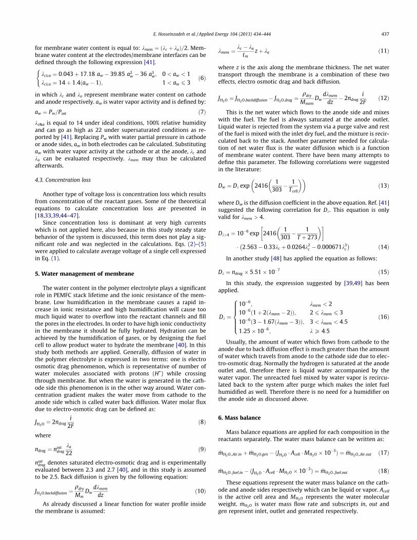
for membrane water content is equal to: kmem ¼ ðkc þ kaÞ=2. Mem-brane water content at the electrodes/membrane interfaces can bedefined through the following expression [41].

kc&a ¼ 0:043þ 17:18 aw 39:85 a2w 36 a3

w; 0 < aw < 1kc&a ¼ 14þ 1:4ðaw 1Þ; 1 < aw 6 3

(ð6Þ

in which kc and ka represent membrane water content on cathodeand anode respectively. aw is water vapor activity and is defined by:

aw ¼ Pw=Psat ð7Þ

kc&a is equal to 14 under ideal conditions, 100% relative humidityand can go as high as 22 under supersaturated conditions as re-ported by [41]. Replacing Pw with water partial pressure in cathodeor anode sides, aw in both electrodes can be calculated. Substitutingaw with water vapor activity at the cathode or at the anode, kc andka can be evaluated respectively. kmem may thus be calculatedafterwards.

4.3. Concentration loss

Another type of voltage loss is concentration loss which resultsfrom concentration of the reactant gases. Some of the theoreticalequations to calculate concentration loss are presented in[18,33,39,44–47].

Since concentration loss is dominant at very high currentswhich is not applied here, also because in this study steady statebehavior of the system is discussed, this term does not play a sig-nificant role and was neglected in the calculations. Eqs. (2)–(5)were applied to calculate average voltage of a single cell expressedin Eq. (1).

5. Water management of membrane

The water content in the polymer electrolyte plays a significantrole in PEMFC stack lifetime and the ionic resistance of the mem-brane. Low humidification in the membrane causes a rapid in-crease in ionic resistance and high humidification will cause toomuch liquid water to overflow into the reactant channels and fillthe pores in the electrodes. In order to have high ionic conductivityin the membrane it should be fully hydrated. Hydration can beachieved by the humidification of gases, or by designing the fuelcell to allow product water to hydrate the membrane [40]. In thisstudy both methods are applied. Generally, diffusion of water inthe polymer electrolyte is expressed in two terms: one is electroosmotic drag phenomenon, which is representative of number ofwater molecules associated with protons (H+) while crossingthrough membrane. But when the water is generated in the cath-ode side this phenomenon is in the other way around. Water con-centration gradient makes the water move from cathode to theanode side which is called water back diffusion. Water molar fluxdue to electro-osmotic drag can be defined as:

JH2O ¼ 2ndragi

2Fð8Þ

where

ndrag ¼ nsatdrag

ka

22ð9Þ

nsatdrag denotes saturated electro-osmotic drag and is experimentally

evaluated between 2.3 and 2.7 [40], and in this study is assumedto be 2.5. Back diffusion is given by the following equation:

JH2O;backdiffusion ¼qdry

MmDw

dkmem

dzð10Þ

As already discussed a linear function for water profile insidethe membrane is assumed:

kmem ¼kc ka

tmzþ ka ð11Þ

where z is the axis along the membrane thickness. The net watertransport through the membrane is a combination of these twoeffects, electro osmotic drag and back diffusion.

JH2O ¼ JH2O;backdiffusion JH2O;drag ¼qdry

MmemDw

dkmem

dz 2ndrag

i2F

ð12Þ

This is the net water which flows to the anode side and mixeswith the fuel. The fuel is always saturated at the anode outlet.Liquid water is rejected from the system via a purge valve and restof the fuel is mixed with the inlet dry fuel, and the mixture is recir-culated back to the stack. Another parameter needed for calcula-tion of net water flux is the water diffusion which is a functionof membrane water content. There have been many attempts todefine this parameter. The following correlations were suggestedin the literature:

Dw ¼ Dk exp 24161

303 1

Tcell

ð13Þ

where Dw is the diffusion coefficient in the above equation. Ref. [41]suggested the following correlation for Dk. This equation is onlyvalid for kmem > 4.

Dk>4 ¼ 106 exp 24161

303 1

T þ 273

2:563 0:33kc þ 0:0264k2c 0:000671k3

c

ð14Þ

In another study [48] has applied the equation as follows:

Dk ¼ ndrag 5:51 107 ð15Þ

In this study, the expression suggested by [39,49] has beenapplied.

Dk ¼

106; kmem < 2106ð1þ 2ðkmem 2ÞÞ; 2 6 kmem 6 3

106ð3 1:67ðkmem 3ÞÞ; 3 < kmem < 4:5

1:25 106; k P 4:5

8>>>><>>>>:

ð16Þ

Usually, the amount of water which flows from cathode to theanode due to back diffusion effect is much greater than the amountof water which travels from anode to the cathode side due to elec-tro-osmotic drag. Normally the hydrogen is saturated at the anodeoutlet and, therefore there is liquid water accompanied by thewater vapor. The unreacted fuel mixed by water vapor is recircu-lated back to the system after purge which makes the inlet fuelhumidified as well. Therefore there is no need for a humidifier onthe anode side as discussed above.

6. Mass balance

Mass balance equations are applied for each composition in thereactants separately. The water mass balance can be written as:

_mH2O Air;in þ _mH2O;gen ðJH2O Acell MH2O 103Þ ¼ _mH2O Air;out ð17Þ

_mH2O fuel;in ðJH2O Acell MH2O 103Þ ¼ _mH2O fuel;out ð18Þ

These equations represent the water mass balance on the cath-ode and anode sides respectively which can be liquid or vapor. Acell

is the active cell area and MH2O represents the water molecularweight. _mH2O is water mass flow rate and subscripts in, out andgen represent inlet, outlet and generated respectively.

E. Hosseinzadeh et al. / Applied Energy 104 (2013) 434–444 437

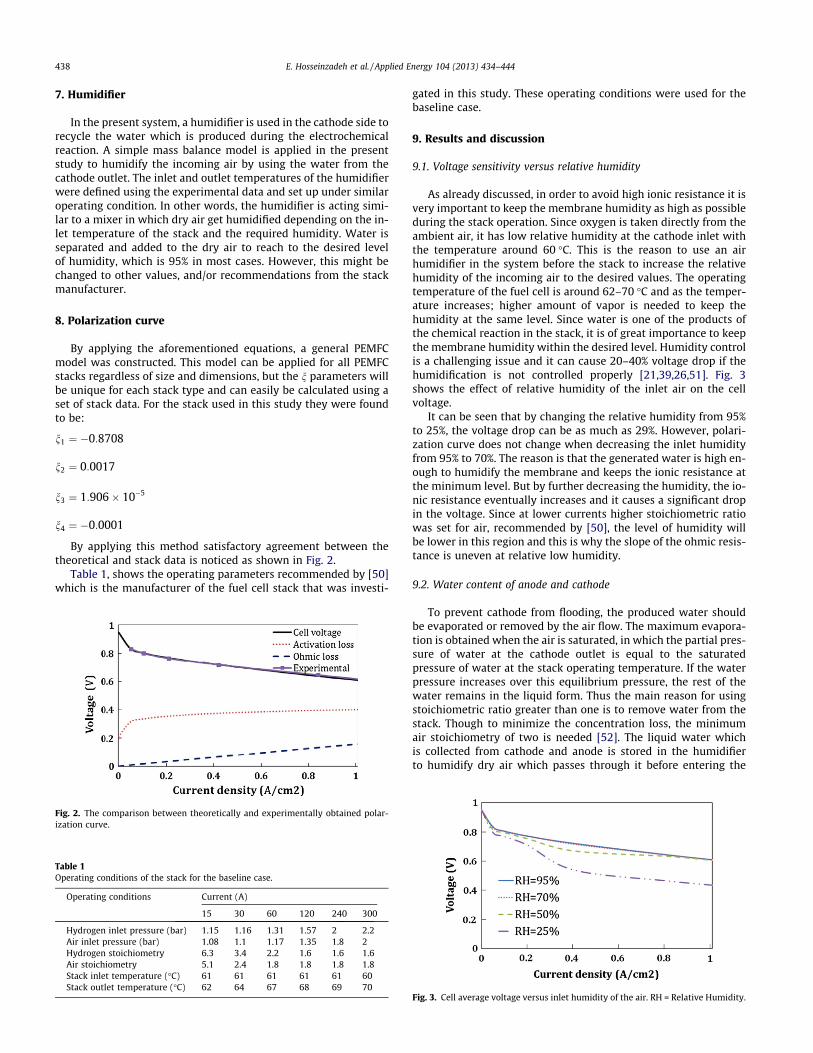
7. Humidifier

In the present system, a humidifier is used in the cathode side torecycle the water which is produced during the electrochemicalreaction. A simple mass balance model is applied in the presentstudy to humidify the incoming air by using the water from thecathode outlet. The inlet and outlet temperatures of the humidifierwere defined using the experimental data and set up under similaroperating condition. In other words, the humidifier is acting simi-lar to a mixer in which dry air get humidified depending on the in-let temperature of the stack and the required humidity. Water isseparated and added to the dry air to reach to the desired levelof humidity, which is 95% in most cases. However, this might bechanged to other values, and/or recommendations from the stackmanufacturer.

8. Polarization curve

By applying the aforementioned equations, a general PEMFCmodel was constructed. This model can be applied for all PEMFCstacks regardless of size and dimensions, but the n parameters willbe unique for each stack type and can easily be calculated using aset of stack data. For the stack used in this study they were foundto be:

n1 ¼ 0:8708

n2 ¼ 0:0017

n3 ¼ 1:906 105

n4 ¼ 0:0001

By applying this method satisfactory agreement between thetheoretical and stack data is noticed as shown in Fig. 2.

Table 1, shows the operating parameters recommended by [50]which is the manufacturer of the fuel cell stack that was investi-

gated in this study. These operating conditions were used for thebaseline case.

9. Results and discussion

9.1. Voltage sensitivity versus relative humidity

As already discussed, in order to avoid high ionic resistance it isvery important to keep the membrane humidity as high as possibleduring the stack operation. Since oxygen is taken directly from theambient air, it has low relative humidity at the cathode inlet withthe temperature around 60 C. This is the reason to use an airhumidifier in the system before the stack to increase the relativehumidity of the incoming air to the desired values. The operatingtemperature of the fuel cell is around 62–70 C and as the temper-ature increases; higher amount of vapor is needed to keep thehumidity at the same level. Since water is one of the products ofthe chemical reaction in the stack, it is of great importance to keepthe membrane humidity within the desired level. Humidity controlis a challenging issue and it can cause 20–40% voltage drop if thehumidification is not controlled properly [21,39,26,51]. Fig. 3shows the effect of relative humidity of the inlet air on the cellvoltage.

It can be seen that by changing the relative humidity from 95%to 25%, the voltage drop can be as much as 29%. However, polari-zation curve does not change when decreasing the inlet humidityfrom 95% to 70%. The reason is that the generated water is high en-ough to humidify the membrane and keeps the ionic resistance atthe minimum level. But by further decreasing the humidity, the io-nic resistance eventually increases and it causes a significant dropin the voltage. Since at lower currents higher stoichiometric ratiowas set for air, recommended by [50], the level of humidity willbe lower in this region and this is why the slope of the ohmic resis-tance is uneven at relative low humidity.

9.2. Water content of anode and cathode

To prevent cathode from flooding, the produced water shouldbe evaporated or removed by the air flow. The maximum evapora-tion is obtained when the air is saturated, in which the partial pres-sure of water at the cathode outlet is equal to the saturatedpressure of water at the stack operating temperature. If the waterpressure increases over this equilibrium pressure, the rest of thewater remains in the liquid form. Thus the main reason for usingstoichiometric ratio greater than one is to remove water from thestack. Though to minimize the concentration loss, the minimumair stoichiometry of two is needed [52]. The liquid water whichis collected from cathode and anode is stored in the humidifierto humidify dry air which passes through it before entering the

Fig. 2. The comparison between theoretically and experimentally obtained polar-ization curve.

Table 1Operating conditions of the stack for the baseline case.

Operating conditions Current (A)

15 30 60 120 240 300

Hydrogen inlet pressure (bar) 1.15 1.16 1.31 1.57 2 2.2Air inlet pressure (bar) 1.08 1.1 1.17 1.35 1.8 2Hydrogen stoichiometry 6.3 3.4 2.2 1.6 1.6 1.6Air stoichiometry 5.1 2.4 1.8 1.8 1.8 1.8Stack inlet temperature (C) 61 61 61 61 61 60Stack outlet temperature (C) 62 64 67 68 69 70

Fig. 3. Cell average voltage versus inlet humidity of the air. RH = Relative Humidity.

438 E. Hosseinzadeh et al. / Applied Energy 104 (2013) 434–444

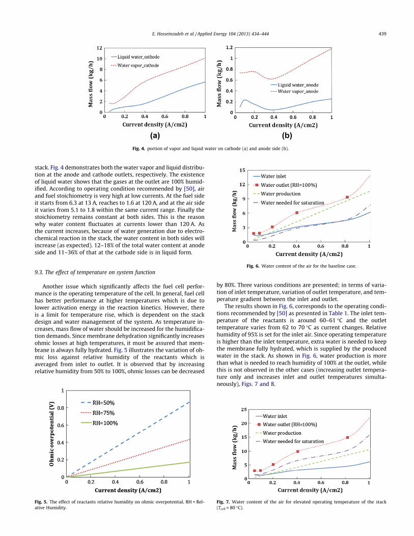
stack. Fig. 4 demonstrates both the water vapor and liquid distribu-tion at the anode and cathode outlets, respectively. The existenceof liquid water shows that the gases at the outlet are 100% humid-ified. According to operating condition recommended by [50], airand fuel stoichiometry is very high at low currents. At the fuel sideit starts from 6.3 at 13 A, reaches to 1.6 at 120 A, and at the air sideit varies from 5.1 to 1.8 within the same current range. Finally thestoichiometry remains constant at both sides. This is the reasonwhy water content fluctuates at currents lower than 120 A. Asthe current increases, because of water generation due to electro-chemical reaction in the stack, the water content in both sides willincrease (as expected). 12–18% of the total water content at anodeside and 11–36% of that at the cathode side is in liquid form.

9.3. The effect of temperature on system function

Another issue which significantly affects the fuel cell perfor-mance is the operating temperature of the cell. In general, fuel cellhas better performance at higher temperatures which is due tolower activation energy in the reaction kinetics. However, thereis a limit for temperature rise, which is dependent on the stackdesign and water management of the system. As temperature in-creases, mass flow of water should be increased for the humidifica-tion demands. Since membrane dehydration significantly increasesohmic losses at high temperatures, it must be assured that mem-brane is always fully hydrated. Fig. 5 illustrates the variation of oh-mic loss against relative humidity of the reactants which isaveraged from inlet to outlet. It is observed that by increasingrelative humidity from 50% to 100%, ohmic losses can be decreased

by 80%. Three various conditions are presented; in terms of varia-tion of inlet temperature, variation of outlet temperature, and tem-perature gradient between the inlet and outlet.

The results shown in Fig. 6, corresponds to the operating condi-tions recommended by [50] as presented in Table 1. The inlet tem-perature of the reactants is around 60–61 C and the outlettemperature varies from 62 to 70 C as current changes. Relativehumidity of 95% is set for the inlet air. Since operating temperatureis higher than the inlet temperature, extra water is needed to keepthe membrane fully hydrated, which is supplied by the producedwater in the stack. As shown in Fig. 6, water production is morethan what is needed to reach humidity of 100% at the outlet, whilethis is not observed in the other cases (increasing outlet tempera-ture only and increases inlet and outlet temperatures simulta-neously), Figs. 7 and 8.

Fig. 4. portion of vapor and liquid water on cathode (a) and anode side (b).

Fig. 5. The effect of reactants relative humidity on ohmic overpotential. RH = Rel-ative Humidity.

Fig. 6. Water content of the air for the baseline case.

Fig. 7. Water content of the air for elevated operating temperature of the stack(Tcell = 80 C).

E. Hosseinzadeh et al. / Applied Energy 104 (2013) 434–444 439

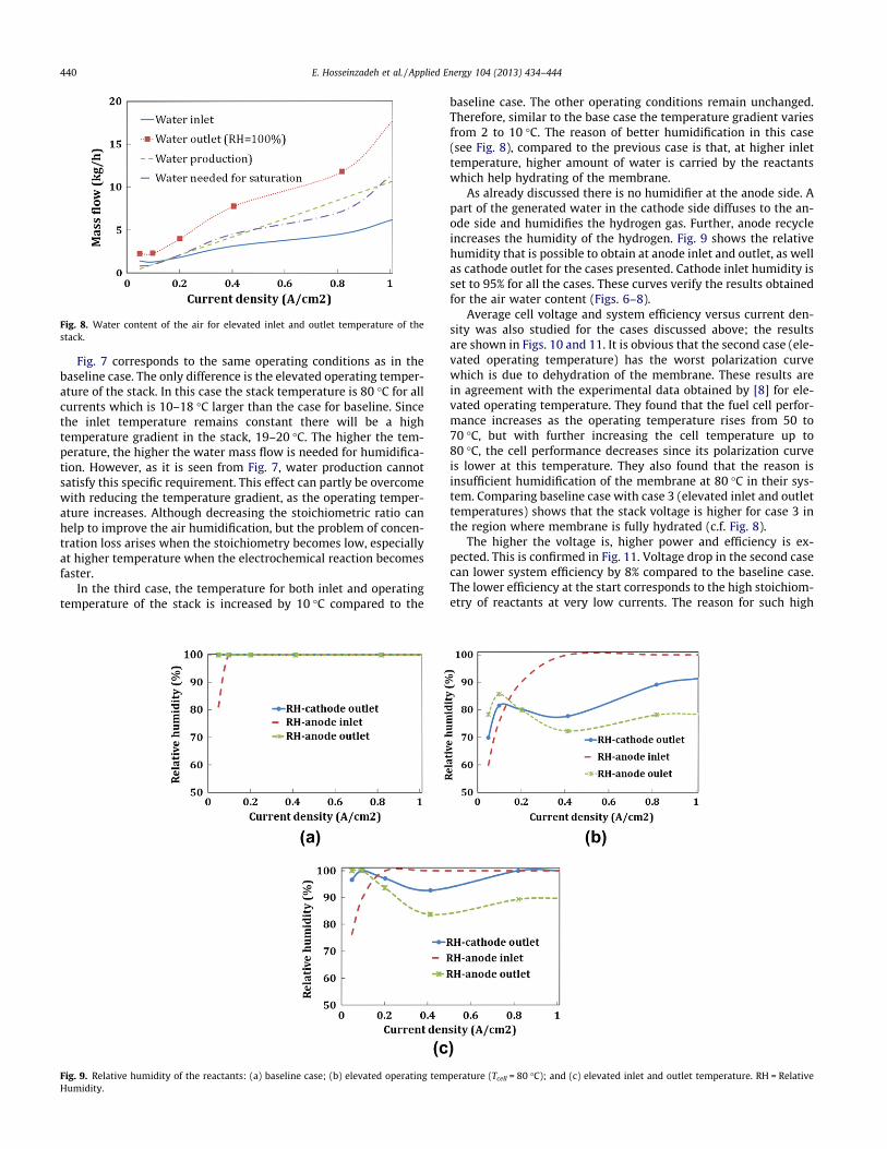
Fig. 7 corresponds to the same operating conditions as in thebaseline case. The only difference is the elevated operating temper-ature of the stack. In this case the stack temperature is 80 C for allcurrents which is 10–18 C larger than the case for baseline. Sincethe inlet temperature remains constant there will be a hightemperature gradient in the stack, 19–20 C. The higher the tem-perature, the higher the water mass flow is needed for humidifica-tion. However, as it is seen from Fig. 7, water production cannotsatisfy this specific requirement. This effect can partly be overcomewith reducing the temperature gradient, as the operating temper-ature increases. Although decreasing the stoichiometric ratio canhelp to improve the air humidification, but the problem of concen-tration loss arises when the stoichiometry becomes low, especiallyat higher temperature when the electrochemical reaction becomesfaster.

In the third case, the temperature for both inlet and operatingtemperature of the stack is increased by 10 C compared to the

baseline case. The other operating conditions remain unchanged.Therefore, similar to the base case the temperature gradient variesfrom 2 to 10 C. The reason of better humidification in this case(see Fig. 8), compared to the previous case is that, at higher inlettemperature, higher amount of water is carried by the reactantswhich help hydrating of the membrane.

As already discussed there is no humidifier at the anode side. Apart of the generated water in the cathode side diffuses to the an-ode side and humidifies the hydrogen gas. Further, anode recycleincreases the humidity of the hydrogen. Fig. 9 shows the relativehumidity that is possible to obtain at anode inlet and outlet, as wellas cathode outlet for the cases presented. Cathode inlet humidity isset to 95% for all the cases. These curves verify the results obtainedfor the air water content (Figs. 6–8).

Average cell voltage and system efficiency versus current den-sity was also studied for the cases discussed above; the resultsare shown in Figs. 10 and 11. It is obvious that the second case (ele-vated operating temperature) has the worst polarization curvewhich is due to dehydration of the membrane. These results arein agreement with the experimental data obtained by [8] for ele-vated operating temperature. They found that the fuel cell perfor-mance increases as the operating temperature rises from 50 to70 C, but with further increasing the cell temperature up to80 C, the cell performance decreases since its polarization curveis lower at this temperature. They also found that the reason isinsufficient humidification of the membrane at 80 C in their sys-tem. Comparing baseline case with case 3 (elevated inlet and outlettemperatures) shows that the stack voltage is higher for case 3 inthe region where membrane is fully hydrated (c.f. Fig. 8).

The higher the voltage is, higher power and efficiency is ex-pected. This is confirmed in Fig. 11. Voltage drop in the second casecan lower system efficiency by 8% compared to the baseline case.The lower efficiency at the start corresponds to the high stoichiom-etry of reactants at very low currents. The reason for such high

Fig. 8. Water content of the air for elevated inlet and outlet temperature of thestack.

Fig. 9. Relative humidity of the reactants: (a) baseline case; (b) elevated operating temperature (Tcell = 80 C); and (c) elevated inlet and outlet temperature. RH = RelativeHumidity.

440 E. Hosseinzadeh et al. / Applied Energy 104 (2013) 434–444

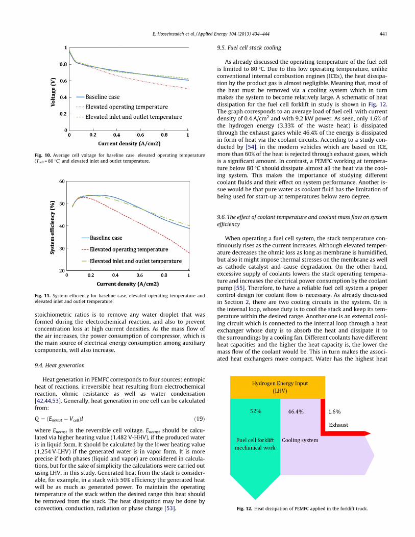
stoichiometric ratios is to remove any water droplet that wasformed during the electrochemical reaction, and also to preventconcentration loss at high current densities. As the mass flow ofthe air increases, the power consumption of compressor, which isthe main source of electrical energy consumption among auxiliarycomponents, will also increase.

9.4. Heat generation

Heat generation in PEMFC corresponds to four sources: entropicheat of reactions, irreversible heat resulting from electrochemicalreaction, ohmic resistance as well as water condensation[42,44,53]. Generally, heat generation in one cell can be calculatedfrom:

Q ¼ ðEnernst VcellÞI ð19Þ

where Enernst is the reversible cell voltage. Enernst should be calcu-lated via higher heating value (1.482 V-HHV), if the produced wateris in liquid form. It should be calculated by the lower heating value(1.254 V-LHV) if the generated water is in vapor form. It is moreprecise if both phases (liquid and vapor) are considered in calcula-tions, but for the sake of simplicity the calculations were carried outusing LHV, in this study. Generated heat from the stack is consider-able, for example, in a stack with 50% efficiency the generated heatwill be as much as generated power. To maintain the operatingtemperature of the stack within the desired range this heat shouldbe removed from the stack. The heat dissipation may be done byconvection, conduction, radiation or phase change [53].

9.5. Fuel cell stack cooling

As already discussed the operating temperature of the fuel cellis limited to 80 C. Due to this low operating temperature, unlikeconventional internal combustion engines (ICEs), the heat dissipa-tion by the product gas is almost negligible. Meaning that, most ofthe heat must be removed via a cooling system which in turnmakes the system to become relatively large. A schematic of heatdissipation for the fuel cell forklift in study is shown in Fig. 12.The graph corresponds to an average load of fuel cell, with currentdensity of 0.4 A/cm2 and with 9.2 kW power. As seen, only 1.6% ofthe hydrogen energy (3.33% of the waste heat) is dissipatedthrough the exhaust gases while 46.4% of the energy is dissipatedin form of heat via the coolant circuits. According to a study con-ducted by [54], in the modern vehicles which are based on ICE,more than 60% of the heat is rejected through exhaust gases, whichis a significant amount. In contrast, a PEMFC working at tempera-ture below 80 C should dissipate almost all the heat via the cool-ing system. This makes the importance of studying differentcoolant fluids and their effect on system performance. Another is-sue would be that pure water as coolant fluid has the limitation ofbeing used for start-up at temperatures below zero degree.

9.6. The effect of coolant temperature and coolant mass flow on systemefficiency

When operating a fuel cell system, the stack temperature con-tinuously rises as the current increases. Although elevated temper-ature decreases the ohmic loss as long as membrane is humidified,but also it might impose thermal stresses on the membrane as wellas cathode catalyst and cause degradation. On the other hand,excessive supply of coolants lowers the stack operating tempera-ture and increases the electrical power consumption by the coolantpump [55]. Therefore, to have a reliable fuel cell system a propercontrol design for coolant flow is necessary. As already discussedin Section 2, there are two cooling circuits in the system. On isthe internal loop, whose duty is to cool the stack and keep its tem-perature within the desired range. Another one is an external cool-ing circuit which is connected to the internal loop through a heatexchanger whose duty is to absorb the heat and dissipate it tothe surroundings by a cooling fan. Different coolants have differentheat capacities and the higher the heat capacity is, the lower themass flow of the coolant would be. This in turn makes the associ-ated heat exchangers more compact. Water has the highest heat

Fig. 10. Average cell voltage for baseline case, elevated operating temperature(Tcell = 80 C) and elevated inlet and outlet temperature.

Fig. 11. System efficiency for baseline case, elevated operating temperature andelevated inlet and outlet temperature.

Fig. 12. Heat dissipation of PEMFC applied in the forklift truck.

E. Hosseinzadeh et al. / Applied Energy 104 (2013) 434–444 441

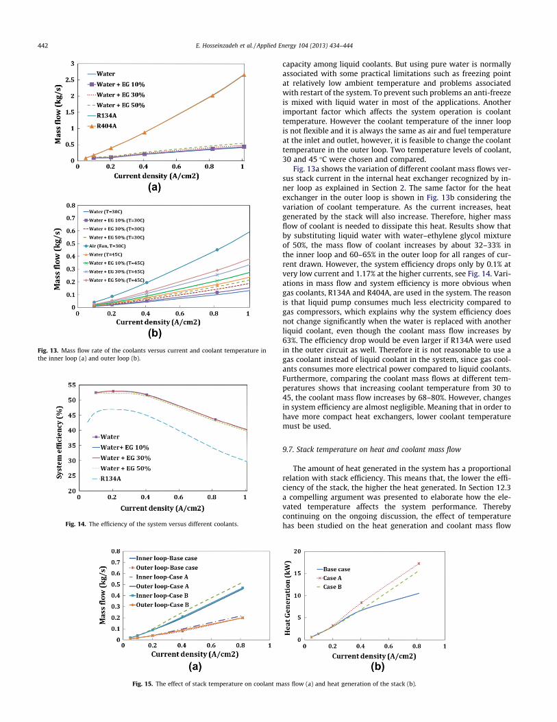
capacity among liquid coolants. But using pure water is normallyassociated with some practical limitations such as freezing pointat relatively low ambient temperature and problems associatedwith restart of the system. To prevent such problems an anti-freezeis mixed with liquid water in most of the applications. Anotherimportant factor which affects the system operation is coolanttemperature. However the coolant temperature of the inner loopis not flexible and it is always the same as air and fuel temperatureat the inlet and outlet, however, it is feasible to change the coolanttemperature in the outer loop. Two temperature levels of coolant,30 and 45 C were chosen and compared.

Fig. 13a shows the variation of different coolant mass flows ver-sus stack current in the internal heat exchanger recognized by in-ner loop as explained in Section 2. The same factor for the heatexchanger in the outer loop is shown in Fig. 13b considering thevariation of coolant temperature. As the current increases, heatgenerated by the stack will also increase. Therefore, higher massflow of coolant is needed to dissipate this heat. Results show thatby substituting liquid water with water–ethylene glycol mixtureof 50%, the mass flow of coolant increases by about 32–33% inthe inner loop and 60–65% in the outer loop for all ranges of cur-rent drawn. However, the system efficiency drops only by 0.1% atvery low current and 1.17% at the higher currents, see Fig. 14. Vari-ations in mass flow and system efficiency is more obvious whengas coolants, R134A and R404A, are used in the system. The reasonis that liquid pump consumes much less electricity compared togas compressors, which explains why the system efficiency doesnot change significantly when the water is replaced with anotherliquid coolant, even though the coolant mass flow increases by63%. The efficiency drop would be even larger if R134A were usedin the outer circuit as well. Therefore it is not reasonable to use agas coolant instead of liquid coolant in the system, since gas cool-ants consumes more electrical power compared to liquid coolants.Furthermore, comparing the coolant mass flows at different tem-peratures shows that increasing coolant temperature from 30 to45, the coolant mass flow increases by 68–80%. However, changesin system efficiency are almost negligible. Meaning that in order tohave more compact heat exchangers, lower coolant temperaturemust be used.

9.7. Stack temperature on heat and coolant mass flow

The amount of heat generated in the system has a proportionalrelation with stack efficiency. This means that, the lower the effi-ciency of the stack, the higher the heat generated. In Section 12.3a compelling argument was presented to elaborate how the ele-vated temperature affects the system performance. Therebycontinuing on the ongoing discussion, the effect of temperaturehas been studied on the heat generation and coolant mass flow

Fig. 13. Mass flow rate of the coolants versus current and coolant temperature inthe inner loop (a) and outer loop (b).

Fig. 14. The efficiency of the system versus different coolants.

Fig. 15. The effect of stack temperature on coolant mass flow (a) and heat generation of the stack (b).

442 E. Hosseinzadeh et al. / Applied Energy 104 (2013) 434–444

of the system, see Fig. 15. For the base case the operating condi-tions recommended by [50] has been used, case A is the same asbaseline case but with increased operating temperature to 80 Cand case B represents the results for the same stack but with ele-vated inlet and outlet temperatures. High heat generation at highertemperature is due to the increased ohmic loss as already dis-cussed which corresponds to a higher coolant demand for the sys-tem. However, the opposite would be observed if the membranewas fully hydrated at high temperature, for example by waterinjection to the membrane. The reason is that for constant amountof heat, larger temperature gradient of the coolant can lead to amore compact heat exchanger; though in that case the size ofthe radiator will increase.

10. Conclusion

A general steady-state model for PEMFC was developed and val-idated against the stack data. The model takes into account theeffects of pressure losses, water crossovers, humidity aspects andvoltage over-potentials in the cells. Water and thermal manage-ment of the stack as well as BOP were investigated in this study.The summary of the results are presented as follows.

For the baseline case 12–18% of the total water content at anodeoutlet and 11–36% of that at the cathode outlet is in liquid formwhich confirms the proper humidification of the system. Variationsin humidity level of inlet air from 25% to 95%, the voltage may dropby 29%. However polarization curve does not change whiledecreasing the inlet humidity from 95% to 70%.

Another issue which significantly affects the fuel cell perfor-mance is the operating temperature of the cell. By increasing thestack temperature to 80 C for all the currents drawn and keepingthe inlet temperatures unchanged, system efficiency decreases by8% compared to the baseline case. Higher the temperature, Higherthe mass flow is needed for humidification and water productioncannot meet this requirement. This effect can be partly improvedby reducing the temperature gradient as the operating tempera-ture increases.

By substituting liquid water with water–ethylene glycol mix-ture of 50%, the mass flow of coolant increases with about 32–33% in the inner loop and 60–65% in the outer loop for all rangesof current. However, the system efficiency drops from 0.1% at verylow current to 1.17% at the highest current studied here (300 A,1 A/cm2). The variation in mass flow and efficiency is more signif-icant when the gas coolants, R134A and R404A, are used in the sys-tem. Therefore, it is not reasonable to use gas coolants in thesystem because they consume most of the electrical power andthereby reduce system efficiencies considerably. Finally, compar-ing of coolant mass flows at different temperatures show that byincreasing coolant temperature from 30 to 45 C, mass flow in-creases by 68–80%. Meaning that to have more compact heatexchangers, then lower temperature for the coolant is advanta-geous. However, the efficiency differences will be negligible.

Acknowledgements

The authors would like to thank The Danish National AdvancedTechnology Foundation (Højteknologifonden) for financial supportof this project and H2Logic company for their technical support.

References

[1] Kazim A. Introduction of PEM fuel-cell vehicles in the transportation sector ofthe United Arab Emirates. J Appl Energy 2003;74:125–33.

[2] Contreras A, Posso F, Guervos E. Modelling and simulation of the utilization ofa PEM fuel cell in the rural sector of Venezuela. J Appl Energy2010;87:1376–85.

[3] Tang Y, Yuan W, Pan M, Wan Z. Experimental investigation on the dynamicperformance of a hybrid PEM fuel cell/battery system for lightweight electricvehicle application. J Appl Energy 2011;88:68–76.

[4] Alaefour I, Karimi G, Jiao K, Li X. Measurement of current distribution in aproton exchange membrane fuel cell with various flow arrangements – aparametric study. J Appl Energy 2012;93:80–9.

[5] Wang Y, Chen KS, Mishler J, Chan Cho S, Cordobes Adroher X. A review ofpolymer electrolyte membrane fuel cells: technology, applications, and needson fundamental research. J Appl Energy 2011;88:981–1007.

[6] Wang Y, Al Shakhshir S, Li X. Development and impact of sandwich wettabilitystructure for gas distribution media on PEM fuel cell performance. J ApplEnergy 2011;2011(88):2168–75.

[7] Madhusudana Rao R, Rengaswamy R. Optimization study of an agglomeratemodel for platinum reduction and performance in PEM fuel cell cathode. JChem Eng Res Des 2006;84:952–64.

[8] Yim S-D, Lee W-Y, Yoon Y-G, Sohn Y-J, Park G-G, Yang T-H, et al. Optimizationof bifunctional electrocatalyst for PEM unitized regenerative fuel cell. JElectrochim Acta 2004;50:713–8.

[9] Wu J, Yuan XZ, Martin JJ, Wang H, Zhang J, Shen J, et al. A review of PEM fuelcell durability: degradation mechanisms and mitigation strategies. J PowerSources 2008;184:104–19.

[10] Iyuke SE, Mohamad AB, Kadhum AAH, Daud WRW, Rachid C. Improvedmembrane and electrode assemblies for proton exchange membrane fuel cells.J Power Sources 2003;114:195–202.

[11] Ang SMC, Brett DJ, Fraga ES. A multi-objective optimisation model for a generalpolymer electrolyte membrane fuel cell system. J Power Sources2010;195:2754–63.

[12] Wu H-W, Ku H-W. The optimal parameters estimation for rectangularcylinders installed transversely in the flow channel of PEMFC from a three-dimensional PEMFC model and the Taguchi method. J Appl Energy2011;88:4879–90.

[13] Meidanshahi V, Karimi G. Dynamic modeling, optimization and control ofpower density in a PEM fuel cell. J Appl Energy 2012;93:98–105.

[14] Yan W-M, Wang X-D, Lee D-J, Zhang X-X, Guo Y-F, Su A. Experimental study ofcommercial size proton exchange membrane fuel cell performance. J ApplEnergy 2011;88:392–6.

[15] Tang Y, Yuan W, Pan M, Li Z, Chen G, Li Y. Experimental investigation ofdynamic performance and transient responses of a kW-class PEM fuel cellstack under various load changes. J Appl Energy 2010;87:1410–7.

[16] Nolan J, Kolodziej J. Modeling of an automotive fuel cell thermal system. JPower Sources 2010;195:4743–52.

[17] Ang SMC, Brett DJL, Fraga ES. A multi-objective optimisation model for ageneral polymer electrolyte membrane fuel cell system. J Power Sources2010;195:2754–63.

[18] Zhang G, Kandlikar SG. A critical review of cooling techniques in protonexchange membrane fuel cell stacks. Int J Hydrogen Energy 2012;37:2412–29.

[19] Zhang J, Xie Z, Zhang J, Tang Y, Song C, Navessin T, et al. High temperature PEMfuel cells. J Power Sources 2006;160:872–91.

[20] Kandlikar SG, Lu Z. Thermal management issues in a PEMFC stack – a briefreview of current status. J Appl Therm Eng 2009;29:1276–80.

[21] Anderson R, Blanco M, Bi X, Wilkinson DP. Anode water removal and cathodegas diffusion layer flooding in a proton exchange membrane fuel cell. Int JHydrogen Energy 2012;37:6093–103.

[22] Nguyen TV, Knobbe MW. A liquid water management strategy for PEM fuelcell stacks. J Power Sources 2003;114:70–9.

[23] Picot D, Metkemeijer R, Bezian JJ, Rouveyre L. Impact of the water symmetryfactor on humidification and coolallengesing strategies for PEM fuel cellstacks. J Power Sources 1998;75:251–60.

[24] Jiao K, Li X. Water transport in polymer electrolyte membrane fuel cells. J ProgEnergy Combust Sci 2011;37:221–91.

[25] Gerteisen D, Heilmann T, Ziegler C. Modeling the phenomena of dehydrationand flooding of a polymer electrolyte membrane fuel cell. J Power Sources2009;187:165–81.

[26] Buchi F, Srinivasan S. Operating proton exchange membrane fuel cells withoutexternal humidification of the reactant gases. J Electrochem Soc1997;144:2767–72.

[27] Shah A, Kim G-S, Gervais W, Young A, Promislow K, Li J, et al. The effects ofwater and microstructure on the performance of polymer electrolyte fuel cells.J Power Sources 2006;160:1251–68.

[28] Shao Y, Yin G, Wang Z, Gao Y. Proton exchange membrane fuel cell from lowtemperature to high temperature: material challenges. J Power Sources2007;167:235–42.

[29] Juhl Andreasen S, Rabjerg Vang J, Knudsen Kær S. High temperature PEM fuelcell performance characterisation with CO and CO2 using electrochemicalimpedance spectroscopy. Int J Hydrogen Energy 2011;36:9815–30.

[30] Faghri A, Guo Z. Challenges and opportunities of thermal management issuesrelated to fuel cell technology and modeling. Int J Heat Mass Transfer2005;48:3891–920.

[31] Jung C-Y, Shim H-S, Koo S-M, Lee S-H, Yi S-C. Investigations of the temperaturedistribution in proton exchange membrane fuel cells. J Appl Energy2012;93:733–41.

[32] Elmegaard B, Houbak N. DNA – a general energy system simulation tool. In:Proceeding of SIMS, Trondheim, Norway; 2005.

[33] Santarelli M, Torchio M, Cochis P. Parameters estimation of a PEM fuel cellpolarization curve and analysis of their behavior with temperature. J PowerSources 2006;159:824–35.

E. Hosseinzadeh et al. / Applied Energy 104 (2013) 434–444 443

[34] Amphlett JC, Baumert RM, Mann RF, Peppley BA, Roberge PR. Performancemodeling of the Ballard Mark IV solid polymer electrolyte fuel cell II: empiricalmodel development. J Electrochem Soc 1995;142:9–15.

[35] Mann RF, Amphlett JC, Hooper MAI, Jensen HM, Peppley BA, Roberge PR.Development and application of a generalised steady-state electrochemicalmodel for a PEM fuel cell. J Power Sources 2000;86:173–80.

[36] Candusso D, Harel F, De Bernardinis A, François X, Péra M, Hissel D, et al.Characterisation and modelling of a 5 kW PEMFC for transportationapplications. Int J Hydrogen Energy 2006;31:1019–30.

[37] Mammar K, Chaker A. Modelling and fuzzy logic control of PEM fuel cellsystem power generation for residential application. J Electr Electron Eng2009;9:1073–81.

[38] Santarelli M, Torchio M. Experimental analysis of the effects of the operatingvariables on the performance of a single PEMFC. J Energy Convers Manage2007;48:40–51.

[39] Zhang L, Pan M, Quan S. Model predictive control of water management inPEMFC. J Power Sources 2008;180:322–9.

[40] Spiegel CS. Designing & building fuel cells. 1st ed., New York; 2007.[41] Springer TE, Zawodzinski TA, Gottesfeld S. Polymer electrolyte fuel cell model.

J Electrochem Soc 1991;138:2334–42.[42] Martins L, Gardolinski J, Vargas J, Ordonez J, Amico S, Forte M.

The experimental validation of a simplified PEMFC simulation modelfor design and optimization purposes. J Appl Therm Eng 2009;29:3036–48.

[43] Gurau V, Barbir F, Liu H. An analytical solution of a half-cell model for PEM fuelcells. J Electrochem Soc 2000;147:2468–77.

[44] Spinelli P, Francia C, Ambrosio E, Lucariello M. Semi-empirical evaluation ofPEMFC electro-catalytic activity. J Power Sources 2008;178:517–24.

[45] Haji S. Analytical modeling of PEM fuel cell I–V curve. J Renew Energy2011;36:451–8.

[46] Al-Dabbagh AW, Lu L, Mazza A. Modelling, simulation and control of a protonexchange membrane fuel cell (PEMFC) power system. Int J Hydrogen Energy2010;35:5061–9.

[47] Pei P, Yang W, Li P. Numerical prediction on an automotive fuel cell drivingsystem. Int J Hydrogen Energy 2005;31:361–9.

[48] Murahashi T, Naiki M, Nishiyama E. Water transport in the proton exchange-membrane fuel cell: comparison of model computation and measurements ofeffective drag. J Power Sources 2006;162:1130–6.

[49] Shimpalee S, Dutta S. Numerical prediction of temperature distribution in PEMfuel cells. J Numerical Heat Transfer 2000;38:111–28.

[50] Mark9 SSL™ of Ballard Company, Product manual and integration guide; 2008.[51] Tsushima S, Hirai S. In situ diagnostics for water transport in proton exchange

membrane fuel cells. J Prog Energy Combust Sci 2011;37:204–20.[52] Larminie J, Dicks A. Fuel cell systems explained. 2nd ed. West Sussex: Wiley;

2000.[53] Sasmito AP, Birgersson E, Mujumdar AS. Numerical investigation of liquid

water cooling for a proton exchange membrane fuel cell stack. J Heat TransferEng 2011;32:151–67.

[54] Frank G. Prospects and requirements of high temperature PEMFC. In:Proceedings of the 2nd European PEFC Forum, Lucerne, Switzerland; 2003.

[55] Woo Ahn J, Yul Choe S. Coolant controls of a PEM fuel cell system. J PowerSources 2008;2008(179):252–64.

444 E. Hosseinzadeh et al. / Applied Energy 104 (2013) 434–444

Appendix D

Paper III

Performance simulation and analysis of a fuel cell/battery hybrid forklift truck

186

Performance simulation and analysis of a fuel cell/batteryhybrid forklift truck

Elham Hosseinzadeh a, Masoud Rokni a, Suresh G. Advani b, Ajay K. Prasad b,*aDepartment of Mechanical Engineering, Thermal Energy Systems, Technical University of Denmark, 2800 Kgs. Lyngby, DenmarkbCenter for Fuel Cell Research, Department of Mechanical Engineering, University of Delaware, Newark, DE 19716, USA

a r t i c l e i n f o

Article history:

Received 4 December 2012

Received in revised form

22 January 2013

Accepted 24 January 2013

Available online 23 February 2013

Keywords:

Forklift

Hybrid drivetrain

PEM fuel cell

Lead acid battery

Power management system

Drive cycle

a b s t r a c t

The performance of a forklift truck powered by a hybrid system consisting of a PEM fuel cell

and a lead acid battery is modeled and investigated by conducting a parametric study.

Various combinations of fuel cell size and battery capacity are employed in conjunction

with two distinct control strategies to study their effect on hydrogen consumption and

battery state-of-charge for two drive cycles characterized by different operating speeds and

forklift loads. The results show that for all case studies, the combination of a 110 cell stack

with two strings of 55 Ah batteries is the most economical choice for the hybrid system

based on system size and hydrogen consumption. In addition, it is observed that hydrogen

consumption decreases by about 24% when the maximum speed of the drive cycle is

decreased from 4.5 to 3 m/s. Similarly, by decreasing the forklift load from 2.5 to 1.5 ton, the

hydrogen consumption decreases by over 20%.

Copyright ª 2013, Hydrogen Energy Publications, LLC. Published by Elsevier Ltd. All rights

reserved.

1. Introduction

Proton exchange membrane (PEM) fuel cells are considered

good candidates for automotive applications due to their low

operating temperatures and high power density. However,

fuel cell systems face significant barriers to commercializa-

tion owing to high cost and inadequate lifetime. PEM fuel cell

durability is principally compromised by the degradation of

the membrane electrode assembly during long-term oper-

ation [1]. Fuel cells can be implemented in automotive pow-

ertrains either as standalone systems or in combination with

other power sources such as a battery or an ultracapacitor to

create a hybrid system. Such hybrid systems exhibit distinct

advantages such as the ability to downsize the stack which in

turn decreases the fuel cell cost, and also isolating the fuel

cell from load fluctuations which promotes stack lifetime.

In addition, hybridization can improve fuel economy by

exploiting regenerative power from the traction motor while

braking. Such hybrid powertrains are particularly well suited

for transit applications where the average power demand is

low due to frequent starts and stops of the vehicle [2].

The fuel economy of a hybrid vehicle is determined by

the overall size and weight of the vehicle, design of the hybrid

platform, energy management strategy, driving conditions,

etc. [3]. According to [4] an advanced control strategy is

necessary to achieve high fuel economy and good drivability.

The challenges associated with dynamic operating conditions

in automotive applications [5] emphasize the importance of

an optimal control strategy. The literature reveals that previ-

ous efforts have focused either on the design and modeling of

* Corresponding author. 126 Spencer Lab, Department of Mechanical Engineering, University of Delaware, Newark, DE 19716-3140, USA.Tel.: þ1 302 831 2960.

E-mail address: prasad@udel.edu (A.K. Prasad).

Available online at www.sciencedirect.com

journal homepage: www.elsevier .com/locate/he

i n t e r n a t i o n a l j o u r n a l o f h y d r o g e n en e r g y 3 8 ( 2 0 1 3 ) 4 2 4 1e4 2 4 9

0360-3199/$ e see front matter Copyright ª 2013, Hydrogen Energy Publications, LLC. Published by Elsevier Ltd. All rights reserved.http://dx.doi.org/10.1016/j.ijhydene.2013.01.168

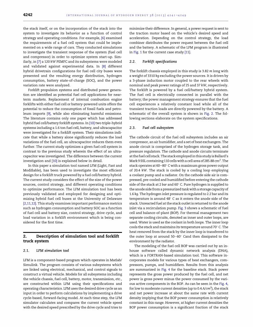
the stack itself, or on the incorporation of the stack into the

system to investigate its behavior as a function of control

strategy and operating conditions. For example, [6] examined

the requirements of a fuel cell system that could be imple-

mented on a wide range of cars. They conducted simulations

to investigate the transient response of the system (fuel cell

and compressor) in order to optimize system start-up. Sim-

ilarly, in [7] a 120 kW PEMFC and its subsystemsweremodeled

and validated against experimental data. In [8] different

hybrid drivetrain configurations for fuel cell city buses were

presented and the resulting energy distribution, hydrogen

consumption, battery state-of-charge (SOC), and the power

variation rate were analyzed.

Forklift propulsion systems and distributed power genera-

tion are identified as potential fuel cell applications for near-

term markets. Replacement of internal combustion engine

forklifts with either fuel cell or battery-powered units offers the

potential to reduce the consumption of fossil fuels and petro-

leum imports [9], while also eliminating harmful emissions.

The literature contains only one paper which has addressed

hybrid fuel cell/battery forklift systems. In [10] two triple-hybrid

systems including a 1.6 ton fuel cell, battery, and ultracapacitor

were investigated for a forklift system. Their simulations indi-

cate that while a battery alone significantly reduces the load

variations of the fuel cell, an ultracapacitor reduces them even

further. The current study optimizes a given fuel cell system in

contrast to the previous study wherein the effect of an ultra-

capacitor was investigated. The difference between the current

investigation and [10] is explained below in detail.

In this paper a simulation tool named LFM (Light, Fast and

Modifiable), has been used to investigate the most efficient

design for a forklift truck powered by a fuel cell/battery hybrid.

The current study considers the effect of the size of the power

sources, control strategy, and different operating conditions

to optimize performance. The LFM simulation tool has been

previously validated and employed for designing and opti-

mizing hybrid fuel cell buses at the University of Delaware

[2,11,12]. This study examines important performancemetrics

such as hydrogen consumption and battery SOC as a function

of fuel cell and battery size, control strategy, drive cycle, and

load variation in a forklift environment which is being con-

sidered for the first time.

2. Description of simulation tool and forklifttruck system

2.1. LFM simulation tool

LFM is a component-based program which operates in Matlab/

Simulink. The program consists of various subsystems which

are linked using electrical, mechanical, and control signals to

construct a virtual vehicle. Models for all subsystems including

the vehicle chassis, fuel cell, battery, motor, transmission, etc.,

are constructed within LFM using their specifications and

operating characteristics. LFMuses the desireddrive cycle as an

input in order to perform calculations by implementing a drive

cycle-based, forward-facing model. At each time step, the LFM

simulator calculates and compares the current vehicle speed

with the desired speed prescribed by the drive cycle and tries to

minimize their difference. In general, a power request is sent to

the traction motor based on the vehicle’s desired speed and

acceleration. Depending on the control strategy, the load

combiner distributes the power request between the fuel cell

and the battery. A schematic of the LFM program is illustrated

in Fig. 1 for the current case study [11].

2.2. Forklift specifications

The forklift chassis employed in this study is 3.82 m long with

a weight of 3310 kg excluding the power sources. It is driven by

a 3-phase induction motor coupled to the rear wheels with

nominal and peak power ratings of 25 and 37 kW, respectively.

The forklift is powered by a fuel cell/battery hybrid system.

The fuel cell is electrically connected in parallel with the

battery; the powermanagement strategy ensures that the fuel

cell experiences a relatively constant load while all of the

transient traction loads are directly powered by the battery. A

schematic of the overall system is shown in Fig. 2. The fol-

lowing sections elaborate on the system specifications.

2.3. Fuel cell subsystem

The cathode circuit of the fuel cell subsystem includes an air

compressor, anair humidifier, anda set of heat exchangers. The

anode circuit is comprised of the hydrogen storage tank, and

pressure regulators. The cathode and anode circuits terminate

at thefuelcell stack.Thestackemployed inthisstudy isBallard’s

Mark9SSLcontaining110cellswithacell areaof285.88cm2.The

stack operates at 60e80 Cwith amaximumgross power output

of 20.4 kW. The stack is cooled by a cooling loop employing

a coolant pump and a radiator. On the cathode side air is com-

pressed, pre-cooled and humidified before entering the cathode

side of the stack at 2 bar and 60 C. Pure hydrogen is supplied to

theanodeside fromapressurizedtankwithastoragecapacityof

1.6 kg. Thehydrogen inlet pressure is regulated to 2.2 bar and its

temperature is around 48 C as it enters the anode side of the

stack. Unreacted fuel at the stack outlet is returned to the anode

inlet via a recirculation pump. Fig. 3 shows a schematic of fuel

cell and balance-of-plant (BOP). For thermal management two

separate cooling circuits, denoted as inner and outer loops, are

used.Water is used as the coolant in both loops. The inner loop

cools the stack andmaintains its temperature around70 C. The

heat removed from the stack by the inner loop is transferred to

the outer loop at around 50e60 Cand then dissipated to the

environment by the radiator.

The modeling of the fuel cell BOP was carried out by an in-

house software called dynamic network analysis (DNA),

which is a FORTRAN-based simulation tool. This software in-

corporates models for various types of heat exchangers, com-

pressors, pumps, and humidifiers. Results from this analysis

are summarized in Fig. 4 for the baseline stack. Stack power

represents the gross power produced by the fuel cell, and net

power is gross power minus the power consumed by the vari-

ous active components in the BOP. As can be seen in the Fig. 4,

for low tomoderate current densities (up to 0.4A/cm2), the stack

and net power increase at about the same rate with current

density implying that the BOP power consumption is relatively

constant in this range. However, at higher current densities the

BOP power consumption is a significant fraction of the stack

i n t e rn a t i o n a l j o u r n a l o f h y d r o g e n en e r g y 3 8 ( 2 0 1 3 ) 4 2 4 1e4 2 4 94242

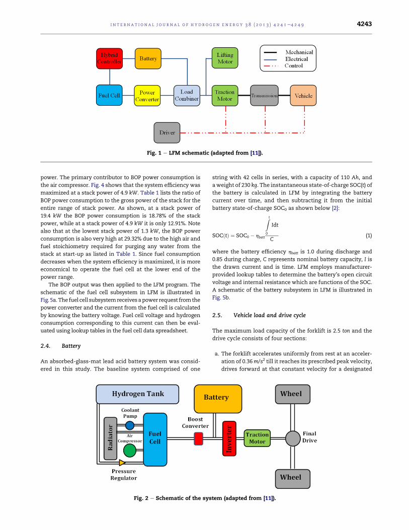
power. The primary contributor to BOP power consumption is

the air compressor. Fig. 4 shows that the system efficiency was

maximized at a stack power of 4.9 kW. Table 1 lists the ratio of

BOP power consumption to the gross power of the stack for the

entire range of stack power. As shown, at a stack power of

19.4 kW the BOP power consumption is 18.78% of the stack

power, while at a stack power of 4.9 kW it is only 12.91%. Note

also that at the lowest stack power of 1.3 kW, the BOP power

consumption is also very high at 29.32% due to the high air and

fuel stoichiometry required for purging any water from the

stack at start-up as listed in Table 1. Since fuel consumption

decreases when the system efficiency is maximized, it is more

economical to operate the fuel cell at the lower end of the

power range.

The BOP output was then applied to the LFM program. The

schematic of the fuel cell subsystem in LFM is illustrated in

Fig. 5a.The fuel cell subsystemreceivesapower request fromthe

power converter and the current from the fuel cell is calculated

by knowing the battery voltage. Fuel cell voltage and hydrogen

consumption corresponding to this current can then be eval-

uated using lookup tables in the fuel cell data spreadsheet.

2.4. Battery

An absorbed-glass-mat lead acid battery system was consid-

ered in this study. The baseline system comprised of one

string with 42 cells in series, with a capacity of 110 Ah, and

aweight of 230 kg. The instantaneous state-of-charge SOC(t) of

the battery is calculated in LFM by integrating the battery

current over time, and then subtracting it from the initial

battery state-of-charge SOC0 as shown below [2]:

SOCðtÞ ¼ SOC0 hbatt

Z t

0

Idt

C(1)

where the battery efficiency hbatt is 1.0 during discharge and

0.85 during charge, C represents nominal battery capacity, I is

the drawn current and is time. LFM employs manufacturer-

provided lookup tables to determine the battery’s open circuit

voltage and internal resistance which are functions of the SOC.

A schematic of the battery subsystem in LFM is illustrated in

Fig. 5b.

2.5. Vehicle load and drive cycle

The maximum load capacity of the forklift is 2.5 ton and the

drive cycle consists of four sections:

a. The forklift accelerates uniformly from rest at an acceler-

ation of 0.36m/s2 till it reaches its prescribed peak velocity,

drives forward at that constant velocity for a designated

Fig. 1 e LFM schematic (adapted from [11]).

Fig. 2 e Schematic of the system (adapted from [11]).

i n t e r n a t i o n a l j o u r n a l o f h y d r o g e n en e r g y 3 8 ( 2 0 1 3 ) 4 2 4 1e4 2 4 9 4243

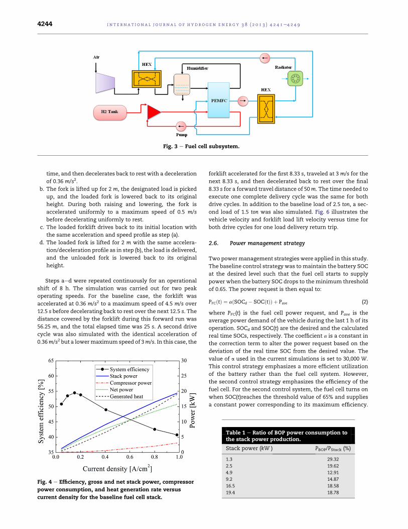
time, and then decelerates back to rest with a deceleration

of 0.36 m/s2.

b. The fork is lifted up for 2 m, the designated load is picked

up, and the loaded fork is lowered back to its original

height. During both raising and lowering, the fork is

accelerated uniformly to a maximum speed of 0.5 m/s

before decelerating uniformly to rest.

c. The loaded forklift drives back to its initial location with

the same acceleration and speed profile as step (a).

d. The loaded fork is lifted for 2 m with the same accelera-

tion/deceleration profile as in step (b), the load is delivered,

and the unloaded fork is lowered back to its original

height.

Steps aed were repeated continuously for an operational

shift of 8 h. The simulation was carried out for two peak

operating speeds. For the baseline case, the forklift was

accelerated at 0.36 m/s2 to a maximum speed of 4.5 m/s over

12.5 s before decelerating back to rest over the next 12.5 s. The

distance covered by the forklift during this forward run was

56.25 m, and the total elapsed time was 25 s. A second drive

cycle was also simulated with the identical acceleration of

0.36m/s2 but a lowermaximum speed of 3m/s. In this case, the

forklift accelerated for the first 8.33 s, traveled at 3 m/s for the

next 8.33 s, and then decelerated back to rest over the final

8.33 s for a forward travel distance of 50m. The time needed to

execute one complete delivery cycle was the same for both

drive cycles. In addition to the baseline load of 2.5 ton, a sec-

ond load of 1.5 ton was also simulated. Fig. 6 illustrates the

vehicle velocity and forklift load lift velocity versus time for

both drive cycles for one load delivery return trip.

2.6. Power management strategy

Two powermanagement strategies were applied in this study.

The baseline control strategy was to maintain the battery SOC

at the desired level such that the fuel cell starts to supply

power when the battery SOC drops to theminimum threshold

of 0.65. The power request is then equal to:

PFCðtÞ ¼ aðSOCd SOCðtÞÞ þ Pave (2)

where PFC(t) is the fuel cell power request, and Pave is the

average power demand of the vehicle during the last 1 h of its

operation. SOCd and SOC(t) are the desired and the calculated

real time SOCs, respectively. The coefficient a is a constant in

the correction term to alter the power request based on the

deviation of the real time SOC from the desired value. The

value of a used in the current simulations is set to 30,000 W.

This control strategy emphasizes a more efficient utilization

of the battery rather than the fuel cell system. However,

the second control strategy emphasizes the efficiency of the

fuel cell. For the second control system, the fuel cell turns on

when SOC(t)reaches the threshold value of 65% and supplies

a constant power corresponding to its maximum efficiency.

Fig. 3 e Fuel cell subsystem.

Fig. 4 e Efficiency, gross and net stack power, compressor

power consumption, and heat generation rate versus

current density for the baseline fuel cell stack.

Table 1 e Ratio of BOP power consumption tothe stack power production.

Stack power (kW ) PBOP/PStack (%)

1.3 29.32

2.5 19.62

4.9 12.91

9.2 14.87

16.5 18.58

19.4 18.78

i n t e rn a t i o n a l j o u r n a l o f h y d r o g e n en e r g y 3 8 ( 2 0 1 3 ) 4 2 4 1e4 2 4 94244

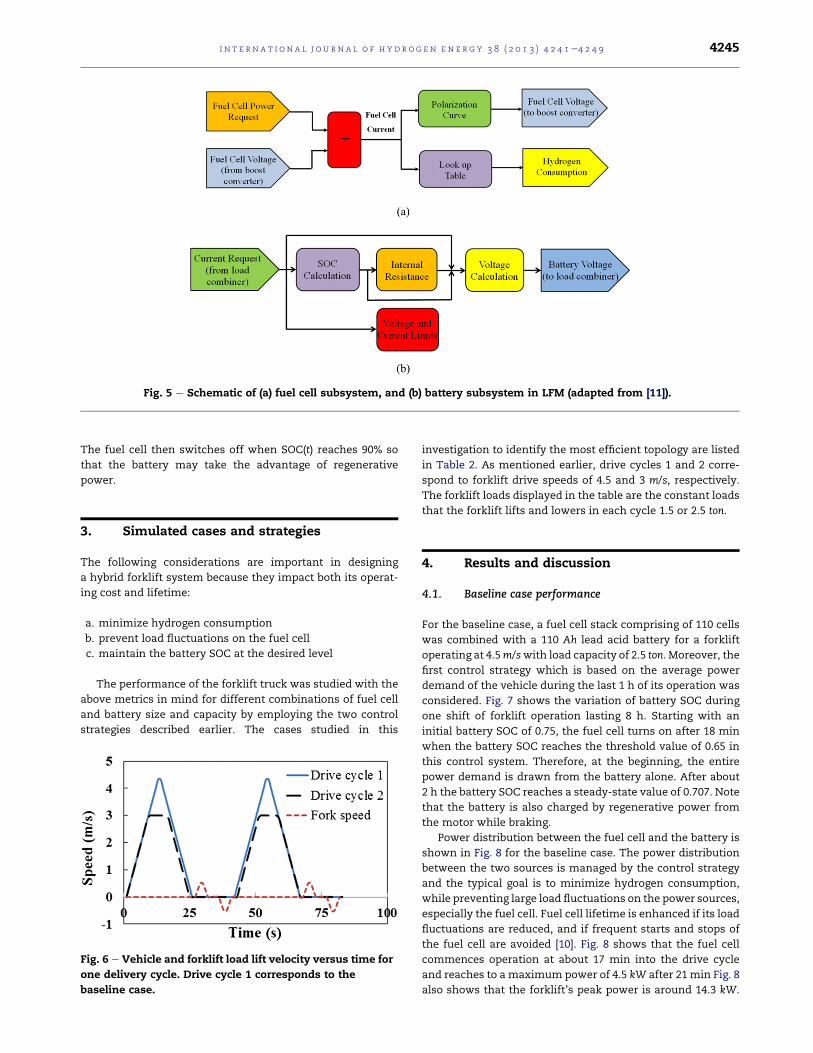
The fuel cell then switches off when SOC(t) reaches 90% so

that the battery may take the advantage of regenerative

power.

3. Simulated cases and strategies

The following considerations are important in designing

a hybrid forklift system because they impact both its operat-

ing cost and lifetime:

a. minimize hydrogen consumption

b. prevent load fluctuations on the fuel cell

c. maintain the battery SOC at the desired level

The performance of the forklift truck was studied with the

above metrics in mind for different combinations of fuel cell

and battery size and capacity by employing the two control

strategies described earlier. The cases studied in this

investigation to identify the most efficient topology are listed

in Table 2. As mentioned earlier, drive cycles 1 and 2 corre-

spond to forklift drive speeds of 4.5 and 3 m/s, respectively.

The forklift loads displayed in the table are the constant loads

that the forklift lifts and lowers in each cycle 1.5 or 2.5 ton.

4. Results and discussion

4.1. Baseline case performance

For the baseline case, a fuel cell stack comprising of 110 cells

was combined with a 110 Ah lead acid battery for a forklift

operating at 4.5m/swith load capacity of 2.5 ton. Moreover, the

first control strategy which is based on the average power

demand of the vehicle during the last 1 h of its operation was

considered. Fig. 7 shows the variation of battery SOC during

one shift of forklift operation lasting 8 h. Starting with an

initial battery SOC of 0.75, the fuel cell turns on after 18 min

when the battery SOC reaches the threshold value of 0.65 in

this control system. Therefore, at the beginning, the entire

power demand is drawn from the battery alone. After about

2 h the battery SOC reaches a steady-state value of 0.707. Note

that the battery is also charged by regenerative power from

the motor while braking.

Power distribution between the fuel cell and the battery is

shown in Fig. 8 for the baseline case. The power distribution

between the two sources is managed by the control strategy

and the typical goal is to minimize hydrogen consumption,

while preventing large load fluctuations on the power sources,

especially the fuel cell. Fuel cell lifetime is enhanced if its load

fluctuations are reduced, and if frequent starts and stops of

the fuel cell are avoided [10]. Fig. 8 shows that the fuel cell

commences operation at about 17 min into the drive cycle

and reaches to a maximum power of 4.5 kW after 21 min Fig. 8

also shows that the forklift’s peak power is around 14.3 kW.

Fig. 5 e Schematic of (a) fuel cell subsystem, and (b) battery subsystem in LFM (adapted from [11]).

Fig. 6 e Vehicle and forklift load lift velocity versus time for

one delivery cycle. Drive cycle 1 corresponds to the

baseline case.

i n t e r n a t i o n a l j o u r n a l o f h y d r o g e n en e r g y 3 8 ( 2 0 1 3 ) 4 2 4 1e4 2 4 9 4245

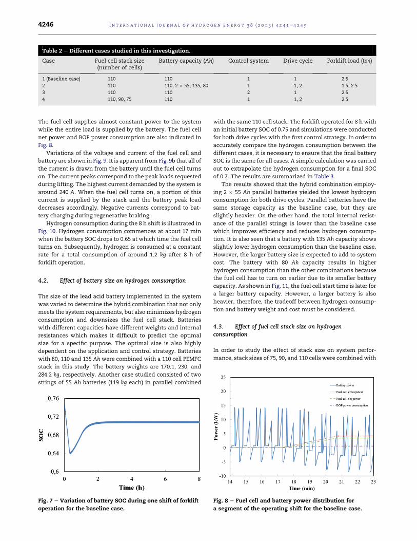
The fuel cell supplies almost constant power to the system

while the entire load is supplied by the battery. The fuel cell

net power and BOP power consumption are also indicated in

Fig. 8.

Variations of the voltage and current of the fuel cell and

battery are shown in Fig. 9. It is apparent from Fig. 9b that all of

the current is drawn from the battery until the fuel cell turns

on. The current peaks correspond to the peak loads requested

during lifting. The highest current demanded by the system is

around 240 A. When the fuel cell turns on, a portion of this

current is supplied by the stack and the battery peak load

decreases accordingly. Negative currents correspond to bat-

tery charging during regenerative braking.

Hydrogen consumption during the 8 h shift is illustrated in

Fig. 10. Hydrogen consumption commences at about 17 min

when the battery SOC drops to 0.65 at which time the fuel cell

turns on. Subsequently, hydrogen is consumed at a constant

rate for a total consumption of around 1.2 kg after 8 h of

forklift operation.

4.2. Effect of battery size on hydrogen consumption

The size of the lead acid battery implemented in the system

was varied to determine the hybrid combination that not only

meets the system requirements, but alsominimizes hydrogen

consumption and downsizes the fuel cell stack. Batteries

with different capacities have different weights and internal

resistances which makes it difficult to predict the optimal

size for a specific purpose. The optimal size is also highly

dependent on the application and control strategy. Batteries

with 80, 110 and 135 Ah were combined with a 110 cell PEMFC

stack in this study. The battery weights are 170.1, 230, and

284.2 kg, respectively. Another case studied consisted of two

strings of 55 Ah batteries (119 kg each) in parallel combined

with the same 110 cell stack. The forklift operated for 8 h with

an initial battery SOC of 0.75 and simulations were conducted

for both drive cycles with the first control strategy. In order to

accurately compare the hydrogen consumption between the

different cases, it is necessary to ensure that the final battery

SOC is the same for all cases. A simple calculation was carried

out to extrapolate the hydrogen consumption for a final SOC

of 0.7. The results are summarized in Table 3.

The results showed that the hybrid combination employ-

ing 2 55 Ah parallel batteries yielded the lowest hydrogen

consumption for both drive cycles. Parallel batteries have the

same storage capacity as the baseline case, but they are

slightly heavier. On the other hand, the total internal resist-

ance of the parallel strings is lower than the baseline case

which improves efficiency and reduces hydrogen consump-

tion. It is also seen that a battery with 135 Ah capacity shows

slightly lower hydrogen consumption than the baseline case.

However, the larger battery size is expected to add to system

cost. The battery with 80 Ah capacity results in higher

hydrogen consumption than the other combinations because

the fuel cell has to turn on earlier due to its smaller battery

capacity. As shown in Fig. 11, the fuel cell start time is later for

a larger battery capacity. However, a larger battery is also

heavier, therefore, the tradeoff between hydrogen consump-

tion and battery weight and cost must be considered.

4.3. Effect of fuel cell stack size on hydrogenconsumption

In order to study the effect of stack size on system perfor-

mance, stack sizes of 75, 90, and 110 cells were combined with

Table 2 e Different cases studied in this investigation.

Case Fuel cell stack size(number of cells)

Battery capacity (Ah) Control system Drive cycle Forklift load (ton)

1 (Baseline case) 110 110 1 1 2.5

2 110 110, 2 55, 135, 80 1 1, 2 1.5, 2.5

3 110 110 2 1 2.5

4 110, 90, 75 110 1 1, 2 2.5

Fig. 7 e Variation of battery SOC during one shift of forklift

operation for the baseline case.

Fig. 8 e Fuel cell and battery power distribution for

a segment of the operating shift for the baseline case.

i n t e rn a t i o n a l j o u r n a l o f h y d r o g e n en e r g y 3 8 ( 2 0 1 3 ) 4 2 4 1e4 2 4 94246

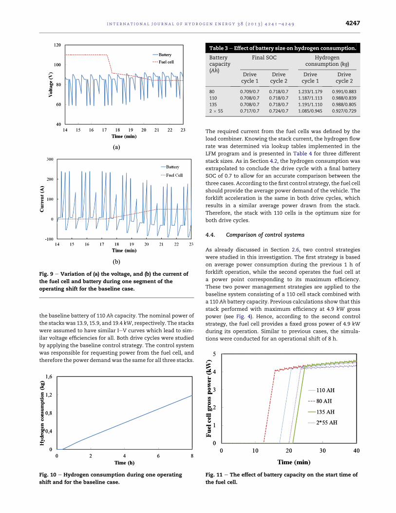
the baseline battery of 110 Ah capacity. The nominal power of

the stacks was 13.9, 15.9, and 19.4 kW, respectively. The stacks

were assumed to have similar IeV curves which lead to sim-

ilar voltage efficiencies for all. Both drive cycles were studied

by applying the baseline control strategy. The control system

was responsible for requesting power from the fuel cell, and

therefore the power demandwas the same for all three stacks.

The required current from the fuel cells was defined by the

load combiner. Knowing the stack current, the hydrogen flow

rate was determined via lookup tables implemented in the

LFM program and is presented in Table 4 for three different

stack sizes. As in Section 4.2, the hydrogen consumption was

extrapolated to conclude the drive cycle with a final battery

SOC of 0.7 to allow for an accurate comparison between the

three cases. According to the first control strategy, the fuel cell

should provide the average power demand of the vehicle. The

forklift acceleration is the same in both drive cycles, which

results in a similar average power drawn from the stack.

Therefore, the stack with 110 cells is the optimum size for

both drive cycles.

4.4. Comparison of control systems

As already discussed in Section 2.6, two control strategies

were studied in this investigation. The first strategy is based

on average power consumption during the previous 1 h of

forklift operation, while the second operates the fuel cell at

a power point corresponding to its maximum efficiency.

These two power management strategies are applied to the

baseline system consisting of a 110 cell stack combined with

a 110 Ah battery capacity. Previous calculations show that this

stack performed with maximum efficiency at 4.9 kW gross

power (see Fig. 4). Hence, according to the second control

strategy, the fuel cell provides a fixed gross power of 4.9 kW

during its operation. Similar to previous cases, the simula-

tions were conducted for an operational shift of 8 h.

Fig. 9 e Variation of (a) the voltage, and (b) the current of

the fuel cell and battery during one segment of the

operating shift for the baseline case.

Fig. 10 e Hydrogen consumption during one operating

shift and for the baseline case.

Table 3e Effect of battery size on hydrogen consumption.

Batterycapacity(Ah)

Final SOC Hydrogenconsumption (kg)

Drivecycle 1

Drivecycle 2

Drivecycle 1

Drivecycle 2

80 0.709/0.7 0.718/0.7 1.233/1.179 0.991/0.883

110 0.708/0.7 0.718/0.7 1.187/1.113 0.988/0.839

135 0.708/0.7 0.718/0.7 1.191/1.110 0.988/0.805

2 55 0.717/0.7 0.724/0.7 1.085/0.945 0.927/0.729

Fig. 11 e The effect of battery capacity on the start time of

the fuel cell.

i n t e r n a t i o n a l j o u r n a l o f h y d r o g e n en e r g y 3 8 ( 2 0 1 3 ) 4 2 4 1e4 2 4 9 4247

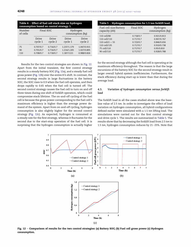
Results for the two control strategies are shown in Fig. 12.

Apart from the initial transient, the first control strategy

results in a steady battery SOC (Fig. 12a), and a steady fuel cell

gross power (Fig. 12b) over the entire 8 h shift. In contrast, the

second strategy results in large fluctuations in the battery

SOC; the SOC rises to 0.9 when the fuel cell operates, and then

drops rapidly to 0.65 when the fuel cell is turned off. The

second control strategy causes the fuel cell to turn on and off

three times during one shift of forklift operation, which could

compromise stack lifetime. The on-and-off cycling of the fuel

cell is because the gross power corresponding to the fuel cell’s

maximum efficiency is higher than the average power de-

mand of the system. Apart from on-and-off cycling, hydrogen

consumption is also slightly higher for the second control

strategy (Fig. 12c). As expected, hydrogen is consumed at

a steady rate for the first strategy, whereas it fluctuates for the

second due to the start-stop operation of the fuel cell. It is

surprising that the hydrogen consumption is actually higher

for the second strategy although the fuel cell is operating at its

maximum efficiency throughout. The reason is that the large

excursions of the battery SOC for the second strategy result in

larger overall hybrid system inefficiencies. Furthermore, the

stack efficiency during start-up is lower than that during the

average load.

4.5. Variation of hydrogen consumption versus forkliftload

The forklift load in all the cases studied above was the base-

line value of 2.5 ton. In order to investigate the effect of load

variation on hydrogen consumption, all hybrid configurations

defined earlier were simulated with a 1.5 ton lifting load. The

simulations were carried out for the first control strategy

and drive cycle 1. The results are summarized in Table 5. The

results show that by decreasing the forklift load from 2.5 ton to

1.5 ton, hydrogen consumption reduces by 21e25%. Note that

Table 4 e Effect of fuel cell stack size on hydrogenconsumption based on control strategy 1.

Numberof cells

Final SOC Hydrogenconsumption (kg)

Drivecycle 1

Drivecycle 2

Drivecycle 1

Drivecycle 2

75 0.707/0.7 0.716/0.7 1.237/1.179 1.047/0.915

90 0.701/0.7 0.716/0.7 1.214/1.205 1.027/0.895

110 0.708/0.7 0.718/0.7 1.187/1121 0.988/0.826

Fig. 12 e Comparison of results for the two control strategies: (a) Battery SOC; (b) Fuel cell gross power (c) Hydrogen

consumption.

Table 5 e Hydrogen consumption for 1.5 ton forklift load.

Fuel cell size/Batterycapacity (Ah)

Final SOC Hydrogenconsumption (kg)

110 cell/80 0.718/0.7 0.921/0.813

110 cell/110 0.717/0.7 0.907/0.767

110 cell/2 55 0.723/0.7 0.846/0.656

110 cell/135 0.717/0.7 0.910/0.738

75 cell/110 0.717/0.7 0.95/0.810

90 cell/110 0.717/0.7 0.928/0.788

i n t e rn a t i o n a l j o u r n a l o f h y d r o g e n en e r g y 3 8 ( 2 0 1 3 ) 4 2 4 1e4 2 4 94248

at the end of the operating shift, the battery SOC terminates at

different levels for the various case studied, and so the

hydrogen consumption has to be adjusted as described earlier

to allow a proper comparison. A final battery SOC of 0.7 was

assumed, and the hydrogen consumption was calculated

accordingly as shown in Table 5.

5. Conclusions

A hybrid drivetrain simulation tool called LFM was applied to

optimize a forklift system by considering system size, effi-

ciency, and hydrogen consumption. Different system topol-

ogies were studied such as the stack size, battery capacity,

drive cycle characteristics, and power management strat-

egies. The use of a larger battery delays the starting time of the

fuel cell, which reduces hydrogen consumption. However,

a larger battery increases the weight of the vehicle, hence the

tradeoff between battery capacity and weight must be con-

sidered. In our study, the case of two parallel strings of 55 Ah

batteries proved optimal due to lower internal resistance. It

was also found that the stack size of 110 cells provided the

best performance. The first control strategy results in a steady

fuel cell power and battery SOC over the entire drive cycle,

leading to reduced hydrogen consumption. In order to take

the advantage of second control strategy which forces the fuel

cell to always operate at its maximum efficiency point, the

stack size must be chosen so that the power corresponding to

itsmaximumefficiency is just slightly higher than the average

power demand of the system to prevent frequent on-and-off

cycling. For the cases studied, the second drive cycle de-

creases the hydrogen consumption by 22e26% due to its lower

operating speed and acceleration. Finally, decreasing the

forklift load from 2.5 ton to 1.5 ton reduces the hydrogen con-

sumption by 21e25%.

Acknowledgments

The authors would like to thank Højteknology Foundation for

financial support of this project, and H2 Logic A/S for their

collaboration and technical support. EH thanks Jingliang

Zhang for his help with implementing LFM for the forklift

project.

r e f e r e n c e s

[1] Wang Y, Chen K, Mishler J, Adroher X. A review of polymerelectrolyte membrane fuel cells: technology, applications,and needs on fundamental research. J Appl Energy 2011;88:981e1007.

[2] Bubna P, Brunner D, Advani SG, Prasad AK. Prediction-basedoptimal power management in a fuel cell/battery plug-inhybrid vehicle. J Power Sources 2010;195:6699e708.

[3] Ouyang M, Xu L, Li J, Lu L, Gao D, Xie Q. Performancecomparison of two fuel cell hybrid buses with differentpowertrain and energy management strategies. J PowerSources 2006;163:467e79.

[4] Schell A, Peng H, Tran D, Stamos E, Lin CC, Kim MJ. Modellingand control strategy development for fuel cell electricvehicles. Ann Rev Control 2005;29:159e68.

[5] Wu J, Zi Yuan X, JMartin J, Wang H, Zhang J, Shen J, et al.A review of PEM fuel cell durability: degradationmechanisms and mitigation strategies. J Power Sources2008;184:104e19.

[6] De Francesco M, Arato E. Start-up analysis for automotivePEM fuel cell systems. J Power Sources 2002;108:41e52.

[7] Nolan J, Kolodziej J. Modeling of an automotive fuel cellthermal system. J Power Sources 2010;195:4743e52.

[8] Wang J, Chen Y, Chen Q. A fuel cell city bus with threedrivetrain configurations. J Power Sources 2006;159:1205e13.

[9] Elgowainy A, Gaines L, Wang M. Fuel-cycle analysis of earlymarket applications of fuel cells: forklift propulsion systemsand distributed power generation. Int J Hydrogen Energy2009;34:3557e70.

[10] Keranen TM, Karimaki H, Viitakangas J, Vallet J, Ihonen J,Hyotyla P, et al. Development of integrated fuel cell hybridpower source for electric forklift. J Power Sources 2011;196:9058e68.

[11] Brown D, Alexander M, Brunner D, Advani SG, Prasad AK.Drive-train simulator for a fuel cell hybrid vehicle. J PowerSources 2008;183:275e81.

[12] Bubna P, Brunner D, Gangloff JJ, Advani SG, Prasad AK.Analysis, operation and maintenance of a fuel cell/batteryseries-hybrid bus for urban transit applications. J PowerSources 2010;195:3939e49.

i n t e r n a t i o n a l j o u r n a l o f h y d r o g e n en e r g y 3 8 ( 2 0 1 3 ) 4 2 4 1e4 2 4 9 4249

Appendix E

Paper IV

Numerical Analysis of Transport Phenomena for Design of the Ejector in a PEM FuelCell system

196

1

Numerical Analysis of Transport Phenomena for Design of the Ejector applied in a PEM

Forklift System

Elham Hosseinzadeha, Masoud Roknia, Masoud Jabbaria and Henrik Mortensenb aDepartment of Mechanical Engineering, Technical University of Denmark, Nils Koppels Allé, 2800 Kgs. Lyngby, Denmark

bH2Logic AS, 7400 Herning, Denmark Abstract In the present study, Computational Fluid Dynamics (CFD) technique is used to design an ejector for anode recirculation in an automotive PEMFC system. A CFD model is firstly established and tested against well-documented and relevant solutions from the literature, and then used for different ejector geometries under different operating conditions. Results showed that a single ejector with optimized geometry cannot cover the required recirculation in the entire range of the fuel cell current. Having two ejectors for different ranges of currents is thus proposed as an alternative solution in which the system can better take the advantage of ejectors for recirculation purpose. In addition, the operating mode of one variable nozzle ejector has been investigated and compared with aforementioned cases. The results showed that the variable nozzle ejector can work in the same operational mode as in the case with two ejectors. However, in practice it needs a more complicated control system and it is more difficult to manufacture. Keywords: Ejector, Anode recirculation, PEMFC system, CFD, Numerical analysis, Forklift Nomenclature Cw Constant D Diameter, (m) F Blending function, Eq. 13 k Kinetic energy (m2.s–2) Ma Mach number P Pressure R Gas constant (J.kmol–1K–1) Ret Turbulent Reynolds number ( – ) S Strain rate tensor (m/s) T Temperature (K) U Velocity (m/s) x Distance, (m) y Normal distance to the nearest wall, (m) Greek symbols α* Damping coefficient, Eq. 11 αd Diffuser angle, (degree) χ Entrainment ratio ( – ) ε Dissipation (m2.s–3 ) κ Specific heat gas ratio ( – )

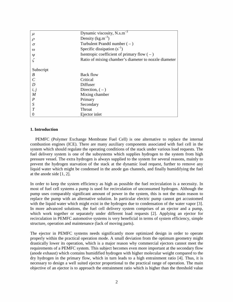
2

µ Dynamic viscosity, N.s.m–3 ρ Density (kg.m–3) σ Turbulent Prandtl number ( – ) ω Specific dissipation (s–1) ψ Isentropic coefficient of primary flow ( – ) ζ Ratio of mixing chamber’s diameter to nozzle diameter Subscript B Back flow C Critical D Diffuser i, j Direction, ( – ) M Mixing chamber P Primary S Secondary T Throat 0 Ejector inlet

1. Introduction PEMFC (Polymer Exchange Membrane Fuel Cell) is one alternative to replace the internal combustion engines (ICE). There are many auxiliary components associated with fuel cell in the system which should regulate the operating conditions of the stack under various load requests. The fuel delivery system is one of the subsystems which supplies hydrogen to the system from high pressure vessel. The extra hydrogen is always supplied to the system for several reasons, mainly to prevent the hydrogen starvation of the stack at the dynamic load request, further to remove any liquid water which might be condensed in the anode gas channels, and finally humidifying the fuel at the anode side [1, 2]. In order to keep the system efficiency as high as possible the fuel recirculation is a necessity. In most of fuel cell systems a pump is used for recirculation of unconsumed hydrogen. Although the pump uses comparably significant amount of power in the system, this is not the main reason to replace the pump with an alternative solution. In particular electric pump cannot get accustomed with the liquid water which might exist in the hydrogen due to condensation of the water vapor [3]. In more advanced solutions, the fuel cell delivery system comprises of an ejector and a pump, which work together or separately under different load requests [2]. Applying an ejector for recirculation in PEMFC automotive systems is very beneficial in terms of system efficiency, simple structure, operation and maintenance (lack of moving parts). The ejector in PEMFC systems needs significantly more optimized design in order to operate properly within the practical operation mode. A small deviation from the optimum geometry might drastically lower its operation, which is a major reason why commercial ejectors cannot meet the requirements of a PEMFC system. This subject becomes even more important at the secondary flow (anode exhaust) which contains humidified hydrogen with higher molecular weight compared to the dry hydrogen in the primary flow, which in turn leads to a high entrainment ratio [4]. Thus, it is necessary to design a well suited ejector proportional to the practical range of operation. The main objective of an ejector is to approach the entrainment ratio which is higher than the threshold value

3

at the greatest possible range of operating conditions. Modeling of an ejector can be done using different level of details. Many efforts have been made to develop ejectors for applications in refrigeration systems [5-9], but also in SOFC (Solid Oxide Fuel Cell) recirculation systems [10-12]. However, there are a few works that has been published on modeling the operational region of an ejector for the purpose of PEMFC systems [1-4]. Unlike the refrigeration and the SOFC sectors in which the convergent-divergent ejector nozzle is widely used, the convergent nozzle is mostly prevalent in PEMFC applications to avoid water condensation (due to low working temperature) in primary and secondary flow [13]. In general, ejector design is classified in to two categories, constant-area mixing ejector and constant-pressure mixing ejector which are based on the position of the nozzle exit in respect to the mixing chamber. Due to the better performance of constant-pressure mixing ejector, it is widely used in recirculation [14]. Among published papers for application of ejector in PEMFC systems, [1, 2] focused on a hybrid fuel delivery system consisting of two supplies and two recirculation lines with implementing the control system and analyzing the dynamic behavior of the system. Though, they did not provide any information about the ejector design and its development. In [4] a supersonic flow ejector for the application in a submarine PEMFC was developed. They used 1D approach for designing an ejector for relatively high power range (40 kW) without discussing its performance at low currents or startup. Low currents are basically more difficult for an ejector to operate, which is due to lower motive energy of the primary flow. On the other hand with fixed ejector geometry, it is very difficult to meet the requirements of the system in the entire range of operational conditions. Brunner et al. [3] proposed a novel variable geometry ejector for the application in a PEMFC bus, which can operate within the practical mode. They also manufactured their proposed model and validated their numerical analysis with the experimental data. Unfortunately, there is no information on start-up and low current conditions. The ejector solution in PEMFC recirculation for the forklift system, especially at the low currents, has not been investigated previously in the open literature, which is also the core motivation for the present study. In this study, the aim is to use CFD modeling for designing and developing ejector(s) for the application in PEMFC forklift system, and then analyze the entire range of operating conditions rather than the practical range only. The operating conditions of the ejector are adjusted according to the stack load variation. The calculations started with a fixed geometry for an ejector and afterwards by changing one geometrical parameter only, the influence of the corresponding parameter on the ejector performance and its operating range is analyzed. Another approach proposed and studied here was to divide the working conditions into low and high current regions and then applying two ejectors which operate together to cover the entire load variations. It was thus tried to eliminate the operating limit of a single ejector by using two ejectors working in different load ranges. Finally, another ejector with variable nozzle diameter was also studied to compare its operating performance with the proposed dual-ejectors. 2. Ejector design An ejector can be divided into four sections, Primary and secondary inlet, suction chamber, mixing section and diffuser [15]. Figure 1 shows the basic structure of an ejector.

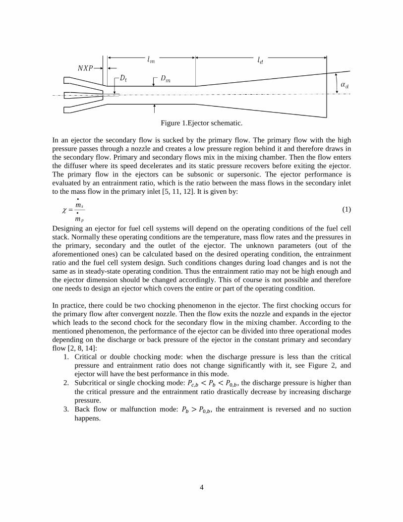
4

Figure 1.Ejector schematic.

In an ejector the secondary flow is sucked by the primary flow. The primary flow with the high pressure passes through a nozzle and creates a low pressure region behind it and therefore draws in the secondary flow. Primary and secondary flows mix in the mixing chamber. Then the flow enters the diffuser where its speed decelerates and its static pressure recovers before exiting the ejector. The primary flow in the ejectors can be subsonic or supersonic. The ejector performance is evaluated by an entrainment ratio, which is the ratio between the mass flows in the secondary inlet to the mass flow in the primary inlet [5, 11, 12]. It is given by:

p

s

m

m•

•

=χ (1)

Designing an ejector for fuel cell systems will depend on the operating conditions of the fuel cell stack. Normally these operating conditions are the temperature, mass flow rates and the pressures in the primary, secondary and the outlet of the ejector. The unknown parameters (out of the aforementioned ones) can be calculated based on the desired operating condition, the entrainment ratio and the fuel cell system design. Such conditions changes during load changes and is not the same as in steady-state operating condition. Thus the entrainment ratio may not be high enough and the ejector dimension should be changed accordingly. This of course is not possible and therefore one needs to design an ejector which covers the entire or part of the operating condition. In practice, there could be two chocking phenomenon in the ejector. The first chocking occurs for the primary flow after convergent nozzle. Then the flow exits the nozzle and expands in the ejector which leads to the second chock for the secondary flow in the mixing chamber. According to the mentioned phenomenon, the performance of the ejector can be divided into three operational modes depending on the discharge or back pressure of the ejector in the constant primary and secondary flow [2, 8, 14]:

1. Critical or double chocking mode: when the discharge pressure is less than the critical pressure and entrainment ratio does not change significantly with it, see Figure 2, and ejector will have the best performance in this mode.

2. Subcritical or single chocking mode: 𝑃𝑐,𝑏 < 𝑃𝑏 < 𝑃0,𝑏, the discharge pressure is higher than the critical pressure and the entrainment ratio drastically decrease by increasing discharge pressure.

3. Back flow or malfunction mode: 𝑃𝑏 > 𝑃0,𝑏, the entrainment is reversed and no suction happens.

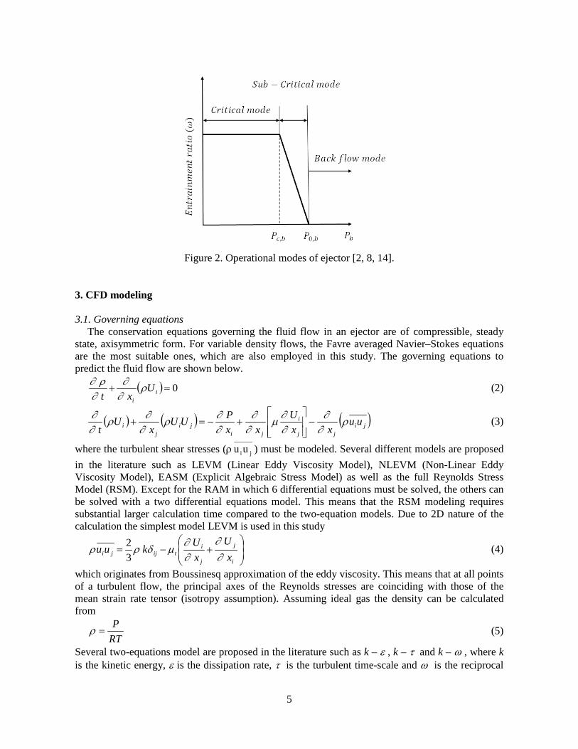
5

Figure 2. Operational modes of ejector [2, 8, 14].

3. CFD modeling 3.1. Governing equations The conservation equations governing the fluid flow in an ejector are of compressible, steady state, axisymmetric form. For variable density flows, the Favre averaged Navier–Stokes equations are the most suitable ones, which are also employed in this study. The governing equations to predict the fluid flow are shown below.

( ) 0

=+ i

i

Uxt

ρ∂∂

∂ρ∂ (2)

( ) ( ) ( )jijj

i

jiji

ji uu

xxU

xxPUU

xU

tρ

∂∂

∂∂µ

∂∂

∂∂ρ

∂∂ρ

∂∂

−

+−=+ (3)

where the turbulent shear stresses (ρ jiuu ) must be modeled. Several different models are proposed in the literature such as LEVM (Linear Eddy Viscosity Model), NLEVM (Non-Linear Eddy Viscosity Model), EASM (Explicit Algebraic Stress Model) as well as the full Reynolds Stress Model (RSM). Except for the RAM in which 6 differential equations must be solved, the others can be solved with a two differential equations model. This means that the RSM modeling requires substantial larger calculation time compared to the two-equation models. Due to 2D nature of the calculation the simplest model LEVM is used in this study

+−=

i

j

j

itijji x

UxUkuu

32

∂∂

∂∂µδρρ (4)

which originates from Boussinesq approximation of the eddy viscosity. This means that at all points of a turbulent flow, the principal axes of the Reynolds stresses are coinciding with those of the mean strain rate tensor (isotropy assumption). Assuming ideal gas the density can be calculated from

RTP

=ρ (5)

Several two-equations model are proposed in the literature such as k – ε , k – τ and k – ω , where k is the kinetic energy, ε is the dissipation rate, τ is the turbulent time-scale and ω is the reciprocal

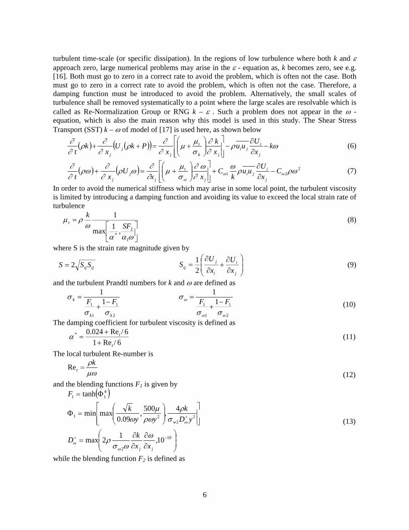
6

turbulent time-scale (or specific dissipation). In the regions of low turbulence where both k and ε approach zero, large numerical problems may arise in the ε - equation as, k becomes zero, see e.g. [16]. Both must go to zero in a correct rate to avoid the problem, which is often not the case. Both must go to zero in a correct rate to avoid the problem, which is often not the case. Therefore, a damping function must be introduced to avoid the problem. Alternatively, the small scales of turbulence shall be removed systematically to a point where the large scales are resolvable which is called as Re-Normalization Group or RNG k – ε . Such a problem does not appear in the ω - equation, which is also the main reason why this model is used in this study. The Shear Stress Transport (SST) k – ω of model of [17] is used here, as shown below

( ) ( )( ) ωρ∂∂

σµµ

∂∂ρ

∂∂ρ

∂∂ k

xUuu

xk

xPkU

xk

t j

iji

jk

t

jj

j

−∂∂

−

+=++

(6)

( ) ( ) 221

ρωρω∂ω∂

σµµ

∂∂ωρ

∂∂ρω

∂∂

ωωω

CxUuu

kC

xxU

xt j

iji

j

t

jj

j

−∂∂

+

+=+ (7)

In order to avoid the numerical stiffness which may arise in some local point, the turbulent viscosity is limited by introducing a damping function and avoiding its value to exceed the local strain rate of turbulence

=

ωααω

ρµτ

1

2* ,1max

1 SF

k (8)

where S is the strain rate magnitude given by

ijij SSS 2=

∂∂

+∂

∂=

j

i

i

jij x

UxU

S21 (9)

and the turbulent Prandtl numbers for k and ω are defined as

2

1

1

1 11

kk

k FFσσ

σ−

+=

2

1

1

1 11

ωω

ω

σσ

σ FF −+

= (10)

The damping coefficient for turbulent viscosity is defined as

6/Re1

6/Re024.0*

t

t

++

=α (11)

The local turbulent Re-number is

µωρk

t =Re (12)

and the blending functions F1 is given by

( )

∂∂

∂∂

=

=Φ

Φ=

−+

+

10

2

22

21

411

10,12max

4,500,09.0

maxmin

tanh

jj

w

xxkD

yDk

yyk

F

ωωσ

ρ

σρ

ρωµ

ω

ωω

ω (13)

while the blending function F2 is defined as

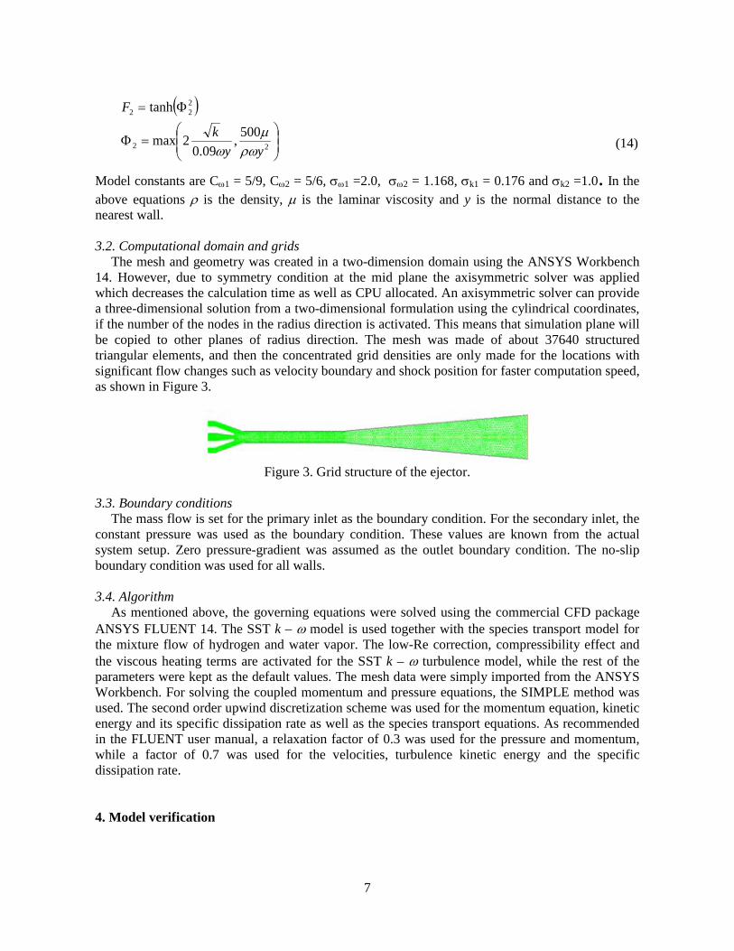
7

( )

=Φ

Φ=

22

222

500,09.0

2max

tanh

yyk

F

ρωµ

ω (14)

Model constants are Cω1 = 5/9, Cω2 = 5/6, σω1 =2.0, σω2 = 1.168, σk1 = 0.176 and σk2 =1.0. In the above equations ρ is the density, µ is the laminar viscosity and y is the normal distance to the nearest wall. 3.2. Computational domain and grids The mesh and geometry was created in a two-dimension domain using the ANSYS Workbench 14. However, due to symmetry condition at the mid plane the axisymmetric solver was applied which decreases the calculation time as well as CPU allocated. An axisymmetric solver can provide a three-dimensional solution from a two-dimensional formulation using the cylindrical coordinates, if the number of the nodes in the radius direction is activated. This means that simulation plane will be copied to other planes of radius direction. The mesh was made of about 37640 structured triangular elements, and then the concentrated grid densities are only made for the locations with significant flow changes such as velocity boundary and shock position for faster computation speed, as shown in Figure 3.

Figure 3. Grid structure of the ejector.

3.3. Boundary conditions The mass flow is set for the primary inlet as the boundary condition. For the secondary inlet, the constant pressure was used as the boundary condition. These values are known from the actual system setup. Zero pressure-gradient was assumed as the outlet boundary condition. The no-slip boundary condition was used for all walls. 3.4. Algorithm As mentioned above, the governing equations were solved using the commercial CFD package ANSYS FLUENT 14. The SST k – ω model is used together with the species transport model for the mixture flow of hydrogen and water vapor. The low-Re correction, compressibility effect and the viscous heating terms are activated for the SST k – ω turbulence model, while the rest of the parameters were kept as the default values. The mesh data were simply imported from the ANSYS Workbench. For solving the coupled momentum and pressure equations, the SIMPLE method was used. The second order upwind discretization scheme was used for the momentum equation, kinetic energy and its specific dissipation rate as well as the species transport equations. As recommended in the FLUENT user manual, a relaxation factor of 0.3 was used for the pressure and momentum, while a factor of 0.7 was used for the velocities, turbulence kinetic energy and the specific dissipation rate. 4. Model verification

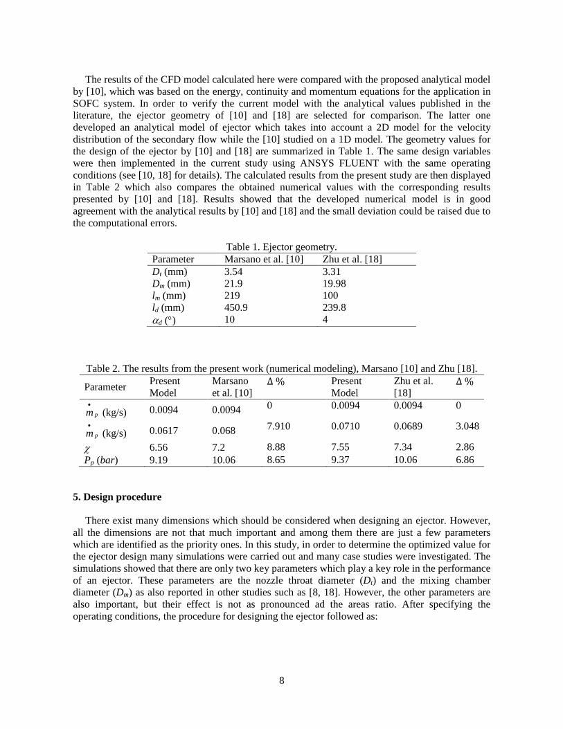
8

The results of the CFD model calculated here were compared with the proposed analytical model by [10], which was based on the energy, continuity and momentum equations for the application in SOFC system. In order to verify the current model with the analytical values published in the literature, the ejector geometry of [10] and [18] are selected for comparison. The latter one developed an analytical model of ejector which takes into account a 2D model for the velocity distribution of the secondary flow while the [10] studied on a 1D model. The geometry values for the design of the ejector by [10] and [18] are summarized in Table 1. The same design variables were then implemented in the current study using ANSYS FLUENT with the same operating conditions (see [10, 18] for details). The calculated results from the present study are then displayed in Table 2 which also compares the obtained numerical values with the corresponding results presented by [10] and [18]. Results showed that the developed numerical model is in good agreement with the analytical results by [10] and [18] and the small deviation could be raised due to the computational errors.

Table 1. Ejector geometry. Parameter Marsano et al. [10] Zhu et al. [18] Dt (mm) 3.54 3.31 Dm (mm) 21.9 19.98 lm (mm) 219 100 ld (mm) 450.9 239.8 αd (°) 10 4

Table 2. The results from the present work (numerical modeling), Marsano [10] and Zhu [18].

Parameter Present Model

Marsano et al. [10]

∆ %

Present Model

Zhu et al. [18]

∆ %

pm•

(kg/s) 0.0094 0.0094 0 0.0094 0.0094 0

pm•

(kg/s) 0.0617 0.068 7.910 0.0710 0.0689 3.048

χ 6.56 7.2 8.88 7.55 7.34 2.86 Pp (bar) 9.19 10.06 8.65 9.37 10.06 6.86

5. Design procedure There exist many dimensions which should be considered when designing an ejector. However, all the dimensions are not that much important and among them there are just a few parameters which are identified as the priority ones. In this study, in order to determine the optimized value for the ejector design many simulations were carried out and many case studies were investigated. The simulations showed that there are only two key parameters which play a key role in the performance of an ejector. These parameters are the nozzle throat diameter (Dt) and the mixing chamber diameter (Dm) as also reported in other studies such as [8, 18]. However, the other parameters are also important, but their effect is not as pronounced ad the areas ratio. After specifying the operating conditions, the procedure for designing the ejector followed as:

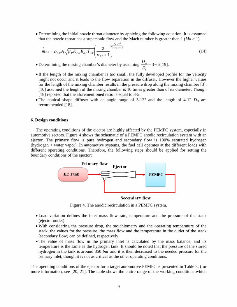
9

• Determining the initial nozzle throat diameter by applying the following equation. It is assumed that the nozzle throat has a supersonic flow and the Mach number is greater than 1 (Ma > 1).

( )121

0,0,,0,0,1,

0,

0,

12 −

+

•

+=

P

P

PPPgPPtPP TRKAm

κκ

κψρ (14)

• Determining the mixing chamber’s diameter by assuming 63−=t

m

DD

[19].

• If the length of the mixing chamber is too small, the fully developed profile for the velocity might not occur and it leads to the flow separation in the diffuser. However the higher values for the length of the mixing chamber results in the pressure drop along the mixing chamber [3]. [10] assumed the length of the mixing chamber is 10 times greater than of its diameter. Though [18] reported that the aforementioned ratio is equal to 3-5.

• The conical shape diffuser with an angle range of 5-12° and the length of 4-12 Dm are recommended [18].

6. Design conditions The operating conditions of the ejector are highly affected by the PEMFC system, especially in automotive sectors. Figure 4 shows the schematic of a PEMFC anodic recirculation system with an ejector. The primary flow is pure hydrogen and secondary flow is 100% saturated hydrogen (hydrogen + water vapor). In automotive systems, the fuel cell operates at the different loads with different operating conditions. Therefore, the following steps should be applied for setting the boundary conditions of the ejector:

Figure 4. The anodic recirculation in a PEMFC system.

• Load variation defines the inlet mass flow rate, temperature and the pressure of the stack

(ejector outlet). • With considering the pressure drop, the stoichiometry and the operating temperature of the

stack, the values for the pressure, the mass flow and the temperature in the outlet of the stack (secondary flow) can be defined, respectively.

• The value of mass flow in the primary inlet is calculated by the mass balance, and its temperature is the same as the hydrogen tank. It should be noted that the pressure of the stored hydrogen in the tank is around 350 bar and it is then decreased to the needed pressure for the primary inlet, though it is not as critical as the other operating conditions.

The operating conditions of the ejector for a target automotive PEMFC is presented in Table 3, (for more information, see [20, 21]. The table shows the entire range of the working conditions which

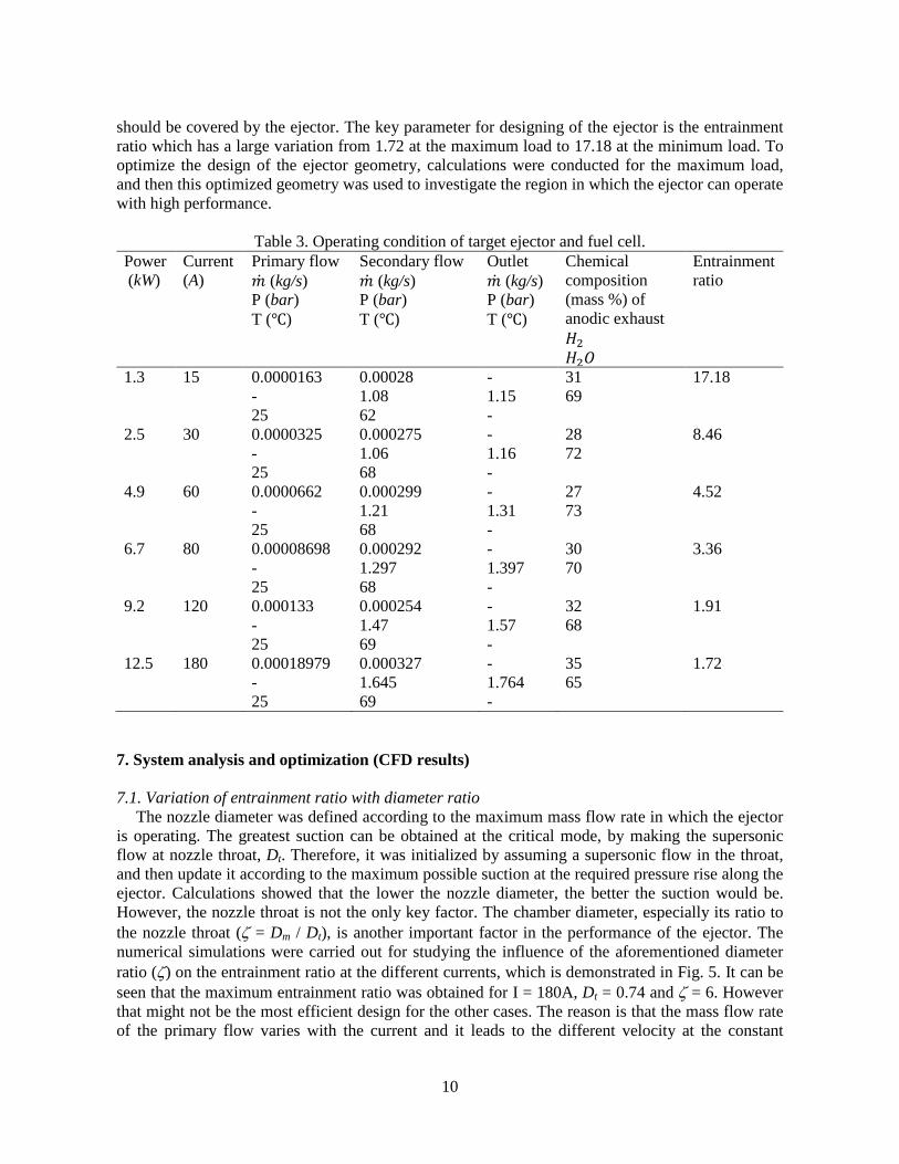
10

should be covered by the ejector. The key parameter for designing of the ejector is the entrainment ratio which has a large variation from 1.72 at the maximum load to 17.18 at the minimum load. To optimize the design of the ejector geometry, calculations were conducted for the maximum load, and then this optimized geometry was used to investigate the region in which the ejector can operate with high performance.

Table 3. Operating condition of target ejector and fuel cell. Power (kW)

Current (A)

Primary flow (kg/s) P (bar) T ()

Secondary flow (kg/s) P (bar) T ()

Outlet (kg/s) P (bar) T ()

Chemical composition (mass %) of anodic exhaust 𝐻2 𝐻2𝑂

Entrainment ratio

1.3 15 0.0000163 - 25

0.00028 1.08 62

- 1.15 -

31 69

17.18

2.5 30 0.0000325 - 25

0.000275 1.06 68

- 1.16 -

28 72

8.46

4.9 60 0.0000662 - 25

0.000299 1.21 68

- 1.31 -

27 73

4.52

6.7 80 0.00008698 - 25

0.000292 1.297 68

- 1.397 -

30 70

3.36

9.2 120 0.000133 - 25

0.000254 1.47 69

- 1.57 -

32 68

1.91

12.5 180 0.00018979 - 25

0.000327 1.645 69

- 1.764 -

35 65

1.72

7. System analysis and optimization (CFD results) 7.1. Variation of entrainment ratio with diameter ratio The nozzle diameter was defined according to the maximum mass flow rate in which the ejector is operating. The greatest suction can be obtained at the critical mode, by making the supersonic flow at nozzle throat, Dt. Therefore, it was initialized by assuming a supersonic flow in the throat, and then update it according to the maximum possible suction at the required pressure rise along the ejector. Calculations showed that the lower the nozzle diameter, the better the suction would be. However, the nozzle throat is not the only key factor. The chamber diameter, especially its ratio to the nozzle throat (ζ = Dm / Dt), is another important factor in the performance of the ejector. The numerical simulations were carried out for studying the influence of the aforementioned diameter ratio (ζ) on the entrainment ratio at the different currents, which is demonstrated in Fig. 5. It can be seen that the maximum entrainment ratio was obtained for I = 180A, Dt = 0.74 and ζ = 6. However that might not be the most efficient design for the other cases. The reason is that the mass flow rate of the primary flow varies with the current and it leads to the different velocity at the constant

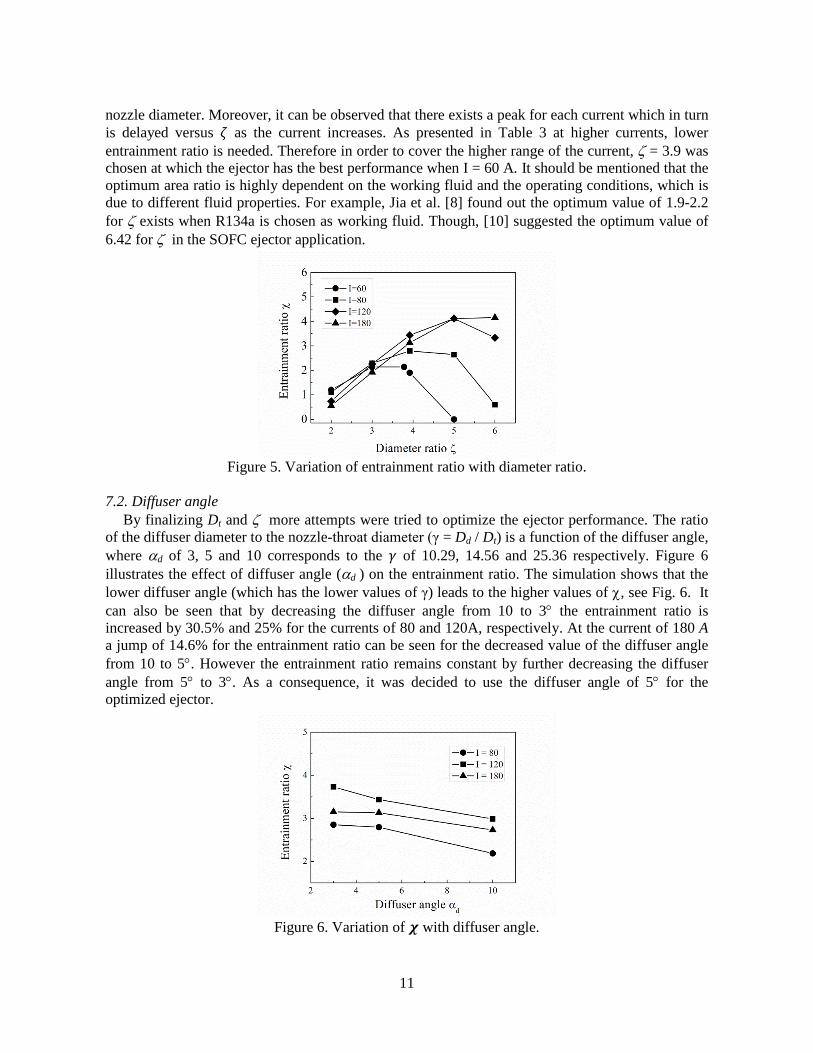
11

nozzle diameter. Moreover, it can be observed that there exists a peak for each current which in turn is delayed versus 𝜁 as the current increases. As presented in Table 3 at higher currents, lower entrainment ratio is needed. Therefore in order to cover the higher range of the current, ζ = 3.9 was chosen at which the ejector has the best performance when I = 60 A. It should be mentioned that the optimum area ratio is highly dependent on the working fluid and the operating conditions, which is due to different fluid properties. For example, Jia et al. [8] found out the optimum value of 1.9-2.2 for ζ exists when R134a is chosen as working fluid. Though, [10] suggested the optimum value of 6.42 for ζ in the SOFC ejector application.

Figure 5. Variation of entrainment ratio with diameter ratio.

7.2. Diffuser angle By finalizing Dt and ζ more attempts were tried to optimize the ejector performance. The ratio of the diffuser diameter to the nozzle-throat diameter (γ = Dd / Dt) is a function of the diffuser angle, where αd of 3, 5 and 10 corresponds to the 𝛾 of 10.29, 14.56 and 25.36 respectively. Figure 6 illustrates the effect of diffuser angle (αd ) on the entrainment ratio. The simulation shows that the lower diffuser angle (which has the lower values of γ) leads to the higher values of χ, see Fig. 6. It can also be seen that by decreasing the diffuser angle from 10 to 3° the entrainment ratio is increased by 30.5% and 25% for the currents of 80 and 120A, respectively. At the current of 180 A a jump of 14.6% for the entrainment ratio can be seen for the decreased value of the diffuser angle from 10 to 5°. However the entrainment ratio remains constant by further decreasing the diffuser angle from 5° to 3°. As a consequence, it was decided to use the diffuser angle of 5° for the optimized ejector.

Figure 6. Variation of 𝝌 with diffuser angle.

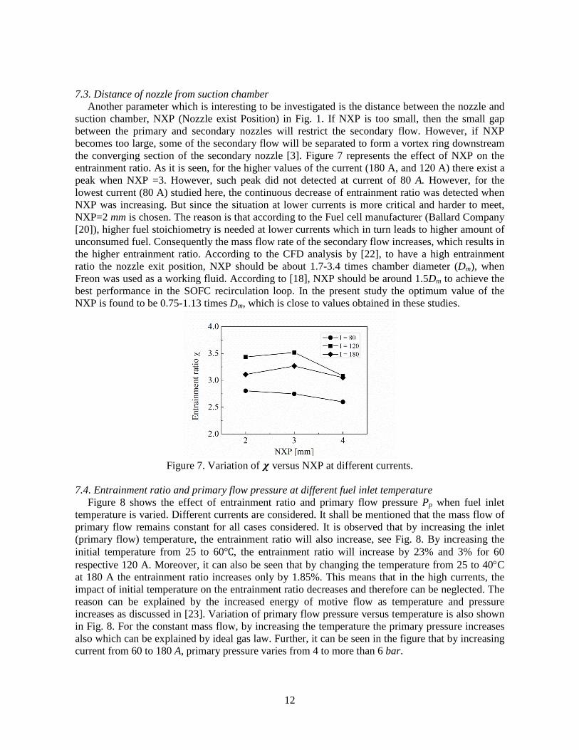
12

7.3. Distance of nozzle from suction chamber Another parameter which is interesting to be investigated is the distance between the nozzle and suction chamber, NXP (Nozzle exist Position) in Fig. 1. If NXP is too small, then the small gap between the primary and secondary nozzles will restrict the secondary flow. However, if NXP becomes too large, some of the secondary flow will be separated to form a vortex ring downstream the converging section of the secondary nozzle [3]. Figure 7 represents the effect of NXP on the entrainment ratio. As it is seen, for the higher values of the current (180 A, and 120 A) there exist a peak when NXP =3. However, such peak did not detected at current of 80 A. However, for the lowest current (80 A) studied here, the continuous decrease of entrainment ratio was detected when NXP was increasing. But since the situation at lower currents is more critical and harder to meet, NXP=2 mm is chosen. The reason is that according to the Fuel cell manufacturer (Ballard Company [20]), higher fuel stoichiometry is needed at lower currents which in turn leads to higher amount of unconsumed fuel. Consequently the mass flow rate of the secondary flow increases, which results in the higher entrainment ratio. According to the CFD analysis by [22], to have a high entrainment ratio the nozzle exit position, NXP should be about 1.7-3.4 times chamber diameter (Dm), when Freon was used as a working fluid. According to [18], NXP should be around 1.5Dm to achieve the best performance in the SOFC recirculation loop. In the present study the optimum value of the NXP is found to be 0.75-1.13 times Dm, which is close to values obtained in these studies.

Figure 7. Variation of 𝝌 versus NXP at different currents.

7.4. Entrainment ratio and primary flow pressure at different fuel inlet temperature Figure 8 shows the effect of entrainment ratio and primary flow pressure Pp when fuel inlet temperature is varied. Different currents are considered. It shall be mentioned that the mass flow of primary flow remains constant for all cases considered. It is observed that by increasing the inlet (primary flow) temperature, the entrainment ratio will also increase, see Fig. 8. By increasing the initial temperature from 25 to 60, the entrainment ratio will increase by 23% and 3% for 60 respective 120 A. Moreover, it can also be seen that by changing the temperature from 25 to 40°C at 180 A the entrainment ratio increases only by 1.85%. This means that in the high currents, the impact of initial temperature on the entrainment ratio decreases and therefore can be neglected. The reason can be explained by the increased energy of motive flow as temperature and pressure increases as discussed in [23]. Variation of primary flow pressure versus temperature is also shown in Fig. 8. For the constant mass flow, by increasing the temperature the primary pressure increases also which can be explained by ideal gas law. Further, it can be seen in the figure that by increasing current from 60 to 180 A, primary pressure varies from 4 to more than 6 bar.

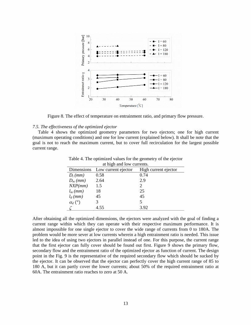
13

Figure 8. The effect of temperature on entrainment ratio, and primary flow pressure. 7.5. The effectiveness of the optimized ejector Table 4 shows the optimized geometry parameters for two ejectors; one for high current (maximum operating conditions) and one for low current (explained below). It shall be note that the goal is not to reach the maximum current, but to cover full recirculation for the largest possible current range.

Table 4. The optimized values for the geometry of the ejector at high and low currents.

Dimensions Low current ejector High current ejector Dt (mm) 0.58 0.74 Dm (mm) 2.64 2.9 NXP(mm) 1.5 2 lm (mm) 18 25 ld (mm) 45 45 αd (°) 3 5 ζ 4.55 3.92

After obtaining all the optimized dimensions, the ejectors were analyzed with the goal of finding a current range within which they can operate with their respective maximum performance. It is almost impossible for one single ejector to cover the wide range of currents from 0 to 180A. The problem would be more sever at low currents wherein a high entrainment ratio is needed. This issue led to the idea of using two ejectors in parallel instead of one. For this purpose, the current range that the first ejector can fully cover should be found out first. Figure 9 shows the primary flow, secondary flow and the entrainment ratio of the optimized ejector as function of current. The design point in the Fig. 9 is the representative of the required secondary flow which should be sucked by the ejector. It can be observed that the ejector can perfectly cover the high current range of 85 to 180 A, but it can partly cover the lower currents; about 50% of the required entrainment ratio at 60A. The entrainment ratio reaches to zero at 50 A.

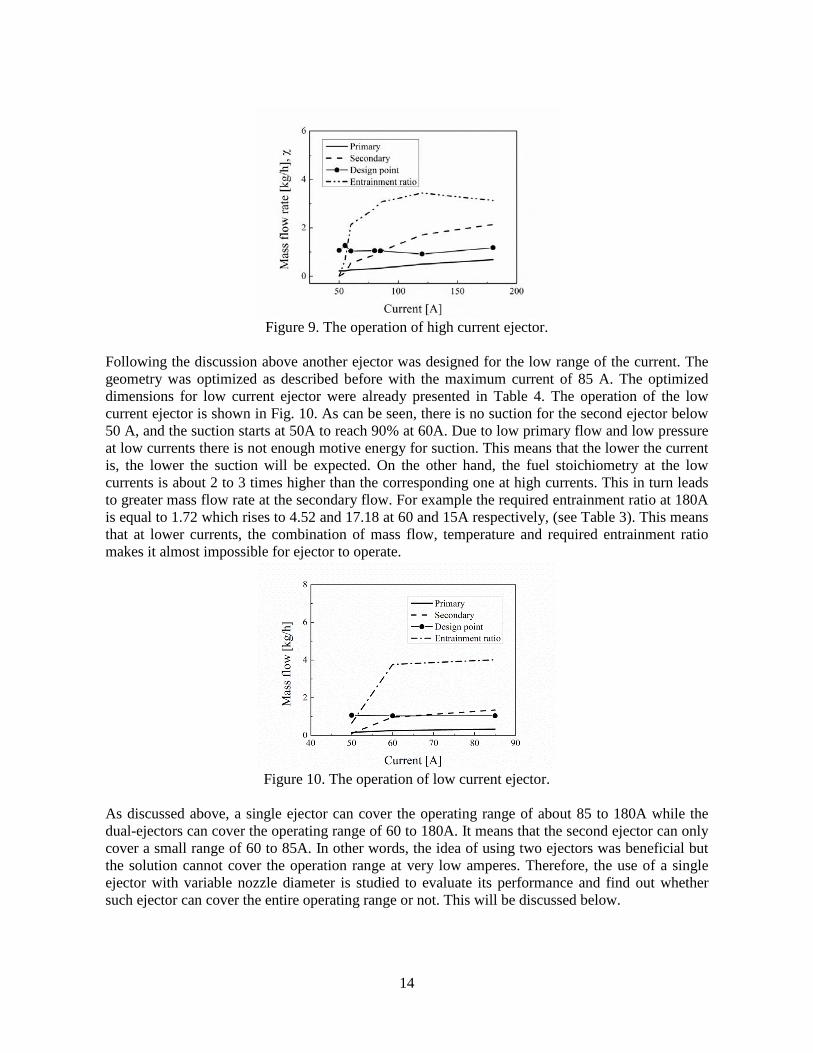
14

Figure 9. The operation of high current ejector.

Following the discussion above another ejector was designed for the low range of the current. The geometry was optimized as described before with the maximum current of 85 A. The optimized dimensions for low current ejector were already presented in Table 4. The operation of the low current ejector is shown in Fig. 10. As can be seen, there is no suction for the second ejector below 50 A, and the suction starts at 50A to reach 90% at 60A. Due to low primary flow and low pressure at low currents there is not enough motive energy for suction. This means that the lower the current is, the lower the suction will be expected. On the other hand, the fuel stoichiometry at the low currents is about 2 to 3 times higher than the corresponding one at high currents. This in turn leads to greater mass flow rate at the secondary flow. For example the required entrainment ratio at 180A is equal to 1.72 which rises to 4.52 and 17.18 at 60 and 15A respectively, (see Table 3). This means that at lower currents, the combination of mass flow, temperature and required entrainment ratio makes it almost impossible for ejector to operate.

Figure 10. The operation of low current ejector.

As discussed above, a single ejector can cover the operating range of about 85 to 180A while the dual-ejectors can cover the operating range of 60 to 180A. It means that the second ejector can only cover a small range of 60 to 85A. In other words, the idea of using two ejectors was beneficial but the solution cannot cover the operation range at very low amperes. Therefore, the use of a single ejector with variable nozzle diameter is studied to evaluate its performance and find out whether such ejector can cover the entire operating range or not. This will be discussed below.

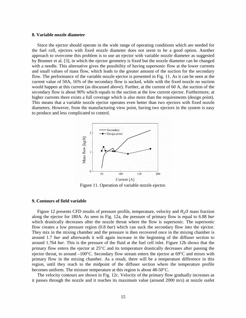
15

8. Variable nozzle diameter Since the ejector should operate in the wide range of operating conditions which are needed for the fuel cell, ejectors with fixed nozzle diameter does not seem to be a good option. Another approach to overcome this problem is to use an ejector with variable nozzle diameter as suggested by Brunner et al. [3], in which the ejector geometry is fixed but the nozzle diameter can be changed with a needle. This alternative gives the possibility of having supersonic flow at the lower currents and small values of mass flow, which leads to the greater amount of the suction for the secondary flow. The performance of the variable nozzle ejector is presented in Fig. 11. As it can be seen at the current value of 50A, 16% of the secondary flow is sucked, while with the fixed nozzle no suction would happen at this current (as discussed above). Further, at the current of 60 A, the suction of the secondary flow is about 90% which equals to the suction at the low current ejector. Furthermore, at higher currents there exists a full coverage which is also more than the requirements (design point). This means that a variable nozzle ejector operates even better than two ejectors with fixed nozzle diameters. However, from the manufacturing view point, having two ejectors in the system is easy to produce and less complicated to control.

Figure 11. Operation of variable nozzle ejector.

9. Contours of field variable Figure 12 presents CFD results of pressure profile, temperature, velocity and 𝐻2𝑂 mass fraction along the ejector for 180A. As seen in Fig. 12a, the pressure of primary flow is equal to 6.88 bar which drastically decreases after the nozzle throat where the flow is supersonic. The supersonic flow creates a low pressure region (0.8 bar) which can suck the secondary flow into the ejector. They mix in the mixing chamber and the pressure is then recovered once in the mixing chamber is around 1.7 bar and afterwards it will again increase in the beginning of the diffuser section to around 1.764 bar. This is the pressure of the fluid at the fuel cell inlet. Figure 12b shows that the primary flow enters the ejector at 25°C and its temperature drastically decreases after passing the ejector throat, to around –100°C. Secondary flow stream enters the ejector at 69°C and mixes with primary flow in the mixing chamber. As a result, there will be a temperature difference in this region, until they reach to the midpoint of the diffuser section where the temperature profile becomes uniform. The mixture temperature at this region is about 48-50°C. The velocity contours are shown in Fig. 12c. Velocity of the primary flow gradually increases as it passes through the nozzle and it reaches its maximum value (around 2000 m/s) at nozzle outlet

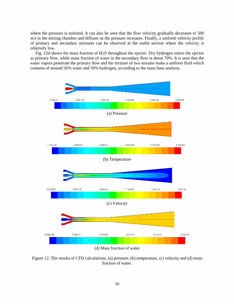
16

where the pressure is minimal. It can also be seen that the flow velocity gradually decreases to 500 m/s in the mixing chamber and diffuser as the pressure increases. Finally, a uniform velocity profile of primary and secondary mixtures can be observed at the outlet section where the velocity is relatively low. Fig. 12d shows the mass fraction of H2O throughout the ejector. Dry hydrogen enters the ejector as primary flow, while mass fraction of water in the secondary flow is about 70%. It is seen that the water vapors penetrate the primary flow and the mixture of two streams make a uniform fluid which contains of around 50% water and 50% hydrogen, according to the mass base analysis.

(a) Pressure

(b) Temperature

(c) Velocity

(d) Mass fraction of water

Figure 12. The results of CFD calculations, (a) pressure, (b) temperature, (c) velocity and (d) mass

fraction of water.

17

10. Conclusion In this study, CFD technique has been used to design and analyze an ejector for anode recirculation of PEMFC system applied in a forklift truck. Since the ejector is integrated in the PEMFC system, its operating conditions should be adjusted according to the fuel cell load fluctuations to cover the current variation of the stack from 0-180 A. In order for the ejector to operate in the largest possible range of load, different approaches (with fixed nozzle and variable nozzle ejectors) have been investigated. For the first approach an ejector has been designed so that it could operate at the maximum load and mass flow rate. Then different geometries have been investigated in order to optimize the ejector. The optimization is carried out not only by considering the best performance of ejector at maximum load with operation in the larger range as priority, but also catching the design point at maximum load even though it does not have the best efficiency at such point. The geometry analysis showed that diameter ratios (ζ) is the key parameter in designing the ejector, and by choosing ζ = 3.9 at Dt = 0.74 the ejector can operate from 85-180A properly. In order to increase the operating range, another ejector was designed for maximum current of 85A. By optimization the second ejector it was found that it could operate 100% at 85A and down to 90% at 60A. The third approach was applying an ejector with variable nozzle diameter. The results showed that such ejector can also operate 100% at 180A down to 90% at 60A. However, in practice it is more difficult to manufacture an ejector with variable nozzle compared to an ejector with the fixed nozzle diameter, but it could be the best choice for having the greatest entrainment ratio in the system. Acknowledgement

The authors would like to acknowledge the Danish Advanced Technology Foundation (Højteknologifonden) for financial support of this project, H2Logic Company for their collaboration and technical support. Also special thanks to Douglas A. Brunner for his support and guidance during this project. 11. References [1] J. He, S.Y. Choe, C.O. Hong, Analysis and control of a hybrid fuel delivery system for a

polymer electrolyte membrane fuel cell, Journal of Power Sources 185 (2008) 973–984. [2] J. He, J. Ahn, S.Y. Choe, Analysis and control of a fuel delivery system considering a two-

phase anode model of the polymer electrolyte membrane fuel cell stack, Journal of Power Sources 196 (2011) 4655–4670.

[3] D.A. Brunner, S. Marcks, M. Bajpai, A.K. Prasad, S.G. Advani, Design and characterization of an electronically controlled variable flow rate ejector for fuel cell applications, International Journal of Hydrogen Energy 37 (2012) 4457-4466.

[4] M. Kim, Y.J. Sohn, C.W. Cho, W.Y. Lee, C.S. Kim, Customized design for the ejector to recirculate a humidified hydrogen fuel in a submarine PEMFC, Journal fo Power Sources 176 (2008) 529–533.

[5] D.W. Sun, Comparative study of the performance of an ejector refrigeration cycle operating with various refrigerants, Journal of Energy Conversion & Management 40 (1999) 873-884.

[6] D.W. Sun, Experimental investigation of the performance characteristics of a steam jet refrigeration system, Journal of Energy Sources 19 (2007) 349-367.

18

[7] M. Colarossi, N. Trask, D.P. Schmidt, M.J. Bergander, Multidimensional modeling of condensing two-phase ejector flow, International Journal of Refrigeration 35 (2012) 290-299.

[8] Y. Jia, C. Wenjian, Area ratio effects to the performance of air-cooled ejector refrigeration cycle with R134a refrigerant, Journal of Energy Conversion and Management 53 (2012) 240–246.

[9] G. Grazzini, A. Milazzo, D. Paganini, Design of an ejector cycle refrigeration system, Journal of Energy Conversion and Management 54 (2012) 38–46.

[10] F. Marsano, L. Magistri, A.F. Massardo, Ejector performance influence on a solid oxide fuel cell anodic recirculation system, Journal of Power Sources 129 (2004) 216–228.

[11] J. Milewski, A. Miller, J. Sałaci´nski, Off-design analysis of SOFC hybrid system, International Journal of Hydrogen Energy 32 (2007) 687–698.

[12] Y. Zhu, Y. Li, W. Cai, Control oriented modeling of ejector in anode gas recirculation solid oxygen fuel cell systems, Journal of Energy Conversion and Management 52 (2011) 1881–1889.

[13] Y. Zhu, Y. Li, New theoretical model for convergent nozzle ejector in the proton exchange membrane fuel cell system, Journal of Power Sources 191 (2009) 510–519.

[14] B.J. Huang, J.M. Chang, C.P. Wang, V.A. Petrenko, A 1-D analysis of ejector performance, International Journal of Refrigeration 22 (1999) 354–364.

[15] J. Garcı´a del Valle, J.M. Sa´ iz Jabardo, F. Castro Ruiz, J.S. Jose´ Alonso, A one dimensional model for the determination of an ejector entrainment ratio, International Journal of Refrigeration 35 (2012) 772-784.

[16] M. Rokni, B. Sunden, On Developments of k-tau and k-omega models for near-wall turbulence of duct flows, International Journal of Phenomena 11 (2009) 233-253.

[17] F.R. Mentor, Two-equation eddy-viscosity turbulence models for engineering applications, AIAA Journal 32 (8) (1994) 1598-1605.

[18] Y. Zhu, W. Cai, C. Wen, Y. Li, Fuel ejector design and simulation model for anodic recirculation SOFC system, Journal of Power Sources 173 (2007) 437–449.

[19] G.E. Alves, Ejector design and performance, in: Fluid and practicle mechanism , Newark, DE, University of Delaware , 1951, pp. 69-79.

[20] Mark9 SSL™ of Ballard Company, Product manual and integration guide, 2008. [21] E. Hosseinzadeh, M. Rokni, Development and validation of a simple analytical model of the

Proton Exchange Membrane Fuel Cell (PEMFC) in a fork-lift truck power system, International Journal of Green Energy 2012, In press.

[22] Y. Zhu, W. Cai, C. Wen, Y. Li, Numerical investigation of geometry parameters for design of high performance ejectors, Journal of Applied Thermal Engineering 29 (2009) 898–905.

[23] M. Nakagawa, A.R. Marasigan, T. Matsukawa, A. Kurashina, Experimental investigation on the effect of mixing length on the performance of two-phase ejector for CO2 refrigeration cycle with and without heat exchanger, International Journal of Refrigeration 34 (2011) 1604-1613.

Appendix F

Paper V

Proton Exchange Membrane Fuel Cells Applied for Transport Sector

215

5th International Ege Energy Symposium and Exhibition (IEESE-5) 27-30 June 2010

Pamukkale University, Denizli, Turkey

Proton Exchange Membrane Fuel Cells Applied for Transport Sector

Elham Hoseinzadeh, Masoud Rokni

Technical University of Denmark, Dept. of Mechanical Engineering, Thermal Energy System, Building 403, 2800 Kgs, Lyngby, Denmark

ehos@mek.dtu.dk, mr@mek.dtu.dk

ABSTRACT – A thermodynamic analysis of a PEMFC (proton exchange membrane fuel cell) is investigated. PEMFC may be the most promising technology for fuel cell automotive systems, which is operating at quite low temperatures, (between 60 to 80). In this study the fuel cell motive power part of a lift truck has been investigated. The fuel cell stack used in this model is developed using a Ballard PEMFC [1], so that the equations used in the stack modeling are derived from the experimental data. The stack can produce 3 to 15 kilowatt electricity depending on the number of cells used in the stack. Some of the electricity will be consumed by pumps and compressors in the system. Generally the whole system can be separated in three parts, cathode circuit, anode circuit and cooling loops. In this paper the effect of operating condi-tions and anode recirculation on power production as well as system efficiency have been investigated. In addition, differ-ent stack design schemes have been proposed and their effect on system efficiency has been investigated.

Key words: PEMFC, fuel cell, cooling loop, anode recirculation, system design, serial stacks

I. INTRODUCTION

Today global warming is one of the greatest concerns of the world and fossil fuel emissions are the most im-portant human cause of it. Finding an alternative source to fossil fuels is inevitable in our automobile industry, which leads to the next generation vehicles. Fuel cells, and espe-cially PEM (proton exchange membrane) fuel cells, are considered as possible environmentally friendly generators for the propulsion of vehicles in the future and they are getting more attention because of low operating tempera-ture and pressure which provide the possibility of using the cheaper components. But still Lack of hydrogen infra-structure is considered the biggest obstacle for introduc-tion of fuel cell vehicles and due to its low temperature operation there is no internal reforming inside of it and just pure hydrogen can be used as a fuel which is of course expensive.

Fuel cells offer several advantages over either internal combustion engine generators (noise, expected higher reliability and lower maintenance) or batteries (weight, lifetime, maintenance). But today PEM fuel cell automo-tive systems are too expensive for wide-spread marketing. These systems still need some improvement so that they can compete with internal combustion engines.

There are two distinct approaches for modeling the fuel cell systems. The first one is modeling the details of individual stack and considering the operating conditions to determine the current-voltage curve and the second one is modeling the fuel cell system based on voltage-current output for existing fuel cells and making models for auxil-

iary components. But no great attention has been turned to the balance of plant system which makes the fuel cell system work efficiently.

In [2] results of recent studies of PEM fuel cell-powered vehicle performance using direct-hydrogen fuel-ing and on-board methanol reforming have been summa-rized. In that research, control of auxiliary components is found to provide the greatest opportunity for improved performance.

A fuel cell stack is obviously the heart of a fuel cell system; however, without the supporting equipment the stack itself would not be very useful. The fuel cell system typically involves the following subsystems: – Oxidant supply (oxygen or air) – Fuel supply (hydrogen or hydrogen-rich gas) – Heat management – Water management – Power conditioning – Instrumentation and controls

Following the first target some researches have been presented in [3]-[5], describing the details of fuel cell stack operation. In [3] a three-dimensional CFD model of PEM fuel cell is developed by taking into account the electro-chemical, mass and heat transfer phenomena occurring in all of its regions simultaneously and also the effect of operating conditions, temperatures and pressures on the stack efficiency. In [4] water and thermal management model for a Ballard PEM fuel cell stack was developed to investigate its performance. In [5] the mass transport phe-nomenon through the membrane has been studied. Accord-

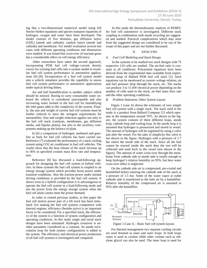
5th International Ege Energy Symposium and Exhibition (IEESE-5) 27-30 June 2010

Pamukkale University, Denizli, Turkey

ing that a two-dimensional numerical model using full Navier-Stokes equations and species transport equations of hydrogen, oxygen and water have been developed. The model consists of five domains, gas diffusion layers (GDL) (anode and cathode), catalyst layers (anode and cathode) and membrane. For model evaluation several test cases with different operating conditions and dimensions were studied. It was found that cross-over of reactant gases has a considerable effect on cell energy efficiency.

Other researchers have taken the second approach, incorporating PEM fuel cell voltage–current density curves for existing fuel cells into a system model to exam-ine fuel cell system performance in automotive applica-tions [6]–[8]. Incorporation of a fuel cell system model into a vehicle simulator provides the capability to assess fuel cell system performance in automotive applications under typical driving duties.

Air and fuel humidification is another subject which should be noticed. Having to carry consumable water on-board the vehicle is considered unacceptable and also recovering water formed in the fuel cell for humidifying the inlet gases adds to the complexity of the system. Final-ly, the size and weight of current fuel cell systems must be further reduced to meet the stringent requirements for automobiles. Size and weight reduction applies not only to the fuel cell stack (catalysts, membranes, gas diffusion media, and bipolar plates), but also to the auxiliary com-ponents making up the balance of plant.

In [6] a comparison of hydrogen, methanol and gaso-line as fuels for fuel cell vehicles has been carried out. Reference [7] evaluated the performance of a stack cooling system using CO2 air conditioner in fuel cell vehicles. The results show that the heat release of the stack increase up to 36% in specified coolant mass flow rate and tempera-ture.

Reference [8] has discussed a load-following ap-proach for designing the fuel cell system in hybrid vehi-cles. In these systems the fuel cell system is coupled to an energy storage system which provides boost power under transient conditions. Also the traction power under normal driving conditions is provided by the fuel cell system. It shows even in a hybrid configuration it is advantageous to operate the fuel cell system in a load-following mode and use the power from the energy storage system when the fuel cell alone cannot meet the power demand.

In order to extend previous studies, in this paper the fuel cell motive power part of a lift truck has been simu-lated. For making the fuel cell systems competitive with internal engines, efficiency (besides price) is an important factor to be considered. For a specified stack, the efficien-cy of the system is a function of system configuration and operating conditions. In this study single and serial stack designs have been simulated. Hydrogen crossover is an-other parameter considered as a constant. So anode recir-culation loop for both system configurations is added to the system. The efficiency and electrical power production of all fuel cell systems is investigated and compared.

In this study the thermodynamic analysis of PEMFC for fuel cell automotive is investigated. Different stack coupling in combination with anode recycling are suggest-ed and studied. Practical complications which may arise from the suggested design are considered to be out of the scope of this paper and are not further discussed.

II. ANALYSIS

A. Fuel Cell Modeling and Stack Design In the systems to be studied two stack designs with 75

respective 110 cells are studied. The air-fuel ratio is con-stant in all conditions. Polynomial equations have been derived from the experimental data available from experi-mental setup of Ballard PEM fuel cell stack [1]. Such equations can be mentioned as current–voltage relation, air and fuel pressure drop through the stack, etc. The stacks can produce 3 to 15 KW electrical power depending on the number of cells used in the stack, air-fuel mass flow rate and the other operating conditions. B. Problem Statement, Other System Layout

Figure 1 (case A) shows the schematic of very simple fuel cell system with a single stack. The stack used in the study is a product from Ballard Company [1] which oper-ates at the temperature around 70. As shown in the fig-ure, the system consists of three different loops, anode loop, cathode loop and cooling loop. In the anode loop it is assumed that hydrogen is pressurized and stored in vessel. The amount of hydrogen will be regulated by using a valve just after the vessel. For the sake of simplicity this valve is not shown in the figure. Hydrogen with a pressure of 1.7 bar enters the anode side of the stack. Since all the fuel cannot be reacted inside the stack then the rest will be collected and send back to the vessel (not shown in the figure). The amount of water cross-over through the mem-brane from cathode side to anode side is totally enough to keep hydrogen’s relative humidity on 95%, but here water cross-over effect is neglected.

On the cathode side air is compressed, pre-cooled and humidified before entering the cathode side of the stack at a pressure of 1.5 bar. Some of the water vapor at outlet cathode side is transferred to the inlet air by a humidifier. Relative humidity of the compressed air is assumed to 95% after the humidifier.

Figure 1.Case A – Basic fuel cell system layout.

For thermal management two separate cooling circuits are used denoted as inner and outer loops. In both loops water is used as coolant while other coolant such as eth-ylene glycol can also be used. The inner loop is used for

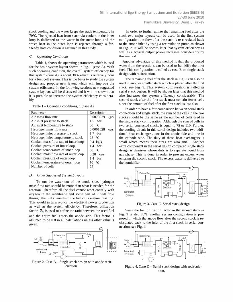
5th International Ege Energy Symposium and Exhibition (IEESE-5) 27-30 June 2010

Pamukkale University, Denizli, Turkey

stack cooling and the water keeps the stack temperature in 70. The rejected heat from stack via coolant in the inner loop is dedicated to the water in the outer loop and the waste heat in the outer loop is rejected through a fan. Steady state condition is assumed in this study.

C. Operating Conditions

Table 1, shows the operating parameters which is used for the basic system layout shown in Fig. 1 (case A). With such operating condition, the overall system efficiency for this system (case A) is about 38% which is relatively poor for a fuel cell system. This is the basis to study the system design and propose new layout which will improve the system efficiency. In the following sections new suggested system layouts will be discussed and it will be shown that it is possible to increase the system efficiency considera-bly.

Table 1 – Operating conditions, 1 (case A)

Parameter Description Air mass flow rate Air inlet pressure to stack Air inlet temperature to stack Hydrogen mass flow rate Hydrogen inlet pressure to stack Hydrogen inlet temperature to stack Coolant mass flow rate of inner loop Coolant pressure of inner loop Coolant temperature of inner loop Coolant mass flow rate of outer loop Coolant pressure of outer loop Coolant temperature of outer loop Number of cells

0.0078929 kg/s 1.5 bar 60 0.0001628 kg/s 1.7 bar 25 0.4 kg/s 1.4 bar 58 0.28 kg/s 1.4 bar 50 75

D. Other Suggested System Layouts

To run the water out of the anode side, hydrogen mass flow rate should be more than what is needed for the reaction. Therefore all the fuel cannot react entirely with oxygen in the membrane and some part of it will flow through the fuel channels of the fuel cells without reacting. This would in turn reduce the electrical power production as well as the system efficiency. Therefore, utilization factor, , is used to define the ratio between the used fuel and the entire fuel enters the anode side. This factor is assumed to be 0.8 in all calculations unless other value is given.

Figure 2. Case B – Single stack design with anode recir-culation.

In order to further utilize the remaining fuel after the stack two major layouts can be used. In the first system configuration the flow after the stack is re-circulated back to the anode inlet by using a recirculation pump as shown in Fig. 2. It will be shown later that system efficiency as well as electrical output power increases considerably by this method.

Another advantage of this method is that the produced water from the reactions can be used to humidify the inlet fuel. This configuration is called as case B or single stack design with recirculation.

The remaining fuel after the stack in Fig. 1 can also be used in another smaller stack which is placed after the first stack, see Fig. 3. This system configuration is called as serial stack design. It will be shown later that this method also increases the system efficiency considerably. The second stack after the first stack must contain fewer cells since the amount of fuel after the first stack is less also.

In order to have a fair comparison between serial stack connection and single stack, the sum of the cells in the two stacks should be the same as the number of cells used in the single stack configuration. Although the sum of cells in two serial connected stacks is equal to 75 or 110. Further, the cooling circuit in this serial design includes two addi-tional heat exchangers, one in the anode side and one in the cathode side. The duty of these heat exchangers is small which means their sizes are also small. Another extra component in the serial design compared single stack design is demister whose duty is to separate liquid from gas phase. This is done in order to prevent excess water entering the second stack. The excess water is delivered to the humidifier.

Figure 3. Case C–Serial stack design

Since the fuel utilization factor in the second stack in Fig. 3 is also 80%, another system configuration is pro-posed in which the anode flow after the second stack is re-circulated back to the inlet of the first stack in serial con-nection, see Fig. 4.

Figure 4, Case D – Serial stack design with recircula-

tion.

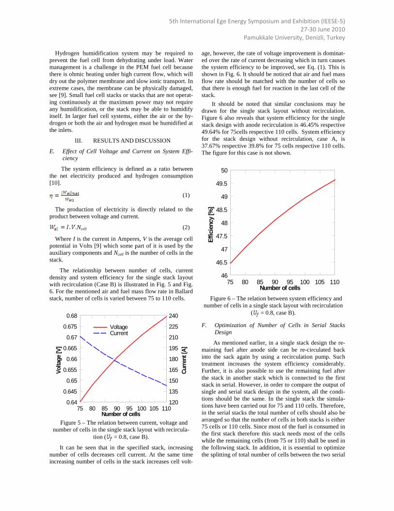
5th International Ege Energy Symposium and Exhibition (IEESE-5) 27-30 June 2010

Pamukkale University, Denizli, Turkey Hydrogen humidification system may be required to

prevent the fuel cell from dehydrating under load. Water management is a challenge in the PEM fuel cell because there is ohmic heating under high current flow, which will dry out the polymer membrane and slow ionic transport. In extreme cases, the membrane can be physically damaged, see [9]. Small fuel cell stacks or stacks that are not operat-ing continuously at the maximum power may not require any humidification, or the stack may be able to humidify itself. In larger fuel cell systems, either the air or the hy-drogen or both the air and hydrogen must be humidified at the inlets.

III. RESULTS AND DISCUSSION

E. Effect of Cell Voltage and Current on System Effi-ciency

The system efficiency is defined as a ratio between the net electricity produced and hydrogen consumption [10].

(1)

The production of electricity is directly related to the product between voltage and current.

.Ncell (2)

Where I is the current in Amperes, V is the average cell potential in Volts [9] which some part of it is used by the auxiliary components and Ncell is the number of cells in the stack.

The relationship between number of cells, current density and system efficiency for the single stack layout with recirculation (Case B) is illustrated in Fig. 5 and Fig. 6. For the mentioned air and fuel mass flow rate in Ballard stack, number of cells is varied between 75 to 110 cells.

Number of cells

Volta

ge [V

]

Curre

nt [A

]

75 80 85 90 95 100 105 1100.64 120

0.645 135

0.65 150

0.655 165

0.66 180

0.665 195

0.67 210

0.675 225

0.68 240

VoltageCurrent

Figure 5 – The relation between current, voltage and

number of cells in the single stack layout with recircula-tion ( = 0.8, case B).

It can be seen that in the specified stack, increasing number of cells decreases cell current. At the same time increasing number of cells in the stack increases cell volt-

age, however, the rate of voltage improvement is dominat-ed over the rate of current decreasing which in turn causes the system efficiency to be improved, see Eq. (1). This is shown in Fig. 6. It should be noticed that air and fuel mass flow rate should be matched with the number of cells so that there is enough fuel for reaction in the last cell of the stack.

It should be noted that similar conclusions may be drawn for the single stack layout without recirculation. Figure 6 also reveals that system efficiency for the single stack design with anode recirculation is 46.45% respective 49.64% for 75cells respective 110 cells. System efficiency for the stack design without recirculation, case A, is 37.67% respective 39.8% for 75 cells respective 110 cells. The figure for this case is not shown.

Number of cells

Effic

ienc

y [%

]

75 80 85 90 95 100 105 11046

46.5

47

47.5

48

48.5

49

49.5

50

Figure 6 – The relation between system efficiency and

number of cells in a single stack layout with recirculation ( = 0.8, case B).

F. Optimization of Number of Cells in Serial Stacks Design

As mentioned earlier, in a single stack design the re-maining fuel after anode side can be re-circulated back into the sack again by using a recirculation pump. Such treatment increases the system efficiency considerably. Further, it is also possible to use the remaining fuel after the stack in another stack which is connected to the first stack in serial. However, in order to compare the output of single and serial stack design in the system, all the condi-tions should be the same. In the single stack the simula-tions have been carried out for 75 and 110 cells. Therefore, in the serial stacks the total number of cells should also be arranged so that the number of cells in both stacks is either 75 cells or 110 cells. Since most of the fuel is consumed in the first stack therefore this stack needs most of the cells while the remaining cells (from 75 or 110) shall be used in the following stack. In addition, it is essential to optimize the splitting of total number of cells between the two serial

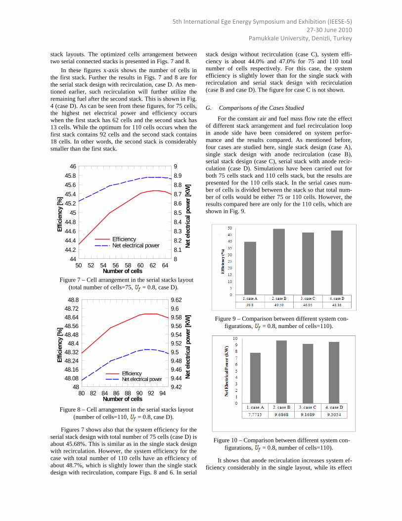
5th International Ege Energy Symposium and Exhibition (IEESE-5) 27-30 June 2010

Pamukkale University, Denizli, Turkey

stack layouts. The optimized cells arrangement between two serial connected stacks is presented in Figs. 7 and 8.

In these figures x-axis shows the number of cells in the first stack. Further the results in Figs. 7 and 8 are for the serial stack design with recirculation, case D. As men-tioned earlier, such recirculation will further utilize the remaining fuel after the second stack. This is shown in Fig. 4 (case D). As can be seen from these figures, for 75 cells, the highest net electrical power and efficiency occurs when the first stack has 62 cells and the second stack has 13 cells. While the optimum for 110 cells occurs when the first stack contains 92 cells and the second stack contains 18 cells. In other words, the second stack is considerably smaller than the first stack.

Number of cells

Effic

ienc

y [%

]

Net e

lect

rical

pow

er [K

W]

50 52 54 56 58 60 62 6444 8

44.2 8.144.4 8.244.6 8.344.8 8.4

45 8.545.2 8.645.4 8.745.6 8.845.8 8.9

46 9

EfficiencyNet electrical power

Figure 7 – Cell arrangement in the serial stacks layout

(total number of cells=75, = 0.8, case D).

Number of cells

Effic

ienc

y [%

]

Net e

lect

rical

pow

er [K

W]

80 82 84 86 88 90 92 9448 9.42

48.08 9.4448.16 9.4648.24 9.4848.32 9.5

48.4 9.5248.48 9.5448.56 9.5648.64 9.5848.72 9.648.8 9.62

EfficiencyNet electrical power

Figure 8 – Cell arrangement in the serial stacks layout

(number of cells=110, = 0.8, case D).

Figures 7 shows also that the system efficiency for the serial stack design with total number of 75 cells (case D) is about 45.68%. This is similar as in the single stack design with recirculation. However, the system efficiency for the case with total number of 110 cells have an efficiency of about 48.7%, which is slightly lower than the single stack design with recirculation, compare Figs. 8 and 6. In serial

stack design without recirculation (case C), system effi-ciency is about 44.0% and 47.0% for 75 and 110 total number of cells respectively. For this case, the system efficiency is slightly lower than for the single stack with recirculation and serial stack design with recirculation (case B and case D). The figure for case C is not shown. G. Comparisons of the Cases Studied

For the constant air and fuel mass flow rate the effect of different stack arrangement and fuel recirculation loop in anode side have been considered on system perfor-mance and the results compared. As mentioned before, four cases are studied here, single stack design (case A), single stack design with anode recirculation (case B), serial stack design (case C), serial stack with anode recir-culation (case D). Simulations have been carried out for both 75 cells stack and 110 cells stack, but the results are presented for the 110 cells stack. In the serial cases num-ber of cells is divided between the stack so that total num-ber of cells would be either 75 or 110 cells. However, the results compared here are only for the 110 cells, which are shown in Fig. 9.

Figure 9 – Comparison between different system con-

figurations, = 0.8, number of cells=110).

Figure 10 – Comparison between different system con-

figurations, = 0.8, number of cells=110).

It shows that anode recirculation increases system ef-ficiency considerably in the single layout, while its effect

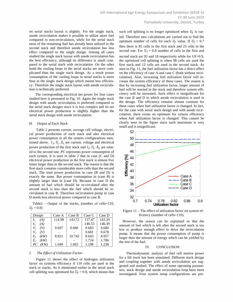
5th International Ege Energy Symposium and Exhibition (IEESE-5) 27-30 June 2010

Pamukkale University, Denizli, Turkey

on serial stacks layout is slightly. For the single stack, anode recirculation makes it possible to utilize more fuel compared to non-recirculation, while for the serial stack most of the remaining fuel has already been utilized in the second stack and therefore anode recirculation has less effect compared to the single design. Among all cases studied the single stack layout with anode recirculation has the best efficiency, although its difference is small com-pared to the serial stack with recirculation. On the other hand the cooling loops in the serial stacks are more com-plicated than the single stack design. As a result power consumption of the cooling loops in serial stacks is more than in the single stack design which means less efficien-cy. Therefore the single stack layout with anode recircula-tion is technically preferred.

The corresponding electrical net power for four cases studied here is presented in Fig. 10. Again the single stack design with anode recirculation is preferred compared to the serial stack designs since it is less complex and its net electrical power production is slightly higher than the serial stack design with anode recirculation.

H. Output of Each Stack

Table 2 presents current, average cell voltage, electri-cal power production of each stack and also electrical power consumption in all the system configurations men-tioned above. are current, voltage and electrical power production of the first stack and are relat-ed to the second one. PC represents power consumption of each system. It is seen in table 2 that in case (C and D) electrical power production in the first stack is almost five times larger than in the second stack. The reason is that the first stack contains considerable more cells than the second stack. The total power production in case (B and D) is exactly the same. But power consumption in (case B) is slightly larger than in (case D). Because in case D the amount of fuel which should be re-circulated after the second stack is less than the fuel which should be re-circulated in case B. Therefore recirculation pump in case D needs less electrical power compared to case B.

Table2 – Output of the stacks, (number of cells=110, = 0.8)

Design Case A Case B Case C Case D I1 (A) I2 (A) V1 (V) V2 (V) E1 (kW) E2 (kW) PC (KW)

114.98 -

0.697 -

8.821 -

1.049

143.72 -

0.680 -

10.743 -

1.065

137.47 140.53 0.683 0.681 8.643 1.724 1.198

143.20 146.39 0.680 0.678 8.957 1.786 1.238

I. The Effect of Utilization Factor:

Figure 11 shows the effect of hydrogen utilization factor on systems efficiency if 110 cells are used in the stack or stacks. As it mentioned earlier in the serial stack cell splitting was optimized for = 0.8, which means that

such cell splitting is no longer optimized when is var-ied. Therefore new calculations are carried out to find the optimum number of cells for each value. If = 0.7 then there is 85 cells in the first stack and 25 cells in the second one. For = 0.8 number of cells in the first and second stack are 92 and 18 respectively while for UF=0.9, the optimized cell splitting is when 98 cells are used the first stack and 12 cells are used in the second stack. As seen in Fig. 11, the fuel utilization factor has a direct effect on the efficiency of case A and case C (both without recir-culation). Also, increasing fuel utilization factor will in-crease the system efficiency of these cases. The reason is that by increasing fuel utilization factor, larger amount of fuel will be reacted in the stack and therefore system effi-ciency will be increased. Such effect is insignificant for the case B and D in which anode recirculation is used in the design. The efficiency remains almost constant for these cases when fuel utilization factor is changed. In fact, for the case with serial stack design and with anode recir-culation, there exists an optimum for system efficiency when fuel utilization factor is changed. This cannot be clearly seen in the figure since such maximum is very small and is insignificant.

Utilization factor

Effic

ienc

y [%

]

0.7 0.74 0.78 0.82 0.86 0.932

34

36

38

40

42

44

46

48

50

52

Case ACase BCase CCase D

Figure 11 – The effect of utilization factor on system ef-

ficiency (number of cells=110).

However, the reason can be explained so that the amount of fuel which is left after the second stack is too low to produce enough effect to drive the recirculation pump. It means that the power consumption of pump is larger than the amount of energy which can be yielded by the rest of the fuel.

IV. CONCLUSION

Thermodynamic analysis of fuel cell motive power for a lift truck has been simulated. Different stack design and coupling together with anode recirculation are sug-gested and studied. The effect of some operating parame-ters, stack design and anode recirculation loop have been investigated. Four system setup configurations are pre-

5th International Ege Energy Symposium and Exhibition (IEESE-5) 27-30 June 2010

Pamukkale University, Denizli, Turkey

sented. These are listed as single stack without recircula-tion (case A), single stack with recirculation (case B), serial stack without recirculation (case C) and serial stack with recirculation (case D). The calculations have been carried out for two sets of cell numbers which are equal to 75 and 110 cells. For 75 number of cells the efficiency in the basic case (case A) is 34% which is quite low. In this paper various approaches for efficiency improvement have been studied to reach system efficiencies of about 50%. The results show that in constant operating conditions increasing the number of cells increase the efficiency. Anode recirculation loop increases the efficiency in both single and serial stack design, but its effect is much larger in the single stack compared serial stack design. For 110 number of cells and = 0.8 efficiency improvement due to anode recirculation is about 10% for single stack com-pared to about 2% in serial stack design. Another issue which is discussed in this paper is about cell arrangement. It is found that without recirculation loop, serial stack design has a higher efficiency compared single stack, around 7% higher. However, for the systems with anode recirculation, (case B and case D) the efficiency of the single stack design is about 1% higher than the serial stack layout. Therefore single stack with recirculation (case B) is proposed as the most efficient fuel cell system because of its high efficiency and simplicity.

REFERENCES

[1] WWW.BALLARD.COM [2] Boettner, D.D.; and Moran, M.J. 2004. Proton ex-

change membrane (PEM) fuel cell-powered vehicle performance using direct-hydrogen fueling and on-board methanol reforming. Energy 29(12-15): 2317–2330.

[3] Yuan, J.; Rokni, M.; and Sundén, B. 2003. A numeri-cal investigation of gas flow and heat transfer in pro-ton exchange membrane fuel cells. Num. Heat Trans-fer, part A 44(3): 255–280.

[4] Yu, X.; Zhou, B.; and Sobiesiak, A. 2005. Water and thermal management for Ballard PEM fuel cell stack. Journal of Power Sources 147(1-2): 184–195.

[5] Seddiq, M.; Khaleghi, H.; and Mirzaei,M. 2006. Nu-merical analysis of gas cross-over through the mem-brane in a proton exchange membrane fuel cell. Jour-nal of Power Sources 161(1): 371–379.

[6] Ogden, J.M.; Steinbugler, M.M.; and Kreutz. T.G. 1998. A comparison of hydrogen, methanol and gaso-line as fuels for fuel cell vehicles: implications for ve-hicle design and infrastructure development. Journal of Power Sources 79(2): 143–168.

[7] Kima, S.C.; Wona, J.P.; Parkb, Y.S.; Limb, T.W.; and Kim, M.S. 2009. Performance evaluation of a stack cooling system using CO2 air conditioner in fuel cell vehicles. International journal of refrigeration 32(2009): 70 –77.

[8] Ahluwalia, R.K.; and Wang. X. 2005. Direct hydro-gen fuel cell systems for hybrid vehicles. Journal of Power Sources. 139(1): 152–164.

[9] Spiegel, C. 2007. Designing and building fuel cells. McGraw-Hill, Two Penn Plaza, New York.

[10] Spiegel, C. 2008. PEM fuel cell modeling and simula-tion using Matlab. Printed in the United States of America.

BIOGRAPHIES

Elham Hosseinzadeh – was born in 1984. She received her master of science in 2008 with thesis topic on experi-mental study of a radiative cooling system with flat plate solar collectors from Babol University of technology in Iran. She is doing her PhD on the project, fuel cell hydro-gen manifold for lift trucks in DTU (Technical University of Denmark).

Masoud Rokni – was born on 1962. He received his master of science in 1992 with thesis topic on combination of a solid oxide fuel cell and combined cycles from Lund University in Sweden. He received his doctoral degree in 1998 from Lund University in Sweden on heat transfer and fluid flow. In 2002 he was appointed as Docent at the same university.

He has published more than 20 journal manuscript on fuel based power plants and fluid flow and heat transfer on channels of different application area such as fuel cells and heat exchangers. He has also contributed more than 30 conference articles on power plants, fuels cells and fluid flow and heat transfer and turbulence modeling. His cur-rent research area is about designing of fuel cells system for power generating such as PEMFC for automotive vehi-cles and SOFC based power plants. He has also written more than 20 internal reports.

Dr. Rokni is the member of Hydrogen Link associa-tion in Denmark, reviewer of several international jour-nals, member of DCMC, ASME, etc. Among others Dr. Rokni has also worked as System Manger at Wärtsilä Corporation on building SOFC based power plants.

Appendix G

Paper VI

Application of Proton Exchange Membrane Fuel Cell for Lift Trucks

223

European Fuel Cell Forum 2011 28 June -1 July 2011, Lucerne Switzerland

A1403 / Page 1-11

A1403

Application of Proton Exchange Membrane Fuel Cell for Lift Trucks

Elham Hosseinzadeh and Masoud Rokni

Technical University of Denmark (DTU) Dept. of Mechanical Engineering, Thermal Energy Section

Building 403, Room 111 2800 Kgs, Lyngby Tel.: +45-45254161 Fax: +45-45935215

ehos@mek.dtu.dk

Abstract In this study a general PEMFC (Proton Exchange Membrane Fuel Cell) model has been developed to take into account the effect of pressure losses, water crossovers, humidity aspects and voltage over potentials in the cells. The model is zero dimensional and it is assumed to be steady state. The effect of concentration loss is neglected while the effect of activation and ohmic losses is investigated in the system. Some semi-empirical equations are required to predict the amount of exchange current density for calculation of ohmic loss and water diffusion coefficient through membrane. These equations are applied in order to account for water back diffusion. Further Membrane water content is assumed to be a linear function of thickness. PEM fuel cell is working at rather low operating conditions which makes it suitable for the automotive systems. In this paper motive power part of a lift truck has been investigated thermodynamically. The system includes a compressor, an air humidifier, set of heat exchangers and a stack which together build up the anode circuit, the cathode circuit and the cooling loop. Since fuel humidification is carried out via water cross over from cathode to anode, there is no humidifier in the anode side. The electricity needed for auxiliary components is produced by the stack. The system is set at different electrical powers. In this paper several issues are discussed; voltage losses, system efficiency as well as electrical power at different operating conditions. Key words: PEMFC, fuel cell, anode recirculation, ohmic loss, activation loss, concentration loss, exchange current density, back diffusion

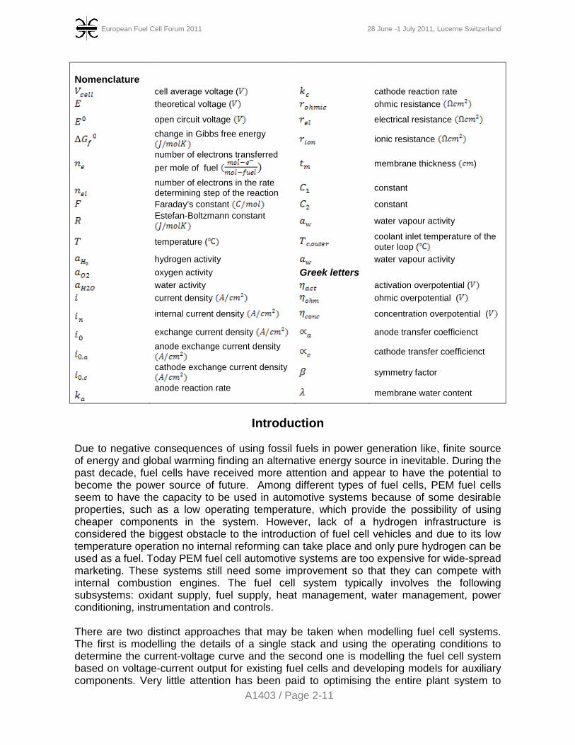
European Fuel Cell Forum 2011 28 June -1 July 2011, Lucerne Switzerland

A1403 / Page 2-11

Nomenclature

cell average voltage ( cathode reaction rate

theoretical voltage ( ohmic resistance

open circuit voltage electrical resistance

change in Gibbs free energy

ionic resistance

number of electrons transferred per mole of fuel membrane thickness )

number of electrons in the rate determining step of the reaction constant

Faraday’s constant constant

Estefan-Boltzmann constant

water vapour activity

temperature ( coolant inlet temperature of the outer loop (

hydrogen activity water vapour activity oxygen activity Greek letters

water activity activation overpotential ( current density ohmic overpotential (

internal current density concentration overpotential (

exchange current density anode transfer coefficienct

anode exchange current density

cathode transfer coefficienct

cathode exchange current density

symmetry factor

anode reaction rate membrane water content

Introduction

Due to negative consequences of using fossil fuels in power generation like, finite source of energy and global warming finding an alternative energy source in inevitable. During the past decade, fuel cells have received more attention and appear to have the potential to become the power source of future. Among different types of fuel cells, PEM fuel cells seem to have the capacity to be used in automotive systems because of some desirable properties, such as a low operating temperature, which provide the possibility of using cheaper components in the system. However, lack of a hydrogen infrastructure is considered the biggest obstacle to the introduction of fuel cell vehicles and due to its low temperature operation no internal reforming can take place and only pure hydrogen can be used as a fuel. Today PEM fuel cell automotive systems are too expensive for wide-spread marketing. These systems still need some improvement so that they can compete with internal combustion engines. The fuel cell system typically involves the following subsystems: oxidant supply, fuel supply, heat management, water management, power conditioning, instrumentation and controls. There are two distinct approaches that may be taken when modelling fuel cell systems. The first is modelling the details of a single stack and using the operating conditions to determine the current-voltage curve and the second one is modelling the fuel cell system based on voltage-current output for existing fuel cells and developing models for auxiliary components. Very little attention has been paid to optimising the entire plant system to

European Fuel Cell Forum 2011 28 June -1 July 2011, Lucerne Switzerland

A1403 / Page 3-11

make the fuel cell system work efficiently. In order to have a comprehensive understanding of a fuel cell, one needs to look at its operation in the system. Modelling a fuel cell stack alone is not very advantageous. In order to investigate and optimise a fuel cell system, it is necessary to develop a comprehensive model of the stack. There are many articles in the literature which have focused on numerical modelling of the stack and the detailed phenomena which occur in it. Papers [1] to [4] developed mathematical models based on analytical approaches. Papers [5] and [6] provide a discussion of the polarization curve in PEMFC. In [7] some key parameters estimation for the polarization curve was proposed. Other papers have discussed electrolyte properties and water diffusion phenomena in the stack. In [8] a transient analysis of water transport in a PEM fuel cell was studied in theory. In [9] an isothermal, one-dimensional, steady-state model for PEMFC was presented with a 117 Nafion as a membrane. Other researchers have taken the second approach, incorporating PEM fuel cell voltage–current density curves for existing fuel cells into a system model to examine fuel cell system performance in automotive applications [10]–[12]. In this paper a simple but general model for PEMFC is developed, which is zero dimensional and steady state. The polarization curve of the stack captures the experimental data very well. The model is applied to a 14 kw fork-lift truck power system. The thermodynamic efficiency and net power of the system is calculated for different operating conditions. The results are then validated against experimental data.

1. Methodology In this study the thermodynamic analysis of PEMFC for a fuel cell automotive system was investigated. The conditions were assumed to be steady-state. A zero-dimensional PEMFC model was developed and is presented here. This model was built up in an in-house software, called DNA (dynamic network analysis), which is FORTRAN based. The equations used for modelling were either analytical or semi-empirical and were taken from the literature. The accuracy of the theoretical results was validated against experimental data and the I-V curve produced by this model fit very well with the corresponding experimental data. The fuel cell stack contains 110 cells with the cell area equal to 285.88

The operating temperature of the stack was 60-80 and the maximum power which could be produced was equal to 20.4 kw. The advantage of this model is that it can be used for all types of PEMFC stacks by replacing some parameters, as explained in detail in the following sections.

2. System description Figure 1, shows the schematic of the fuel cell system analysed in this study. The system includes a compressor, an air humidifier, a set of heat exchangers and a stack, which together build up the cathode circuit, the anode circuit and the cooling loop. On the cathode side, air is compressed, pre-cooled and humidified before entering the cathode side of the stack at a pressure less than 2 bar and a temperature around 60 . The fuel used on the anode side is pure hydrogen which is assumed to be pressurized and stored in a vessel. The amount of hydrogen will be regulated by using a valve just after the vessel. For the sake of simplicity this valve is not shown in the figure. Hydrogen with a pressure less than 2.2 bar and temperature around 60 enters the anode side of the

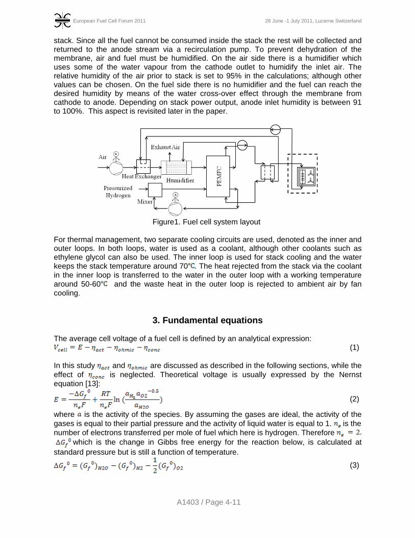
European Fuel Cell Forum 2011 28 June -1 July 2011, Lucerne Switzerland

A1403 / Page 4-11

stack. Since all the fuel cannot be consumed inside the stack the rest will be collected and returned to the anode stream via a recirculation pump. To prevent dehydration of the membrane, air and fuel must be humidified. On the air side there is a humidifier which uses some of the water vapour from the cathode outlet to humidify the inlet air. The relative humidity of the air prior to stack is set to 95% in the calculations; although other values can be chosen. On the fuel side there is no humidifier and the fuel can reach the desired humidity by means of the water cross-over effect through the membrane from cathode to anode. Depending on stack power output, anode inlet humidity is between 91 to 100%. This aspect is revisited later in the paper.

Figure1. Fuel cell system layout

For thermal management, two separate cooling circuits are used, denoted as the inner and outer loops. In both loops, water is used as a coolant, although other coolants such as ethylene glycol can also be used. The inner loop is used for stack cooling and the water keeps the stack temperature around 70 . The heat rejected from the stack via the coolant in the inner loop is transferred to the water in the outer loop with a working temperature around 50-60 and the waste heat in the outer loop is rejected to ambient air by fan cooling.

3. Fundamental equations The average cell voltage of a fuel cell is defined by an analytical expression:

(1) In this study and are discussed as described in the following sections, while the effect of is neglected. Theoretical voltage is usually expressed by the Nernst equation [13]:

(2)

where is the activity of the species. By assuming the gases are ideal, the activity of the gases is equal to their partial pressure and the activity of liquid water is equal to 1. is the number of electrons transferred per mole of fuel which here is hydrogen. Therefore

which is the change in Gibbs free energy for the reaction below, is calculated at standard pressure but is still a function of temperature.

(3)

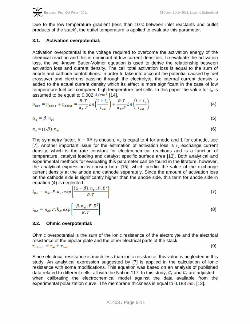
European Fuel Cell Forum 2011 28 June -1 July 2011, Lucerne Switzerland

A1403 / Page 5-11

Due to the low temperature gradient (less than 10 between inlet reactants and outlet products of the stack), the outlet temperature is applied to evaluate this parameter. 3.1. Activation overpotential: Activation overpotential is the voltage required to overcome the activation energy of the chemical reaction and this is dominant at low current densities. To evaluate the activation loss, the well-known Butler-Volmer equation is used to derive the relationship between activation loss and current density. The cell total activation loss is equal to the sum of anode and cathode contributions. In order to take into account the potential caused by fuel crossover and electrons passing through the electrolyte, the internal current density is added to the actual current density which its effect is more significant in the case of low temperature fuel cell compared high temperature fuel cells. In this paper the value for is assumed to be equal to 0.002 [14].

(4)

(5)

= (1- (6)

The symmetry factor, is chosen, is equal to 4 for anode and 1 for cathode, see [7]. Another important issue for the estimation of activation loss is exchange current density, which is the rate constant for electrochemical reactions and is a function of temperature, catalyst loading and catalyst specific surface area [13]. Both analytical and experimental methods for evaluating this parameter can be found in the litrature. however, the analytical expression is chosen here [15], which predict the value of the exchange current density at the anode and cathode separately. Since the amount of activation loss on the cathode side is significantly higher than the anode side, this term for anode side in equation (4) is neglected.

(7)

(8)

3.2. Ohmic overpotential: Ohmic overpotential is the sum of the ionic resistance of the electrolyte and the electrical resistance of the bipolar plate and the other electrical parts of the stack.

(9) Since electrical resistance is much less than ionic resistance, this value is neglected in this study. An analytical expression suggested by [7] is applied in the calculation of ionic resistance with some modifications. This equation was based on an analysis of published data related to different cells, all with the Nafion 117. In this study, and are adjusted when calibrating the electrochemical model against the data available from the experimental polarization curve. The membrane thickness is equal to 0.183 [13].

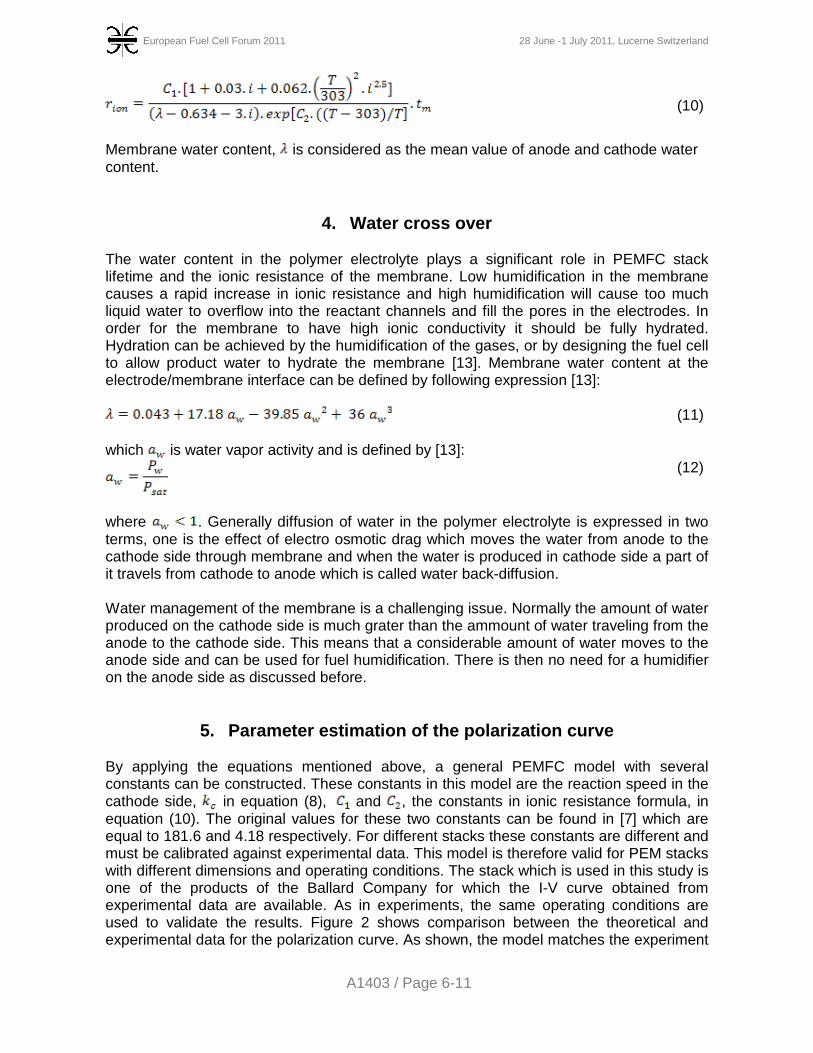
European Fuel Cell Forum 2011 28 June -1 July 2011, Lucerne Switzerland

A1403 / Page 6-11

(10)

Membrane water content, is considered as the mean value of anode and cathode water content.

4. Water cross over

The water content in the polymer electrolyte plays a significant role in PEMFC stack lifetime and the ionic resistance of the membrane. Low humidification in the membrane causes a rapid increase in ionic resistance and high humidification will cause too much liquid water to overflow into the reactant channels and fill the pores in the electrodes. In order for the membrane to have high ionic conductivity it should be fully hydrated. Hydration can be achieved by the humidification of the gases, or by designing the fuel cell to allow product water to hydrate the membrane [13]. Membrane water content at the electrode/membrane interface can be defined by following expression [13]:

(11)

which is water vapor activity and is defined by [13]:

(12)

where . Generally diffusion of water in the polymer electrolyte is expressed in two terms, one is the effect of electro osmotic drag which moves the water from anode to the cathode side through membrane and when the water is produced in cathode side a part of it travels from cathode to anode which is called water back-diffusion. Water management of the membrane is a challenging issue. Normally the amount of water produced on the cathode side is much grater than the ammount of water traveling from the anode to the cathode side. This means that a considerable amount of water moves to the anode side and can be used for fuel humidification. There is then no need for a humidifier on the anode side as discussed before.

5. Parameter estimation of the polarization curve By applying the equations mentioned above, a general PEMFC model with several constants can be constructed. These constants in this model are the reaction speed in the cathode side, in equation (8), and , the constants in ionic resistance formula, in equation (10). The original values for these two constants can be found in [7] which are equal to 181.6 and 4.18 respectively. For different stacks these constants are different and must be calibrated against experimental data. This model is therefore valid for PEM stacks with different dimensions and operating conditions. The stack which is used in this study is one of the products of the Ballard Company for which the I-V curve obtained from experimental data are available. As in experiments, the same operating conditions are used to validate the results. Figure 2 shows comparison between the theoretical and experimental data for the polarization curve. As shown, the model matches the experiment

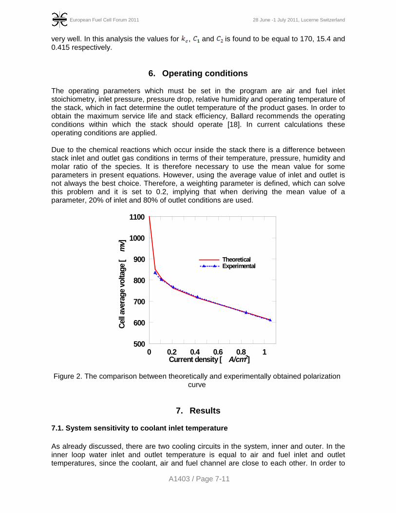
European Fuel Cell Forum 2011 28 June -1 July 2011, Lucerne Switzerland

A1403 / Page 7-11

very well. In this analysis the values for , and is found to be equal to 170, 15.4 and 0.415 respectively.

6. Operating conditions The operating parameters which must be set in the program are air and fuel inlet stoichiometry, inlet pressure, pressure drop, relative humidity and operating temperature of the stack, which in fact determine the outlet temperature of the product gases. In order to obtain the maximum service life and stack efficiency, Ballard recommends the operating conditions within which the stack should operate [18]. In current calculations these operating conditions are applied. Due to the chemical reactions which occur inside the stack there is a difference between stack inlet and outlet gas conditions in terms of their temperature, pressure, humidity and molar ratio of the species. It is therefore necessary to use the mean value for some parameters in present equations. However, using the average value of inlet and outlet is not always the best choice. Therefore, a weighting parameter is defined, which can solve this problem and it is set to 0.2, implying that when deriving the mean value of a parameter, 20% of inlet and 80% of outlet conditions are used.

Current density [ A/cm2]

Cell a

vera

ge v

olta

ge [

mv]

0 0.2 0.4 0.6 0.8 1500

600

700

800

900

1000

1100

TheoreticalExperimental

Figure 2. The comparison between theoretically and experimentally obtained polarization curve

7. Results 7.1. System sensitivity to coolant inlet temperature As already discussed, there are two cooling circuits in the system, inner and outer. In the inner loop water inlet and outlet temperature is equal to air and fuel inlet and outlet temperatures, since the coolant, air and fuel channel are close to each other. In order to

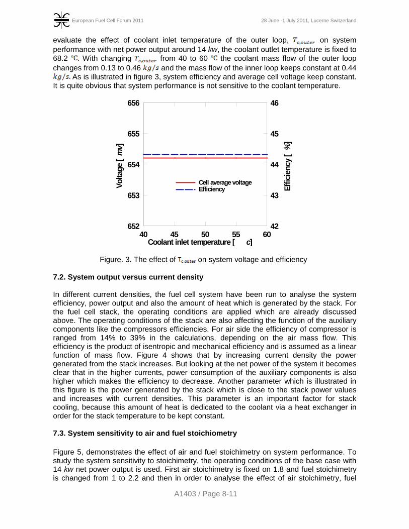
European Fuel Cell Forum 2011 28 June -1 July 2011, Lucerne Switzerland

A1403 / Page 8-11

evaluate the effect of coolant inlet temperature of the outer loop, on system performance with net power output around 14 kw, the coolant outlet temperature is fixed to 68.2 . With changing from 40 to 60 the coolant mass flow of the outer loop changes from 0.13 to 0.46 and the mass flow of the inner loop keeps constant at 0.44

As is illustrated in figure 3, system efficiency and average cell voltage keep constant. It is quite obvious that system performance is not sensitive to the coolant temperature.

Coolant inlet temperature [ c]

Volta

ge [

mv]

Effic

ienc

y [

%]

40 45 50 55 60652 42

653 43

654 44

655 45

656 46

Cell average voltageEfficiency

Figure. 3. The effect of on system voltage and efficiency

7.2. System output versus current density

In different current densities, the fuel cell system have been run to analyse the system efficiency, power output and also the amount of heat which is generated by the stack. For the fuel cell stack, the operating conditions are applied which are already discussed above. The operating conditions of the stack are also affecting the function of the auxiliary components like the compressors efficiencies. For air side the efficiency of compressor is ranged from 14% to 39% in the calculations, depending on the air mass flow. This efficiency is the product of isentropic and mechanical efficiency and is assumed as a linear function of mass flow. Figure 4 shows that by increasing current density the power generated from the stack increases. But looking at the net power of the system it becomes clear that in the higher currents, power consumption of the auxiliary components is also higher which makes the efficiency to decrease. Another parameter which is illustrated in this figure is the power generated by the stack which is close to the stack power values and increases with current densities. This parameter is an important factor for stack cooling, because this amount of heat is dedicated to the coolant via a heat exchanger in order for the stack temperature to be kept constant.

7.3. System sensitivity to air and fuel stoichiometry Figure 5, demonstrates the effect of air and fuel stoichimetry on system performance. To study the system sensitivity to stoichimetry, the operating conditions of the base case with 14 kw net power output is used. First air stoichimetry is fixed on 1.8 and fuel stoichimetry is changed from 1 to 2.2 and then in order to analyse the effect of air stoichimetry, fuel

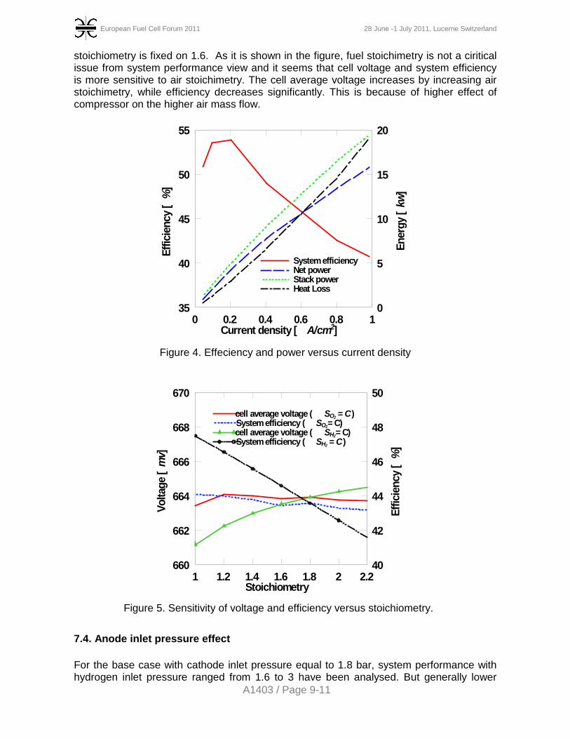
European Fuel Cell Forum 2011 28 June -1 July 2011, Lucerne Switzerland

A1403 / Page 9-11

stoichiometry is fixed on 1.6. As it is shown in the figure, fuel stoichimetry is not a ciritical issue from system performance view and it seems that cell voltage and system efficiency is more sensitive to air stoichimetry. The cell average voltage increases by increasing air stoichimetry, while efficiency decreases significantly. This is because of higher effect of compressor on the higher air mass flow.

Current density [ A/cm2]

Effic

ienc

y [

%]

Ener

gy [

kw]

0 0.2 0.4 0.6 0.8 135 0

40 5

45 10

50 15

55 20

System efficiencyNet powerStack powerHeat Loss

Figure 4. Effeciency and power versus current density

Stoichiometry

Volta

ge [

mv]

Effic

ienc

y [

%]

1 1.2 1.4 1.6 1.8 2 2.2660 40

662 42

664 44

666 46

668 48

670 50

cell average voltage ( SO2 = C)System efficiency ( SO2 = C)cell average voltage ( SH2 = C)System efficiency ( SH2 = C)

Figure 5. Sensitivity of voltage and efficiency versus stoichiometry.

7.4. Anode inlet pressure effect For the base case with cathode inlet pressure equal to 1.8 bar, system performance with hydrogen inlet pressure ranged from 1.6 to 3 have been analysed. But generally lower

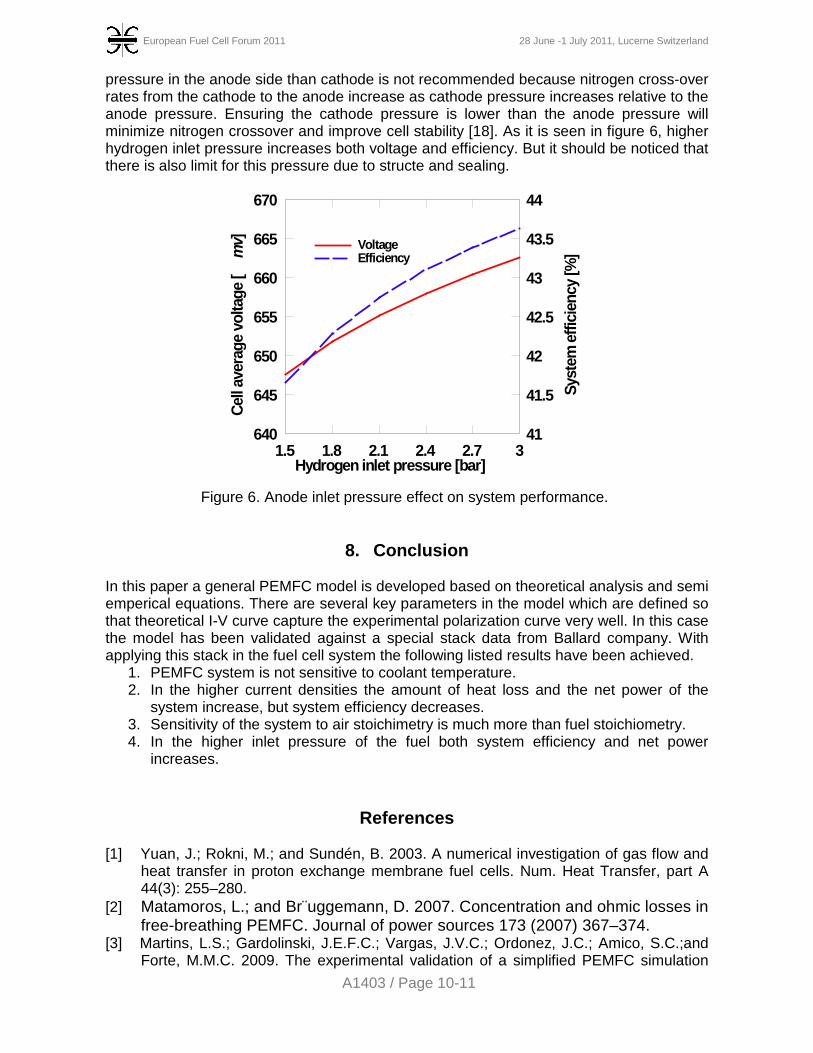
European Fuel Cell Forum 2011 28 June -1 July 2011, Lucerne Switzerland

A1403 / Page 10-11

pressure in the anode side than cathode is not recommended because nitrogen cross-over rates from the cathode to the anode increase as cathode pressure increases relative to the anode pressure. Ensuring the cathode pressure is lower than the anode pressure will minimize nitrogen crossover and improve cell stability [18]. As it is seen in figure 6, higher hydrogen inlet pressure increases both voltage and efficiency. But it should be noticed that there is also limit for this pressure due to structe and sealing.

Hydrogen inlet pressure [bar]

Cell a

vera

ge v

olta

ge [

mv]

Syst

em e

ffici

ency

[%]

1.5 1.8 2.1 2.4 2.7 3640 41

645 41.5

650 42

655 42.5

660 43

665 43.5

670 44

VoltageEfficiency

Figure 6. Anode inlet pressure effect on system performance.

8. Conclusion

In this paper a general PEMFC model is developed based on theoretical analysis and semi emperical equations. There are several key parameters in the model which are defined so that theoretical I-V curve capture the experimental polarization curve very well. In this case the model has been validated against a special stack data from Ballard company. With applying this stack in the fuel cell system the following listed results have been achieved.

1. PEMFC system is not sensitive to coolant temperature. 2. In the higher current densities the amount of heat loss and the net power of the

system increase, but system efficiency decreases. 3. Sensitivity of the system to air stoichimetry is much more than fuel stoichiometry. 4. In the higher inlet pressure of the fuel both system efficiency and net power

increases.

References [1] Yuan, J.; Rokni, M.; and Sundén, B. 2003. A numerical investigation of gas flow and

heat transfer in proton exchange membrane fuel cells. Num. Heat Transfer, part A 44(3): 255–280.

[2] Matamoros, L.; and Br¨uggemann, D. 2007. Concentration and ohmic losses in free-breathing PEMFC. Journal of power sources 173 (2007) 367–374.

[3] Martins, L.S.; Gardolinski, J.E.F.C.; Vargas, J.V.C.; Ordonez, J.C.; Amico, S.C.;and Forte, M.M.C. 2009. The experimental validation of a simplified PEMFC simulation

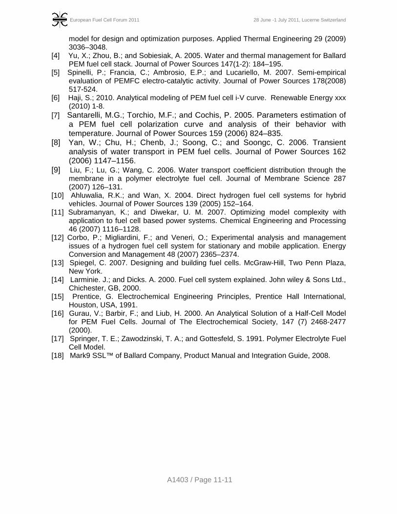
European Fuel Cell Forum 2011 28 June -1 July 2011, Lucerne Switzerland

A1403 / Page 11-11

model for design and optimization purposes. Applied Thermal Engineering 29 (2009) 3036–3048.

[4] Yu, X.; Zhou, B.; and Sobiesiak, A. 2005. Water and thermal management for Ballard PEM fuel cell stack. Journal of Power Sources 147(1-2): 184–195.

[5] Spinelli, P.; Francia, C.; Ambrosio, E.P.; and Lucariello, M. 2007. Semi-empirical evaluation of PEMFC electro-catalytic activity. Journal of Power Sources 178(2008) 517-524.

[6] Haji, S.; 2010. Analytical modeling of PEM fuel cell i-V curve. Renewable Energy xxx (2010) 1-8.

[7] Santarelli, M.G.; Torchio, M.F.; and Cochis, P. 2005. Parameters estimation of a PEM fuel cell polarization curve and analysis of their behavior with temperature. Journal of Power Sources 159 (2006) 824–835.

[8] Yan, W.; Chu, H.; Chenb, J.; Soong, C.; and Soongc, C. 2006. Transient analysis of water transport in PEM fuel cells. Journal of Power Sources 162 (2006) 1147–1156.

[9] Liu, F.; Lu, G.; Wang, C. 2006. Water transport coefficient distribution through the membrane in a polymer electrolyte fuel cell. Journal of Membrane Science 287 (2007) 126–131.

[10] Ahluwalia, R.K.; and Wan, X. 2004. Direct hydrogen fuel cell systems for hybrid vehicles. Journal of Power Sources 139 (2005) 152–164.

[11] Subramanyan, K.; and Diwekar, U. M. 2007. Optimizing model complexity with application to fuel cell based power systems. Chemical Engineering and Processing 46 (2007) 1116–1128.

[12] Corbo, P.; Migliardini, F.; and Veneri, O.; Experimental analysis and management issues of a hydrogen fuel cell system for stationary and mobile application. Energy Conversion and Management 48 (2007) 2365–2374.

[13] Spiegel, C. 2007. Designing and building fuel cells. McGraw-Hill, Two Penn Plaza, New York.

[14] Larminie. J.; and Dicks. A. 2000. Fuel cell system explained. John wiley & Sons Ltd., Chichester, GB, 2000.

[15] Prentice, G. Electrochemical Engineering Principles, Prentice Hall International, Houston, USA, 1991.

[16] Gurau, V.; Barbir, F.; and Liub, H. 2000. An Analytical Solution of a Half-Cell Model for PEM Fuel Cells. Journal of The Electrochemical Society, 147 (7) 2468-2477 (2000).

[17] Springer, T. E.; Zawodzinski, T. A.; and Gottesfeld, S. 1991. Polymer Electrolyte Fuel Cell Model.

[18] Mark9 SSL™ of Ballard Company, Product Manual and Integration Guide, 2008.