Modeling and Control of Flapping Wing Robots · Masters of Science in Mechanical Engineering Andrew...
79
Modeling and Control of Flapping Wing Robots Ian P. Murphy Thesis submitted to the Faculty of the Virginia Polytechnic Institute and State University in partial fulfilment of the requirements for the degree of Masters of Science in Mechanical Engineering Andrew J. Kurdila, Co-Chair Javid Bayandor, Co-Chair Ricardo A. Burdisso February 8, 2013 Blacksburg, Virginia Keywords: Flapping Flight, Robotic Modeling, Nonlinear Control, Adaptive Control Copyright 2013, Ian P. Murphy
Transcript of Modeling and Control of Flapping Wing Robots · Masters of Science in Mechanical Engineering Andrew...

Modeling and Control of Flapping Wing Robots
Ian P. Murphy
Thesis submitted to the Faculty of theVirginia Polytechnic Institute and State University
in partial fulfilment of the requirements for the degree of
Masters of Sciencein
Mechanical Engineering
Andrew J. Kurdila, Co-ChairJavid Bayandor, Co-Chair
Ricardo A. Burdisso
February 8, 2013Blacksburg, Virginia
Keywords: Flapping Flight, Robotic Modeling, Nonlinear Control, Adaptive ControlCopyright 2013, Ian P. Murphy

Modeling and Control of Flapping Wing Robots
Ian P. Murphy
(ABSTRACT)
The study of fixed wing aeronautical engineering has matured to the point where years of researchresult in small performance improvements. In the past decade, micro air vehicles, or MAVs, havegained attention of the aerospace and robotics communities. Many researchers have begun investi-gating aircraft schemes such as ones which use rotary or flapping wings for propulsion. While theengineering of rotary wing aircraft has seen significant advancement, the complex physics behindflapping wing aircraft remains to be fully understood. Some studies suggest flapping wing aircraftcan be more efficient when the aircraft operates in low Reynolds regimes or requires hovering. Be-cause of this inherent complexity, the derivation of flapping wing control methodologies remainsan area with many open research problems. This thesis investigates flapping wing vehicles whosedesign is inspired by avian flight. The flapping wing system is examined in the cases where thecore body is fixed or free in the ground frame. When the core body is fixed, the Denavit Harten-berg representation is used for the kinematic variables. An alternative approach is introduced fora free base body case. The equations of motion are developed using Lagranges equations and aprocess is developed to derive the aerodynamic contributions using a virtual work principle. Theaerodynamics are modeled using a quasi-steady state formulation where the lift and drag coeffi-cients are treated as unknowns. A collection of nonlinear controllers are studied, specifically anideal dynamic inversion controller and two switching dynamic inversion controllers. A dynamicinversion controller is modified with an adaptive term that learns the aerodynamic effects on theequation of motion. The dissipative controller with adaptation is developed to improve perfor-mance. A Lyapunov analysis of the two adaptive controllers guarantees boundedness for all errorterms. Asymptotic stability is guaranteed for the derivative error in the dynamic inversion con-troller and for both the position and derivative error in the dissipative controller. The controllersare simulated using two dynamic models based on flapping wing prototypes designed at VirginiaTech. The numerical experiments validate the Lyapunov analysis and illustrate that unknown pa-rameters can be learned if persistently excited.
This work received support through contract JFC-11-139 as part of the Institute for Critical Tech-nology and Applied Science (ICTAS).

Contents
1 Introduction and Motivation 1
1.1 Literature Review . . . . . . . . . . . . . . . . . . . . . . . . . . . . . . . . . . . 2
1.2 Nomenclature List . . . . . . . . . . . . . . . . . . . . . . . . . . . . . . . . . . 7
2 Dynamic Models of Flapping Wing Robots 8
2.1 Review of Robot Kinematics . . . . . . . . . . . . . . . . . . . . . . . . . . . . . 8
2.1.1 Rotation Matrices . . . . . . . . . . . . . . . . . . . . . . . . . . . . . . . 8
2.1.2 Homogeneous Transforms . . . . . . . . . . . . . . . . . . . . . . . . . . 9
2.1.3 Denavit-Hartenberg Convention . . . . . . . . . . . . . . . . . . . . . . . 11
2.1.4 Angular Velocity and Translational Velocity . . . . . . . . . . . . . . . . . 12
2.2 Lagrange’s Equations . . . . . . . . . . . . . . . . . . . . . . . . . . . . . . . . . 14
2.2.1 Fixed Base Body . . . . . . . . . . . . . . . . . . . . . . . . . . . . . . . 15
2.2.2 Moving Base Body . . . . . . . . . . . . . . . . . . . . . . . . . . . . . . 16
2.3 Aerodynamic Model . . . . . . . . . . . . . . . . . . . . . . . . . . . . . . . . . 21
2.4 Examples of Dynamic and Kinematic Models . . . . . . . . . . . . . . . . . . . . 25
3 Control of Flapping Wing Robots 31
3.1 Approximate Dynamic Inversion . . . . . . . . . . . . . . . . . . . . . . . . . . . 31
3.1.1 Hard Switching Controller . . . . . . . . . . . . . . . . . . . . . . . . . . 32
3.1.2 Soft Switching Controller . . . . . . . . . . . . . . . . . . . . . . . . . . 34
3.2 Adaptive Control . . . . . . . . . . . . . . . . . . . . . . . . . . . . . . . . . . . 34
3.2.1 Approximate Dynamic Inversion with Adaptation . . . . . . . . . . . . . . 34
iii

3.2.2 Dissipative Controller with Adaptation . . . . . . . . . . . . . . . . . . . 36
3.3 Numerical Simulation . . . . . . . . . . . . . . . . . . . . . . . . . . . . . . . . . 37
3.3.1 Software Architecture . . . . . . . . . . . . . . . . . . . . . . . . . . . . 37
3.3.2 Dynamic Inversion Controller . . . . . . . . . . . . . . . . . . . . . . . . 40
3.3.3 Dissipative Controller . . . . . . . . . . . . . . . . . . . . . . . . . . . . 51
4 Conclusion 58
4.1 Future Work . . . . . . . . . . . . . . . . . . . . . . . . . . . . . . . . . . . . . . 59
A Dynamic Model Examples 63
A.1 Daedalus Mass Matrix . . . . . . . . . . . . . . . . . . . . . . . . . . . . . . . . 63
A.2 Daedalus Nonlinear Coriolis Matrix . . . . . . . . . . . . . . . . . . . . . . . . . 64
A.3 Daedalus Potential Energy Gradient . . . . . . . . . . . . . . . . . . . . . . . . . 66
A.4 Larus Mass Matrix . . . . . . . . . . . . . . . . . . . . . . . . . . . . . . . . . . 66
A.5 Larus Nonlinear Coriolis Matrix . . . . . . . . . . . . . . . . . . . . . . . . . . . 68
A.6 Larus Potential Energy Gradient . . . . . . . . . . . . . . . . . . . . . . . . . . . 72
iv
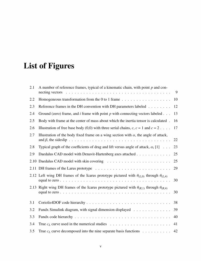
List of Figures
2.1 A number of reference frames, typical of a kinematic chain, with point p and con-necting vectors . . . . . . . . . . . . . . . . . . . . . . . . . . . . . . . . . . . . 9
2.2 Homogeneous transformation from the 0 to 1 frame . . . . . . . . . . . . . . . . . 10
2.3 Reference frames in the DH convention with DH parameters labeled . . . . . . . . 12
2.4 Ground (zero) frame, and i frame with point p with connecting vectors labeled . . . 13
2.5 Body with frame at the center of mass about which the inertia tensor is calculated . 16
2.6 Illustration of free base body (0,0) with three serial chains, c, c = 1 and c = 2 . . . . 17
2.7 Illustration of the body fixed frame on a wing section with α, the angle of attack,and β, the sideslip . . . . . . . . . . . . . . . . . . . . . . . . . . . . . . . . . . . 22
2.8 Typical graph of the coefficients of drag and lift versus angle of attack, αi [1] . . . 23
2.9 Daedalus CAD model with Denavit-Hartenberg axes attached . . . . . . . . . . . . 25
2.10 Daedalus CAD model with skin covering . . . . . . . . . . . . . . . . . . . . . . 25
2.11 DH frames of the Larus prototype . . . . . . . . . . . . . . . . . . . . . . . . . . 29
2.12 Left wing DH frames of the Icarus prototype pictured with θ(L,0) through θ(L,4)equal to zero . . . . . . . . . . . . . . . . . . . . . . . . . . . . . . . . . . . . . . 30
2.13 Right wing DH frames of the Icarus prototype pictured with θ(R,1) through θ(R,4)equal to zero . . . . . . . . . . . . . . . . . . . . . . . . . . . . . . . . . . . . . . 30
3.1 Coriolis4DOF code hierarchy . . . . . . . . . . . . . . . . . . . . . . . . . . . . . 38
3.2 Fundx Simulink diagram, with signal dimension displayed . . . . . . . . . . . . . 39
3.3 Fundx code hierarchy . . . . . . . . . . . . . . . . . . . . . . . . . . . . . . . . . 40
3.4 True cL curve used in the numerical studies . . . . . . . . . . . . . . . . . . . . . 41
3.5 True cL curve decomposed into the nine separate basis functions . . . . . . . . . . 42
v

3.6 Path of the linkages through its desired joint trajectories during the downstroke(left), and upstroke (right) . . . . . . . . . . . . . . . . . . . . . . . . . . . . . . . 43
3.7 Errors in joint positions with lift acting on body 2 . . . . . . . . . . . . . . . . . . 44
3.8 Errors in joint velocities . . . . . . . . . . . . . . . . . . . . . . . . . . . . . . . . 45
3.9 Lift on body 2 and estimated lift on body 2 . . . . . . . . . . . . . . . . . . . . . 46
3.10 Parameter error on body 2 lift . . . . . . . . . . . . . . . . . . . . . . . . . . . . . 47
3.11 Angle of attack of body 2 . . . . . . . . . . . . . . . . . . . . . . . . . . . . . . . 48
3.12 True cD curve using nine unknown functions . . . . . . . . . . . . . . . . . . . . . 48
3.13 Errors in joint positions with drag and lift acting on bodies 2−4 . . . . . . . . . . 49
3.14 Errors in joint velocities with drag and lift acting on bodies 2−4 . . . . . . . . . . 49
3.15 Parameter errors on bodies 1−4 . . . . . . . . . . . . . . . . . . . . . . . . . . . 50
3.16 Angle of attack for wing sections 1−4 . . . . . . . . . . . . . . . . . . . . . . . . 50
3.17 Errors in joint positions with drag and lift acting on bodies 2−4 . . . . . . . . . . 52
3.18 Errors in joint velocities with drag and lift acting on bodies 2−4 . . . . . . . . . . 53
3.19 Dissipative controller effort on bodies 2−4 . . . . . . . . . . . . . . . . . . . . . 53
3.20 Parameter error on bodies 1−4 in the dissipative controller simulation . . . . . . . 54
3.21 Error of the third lift parameter of body 2 . . . . . . . . . . . . . . . . . . . . . . 54
3.22 Error in the fourth lift parameter of body 2 . . . . . . . . . . . . . . . . . . . . . . 55
3.23 Angle of attack response for all bodies in the dissipative controller simulation . . . 55
3.24 Total lift acting on the Daedalus wing model in the dissipative controller simulation 56
3.25 Errors in Larus joint positions with drag and lift acting on bodies 2−4 . . . . . . . 56
3.26 Errors in Larus joint velocities with drag and lift acting on bodies 2−4 . . . . . . . 57
3.27 Dissipative controller effort on bodies 2−4 using the Larus dynamic model . . . . 57
vi

List of Tables
2.1 Notation for the discussion of moving base body models . . . . . . . . . . . . . . 18
2.2 Daedalus DH parameters . . . . . . . . . . . . . . . . . . . . . . . . . . . . . . . 26
2.3 Daedalus sample DH parameters . . . . . . . . . . . . . . . . . . . . . . . . . . . 26
2.4 Daedalus sample mass parameters . . . . . . . . . . . . . . . . . . . . . . . . . . 26
2.5 Daedalus moment of inertia parameters, kg ·m2×10−5 . . . . . . . . . . . . . . . 27
2.6 Daedalus sample relative center of mass positions . . . . . . . . . . . . . . . . . . 27
2.7 DH Parameters for the Larus model . . . . . . . . . . . . . . . . . . . . . . . . . 27
2.8 Larus sample DH parameters . . . . . . . . . . . . . . . . . . . . . . . . . . . . . 28
2.9 Larus sample mass parameters . . . . . . . . . . . . . . . . . . . . . . . . . . . . 28
2.10 Larus moment of inertia parameters, kg ·m2×10−5 . . . . . . . . . . . . . . . . . 28
2.11 Larus sample relative center of mass positions . . . . . . . . . . . . . . . . . . . . 28
2.12 Icarus right wing DH parameters . . . . . . . . . . . . . . . . . . . . . . . . . . . 29
2.13 Icarus left wing DH parameters . . . . . . . . . . . . . . . . . . . . . . . . . . . . 30
3.1 Fundx input and output for dissipative controller simulation . . . . . . . . . . . . . 39
3.2 Daedalus DH parameters used in dynamic inversion simulation . . . . . . . . . . . 40
3.3 Daedalus relative aerodynamic centers, riai
. . . . . . . . . . . . . . . . . . . . . . 41
vii

Chapter 1
Introduction and Motivation
A wide range of problems are encountered in the analysis, design and fabrication of robots thatemulate bird flight. In analysing these types of systems, the unsteady, nonlinear aerodynamicspresent significant difficulties. The low Reynolds numbers experienced by small scale aircraft alsoaffect the design of wings that improve propulsion. In addition to the importance in understandingthe complex unsteady aerodynamics, these systems require advanced flight control development toachieve stable flapping flight.Construction of such vehicles also remains formidable. Vehicles based on bird flight must bestructurally sound. Designs must account not only for the aerodynamic forces, but also for thedynamic loads induced in the flapping wings. The mechanical construction must rely on strongbut lightweight structures and materials to give the vehicle a lift/weight ratio over one. Successfulprototypes therefore require specialized fabrication and manufacturing techniques to create partsfrom materials such as carbon fiber. Electrical components, such as micro-controllers, batteries,signal processors, or sensors must be sufficiently light and compact to be a payload for a smallscale flying vehicle. Further development of light, efficient motors and electromechanical powersources is even more crucial for success of flapping wing robots. Since the mass of the motors isoften a significant proportion of weight, any increased motor mass will require stronger structuresand improved lift. For this reason, light and compact power sources remain a limiting factor in theefficiency of an electromechanical system.This thesis studies the kinematic and dynamic problems that arise in the study of articulated, flap-ping wing aircraft and the application of various control techniques to these problems. The articu-lated wing is modeled as a robotic arm, and the kinematics are analyzed using common techniquesused in the study of serial chain robots. This study also develops a method for treating the kinemat-ics and dynamics of a moving base body, or free flying system. The dynamic models are combinedwith a quasi-steady state aerodynamic model to generate the full system equations of motion. Theequations of motion are considered in the development of two nonlinear controllers which utilizeadaptation to account for uncertainties in the aerodynamic loads. The controllers are based ondynamic inversion and dissipative control techniques found in standard robotics texts, but havebeen modified to remain effective under the unique system equations. Lyapunov analysis is used
1

2
to study the stability of these nonlinear systems and is integral for the generation of update laws.The update laws allow for adaptation in the system model and as a result, increase stability andperformance.Numerical studies are carried out for the closed loop system to verify the control designs. DenavitHartenberg kinematic models are derived for various flapping wing vehicle designs developed bysenior design teams at Virginia Polytechnic Institute and State University (Virginia Tech). The sys-tem parameters, such as masses and link lengths, are chosen to represent the physical parametersof these prototypes. The desired wing trajectories are composed of joint angle functions, whichare designed for motions which the prototypes can achieve kinematically. These motions includetwo flapping modes observed in birds [2, 3], flapping and lead/lag. The amplitude and frequencyvary in bird flight depending on the level of thrust and lift required. For purposes of verifying thecontrol design, the amplitudes and frequencies were held constant. Values for the simulations werechosen considering several sources of data for level flying birds in the correct scale [2–4].
1.1 Literature Review
With the growing demand for unmanned air vehicles (UAVs), research that studies micro air ve-hicles (MAVs) has also experienced increased attention from researchers. One current trend inthese research endeavours is a focus on bio-inspired design. Researchers look for inspiration bystudying creatures such as birds [2, 3, 5–7], insects [8–11], bats [12], and even some less commonanimals such as those found in Chrysopelea, the genus of flying snakes [13–15]. Bungent and Se-elecke [12] rely on principles of bioinspired design to define three major categories of MAVs. Thefirst type includes traditional fixed wing aircraft. These are generally scaled down versions of com-mon aircraft with propeller driven propulsion systems. The issue that drives research for this classis that characteristic length greatly decreases as these vehicles are scaled down, and this inevitablyimplies they operate in a low Reynolds number regime. As Bungent and Seelecke describe, thislower Reynolds number increases viscous effects and has motivated research in other MAV flightmethods. Rotary wing MAVs constitute their second category of MAVs. These vehicles make upa significant share of the field with quadrotor vehicles being a prominent example. Lastly, flappingwing vehicles make up the third category. There has been a large increase in their number in thepast decade. Flapping wings can execute motions that some claim [6, 10, 16] are more well suitedfor low Reynolds number flight. Bungent and Seelecke detail their success using shape memoryalloy (SMA) wires in an experiment to actuate wings to match the range of motion seen in bats.Their prototype has two degrees of freedom and uses resistance as feedback in the control of theSMA actuators.Flying insects are often studied as subjects of inspiration for flapping wing flight. Singh andChopra [11] point out some benefits to flapping wing aircraft such as advanced maneuverabilityand low noise production. They investigate some aspects of hovering flight including thrust versusbeat frequency, and unsteady aerodynamics. They discuss the fact that quasi-steady aerodynamicsdo not agree with phenomenon seen in insect flight, and propose that flying insects take advantage

3
of unsteady aerodynamics in order to achieve the performance necessary for hovering flight. Theydevelop a flapping mechanism for experimental studies. It consists of two degrees of freedom ineach wing. For their scale, for vehicles that have a 148mm wing length, they find an optimal beatfrequency between 10-11 Hz. There is decreased thrust when frequency was increased beyond thispoint. They study several wing shapes, and wings are constructed using an aluminum frame withMylar film. They note that RC Microlite material is lighter but provides less lift than Mylar. Inclosing they compare the elastic and rigid wing analysis with the results obtained from the flappingapparatus.Deng et al. have published several articles that study system modeling and control design of insect-based flapping wing vehicles. The authors classify their project as research in “micromechanicalflying insects (MFIs)”. Deng et al. [9] synthesize results in their work from multiple areas of studyincluding insect biology, including sensory feedback, wing aerodynamics, body dynamics, actu-ator dynamics, sensors, and flight control. The authors note one advantage flapping wing insectshave over rotary aircraft is that they are less susceptible to environmental disturbances. The au-thors use standard quasi-steady aerodynamics to model lift and drag, and blade element theory isused for rotating wings. Blade element theory was developed by the rotary wing industry and isperformed by dividing the wing length into infinitesimal divisions and integrating along the lengthof the wing. The authors compare this aerodynamic analysis with the experimental results foundwith their prototype ‘robofly’. They discuss reference frames, kinematics and dynamics of thebase body, and compare the use of Euler angles and quaternions. The authors relate the use of the‘ocelli’ in flying insects to horizon detectors in aircraft. These use light intensity measurementsfrom the sun at multiple locations to provide support in attitude stabilization. They propose twomore methods for feedback, a magnetic compass for heading information and structures analogousto the ‘halteres’ on these insects to measure body rotations.In the second article of the series by Deng et al. [8], a high frequency periodic control problem isformulated for the underactuated system. The controller is designed for implementation with lim-ited on-board computational resources. In their control design, the authors use an LQR method forweighing performance and control effort. The authors observe that the use of high-frequency pe-riodic control with geometric control theory would be prohibitively computationally expensive foron-board implementation. The authors instead apply averaging theory to the problem which moreclosely matches standard controller design employed in helicopter flight control. Their approachdoes not guarantee asymptotic stability, but holds that the error is bounded and deemed negligiblein size from a practical sense.Taylor and Thomas in [17] look at various aspects of flapping flight stability. They first reviewtwo main approaches to achieve stability, inherent stability and active control. Inherent stability isachieved when disturbances are passively damped out. In the case of helicopter stability, increasein velocity creates a moment when the retreating blade has decreased lift and the advancing bladehas increased lift. Taylor and Thomas describe this as mildly unstable longitudinal dynamics. Sim-ilarly, flapping wings exhibit a longitudinal instability when increased velocity flow over the wingscauses bending about the chord. On the other hand, birds whose wings have sufficient stiffnessmay not be greatly affected by this behavior. The article then analyzes the flapping wing problemusing blade element theory and quasi-steady aerodynamics. Using this analysis, a flapping flight

4
vehicle model is derived that has first order stability in hover. During forward flight, stability isdependent on three terms: the coordinates of the aerodynamic center, forward inclination of theflight force vector, and sign of the pitching moment coefficient about the aerodynamic center.Leonard [18] studies the dynamics and stability of hover capable MAVs modeled after flying in-sects. Trim solutions are examined in hover, climb, and forward flight cases. A set of quasi-coordinates are used in conjunction with Lagrange’s equations to derive the state space equationsof motion for a three frame wing model. Leonard then discusses an aerodynamic model that isbased on quasi-steady potential flow. Reversed flow theory serves as a foundation for this modelwhich allows for control by adjusting the point of flow reversal across the wing. The reversedflow occurs when the leading edge becomes the trailing edge and vice versa. With precise controlof the wing rotation, a switch in flow direction before the end of one half stroke will result in anupward force while a late switch in flow direction results causes a downward force. Two airloadmodels are validated and agree very closely with each other in predicting thrust and lift in the bodyframe. Lastly, Leonard explores open loop dynamic stability using a Stroke-Averaged system andperforms the analysis using a periodic trim solution technique based on Floquent analysis. Thesimulations show that the system is naturally unstable and that wing hinge location and potentiallytrim do not seem to affect the stability. The author assumes all the bodies are rigid, and assumes aconstant inflow and viscosity model.Ansari et al. in [10] study insect flight from an aerodynamics point of view. As motivation for theirwork, they claim that insect based bioinspired flight leads to improved efficiency and manoeuvra-bility in comparison to its fixed and rotary wing counterparts. Ansari et al. [10] expand upon thebasic aerodynamic models such as in Deng et al. [8] that are based on quasi-steady formulations.The authors claim their aerodynamic models are some of the ‘most satisfactory to date’(2006)while they review a variety of approaches such as steady-state, quasi-steady, semi-empirical, andfully unsteady methods. The large lift force not accounted for in the typical quasi-steady statemodel is due to the influence of the leading edge vortices (LEV).Another study on flapping flight aerodynamics appears in [7]. The authors von Ellenrieder et al.develop a general study of flapping wing aerodynamics as applied to both insects and birds as wellas some discussion of fish and marine animals. This study contains a 2D analysis of steady cruisingand propulsion in these ‘natural flyers’. It also states that observed wing pitching in several flyinginsects is assisted by wing inertia and aerodynamic effects. In hovering flight, these contributionsmay be used for a completely passive control of the pitch. The authors consider whether flying is alimit cycle process, where there is a coupling between internal power and passive energy dissipa-tion. They suggest that a limit cycle may occur in flapping flight but conclude that further testingis necessary before it is confirmed.Gopalakrishnan et al. [19] study the formation and effects of the leading edge vortex on lowReynolds number flight (for Re= 10,000). They use an single rigid insect type wing for theirsimulations. They use a delayed-stall, unsteady aerodynamic formulation with varying angle ofattack and show that a moderate angle of attack will result in high propulsive efficiency.Mazaheri and Ebrahimi in [20] perform an aerodynamic study based on an experiment featuringflexible membrane flapping. They follow up on prior research [21] showing that an increase inthrust and lift results when the torsional stiffness in a flapping wing is decreased. The authors

5
design and test a flapping wing prototype constructed with a flexible membrane wing. They inves-tigate the relationship of thrust and lift as a function of flapping frequency, angle of incidence, andflow velocity. The mechanism is designed to oscillate between +30 and −19. For higher flappingrates, from 3Hz to 10Hz in their case, the thrust always increases. For lower flapping rates, liftforce is nearly independent of the frequency. For lower angles of incidence, a large increase in liftis observed for frequencies over 5 Hz. At high velocities, flapping rate has a small effect on lift.Angle of incidence is proportional to lift. They also noted that angle of incidence and thrust areinversely proportional.Aditya and Malolan in [5] investigate the effect of the Strouhal number on the propulsion of aflapping wing. In this article, the Strouhal number is calculated as:
S t =f A
U∞=
2 · f ·bsemi−e f f · sin(φ2
)U∞
where A is amplitude, the semi-span of the wing is bsemi−e f f , the flapping angle is φ, the flowvelocity or forward speed is U∞, and flapping frequency is f . The authors recommend a range ofvalues for the Strouhal number in wing design. They observe that a range of 0.2 to 0.4 is typical forbirds. Fast flying birds exhibit Strouhal numbers near S t = 0.2 and slower flying birds have valuesaround S t = 0.4. They test a 15cm span flapping mechanism and find their highest peak propulsiveforces result from a Strouhal number between 0.1−0.2.Taylor et al. [22] agrees that Strouhal number is also crucial for efficiency in flapping flight. Thesame range of Strouhal number S t = 0.2 to 0.4 is observed for both flying animals and marineanimals such as fish, dolphins and sharks. The investigators perform a statistical analysis and findintermittent flying birds to have a mean Strouhal number S t = 0.34 and for direct flyers to have aStrouhal number S t = 0.20. In summary Taylor et al. in [22] create a rule of thumb that the velocitywill be three times the product of the flapping frequency and amplitude.Han [3] investigates unsteady aerodynamics in stable flight of a seagull. He notes that combin-ing three “flapping, folding, and lead/lag” modes generates an optimal lift scenario. He uses aboundary element method to perform the unsteady aerodynamic analysis. The kinematic modelused in this study selects the three DOF system introduced by Liu et al. [2]. This choice includesa flapping angle ψ1, a folding angle ψ2 and lead/lag angle φ2. Using only one of these flappingmodes decreases drag for flapping, folding, and lead/lag. Using a flapping mode alone increaseslift coefficient the rest of the wing fixed. Of the combined tests, flapping and folding generatesthe greatest thrust generation of all the tests, and flapping with lead/lag produced the second bestlift coefficient. The overall highest lift coefficient is achieved via the combination of the three,although thrust coefficient is slightly decreased from the flapping and folding combination (0.2 to0.1704).Other than the data contained in engineering articles, there are few biological studies on birdswhich include quantitative research. Tobalske at the University of Montana Flight Laboratory per-forms many quantitative empirical studies on skeletal mechanics, aerodynamics and mechanicalpower of birds. Many of the experiments provide useful tests on live birds, which document pre-cise kinematic and aerodynamic data of bird flight. In a study of tip-reversal by Crandell andTobalske [23], an experiment is performed using four synchronized high-speed cameras to obtain

6
in vivo angle of attack and coefficient of lift for an rock dove during upstroke and downstroke.The downstroke produced an estimate of 115% of the bodyweight, at an effective wing length of0.314m.Liu [2] also performs quantitative in vivo tests on birds and geometric study of wings from birdspecimens. Liu uses footage of level-flying, or steady flying seagulls, cranes and geese. He devel-ops a wing model with three degrees of freedom that is able to represent the motion of the threebirds. The seagull wing used in this investigation can be approximated from illustrations and isnear to 0.6m. The investigation also documents wing geometry of several birds including the Seag-ull, Merganser, Teal and Owl. Specifically, the author studies airfoil parameters such as thickness,camber, and chord length.Some in vivo flight testing appears as early as 1982 in the Ph.D thesis by Scoley [4]. Althoughthe video photography and processing is primitive compared to today’s standard, some morpho-logical data is still relevant and can be used as a reference for relative scaling. Articles such asthese contain extensive collections of data for different species. Two species of the genus Larusare examined, the Black Headed Gull (Larus Ridibundus), and Common Gull (Larus Canus). TheCommon Gull has average mass of 0.388kg, average wingspan of 1.13m and an average strokefrequency of 3.76 Hz. The smaller Black Headed Gull has an average mass of 0.251kg, averagewingspan of 0.94m and average stroke frequency of 3.84 Hz. The flighted bird with the largestwingspan in this study is the Wandering Albatross, Diomedea Exulans. It has a mass of 8.5kg,wingspan of 3.42m, and flapping frequency of 2.61 Hz.In summary, although there have been numerous studies that model flapping flight, only a feweffort that study the control of flapping wing have appeared in the literature. This thesis constructsdynamic models of articulated flapping wing robots and synthesizes controllers that guaranteetracking of flapping motions. Chapter 2 begins with a derivation of the equations of motion forsome classes of flapping wing robotic systems. Chapter 3 discusses the adaptive controller derivedin this thesis. The thesis concludes in Chapter 4, where a summary of accomplishments is givenand future work is outlined.
7
1.2 Nomenclature List
αi Angle of attack for ith wing sectionβi Side slip for ith wing sectionγ Learning gainρ Density of surrounding fluidσ Error tracking term for dissipative controllerτ Control input vectorΦ Vector of basis functionsω Angular velocityΩ Vector of unknown parametersΩ Vector of unknown parameter estimatesAw,i 2D wing area of body ib1, b2, b3 Body fixed frame unit vectorsB Control influence matrixcD Drag coefficientcL Lift coefficientC Nonlinear Coriolis matrixDi Drag force on ith wing sectionG Control Gain MatrixH j
i DH transformation matrix from frame i to frame jI Inertia tensorJv Velocity Jacobian matrixJω Angular velocity Jacobian matrixLi Lift force on ith wing sectionM Generalized inertial matrixn Vector of nonlinear Coriolis and centripetal acceleration termsna Vector of unknown aerodynamic loadsq Vector of generalized coordinatesQi Generalized force vectorδr Virtual displacement vectors1, s2, s3 Stability axis unit vectorsu,v,w Velocity components for ith wing sec.v The velocity of aerodynamic center w.r.t. fluidV Lyapunov candidateδW Virtual workX System states

Chapter 2
Dynamic Models of Flapping Wing Robots
2.1 Review of Robot Kinematics
Kinematics of a robotic systems is complex since a typical system is composed of numerous rigidbodies. Descriptions of such systems often introduce several coordinate frames, or frames of refer-ence, to define kinematic variables. In this thesis, a frame is defined by a right hand, orthonormalset of unit vectors. Figure (2.1) illustrates a typical collection of frames. We will write
x0 y0 z0
as the basis for the 0 frame, and
x1 y1 z1
as the basis for the 1 frame and so forth. An arbitrary
vector a can be expressed in terms of its components or coordinates relative to any other bases de-fined in the problem. In this thesis we choose to represent the coordinates of the vector a relativeto frame i as ai.
ai =
ai
1ai
2ai
3
a = ai1xi + ai
2yi + ai3zi
We define rip to be the coordinates relative to the frame i of the position vector that connects the
origin of frame i to point p. Likewise, the vector connecting two frames will be denoted as ri, j forthe vector from the origin of frame i to the origin of frame j. Any frame position relative to theground frame will appear as ri B r0,i.
2.1.1 Rotation Matrices
In the study of robot kinematics, orientation between two different, right handed, orthogonal framesis represented by rotation matrices. The 3× 3 rotation matrix that relates the frames 0 and 1 is
8

9
𝒓𝑝1
𝒓0,1
𝒛1
𝒚1 𝒙1
𝒙0 𝒚0
𝒛0
𝑝
𝒓𝑝2
𝒓1,2
𝒛2
𝒚2 𝒙2
𝒛𝑛
𝒚𝑛 𝒙𝑛
𝒓𝑝0
𝒓𝑝𝑛
𝒓2,𝑛
Figure 2.1: A number of reference frames, typical of a kinematic chain, with point p and connect-ing vectors
written as R10 and is defined as:
R10 =
x0 ·x1 y0 ·x1 z0 ·x1x0 ·y1 y0 ·y1 z0 ·y1x0 · z1 y0 · z1 z0 · z1
where x0,y0,z0 and x1,y1,z1 denote the right handed orthogonal bases of the 0 and 1 frame, re-spectively. The defining property of a rotation matrix is that its inverse is equal to its transpose,and therefore we can write (
R10
)−1=
(R1
0
)T
From this definition, it is clear that (R1
0
)T= R0
1
The rotation matrix R10 maps the components of a vector relative to the 0 frame into components
relative to the 1 frame.r1 = R1
0r0
2.1.2 Homogeneous Transforms
While relative rotation is represented in terms of rotation matrices, rigid body motion is specifiedin terms of homogeneous transformations. A homogeneous transformation describes both rotation

10
and displacement between reference frames. This topic is covered in many standard sources onrobot kinematics [24–26]. The relative translation r1
0,1 contains the coordinates relative to the 1frame the vector that defines the position of the 1 frame relative to the 0 frame. The homogeneoustransform that describes the rigid body motion between the 0 and 1 frames is written as H1
0, definedbelow.
H10 =
[R1
0 r11,0
0 1
]The homogeneous transform can then be used to relate the homogeneous coordinates of any point
𝒓𝑝1
𝒓1,0
𝒛1
𝒚1 𝒙1
𝒙0 𝒚0
𝒛0
𝑝 𝒓𝑝0
Figure 2.2: Homogeneous transformation from the 0 to 1 frame
in reference frame 0 to reference frame 1. The homogeneous coordinates in frame 0 are denotedas r0 and the homogeneous coordinates for frame 1 are r
1.[r1
p1
]= H1
0
[r0
p1
]r
1p = H1
0r0p
Both the homogeneous transform and rotation matrix can be combined to describe the kinematicsof a chain. For example, the homogeneous transform between the third and the ground referenceframe, in terms of the homogeneous coordinates, is obtained as
r3 = H3
2H21H1
0r0 = H3
0r0

11
2.1.3 Denavit-Hartenberg Convention
One of the most popular techniques used to represent robot kinematics is the Denavit-Hartenberg(DH) Convention. Typically, six parameters, three translations and three rotations, are necessaryto define the relative location and pose of two reference frames. By imposing some constraintson how the adjacent frames are defined, the DH convention introduces a set of four parametersto define relative pose and orientation, two angles and two scalar translation values. The mainassumption in the DH Convention is that, for adjacent frames i and i− 1 in a serial chain, the xiaxis is perpendicular to and intersects the zi−1 axis. The DH parameters then orient the i−1 framerelative to the i frame in terms of the following four parameters:
1. The displacement di translates the i frame in the direction of zi−1.
2. The offset ai translates the i frame along the xi−1 axis.
3. The rotation θi rotates the i frame about zi−1.
4. The twist αi lastly rotates the i frame about its xi axis.
The parameters introduced above are discussed further in [25], and are illustrated in Figure (2.3).Using this standard notation, a rotation matrix and homogeneous transform that define the rigidbody motion can be derived for any two successive frames in a kinematic chain. The rotationmatrix contained in the DH transformation can be expressed in terms of the two rotation matricesthat are defined via an intermediate frame B [25]:
Rii−1 = Ri
BRBi−1
Rii−1 =
cosθi sinθi 0−sinθi cosθi 0
0 0 1
·1 0 00 cosαi sinαi0 −sinαi cosαi
Ri
i−1 =
cosθi sinθi 0−cosαi sinθi cosαi cosθi sinαisinαi sinθi −sinαi cosθi cosαi
The homogeneous transform can be constructed from the DH parameters using the rotation matri-ces above and the two translational parameters ai and di. The translation ri
i−1 can be constructedby inspection from Figure (2.3) and is a function of θi, di, and ai.
Hii−1 =
[Ri
i−1 rii−1,i
0 1
]ri
i−1,i =
ai cosθiai sinθi
di
Hi
i−1 =
cosθi sinθi 0 ai cosθi
−cosαi sinθi cosαi cosθi sinαi ai sinθisinαi sinθi −sinαi cosθi cosαi di
0 0 0 1

12
𝜃𝑖
𝒛𝑖
𝒚𝑖
𝒙𝑖
𝒙𝑖−1
𝒚𝑖−1
𝒛𝑖−1
𝛼𝑖
𝑑𝑖
𝑎𝑖
Figure 2.3: Reference frames in the DH convention with DH parameters labeled
2.1.4 Angular Velocity and Translational Velocity
Many robotic systems are constructed from chains of rigid bodies. Standard methods have beendeveloped to derive the velocities or angular velocities in a kinematic chain. We consider a casewhere the point p is fixed in the ith frame and is denoted by ri
p. The mapping between the frame iframe and frame i−1 is determined by the homogeneous transformation matrix Hi−1
i . The positionvector ri−1
p can be decomposed asri−1
p = Ri−1i ri
p + ri−1i−1,i
This formula is differentiated with respect to time to find the velocity.
vip =
ddt
rip
The frame number is omitted in both the velocity and position for the zero frame:
vp B v0p rp B r0
p
For a DH kinematic chain, the velocity of a point p in the ground frame is found using the velocityof frame i in the ground frame, and a rotation rate about its zi axis, θi. The frames and point p areillustrated Figure (2.4)
vp = θizi× rip + vi (2.1)

13
If the frame velocity, vi, is calculated with Equation (2.1), recursion can be used to find velocities
𝒓𝑝𝑖
𝜃𝑖
𝒓𝑖
𝒛𝑖
𝒚𝑖 𝒙𝑖
𝒙0 𝒚0
𝒛0
𝑝
Figure 2.4: Ground (zero) frame, and i frame with point p with connecting vectors labeled
for an entire series of frames. This idea is fundamental in joint-space kinematics for robotic link-ages that form kinematic chains.The velocity Jacobian Jvi is defined to yield the components of velocity relative to the ith frame.We suppress the frame number when the Jacobian yields components relative to the basis for theframe 0 so that Jv B Jv0 . The components of the velocity of point p relative to the ground frame isthen
vp = Jvq (2.2)
where the vector q = q1 · · · qNT is an N vector of derivatives of the joint variables. The angular
velocity Jacobian Jω is similarly defined as
ωp = Jωq (2.3)
By using Theorem 2.15 in Kurdila, et al. [25], finding the angular velocity Jacobian is a trivialprocess. When joint variables are selected to be either relative rotations or displacements, angularvelocity vectors can be summed by adding the angular velocities of adjacent frames. Specifically,the angular velocity Jacobian can be generated using
Jω =[ρ1z0
0 ρ2R01z1
1 · · · ρNR0N−1zN−1
N−1
]In this equation, ρi is 1 for a revolute joint and 0 for a prismatic joint [24–26]. Similarly, assumingthat each joint is revolute, the velocity Jacobian is found to be
Jv =[z0
0× (r01− r0
0) R01z1
1× (r02− r0
1) · · · R0N−1zN−1
N−1× (r0N − r0
N)]

14
The position vectors r1 · · · rN represent the position vectors from the zero frame to the ith frame.For prismatic joints, we have instead
Jv =[z0
0 z01 · · · z0
n
]
2.2 Lagrange’s Equations
Once a kinematic description of the robotic system has been constructed, it remains to derive theequations governing the motion of the robot. Numerous approaches to this problem have been de-veloped in the literature. These methods can be based on techniques of analytical mechanics, suchas Lagrange’s equations, on Newton-Euler formulations, or other principles such as Kane’s equa-tions. All techniques have relative advantages and disadvantages. As an extension of Hamilton’sPrinciple, Lagrange’s equations of motion serve as a convenient and popular way of generating theequation of motion for mechanical systems. In general, these equations can be written
ddt
(∂T∂q
)−∂T∂q
+∂V∂q
= Q
In the above expression, the potential energy of the system is V , T is the kinetic energy, q is thevector of generalized coordinates, and Q is the vector of generalized forces. The generalized forcesarise from the formulation of the virtual work done by external nonconservative forces acting onthe system. If external force Fp acts at the physical point p, the virtual work is defined as thesum [25]
δWnc =∑
pFp ·δrp
Virtual work of the nonconservative external forces is then calculated in terms of the generalizedforces.
δWnc =∑i=1
Qi ·δqi = QTδq = δqTQ
It is often assumed that kinetic energy is a quadratic function of the generalized coordinates. Thekinetic energy then has the form
T =12
qTM(q)q (2.4)
Such systems are known as T2 or natural systems [27]. It is also commonly assumed that potentialenergy is a function of only the generalized coordinates, that is,
V = V(q)
If both of these conditions hold true, the equations of motion for the system can be written in ageneral form
M(q(t))q(t) = n(q(t), q(t), t) + B(q(t))τ(t) (2.5)

15
The vector n is a collection of nonlinear terms due to centripetal or Coriolis effects and is a functionof the generalized coordinates and their derivatives. The vector τ is the vector of control inputs.In this thesis all of the joints are assumed to be driven by a rotational actuator. Because all of thejoints contain a rotary actuator, the control influence matrix is the B identity matrix [25]. When theactuation scheme changes, B is determined via calculation of virtual work. This will be discussedin more detail in Section (2.3).
2.2.1 Fixed Base Body
Two classes of robotic systems are studied in this thesis, those that have a base body fixed in theinertial frame, and those that do not. We first discuss the case where the base body is fixed inthe inertial frame since the presentation is simpler. This discussion motivates the approach for thecase where the base body is in motion. Robotic systems that have a base body fixed in the inertialframe are appropriate for robots fixed in laboratory or wind tunnel experiments. We assume thatthe robot is fully actuated. The kinematics for this case can be cast via standard approaches forrobotics. The set of equations of motion for the flapping wing robot will have the form of Equation(2.5). However, it is important to note that in the study of flapping wing robots not all the terms thatappear in the robot equations of motion are measurable or known. The aerodynamic contributionsto the virtual work are not usually available. The equations of motion include a second nonlinearterm na that represent the aerodynamic effects on the system.
M(q(t))q(t) = n(q(t), q(t), t) + na(q(t), q(t), t) + B(q(t))τ(t) (2.6)
The functional form of the aerodynamic contributions is studied in Section (2.3). As in manyrobotics formulations, the mass matrix is generated in our model through the use of Jacobian ma-trices. This method provides explicit expansions of the translational and rotational kinetic energy.First we recall the standard Lagrangian formulation for kinetic energy of a single body i using thevelocity at the center of mass vi, angular velocity ωi, and inertia tensor about the center of mass Ii.The frame used for calculating the inertia tensor is depicted in Figure (2.5).
Ti =12
mivTi vi +
12ωT
i Iiωi (2.7)
From Section (2.1.4), we recall the Jacobian definitions in Equation (2.2) and Equation (2.3).
vp = Jvq ωp = Jωq
The velocity is calculated at the center of mass for each link, denoted as point g(i) for the center ofmass for link i. The velocity Jacobian used in calculation of vi is introduced as Jv
g(i). The angularvelocity Jacobian introduced for calculating ωi, the angular velocity of link i, is designated as Jωi .The velocity equations are substituted into Equation (2.7), then the generalized coordinate vectorsare factored.
Ti =12
mi(Jv
g(i)q)T (
Jvg(i)q
)+
12
(Jωi q
)TIi(Jωi q
)

16
𝑥𝑖
𝑦𝑖
𝑧𝑖
𝑥1′
𝑦1′
𝑧1′
𝑐𝑚
Figure 2.5: Body with frame at the center of mass about which the inertia tensor is calculated
Ti =12
qT(mi
(Jv
g(i)
)TJv
g(i) +(Jωi
)TIiJωi
)q
This formula is then simplified by introducing two matrices, the translational generalized inertiacomponent Mv
i , and rotational generalized inertia component Mωi . The contribution due to trans-
lational motion to the mass matrix is calculated via the identity
Mvi = mi
(Jv
g(i)
)TJv
g(i),
while the contribution due to rotational motion is
Mωi =
(Jωi
)TIiJωi
In this equation Ii is the inertia matrix relative to the same basis used in the definition of theJacobian matrix Jωi . After Mv
i and Mωi are generated, the mass matrix for body i is compiled by
summing these two matrices [25].Mi = Mv
i + Mωi
The total kinetic energy for a single body i can then be assembled in the form similar to Equation(2.4)
Ti =12
qTMi(q)q
The total energy for a fixed base robotic system is found by summing the kinetic and potentialenergies for all bodies.
2.2.2 Moving Base Body
To construct a kinematic and dynamic model for an ornithopter in flight, the fixed base constraint isnot applicable. In this thesis we assume that there is one free base body having no directly actuateddegrees of freedom, with one or more attached serial chains. We assume there are no closed loopsin the system. The kinematic chains will be modeled using the DH convention. This model is

17
illustrated in Figure (2.6). This figure shows a base body with two kinematic chains and illustratesthe numbering convention used. The base body is labeled with a body fixed reference frame (0,0),and ground frame is labeled as G. Links in the chains are labeled as (c,k), where c is the chainnumber and k is the element in chain c. A point on body k in chain 1 is labeled as p(1,k). A standardnotation is developed for the discussion of the kinematics and dynamics of a moving base bodysystem and summarized in Table (2.1).
(0,0)
G
(1,1)
(1,2) (1,k)
p(1,k)
(2,1)
(2,2)
(2,3)
chain c chain 1
chain 2
Figure 2.6: Illustration of free base body (0,0) with three serial chains, c, c = 1 and c = 2

18
Table 2.1: Notation for the discussion of moving base body modelsName Symbol DescriptionChain c Chain numberFrame, body (c,k) Chain c, link kPoint p(c,k) Point p on body c,kGeneralized coordinate q(c,k) Joint coordinate at chain c, link kVector of joint coordinates qc All coordinates in chain c
Velocity of body fixed point v(c,k)p(c,k)
Velocity of point p in body (c,k) rela-tive to frame (c,k)
Angular velocity of frame ω(c1,k1),(c2,k2)Angular velocity of link (c1,k1) relativeto (c2,k2)
Velocity Jacobian Jv0(c,k)
Jacobian at body origin (c,k) relative tobase frame (c,0)
Jvp(c,k)
Jacobian at point p on body (c,k) rela-tive to base frame (c,0)
Jv0(c,0)
Jacobian at base of chain c, relative tothe base body
Angular velocity Jacobian Jω(c,k)Jacobian at body (c,k) relative to baseframe (c,0)
Jω(0,0)Jacobian at base body relative to theground frame G.
Mass of link m(c,k) Mass of link (c,k)Rotational inertia matrix I(c,k) -Total mass matrix Msys -Link mass contribution M(c,k) Contribution for link (c,k)Translation link contribution Mv
(c,k) -Rotational link contribution Mω
(c,k) -Number of chains nc -Number of links (coordinates) inchain i
nci nc1 for chain 1 or nc3 for chain 3
Number of coordinates in chainand body
nTki Sum of nci + nc0
Total number of coordinates insystem
nT -
The first step in the analysis of the moving base body dynamics calculates the velocity for a pointp fixed in the kth link of the chain c. This is found by adding the velocity of the base of chain c andthe relative velocity of p.
vp(c,k) = vc,0 + v(c,0)p(c,k)
The relative velocity of the end of the chain can be found using the velocity Jacobian found in

19
conventional robotic kinematics [24–26]. The relative chain Jacobian in full terms is written asJvG
(c,0),p(c,k) to specify that the velocity is calculated relative to the chain base (c,0), and in theground frame basis G. The simplified form, to which it is referred to in the following text is Jv
p(c,k).We must introduce another Jacobian JvG
G,0(c,0) to find the velocity of the base of the chain relative tothe ground frame and in terms of the body coordinates q0. The ground frame G of the chain baseJacobian is suppressed in the subscript and superscript and the Jacobian appears as Jv
0,(c,0).
vp(c,k) = Jv0(c,0)q0 + Jv
p(c,k)qc =[Jv
0,(c,0) Jvp(c,k)
] [q0qc
]The angular velocity can be calculated in a similar fashion using two angular velocity Jacobianmatrices. The first Jacobian in full form is JωG
G,(0,0), indicating the frame (0,0) or free body framerotates relative to the ground frame G, and in the ground frame basis. The first angular velocityJacobian is abbreviated as Jω(0,0). The second angular velocity Jacobian rotates the body (c,k) fixedin the chain base frame (c,0), and without simplification it is denoted as JωG
(c,0),p(c,k). The simplifiedform used in the text is Jωp(c,k).
ω(c,k) = Jω(0,0)q0 + Jω(c,k)qc =[Jω0(c,0) Jωp(c,k)
] [q0qc
]The kinetic energy of a body k in a chain c is found by calculating the contributions due to trans-lation and rotation. The translational component is found using the mass and the velocities at thecenter of mass of an link.
T v(c,k) =
12
m(c,k)vTg(c,k)vg(c,k)
=12
m(c,k)[qT
0 qTc
] (Jv
0(c,0)
)T(Jv
g(c,k)
)T
[Jv0(c,0) Jv
g(c,k)
] [q0qc
]
=12
m(c,k)[qT
0 qTc
] (Jv
0(c,0)
)TJv
0(c,0)
(Jv
0(c,0)
)TJv
g(c,k)(Jv
g(c,k)
)TJv
0(c,0)
(Jv
g(c,k)
)TJv
g(c,k)
[q0qc
]The mass matrix contribution from this equation can be extracted from the terms listed below. Mv
0,0 Mv0,(c,k)(
Mv0,(c,k)
)TMv
(c,k),(c,k)
= m(c,k)
(Jv
(c,0)
)TJv
(c,0)
(Jv
(c,0)
)TJv
g(c,k)(Jv
g(c,k)
)TJv
(c,0)
(Jv
g(c,k)
)TJv
g(c,k)
The rotational kinetic energy is found using the inertia matrix I(c,k) and angular velocity Jacobians.The contribution of rotational motion to the generalized mass matrix is calculated in terms of theinertia about the center of mass of each link (c,k).
Tω(c,k) =
12ωT
(c,k)I(c,k)ω(c,k)
=12
[qT
0 qTc
] [Jω(0,0) Jω(c,k)
]TI(c,k)
[Jω(0,0) Jω(c,k)
] [q0qc
]

20
In the above expression, the Jacobian matrices and the inertia matrix must be expressed in termsof the same basis. In this case, the ground frame is implied. The mass matrix contributions fromthe rotational kinetic energy are computed below. Mω
0,0 Mω0,(c,k)(
Mω0,(c,k)
)TMω
(c,k),(c,k)
=[Jω(0,0) Jω(c,k)
]TI(c,k)
[Jω(0,0) Jω(c,k)
]To complete the mass matrix for each chain, the rotational and translational components aresummed for each link in the chain.[
M0,0 M0,c(M0,c
)T Mc,c
]=
nci∑k=1
Mv0,0 Mv
0,(c,k)(Mv
0,(c,k)
)TMv
(c,k),(c,k)
+
Mω0,0 Mω
0,(c,k)(Mω
0,(c,k)
)TMω
(c,k),(c,k)
The final step in generating the mass matrix for a system in which the base body is in motion is thecalculation of the contribution from the base body. The procedure for calculating this contributionis trivial once the chain kinetic energy formulations are completed.
T v(0,0) =
12
m(0,0)vTg(0,0)vg(0,0)
=12
m(0,0)qT0
(Jv
g(0,0)
)TJv
g(0,0)q0
Tω(0,0) =
12ωT
(0,0)I(0,0)ω(0,0)
=12
qT0
(Jωg(0,0)
)TI(0,0)Jωg(0,0)q0
The total mass matrix of the system Msys can then be compiled from the constituent mass matrices.
It will have dimensions nT ×nT where nT =nc∑
i=0nci , the sum of the number of links in each chain, for
every chain. The base body mass matrix and M0,0 values from each element are summed together.Within each chain the terms M0,c and Mc,0 will compose the first horizontal row and first verticalcolumn, respectively. The diagonal, not including the first element, will be composed of Mc,c fromeach chain. The matrix Msys will appear in the form:
Msys =
M0,0 M0,1 M0,2 · · · M0,cM1,0 M1,1 0 · · · 0M2,0 0 M2,2 · · · 0
......
... . . . ...Mc,0 0 0 · · · Mc,c
The total kinetic energy for the system then appears as:
Tsys =12
[qT
0 qT1 · · · qT
nc
]Msys
q0q1...
qnc

21
2.3 Aerodynamic Model
In this section, we discuss the calculation of the contribution of the aerodynamic loads to theequations of motion from a wing composed of a single kinematic chain. We simulate the freebase body case by introducing a velocity of the surrounding fluid. The unknown aerodynamiccontributions to the governing equations arise from the virtual work performed by the aerodynamicforces. We let rai be the position vector of the aerodynamic center of the ith wing section in theinertial frame. The total virtual work is the sum of the external aerodynamic force(s) Fai for Nbodies in a chain dotted with the virtual displacement δrai of the point of application of Fai .
δW =
N∑i=1
Fai ·δrai =
N∑i=1
Qi,a ·δqi
By convention there are two rotations, the sideslip βi and the angle of attack αi, that are used todefine the lift and drag forces on a wing. For a typical calculation on wing section i, we supposefirst that the body fixed frame Bi is defined in terms of the unit vectors b1,i, b2,i, and b3,i at theaerodynamic center of the body. The rotation matrix that maps body fixed Bi frame to the windframe S i is constructed by concatenating two single axis rotation matrices. First, an intermediateframe Ci is defined in terms of the unit vectors c1,i, c2,i, and c3,i that are obtained by rotating thebasis vectors of the Bi frame through the angle of attack αi about the c2,i = b2,i axis. Figure (2.7)depicts a wing body with body fixed axis b1, b2, and b3 with the velocity vai aligned with the windaxis. The wind frame S i is subsequently defined in terms of the unit vectors s1,i, s2,i, and s3,i thatresult when the basis vectors for the intermediate Ci frame are rotated through the sideslip βi aboutthe s3,i = c3,i axis. The product of these single axis rotations define the rotation matrix RS i
Bi(αi,βi)
which can be used to transform the coordinates of any vector in the Bi frame to the S i frame.s1,is2,is3,i
=
cosβi sinβi 0−sinβi cosβi 0
0 0 1
· cosαi 0 sinαi
0 1 0−sinαi 0 cosαi
b1,ib2,ib3,i
By definition, the lift and drag forces on any wing section constitute the aerodynamic force vectoracting on the ith wing section via the expression
Fa,i = −Di(s1,i)−Li(s3,i)
Lift and drag are approximated using a standard two-dimensional, quasi-steady aerodynamic modelin this thesis. Furthermore, the lift and drag forces are assumed to act at the aerodynamic centerand therefore the moment is ignored. We suppose ρ is the density of fluid surrounding the wing,vai is the velocity of the aerodynamic center with respect to the ground frame, vw is the velocityof the fluid with respect to the ground frame, and Aw,i is the two dimensional wing area enclosedbetween the leading edge and the trailing edge of the ith wing section. The functions cDi(αi) andcLi(αi) are the drag and lift coefficients, respectively, for wing section i as a function of the angleof attack. These are assumed unknown in this paper. See Figure 2.8 for example plots of typical

22
𝒗𝑎𝑖
𝑥 2
𝑦 2
𝑧 2
𝑏 2
𝑏 3
𝑏 1
𝛼
𝛽
Figure 2.7: Illustration of the body fixed frame on a wing section with α, the angle of attack, andβ, the sideslip
functions cLi(αi) as the angle of attack αi varies. Pictured is the lift coefficient for an S1223 airfoilat low Reynolds number Re = (2x10²) measured in wind-tunnel experiments [1]. The lift and dragon the ith section are computed as
Li =12ρ‖vw−vai‖
2cL(αi)Aw,i
Di =12ρ‖vw−vai‖
2cD(αi)Aw,i
The strategy for calculating the virtual work due to aerodynamic forces proceeds by finding the ve-locities of each aerodynamic center. These velocities are a function of the generalized coordinates.
vai = vai(q1, . . .qN)
We write the total equivalent velocity of the aerodynamic center of wing section i in the formvTi = vw − vai = uai bi,1 + vai bi,2 + wai bi,3. The angle of attack αi and sideslip βi is defined by this

23
Figure 2.8: Typical graph of the coefficients of drag and lift versus angle of attack, αi [1]
velocity and can therefore be found using the following formulae:
αi = tan−1(wai(q1, . . .qN , q1, . . . qN)uai(q1, . . .qN , q1, . . . qN)
)βi = sin−1
(vai(q1, . . .qN , q1, . . . qN)‖vTi(q1, . . .qN , q1, . . . qN)‖
)The 3×N velocity Jacobian matrix can be formed to find the vector of aerodynamic center veloci-ties.
vai = Jvai
qThis standard calculation for kinematic chains is discussed in numerous references, see [24,25,28].The rotation matrix RBi
0 maps the velocity Jacobian from the zero frame to the body fixed frame.As a consequence, the velocity is written
vBiai =
uai
vai
wai
= RBi0 JvBi
ai q = Jvai,Bi
q
The virtual displacements of the aerodynamic centers can also be found using the velocity Jacobianin either the zero frame or body fixed frame.
δrai = Jvaiδq
δrBiai = JvBi
ai δq = RBi0 Jv
aiδq
With the expressions above, we have enough information to calculate the virtual work due toaerodynamic forces. The drag and lift for each wing section can be transformed to the body fixedframe using the proper rotation matrix.
δWi = Fa,i ·δra

24
δWi = −Di,0,−LiRS iBi
JvBiai δq
It follows that the generalized forces due to aerodynamic loads on each wing section i can bewritten as
Qa =
N∑i=1
−(JvBi
ai
)T (RS i
Bi
)T
Di0Li
We introduce the matrix Ψ,
Ψ = −
[(J
vB1a1
)T (RS 1
B1
)T. . .
(J
vBNaN
)T (RS N
BN
)T]
1 00 00 1
· · ·1 00 00 1
with the right hand component of size 3×2N. The generalized forces due to the aerodynamics canbe written as
Qa =Ψ
D1L1...
DNLN
=ΨF
Control synthesis will be based on the state space form of the governing equations[X1X2
]=
]=
[X2
M−1n
]+
[0
M−1Ψ
]F +
[0
M−1B
]τ
where X1 = q and X2 = q. The final step in preparing the governing equations for control synthesisintroduces representations of the unknown drag and lift coefficients cDi(αi) and cLi(αi) for eachwing section i
DiLi
=
12ρ‖vw−vai‖
2Aw,i
∑i ΩDi,kφDi,k(αi)∑k ΩLi,kφLi,k(αi)
(2.8)
=
[ΩT
Di0
0 ΩTLi
]12ρ‖vw−vai‖
2Aw,iΦDi12ρ‖vw−vai‖
2Aw,iΦLi
=ΩT
i Φi
We assemble all the aerodynamic forces and construct
D1L1...
DnLn
=
ΦTD1
0 · · · 0 00 ΦT
L10
... . . .0 ΦT
DN0
0 0 0 ΦTLN
ΩD1
ΩL1...ΩDN
ΩLN
=ΦTΩ
25
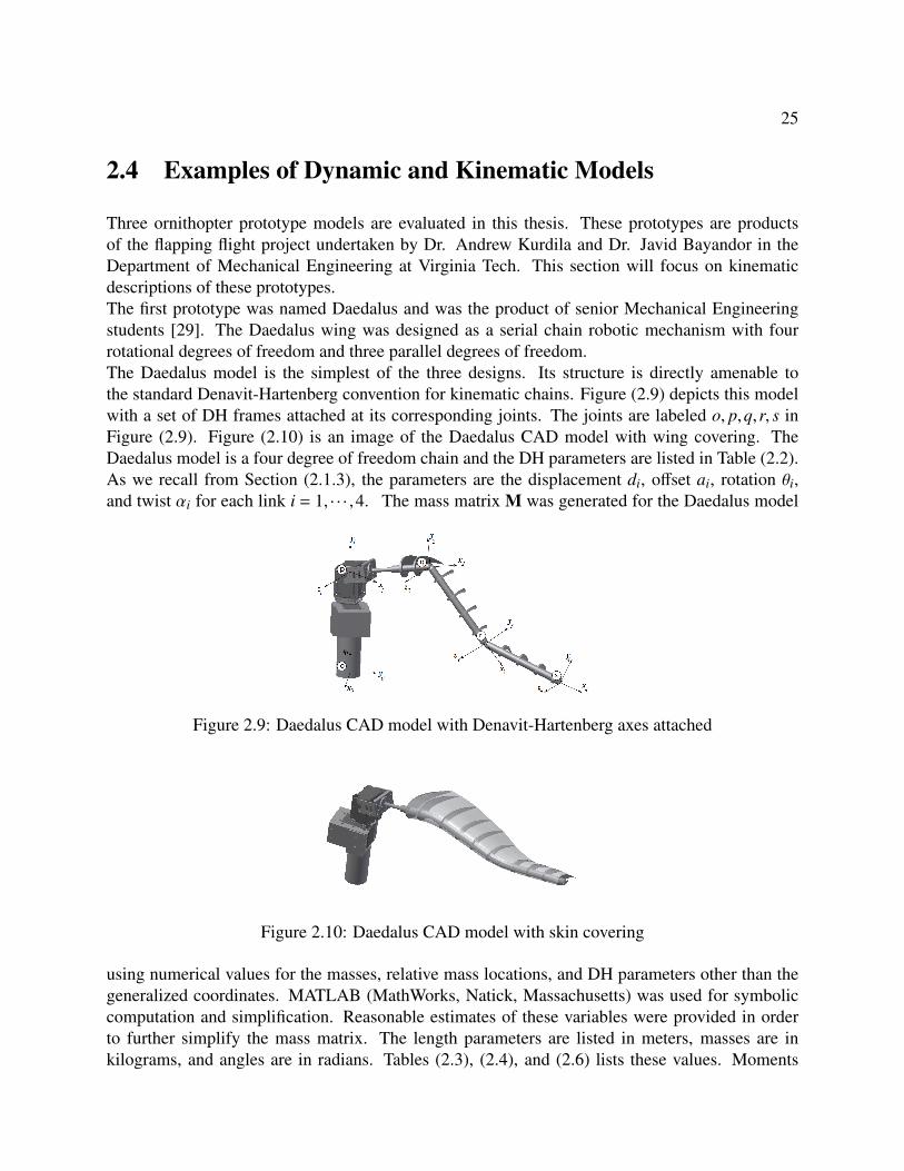
2.4 Examples of Dynamic and Kinematic Models
Three ornithopter prototype models are evaluated in this thesis. These prototypes are productsof the flapping flight project undertaken by Dr. Andrew Kurdila and Dr. Javid Bayandor in theDepartment of Mechanical Engineering at Virginia Tech. This section will focus on kinematicdescriptions of these prototypes.The first prototype was named Daedalus and was the product of senior Mechanical Engineeringstudents [29]. The Daedalus wing was designed as a serial chain robotic mechanism with fourrotational degrees of freedom and three parallel degrees of freedom.The Daedalus model is the simplest of the three designs. Its structure is directly amenable tothe standard Denavit-Hartenberg convention for kinematic chains. Figure (2.9) depicts this modelwith a set of DH frames attached at its corresponding joints. The joints are labeled o, p,q,r, s inFigure (2.9). Figure (2.10) is an image of the Daedalus CAD model with wing covering. TheDaedalus model is a four degree of freedom chain and the DH parameters are listed in Table (2.2).As we recall from Section (2.1.3), the parameters are the displacement di, offset ai, rotation θi,and twist αi for each link i = 1, · · · ,4. The mass matrix M was generated for the Daedalus model
Figure 2.9: Daedalus CAD model with Denavit-Hartenberg axes attached
Figure 2.10: Daedalus CAD model with skin covering
using numerical values for the masses, relative mass locations, and DH parameters other than thegeneralized coordinates. MATLAB (MathWorks, Natick, Massachusetts) was used for symboliccomputation and simplification. Reasonable estimates of these variables were provided in orderto further simplify the mass matrix. The length parameters are listed in meters, masses are inkilograms, and angles are in radians. Tables (2.3), (2.4), and (2.6) lists these values. Moments

26
Table 2.2: Daedalus DH parametersLink di ai θi αi
1 ro,p 0 θ1(t) π2
2 0 rp,q θ2(t) 03 0 rq,r θ3(t) 04 0 rr,s θ4(t) 0
Table 2.3: Daedalus sample DH parametersLink di(m) ai(m) θi(rad) αi(rad)1 0.1 0 θ1(t) π
22 0 0.1 θ2(t) 03 0 0.1 θ3(t) 04 0 0.1 θ4(t) 0
of inertia are denoted as Ii,xx, Ii,xy, Ii,xz, Ii,yx, Ii,yy, · · · Ii,zz where i is the link number for i = 1, · · · ,4.They are established with respect to a coordinate system parallel to the i frame but having an originat the ith center of mass. The diagonal terms Ii,xx, Ii,yy, and Ii,zz are calculated using a simplifiedthin, rigid rod assumption. The two axes perpendicular to the length of the appropriate link areestimated using 1
12ml2, with the mass and length of the link, while the axis parallel to the link aswell as the other non-diagonal moment of inertia terms are deemed negligible. The mass matrix islisted as elements m11 · · ·m44. See Appendix (A) for the full listing of the Daedalus mass matrixand nonlinear right hand side.The Daedalus joint structure was revised to improve performance and increase correlation withbiological kinematics. Rearrangement of the joints allows for the wing to create an optimal angleof attack, while reducing detrimental drag and negative lift forces on the upstroke. Additionaldegrees of freedom allow for the different flapping modes analyzed in Han [3], which he titlesflapping, folding and Lead/Lag. The combination of all three produces the highest lift coefficientand the combination of flapping and folding lead to the highest thrust production.The second model that we study is based on the Larus prototype. The prototype for this project wasdeveloped between Fall 2011 and Spring 2012. There were nine senior Mechanical Engineeringstudents involved [30]. This model contains four degrees of freedom, but three act at the shoulderarea of the wing, with only one degree of freedom embedded in the wing itself. See Figure (2.11)
Table 2.4: Daedalus sample mass parametersLink mi(kg)1 0.052 0.053 0.054 0.025

27
Table 2.5: Daedalus moment of inertia parameters, kg ·m2×10−5
Link Ii,xx Ii,xy Ii,xz Ii,yy Ii,yz Ii,zy Ii,zz
1 4.1667 0 0 0 0 0 4.16672 0 0 0 4.1667 0 0 4.16673 0 0 0 4.1667 0 0 4.16674 0 0 0 2.0833 0 0 2.0833
Table 2.6: Daedalus sample relative center of mass positionsLink x coordinate(m) y coordinate(m) z coordinate(m)1 0 0.0333 02 0.05 0 03 0.05 0 04 0.05 0 0
for an illustration of the DH frames. One unique feature is the linkage system between frame 3 andframe 4, r and s in the figure. A symmetric four-bar linkage is incorporated in this section of thewing which couples the rotation about θ4 and an additional rotation θ5. The constraint is modeledin the dynamics by adding the contribution of the fifth body, T5 to the existing terms T1,4.
T = T1,4 + T5 = T1,4 +12
m5vT5 v5 +
12ωT
5 I5ω5
The revised joint structure is modeled using a set of frames generated by the DH Convention inFigure (2.11). The origin of the frames are labeled o, p,q,r, s, and the generalized coordinates aredenoted θ1(t) · · ·θ4(t). We again employ the DH parameters for links 1 · · ·4 and amend our kineticenergy calculation to include the contribution from the last mass. As with the Daedalus model, asymbolic mass matrix was computed in terms of the generalized coordinates and inertia properties.See Appendix (A) for full listing of the Larus mass matrix. Tables (2.8 - 2.11) list the parametersfor the Larus model.The third robotic bird prototype currently in development is named Icarus. The design team iscomposed of senior mechanical engineering students [31]. The Icarus kinematic model is basedon a free base body structure with two articulated wings. The DH frames of the left wing and a
Table 2.7: DH Parameters for the Larus modelLink di ai θi αi
1 do,p ao,p θ1(t) π2
2 0 ap,q θ2(t) π2
3 dq,r 0 θ3(t) 04 0 ar,s θ4(t) 05 0 0 θ5(θ3, t) 0

28
Table 2.8: Larus sample DH parametersLink di(m) ai(m) θi(rad) αi(rad)1 0.02 0.01 θ1(t) π
22 0 0.01 θ2(t) 03 0.02 0 θ3(t) 04 0 0.2 θ4(t) 05 0 0 θ5(θ3, t) 0
Table 2.9: Larus sample mass parametersLink mi(kg)1 0.052 0.053 0.054 0.0255 0.01
Table 2.10: Larus moment of inertia parameters, kg ·m2×10−5
Link Ii,xx Ii,xy Ii,xz Ii,yy Ii,yz Ii,zy Ii,zz
1 4.1667 0 0 0 0 0 4.16672 0 0 0 4.1667 0 0 4.16673 0 0 0 4.1667 0 0 4.16674 0 0 0 4.1667 0 0 4.16675 0 0 0 2.0833 0 0 2.0833
Table 2.11: Larus sample relative center of mass positionsLink x coordinate(m) y coordinate(m) z coordinate(m)1 −0.005 −0.005 02 −0.0025 0 0.0053 0 −0.05 0.14 −0.05 0.1 05 0.05 0 0

29
𝜃1
𝒙0 𝒚0
𝒛0
𝒙1
𝒚1
𝒛1 𝜃2
𝒙2 𝒛3
𝒚2
𝒛2 𝒚3
𝒙3
𝒛4
𝒚4
𝒙4
𝜃4 𝜃3
𝑑𝑜,𝑝
𝑎𝑜,𝑝
𝑎𝑝,𝑞
𝑑𝑞,𝑟
𝑎𝑟,𝑠
𝑜
𝑝
𝑞 𝑟 𝑠 𝒙5
𝒚5
𝒛5
𝜃5
Figure 2.11: DH frames of the Larus prototype
Table 2.12: Icarus right wing DH parametersLink di(m) ai(m) θi(rad) αi(rad)(R,1) 0 ao,p θ1(t) 0(R,2) 0 ap,q θ2(θ1, t) π
2(R,3) 0 0 θ3(t) π
2(R,4) dq,r 0 θ4(t) 0
base body frame are presented in Figure (2.12), while the right wing frames and base body frameare pictured in Figure (2.13). In this figure, the base body frame is notated as (0,0), while theleft wing chain base is denoted (L,0). The left wing is labeled as chain L, while the right wingis labeled chain R. The notation used in this model follows the convention from Section (2.2.2).There are five degrees of freedom, θ1, θ3, θ4, θ5, and θ6. The first degree of freedom θ1 drives bothwings. The second body on both wings is rotated in frame 1 by θ2. The rotation θ2 is a functionof θ1 due to a mechanical constraint. The last two degrees of freedom on both wings are drivenindependently by variables θ3 through θ6. The DH parameters for the two wings are tabulated inTables (2.13) and (2.12). In the left wing, the rotations for all of the links are inverted so that thefirst and second angles are symmetric about the x− z base body plane. The last two rotations onthe left wing are also negated so that if θ3 = θ5 and θ4 = θ6, the rotations will also be symmetricabout the base body.

30
𝒛(𝐿,0)
𝒚(𝐿,0)
𝒙(𝐿,0)
𝑜𝐿
𝒛(𝐿,1)
𝒚(𝐿,1)
𝒙(𝐿,1) 𝑝𝐿
𝒛(𝐿,2)
𝒚(𝐿,2)
𝒙(𝐿,2) 𝑞𝐿
𝒚(𝐿,3)
𝒛(𝐿,3)
𝒙(𝐿,3)
𝑟𝐿
𝒚(𝐿,4)
𝒛(𝐿,4)
𝒙(𝐿,4)
𝒛(0,0)
𝒙(0,0)
𝒚(0,0)
𝜃(𝐿,1) 𝜃(𝐿,2) 𝜃(𝐿,3) 𝜃(𝐿,4)
Figure 2.12: Left wing DH frames of the Icarus prototype pictured with θ(L,0) through θ(L,4) equalto zero
Table 2.13: Icarus left wing DH parametersLink di(m) ai(m) θi(rad) αi(rad)(L,1) 0 ao,p −θ1(t) 0(L,2) 0 ap,q −θ2(θ1, t) 3π
2(L,3) 0 0 −θ5(t) π
2(L,4) dq,r 0 −θ6(t) 0
𝒛(𝑅,0)
𝒚(𝑅,0)
𝒙(𝑅,0) 𝑜𝑅
𝒛(𝑅,1)
𝒚(𝑅,1)
𝒙(𝑅,1) 𝑝𝑅
𝒛(𝑅,2)
𝒚(𝑅,2)
𝒙(𝑅,2) 𝑞𝑅
𝒚(𝑅,3)
𝒛(𝑅,3)
𝒙(𝑅,3)
𝑟𝑅
𝒚(𝑅,4)
𝒛(𝑅,4)
𝒙(𝑅,4)
𝒛(0,0)
𝒙(0,0)
𝒚(0,0)
𝜃(𝑅,1) 𝜃(𝑅,2) 𝜃(𝑅,3) 𝜃(𝑅,4)
Figure 2.13: Right wing DH frames of the Icarus prototype pictured with θ(R,1) through θ(R,4) equalto zero

Chapter 3
Control of Flapping Wing Robots
This section investigates some methods of closed loop control for flapping wing robots that havea fixed root or core body. From the generalized equations of motion, there are two terms thatpresent difficulties in developing a controller. The first is the non-linearities that arise from thecoupled equations of motion. These are represented as n in Equation (2.6). This problem has beenaddressed in the robotics literature [24–26, 32] via a number of techniques including approximatedynamic inversion or computed torque control. When parameters such as dimensions, masses, andother inertial properties are known exactly, this method is applicable. For many robotic systems,such as the control of pick and place tasks for manipulator arms or control of limbs in a humanoidrobot, this method is sufficient to guarantee stability. Even if the parameters are unknown, but theuncertainty is relatively small, robustness analysis can be used to achieve some measure of stabil-ity. In flapping wing vehicles, a new challenge arises. The second term that presents difficulty incontrol design for flapping wing vehicles is na in Equation (2.6). This term is a function of thestates q and their derivatives q. Since this function is based on complex, unsteady, nonlinear aero-dynamic phenomenon, a model with high accuracy is not usually available. This thesis exploresthe use of some adaptive control techniques which are able to generate an adaptive approximationof the unknown aerodynamics terms and control the resulting motion.
3.1 Approximate Dynamic Inversion
Nonlinear systems, as they are generated by nonlinear ordinary differential equations (ODE’s), canpose challenging control synthesis problems. A substantial effort in literature has been made thatseeks to transform a system of nonlinear ODE’s into a system of linear ODE’s in certain cases. Thismethod is known as feedback linearization, computed torque control, or dynamic inversion [24,28].From Section 2.2 the equation of motion for natural systems that arise when we model a roboticlinkage are in the form
M(q(t))q(t) = n(q(t), q(t), t) + B(q(t))τ(t)
31

32
The computed torque control strategy makes a careful selection of the control law to yield a linearsystem of ODE’s [25].
τ = Mv−n
The new outer loop control input v is then chosen based on well developed linear control tech-niques. One popular feedback law used in dynamic inversion is the PD, or proportional derivative,control law [24]. The feedforward control qd is generally included but can be set to 0 for setpointcontrol. The desired states qd and the derivative of the desired states qd can be set to a constant forsetpoint control or an input function for tracking control.
v = qd −G0(q−qd)−G1(q− qd)
This controller is effective in theory, but is not fully realizable in practice. For feedback lineariza-tion to be effective upon implementation, the system parameters M and n must be known exactly.This is not possible in many real life applications, where the mass, inertia, dimensions, input forceand other parameters are known approximately, and some degree of uncertainty always exists. Ap-proximate dynamic inversion or robust dynamic inversion is one method that has been developedto handle uncertainty in the system dynamics. In this framework it is assumed that the actualmass matrix M is approximated by the predicted mass matrix Mp. The predicted mass matrixMp depends on the estimates of the unknown parameters. The approximation error or discrepancybetween the predicted and actual value is designated with the tilde symbol and is calculated as
M = Mp−M
Likewise, we introduce a predicted nonlinear term denoted np, and compute the approximationerror n = np − n. External disturbance inputs are considered in τd. The approximate inversioncontroller takes the form
τ = Mpv−np
Several standard controllers have been based on this structure. The system equation after approxi-mate dynamic inversion now becomes
q = v + d
The discrepancy d is found to be
d = M−1Mv−M−1n + M−1τd
Once the approximate dynamic inversion control is used, the choice of the outer loop controllerremains. We discuss two common choices for the outer loop controller, a switching controller anda smoothed switching controller.
3.1.1 Hard Switching Controller
By introducing a discontinuous control input, namely a ‘hard switching’ controller, the outputcan remain asymptotically stable despite the mismatch in dynamic properties. This method for

33
handling uncertainties has appeared as early as 1991 in [32]. This control law defines several newmatrices and constants. The matrix A is a 2N ×2N gain matrix.
A =
[0 I−G0 −G1
]This controller is derived from a Lyapunov equation. We choose a symmetric positive definitematrix Q. For simplicity it can be selected as Q = I. Then, the symmetric positive definite matrixP, with dimensions N ×N, is defined to be the solution of the Lyapunov equation
ATP + PA = −Q
The 2N ×N matrix D is defined as
D =
[0I
]Lastly, X is the vector of state error and state error derivative, and a positive constant k is selectedto be greater than ||d||. The switching control input u is added to the outer loop control v
u =
−k DTPX||DTPX||
i f DTPX 6= 0
0 i f DTPX = 0
The control input τ with the new hard switching input u becomes
τ = Mp(v + u)−np
The system equations then becomeq = v + d + u
To investigate the stability, a Lyapunov function is chosen asV = 12XTPX. The Lyapunov deriva-
tive is
V =12
(XTPX + XTPX)
=XT(PA + ATP)X + XTPD(u + d)
The term PA + ATP is the left side of the Lyapunov equation and equates to −Q. If looking atthe second controller mode, DTPX = 0, the Lyapunov derivative simplifies to the negative definiteformulation:
V = −XTQXIf instead, the other controller mode is used, the Lyapunov derivative is equal to
V = −XTQX + XTPDd− k||DTPX||
If we assume that ||d||≤ k, the second and third terms in V can be written as
||DTPX||(||d||−k) < 0
The Lyapunov function then becomes negative definite in the form:
V ≤ −XTQX
34
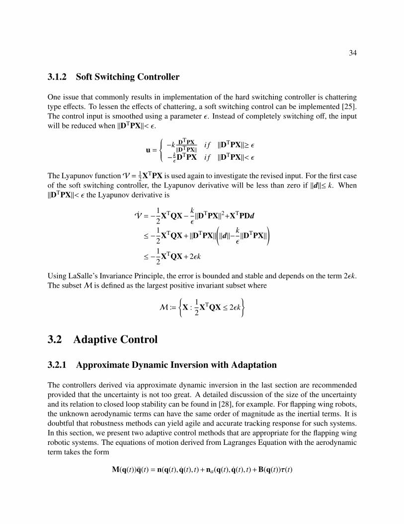
3.1.2 Soft Switching Controller
One issue that commonly results in implementation of the hard switching controller is chatteringtype effects. To lessen the effects of chattering, a soft switching control can be implemented [25].The control input is smoothed using a parameter ε. Instead of completely switching off, the inputwill be reduced when ||DTPX||< ε.
u =
−k DTPX||DTPX||
i f ||DTPX||≥ ε− kεDTPX i f ||DTPX||< ε
The Lyapunov functionV = 12XTPX is used again to investigate the revised input. For the first case
of the soft switching controller, the Lyapunov derivative will be less than zero if ||d||≤ k. When||DTPX||< ε the Lyapunov derivative is
V = −12
XTQX−kε||DTPX||2+XTPDd
≤ −12
XTQX + ||DTPX||(||d||−
kε||DTPX||
)≤ −
12
XTQX + 2εk
Using LaSalle’s Invariance Principle, the error is bounded and stable and depends on the term 2εk.The subsetM is defined as the largest positive invariant subset where
MB
X :
12
XTQX ≤ 2εk
3.2 Adaptive Control
3.2.1 Approximate Dynamic Inversion with Adaptation
The controllers derived via approximate dynamic inversion in the last section are recommendedprovided that the uncertainty is not too great. A detailed discussion of the size of the uncertaintyand its relation to closed loop stability can be found in [28], for example. For flapping wing robots,the unknown aerodynamic terms can have the same order of magnitude as the inertial terms. It isdoubtful that robustness methods can yield agile and accurate tracking response for such systems.In this section, we present two adaptive control methods that are appropriate for the flapping wingrobotic systems. The equations of motion derived from Lagranges Equation with the aerodynamicterm takes the form
M(q(t))q(t) = n(q(t), q(t), t) + na(q(t), q(t), t) + B(q(t))τ(t)
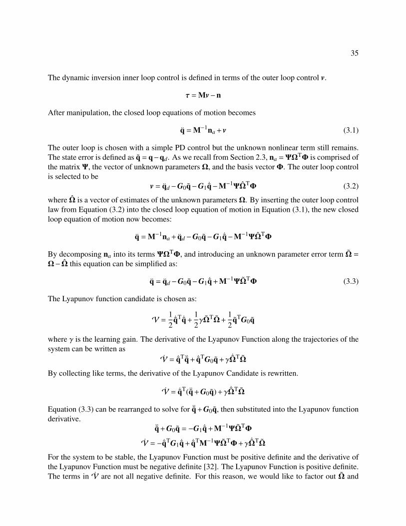
35
The dynamic inversion inner loop control is defined in terms of the outer loop control v.
τ = Mv−n
After manipulation, the closed loop equations of motion becomes
q = M−1na + v (3.1)
The outer loop is chosen with a simple PD control but the unknown nonlinear term still remains.The state error is defined as q = q−qd. As we recall from Section 2.3, na =ΨΩTΦ is comprised ofthe matrix Ψ, the vector of unknown parameters Ω, and the basis vectorΦ. The outer loop controlis selected to be
v = qd −G0q−G1 ˙q−M−1ΨΩTΦ (3.2)
where Ω is a vector of estimates of the unknown parametersΩ. By inserting the outer loop controllaw from Equation (3.2) into the closed loop equation of motion in Equation (3.1), the new closedloop equation of motion now becomes:
q = M−1na + qd −G0q−G1 ˙q−M−1ΨΩTΦ
By decomposing na into its terms ΨΩTΦ, and introducing an unknown parameter error term Ω =
Ω− Ω this equation can be simplified as:
q = qd −G0q−G1 ˙q + M−1ΨΩTΦ (3.3)
The Lyapunov function candidate is chosen as:
V =12
˙qT ˙q +12γΩTΩ+
12
qTG0q
where γ is the learning gain. The derivative of the Lyapunov Function along the trajectories of thesystem can be written as
V = ˙qT ¨q + ˙qTG0q +γ ˙ΩTΩ
By collecting like terms, the derivative of the Lyapunov Candidate is rewritten.
V = ˙qT( ¨q + G0q) +γ ˙ΩTΩ
Equation (3.3) can be rearranged to solve for ¨q + G0q, then substituted into the Lyapunov functionderivative.
¨q + G0q = −G1 ˙q + M−1ΨΩTΦ
V = − ˙qTG1 ˙q + ˙qTM−1ΨΩTΦ+γ ˙ΩTΩ
For the system to be stable, the Lyapunov Function must be positive definite and the derivative ofthe Lyapunov Function must be negative definite [32]. The Lyapunov Function is positive definite.The terms in V are not all negative definite. For this reason, we would like to factor out Ω and

36
cancel the other terms. We consider a case where the aerodynamic forces act only on a single body,i.e. Ω and Φ are column and row vectors. With this assumption, ΩTΦ ≡ΦTΩ and we can write
V = − ˙qTG1 ˙q + ( ˙qTM−1ΨΦT +γ ˙ΩT)Ω
The derivative of the unknown parameter error ˙Ω = − ˙Ω since Ω is constant. By solving for ˙Ω theupdate law is defined.
˙qTM−1ΨΦT +γ ˙ΩT = 0˙Ω = γ−1ΦΨTM−1 ˙q
A positive definite Lyapunov functionV and negative semi-definite Lyapunov derivative V guar-antees boundedness for q, ˙q, and Ω. Since ˙q is negative definite in V and positive definite inV, itis guaranteed to converge.
3.2.2 Dissipative Controller with Adaptation
To improve performance and guarantee asymptotic stability in both the position and derivativeerror, a dissipative controller is investigated. The equation of motion is rewritten with the nonlinearterm n broken down into the Coriolis matrix C and the gradient of the potential energy ∂V
∂q
M(q(t))q(t) + C(q(t), ˙q(t)) +∂V∂q(t)
−na(q(t), q(t), t) = B(q(t))τ(t) (3.4)
A new measure of the tracking error σ is introduced with diagonal, positive gain matrix Λ:
σ = ˙q +Λq
The control input is selected as
τ = M(q)(q + σ) + C(q, q)(q +σ) +∂V∂q
+ GDσ−ΨΦTΩ
It is assumed that the actuators are revolute and B is the identity matrix. The control input issubstituted into Equation 3.4 to obtain:
M(q)(−σ) + C(q, q)(−σ)−GDσ−ΨΦT(Ω− Ω) = 0
M(q)σ+ C(q, q)σ+ GDσ+ΨΦTΩ = 0 (3.5)
A Lyapunov function candidate is chosen to examine stability. The Lyapunov function, and itsderivative along the system trajectories, are expressed in the form
V =12σTM(q)σ+ qTΛGDq +
12ΩTGΩΩ
V =σTM(q)σ+ 2qTΛGD ˙q + ˙ΩTGΩΩ+12σTMσ (3.6)

37
Equation (3.5) is solved for M(q)σ and substituted into the Lyapunov derivative in Equation (3.6).
V =σT(−C(q, q)−GDσ−ΨΦTΩ) + 2qTΛGD ˙q + ˙ΩTGΩΩ+
12σTMσ
=12σT(M(q)−2C(q, q))σ−σTGDσ−σ
TΨΦTΩ+ 2qTΛGD ˙q + ˙ΩTGΩΩ
The first term is equal to zero since the matrix M(q)−2C(q, q) is skew symmetric. The derivativeof the Lyapunov function can now be written in the form
V =− ˙qTGD ˙q−2qTΛGD ˙q− qTΛGDΛq + ( ˙ΩTGΩ−σTΨΦT)Ω+ 2qTΛGD ˙q
=− ˙qTGD ˙q− qTΛGDΛq + ( ˙ΩTGΩ−σTΨΦT)Ω
When we choose the learning update law
˙ΩTGΩ−σTΨΦT = 0
˙Ω =G−1Ω ΦΨ
Tσ
˙Ω =−G−1Ω ΦΨ
Tσ
The gain matrix GΩ is square and symmetric so it is equal to its transpose GTΩ
= GΩ. The terms im-ply the Lyapunov derivative is negative semi-definite, which means that σ, Ω, and q are bounded.We also infer that both ˙q and q approach zero asymptotically because their terms in V are negativedefinite.
3.3 Numerical Simulation
3.3.1 Software Architecture
The closed loop simulations on the Adaptive Dynamic Inversion Controller and Adaptive Dissipa-tive Controller were run using MATLAB and Simulink. The software architecture is partitionedinto two main sections, Coriolis4DOF Daedalus and Fundx. Coriolis4DOF Daedalus is a top levelMATLAB script responsible for creating the linear in parameter matrices used as the precursor forthe next section. This includes the mass matrix, nonlinear Coriolis matrix, and potential energygradient. Computing these matrices every iteration in the main simulation would increase run timesignificantly.Figure (3.1) shows the entire user defined file hierarchy for the Coriolis4DOF Daedalus file. Theoutput of this code is the three elements connected to the external data symbol. The first level offunctions are DHKineticEnergy, DHPotentialEnergy, and LagrangesCoriolis. DHKineticEnergyinputs the DH parameters, symbolic velocities names, link types, center of mass vectors, masses,and inertia values. The symbolic, scalar kinetic energy value and symbolic mass matrix are the

38
outputs. The output is similar as those listed in Appendix (A.1) but with masses m1 through m4and all the inertia terms are numerically evaluated. The inputs for DHPotentialEnergy are theDH parameters, local mass locations, and masses, and the output is the Potential Energy term V .Lastly, the inputs for LagrangesCoriolis are the kinetic and potential energies and the outputs arethe Coriolis matrix and potential energy gradient.DHKineticEnergy calls three children, DHJacobianVelocity, DHInertiaMatrix, and DHJacobianOmega.The translational velocity Jacobian Jv and angular velocity Jacobian Jω are generated with the DH-JacobianVelocity and DHJacobianOmega functions, respectively. DHInertiaMatrix generates theInertia Matrix I used in the calculation of the rotational mass matrix component: Mω
i =(Jωi
)TIiJωi .
These three children and DHPotentialEnergy call DHTransforms, which generates the homoge-neous transform H for each link.
Fundx
Coriolis4DOF_Daedalus
DHKineticEnergy DHPotentialEnergy LagrangesCoriolis
Mass Matrix
Coriolis Matrix
Potential Energy Gradient
DHJacobianVelocity DHInertiaMatrix DHJacobianOmega
DHTransforms
Figure 3.1: Coriolis4DOF code hierarchy
The main execution of the simulation is titled Fundx. The data extracted from Coriolis4DOF Daedalusis copied as text into Fundx before runtime. Fundx is run as an Interpreted MATLAB Function inSimulink where it is given initial conditions and integrated. The Simulink solver ODE 113 wasselected for all cases. See Figure (3.2) for the Fundx Simulink block diagram. The inputs and out-puts to Fundx are tabulated in Table (3.1). The inputs are denoted as the column vector x and theoutput is the column vector derivative dx. The example in the table uses the closed loop equationof motion and update law from the Dissipative controller simulation. In this example, the heightof x would be 81 units, where there is one for time, four for q, four for q, and 72 for the entireparameter estimation vector Ω.The user defined hierarchy for Fundx is illustrated in Figure (3.3). Fundx has seven immediate chil-dren in this hierarchy. The first child is the function DHCalcAlphaBetaWind. This function inputs

39
Table 3.1: Fundx input and output for dissipative controller simulationInput, x Output, dx Descriptiont 1 Time counterq q Velocity obtained from inputq q = qd −Λ ˙q + M−1
(Cσ+ GDσ+ΨΦTΩ
)Closed Loop Equation of Motion
Ω ˙Ω = GΩΦΨTσ Update Law
the generalized coordinates q, constant DH parameters, wind vector vw, link types, aerodynamiccenters, and aerodynamic rotation matrices RB
0 . DHCalcAlphaBetaWind calculates the angle ofattack αi, sideslip βi, and velocity at aerodynamic center vai . The next child is SBRotation, whichgenerates the Rotation Matrix RS i
Biusing angle of attack and sideslip. PsiRestructure is a child of
Fundx which generates the 3×2N matrix to structure Ψ with the correct dimensions with input N.The child function Hat generates a linear regression basis function at the specific angle of attack,location of the hat function, and mesh spacing. This is used in the construction ofΦ. The last threedirect subfunctions of Fundx are qdesired, dqdesired, and ddqdesired. These three functions call asecond level subfunction qdqddq desired which returns the desired functions, desired derivatives,and desired double derivatives. Fundx lastly calculates the variables in dx listed in Table (3.1).
Figure 3.2: Fundx Simulink diagram, with signal dimension displayed

40
Fundx
DHCalcAlphaBetaWind SBRotation PsiRestructure qdesired dqdesired ddqdesiredHat
DHJacobianVelocity DHTransforms
DHTransforms
qdqddq_desired
Mass Matrix
Coriolis Matrix
Potential Energy GradientCoriolis4DOF_Daedalus
Figure 3.3: Fundx code hierarchy
3.3.2 Dynamic Inversion Controller
Several simulations were performed in Simulink to verify the various control designs. To begin, asimple model was run using the dynamic inversion controller with adaptation. The joint structure ismodeled after the Daedalus wing design. The mass matrix was used as described in Section 2.4 andAppendix A.1. The DH parameters are re-listed below. For this simulation, only the second bodywas assumed to generate lift. All other aerodynamic forces on the robotic system were neglected.The aerodynamic centers for all the bodies are listed along with the aerodynamic rotation matrixRB2
2 .
RB22 :
0 −1 00 0 −11 0 0
The basis functions used in the adaptive controller are a set of piecewise linear functions. This firstsimulation used nine functions to approximate cL(αi). The range, step size, and true parameters are
Table 3.2: Daedalus DH parameters used in dynamic inversion simulationLink di(m) ai(m) θi(rad) αi(rad)1 0.1 0 θ1
π2
2 0 0.1 θ2 03 0 0.1 θ3 04 0 0.1 θ4 0

41
Table 3.3: Daedalus relative aerodynamic centers, riai
Linkx coordi-nate (m)
y coordi-nate (m)
z coordi-nate (m)
1 0 0 02 -0.05 0 -0.053 0 -0.05 04 -0.05 0 0
listed below. The true parameters used in this simulation are based on experimental results froman S 1223 airfoil [1, 33].
Angle of Attack Range (degrees):[−22.5 22.5
]Angle of Attack Step Size (degrees):
[5.625
]Ω =
[−0.5 −0.3 −0.2 0.05 1.1 1.6 1.95 2.22 1.9
]
Using these true parameters and the basis functions, the true cL graph is generated and depicted inFigure 3.4. The separate basis functions that compose the cL curve are plotted in Figure (3.5). The
−25 −20 −15 −10 −5 0 5 10 15 20 25−0.5
0
0.5
1
1.5
2
2.5
angle of attack (deg)
true
cL
appr
oxim
atio
n
Figure 3.4: True cL curve used in the numerical studies
wing area for body 2 is selected to be 1m2 constant wind vector vw = −5y0 m/s. The gravitationalconstant is chosen as g = 9.81 m/s and the air density is chosen as ρ = 1.2 kg/m3. The controller

42
−25 −20 −15 −10 −5 0 5 10 15 20 25−0.5
0
0.5
1
1.5
2
2.5
angle of attack (degrees)
mag
nitu
de
Figure 3.5: True cL curve decomposed into the nine separate basis functions
gains are set as
G0 :
50 0 0 00 50 0 00 0 50 00 0 0 50
G1 :
50 0 0 00 50 0 00 0 50 00 0 0 50
γ :
[1000
]
Periodic functions are used to drive θ2 and θ3 which represent the flapping motion observed inbirds. The desired joint angle histories are chosen as follows:
θ2,d =Asin(ωt)
θ3,d =−Asin(ωt +
π
2
)−A
where A is the amplitude andω is the flapping frequency. A frequency ofω= 3 Hz and amplitude ofA = 15 is reasonable for mimicking birds on the larger end of the range in the Larus genus [3, 4].An illustrative example of the desired flapping motion is pictured in Figure (3.6). In the two
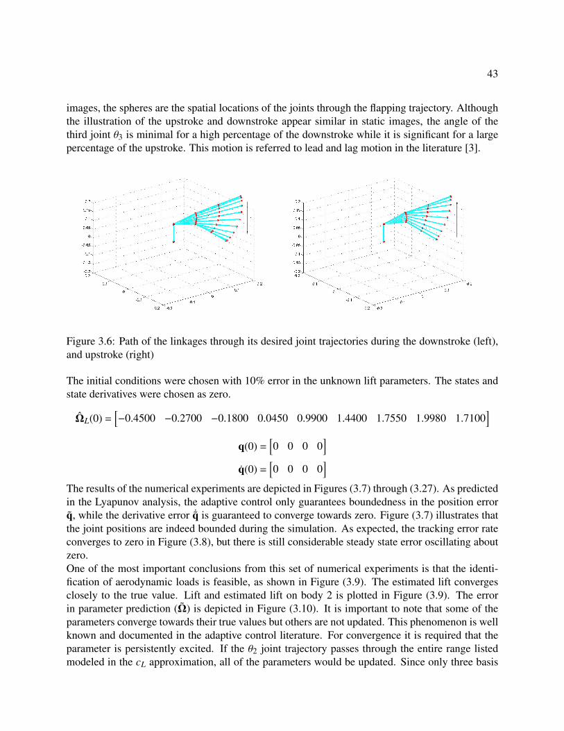
43
images, the spheres are the spatial locations of the joints through the flapping trajectory. Althoughthe illustration of the upstroke and downstroke appear similar in static images, the angle of thethird joint θ3 is minimal for a high percentage of the downstroke while it is significant for a largepercentage of the upstroke. This motion is referred to lead and lag motion in the literature [3].
Figure 3.6: Path of the linkages through its desired joint trajectories during the downstroke (left),and upstroke (right)
The initial conditions were chosen with 10% error in the unknown lift parameters. The states andstate derivatives were chosen as zero.
ΩL(0) =[−0.4500 −0.2700 −0.1800 0.0450 0.9900 1.4400 1.7550 1.9980 1.7100
]q(0) =
[0 0 0 0
]q(0) =
[0 0 0 0
]The results of the numerical experiments are depicted in Figures (3.7) through (3.27). As predictedin the Lyapunov analysis, the adaptive control only guarantees boundedness in the position errorq, while the derivative error ˙q is guaranteed to converge towards zero. Figure (3.7) illustrates thatthe joint positions are indeed bounded during the simulation. As expected, the tracking error rateconverges to zero in Figure (3.8), but there is still considerable steady state error oscillating aboutzero.One of the most important conclusions from this set of numerical experiments is that the identi-fication of aerodynamic loads is feasible, as shown in Figure (3.9). The estimated lift convergesclosely to the true value. Lift and estimated lift on body 2 is plotted in Figure (3.9). The errorin parameter prediction (Ω) is depicted in Figure (3.10). It is important to note that some of theparameters converge towards their true values but others are not updated. This phenomenon is wellknown and documented in the adaptive control literature. For convergence it is required that theparameter is persistently excited. If the θ2 joint trajectory passes through the entire range listedmodeled in the cL approximation, all of the parameters would be updated. Since only three basis

44
0 1 2 3 4 5 6 7 8 9 10−0.6
−0.4
−0.2
0
0.2
0.4
0.6
0.8
1
time (s)
posi
tion
erro
rs (
rad)
θ
1
θ2
θ3
θ4
Figure 3.7: Errors in joint positions with lift acting on body 2
function ranges are visited, and for differing amounts of time, the error decreases most rapidly inthe range from −5.625
to +5.625
. Less change is made to parameters ranging −11.25
to 0
and0
to 11.25
. The angle of attack of body 2 is plotted in Figure (3.11). This simulation provides agood indication of which parameters update and converge during the simulation.The next numerical experiment considers both drag and lift on bodies 2 through 4. The true valuesof lift remain unchained from the previous experiment for all of the wing bodies. A separate setof nine parameters were chosen to model the true cD(αi) function. The DH parameters, mass vari-ables, aerodynamic center locations, angle of attack step size and range, wind vector, air densityand gravitational constant were not changed. The aerodynamic rotation matrices were updated toinclude all of the bodies.
RB11 :
0 −1 00 0 −11 0 0
RB22 :
0 −1 00 0 −11 0 0
RB3
3 :
0 −1 00 0 −11 0 0
RB44 :
0 −1 00 0 −11 0 0
The wing areas were updated to account for the wing areas among the last three bodies. The firstbody was omitted by choosing the area to be zero. The result is a simulation in which lift and dragare generated only the wing sections, where the first body has minimal aerodynamic effects on thesystem by comparison. Shifting the area towards the root, such as on link 2, will increase lift whileadding less significantly to the control effort than on body 3 or 4. The wing areas were reselected

45
0 1 2 3 4 5 6 7 8 9 10−5
−4
−3
−2
−1
0
1
2
3
time (s)
velo
city
err
ors
(rad
/s)
θ1
θ2
θ3
θ4
Figure 3.8: Errors in joint velocities
to generate similar magnitudes of lift from the previous experiment.
Wing areas(m2) :[0 0.25 0.1 0.05
]The true unknown parameters are the coefficients that multiply the nine functions used to representthe drag and lift on each body. The true drag parameter, as in the case of the true lift coefficients,were selected to model experimental data for an S1223 airfoil. Some values for large negativeangles of attack were interpolated from the data to choose values for the true unknown parametersand graph which exceeded −6. The drag function cD generated by the true parameters appears inFigure (3.12).
Ω =
ΩD1
ΩL1...ΩD4
ΩL4
=
0.5 0.3 0.13 0.08 0.04 0.05 0.1 0.2 0.4−0.5 −0.3 −0.2 0.05 1.1 1.6 1.95 2.22 1.90.5 0.3 0.13 0.08 0.04 0.05 0.1 0.2 0.4−0.5 −0.3 −0.2 0.05 1.1 1.6 1.95 2.22 1.90.5 0.3 0.13 0.08 0.04 0.05 0.1 0.2 0.4−0.5 −0.3 −0.2 0.05 1.1 1.6 1.95 2.22 1.90.5 0.3 0.13 0.08 0.04 0.05 0.1 0.2 0.4−0.5 −0.3 −0.2 0.05 1.1 1.6 1.95 2.22 1.9
The initial conditions were repeated from the first experiment with 10% error in each body for bothlift and drag.
ΩL(0) =[−0.4500 −0.2700 −0.1800 0.0450 0.9900 1.4400 1.7550 1.9980 1.7100
]

46
0 1 2 3 4 5 6 7 8 9 103
4
5
6
7
8
9
10
11
time (s)
lift o
n bo
dy 2
(N
)
L2
L2
Figure 3.9: Lift on body 2 and estimated lift on body 2
ΩD(0) =[0.4500 0.2700 0.1170 0.0720 0.0360 0.0450 0.0900 0.1800 0.3600
]The learning gain was tuned lower than the single body simulation, which effectively raises thelearning rate. The other control gains remained unchanged.
G0 :
. . .
50. . .
G1 :
. . .
50. . .
γ :
[100
]
After modifying the unknown aerodynamic model to include multiple wing bodies, the results ofthe numerical experiment are depicted in Figures (3.13) through (3.16). The joint position errorsillustrated in Figure (3.13) are qualitatively similar to that in the single body case. The magnitudeof errors in joint velocities, shown in Figure (3.14) were also in the same range as in the singlebody simulation. The new drag forces on the system increased the magnitude of the response of θ1and θ1 since these forces caused a torque about the θ1 axis due to the direction of the wind.The parameter errors vary between each wing segment as seen in Figure (3.15). Body 1 has nolearning during the simulation since its area is set to zero. As expected, the parameters associated

47
0 1 2 3 4 5 6 7 8 9 10−0.25
−0.2
−0.15
−0.1
−0.05
0
0.05
0.1
time (s)
unkn
own
para
met
er e
rror
Figure 3.10: Parameter error on body 2 lift
with body 4 exhibit the most learning throughout the trial since its angle of attack varies the mostcompared to the other links. See Figure (3.16) for the graphs of angle of attack in this simulation.Body 2 undergoes a smaller fluctuation in angle of attack, resulting in smaller aerodynamic forces,and consequently its associated parameters do not update as frequently. Since convergence ofthe parameter error is not guaranteed by the controller, it is expected that not all parameters willconverge towards zero. Some of the parameters affiliated with the highest and lowest angle ofattack are not modified by the update law. Specifically, 14 parameters are affected by the updatelaw in the fourth body, 10 parameters in the third body, and six parameters in the second body.

48
0 1 2 3 4 5 6 7 8 9 10−3
−2
−1
0
1
2
3
4
time (s)
angl
e of
atta
ck o
f bod
y 2
(deg
)
Figure 3.11: Angle of attack of body 2
−25 −20 −15 −10 −5 0 5 10 15 20 250
0.05
0.1
0.15
0.2
0.25
0.3
0.35
0.4
0.45
0.5
angle of attack (deg)
true
cD
app
roxi
mat
ion
Figure 3.12: True cD curve using nine unknown functions

49
0 1 2 3 4 5 6 7 8 9 10−0.3
−0.2
−0.1
0
0.1
0.2
0.3
0.4
0.5
0.6
time (s)
posi
tion
erro
rs (
rad)
θ
1
θ2
θ3
θ4
Figure 3.13: Errors in joint positions with drag and lift acting on bodies 2−4
0 1 2 3 4 5 6 7 8 9 10−5
−4
−3
−2
−1
0
1
2
time (s)
velo
city
err
ors
(rad
/s)
θ1
θ2
θ3
θ4
Figure 3.14: Errors in joint velocities with drag and lift acting on bodies 2−4

50
0 2 4 6 8 10−0.25
−0.2
−0.15
−0.1
−0.05
0
0.05
0.1
time (s)
body
1 p
aram
eter
err
or
0 2 4 6 8 10−0.4
−0.3
−0.2
−0.1
0
0.1
0.2
0.3
time (s)
body
2 p
aram
eter
err
or
0 2 4 6 8 10−0.25
−0.2
−0.15
−0.1
−0.05
0
0.05
0.1
time (s)
body
3 p
aram
eter
err
or
0 2 4 6 8 10−0.25
−0.2
−0.15
−0.1
−0.05
0
0.05
0.1
time (s)
body
4 p
aram
eter
err
or
Figure 3.15: Parameter errors on bodies 1−4
0 1 2 3 4 5 6 7 8 9 10−20
−15
−10
−5
0
5
10
15
20
time (s)
sngl
e of
stta
ck o
f bod
ies
(deg
)
α1α2α3α4
Figure 3.16: Angle of attack for wing sections 1−4

51
3.3.3 Dissipative Controller
The dissipative controller discussed in Section (3.2.2) was compared in this section with the adap-tive dynamic inversion controller. The numerical experiment is based on the mass and DH param-eters for the Daedalus model as listed in the previous section. The aerodynamic rotation matrices,wing areas, and true unknown parameters were not changed from the second dynamic inversioncontroller. New gains were selected for the controller, including the gains GΩ, Λ, and GD. Thegains were chosen on basis for low settling error with less weight on settling time.
GΩ :
. . .
50. . .
Λ :
. . .
1. . .
GD :
. . .
1. . .
The controller shows improved performance in comparison to the dynamic inversion controller.Both the joint position errors, in Figure (3.17), and joint velocity errors, in Figure (3.18), convergequickly. The 5% settling time of all the transients depicted in Figures (3.17) and (3.18) is less than2.985 seconds. The control input torques associated with these gains is pictured in Figure (3.19).There is a high initial transient in two of the input torques, but soon after there is a steady periodicresponse. The peak input torques for joints 2 and 3 were higher than the other two input torques,but were not excessive. The maximum control input for τ3 is 1.5 N·m and τ2 has a maximummagnitude of 3.852 N·m. For comparison, the Dynamixel RX-24F servomotor used in the Larusprototype has a stall torque of 2.6 N·m. Gearing can be used to increase the torque at the sacrificeof angular velocity.The update law in the dissipative controller appears to work more smoothly than the previouscontroller. The unknown parameter errors plotted in Figure (3.20) decrease exponentially towardzero for most of the parameters. Some examples of excited parameters are the third and fourth liftparameter of body 2, in Figures (3.21) and (3.22), respectively. Again, non-convergence of someof the parameters can be understood in terms of persistency of excitation of the angle of attack.The number of parameters updated effectively in the simulation remains unchanged from that ofthe previous controller, with six parameters in Body 2, 10 parameters in Body 3, and 14 parametersin Body 4. Figure (3.23) shows the similarity of the angle of attack responses to the angle of attackresponse in the dynamic inversion controller.The lift function is pictured in Figure (3.24). With the chosen wing sizes and wind velocity the lift
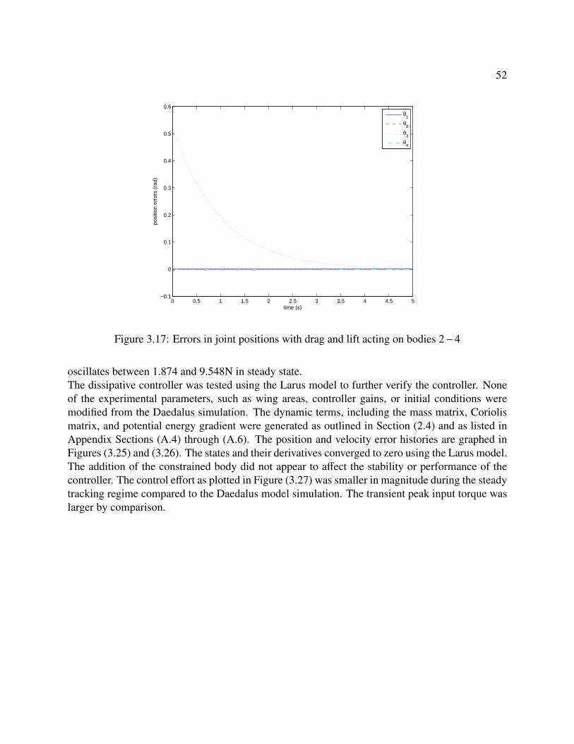
52
0 0.5 1 1.5 2 2.5 3 3.5 4 4.5 5−0.1
0
0.1
0.2
0.3
0.4
0.5
0.6
time (s)
posi
tion
erro
rs (
rad)
θ
1
θ2
θ3
θ4
Figure 3.17: Errors in joint positions with drag and lift acting on bodies 2−4
oscillates between 1.874 and 9.548N in steady state.The dissipative controller was tested using the Larus model to further verify the controller. Noneof the experimental parameters, such as wing areas, controller gains, or initial conditions weremodified from the Daedalus simulation. The dynamic terms, including the mass matrix, Coriolismatrix, and potential energy gradient were generated as outlined in Section (2.4) and as listed inAppendix Sections (A.4) through (A.6). The position and velocity error histories are graphed inFigures (3.25) and (3.26). The states and their derivatives converged to zero using the Larus model.The addition of the constrained body did not appear to affect the stability or performance of thecontroller. The control effort as plotted in Figure (3.27) was smaller in magnitude during the steadytracking regime compared to the Daedalus model simulation. The transient peak input torque waslarger by comparison.

53
0 0.5 1 1.5 2 2.5 3 3.5 4 4.5 5−5
−4
−3
−2
−1
0
1
time (s)
velo
city
err
ors
(rad
/s)
θ1
θ2
θ3
θ4
Figure 3.18: Errors in joint velocities with drag and lift acting on bodies 2−4
0 0.1 0.2 0.3 0.4 0.5 0.6 0.7 0.8 0.9 1−4
−3
−2
−1
0
1
2
3
time (s)
cont
rol i
nput
(N
−m
)
Figure 3.19: Dissipative controller effort on bodies 2−4

54
0 1 2 3 4 5−0.25
−0.2
−0.15
−0.1
−0.05
0
0.05
0.1
body
1 p
aram
eter
err
or
0 1 2 3 4 5−0.4
−0.2
0
0.2
0.4
0.6
0.8
1
body
2 p
aram
eter
err
or
0 1 2 3 4 5−0.4
−0.3
−0.2
−0.1
0
0.1
0.2
0.3
body
3 p
aram
eter
err
or
0 1 2 3 4 5−0.25
−0.2
−0.15
−0.1
−0.05
0
0.05
0.1
body
4 p
aram
eter
err
or
Figure 3.20: Parameter error on bodies 1−4 in the dissipative controller simulation
0 0.5 1 1.5 2 2.5 3 3.5 4 4.5 5−0.4
−0.3
−0.2
−0.1
0
0.1
0.2
0.3
time (s)
para
met
er e
rror
Figure 3.21: Error of the third lift parameter of body 2
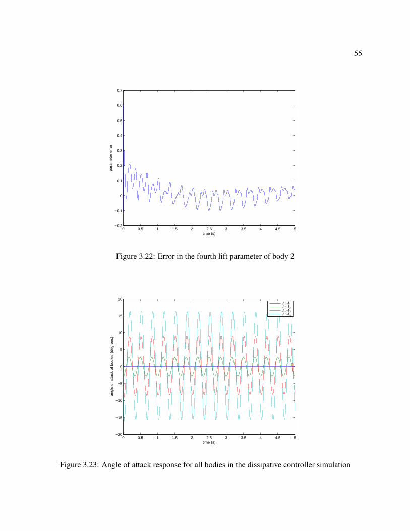
55
0 0.5 1 1.5 2 2.5 3 3.5 4 4.5 5−0.2
−0.1
0
0.1
0.2
0.3
0.4
0.5
0.6
0.7
time (s)
para
met
er e
rror
Figure 3.22: Error in the fourth lift parameter of body 2
0 0.5 1 1.5 2 2.5 3 3.5 4 4.5 5−20
−15
−10
−5
0
5
10
15
20
time (s)
angl
e of
atta
ck o
f bod
ies
(deg
rees
)
AoA1
AoA2
AoA3
AoA4
Figure 3.23: Angle of attack response for all bodies in the dissipative controller simulation
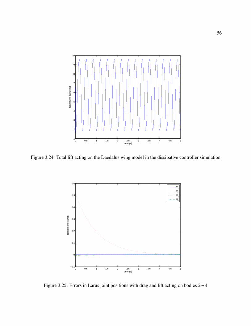
56
0 0.5 1 1.5 2 2.5 3 3.5 4 4.5 51
2
3
4
5
6
7
8
9
10
time (s)
tota
l lift
on
bodi
es(N
)
Figure 3.24: Total lift acting on the Daedalus wing model in the dissipative controller simulation
0 0.5 1 1.5 2 2.5 3 3.5 4 4.5 5−0.1
0
0.1
0.2
0.3
0.4
0.5
0.6
time (s)
posi
tion
erro
rs (
rad)
θ
1
θ2
θ3
θ4
Figure 3.25: Errors in Larus joint positions with drag and lift acting on bodies 2−4

57
0 0.5 1 1.5 2 2.5 3 3.5 4 4.5 5−5
−4
−3
−2
−1
0
1
time (s)
velo
city
err
ors
(rad
/s)
θ1
θ2
θ3
θ4
Figure 3.26: Errors in Larus joint velocities with drag and lift acting on bodies 2−4
0 0.1 0.2 0.3 0.4 0.5 0.6 0.7 0.8 0.9 1−2
−1
0
1
2
3
4
time (s)
cont
rol i
nput
(N
−m
)
Figure 3.27: Dissipative controller effort on bodies 2−4 using the Larus dynamic model

Chapter 4
Conclusion
This thesis has studied two classes of flapping wing robot models. One is a kinematic and dynamicmodel of systems with a fixed base body. The kinematic and dynamic models for the fixed basecase are constructed using techniques applicable to kinematic chains. The kinematic descriptionemployed for these type of robotic systems are available in standard robotics texts [24–26]. Usingthe Denavit-Hartenberg convention and analytical mechanics, the mass matrix, Coriolis matrix,and potential energy gradient are generated for the Daedalus and Larus models. These terms areused to build the open loop equations of motion. This thesis introduces a method for calculatingthe contributions of the aerodynamic lift and drag forces to the robotic equations of motion. Thegeneralized equations of motion are then written in the form
M(q(t))q(t) = n(q(t), q(t), t) + na(q(t), q(t), t) + B(q(t))τ(t) (4.1)
where M is the mass matrix, n is the nonlinear term that arise in the robot dynamics, na is thenonlinear term that appear when the aerodynamics are considered, and B is the control influencematrix. These equations differ from standard textbook models of robotic systems. Two types ofadaptive nonlinear controllers are developed for creating the closed loop equations of motion forthe fixed body case. The first is a dynamic inversion controller with adaptation. The second is adissipative controller with adaptation. A Lyapunov analysis demonstrates that the dynamic inver-sion controller will ensure that the joint tracking error rates converge towards zero, but the jointposition errors are only guaranteed to be bounded. Numerical experiments based on MathworksSimulink have been carried out to verify the Lyapunov analysis of stability and convergence. Thesimulation also demonstrates that the adaptive control is able to learn parameters that determinethe aerodynamic loads when they are persistently excited.The dissipative controller was studied to improve performance in comparison to the first controller.Both the joint position and velocity errors are guaranteed to diminish to zero from the Lyapunovanalysis. The simulation for this model again verified the Lyapunov analysis. Within the first fiveseconds of the numerical experiment for this controller, the maximum velocity and position steadystate error was below 0.7% of the initial position error and 0.1% of the initial velocity error, re-spectively. With the gains set to yield a maximum control effort of 3.85 N·m, the position settled
58

59
in 2.98 seconds to within 5% of the initial error. The development of a new robotic bird prototypewill aid in verification of the numerical simulation.
4.1 Future Work
Several novel directions of study are suggested by the research carried out in this thesis. The nu-merical experiments in the thesis do not include tests of robustness to external disturbances, suchas a time varying wind vector. Robustness of the control methodology to such external effects maybe an important factor in the performance of the adaptive controller and should be studied in de-tail. The numerical experiments also did not model any uncertainty in parameters such as masses,lengths, center of mass locations, etc. Only uncertainty in the aerodynamic loads has been studied.The combined effect of uncertainty in model parameters (such as link length, mass, mass centerlocation) and in aerodynamic load should be investigated. Another important and fundamental lim-itation of the strategy outlined in this paper is the selection of a quasi steady aerodynamic model inthe controller. It is well-known that the flow surrounding flapping wings is unsteady, and nonlinear.More realistic flow models should be studied.The third flapping wing prototype Icarus is proposed to finish completion before May 2013. Tocombine the efforts of the control design and aircraft design, a new kinematic model needs to bedeveloped based on the new structure featured in Icarus. More importantly, the moving base bodydynamic model and control design need to be extended so that they are applicable to a flying vehi-cle such as Icarus. The nonlinear aerodynamic term needs to be re-evaluated to model the effectsof the aerodynamics on the whole flapping flight system, including the base body. This thesis doesnot include the steps for generating the various Jacobian matrices used to relate the base body todifferent chain bases or the ground frame.The control design for the moving base body dynamic model will be a complex problem, onethat has not been directly addressed in literature. The adaptive control and learning theory shouldbe developed further to better model the aerodynamics and increase robustness. In the imme-diate future, the development of an L1 controller with an “adaptive basis” will be investigatedand simulated using the existing dynamic model. Furthermore, the aerodynamic model could beadvanced simultaneously with the adaptive controller to result in a highly robust controller. Aslightweight and compact on board hardware processing evolves over the next decade or more,complex unsteady aerodynamics models could perhaps be implemented in a real time algorithmusing a microcontroller or microprocessing unit.

Bibliography
[1] M.S. Selig and J.J. Guglielmo. High-Lift Low Reynolds Number Airfoil Design. Journal ofAircraft, 34, 1997.
[2] T. Liu, K. Kuykendoll, R. Rhew, and S. Jones. Avian Wing Geometry and Kinematics. AIAAJournal, 47, 2006.
[3] Cheolheui Han. Investigation of Unsteady Aerodynamic Characteristics of a Seagull Wingin Level Flight. Journal of Bionic Engineering, 6, 2009.
[4] K. Scoley. Developments in Vertibrate Flight, Climbing and Gliding of Mammals andReplites, and The Flapping Flight of Birds. PhD thesis, University of Bristol, 1982.
[5] K. Aditya and V. Malolan. Investigation of Strouhal Number effect on flapping wing microair vehicle. AIAA Paper, 2007.
[6] D. Mueller, H.A. Bruck, and S.K. Gupta. Measurement of thrust and lift forces associatedwith drag of compliant flapping wing for micro air vehicles using a new test stand design.Experimental Mechanics, 50:725–735, 2010.
[7] K.D. Ellenrieder, K. Parker, and J. Soria. Fluid Mechanics of Flapping Wings. ExperimentalThermal and Fluid Science, 32, 2008.
[8] X. Deng, L. Schenato, and S.S. Sastry. Flapping Flight for Biomimetic Robotic Insects: PartII-Flight Control Design. IEEE Transactions on Robotics, 22:789–802, 2006.
[9] X. Deng, L. Schenato, W. Wu, and S.S. Sastry. Flapping Flight for Biomimetic RoboticInsects: Part I-System Modeling. IEEE Transactions on Robotics, 22:789–802, 2006.
[10] S.A. Ansari, R. Zbikowski, and K. Knowles. Aerodynamics Modelling of Insect-Like Flap-ping Flight for Micro Air Vehicles. Progress in Aerospace Sciences, 42:129–172, 2006.
[11] B. Singh and I. Chopra. Insect Based Hover-Capable Flapping Wings for Micro Air Vehicles:Experiments and Analysis. AIAA Journal, 46:2115–2135, 2008.
[12] G. Bunget and S. Seelecke. BATMAV: a 2-DOF Bio-Inspired Flapping Flight Platform.Active and Passive Smart Structures and Integrated Systems, 7643:1–10, 2010.
60
61
[13] K. Miklasz, M. LaBarbera, X. Chen, and J.J. Socha. Effects of Body Cross-sectional Shapeon Flying Snake Aerodynamics. Experimental Mechanics, 2010.
[14] J.J. Socha. Gliding Flight in Chrysopelea: Turning a Snake into a Wing. Integrative andComparative Biology, 51:969–982, 2011.
[15] J.J. Socha, T. O’Dempsey, and M. LaBarbera. A 3-d kinematic analysis of gliding in flyingsnake, chrysopelea paradisi. Journal of Experimental Biology, 208, 2005.
[16] K. Sibilski, J. Pietrucha, and M. Zlocka. The comparative evaluation of power requirementsfor fixed, rotary, and flapping wings micro air vehicles. AIAA Paper, 2007.
[17] G.K. Taylor and A.L.R. Thomas. Animal Flight Dynamics II. Longitudal Stability in FlappingFlight. Journal of Theoretical Biology, 214:351–370, 2002.
[18] B.Y. Leonard. Flapping wing flight dynamic modeling. Master’s thesis, Virginia PolytechnicInstitute and State University, 2011.
[19] P. Gopalakrishnan and D.K. Tafti. Effect of Rotation Kinematics and Angle of Attack onFlapping Flight. AIAA Journal, 47:2505–2519, 2009.
[20] K. Mazaheri and A Ebrahimi. Experiment Investigation on Aerodynamic Performance of aFlapping Wing Vehicle in Forward Flight. Journal of Fluids and Structures, 27:586–595,2011.
[21] A. Muniappa, V. Baskar, and V. Duriyanandhan. Lift and thrust characteristics of flappingwing micro air vehicle (MAV). AIAA Paper, 2011.
[22] G.K. Taylor, R.L. Nudds, and A.L.R. Thomas. Flying and swimming animals cruise at astrouhal number tuned for high power efficiency. Nature, pages 707–711, 2003.
[23] K. Crandell and B. Tobalske. Aerodynamics of tip-reversal upstroke in a revolving pigeonwing. The Journal of Experimental Biology, 214, 2011.
[24] M.W. Spong, S. Hutchinson, and M. Vidyasagar. Robot Modeling and Control. John Wiley& Sons, Inc., Hoboken, New Jersey, 2006.
[25] A. J. Kurdila, A. Leonessa, and J. Vignola. Dynamics and Control of Robotic Systems.Springer, New York City, New York, 2012.
[26] B. Siciliano, L. Sciavicco, L. Villani, and G. Oriolo. Robotics Modeling, Planning and Con-trol. Springer-Verlag London Limited, London, UK, 2009.
[27] L. Meirovitch. Dynamics and Control of Structures. John Wiley & Sons, Inc., Hoboken, NewJersey, 1990.
[28] F.L. Lewis, C.T. Abdallah, and D.M. Dawson. Control Of Robot Manipulators. MaxwellMacmillan Publishing Co., Oxford, UK, 1993.

62
[29] S. Beutel, A. Dupont, G. Hofmeister, I. Hyun, J. Bayandor, and A. Kurdila. Daedalus: AFresh Bio-Inspired Aircraft Design Concept. In 50th AIAA Aerospace Sciences Meeting,Nashville, TN, January 2012.
[30] E. Fisher, A. Bauhofer, C. Beauchene, B. Dress, S. Marshall, C. McCraw, C. Mehrvarzi,C. Ng, J. Simcic, J. Bayandor, and A. Kurdila. A Bio-Inspired Aircraft Design Concept. InProceedings of the ASME 2012 Fluids Engineering Division Summer Meeting, Rio Grande,Puerto Rico, July 2012.
[31] J. Feaster, A. Golding, E. Guerra, K. Lukesch, A. Matta, T. Suh, D. Volk, J. Witte, J. Bayan-dor, and A. Kurdila. On Design and Analysis of Larus Genus Inspired Biomimetic Aircraft.Blacksburg, VA, May 2013.
[32] J.E. Slotine and W. Li. Applied Nonlinear Control. Prentice Hall, Englewood Cliffs, NewJersey, 1991.
[33] R. Ma and P. Liu. Numerical Simulation of Low-Reynolds-Number and High-Lift Airfoils1223. Proceedings of the World Congress on Engineering, 2, 2009.

Appendix A
Dynamic Model Examples
A.1 Daedalus Mass Matrix
m(1,1) = [I1,yy + I3,xy sin(2θ2 + 2θ3) + I4,yy cos(θ2 + θ3 + θ4)2 + I4,xx sin(θ2 + θ3 + θ4)2 + (m3(cos(θ2 +
θ3) + 2cos(θ2))2)/400 + I3,yy cos(θ2 + θ3)2 + m2(cos(2θ2)/800 + 1/800) + I3,xx sin(θ2 + θ3)2 +
I2,yy cos(θ2)2 +(m4(cos(θ2 +θ3 +θ4)+2cos(θ2 +θ3)+2cos(θ2))2)/400+ I2,xy sin(2θ2)+ I2,xx sin(θ2)2 +
I4,xy sin(2θ2 + 2θ3 + 2θ4)]
m(1,2) = [I3,yz cos(θ2 + θ3) + I3,xz sin(θ2 + θ3) + I2,yz cos(θ2) + I2,xz sin(θ2) + I4,yz cos(θ2 + θ3 + θ4) +
I4,xz sin(θ2 + θ3 + θ4)]
m(1,3) = [I3,yz cos(θ2 + θ3) + I3,xz sin(θ2 + θ3) + I4,yz cos(θ2 + θ3 + θ4) + I4,xz sin(θ2 + θ3 + θ4)]
m(1,4) = [I4,yz cos(θ2 + θ3 + θ4) + I4,xz sin(θ2 + θ3 + θ4)]
m(2,1) = [I3,yz cos(θ2 + θ3) + I3,xz sin(θ2 + θ3) + I2,yz cos(θ2) + I2,xz sin(θ2) + I4,yz cos(θ2 + θ3 + θ4) +
I4,xz sin(θ2 + θ3 + θ4)]
m(2,2) = [I1,zz + I3,zz + I4,zz + m2/400 + m3/80 + (9m4)/400 + (m4 cos(θ3 + θ4))/100 +
(m3 cos(θ3))/100 + (m4 cos(θ3))/50 + (m4 cos(θ4))/100]
m(2,3) = [I3,zz + I4,zz + m3/400 + m4/80 + (m4 cos(θ3 + θ4))/200 + (m3 cos(θ3))/200 +
(m4 cos(θ3))/100 + (m4 cos(θ4))/100]
m(2,4) = [I4,zz + m4/400 + (m4 cos(θ3 + θ4))/200 + (m4 cos(θ4))/200]
m(3,1) = [I3,yz cos(θ2 + θ3) + I3,xz sin(θ2 + θ3) + I4,yz cos(θ2 + θ3 + θ4) + I4,xz sin(θ2 + θ3 + θ4)]
63

64
m(3,2) = [I3,zz + I4,zz + m3/400 + m4/80 + (m4 cos(θ3 + θ4))/200 + (m3 cos(θ3))/200 +
(m4 cos(θ3))/100 + (m4 cos(θ4))/100]
m(3,3) = [I3,zz + I4,zz + m3/400 + m4/80 + (m4 cos(θ4))/100]
m(3,4) = [I4,zz + m4/400 + (m4 cos(θ4))/200]
m(4,1) = [I4,yz cos(θ2 + θ3 + θ4) + I4,xz sin(θ2 + θ3 + θ4)]
m(4,2) = [I4,zz + m4/400 + (m4 cos(θ3 + θ4))/200 + (m4 cos(θ4))/200]
m(4,3) = [I4,zz + m4/400 + (m4 cos(θ4))/200]
m(4,4) = [I4,zz + m4/400]
A.2 Daedalus Nonlinear Coriolis Matrix
C(1,1) = [θ2(I3,xy cos(2θ2 + 2θ3)− (m2 sin(2θ2))/800 + (I3,xx sin(2θ2 + 2θ3))/2− (I3,yy sin(2θ2 +
2θ3))/2 + I2,xy cos(2θ2) + I4,xy cos(2θ2 + 2θ3 + 2θ4) + (I2,xx sin(2θ2))/2− (I2,yy sin(2θ2))/2 +
(I4,xx sin(2θ2 + 2θ3 + 2θ4))/2− (I4,yy sin(2θ2 + 2θ3 + 2θ4))/2− (m3(cos(θ2 + θ3) + 2cos(θ2))(sin(θ2 +
θ3) + 2sin(θ2)))/400− (m4(cos(θ2 + θ3 + θ4) + 2cos(θ2 + θ3) + 2cos(θ2))(sin(θ2 + θ3 + θ4) + 2sin(θ2 +
θ3) + 2sin(θ2)))/400) + θ3(I3,xy cos(2θ2 + 2θ3) + (I3,xx sin(2θ2 + 2θ3))/2 − (I3,yy sin(2θ2 + 2θ3))/2 +
I4,xy cos(2θ2 +2θ3 +2θ4)+ (I4,xx sin(2θ2 +2θ3 +2θ4))/2− (I4,yy sin(2θ2 +2θ3 +2θ4))/2− (m4(sin(θ2 +
θ3 + θ4) +
2sin(θ2 + θ3))(cos(θ2 + θ3 + θ4) + 2cos(θ2 + θ3) + 2cos(θ2)))/400 − (m3 sin(θ2 + θ3)(cos(θ2 + θ3) +
2cos(θ2)))/400) +
θ4(I4,xy cos(2θ2 +2θ3 +2θ4)+ (I4,xx sin(2θ2 +2θ3 +2θ4))/2− (I4,yy sin(2θ2 +2θ3 +2θ4))/2− (m4 sin(θ2+ θ3 + θ4)(cos(θ2 + θ3 + θ4) + 2cos(θ2 + θ3) + 2cos(θ2)))/400)]
C(1,2) = [θ1(I3,xy cos(2θ2 + 2θ3)− (m2 sin(2θ2))/800 + (I3,xx sin(2θ2 + 2θ3))/2− (I3,yy sin(2θ2+ 2θ3))/2 + I2,xy cos(2θ2) + I4,xy cos(2θ2 + 2θ3 + 2θ4) + (I2,xx sin(2θ2))/2−(I2,yy sin(2θ2))/2 + (I4,xx sin(2θ2 + 2θ3 + 2θ4))/2− (I4,yy sin(2θ2 + 2θ3 + 2θ4))/2− (m3(cos(θ2 + θ3) +
2cos(θ2))(sin(θ2 + θ3) + 2sin(θ2)))/400− (m4(cos(θ2 + θ3 + θ4) + 2cos(θ2 + θ3) + 2cos(θ2))(sin(θ2 +
θ3 +θ4)+2sin(θ2 +θ3)+2sin(θ2)))/400)+ θ3(I3,xz cos(θ2 +θ3)− I3,yz sin(θ2 +θ3)+ I4,xz cos(θ2 +θ3 +
θ4)− I4,yz sin(θ2 + θ3 + θ4)) + θ2(I3,xz cos(θ2 + θ3)− I3,yz sin(θ2 + θ3) + I2,xz cos(θ2)− I2,yz sin(θ2) +
I4,xz cos(θ2 + θ3 + θ4)− I4,yz sin(θ2 + θ3 + θ4)) + θ4(I4,xz cos(θ2 + θ3 + θ4)− I4,yz sin(θ2 + θ3 + θ4))]
C(1,3) = [θ1(I3,xy cos(2θ2 + 2θ3) + (I3,xx sin(2θ2 + 2θ3))/2− (I3,yy sin(2θ2 + 2θ3))/2 + I4,xy cos(2θ2 +
2θ3 + 2θ4) + (I4,xx sin(2θ2 + 2θ3 + 2θ4))/2 − (I4,yy sin(2θ2 + 2θ3 + 2θ4))/2 − (m4(sin(θ2 + θ3 + θ4) +
2sin(θ2 + θ3))(cos(θ2 + θ3 + θ4) + 2cos(θ2 + θ3) + 2cos(θ2)))/400 − (m3 sin(θ2 + θ3)(cos(θ2 + θ3) +

65
2cos(θ2)))/400) + θ2(I3,xz cos(θ2 + θ3)− I3,yz sin(θ2 + θ3) + I4,xz cos(θ2 + θ3 + θ4)− I4,yz sin(θ2 + θ3 +
θ4)) + θ3(I3,xz cos(θ2 + θ3)− I3,yz sin(θ2 + θ3) + I4,xz cos(θ2 + θ3 + θ4)− I4,yz sin(θ2 + θ3 + θ4)) +
θ4(I4,xz cos(θ2 + θ3 + θ4)− I4,yz sin(θ2 + θ3 + θ4))]
C(1,4) = [θ1(I4,xy cos(2θ2 +2θ3 +2θ4)+ (I4,xx sin(2θ2 +2θ3 +2θ4))/2− (I4,yy sin(2θ2 +2θ3 +2θ4))/2−(m4 sin(θ2 + θ3 + θ4)(cos(θ2 + θ3 + θ4) + 2cos(θ2 + θ3) + 2cos(θ2)))/400) + θ2(I4,xz cos(θ2 + θ3 + θ4)−I4,yz sin(θ2 + θ3 + θ4)) + θ3(I4,xz cos(θ2 + θ3 + θ4)− I4,yz sin(θ2 + θ3 + θ4)) + θ4(I4,xz cos(θ2 + θ3 + θ4)−I4,yz sin(θ2 + θ3 + θ4))]
C(2,1) = [(I2,yyθ1 sin(2θ2))/2− I4,xyθ1 cos(2θ2 + 2θ3 + 2θ4)− (I2,xxθ1 sin(2θ2))/2− I2,xyθ1 cos(2θ2)−(I4,xxθ1 sin(2θ2 + 2θ3 + 2θ4))/2 + (I4,yyθ1 sin(2θ2 + 2θ3 + 2θ4))/2− I3,xyθ1 cos(2θ2 + 2θ3) +
(θ1m2 sin(2θ2))/800− (I3,xxθ1 sin(2θ2 + 2θ3))/2 + (I3,yyθ1 sin(2θ2 + 2θ3))/2 + (θ1m3(cos(θ2 + θ3) +
s2cos(θ2))(sin(θ2 +θ3)+2sin(θ2)))/400+(θ1m4(cos(θ2 +θ3 +θ4)+2cos(θ2 +θ3)+2cos(θ2))(sin(θ2 +
θ3 + θ4) + 2sin(θ2 + θ3) + 2sin(θ2)))/400]
C(2,2) = [−θ3((m4 sin(θ3 +θ4))/200+(m3 sin(θ3))/200+(m4 sin(θ3))/100)− θ4((m4 sin(θ3 +θ4))/200+ (m4 sin(θ4))/200)]
C(2,3) = [−θ2((m4 sin(θ3 +θ4))/200+(m3 sin(θ3))/200+(m4 sin(θ3))/100)− θ3((m4 sin(θ3 +θ4))/200+ (m3 sin(θ3))/200 + (m4 sin(θ3))/100)− θ4((m4 sin(θ3 + θ4))/200 + (m4 sin(θ4))/200)]
C(2,4) = [−(m4(sin(θ3 + θ4) + sin(θ4))(θ2 + θ3 + θ4))/200]
C(3,1) = [(I4,yyθ1 sin(2θ2 + 2θ3 + 2θ4))/2− (I4,xxθ1 sin(2θ2 + 2θ3 + 2θ4))/2− I4,xyθ1 cos(2θ2 + 2θ3 +
2θ4)− I3,xyθ1 cos(2θ2 + 2θ3)− (I3,xxθ1 sin(2θ2 + 2θ3))/2 + (I3,yyθ1 sin(2θ2 + 2θ3))/2 + (θ1m3 sin(θ2 +
θ3)(cos(θ2 +θ3)+2cos(θ2)))/400+(θ1m4(sin(θ2 +θ3 +θ4)+2sin(θ2 +θ3))(cos(θ2 +θ3 +θ4)+2cos(θ2+ θ3) + 2cos(θ2)))/400]
C(3,2) = [θ2((m4 sin(θ3 + θ4))/200 + (m3 sin(θ3))/200 + (m4 sin(θ3))/100)− (θ4m4 sin(θ4))/200]
C(3,3) = [−(θ4m4 sin(θ4))/200]
C(3,4) = [−(m4 sin(θ4)(θ2 + θ3 + θ4))/200]
C(4,1) = [(I4,yyθ1 sin(2θ2 + 2θ3 + 2θ4))/2− (I4,xxθ1 sin(2θ2 + 2θ3 + 2θ4))/2− I4,xyθ1 cos(2θ2 + 2θ3 +
2θ4) + (θ1m4 sin(θ2 + θ3 + θ4)(cos(θ2 + θ3 + θ4) + 2cos(θ2 + θ3) + 2cos(θ2)))/400]
C(4,2) = [θ2((m4 sin(θ3 + θ4))/200 + (m4 sin(θ4))/200) + (θ3m4 sin(θ4))/200]
C(4,3) = [(m4 sin(θ4)(θ2 + θ3))/200]
C(4,4) = [0]
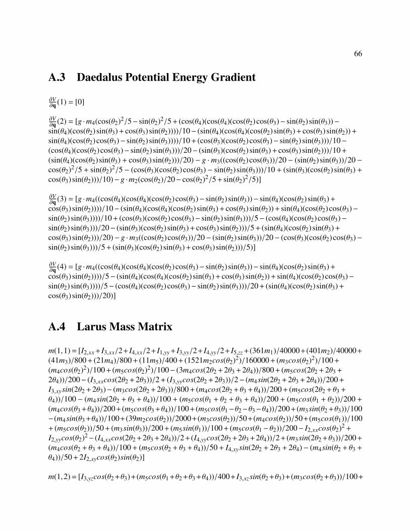
66
A.3 Daedalus Potential Energy Gradient
∂V∂q (1) = [0]
∂V∂q (2) = [g ·m4(cos(θ2)2/5− sin(θ2)2/5 + (cos(θ4)(cos(θ4)(cos(θ2)cos(θ3)− sin(θ2) sin(θ3))−sin(θ4)(cos(θ2) sin(θ3) + cos(θ3) sin(θ2))))/10− (sin(θ4)(cos(θ4)(cos(θ2) sin(θ3) + cos(θ3) sin(θ2)) +
sin(θ4)(cos(θ2)cos(θ3)− sin(θ2) sin(θ3))))/10 + (cos(θ3)(cos(θ2)cos(θ3)− sin(θ2) sin(θ3)))/10−(cos(θ4)(cos(θ2)cos(θ3)− sin(θ2) sin(θ3)))/20− (sin(θ3)(cos(θ2) sin(θ3) + cos(θ3) sin(θ2)))/10 +
(sin(θ4)(cos(θ2) sin(θ3) + cos(θ3) sin(θ2)))/20) − g ·m3((cos(θ2)cos(θ3))/20 − (sin(θ2) sin(θ3))/20 −cos(θ2)2/5 + sin(θ2)2/5 − (cos(θ3)(cos(θ2)cos(θ3) − sin(θ2) sin(θ3)))/10 + (sin(θ3)(cos(θ2) sin(θ3) +
cos(θ3) sin(θ2)))/10)−g ·m2(cos(θ2)/20− cos(θ2)2/5 + sin(θ2)2/5)]
∂V∂q (3) = [g ·m4((cos(θ4)(cos(θ4)(cos(θ2)cos(θ3)− sin(θ2) sin(θ3))− sin(θ4)(cos(θ2) sin(θ3) +
cos(θ3) sin(θ2))))/10− (sin(θ4)(cos(θ4)(cos(θ2) sin(θ3) + cos(θ3) sin(θ2)) + sin(θ4)(cos(θ2)cos(θ3)−sin(θ2) sin(θ3))))/10 + (cos(θ3)(cos(θ2)cos(θ3)− sin(θ2) sin(θ3)))/5− (cos(θ4)(cos(θ2)cos(θ3)−sin(θ2) sin(θ3)))/20− (sin(θ3)(cos(θ2) sin(θ3) + cos(θ3) sin(θ2)))/5 + (sin(θ4)(cos(θ2) sin(θ3) +
cos(θ3) sin(θ2)))/20)− g ·m3((cos(θ2)cos(θ3))/20− (sin(θ2) sin(θ3))/20− (cos(θ3)(cos(θ2)cos(θ3)−sin(θ2) sin(θ3)))/5 + (sin(θ3)(cos(θ2) sin(θ3) + cos(θ3) sin(θ2)))/5)]
∂V∂q (4) = [g ·m4((cos(θ4)(cos(θ4)(cos(θ2)cos(θ3)− sin(θ2) sin(θ3))− sin(θ4)(cos(θ2) sin(θ3) +
cos(θ3) sin(θ2))))/5− (sin(θ4)(cos(θ4)(cos(θ2) sin(θ3) + cos(θ3) sin(θ2)) + sin(θ4)(cos(θ2)cos(θ3)−sin(θ2) sin(θ3))))/5− (cos(θ4)(cos(θ2)cos(θ3)− sin(θ2) sin(θ3)))/20 + (sin(θ4)(cos(θ2) sin(θ3) +
cos(θ3) sin(θ2)))/20)]
A.4 Larus Mass Matrix
m(1,1) = [I2,xx + I3,xx/2+ I4,xx/2+ I1,yy + I3,yy/2+ I4,yy/2+ I5,zz +(361m1)/40000+(401m2)/40000+
(41m3)/800 + (21m4)/800 + (11m5)/400 + (1521m2cos(θ2)2)/160000 + (m3cos(θ2)2)/100 +
(m4cos(θ2)2)/100 + (m5cos(θ2)2)/100− (3m4cos(2θ2 + 2θ3 + 2θ4))/800 + (m5cos(2θ2 + 2θ3 +
2θ4))/200− (I3,xxcos(2θ2 + 2θ3))/2 + (I3,yycos(2θ2 + 2θ3))/2− (m4sin(2θ2 + 2θ3 + 2θ4))/200 +
I3,xysin(2θ2 + 2θ3)− (m3cos(2θ2 + 2θ3))/800 + (m4cos(2θ2 + θ3 + θ4))/200 + (m5cos(2θ2 + θ3 +
θ4))/100 − (m4sin(2θ2 + θ3 + θ4))/100 + (m5cos(θ1 + θ2 + θ3 + θ4))/200 + (m5cos(θ1 + θ2))/200 +
(m4cos(θ3 +θ4))/200+ (m5cos(θ3 +θ4))/100+ (m5cos(θ1−θ2−θ3−θ4))/200+ (m3sin(θ2 +θ3))/100−(m4sin(θ3 +θ4))/100+(39m2cos(θ2))/2000+(m3cos(θ2))/50+(m4cos(θ2))/50+(m5cos(θ1))/100+ (m5cos(θ2))/50 + (m3sin(θ3))/200 + (m5sin(θ1))/100 + (m5cos(θ1− θ2))/200− I2,xxcos(θ2)2 +
I2,yycos(θ2)2− (I4,xxcos(2θ2 +2θ3 +2θ4))/2+ (I4,yycos(2θ2 +2θ3 +2θ4))/2+ (m3sin(2θ2 +θ3))/200+
(m4cos(θ2 + θ3 + θ4))/100 + (m5cos(θ2 + θ3 + θ4))/50 + I4,xysin(2θ2 + 2θ3 + 2θ4)− (m4sin(θ2 + θ3 +
θ4))/50 + 2I2,xycos(θ2)sin(θ2)]
m(1,2) = [I3,yzcos(θ2 +θ3)+(m5cos(θ1 +θ2 +θ3 +θ4))/400+ I3,xzsin(θ2 +θ3)+(m3cos(θ2 +θ3))/100+

67
(m5cos(θ1 + θ2))/400 − (m5cos(θ1 − θ2 − θ3 − θ4))/400 + I2,yzcos(θ2) − I5,yzcos(θ1) + I2,xzsin(θ2) +
I5,xzsin(θ1) + (39m2sin(θ2))/80000− (m3sin(θ2))/50− (m4sin(θ2))/100− (m5sin(θ2))/100 +
I4,yzcos(θ2 + θ3 + θ4)− (m5cos(θ1 − θ2))/400 + I4,xzsin(θ2 + θ3 + θ4)− (m4cos(θ2 + θ3 + θ4))/100−(m4sin(θ2 + θ3 + θ4))/200− (m5sin(θ2 + θ3 + θ4))/100]
m(1,3) = [I3,yzcos(θ2 +θ3)+(m5cos(θ1 +θ2 +θ3 +θ4))/400+ I3,xzsin(θ2 +θ3)+(m3cos(θ2 +θ3))/100−(m5cos(θ1− θ2− θ3− θ4))/400− I5,yzcos(θ1) + I5,xzsin(θ1) + I4,yzcos(θ2 + θ3 + θ4) + I4,xzsin(θ2 + θ3 +
θ4)− (m4cos(θ2 + θ3 + θ4))/100− (m4sin(θ2 + θ3 + θ4))/200− (m5sin(θ2 + θ3 + θ4))/100]
m(1,4) = [(m5cos(θ1 + θ2 + θ3 + θ4))/400− (m5cos(θ1 − θ2 − θ3 − θ4))/400 + I4,yzcos(θ2 + θ3 + θ4) +
I4,xzsin(θ2 + θ3 + θ4)− (m4cos(θ2 + θ3 + θ4))/100− (m4sin(θ2 + θ3 + θ4))/200− (m5sin(θ2 + θ3 +
θ4))/100]
m(2,1) = [I3,yzcos(θ2 +θ3)+(m5cos(θ1 +θ2 +θ3 +θ4))/400+ I3,xzsin(θ2 +θ3)+(m3cos(θ2 +θ3))/100+
(m5cos(θ1 + θ2))/400 − (m5cos(θ1 − θ2 − θ3 − θ4))/400 + I2,yzcos(θ2) − I5,yzcos(θ1) + I2,xzsin(θ2) +
I5,xzsin(θ1) + (39m2sin(θ2))/80000− (m3sin(θ2))/50− (m4sin(θ2))/100− (m5sin(θ2))/100 +
I4,yzcos(θ2 + θ3 + θ4)− (m5cos(θ1 − θ2))/400 + I4,xzsin(θ2 + θ3 + θ4)− (m4cos(θ2 + θ3 + θ4))/100−(m4sin(θ2 + θ3 + θ4))/200− (m5sin(θ2 + θ3 + θ4))/100]
m(2,2) = [I1,zz + I3,zz + I4,zz + (1521m2)/160000 + m3/80 + (9m4)/400 + m5(sin(θ2 + θ3 + θ4)/10 +
sin(θ2)/10)2 + (m4cos(θ3 + θ4))/100 + m5(cos(θ2 + θ3 + θ4)/10 + cos(θ1)/20 + cos(θ2)/10)2−
(m4sin(θ3 + θ4))/50 + cos(θ1)(I5,yycos(θ1)− I5,xysin(θ1)) + (m3sin(θ3))/100− sin(θ1)(I5,xycos(θ1)−I5,xxsin(θ1))]
m(2,3) = [I5,xx/2 + I5,yy/2 + I3,zz + I4,zz + m3/400 + m4/80 + (9m5)/800 + (m5cos(2θ1))/800 +
(m5cos(θ1 +θ2 +θ3 +θ4))/200+(m5cos(θ1 +θ2))/400+(m4cos(θ3 +θ4))/200+(m5cos(θ3 +θ4))/100+ (m5cos(θ1−θ2−θ3−θ4))/200− (m4sin(θ3 +θ4))/100+ (m3sin(θ3))/200+ (m5cos(θ1−θ2))/400−(I5,xxcos(2θ1))/2 + (I5,yycos(2θ1))/2− I5,xysin(2θ1)]
m(2,4) = [I4,zz +m4/80+m5/100+(m5cos(θ1 +θ2 +θ3 +θ4))/400+(m4cos(θ3 +θ4))/200+(m5cos(θ3+ θ4))/100 + (m5cos(θ1− θ2− θ3− θ4))/400− (m4sin(θ3 + θ4))/100]
m(3,1) = [I3,yzcos(θ2 +θ3)+(m5cos(θ1 +θ2 +θ3 +θ4))/400+ I3,xzsin(θ2 +θ3)+(m3cos(θ2 +θ3))/100−(m5cos(θ1− θ2− θ3− θ4))/400− I5,yzcos(θ1) + I5,xzsin(θ1) + I4,yzcos(θ2 + θ3 + θ4) + I4,xzsin(θ2 + θ3 +
θ4)− (m4cos(θ2 + θ3 + θ4))/100− (m4sin(θ2 + θ3 + θ4))/200− (m5sin(θ2 + θ3 + θ4))/100]
m(3,2) = [I5,xx/2 + I5,yy/2 + I3,zz + I4,zz + m3/400 + m4/80 + (9m5)/800 + (m5cos(2θ1))/800 +
(m5cos(θ1 +θ2 +θ3 +θ4))/200+(m5cos(θ1 +θ2))/400+(m4cos(θ3 +θ4))/200+(m5cos(θ3 +θ4))/100+ (m5cos(θ1−θ2−θ3−θ4))/200− (m4sin(θ3 +θ4))/100+ (m3sin(θ3))/200+ (m5cos(θ1−θ2))/400−(I5,xxcos(2θ1))/2 + (I5,yycos(2θ1))/2− I5,xysin(2θ1)]
m(3,3) = [I5,xx/2 + I5,yy/2 + I3,zz + I4,zz + m3/400 + m4/80 + (9m5)/800 +

68
(m5cos(2θ1))/800 + (m5cos(θ1 + θ2 + θ3 + θ4))/200 + (m5cos(θ1− θ2− θ3− θ4))/200−(I5,xxcos(2θ1))/2 + (I5,yycos(2θ1))/2− I5,xysin(2θ1)]
m(3,4) = [I4,zz + m4/80 + m5/100 + (m5cos(θ1 + θ2 + θ3 + θ4))/400 + (m5cos(θ1− θ2− θ3− θ4))/400]
m(4,1) = [(m5cos(θ1 + θ2 + θ3 + θ4))/400− (m5cos(θ1 − θ2 − θ3 − θ4))/400 + I4,yzcos(θ2 + θ3 + θ4) +
I4,xzsin(θ2 + θ3 + θ4)− (m4cos(θ2 + θ3 + θ4))/100− (m4sin(θ2 + θ3 + θ4))/200− (m5sin(θ2 + θ3 +
θ4))/100]
m(4,2) = [I4,zz +m4/80+m5/100+(m5cos(θ1 +θ2 +θ3 +θ4))/400+(m4cos(θ3 +θ4))/200+(m5cos(θ3+ θ4))/100 + (m5cos(θ1− θ2− θ3− θ4))/400− (m4sin(θ3 + θ4))/100]
m(4,3) = [I4,zz + m4/80 + m5/100 + (m5cos(θ1 + θ2 + θ3 + θ4))/400 + (m5cos(θ1− θ2− θ3− θ4))/400]
m(4,4) = [I4,zz + m4/80 + m5/100]
A.5 Larus Nonlinear Coriolis Matrix
C(1,1) = [−θ3((m4 cos(2θ2 +2θ3 +2θ4))/200− I3,xy cos(2θ2 +2θ3)− (3m4 sin(2θ2 +2θ3 +2θ4))/800+
(m5 sin(2θ2 + 2θ3 + 2θ4))/200− (I3,xx sin(2θ2 + 2θ3))/2 + (I3,yy sin(2θ2 + 2θ3))/2− (m3 sin(2θ2 +
2θ3))/800+ (m4 cos(2θ2 +θ3 +θ4))/200+ (m4 sin(2θ2 +θ3 +θ4))/400+ (m5 sin(2θ2 +θ3 +θ4))/200+
(m5 sin(θ1 +θ2 +θ3 +θ4))/400−(m3 cos(θ2 +θ3))/200+(m4 cos(θ3 +θ4))/200+(m4 sin(θ3 +θ4))/400+(m5 sin(θ3 +θ4))/200−(m5 sin(θ1−θ2−θ3−θ4))/400−(m3 cos(θ3))/400−(m3 cos(2θ2 +θ3))/400−I4,xy cos(2θ2 +2θ3 +2θ4)+ (m4 cos(θ2 +θ3 +θ4))/100− (I4,xx sin(2θ2 +2θ3 +2θ4))/2+ (I4,yy sin(2θ2 +
2θ3 + 2θ4))/2 + (m4 sin(θ2 + θ3 + θ4))/200 + (m5 sin(θ2 + θ3 + θ4))/100)− θ2((m4 cos(2θ2 + 2θ3 +
2θ4))/200− I3,xy cos(2θ2 +2θ3)+(1521m2 sin(2θ2))/320000+(m3 sin(2θ2))/200+(m4 sin(2θ2))/200+(m5 sin(2θ2))/200−(3m4 sin(2θ2 +2θ3 +2θ4))/800+(m5 sin(2θ2 +2θ3 +2θ4))/200−(I3,xx sin(2θ2 +
2θ3))/2+(I3,yy sin(2θ2 +2θ3))/2−(m3 sin(2θ2 +2θ3))/800+(m4 cos(2θ2 +θ3 +θ4))/100+(m4 sin(2θ2+θ3 +θ4))/200+(m5 sin(2θ2 +θ3 +θ4))/100+(m5 sin(θ1 +θ2 +θ3 +θ4))/400−(m3 cos(θ2 +θ3))/200+
(m5 sin(θ1 + θ2))/400 − (m5 sin(θ1 − θ2 − θ3 − θ4))/400 + (39m2 sin(θ2))/4000 + (m3 sin(θ2))/100 +
(m4 sin(θ2))/100 + (m5 sin(θ2))/100− (m3 cos(2θ2 + θ3))/200− I2,xy cos(2θ2)− I4,xy cos(2θ2 + 2θ3 +
2θ4)− (m5 sin(θ1− θ2))/400 + (m4 cos(θ2 + θ3 + θ4))/100− (I2,xx sin(2θ2))/2 + (I2,yy sin(2θ2))/2−(I4,xx sin(2θ2 +2θ3 +2θ4))/2+ (I4,yy sin(2θ2 +2θ3 +2θ4))/2+ (m4 sin(θ2 +θ3 +θ4))/200+ (m5 sin(θ2 +
θ3 + θ4))/100)− θ4((m4 cos(2θ2 + 2θ3 + 2θ4))/200− (3m4 sin(2θ2 + 2θ3 + 2θ4))/800 + (m5 sin(2θ2 +
2θ3 + 2θ4))/200 + (m4 cos(2θ2 + θ3 + θ4))/200 + (m4 sin(2θ2 + θ3 + θ4))/400 + (m5 sin(2θ2 + θ3 +
θ4))/200+ (m5 sin(θ1 +θ2 +θ3 +θ4))/400+ (m4 cos(θ3 +θ4))/200+ (m4 sin(θ3 +θ4))/400+ (m5 sin(θ3+θ4))/200− (m5 sin(θ1−θ2−θ3−θ4))/400− I4,xy cos(2θ2 +2θ3 +2θ4)+ (m4 cos(θ2 +θ3 +θ4))/100−(I4,xx sin(2θ2 +2θ3 +2θ4))/2+ (I4,yy sin(2θ2 +2θ3 +2θ4))/2+ (m4 sin(θ2 +θ3 +θ4))/200+ (m5 sin(θ2 +
θ3 + θ4))/100) − θ1((m5 sin(θ1 + θ2 + θ3 + θ4))/400 + (m5 sin(θ1 + θ2))/400 + (m5 sin(θ1 − θ2 − θ3 −
θ4))/400− (m5 cos(θ1))/200 + (m5 sin(θ1))/200 + (m5 sin(θ1− θ2))/400)]
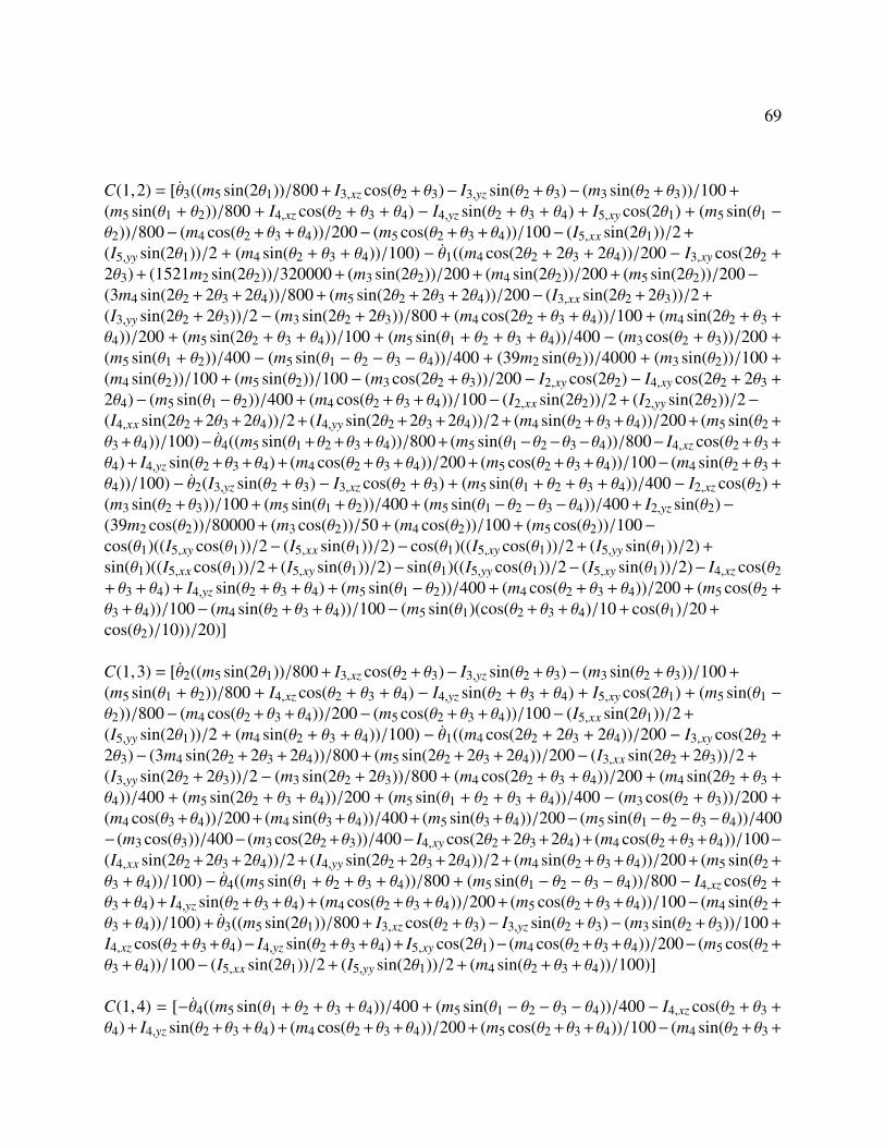
69
C(1,2) = [θ3((m5 sin(2θ1))/800 + I3,xz cos(θ2 + θ3)− I3,yz sin(θ2 + θ3)− (m3 sin(θ2 + θ3))/100 +
(m5 sin(θ1 + θ2))/800 + I4,xz cos(θ2 + θ3 + θ4) − I4,yz sin(θ2 + θ3 + θ4) + I5,xy cos(2θ1) + (m5 sin(θ1 −
θ2))/800− (m4 cos(θ2 + θ3 + θ4))/200− (m5 cos(θ2 + θ3 + θ4))/100− (I5,xx sin(2θ1))/2 +
(I5,yy sin(2θ1))/2 + (m4 sin(θ2 + θ3 + θ4))/100) − θ1((m4 cos(2θ2 + 2θ3 + 2θ4))/200 − I3,xy cos(2θ2 +
2θ3) + (1521m2 sin(2θ2))/320000 + (m3 sin(2θ2))/200 + (m4 sin(2θ2))/200 + (m5 sin(2θ2))/200−(3m4 sin(2θ2 + 2θ3 + 2θ4))/800 + (m5 sin(2θ2 + 2θ3 + 2θ4))/200− (I3,xx sin(2θ2 + 2θ3))/2 +
(I3,yy sin(2θ2 + 2θ3))/2− (m3 sin(2θ2 + 2θ3))/800 + (m4 cos(2θ2 + θ3 + θ4))/100 + (m4 sin(2θ2 + θ3 +
θ4))/200 + (m5 sin(2θ2 + θ3 + θ4))/100 + (m5 sin(θ1 + θ2 + θ3 + θ4))/400 − (m3 cos(θ2 + θ3))/200 +
(m5 sin(θ1 + θ2))/400 − (m5 sin(θ1 − θ2 − θ3 − θ4))/400 + (39m2 sin(θ2))/4000 + (m3 sin(θ2))/100 +
(m4 sin(θ2))/100 + (m5 sin(θ2))/100− (m3 cos(2θ2 + θ3))/200− I2,xy cos(2θ2)− I4,xy cos(2θ2 + 2θ3 +
2θ4)− (m5 sin(θ1− θ2))/400 + (m4 cos(θ2 + θ3 + θ4))/100− (I2,xx sin(2θ2))/2 + (I2,yy sin(2θ2))/2−(I4,xx sin(2θ2 +2θ3 +2θ4))/2+ (I4,yy sin(2θ2 +2θ3 +2θ4))/2+ (m4 sin(θ2 +θ3 +θ4))/200+ (m5 sin(θ2 +
θ3 +θ4))/100)− θ4((m5 sin(θ1 +θ2 +θ3 +θ4))/800+ (m5 sin(θ1−θ2−θ3−θ4))/800− I4,xz cos(θ2 +θ3 +
θ4)+ I4,yz sin(θ2 +θ3 +θ4)+ (m4 cos(θ2 +θ3 +θ4))/200+ (m5 cos(θ2 +θ3 +θ4))/100− (m4 sin(θ2 +θ3 +
θ4))/100)− θ2(I3,yz sin(θ2 + θ3)− I3,xz cos(θ2 + θ3) + (m5 sin(θ1 + θ2 + θ3 + θ4))/400− I2,xz cos(θ2) +
(m3 sin(θ2 + θ3))/100 + (m5 sin(θ1 + θ2))/400 + (m5 sin(θ1− θ2− θ3− θ4))/400 + I2,yz sin(θ2)−(39m2 cos(θ2))/80000 + (m3 cos(θ2))/50 + (m4 cos(θ2))/100 + (m5 cos(θ2))/100−cos(θ1)((I5,xy cos(θ1))/2− (I5,xx sin(θ1))/2)− cos(θ1)((I5,xy cos(θ1))/2 + (I5,yy sin(θ1))/2) +
sin(θ1)((I5,xx cos(θ1))/2+ (I5,xy sin(θ1))/2)− sin(θ1)((I5,yy cos(θ1))/2− (I5,xy sin(θ1))/2)− I4,xz cos(θ2+ θ3 + θ4) + I4,yz sin(θ2 + θ3 + θ4) + (m5 sin(θ1 − θ2))/400 + (m4 cos(θ2 + θ3 + θ4))/200 + (m5 cos(θ2 +
θ3 + θ4))/100− (m4 sin(θ2 + θ3 + θ4))/100− (m5 sin(θ1)(cos(θ2 + θ3 + θ4)/10 + cos(θ1)/20 +
cos(θ2)/10))/20)]
C(1,3) = [θ2((m5 sin(2θ1))/800 + I3,xz cos(θ2 + θ3)− I3,yz sin(θ2 + θ3)− (m3 sin(θ2 + θ3))/100 +
(m5 sin(θ1 + θ2))/800 + I4,xz cos(θ2 + θ3 + θ4) − I4,yz sin(θ2 + θ3 + θ4) + I5,xy cos(2θ1) + (m5 sin(θ1 −
θ2))/800− (m4 cos(θ2 + θ3 + θ4))/200− (m5 cos(θ2 + θ3 + θ4))/100− (I5,xx sin(2θ1))/2 +
(I5,yy sin(2θ1))/2 + (m4 sin(θ2 + θ3 + θ4))/100) − θ1((m4 cos(2θ2 + 2θ3 + 2θ4))/200 − I3,xy cos(2θ2 +
2θ3)− (3m4 sin(2θ2 + 2θ3 + 2θ4))/800 + (m5 sin(2θ2 + 2θ3 + 2θ4))/200− (I3,xx sin(2θ2 + 2θ3))/2 +
(I3,yy sin(2θ2 + 2θ3))/2− (m3 sin(2θ2 + 2θ3))/800 + (m4 cos(2θ2 + θ3 + θ4))/200 + (m4 sin(2θ2 + θ3 +
θ4))/400 + (m5 sin(2θ2 + θ3 + θ4))/200 + (m5 sin(θ1 + θ2 + θ3 + θ4))/400 − (m3 cos(θ2 + θ3))/200 +
(m4 cos(θ3 +θ4))/200+ (m4 sin(θ3 +θ4))/400+ (m5 sin(θ3 +θ4))/200− (m5 sin(θ1−θ2−θ3−θ4))/400−(m3 cos(θ3))/400−(m3 cos(2θ2 +θ3))/400− I4,xy cos(2θ2 +2θ3 +2θ4)+(m4 cos(θ2 +θ3 +θ4))/100−(I4,xx sin(2θ2 +2θ3 +2θ4))/2+ (I4,yy sin(2θ2 +2θ3 +2θ4))/2+ (m4 sin(θ2 +θ3 +θ4))/200+ (m5 sin(θ2 +
θ3 + θ4))/100)− θ4((m5 sin(θ1 + θ2 + θ3 + θ4))/800 + (m5 sin(θ1 − θ2 − θ3 − θ4))/800− I4,xz cos(θ2 +
θ3 +θ4)+ I4,yz sin(θ2 +θ3 +θ4)+ (m4 cos(θ2 +θ3 +θ4))/200+ (m5 cos(θ2 +θ3 +θ4))/100− (m4 sin(θ2 +
θ3 + θ4))/100) + θ3((m5 sin(2θ1))/800 + I3,xz cos(θ2 + θ3)− I3,yz sin(θ2 + θ3)− (m3 sin(θ2 + θ3))/100 +
I4,xz cos(θ2 +θ3 +θ4)− I4,yz sin(θ2 +θ3 +θ4)+ I5,xy cos(2θ1)−(m4 cos(θ2 +θ3 +θ4))/200−(m5 cos(θ2 +
θ3 + θ4))/100− (I5,xx sin(2θ1))/2 + (I5,yy sin(2θ1))/2 + (m4 sin(θ2 + θ3 + θ4))/100)]
C(1,4) = [−θ4((m5 sin(θ1 + θ2 + θ3 + θ4))/400 + (m5 sin(θ1 − θ2 − θ3 − θ4))/400− I4,xz cos(θ2 + θ3 +
θ4)+ I4,yz sin(θ2 +θ3 +θ4)+ (m4 cos(θ2 +θ3 +θ4))/200+ (m5 cos(θ2 +θ3 +θ4))/100− (m4 sin(θ2 +θ3 +

70
θ4))/100)− θ2((m5 sin(θ1 + θ2 + θ3 + θ4))/800 + (m5 sin(θ1 − θ2 − θ3 − θ4))/800− I4,xz cos(θ2 + θ3 +
θ4)+ I4,yz sin(θ2 +θ3 +θ4)+ (m4 cos(θ2 +θ3 +θ4))/200+ (m5 cos(θ2 +θ3 +θ4))/100− (m4 sin(θ2 +θ3 +
θ4))/100)− θ3((m5 sin(θ1 + θ2 + θ3 + θ4))/800 + (m5 sin(θ1 − θ2 − θ3 − θ4))/800− I4,xz cos(θ2 + θ3 +
θ4)+ I4,yz sin(θ2 +θ3 +θ4)+ (m4 cos(θ2 +θ3 +θ4))/200+ (m5 cos(θ2 +θ3 +θ4))/100− (m4 sin(θ2 +θ3 +
θ4))/100)− θ1((m4 cos(2θ2 + 2θ3 + 2θ4))/200− (3m4 sin(2θ2 + 2θ3 + 2θ4))/800 + (m5 sin(2θ2 + 2θ3 +
2θ4))/200+ (m4 cos(2θ2 +θ3 +θ4))/200+ (m4 sin(2θ2 +θ3 +θ4))/400+ (m5 sin(2θ2 +θ3 +θ4))/200+
(m5 sin(θ1 +θ2 +θ3 +θ4))/400+ (m4 cos(θ3 +θ4))/200+ (m4 sin(θ3 +θ4))/400+ (m5 sin(θ3 +θ4))/200−(m5 sin(θ1−θ2−θ3−θ4))/400− I4,xy cos(2θ2 +2θ3 +2θ4)+(m4 cos(θ2 +θ3 +θ4))/100−(I4,xx sin(2θ2+ 2θ3 + 2θ4))/2 + (I4,yy sin(2θ2 + 2θ3 + 2θ4))/2 + (m4 sin(θ2 + θ3 + θ4))/200 + (m5 sin(θ2 + θ3 +
θ4))/100)]
C(2,1) = [θ1((m4 cos(2θ2 + 2θ3 + 2θ4))/200− I3,xy cos(2θ2 + 2θ3) + (1521m2 sin(2θ2))/320000 +
(m3 sin(2θ2))/200 + (m4 sin(2θ2))/200 + (m5 sin(2θ2))/200− (3m4 sin(2θ2 + 2θ3 + 2θ4))/800 +
(m5 sin(2θ2 + 2θ3 + 2θ4))/200− (I3,xx sin(2θ2 + 2θ3))/2 + (I3,yy sin(2θ2 + 2θ3))/2− (m3 sin(2θ2 +
2θ3))/800+ (m4 cos(2θ2 +θ3 +θ4))/100+ (m4 sin(2θ2 +θ3 +θ4))/200+ (m5 sin(2θ2 +θ3 +θ4))/100−(m3 cos(θ2 + θ3))/200 + I5,xz cos(θ1) + I5,yz sin(θ1) + (39m2 sin(θ2))/4000 + (m3 sin(θ2))/100 +
(m4 sin(θ2))/100 + (m5 sin(θ2))/100− (m3 cos(2θ2 + θ3))/200− I2,xy cos(2θ2)− I4,xy cos(2θ2 + 2θ3 +
2θ4)+(m4 cos(θ2 +θ3 +θ4))/100−(I2,xx sin(2θ2))/2+(I2,yy sin(2θ2))/2−(I4,xx sin(2θ2 +2θ3 +2θ4))/2+(I4,yy sin(2θ2 +2θ3 +2θ4))/2+(m4 sin(θ2 +θ3 +θ4))/200+(m5 sin(θ2 +θ3 +θ4))/100)− θ4((m5 sin(θ1+ θ2 + θ3 + θ4))/800 + (m5 sin(θ1− θ2− θ3− θ4))/800)− θ3((m5 sin(2θ1))/800 + (m5 sin(θ1 + θ2 + θ3 +
θ4))/400 + (m5 sin(θ1 + θ2))/800 + (m5 sin(θ1− θ2− θ3− θ4))/400 + I5,xy cos(2θ1) + (m5 sin(θ1−
θ2))/800− (I5,xx sin(2θ1))/2 + (I5,yy sin(2θ1))/2)− θ2(cos(θ1)((I5,xy cos(θ1))/2− (I5,xx sin(θ1))/2) +
cos(θ1)((I5,xy cos(θ1))/2 + (I5,yy sin(θ1))/2)− sin(θ1)((I5,xx cos(θ1))/2 + (I5,xy sin(θ1))/2) +
sin(θ1)((I5,yy cos(θ1))/2− (I5,xy sin(θ1))/2) + (m5 sin(θ1)(cos(θ2 + θ3 + θ4)/10 + cos(θ1)/20 +
cos(θ2)/10))/20)]
C(2,2) = [θ2(m5(cos(θ2 + θ3 + θ4)/10 + cos(θ2)/10)(sin(θ2 + θ3 + θ4)/10 + sin(θ2)/10)−m5(sin(θ2 +
θ3 +θ4)/10+sin(θ2)/10)(cos(θ2 +θ3 +θ4)/10+cos(θ1)/20+cos(θ2)/10))− θ3((m4 cos(θ3 +θ4))/100+ (m4 sin(θ3 + θ4))/200− (m3 cos(θ3))/200− (m5 cos(θ2 + θ3 + θ4)(sin(θ2 + θ3 + θ4)/10 +
sin(θ2)/10))/10 + (m5 sin(θ2 + θ3 + θ4)(cos(θ2 + θ3 + θ4)/10 + cos(θ1)/20 + cos(θ2)/10))/10)−θ4((m4 cos(θ3 + θ4))/100 + (m4 sin(θ3 + θ4))/200− (m5 cos(θ2 + θ3 + θ4)(sin(θ2 + θ3 + θ4)/10 +
sin(θ2)/10))/10 + (m5 sin(θ2 + θ3 + θ4)(cos(θ2 + θ3 + θ4)/10 + cos(θ1)/20 + cos(θ2)/10))/10)−θ1(cos(θ1)((I5,xy cos(θ1))/2− (I5,xx sin(θ1))/2) + cos(θ1)((I5,xy cos(θ1))/2 + (I5,yy sin(θ1))/2)−sin(θ1)((I5,xx cos(θ1))/2 + (I5,xy sin(θ1))/2) + sin(θ1)((I5,yy cos(θ1))/2− (I5,xy sin(θ1))/2) +
(m5 sin(θ1)(cos(θ2 + θ3 + θ4)/10 + cos(θ1)/20 + cos(θ2)/10))/20)]
C(2,3) = [−θ2((m4 cos(θ3 + θ4))/100 + (m4 sin(θ3 + θ4))/200− (m3 cos(θ3))/200− (m5 cos(θ2 + θ3 +
θ4)(sin(θ2 + θ3 + θ4)/10 + sin(θ2)/10))/10 + (m5 sin(θ2 + θ3 + θ4)(cos(θ2 + θ3 + θ4)/10 + cos(θ1)/20 +
cos(θ2)/10))/10)− θ3((m5 sin(θ1 +θ2 +θ3 +θ4))/400+(m4 cos(θ3 +θ4))/100+(m4 sin(θ3 +θ4))/200+
(m5 sin(θ3 + θ4))/100− (m5 sin(θ1 − θ2 − θ3 − θ4))/400− (m3 cos(θ3))/200)− θ1((m5 sin(2θ1))/800 +
(m5 sin(θ1 +θ2 +θ3 +θ4))/400+ (m5 sin(θ1 +θ2))/800+ (m5 sin(θ1−θ2−θ3−θ4))/400+ I5,xy cos(2θ1)+ (m5 sin(θ1− θ2))/800− (I5,xx sin(2θ1))/2 + (I5,yy sin(2θ1))/2)− θ4((m5 sin(θ1 + θ2 + θ3 + θ4))/400 +

71
(m4 cos(θ3 + θ4))/100 + (m4 sin(θ3 + θ4))/200 + (m5 sin(θ3 + θ4))/100− (m5 sin(θ1− θ2− θ3−
θ4))/400)]
C(2,4) = [−θ1((m5 sin(θ1 + θ2 + θ3 + θ4))/800 + (m5 sin(θ1 − θ2 − θ3 − θ4))/800) − θ2((m4 cos(θ3 +
θ4))/100 + (m4 sin(θ3 + θ4))/200− (m5 cos(θ2 + θ3 + θ4)(sin(θ2 + θ3 + θ4)/10 + sin(θ2)/10))/10 +
(m5 sin(θ2 + θ3 + θ4)(cos(θ2 + θ3 + θ4)/10 + cos(θ1)/20 + cos(θ2)/10))/10)− θ3((m5 sin(θ1 + θ2 + θ3 +
θ4))/400 + (m4 cos(θ3 + θ4))/100 + (m4 sin(θ3 + θ4))/200 + (m5 sin(θ3 + θ4))/100− (m5 sin(θ1 − θ2 −
θ3 − θ4))/400)− θ4((m5 sin(θ1 + θ2 + θ3 + θ4))/400 + (m4 cos(θ3 + θ4))/100 + (m4 sin(θ3 + θ4))/200 +
(m5 sin(θ3 + θ4))/100− (m5 sin(θ1− θ2− θ3− θ4))/400)]
C(3,1) = [θ1((m4 cos(2θ2 + 2θ3 + 2θ4))/200− I3,xy cos(2θ2 + 2θ3)− (3m4 sin(2θ2 + 2θ3 + 2θ4))/800 +
(m5 sin(2θ2 + 2θ3 + 2θ4))/200− (I3,xx sin(2θ2 + 2θ3))/2 + (I3,yy sin(2θ2 + 2θ3))/2− (m3 sin(2θ2 +
2θ3))/800+ (m4 cos(2θ2 +θ3 +θ4))/200+ (m4 sin(2θ2 +θ3 +θ4))/400+ (m5 sin(2θ2 +θ3 +θ4))/200−(m3 cos(θ2 + θ3))/200 + (m4 cos(θ3 + θ4))/200 + I5,xz cos(θ1) + (m4 sin(θ3 + θ4))/400 + (m5 sin(θ3 +
θ4))/200 + I5,yz sin(θ1)− (m3 cos(θ3))/400− (m3 cos(2θ2 + θ3))/400− I4,xy cos(2θ2 + 2θ3 + 2θ4) +
(m4 cos(θ2 +θ3 +θ4))/100−(I4,xx sin(2θ2 +2θ3 +2θ4))/2+(I4,yy sin(2θ2 +2θ3 +2θ4))/2+(m4 sin(θ2 +
θ3 +θ4))/200+ (m5 sin(θ2 +θ3 +θ4))/100)− θ4((m5 sin(θ1 +θ2 +θ3 +θ4))/800+ (m5 sin(θ1−θ2−θ3−
θ4))/800)− θ2((m5 sin(2θ1))/800+(m5 sin(θ1 +θ2 +θ3 +θ4))/400+(m5 sin(θ1 +θ2))/800+(m5 sin(θ1− θ2− θ3− θ4))/400 + I5,xy cos(2θ1) + (m5 sin(θ1− θ2))/800− (I5,xx sin(2θ1))/2 + (I5,yy sin(2θ1))/2)−θ3((m5 sin(2θ1))/800+ (m5 sin(θ1 +θ2 +θ3 +θ4))/400+ (m5 sin(θ1−θ2−θ3−θ4))/400+ I5,xy cos(2θ1)− (I5,xx sin(2θ1))/2 + (I5,yy sin(2θ1))/2)]
C(3,2) = [θ2((m4 cos(θ3 + θ4))/100− (m5 sin(θ1 + θ2 + θ3 + θ4))/200− (m5 sin(θ1 + θ2))/400 +
(m4 sin(θ3 + θ4))/200 + (m5 sin(θ1 − θ2 − θ3 − θ4))/200− (m3 cos(θ3))/200 + (m5 sin(θ1 − θ2))/400−(m5 cos(θ2 +θ3 +θ4)(sin(θ2 +θ3 +θ4)/10+sin(θ2)/10))/10+(m5 sin(θ2 +θ3 +θ4)(cos(θ2 +θ3 +θ4)/10+cos(θ1)/20+cos(θ2)/10))/10)− θ4((m5 sin(θ1 +θ2 +θ3 +θ4))/400− (m5 sin(θ1−θ2−θ3−θ4))/400)− θ1((m5 sin(2θ1))/800+(m5 sin(θ1 +θ2 +θ3 +θ4))/400+(m5 sin(θ1 +θ2))/800+(m5 sin(θ1−θ2−θ3−
θ4))/400 + I5,xy cos(2θ1) + (m5 sin(θ1− θ2))/800− (I5,xx sin(2θ1))/2 + (I5,yy sin(2θ1))/2)−θ3((m5 sin(θ1 + θ2 + θ3 + θ4))/400− (m5 sin(θ1− θ2− θ3− θ4))/400)]
C(3,3) = [−θ2((m5 sin(θ1 +θ2 +θ3 +θ4))/400− (m5 sin(θ1−θ2−θ3−θ4))/400)− θ3((m5 sin(θ1 +θ2 +
θ3 + θ4))/400 − (m5 sin(θ1 − θ2 − θ3 − θ4))/400) − θ4((m5 sin(θ1 + θ2 + θ3 + θ4))/400 − (m5 sin(θ1 −
θ2 − θ3 − θ4))/400)− θ1((m5 sin(2θ1))/800 + (m5 sin(θ1 + θ2 + θ3 + θ4))/400 + (m5 sin(θ1 − θ2 − θ3 −
θ4))/400 + I5,xy cos(2θ1)− (I5,xx sin(2θ1))/2 + (I5,yy sin(2θ1))/2)]
C(3,4) = [−θ2((m5 sin(θ1 +θ2 +θ3 +θ4))/400− (m5 sin(θ1−θ2−θ3−θ4))/400)− θ3((m5 sin(θ1 +θ2 +
θ3 +θ4))/400− (m5 sin(θ1−θ2−θ3−θ4))/400)− θ4((m5 sin(θ1 +θ2 +θ3 +θ4))/400− (m5 sin(θ1−θ2−
θ3− θ4))/400)− θ1((m5 sin(θ1 + θ2 + θ3 + θ4))/800 + (m5 sin(θ1− θ2− θ3− θ4))/800)]
C(4,1) = [θ1((m4 cos(2θ2 + 2θ3 + 2θ4))/200− (3m4 sin(2θ2 + 2θ3 + 2θ4))/800 + (m5 sin(2θ2 + 2θ3 +
2θ4))/200+ (m4 cos(2θ2 +θ3 +θ4))/200+ (m4 sin(2θ2 +θ3 +θ4))/400+ (m5 sin(2θ2 +θ3 +θ4))/200+
(m4 cos(θ3 + θ4))/200 + (m4 sin(θ3 + θ4))/400 + (m5 sin(θ3 + θ4))/200− I4,xy cos(2θ2 + 2θ3 + 2θ4) +

72
(m4 cos(θ2 +θ3 +θ4))/100−(I4,xx sin(2θ2 +2θ3 +2θ4))/2+(I4,yy sin(2θ2 +2θ3 +2θ4))/2+(m4 sin(θ2 +
θ3 +θ4))/200+ (m5 sin(θ2 +θ3 +θ4))/100)− θ3((m5 sin(θ1 +θ2 +θ3 +θ4))/800+ (m5 sin(θ1−θ2−θ3−
θ4))/800)− θ2((m5 sin(θ1 + θ2 + θ3 + θ4))/800 + (m5 sin(θ1− θ2− θ3− θ4))/800)]
C(4,2) = [θ2((m4 cos(θ3 + θ4))/100− (m5 sin(θ1 + θ2 + θ3 + θ4))/400 + (m4 sin(θ3 + θ4))/200 +
(m5 sin(θ1− θ2− θ3− θ4))/400− (m5 cos(θ2 + θ3 + θ4)(sin(θ2 + θ3 + θ4)/10 + sin(θ2)/10))/10 +
(m5 sin(θ2 + θ3 + θ4)(cos(θ2 + θ3 + θ4)/10 + cos(θ1)/20 + cos(θ2)/10))/10)− θ1((m5 sin(θ1 + θ2 + θ3 +
θ4))/800 + (m5 sin(θ1− θ2− θ3− θ4))/800)]
C(4,3) = [−θ1((m5 sin(θ1 + θ2 + θ3 + θ4))/800 + (m5 sin(θ1− θ2− θ3− θ4))/800)]
C(4,4) = [0]
A.6 Larus Potential Energy Gradient
∂V∂q (1) = [(g ·m1 cos(θ1))/10 + (g ·m2 cos(θ1))/10 + (g ·m3 cos(θ1))/10 + (g ·m4 cos(θ1))/10]
∂V∂q (2) = [(981m5(cos(θ2)/10 + (3cos(θ4)(cos(θ2)cos(θ3)− sin(θ2) sin(θ3)))/20−(3sin(θ4)(cos(θ2) sin(θ3) + cos(θ3) sin(θ2)))/20))/100−g ·m2(cos(θ2)/400− cos(θ2)2/5+ sin(θ2)2/5) + g ·m3((cos(θ2) sin(θ3))/20 + (cos(θ3) sin(θ2))/20 + cos(θ2)2/5− sin(θ2)2/5)−g ·m4(sin(θ2)2/5− cos(θ2)2/5− (cos(θ4)(cos(θ4)(cos(θ2)cos(θ3)− sin(θ2) sin(θ3))−sin(θ4)(cos(θ2) sin(θ3) + cos(θ3) sin(θ2))))/10 + (sin(θ4)(cos(θ4)(cos(θ2) sin(θ3) + cos(θ3) sin(θ2)) +
sin(θ4)(cos(θ2)cos(θ3)− sin(θ2) sin(θ3))))/10 + (cos(θ4)(cos(θ2) sin(θ3) + cos(θ3) sin(θ2)))/10 +
(cos(θ4)(cos(θ2)cos(θ3)− sin(θ2) sin(θ3)))/20− (sin(θ4)(cos(θ2) sin(θ3) + cos(θ3) sin(θ2)))/20 +
(sin(θ4)(cos(θ2)cos(θ3)− sin(θ2) sin(θ3)))/10)]
∂V∂q (3) = [(981m5((3cos(θ4)(cos(θ2)cos(θ3)− sin(θ2) sin(θ3)))/20− (3sin(θ4)(cos(θ2) sin(θ3) +
cos(θ3) sin(θ2)))/20))/100−g ·m4((sin(θ4)(cos(θ4)(cos(θ2) sin(θ3) + cos(θ3) sin(θ2)) +
sin(θ4)(cos(θ2)cos(θ3)− sin(θ2) sin(θ3))))/10− (cos(θ4)(cos(θ4)(cos(θ2)cos(θ3)− sin(θ2) sin(θ3))−sin(θ4)(cos(θ2) sin(θ3) + cos(θ3) sin(θ2))))/10 + (cos(θ4)(cos(θ2) sin(θ3) + cos(θ3) sin(θ2)))/10 +
(cos(θ4)(cos(θ2)cos(θ3)− sin(θ2) sin(θ3)))/20− (sin(θ4)(cos(θ2) sin(θ3) + cos(θ3) sin(θ2)))/20 +
(sin(θ4)(cos(θ2)cos(θ3)− sin(θ2) sin(θ3)))/10) + g ·m3((cos(θ2) sin(θ3))/20 + (cos(θ3) sin(θ2))/20)]
∂V∂q (4) = [(981m5((3cos(θ4)(cos(θ2)cos(θ3)− sin(θ2) sin(θ3)))/20− (3sin(θ4)(cos(θ2) sin(θ3) +
cos(θ3) sin(θ2)))/20))/100−g ·m4((sin(θ4)(cos(θ4)(cos(θ2) sin(θ3) + cos(θ3) sin(θ2)) +
sin(θ4)(cos(θ2)cos(θ3)− sin(θ2) sin(θ3))))/5− (cos(θ4)(cos(θ4)(cos(θ2)cos(θ3)− sin(θ2) sin(θ3))−sin(θ4)(cos(θ2) sin(θ3) + cos(θ3) sin(θ2))))/5 + (cos(θ4)(cos(θ2) sin(θ3) + cos(θ3) sin(θ2)))/10 +
(cos(θ4)(cos(θ2)cos(θ3)− sin(θ2) sin(θ3)))/20− (sin(θ4)(cos(θ2) sin(θ3) + cos(θ3) sin(θ2)))/20 +
(sin(θ4)(cos(θ2)cos(θ3)− sin(θ2) sin(θ3)))/10)]