
Modeling and assessment of human bal- ance and movement … · kgk2 = 9.823944ms−2 has been...
159
IT Licentiate theses 2018-003 Modeling and assessment of human bal- ance and movement disorders using inertial sensors F REDRIK O LSSON UPPSALA UNIVERSITY Department of Information Technology
-
Upload
truongduong -
Category
Documents
-
view
213 -
download
0
Transcript of Modeling and assessment of human bal- ance and movement … · kgk2 = 9.823944ms−2 has been...

IT Licentiate theses2018-003
Modeling and assessment of human bal-ance and movement disorders using inertialsensors
FREDRIK OLSSON
UPPSALA UNIVERSITYDepartment of Information Technology


Modeling and assessment of human balance and movement disordersusing inertial sensors
Fredrik [email protected]
May 2018
Division of Systems and ControlDepartment of Information Technology
Uppsala UniversityBox 337
SE-751 05 UppsalaSweden
http://www.it.uu.se/
Dissertation for the degree of Licentiate of Philosophy in Electrical Engineering withspecialization in Automatic Control
c© Fredrik Olsson 2018ISSN 1404-5117
Printed by the Department of Information Technology, Uppsala University, Sweden


Abstract
Inertial sensors and magnetometers are abundant in today’s so-ciety, where they can be found in many of our everyday elec-tronic devices, such as smart phones or smart watches. Theirprimary function is to measure the movement and orientation ofthe device and provide this information for the apps that requestit.This licentiate thesis explores the use of these types of sensors inbiomedical applications. Specifically, how these sensors can beused to analyze human movement and work as a tool for assess-ment of human balance and movement disorders. The methodspresented in this thesis deal with mathematical modeling of thesensors, their relationship to the biomechanical models that areused to describe the dynamics of human movement and how wecan combine these models to describe the mechanisms behindhuman balance and quantify the symptopms of movement dis-orders.The main contributions come in the form of four papers. A prac-tical calibration method for accelerometers is presented in PaperI, that deals with compensation of intrinsic sensor errors that arecommon for relatively cheap sensors that are used in e.g. smartphones. In Paper II we present an experimental evaluation andminor extension of methods that are used to determine the pos-ition of the joints in a biomecanical model, using inertial sensordata alone. Paper III deals with system identification of nonlin-ear controllers operating in closed loop, which is a method thatcan be used to model the neuromuscular control mechanisms be-hind human balance. In Paper IV we propose a novel methodfor quantification of hand tremor, a primary symptom of neur-ological disorders such as Parkinson’s disease (PD) or Essentialtremor (ET), where we make use of data collected from sensorsin a smart phone. The thesis also contains an introduction tothe sensors, biomechanical modeling, neuromuscular control andthe various estimation and modeling techniques that are usedthroughout the thesis.
i

ii

Acknowledgments
My time as a PhD student here at the IT Department at UppsalaUniversity have been both very rewarding and fun. I have learnedso much and I have met so many amazing people.First, I would like to thank my supervisor, Dr. Kjartan Halvorsenfor giving me this opportunity and for providing continuous guid-ance and support over the years. Thanks for sharing your know-ledge with me and for continuing to be a great source of inspira-tion. Even though we have been around 9500km apart for mostof the time, I feel that our weekly Skype meetings and your abil-ity to give reliable feedback whenever I email you, is proof foryour dedication!I would like to thank Prof. Alexander Medvedev for introdu-cing me to his work on individualized treatment of neurologicaldisorders and for sharing his knowledge and ideas. Our collabor-ations have been a great experience, especially since I have hadthe opportunity to work so close to real clinical practice.Thanks to Dr. Manon Kok, who helped me out a great dealwhen I was getting started. You made it so much for me easierto start working with inertial sensors and your work since thenhas continued to be a great source of knowledge and inspirationfor me!I am very grateful to all of the people whom I have collaboratedand/or co-authored with. Thanks to Prof. Thomas Schön, Prof.Torbjörn Wigren, Dr. Dave Zachariah, Dr. Per Mattsson andDr. Anna Cristina Åberg for your support and feedback.Writing this thesis was made a lot easier thanks to Dr. KjartanHalvorsen, Lic. Andreas Svensson, Anna Wigren and Dr. DaveZachariah. I am very grateful that your took your time to readand provide honest feedback, it has been extremely valuable forme! Special thanks also to Lic. Andreas Svensson, for acting asmy personal LATEX–support.Working at the IT Department is never boring thanks to myawesome former and current colleagues. It feels great to be a
iii

part of SysCon. Thanks to everyone for contributing to creat-ing such an amazing atmosphere, both during and after work.The same goes for colleagues from other divisions, you are alsopretty cool! I have also had a lot of fun meeting people at themany social events that have been organized during my yearsas a PhD student; the yearly ski trips to Åre, the Friday pubsand afterworks, the late afternoon board game sessions, our run-ning group, playing Ultimate frisbee, Polhacks, the TNDR socialevents and of course all of the PhD defenses and parties I havebeen invited to. Thanks to all of the organizers and participants,you have made living in Uppsala so much more enjoyable!Thanks to my flatmate, second cousin and friend Mark. It’s trulyan amazing fact that we have been sharing the same studentapartment since I started my studies in Uppsala in 2009, that’sclose to one third of our lives now! It’s been great sharing thistime in Uppsala with you, especially all the crazy Valborgs!Last but not least I would like to thank my family; my motherSusanne, my father Mikael and my sisters Viktoria and Sofia, forbelieving in me and supporting me throughout my entire life. Ifit weren’t for you I would not be where I am today, and for thatyou will always have my utmost and sincerest gratitude.
Uppsala, May 2018Fredrik
iv

Contents
List of papers ix
1 Introduction 11.1 Inertial sensors . . . . . . . . . . . . . . . . . . . . . . . . . . 21.2 Magnetometers . . . . . . . . . . . . . . . . . . . . . . . . . . 41.3 Outline of introductory chapters . . . . . . . . . . . . . . . . 41.4 Summary and contributions of the papers . . . . . . . . . . . 5
1.4.1 Paper I . . . . . . . . . . . . . . . . . . . . . . . . . . 51.4.2 Paper II . . . . . . . . . . . . . . . . . . . . . . . . . . 51.4.3 Paper III . . . . . . . . . . . . . . . . . . . . . . . . . 61.4.4 Paper IV . . . . . . . . . . . . . . . . . . . . . . . . . 6
2 Biomechanical modeling and control 72.1 Lagrangian formalism . . . . . . . . . . . . . . . . . . . . . . 82.2 Inverted single pendulum . . . . . . . . . . . . . . . . . . . . 82.3 Inverted double pendulum . . . . . . . . . . . . . . . . . . . . 92.4 Neuromuscular control . . . . . . . . . . . . . . . . . . . . . . 11
2.4.1 State-space representation and linearization . . . . . . 132.4.2 Modeling the neuromuscular control law . . . . . . . . 142.4.3 Modeling the biological sensors . . . . . . . . . . . . . 19
3 Estimation techniques using inertial sensors 213.1 Sensor models . . . . . . . . . . . . . . . . . . . . . . . . . . . 21
3.1.1 Orientation representations . . . . . . . . . . . . . . . 223.1.2 Measurement models . . . . . . . . . . . . . . . . . . . 24
3.2 Orientation estimation . . . . . . . . . . . . . . . . . . . . . . 263.2.1 Extended Kalman filter . . . . . . . . . . . . . . . . . 273.2.2 Using EKF for orientation estimation . . . . . . . . . 29
3.3 Sensor calibration . . . . . . . . . . . . . . . . . . . . . . . . . 293.3.1 Maximum likelihood estimation . . . . . . . . . . . . . 303.3.2 Accelerometer and magnetometer calibration . . . . . 31
3.4 Calibration of the biomechanical model . . . . . . . . . . . . 31
v

3.4.1 Linear least squares . . . . . . . . . . . . . . . . . . . 333.4.2 Gradient descent . . . . . . . . . . . . . . . . . . . . . 343.4.3 Hessian-based methods . . . . . . . . . . . . . . . . . 34
3.5 Identification of neuromuscular control . . . . . . . . . . . . . 353.5.1 Experiment design . . . . . . . . . . . . . . . . . . . . 373.5.2 Model selection . . . . . . . . . . . . . . . . . . . . . . 383.5.3 Estimation . . . . . . . . . . . . . . . . . . . . . . . . 413.5.4 Validation . . . . . . . . . . . . . . . . . . . . . . . . . 42
4 Concluding remarks 454.1 Summary of contributions . . . . . . . . . . . . . . . . . . . . 454.2 Future work . . . . . . . . . . . . . . . . . . . . . . . . . . . . 45
Glossary and notation 47
References 49
Paper I – Accelerometer calibration using sensor fusion with agyroscope 535.1 Introduction . . . . . . . . . . . . . . . . . . . . . . . . . . . . 555.2 Model and Problem formulation . . . . . . . . . . . . . . . . . 575.3 Calibration algorithm . . . . . . . . . . . . . . . . . . . . . . 595.4 Experimental results . . . . . . . . . . . . . . . . . . . . . . . 60
5.4.1 Real sensor data . . . . . . . . . . . . . . . . . . . . . 605.4.2 Orientation estimation . . . . . . . . . . . . . . . . . . 615.4.3 Synthetic data . . . . . . . . . . . . . . . . . . . . . . 625.4.4 Cramér-Rao lower bound . . . . . . . . . . . . . . . . 64
5.5 Conclusions . . . . . . . . . . . . . . . . . . . . . . . . . . . . 64References . . . . . . . . . . . . . . . . . . . . . . . . . . . . . . . . 66
Paper II – Experimental evaluation of joint position estimationusing inertial sensors 696.1 Introduction . . . . . . . . . . . . . . . . . . . . . . . . . . . . 716.2 Modeling . . . . . . . . . . . . . . . . . . . . . . . . . . . . . 72
6.2.1 Relating the inertial measurements to the biomechan-ical model . . . . . . . . . . . . . . . . . . . . . . . . . 72
6.2.2 Measurement models . . . . . . . . . . . . . . . . . . . 736.3 Estimation . . . . . . . . . . . . . . . . . . . . . . . . . . . . 74
6.3.1 Least-squares estimate . . . . . . . . . . . . . . . . . . 746.3.2 Estimation using iterative optimization methods . . . 76
6.4 Experiment . . . . . . . . . . . . . . . . . . . . . . . . . . . . 776.5 Results . . . . . . . . . . . . . . . . . . . . . . . . . . . . . . . 79
6.5.1 Metrics for evaluation of estimators . . . . . . . . . . 79
vi

6.5.2 Method verification using simulated data with idealexcitation . . . . . . . . . . . . . . . . . . . . . . . . . 80
6.5.3 Estimation using the experimental data . . . . . . . . 806.5.4 Estimation with simulated soft tissue artifacts . . . . 826.5.5 Analysis of the cost functions of the iterative method 83
6.6 Discussion . . . . . . . . . . . . . . . . . . . . . . . . . . . . . 846.6.1 Motion is important . . . . . . . . . . . . . . . . . . . 846.6.2 The main difference of the estimators lies in the cost
functions . . . . . . . . . . . . . . . . . . . . . . . . . 846.6.3 The least-squares estimator relies on accurate orient-
ation estimates . . . . . . . . . . . . . . . . . . . . . . 876.6.4 The SA estimator is least sensitive to outliers . . . . . 89
6.7 Conclusion . . . . . . . . . . . . . . . . . . . . . . . . . . . . 89References . . . . . . . . . . . . . . . . . . . . . . . . . . . . . . . . 91
Paper III – Identification of nonlinear feedback mechanismsoperating in closed loop using inertial sensors 937.1 Introduction . . . . . . . . . . . . . . . . . . . . . . . . . . . . 957.2 Modeling and methods . . . . . . . . . . . . . . . . . . . . . . 96
7.2.1 Identification of a controller operating in closed loop . 967.2.2 Inertial sensors . . . . . . . . . . . . . . . . . . . . . . 977.2.3 Method for nonlinear system identification . . . . . . . 987.2.4 Evaluation metrics . . . . . . . . . . . . . . . . . . . . 99
7.3 Simulated standing human balance . . . . . . . . . . . . . . . 997.3.1 Results and discussion . . . . . . . . . . . . . . . . . . 105
7.4 Position servo . . . . . . . . . . . . . . . . . . . . . . . . . . . 1067.4.1 Results and discussion . . . . . . . . . . . . . . . . . . 107
7.5 Conclusion and future work . . . . . . . . . . . . . . . . . . . 108References . . . . . . . . . . . . . . . . . . . . . . . . . . . . . . . . 111
Paper IV – Non-parametric time-domain tremor quantificationwith smart phone for therapy individualization 1138.1 Introduction . . . . . . . . . . . . . . . . . . . . . . . . . . . . 1158.2 Data acquisition . . . . . . . . . . . . . . . . . . . . . . . . . 1188.3 Spectral analysis methods . . . . . . . . . . . . . . . . . . . . 1238.4 Extracting the tremor signal in time domain . . . . . . . . . . 125
8.4.1 Acceleration measurement model . . . . . . . . . . . . 1268.4.2 Step 1. Orientation estimation . . . . . . . . . . . . . 1278.4.3 Step 2. Position estimation . . . . . . . . . . . . . . . 1288.4.4 Step 3. Separation of tremor and voluntary movement 1288.4.5 Step 4. Planar projection and rotation . . . . . . . . . 129
8.5 Frequency estimation using extreme points of curvature . . . 130
vii

8.6 Markov chain model of tremor severity . . . . . . . . . . . . . 1338.6.1 Tremor quantification parameters . . . . . . . . . . . . 1358.6.2 Results . . . . . . . . . . . . . . . . . . . . . . . . . . 136
8.7 Discussion . . . . . . . . . . . . . . . . . . . . . . . . . . . . . 1378.8 Conclusion . . . . . . . . . . . . . . . . . . . . . . . . . . . . 139References . . . . . . . . . . . . . . . . . . . . . . . . . . . . . . . . 141
viii

List of Papers
This thesis is based on the following papers
Paper I F. Olsson, M. Kok, K. Halvorsen and T. B. Schön (2016). ‘Accelero-meter calibration using sensor fusion with a gyroscope’. In: StatisticalSignal Processing Workshop (SSP), 2016 IEEE. (Palma de Mallorca,Spain). IEEE, pp. 1–5
Paper II F. Olsson and K. Halvorsen (2017). ‘Experimental evaluation of jointposition estimation using inertial sensors’. In: Information Fusion(Fusion), 2017 20th International Conference on. (Xi’an, China).IEEE, pp. 1–8
Paper III F. Olsson, K. Halvorsen, D. Zachariah and P. Mattsson (2018). Iden-tification of nonlinear feedback mechanisms operating in closed loopusing inertial sensors. To be presented at the 18th IFAC symposiumon system identification (SYSID). Stockholm, Sweden
Paper IV F. Olsson and A. Medvedev (2018a). Non-parametric Time-domainTremor Quantification with Smart Phone for Therapy Individualiza-tion. Submitted for publication
The following papers are of relevance to the thesis, but not included
Paper A K. Halvorsen and F. Olsson (2016). ‘Pose estimation of cyclic move-ment using inertial sensor data’. In: Statistical Signal ProcessingWorkshop (SSP), 2016 IEEE. (Palma de Mallorca, Spain). IEEE,pp. 1–5
Paper B K. Halvorsen and F. Olsson (2017). ‘Robust tracking of periodic mo-tion in the plane using inertial sensor data’. In: IEEE Sensors 2017.(Glasgow, Scotland)
Paper C A. Medvedev, F. Olsson and T. Wigren (2017). ‘Tremor quantificationthrough data-driven nonlinear system modeling’. In: Decision andControl (CDC), 2017 IEEE 56th Annual Conference on. (Melbourne,Australia). IEEE, pp. 5943–5948
ix

Paper D F. Olsson and A. Medvedev (2018b). Tremor severity rating by Markovchains. To be presented at the 18th IFAC symposium on system iden-tification (SYSID). Stockholm, Sweden
x
Chapter 1
Introduction
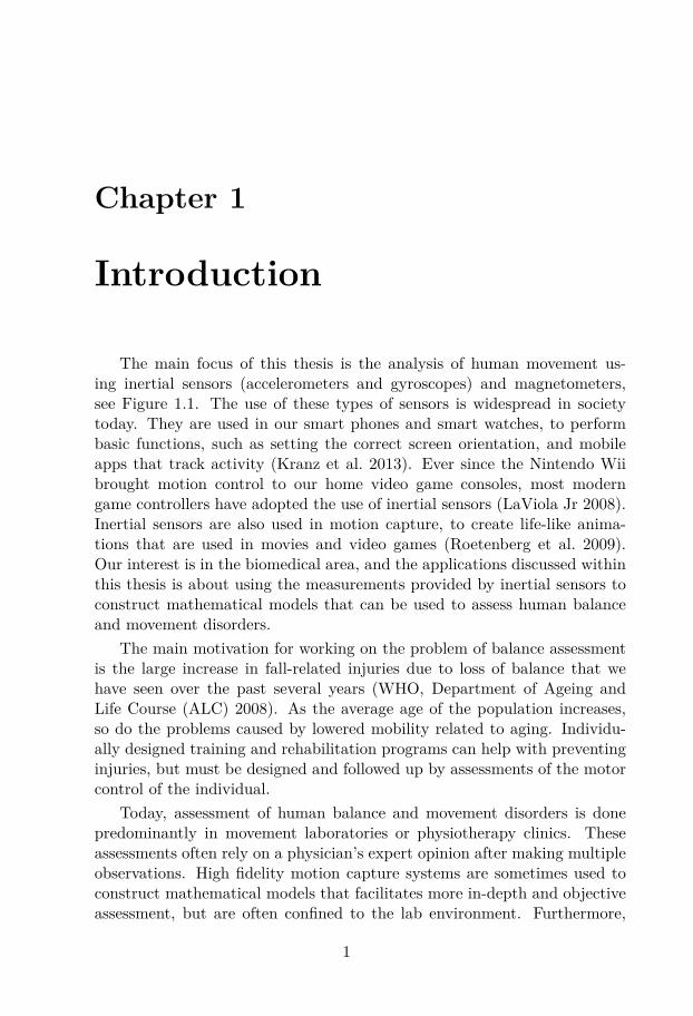
The main focus of this thesis is the analysis of human movement us-ing inertial sensors (accelerometers and gyroscopes) and magnetometers,see Figure 1.1. The use of these types of sensors is widespread in societytoday. They are used in our smart phones and smart watches, to performbasic functions, such as setting the correct screen orientation, and mobileapps that track activity (Kranz et al. 2013). Ever since the Nintendo Wiibrought motion control to our home video game consoles, most moderngame controllers have adopted the use of inertial sensors (LaViola Jr 2008).Inertial sensors are also used in motion capture, to create life-like anima-tions that are used in movies and video games (Roetenberg et al. 2009).Our interest is in the biomedical area, and the applications discussed withinthis thesis is about using the measurements provided by inertial sensors toconstruct mathematical models that can be used to assess human balanceand movement disorders.
The main motivation for working on the problem of balance assessmentis the large increase in fall-related injuries due to loss of balance that wehave seen over the past several years (WHO, Department of Ageing andLife Course (ALC) 2008). As the average age of the population increases,so do the problems caused by lowered mobility related to aging. Individu-ally designed training and rehabilitation programs can help with preventinginjuries, but must be designed and followed up by assessments of the motorcontrol of the individual.
Today, assessment of human balance and movement disorders is donepredominantly in movement laboratories or physiotherapy clinics. Theseassessments often rely on a physician’s expert opinion after making multipleobservations. High fidelity motion capture systems are sometimes used toconstruct mathematical models that facilitates more in-depth and objectiveassessment, but are often confined to the lab environment. Furthermore,
1

2 1.1. Inertial sensors
Figure 1.1: Two sensor platforms which contain inertial and magneticsensors. The Xsens MTw Awinda wireless motion tracker (left) and a mod-ern smart phone (right).
this type of assessment is expensive since it uses work hours of the physicianand the limited lab resources. The same reasons lead to another problem,that assessment is performed infrequently and is therefore vulnerable toshort-term fluctuations.
Inertial sensors has the potential to solve both of these issues due to theirrelatively low cost and small size. Allowing the assessment to be performedoutside of the lab, preferably even in the patient’s home, would ease theworkload of the physicians and use less lab resources. The sensors may beworn throughout the daily life of the patient, which allows for more frequentassessment. We are specifically interested in using as few sensors as possible,to obtain an assessment technique that is unobtrusive and easy to maintain.
1.1 Inertial sensors
Throughout this thesis, the term inertial sensors will be used to denoteboth three-axis accelerometers and three-axis gyroscopes. Accelerometersmeasure the linear acceleration of the sensor, which includes the gravita-tional acceleration component, g ∈ R3, in addition to the acceleration caused

Chapter 1. Introduction 3
Global frame
Sensor frame
Figure 1.2: A global Earth-fixed reference frame and a sensor-fixed referenceframe. The rotation from the global frame to the sensor frame defines theorientation of the sensor.
by the movement of the sensor itself. The gravitational acceleration variesdepending on where on Earth you are. Specifically, how close the poles andhow far above the center of the earth you are, as well as the density of thebedrock beneath your feet, will have an effect on the magnitude of g, whichis measured in the Euclidean norm, ‖g‖2. For instance, in Smygehuk (south-ernmost point in Sweden) ‖g‖2 = 9.815220m s−2 has been measured, whichis slightly lower than at Treriksröset (northernmost point in Sweden), where‖g‖2 = 9.823944m s−2 has been measured (Lantmäteriet 2018). Typically,‖g‖2 is approximated to be constant in the vicinity of a specific location,and this constant value can be used to calibrate the sensor.
Gyroscopes measure angular velocity, the rate of change of the sensor’sorientation. The sensor’s orientation is typically defined as the rotationbetween two Cartesian reference frames, the (global) navigation frame andthe sensor frame, see Figure 1.2. In most applications we are interestedin how the sensor moves in the navigation frame, and therefore we needto know its orientation. Integrating the gyroscope signal is a method forobtaining an estimate of the sensor’s orientation relative to its initial ori-entation. However, as the measurements are typically biased and noisy, theintegration will cause the estimates to drift and become more erroneous withtime. This phenomenon will be referred to as integration drift.
Luckily, we can often use information from other sensors to obtain ab-solute observations of the orientation. This additional information can beused to correct for the integration drift of the gyroscope. Combining theinformation from multiple different sensors like this is referred to as sensorfusion (Gustafsson 2010). The g vector is typically aligned with the ver-

4 1.2. Magnetometers
tical direction in the navigation frame, pointing radially outwards from thecenter of the Earth. Therefore, an accelerometer that is stationary in thenavigation frame can be used to estimate the inclination of the sensor, whichis the angle between the vertical direction in the navigation frame and theaxis that has been defined as the vertical in the sensor frame. Note that theinclination provides no information about the heading, which is defined asthe rotation angle around the vertical in the navigation frame. Therefore,inertial sensors alone can provide accurate estimates of the inclination butwill yield erroneous estimates of the heading due to the integration drift.
Today, inertial sensors see abundant use and play an important rolein navigation (Woodman 2007), motion capture (Hol 2011; Kok 2016) andhealthcare and sports monitoring (Avci et al. 2010).
1.2 Magnetometers
Magnetometers are sensors that measure the local magnetic field, andare also frequently used in sensor platforms together with inertial sensors.Their most common use is similar to that of a regular compass; to providean absolute observation of the heading. In the most commonly used refer-ence frames in navigation, the horizontal axes will point in the longitudinaland latitudinal directions. In such a reference frame, the horizontal com-ponents of the Earth magnetic field will point to the magnetic north poleand a heading of 0◦ typically aligns with this direction. However, magneto-meters used for this purpose are also susceptible to magnetic disturbancesand will function poorly when they are surrounded by metallic or electric-ally conducting objects that have their own magnetic fields superimposedto the Earth magnetic field. This is important to be aware of when usingmagnetometer measurements to observe the heading. Having a prior modelof the local Earth magnetic field can help to decide which measurementsthat may be affected by magnetic disturbances. In other applications, localfluctuations in the magnetic field can be exploited for benefit instead. It ispossible to construct a map of the magnetic environment in buildings forexample, which can be used in e.g. indoor navigation (Kok et al. 2013; Solinet al. 2015).
1.3 Outline of introductory chapters
The introductory chapters of this thesis consists of Chapter 1–4, and willserve to provide background and context to Paper I–IV, that make up thelatter part of the thesis. Chapter 2 introduces biomechanical models thatwe use to describe the dynamics of a standing human. In the same chapter

Chapter 1. Introduction 5
we also introduce some of the most common mathematical models usedto describe the mechanisms behind human balance. Chapter 3 introducesthe various estimation problems that we face when working with inertialsensors. Measurement models for the inertial and magnetic sensors are in-troduced, as are the estimation problems related to orientation estimation,calibration of the sensors, calibration of the biomechanical model and identi-fication of neuromuscular control. The methods that are used to solve thesevarious problems are presented in the context of the problems themselves,rather than a standalone method summary, to emphasize the applicationsconsidered in this thesis. Finally, Chapter 4 concludes by summarizing thecontributions of this thesis and potential future work is discussed.
1.4 Summary and contributions of the papers
The four papers contain the main contributions of this thesis. The focusof these papers concerns the practical use of inertial and magnetic sensorsfor analyzing human movement. Each paper contains examples where datafrom real sensors are used to illustrate the functionality of the proposedmethods. Here follows a short summary of the papers.
1.4.1 Paper I
In this paper we propose a practical calibration method for acceleromet-ers. The method only requires a gyroscope as additional equipment, whichis commonly included in inertial sensor platforms. Lower quality accelero-meters often have significant errors that have to be compensated for, suchas misaligned sensor axes, varying gains and biases. Through sensor fusionof the accelerometer and the gyroscope we estimate the orientation of thesensor platform. By observing the accelerometer measurements for differ-ent orientations, we are able to identify a set of model parameters that canbe applied to the raw accelerometer measurements to compensate for thesetypes of errors.
1.4.2 Paper II
Here we consider a different type of calibration problem, which is toidentify the position of a joint in a biomechanical model, with respect totwo inertial sensors attached to the two segments adjacent to the joint.This can be thought of as calibrating the biomechanical model. The prob-lem is formulated as an optimization problem, to find the joint positionsthat minimize a cost function, that is based on the kinematic constraints

6 1.4. Summary and contributions of the papers
of the biomechanical model. The contribution of this paper is the experi-mental evaluation and minor extension of three methods designed to solvethis problem, where each method uses a differently formulated cost function.The evaluation is based on real data from sensors attached to two rigid cyl-indrical segments joined together by a spherical joint, where the true jointcenter with respect to the sensors could be measured.
1.4.3 Paper III
This paper concerns identification of the dynamics in unknown feedbackcontrollers that operate in closed loop systems. The human balance systemcan be seen as one such closed loop system, where the controller consists ofthe central nervous system (CNS), which senses the state of the body andactivates muscles to prevent us from falling. A recently proposed nonlinearsystem identification method (Mattsson et al. 2018) is applied to identify twodifferent types of controllers; a simulated neuromuscular controller balancinga standing human and a real-world controller for a position servo that uses aDC-motor. Simulated and real inertial sensor data is used for identification.Thus, the contribution of this paper is not the identification method itselfbut rather it’s application to closed loop identification and making use ofinertial sensor data to do so.
1.4.4 Paper IV
In this paper we make use of inertial and magnetic sensor measurementsfrom a smart phone to quantify the severity of hand tremor, which is amovement disorder and a primary symptom of neurological disorders suchas Parkinson’s disease (PD) and Essential tremor (ET). The contributionof this paper is the full description of a proposed method for tremor quan-tification. A tremor signal is obtained from smart phone measurements,which considers the involuntary movement caused by tremor as the devi-ation in position from an estimated voluntary movement. The amplitudesof this tremor signal is then modeled as a stochastic process in the formof a Markov chain. An invariant distribution is extracted from the Markovchain, which can then be interpreted as a probability distribution of thetremor severity. The method is then illustrated on real data from a PD pa-tient with deep brain stimulation (DBS) implanted, which is a therapy usedto treat the symptoms, such as tremor, of PD. Using the proposed methodit is possible to distinguish between different DBS settings, which indicatesthat it could be used for therapy individualization.

Chapter 2
Biomechanical modeling andcontrol
In this chapter we derive biomechanical models that can be used toanalyze the balance mechanisms in standing humans. A very general modelof the musculoskeletal system in humans is a kinematic chain, where eachbody segment is approximated as a rigid body link, which are connectedby joints that constrain the relative movement of all links. The degrees offreedom in such a model is 6n−m, where n is the number of individual linksand m is the number of constraint equations due to the joints.
When studying standing human balance however, it is common to ap-proximate the musculoskeletal system using a much simpler model, the in-verted pendulum. Numerous studies have used this model to study standinghuman balance (Gage et al. 2004; Winter 1995). The motivation for thisapproximation is that there are two main strategies that humans use tomaintain upright standing; the ankle strategy and the hip strategy. Thesestrategies essentially mean that the central nervous system activates muscles,which generates torques around the ankle joint and the hip joint, respect-ively, hence the names. The inverted single pendulum, is a kinematic chainwith one joint, the ankle joint, and all body segments above the feet arelumped together as one link. By adding one joint we get the inverted doublependulum, where the added joint represent the hip joint, the lower linkrepresent the legs and the upper link represent the head, arms and trunksegments.
By only considering one or two links, we have reduced the degrees offreedom considerably, compared to a complete kinematic chain model withall body segments modeled by separate links. We can reduce the degreesof freedom further by constraining the movement of the inverted pendulumto a plane. This movement constraint is motivated by the fact that, given
7

8 2.1. Lagrangian formalism
a sufficient stance width, a standing human moves predominantly in theanterior-posterior directions. This results in only one rotation angle for eachjoint instead of three. Finally, if we fix the location of the feet, the anklejoint becomes stationary, and the position of the center of mass (CoM) ofeach link can be determined by only knowing the joint angles. Thus, thedegrees of freedom of the model are reduced to one for the planar invertedsingle pendulum and two for the planar inverted double pendulum.
2.1 Lagrangian formalism
We will make use of the Lagrangian formalism to derive the equations ofmotion (EoM) that describe the rigid body dynamics of the biomechanicalmodels. First we form the Lagrangian
L(q, q) = Ek(q, q)− Ep(q), (2.1)
where Ek(q, q) is the kinetic energy and Ep(q) is the potential energy of thesystem. The Lagrangian depends on the generalized coordinates q ∈ Rn andtheir time derivatives (generalized velocities) q = dq
dt , where n is the numberof degrees of freedom of the system. For each generalized coordinate we getone EoM, which is computed as
d
dt
∂L
∂qi− ∂L
∂qi= 0, i = 1, . . . , n. (2.2)
For the case of the inverted pendulum the generalized coordinates will bethe angles φ between each link and the global vertical direction and thegeneralized velocities will be the angular velocities φ.
2.2 Inverted single pendulum
Starting with the simplest case, the inverted single pendulum, we firstnote that the Cartesian coordinates (x, y), of the CoM are uniquely determ-ined by the joint angle φ
x = c sinφ (2.3)y = c cosφ, (2.4)
where c is the distance from the joint to the CoM. The Lagrangian is
L = mv2
2 + I φ2
2 −mgy, (2.5)

Chapter 2. Biomechanical modeling and control 9
where m is the mass of the link, v is the linear velocity of the CoM, I isthe moment of inertia w.r.t. the rotation axis and g is the gravitationalacceleration. Using (2.3)-(2.4) we can express the Lagrangian in terms of φand φ
L = m
2 (x2 + y2) + I φ2
2 −mgy
= mc2 φ2
2 (cos2 φ+ sin2 φ) + I φ2
2 −mgc cosφ
= mc2 + I
2 φ2−mgc cosφ. (2.6)
Using (2.2) we find that the EoM is
(mc2 + I) φ−mgc sinφ = 0, (2.7)
which is also straightforward to derive using Newton’s second law.
2.3 Inverted double pendulumIn an inverted double pendulum, see Figure 2.1, the CoM coordinates
for each separate link is given by
x1 = c1 sinφ1 (2.8)y1 = c1 cosφ1 (2.9)x2 = l1 sinφ1 + c2 sinφ2 (2.10)y2 = l1 cosφ1 + c2 cosφ2, (2.11)
where l is the length of the link and subscripts now indicate which link acertain quantity belong to. The Lagrangian then becomes
L = m1v21
2 + m2v22
2 + I1 φ21
2 + I2 φ22
2 −m1gy1 −m2gy2
= m12 (x2
1 + y21) + m2
2 (x22 + y2
2) + I1 φ21
2 + I2 φ22
2 −m1gy1 −m2gy2
= m1c21 φ
21
2 (cos2 φ1 + sin2 φ1) + m22 (l21 φ
21 cos2 φ1 + c2
2 φ22 cos2 φ2
+ 2l1c2 φ1 φ2 cosφ1 cosφ2 + l21 φ21 sin2 φ1 + c2
2 φ22 sin2 φ2
+ 2l1c2 φ1 φ2 sinφ1 sinφ2) + I1 φ21
2 + I2 φ22
2 −m1gy1 −m2gy2
= m12 c2
1 φ21 +m2
2 (l21 φ21 +c2
2 φ22 +2l1c2 φ1 φ2 cos(φ1 − φ2))

10 2.3. Inverted double pendulum
φ1
φ2
m1g
m2g
c1
c2
l1
x
y
Figure 2.1: The inverted double pendulum model.
+ I1 φ21
2 + I2 φ22
2 −m1gc1 cosφ1 −m2g(l1 cosφ1 + c2 cosφ2),(2.12)
and the two equations of motion are then given by
m1c21 φ1 +m2
(l21 φ1 +l1c2 φ2 cos(φ1 − φ2) + l1c2 φ
22 sin(φ1 − φ2)
)
+ I1 φ1−m1gc1 sinφ1 −m2gl1 sinφ1 = 0,(2.13)

Chapter 2. Biomechanical modeling and control 11
and
m2(c2
2 φ2 +l1c2 φ1 cos(φ1 − φ2)− l1c2 φ21 sin(φ1 − φ2)
)
+ I2 φ2−m2gc2 sinφ2 = 0.(2.14)
For systems with multiple degrees of freedom it is often convenient to expressthe EoM on the form
M(φ) φ+C(φ, φ) φ+G(φ) = 0, (2.15)
where we see that inserting (2.13)-(2.14) yields[m1c2
1 +m2l21 + I1 m2l1c2 cos(φ1 − φ2)m2l1c2 cos(φ1 − φ2) m2c2
2 + I2
]
︸ ︷︷ ︸=M(φ)
[φ1φ2
]
+[
0 m2l1c2 φ2 sin(φ1 − φ2)−m2l1c2 φ1 sin(φ1 − φ2) 0
]
︸ ︷︷ ︸=C(φ,φ)
[φ1φ2
]
+[−m1gc1 sinφ1 −m2gl1 sinφ1
−m2gc2 sinφ2
]
︸ ︷︷ ︸=G(φ)
= 0.
(2.16)
2.4 Neuromuscular control
So far, the EoM that we have derived for inverted single and doublependula only contain the forces of gravity. Inverted pendula are inherentlyunstable; for any deviation from the vertical equilibrium point φ = 0, thependulum will start to fall. Humans are similar, without the aid of ourmuscles to counter the force of gravity we would meet the same fate. Whenthe muscles that connect to the joint tendons contract, the result can be seenas a torque that is generated and acts on the adjacent body segments. Thistorque will be referred to as the joint torque. The human musculoskeletalsystem is inherently redundant in the sense that multiple muscles act acrosseach joint. We view a joint torque as the net torque from all contributingmuscles.
The muscle activity is controlled by the CNS, which sends activation sig-nals out to the muscles. To choose appropriate activation signals, the CNSreceives information, y, from biological sensors in our body and chooses anappropriate response depending on which task that should be performed.This is similar to how controllers work in a feedback loop. The task can

12 2.4. Neuromuscular control
be seen as a certain desired configuration or state of the body segments,and is the equivalent of a reference signal, r. The reference signal is com-pared to the information about the current state and the control actionthat is generated by the CNS are the joint torques that should move thebody segments closer to the desired state. Therefore, a control mechanismin the CNS that takes information from our biological sensors as input andoutputs a joint torque by activating muscles will be referred to as a neur-omuscular controller. As φ = φ = 0 corresponds to upright standing in ourbiomechanical model, the reference signal in that case will correspond tothis equilibrium point. Figure 2.2 shows a block diagram, which illustratesthe closed neuromuscular control loop.
Neuromuscularcontroller
Musculoskeletalsystem (plant)
d
Tr
Biologicalsensors φ
y
Figure 2.2: A closed neuromuscular control loop in humans.
We can expand the EoM to include the joint torques, T , as
M(φ) φ+C(φ, φ) φ+G(φ) = DT, (2.17)
where D is a matrix with elements Dij = ±1, that describes how the jointtorques affect the segments or Dij = 0 if a joint torque does not affect somesegments at all. For the inverted single pendulum we simply have D = 1and in the inverted double pendulum we have
D =[1 −10 1
], (2.18)
which follows from Newton’s third law of equal and opposite forces.Apart from the forces of gravity and the joint torques generated by
the neuromuscular controller, the plant may also be affected by externaldisturbances, denoted by d in Figure 2.2. External disturbances play animportant role in the identification of the neuromuscular controller, whichis introduced in Chapter 3 and is the main topic of Paper III. The externaldisturbances can be designed as an exogenous input signal to the closedneuromuscular control loop, which allows information about the controllerto be extracted via observations of the movement of the human.

Chapter 2. Biomechanical modeling and control 13
2.4.1 State-space representation and linearization
We can formulate the extended EoM in (2.17) as a nonlinear state-spacemodel
[φ
φ
]=[0 I
0 −M(φ)−1C(φ, φ)
] [φ
φ
]
+[
0−M(φ)−1G(φ)
]+[
0M(φ)−1D
]T
, (2.19)
which is a system of nonlinear ordinary differential equations (ODE), wherex =
[φ φ
]>is referred to as the state.
It is often convenient to approximate (2.19) as a linear state-space model,since control theory for linear systems is simpler and there exists manypowerful mathematical methods for analysis or controller design (Kailath1980; Rugh 1996). The EoM (2.17) can be expressed as the nonlinear func-tion
f(φ, φ, φ, T ) = M(φ) φ+C(φ, φ) φ+G(φ)−DT = 0. (2.20)
Let the variables be denoted by z =[φ φ φ T
]>. We then select a
linearization point z0 =[φ0 φ0 φ0 T0
]>and use a first-order Taylor
expansion to approximate f as
f(φ, φ, φ, T ) = ∂f
∂φ
∣∣∣z=z0
(φ− φ0) + ∂f
∂ φ
∣∣∣z=z0
(φ− φ0)
+ ∂f
∂ φ
∣∣∣z=z0
(φ− φ0) + ∂f
∂T
∣∣∣z=z0
(T − T0)(2.21)
= fφ0∆φ + fφ0∆φ + fφ0
∆φ + fT∆T , (2.22)
where
fq0 = ∂f
∂q
∣∣∣z=z0
, ∆q = q − q0, q = {φ, φ, φ, T}. (2.23)
Note that the Taylor expansion (2.21) does not require the function valueat the equilibrium point, since f(z0) = 0, ∀z0, per definition. Then we haveobtained a linear state-space model for
[∆φ ∆φ
]>according to
[∆φ
∆φ
]=[
0 I
−f−1φ0fφ0 −f−1
φ0fφ0
] [∆φ
∆φ
]+[
0−f−1
φ0fT
]∆T . (2.24)

14 2.4. Neuromuscular control
We now choose to linearize around the equilibrium point z0 = 0, to obtaina state-space model on the form
x = Ax+BT, (2.25)
where
A =[
0 I
−f−1φ0fφ0 −f−1
φ0fφ0
], B =
[0
−f−1φ0fT
](2.26)
fφ0= M(φ0) (2.27)
fφ0= ∂
∂ φ
(C(φ0, φ) φ
)∣∣∣φ=φ0
(2.28)
fφ0 = ∂
∂φ
(M(φ) φ0 +C(φ, φ0) φ0 +G(φ)
)∣∣∣φ=φ0
(2.29)
fT = −D. (2.30)
The linearized state-space representation of the EoM is a good approxima-tion for sufficiently small deviations from the equilibrium point.
2.4.2 Modeling the neuromuscular control law
The neuromuscular controller is what we are primarily interested in mod-eling. A good model should not only be able to predict the response of thetrue controller, but also be easy to interpret so that it can provide meaning-ful insight about individual performance. Unlike the biomechanical modelof the musculoskeletal system, there are no well defined laws of physics thatcan completely describe the dynamics of the neuromuscular controller. Evenif we are able to describe the function of groups of several neurons we arestill far from understanding the extremely complex and interconnected net-work, consisting of close to 100 billion neurons, which is the human brain(Herculano-Houzel 2009). However, many researchers have studied the neur-omuscular control in human balance and have proposed different types ofmodels as well as methods to identify these from empirical data. These aredynamical models that aim to describe the relationship between the inputsand outputs of the neuromuscular controller, which is significantly moresimple than trying to explain the function of the brain itself. In this section,we will give a very brief introduction to some of the most common modelsthat have been proposed.
In the most general sense, the neuromuscular control law can be formu-lated as
T (t) = h(y(τ), r(τ), τ, θ(τ)), −∞ < τ ≤ t, (2.31)

Chapter 2. Biomechanical modeling and control 15
where we state that the joint torque T is a function of the sensory inform-ation y and the reference signal r. The function h(·) can be any nonlinearfunction, and may be parametrized by possibly a limitless number of para-meters, denoted by θ, which may also be time-varying. The control law isnon-static, and could in general depend on the infinite history of its argu-ments up to time t, denoted by −∞ < τ ≤ t. A general model like this isnot specific enough to be of practical value, and the measurements availableto us also place restrictions on how accurately we can actually describe thecausal relationship in (2.31). Therefore, we assume certain model structuresfor the function h(·) and the parameters θ(t). A common assumption is thatthe neuromuscular controller is linear and time-invariant (LTI) and that thereference signal is constant, corresponding to the desired equilibrium point(Park et al. 2004; Peterka 2002). These assumptions reduces (2.31) to
T (t) =∫ ∞
0h(t, θ)y(t− τ)dτ, (2.32)
where h(t, θ) is a function of time, also known as the impulse response ofthe controller, which depends on a finite set of constant parameters θ. Anequivalent formulation of (2.32) in the frequency domain is
T (s) = H(s, θ)y(s), (2.33)
where H(s, θ) is the transfer function of the controller for the Laplace vari-able s, and T (s) and y(s) are the Laplace transforms of the time-domainsignals T (t) and y(t), respectively. Below we describe controllers that as-sume the LTI form in (2.32).
Proportional derivative (PD) controller
One of the simplest controllers that one can think of is a proportionalderivative (PD) controller. The output of the controller is then chosen as alinear combination of the observed joint angle and its first time derivative
T (t) =[Kp Dp
] [φ(t)φ(t)
]= Tp(t), (2.34)
where the model parameters correspond to θ = {Kp, Dp}. The type offeedback that Tp(t) represents is often referred to as passive or intrinsicfeedback as it can be thought of as describing the passive dynamics of themuscles, tendons and soft tissue, which gives the standing human propertiessimilar to that of a damped spring (Winter et al. 1998). The parameters Kp
and Dp correspond to the stiffness and damping coefficients. While a PDcontroller certainly can be used in practice to stabilize inverted single anddouble pendulua it is not a very realistic model of neuromuscular control,as it does not take muscle activation and neural time delay into account.

16 2.4. Neuromuscular control
Time delayed PD controller
A natural extension of the PD controller in (2.34) is to add feedbackfrom time delayed states, which takes into account the time it takes forneuronal signals to travel from the biological sensors to the CNS and backto the muscles (Peterka 2002). This extended model can be formulized as
T (t) =[Kp Dp Ka Da
]
φ(t)φ(t)
φ(t− τ)φ(t− τ)
= Tp(t) + Ta(t), (2.35)
where the model parameters now correspond to θ = {Kp, Dp,Ka, Da, τ} andτ is the neural time-delay. Note that in a biomechanical model with multiplejoints, different delays will be used for every joint since they involve differentmuscle groups and neural pathways. The term Ta(t), which has been addedto (2.34) to create (2.35), is often referred to as active or reflexive feedbackas it takes into account the delays in neuronal signals that activates specificmuscle groups.
In some cases the muscle activation dynamics are also described, whichcan be modeled in the frequency domain as
Ta(s) = (Kaφ(s) +Dasφ(s))e−τsHact(s), (2.36)
where Hact(s) is the transfer function that models the muscle activationdynamics. In Boonstra et al. (2013) and Engelhart et al. (2016), Hact(s) ismodeled as a second-order system
Hact(s) = ω20
s2 + 2ζω0s+ ω20, (2.37)
where ω0 is the natural frequency and ζ is the damping of the muscle ac-tivation dynamics, both of which are then included in the set of modelparameters θ. This type of model has been used frequently to simulate amore realistic neuromuscular controller. We also utilize a similar simulationmodel in Paper III.
Linear quadratic (LQ) controller
Another way to view neuromuscular control is that the CNS in someway generates controller outputs which minimize an internal cost function,which is known as optimal control see Kuo (1995). A special case is the linearquadratic (LQ) controller, where the cost function is quadratic, which is the

Chapter 2. Biomechanical modeling and control 17
optimal controller for LTI plant models such as (2.25). The LQ controllerfinds the control law such that the cost function
J =∫ ([
φ>(t) φ>(t)
]Q
[φ(t)φ(t)
]+ T>(t)RT (t)
)dt, (2.38)
is minimized, where Q and R are positive semi-definite matrices that de-termine how much weight the states and the controller output are given,respectively. The proportions of Q relative to R will determine the con-troller properties and therefore, these are the model parameters for the LQcontroller i.e. θ = {Q,R}. For LTI systems (2.38) has a closed form solution,which yields a control law on the form
T (t) = H
[φ(t)φ(t)
](2.39)
H = −R−1B>P, (2.40)
where P is found by solving the continuous time algebraic Riccati equation
A>P + PA− PBR−1B>P +Q = 0, (2.41)
and A and B come from the linearized plant model (2.25).
Frequency response function (FRF)
It is also possible to characterize the neuromuscular controller in thefrequency domain as
T (iω) = H(iω)φ(iω), (2.42)
for the angular frequency ω. The frequency response function (FRF) of thecontroller H(iω) is a complex-valued function that can be described on polarform by its magnitude and phase
H(iω) = |H(iω)|eiArgH(iω). (2.43)
The FRF is often considered a non-parametric model since it cannot be de-scribed by a finite set of parameters θ, unlike the the previous (parametric)controller models we have studied. A rational transfer function model de-scribed by a finite set of parameters may be used to approximate the FRF,in which case the parameters are estimated to fit the empirical FRF. Toconstruct an FRF model for the neuromuscular controller, one makes use ofthe LTI assumption and a known external disturbance signal d, which hasbeen designed specifically to excite the system at certain frequencies. In this

18 2.4. Neuromuscular control
case, the LTI assumption implies that if d has a periodic component for theangular frequency ω0, the output of the neuromuscular controller will alsohave periodic components at ω0, but with a different amplitude and phase.Designing the external disturbance d is therefore important, as it decidesat which frequencies it is possible to determine the FRF. In theory a whitenoise signal can be used as it contains all frequencies, but in practice thefrequency band will be limited by the experimental setup.
The FRF models can be constructed by opening the closed control loopseen in Figure 2.2,
H(iω) = −HdT (iω)H−1dφ (iω), (2.44)
where HdT (iω) and Hdφ(iω) are the cross-spectral density (Stoica, Moses etal. 2005) matrices for the external disturbance d and the controller output Tand the plant output φ, respectively. This is known as the joint input-outputmethod (Kooij et al. 2005; Ljung 1999).
Nonlinear controllers
Thus far we have only considered models of the neuromuscular controllerthat rely on the LTI assumption. In reality however, the neuromuscularcontroller contains nonlinearities and expresses a time-varying behaviour.Therefore, we would like to find more flexible model structures that candescribe these properties. However, a more flexible model structure generallymeans that the number of model parameters increases, which makes it harderto find good parameter values. Flexible nonlinear models can also be harderto interpret compared to e.g. the simple PD controller, where the parameterscan be interpreted as the stiffness and damping coefficients in an oscillator.In Paper III we consider a flexible model structure for the controller, whichcombines a nominal linear model with an overparametrized error model todescribe the nonlinearities according to
T (t) = Θϕ(t) + Zγ(t). (2.45)
The linear model is described by Θϕ(t), where ϕ(t) ∈ Rnϕ×1 is a vectorcontaining the controller inputs and Θ ∈ RnT×nϕ is a matrix that containsthe linear parameters. Similarly the nonlinear model is described by Zγ(t),but here γ(t) ∈ Rnγ×1 is a vector containing a set of nonlinear basis functionsapplied to the controller inputs and Z ∈ RnT×nγ is a matrix containing thenonlinear parameters. The nonlinear parameters are the coefficients whichare multiplied with nonlinear basis functions of the information given asinput to the controller. The number of controller outputs, nT , is determinedby the biomechanical model, while the dimensions of the parameter matrices,

Chapter 2. Biomechanical modeling and control 19
nφ and nγ , are determined by the model structure, the assumptions aboutϕ(t) and γ(t). To try to minimize the model complexity, the model canbe constructed using a sparse set of nonlinear parameters, such that thenominal linear model describes as much of the dynamics as possible anda minimum number of nonlinear basis functions are used (Mattsson et al.2018).
2.4.3 Modeling the biological sensors
The biological sensors that contribute with information to the CNS inhuman balance are primarily the visual, vestibular and proprioceptive sens-ory systems. We have used y(t) to denote the information that is received bythe CNS, and for the previously discussed controller models, we have onlyassumed that y(t) consists of the plant outputs φ(t), φ(t) and possibly timedelayed versions of these signals. A more realistic model should include anoise term, since the information that the CNS receives about the currentstate of the plant is not accurate. The inaccuracies in the sensory informa-tion can be seen as a natural cause of the involuntary body sway that canbe observed in quiet (meaning unperturbed) upright standing.
A model that has been widely used is the sensory weighting model(Peterka 2002; Peterka and Loughlin 2004)
y(t) =[wvis wves wpro
]yvis(t)yves(t)ypro(t)
, (2.46)
where wvis, wves and wpro are weights and yvis(t), yves(t) and ypro(t) representthe information from the visual, vestibular and proproiceptive sensors, re-spectively. Evidence from previous studies (Mahboobin et al. 2005; Peterkaand Loughlin 2004) suggests that humans use an adaptive sensory reweight-ing scheme to modulate the information used by the neuromuscular control-ler. This means that the weights adapt to physiological or environmentalconditions. For example, closing your eyes will remove the visual informa-tion, so other sensory systems have to compensate.


Chapter 3
Estimation techniques usinginertial sensors
Regardless if we want to learn something about an unknown quantityor describe physical phenomena, we compute estimates based on what weobserve. In this thesis, the observations are measurements from inertial andmagnetic sensors. Here, we provide a suitable background to the variousestimation problems that arise in the papers.
3.1 Sensor models
The inertial and magnetic sensors that we make use of are microelec-tromechanical systems (MEMS), embedded in microchips that are solderedto a circuit board, forming a sensor platform. Each sensor has three indi-vidual, orthogonal sensor axes, so all measurements are in 3D. The meas-urements of linear acceleration, angular velocity and the local magnetic fieldare all with respect to a reference frame, fixed in the sensor platform. Werefer to this reference frame as the sensor frame (S), and it is defined tobe fixed with its axes and origin aligned with the accelerometer axes andorigin.
In many applications we are interested in relating the measured quantit-ies to a global Earth-fixed reference frame, often referred to as the navigationor global frame (G). On Earth it is logical for the vertical axis in the globalframe to be chosen to be parallel to the gravitational acceleration vector,which points toward the center of the Earth. The horizontal axes are oftenchosen differently depending on the situation. In navigation situations (e.g.aviation), the two horizontal axes typically point to the north, or latitudinaldirection, and the east, or longitudinal direction. However, when analyzinghuman movement it often makes more sense to define the horizontal axes to
21

22 3.1. Sensor models
z
x
y
S–frame
x
y
z
G–frame
Figure 3.1: An illustration of the difference between the sensor frame (S),which has its axes fixed with respect to the sensor platform and the globalframe (G), which has its axes fixed with respect to Earth.
suit the experimental setup. For example, when studying human balance,the human subject is often facing the same direction during a movementtask. Then it is reasonable to have one axis pointing forward in the anteri-or/posterior direction and one axis pointing sideways in the medial/lateraldirection. Figure 3.1 illustrates the difference between the S–frame and theG–frame.
3.1.1 Orientation representations
To transform the measured quantities from one reference frame to an-other is simply a change of orthonormal basis vectors in R3. We make use ofrotation matrices, which are part of the special orthogonal group R ∈ SO(3).For example if vG is a vector in the global frame and vS is the same vector,but expressed in the sensor frame, then we have that
vS = RS GvG, (3.1)
where RS G is the rotation matrix that when multiplied with any vector inthe G–frame, maps that vector into the S–frame. The inverse rotation is the

Chapter 3. Estimation techniques using inertial sensors 23
x y
z
xy
z
x y
z
φx
φy
φz
φx
φy
φz
Figure 3.2: From left to right; rotations around the z–, y– and x–axes usingthe corresponding Euler angles φz, φy and φx.
opposite, i.e.(RS G
)−1=(RS G
)>= RG S. The columns of the rotation
matrix RG S give the coordinates of the three unit vector axes of the S–frame expressed in the G–frame. Therefore, a rotation matrix representsthe relative orientation of one reference frame with respect to another.
A rotation can be represented in a number of ways. The rotation matrixis a non-minimal representation of a rotation. It has 9 elements, but each rowand column is a unit vector, which gives 6 constraints. Hence a rotation canbe described by 3 free variables. One possible parametrization uses Eulerangles. If a reference frame is defined by the orthonormal basis vectors[x y z
]where x, y, z ∈ R3, the Euler angles φ =
[φx φy φz
]>represent
rotation angles around the x, y, z axes as indicated by the subscripts. Theangles φx, φy and φz are commonly referred to as the roll, pitch and yawangles, respectively. The complete rotation matrix can be constructed froma sequence of rotations around each individual axis, for example
R =
1 0 00 cosφx − sinφx0 sinφx cosφx
cosφy 0 sinφy0 1 0
− sinφy 0 cosφy
cosφz − sinφz 0sinφz cosφz 0
0 0 1
= RxRyRz
,
(3.2)
which represents a z–y–x rotation sequence. The rotations that correspondto Rz, Ry and Rx are shown in Figure 3.2. Note that the sequence ofrotations is important; even if the Euler angles are the same, a differentrotation sequence will generally yield a different rotation matrix. Anotherway to represent rotations is using unit quaternions, q, which are unit vectorsin R4. A unit quaternion that represent the same rotation as in (3.2) can

24 3.1. Sensor models
be constructed from the same Euler angles
q =
cos φx2sin φx
200
�
cos φy20
sin φy2
0
�
cos φz200
sin φz2
= qx � qy � qz
, (3.3)
where � represents the quaternion product, which is a special algebraicoperation for quaternions. More about quaternion algebra can be found ine.g. Särkkä (2007). Just like (3.2), we have that (3.3) represents the z–y–x rotation sequence, and changing the order of quaternion multiplicationschanges the rotation sequence accordingly. Unit quaternions can also beused to parametrize rotation matrices
R(q) =
2q21 + 2q2
2 − 1 2(q2q3 − q1q4) 2(q2q4 + q1q3)2(q2q3 + q1q4) 2q2
1 + 2q23 − 1 2(q3q4 − q1q2)
2(q2q4 − q1q3) 2(q3q4 + q1q2) 2q21 + 2q2
4 − 1
(3.4)
q =[q1 q2 q3 q4
]>, (3.5)
and provided that q represents the same rotation sequence as in (3.2), wehave that (3.4) will produce the exact same rotation matrix.
3.1.2 Measurement models
In this section we introduce the models that are used to describe themeasurements obtained from inertial sensors and magnetometers. Since thesensors are sampled in discrete time we will let, t = 1, 2, . . . , denote a discretetime index. The rotation matrix RS G(t) describes the relative orientation ofthe sensor frame with respect to the global frame. Furthermore, these mod-els assume that the sensors are calibrated. Sensor calibration is discussedfurther in section 3.3 and is the main topic of Paper I.
Accelerometer
Accelerometer measurements are modelled as
ySa(t) = RS G(t)(aG(t) + gG) + ea,t, (3.6)
where aG(t) is the linear acceleration of the sensor in the G–frame, gG isthe gravitational acceleration, which typically has one nonzero componentalong the vertical axis of the G–frame, and ea,t is an additive measurementnoise term used to describe the uncertainties of the measurements. The most

Chapter 3. Estimation techniques using inertial sensors 25
common unit used for accelerometer measurements is [m/s2], but sometimesit is convenient to normalize the units by the magnitude of g, which is oftenreferred to as a g–force.
Gyroscope
Gyroscope measurements are modelled as
ySg (t) = RS G(t)ωG(t) + eg,t, (3.7)
where ωG(t) is the angular velocity of the sensor in the G–frame and eg,t ismeasurement noise. The most common units used for gyroscope measure-ments are [rad/s] or [◦/s].
Magnetometer
Magnetometer measurements are modelled as
ySm(t) = RS G(t)mG
0 + em,t, (3.8)
where mG0 is the local Earth magnetic field, which has horizontal compon-
ents pointing toward the magnetic north pole, and em,t is measurementnoise. Although the S.I. unit of the magnetic field strength is Tesla [T],magnetometers often output measurements in arbitrary units [a.u.] that aredetermined by their factory calibration. The reason for this is that in mostapplications it is the orientation of the magnetic field and not its strengththat is of interest.
Measurement noise
The measurement noise terms in (3.6)–(3.8) are used to model the un-certainty in the measurements. This means that the measurements can beseen as the realizations of random variables, drawn from some probabilitydistribution. The most common probabilistic model of these measurementsis the multivariate Gaussian distribution, which has its probability densityfunction (PDF) defined by
p(y(t)|µ,Σ) = N (y(t)|µ,Σ) = 1√(2π)3|Σ| exp
(−1
2‖y(t)− µ‖2Σ−1
), (3.9)
where µ ∈ R3×1 is the mean, and Σ ∈ R3×3 is a positive semi-definite covari-ance matrix. The norm inside the exponential is defined as ‖y(t)−µ‖2Σ−1 =(y(t)− µ)>Σ−1(y(t)− µ), which is also known as the squared Mahalanobisdistance. To examine whether the multivariate Gaussian distribution is a

26 3.2. Orientation estimation
good model for our sensors or not, we collected measurements from an XsensMTw wireless motion tracker (Xsens 2017) that was at rest on a flat surfacefor one minute. We then compare the collected measurements with estim-ated Gaussian distributions. We use N measurements to approximate themean using the sample mean
µ ≈ µ = 1N
N∑
t=1y(t). (3.10)
We assume that the elements corresponding to different sensor axes areindependent, i.e. that the covariance matrix is diagonal
Σ =
σ2x 0 0
0 σ2y 0
0 0 σ2z
, (3.11)
where each σ2i , i = {x, y, z}, is the scalar variance of the corresponding axis.
The variance is then approximated by the sample variance
σ2i ≈ σ2
i = 1N − 1
N∑
t=1(yi(t)− µi)2, (3.12)
where we have used the sample mean from (3.10). We divide by N − 1instead of N when the sample mean is used to obtain an unbiased estim-ator. Division by N will only yield an unbiased estimator of the variance ifthe true mean is known a priori or if the sample mean is computed using adifferent set of independent measurements. Figure 3.3 shows the normalizedhistograms of N = 6000 measurements compared to the estimated GaussianPDF:s with means and variances corresponding to the sample means andsample variances. The histograms and the estimated Gaussian PDF:s ap-pear to coincide for the most part. Note that since the sensors were at restthe measurements should contain zero acceleration and angular velocity, i.e.aG(t) = 0 and ωG(t) = 0. If the measurement noise terms are modeled aszero mean Gaussian, then the sample means should correspond to RS GgG
for the accelerometer, RS GmG0 for the magnetometer and 0 for the gyro-
scope. We can see that the sample means of the gyroscope appear to benonzero. This can be accounted for in the gyroscope measurement modelby considering an additional bias term, which we can estimate to calibratethe gyroscope. Sensor calibration is discussed later in Section 3.3.
3.2 Orientation estimationAs explained in section 3.1.1, the rotation matrix RG S can be used to
express quantities measured in the S–frame in the G–frame. This is certainly

Chapter 3. Estimation techniques using inertial sensors 27
−0.1 0 0.10
10
20
30
40
ya,x(t) [m/s2]p(y
a(t
))
x–axis
0 0.1 0.20
10
20
30
40
ya,y(t) [m/s2]
y–axis
9.8 9.9 100
10
20
30
40
ya,z(t) [m/s2]
z–axis
0 0.01 0.020
100
200
300
yg,x(t) [rad/s]
p(y
g(t
))
−0.01 0 0.010
100
200
300
yg,y(t) [rad/s]−0.02 −0.01 00
100
200
300
yg,z(t) [rad/s]
0.18 0.20 0.220
50
100
150
200
ym,x(t) [a.u.]
p(y
m(t
))
−0.08 −0.06 −0.040
50
100
150
200
ym,y(t) [a.u.]−0.74 −0.72 −0.700
50
100
150
200
ym,z(t) [a.u.]
Figure 3.3: The normalized histograms of N = 6000 measurements collectedfrom an Xsens MTw sensor that was at rest on a flat surface for one minutecompared to the PDF:s of Gaussian distributions (red curves) with meansand variances corresponding to the sample means and sample variances .
necessary to obtain measurements of quantities of interest, for example, thegeneralized coordinates in the biomechanical model presented in Chapter 2are expressed in the G–frame. To estimate the orientation of a sensor plat-form we can combine the information from the gyroscope, accelerometer andmagnetometer.
3.2.1 Extended Kalman filter
The Extended Kalman filter (EKF) is a well known adaption for non-linear state-space models of the popular Kalman filter proposed by Kalman(1960). We consider a state-space model on the form
x(t+ 1) = f(x(t), u(t), vt) (3.13)y(t) = h(x(t)) + et, (3.14)
where f(·) and h(·) are nonlinear differentiable functions. The state, x(t),is the quantity that we are interested in estimating. Equation (3.13) is

28 3.2. Orientation estimation
the process model which describes how the state evolves in time, whereu(t) is a known input signal and vt ∼ N (0,Σv) is the process noise, whichaccounts for the uncertainties in the process model. Here we assume theprocess noise to be zero-mean Gaussian with covariance matrix Σv. Equation(3.14) is the measurement model, that describes the relationship betweenthe measurements y(t) and the state, and et ∼ N (0,Σe) is the measurementnoise, assumed to be additive zero-mean Gaussian with covariance matrixΣe.
The EKF is first initialized at the state estimate x(0|0) with the statecovariance P (0|0), which represents the prior knowledge of the state. Afterinitialization, the EKF is run by performing a time update followed by ameasurement update sequentially for as long as there is data available, i.e.t = 1, . . . , N . The time update performs a one-step ahead prediction usingthe process model (3.13) according to
x(t|t− 1) = f(x(t− 1|t− 1), u(t), 0) (3.15)P (t|t− 1) = FtP (t− 1|t− 1)F>t +GtΣvG
>t , (3.16)
where
Ft = ∂
∂x(t)f(x(t), u(t), vt)∣∣∣x(t)=x(t−1|t−1),vt=0
(3.17)
Gt = ∂
∂vtf(x(t), u(t), vt)
∣∣∣x(t)=x(t−1|t−1),vt=0
. (3.18)
The measurement update uses available measurements to update the pre-dicted state estimates using the measurement model (3.14) according to
y(t) = y(t)− h(x(t|t− 1)) (3.19)St = HtP (t|t− 1)H>t + Σe (3.20)Kt = P (t|t− 1)H>t S−1
t (3.21)x(t|t) = x(t|t− 1) +Kty(t) (3.22)P (t|t) = (I −KtHt)P (t|t− 1), (3.23)
where
Ht = ∂
∂x(t)h(x(t))∣∣∣x(t)=x(t|t−1)
, (3.24)
y(t) is often referred to as the residual, St is the residual covariance andKt isthe Kalman gain. The classic Kalman filter is the optimal state estimator forlinear state-space models with additive Gaussian noise. The EKF replicatesthe Kalman filter by linearizing the state-space models with respect to themost recent state estimate as in (3.17), (3.18) and (3.24). Therefore, theEKF is not an optimal estimator in general, and its performance will dependon how close the state-space model is to a linear Gaussian model.

Chapter 3. Estimation techniques using inertial sensors 29
3.2.2 Using EKF for orientation estimation
In this thesis we primarily use unit quaternions to represent the rota-tions as shown in (3.4). Even though quaternions are parametrized by fourfree variables, they are often preferred over the three Euler angles. Themain reason for this is that the Euler angle representation is ambiguous forsome orientations, which can cause problems in the orientation estimationalgorithms. One of the main problems that can occur is the phenomenonknown as gimbal lock, which causes the changes in the first and third Eulerangle in the rotation sequence to become indistinguishable for some criticalvalue of the second Euler angle (Diebel 2006).
Estimates of the quaternions that represent the orientation of the sensorplatform are obtained using an EKF. In an orientation estimation EKF,the process model describes the dynamic rotation of the sensor platformand uses the gyroscope measurements integrated over the sample interval torepresent the incremental orientation update. Accelerometer measurementsfor situations where the sensor platform is close to stationary measure thegravitational acceleration vector, which is used as an observation of theinclination, the angle between the vertical axes in the S–frame and the G–frame. Magnetometer measurements can be used as measurements of theheading angle. An orientation estimation EKF can be formulated in differentways, either by using the quaternions as the state variable, or by using theorientation deviation from a linearization point as the state variable. Theseorientation estimation EKF algorithms are derived and described in moredetail in Kok (2016).
3.3 Sensor calibration
The sensor models described in section 3.1.2 assumed that the sensorswere calibrated. Here, we consider the case where the sensor models containunknown parameters, θ. These parameters model sensor errors, biases andgains, some of which may vary with time or depend on physical aspects, suchas the temperature of the sensor. This creates a need for re-calibration, butfor shorter experiments it is often enough to perform an initial calibrationand then assume that θ remains constant throughout the experiment. Thecalibration problem then boils down to a parameter estimation problem,to find an estimate, θ, of θ, which describes the observed measurements asaccurately as possible. We formulate the calibration problem as a maximumlikelihood (ML) problem.

30 3.3. Sensor calibration
3.3.1 Maximum likelihood estimation
The ML problem is to find the parameter estimate θ, that maximizesthe likelihood function
θ = arg maxθ
p(y(1 : N)|θ) = arg maxθ
N∏
t=1p(y(t)|θ), (3.25)
where p(y(t)|θ) denotes the conditional probability distribution of the meas-urement y(t) given the parameters θ. An equivalent formulation of (3.25)is
θ = arg minθ
−N∑
t=1ln p(y(t)|θ), (3.26)
since ln is a monotone function. This formulation is often computationallyconvenient when p(y(t)|θ) belongs to the exponential family of probabilitydistributions.
Example: Calibration of a biased gyroscope
One of the most common parameters to include in sensor calibration isadditive bias. We extend the gyroscope measurement model (3.7) as
yg(t) = R(t)ω(t) + bg + eg,t, (3.27)
where θ = bg ∈ R3 is the unknown bias parameter to estimate. The likeli-hood function of (3.27) is a multivariate Gaussian PDF:
p(yg(t)|θ) = N (yg(t)|R(t)ω(t) + bg,Σg)
= 1√(2π)3|Σg|
exp(−1
2 ‖yg(t)−R(t)ω(t)− bg‖2Σ−1g
). (3.28)
A problem that we are faced with when trying to maximize (3.28) withrespect to θ is that we also need to know the rotation matrix R(t) and theangular velocity ω(t), which we cannot know exactly in general. The easiestway to circumvent this problem is to let the sensor remain stationary, i.e.ω(t) = 0. Then the likelihood function becomes
p(yg(t)|θ) = N (yg(t)|bg,Σg)
= 1√(2π)3|Σg|
exp(−1
2 ‖yg(t)− bg‖2Σ−1g
). (3.29)
Another possibility is to subject the sensor to a specific, known movement,where R(t) and ω(t) are known exactly. However, this requires additional

Chapter 3. Estimation techniques using inertial sensors 31
equipment, which allows exact control of the movement of the sensor. Usingthe likelihood function in (3.29) we can compute the ML estimate
θ = arg minθ
− ln p(yg(t)|θ)
= arg minθ
N∑
t=1
12 ‖yg(t)− bg‖
2Σ−1g
+ ln(√
(2π)3|Σg|)
= arg minθ
N∑
t=1
12 ‖yg(t)− bg‖
2Σ−1g
= 1N
N∑
t=1yg(t), (3.30)
where the last step is found by differentiating w.r.t. θ and solving ddθ −
ln p(yg(t)|θ) = 0 for θ. In this case, the ML estimate corresponds exactly tothe sample mean of yg(1 : N).
3.3.2 Accelerometer and magnetometer calibration
When calibrating accelerometers and magnetometers it is common toat least include an additive bias parameter as was done for the gyroscopedescribed in section 3.3.1. However, cheap, low-quality sensors may requiremore sophisticated calibration. For example, accelerometers in smart phonesare known to have errors that vary with the orientation of the sensor, whichcannot be described by one additive bias term. This is illustrated in Fig-ure 3.4, where the magnitude of accelerometer measurements, collected froma MPU-6500 inertial sensor platform (InvenSense 2017) in a smart phoneis plotted. We let the sensor be at rest in six different (approximately or-thogonal) orientations for approximately one minute per orientation. It isclear that one constant bias term, which is fixed for all orientations, cannotdescribe the behaviour illustrated in Figure 3.4. In Paper I we present apractical method for accelerometer calibration that considers these types oferrors. There we extend the sensor model in (3.6) to
ya(t) = DR(t)(a(t) + g) + ba + ea,t, (3.31)where the unknown parameters are θ = {D, ba}, D ∈ R3×3 and ba ∈ R3. Asimilarly formulated method for magnetometer calibration have also beenproposed in Kok and Schön (2016).
3.4 Calibration of the biomechanical modelIn the previous section we discussed the calibration of the sensors them-
selves, which allows one to compensate for the intrinsic sensor errors and

32 3.4. Calibration of the biomechanical model
0 50 100 150 200 250 300 3509.7
9.8
9.9
10
10.1
Time [s]
‖ya(t
)‖2
[m/s
2 ]
Figure 3.4: The magnitude of accelerometer measurements collected froma smart phone that was at rest in six different orientations. It can be seenthat a change in orientation corresponds to a distinguishable change in theaverage magnitude.
biases that may exist. A different type of calibration problem is discussed inthis section. It concerns how to relate the sensors to a biomechanical model,for example the inverted single or double pendulum that was presented inChapter 2. It is important in motion capture to first determine the locationof each sensor relative to the proximal and distal joints, and the orienta-tion of each sensor with respect to the body segment to which the sensoris attached. Knowing where the sensors are located on the body makes itpossible to track the relative movmement of the body segments using theinertial and magnetic measurements. For example, the position of the jointsin a kinematic chain model can be tracked by simply knowing the orient-ation of the sensor. The position of the joints can be found using inertialsensor data and by exploiting the kinematic constraints of the biomechanicalmodel. The linear acceleration of a sensor attached to some body segmentcan be expressed in terms of its rotational movement around the center ofrotation (the joint) and the linear, translational movement of the joint itself.This can be expressed as
aS(t) = aS0(t) + ωS(t)× (ωS(t)× rS) + ωS(t)× rS, (3.32)
where aS(t) is the linear acceleration of the sensor, aS0(t) is the linear accel-
eration of the joint, ωS(t) is the angular velocity and ωS(t) is the angularacceleration of the sensor. Assuming that the sensor is rigidly attached to

Chapter 3. Estimation techniques using inertial sensors 33
the body segment, the position of the joint, rS, is fixed. By adding datafrom multiple sensors that all share a common center of rotation, we canidentify rS for each individual sensor by utilizing the fact that rS and aS
0(t)all correspond to the same joint position rG and acceleration aG
0 (t) in theglobal frame. To be able to identify the joint position for a stationary joint,i.e. aG
0 (t) = 0, only one inertial sensor is required, while a moving joint re-quires at least two inertial sensors. The latter case is studied in more detailin Paper II where the identification of the joint position is formulated as anunconstrained optimization problem
θ = arg minθ
V (θ, y(1 : N)), (3.33)
where θ are the unknown parameters to be estimated, in this case the jointpositions, and V (θ, y(1 : N)) is a cost function that depends on the paramet-ers and the observed measurements y(1 : N). Note that the ML estimator(3.26) described earlier can also be viewed as an unconstrained optimizationproblem where
V (θ, y(1 : N)) = −N∑
t=1ln p(y(t)|θ). (3.34)
How the cost function is formulated V (θ, y(1 : N)) will have implications onhow the optimization problem can be solved and how accurate we will beable to estimate θ given the data at hand. In the remainder of this sectionwe illustrate some common choices of cost functions and how they can besolved, which provides a background for the methods compared in Paper II.
3.4.1 Linear least squares
A common choice of cost function is as a sum of squared errors
V (θ, y(1 : N)) =N∑
t=1‖e(t, θ)‖22 , (3.35)
where e(t, θ) represents the estimation errors. Ideally, if the true parametersare θ0, then V (θ0, y(1 : N)) = 0 would hold if we were able to model themeasurements y(1 : N) exactly. This is not the case when we have noisymeasurements, but ideally V (θ0, y(1 : N)) should be the global minimum ofthe cost function. If e(t, θ) is linear with respect to θ, e.g.
e(t, θ) = y(t)− ϕ>(t)θ, (3.36)

34 3.4. Calibration of the biomechanical model
where ϕ>(t) can be a matrix and may depend on y(1 : N) but not on θ, thecost function (3.35) becomes
V (θ, y(1 : N)) =N∑
t=1
∥∥∥y(t)− ϕ>(t)θ∥∥∥
2
2, (3.37)
and the unconstrained optimization problem becomes a linear least squaresproblem, which has the closed form solution
θ =(
N∑
t=1ϕ(t)ϕ>(t)
)−1 N∑
t=1ϕ(t)y(t), (3.38)
provided that ∑Nt=1 ϕ(t)ϕ>(t) is invertible.
3.4.2 Gradient descent
If the estimation errors are nonlinear in θ, the optimal estimator will notbe available in closed form in general. In such cases we can use iterativeoptimization methods that, given some initial estimate θ(0), finds a slightlybetter estimate that lowers the value of the cost function in each step, untilit hopefully converges close to the true parameter θ0. One such methodis the gradient descent method that updates the estimate in the negativedirection of the gradient of the cost function
θ(k + 1) = θ(k)− αkG(θ(k), y(1 : N)), (3.39)
where
G(θ(k), y(1 : N)) = d
dθV (θ, y(1 : N))
∣∣∣θ=θ(k)
, (3.40)
and αk > 0 is a scalar parameter that determines the step length of theiterative procedure.
3.4.3 Hessian-based methods
The gradient descent method tends to converge slower as the estimateapproaches a minimum. To speed up the convergence considerably, one caninclude information about the second derivatives, or the Hessian matrix ofthe cost function, in the update step. The iterative procedure in (3.39) thenbecomes
θ(k + 1) = θ(k)− αkH−1(θ(k), y(1 : N))G(θ(k), y(1 : N)), (3.41)

Chapter 3. Estimation techniques using inertial sensors 35
where
H(θ(k), y(1 : N)) = d2
dθ2V (θ, y(1 : N))∣∣∣θ=θ(k)
. (3.42)
This method is known as Newton’s method or the Newton-Raphson method(Boyd and Vandenberghe 2004).
For many problems, the Hessian can be difficult to compute. In that caseone can approximate the Hessian instead. One such method that is applic-able in the case where we have a cost function that is a sum of squared errorsas in (3.35) is the Gauss-Newton method. In the Gauss-Newton method(Wright and Nocedal 2006), the iterative procedure is given by
θ(k + 1) = θ(k)− αk(J>k Jk
)−1Jke(1 : N, θ(k)), (3.43)
where e(1 : N, θ(k)) is a column vector with all errors and Jk is the Jacobianmatrix of the error vector
J(θ(k), y(1 : N)) = Jk =
∂∂θ1
e(1, θ) . . . ∂∂θm
e(1, θ)...
...∂∂θ1
e(N, θ) . . . ∂∂θm
e(N, θ)
. (3.44)
For the iterative optimization algorithms mentioned above, the steplength αk is an important parameter for convergence. A large αk could getyour estimates closer to the minimum in less iterations but may cause theestimates to overshoot when they get too close. On the other hand a smallαk can guarantee that the estimates will end up closer to the minimum, butwill require more iterations. One possibility is to adaptively choose the steplength for each iteration to try and improve the convergence rate withoutsacrificing too much accuracy. This can be done using line search algorithms(Boyd and Vandenberghe 2004).
3.5 Identification of neuromuscular control
In Chapter 2 we introduced biomechanical models and neuromuscularcontroller models that are commonly used to study human balance. In thissection we discuss how data from inertial sensors can be used to identifythe unknown dynamics of a neuromuscular controller in standing humanbalance. For this purpose, we use the methodology of system identification.This section will only give a very brief introduction to the methodology inthe context of the specific application within this thesis. For more generaland extensive introductions to the field, the reader may refer some of the

36 3.5. Identification of neuromuscular control
many books that have been written on the subject (Ljung 1999; Pintelonand Schoukens 2012; Söderström and Stoica 1989).
The methodology of system identification may be summarized in thefollowing four steps:
Step 1. Experiment: Design and perform an experiment on the systemto be identified. The outcome of the experiment is a data set, D,that consists of empirical observations of the inputs and outputs ofthe system.
Step 2. Model selection: Assume a model structure, a set of mathem-atical models that could explain the dynamics of the system.
Step 3. Estimation: Find the best model within the chosen model struc-ture given a subset of the observed data, called the identification data.What is considered best depends on the application of the model.
Step 4. Validation: See how well the estimated model can explain adifferent subset of the observed data, called the validation data.
This procedure is often reiterated, starting at any of the four steps dependingon the outcome of the procedure, until a satisfactory result is obtained. Forexample, it may be necessary to perform a new experiment if the originaldata is of poor quality or try different model structures if the estimatedmodel is not able to explain the validation data.
Neuromuscularcontroller
Musculoskeletalsystem (plant)
d
Tr
Biologicalsensors
φy
Inertialsensors
y
Figure 3.5: A closed neuromuscular control loop in humans where inertialsensors provide measurements.

Chapter 3. Estimation techniques using inertial sensors 37
In section 2.4 we described how a standing human can be modeled as aclosed loop system, where the biomechanical model of a standing human isthe plant that is controlled by the neuromuscular controller. We now extendthis model to include (external) inertial sensors, which will provide us withmeasurements that we can use for identification, see Figure 3.5. The datathat we use for identification is denoted
D ={(y(t), T (t)
)}, t = 1, . . . , N, (3.45)
where y(t) and T (t) are the observations we have obtained from the inertialsensors that relates to the controller input and output, respectively. Sincethe input to the neuromuscular controller comes from the biological sensors,we have no way of knowing exactly what information that is used. Wewill therefore assume that the neuromuscular controller have access only toinformation that we can obtain from the inertial sensors. Specifically, wemay obtain information about the joint angles, φ, and angular velocities, φ,from the gyroscope and through the use of orientation estimation. This as-sumption is also used in the PD controller models described in section 2.4.2.Observations of the controller output, the joint torques, T , is not as straight-forward to obtain since it also acts as input to the plant. The best we cando with inertial sensors alone is to first model the plant, which in this casecorresponds to the biomechanical models described in Chapter 2. Once wehave established a model for the plant it is possible to estimate T , using theinverse dynamics of the plant model. This procedure is described in moredetail in Paper III. The remainder of this section will focus on the systemidentification methodology, the four steps presented earlier.
3.5.1 Experiment design
To obtain data for identification and validation we need to perform anexperiment where we can observe the inputs and outputs of the system. Themost important aspect of the experiment, which will determine how muchinformation we can obtain about the system, is excitation. By subjectingthe system to an external excitation signal and measuring how the systemresponds we can obtain more informative measurements than without theexcitation. By tailoring the excitation signal we can choose to excite thesystem in a frequency band of interest and for a desired amplitude rangeof the inputs and outputs. Therefore, typical excitation signals are sums ofperiodic signals, so called multisines, or filtered white-noise signals. In gen-eral, for nonlinear systems, the information we obtain from the experimentdepends on the excitation in both frequency and amplitude, and we canonly hope for our models to describe the system behavior within the excitedregions. For linear systems however, it is sufficient to have excitation in

38 3.5. Identification of neuromuscular control
frequency as the system dynamics do not change with the amplitude of theexcitation.
For the closed neuromuscular control loop in Figure 3.5, we have twoexternal inputs to the system that could in theory be used as an excitationsignal. The reference signal, r, that acts as an input to the neuromuscularcontroller, and an external disturbance, d, that acts as an input to the plant,or biomechanical model. The reference signal is determined by the task thatthe human wants to perform, and is therefore unsuitable as an excitationsignal. You can affect the reference signal by changing the task that is to beperformed, but it is not possible to determine or measure the reference sig-nal with currently available technology. Thus, external disturbances are themost common type of excitation. The experimental setups used to generateexternal disturbances often consist of moving or tilting platforms, linear mo-tors that push and pull on the subject at specific locations or combinationsof these (Boonstra et al. 2013; Cenciarini et al. 2010; Maki et al. 1987), seeFigure 3.6. These disturbances can be seen as external forces that act onthe subject, and through the biomechanical model it is possible to calculatetheir contribution as torques that may be added to the joint torques, T , inwhich case the input to the plant becomes T + d. Other types of externaldisturbances, that instead attempt to disturb the biological sensors, havebeen used. For example, moving visual scenes (Carver et al. 2006; Kuo2005), galvanic vestibular stimulation (Fitzpatrick and Day 2004; Franssonet al. 2003) or vibratory muscle stimulation (Vuillerme et al. 2002). Thesetypes of disturbances are useful if you want to determine the contributionsfrom specific biological sensors to human balance, but requires models of thebiological sensors, such that the effect of the disturbances can be determined.
Another important aspect of experiment design is to make sure thatthe sensors are properly calibrated and that their relationship to the plantdynamics is determined. It is always better to take some extra time, if theconditions allow for it, to make sure that the experimental conditions are asclose to ideal as possible, since the quality of the measurements will directlyimpact all subsequent steps of the identification procedure.
3.5.2 Model selection
Selecting an appropriate model structure will affect both how well themodel is able to describe the observed data and how complicated it is todetermine the best model. Down below we will discuss some of the mostcommon model structures, and their potential strengths and weaknesses.We will assume the general form of the neuromuscular control law
T (t) = h(ϕ(t), θ), (3.46)

Chapter 3. Estimation techniques using inertial sensors 39
Figure 3.6: Illustrates three different commonly used external disturbancesused to excite the human balance system. Horizontally moving platform(green), tilting platform (blue) and pushing/pulling at specific locations onthe segments (red).

40 3.5. Identification of neuromuscular control
where we let ϕ(t) represent the information that we assume that the control-ler has access to at time t and θ are a set of parameters that are constant.Note that we can include time-delayed information in ϕ(t), and thereforethe only restrictions of (3.46) when compared to the general control law in(2.31), is that we assume that θ and the functional form of h(·) are not timedependent.
One of the first things to consider before choosing a model structure is ifthere is any prior knowledge about the system that could be incorporated inthe model. For example, the biomechanical models described in Chapter 2assume that the plant dynamics follow the laws of classical Newtonian mech-anics. Such models are often referred to as grey box models, where causalrelationships may be partially known from first principles such as Newton’slaws or Maxwell’s equations, but some physical parameters are unknownand have to be estimated from the data. If certain physical laws apply toyour system it may be beneficial to formulate a grey box model, but oftenthis is not the case. Assumptions and approximations can be made so thatgrey box models may be formulated, but this can quickly become cumber-some for complex systems. Therefore, alternative model structures that areflexible, yet "simple" are often sought.
Since our data D consists of observations of the controller inputs andoutputs, one of the least restricting assumptions to make about h(·) is thatit is causal, meaning it depends only on the current and past plant outputsand past controller outputs. These types of models are commonly referredto as black box models. The information that such a controller has accessto at time t is then
ϕ(t) =[T (t− 1) T (t− 2) . . . T (t− na)
φ(t) φ(t− 1) . . . φ(t− nb + 1)]> (3.47)
where na and nb determine the model order, how many past inputs andoutputs that T (t) depends on. Choosing na and nb is therefore one aspectin specifying a black box model structure. Another aspect is to select afunctional form for h(·). A linear model could have the form
T (t) = ϕ>(t)θ (3.48)
θ =[a1 a2 . . . ana b1 b2 . . . bnb
]>, (3.49)
which is an autoregressive exogenous (ARX) model. Nonlinear black boxmodels are more diverse, but one common choice is a function expansion
T (t) =nk∑
k=1wkγk(ϕ(t)), (3.50)

Chapter 3. Estimation techniques using inertial sensors 41
where θ = {w1, w2, . . . , wnk} are scalar weights and γk(·) is an arbitrarynonlinear basis function. Many popular choices of basis functions exist, andthe reader is referred to the system identification literature for more on thesubject.
3.5.3 Estimation
To find the best possible model within the chosen model structure wemust first define what it means for our model to be good. A common use ofmathematical models is prediction. Given the input ϕ(t) we want the modelto predict the output T (t) as accurately as possible. The best model in thatcase is one that minimizes the prediction errors, which can be formulated asan optimization problem for the model parameters θ
θ = arg minθ
N∑
t=1L(T (t)− h(ϕ(t), θ)
), (3.51)
where T (t) and ϕ(t) belong to our identification data and L(·) is a scalarvalued loss function, that attains its minimum value when its argument iszero and increases in value as the argument deviates from zero. This classof estimation methods is known as prediction error methods (PEM), andthe purpose of the loss function is to penalize larger prediction errors suchthat θ will yield the predictor model with a minimum loss. The optimiz-ation problem (3.51) can then be solved using the techniques described insections 3.4.1–3.4.3.
Some common choices of loss functions are the squared Euclidean (l2)norm ‖ · ‖22 or the l1-norm ‖ · ‖21. The difference between these two lossfunctions is that the squared Euclidean norm will penalize larger predic-tion errors more than the l1-norm. Penalizing large errors too much cansometimes have detrimental effects if your data contains outliers, measure-ments that significantly deviate from the true model. This can for examplehappen if the sensors are subjected to unforeseen disturbances. In thatcase, the outliers, which are often a minority set of the whole data set, willhave an unproportionally large affect on the estimated parameters. In thatsense, the l1-norm is said to be more robust against outliers, as it penalizessmall errors more than the l2-norm, and is frequently used for this reason.However, the squared Euclidean norm will produce a cost function that isa sum of squared errors, which allows faster optimization methods, suchas the Gauss-Newton method (3.43), to be used. The l1-norm produces acost function that is more difficult to minimize, since the l1-norm is notdifferentiable at the zero argument.

42 3.5. Identification of neuromuscular control
3.5.4 Validation
Once we have obtained the best model h(ϕ(t), θ) we need to evaluateits performance on data that is separate from the identification data. Thereason for this is to make sure that the model generalizes to new unseendata. It may be possible to find an almost perfect predictor model forthe identification data if we have a flexible model structure with a lot ofparameters, which then turns out to perform poorly on separate validationdata. This is known as overfitting. Here we also assume the true model isnot available, in which case validation could have been made by comparingθ to the true parameters.
To evaluate the performance of the predictor model there are severalperformance metrics that can be used. One straight forward metric used toevaluate models estimated using PEM is the average loss
Lavg = 1N
N∑
t=1L(T (t)− h(ϕ(t), θ)
), (3.52)
based directly on the cost function. Two other commonly used performancemetrics are the mean squared error (MSE) and its square root (RMSE),which are defined as
MSE = 1N
N∑
t=1‖T (t)− h(ϕ(t), θ)‖22 (3.53)
RMSE =√MSE. (3.54)
The MSE is an estimate of the second order moment of the prediction errors,which is a metric for the variance and bias of the predictor. For unbiased pre-dictors the MSE and RMSE is an estimate of the variance and the standarddeviation of the prediction errors, respectively. Smaller MSE and RMSE istypically considered better. However, in some cases a biased predictor maybe considered better than an unbiased predictor if the variance is smaller,in which case it makes more sense to use bias and variance as separate per-formance metrics instead. Thus, it is important to keep in mind that themetric you choose for evaluation should reflect what you want the model tobe good at. Then the metric can be used to compare the performance ofdifferent models. If a model predicts the location of a pirate treasure, youmight also want it to minimize the amount of digging required.
Another type of validation is to simulate the model output according to
Ts(t, θ) = h(ϕs(t), θ), (3.55)

Chapter 3. Estimation techniques using inertial sensors 43
where ϕs(t) may contain past simulated outputs. For example, when simu-lating an ARX model we have that
ϕs(t) =[Ts(t− 1) Ts(t− 2) . . . Ts(t− na)
φ(t) φ(t− 1) . . . φ(t− nb + 1)]> (3.56)
Ts(t) ={T (t) t < na + 1h(ϕs(t), θ) otherwise
. (3.57)
Evaluating the average loss, MSE or RMSE for the simulated outputs arenot as straight forward as for the predicted outputs, since the simulationerrors often tend to grow larger over time, whereas the prediction errorsoften are stationary. In such scenarios, the FIT metric is often a bettermetric for the simulated model outputs, and is defined as
FIT = 100(
1− ‖T (1 : N)− Ts(1 : N, θ)‖2‖T (1 : N)− T1‖2
), (3.58)
where T is the empirical mean of T (1 : N) and 1 is a vector of ones. AFIT of 100 means that the simulated output matches the validation dataexactly, while a negative FIT indicates that simply choosing the empiricalmean of the validation data as model output would outperform the actualmodel output.


Chapter 4
Concluding remarks
This chapter is a short summary of the main contributions of this thesis,which are presented in Paper I–IV. This is followed by an outlook towardspossible future work, since this Licentiate thesis marks roughly the half-waytowards a PhD thesis.
4.1 Summary of contributions
The main contributions of this thesis are the applications and practicaluse of the presented methods. Each paper describes possible solutions to ex-isting problems and shows results that are based on measurements from realsensors that we have collected ourselves. In Paper I we show how low-qualityaccelerometers can be calibrated to compensate for intrinsic sensor errors.Paper II connects the inertial sensors to the biomechanical models that weuse to describe the dynamics of human movement. We show how inertialsensors can be used in nonlinear system identification in Paper III and inPaper IV we propose a method using smart phone sensors for quantifyinghand tremor, a movement disorder that is a primary symptom in neurolo-gical disorders such as Parkinson’s disease or Essential tremor. Personally,I believe that these papers are able to illustrate not only the usefulness ofthe methods themselves, but also the wide utility and accessibility of inertialand magnetic sensors. In the future, such sensors could be regular tools thatare used in a manner similar to rulers and stopwatches.
4.2 Future work
As described in the introduction to this thesis, the main applicationof interest is the assessment of human balance, and it is in that directionthat the future research is currently heading. Of particular interest is the
45

46 4.2. Future work
identification of neuromuscular control, which we view as the main mech-anisms behind human balance. This is the motivation for large portions ofChapter 2 and Chapter 3. The goal of our research is an unobtrusive methodfor identifying the balancing mechanisms in individuals, that can be used byphysicians to make assessments and assist with tailoring an individualizedtherapy. With that said, there are several obstacles that we have identified,that have to be dealt with before such a method can be effectively used.
• Ideally data should be collected from individuals without the need forthem to actively engage with the sensors or any external equipment.This poses several challenges. The sensors have to be recalibratedautomatically when the need arises. Performing an on-line calibra-tion scheme when the sensors have access to recently collected, goodquality, calibration data, will most likely be needed.
• We have to be able to infer what the individual is doing based onthe collected data, which not only means activity recognition, butalso to know when specific biomechanical models match with whatthe sensors are measuring. Exploiting the kinematic constraints of thebiomechanical model, as in Paper II, could be a good starting point,as large errors in the cost function could give away the measurementsthat do not follow the model.
• Finding a suitable experimental method and model structure for theidentification of neuromuscular control. We have already begun re-viewing present literature about the identification of neuromuscularcontrollers in human balance, many of these references can be foundin the related sections in Chapter 2 and Chapter 3. Our ambition isto review the methods and models that have been studied so far, andevaluate how well these methods can be adapted and applied in a mo-bile setting. A model structure that can not only accurately describethe dynamics of the neuromuscular controller, but also be interpretedand used for assessment is desired.
• As discussed in section 3.5.1, to obtain informative observations ofthe neuromuscular control mechanisms, we need to apply an externalexcitation to the closed loop system that is human balance. Tradi-tionally, such excitations are applied using moving platforms or linearmotors that push and pull on the subject, something that requiresa non-mobile experimental setup. Finding a method to excite thebalance system enough so that the identified model can be used forassessment, is another important problem to solve.

Glossary and notation
AbbreviationsLists abbreviations used in the introductory chapters by order of appear-
ance.
CNS Central nervous systemPD Parkinson’s disease (in the context of neurological disorders)
or Proportional derivative (in the context of controllers)ET Essential tremorDBS Deep brain stimulationCoM Center of massEoM Equation of motionLTI Linear time invariantLQ Linear quadraticFRF Frequency response functionMEMS Microelectromechanical systemsPDF Probability density functionEKF Extended Kalman filterML Maximum likelihoodARX Autoregressive exogenousPEM Prediction error methodMSE Mean squared errorRMSE Root mean squared error
47


References
Avci, A., S. Bosch, M. Marin-Perianu, R. Marin-Perianu and P. Havinga(2010). ‘Activity recognition using inertial sensing for healthcare, well-being and sports applications: A survey’. In: Architecture of computingsystems (ARCS), 2010 23rd international conference on. VDE, pp. 1–10.
Boonstra, T. A., A. C. Schouten and H. Van der Kooij (2013). ‘Identificationof the contribution of the ankle and hip joints to multi-segmental balancecontrol’. In: Journal of neuroengineering and rehabilitation 10.1, p. 23.
Boyd, S. and L. Vandenberghe (2004). Convex optimization. Cambridge uni-versity press.
Carver, S., T. Kiemel and J. J. Jeka (2006). ‘Modeling the dynamics ofsensory reweighting’. In: Biological cybernetics 95.2, pp. 123–134.
Cenciarini, M., P. J. Loughlin, P. J. Sparto and M. S. Redfern (2010). ‘Stiff-ness and damping in postural control increase with age’. In: IEEE Trans-actions on biomedical engineering 57.2, pp. 267–275.
Diebel, J. (2006). ‘Representing attitude: Euler angles, unit quaternions, androtation vectors’. In: Matrix 58.15-16, pp. 1–35.
Engelhart, D., T. A. Boonstra, R. G. K. M. Aarts, A. Schouten and H.van der Kooij (2016). ‘Comparison of closed-loop system identificationtechniques to quantify multi-joint balance control’. In: Annual Reviewsin Control 41, pp. 58–70.
Fitzpatrick, R. C. and B. L. Day (2004). ‘Probing the human vestibularsystem with galvanic stimulation’. In: Journal of applied physiology 96.6,pp. 2301–2316.
Fransson, P.-A., A. Hafstrom, M. Karlberg, M. Magnusson, A. Tjader andR. Johansson (2003). ‘Postural control adaptation during galvanic vesti-bular and vibratory proprioceptive stimulation’. In: IEEE Transactionson Biomedical Engineering 50.12, pp. 1310–1319.
Gage, W. H., D. A. Winter, J. S. Frank and A. L. Adkin (2004). ‘Kinematicand kinetic validity of the inverted pendulum model in quiet standing’.In: Gait & posture 19.2, pp. 124–132.
Gustafsson, F. (2010). Statistical sensor fusion. Studentlitteratur.
49

50 References
Halvorsen, K. and F. Olsson (2016). ‘Pose estimation of cyclic movementusing inertial sensor data’. In: Statistical Signal Processing Workshop(SSP), 2016 IEEE. (Palma de Mallorca, Spain). IEEE, pp. 1–5.
Halvorsen, K. and F. Olsson (2017). ‘Robust tracking of periodic motion inthe plane using inertial sensor data’. In: IEEE Sensors 2017. (Glasgow,Scotland).
Herculano-Houzel, S. (2009). ‘The human brain in numbers: a linearly scaled-up primate brain’. In: Frontiers in human neuroscience 3, p. 31.
Hol, J. D. (June 2011). ‘Sensor Fusion and Calibration of Inertial Sensors,Vision, Ultra Wideband and GPS’. PhD thesis. Sweden: Linköping Uni-versity.
InvenSense (Sept. 2017). 6 Axis MotionTracking. url: http : / / www .invensense.com/products/motion-tracking/6-axis/.
Kailath, T. (1980). Linear systems. Vol. 156. Prentice-Hall Englewood Cliffs,NJ.
Kalman, R. E. (1960). ‘A new approach to linear filtering and predictionproblems’. In: Journal of basic Engineering 82.1, pp. 35–45.
Kok, M. (2016). ‘Probabilistic modeling for sensor fusion with inertial meas-urements’. PhD thesis. Linköping University.
Kok, M. and T. B. Schön (2016). ‘Magnetometer calibration using inertialsensors’. In: IEEE Sensors Journal 16.14, pp. 5679–5689.
Kok, M., N. Wahlström, T. B. Schön and F. Gustafsson (2013). ‘MEMS-based inertial navigation based on a magnetic field map’. In: Acoustics,Speech and Signal Processing (ICASSP), 2013 IEEE International Con-ference on. IEEE, pp. 6466–6470.
Kooij, H. van der, E. van Asseldonk and F. C. van der Helm (2005). ‘Com-parison of different methods to identify and quantify balance control’.In: Journal of neuroscience methods 145.1-2, pp. 175–203.
Kranz, M., A. Möller, N. Hammerla, S. Diewald, T. Plötz, P. Olivier and L.Roalter (2013). ‘The mobile fitness coach: Towards individualized skillassessment using personalized mobile devices’. In: Pervasive and MobileComputing 9.2, pp. 203–215.
Kuo, A. D. (1995). ‘An optimal control model for analyzing human posturalbalance’. In: IEEE transactions on biomedical engineering 42.1, pp. 87–101.
Kuo, A. D. (2005). ‘An optimal state estimation model of sensory integrationin human postural balance’. In: Journal of Neural Engineering 2.3, S235.
Lantmäteriet (Mar. 2018). Tyngdkraften. url: https://www.lantmateriet.se/sv/Kartor- och- geografisk- information/GPS- och-geodetisk-matning/Referenssystem/Tyngdkraftssystem/Tyngdkraften/.

References 51
LaViola Jr, J. J. (2008). ‘Bringing VR and spatial 3D interaction to themasses through video games’. In: IEEE Computer Graphics and Applic-ations 28.5.
Ljung, L. (1999). System Identification: theory for the user. 2nd. UpperSaddle River, NJ: Prentice Hall.
Mahboobin, A., P. J. Loughlin, M. S. Redfern and P. J. Sparto (2005).‘Sensory re-weighting in human postural control during moving-sceneperturbations’. In: Experimental Brain Research 167.2, pp. 260–267.
Maki, B. E., P. J. Holliday and G. R. Fernie (1987). ‘A posture controlmodel and balance test for the prediction of relative postural stability’.In: IEEE Transactions on Biomedical Engineering 10, pp. 797–810.
Mattsson, P., D. Zachariah and P. Stoica (2018). ‘Recursive nonlinear-systemidentification using latent variables’. accepted for publication in Auto-matica.
Medvedev, A., F. Olsson and T. Wigren (2017). ‘Tremor quantificationthrough data-driven nonlinear system modeling’. In: Decision and Con-trol (CDC), 2017 IEEE 56th Annual Conference on. (Melbourne, Aus-tralia). IEEE, pp. 5943–5948.
Olsson, F. and K. Halvorsen (2017). ‘Experimental evaluation of joint posi-tion estimation using inertial sensors’. In: Information Fusion (Fusion),2017 20th International Conference on. (Xi’an, China). IEEE, pp. 1–8.
Olsson, F., K. Halvorsen, D. Zachariah and P. Mattsson (2018). Identific-ation of nonlinear feedback mechanisms operating in closed loop usinginertial sensors. To be presented at the 18th IFAC symposium on sys-tem identification (SYSID). Stockholm, Sweden.
Olsson, F., M. Kok, K. Halvorsen and T. B. Schön (2016). ‘Accelerometercalibration using sensor fusion with a gyroscope’. In: Statistical SignalProcessing Workshop (SSP), 2016 IEEE. (Palma de Mallorca, Spain).IEEE, pp. 1–5.
Olsson, F. and A. Medvedev (2018a). Non-parametric Time-domain TremorQuantification with Smart Phone for Therapy Individualization. Submit-ted for publication.
Olsson, F. and A. Medvedev (2018b). Tremor severity rating by Markovchains. To be presented at the 18th IFAC symposium on system identi-fication (SYSID). Stockholm, Sweden.
Park, S., F. B. Horak and A. D. Kuo (2004). ‘Postural feedback responsesscale with biomechanical constraints in human standing’. In: Experi-mental brain research 154.4, pp. 417–427.
Peterka, R. J. (2002). ‘Sensorimotor integration in human postural control’.In: Journal of neurophysiology 88.3, pp. 1097–1118.

52 References
Peterka, R. J. and P. J. Loughlin (2004). ‘Dynamic regulation of sensorimo-tor integration in human postural control’. In: Journal of neurophysiology91.1, pp. 410–423.
Pintelon, R. and J. Schoukens (2012). System Identification: A frequencydomain approach. 2nd. Hoboken, NJ: John Wiley & Sons, Inc.
Roetenberg, D., H. Luinge and P. Slycke (2009). ‘Xsens MVN: full 6DOF hu-man motion tracking using miniature inertial sensors’. In: Xsens MotionTechnologies BV, Tech. Rep 1.
Rugh, W. J. (1996). Linear system theory. Vol. 2. prentice hall Upper SaddleRiver, NJ.
Särkkä, S. (2007). Notes on quaternions. Tech. rep. Helsinki University ofTechnology.
Söderström, T. and P. Stoica (1989). System identification. Prentice-Hall.Solin, A., M. Kok, N. Wahlström, T. B. Schön and S. Särkkä (2015). ‘Mod-
eling and interpolation of the ambient magnetic field by Gaussian pro-cesses’. In: arXiv preprint arXiv:1509.04634.
Stoica, P., R. L. Moses et al. (2005). Spectral analysis of signals. Vol. 1.Pearson Prentice Hall Upper Saddle River, NJ.
Vuillerme, N., F. Danion, N. Forestier and V. Nougier (2002). ‘Postural swayunder muscle vibration and muscle fatigue in humans’. In: Neuroscienceletters 333.2, pp. 131–135.
WHO, Department of Ageing and Life Course (ALC) (2008). ‘WHO globalreport on falls prevention in older age’. In: World Health Organization.
Winter, D. A. (1995). ‘Human balance and posture control during standingand walking’. In: Gait & posture 3.4, pp. 193–214.
Winter, D. A., A. E. Patla, F. Prince, M. Ishac and K. Gielo-Perczak (1998).‘Stiffness control of balance in quiet standing’. In: Journal of neuro-physiology 80.3, pp. 1211–1221.
Woodman, O. J. (2007). An introduction to inertial navigation. Tech. rep.University of Cambridge, Computer Laboratory.
Wright, S. and J. Nocedal (2006). Numerical Optimization. 2nd. SpringerSeries in Operations Research.
Xsens (2017). MTw Awinda Wireless Motion Tracker. (Online) https://www.xsens.com/download/pdf/documentation/mtw2-awinda/MTw2-Awinda.pdf accessed December 2017.

Paper I
TitleAccelerometer calibration using sensor fusion with a gyroscope
AuthorsFredrik Olsson, Manon Kok, Kjartan Halvorsen and Thomas B. Schön
Edited version ofF. Olsson, M. Kok, K. Halvorsen and T. B. Schön (2016). ‘Accelerometer calibrationusing sensor fusion with a gyroscope’. In: Statistical Signal Processing Workshop(SSP), 2016 IEEE. (Palma de Mallorca, Spain). IEEE, pp. 1–5

54

Accelerometer calibrationusing sensor fusion with agyroscope
Abstract
In this paper, a calibration method for a triaxial accelerometer using atriaxial gyroscope is presented. The method uses a sensor fusion approach,combining the information from the accelerometers and gyroscopes to find anoptimal calibration using Maximum likelihood. The method has been testedby using real sensors in smartphones to perform orientation estimation andverified through Monte Carlo simulations. In both cases, the method isshown to provide a proper calibration, reducing the effect of sensor errorsand improving orientation estimates.
5.1 Introduction
Accelerometers and gyroscopes (inertial sensors) measure linear accel-eration and angular velocity, respectively. By combining three orthogonalaccelerometers and three orthogonal gyroscopes, it is possible to measure inthree dimensions. These types of sensors have many different applications,for example in navigation and motion capture (Serrano and Ayazi 2015).Advances in micro-electromechanical systems (MEMS) have made inertialsensors widely available in everyday life, for instance in smartphones. MEMSsensors are relatively small, cheap and have low power consumption. Theaccuracy of these sensors is highly dependent on a proper calibration thatremoves systematic errors and sensor biases. Calibration refers to the pro-cedure of measuring some known quantity and estimating sensor parameterssuch that the measurement output agree with that known information. Anexample of the type of calibration discussed in this paper can be seen inFig. 5.1. MEMS inertial sensors are only approximately calibrated by the
55

56 5.1. Introduction
Figure 5.1: Illustration of synthetic calibrated and uncalibrated accelero-meter measurements in 3D. The calibrated measurements ycal
t (blue) arecentered on a sphere with radius ‖g‖2 centered around the origin. The un-calibrated measurements yt (red) form an ellipsoid, possibly centered aroundan offset.
manufacturer, and some sensor errors change over time (Woodman 2007).Therefore, in order to obtain high accuracy measurements, the sensors haveto be recalibrated in the field.
Most existing methods for accelerometer calibration use measurementsfrom a set of different static orientations to estimate a set of parameters.These methods are based on the fact that the magnitude of the measuredacceleration should be equal to the local gravitational acceleration in staticconditions. The choice of calibration method largely depends on the exist-ing systematic errors. Some methods estimate three gains and three biasparameters (Grip and Sabourova 2011; Won and Golnaraghi 2010). This issufficient if the accelerometer axes can be assumed to be perfectly ortho-gonal, and if the cross-axis interference caused by electric coupling in theelectronics is negligible (Frosio et al. 2012). For lower quality sensors theseassumptions are typically not valid, and as a result of this, up to three ad-ditional parameters have to be introduced and estimated to compensate forthese errors (Forsberg et al. 2013).
The methods discussed above concern the calibration of a stand-alonetriaxial accelerometer. However, if there are more sensors available in thesame platform, it makes sense to use a sensor fusion approach. More specific-ally, accelerometers are typically available in combination with gyroscopes.

Paper I – Accelerometer calibration using sensor fusion with a gyroscope 57
Using these sensors together, it is possible to formulate the calibration prob-lem as a problem of estimating the sensor’s orientation in the presence ofunknown calibration parameters. A similar approach is used by Kok andSchön (2014) for magnetometer calibration. They assume, however, that theaccelerometers are calibrated, which may not always hold for lower qualitysensors.
When calibrating sensors which are mounted in a larger sensor platform,the relative orientation between the sensors becomes of interest. To com-pensate for this inter-sensor misalignment, three additional parameters needto be estimated (Fang et al. 2014; Panahandeh et al. 2010), giving a totalof 12 calibration parameters.
In this paper we present a calibration method for a triaxial accelerometerusing a sensor fusion approach similar to Kok and Schön (2014). However,we only use information from the inertial sensors and disregard the magne-tometer. Including the gyroscope measurements allows for more freedom inthe way the sensors are rotated during the calibration procedure. The goalof this method is to allow for lower quality sensors to be used in applicationswhich require measurements of a higher accuracy than these sensors initiallyprovide.
5.2 Model and Problem formulation
To formulate the calibration problem for the accelerometer we first needto model the rotation of the sensor platform. Using the angular velocitymeasurements provided by the gyroscope, we formulate a dynamic model,which uses the gyroscope measurements as inputs to predict the orientationof the sensor
xt+1 = xt � exp∆t
2 ωt, (5.1)
where the state variables xt are unit quaternions, � denotes the quaternionmultiplication and exp the vector exponential. For background on qua-ternion algebra, see e.g. Särkkä (2007). The input to the dynamic model isthe angular velocity ωt, at time t, sampled with interval ∆t. The gyroscopemeasurements, ωt, are modelled as
ωt = ωt + bω + vt, (5.2)
where bω is the gyroscope bias and vt ∼ N (0,Σω) is Gaussian measurementnoise. Estimating and removing the bias bω from (5.2) will allow us to usethe gyroscope measurements as input to (5.1).
Next we model the accelerometer measurements, which depend on theorientation of the sensor platform and the unknown calibration parameters

58 5.2. Model and Problem formulation
to be estimated. The raw (uncalibrated) accelerometer measurements, yt,are modelled as
yt = DR(xt)g + ba + et, (5.3)
where R(xt) is a rotation matrix describing the orientation of the sensor.The sensor is assumed to be in constant linear velocity in the gravitationalfield with acceleration g, which is true for stationary sensors. The localgravitational acceleration g is also assumed to be known. The sensor bias ismodelled by the vector ba ∈ R3×1 and et ∼ N (0,Σa) is Gaussian measure-ment noise. Gains, non-orthogonal sensor axes, cross-axis interference andinter-sensor misalignments are modelled by the matrix D ∈ R3×3. In fact,D can be seen as a product of matrices that model these errors separately,and the number of unknown parameters that make up the elements of Dcan be reduced if some of these errors are ignored. The desired error-freeaccelerometer output is R(xt)g. Therefore, if D and ba are known, thecalibrated accelerometer measurements can be calculated as
ycalt = D−1(yt − ba). (5.4)
In 3D space the calibrated accelerometer measurements will form asphere of radius ‖g‖2 with its center in the origin, while the uncalibratedmeasurements form an ellipsoid centered around the sensor bias ba, seeFig. 5.1.
The calibration problem is formulated as a Maximum likelihood (ML)estimation problem for the unknown model parameters θ = {D,ba}, wherethe ML estimator for θ is given by
θ = arg maxθ
pθ(y1:T ) = arg maxθ
T∏
t=1pθ(yt|y1:t−1), (5.5)
using all measurements from time t = 1 to T , and the convention thaty1:0 = ∅. The likelihood function, pθ(y1:T ), is obtained from the one stepahead predictors, pθ(yt|y1:t−1). We use an extended Kalman filter (EKF)to approximate the one step ahead predictors. The EKF uses the nonlinearstate space model given by (5.1) and (5.3), and estimates the orientationof the sensor platform as the unit quaternion states xt. For more detailsabout the EKF implementation, see e.g. Kok (2014). The one step aheadpredictors are then approximated as
pθ(yt|y1:t−1) ≈ N (yt|yt|t−1(θ),St(θ)), (5.6)
which is a probability density function of a Gaussian random variable ytwith mean yt|t−1(θ) and covariance matrix St(θ).

Paper I – Accelerometer calibration using sensor fusion with a gyroscope 59
An equivalent formulation of (5.5) is
θ = arg minθ
V (θ), (5.7)
where V (θ) is the negative log-likelihood, which will be referred to as thecost function. It is given by
V (θ) = 12
T∑
t=1‖yt − yt|t−1(θ)‖2S−1
t (θ) + log det St(θ), (5.8)
where ‖ · ‖S−1t (θ) is the 2-norm weighted by the inverse of the covariance
matrix. From the Kalman filter theory we can recognize yt − yt|t−1(θ) asthe output innovations, and St(θ) as the innovation covariance. The EKF ishence used to evaluate the cost function (5.8), which allows the optimizationproblem (5.7) to be solved using an iterative method, see Section 3.
5.3 Calibration algorithmThe calibration algorithm, summarized in Algorithm 1, works on sets of
sequential measurements that should be divided into two subsequent seg-ments. In the first segment, the sensors are stationary on a flat surfaceand in the second segment the sensors are rotated into different orienta-tions. The first segment is used to estimate the initial orientation, x0, ofthe sensors and to estimate the parameters bω,Σa and Σω. The noise cov-ariance matrices Σa and Σω are assumed to be diagonal. The gyroscope isassumed to be calibrated after this first part. The second segment is thenused to solve the optimization problem in (5.7) for the parameters θ, withan iterative method. In every iteration, the cost function (5.8) is evaluatedby running the orientation estimation EKF described in Section 2, usingthe current parameter estimates. To solve the optimization problem (5.7)we use a Gauss-Newton method (Wright and Nocedal 2006), which requiresthe gradients and the approximate Hessian of the cost function. However,computing the gradients of (5.8) is not straightforward, since the predictedstate xt|t−1 depends on the parameters θ through the previous measurementupdates of the filter. Therefore, a numerical gradient of the cost function iscalculated by approximating the partial derivatives dV (θ)
dθ using finite differ-ences. The numerical gradient is then used to approximate the Hessian as(dV (θ)
dθ )T (dV (θ)dθ ). Two independent stopping criteria are used for the optim-
ization algorithm. The first criterion requires the Newton decrement (Boydand Vandenberghe 2004) to be smaller than some constant ε1. The secondcriterion will stop the algorithm if the calculated step length found in theline search is smaller than some other constant ε2, and does not satisfy the

60 5.4. Experimental results
Algorithm 1 Calibration algorithm1: Estimate accelerometer and gyroscope covariance, gyroscope bias and
the initial orientation of the sensor, Σa, Σω, bω, x0 from a stationaryportion of the sampled measurements.
2: Initialize D0 = I3, a 3× 3 identity matrix and ba,0 = 03×1, a 3× 1 zerovector.
3: Set i = 0 and repeat:4: Run the EKF using the current estimates θi = {Di, ba,i} and the initial
orientation x0.5: Approximate the partial derivatives of the cost function (5.8) as finite
differences and calculate the approximate Hessian.6: Calculate θi+1 by solving (5.7) as an unconstrained optimization problem
using a Gauss-Newton method and a line search algorithm (Wright andNocedal 2006).
7: Set i = i+ 1 and repeat from step 4 until convergence.
Wolfe conditions (Wright and Nocedal 2006). The constants ε1 and ε2 canbe chosen as a compromise between accuracy and computation speed.
5.4 Experimental results
The calibration algorithm was tested in two separate experiments usingreal sensors in two different smartphones (Samsung Galaxy S5 and GoogleNexus 4). Specifically, the sensors used were the MPU-6050 for the GoogleNexus 4, and the MPU-6500 for the Samsung Galaxy S5, both sensors aremanufactured by InvenSense (InvenSense 2017). These sensors were of in-terest as we have previously seen distinct variations in the magnitudes ofthe accelerometer measurements for different orientations in stationary con-ditions, when using these sensors. The method was also verified using syn-thetic data.
5.4.1 Real sensor data
In the first experiment, sensor data was collected from a Samsung GalaxyS5 smartphone. The smartphone was initially at rest on a flat surface forapproximately 10 seconds. Subsequently, the phone was picked up and ro-tated by hand. Two different datasets were collected using different typesof rotation. For the first dataset, the smartphone was rotated into 6 differ-ent pre-specified orientations, separated by approximately 90 degrees. Thesmartphone was stationary in these orientations for periods of approxim-ately 10 seconds before it was rotated again. For the second dataset, the

Paper I – Accelerometer calibration using sensor fusion with a gyroscope 61
smartphone was continuously rotated around all of its axes. The datasetswere used to calibrate the sensors in the phone using Algorithm 1.
The results for the two datasets are seen in Fig. 5.2. After calibrat-ing the accelerometer the measurement magnitudes become centered, closeto ‖g‖2 = 9.82m s−2. The average magnitude of the calibrated data was9.81(σ = 0.23)m s−2 for the first dataset, and 9.80(σ = 0.30)m s−2 for thesecond dataset, with standard deviations σ. This is a significant improve-ment over the uncalibrated measurements, where the magnitude varies fordifferent orientations.
Every time the phone is rotated the accelerometer data violates the meas-urement model, which assumes that the accelerometer is only affected by thegravitational acceleration. The second dataset therefore contains more out-liers than the first dataset. The effect of having outliers in the calibrationdata is not examined further in this paper. However, it could result inimproper calibrations if the number of outliers becomes very large.
5.4.2 Orientation estimation
In the second experiment a Google Nexus 4 smartphone was used totest the calibration performance. The phone was attached to a board whichwas stationary at first, followed by one complete rotation around the roll,pitch and yaw axes. The rotation speed was in the order of 9◦s−1. This wasrepeated three times. Reflective markers, that were detected and tracked byan optical reference system (Vicon), were attached to the board. Using mul-tiple markers, the orientation of the board was obtained with high accuracyand used as a reference. The measurements collected from the acceleromet-ers and gyroscopes of the phone were used to estimate the orientation ofthe board using an EKF. The estimated orientations were then comparedwith the reference measurements. Data from the first stationary part andone rotation segment was used to calibrate the sensors, while the orientationestimation was performed on the whole dataset.
The orientations of interest here are the roll and pitch angles, whichare observable by the accelerometer. The yaw angle, or heading, can onlybe observed by introducing additional sensors, for example a magnetometer.When using the uncalibrated accelerometer the average absolute error of theestimated roll and pitch angles was 3.43◦ and 1.61◦, respectively. The errorswere reduced to 1.82◦ and 0.78◦, respectively, when using the calibratedaccelerometer measurements.
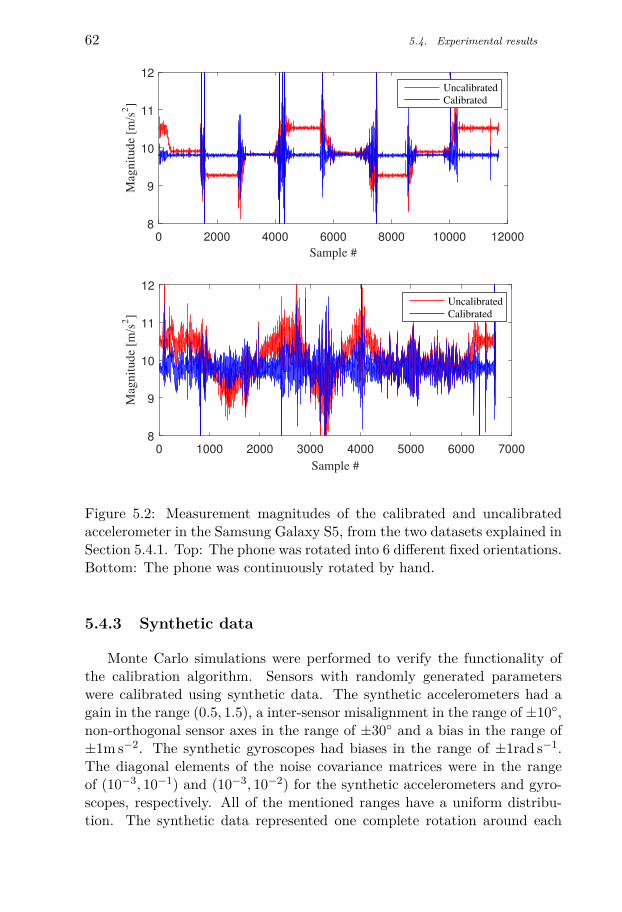
62 5.4. Experimental results
Sample #
0 2000 4000 6000 8000 10000 12000
Mag
nit
ude
[m/s
2]
8
9
10
11
12
Uncalibrated
Calibrated
Sample #
0 1000 2000 3000 4000 5000 6000 7000
Mag
nit
ud
e [m
/s2]
8
9
10
11
12
Uncalibrated
Calibrated
Figure 5.2: Measurement magnitudes of the calibrated and uncalibratedaccelerometer in the Samsung Galaxy S5, from the two datasets explained inSection 5.4.1. Top: The phone was rotated into 6 different fixed orientations.Bottom: The phone was continuously rotated by hand.
5.4.3 Synthetic data
Monte Carlo simulations were performed to verify the functionality ofthe calibration algorithm. Sensors with randomly generated parameterswere calibrated using synthetic data. The synthetic accelerometers had again in the range (0.5, 1.5), a inter-sensor misalignment in the range of ±10◦,non-orthogonal sensor axes in the range of ±30◦ and a bias in the range of±1m s−2. The synthetic gyroscopes had biases in the range of ±1rad s−1.The diagonal elements of the noise covariance matrices were in the rangeof (10−3, 10−1) and (10−3, 10−2) for the synthetic accelerometers and gyro-scopes, respectively. All of the mentioned ranges have a uniform distribu-tion. The synthetic data represented one complete rotation around each

Paper I – Accelerometer calibration using sensor fusion with a gyroscope 63
Sample #
0 50 100 150 200 250 300 350 400
Mag
nit
ude
[m/s
2]
6
8
10
12
14
Sample #
0 50 100 150 200 250 300 350 400
Angula
r er
ror
[deg
rees
]
0
10
20
30
40
Figure 5.3: Calibrated and uncalibrated measurement magnitudes and an-gular errors for 1000 Monte Carlo simulations. The blue lines represent thecalibrated measurements ycal
t , and the red lines represent the uncalibratedmeasurements yt. The means are represented as solid lines with a confidenceinterval of one standard deviation, represented by the dashed lines.
axis. A total of 1000 simulations were performed.
The difference between the calibrated and uncalibrated measurementscan be seen in Fig. 5.3. After calibration, the magnitude of the measure-ments are significantly closer to the true magnitude ‖g‖2 = 9.82m s−2. Theabsolute value of the angle between the calibrated measurement vectorsycalt , and the ideal (noise- and error free) measurement vectors (the angular
error), also decreased to an average of 2 degrees. The average absolute ori-entation estimation errors also decreased significantly from 8.3(σ = 7.1)◦ to0.32(σ = 0.40)◦ for the roll angle, and from 8.3(σ = 6.9)◦ to 0.33(σ = 0.43)◦for the pitch angle. To speed up these simulations, the Gauss-Newtonmethod was allowed to perform a maximum of 10 iterations. However, thealgorithm converged in 6 iterations or less on average.

64 5.5. Conclusions
Parameter #
1 2 3 4 5 6 7 8 9 10 11 12
RM
SE
×10-3
0
2
4
RMSE
sqrt(CRLB)
Figure 5.4: Square root of the estimated CRLB and the RMSE for theestimated parameters for 100 simulations using the same set of parameters.The first 9 parameters belong to the vectorized matrix D and parameters10-12 belong to the bias vector ba.
5.4.4 Cramér-Rao lower bound
A common tool used to evaluate the performance of estimators is theCramér-Rao lower bound (CRLB), which gives a lower bound on the vari-ance of an unbiased estimator (Gustafsson 2010). The CRLB was calcu-lated using the mean Hessian from 100 simulations using one fixed set ofparameters. The square root of the CRLB can be compared with the root-mean-square error (RMSE), for the estimated parameters θ, see Fig. 5.4.The RMSE values were found to be close to the square root of the estim-ated CRLB which suggests that the estimator is efficient. Interestingly, forparameter 6, it can be seen that
√CRLB > RMSE. This could be because
of the numerical approximation of the CRLB or because there is a smallbias in the parameter estimates.
5.5 Conclusions
In this paper, a calibration method for a triaxial accelerometer, usingsensor fusion with a triaxial gyroscope in the same platform, has been presen-ted. The main goal of the method is to allow sensor platforms with lowerquality sensors, e.g. smartphones, to be used in applications which requirehigher accuracy measurements. The method has been tested using both realand synthetic data, and has been shown to accurately calibrate the sensors.The estimated parameters can be used to compensate for gain, inter-sensormisalignment, non-orthogonal sensor axes, cross-axis interference and bias.The method was used to calibrate the accelerometer in a smartphone, whichbrought the measurement magnitudes closer to ‖g‖2. This was a signific-

Paper I – Accelerometer calibration using sensor fusion with a gyroscope 65
ant improvement compared to the uncalibrated accelerometer, where themagnitudes varied for different orientations. It was also shown that the cal-ibration works when using a smartphone to perform orientation estimation,improving the accuracy in the estimated roll and pitch angles. Monte Carlosimulations show a significantly reduced effect of sensor errors in the cal-ibrated measurements. Simulations also showed that the RMSE was closeto the
√CRLB for the estimated parameters, which suggests that the Max-
imum likelihood estimator is efficient. The Gaussian noise model used herecannot describe measurement outliers.
We see a number of interesting improvements and extensions of themethod. The problem of too many outliers could be handled by differ-ent approaches: outlier detection, by using a heavytailed noise distributionor by using robust Kalman filtering (Mattingley and Boyd 2010). Anotherpossible future extension would be to combine the method with magneto-meter calibration for more accurate heading estimates. In addition to theseimprovements, further analysis with sensors of varying quality, and compar-isons to other methods would be interesting as future work.

66 References
ReferencesBoyd, S. and L. Vandenberghe (2004). Convex optimization. Cambridge uni-
versity press.Fang, B., W. Chou and L. Ding (2014). ‘An Optimal Calibration Method
for a MEMS Inertial Measurement Unit’. In: International Journal ofAdvanced Robotic Systems 11, pp. 1–14.
Forsberg, T., N. Grip and N. Sabourova (2013). ‘Non-iterative calibrationfor accelerometers with three non-orthogonal axes, reliable measurementsetups and simple supplementary equipment’. In: Measurement Scienceand Technology 24.3, p. 035002.
Frosio, I., F. Pedersini and N. A. Borghese (June 2012). ‘Autocalibration ofTriaxial MEMS Accelerometer With Automatic Sensor Model Selection’.In: IEEE Sensors Journal 12.6, pp. 2100–2108.
Grip, N. and N. Sabourova (2011). ‘Simple non-iterative calibration for tri-axial accelerometers’. In: Measurement Science and Technology 22.12,p. 125103.
Gustafsson, F. (2010). Statistical sensor fusion. Studentlitteratur.InvenSense (Sept. 2017). 6 Axis MotionTracking. url: http : / / www .
invensense.com/products/motion-tracking/6-axis/.Kok, M. (2014). Probabilistic modeling for positioning applications using
inertial sensors. Licentiate’s thesis, Linköping University, Sweden.Kok, M. and T. B. Schön (Aug. 2014). ‘Maximum likelihood calibration of a
magnetometer using inertial sensors’. In: Proceedings of the 19th WorldCongress of the International Federation of Automatic Control (IFAC).Cape Town, South Africa, pp. 92–97.
Mattingley, J. and S. Boyd (May 2010). ‘Real-Time Convex Optimization inSignal Processing’. In: IEEE Signal Processing Magazine 27.3, pp. 50–61.
Olsson, F., M. Kok, K. Halvorsen and T. B. Schön (2016). ‘Accelerometercalibration using sensor fusion with a gyroscope’. In: Statistical SignalProcessing Workshop (SSP), 2016 IEEE. (Palma de Mallorca, Spain).IEEE, pp. 1–5.
Panahandeh, G., I. Skog and M. Jansson (Sept. 2010). ‘Calibration of the Ac-celerometer Triad of an Inertial Measurement Unit, Maximum LikelihoodEstimation and Cramér-Rao Bound’. In: Procceedings of the Interna-tional Conference on Indoor Positioning and Indoor Navigation (IPIN).Zurich, Switzerland, pp. 1–6.
Särkkä, S. (2007). Notes on quaternions. Tech. rep. Helsinki University ofTechnology.
Serrano, D. E. and F. Ayazi (2015). ‘Resonant MEMS: Fundamentals, Imple-mentation, and Application’. In: ed. by O. Brand, I. Dufour, S. Heinrich,

Paper I – Accelerometer calibration using sensor fusion with a gyroscope 67
F. Josse, G. K. Fedder, C. Hierold, J. G. Korvink and O. Tabata. Wiley-VCH. Chap. MEMS Inertial Sensors, pp. 329–352.
Won, S. P. and F. Golnaraghi (Aug. 2010). ‘A Triaxial accelerometer Cal-ibration Method Using a Mathematical Model’. In: IEEE Transactionson Instrumentation and Measurement 59.8, pp. 2144–2153.
Woodman, O. J. (Aug. 2007). An introduction to inertial navigation. Tech.rep. 696. University of Cambridge Computer Laboratory.
Wright, S. and J. Nocedal (2006). Numerical Optimization. 2nd. SpringerSeries in Operations Research.

68 References

Paper II
TitleExperimental evaluation of joint position estimation using inertial sensors
AuthorsFredrik Olsson and Kjartan Halvorsen
Edited version ofF. Olsson and K. Halvorsen (2017). ‘Experimental evaluation of joint positionestimation using inertial sensors’. In: Information Fusion (Fusion), 2017 20thInternational Conference on. (Xi’an, China). IEEE, pp. 1–8

70
Experimental evaluation ofjoint position estimationusing inertial sensors
Abstract
In this paper we study the problem of estimating the position of a jointthat is connecting two rigid links in a biomechanical model. By equip-ping the two links with inertial sensors, which measure linear accelerationand angular velocity, it is possible to estimate the joint position. Estimationmethods for this problem have been proposed before, but experimental eval-uation and comparison between methods is lacking. The main contributionof this paper is an experimental evaluation of three different methods, aleast-squares method and two iterative optimization methods that minimizea sum of squared errors and a sum of absolute errors. The iterative methodsturns out to be superior to the least-squares method. Minimizing the sumof squared errors is faster but not as robust against outliers as minimizingthe sum of absolute errors.
6.1 Introduction
Inertial sensors, specifically triaxial accelerometers and gyroscopes whichmeasure linear acceleration and angular velocity in three dimensions, arewidely available in our everyday lives. As microelectromechanical systems(MEMS), inertial sensors are staple components in today’s smart phonesand other wearable devices such as activity monitors, smart wristbands andwatches. This has made inertial sensors attractive tools for analysing humanmotion, for example to perform full body motion capture (Roetenberg et al.2013), quantifying symptoms of diseases, tracking the progress of rehabilit-ation (Patel et al. 2012) or aiding elite sportsmen in their training (James2006). In all of these applications, an important problem to consider is
71

72 6.2. Modeling
how the measurements from the sensors relate to the human body. A hu-man body can be approximated as separate links that connect to each otherthrough joints that allow the links to move in certain ways with respect toeach other. Such a model of a human is what we refer to as a biomechan-ical model. Establishing the relationship between the inertial sensors andlinks and joints of the biomechanical model is referred to as calibrating thebiomechanical model, and it is often a necessary step in the mentioned ap-plications.
In this paper we consider the problem of estimating the position of a jointconnecting two links in the biomechanical model. One inertial sensor will beattached to each link. We assume the positions of the sensors to be fixed withrespect to the center of the joint, but apart from this there will be no furtherprior knowledge assumed about the positions and orientations of the sensors.When the position of the joint center is fixed with respect to the referenceframe of the sensors, it is possible to estimate the position of the joint usingthe measurements from the two inertial sensors. Similar problems havebeen studied previously in e.g. Crabolu et al. (2016), McGinnis and Perkins(2013) and Seel et al. (2012), but experimental evaluation and comparisonsof the methods are lacking. Our main contribution with this paper is theexperimental evaluation of three possible methods for estimating the jointposition using the two inertial sensors. Evaluations were made using a rathersimple experimental system, an artificial limb consisting of two rigid linksconnected by a spherical joint.
6.2 Modeling
6.2.1 Relating the inertial measurements to the biomechan-ical model
Let L1 and L2 denote local (Cartesian) reference frames that are fixedin sensor 1 and 2, respectively, and G denote a global earth-fixed refer-ence frame. The measured accelerations a relate to the measured angularvelocities ω and the angular accelerations ω in the following way
a1 = aL10 + ω1 × (ω1 × r1) + ω1 × r1 (6.1)
a2 = aL20 + ω2 × (ω2 × r2) + ω2 × r2, (6.2)
where a0 is the linear acceleration of the center of rotation expressed inL1 and L2, respectively, as indicated by the superscripts. The measuredaccelerations, angular velocities and angular accelerations, are expressed inthe local reference frame associated with the subscripts. A similar notationis used for the position of the joint, r, when expressed in the local reference
Paper II – Experimental evaluation of joint position estimation using inertial sensors 73
frames. The described model is illustrated in Figure 6.1. We can rewrite(6.1)-(6.2) as
a1 = aL10 +K(ω1, ω1)r1 (6.3)
a2 = aL20 +K(ω2, ω2)r2, (6.4)
where
K(ω, ω) =
−ω2
y − ω2z ωxωy − ωz ωxωz + ωy
ωxωy + ωz −ω2x − ω2
z ωyωz − ωxωxωz − ωy ωyωz + ωx −ω2
x − ω2y
, (6.5)
where the x, y, z subscripts denote the coordinates of the three dimensionalvectors. To simplify notation we will use K(ω1, ω1) = K1 and K(ω2, ω2) =K2.
6.2.2 Measurement models
The accelerometers and gyroscopes provide us with noisy measurementsof the accelerations and the angular velocities. Simple models of the meas-urements at sample instant k are given by
ya(k) = a(k) + ea,k, ea,k ∼ N (0,Σa) (6.6)yω(k) = ω(k) + eω,k, eω,k ∼ N (0,Σω), (6.7)
where we say that the measurement is equal to the physical quantity plussome additive Gaussian measurement noise. Inertial sensors, especially lowerquality sensors, tend to also have a time varying bias, causing the measure-ments to slowly drift over time. A simple way to estimate the bias is tocollect data from stationary sensors and see how much they differ from theexpected stationary accelerations and angular velocities. This initially es-timated bias can then be assumed to be stationary over short time periodsand removed from the data. Angular accelerations are also needed by themethods, and these must be estimated from the gyroscope measurements.We will use a simple second-order symmetric difference quotient
ω(k) ≈ yω(k) = yω(k + 1)− yω(k − 1)2h , (6.8)
where h is the sample period. Other, higher order differentiation techniquesmay also be used. When estimating the position of the joint we will makeuse of these noisy measurements, so when we refer to a, ω and ω in theupcoming sections we will mean the measurements given by (6.6)-(6.8) andnot the true physical quantities.

74 6.3. Estimation
ω1
ω2
a0
a1
a2
r1
r2
GL1
L2
x y
zz
yx
x
y z
Figure 6.1: The biomechanical model and inertial sensors, where the jointpositions with respect to the sensors, r1 and r2 are to be estimated.
6.3 Estimation
6.3.1 Least-squares estimate
Note that (6.3)-(6.4) is linear in a0 and r =[r1 r2
]>. Let R1,2 denote
the rotation matrices which rotates vectors expressed in the L1,2 frames tothe G frame. For example we have that
R1aL10 = aG0 .

Paper II – Experimental evaluation of joint position estimation using inertial sensors 75
By using these rotation matrices we can express (6.3)-(6.4) in the G frame
R1a1 −R2a2 = aG0 − aG0 +R1K1r1 −R2K2r2
= R1K1r1 −R2K2r2, (6.9)
which is a system of equations which is linear in r. Once both accelera-tions are expressed in a common reference frame, a0 is eliminated from theequation by subtracting one acceleration from the other. With a set of Navailable measurements, the following system of equations can be construc-ted
Kr = a (6.10)
K =
K(1)...
K(N)
=
R1(1)K1(1) −R2(1)K2(1)
......
R1(N)K1(N) −R2(N)K2(N)
(6.11)
a =
a(1)...
a(N)
=
R1(1)a1(1)−R2(1)a2(1)...
R1(N)a1(N)−R2(N)a2(N)
, (6.12)
where K ∈ R3N×6 and a ∈ R3N×1. A least-squares (LS) estimate of r canbe found by minimizing a cost function which corresponds to the sum ofsquared errors of the linear equations
rLS = arg minr
N∑
k=1
∥∥∥K(k)r − a(k)∥∥∥
2
2, (6.13)
which has the closed form solution
rLS = K†a, (6.14)
where † denotes the Moore-Penrose pseudo inverse.The rotation matrices R1,2 can be found by estimating the orientation
of the inertial sensors with respect to G. There are several methods thatone can use to estimate the orientations of the inertial sensors (Kok 2016),and some inertial sensors include internally computed orientation estimates.However, since estimates of R1,2 are needed to compute rLS this introducesan additional source of uncertainty that can be hard to quantify. It should benoted that the LS approach presented here extends the methods presentedin McGinnis and Perkins (2013) and Crabolu et al. (2016). These methodsassume that a0 = 0, which would allow for separate estimation of r1 and r2without having to know the orientation of the sensors. There are not manyscenarios where the assumption that the center of the joint is at rest holdswhen studying human motion, however. So it is less restrictive and morepractical to consider the case when a0 6= 0.

76 6.3. Estimation
6.3.2 Estimation using iterative optimization methods
Another way of estimating r is to use iterative optimization methods.The method proposed in Seel et al. (2012) minimizes a sum of squared errors(SS) cost function
rSS = arg minr
N∑
k=1e(k, r)2 (6.15)
e(k, r) = ‖a1(k)−K1(k)r1‖2 − ‖a2(k)−K2(k)r2‖2 , (6.16)
where ‖·‖2 stands for the Euclidean norm. A nice property of defining theerrors e(k, r) as the difference between two Euclidean norms is that theEuclidean norm is invariant to rotations. Therefore, unlike the LS method,we do not need to estimate the orientation of the sensors to remove a0 fromthe equation since ‖aL1
0 ‖2 = ‖aL20 ‖2. The optimization problem (6.15) can be
solved efficiently using a Gauss-Newton method (Wright and Nocedal 2006)as shown in Seel et al. (2012), which makes use of the partial derivatives
∂e(k, r)∂r1
= −K1(k)>e1(k, r1)‖e1(k, r1)‖2
(6.17)
∂e(k, r)∂r2
= K2(k)>e2(k, r2)‖e2(k, r2)‖2
, (6.18)
where
ei(k, ri) = ai(k)−Ki(k)ri, i = 1, 2. (6.19)
An alternative to minimizing the sum of squared errors is to insteadminimize the sum of absolute errors (SA)
rSA = arg minr
N∑
k=1|e(k, r)|. (6.20)
A well known property of this type of cost function is robustness against out-liers in the data since large residuals are weighted by their absolute value,not by their squared value in the cost function. By outliers we mean meas-urements that contain some sort of disturbance that the model does nottake into account. One common disturbance comes from the fact that hu-man body segments are non-rigid. The sensors are placed on soft tissue,sometimes with clothing between the sensors and the skin. This violates theassumption that the sensor position with respect to the joint is fixed at alltimes since the surface on which the sensors are placed can move to somedegree. These types of disturbances are known as soft tissue artifacts (STA)
Paper II – Experimental evaluation of joint position estimation using inertial sensors 77
(Leardini et al. 2005). Since the optimization problem given by (6.20) isnot a sum of squares minimization problem, it is not possible to use theGauss-Newton method to solve this optimization problem. Other gradientdescent-type methods (Boyd and Vandenberghe 2004) may be used, whichrequire the partial derivatives (subgradients)
∂|e(k, r)|∂r1
= −sgn(e(k, r))K1(k)>e1(k, r1)‖e1(k, r1)‖2
(6.21)
∂|e(k, r)|∂r2
= sgn(e(k, r))K2(k)>e2(k, r2)‖e2(k, r2)‖2
, (6.22)
where
sgn(x) =
−1 x < 00 x = 01 x > 0
. (6.23)
It is important to note that neither of the estimation methods describedin this section guarantee that a unique solution exists in general. If thedata contains unmodeled disturbances or outliers, multiple solutions or localminima may exist. The resulting estimates may then in some cases describethe outliers rather than the kinematics of the model of interest.
6.4 ExperimentAn experiment was performed using a system consisting of two rigid
cylindrical links joined together by a spherical joint, which allows the linksto rotate with up to two degrees of freedom with respect to each other. TwoXsens MTw Awinda wireless inertial sensors (Xsens 2017) were placed nearthe ends of the links. The setup of the experimental system can be seen inFigure 6.2. The links are rigid such that the position of the joint relative tothe sensors can be considered fixed for the full duration of the experiment.The positions of the joint relative to the sensors were measured beforehandto be
r1 =[334 0 28
]>(±2) (6.24)
r2 =[−325 0 28
]>(±2), (6.25)
expressed in the L1,2 frames in millimeters. The experiment consisted ofcollecting inertial measurements while picking up the system and performingcertain motions by hand. The sample rates of the sensors were 100 Hz anda total of 15219 data samples were collected during the experiment. The

78 6.4. Experiment
Figure 6.2: The system that was used in the experiment with two XsensMTw inertial sensors attached.
data can be divided into segments Si, i = 1, 2, . . . , 8, each of which containsone specific type of motion, see Figure 6.3. The motions contained in eachsegment are:
S1: The system was at rest on a flat surface. This segment was used tocalibrate gyroscope bias and noise covariance. Contains 1354 samples.
S2: The system was picked up and held such that the two segments werein an approximately vertical orientation. Contains 1132 samples.
S3: The links were moved back and forth with respect to the joint. Themajority of the rotation aligned with the y−axes of the sensors. Con-tains 1625 samples.
S4: The links were moved back and forth with respect to the joint. Themajority of the rotation aligned with the z−axes of the sensors. Con-tains 1372 samples.
S5: The links were moved back and forth with respect to the joint. Al-ternated rotations around the y− and z−axes of the sensors. Contains2213 samples.
S6: The links were spun such that the bottom link followed an approx-imately clockwise circular trajectory. The system was flipped upsidedown in the middle of the segment and the motion repeated. Contains2666 samples.
S7: Same as S6 but counter-clockwise motion. Contains 2698 samples.
S8: The system was placed back on the flat surface as in S1. Contains2159 samples.

Paper II – Experimental evaluation of joint position estimation using inertial sensors 79
0 50 100 150
Time [s]
-20
-10
0
10
20Acceleration[m
/s2]
Accelerometer 1
S1
S2
S3
S4
S5
S6
S7
S8
0 50 100 150
Time [s]
-10
-5
0
5
10
Angularvelocity
[rad/s]
Gyroscope 1
S1
S2
S3
S4
S5
S6
S7
S8
Figure 6.3: Data collected from sensor 1 during the experiment.
6.5 Results
6.5.1 Metrics for evaluation of estimators
The performance of the estimators are evaluated in terms of the averageEuclidean error and its standard deviation
Eavg(ri) = 1M
M∑
j=1Ej(ri), i = 1, 2 (6.26)
Std [Ej(ri)] =
√√√√ 1M
M∑
j=1(Ej(ri)− Eavg(ri))2 (6.27)
Ej(ri) = ‖ri(j)− ri‖2 , (6.28)
where Ej(ri) denotes the Euclidean norm of the error for the j :th estim-ate of ri. The average Euclidean error Eavg(ri) and its standard deviationStd [Ej(ri)] are computed for a total of M estimates. The rationale forchoosing the average Euclidean error over e.g. the more commonly usedroot mean square error (RMSE) is that it may be interpreted as the averagephysical distance between estimates with respect to the true joint center (Li

80 6.5. Results
and Zhao 2006). This results in a more intuitive understanding as to howclose the estimators are to estimating the true position of the joint center.The standard deviation of the Euclidean error give us information about thevariation or consistency of the estimates.
6.5.2 Method verification using simulated data with idealexcitation
To see that the methods were correctly implemented and working we firstused simulated measurements for estimating r1,2. Angular velocities andangular accelerations were randomly generated from zero-mean Gaussiandistributions with standard deviations of 10 rad/s and 10 rad/s2, respect-ively. Accelerometer measurements were then generated from the models(6.1) and (6.2) using the measured sensor positions (6.24) and (6.25). Theaccelerations of the joint a0 were uniformly random rotations of the gravita-tional acceleration vector g =
[0 0 9.82
]>. Additive zero-mean Gaussian
noise with variances 10−2 m2/s4, 10−5 rad2/s2 and 5 × 10⁻² rad2/s4, wereadded to the accelerations, angular velocities and angular accelerations, re-spectively. The first two noise levels are typical for the accelerometers andgyroscopes found in the Xsens MTw sensors, and the noise added to theangular accelerations takes into account the second order finite differencequotient that is used to differentiate the noisy gyroscope signals. In addi-tion to measurement noise, orientation errors were simulated as zero-meanGaussian random variables with a standard deviation of 5◦. By allowingthe angular velocities and angular accelerations to be randomly generatedlike this, we do not take constraints of the real biomechanical model intoaccount, such as the physically possible range of motion. The randomly gen-erated measurements give us an indication of how well the methods wouldperform if the system could be ideally excited, with no constraints limit-ing the motion. A total of M = 100 estimation runs were performed usingN = 500 randomly generated measurements in each run. The results forthese runs are shown in Table 6.1.
6.5.3 Estimation using the experimental data
The joint positions r1,2 were estimated using the data collected from theexperiment described in Section 6.4. At first, estimation was done using datafrom segments S3 to S7. To avoid using non-informative stationary data, athreshold of 1.2 rad/s was used to exclude all samples where the norm ofthe gyroscope measurement was below this threshold. This threshold wasalso used in all subsequent estimations. As a result, a total of N = 6280measurements were selected from the segments S3 to S7. Using the same
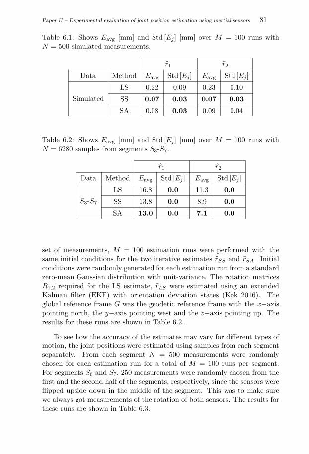
Paper II – Experimental evaluation of joint position estimation using inertial sensors 81
Table 6.1: Shows Eavg [mm] and Std [Ej ] [mm] over M = 100 runs withN = 500 simulated measurements.
r1 r2
Data Method Eavg Std [Ej ] Eavg Std [Ej ]
SimulatedLS 0.22 0.09 0.23 0.10SS 0.07 0.03 0.07 0.03SA 0.08 0.03 0.09 0.04
Table 6.2: Shows Eavg [mm] and Std [Ej ] [mm] over M = 100 runs withN = 6280 samples from segments S3-S7.
r1 r2
Data Method Eavg Std [Ej ] Eavg Std [Ej ]
S3-S7
LS 16.8 0.0 11.3 0.0SS 13.8 0.0 8.9 0.0SA 13.0 0.0 7.1 0.0
set of measurements, M = 100 estimation runs were performed with thesame initial conditions for the two iterative estimates rSS and rSA. Initialconditions were randomly generated for each estimation run from a standardzero-mean Gaussian distribution with unit-variance. The rotation matricesR1,2 required for the LS estimate, rLS were estimated using an extendedKalman filter (EKF) with orientation deviation states (Kok 2016). Theglobal reference frame G was the geodetic reference frame with the x−axispointing north, the y−axis pointing west and the z−axis pointing up. Theresults for these runs are shown in Table 6.2.
To see how the accuracy of the estimates may vary for different types ofmotion, the joint positions were estimated using samples from each segmentseparately. From each segment N = 500 measurements were randomlychosen for each estimation run for a total of M = 100 runs per segment.For segments S6 and S7, 250 measurements were randomly chosen from thefirst and the second half of the segments, respectively, since the sensors wereflipped upside down in the middle of the segment. This was to make surewe always got measurements of the rotation of both sensors. The results forthese runs are shown in Table 6.3.

82 6.5. Results
Table 6.3: Shows Eavg [mm] and Std [Ej ] [mm] over M = 100 runs withN = 500 randomly picked samples from different segments.
r1 r2
Data Method Eavg Std [Ej ] Eavg Std [Ej ]
S3
LS 332.7 19.4 181.8 18.3SS 17.5 0.5 6.6 0.4SA 17.5 2.3 6.8 1.6
S4
LS 806.5 13.4 655.5 11.5SS 15.9 0.4 5.1 0.3SA 15.0 1.3 6.0 0.7
S5
LS 325.6 23.4 129.3 27.5SS 13.8 0.5 6.8 0.5SA 13.0 1.3 7.3 1.0
S6
LS 40.0 6.4 33.9 10.5SS 24.2 23.6 10.7 8.8SA 13.1 0.2 7.4 0.3
S7
LS 20.9 8.1 21.1 7.1SS 22.4 12.7 9.4 2.4SA 13.0 0.3 7.1 0.3
6.5.4 Estimation with simulated soft tissue artifacts
In this experiment we investigated how the methods performed whenthe inertial measurements were corrupted by disturbances. Possible dis-turbances when analysing real human motion may appear in the form ofSTAs. Since the links in the experimental system are rigid we simulatedthese disturbances. A model that has been shown to emulate STAs in thethigh reasonably well expresses the displacement of markers attached tothe skin as a linear combination of the hip joint angles (Camomilla et al.2013). Differentiating this model twice w.r.t. time yields a linear relation-ship between the linear acceleration of the displacement of skin and theangular acceleration. Using this model structure as a basis, we generatedSTAs as an additive disturbance to the acceleration measurements as a linearcombination of the angular acceleration measurements
da = Hω, (6.29)

Paper II – Experimental evaluation of joint position estimation using inertial sensors 83
Table 6.4: Shows Eavg [mm] and Std [Ej ] [mm] over M = 100 runs withN = 6280 samples from segments S3-S7. With simulated disturbances addedto the accelerometer measurements.
r1 r2
Data Method Eavg Std [Ej ] Eavg Std [Ej ]
S3-37
LS 31.6 12.2 22.7 12.4SS 17.6 5.6 11.2 4.2SA 15.2 3.7 10.4 4.0
where H is a 3×3 matrix containing the STA model parameters. In practice,the elements of H depend on multiple factors such as sensor placement andthe physiology of the person. Therefore, the elements of H were random-ized from a zero-mean Gaussian distribution with a standard deviation of18π mm/rad at the start of each estimation run. This generated H matriceswith elements of a magnitude comparable to what was found in (Camomillaet al. 2013). A total of M = 100 estimation runs were performed using thesame N = 6280 samples from segments S3 to S7 that were used to producethe results shown in Table 6.2. The results for these runs are shown inTable 6.4.
6.5.5 Analysis of the cost functions of the iterative method
Throughout the estimation runs we found that the iterative methodsperformed significantly worse than expected for certain parts of the data,see Table 6.3. We analyzed how the cost functions (6.15) and (6.20) dependon the values of the x-coordinates of r1 and r2 in a small neighborhoodaround the true joint positions r1 and r2. Figure 6.4 show the level curvesof the cost functions for a specific set of data from one estimation run using250 random samples from the first half and 250 random samples from thesecond half of the S6 segment. Similarly, Figure 6.5 show the level curves ofthe cost functions, but when using 500 random samples from the first halfof the S6 segment instead.
From Figure 6.4 we see that the SS cost function has two distinct localminima for this specific set of data, while the SA cost function only hasone global minima. This would explain why the standard deviations ofthe SS estimates were significantly larger compared to the SA estimates forsegments S6 and S7. It is clear from this example that some of the randomdata samples picked during the estimation runs can cause multiple localminima to appear. The Gauss-Newton method will then converge to the

84 6.6. Discussion
local minima closest to the initial estimate.Figure 6.5 show us what happens when the majority of the data consists
of rotations of only one of the sensors. We see that the cost functions aremuch steeper in the r2 direction than the r1 direction since the first half ofthe S6 segment consists mostly of rotations of the second sensor. A problemthat may happen in cases such as these is that the iterative methods mayconverge to an r1 coordinate that is anywhere in the valley, since the levelcurves of the cost function are nearly flat in one direction. This shows howimportant it is to choose data where both sensors have been sufficientlyexcited by the motion.
6.6 Discussion
6.6.1 Motion is important
The functionality of the three estimators was verified by the resultsshown in Table 6.1, where measurements were simulated with an ideal excit-ation. However, a motion that would allow for such excitation is impossibleto perform under the conditions presented by our experimental setup and inmost scenarios involving human motion due to limitations in mobility. Theexperimental data we collected contains multiple different types of motion,and even when using data from segments S3-S7, the average Euclidean errorincreases for all three estimators as shown by the results in Table 6.2 whencompared to Table 6.1. All three estimators were consistent when usingthe data from the S3-S7 segments however, as is evident from the standarddeviations, which were smaller than 0.05 mm.
The importance of the motion becomes clearer from the results shown inTable 6.3, where data was randomly picked from single segments. The errorsvary significantly across the five segments. The LS estimator in particularshow poor performance for segments S3-S5. The motion during those seg-ments is mostly constrained to one or two planes which makes the K-matrixfrom (6.5) close to singular, causing numerical issues when computing the LSestimate. In Section 6.5.5 we also showed the importance of having sufficientrotation of both sensors as the cost functions tend to become flat in somedirection otherwise, as shown in Figure 6.5. Therefore, the best strategy isto combine multiple types of motion which allows rotation of both sensors.
6.6.2 The main difference of the estimators lies in the costfunctions
The three estimators minimize different cost functions to find an estim-ate of r. The cost functions are similar in the sense that they consist of sums

Paper II – Experimental evaluation of joint position estimation using inertial sensors 85
SS cost function
-400 -350 -300 -250 -200
r2,x [mm]
200
220
240
260
280
300
320
340
360
380
400
r1,x[m
m]
600
800
1000
1200
1400
1600
SA cost function
-400 -350 -300 -250 -200
r2,x [mm]
200
220
240
260
280
300
320
340
360
380
400
r1,x[m
m]
200
250
300
350
400
450
500
Figure 6.4: The level curves of the SS and SA cost functions in a neighbor-hood around the true x−coordinates. Using N = 500 random samples fromboth halves of segment S6.
of errors that should go to zero as the relationships in (6.1)-(6.2) becomesatisfied. However, our measurements are corrupted by noise and possibly

86 6.6. Discussion
SS cost function
-400 -350 -300 -250 -200
r2,x [mm]
200
220
240
260
280
300
320
340
360
380
400
r1,x[m
m]
100
200
300
400
500
600
700
800
900
SA cost function
-400 -350 -300 -250 -200
r2,x [mm]
200
220
240
260
280
300
320
340
360
380
400
r1,x[m
m]
100
150
200
250
300
350
400
450
500
550
Figure 6.5: The level curves of the SS and SA cost functions in a neighbor-hood around the true x−coordinates. Using N = 500 random samples fromonly the first half of segment S6.
other disturbances that are not taken into account by the model. Meas-urements that deviate significantly from the model, so called outliers, could

Paper II – Experimental evaluation of joint position estimation using inertial sensors 87
have a significant impact on the estimates depending on how the errors aredefined in the cost functions.
The LS (6.13) and the SS (6.15) cost functions model the errors dif-ferently. The LS cost function have errors that are linear in the unknownparameter r, but requires additional information about the orientation ofthe sensors, while the SS cost function have errors that are nonlinear in r,but are invariant to the orientation. What the LS and SS estimators have incommon is that they seek to minimize the sum over squared errors, whichgives these estimators some nice numerical properties. The LS estimateshave a closed form solution, which can be computed efficiently. The SSestimates can be found using a Gauss-Newton method, which typically con-verges faster than gradient descent methods, since information about theHessian of the cost function is utilized. However, since the cost functionscontain the squared errors, it also means that large errors can have a sig-nificant impact on the estimates. Outliers can give rise to multiple localminima as in Figure 6.4, and may pull the estimates away from the truequantity, which will be discussed further in Section 6.6.4.
The SA cost function (6.20) models the errors similarly to the SS costfunction, but contains a sum of the absolute errors rather than the squarederrors. Outliers will therefore have a less significant impact on the value ofthe cost function, and will thus affect the estimates less. However, the SAcost function requires more effort to find its minimum compared to the SScost function. The Hessian of the SA cost function cannot be formed sincethe absolute value is not differentiable in the origin, and we have to rely solelyon the information of the subgradients, resulting in slower convergence.
6.6.3 The least-squares estimator relies on accurate orienta-tion estimates
Another important distinction of the LS estimator is that it requires ori-entation estimates in the form of the rotation matrices R1,2. An EKF withorientation deviation states (Kok 2016) was used to obtain orientation estim-ates for the whole data set. In essence, this type of EKF uses the gyroscopemeasurements to track the dynamic rotation of an inertial sensor. Since thisinvolves integrating noisy measurements, the orientation estimates will havean error that increases in magnitude over time. To compensate for this, theEKF may also incorporate measurements from an accelerometer and/or amagnetometer. A stationary accelerometer measures the local gravitationalacceleration, which is an observation of the sensor’s inclination and a mag-netometer measures the Earth magnetic field which is an observation of theheading. However, to incorporate these measurements in the EKF one hasto make some assumptions.

88 6.6. Discussion
The accelerometer is assumed to be stationary, which is clearly not thecase for most of our data. Therefore, only accelerometer measurements ofmagnitude within ±5% of the magnitude of the local gravitational accel-eration is used as an observation of inclination in the EKF. Choosing thisthreshold is important. A small threshold may cause the integration errorto grow, since there will be fewer inclination observations available. Onthe other hand, a large threshold include more erroneous inclination obser-vations since the assumption of a stationary sensor is violated more. Wefound 5% to be a good threshold for this data set. However, while tuningthis threshold we found that the LS estimation errors varied significantly,which indicates that the LS estimator is sensitive to the orientation estim-ates. A good strategy could be to record a motion that allows the sensorto be close to stationary at regular intervals. A smaller threshold couldthen be used since the data set is designed to include regular inclinationobservations, while excluding most data that violates the assumption of astationary sensor.
The Xsens MTw sensors used also include magnetometers which couldbe used to obtain heading observations. However, magnetometers measuremagnetic disturbances in addition to the Earth magnetic field, which makesthem unreliable in certain environments. We found that only using mag-netometer measurements from the S1 segment to obtain an initial headingof the sensors, but not using the magnetometer measurements as headingobservations in the EKF, worked best for our data set.
If we represent the unknown orientation estimation errors as rotationmatrices E1,2 equation (6.9) is not satisfied. We get
E1R1a1 − E2R2a2 == (E1 − E2)aG0 + E1R1K1r1 − E2R2K2r2
6= E1R1K1r1 − E2R2K2r2, (6.30)
where the unknown acceleration of the joint center a0 remains in the equa-tion. Large orientation estimation errors in combination with large acceler-ations of the joint center are therefore detrimental to the LS estimator. Asmentioned in Section 6.5.3, we only used measurements where the magnitudeof the gyroscope measurement was larger than 1.2 rad/s. This thresholdalso turned out to be important for the LS estimator. It is clear from (6.30)that the K1,2 matrices carry information about r1,2. Since K1,2 dependon the angular velocities and angular accelerations, choosing to only usemeasurements of sufficiently large magnitude may suppress the error term,(E1 − E2)aG0 in (6.30).
The additional work needed to tune an orientation estimation methodto work well with a particular data set may be seen as a disadvantage of

Paper II – Experimental evaluation of joint position estimation using inertial sensors 89
the LS estimator when compared to the SS and SA estimators. However, itis possible that a better strategy for tuning the orientation estimation andselecting a threshold for the magnitude of the measurements could improvethe performance of the LS estimator.
6.6.4 The SA estimator is least sensitive to outliers
The results in Table 6.3 shows that for the segments S6 and S7 the SSestimator performs significantly worse than the SA estimator. The motion inthose segments consisted of spinning the links in an approximately circulartrajectory. The spherical joint in our experimental setup is surrounded bycylindrical metallic edges, that collided occasionally during the recording ofthese motions. The impact from these collisions propagated to the end ofthe links and were picked up by the sensors, which can be seen as some ofthe distinct impulse like peaks in Figure 6.3. As the model given by (6.1)-(6.2) describes the acceleration of the sensors as the acceleration of the jointcenter plus a rotation of the links around the joint center, it does not modelthese impulses. We can therefore conclude that our data set contain someoutliers, particularly located in the S6 and S7 segments. It then makes sensewhy the SA estimator performed better for those segments, as previouslydiscussed in Section 6.6.2 the SA cost function gives less weight to largeerrors than the SS cost function.
In human motion analysis, the measurements will contain different typesof outliers, such as STAs caused by the movement of the skin with respectto the bone. We simulated STAs as an additive disturbance to the accel-erometer measurements, comparable to the thigh STA model introduced in(Camomilla et al. 2013). Comparing the results in Table 6.4 with Table 6.2we see that all three estimators perform worse with these simulated STAs.The SA estimator seem to perform slightly better than the SS estimator.However, taking into account the uncertainty in measuring the position ofthe joint center, the difference in the accuracy of the SS and SA estimatorlies within the margin of the measurement uncertainty. Therefore, we con-clude that the SS and SA estimators perform equally well when using theN = 6280 samples from segments S3−S7, both with and without simulatedSTAs.
6.7 ConclusionThe main contribution of this paper has been the experimental eval-
uation of three different methods for estimating the joint position. Theestimation is done using inertial measurements collected from sensors at-tached to the two links that connect via the joint. In terms of accuracy,

90 6.7. Conclusion
the SS and SA estimators performed better over all than the LS estimator.The SS estimator was shown to be more sensitive to impulse like outlierscreated by colliding metallic parts of the experimental setup, while the SAestimator performed well under these conditions. However, the SS estimatorhave the advantage of faster convergence. The LS estimator was found to bemost sensitive to the type of motion recorded and to be highly dependent onaccurate orientation estimates, which makes it less reliable than the SS andSA estimators. Depending on what requirements a potential user of theseestimators have in terms of robustness and computation time, either the SSor SA estimators may be used.
AcknowledgmentThanks to Dave Zachariah and Andreas Svensson for proofreading the
manuscript and for providing useful feedback that contributed to improvingthe quality of the paper.

Paper II – Experimental evaluation of joint position estimation using inertial sensors 91
References
Boyd, S. and L. Vandenberghe (2004). Convex optimization. Cambridge uni-versity press.
Camomilla, V., A. Cereatti, L. Chéze and A. Cappozzo (2013). ‘A hip jointkinematic driven model for the generation of realistic thigh soft tissueartefacts’. In: Journal of Biomechanics 46.3, pp. 625–630.
Crabolu, M., D. Pani and A. Cereatti (2016). ‘Evaluation of the accuracy inthe determination of the center of rotation by magneto-inertial sensors’.In: Sensors Applications Symposium IEEE.
James, D. A. (2006). ‘The Application of Inertial Sensors in Elite SportsMonitoring’. In: The Engineering of Sport 6: Volume 3: Developments forInnovation. Ed. by E. F. Moritz and S. Haake. New York, NY: SpringerNew York, pp. 289–294. isbn: 978-0-387-45951-6.
Kok, M. (2016). ‘Probabilistic modeling for sensor fusion with inertial meas-urements’. PhD thesis. Linköping University.
Leardini, A., L. Chiari, U. D. Croce and A. Cappozzo (2005). ‘Human move-ment analysis using stereophotogrammetry: Part 3. Soft tissue artifactassessment and compensation’. In: Gait and Posture 21.2, pp. 212–225.
Li, X. R. and Z. Zhao (2006). ‘Evaluation of Estimation Algorithms Part I:Incomprehensive Measures of Performance’. In: IEEE Transactions onAerospace and Electronic Systems 42.4, pp. 1340–1358.
McGinnis, R. S. and N. C. Perkins (2013). ‘Inertial sensor based method foridentifying spherical joint center of rotation’. In: Journal of Biomechan-ics 46, pp. 2546–2549.
Olsson, F. and K. Halvorsen (2017). ‘Experimental evaluation of joint posi-tion estimation using inertial sensors’. In: Information Fusion (Fusion),2017 20th International Conference on. (Xi’an, China). IEEE, pp. 1–8.
Patel, S., H. Park, P. Bonato, L. Chan and M. Rodgers (Apr. 2012). ‘A re-view of wearable sensors and systems with applications in rehabilitation’.In: Journal of NeuroEngineering and Rehabilitation 9.1.
Roetenberg, D., H. Luinge and P. Slycke (Apr. 2013). Xsens MVN: Full6DOF Human Motion Tracking Using Miniature Inertial Sensors. Tech.rep. Xsens Technologies.
Seel, T., T. Schauer and J. Raisch (2012). ‘Joint axis and position estimationfrom inertial measurement data by exploiting kinematic constraints’. In:IEEE International Conference on Control Applications, pp. 45–49.
Wright, S. and J. Nocedal (2006). Numerical Optimization. 2nd. SpringerSeries in Operations Research.
Xsens (2017). MTw Awinda Wireless Motion Tracker. (Online) https://www.xsens.com/download/pdf/documentation/mtw2-awinda/MTw2-Awinda.pdf accessed December 2017.

92 References

Paper III
TitleIdentification of nonlinear feedback mechanisms operating in closedloop using inertial sensors
AuthorsFredrik Olsson, Kjartan Halvorsen, Dave Zachariah and Per Mattsson
Edited version ofF. Olsson, K. Halvorsen, D. Zachariah and P. Mattsson (2018). Identification ofnonlinear feedback mechanisms operating in closed loop using inertial sensors. Tobe presented at the 18th IFAC symposium on system identification (SYSID). Stock-holm, Sweden.

94

Identification of nonlinearfeedback mechanismsoperating in closed loopusing inertial sensors
Abstract
In this paper we study the problem of identifying linear and nonlinearfeedback mechanisms, or controllers, operating in closed loop. A recentlydeveloped identification method for nonlinear systems, the LAVA method,is used for this purpose. Identification data is obtained from inertial sensors,that provide information about the movement of the system, in the form oflinear acceleration and angular velocity measurements. This information isdifferent from the information that is available to the controller to be identi-fied, which makes use of unknown internal sensors instead. We provide twoexamples, a simulated neuromuscular controller in standing human balance,and a lead-filter controlling a physical position servo using a DC motor.Both linear and nonlinear controllers are used in the examples. We showthat the LAVA method is able to identify sparse, parsimonious models ofthe controllers.
7.1 Introduction
Systems that operate in closed loop are controlled via feedback, and aretypically designed such that the output of the system follows some referencesignal. Often, the feedback controllers are designed based on a mathematicalmodel of the system, which, for instance, can be obtained using system iden-tification methods. However, there exists systems in nature that operate inclosed loop and whose feedback controllers are unknown to us. For instance,feedback is ubiquitous in biological systems. The human balance system is
95

96 7.2. Modeling and methods
one example, where the controller corresponds to the central nervous system(CNS), which senses the posture of the body and activates our muscles, suchthat we may stand upright against the forces of gravity instead of falling.
In this paper, we investigate the properties of the LAVA method, seeMattsson et al. (2018), for the case of identifying linear and nonlinear con-trollers operating in closed loop. The LAVA method was developed spe-cifically for identification of nonlinear systems. Here, this method is usedto estimate both linear and nonlinear controllers in two different cases, asimulated standing human balance scenario and a real-world controller in aposition servo.
7.2 Modeling and methods
7.2.1 Identification of a controller operating in closed loop
We refer to a plant as some physical object which we may interact withthrough some input signal u. Interactions with the system will affect its stateand can be observed in the output y. In classic system identification, theobjective is to construct a mathematical model that describes the dynamicsof the plant, or how y relates to u. The model is constructed based on data,which consist of observed input-output pairs, obtained through experiments.Typically, the experiments consist in exciting the system by choosing u suchthat the data obtained contains sufficient information about the systemdynamics to facilitate identifiability. In that case, we say that u providessufficient excitation to the system.
The above describes the situation where the plant is a system operatingin open loop, which is characterized by the fact that u is chosen manually.In this work we are instead interested in systems that operate in closedloop, see Fig. 7.1, where u is chosen as the output of a controller. Thecontroller can typically be seen as having two inputs, a reference signal rand (measurements of) the outputs y of the system to be controlled. Theobjective of the controller is then to choose u in order to bring the observedy as close to the reference signal r as possible. Some systems, for examplebiological systems, exist naturally as closed loop systems, where both thecontroller and the plant may be unknown.
In order for a controller, that operates in closed loop, to be identifiable,it is not sufficient that the plant output y provides sufficient excitation tothe controller. As shown by Ljung (1999), an external excitation signal isalso necessary to obtain data which facilitates identifiability. Therefore, weintroduce an external disturbance signal d, as an additional input to theplant.
The data that is used to construct a model of the controller will be

Paper III – Identification of nonlinear feedback mechanisms operating in closed loop usinginertial sensors 97
Controller Plant
d
u Externalsensor
r yy
Internalsensor
Figure 7.1: A system operating in closed loop, with feedback provided by acontroller.
denoted by D, and referred to as the identification data. The identificationdata consist of discrete-time measurements u and y of u and y, respectively
D ={(u(t), y(t)
)}, t = 1, . . . , N, (7.1)
where t is the sample index and the data set consists of N measurements.We make use of information from external sensors to find the estimate yof y. Note that the information we obtain about y may be different fromthe information that the controller receives, since the signal y is sensed indifferent ways (see Fig. 7.1). There may be unknown internal sensors thatprovides the controller with its own internal estimate of y, this is especiallytrue in the case of biological systems. For example, our senses communicateinformation to the brain, which is used to control our actions, and generallywe can not assume that any external sensor will provide the exact sameinformation as the biological sensory systems, to our identification data.Therefore, it’s important to keep in mind that the models we construct willbe based on the information we have available, which is generally not thesame information that the controller has available.
7.2.2 Inertial sensors
We make use of inertial sensors to collect the data used for identification.Inertial sensors consists of accelerometers, that measure linear acceleration,and gyroscopes, that measure angular velocity. These sensors are light-weight and have low power consumption, which makes them suitable foridentification of systems where the output can be observed through move-ment. We will primarily use inertial sensors to obtain observations of theorientation and angular velocity in the experiments explained in Section 7.3and Section 7.4. Sensor fusion of the accelerometer and gyroscope, andpossibly a magnetometer that measures the local magnetic field, makes itpossible to estimate the orientation of the sensor. Here, orientation estimates

98 7.2. Modeling and methods
were obtained using an extended Kalman filter with orientation deviationstates, see Kok (2016).
7.2.3 Method for nonlinear system identification
We begin by considering a linear dynamical predictor model of the con-troller output
u(t) = Θϕ(t) + ε(t), (7.2)
where ϕ(t) is the ARX regressor
ϕ(t) = [u>(t− 1) . . . u>(t− na)y>(t) . . . y>(t− nb + 1) 1]>,
(7.3)
and na and nb are non-negative integers, which decide the order of the linearpredictor model. The matrix Θ contains the model parameters and ε(t) isthe prediction error. This nominal linear predictor yields a parsimoniousmodel of the controller around an operating point. However, as the controllerdeviates from the operating point, the errors ε(t) become large due to modelerrors, and are poorly approximated by a white noise process as assumed inARX-models.
We extend the nominal predictor by considering a data-driven model ofthe prediction errors:
ε(t) = Zγ(t), (7.4)
where γ(t) is any given vector-valued function of past inputs and outputs,and Z is a matrix of unknown parameters. The goal then is to identify amodel
u(t) = Θϕ(t) + Zγ(t), (7.5)
where the first term tries to capture linear structures in the data and thesecond term is an overparametrized error model that tries to capture devi-ations from the nominal linear predictor. The identification method used isthe latent variable (LAVA) approach in Mattsson et al. (2018), which reg-ularizes the overparameterized model learning towards the linear predictorclass in a data-adaptive manner and seeks a sparse parameter matrix Z. Thisis a property which makes the LAVA method favour parsimonious models,meaning linear models with as few parameters as possible are favoured overnonlinear models with a large set of parameters.
In the examples below, we let γ(t) be the nonlinear Laplace operatorbasis (Mattsson et al. 2018; Solin and Särkkä 2014). This is a multiscalebasis with universal approximation properties, similar to wavelet basis.

Paper III – Identification of nonlinear feedback mechanisms operating in closed loop usinginertial sensors 99
7.2.4 Evaluation metrics
We use validation data that is separate from the identification data, asinput to the identified model to simulate the controller output, which is thenused to evaluate the model. The simulated controller output is computedrecursively as
us(t) = f(us(t− 1), . . . , us(t− na),
y(t), . . . , y(t− nb + 1); Θ, Z),
(7.6)
where f(·) is the function that corresponds to (7.5), and the simulation isperformed for t = L, . . . , N , where L = max(na, nb) + 1 and
us(L− k) = u(L− k), k = 1, . . . , na. (7.7)
We will use the RMSE and FIT metrics to evaluate the performance of theidentified models. Here, we define the RMSE as the root of the averagesquared simulation errors
RMSE =
√√√√ 1N
N∑
t=1‖us(t)− u(t)‖22, (7.8)
and the FIT metric as
FIT = 100(
1− ‖u− us‖2‖u− u1‖2
), (7.9)
where u is the empirical mean of u and 1 is a vector of ones.We also compare the number of elements in Z, nz, to the number of
identified nonzero elements, which is given by the l0-norm, ‖Z‖0. This willserve as a metric for sparsity.
7.3 Simulated standing human balanceThe state of a standing human is determined by the orientations and
angular velocities of the body segments. For upright standing, the desiredstate is to have the legs and trunk aligned with the upright vertical orient-ation of the environment and that the angular velocities of these segmentsare zero. Deviations from this desired state are communicated to the CNSthrough the visual, vestibular and proprioceptive sensors. The CNS willthen process this information and provide feedback by activating the ap-propriate muscles, which results in corrective joint torques. The feedback

100 7.3. Simulated standing human balance
mechanism, which generates corrective joint torques in order to bring thestate closer to the desired state, will be referred to as the neuromuscularcontroller.
A commonly used model of a standing human is the plane inverteddouble-pendulum model, where the lower pendulum segment represents thelegs and the upper pendulum segment represents the upper body. The twojoints in this model represent the ankle and hip joints. This model is mo-tivated by the balancing strategies known as the ankle and hip strategies,which have been found to be the main contributing strategies in uprightstanding (Hof 2007). Furthermore, a standing human is known to move pre-dominantly in the sagittal plane, provided that the stance width is sufficient(Day et al. 1993).
The inverted double-pendulum has two degrees of freedom φ1 and φ2,defined as the angles between the upright vertical direction and the leg andtrunk segments, respectively. We will use subscript 1 to denote quantitiesattributed to the leg segment and ankle joint, and 2 for the upper bodysegment and hip joint. The output of the inverted double-pendulum systemis y =
[φ1 φ2 φ1 φ2
]>, which contains the angular velocities in addition
to the joint angles. The output of the neuromuscular controller are the jointtorques T =
[T1 T2
]>. The external disturbance, d =
[d1 d2
]>, used
to excite the system is added to T . Therefore, the input to the inverteddouble-pendulum is u = T + d. In addition to the external disturbance weadd an internal disturbance v, which models biological noise that acts on theinformation that the neuromuscular controller receives from the biologicalsensors about the state of the system. A block-diagram of the standinghuman balance system is shown in Fig. 7.2.
The identification data obtained from inertial sensors consists of
D ={(T (t), y(t)
)}, t = 1, . . . , N, (7.10)
where y is the estimated output of the inverted double-pendulum and T isthe estimated controller output.
Simulation model.
The model of the neuromuscular controller that we use in our simulationsis the same as used in Engelhart et al. (2016). This controller consistsof a passive part Cp and an active part Ca. Both Cp and Ca contain aproportional and a derivative (PD) feedback from the joint angles, whichmeans that the controller also uses angular velocity information φ1, φ2. TheCa component models the part of the joint torque that comes from muscleactivation via neural signals, and contains neural time delay and muscle
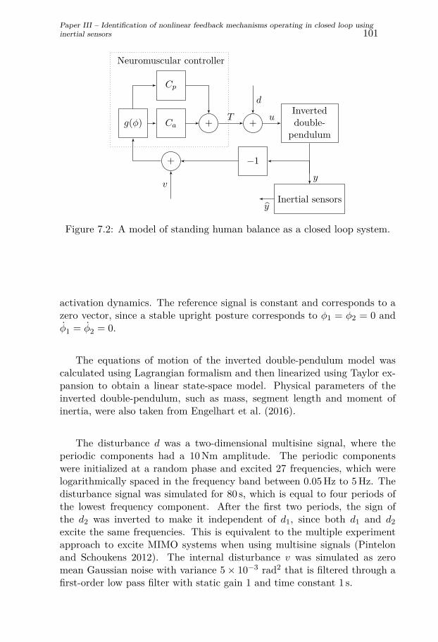
Paper III – Identification of nonlinear feedback mechanisms operating in closed loop usinginertial sensors 101
Ca + +T
dInverteddouble-
pendulum
u
+
Inertial sensors
y
−1
v
g(φ)
Cp
Neuromuscular controller
y
Figure 7.2: A model of standing human balance as a closed loop system.
activation dynamics. The reference signal is constant and corresponds to azero vector, since a stable upright posture corresponds to φ1 = φ2 = 0 andφ1 = φ2 = 0.
The equations of motion of the inverted double-pendulum model wascalculated using Lagrangian formalism and then linearized using Taylor ex-pansion to obtain a linear state-space model. Physical parameters of theinverted double-pendulum, such as mass, segment length and moment ofinertia, were also taken from Engelhart et al. (2016).
The disturbance d was a two-dimensional multisine signal, where theperiodic components had a 10 Nm amplitude. The periodic componentswere initialized at a random phase and excited 27 frequencies, which werelogarithmically spaced in the frequency band between 0.05 Hz to 5 Hz. Thedisturbance signal was simulated for 80 s, which is equal to four periods ofthe lowest frequency component. After the first two periods, the sign ofthe d2 was inverted to make it independent of d1, since both d1 and d2excite the same frequencies. This is equivalent to the multiple experimentapproach to excite MIMO systems when using multisine signals (Pintelonand Schoukens 2012). The internal disturbance v was simulated as zeromean Gaussian noise with variance 5× 10⁻³ rad2 that is filtered through afirst-order low pass filter with static gain 1 and time constant 1 s.

102 7.3. Simulated standing human balance
−50 −40 −30 −20 −10 0 10 20 30 40 50−50
−40
−30
−20
−10
0
10
20
30
40
50
φ [◦]
g(φ
)
Figure 7.3: The nonlinearity g(φ) that was applied to the input of theneuromuscular controller (solid blue) compared to the line φ (dashed black).
Nonlinear controller.
A nonlinear controller was also implemented by applying the followingfunction to the input to the neuromuscular controller
g(φ) = eφ′−b
eφ′−b + 1Kφ (7.11)
φ′ = |φ|φ0b− ln(K − 1) , (7.12)
which is a logistic sigmoid function that is modulated by the function Kφ.This nonlinearity has the effect that angles below φ0 will be underestimatedby the controller and angles above φ0 will approach the line Kφ as |φ| → ∞for K ≥ 0. Small angles will be close to zero and b ≥ 0 affects how flat thefunction is for small φ. Fig.7.3 shows the nonlinearity g(φ) for K = 1.2,b = 5 and φ0 = 10◦, which was used in the simulations to obtain data froma nonlinear neuromuscular controller. This static nonlinearity models the

Paper III – Identification of nonlinear feedback mechanisms operating in closed loop usinginertial sensors 103
Table 7.1: Validation results for different models of the linear neuromuscularcontroller.
na nb nz ‖Z‖0 RMSE [Nm] FIT [%]
0 1 0 0 (8.7 6.7) (94.3 95.0)
0 2 0 0 (8.6 6.3) (94.4 95.4)
0 3 0 0 (8.6 5.7) (94.4 95.8)
0 4 0 0 (8.5 5.4) (94.4 96.1)
0 5 0 0 (8.5 5.3) (94.5 96.1)
0 6 0 0 (8.5 5.3) (94.5 96.2)
0 6 162 65 (8.4 5.3) (94.5 96.1)
Table 7.2: Validation results for different models of the nonlinear neuromus-cular controller.
na nb nz ‖Z‖0 RMSE [Nm] FIT [%]
0 1 0 0 (58.8 40.4) (59.8 67.3)
0 2 0 0 (42.1 28.8) (71.2 76.7)
0 3 0 0 (38.4 25.0) (73.7 79.7)
0 4 0 0 (37.6 24.0) (74.3 80.6)
0 5 0 0 (37.5 23.6) (74.3 80.9)
0 6 0 0 (37.7 23.5) (74.2 81.0)
0 6 162 76 (33.9 21.7) (76.8 82.4)
0 6 1250 303 (28.5 19.5) (80.5 84.2)
common hypothesis about human balance that small deviations from theequilibrium are not corrected by the neuromuscular controller.
Measurement models.
Two inertial sensors were simulated to provide the data that was usedto identify the neuromuscular controller. One sensor was attached to eachsegment of the inverted double-pendulum, and the sensors were orientedto have one axis parallel with the segment, and one axis parallel with therotation axes of the joints. Zero mean Gaussian measurement noise was

104 7.3. Simulated standing human balance
0 10 20 30 40 50 60 70 80−500
−250
0
250
500
Time [s]
Join
tto
rque
T1,
[Nm
]
0 10 20 30 40 50 60 70 80−500
−250
0
250
500
Time [s]
Join
tto
rque
T2,
[Nm
]
Figure 7.4: The true simulated outputs T of the nonlinear neuromuscularcontroller (blue) and the simulated output from the identified model (red)for the validation data set.
simulated with variance 1× 10⁻² m2/s4 for the accelerometer and 1× 10⁻⁵
rad2/s2 for the gyroscope. These measurements were then used to obtain anestimate of the states y =
[φ1 φ2
φ1
φ2
]>. The closed loop system of
standing human balance was implemented in Simulink (MathWorks, Inc.).The system was sampled with a sample period of Ts = 0.01 s.
We also need measurements of the joint torque T , generated by theneuromuscular controller, to be able to do identification. These are typically

Paper III – Identification of nonlinear feedback mechanisms operating in closed loop usinginertial sensors 105
not available in a realistic situation, but can be estimated from the outputof the system, so called inverse dynamics. A discrete-time state-space modelof the inverted double-pendulum is used, which has the form
y(t+ 1) = Fy(t) +Gu(t). (7.13)
Using the y obtained from the inertial sensors, the joint torque can be es-timated by solving the following optimization problem
u = arg minu
N−1∑
t=1‖Gu(t) + F y(t)− y(t+ 1)‖22
+ ‖λ(u(t+ 1)− u(t))‖22
(7.14)
T = u− d, (7.15)
where λ acts as a smoothing parameter to reduce the noise in the estimate.In our simulation λ = 0.0001 was chosen. The optimization problem (7.14)was solved using a Gauss-Newton algorithm (Wright and Nocedal 2006),with a sliding window containing 1000 samples and an overlap of 50 samplesbetween consecutive windows.
7.3.1 Results and discussion
Four different data sets were simulated, two using the linear controllerand two with the nonlinearity (7.11) applied to the controller input. Dif-ferent data sets were used for estimation and validation for the linear andnonlinear controllers and each data set contained N = 8000 data points.Results for the identified model of the simulated neuromuscular controllerare summarized in Table 7.1 for the linear controller, and Table 7.2 for thenonlinear controller.
The simulated neuromuscular controller uses only joint angle and angularvelocity information. Therefore, na = 0 was used for all estimated models,so there is no dependence on past controller outputs. The parameter nbcontrols up to how many past controller inputs that the linear model dependon, where nb = 1 means that the linear model only depend on current inputs.It can be seen that increasing nb barely improves the accuracy for the modelof the linear controller. Adding nonlinear parameters does not improve theaccuracy, even though 65 nonzero nonlinear parameters were identified. Thereason why some nonzero nonlinear parameters were found may be explainedby the internal noise process v, which is a filtered white noise process, that isnot observable by the inertial sensors. It would be interesting to investigatefurther, how the internal disturbance affects the identified model. Note alsothat the nonlinear parameters used in the identification in this example only

106 7.4. Position servo
depend on current controller inputs to keep the number of parameters low,whereas the linear predictor model depend on nb − 1 past controller inputsas well.
For the model of the nonlinear neuromuscular controller it is clear thata linear model is too restrictive, and that increasing nb only improves theaccuracy to some extent. Adding nonlinear parameters improved the ac-curacy further. As the the number of nonlinear parameters increased, lessnonzero parameters were found relative to the total number of allowed non-linear parameters. Fig. 7.4 shows the simulated output from the identifiednonlinear model with best FIT when applied to the validation data.
7.4 Position servoA position servo is a closed loop system that consists of a motor, an
angular sensor and a feedback controller, where the motor axis angle φshould follow a desired reference signal r. We define the control error ase = r − φ, and the objective of the controller is to attain e = 0. To achievethis objective the controller will generate a control signal in the form of avoltage u, which is used to drive the motor. For this example we use aDC motor which operates in the voltage range of ±2.5V. The DC motor isconnected to a flat circular disk, whose rotation angle φ is to be controlled.
The identification data collected from each experiment was
D ={(u(t), φ(t), φ(t)
)}, t = 1, . . . , N, (7.16)
where the controller output u(t) is known exactly, since we have direct accessto the implemented controller. The controller input consists of the estimatedangle φ and angular velocity
φ. Thus, the inertial sensors provide moreinformation than the controller uses. Note that the actual controller inputare measurements of φ that comes from an angular transducer built intothe experimental setup, whereas the identification data comes from inertialsensors.
The controller used in the experiments is a lead-filter, with the transferfunction
C(s) = 0.4386s+ 1.5190.8661s+ 1 . (7.17)
The controller was implemented on a computer, with a sample rate of Ts =0.025s. The difference equation for this linear discrete-time controller hasthe form of
u(t) = 0.9715u(t− 1)+ 0.5064e(t)− 0.4632e(t− 1).
(7.18)

Paper III – Identification of nonlinear feedback mechanisms operating in closed loop usinginertial sensors 107
Figure 7.5: The experimental setup for the position servo with inertialsensors attached.
A non-linear controller was also implemented, where a static non-linearityh, defined as
h(u, umin, umax) =
0, |u| < umin
u, umin ≤ |u| ≤ umaxumax, |u| > umax
, (7.19)
which is a saturation and a dead zone, was applied to the controller outputu(t) (7.18).
Three Xsens MTw wireless inertial sensors (Xsens 2017), were attachedto the circular disk and used to estimate the rotation angle and angularvelocity of the disk. The experimental setup can be seen in Fig. 7.5. Thedisturbance signal d was an additional voltage signal, which was added tothe controller output. Therefore, the actual input to the DC motor wasu + d. The disturbance was generated as a multisine signal with 9 excitedfrequencies, logarithmically spaced in the frequency band between 0.2 Hz to8 Hz. Each periodic component had a random initial phase and amplitude0.3 V.
7.4.1 Results and discussion
Two data sets with N = 6802 data points were collected using the linearcontroller (7.18) and with the added non-linearity (7.19) with umin = 0.02 V

108 7.5. Conclusion and future work
0 5 10 15 20 25 30 35−1
−0.5
0
0.5
Time [s]
Volta
geu
,[V
]
Figure 7.6: The true output u of the nonlinear position servo controller(blue) and the simulated output from the identified model (red) for thevalidation data set.
and umax = 0.8 V. The first half of each data set was used for estimationand the second half for validation. The constant reference signal r = 0was used for all experiments. Results for the position servo controller aresummarized in Table 7.3 for the linear controller, and Table 7.4 for thenonlinear controller.
As the true controller depends on both current and past controller inputsas well as past controller outputs, we try different values for both na andnb. The models of the linear controller were very accurate. Extending themodel to include a nonlinear part resulted in only zero-valued nonlinearparameters, which shows that the method is able to identify a parsimoniousmodel in this example.
For the models of the nonlinear controller it can be seen that linearmodels resulted in poor accuracy. Adding nonlinear parameters improvedthe model accuracy significantly. Even though as many as 3125 nonlinearparameters were allowed, only 89 were identified as nonzero, producing asimpler, sparse model. Fig. 7.6 shows the simulated output from the identi-fied nonlinear model with best FIT when applied to the validation data.
7.5 Conclusion and future work
In this paper we have investigated the properties of the LAVA method,when used to identify linear and nonlinear controllers operating in closed

Paper III – Identification of nonlinear feedback mechanisms operating in closed loop usinginertial sensors 109
Table 7.3: Validation results for different models of the linear servo control-ler.
na nb nz ‖Z‖0 RMSE [V] FIT [%]
0 1 0 0 0.1940 58.6
0 2 0 0 0.1740 62.8
1 1 0 0 0.0072 98.5
1 2 0 0 0.0067 98.6
1 2 243 0 0.0067 98.6
Table 7.4: Validation results for different models of the nonlinear servocontroller.
na nb nz ‖Z‖0 RMSE [V] FIT [%]
0 1 0 0 0.2362 53.9
0 2 0 0 0.2338 54.4
1 1 0 0 0.3411 33.4
1 2 0 0 0.3342 34.8
0 2 81 18 0.1532 70.1
0 2 625 36 0.1523 70.3
1 2 243 31 0.0626 87.8
1 2 3125 89 0.0493 90.4
loop. Two examples were provided, a simulated standing human balancescenario and a real position servo using a DC motor. Identification datawere obtained through external, inertial sensors. The LAVA method wasable to identify sparse nonlinear models that described the dynamics of thenonlinear controllers. In the case of the linear position servo controller, aparsimonious linear model was identified, even though the model allowed fornonlinear parameters. In the case of the linear simulated balance controllersome nonzero nonlinear parameters were identified, which did not improvethe accuracy of the model.
A flexible model structure is desirable in the identification of real biolo-gical feedback systems, where linear models can be too restrictive. The stud-ied method provides flexibility, yet favours the parsimonious, sparse models

110 7.5. Conclusion and future work
in identification. In a future study, we would like to apply the method toidentify a real neuromuscular controller in human balance and compare itto previously used methods.

Paper III – Identification of nonlinear feedback mechanisms operating in closed loop usinginertial sensors 111
ReferencesDay, B., M. Steiger, P. Thompson and C. Marsden (1993). ‘Effect of vision
and stance width on human body motion when standing: implicationsfor afferent control of lateral sway.’ In: The Journal of physiology 469.1,pp. 479–499.
Engelhart, D., T. A. Boonstra, R. G. K. M. Aarts, A. Schouten and H.van der Kooij (2016). ‘Comparison of closed-loop system identificationtechniques to quantify multi-joint balance control’. In: Annual Reviewsin Control 41, pp. 58–70.
Hof, A. L. (2007). ‘The equations of motion for a standing human revealthree mechanisms for balance’. In: Journal of biomechanics 40.2, pp. 451–457.
Kok, M. (2016). ‘Probabilistic modeling for sensor fusion with inertial meas-urements’. PhD thesis. Linköping University.
Ljung, L. (1999). System Identification: theory for the user. 2nd. UpperSaddle River, NJ: Prentice Hall.
Mattsson, P., D. Zachariah and P. Stoica (2018). ‘Recursive nonlinear-systemidentification using latent variables’. accepted for publication in Auto-matica.
Olsson, F., K. Halvorsen, D. Zachariah and P. Mattsson (2018). Identific-ation of nonlinear feedback mechanisms operating in closed loop usinginertial sensors. To be presented at the 18th IFAC symposium on sys-tem identification (SYSID). Stockholm, Sweden.
Pintelon, R. and J. Schoukens (2012). System Identification: A frequencydomain approach. 2nd. Hoboken, NJ: John Wiley & Sons, Inc.
Solin, A. and S. Särkkä (2014). ‘Hilbert Space Methods for Reduced-RankGaussian Process Regression’. arXiv preprint arXiv:1401.5508.
Wright, S. and J. Nocedal (2006). Numerical Optimization. 2nd. SpringerSeries in Operations Research.
Xsens (2017). MTw Awinda Wireless Motion Tracker. (Online) https://www.xsens.com/download/pdf/documentation/mtw2-awinda/MTw2-Awinda.pdf accessed December 2017.

112 References

Paper IV
TitleNon-parametric time-domain tremor quantification with smart phonefor therapy individualization
AuthorsFredrik Olsson and Alexander Medvedev
Edited version ofF. Olsson and A. Medvedev (2018). Non-parametric Time-domain Tremor Quan-tification with Smart Phone for Therapy Individualization. Submitted for publica-tion.

114
Non-parametric time-domaintremor quantification withsmart phone for therapyindividualization
Abstract
This paper deals with a low-complexity time-domain tremor quantifica-tion method for individualization of therapies in medical conditions, wheretremor is a cardinal symptom. The method produces a tremor severity es-timate based on measurements acquired from a standard sensor platform ofa smart phone during a smooth voluntary movement. The estimate is cal-culated from a data set recorded over tens of seconds but can also be usedfor unobtrusive tremor monitoring over longer time. Besides tremor amp-litude, its frequency is also evaluated over time thus providing the meansto distinguish between e.g. rest and action tremor. No analytical model isassumed for the tremor signal form. The characterization of tremor sever-ity is performed by steady-state analysis of a Markov chain, whose statescorrespond to different intervals of tremor amplitude. The utility of the pro-posed quantification approach is illustrated by clinical data obtained duringa Deep Brain Stimulation programming session. The results are comparedwith a conventional approach utilizing spectral analysis.
8.1 Introduction
Tremor is an involuntary repetitive movement observed mainly in ex-tremities but also in head and trunk. It is a cardinal symptom of neuro-logical disorders, such as Parkinson’s Disease (PD) and Essential Tremor(ET), but is also present in healthy individuals. The latter form is referredto as physiological tremor and worsens under physical or emotional stress.
115

116 8.1. Introduction
In PD and ET, both of which are currently incurable conditions, therapyis aimed at alleviating the symptoms of the disease, in particular tremor.Therefore, to characterize therapeutical effect of a medical treatment, a reli-able and objective quantification of tremor is necessary. Currently, symptomquantification in neurology is performed by medical personnel using stand-ardized rating scales. For instance, Unified Parkinson’s Disease Rating Scale(UPDRS) (The International Parkinson and Movement Disorder Society2016) takes up tremor under Part II covering motor symptoms and ratesit by an integer between zero and four, (Section 2.10). Zero rating corres-ponds to no tremor and rating four is described in UPDRS as tremor causingproblems with most or all daily activities. Apparently, the level of detailin UPDRS is adopted to ocular examination and smaller improvements ordeteriorations in the patient condition cannot be adequately captured.
The need for objective and more fine-grained quantification of tremoris motivated by individualized PD treatments. Examples of individualizedpharmacotherapies are the infusion treatment with Duodopa, where a pumpdelivers the drug in gel form to the duodenum (Nyholm 2012), and a le-vodopa microtablets treatment with a smart dispenser MyFID, (Senek etal. 2017). In both cases, the administered drug dose can be in principle ad-justed to the current state of the patient while a reliable method of symptomquantification is missing.
An attempt to use state-of-the-art tremor monitoring technology PKGR©
system from Global Kinetics for dosing of microtablets is described in Jo-hansson et al. (2018). In fact, PKGR© is designed for longitudinal tremormonitoring and applies off-line data processing which mode is not suitablein titration procedures where a drug-induced change occurs in a matter ofminutes. Another recently reported approach utilizes 3D accelerometer andgyroscope measurements during a hand pronation-supination test to capturethe dose-effect profiles of PD patients treated with levodopa, (Thomas et al.2017). The latter technique demands wearable sensors and is not unobtrus-ive as the test has to be performed each time a patient state estimate isneeded.
Another PD therapy that is in great need of individualization is DeepBrain Stimulation (DBS), where the therapeutical effect is achieved by de-livering pulsatile electrical stimulation to a certain target area of the brainvia implanted leads. The effect of DBS critically depends on the stimu-lation pulse sequence parameters that are frequency, amplitude, and dutycycle (pulse length). Since a typical DBS lead features from four to eightcontacts that also have to be suitably selected for proper stimulation, thecomplexity of the therapy individualization (usually referred to as DBS pro-gramming) is high. In contrast with the pharmacotherapies, the patient’sresponse to a change in the stimulation setting can be observed in a matter of

Paper IV – Non-parametric time-domain tremor quantification with smart phone fortherapy individualization 117
seconds. Even though model-based methods for DBS individualization arecurrently under development (Amon and Alesch 2017; Cubo et al. 2016),clinical practice is still based on a trial-and-error procedure of tuning theDBS parameters to best effect evaluated by the clinician and perceived bythe patient. Tremor is one of the targeted symptoms in individualizingDBS stimuli and lack of quantification tools effectively prevents objectivecomparison of the therapeutical effects for different stimulation parameters.
Accurate measurement of tremor is not a challenging task and can beperformed in a laboratory environment by any standard motion capturetechnique. A classical and straightforward approach in this direction is toinstruct the patient to draw over a simple geometrical form depicted on thescreen of a tablet computer or smart phone (Westin et al. 2010). The devi-ation from the predefined line is a 2D projection of the tremor movement andsuitable for direct symptom severity evaluation. Yet, the expected level ofpatient collaboration is high and can be perceived as tiring with multiple re-petitions. Further, the test situation itself can provoke performance anxietyand potentially worsen the tremor. A non-obtrusive tremor quantificationhas therefore to build on habitual and unguided voluntary movements.
Once a tremor signal as a deviation from a given voluntary movementis obtained, it has to be processed in order to evaluate tremor severity.A suitable basic technique is then to integrate absolute value of the tremorsignal and normalize it with respect to the length of the voluntary movement.However, in most practical cases, the tremor signal is not readily availablebut has to be estimated from accelerometer measurements. In fact, thevoluntary movement is not available either, while it clearly impacts themovement acceleration.
Since derivation is a linear operator and acceleration is second derivat-ive of position, one can attempt to apply signal analysis tools directly tothe measured acceleration of the patient’s limbs. This is routinely doneby assuming (broad-sense) stationarity of tremor meaning that the spectralproperties of the signal do not change in time. If, in addition, a spectraldecomposition of the voluntary movement and the tremor signal can be as-serted, power spectral analysis provides simple and effective tools for tremorquantification (Dai et al. 2015). Yet, as it is shown in Section 8.3 of this pa-per, actual accelerometer measurements of tremor exhibit time-varying amp-litude and frequency. Besides, different peak frequencies appear in differentdirections of the 3D signal, probably due to nonlinearity of the biomechan-ical system executing the translational-rotational movement (Stergiou andDecker 2011).
With the intended clinical use in mind, a tremor quantification tool hasto provide concise and coherent information to the medical personnel. Fusingmeasured sensor signals is therefore necessary and a mathematical model is

118 8.2. Data acquisition
needed to enable it. As always in engineering and science, the level of detailin such a model is defined by its final use. For tremor quantification, it canbe argued that modelling the relations between the measured signals andnot the underlying biomechanical system is sufficient because dynamicallymodifying the system behaviour is not attempted in this framework.
Finally, currently available implementation platforms for tremor quan-tification deserve to be mentioned. Dedicated devices, such as PKGR©, arepopular and attractive from a regulatory point of view, while smart watchesand smart phones are gaining on (Senova et al. 2015). The possibility of se-lecting among a number of competing software solutions on the same hard-ware platform is highly appealing to both the clinical and off-clinic end user.
The contributions of this paper stand as follows:
• A complete method for tremor quantification in time domain basedon data measured with a standard smart phone and producing tremoramplitude distribution is presented.
• Deficiencies of spectral methods of tremor quantification related totime-varying signal amplitude and frequency are demonstrated on clin-ical data.
• The proposed tremor quantification method is shown to provide abetter decision-making ground in comparing therapeutical effect ofDBS settings.
The rest of the paper is organized as follows. First, the clinical datasets utilized throughout the paper are presented. Further, spectral ana-lysis is applied to the data sets in Section 8.3 to highlight the difficultiesin tremor quantification related to signal non-stationarity and nonlinearityof the underlying biomechanical system. Further, an analytical model-freetime-domain approach to tremor signal extraction is explained step-by-stepin Section 8.4. The estimated tremor amplitude is characterized by thestationary behavior of a Markov chain designed from data in Section 8.6.The obtained results are discussed with respect to clinical and technologicalrelevance in Section 8.7 and, finally, Conclusions are drawn.
8.2 Data acquisitionThe experimental data used in the present study have also been described
and utilized in previous work (Medvedev et al. 2017). These data havebeen obtained from one PD patient with an implanted DBS system. Datawere collected during a DBS programming session at the Uppsala UniversityHospital on May 30, 2017, under ethical approval obtained from Uppsala

Paper IV – Non-parametric time-domain tremor quantification with smart phone fortherapy individualization 119
0 10 20 30 40 50 60−20
−10
0
10
20
Right Left
Time [s]
Acc
eler
atio
n[m
/s2 ]
0 10 20 30 40 50 60
−4
−2
0
2
4
Right Left
Time [s]
Ang
ular
velo
city
[rad/
s]
Figure 8.1: Raw accelerometer and gyroscope signals from the trial withDBS off. The colors denote the x- (blue), y- (green) and z-axes (red) of therespective sensor. The black solid lines indicate which data that belongs tothe movement with the right and left hands, respectively. Significant tremorwas observed visually for the left hand.
Ethical Review Board. A Samsung Galaxy S5 smart phone was used tocollect the data. Only signals from the native sensors of the phone wererecorded. Linear acceleration and angular velocity were measured by theaccelerometer and the gyroscope, respectively, with the MPU-6500 inertialsensor platform manufactured by InvenSense (InvenSense 2017). The localmagnetic field was measured by the AK09911C magnetometer manufacturedby Asahi Kasei Microdevices (Asahi Kasei Microdevices Corporation 2017).

120 8.2. Data acquisition
0 10 20 30 40 50 60−20
−10
0
10
20
Right Left
Time [s]
Acc
eler
atio
n[m
/s2 ]
0 10 20 30 40 50 60
−4
−2
0
2
4
Right Left
Time [s]
Ang
ular
velo
city
[rad/
s]
Figure 8.2: Raw accelerometer and gyroscope signals from the trial withDBS1 settings. The colors denote the x- (blue), y- (green) and z-axes (red)of the respective sensor. The black solid lines indicate which data thatbelongs to the movement with the right and left hands, respectively. Notethat here the patient performed four repetitions of the movement instead ofthree. However, only the first three cycles were used for modeling purposes.
The sample rate of all sensors was fs = 100Hz.Data were collected while the patient performed a predefined task with
the smart phone. The instructions for the task were as follows. Pick up thephone from the table, move it to the ear and put then it back to the sameposition. The patient was asked to perform this task three times with eachhand. The same procedure was repeated for three separate DBS settings:
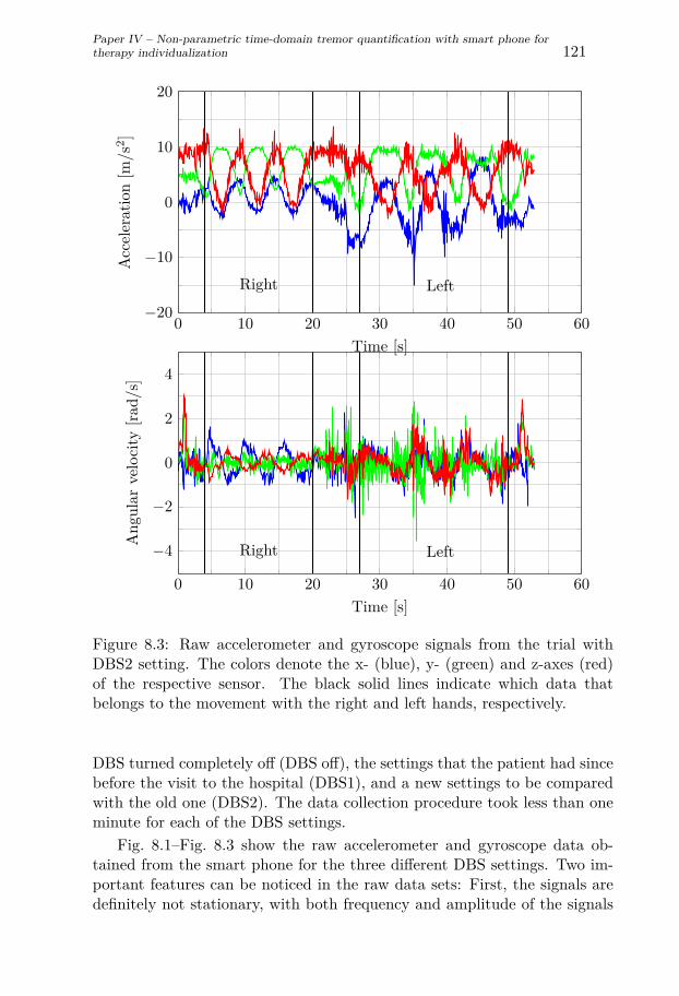
Paper IV – Non-parametric time-domain tremor quantification with smart phone fortherapy individualization 121
0 10 20 30 40 50 60−20
−10
0
10
20
Right Left
Time [s]
Acc
eler
atio
n[m
/s2 ]
0 10 20 30 40 50 60
−4
−2
0
2
4
Right Left
Time [s]
Ang
ular
velo
city
[rad/
s]
Figure 8.3: Raw accelerometer and gyroscope signals from the trial withDBS2 setting. The colors denote the x- (blue), y- (green) and z-axes (red)of the respective sensor. The black solid lines indicate which data thatbelongs to the movement with the right and left hands, respectively.
DBS turned completely off (DBS off), the settings that the patient had sincebefore the visit to the hospital (DBS1), and a new settings to be comparedwith the old one (DBS2). The data collection procedure took less than oneminute for each of the DBS settings.
Fig. 8.1–Fig. 8.3 show the raw accelerometer and gyroscope data ob-tained from the smart phone for the three different DBS settings. Two im-portant features can be noticed in the raw data sets: First, the signals aredefinitely not stationary, with both frequency and amplitude of the signals

122 8.2. Data acquisition
0 5 10 15 2010−4
10−3
10−2
10−1
100
101
102
103Φ
a(f
)[m
2 /s4 /
Hz]
Left hand
0 5 10 15 2010−4
10−3
10−2
10−1
100
101
102
103
Right hand
0 5 10 15 2010−4
10−3
10−2
10−1
100
101
102
103
Frequency, f [Hz]
Φg(f
)[ra
d2 /s2 /
Hz]
0 5 10 15 2010−4
10−3
10−2
10−1
100
101
102
103
Frequency, f [Hz]
Figure 8.4: PSD estimates of the detrended accelerometer and gyroscopesignals with DBS turned off. The colors denote the x- (blue), y- (green) andz-axes (red) of the respective sensor.
varying throughout the record time. Second, differences between Fig. 8.2and Fig. 8.3 corresponding to DBS on are difficult to discern by ocularinspection. On the contrary, the signals in Fig. 8.1 clearly confirm moreprominent tremor with DBS off. The moment when the phone reaches thehighest elevation point is also easy to recognize in each of the plots.

Paper IV – Non-parametric time-domain tremor quantification with smart phone fortherapy individualization 123
0 5 10 15 2010−4
10−3
10−2
10−1
100
101
102
103Φ
a(f
)[m
2 /s4 /
Hz]
Left hand
0 5 10 15 2010−4
10−3
10−2
10−1
100
101
102
103
Right hand
0 5 10 15 2010−4
10−3
10−2
10−1
100
101
102
103
Frequency, f [Hz]
Φg(f
)[ra
d2 /s2 /
Hz]
0 5 10 15 2010−4
10−3
10−2
10−1
100
101
102
103
Frequency, f [Hz]
Figure 8.5: PSD estimates of the detrended accelerometer and gyroscopesignals for the DBS1 setting. The colors denote the x- (blue), y- (green) andz-axes (red) of the respective sensor.
8.3 Spectral analysis methods
The most commonly encountered techniques for tremor quantificationfall within the domain of spectral analysis (Stoica and Moses 1997). Spectralanalysis generally involves estimation of the Power Spectral Density (PSD)for the signals of interest. For example, the PSD of a signal is informativeregarding what power it carries in the frequency band that is characteristicfor tremor, which typically assumed to lie between 3 to 12 Hz (Dai et al.2015).

124 8.3. Spectral analysis methods
0 5 10 15 2010−4
10−3
10−2
10−1
100
101
102
103Φ
a(f
)[m
2 /s4 /
Hz]
Left hand
0 5 10 15 2010−4
10−3
10−2
10−1
100
101
102
103
Right hand
0 5 10 15 2010−4
10−3
10−2
10−1
100
101
102
103
Frequency, f [Hz]
Φg(f
)[ra
d2 /s2 /
Hz]
0 5 10 15 2010−4
10−3
10−2
10−1
100
101
102
103
Frequency, f [Hz]
Figure 8.6: PSD estimates of the detrended accelerometer and gyroscopesignals for the DBS2 setting. The colors denote the x- (blue), y- (green) andz-axes (red) of the respective sensor.
PSD estimates Φa(f) and Φg(f) are obtained here for each axis of theaccelerometer measurements, ya, and the gyroscope measurements, yg, re-spectively, using Welch’s method with a 2s Hamming window and a 50%overlap. The accelerometer and gyroscope data are also split into separatedata sets for the right and the left hand since tremor is usually more pro-nounced on one side than on the other. The resulting PSD estimates areshown in Fig 8.4–Fig. 8.6.
To compute the signal power in a frequency band lower bounded by f1and upper bounded by f2, the PSD estimate is integrated with respect to

Paper IV – Non-parametric time-domain tremor quantification with smart phone fortherapy individualization 125
Table 8.1: The computed tremor power for all sensor axes across all trialsand for both hands. The lowest tremor powers for each hand and axis ishighlighted in boldface.
Tremor power [(Signal unit)2]Hand Trial acc-x acc-y acc-z gyr-x gyr-y gyr-z
RightDBS off 6.265 1.356 31.27 1.489 1.845 0.1928DBS1 2.218 0.3142 17.77 0.6252 0.8501 0.0761DBS2 1.418 0.2032 10.1 0.3614 0.5434 0.03608
LeftDBS off 112.9 44.2 298.3 7.246 10.5 2.551DBS1 4.044 1.196 15.87 0.7867 2.6 0.2473DBS1 16.79 4.382 18.13 1.383 5.295 1.543
frequency
Ptr =∫ f2
f1Φ(f) df. (8.1)
By selecting f1 = 3Hz and f2 = 12Hz, the contribution of tremor to thepower of a signal can then be estimated. This quantity will be referred toas the tremor power in a signal.
The dominant frequency of tremor is defined as the frequency within theinterval {f1, f2} where the PSD estimate is the highest, i.e.
fmax = arg maxf∈{f1,f2}
Φ(f). (8.2)
The dominant frequency fmax is typically used to distinguish between dif-ferent types of tremor.
The tremor power and dominant frequencies were computed for all PSDestimates and are shown in Table 8.1 and Table 8.2. The integral in (8.1)was evaluated numerically using the trapezoidal method.
8.4 Extracting the tremor signal in time domainTremor can be naturally viewed as a repetitive involuntary deviation in
position from a voluntary movement. In fact, this interpretation agrees wellwith how physicians rate tremor: The perceived amplitude of the deviationsis a measure of the symptom severity and their frequency is a secondaryparameter that helps to distinguish between different tremor types. A fun-damental difficulty in tremor quantification is then that the actual voluntarymotion cannot be measured as it is only intentional and resides in the mind

126 8.4. Extracting the tremor signal in time domain
Table 8.2: The computed dominant frequencies for all sensor axes across alltrials and for both hands.
Dominant frequency [Hz]Hand Trial acc-x acc-y acc-z gyr-x gyr-y gyr-z
RightDBS off 5.86 7.03 7.42 7.42 8.98 5.86DBS1 8.2 3.52 8.2 8.2 8.2 8.2DBS2 8.59 6.25 8.59 8.59 8.98 8.59
LeftDBS off 5.86 5.86 5.86 5.86 5.86 5.86DBS1 7.42 6.64 7.81 6.25 7.42 7.81DBS1 5.47 3.91 7.42 3.52 5.47 5.47
of the patient. Another difficulty is in the non-stationarity of tremor. Vari-ations in tremor amplitude throughout a voluntary movement are indicativeof whether the patient exhibits rest tremor or action tremor. Therefore,not only mean tremor amplitude is clinically important but the amplitudeevolution of the tremor signal as well.
This section describes how to obtain a 2D estimate of the tremor sig-nal. An estimate on a plane is used since the tremor component along thevoluntary motion is difficult to distinguish and quantify. The procedure iscovered in detail in previous work (Medvedev et al. 2017) but recapitulatedhere to facilitate readability and consists in the following four steps:
Step 1. Orientation estimation: Estimate the orientation of the sensorplatform with respect to an Earth-fixed navigation frame.
Step 2. Position estimation: Estimate the acceleration of the sensor inthe navigation frame and double integrate to estimate the position.
Step 3. Separation of tremor and voluntary movement: Estimatethe trajectory of voluntary movement and subtract it from the positionestimates.
Step 4. Planar projection and rotation: Project the 3D tremor signalonto planes perpendicular to the gradient of the voluntary movement.Then rotate all planes into the plane with zero vertical component.
8.4.1 Acceleration measurement model
The accelerometer measurements are modelled as
ya(t) = R(t)(a(t) + g) + et, (8.3)

Paper IV – Non-parametric time-domain tremor quantification with smart phone fortherapy individualization 127
where t = 1, . . . , N denotes the sample index and et is measurement noisethat is assumed to be zero-mean Gaussian. The measurements ya(t) areexpressed in the reference frame that is fixed in the accelerometer triad ofthe sensor platform, referred to as the sensor frame. The true accelerationof the sensor is denoted by a(t) and g the gravitational acceleration. Here,both a(t) and g are expressed in a earth-fixed reference frame that is referredto here as the navigation frame. The orientation of the sensor frame withrespect to the navigation frame is obtained through the rotation matrix R(t).The rotation matrices belong to the special orthogonal group R(t) ∈ SO(3),and multiplying R(t) with any vector expressed in the navigation framemaps that vector in the sensor frame.
8.4.2 Step 1. Orientation estimation
To estimate the acceleration, a(t), of the sensor platform in the navig-ation frame, the rotation matrix R(t) needs to be evaluated. An extendedKalman filter (EKF) with orientation deviation states (Kok 2016) was usedto obtain estimates R(t) of the rotation matrix. The EKF is a sensor fu-sion algorithm where the information from the gyroscope, accelerometer andmagnetometer are fused together based on a mathematical model.
When the EKF is initialized, the navigation frame is defined such that itremains fixed throughout the entire orientation estimation procedure. Theinitial accelerometer and magnetometer measurements of the sensor as itremains stationary are used to define the navigation frame. The initial ori-entation is defined as the unit matrix, R(1) = I, and the vertical directionis chosen to be aligned with the measured gravitational acceleration g. Sim-ilarly, the initial magnetometer measurements are used to define the "north"direction in the navigation frame.
The angular velocity of the sensor platform is observed through the gyro-scope. In the time update step of the EKF, the gyroscope measurementsare integrated once to update the orientation state.
Integrating gyroscope measurements over time will cause errors to ac-cumulate in the orientation estimates, something that is often referred toas integration drift. To compensate for the drift, the EKF uses the accel-erometer and magnetometer measurements to provide absolute orientationreferences. A stationary accelerometer measures g in the sensor frame, whichis an observation of the tilt angle (angle with respect to the vertical. Themagnetometer provides the heading or azimuth angle.

128 8.4. Extracting the tremor signal in time domain
8.4.3 Step 2. Position estimation
Position estimates obtained via double integration of the accelerometersignal are prone to drift. The estimated acceleration in the navigation framecontains errors due to the noise in the accelerometer measurements as wellas errors in the estimated rotation matrix. The drift phenomenon leads erroraccumulation over time and, inevitably, to the position estimates divergencefrom the true position of the sensor.
Since the predefined movement of the sensor in the experimental setupends at the same position as it starts with, it can be used to reduce thedrift. This is done by removing a linear trend from the acceleration signalthus ensuring that the position estimates return to the initial position afterthe double integration.
With R(t) obtained by the EKF, the acceleration of the sensor in thenavigation frame is estimated as
a(t) = detrend(R>(t)ya(t)− g), (8.4)
where detrend(·) is the function that removes a linear trend across all Navailable measurements for one closed cycle. A simple double integrationscheme can then be used to obtain velocity estimates, v(t), and positionestimates p(t)
v(t+ 1) = v(t) + T a(t), (8.5)
p(t+ 1) = p(t) + T v(t) + T 2
2 a(t), (8.6)
where T is the sample period and the sensor is assumed to be at rest in thebeginning of the experiment, i.e. v(1) = 0 and p(1) = 0.
8.4.4 Step 3. Separation of tremor and voluntary movement
As previously stated, a typical frequency band for tremor is 3–12Hz.Therefore, frequency components under 3Hz are assumed to belong to thevoluntary movement. To estimate the trajectory of the voluntary movement,a Savitzky-Golay filter (Savitzky and Golay 1964) with cubic polynomialsis utilized to smooth the position estimates. Other smoothing or filteringtechniques are also known to work well, as reported in Dimitrakopoulos et al.(2017). As signal processing is not necessarily performed on-line, anti-causalfiltering that does not introduce additional phase shift is feasible here.
The 3D tremor signal is then evaluated as
pt3d(t) = pv(t)− p(t), (8.7)

Paper IV – Non-parametric time-domain tremor quantification with smart phone fortherapy individualization 129
where pv(t) are the Savitzky-Golay filtered position estimates p(t). An im-portant parameter of the Savitzky-Golay filter is the window size. To obtaina good estimate of the voluntary movement, the window size should be suf-ficiently large to cover multiple periods of tremor oscillations but not solarge that it filters the trajectory of the voluntary movement. Judging fromFig. 8.1–Fig. 8.3, the period time for the voluntary movement was in therange of 3 − 6s. It has been found that a good rule of thumb for selectinga window size for the considered voluntary movement is to set it to threeperiods of the lowest tremor frequency component.
8.4.5 Step 4. Planar projection and rotation
The final step of extracting the tremor signal is to obtain a 2D projectionfor further quantification. This is done by first projecting the 3D tremorsignal onto planes that are perpendicular to the gradient of the voluntarymovement trajectory, see Fig. 8.7. Each plane is then successively rotatedinto an orientation with zero vertical component at which the 2D tremorsignal is then extracted. The procedure can be summarized by the followingequation
pt2d(t) =(R2d(t)
[pt3d(t)−
pt3d(t) · vv(t)‖vv(t)‖22
vv(t)])
1:2, (8.8)
where vv(t) is the velocity of the voluntary movement calculated as thenumerical gradient of pv(t) and ‖ · ‖2 denotes the Euclidean norm. Therotation matrix R2d(t) consists of a sequence of multiple rotation steps
R2d(t) = Ralign(q(1))Ralign(q(2)) . . . Ralign(q(t))
=t∏
k=1Ralign(q(k)),
(8.9)
where for k > 1, Ralign(q(k)) is the rotation that aligns the normal of the k:thplane with the normal of the k − 1:th plane and Ralign(q(1)) is the rotationthat rotates the first plane into the plane with zero vertical component.Here, Ralign(q(k)) is parameterized by the unit quaternion q(k), a unit vectorin R4, that is computed as
q(k) = q(k)‖q(k)‖2
, (8.10)
q(k) =[n(k − 1) · n(k)n(k − 1)× n(k)
], (8.11)
where q(k) is the non-normalized quaternion that describes the shortest arcrotation from the unit vector n(k) to the unit vector n(k− 1), · denotes the

130 8.5. Frequency estimation using extreme points of curvature
p(t)
pv(t)
vv(t)
vv(t + 1)
p(t + 1)pv(t + 1)
Figure 8.7: Projection of the 3D tremor signal onto planes perpendicular tothe gradient (velocity) of the voluntary movement.
dot product, and × denotes the cross product of two vectors. In the presentcase, the vectors n(k) correspond to the normal vectors of the planes to bealigned
n(k) =
vv(k)‖vv(k)‖2
, 1 ≤ k ≤ N[
1√2
1√2 0
]>, k = 0.
. (8.12)
An arbitrary rotation matrix R ∈ SO(3) can be parameterized by a unitquaternion q as
R(q) =
2q21 + 2q2
2 − 1 2(q2q3 + q1q4) 2(q2q4 − q1q3)2(q2q3 − q1q4) 2q2
1 + 2q23 − 1 2(q3q4 + q1q2)
2(q2q4 + q1q3) 2(q3q4 − q1q2) 2q21 + 2q2
4 − 1
(8.13)
q =[q1 q2 q3 q4
]>, (8.14)
which form yields the rotation matrices Ralign(q(k)) in (8.9).
8.5 Frequency estimation using extreme points ofcurvature
The frequency of the tremor signal can be characterized by the timingof the extreme (turning) points of the trajectory. The time between three

Paper IV – Non-parametric time-domain tremor quantification with smart phone fortherapy individualization 131
1 1.1 1.2 1.3 1.4 1.5 1.6 1.7 1.8 1.9 2
101
102
103
104
Time [s]
Cur
vatu
reκ
Figure 8.8: The curvature of a one second segment of a tremor signal withdetected extreme points, κ(τk), indicated by the red markers.
consecutive extreme points is a measure of the tremor period, or inverse ofits frequency. Extreme points can be detected in a number of ways. Anapproach identifying the extreme points of a trajectory as the local maximaof the curvature explored in Dimitrakopoulos et al. (2017) is also adoptedin this paper.
The curvature of any twice differentiable trajectory γ in an Euclideanspace can be computed as
κ =
√‖γ′‖22‖γ′′‖22 − (γ′ · γ′′)2
‖γ′‖32, (8.15)
where γ′ is the first derivative, or velocity, and γ′′ is the second derivative,or acceleration of the trajectory. In the case at hand, γ corresponds to thetremor signal and γ′, γ′′ are obtained through numeric differentiation. Sincethe tremor trajectory is a function of time, so is its curvature, i.e. κ = κ(t).

132 8.5. Frequency estimation using extreme points of curvature
0 5 10 150
0.2
0.4DBS
off
Left
0 5 10 150
0.2
0.4
Right
0 5 10 150
0.2
0.4
DBS
1
0 5 10 150
0.2
0.4
0 5 10 150
0.2
0.4
Frequency, f [Hz]
DBS
2
0 5 10 150
0.2
0.4
Frequency, f [Hz]
Figure 8.9: Normalized histograms of the frequency estimates based on thetime between extreme points κ(τk) in the curvature of the tremor signal.The red dashed lines show the means of the estimated frequencies.
Once κ(t) is computed for a particular tremor signal, the local maximaof the function are identified at the time instants τk ∈ {τ1, τ2, . . . , τL}. Asliding window of 2l+1 samples is used to identify all time instants τk. If thesample in the middle has the largest value among all samples in the window

Paper IV – Non-parametric time-domain tremor quantification with smart phone fortherapy individualization 133
it is identified as a local maxima. An example of curvature as a function oftime with detected extreme points for a tremor signal is shown in Fig. 8.8.For the tremor signal at hand l = 4 is chosen and there are at least eightsamples between three consecutive extreme points. The sampling rate of thesensors is 100Hz, so 8 samples correspond to a frequency of 12.5Hz, which isoutside of the assumed tremor band. A general rule for sensors with samplefrequency fs is to select l such that
fs2l > 12⇔ fs
24 > l. (8.16)
The frequency estimates are then computed as
fk = 1τk+2 − τk
, ∀k = 1, . . . , L− 2. (8.17)
Normalized histograms over the estimated frequencies for the tremor signalsobtained from the data in Fig. 8.1–Fig. 8.3 are depicted in Fig. 8.9.
8.6 Markov chain model of tremor severity
The tremor signal appears to exhibit variation in amplitude, directionand frequency. The tremor amplitude is what is really debilitating for apatient as it is a measure of how far the tremor drives the actual movementaway from the voluntary one. Therefore, adopting a stochastic viewpoint ontremor amplitude variation, it can be modelled as a Markov chain. A similarapproach has been applied before to model the center of pressure (COP)trajectories in human balance experiments (Hur et al. 2012; Rasku et al.2008). The movement of the COP in quiet human standing is an effect ofinvoluntary body sway similar to the involuntary movement associated withtremor. Following the approach of Hur et al. (2012), the invariant density ofa data-driven Markov chain model is utilized to assess the severity of tremor.
Markov chain models are stochastic processes that describe how a stateXt of a dynamical system evolves over time. The defining property ofMarkov chains is that the probability of transitioning to the next stateXt+1 = xt+1 only depends on the current state Xt = xt
p(Xt+1 = xt+1|Xt = xt, Xt−1 = xt−1, . . . , X1 = x1)= p(Xt+1 = xt+1|Xt = xt).
(8.18)
This property is known as the Markov property. The space of all possiblestates that the Markov chain may attain is called the state space and denotedby S, so that x1:N ∈ S. In the application at hand, the state space is defined

134 8.6. Markov chain model of tremor severity
as discrete levels of increasing symptom severity, which are determined bythe amplitudes of the tremor signal
S = {Si | di−1 ≤ ‖pt2d(t)‖2 ≤ di}, i = 1, . . . ,M, (8.19)di = ri, r ∈ R>0, (8.20)
where r is the radius of each state. Each state Si corresponds to a set ofpoints in R2 whose distance to the origin is bounded from below and aboveby the two circular disks with radii di−1 and di, respectively. Fig. 8.10illustrates part of a tremor signal trajectory evolving in the state-space.
The probability of transitioning from one state to another is encoded inthe stochastic matrix P ∈ RM×M , where each element
Pij = p(Xt+1 = Sj |Xt = Si), i, j ∈ {1, . . . ,M}, (8.21)
gives the probability of transitioning from the i:th state to the j:th state.For the tremor signal, the matrix P is determined by
Pij =∑Nt=1 1(Xt+1 = Sj)1(Xt = Si)∑N
t=1 1(Xt = Si), (8.22)
where 1(·) is the indicator function.Let the probability of the state at time t be denoted by the row vector
p(Xt) =[p(Xt = S1) . . . p(Xt = SM )
]. (8.23)
Then it follows that
p(Xt+1) = p(Xt)P. (8.24)
If a Markov chain satisfies the property
p(Xt = Sj |X1 = Si) = 1, ∀i, j ∈ {1, . . . ,M}, (8.25)
for any positive finite integer t, it is said to be irreducible and recurrent(Norris 1998). This means that, being initialized at any state X1 ∈ S andsimulated for a sufficiently long time, the Markov chain is able to reach anystate in the state-space with probability 1. If a Markov chain satisfies (8.25),then (8.24) will converge to
π = πP, (8.26)
as t → ∞. The row vector π is thus a left eigenvector of P and is oftenreferred to in the literature as the invariant or stationary distribution of theMarkov chain, given that π is scaled such that all elements sum to one.
By selecting the state radius r for the tremor signals sufficiently large,Markov chain models that satisfy (8.25) can be constructed and thus theinvariant distribution π be calculated.

Paper IV – Non-parametric time-domain tremor quantification with smart phone fortherapy individualization 135
−8 −6 −4 −2 0 2 4 6 8−8
−6
−4
−2
0
2
4
6
8
x-coordinate [mm]
y-co
ordi
nate
[mm
]
Figure 8.10: Shows a part of a tremor signal trajectory (blue) in a state-space defined as in (8.19) with M = 14 and r = 0.5mm. The black circlescorrespond to the upper bound of the radius of each state. Detected turningpoints are shown in red.
8.6.1 Tremor quantification parameters
From the obtained invariant distributions π, the following parameters toprovide different measures of tremor severity can be extracted.
Mean distance
The average distance between the actual and voluntary movement isdefined as
dmean = rM∑
i=1iπi. (8.27)

136 8.6. Markov chain model of tremor severity
A larger dmean means that the tremor amplitudes tend to be higher thusdriving the movement away from the intended voluntary trajectory.
Standard deviation distance
A measure of uncertainty in tremor amplitude defined as
dstd =
√√√√M∑
i=1(ri− dmean)2πi. (8.28)
A larger dstd indicates that the tremor amplitudes show more variation overthe data set.
95% Percentile distance
The distance from the voluntary movement that has a 95% probabilityof containing the tremor signal, defined as
d95% = rm, (8.29)
where
m = minm
subject to(
m∑
i=1πi
)≥ 95%.
(8.30)
It is a measure of how heavy the tail of the amplitude distribution is, andhow far the largest tremor amplitudes drive the movement away from theintended voluntary trajectory.
8.6.2 Results
Following the procedure described in Section 8.4, a tremor signal pt2d(t)was obtained for both hands and all three DBS settings from the data shownin Fig. 8.1–Fig. 8.3. A state-space model defined by (8.19) was used witha state radius r = 0.5mm to construct the transition probability matrixas in (8.22). This choice of state radius was sufficient for the data to sat-isfy the conditions in (8.25). Invariant distributions π have been obtainedand are plotted with respect to the respective upper state boundaries di inFig. 8.11. The tremor quantification parameters described in Section 8.6.1were computed for every π, see Table 8.3.

Paper IV – Non-parametric time-domain tremor quantification with smart phone fortherapy individualization 137
0 2 4 6 8 10 120
0.1
0.2
0.3
0.4Pr
obab
ilityπ
Right hand
DBS offDBS1DBS2
0 2 4 6 8 10 120
0.1
0.2
0.3
0.4
Tremor amplitude [mm]
Prob
abilityπ
Left hand
DBS offDBS1DBS2
Figure 8.11: Shows the invariant distributions π computed for the differenttremor signals. Each tick on the curves correspond to a specific state Si andthe associated amplitudes are the upper bounding radius of the respectivestate.
8.7 Discussion
The present study compares different ways to quantify tremor. Spectralanalysis was used to estimate the tremor power contained in the raw acceler-ometer and gyroscope measurements and identify the dominant frequencies.The results summarized in Table 8.1 show that the lowest tremor power

138 8.7. Discussion
Table 8.3: Tremor parameters extracted from invariant distributions shownin Fig. 8.11. The smallest value for each hand is highlighted in boldface.
Trial Hand dmean [mm] dstd [mm] d95% [mm]
RightDBS off 2.3 1.4 4.5DBS1 1.5 0.9 4DBS2 1.6 1.0 3.5
LeftDBS off 3.7 2.3 8DBS1 2.1 1.4 6.5DBS2 2.7 1.7 6.5
across all sensor axes was obtained with the DBS2 setting for the right handand with the DBS1 setting for the left hand. It can also be seen in Table 8.2that the dominant frequencies vary from axis to axis, except for the datacollected from the left hand with DBS off, which case yielded, typically forParkinsonian tremor, a dominant frequency of fmax = 5.86Hz. It was alsofor DBS off that the largest tremor power among all axes was observed.
There is no doubt that it is possible to detect Parkinsonian tremor bymeans of the spectral analysis method. However, comparing the therapeut-ical effect of the stimulation settings DBS1 and DBS2 based on the samemethod is more difficult. Given the results of this study, a more natural andpromising way to quantify tremor is by evaluating the deviation in positionfrom a voluntary movement. This is similar to how physicians currently viewtremor when assessing its severity. Section 8.4 describes a way to extract arelevant tremor signal from the accelerometer, gyroscope and magnetometermeasurements collected from a smart phone.
In the obtained tremor signals, a time-varying behaviour of the tremoramplitudes and frequencies is observed. This effectively compromises theaccuracy of severity estimates calculated through spectral analysis, wheresignal stationarity is assumed. While the tremor frequency is relevant tothe problem of tremor classification, the tremor amplitude is the actualdebilitating aspect and has to be rated in order to quantify the symptomseverity.
The Markov chain model that is constructed using the tremor signals isa probabilistic model of tremor amplitude variation build for a particularsnapshot of the data. The calculated invariant distribution π characterizesthe asymptotic behavior of the Markov chain, i.e. it shows what the statedistributions would be if the chain were simulated indefinitely long. This ap-parently in conflict with the non-stationary nature of tremor as it assumes

Paper IV – Non-parametric time-domain tremor quantification with smart phone fortherapy individualization 139
that the behavior captured by the Markov chain model persists in time.Therefore, the invariant distribution π has to be seen a stationary charac-teristics of a dynamical model, an abstraction that is necessary to comparethe effect of different DBS settings. A straightforward interpretation of π ishow likely it is for the observed tremor signal to drive the actual movementa certain distance away from the voluntary one.
The results presented in Fig 8.11 and Table 8.3 suggest that the tremorseverity is similar in the right hand for both the DBS1 and DBS2 settings.However, for the left hand, it appears that the DBS1 setting produces a morefavourable effect than DBS2 in terms of the mean and standard deviationin distance.
During the DBS programming session, when the data were collected,the physician eventually decided to keep using the DBS1 setting for thepatient. This decision was mostly based on the patient’s own judgmentof what was perceived to be the best setting, since it was difficult for thephysician to visually distinguish between the effects of the two DBS settingsin question. The results of this study support the decision that was madein this particular case, but more data from different patients as well as datafrom the same patient under different stimulation settings will be needed tofully evaluate the efficacy of the method. Due to limited data at hand, thisfell outside the scope of the present paper.
Since the proposed method is based on objective measurements, it servesas a tool for physicians in individualizing therapies that aim at alleviatingtremor. Being implemented on a conventional smart phone equipped witha standard sensor platform, it is also unobtrusive, inexpensive, and highlyflexible in use. Data collection may be performed essentially anywhere andincorporated in the regular day-to-day phone usage. For example, the move-ment used when collecting data for this study is similar to answering ormaking a phone call and can be easily recognized by an app.
8.8 Conclusion
A non-parametric time-domain tremor quantification method based onmeasurements collected from inertial sensors in a smart phone is studiedand compared with a conventional technique exploiting spectral analysis.
The proposed method consists of first obtaining an estimate of the volun-tary movement underlying the data set and then extracting a tremor signalas a deviation in position from voluntary movement. The tremor amplitudevariation is characterized by the stationary state distribution of a Markovchain constructed from the tremor signal. The utility of the proposed ap-proach is illustrated on patient data recorded during a DBS programming

140 8.8. Conclusion
session. The obtained tremor quantification parameters give support tothe clinical decision made by the physician during the programming sessionbased on the patient’s judgment of the DBS settings effect.
AcknowledgementsThe authors would like to thank Nils Wesslén, Dag Nyholm, and Ingela
Nygren at the Uppsala University Hostpital for the opportunity to particip-ate in a DBS programming session and their assistance in collecting data forthis study. The authors would like to thank Kjartan Halvorsen for providinguseful feedback that helped to improve the quality of the manuscript.

Paper IV – Non-parametric time-domain tremor quantification with smart phone fortherapy individualization 141
ReferencesAmon, A. and F. Alesch (2017). ‘Systems for deep brain stimulation: re-
view of technical features’. In: Journal of Neural Transmission 124.9,pp. 1083–1091.
Asahi Kasei Microdevices Corporation (Sept. 2017). 3-axis Magnetic Sensor.url: http://www.akm.com/akm/en/product/detail/0059/.
Cubo, R., M. Åström and A. Medvedev (Aug. 2016). ‘Model-based optimiz-ation of individualized deep brain stimulation therapy’. In: IEEE Designand Test 33.4. Special issue, pp. 74–78.
Dai, H., P. Zhang and T. C. Lueth (2015). ‘Quantitative assessment of Par-kinsonian tremor based on an inertial measurement unit’. In: Sensors15.10, pp. 25055–25071.
Dimitrakopoulos, K., C. Ellmer, M. Lindström and A. Medvedev (2017).‘Tremor Quantification through Event-based Movement Trajectory Mod-eling’. In: the 2017 IEEE Conference on Control Technology and Applic-ations. Kohala Coast, HA.
Hur, P., K. A. Shorter, P. G. Mehta and E. T. Hsiao-Wecksler (Apr. 2012).‘Invariant Density Analysis: Modeling and Analysis of the Postural Con-trol System Using Markov Chains’. In: IEEE Transactions on BiomedicalEngineering 59.4, pp. 1094–1100.
InvenSense (Sept. 2017). 6 Axis MotionTracking. url: http : / / www .invensense.com/products/motion-tracking/6-axis/.
Johansson, D. et al. (Jan. 2018). ‘Individualization of levodopa treatmentusing a microtablet dispenser and ambulatory accelerometry’. In: CNSNeuroscience & Therapeutics.
Kok, M. (2016). ‘Probabilistic modeling for sensor fusion with inertial meas-urements’. PhD thesis. Linköping University.
Medvedev, A., F. Olsson and T. Wigren (2017). ‘Tremor quantificationthrough data-driven nonlinear system modeling’. In: Decision and Con-trol (CDC), 2017 IEEE 56th Annual Conference on. (Melbourne, Aus-tralia). IEEE, pp. 5943–5948.
Norris, J. R. (1998). Markov chains. 2nd. Cambridge, UK: Cambridge Uni-versity Press.
Nyholm, D. (Sept. 2012). ‘Duodopa R© treatment for advanced Parkinson’sdisease: a review of efficacy and safety’. In: Parkinsonism Relat Disord18.8, pp. 916–929.
Olsson, F. and A. Medvedev (2018). Non-parametric Time-domain TremorQuantification with Smart Phone for Therapy Individualization. Submit-ted for publication.

Paper IV – Non-parametric time-domain tremor quantification with smart phone fortherapy individualization
Rasku, J., M. Juhola, T. Tossavainen, I. Pyykkö and E. Toppila (July 2008).‘Modelling stabilograms with hidden Markov models’. In: Journal ofMedical Engineering & Technology 32.4, pp. 273–283.
Savitzky, A. and M. Golay (1964). ‘Smoothing and Differentiation of Databy Simplified Least Squares Procedures’. In: Anal. Chem. 36.8, pp. 1627–1639.
Senek, M. et al. (2017). ‘Levodopa/carbidopa microtablets in Parkinson’sdisease: a study of pharmacokinetics and blinded motor assessment’. In:European Journal of Clinical Pharmacology 73.5, pp. 563–571.
Senova, S., D. Querlioz, C. Thiriez, P. Jedynak, B. Jarraya and S. Palfi(2015). ‘Using the accelerometers integrated in smartphones to evalu-ate essential tremor’. In: Stereotactic and functional neurosurgery 93.2,pp. 94–101.
Stergiou, N. and L. M. Decker (2011). ‘Human movement variability, nonlin-ear dynamics, and pathology: is there a connection?’ In: Human move-ment science 30.5, pp. 869–888.
Stoica, P. and R. L. Moses (1997). Introduction to Spectral Analysis. 1stEdition. Prentice Hall.
The International Parkinson and Movement Disorder Society (2016). MDSRating Scales. url: http://www.movementdisorders.org/MDS/Education/Rating-Scales.htm (visited on 23/11/2016).
Thomas, I., J. Westin, M. Alam, F. Bergquist, D. Nyholm, M. Senek andM. Memedi (2017). ‘A treatment-response index from wearable sensorsfor quantifying Parkinson’s disease motor states’. In: IEEE Journal ofBiomedical and Health Informatics PP.99, pp. 1–1.
Westin, J., M. Dougherty, D. Nyholm and T. Groth (2010). ‘A home en-vironment test battery for status assessment in patients with advancedParkinson’s disease’. In: Computer Methods and Programs in Biomedi-cine 98.1, pp. 27–35.

References


Recent licentiate theses from the Department of Information Technology2018-002 Tatiana Chistiakova: Ammonium Based Aeration Control in Wastewater
Treatment Plants - Modelling and Controller Design
2018-001 Kim-Anh Tran: Static Instruction Scheduling for High Performance onEnergy-Efficient Processors
2017-003 Oscar Samuelsson: Fault Detection in Water Resource Recovery Facil-ities
2017-002 Germán Ceballos: Modeling the Interactions Between Tasks and theMemory System
2017-001 Diana Yamalova: Hybrid Observers for Systems with Intrinsic Pulse-Modulated Feedback
2016-012 Peter Backeman: New Techniques for Handling Quantifiers in Booleanand First-Order Logic
2016-011 Andreas Svensson: Learning Probabilistic Models of Dynamical Phe-nomena Using Particle Filters
2016-010 Aleksandar Zeljic: Approximations and Abstractions for Reasoningabout Machine Arithmetic
2016-009 Timofey Mukha: Inflow Generation for Scale-Resolving Simulations ofTurbulent Boundary Layers
2016-008 Simon Sticko: Towards Higher Order Immersed Finite Elements for theWave Equation
2016-007 Volkan Cambazoglou: Protocol, Mobility and Adversary Models for theVerification of Security
2016-006 Anton Axelsson: Context: The Abstract Term for the Concrete
Department of Information Technology, Uppsala University, Sweden