TDA Progress Report 42-124 February 15, 1996

Modeling and Analysis of the DSS-14Antenna Control System

W. Gawronski and R. BartosCommunications Ground Systems Section

An improvement of pointing precision of the DSS-14 antenna is planned for thenear future. In order to analyze the improvement limits and to design new con-trollers, a precise model of the antenna and the servo is developed, including a finiteelement model of the antenna structure and detailed models of the hydraulic drivesand electronic parts. The DSS-14 antenna control system has two modes of opera-tion: computer mode and precision mode. The principal goal of this investigationis to develop the model of the computer mode and to evaluate its performance.The DSS-14 antenna computer model consists of the antenna structure and drivesin azimuth and elevation. For this model, the position servo loop is derived, andsimulations of the closed-loop antenna dynamics are presented. The model is sig-nificantly different from that for the 34-m beam-waveguide antennas.

I. Introduction

The DSS-14 antenna control system model consists of the antenna structure, antenna drives in azimuthand elevation, and the position servo loop. Each drive, in turn, consists of gearboxes, hydraulic servo(active and passive valves, hydraulic lines, and hydraulic motors), and electronics boards (amplifiersand filters). The DSS-14 antenna control system model was developed by R. E. Hill [1,2]. In the presentdevelopment, we obtain a more precise model that allows for accurate simulations of the antenna pointingerrors and allows simulation of the intermediate variables, such as torques, currents, wheel rates, trussstresses, etc. We incorporate the finite element structural model with free rotation in azimuth andelevation, in a manner similar to the 34-m antenna models [3–5], that involves cross-coupling effectsbetween azimuth and elevation, wind pressure on the dish, and pointing error model. The hydraulic partinvolves a recent development in modeling of the hydraulic components by R. Bartos [6–8].

The rate loop model consists of the elevation and azimuth drives and the antenna structure. Each driveconsists of three major components: the electronics boards, hydraulic system, and gearbox. A model ofeach component is derived separately, then put together, forming the drive and rate loop models. Finally,the position loop is closed to obtain the position loop model.

II. Drive Model

A block diagram of the drive model is shown in Fig. 1, where Nt is the ratio between motor rateand tachometer (pinion) rate; r, rad/s, is the rate input to the drive; i, A, is the hydraulic active valve

113

ELECTRONICBOARD

HYDRAULICSYSTEM

GEARBOX

ri TTo

θm•θm

•

θm•

θtach•

θp•

•1

Nt

Fig. 1. Block diagram of the antenna drive.

solenoid current; To and T , N·m or lb in., are the gearbox and on-axis torques, respectively; and θtach andθm, rad/s, are the pinion and motor rates, respectively. The state–space representation of the electronicboard, hydraulic system, and gearbox are derived in the following sections.

A. Electronic Board

A schematic diagram for the electronic board is shown in Fig. 2. The inputs are the rate commandr, rad/s, and the tachometer rate θtach, rad/s. The output is the solenoid valve current i. The scalingfactors, kr and kt, convert the inputs into the command voltage, vr, and tachometer voltage, vt. Thesubsystem, Gt, is the tachometer circuit: it transforms the tachometer voltage, vt, into the voltage, vto.The subsystems with the transfer functions Gr1 and Gr2 are the rate amplifier circuits: they transformthe command voltage, vr, and the tachometer voltage, vto, into the error voltage, vs. The subsystem withthe transfer function, Gs, is the valve driver amplifier circuit, with the error voltage, vs, as the input andthe valve current, i, as the output.

r

kt Gr2 GsiVsGto

Gr1krVr

+–VtsVto

Vrs

Vtθtach•

Fig. 2. Block diagram of the electronic board.

The following transfer functions of each of the four components are derived in the Appendix. Thetransfer function Gto for azimuth is

Gto = 0.151 (1)

and, for elevation, is

Gto = 0.127 (2)

The transfer functions Gr1 (from vr to vs) and Gr2 (from vto to vs) are

114

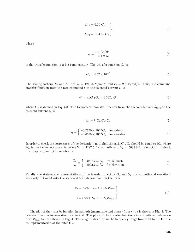
Gr1 = 6.20 Go

Gr2 = − 4.65 Go

(3)

where

Go =1 + 0.400s1 + 4.205s

(4)

is the transfer function of a lag compensator. The transfer function Gs is

Gs = 4.42× 10−5 (5)

The scaling factors, kr and kt, are kr = 1212.6 V/rad/s and kt = 2.5 V/rad/s. Thus, the commandtransfer function from the rate command r to the solenoid current is is

Gr = krGr1Gs = 0.3323 Go (6)

where Go is defined in Eq. (4). The tachometer transfer function from the tachometer rate θtach to thesolenoid current is is

Gt = ktGtoGr2Gs (7)

Gt =−0.7750× 10−4Go for azimuth−0.6525× 10−4Go for elevation

(8)

In order to check the correctness of the derivation, note that the ratio Gr/Gt should be equal to No, whereNo is the tachometer-to-axis ratio (No = 4287.5 for azimuth and No = 5083.6 for elevation). Indeed,from Eqs. (6) and (7), one obtains

GrGt

=−4287.7 = No for azimuth−5092.7 ∼= No for elevation

(9)

Finally, the state–space representations of the transfer functions Gr and Gt (for azimuth and elevation)are easily obtained with the standard Matlab command in the form

xb = Abxb +Bb1r +Bb2θtach

i = Cbx+Db1r +Db2θtach

(10)

The plot of the transfer function in azimuth (magnitude and phase) from r to i is shown in Fig. 3. Thetransfer function for elevation is identical. The plots of the transfer functions in azimuth and elevationfrom θtach to i are shown in Fig. 4. The magnitudes drop in the frequency range from 0.01 to 0.1 Hz dueto implementation of the filter Go.

115

10–3 10–2 10–1 100 101 102

101

100

10–1

FREQUENCY, Hz

CU

RR

EN

T M

AG

NIT

UD

E, A

AZIMUTH AND ELEVATION

Fig. 3. Magnitude of the electronic board transfer function from the rate input to theboard current.

10–4

10–3 10–2 10–1 100 101 10210–5

FREQUENCY, Hz

CU

RR

EN

T M

AG

NIT

UD

E, A

AZIMUTH

ELEVATION

Fig. 4. Magnitude of the electronic board transfer function from the tachometer rateinput to the board current.

10–3

B. Hydraulic System

The hydraulic servo system model was presented by R. E. Hill in [1] and [2]. Here we take a differentapproach, based on the recent investigations of hydraulic components by R. Bartos (see [6–8]). A blockdiagram of the DSS-14 hydraulic system is shown in Fig. 5. It consists of the hydraulic motor, shortingvalve, hydraulic lines A and B, passive servo valves, and active servo valves. It has two inputs, servovalve current i and motor rate θm, and one output, motor torque To. The equations for each componentare derived separately based on the work of Bartos [6–8]. Basically, these models are nonlinear ones;however, we linearize them in order to model the antenna linear regime of operation.

1. Active Servo Valve. This valve model has the input, i, A, and two outputs, qav—the flow rateout of port a, cm3/s, or in.3/s, and qbv, the flow rate out of port b, cm3/s, or in.3/s. From [6], one obtains

q·av + 2ζoωoqav + ω2oqav = ω2

okai (11a)

qbv = −qav (11b)

where ζo = 0.8 is the damping ratio, ωo = 345.6 rad/s is the valve natural frequency, and ka = 59, 200− 97, 300 cm3/s/A (23,300–38300 in.3/s/A) is the valve gain. The lower value is the Bartos estimate,while the upper value is the Hill estimate [2]. The values of the parameters are listed in Table 1.

116

pa

pb

SHORTINGVALVE

HYDRAULICLINE A

HYDRAULICLINE B

PASSIVESERVOVALVE

HYDRAULICMOTOR

ACTIVESERVOVALVE

i

θm•

qa

qb

To

θm•

pc

pa

pb

pb

pb

qb

qa

pa

pa

pspt

qbs

qas

qbpqap

qbv

qav

–

––

– –

–+

+

Fig. 5. Block diagram of the hydraulic drive.

•

•

Table 1. Parameters of the active servo valve (line A and line B).

ωo, ka, ka,Drive ζo

rad/s cm3/s/A in.3/s/A

Azimuth 0.6 to 0.8 345.56 59,200 to 97,300 23,300 to 38,300

Elevation 0.6 to 0.8 345.56 59,200 to 97,300 23,300 to 38,300

Introducing the new variable qv = qav − qbv, one obtains from Eq. (11)

q·v + 2ζoωoqv + ω2oqv = 2ω2

okai (12)

The differential variable qv and the other differential variables introduced allow one to further simplifythe analysis without loss of accuracy and to get rid of the “parasitic” variables, such as tank pressure,supply pressure, and case pressure.

2. Shorting Valve. The pressures pa and pb, kPa (lb/in.2), are the inputs to the shorting valve, andthe flows qas and qbs, cm3/s (in.3/s), are its output (see Fig. 5). The linearized relationship between theinputs and outputs is as follows:

qas = ks(pa − pb)

qbs = − qas

(13)

where ks is the valve gain, ks = 0.0007−0.007 cm3/s/kPa (0.0003–0.003 in.3/s/psi), both in azimuth andelevation.

117

Introducing new differential variables p = pa − pb and qs = qas − qbs, one obtains Eq. (13) in the form

qs = 2ksp (14)

3. Passive Servo Valve. This valve has four inputs: pressures pa and pb, supply pressure ps, andtank pressure pt. The last two are supplementary constant inputs that can be removed from the analysis.The valve has two outputs: flows qap and qbp. Its linearized input–output relationship is as follows:

qap = kp1(pa − ps) + kp2(pa − pt) (15a)

qbp = kp1(pb − ps) + kp2(pb − pt) (15b)

where the gains are kp1 = 0.0055 cm3/kPa (0.00233 in.3/psi) and kp2 = kp1, the supply pressure is17,240 kPa (2500 psi), and the tank pressure is 345 kPa (50 psi). These values are identical for azimuthand elevation.

Introducing qp = qap− qbp, and recalling that p = pa− pb, one obtains Eqs. (15a) and (15b) as follows:

qp = (kp1 + kp2)p = 2kpp (16)

where, for simplicity of notation, we denote kp = kp1 = kp2.

4. Hydraulic Motor. The motor is described in [8]. From Fig. 5, it follows that the motor has fourinputs and four outputs. The inputs are pressures pa and pb, case pressure pc, and motor rate θm, rad/s.The outputs are flows qa and qb, leakage to the case qc, and motor torque To, N·m (or lb in.). Following[8], one obtains the flow qa from Eq. (59) of [8]:

qa = qa1 + qa2 + qa3 (17)

But, from Eq. (40) of [8],

qa1 = Dθm (18)

where D = 6.3 cm3/rad (0.3836 in.3/rad) is the motor “displacement.” From Eq. (52) of [8], one obtains

qa2 =ka2

µ(pa − pc) (19)

where ka2 = from 6.35 × 10−5 to 18.3 × 10−5 cm3 (from 2.5 × 10−5 to 7.2 × 10−5 in.3) is the leakageconstant (assumed to be 10−4 cm3, or 4 × 10−5 in.3); µ = from 2.8 × 10−4 to 2.8 × 10−3 kPa s (from4× 10−5 to 4× 10−6 lb s/in.2) is the absolute fluid viscosity (assumed to be 10−4 cm3, or 4× 10−5 in.3);and pc = 221 kPa (32 psi). From Eq. (58) of [8], one obtains the leakage from port A to port B, qa3:

qa3 =ka3

µ(pa − pb) (20)

118

where ka3 is the constant of proportionality determined through experiments. It is assumed to be equalto ka2, ka3 = ka2.

Combining Eqs. (17) through (20), one obtains

qa = Dθm +ka2 + ka3

µpa −

ka3

µpb −

ka2

µpc (21)

From [8], Eq. (60), one obtains the flow rate qb:

qb = qb1 + qb2 − qa3 (22)

It follows from [8], Eq. (41), that

qb1 = −qa1 = −Dθm (23)

and from [8], Eq. (53), that

qb2 =kb2µ

(pb − pc) (24)

Combining Eqs. (22), (23), (24), and (20), one obtains

qb = −Dθ − ka3

µpa +

ka3 + kb2µ

pb −kb2µpc (25)

The motor torque To is obtained from Eq. (28) of [8] by neglecting Coulomb friction and inertia torques(the latter are included in the gearbox model):

To = Tp + Tf (26)

where Tp is the torque generated by the motor and Tf is the viscous friction torque. The linearizedEq. (10) of [8] gives the torque generated by the motor:

Tp = D(pa − pb) (27)

and from Eq. (24) of [8], one obtains the viscous friction torque:

Tf = −kvDµθ (28)

where kv = 0.0438 is a dimensionless viscous friction coefficient. Combining Eqs. (26) through (28), oneobtains

To = Dpa −Dpb − kvDµθ (29)

119

Define q = qa − qb; then from Eqs. (21) and (25), one obtains

q = 2Dθm +3ka2

µp

To = Dp− kvDµθm

(30)

The motor parameters are given in Table 2.

Table 2. Parameters of the hydraulic motor (line A and line B).

D, D, pc, pc,Drive µ, kPa s µ, lb s/in.2 kv ka2, cm3 ka2, in.3

cm3/rad in.3/rad kPa psi

Azimuth 2.8× 10−4 0.4× 10−6 25.2 1.52 0.0438 4.1× 10−4 2.5× 10−5 220 32to to to to

28× 10−4 4× 10−6 11.8× 10−4 7.2× 10−5

Elevation 2.8× 10−4 0.4× 10−6 25.2 1.52 0.0438 4.1× 10−4 2.5× 10−5 220 32to to to to

28× 10−4 4× 10−6 11.8× 10−4 7.2× 10−5

5. Hydraulic Line. There are two lines: A and B. A model for line A is developed, and the modelfor line B is similar (index “a” should be replaced with “b”). Line A has four inputs, flows qa, qav, qapv,and qasv, and a single output, pressure pa (refer to Fig. 5). From [7], one obtains the line-A model as anintegrator, with the negative feedback signs as in Fig. 5:

pa = kla(−qa + qav − qap − qas) (31a)

Similarly, the line-B model is obtained:

pb = klb(−qb + qbv − qbp − qbs) (31b)

As before, defining p = pa − pb, one obtains

p = kl(−q + qv − qp − qs) (32)

In these equations, the gains are

kl =β

vo(33)

where β is the effective bulk modulus (capacitance of the line), β = 1.29× 106 kPa (1.87× 105 psi), andvo is the total volume, vo = 27, 200 cm3 (1660 in.3), so that kl = 47.3 kPa/cm3 (113 psi/in.3). The valuesare collected in Table 3.

120

Table 3. Parameters of line A and line B.

Drive β, kPa β, psi vo, cm3 vo, in.3

Line A

Azimuth 1.29× 106 1.87× 105 27,200 1653.6Elevation 1.29× 106 1.87× 105 24,500 1498.1

Line B

Azimuth 1.29× 106 1.87× 105 27,700 1690.4Elevation 1.29× 106 1.87× 105 24,600 1499.9

6. Hydraulic System Model. The model of the hydraulic system is derived by combining itselements (active servo valve, shorting valve, passive valve, hydraulic lines, and hydraulic motors). Byintroducing the new differential variables, the block diagram in Fig. 5 is simplified to the one in Fig. 6.A detailed block diagram of the hydraulic system is shown in Fig. 7. Combining Eqs. (12), (14), (16),(32), and (30) (or, alternatively, using the block diagram in Fig. 7), and defining the new state vectorxh = [x1, x2, x3]T , with three states, x1 = qv, x2 = qv, and x3 = p, and defining the input current, i,motor rate θm, and the single-output motor torque, To, one obtains

xh = Ahxh +Bhoθm +Bhii

To = Chxh +Dhoθm +Dhi

(34a)

where

HYDRAULICLINE

HYDRAULICMOTOR

ACTIVESERVOVALVE

PASSIVEVALVE

SHORTINGVALVE

•

•– –

–+i p

p

pqs

qp

q

θm•

Fig. 6. Simplified block diagram of the hydraulic drive.

121

To

θm•θm

•

qp

qs

pp•qvqv

•• qv•

i

p

q

p

• •kl2ωoka

3ka2µ

D

–krD

–2ζωo

–ωo2

ACTIVE VALVE

SHORTINGVALVE

2ks

PASSIVEVALVE

2kp

HYDRAULIC LINES

HYDRAULIC MOTORS

2D

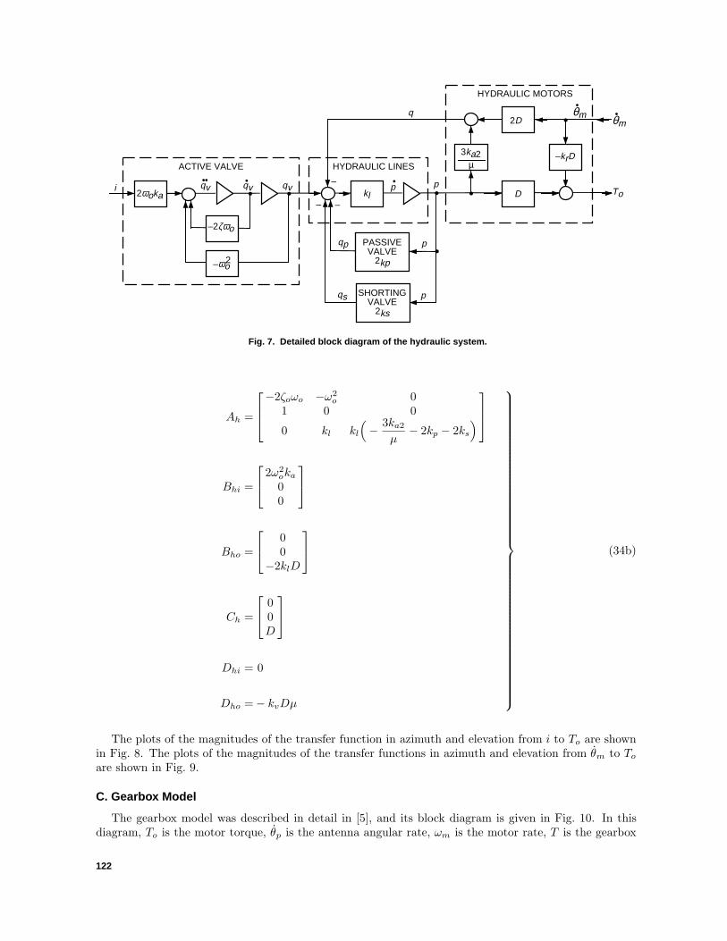
Fig. 7. Detailed block diagram of the hydraulic system.

– –

–

•

•

•

•

Ah =

−2ζoωo −ω2o 0

1 0 0

0 kl kl

(− 3ka2

µ− 2kp − 2ks

)

Bhi =

2ω2oka00

Bho =

00

−2klD

Ch =

00D

Dhi = 0

Dho =− kvDµ

(34b)

The plots of the magnitudes of the transfer function in azimuth and elevation from i to To are shownin Fig. 8. The plots of the magnitudes of the transfer functions in azimuth and elevation from θm to Toare shown in Fig. 9.

C. Gearbox Model

The gearbox model was described in detail in [5], and its block diagram is given in Fig. 10. In thisdiagram, To is the motor torque, θp is the antenna angular rate, ωm is the motor rate, T is the gearbox

122

10–2 10–1 100 101 102

FREQUENCY, Hz

AZIMUTH

ELEVATION

Fig. 8. Magnitude of the hydraulic drive transfer function from the solenoid current tothe output torque.

TO

RQ

UE

, N •

m

102

103

104

105

106

10–2 10–1 100 101 102

101

100

10–1

10–2

TO

RQ

UE

, N •

m

FREQUENCY, Hz

Fig. 9. Magnitude of the hydraulic drive transfer function from the motor rate to theoutput torque.

AZIMUTH

ELEVATION

Fig. 10. Block diagram of the gearbox.

••–

++–

θp•

To Tkg

Ns

ωm

1

N

JmS1

Nθm•

torque, Jm is the motor inertia, kg is the gearbox (output) stiffness, and N is the gearbox ratio. Thismodel has two inputs, the motor torque, To, and the wheel (pinion) angular rate, θp, and a single output,the gearbox torque, T .

The equations for this system are as follows:

123

Jmωm = To −T

N(35a)

T = kg

(θmN− θp

)(35b)

Denoting the state variables x1 = ωm and x2 = T , one obtains

x1 =−x2

NJm+ToJm

(36a)

x2 =kgx1

N− kg θp (36b)

Defining the gearbox state as xg = [x1 x2 ]T , input To and θp, and output T and ωm, one obtains thegearbox state–space representation (Ag, Bg, Cg):

xg = Agxg +Bg1To +Bg2θp

T = Cg1xg

θm =Cg2xg

(37a)

where

Ag =

0−1NJm

kgN

0

Bg1 =

[ 1Jm0

]

Bg2 =[

0−kg

]

Cg1 = [ 0 1 ]

Cg2 = [ 1 0 ]

(37b)

D. Drive Model

The drive model is obtained by combining the state–space representation of the electronic board,Eq. (10); the hydraulic system, Eq. (34); and the gearbox, Eq. (37), according to the block diagram inFig. 1. Defining the drive state vector xd = [xTb , x

Th , x

Tg ]T , we obtain the state equations

124

xd = Adxd +Bdrr +Bdtθp

T = Cdxd

(38a)

where

Ad =

Ab 0

Bb2Cg2

Nt

BhiCb Ah BhoCg2 +BhiDbeCg2

Nt

Bg1DhiCb Bg1Ch Ag +Bg1DhoCg2 +Bg1DhiDb2Cg2

Nt

Bdr =

Bb1BhiDb1

Bg1DhiDb1

Bdt =

00Bg2

Cd = [ 0 0 Cg1 ]

(38b)

The plots of the magnitudes of the transfer function in azimuth and elevation from r to T are shownin Fig. 11. The plots of the transfer functions in azimuth and elevation from θp to T are shown in Fig. 12.

III. Structure Model

The structural model is derived from the finite element model of the antenna structure with freerotations with respect to the elevation and azimuth axes. The finite element model consists of thediagonal modal mass Mm(p× p), diagonal natural frequencies matrix Ω(p× p), diagonal modal dampingmatrix Z(p× p), and modal matrix Φ(m× p), p ≤ m, which consists of p eigenvectors φi (mode shapes),i = 1, · · · , p:

Φ = [φ1, φ2, · · · , φp] (39)

Let the finite element model have m degrees of freedom, with s inputs u(t), where u is s × 1 vector,and with r outputs y(t), where y is r × 1 vector. If the input matrix is Bo(m × s), the output matrixfor displacement is Coq(r × m), and the output matrix for rates is Cov(r × m), then the input–outputrelationship is given by the following second-order differential equation:

·qm + 2ZΩqm + Ω2qm =M−1m ΦTBou

ym =CoqΦqm + CovΦqm

(40)

Define the state variable x as follows:

125

FREQUENCY, Hz

Fig. 11. Magnitude of the drive transfer function from the rate command tothe output torque.

TO

RQ

UE

, N •

m

10–2 10–1 100 101 102

1010

105

100

AZIMUTHELEVATION

FREQUENCY, Hz

Fig. 12. Magnitude of the drive transfer function from the pinion rate tothe output torque.

TO

RQ

UE

, N •

m

10–2 10–1 100 101 102

108

106

104

AZIMUTHELEVATION

xs =[x1

x2

]=[qmqm

](41)

where qm and qm are modal displacements and rates (such that q = Φqm; q is the actual displacement);then Eq. (40) can be presented as a set of first-order equations:

x1 = x2

x2 = − Ω2x1 − 2ZΩx2 +M−1m ΦBous

ys = CoqΦx1 + Covφx2

(42)

or in the following form:

xs =Asxs +Bsus

ys =Csx

(43a)

126

where

As =[

0 I−Ω2 −2ZΩ

]

Bs =[

0M−1m ΦTBo

]

Cs = [CoqΦ CovΦ ]

(43b)

is the sought state–space model in modal coordinates. In our case, us = [Ta Te ], where Ta and Teare torques at azimuth wheels and elevation pinions, respectively. The structure output consists of theelevation and azimuth encoder angles and rates, pinion angles, elevation and cross-elevation pointingerrors, and other structural variables of interest. Two outputs, θpa and θpe, the pinion rates in azimuthand elevation, are of special interest. Thus, the structural state–space equations are as follows:

xs = Asxs +BsaTa +BseTe

θpa = Cpaxs

θpe = Cpexs

y = Csx

(44)

The modal data obtained from the finite element model consist of 150 natural frequencies, ωi; modes,φi; and modal masses, mmi, i = 1, · · · , 150. Additionally, based on the measurements, the modal dampingis assumed to be 1 percent, i.e., ζi = 0.01. Based on this information, the state matrix As, as in Eq. (43b),is determined by introducing the matrix of natural frequencies, Ω = diag(ωi), and modal damping,Z = diag(ζi), i = 1, · · · , 150.

The determination of matrices Bs and Cs is presented here for the azimuth wheel torque input andthe azimuth wheel rate output. For the azimuth wheel torque input, consider the azimuth wheel of radiusra and the azimuth rail of radius Ra. Let nodes n1 be located at the contact point of the wheel and therail. The torque applied to the wheel generates the force Fa at node n1. The force is tangential to theazimuth rail. Assuming a rigid pinion, the force Fa applied to the wheel is

Fa =Tara

(45)

This force has x and y components, Fax and Fay [see Fig. 13(a)], such that

Fax = − Fa cosαa = −Tara

cosαa

Fay = Fa sinαa =Tara

sinαa

(46)

127

y

x•

αa

(b)

Va

V Vy

Vx

n1

FayFa

Fax

y

•

αa

αa

x

(a)

Fig. 13. Forces and rates at the azimuth pinion: (a) forces and (b) rates.

n1

and αa is the angle marked in this figure. Let ex and ey denote the unit vector (all but one componentare zero, and the nonzero component is equal to one), with the unit component at the location of the xand y displacement of node n1 in the finite element model. The input, F , to the finite element modelis F = Faxex + Fayey. Therefore, Bo follows from the decomposition of F , such that F = BoTa. FromEq. (46), it follows that

Bo = −exra

cosαa +eyra

sinαa (47)

Next, from Eq. (43b), it follows that the nonzero (lower) part of B, after introduction of Eq. (47), is

M−1m ΦTBo =−M−1

m

ΦT exra

cosαa +M−1m

ΦT eyra

sinαa (48a)

=−M−1m

φxra

cosαa +M−1m

φyra

sinαa (48b)

where φx and φy are vectors of modal components of x and y displacements at node n1:

φx = ΦT ex = [φx1, φx2, · · · , φx150]T

φy = ΦT ey = [φy1, φy2, · · · , φy150]T

(49)

where φxi and φyi are x and y displacements of mode i at node n1. Therefore, from Eqs. (43b) and (48b),one obtains

Bs =

[0

−M−1m

φxra

cosαa +M−1m

φyra

sinαa

](50)

The output matrix derivation is presented here for the wheel rate, θpa. The wheel rotation is

128

θpa =vara

(51)

where va is the tangential velocity of the wheel at the contact point [see Fig. 13(b)]. If vx and vy are xand y components of va, and αa is the angle marked in this figure, then

va = −vx cosαa + vy sinαa (52)

therefore,

θpa =

(−e

Tx

racosαa +

eTyra

sinαa

)q (53a)

and in modal coordinates

θpa =

(−ΦeTx

racosαa +

ΦeTyra

sinαa

)qm =

(−φ

Tx

racosαa +

φTyra

sinαa

)qm (53b)

Finally, the matrix Cs, according to Eqs. (43b) and (53b), is

Cs =[

0 −φTx

racosαa +

φTyra

sinαa

](54)

The structural model consists of m = 150 modes or 300 states. Modes not participating in systemdynamics are eliminated. Observability and controllability properties in the balanced representation areused to determine insignificant modes. The balanced representation [9] is a state–space representationwith equally controllable and observable states. The Hankel singular value is a measure of the jointcontrollability and observability of each balanced state variable. The states with small Hankel singularvalues are deleted as weakly excited and weakly observed, causing minimal modeling error.

For flexible structures with small damping and distinct poles, the modal representation is almostbalanced, c.f. [10–12], and each mode is considered for the reduction separately. For a structure withm modes, matrix Bs has 2m rows, and Cs has 2m columns. Denote bs as the last m rows of Bs, cq asthe first m columns of Cs, and cr as the last m columns of Cs. Then bsi is the ith row of bs, cqi is theith column of cq, and cri is the ith column of cr. Denote β2

si = bsibTsi, αqi = cTqicqi, and αri = cTricri. The

Hankel singular value for the ith mode is given in [11] and [12]:

γ2i =

wbiβsi√w2qiα

2qi + w2

riω2i α

2ri

4ζiω2i

(55)

where the weighting factors wbi > 0, wqi > 0, wri > 0, and i = 1, · · · ,m.

Care should be taken when determining Hankel singular values. Units should be consistent; other-wise, some inputs or outputs receive more weight in Hankel singular-value determination than necessary.Consider, for example, the azimuth encoder reading in arcseconds and the elevation encoder reading indegrees. For the same angle, the numerical reading of the azimuth encoder is 3600 larger than the eleva-tion encoder reading; hence, the elements for the azimuth output are much larger than those for elevation.

129

On the other hand, some variables need more attention than others: Pointing error and encoder readingsare the most important factors in the antenna performance; hence, their importance has to be emphasizedin mode evaluation. For consistency of units and importance of variables, the weighting factors wbi, wqi,and wri are introduced. Typically, weights are set to 1.

For each mode, the Hankel singular value is determined and used to decide on the number of modes inthe reduced structural model. For the rigid body modes, Hankel singular values tend to infinity; hence,rigid body modes are always included in the reduced model. Hankel singular values of the 150 modes ofthe antenna model are plotted in Fig. 14. The reduced order model consists of 24 modes: 2 rigid-bodymodes and 22 flexible modes.

The plots of the transfer function in azimuth and elevation (magnitude and phase) from the wheel(pinion) torque T to the axis rate θ are shown in Fig. 15. They show that the azimuth transfer functionhas low frequency resonances (about 1.2 and 2.2 Hz), which are absent in the elevation transfer function.

50 100 15000.0

0.5

1.0

1.5

HA

NK

EL

SIN

GU

LAR

VA

LUE

× 1

0–3

MODE NUMBER

Fig. 14. Hankel singular values for the antenna structure.

FREQUENCY, Hz

Fig. 15. Magnitude of the transfer function of the antenna structure: (a) direct couplingand (b) cross-coupling.

10–2 10–1 100 101 102

RA

TE

, rad

/s

10–8

10–10

10–12

AZIMUTH TORQUETO AZIMUTH RATE

ELEVATION TORQUETO ELEVATION RATE

10–5

10–10

RA

TE

, rad

/s

AZIMUTH TORQUETO ELEVATION RATE

ELEVATION TORQUETO AZIMUTH RATE

(a)

(b)

130

IV. Rate Loop Model

A rate loop block diagram is presented in Fig. 16, where Ta and Te denote the drive torques, θpa andθpe denote pinion rates, and ra and re are rate commands in azimuth and elevation, respectively. Thestate–space equations are combined from the state equations of the azimuth and elevation drives [seeEq. (38) and add subscript “a” for the azimuth drive and subscript “e” for the elevation drive] and thestructure [see Eq. (44)]. Combining them, and defining the rate loop state vector xr as xr = [xda, xde, xs],where xda and xde are azimuth and elevation drive states, one obtains the rate-loop state–space equations:

xr = Arxr +Brara +Brere

y = Crxr

θa = Caxr

θe = Cexr

(56a)

where

Ar =

Ada 0 BdtaCpa0 Ade BdteCpe

BsaCda BseCde As

Bra =

Bdra00

Bre =

0Bdre

0

Cr = [ 0 0 Cs ]

(56b)

where θa and θe are azimuth and elevation encoder readings, Cpa and Cpe are the output matrices for theazimuth and elevation pinion rates, and Ca and Ce are the output matrices for the azimuth and elevationencoders, respectively.

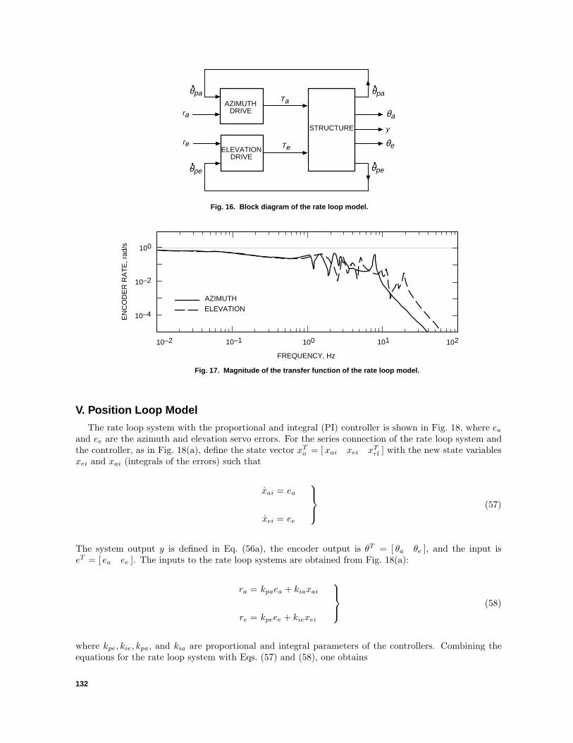
Figure 17 shows the magnitude of the transfer function from the azimuth rate input ra to the azimuthencoder rate θa (solid line) and the magnitude of the transfer function from the elevation rate input re tothe elevation encoder rate θe (dashed line). The figure shows that the required identity relationship forlow frequencies is not acquired. The magnitude of the transfer functions for frequencies less than 0.3 Hzis 0.74, below the required 1, due to inaccuracy in the model parameters (mainly in the hydraulic part).This drawback can be removed by the experimental investigation of the parameters of the hydraulicdrives, such as motors, valves, and lines. However, this inaccuracy is corrected by the position feedbackloop, as will be shown later. The high-frequency peaks in azimuth and elevation (8 Hz in azimuth and20 Hz in elevation) are the gearbox resonances.

131

STRUCTURE

AZIMUTHDRIVE

ELEVATIONDRIVE

θpe•

Taθpa• θpa

•

θpe•

Te

ra

re

y

θe

θa

Fig. 16. Block diagram of the rate loop model.

FREQUENCY, Hz

Fig. 17. Magnitude of the transfer function of the rate loop model.

10–2 10–1 100 101 102

AZIMUTHELEVATION

EN

CO

DE

R R

AT

E, r

ad/s 100

10–4

10–2

V. Position Loop Model

The rate loop system with the proportional and integral (PI) controller is shown in Fig. 18, where eaand ee are the azimuth and elevation servo errors. For the series connection of the rate loop system andthe controller, as in Fig. 18(a), define the state vector xTo = [xai xei xTrl ] with the new state variablesxei and xai (integrals of the errors) such that

xai = ea

xei = ee

(57)

The system output y is defined in Eq. (56a), the encoder output is θT = [ θa θe ], and the input iseT = [ ea ee ]. The inputs to the rate loop systems are obtained from Fig. 18(a):

ra = kpaea + kiaxai

re = kpeee + kiexei

(58)

where kpe, kie, kpa, and kia are proportional and integral parameters of the controllers. Combining theequations for the rate loop system with Eqs. (57) and (58), one obtains

132

RATELOOP

AZIMUTH PI

kpa +kias

ea

ee

ra

re

θayθe

(a)

ELEVATION PI

kpe +kies

AZIMUTH PI

kpa +kias

ELEVATION PI

kpe +kies

ea

ee

ra

rey

(b)

ca

ce +

+

RATELOOP

–

–

Fig. 18. Position loop: (a) open and (b) closed.

θe

θa

xo = Aoxo +Boe

θ = Coxo

y = Cxo

(59a)

where

Ao =

0 0 00 0 0

kiaBra kieBre Ar

Bo =

I 00 I

kpaBra kpeBre

Co =[

0 0 Ca0 0 Ce

]

C = [ 0 0 Cr ]

(59b)

For the closed-loop system [see Fig. 18(b)],

e = c− θ (60)

where cT = [ca ce] is a command signal in azimuth, ca, and in elevation, ce. Introducing Eq. (60) toEq. (59), one obtains

xcl = Aclxcl +Boc

y = Cxcl

(61a)

where

133

Acl = Ao −BoCo (61b)

The simulations shown in Figs. 19 through 22 have two sets of assumptions: (1) a proportional gainof 1 in azimuth and elevation and an integral gain of 0.3 and (2) a proportional gain of 0.7 in azimuthand elevation and an integral gain of 0.2. The closed-loop transfer functions from azimuth commandto azimuth encoder are shown in Fig. 19(a), and those from elevation command to elevation encoderare shown in Fig. 19(b). They show a bandwidth of 0.1 Hz. The cross-coupling transfer functions fromazimuth command to elevation encoder and from elevation command to azimuth encoder are shown inFig. 20. They show low-level cross-coupling. The closed-loop step responses from azimuth commandto azimuth encoder are shown in Fig. 21(a), and those from elevation command to elevation encoderare shown in Fig. 21(b). They show a 20- to 30-percent overshoot and a 7- to 9-s settling time. Thecross-coupling from azimuth step command to elevation encoder and from elevation step command toazimuth encoder is shown in Fig. 22. The cross-coupling is of the order 10−3.

10210110010–110–2

FREQUENCY, Hz

10–7

10–6

10–5

10–4

10–3

10–2

10–1

100

101

AZ

IMU

TH

EN

CO

DE

R A

NG

LE, d

eg

kp = 0.7, ki = 0.2kp = 1.0, ki = 0.3

(a)

kp = 0.7, ki = 0.2kp = 1.0, ki = 0.3

(b)

10–7

10–6

10–5

10–4

10–3

10–2

10–1

100

101

ELE

VA

TO

N E

NC

OD

ER

AN

GLE

, deg

Fig. 19. Magnitude of the transfer function of theclosed-loop system: (a) azimuth command toazimuth encoder and (b) elevation command toelevation encoder.

134

10210110010–110–2

FREQUENCY, Hz

Fig. 20. Magnitude of the transfer function of theclosed-loop system: azimuth command toelevation encoder and elevation command toazimuth encoder.

10–12

10–10

10–8

10–6

10–4

10–2

100

ELE

VA

TO

N A

ND

AZ

IMU

TH

EN

CO

DE

RA

NG

LES

, deg

AZIMUTH TO ELEVATIONELEVATION TO AZIMUTH

kp = 0.7, ki = 0.2kp = 1.0, ki = 0.3

AZ

IMU

TH

EN

CO

DE

R A

NG

LE, d

eg

(a)

1.4

1.2

1.0

0.8

0.6

0.4

0.2

TIME, s

Fig. 21. Step responses of the closed-loopsystem: (a) azimuth command to azimuthencoder and (b) elevation command to elevationencoder.

0 1 2 3 4 5 7 8 9 106

0.0

(b)

ELE

VA

TIO

N E

NC

OD

ER

AN

GLE

, deg

1.4

1.2

1.0

0.8

0.6

0.4

0.2

0.0

kp = 0.7, ki = 0.2

kp = 1.0, ki = 0.3

135

2.0

1.5

1.0

0.5

0.0

–0.5

–1.0

–1.5

–2.00 1 2 3 4 5 6 7 8 9 10

TIME, s

ELE

VA

TIO

N A

ND

AZ

IMU

TH

EN

CO

DE

RA

NG

LES

× 1

0–3 ,

deg

AZIMUTH TOELEVATIONELEVATIONTO AZIMUTH

Fig. 22. Step responses of the closed-loopsystem: azimuth command to elevation encoderand elevation command to azimuth encoder.

VI. Wind Disturbance Simulations

Wind gust disturbances were modeled similarly to the DSS-13 antenna (see [13]) using the wind tunnelpressure distribution on the dish taken from Blaylock.1 Their time history is generated using the windDavenport spectrum (see [14] and [15]), determined for the Goldstone site. The simulations for the50 km/h wind gave the results listed in Table 4 and compared with the simulation results of the DSS-13antenna. The table shows that DSS 14 has better disturbance rejection properties (at the encoders) thanhas the DSS-13 antenna.

Table 4. Servo errors in mdeg (3 σ rms)for 50 km/h wind gusts.

Drive Front wind Side wind

Elevation, DSS 14 2.6 0.7Elevation, DSS 13 14.6 1.9Azimuth, DSS 14 0.1 2.1Azimuth, DSS 13 0.5 2.3

VII. Conclusions

An analytical model of the DSS-14 antenna has been developed. The rate loop model consists of thestructural model (derived from the finite element model), gearbox model, hydraulic servo, and electronicboxes. The position loop was closed, and the time and frequency responses were simulated. The windpointing errors of the DSS-14 antenna have been simulated. The model allows for detailed simulation ofantenna dynamics and for modifications and improvements to the antenna control system.

The simulations confirmed that the use of encoders located at drives limits the performance of theantenna (mainly by reducing its bandwidth to 0.1 Hz). The use of the master equatorial or new encoders

1 R. B. Blaylock, “Aerodynamic Coefficients for Model of a Paraboloidal Reflector Directional Antenna Proposed for aJPL Advanced Antenna System,” JPL Interoffice Memorandum CP-6 (internal document), Jet Propulsion Laboratory,Pasadena, California, 1964.

136

located close to the axes of rotation of the antenna (similarly to the 34-m antennas) would allow expansionof the bandwidth to 0.7–1.0 Hz.

The antenna model needs further improvement. First, in this model, certain parameters of the hy-draulic drive are known with rather poor accuracy, and it influences the accuracy of the antenna model.It is essential to use experimental techniques to get more precise values of the parameters. Secondly, theRF pointing errors (in elevation and cross-elevation) of the antenna should be determined in order toevaluate the precision of the antenna pointing.

Acknowledgments

The authors thank Robin Bruno and Douglas Strain for development of the finiteelement model of the antenna structure, and Farrokh Baher and Abner Bernardofor help in development of the electronic board model.

References

[1] R. E. Hill, “A New State Space Model for the NASA/JPL 70-Meter AntennaServo Controls,” The Telecommunications and Data Acquisition Progress Report42-91, July–September 1987, Jet Propulsion Laboratory, Pasadena, California,pp. 247–294, November 15, 1987.

[2] R. E. Hill, “Dynamic Models for Simulation of the 70-m Antenna Axis Servos,”The Telecommunications and Data Acquisition Progress Report 42-95, July–September 1988, Jet Propulsion Laboratory, Pasadena, California, pp. 32–50,November 15, 1988.

[3] W. Gawronski and J. A. Mellstrom, “Modeling and Simulations of theDSS-13 Antenna Control System,” The Telecommunications and Data Acqui-sition Progress Report 42-106, April–June 1991, Jet Propulsion Laboratory,Pasadena, California, pp. 205–248, August 15, 1991.

[4] W. Gawronski and J. A. Mellstrom, “Control and Dynamics of the DeepSpace Network Antennas,” Control and Dynamic Systems, vol. 63, edited byC. T. Leondes, San Diego, California: Academic Press, 1994.

[5] W. Gawronski and J. A. Mellstrom, “Elevation Control System Model of theDSS-13 Antenna,” The Telecommunications and Data Acquisition Progress Re-port 42-105, January–March 1991, Jet Propulsion Laboratory, Pasadena, Cali-fornia, pp. 83–108, May 15, 1991.

[6] R. D. Bartos, “Dynamic Modeling of the Servo Valves Incorporated in the ServoHydraulic System of the 70-Meter DSN Antennas,” The Telecommunications andData Acquisition Progress Report 42-108, October–December 1991, Jet Propul-sion Laboratory, Pasadena, California, pp. 222–234, February 15, 1992.

[7] R. D. Bartos, “Dynamic Modeling of the Fluid Transmission Lines of the DSN70-Meter Antennas by Using a Lumped Parameter Model,” The Telecommuni-cations and Data Acquisition Progress Report 42-109, January–March 1992, JetPropulsion Laboratory, Pasadena, California, pp. 162–169, May 15, 1992.

137

[8] R. D. Bartos, “Mathematical Modeling of Bent-Axis Hydraulic Piston Motors,”The Telecommunications and Data Acquisition Progress Report 42-111, July–September 1992, Jet Propulsion Laboratory, Pasadena, California, pp. 224–235,November 15, 1992.

[9] B. C. Moore, “Principal Component Analysis in Linear Systems, Controllabil-ity, Observability and Model Reduction,” IEEE Trans. Autom. Control, vol. 26,pp. 17–32, 1981.

[10] A. Jonckheere, “Principal Component Analysis of Flexible Systems—Open LoopCase,” IEEE Trans. Autom. Control, vol. 27, pp. 1095–1097, 1984.

[11] W. Gawronski and J. N. Juang, “Model Reduction for Flexible Structures,”Control and Dynamic Systems, vol. 36, edited by C. T. Leondes, San Diego,California: Academic Press, pp. 143–222, 1990.

[12] W. Gawronski, Balanced Control of Flexible Structures, London: Springer, 1996.

[13] W. Gawronski, B Bienkiewicz, and R. E. Hill, “Wind-Induced Dynamics of aDeep Space Network Antenna,” Journal of Sound and Vibration, vol. 174, no. 5,1994.

[14] A. G. Davenport, “The Spectrum of Horizontal Gustiness Near the Ground inHigh Winds,” Journal of Royal Meteorol. Society, vol. 87, pp. 194–211, 1961.

[15] E. Simiu and R. H. Scanlan, Wind Effects on Structures, New York: Wiley, 1978.

Appendix

Transfer Function Derivation

Each component of the electronics board is composed of operational amplifiers (opamps), resistors,and capacitors. The basic configuration of an inverting opamp circuit is shown in Fig. A-1. The “+”terminal of the opamp is grounded; thus, the “−” terminal voltage is zero, called a virtual ground. Inthis situation, the currents i1 and i2 flowing through impedances Z1 and Z2 are equal to

i1 =vinZ1

i2 =voutZ2

(A-1)

and their sum is zero; that is, i1 = −i2. Introducing them to Eq. (A-1) gives

vout = −kvin (A-2a)

where

k =Z2

Z1(A-2b)

138

Z2

Z1Vin

i1

i2

v = 0 Vout–

+• • •

Fig. A-1. Opamp circuit.

I. Transfer Function GtoA schematic for the transfer function Gto is shown in Fig. A-2(a), where the notation and the value

of each element were taken from JPL Drawing 9479871D.2 This schematic can be simplified to the oneshown in Fig. A-2(b). In this figure,

Rs =(R−1

56 +R−157 +R−1

58 +R−159

)−1+R62 = 49.5 kΩ (A-3a)

where R56 = R57 = R58 = R59 = 100 kΩ, and R62 = 24.5 kΩ; thus, Rs = 49.5 kΩ. The component Z1 is

Z1 = R63 +R64

1 +R64C40s∼= R63 +R64 = 91.1 kΩ (A-3b)

where R63 = 40 kΩ, R64 = 51.1 kΩ, and C40 = 0.15 µF. The time constant R64C40 = 0.0077 s is small,thus neglected. Denote Rmta = 9.7 kΩ and Rmte = 7.8 kΩ the motor resistances in azimuth and elevation,respectively, and C41 = 0.15 µF. Then, the component Z2 for the azimuth drive is as follows:

Z2 =Rmta

1 +RmtaC41s∼= Rmta = 9.7 kΩ (A-4a)

and for the elevation drive,

Z2 =Rmte

1 +RmteC41s∼= Rmte = 7.8 kΩ (A-4b)

The time constants RmtaC41 = 0.0015 s and RmteC41 = 0.0012 s are of the order 10−3 s, thus consideredsmall, and neglected.

The transfer function Gto for azimuth is

Gto =Rp

Rs +Rp=

880049, 500 + 8800

= 0.151 (A-5a)

and for elevation, it is

2 JPL Drawing 9479871D (internal document), Jet Propulsion Laboratory, Pasadena, California.

139

Gto =Rp

Rs +Rp=

720049, 500 + 7200

= 0.127 (A-5b)

where Rp =(Z−1

1 + Z−12

)−1= 8.8 kΩ in azimuth and 7.2 kΩ in elevation, while Rs = 49.5 kΩ.

Vt Vto

(b)

Rs° •

Z1

•

Z2

°R57

R58

R59

Vt

R56

R62

R63

R64 C40C41 Rmt

Vto

(a)

• •° •

•

• • °

Fig. A-2. Schematic for the transfer function Gto: (a) full and (b) simplified.

II. Transfer Functions Gr1 and Gr2The transfer functions Gr1 and Gr2 are determined simultaneously. Their schematic is given in

Fig. A-3(a), the parameters parameters of which are

R15 = 750 kΩ

R50 = 100 kΩ

R51 = 12.1 kΩ

R52 = 442 kΩ

R53 = 442 kΩ

R65 = 909 kΩ

R66 = 90.9 kΩ

C31 = 1 µF

C42 = 0.1 µF

(A-6)

The schematic from Fig. A-3(a) can be transformed to the form shown in Fig. A-3(b). The value of Z3

is as follows:

Z3 = R66 +R65

1 +R65C42s∼= R66 +R65 = 106 kΩ (A-7)

140

In this variable, the small time constant R65C42 = 0.0909 s was ignored.

The value Z4 is obtained as

Z4 = R53 +Ro

1 +RoC31s= 4.65× 106 1 + 0.400s

1 + 4.205s(A-8)

where Ro = (R50 +R52 +R50R52)/R51 = 4205 kΩ.

Having determined Z3 and Z4, the transfer functions Gr1 (from vr to vs) and Gr2 (from vto to vs) areobtained:

Gr1 =Z4

R15= 6.20 Go

Gr2 =− Z4

Z3= −4.65 Go

(A-9)

where

Go =1 + 0.400s1 + 4.205s

(A-10)

is the transfer function of a lag compensator.

°R15

(b)

°–

+

•

Z3

Z4 •

•Vs

Vto°

Vr

•

R15

°

°

•

• • •

•

(a)

R65

R52 R50

R66

R51

R53Vr

C31

C42

–

+°

Vto

Z3

• •

•Z4

Vs

Fig. A-3. Schematic for the transfer functions Gr1 and Gr2: (a) full and (b) simplified.

III. Transfer Function GsThe transfer function Gs is determined from the schematic in Fig. A-4(a), and is shown in compact

form in Fig. A-4(b). For this schematic, R13 = 100 kΩ, R36 = 10 kΩ, R43 = 24.9 kΩ, and C18 = 0.1 µF;therefore, one obtains

Z5 =R36

1 +R36C18s∼= R36 = 10 kΩ (A-11)

where R36C18 = 0.0015 s ∼= 0. Since v1 = vsZ5/R43, and is = v1(Z−15 +R−1), thus,

141

Gs =isvs

=R13 + Z5

R13R43= 4.42× 10−5 (A-12)

(a)

–

+°

VsR45

C18

R36 •

R13

V1 is

•

(b)

–

+°

R43 •

Z5

•

R13

V1 is

Fig. A-4. Schematic for the transfer function Gs: (a) full and (b) simplified.

142