
MODELING AND ANALYSIS OF CAL POLY MICROGRID A Thesis ...
184
MODELING AND ANALYSIS OF CAL POLY MICROGRID A Thesis presented to the Faculty of California Polytechnic State University, San Luis Obispo In Partial Fulfillment of the Requirements for the Degree Master of Science in Electrical Engineering by Matthew Albert Guevara April 2018
Transcript of MODELING AND ANALYSIS OF CAL POLY MICROGRID A Thesis ...
MODELING AND ANALYSIS OF CAL POLY MICROGRID
A Thesis
presented to
the Faculty of California Polytechnic State University,
San Luis Obispo
In Partial Fulfillment
of the Requirements for the Degree
Master of Science in Electrical Engineering
by
Matthew Albert Guevara
April 2018

ii
© 2018
Matthew Albert Guevara
ALL RIGHTS RESERVED

iii
COMMITTEE MEMBERSHIP
TITLE: Modeling and Analysis of Cal Poly Microgrid
AUTHOR:
Matthew Albert Guevara
DATE SUBMITTED:
April 2018
COMMITTEE CHAIR:
Taufik, Ph.D.
Professor of Electrical Engineering
COMMITTEE MEMBER: Ahmad Nafisi, Ph.D.
Professor of Electrical Engineering
COMMITTEE MEMBER:
Ali Shaban, Ph.D.
Professor of Electrical Engineering

iv
ABSTRACT
Modeling and Analysis of Cal Poly Microgrid
Matthew Albert Guevara
Microgrids—miniature versions of the electrical grid are becoming increasingly
more popular as advancements in technologies, renewable energy mandates, and
decreased costs drive communities to adopt them. The modern microgrid has capabilities
of generating, distributing, and regulating the flow of electricity, capable of operating in
both grid-connected and islanded (disconnected) conditions. This paper utilizes ETAP
software in the analysis, simulation, and development of the Cal Poly microgrid.
Additionally, an ETAP power system protection tutorial is created to aid students
entering the power industry. Microprocessor-based relays are heavily utilized in both the
ETAP model and hardware implementation of the system. Case studies in this project
investigate electric power system load flow, short circuit, protection coordination, and
transient stability analysis of the Cal Poly microgrid.
Keywords: microgrid, power systems education, ETAP

v
ACKNOWLEDGMENTS
I would like to express my sincere gratitude to my advisor, Dr. Taufik, for his
wisdom and guidance. This thesis would not have been complete without his continual
support throughout the entire process. His selfless ability to encourage and assist his
many students is unparalleled, and we are all privileged to have been under his superb
instruction. Thank you, Dr. Taufik.
I would also like to thank my committee members, Dr. Ali Shaban and Dr.
Ahmad Nafisi for their knowledge and support. Your excellent courses have cemented
and steered my path towards the area of electric power systems, and for that I am very
grateful.
Eric Osborn deserves utmost credit in taking over the microgrid project and
moving it forwards. The success and survival of the project owes itself largely to Eric,
and I wish him all the best in his future endeavors.
I would like to express my dearest appreciation to my friends and colleagues,
especially: Kevin Hua, Eric Osborn, Grace Larson, Richard Liu, Calin Bukur, Elliott
Winicki, Alex Marette, and the rest of the Electrical Engineering Graduate Resource Lab.
Finally, I would like to thank my family—especially my parents Hector and
Hiromi Guevara. They have sacrificed immensely to provide me with what I have now,
and for that I am forever grateful.
vi
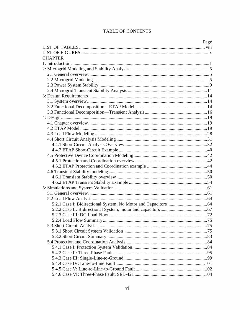
TABLE OF CONTENTS
Page LIST OF TABLES ............................................................................................................... viii LIST OF FIGURES ................................................................................................................ ix
CHAPTER
1: Introduction .......................................................................................................................... 1 2: Microgrid Modeling and Stability Analysis ....................................................................... 5
2.1 General overview ........................................................................................................... 5 2.2 Microgrid Modeling ...................................................................................................... 5 2.3 Power System Stability ................................................................................................. 9
2.4 Microgrid Transient Stability Analysis ...................................................................... 11 3: Design Requirements ......................................................................................................... 14
3.1 System overview .......................................................................................................... 14
3.2 Functional Decomposition—ETAP Model ................................................................ 14 3.3 Functional Decomposition—Transient Analysis ....................................................... 16
4: Design ................................................................................................................................. 19
4.1 Chapter overview ......................................................................................................... 19 4.2 ETAP Model ................................................................................................................ 19 4.3 Load Flow Modeling ................................................................................................... 28
4.4 Short Circuit Analysis Modeling ................................................................................ 31 4.4.1 Short Circuit Analysis Overview......................................................................... 32 4.4.2 ETAP Short-Circuit Example .............................................................................. 40
4.5 Protective Device Coordination Modeling................................................................. 42 4.5.1 Protection and Coordination overview................................................................ 42 4.5.2 ETAP Protection and Coordination example ..................................................... 44
4.6 Transient Stability modeling ....................................................................................... 50 4.6.1 Transient Stability overview ................................................................................ 50 4.6.2 ETAP Transient Stability Example ..................................................................... 54
5: Simulations and System Validation .................................................................................. 61 5.1 General overview ......................................................................................................... 61 5.2 Load Flow Analysis ..................................................................................................... 64
5.2.1 Case I: Bidirectional System, No Motor and Capacitors ................................... 64 5.2.2 Case II: Bidirectional System, motor and capacitors ......................................... 67 5.2.3 Case III: DC Load Flow ....................................................................................... 72
5.2.4 Load Flow Summary ............................................................................................ 75 5.3 Short Circuit Analysis ................................................................................................. 75
5.3.1 Short Circuit System Validation .......................................................................... 75
5.3.2 Short Circuit Summary ........................................................................................ 83 5.4 Protection and Coordination Analysis ........................................................................ 84
5.4.1 Case I: Protection System Validation.................................................................. 84
5.4.2 Case II: Three-Phase Fault ................................................................................... 95 5.4.3 Case III: Single-Line-to-Ground ......................................................................... 99 5.4.4 Case IV: Line-to-Line Fault ............................................................................... 101
5.4.5 Case V: Line-to-Line-to-Ground Fault ............................................................. 102 5.4.6 Case VI: Three-Phase Fault, SEL-421 .............................................................. 104
vii
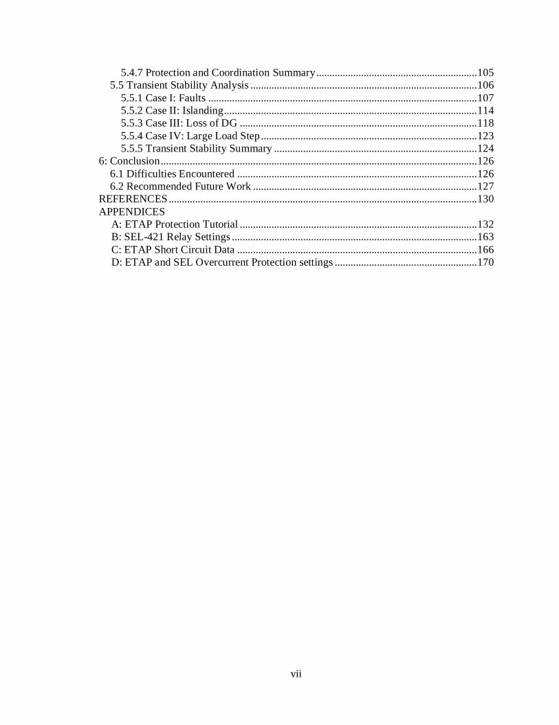
5.4.7 Protection and Coordination Summary ............................................................. 105 5.5 Transient Stability Analysis ...................................................................................... 106
5.5.1 Case I: Faults ...................................................................................................... 107 5.5.2 Case II: Islanding ................................................................................................ 114 5.5.3 Case III: Loss of DG .......................................................................................... 118
5.5.4 Case IV: Large Load Step .................................................................................. 123 5.5.5 Transient Stability Summary ............................................................................. 124
6: Conclusion ........................................................................................................................ 126
6.1 Difficulties Encountered ........................................................................................... 126 6.2 Recommended Future Work ..................................................................................... 127
REFERENCES ..................................................................................................................... 130
APPENDICES
A: ETAP Protection Tutorial .......................................................................................... 132 B: SEL-421 Relay Settings ............................................................................................. 163
C: ETAP Short Circuit Data ........................................................................................... 166 D: ETAP and SEL Overcurrent Protection settings ...................................................... 170
viii
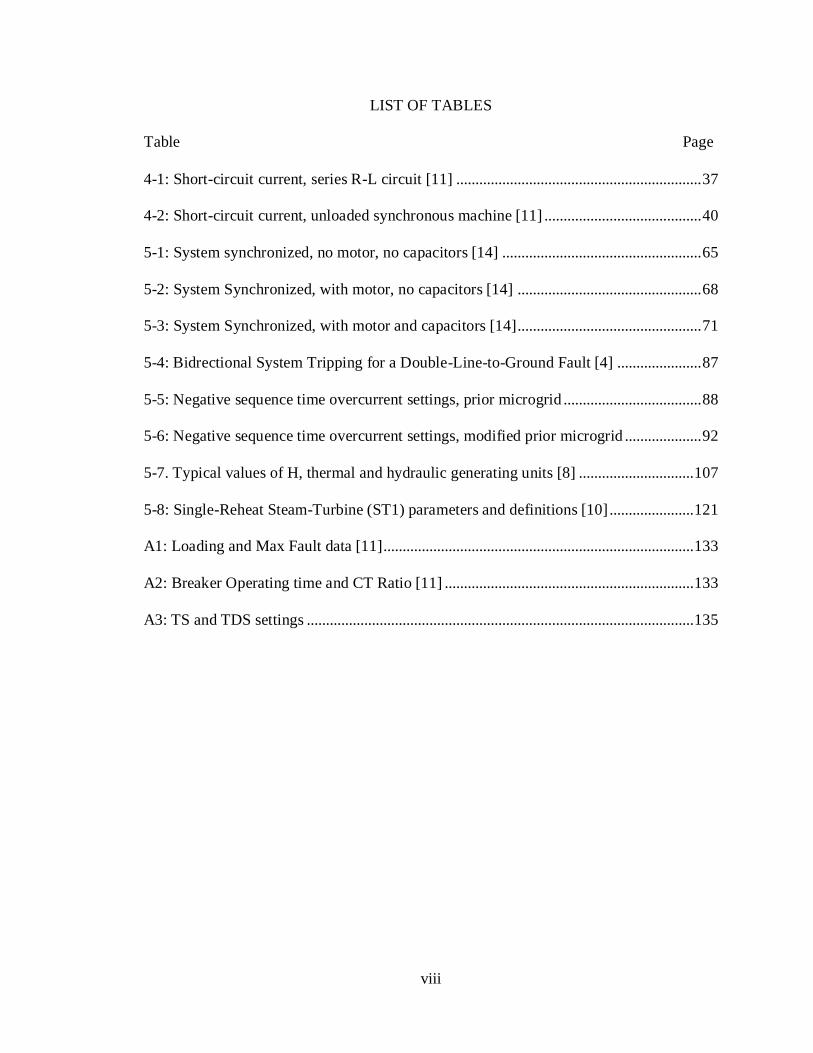
LIST OF TABLES
Table Page
4-1: Short-circuit current, series R-L circuit [11] ................................................................ 37
4-2: Short-circuit current, unloaded synchronous machine [11] ......................................... 40
5-1: System synchronized, no motor, no capacitors [14] .................................................... 65
5-2: System Synchronized, with motor, no capacitors [14] ................................................ 68
5-3: System Synchronized, with motor and capacitors [14] ................................................ 71
5-4: Bidrectional System Tripping for a Double-Line-to-Ground Fault [4] ...................... 87
5-5: Negative sequence time overcurrent settings, prior microgrid .................................... 88
5-6: Negative sequence time overcurrent settings, modified prior microgrid .................... 92
5-7. Typical values of H, thermal and hydraulic generating units [8] .............................. 107
5-8: Single-Reheat Steam-Turbine (ST1) parameters and definitions [10] ...................... 121
A1: Loading and Max Fault data [11]................................................................................. 133
A2: Breaker Operating time and CT Ratio [11] ................................................................. 133
A3: TS and TDS settings ..................................................................................................... 135

ix
LIST OF FIGURES
Figure Page
1-1: The CAISO duck chart, 2013 .......................................................................................... 3
1-2: The Opportunities Ahead: Utilities ................................................................................. 4
2-1: Bidirectional Network Single-Line Diagram [4] ............................................................ 6
2-2: Bidirectional Network Single-Line Protection Diagram [4].......................................... 7
2-3: Classification of power system stability ......................................................................... 9
2-4: Different stability issues in microgrids ......................................................................... 12
3-1: ETAP Model Block Diagram, Level 0 .......................................................................... 14
3-2: Transient Stability Block Diagram, Level 0 ................................................................. 17
3-3: Microgrid Stability Improvement .................................................................................. 18
4-1: ETAP One-Line view ..................................................................................................... 20
4-2: ETAP Microgrid PV Subsystem ................................................................................... 24
4-3: PV Array Editor .............................................................................................................. 26
4-4: Inverter Editor ................................................................................................................. 27
4-5: Load Flow Study Case Editor ........................................................................................ 29
4-6: Synchronous Generator Editor ...................................................................................... 30
4-7: Symmetrical Components of three balanced phasors [8]............................................. 33
4-8: Unbalanced voltage phasors, symmetrical components [12]....................................... 34
4-9: R-L circuit short-circuit response [11] .......................................................................... 36
4-10: Armature short circuit current with dc offset removed .............................................. 38
4-11: Extrapolation of asymmetrical AC fault current ........................................................ 41
4-12: Instrument Transformers (CTs and VTs) [11] ............................................................ 44

x
4-13: Single-line, Radial protection example [11] ............................................................... 45
4-14: ETAP Single-Line, Radial Protection example .......................................................... 46
4-15: Protective Device SQOP .............................................................................................. 47
4-16: TCC, Radial Protection example ................................................................................. 48
4-17: Bidirectional System with two sources [11] ............................................................... 49
4-18: Mechanical analogy of transient stability [11] ........................................................... 51
4-19: Synchronous Generator operation, magnetic bars [9] ................................................ 52
4-20: Three-phase synchronous machine, schematic [8] ..................................................... 53
4-21: ETAP implementation of faulted bus .......................................................................... 55
4-22: Rotor angle response, fault cleared in 0.05 seconds .................................................. 56
4-23: Electrical power output, fault cleared in 0.05 seconds............................................... 57
4-24: Unstable rotor angle response, fault cleared in 0.07 seconds .................................... 59
5-1: Utility to Bus 3, laboratory setup .................................................................................. 62
5-2: Utility to Bus 3, ETAP one line diagram ...................................................................... 62
5-3: Generators to Bus 3, laboratory setup ........................................................................... 63
5-4: Generators to Bus 3, ETAP one line diagram............................................................... 63
5-5: Load Flow, no motor and capacitors ............................................................................. 65
5-6: Load Flow, no motor and capacitors, MVAR mode .................................................... 67
5-7: ETAP Induction Motor loading conditions .................................................................. 69
5-8: Load Flow, motor energized, no capacitor ................................................................... 70
5-9: Load Flow, motor and capacitors .................................................................................. 72
5-10: DC Load Flow, DC System ......................................................................................... 73
5-11: AC Load Flow, PV generation .................................................................................... 74

xi
5-12: Three-phase short circuit test, synchronous generator ............................................... 76
5-13: ETAP, three-phase short circuit test, synchronous generator .................................... 77
5-14: SEL Oscillogram, three-phase short circuit, synchronous generator ........................ 78
5-15: Generator short circuit terminal current, three-phase fault ........................................ 79
5-16: Maximum 3-phase SC (1/2 cycle) on generator terminals ........................................ 80
5-17: Minimum 3-phase SC (30 cycle) on generator terminals .......................................... 81
5-18: Minimum 3-phase SC (30 cycle) on Bus3 .................................................................. 82
5-19: Double-Line-to-Ground Fault Bus 3, short circuit report .......................................... 83
5-20: SQOP, Double Line-to-Ground Fault, prior microgrid.............................................. 85
5-21: SQOP Report, Double Line-to-Ground, prior microgrid ........................................... 86
5-22: TCC Bidirectional Relay Coordination, prior microgrid ........................................... 90
5-23: TCC Modified Bidirectional Relay Coordination, prior microgrid .......................... 91
5-24: SQOP viewer, DLG fault improved selectivity .......................................................... 93
5-25: SEL-387E Three-Phase Fault, Bus 1, Phases A, B, C [4] ......................................... 94
5-26: ETAP, differential protection ...................................................................................... 95
5-27: SQOP, Three-Phase Fault, Motor Terminals .............................................................. 96
5-28: SQOP Events, three-phase fault motor terminals ....................................................... 97
5-29: Three-Phase Fault, Motor Terminals, TCC ................................................................ 98
5-30: SQOP, SLG, Motor Terminals .................................................................................. 100
5-31: SQOP Events, SLG, Motor Terminals ...................................................................... 100
5-32: SQOP, Line-to-Line Fault, Motor Terminals ........................................................... 101
5-33: SQOP Events, Line-to-Line Fault, Motor Terminals ............................................... 102
5-34: SQOP, Double Line-to-Ground, Motor Terminals .................................................. 103

xii
5-35: SQOP Events, Double Line-to-Ground, Motor Terminals ...................................... 103
5-36: SEL-421 test, three-phase fault Bus 2 ....................................................................... 104
5-37: SEL-421 three-phase SC test, Bus 2 ......................................................................... 105
5-38: Transient Stability, three-phase fault Bus 3 .............................................................. 108
5-39: Rotor angle response, H = 1 MW·s/MVA, 6 cycle clear ......................................... 109
5-40: Rotor angle response, H = 0.1 MW·s/MVA, 6 cycle clear ...................................... 110
5-41: Rotor angle response, H = 0.1 MW·s/MVA, 3 cycle clear ...................................... 111
5-42: Generator terminal current response, H = 0.1 MW·s/MVA, 3 cycle clear ............. 112
5-43: Generator speed response, H = 0.1 MW·s/MVA, 3 cycle clear .............................. 113
5-44: Generator speed, islanded and no load shed ............................................................. 115
5-45: Islanded, Load Shed ................................................................................................... 116
5-46: Bus 3 frequency, islanding load shed ........................................................................ 117
5-47: Generator speed, islanded and load shed .................................................................. 118
5-48: Generator speed response, loss of DG ...................................................................... 119
5-49: ST1 Governor sample data ........................................................................................ 120
5-50: Generator speed response, governor control ............................................................ 122
5-51: Large Load Step, generator frequency ...................................................................... 123
A1: Radial System [11]........................................................................................................ 132
A2: CO-8 time-delay overcurrent relay characteristics [11] ............................................. 134
A3: Max 3 phase fault for breaker CB3, Bus2 ................................................................... 135
A4: Sequence-of-Operation for Figure A3 ......................................................................... 136
A5: TCC for 3 phase fault Bus 2 ......................................................................................... 137
A6: ETAP, New Project....................................................................................................... 138

xiii
A7: ETAP, Placing AC Bus, one-line ................................................................................. 139
A8: ETAP, Bus Editor ......................................................................................................... 140
A9: ETAP, Transformer Editor, one-line ........................................................................... 141
A10: ETAP, Power Grid Editor, one-line ........................................................................... 142
A11: ETAP, Transmission Line Editor............................................................................... 144
A12: ETAP, Transmission Lines, one-line ......................................................................... 145
A13: ETAP, Static Loads .................................................................................................... 146
A14: ETAP, CT and CB ...................................................................................................... 148
A15: ETAP, complete CTs and CBs ................................................................................... 149
A16: ETAP, Overcurrent Relays ......................................................................................... 149
A17: ETAP, Current Transformer settings ......................................................................... 151
A18: ETAP, CB settings ...................................................................................................... 152
A19: ETAP, Relay OCR settings ........................................................................................ 154
A20: ETAP, Relay Output settings ..................................................................................... 155
A21: ETAP, Star mode ........................................................................................................ 157
A22: ETAP, three-phase fault, Bus2 ................................................................................... 158
A23: ETAP, Sequence-of-Operation Events, 3 phase fault............................................... 160
A24: ETAP, Create Star View............................................................................................. 161
A25: ETAP, Star TCC ......................................................................................................... 162

1
Chapter 1: Introduction
Microgrids—miniature, scaled down versions of our electrical grid are becoming
increasingly more popular as greater energy independence and extreme weather
conditions drive communities to adopt them. Conventionally, electrical power is
delivered by utilities from large power generating stations far away from end users,
transmitted across long distances, and ultimately distributed to meet the customers’
electrical needs. Advancements in technologies, decreased costs, and renewable energy
mandates are shifting the power industry away from this centralized generation model.
Instead, utilities are observing their customers not only as energy consumers but also
actively producing electrical power. The modern microgrid has capabilities of generating,
distributing, and regulating electrical power locally, utilizing distributed energy resources
(DERs) situated close to end users, including smaller power sources such as
photovoltaics (solar) and battery energy storage systems to meet the electrical demands
of the customer.
The microgrid has capabilities of operating in both grid-connected and islanded
modes—that is, connected or disconnected from the larger electrical grid, respectively.
From the customer perspective, this presents several advantages—for example, if a
power outage were to occur on the main grid due to natural disasters or electrical faults,
the microgrid can island from the grid and continue its generation and distribution of
local power. Additionally, if the microgrid requires additional generation to meet the
demands of the customer, the microgrid can reconnect with the main grid to help
supplement the customers’ energy needs.

2
From the utility perspective, transitioning the microgrid from grid-connected to
islanded conditions presents both advantages and disadvantages. A 2014 survey of over
250 utility executives concluded “…utilities said they find current interconnection
standards inadequate for safety purposes, with 54% of utilities surveyed finding that to be
the case” [1]. As microgrids continue to rise in popularity, it is imperative to study and
implement reliable and robust protection schemes as microgrids transition between grid-
connected and islanded conditions. Nonetheless, reference [2] claims “microgrids
deployment of controllable resources, such as dispatchable generation units, energy
storage, and adjustable loads, provides a quick and efficient response for changing the
microgrid generation/load, which can be utilized for supporting the grid operation.”
Maintaining the balance between power supply and load has become problematic for
utilities in recent years. Microgrids can be implemented to help control and supplement
the supply-load balance by offering storage and generation services to the main grid.
Figure 1-1 shows a net load graph by California ISO (CAISO), displaying the net
load in 2013 and forecasted future net loads [3]. The net load curves indicating years
2014-2020 can be interpreted as the net power needed to be supplied to California’s
customers from all sources of electrical power other than from renewables. The lowest
points on the curve (the belly of the “duck”) represents a point in which renewable
generation is at a maximum. Data indicates that risks of overgeneration and necessary
ramping power is increasing in future years largely due to growing solar photovoltaic
proliferation onto the grid. Currently, grid operators need to closely monitor these curves
and curtail or dispatch electrical power as needed. Microgrids can be utilized to help
“flatten” this duck curve to maintain the supply-load balance and retain grid reliability in

3
several ways. For example, when renewable penetration is at a maximum leading to risks
of overgeneration, the microgrid can store excess energy with a battery energy storage
system. As the sun begins to set after 4pm and aggregate solar penetration to the main
grid begins to decrease, microgrids can help supply the necessary ramping power needed
to meet the electrical demand of California’s customers.
Figure 1-1: The CAISO duck chart, 2013
Figure 1-2 showcases the opportunities ahead for utilities, based on a survey of
over 250 utility executives in 2014 [1]. A staggering 97% of utility executives believe

4
microgrids are a viable business opportunity within the next 10 years, with a majority of
utilities already developing or planning to operate microgrids within the same timeframe.
Figure 1-2: The Opportunities Ahead: Utilities
Microgrids are an inevitable reality—critical loads such as hospitals, data centers,
and military bases can benefit greatly from increased reliability of electric power in both
grid-connected and islanded conditions. Microgrids can also support grid operation by
storing and dispatching electrical energy as necessary. It is then imperative for future
power system engineers to expand their knowledge on fundamental power system
components such as generators, transformers, and protective relaying to account for
emerging technologies onto the grid.

5
Chapter 2: Microgrid Modeling and Stability Analysis
2.1 General overview
Future trends of developing microgrids and their integration with the utility grid
necessitate adequate tools for modeling and analysis purposes. In response for “facing a
rapidly-changing power industry, the electrical engineering department at Cal Poly San
Luis Obispo proposed Advanced Power Systems Initiatives to better prepare its students
for entering the power industry” [4]. As such, this thesis heavily builds upon the work of
[4], which developed the foundation of a microgrid laboratory at Cal Poly. To ultimately
implement a microgrid capable of islanding capabilities, it is imperative to first develop
an adequate model of the microgrid and perform a system stability analysis.
2.2 Microgrid Modeling
Figure 2-1 displays the single-line diagram of the bidirectional network designed
and implemented in a laboratory environment by previous Cal Poly students per reference
[4], which is to be utilized as the basis for the microgrid. The network represents two
different radial power systems coupled together at bus 3. In this configuration multiple
sources of power supply the loads at bus 3, which include the induction motor and static
loads. The power is supplied by three-phase AC voltages, modeled as infinite buses in
Figure 2-1, ultimately supplied by the utility. Common power system components
including power transformers and transmission lines (modeled with an inductor) are
implemented, as well as resistors to limit the total current flowing in the system.

6
Figure 2-1: Bidirectional Network Single-Line Diagram [4]
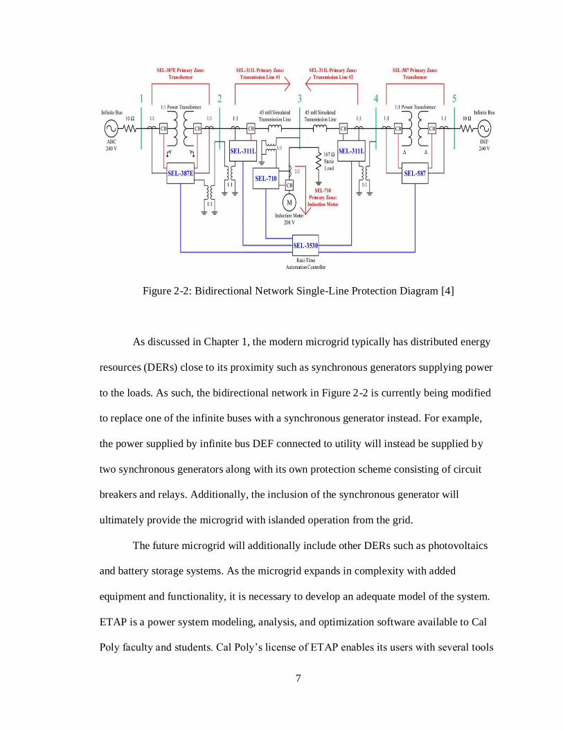
Figure 2-2 displays the protective elements within the bidirectional network as it
exists per reference [4], completed in May 2017. Schweitzer Engineering Laboratories
(SEL) microprocessor based protective relays shown in blue are constantly measuring
power system parameters such as voltages and currents, ultimately sending trip signals to
nearby circuit breakers to protect nearby components in the event of a disturbance such as
a fault. The SEL relays are programmed to trip circuit breakers on parameters such as the
type of fault (e.g. single line-to-ground, line-to-line), equipment and zone of protection
(e.g. transformer, transmission line), and protection coordination between relays (e.g.
speed and backup coordination if one relay fails to operate).
7
Figure 2-2: Bidirectional Network Single-Line Protection Diagram [4]
As discussed in Chapter 1, the modern microgrid typically has distributed energy
resources (DERs) close to its proximity such as synchronous generators supplying power
to the loads. As such, the bidirectional network in Figure 2-2 is currently being modified
to replace one of the infinite buses with a synchronous generator instead. For example,
the power supplied by infinite bus DEF connected to utility will instead be supplied by
two synchronous generators along with its own protection scheme consisting of circuit
breakers and relays. Additionally, the inclusion of the synchronous generator will
ultimately provide the microgrid with islanded operation from the grid.
The future microgrid will additionally include other DERs such as photovoltaics
and battery storage systems. As the microgrid expands in complexity with added
equipment and functionality, it is necessary to develop an adequate model of the system.
ETAP is a power system modeling, analysis, and optimization software available to Cal
Poly faculty and students. Cal Poly’s license of ETAP enables its users with several tools

8
to accurately model power systems that will ultimately benefit the microgrid project
moving forwards. For example, ETAP network analysis tools available to Cal Poly
include standard load flow, short circuit, motor acceleration, and harmonic analysis.
Protection and coordination tools include ETAP “STAR” modules to coordinate time-
current curves associated with microgrid protective elements. Transient stability tools
enable modeling of system dynamics and transients by simulating power system
disturbances.
ETAP is sufficiently capable to meet all of Cal Poly’s microgrid current modeling
and simulation needs. As the microgrid begins to implement its DERs beginning with
additional synchronous generators in Figure 2-2, synchronous generator protection and
coordination can be adequately modeled in ETAP. Future additional DERs appended to
Cal Poly’s microgrid including photovoltaics and battery storage systems can be
sufficiently modeled and analyzed in ETAP, laying the foundation for future senior
projects and theses. It is ultimately the goal of this thesis to first develop, model, and
analyze Cal Poly’s microgrid complete with its protective elements shown in Figure 2-2.
A system analysis will be performed including load flows, short circuits, and protection
coordination studies. The latter portion of this thesis will then use ETAP’s model of Cal
Poly’s microgrid to perform a system stability analysis.
9
2.3 Power System Stability
The bidirectional network in Figure 2-2 for use as the basis for the microgrid
assumed two states—steady or faulted. Power systems are largely imbalanced in nature
and consistently undergoing small scale disturbances. Reference [5] defines power
system stability as “…the ability of an electric power system, for a given initial operating
condition, to regain a state of operating equilibrium after being subjected to a physical
disturbance, with most system variables bounded so that practically the entire system
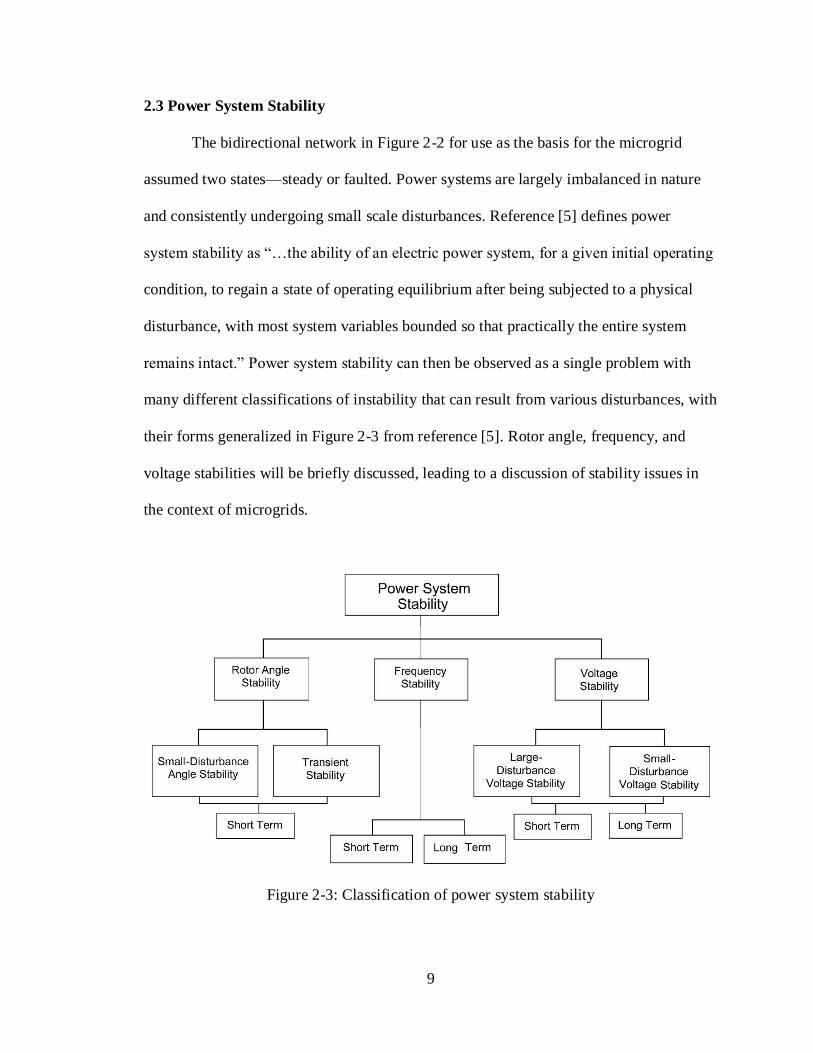
remains intact.” Power system stability can then be observed as a single problem with
many different classifications of instability that can result from various disturbances, with
their forms generalized in Figure 2-3 from reference [5]. Rotor angle, frequency, and
voltage stabilities will be briefly discussed, leading to a discussion of stability issues in
the context of microgrids.
Figure 2-3: Classification of power system stability

10
Rotor angle stability is concerned with synchronous machinery to retain
synchronism after perturbed by a disturbance. That is, stability in synchronous machinery
is largely concerned with a constant balancing of opposing electromagnetic and
mechanical forces. In steady-state conditions synchronous generators are assumed to be
operating at constant rotor angular speeds and electrical frequencies. However, the
equilibrium between input mechanical and output electromagnetic torques are
compromised as the generators experience a disturbance, with a deceleration or
acceleration of machines in response. For example, an electrical fault occurring near the
terminals of one generator can produce a large electromagnetic force, resulting in a
momentary imbalance with the mechanical torque of its rotor, moving the machine into a
transient state. As these machines begin to transfer power and attempt to reach a new
equilibrium point with a different rotor angular position with respect to another machine,
instability can result if synchronism cannot be achieved.
Voltage stability is largely concerned with variations in supply-load power
equilibrium in a system and maintaining stable bus voltages following a disturbance.
Reference [5] suggests “a major factor contributing to voltage instability is the voltage
drop that occurs when active and reactive power flow through inductive reactance of the
transmission network; this limits the capability of the transmission network for power
transfer and voltage support.” Following a disturbance, loads can drive the system into
instability by stressing power beyond equipment limitations and further varying bus
voltages until supply can no longer meet the electrical demands of the loads.
Frequency stability is concerned with maintaining a steady system frequency
following a disturbance in the system. Reference [5] claims “generally, frequency

11
stability problems are associated with inadequacies in equipment responses, poor
coordination of control and protection equipment, or insufficient generation reserve,”
with instability resulting in frequency swings leading to loss of loads or generating units.
Ultimately, there is crossover between various forms of instability that can arise in a
power system, with disturbances such as the clearing of a fault with a protective relay
transitioning a power system into a transient state with varying system parameters. That
is, power flow, bus voltages, and machine rotor speeds can all vary following the
disturbance, with voltage and frequency variations as a result as system stability is
compromised.
2.4 Microgrid Transient Stability Analysis
Stability in a microgrid shares similarities with classical power system stability
classifications shown in Figure 2-3, with additional issues such as disturbances resulting
from islanding. Reference [6] suggests “with micro sources with current limit, very little
spinning reserve and limited reactive support, it is essential to carry out detailed transient
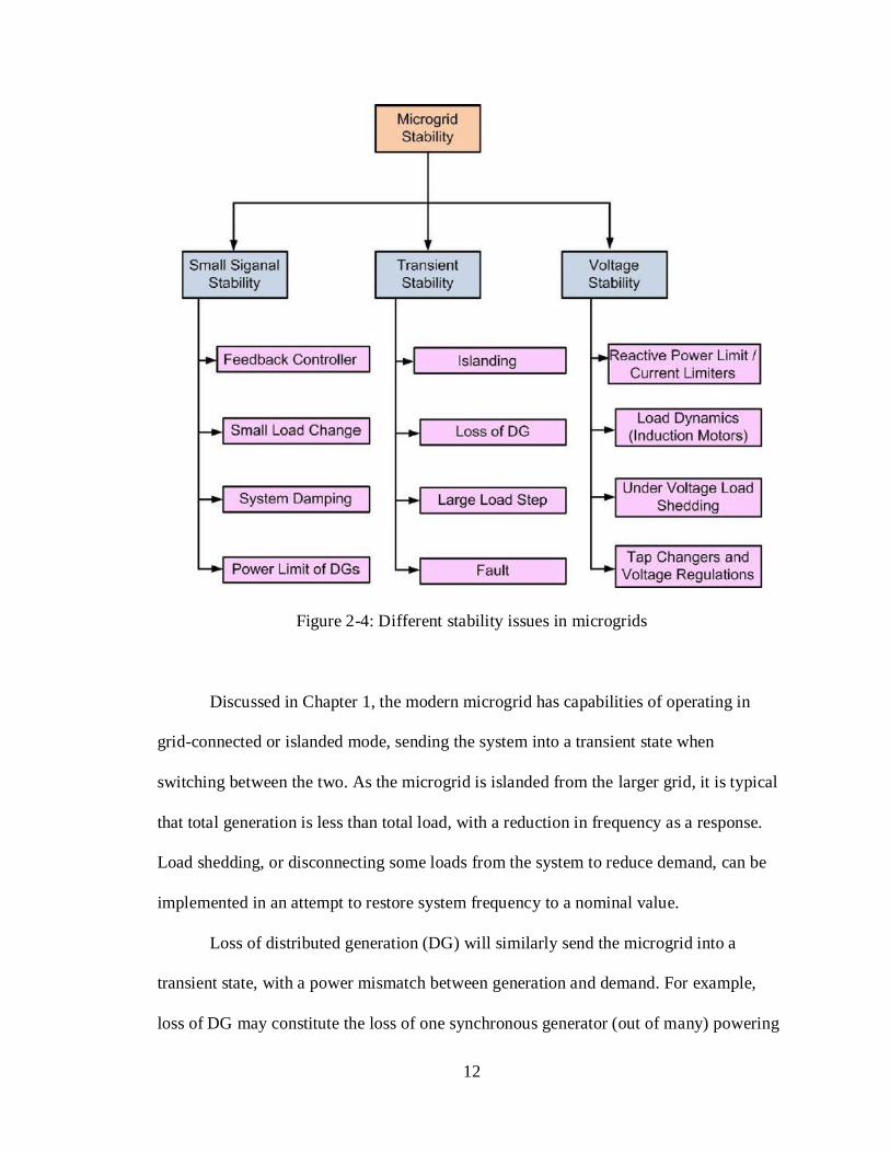
analysis with possible contingencies,” with Figure 2-4 showcasing microgrid stability
issues. Unlike microgrids with limited resources, the bulk power system typically has
excess generating capacity, or operating reserves, to meet real and reactive demands to
maintain stability.
12
Figure 2-4: Different stability issues in microgrids
Discussed in Chapter 1, the modern microgrid has capabilities of operating in
grid-connected or islanded mode, sending the system into a transient state when
switching between the two. As the microgrid is islanded from the larger grid, it is typical
that total generation is less than total load, with a reduction in frequency as a response.
Load shedding, or disconnecting some loads from the system to reduce demand, can be
implemented in an attempt to restore system frequency to a nominal value.
Loss of distributed generation (DG) will similarly send the microgrid into a
transient state, with a power mismatch between generation and demand. For example,
loss of DG may constitute the loss of one synchronous generator (out of many) powering

13
a microgrid, or the disconnection of a PV array as a generating unit. Load shedding will
again be required to maintain stability unless battery or storage devices are available to
supply the necessary power.
Lastly, electrical faults of all kinds will send the system into a transient state. An
ideal three-phase balanced power system will quickly transition into an unbalanced state
following a fault. For example, the opening of a line by a protective relay following a
fault will transition the system into a transient state with variations in load flow, bus
voltages, machine speeds, and frequency fluctuations. It is imperative to perform a
detailed system stability analysis to ultimately implement adequate islanding capabilities
for Cal Poly’s microgrid. As discussed in section 2.2, this thesis will first develop a
complete model of Cal Poly’s microgrid in ETAP with load flows, short circuits, and
protection coordination studies, eventually implementing and modeling future distributed
energy resources such as photovoltaics and battery storage systems. The latter portion of
this thesis will then use the model of Cal Poly’s microgrid in ETAP to ultimately perform
a system stability analysis, largely focused on microgrid transient stability issues
discussed and generalized in Figure 2-4.

14
Chapter 3: Design Requirements
3.1 System overview
This chapter proposes the framework in which the thesis objectives outlined in
Chapter 2 are to be achieved. The following decompositions characterizes the two main
thesis objectives—modeling the Cal Poly microgrid and performing a transient stability
analysis through ETAP software. Level zero decompositions establish the system-level
characteristics, followed by a summarization of parameters and specifications.
3.2 Functional Decomposition—ETAP Model
Figure 3-1 shows a level zero block diagram for the first phase of this thesis,
developing the ETAP model of the Cal Poly microgrid.
ETAP
MODEL
Synchrounous Generator
Induction Motor
Static Load
Power Transformer
Utility Grid
Protective Elements
Busbars
Cables
Solar Photovoltaic
Battery Storage
Load Flow
Short Circuit Analysis
Protection Coordination
Figure 3-1: ETAP Model Block Diagram, Level 0

15
Inputs to the ETAP model block diagram include the entirety of the existing Cal
Poly microgrid including the synchronous generators, induction motor, static loads,
power transformers, utility grid, protective elements (e.g. circuit breakers, relays),
busbars, and cables. Input devices that are currently not implemented in the existing
microgrid include solar photovoltaics and battery storage systems. However, these
modules will ultimately be modeled in ETAP to explore and analyze the functionality of
the microgrid as the project develops.
Outputs to the ETAP model block diagram in Figure 3-1 include load flow, short
circuit analysis, and protection coordination. ETAP Load Flow Analysis module will be
utilized to determine bus voltages, power factors, currents, and power flows throughout
the Cal Poly microgrid system. Capable of integrating and modeling swing, voltage
regulated, and voltage unregulated power supplies with several power grids and generator
connections, load flow studies of the microgrid can be sufficiently conducted through
ETAP software. To determine bus voltages, angles, and power flows, ETAP Load Flow
allows several different load flow calculation methods including Newton-Raphson, Fast-
Decoupled, and Gauss-Siedel. To perform the load flow study, each method contains
different load flow converging characteristics, allowing flexibility to meet the microgrid
system parameters including generation, loading conditions, and initial bus voltages. A
complete analysis of load flow methods and simulations for the microgrid will be
described and analyzed in future chapters of this thesis.
The ETAP Short Circuit analysis program will be utilized to analyze the fault
currents for three-phase, line-to-ground, line-to-line, and line-to-line-ground faults in the
microgrid. ETAP is able to calculate the total short circuit current contribution from
16
microgrid elements including the synchronous generators, induction motor, and utility
connections. ETAP includes both American National Standards Institute/Institute of
Electrical and Electronics Engineers (ANSI/IEEE) and International Electrotechnical
Commission (IEC) standards to perform its short circuit calculation methods. A complete
analysis of short circuit methods and its simulations for the microgrid will be described
and analyzed in future chapters.
The microgrid will utilize ETAP Star, the protection and coordination (selectivity)
module within ETAP. ETAP Star is equipped with a comprehensive protective device
library, able to accurately model protective elements (e.g. SEL relays) to perform
equipment protection and device coordination studies. ETAP Star Time Current
Characteristic (TCC) views will be generated to display device characteristic curves.
ETAP Star is also capable of determining operating times of protective devices by
simulating faults on the one-line diagram. A complete analysis of protection and device
coordination methods and its simulations for the microgrid will be described and
analyzed in future chapters.
3.3 Functional Decomposition—Transient Analysis
Figure 3-2 shows a level zero block diagram for the second phase of this thesis,
performing a transient stability analysis of the Cal Poly microgrid through ETAP
software.

17
Transient
Stability
Faults
Loss of DG
Large Load Step
Islanding
Power Flow variation
Stability improvement
Frequency variation
Machine dynamics
Voltage variation
Figure 3-2: Transient Stability Block Diagram, Level 0
The ETAP Transient Stability module will be utilized to investigate the microgrid
system dynamic responses and stability limits of the power system before, during, and
after system disturbances, characterized as the inputs in Figure 3-2. ETAP Transient
Stability will be utilized to investigate system responses including determining machine
power angles and speed variations, system electrical frequencies and voltages, real and
reactive power flows, determining critical fault clearing times, and testing relay settings.
Synchronous machinery will play a crucial role in power system stability as their power
(rotor) angles will oscillate and result in power flow oscillations in the microgrid
following a disturbance. In order to retain system stability, methods of improving
microgrid transient stability will be investigated, generalized from reference [6] in Figure
3-3. Control of battery storage, load shedding methods, protective device settings, and
control of power electronics can all be simulated within ETAP software. It is the goal of

18
the second phase of this thesis to analyze stability issues within the Cal Poly microgrid
and investigate methods of improving transient stability.
Figure 3-3: Microgrid Stability Improvement

19
Chapter 4: Design
4.1 Chapter overview
This chapter develops the framework for the ETAP model of the Cal Poly
microgrid accomplishing the goals set out and decomposed in Chapter 3. We begin with
the development of the ETAP model with justifications and assumptions needed for
system components and their parameters. An overview with examples and modeling of
load flow, short circuit, protective device coordination, and transient stability studies in
ETAP is developed and outlined in this chapter. The ETAP examples conducted
throughout this chapter are not of the Cal Poly microgrid, and instead are performed to
provide the reader a background to introductory case studies for power system studies
(e.g. protection coordination, transient stability). Simulations, results, and analyses for
case studies specific to the Cal Poly microgrid will be presented in Chapter 5.
4.2 ETAP Model
This section serves to provide preliminary information for all the system
components used in the ETAP model, and the parameters that are relevant in the scope of
this thesis (e.g. performing load flow, transient stability studies). Device parameters that
must be modified for certain case studies will be noted throughout simulations in Chapter
5. Figure 4-1 showcases the one-line diagram created in ETAP modeling the current
iteration of the Cal Poly microgrid as of winter quarter of 2018.
20
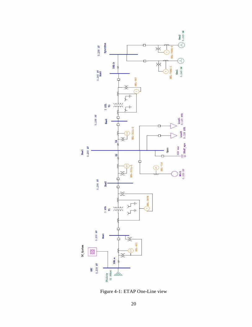
Figure 4-1: ETAP One-Line view
21
The ETAP Cal Poly microgrid elements in Figure 4-1 include the power grid,
impedances, circuit breakers, power transformers, three-phase induction motor, static
loads, circuit breakers, current transformers (CTs), potential transformers (PTs/VTs), and
protective relays. Power system elements not shown in Figure 4-1 include future
additions such as solar photovoltaics, inverters, and energy storage modules. Generating
units are shown in green, electrical loads in purple, and protective relays in orange.
The Power Grid element in ETAP models the utility interconnection with the
microgrid. The Cal Poly microgrid utilizes 208V and 240V three-phase AC voltages,
modeled as the utility supply voltage throughout this thesis. As such, the Power Grid is
rated for 208V operating in swing mode. In ETAP load flow studies, an element in swing
(slack) mode operation is used to balance power flow (active and reactive), with a voltage
magnitude and angle at the terminals remaining at set operating values. The Power Grid
in ETAP is modeled with its Thevenin’s equivalent, a constant voltage source behind a
short-circuit impedance. The Short Circuit page in the Power Grid editor provides
information necessary to model the utility grid as a source for studies including Short
Circuit and Transient Stability, to be discussed in latter portions of this chapter. Relevant
data include line voltage, short-circuit MVA, three phase fault currents, and X/R ratios.
The Impedance elements in ETAP are utilized to model 10Ω resistors and 45mH
inductors existing in the Cal Poly microgrid. The resistors in the microgrid are utilized
for current-limiting purposes for safely testing power system faults. The inductors are
utilized to model transmission lines of a power system. Although there exists a detailed
Transmission Line and Reactor elements in ETAP, it is unnecessary in the modeling of
inductors utilized in the microgrid.

22
The Power Transformer element in ETAP models two-winding three single-phase
transformers in the Cal Poly microgrid with a 1:1 turns ratio rated at 3KVA, 240V, and z
= 2.5%. The transformers were included to more accurately model a complete power
system and utilized for protective relaying experimentation by prior Cal Poly students.
Two power transformers are modeled connected in wye-wye configurations.
The Induction Machine element in ETAP models the three-phase induction motor.
The ETAP element models the Hampden IM-100, a one-third horsepower three-phase,
four pole, and squirrel cage motor with a wound stator and a squirrel cage rotor, utilized
for loading purposes. Induction motor power and impedance parameters will play a role
into short circuit and stability simulations, to be discussed in latter portions of this
chapter. Due to resistive losses in the system, voltages applied at the terminals of the
induction motor will be less than 208Vac in a laboratory setting. Induction motor
parameters will be largely based on laboratory tested ratings rather than nameplate
ratings.
The Static Load element in ETAP models two Hampden RLC-100
resistive/reactance loads utilized in the microgrid. The loads are connected in parallel,
providing resistive loading controlled by 6 toggle switches (12 total), each one inserting a
2000Ω resistor in parallel in each leg simultaneously (to a minimum of 167Ω). That is, at
maximum loading the two three-phase static loads consume a total of 2∗3∗(120𝑉𝐿𝑁 )2
333𝛺 =
259W at a nominal 208Vac line-to-line. Due to resistive losses in the system, voltages
applied to the static loads will be less than 208Vac in a laboratory setting. Static load
parameters will be largely based on laboratory tested ratings rather than nominal values.

23
The Synchronous Generator element in ETAP models two Hampden SM-100-3,
three-phase, four pole machines consisting of a wye/delta stator and quadrature rotor
having a DC field winding and a damper winding. DC field excitation is controlled by an
external variable resistor (rheostat) supplied by 125V DC. The rotor of the synchronous
generator is driven by a DC machine, Hampden DM-100 providing one-third horsepower
at 1800 rpm. Synchronous generator modeling is crucial in short circuit and stability
studies, and justifications will be provided in the following sections for modeling
machine impedances. SEL microprocessor based relays will be utilized to obtain
oscillograms of the generator current and voltage characteristics, in which short circuit
characteristics can be extracted.
The Relay elements in ETAP models Schweitzer Engineering Laboratory (SEL)
microprocessor based protective relays, heavily based on previous work per reference [4].
Models include SEL-387E, SEL-311L, SEL-710, SEL-587, SEL-700G, and SEL-421. A
complete analysis of protective device coordination will be conducted in later sections
and chapters, detailing zones of protection (e.g. transformer, induction motor), protection
schemes utilized (e.g. differential, directional, time-delay overcurrent), and protection
device settings. Current transformers (CTs) and potential transformers (VTs/PTs) shown
in the ETAP model are utilized to feed SEL relays electrical quantities to determine the
status of the microgrid. Due to low nominal and fault currents, the CTs and PTs are
included in the one-line diagram to adhere with ETAP modeling standards, and do not
exist in the hardware implementation. Therefore, the CTs and PTs throughout the ETAP
model have a 1:1 turns ratio. More information can be found in Protection Device
Coordination section in 4.5 for a background on protection fundamentals.

24
Figure 4-2 showcases a subsystem of the ETAP model of what the future Cal Poly
microgrid may consist of. There are currently no renewable energy resources or energy
storage systems utilized in the microgrid. Small scale solar photovoltaic generation
complete with an inverter to interconnect with the microgrid is a logical addition to the
system. ETAP consists of in depth solar photovoltaic and inverter modeling tools to
accurately represent Cal Poly’s renewable integration with the microgrid. ETAP is also
equipped with maximum power point (MPP) tracking control capabilities with its solar
inverters to adjust operating points for solar panels to extract maximum power. The SEL-
751 in Figure 4-2 can provide additional protective capabilities to the system.
Figure 4-2: ETAP Microgrid PV Subsystem

25
As an example, a PV module tentatively chosen for the Cal Poly microgrid
modeling purposes is the SUNTECH STP210. Figure 4-3 displays the PV Array editor
when double left clicking the PVA1 module in Figure 4-3. Under the PV Panel page, the
P-V curves display the power-voltage characteristics of a solar module for various levels
of solar irradiance, a measure of energy in the form of sunlight. Similarly, the nonlinear I-
V curves describe the current-voltage characteristics of the solar cells for various levels
of irradiance. ETAP has extensive libraries for various power system components, and
the curves and parameters shown in Figure 4-3 are populated when selecting the STP210
module from the library. Alternatively, a user can generate these curves individually by
creating an ETAP PV Array library file given known equivalent circuit parameters of a
solar cell, providing users with tools to accurately model a PV system.
26
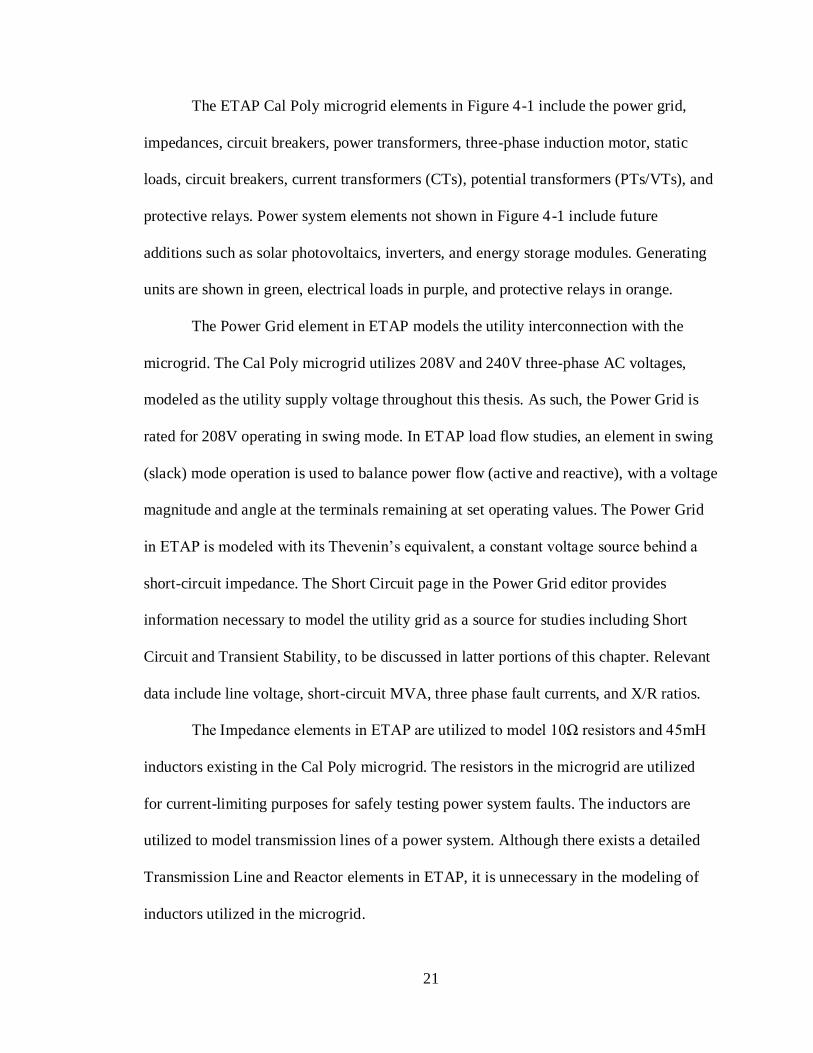
Figure 4-3: PV Array Editor
The ETAP Inverter will be utilized to convert the DC characteristics from the PV
array into the three-phase AC system, modeling the grid-tie inverter. The Inverter Editor
is a powerful tool that can control and modify several parameters including converter’s
efficiency, generation for AC Load Flow calculations, and harmonics of the device.
Power quality considerations can be analyzed by harmonics analysis tools in ETAP, and
Figure 4-4 displays the Harmonic tab of the grid-tied inverter. Similar to the PV Array
Editor in Figure 4-4, the harmonics of a specific device can be chosen from a list of
libraries in ETAP or entered given device characteristics. It is the objective that these
tools will be useful for the future Cal Poly microgrid students for the investigation of
power quality considerations in the system, and the utilization of SEL relays in
conjunction with performing proper courses of action.

27
Figure 4-4: Inverter Editor
Additionally, energy storage systems can be appended as additional generation
and loading systems. Additional SEL relays can be utilized with solar integration to
provide a more dynamic element to the system. That is, SEL relays can continually sense
electrical quantities including voltages, currents, and frequencies from a PV subsystem to
determine if curtailment or generation of renewable energy is necessary. This can further
lead to stability improvement methods, with control of power electronics providing many
advantages to the microgrid. Latter chapter will discuss the feasibility and simulations of

28
power electronics improvement of microgrid transient stability. Possible load flows, short
circuit, and transient stability studies of future microgrids will be conducted following the
analysis of the current iteration of the microgrid.
4.3 Load Flow Modeling
The main purpose of a load flow is to determine the balanced three-phase steady
state operation of the Cal Poly microgrid. Specifically, the solution to the load flow
problem will provide us with bus voltages and angles, as well as real and reactive power
flow. The load flow study will be performed in ETAP to meet the microgrid requirements
of generation adequately supplying the demand (load) and losses, bus voltages close to
nominal values, generation operating within active and reactive power limits, and
transmission line (inductor) and transformers not overloaded [11]. Equipment operating
values against manufacturer’s specified maximum capability ratings will be compared
when available.
The load flow study will consider several different operation scenarios such as
maximum loading, minimum loading, normal loading, grid-connected, and islanded
conditions. As an example, consider Figure 4-5 which displays the ETAP Study Case
editor for Load Flow Analysis Mode which will be heavily utilized for other modeling
simulations as well (short-circuit, transient, protection coordination).

29
Figure 4-5: Load Flow Study Case Editor
The Loading tab of the Load Flow Study Case editor shows Generation Category
operating under Design. This forces the Load Flow study to consider all generating units
in ETAP to operate under their Design operating conditions. For example, if we double
left click a synchronous generator in the ETAP one-line, we open the Synchronous
Generator Editor whose Design category is set to operate at 0.2 kW and 0.05 kvar,
illustrated in Figure 4-6. The Synchronous Generator is set to operate under Mvar Control
instead of Swing Control in the Info page (not shown), to set fixed active and reactive

30
power output of the machines. This will be useful as we can perform accurate case
studies for generators outputting specific active and reactive power. Additionally, this is
also due to the inherent limitations of the microgrid in which we do not implement
generator exciter and governor control, to be further explained in the Transient Stability
section. The interested reader can refer to section 4.5.2 for an ETAP example of a load
flow leading to protective device coordination.
Figure 4-6: Synchronous Generator Editor

31
The above procedure will be detailed in depth throughout various Load Flow case
studies in Chapter 5, with different loading and generating conditions. Additional load
flows will be also conducted on the consideration of future iterations of the microgrid lab
including devices such as photovoltaics, inverters, and battery storage. Finally, computer
generated analysis reports will be provided to summarize a comparison of power flow
results from different operating considerations.
4.4 Short Circuit Analysis Modeling
The main purpose of a short circuit study in the context of the Cal Poly microgrid
lab is to ultimately determine appropriate ratings and settings for protective relay
coordination by analyzing the effect of different faults injected in the system. Short
circuit studies enable verification of protective device interrupting capabilities (e.g.
circuit breakers), as well as protect equipment from large electromagnetic and mechanical
forces due to high fault currents. However, fault currents in the Cal Poly microgrid are
deliberately minimized due to safety considerations, and as a result of utilizing smaller
rated equipment (e.g. 1/3rd horsepower motors and generators). ETAP elements that
contribute to a short-circuit fault current include synchronous machines, induction
machines, and the power (utility) grid. Additional modifications to the microgrid
including inverters and batteries will also contribute to short-circuit currents.

32
4.4.1 Short Circuit Analysis Overview
Section 4.4.1 serves to provide preliminary information on the fundamentals of
short circuit analysis for the interested reader. Additionally, section 4.4.1 can be used as a
reference for ETAP simulations in Chapter 5. We begin the overview of short-circuit
analysis with an overview of symmetrical components. The method of symmetrical
components is of fundamental importance to analyze and simplify an unbalanced power
system during the event of a fault (short-circuit) or disturbance, allowing us to convert a
three-phase unbalanced system into a set of balanced phasors that we term symmetrical
or sequence components. Consider Figure 4-7 which summarizes the resolving of
unbalanced voltage phasors into a set of balanced sequence components [8]. The α
operator is a complex number whose magnitude is 1 with a phase angle of 120°, and α2
has magnitude 1 with phase angle of 240°. V0, V1, V2 are the zero, positive, and negative
sequence components respectively, which can be further decomposed to individual
balanced sequence components (e.g. V2 negative sequence phasor can be decomposed to
Va2, Vb2, Vc2).

33
Figure 4-7: Symmetrical Components of three balanced phasors [8]
Notice that if we definite matrix operator A and its inverse A as
𝑨 = [1 1 11 α2 α1 α α2
], 𝑨−𝟏 =1
3[1 1 11 α α2
1 α2 α
] (4-1)
then one can transform phase values into sequence components and vice versa as shown
in equation 4-2.
[𝑉𝑎
𝑉𝑏
𝑉𝑐
] = 𝑨 ∙ [𝑉𝑎0𝑉𝑎1𝑉𝑎2
], [𝑉𝑎0𝑉𝑎1𝑉𝑎2
] = 𝑨−𝟏 ∙ [𝑉𝑎
𝑉𝑏
𝑉𝑐
] (4-2)
Consider Figure 4-8 which illustrates the decomposition of an unbalanced system
with unbalanced voltage phasors as a summation of balanced sequence components [12].
That is, phasor voltage Va is the vector or phasor summation of symmetrical components
with positive-sequence phasor Va1, negative-sequence phasor Va2, and zero-sequence
phasor Va0. Notice that all positive, negative, and zero sequence components are
balanced, that is they are equal in magnitude indicated by the length of the vectors and

34
offset by 120° (e.g. positive-sequence components Va1, Vb1, Vc1). Zero sequence
components by definition have no offset.
Figure 4-8: Unbalanced voltage phasors, symmetrical components [12]
Several different faults exist in a power system, including line-to-ground, line-to-
line, line-to-line-to-ground, and three-phase faults. Depending on the type of fault that
has occurred, the power system can be decomposed into different sets of symmetrical
components and sequence networks for adequate fault analysis. Unbalanced current
phasors during the event of a short-circuit fault can also be decomposed into a set of
balanced positive, negative, and zero sequence components similar to that of voltage
phasors, which is instrumental in the analysis of fault currents. Symmetrical components
are fundamental to understand an adequate protection as the protective relays utilized in
the Cal Poly microgrid (SEL relays) perform the decomposition shown in Figure 4-8.

35
For example, the SEL relays are continually sensing voltage and current phasors,
decomposing unbalanced quantities into a set of balanced symmetrical components, and
asserting relay trip commands to circuit breakers in the event of a fault. Coordination will
be analyzed in detail in further sections—however, ETAP Short-Circuit analysis module
will be heavily utilized in conjunction with ETAP Star (protection) module to analyze
fault currents, their decompositions into symmetrical components, and adequately
implementing protection that accurately models the hardware implementation for SEL
relays. It will be imperative for the future Cal Poly microgrid team to understand the
method of symmetrical components to adequately implement relay settings, and it is the
objective that ETAP Short-Circuit module will help them accomplish this task as the
microgrid increases with complexity with added fault contributions from distributed
resources (e.g. solar panels, battery storage).
Let us first consider the R-L circuit shown in Figure 4-9, in which the closing of
switch SW at time t = 0 represents a Thevenin equivalent of a three-phase short circuit at
the terminals of an unloaded synchronous machine.

36
Figure 4-9: R-L circuit short-circuit response [11]
Writing KVL for the circuit in Figure 4-9 results in
𝐿𝑑𝑖(𝑡)
𝑑𝑡+ 𝑅𝑖(𝑡) = √2𝑉𝑠𝑖𝑛(𝜔𝑡 + 𝛼) (4-3)
whose solution can be decomposed into a summation of currents iac and idc, summarized
in Table 4-1 where time constant T = L/R = 𝑋/(2𝜋𝑓𝑅) seconds, angle θ = tan-1(X/R)
degrees, Z = √𝑅2 + 𝑋2 Ω [11].

37
Table 4-1: Short-circuit current, series R-L circuit [11]
Of importance in equipment sizing and relay coordination is the worst case rms
asymmetrical fault current, which has a magnitude of √3Iac and decays to Iac as the dc
component of the fault current exponentially decays. It is important to note that this dc
offset current is dependent on the time in which the short circuit is initiated, and it is
incorrect to assume this dc offset current is a result of stored magnetic energy in inductor
L. Additionally, each phase of a three-phase synchronous machine would each have a
different dc offset, due to the varying magnitude of induced stator voltage at different
times during fault inception. In practical applications, protective devices such as circuit
breakers must be able to sustain this worst case scenario fault current without damage.
Let us now consider an oscillogram illustrating the response of one phase to a
three phase short circuit on the terminals of an unloaded synchronous generator shown in
Figure 4-10 [8].
38
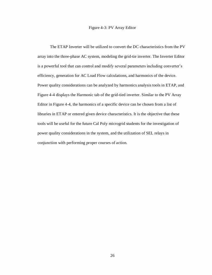
Figure 4-10: Armature short circuit current with dc offset removed
The instantaneous ac fault current can be written as [11]:
𝑖𝑎𝑐(𝑡) = √2𝐸𝑔 [(1
𝑋𝑑′′ −
1
𝑋𝑑′ ) 𝑒−𝑡/𝑇𝑑
′′
+ (1
𝑋𝑑′ −
1
𝑋𝑑) 𝑒−𝑡/𝑇𝑑
′+
1
𝑋𝑑] sin (𝜔𝑡 + 𝛼 −
𝜋
2) (4-4)
where 𝑋𝑑′′ is the direct axis subtransient reactance, 𝑋𝑑
′ is the direct axis transient
reactance, 𝑋𝑑 is the direct axis synchronous reactance, 𝑇𝑑′′ is the direct axis short-circuit
subtransient time constant, 𝑇𝑑′ is the direct axis short-circuit transient time constant [11].
As we can see from equation 4-4, the fault current on the terminals of a synchronous
machine can be modeled in three different stages, characterized by the specific reactance
and time since the fault has been initiated. For example, the highest peak fault current
exists at time t = 0 when equation 4-2 reduces to √2𝐸𝑔
𝑋𝑑′′ amps, where Eg is the assumed
constant pre-fault rms excitation voltage of the synchronous machine, also called the

39
voltage behind subtransient reactance. At t = ∞, equation 4-2 reduces to a steady state
fault current of peak magnitude √2𝐸𝑔
𝑋𝑑.
A summary of the instantaneous short-circuit fault current of 4-10 can be found in
Table 4-2 [11]. Parameters in Table 4-2 including machine reactances and time constants
can be found from analyzing an oscillogram similar to 4-10, or by obtaining them from
manufacturers. Therefore, the Hampden SM-100 3-phase synchronous machine will need
to be characterized and modeled with the parameters in Table 4-2 to obtain reliable
results in the analysis of short-circuit and transient stability studies. According to
Blackburn et al., “For system-protection fault studies, the almost universal practice is to
use the subtransient (𝑋𝑑′′) for the rotating machinery in the positive-sequence networks.
This provides a maximum value of fault current that is useful for high-speed relaying”
[12]. In this thesis oscillograms similar to that of Figure 4-10 will be extracted from SEL
events to characterize the parameters of a synchronous machine.
40
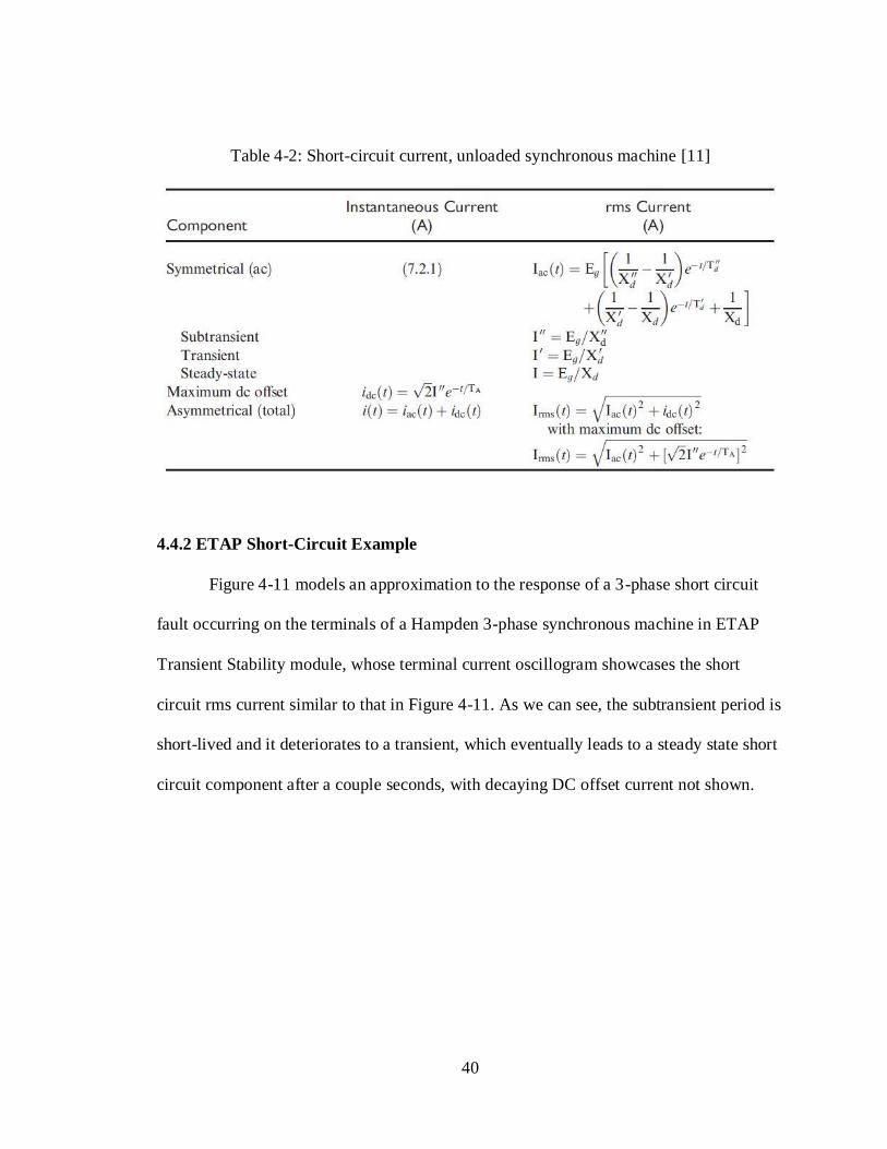
Table 4-2: Short-circuit current, unloaded synchronous machine [11]
4.4.2 ETAP Short-Circuit Example
Figure 4-11 models an approximation to the response of a 3-phase short circuit
fault occurring on the terminals of a Hampden 3-phase synchronous machine in ETAP
Transient Stability module, whose terminal current oscillogram showcases the short
circuit rms current similar to that in Figure 4-11. As we can see, the subtransient period is
short-lived and it deteriorates to a transient, which eventually leads to a steady state short
circuit component after a couple seconds, with decaying DC offset current not shown.

41
Figure 4-11: Extrapolation of asymmetrical AC fault current
In summary, ETAP Short-Circuit module will be utilized in the context of the Cal
Poly microgrid in two parts. First is to determine the symmetrical components associated
with different fault currents injected throughout the microgrid. A short circuit study is an
essential pre-requisite to adequately implement power system protection. Secondly,
short-circuit protection is also necessary to observe and extract the transient behavior of
rotating machinery following a fault. It is the objective of this thesis to match ETAP
generated oscillograms such as in Figure 4-11 with SEL relay event oscillograms to
ensure the accuracy of machine modeling. Once the transient parameters are discovered
and modeled accurately, we can begin to perform a transient stability study of the
microgrid.

42
4.5 Protective Device Coordination Modeling
This section on power system protection and device coordination will heavily
build upon the work of [4] which laid the framework of the Cal Poly microgrid protection
by prior students. As such, all protective relay elements utilized in ETAP will be models
of SEL relays implemented in the laboratory. One of the primary goals of this section is
not only to demonstrate protective relaying but also provide an intuitive and user-friendly
view of protective device coordination. This will be achieved by simulating the injection
of various faults throughout the microgrid system and observing the opening and closing
of protective devices such as circuit breakers in response. Although reference [4] laid
admirable groundwork in the development of the microgrid protection scheme, one area
missing from their documentation is an adequate background of symmetrical components
and their relation to fault currents. Additionally, the inclusion of Time-Current Curves
(TCC) will be useful for the future microgrid team to more easily implement protection
as the complexity of the system increases with added system components. It is the
objective of this thesis to bridge the gap between symmetrical components calculated in
ETAP to its hardware implementation with SEL relays in an intuitive and user-friendly
manner for the future Cal Poly microgrid team.
4.5.1 Protection and Coordination overview
Section 4.5.1 serves to provide preliminary information on the fundamentals of
power system protection and coordination for the interested reader. Additionally, section
4.5.1 can be used as a reference for ETAP simulations in Chapter 5. Power system

43
protection can be defined as the “science, skill, and art of applying and setting relays or
fuses, or both, to provide maximum sensitivity to faults and undesirable conditions, but to
avoid their operation under all permissible or tolerable conditions” [4]. That is, any
protection scheme implemented must be able to quickly detect faults or disturbances and
initiate appropriate control circuit action accordingly lest risk damaging equipment.
Additionally, it is imperative to properly coordinate equipment (e.g. protective relay
settings) for reasons including adequate backup protection.
System protection consists of three basic components, including instrument
transformers, protective relays, and circuit breakers. System-protection components need
to meet the following design criteria including reliability, selectivity, speed, economy,
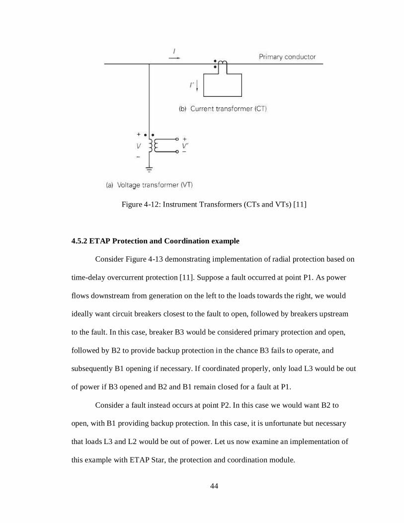
and simplicity, with varying degrees of criteria [11]. Consider instrument transformers
shown in Figure 4-12 showing voltage/potential transformers (VTs/PTs) and current
transformers (CTs). The purpose of these instrument transformers are to measure
electrical quantities and supply them as inputs to protective relays (not shown).
Secondary’s I’ and V’ are stepped down to nominal values such as 5 amps and 120Vac
line-to-neutral as dictated by the turns ratio of the instrument transformers. As mentioned
in section 4.2 the Cal Poly microgrid does not implement instrument transformers as
electrical quantities are at a minimum value, and primary currents/voltages are instead
directly fed to the SEL relays.
44
Figure 4-12: Instrument Transformers (CTs and VTs) [11]
4.5.2 ETAP Protection and Coordination example
Consider Figure 4-13 demonstrating implementation of radial protection based on
time-delay overcurrent protection [11]. Suppose a fault occurred at point P1. As power
flows downstream from generation on the left to the loads towards the right, we would
ideally want circuit breakers closest to the fault to open, followed by breakers upstream
to the fault. In this case, breaker B3 would be considered primary protection and open,
followed by B2 to provide backup protection in the chance B3 fails to operate, and
subsequently B1 opening if necessary. If coordinated properly, only load L3 would be out
of power if B3 opened and B2 and B1 remain closed for a fault at P1.
Consider a fault instead occurs at point P2. In this case we would want B2 to
open, with B1 providing backup protection. In this case, it is unfortunate but necessary
that loads L3 and L2 would be out of power. Let us now examine an implementation of
this example with ETAP Star, the protection and coordination module.

45
Figure 4-13: Single-line, Radial protection example [11]
Figure 4-14 demonstrates a load flow of the ETAP realization of the radial
protection example shown in Figure 4-13. For demonstration purposes, each relay utilizes
phase time-delay overcurrent protection (ANSI 51P) function from the SEL-311L
microprocessor based protective relays. The relays in this example are set with three
basic settings: pickup current or current tap setting, time-dial setting, and characteristics
curves. Pickup current is minimum current needed to initiate relay operation. For
example, the moment a fault current is transformed by the CT secondary and fed to the
relays, the relays determine whether this CT secondary exceeds the pickup current and
initiates relay operation. Time-dial settings are utilized to implement intentional time
delay prior to relay operation. Relay characteristic curves characterize the curvature of
the time curves and are a function of both time delay and pick up currents, defined by
equations. In our radial protection example we set our SEL relays with U2 inverse curves.
Time delays, pickup current, and curve types will be discussed further in the section from
an analysis of a Time-Current-Curve (TCC).
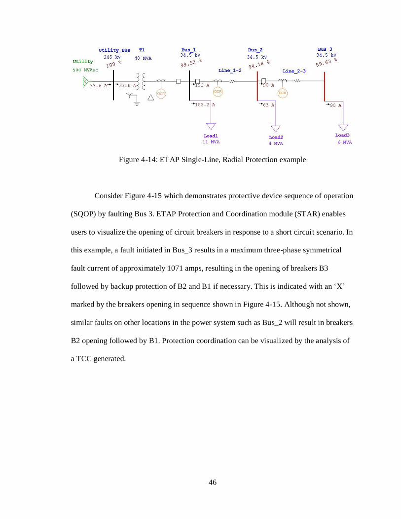
46
Figure 4-14: ETAP Single-Line, Radial Protection example
Consider Figure 4-15 which demonstrates protective device sequence of operation
(SQOP) by faulting Bus 3. ETAP Protection and Coordination module (STAR) enables
users to visualize the opening of circuit breakers in response to a short circuit scenario. In
this example, a fault initiated in Bus_3 results in a maximum three-phase symmetrical
fault current of approximately 1071 amps, resulting in the opening of breakers B3
followed by backup protection of B2 and B1 if necessary. This is indicated with an ‘X’
marked by the breakers opening in sequence shown in Figure 4-15. Although not shown,
similar faults on other locations in the power system such as Bus_2 will result in breakers
B2 opening followed by B1. Protection coordination can be visualized by the analysis of
a TCC generated.
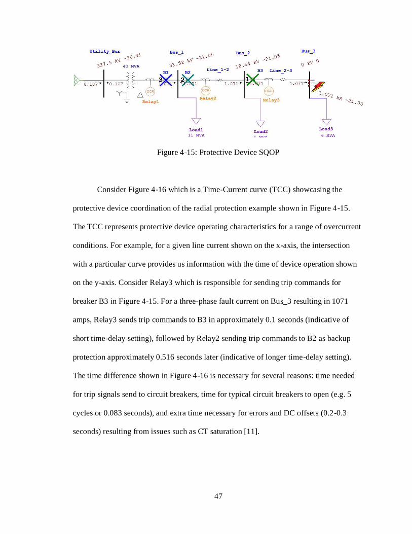
47
Figure 4-15: Protective Device SQOP
Consider Figure 4-16 which is a Time-Current curve (TCC) showcasing the
protective device coordination of the radial protection example shown in Figure 4-15.
The TCC represents protective device operating characteristics for a range of overcurrent
conditions. For example, for a given line current shown on the x-axis, the intersection
with a particular curve provides us information with the time of device operation shown
on the y-axis. Consider Relay3 which is responsible for sending trip commands for
breaker B3 in Figure 4-15. For a three-phase fault current on Bus_3 resulting in 1071
amps, Relay3 sends trip commands to B3 in approximately 0.1 seconds (indicative of
short time-delay setting), followed by Relay2 sending trip commands to B2 as backup
protection approximately 0.516 seconds later (indicative of longer time-delay setting).
The time difference shown in Figure 4-16 is necessary for several reasons: time needed
for trip signals send to circuit breakers, time for typical circuit breakers to open (e.g. 5
cycles or 0.083 seconds), and extra time necessary for errors and DC offsets (0.2-0.3
seconds) resulting from issues such as CT saturation [11].

48
Figure 4-16: TCC, Radial Protection example
Finally, let us modify the single-line diagram in Figure 4-15 to include a
secondary source of generation. Let us now observe the bidirectional system in Figure 4-
17 in which two sources of generation supply power to loads L1, L2, and L3 [11]. The

49
advantage in this configuration is that if properly coordinated, we are able to remove
faults occurring along the transmission lines at points P1 or P2 without the loss of any
load. For example, if a fault occurs on points P1, we can open breakers B23 and B32 and
power can still be fed from both sides to supply all the loads.
Figure 4-17: Bidirectional System with two sources [11]
However, the disadvantage of this bidirectional system is that we cannot
implement simple time-overcurrent protection to coordinate the opening of breakers
between relays. For example, time overcurrent is sufficient if we choose B21 as
secondary protection if B23 fails to open for a fault at P1. However, consider a fault on
point P2 with the same time overcurrent settings coordinated for a fault at P1. We would
want B12 and B21 to open and extinguish the fault at P2 and all loads are still fed power
from both sides. However, with the same time overcurrent settings for faults at P1, B23
would open quicker than B21, and we can no longer supply load L2 from generation on
the right.
In summary, the current iteration of the Cal Poly microgrid is very similar to that
of the bidirectional system is shown in Figure 4-17 in which time overcurrent protection
must be supplemented with other types of protection for proper coordination. It is

50
impossible for a bidirectional system to implement proper coordination with time
overcurrent alone, and thus we will utilize SEL relay capabilities to implement
coordination including distance and differential protections. Several case studies for
different faults initiated on the microgrid will be conducted, with sequence-of-operation
and time current curves illustrated throughout section 4.5.2 provided.
4.6 Transient Stability modeling
Load flow, short circuit analysis, and protective device coordination were
necessary studies leading up to the implementation of the second phase of this thesis:
transient stability analysis in microgrids. Discussed in Chapter 2, transient stability
involves the study of a power system and specifically synchronous machine rotor angle
response following a disturbance. We begin our study of transient stability with an
overview of the transient stability phenomena in classical power systems, implement a
transient stability example in ETAP, and justify any assumptions necessary in machine
modeling in the context of microgrid transient stability.
4.6.1 Transient Stability overview
This section serves to provide preliminary information on the fundamentals of
power system transient stability for the interested reader. Additionally, this section can be
used as a reference for ETAP simulations in Chapter 5. Consider Figure 4-18 which
showcases a mechanical analogy of the transient stability phenomenon in bulk power
systems [11]. Each suspending mass can represent a large synchronous machine drawing
or providing electric power, with the strings representing transmission lines holding the
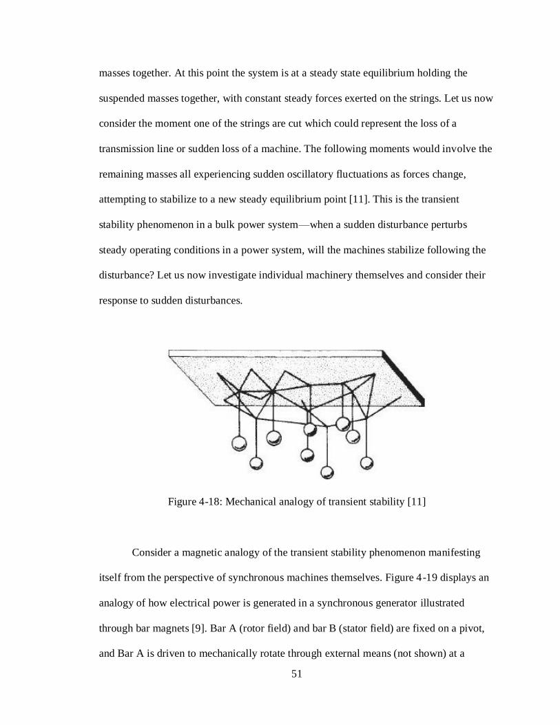
51
masses together. At this point the system is at a steady state equilibrium holding the
suspended masses together, with constant steady forces exerted on the strings. Let us now
consider the moment one of the strings are cut which could represent the loss of a
transmission line or sudden loss of a machine. The following moments would involve the
remaining masses all experiencing sudden oscillatory fluctuations as forces change,
attempting to stabilize to a new steady equilibrium point [11]. This is the transient
stability phenomenon in a bulk power system—when a sudden disturbance perturbs
steady operating conditions in a power system, will the machines stabilize following the
disturbance? Let us now investigate individual machinery themselves and consider their
response to sudden disturbances.
Figure 4-18: Mechanical analogy of transient stability [11]
Consider a magnetic analogy of the transient stability phenomenon manifesting
itself from the perspective of synchronous machines themselves. Figure 4-19 displays an
analogy of how electrical power is generated in a synchronous generator illustrated
through bar magnets [9]. Bar A (rotor field) and bar B (stator field) are fixed on a pivot,
and Bar A is driven to mechanically rotate through external means (not shown) at a
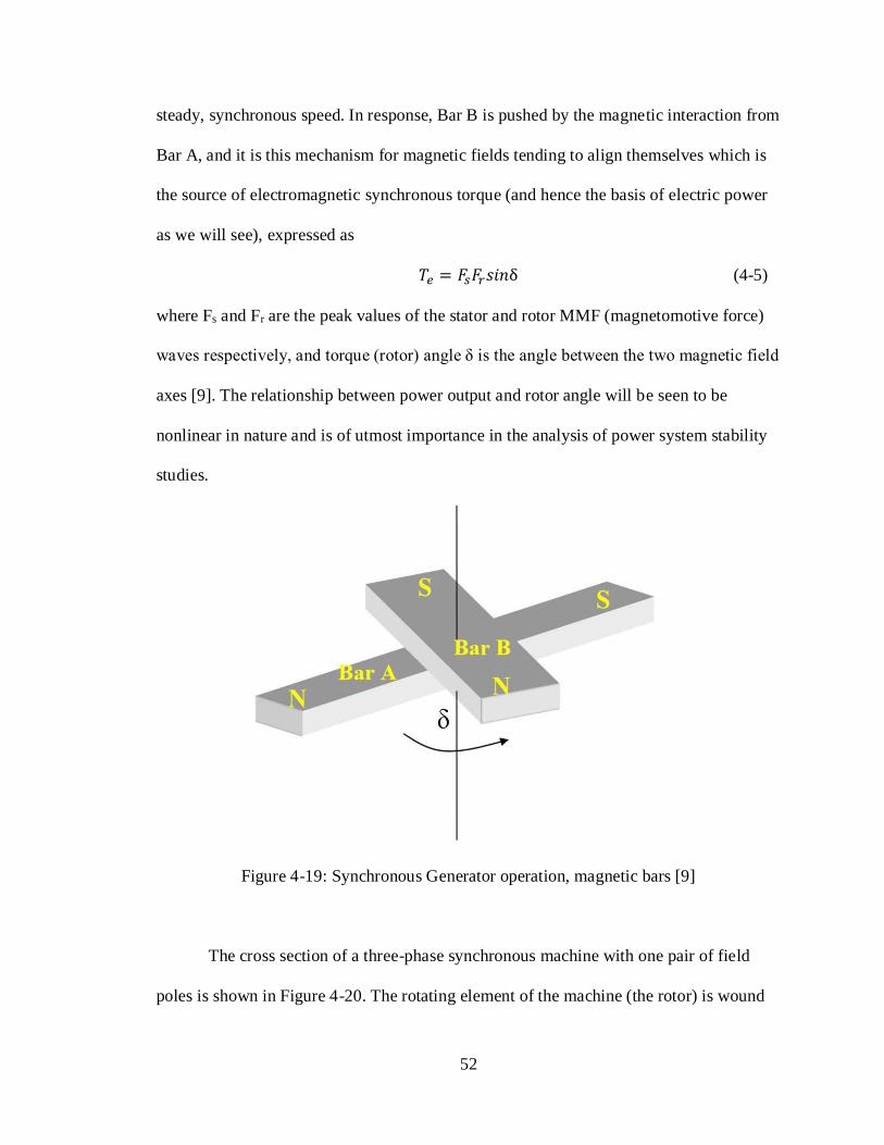
52
steady, synchronous speed. In response, Bar B is pushed by the magnetic interaction from
Bar A, and it is this mechanism for magnetic fields tending to align themselves which is
the source of electromagnetic synchronous torque (and hence the basis of electric power
as we will see), expressed as
𝑇𝑒 = 𝐹𝑠𝐹𝑟𝑠𝑖𝑛δ (4-5)
where Fs and Fr are the peak values of the stator and rotor MMF (magnetomotive force)
waves respectively, and torque (rotor) angle δ is the angle between the two magnetic field
axes [9]. The relationship between power output and rotor angle will be seen to be
nonlinear in nature and is of utmost importance in the analysis of power system stability
studies.
Figure 4-19: Synchronous Generator operation, magnetic bars [9]
The cross section of a three-phase synchronous machine with one pair of field
poles is shown in Figure 4-20. The rotating element of the machine (the rotor) is wound
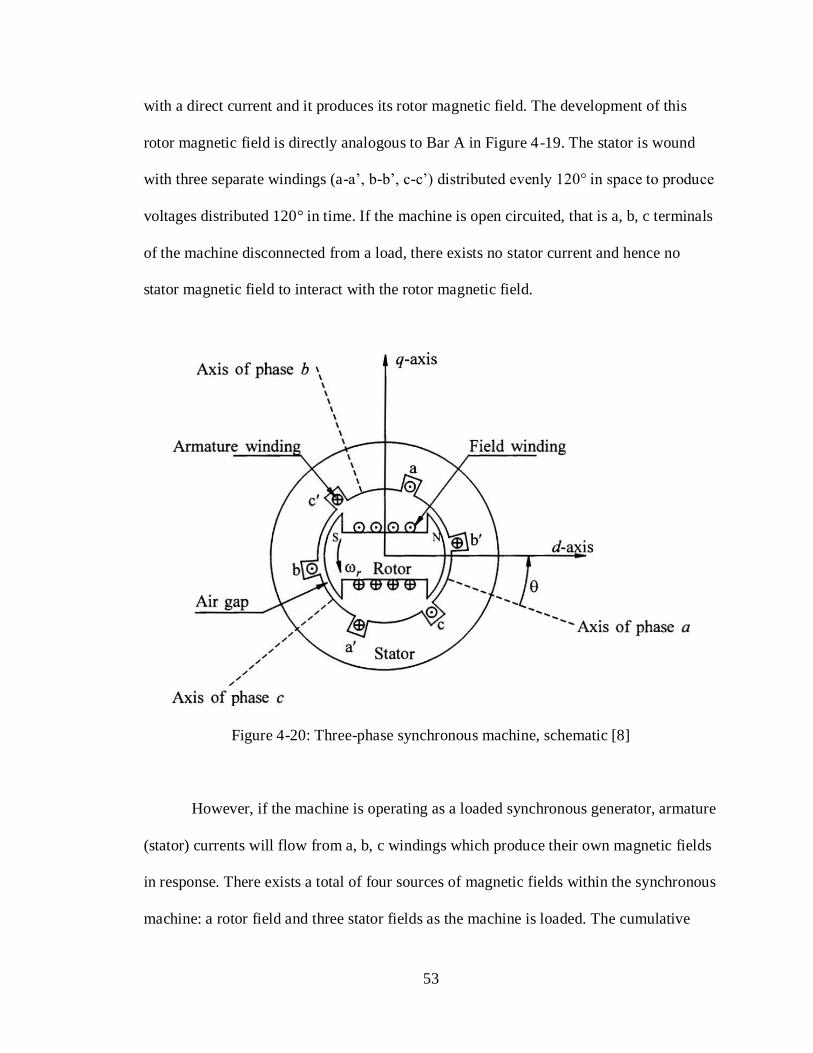
53
with a direct current and it produces its rotor magnetic field. The development of this
rotor magnetic field is directly analogous to Bar A in Figure 4-19. The stator is wound
with three separate windings (a-a’, b-b’, c-c’) distributed evenly 120° in space to produce
voltages distributed 120° in time. If the machine is open circuited, that is a, b, c terminals
of the machine disconnected from a load, there exists no stator current and hence no
stator magnetic field to interact with the rotor magnetic field.
Figure 4-20: Three-phase synchronous machine, schematic [8]
However, if the machine is operating as a loaded synchronous generator, armature
(stator) currents will flow from a, b, c windings which produce their own magnetic fields
in response. There exists a total of four sources of magnetic fields within the synchronous
machine: a rotor field and three stator fields as the machine is loaded. The cumulative

54
effects of stator magnetic fields are directly analogous to Bar B in Figure 4-19. That is,
balanced three-phase currents in the armature windings result in a single rotating stator
magnetic field from the perspective of the rotor in the air-gap rotating at synchronous
speed. Therefore, a production of steady electric torque is developed if the stator and
rotor fields rotate at the same speed, conceptualized as Bar A and Bar B rotating
synchronously. When there is variation of these magnetic fields, whether by speed or
magnitude (e.g. fault on generator terminals, increase in loading conditions), the resultant
variations in flux linkages throughout the machine will invariable affect rotor angle δ,
which is the essence of the transient stability phenomena.
4.6.2 ETAP Transient Stability Example
Let us now investigate an elementary example of transient stability in ETAP,
which will serve as an introduction to stability simulations for the Cal Poly microgrid in
Chapter 5. Figure 4-21 represents a system in which a generator is supplying power to an
infinite bus represented as the power grid through two transmission lines [8]. Bus HT is
suddenly disturbed with a three-phase bolted fault following a steady state scenario.

55
Figure 4-21: ETAP implementation of faulted bus
Figure 4-22 displays a plot of the rotor angle response of the generator with
respect to time following the faulted scenario. In this ETAP example the power grid
represents an infinite bus and is modeled as the swing bus with a reference angle of 0°.
We assume the input mechanical power driving the generator is constant throughout this
study. Prior to time t = 1 seconds, the system is assumed to be at a pre-fault steady state
with the generator supplying power to the infinite bus. At time t=1 second the three-phase
fault is applied on bus HT, and in response the generator experiences a variation from its
initial internal rotor angle δ of about 92°. Due to inertial effects, the rotor angle cannot
change instantaneously, but increases from its initial value as mechanical power is greater
than electrical power supplied. At time t = 1.05 seconds, the fault is cleared, but the rotor
angle does not settle to a steady state value immediately. The oscillatory nature of the
rotor angle response is due to a constant acceleration and deceleration of the rotor as it
stores and releases kinetic energy, attempting to reach a steady state operating point at a

56
new fixed rotor angle in which mechanical power input is matched with electrical power
output.
Figure 4-22: Rotor angle response, fault cleared in 0.05 seconds
Consider Figure 4-23 which represents the variation in generator electrical power
with respect to time during the disturbance. As the generator is initially delivering power
prior to time t=1 second at the steady state operating condition, its electrical power drops
nearly to 0 as the fault is initiated. The non-zero electrical power demonstrates resistive
losses in the system, and in a purely reactive system there would be no power delivered
to the infinite bus during this scenario for a fault at HT. As the fault is cleared at t=0.05
seconds, electrical power delivered still manifests itself in an oscillatory manner as the
rotor angle varies.
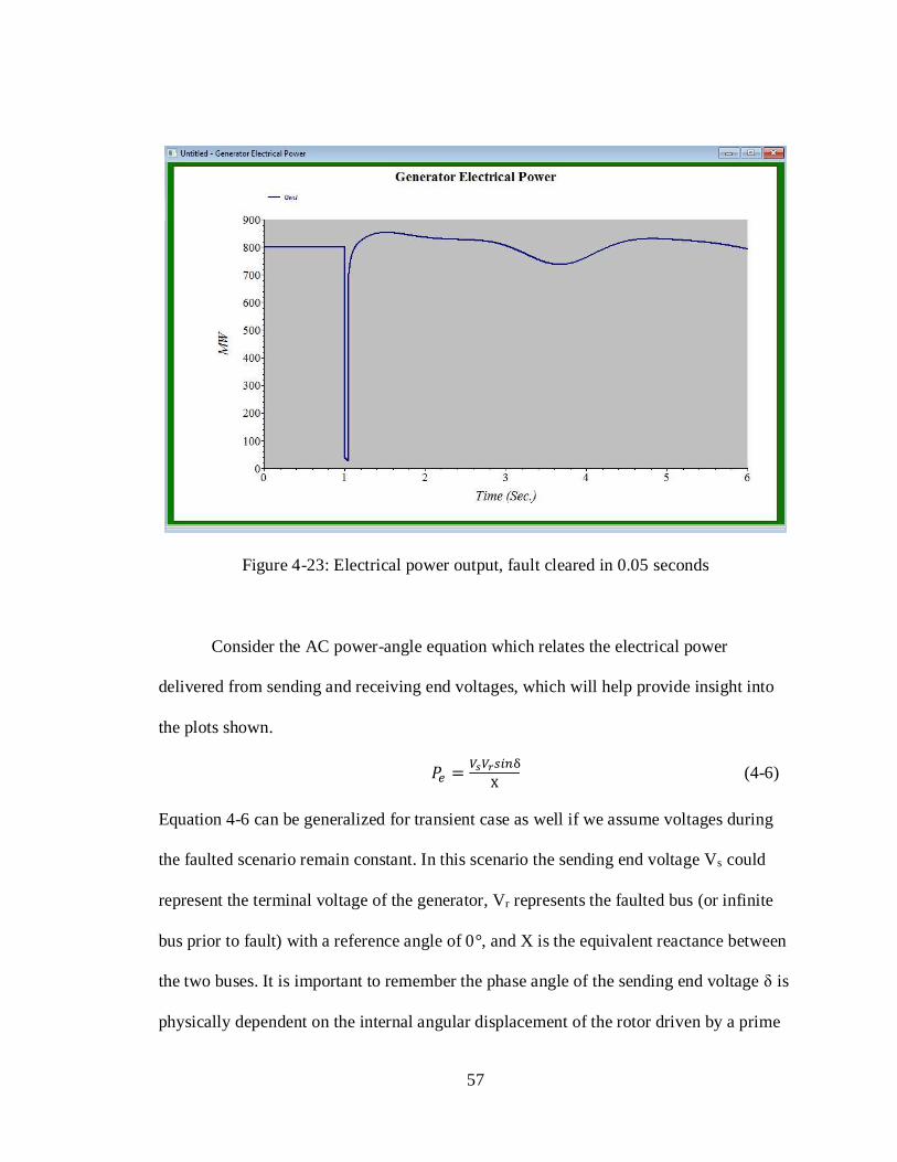
57
Figure 4-23: Electrical power output, fault cleared in 0.05 seconds
Consider the AC power-angle equation which relates the electrical power
delivered from sending and receiving end voltages, which will help provide insight into
the plots shown.
𝑃𝑒 =𝑉𝑠𝑉𝑟𝑠𝑖𝑛δ
X (4-6)
Equation 4-6 can be generalized for transient case as well if we assume voltages during
the faulted scenario remain constant. In this scenario the sending end voltage Vs could
represent the terminal voltage of the generator, Vr represents the faulted bus (or infinite
bus prior to fault) with a reference angle of 0°, and X is the equivalent reactance between
the two buses. It is important to remember the phase angle of the sending end voltage δ is
physically dependent on the internal angular displacement of the rotor driven by a prime
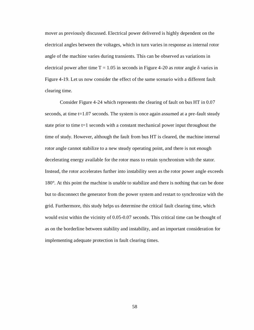
58
mover as previously discussed. Electrical power delivered is highly dependent on the
electrical angles between the voltages, which in turn varies in response as internal rotor
angle of the machine varies during transients. This can be observed as variations in
electrical power after time T = 1.05 in seconds in Figure 4-20 as rotor angle δ varies in
Figure 4-19. Let us now consider the effect of the same scenario with a different fault
clearing time.
Consider Figure 4-24 which represents the clearing of fault on bus HT in 0.07
seconds, at time t=1.07 seconds. The system is once again assumed at a pre-fault steady
state prior to time t=1 seconds with a constant mechanical power input throughout the
time of study. However, although the fault from bus HT is cleared, the machine internal
rotor angle cannot stabilize to a new steady operating point, and there is not enough
decelerating energy available for the rotor mass to retain synchronism with the stator.
Instead, the rotor accelerates further into instability seen as the rotor power angle exceeds
180°. At this point the machine is unable to stabilize and there is nothing that can be done
but to disconnect the generator from the power system and restart to synchronize with the
grid. Furthermore, this study helps us determine the critical fault clearing time, which
would exist within the vicinity of 0.05-0.07 seconds. This critical time can be thought of
as on the borderline between stability and instability, and an important consideration for
implementing adequate protection in fault clearing times.

59
Figure 4-24: Unstable rotor angle response, fault cleared in 0.07 seconds
The prior information and examples can be further understood by studying the
governing equation of motion for synchronous machines. Consider a three-phase
synchronous generator driven by a prime mover, whose equation of motion is dictated by
𝐽𝑑2𝜃
𝑑𝑡2= 𝑇𝑚 − 𝑇𝑒 = 𝑇𝑎 (4-7)
where J is the total moment of inertia of the rotor mass (generator and turbine) in kg-m2,
Tm is the mechanical torque supplied by the prime mover in N-m, Te is the electrical
torque output of the generator in N-m, and θ is the angular position of the rotor with
respect to a stationary reference frame [11]. More conveniently, consider the equation of
motion in an alternative form
2𝐻
𝜔0
𝑑2𝛿
𝑑𝑡 2= 𝑃𝑚 − 𝑃𝑒 = 𝑃𝑎 (4-8)
60
where Pm is the mechanical power input in pu, H is the inertia constant in MW·s/MVA, 𝛿
is the rotor angle in electrical radians, t is time in seconds, ω0 is the synchronous speed in
electrical radians per second, Pe = Pmax·sin𝛿 where Pmax is the maximum electrical power
output in pu, Pm is mechanical power input in pu, and Pa is the net acceleration in pu [8].
Notice that at a steady state synchronous condition, mechanical power input Pm by the
prime mover is matched with electrical demand or power output Pe, and hence net
acceleration of the rotor is zero. It is only when there exists a mismatch between
mechanical power driving the generators and the electrical power output that the rotor
begins to deviate from its synchronous condition and stability may be compromised, as
covered in previous ETAP examples. Swing equation 4-6 will be heavily utilized
throughout the transient stability study of the Cal Poly microgrid to explain phenomena
experienced by loss of generation, large step loads, islanding, and electrical faults.
In summary, we investigated an elementary study of transient stability through the
event of a fault. Throughout Chapter 5 several case studies will be conducted on
microgrid transients including loss of generation, large load steps, islanding, and
electrical faults. Through conducting these case studies, it is the objective of this thesis to
determine methods to implement improvement of microgrid transients through the goals
outlined in Chapter 3.

61
Chapter 5: Simulations and System Validation
5.1 General overview
This chapter entails the load flow, short-circuit, protection coordination, and
transient stability analysis of the Cal Poly microgrid through ETAP software. Simulation
validations will be made with hardware implementation wherever possible. Several case
studies per load flow, short-circuit, protection coordination, and transient stability are
conducted. The interested reader can refer to Chapter 4 for a background on load flow,
short-circuit, protection coordination, and transient stability in the context of the Cal Poly
microgrid. Figures 5-1 to 5-4 display the hardware and ETAP implementations of the
microgrid system, separated between two different sections.

62
Figure 5-1: Utility to Bus 3, laboratory setup
Figure 5-2: Utility to Bus 3, ETAP one line diagram
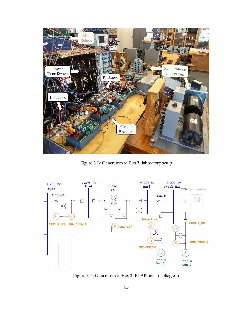
63
Figure 5-3: Generators to Bus 3, laboratory setup
Figure 5-4: Generators to Bus 3, ETAP one line diagram

64
5.2 Load Flow Analysis
Reference [4] states that “the operating characteristics of the laboratory bench
power transformers presented certain difficulties in this project. Due to their construction,
the transformers consistently operate in saturation.” Magnetization current observed in
the hardware implementation of the microgrid also results in greater reactive power,
lower power factor, and overall more losses throughout the system. Energizing the
transformers in the laboratory resulted in an observed magnetizing current of about
150mA each. Protective elements including instrument transformers and relays are
hidden in the analysis of load flow studies.
5.2.1 Case I: Bidirectional System, No Motor and Capacitors
Table 5-1 displays laboratory measured data of the microgrid to gather load flows
throughout the system, provided from another graduate student working on the Microgrid
lab project per reference [14]. In this scenario the excitation voltage and the output power
of the generator is manually adjusted by setting the speed of the prime mover (DC
motor). Each synchronous generator is operating at 100W, 12Var, supplying a total of
200W and 24Var.

65
Table 5-1: System synchronized, no motor, no capacitors [14]
Location
Real
Power
[W]
Current
[A]
Voltage
[V]
Reactive
Power
[VAR]
Apparent
Power
[VA]
Power
Factor
Generator 200 .563 208 24 235 .857
Utility 133.8 .369 207.6 54.6 152.6 .739
Motor 0 0 194 0 0 1
Figure 5-5 provides a load flow comparison of a one-line depicting the apparent
power (VA) and amps (A) flowing throughout the system. All sources of generation are
selected to operate in swing mode. The utility supplies the power flowing from Bus 2 to
Bus 3, and the generators supply the power flowing from Bus 4 to Bus 3. De-energized
elements are grayed out (motor and capacitor).
Figure 5-5: Load Flow, no motor and capacitors

66
In Figure 5-5, the total current supplied to the static loads at Bus 3 is 0.696 A.
However, laboratory tested data in Table 5-1 suggests total current from utility and the
generators supply about 0.932 A. The discrepancies between the two data can be
attributed to transformer magnetizing current and saturation, both of which are not
modeled in ETAP.
Consider Figure 5-6 in which the synchronous generators are instead operated in
Mvar mode, where the user can enter specific values of active and reactive power
generation from the rating page of the synchronous generator models. The utility is still
selected as swing mode, supplying the remaining power and balancing load flow in the
system. We can observe that the power flowing from Bus 4 to Bus 3 from the generators
closely matches that of Table 5-1 of 200 W and 24 Var. However, we have compromised
the remaining power flowing from the utility in this configuration. This is the inherent
limitation of ETAP load flow modeling of non-ideal components largely due to the
transformers drawing additional current throughout the system. Therefore, even if the
generators are modified to supply specific fixed amounts of reactive and active power,
the ETAP model will not accurately represent the hardware representation of the system,
and there will be less total power flowing in the system when compared to laboratory
data.
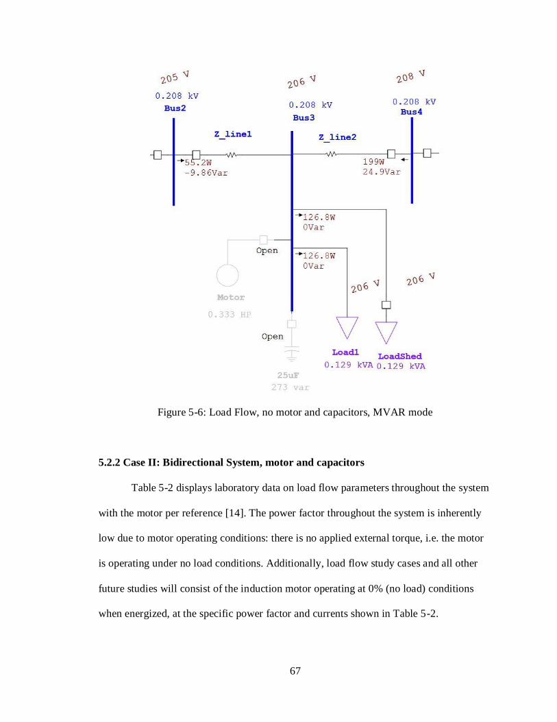
67
Figure 5-6: Load Flow, no motor and capacitors, MVAR mode
5.2.2 Case II: Bidirectional System, motor and capacitors
Table 5-2 displays laboratory data on load flow parameters throughout the system
with the motor per reference [14]. The power factor throughout the system is inherently
low due to motor operating conditions: there is no applied external torque, i.e. the motor
is operating under no load conditions. Additionally, load flow study cases and all other
future studies will consist of the induction motor operating at 0% (no load) conditions
when energized, at the specific power factor and currents shown in Table 5-2.

68
Table 5-2: System Synchronized, with motor, no capacitors [14]
Location
Real
Power
[W]
Current
[A]
Voltage
[V]
Reactive
Power
[VAR]
Apparent
Power
[VA]
Power
Factor
Generator 200 .814 208 214 337 .593
Utility 161 .774 205.7 226 318 .502
Motor 65.7 1.06 173.2 308.3 315.2 .208
The motor modified nameplate characteristics can be seen in Figure 5-7 in ETAP.
The microgrid does not apply external load to the motor, and hence only considers the
case when the motor is turned off or drawing power at no load conditions, with effects of
inrush current negated. The loading column in Figure 5-7 is by default 100% for full load
conditions, but it is instead modified to 0% to more accurately model the system. Hence,
by design the motor is operating in no load conditions. This thesis does not consider
motor dynamic studies, which could be a future project on its own.

69
Figure 5-7: ETAP Induction Motor loading conditions
Figure 5-8 displays the load flow with all generations as swing buses for purposes
of simulation. Power flow between Bus 4 and Bus 3 from the generators and between Bus
2 and Bus 3 from the utility results in a smaller current than that shown in Table 5-2. This
is again due to the inherent limitation of limited reactive power flow in the system as
mentioned in Case 1 of load flow analysis. As a result, Bus 3 voltage is higher than that
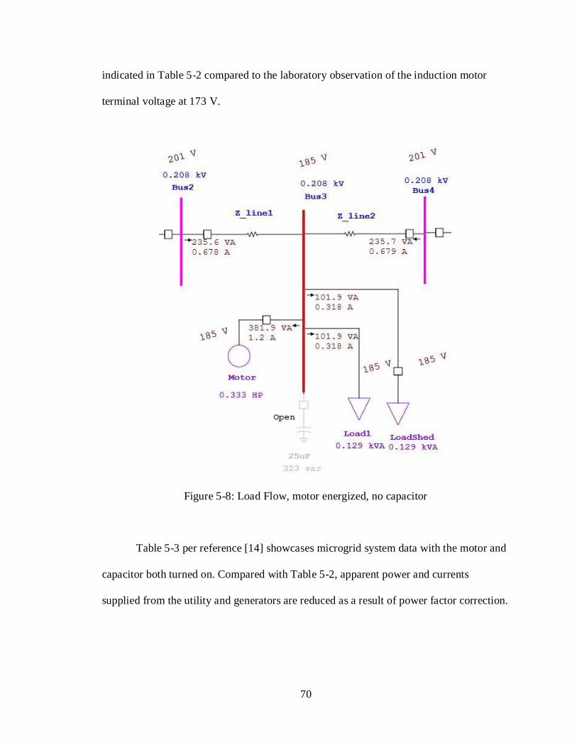
70
indicated in Table 5-2 compared to the laboratory observation of the induction motor
terminal voltage at 173 V.
Figure 5-8: Load Flow, motor energized, no capacitor
Table 5-3 per reference [14] showcases microgrid system data with the motor and
capacitor both turned on. Compared with Table 5-2, apparent power and currents
supplied from the utility and generators are reduced as a result of power factor correction.
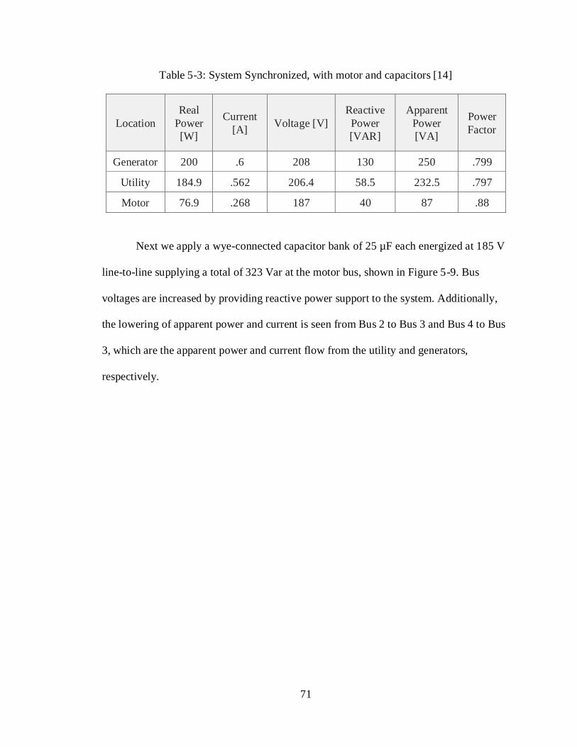
71
Table 5-3: System Synchronized, with motor and capacitors [14]
Location
Real
Power
[W]
Current
[A] Voltage [V]
Reactive
Power
[VAR]
Apparent
Power
[VA]
Power
Factor
Generator 200 .6 208 130 250 .799
Utility 184.9 .562 206.4 58.5 232.5 .797
Motor 76.9 .268 187 40 87 .88
Next we apply a wye-connected capacitor bank of 25 µF each energized at 185 V
line-to-line supplying a total of 323 Var at the motor bus, shown in Figure 5-9. Bus
voltages are increased by providing reactive power support to the system. Additionally,
the lowering of apparent power and current is seen from Bus 2 to Bus 3 and Bus 4 to Bus
3, which are the apparent power and current flow from the utility and generators,
respectively.

72
Figure 5-9: Load Flow, motor and capacitors
5.2.3 Case III: DC Load Flow
Case III of Load Flow analysis considers some of the capabilities and possibilities
of running DC load flow simulations. There is currently no supplementary PV generation
in the microgrid. The future microgrid lab will utilize BP SX 150S Solar Panels rated at
150 W, open circuit voltage of 43.5 V, short circuit current of 4.75 A, maximum power
point operating voltage at 34.5 V, and maximum power point current of 4.35 A. The
inverter to connect to the AC system will be the APsystems 1000W YC-1000 3-phase

73
microverter, whose datasheet can be found per reference [15]. For purposes of
simulations, the Photowatt PV1400 will be used as a model in ETAP for conduction DC
Load Flow, rated at 150 W, maximum power point operating voltage at 33.69 V, and
maximum power point current of 4.45 A, which closely model the BP SX 150S.
Solar panel ratings are provided based on standard test conditions and several
conditions such as solar irradiation, module temperature, angle with respect to the sun,
etc. For purposes of simulations we utilize standard test conditions of 25 degrees Celsius,
and set an irradiance of 200 W/m2 for four PV1400 panels, with a DC load flow shown in
Figure 5-10.
Figure 5-10: DC Load Flow, DC System

74
The inverter can be operated as MVAR controlled AC operation mode, similar to
that of the synchronous generators. With a 95% efficiency, we can specify the AC output
to be 95 W, or any specific fixed amount of the input DC power from the solar panels.
Cable impedance is neglected for purposes of simulation, but can be entered if losses are
needed. This shows the capabilities of the DC load flow: we can investigate different PV
generating parameters and determine output AC power and supply known power to the
microgrid accordingly. Figure 5-11 displays an AC Load Flow taking into account the
DC power supplied by the panels. The generators are heavily relieved from the active
power demanded from the system, supplemented from solar generation. The synchronous
generators instead provide mostly reactive support to the system. The generators and
utility are operating in swing mode, while the inverter is operating in MVAR with fixed
output of 95 W. The motor is turned on, with the capacitor off. The DC_system
subsystem block in Figure 5-11 contains the DC system depicted in Figure 5-10.
Figure 5-11: AC Load Flow, PV generation

75
5.2.4 Load Flow Summary
Cases I-III of Load Flow analysis considered different variations of the
bidirectional microgrid system. In all cases, total power supplied from generation is lower
than the hardware implementation of the microgrid. This is due to inherent limitations of
the Load Flow analysis module which does not consider the effects of transformer
magnetizing current and saturation. Case III also considered the DC Load Flow in which
PV panels were utilized to supplement active power in the system. The future microgrid
can vary the amount of panels based on power demand, and utilize the generator(s) for
reactive power support.
5.3 Short Circuit Analysis
Short circuit analysis will be utilized to determine the contribution of fault
currents from synchronous generators. Per reference [4], the prior microgrid utilized the
utility to supply all the power in the system. Hence, fault contributions from both sides of
the microgrid will essentially be equivalent, with the same relay settings to be discussed
in Section 5.4. Known fault current contribution from the synchronous generators will be
necessary to implement protection and coordination in the current iteration of the
microgrid.
5.3.1 Short Circuit System Validation
Figure 5-12 displays the hardware implementation to extract relevant machine
parameters in the event of a short circuit. SEL-421 is utilized in extracting the fault

76
current from the system. The synchronous generator is originally unloaded, driven by a
DC motor for the prime mover and field excitation by a rheostat producing rated voltage
(208 Vac) and rated speed (1800 rpm). A three-phase fault is suddenly applied on the
terminals of the machine.
Figure 5-12: Three-phase short circuit test, synchronous generator
Figure 5-13 displays the ETAP implementation demonstrating a three-phase short
circuit to an unloaded synchronous generator. The value displayed as 0.002 represents
minimum (30 cycle) short circuit current Arms from the generator, after the asymmetrical

77
component has decayed. Refer to Chapter 4 on a discussion of asymmetrical short circuit
current.
Figure 5-13: ETAP, three-phase short circuit test, synchronous generator
Figure 5-14 displays an oscillogram from an SEL-421 event report showcasing
the generator response to a three-phase short circuit. The peak asymmetrical current is
approximately 10.6 A, corresponding to a 7.5 Arms current. The asymmetrical (dc)
component quickly dies down in less than a cycle and reaches a steady-state peak current
of approximately 2.1 A or 1.5 Arms.

78
Figure 5-14: SEL Oscillogram, three-phase short circuit, synchronous generator
Figure 5-15 illustrates a plot utilizing ETAP transient stability module of a sudden
three-phase short circuit data, showcasing the envelope of the asymmetrical current. The
current in Figure 5-15 is provided in rms values, which is consistent with the hardware
test of approximately 7 Arms asymmetrical peak and 1.5 Arms steady state short circuit. As
will be seen in Section 5.4 this steady short circuit current will be utilized in the
coordination of fault protection.
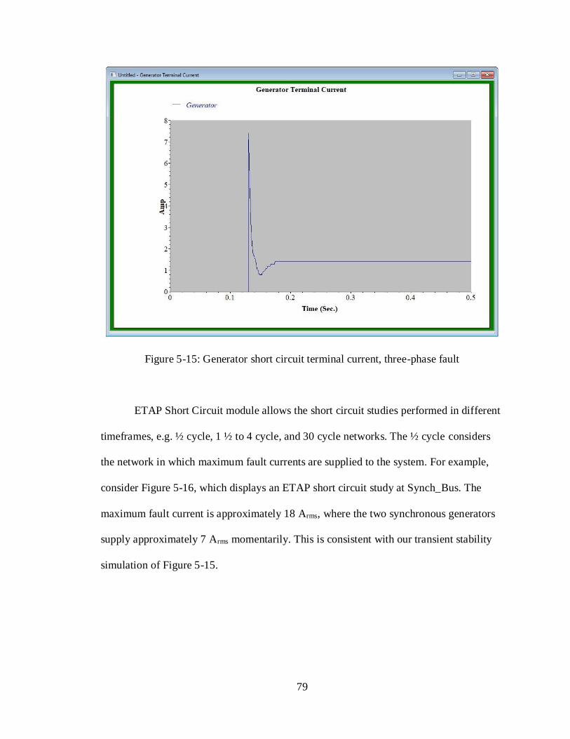
79
Figure 5-15: Generator short circuit terminal current, three-phase fault
ETAP Short Circuit module allows the short circuit studies performed in different
timeframes, e.g. ½ cycle, 1 ½ to 4 cycle, and 30 cycle networks. The ½ cycle considers
the network in which maximum fault currents are supplied to the system. For example,
consider Figure 5-16, which displays an ETAP short circuit study at Synch_Bus. The
maximum fault current is approximately 18 Arms, where the two synchronous generators
supply approximately 7 Arms momentarily. This is consistent with our transient stability
simulation of Figure 5-15.

80
Figure 5-16: Maximum 3-phase SC (1/2 cycle) on generator terminals
Consider Figure 5-17 where the maximum fault current has been decreased from
the generators. The fault at Synch_Bus has a minimum fault current of approximately
0.006 kArms or 6Arms, much lower than maximum simulated of 18 Arms. This is the steady
state asymmetrical short circuit current after the subtransient and transient portions has
decayed.
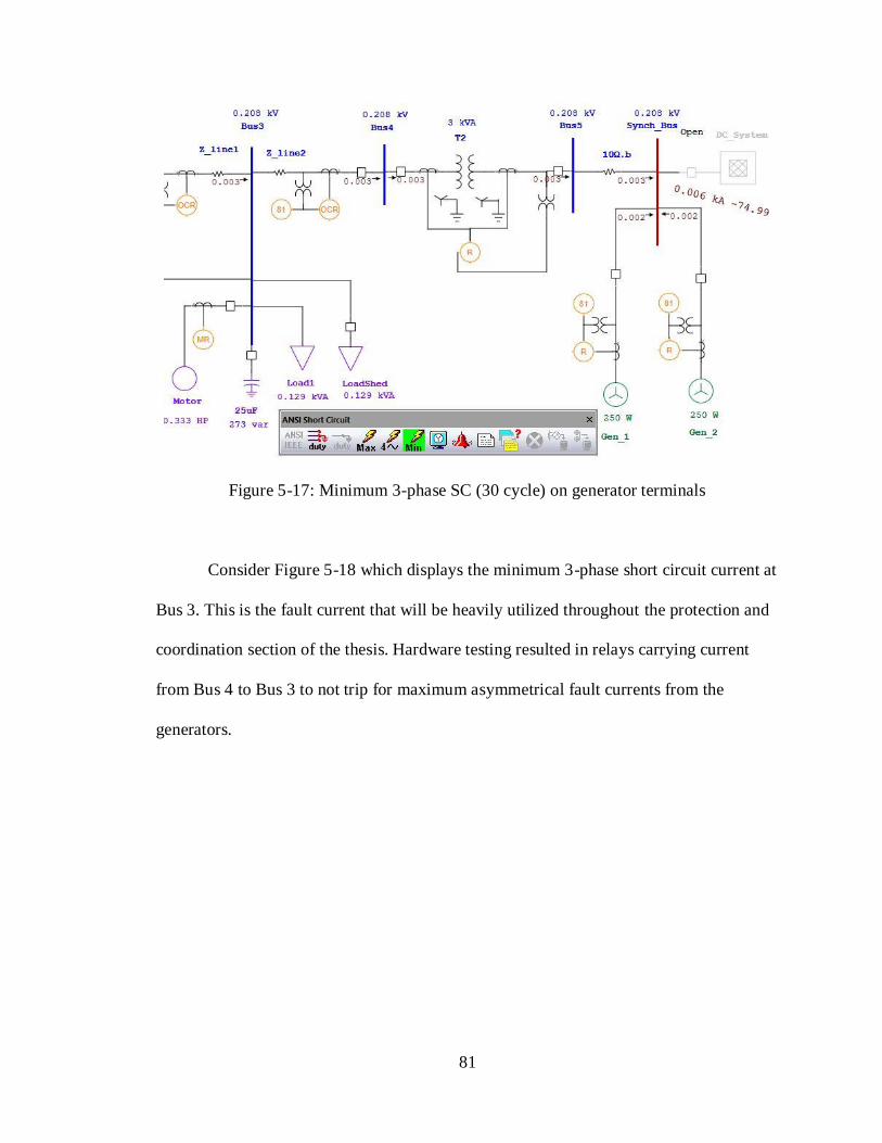
81
Figure 5-17: Minimum 3-phase SC (30 cycle) on generator terminals
Consider Figure 5-18 which displays the minimum 3-phase short circuit current at
Bus 3. This is the fault current that will be heavily utilized throughout the protection and
coordination section of the thesis. Hardware testing resulted in relays carrying current
from Bus 4 to Bus 3 to not trip for maximum asymmetrical fault currents from the
generators.

82
Figure 5-18: Minimum 3-phase SC (30 cycle) on Bus3
Figure 5-19 provides short circuit data for a line-to-line-to-ground fault at Bus 3.
The first row provides the total fault current at Bus 3 due to all sources of generation. The
second row provides short circuit data from Bus 2 to Bus 3, namely the short circuit
contribution from the utility. For example, sequence current I1 of 4 Arms, I2 of 3 Arms,
and I0 of 2 Arms are the positive, negative, and zero sequence currents from the utility,
respectively, due to a double line-to-ground fault at Bus 3. The third row provides short
circuit data from Bus 4 to Bus 3, namely the short circuit contribution from the

83
generators. A complete tabulation of necessary short-circuit date can be found in the
appendix.
Figure 5-19: Double-Line-to-Ground Fault Bus 3, short circuit report
5.3.2 Short Circuit Summary
Short circuit analysis was utilized primarily as a precursor to the protection and
coordination analysis. Maximum and minimum fault current contribution case studies
were conducted, and the advantage of ETAP allows us to fault any bus with any kind of
fault to obtain short circuit data. ETAP provides us to the tools to now be able to
coordinate for faults at any bus by dissecting the positive, negative, and zero sequence
component from the short circuit reports and adjusting relay settings as necessary. In
particular, we are concerned with faults applied at Bus 3, the load bus, since we will
coordinate our protective relays based on faults primarily the motor terminals as will be
presented in Section 5.4.

84
5.4 Protection and Coordination Analysis
We begin our ETAP protection and coordination analysis by considering several
case studies. Case I considers the prior microgrid setup conducted in 2017, and analyzes
an ETAP model with the hardware realization of the system. The following cases then
study the current iteration of the microgrid with added synchronous generators and
relays.
5.4.1 Case I: Protection System Validation
Case I considers the ETAP model of the previous microgrid and compares its
protection coordination results with the hardware implementation of the microgrid for
purposes of system validation and accuracy. Figure 5-20 models and displays a portion of
the bidirectional system of the previous iteration of the microgrid. The bus is fully loaded
with the induction motor and static loads drawing power. A double line-to-ground fault is
suddenly applied on the terminals of the induction motor at Bus 3. Figure 5-20 displays
the sequence-of-operation (SQOP) utilizing ETAP’s STAR protection module, indicating
the order of operation in which circuit breakers trip due to a fault applied at Bus 3. An
‘X’ next to a number on the circuit breaker shows the tripping of circuit breakers in order
due to a line-to-line-to-ground fault. Notice that this adheres to coordination criteria:
circuit breakers closest to the fault trip, followed by circuit breakers upstream to the fault.
Generation consists of the utility at 240 Vac to the left and right of the one-line, not
shown in Figure 5-20.

85
Figure 5-20: SQOP, Double Line-to-Ground Fault, prior microgrid
Figure 5-21 displays the SQOP viewer, showcasing a more analytical view of the
tripping of circuit breakers. The time (in ms) column indicates the moment at which
certain protective elements have asserted different commands, T1 (ms) indicates the
operating time of the device, and the condition column indicates the reasoning behind the
operation of protective elements. For example, at time 85.2 ms SEL-311L-1’s negative
inverse overcurrent (51Q) element asserts trip signals to circuit breaker CB2-3. At time
119 ms, CB2-3 opens the line within two cycles (T1 = 33.3 ms), providing secondary
protection for a double line-to-ground fault at the induction motor in case primary
protection from SEL-710 misoperates or fails.

86
Figure 5-21: SQOP Report, Double Line-to-Ground, prior microgrid
Consider Table 5-4 which is tabulated per reference [4] of the previous microgrid
configuration indicating the system tripping time for the same fault in Figure 5-20. The
ETAP model showcases a very accurate tripping time compared to the previous
microgrid. For example, SEL-587 trips at time 109 ms in Table 5-4, compared to 112 ms
in Figure 5-21. Imbalances in tripping times shown in Table 5-4 could be attributed to
slight imbalances in the microgrid, differences in pre-fault voltages, and system
impedances, but ultimately the ETAP model indicates a very accurate response to the
system for the double line-to-ground fault.

87
Table 5-4: Bidrectional System Tripping for a Double-Line-to-Ground Fault [4]
TIME
DELTA
(mSEC)
SEL RELAY
DEVICE
ASSERTED
ELEMENTS COMMENT
7 710 TRIP Instantaneous Trip
80 311L - LINE 2 51QT, TRIP Timeout and Trip
84 311L - LINE 1 51QT, TRIP Timeout and Trip
109 587 51Q2T, TRIP Timeout and Trip
114 387E 51Q2T, TRIP Timeout and Trip
Table 5-5 provides settings for both the hardware implementation as well as
settings implemented in ETAP for negative-sequence time overcurrent protection (and
motor protection) for the prior iteration of the microgrid. In particular, the negative
sequence elements are identical for both hardware and software implementations for
system validation.

88
Table 5-5: Negative sequence time overcurrent settings, prior microgrid
Relay ID Device
Function
Trip
Element Curve
OCR (50, 51), OLR (49,
Acc.)
Pickup
(A)
Prim.
Amps
(A)
Time
Dial
Setting
SEL-387E Overcurrent Negative Sequence
U1- U.S. Moderately
Inverse 0.500 0.500 0.550
SEL-710 Overload Overload
Phase 2.280 2.00
SEL-311L-1 Overcurrent Negative Sequence
U1 - U.S. Moderately
Inverse
0.250 0.250 0.500
SEL-311L-2 Overcurrent Negative Sequence
U1 - U.S. Moderately
Inverse 0.250 0.250 0.500
SEL-587 Overcurrent Negative Sequence
U1 - U.S.
Moderately Inverse
0.500 0.500 0.550
Figure 5-22 demonstrates a time-current curve (TCC) of a line-to-line-to-ground
fault at the terminals of the induction motor, as indicated in Figure 5-20. The vertical
dashed red arrow indicates a normalized fault current of 1 per unit, corresponding to 10.8
Arms fault current. The time difference shown in blue of 0.0269 seconds (26.9 ms) is
indicative of the delay between upstream relays. SEL-710’s instantaneous phase
overcurrent protection first detects and trips the nearby circuit breaker on the motor
terminals. This is observed by SEL-710’s instantaneous vertical overcurrent curve having
a pickup setting less than the fault current to the right. The overlapping pair of negative
sequence time overcurrent curves for SEL-311L-1 and SEL-311L-2, as well as SEL-587
and SEL-387E are due to identical relay settings tabulated in Table 5-5.

89
Figure 5-22 illustrates an example of the following design criteria for system
protection outline in Chapter 4: reliability, selectivity, speed, economy, and simplicity
[11]. Glover suggests that “Precise determine of relay operating times is complicated by
several factors, including CT error, dc offset component of fault current, and relay
overtravel. Therefore, typical coordination time intervals from 0.2 to 0.5 seconds are
selected to account for these factors in most practical applications” [11]. The time
difference of 26.9 ms in Figure 5-22 can be argued to be too low of a coordination time
interval between secondary and tertiary protection in the prior iteration of the microgrid.
Circuit breakers in the Cal Poly microgrid clear the fault within 33 ms (two cycles),
therefore this protection scheme can be improved by allowing a greater time delay added
to both SEL-311’s as well as SEL-587 and SEL-387E negative sequence settings.
Although this protection scheme was verified in the prior implementation of the
microgrid, the time margin between relay operating times may be susceptible for false
tripping, and illustrates the compromise of relay selectivity in favor of relay speed.

90
Figure 5-22: TCC Bidirectional Relay Coordination, prior microgrid
Figure 5-23 shows a modified protection scheme for a double line-to-ground fault
at the terminals of the induction motor for the prior microgrid. Greater selectivity is
achieved by implementing adequate time delay between secondary and tertiary
protection. Time difference t1 of 0.334 seconds is the time margin for SEL-311L-1 and
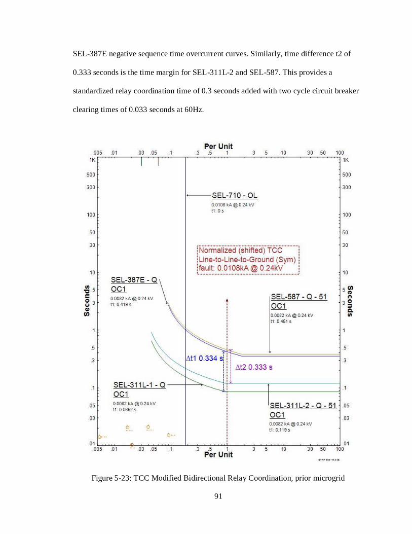
91
SEL-387E negative sequence time overcurrent curves. Similarly, time difference t2 of
0.333 seconds is the time margin for SEL-311L-2 and SEL-587. This provides a
standardized relay coordination time of 0.3 seconds added with two cycle circuit breaker
clearing times of 0.033 seconds at 60Hz.
Figure 5-23: TCC Modified Bidirectional Relay Coordination, prior microgrid

92
Table 5-6 provides settings implemented in ETAP for negative-sequence time
overcurrent protection for the modified prior iteration of the bidirectional system
illustrated in Figure 5-23. Comparisons can be made with Table 5-5 to observe the
variations in time delay. For example, SEL-311L-2 was modified from a time delay of
0.5 to 0.7 and SEL-587 from 0.55 to 2.220 for purposes of illustrating a modified
protection scheme with added selectivity instead of speed.
Table 5-6: Negative sequence time overcurrent settings, modified prior microgrid
Relay ID Device
Function
Trip
Element Curve
OCR (50, 51), OLR (49,
Acc.)
Pickup (A)
Prim. Amps
(A)
Time Dial
Setting
SEL-710 Overload Overload
Phase 2.280 2.00
SEL-311L-1 Overcurrent Negative
Sequence
U1 - U.S.
Moderately Inverse 0.250 0.250 0.500
SEL-311L-2 Overcurrent Negative
Sequence
U1 - U.S.
Moderately Inverse 0.250 0.250 0.700
SEL-387E Overcurrent Negative Sequence
U1- U.S. Moderately Inverse
0.500 0.500 2.060
SEL-587 Overcurrent Negative
Sequence
U1 - U.S.
Moderately Inverse 0.500 0.500 2.220
Figure 5-24 displays the SQOP viewer for the modified protection scheme. In this
scenario relay trip signals are slower than the prior microgrid, with added selectivity
gained. Ultimately, protection is not an exact science and there is no ideal right answer in

93
incorporating relay settings—there are tradeoffs that must be taken into account. For
example, we will investigate the detriment of having slower relay fault clearing speeds in
transient stability case I.
Figure 5-24: SQOP viewer, DLG fault improved selectivity
Consider Figure 5-25 displaying an SEL oscillogram per reference [4] showcasing
differential protection of the prior microgrid. In this illustration, “the restrained
differential element (87R) on the SEL-387E asserts approximately 2 cycles after fault
inception, whereupon the relay trips its circuit breakers on Bus 1 and Bus 2 to clear the
fault” [4].
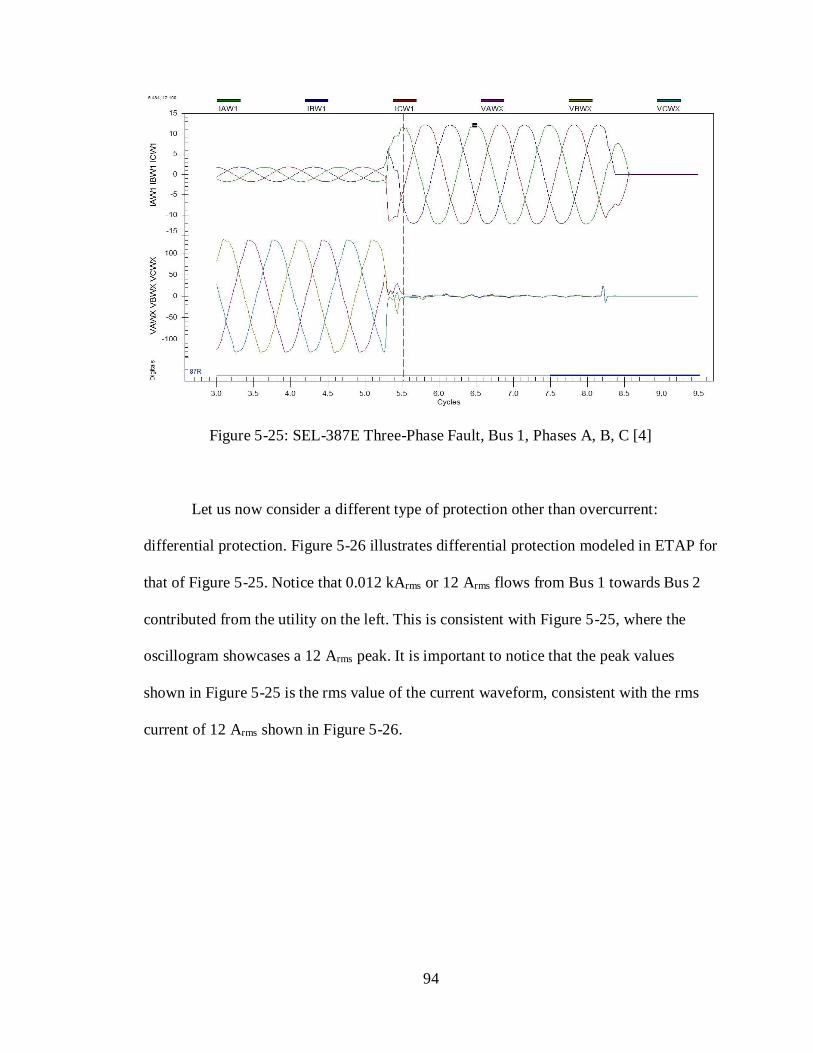
94
Figure 5-25: SEL-387E Three-Phase Fault, Bus 1, Phases A, B, C [4]
Let us now consider a different type of protection other than overcurrent:
differential protection. Figure 5-26 illustrates differential protection modeled in ETAP for
that of Figure 5-25. Notice that 0.012 kArms or 12 Arms flows from Bus 1 towards Bus 2
contributed from the utility on the left. This is consistent with Figure 5-25, where the
oscillogram showcases a 12 Arms peak. It is important to notice that the peak values
shown in Figure 5-25 is the rms value of the current waveform, consistent with the rms
current of 12 Arms shown in Figure 5-26.
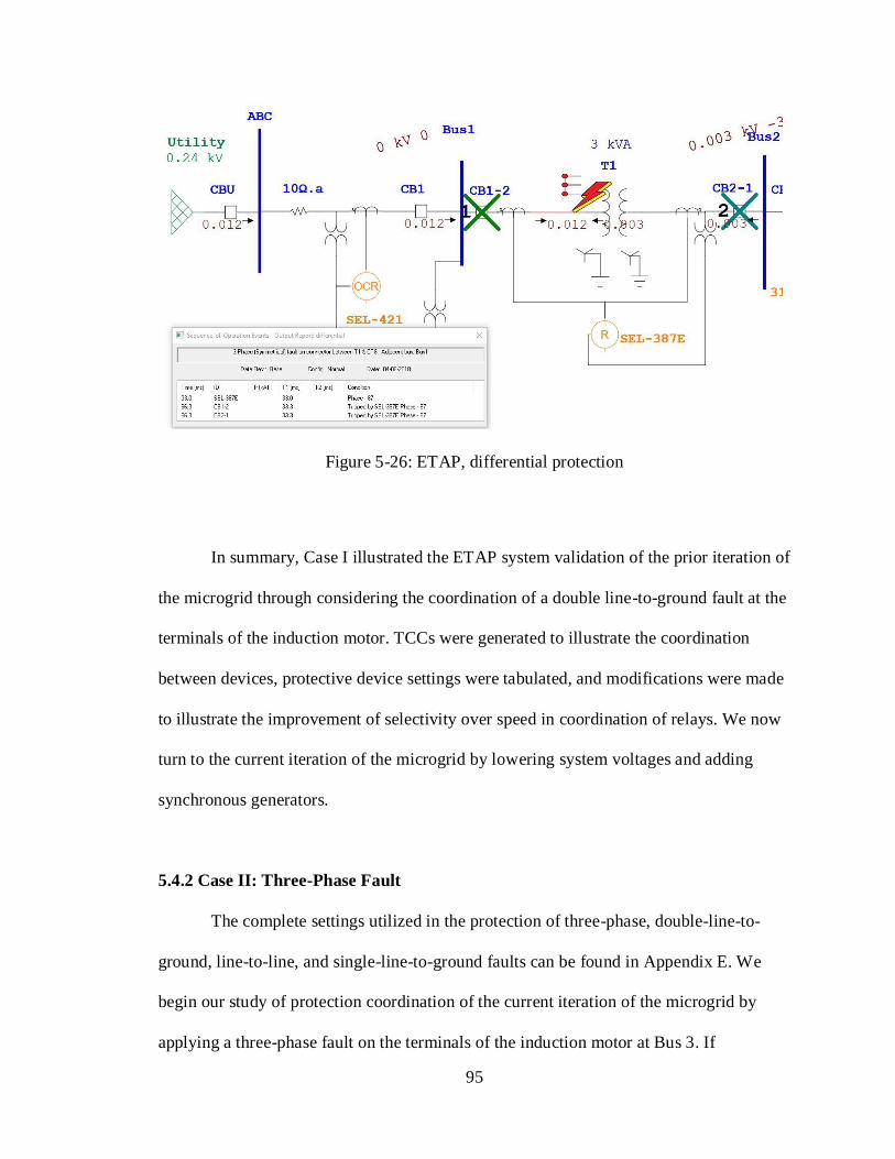
95
Figure 5-26: ETAP, differential protection
In summary, Case I illustrated the ETAP system validation of the prior iteration of
the microgrid through considering the coordination of a double line-to-ground fault at the
terminals of the induction motor. TCCs were generated to illustrate the coordination
between devices, protective device settings were tabulated, and modifications were made
to illustrate the improvement of selectivity over speed in coordination of relays. We now
turn to the current iteration of the microgrid by lowering system voltages and adding
synchronous generators.
5.4.2 Case II: Three-Phase Fault
The complete settings utilized in the protection of three-phase, double-line-to-
ground, line-to-line, and single-line-to-ground faults can be found in Appendix E. We
begin our study of protection coordination of the current iteration of the microgrid by
applying a three-phase fault on the terminals of the induction motor at Bus 3. If

96
coordinated correctly, the protective devices closest to the fault should open first
followed by breakers upstream to the fault. The symmetrical components of a balanced
three-phase fault result in only positive sequence components, and therefore phase
overcurrent protection is utilized for this case. SEL-710 first clears the fault utilizing
phase instantaneous overcurrent protection (ANSI 50P). Secondary protection is
implemented utilizing phase time-overcurrent protection (51PT) for SEL311L-1 and
SEL311L-2. Tertiary protection is implemented utilizing 51PT settings for SEL-387E
and SEL-587. Figure 5-27 displays the sequence-of-events (SQOP) of circuit breakers
tripping in order indicated by a number beside an ‘X’ for a three phase fault on the
terminals of the induction motor.
Figure 5-27: SQOP, Three-Phase Fault, Motor Terminals

97
The opening of circuit breakers can be investigated more analytically through
ETAP’s sequence-of-operation (SQOP) event viewer, shown in Figure 5-28. At time t = 0
sec, a three-phase fault is applied onto the terminals of the induction motor. SEL-710’s
instantaneous overcurrent protection detects and opens the nearest circuit breaker, CBM.
Breaker CBM operates in 33.3 ms, clearing the fault in two cycles.
Figure 5-28: SQOP Events, three-phase fault motor terminals
Consider Figure 5-29 which illustrates a time-current curve (TCC) of a three-
phase fault injected on the terminals of the induction motor. The vertical red dashed
arrows indicate the approximate contribution to the fault currents from both the utility
and the synchronous generators. Notice that phase time-inverse overcurrent (51P) curves
for both SEL-311L-2 and SEL-587 are shifted towards the left. This is necessary and
indicative of lower pickup settings for the aforementioned relays due to being in a path
with smaller fault currents from the generators. However, SEL-387E and SEL-311L 51P

98
curves are shifted towards the right, due to higher pickup settings a result of being on the
path sustaining fault current from the utility.
Figure 5-29: Three-Phase Fault, Motor Terminals, TCC

99
5.4.3 Case III: Single-Line-to-Ground
A single-line-to-ground fault is applied on the terminals of the motor.
Decomposition of the fault current results in positive, negative, and zero sequence
components. SEL-710 first clears the fault utilizing definite-time residual overcurrent
element (50G). SEL-311L-1 and SEL-311L-2 utilize inverse-time negative sequence
elements (51Q) providing secondary backup protection. Similarly, SEL-587 and SEL-
387E utilize 51Q to provide tertiary backup protection. Figure 5-30 displays the
sequence-of-events (SQOP) of circuit breakers tripping in order indicated by a number
beside an ‘X’ for a single-line-to-ground fault on the terminals of the induction motor.
Additionally, currents shown in Figure 5-30 display the 3Io ground fault current. This
case proves to be the anomaly between all the different short circuit tests, with higher
single-line-to-ground fault current in the system. Generator grounding schemes could
contribute to the higher sustained fault current, and can be modified in ETAP to more
accurately model a smaller ground fault current as observed in laboratory. However,
tripping still adheres to coordination criteria. Figure 5-31 provides the SQOP events for
the operation of protective devices.

100
Figure 5-30: SQOP, SLG, Motor Terminals
Figure 5-31: SQOP Events, SLG, Motor Terminals
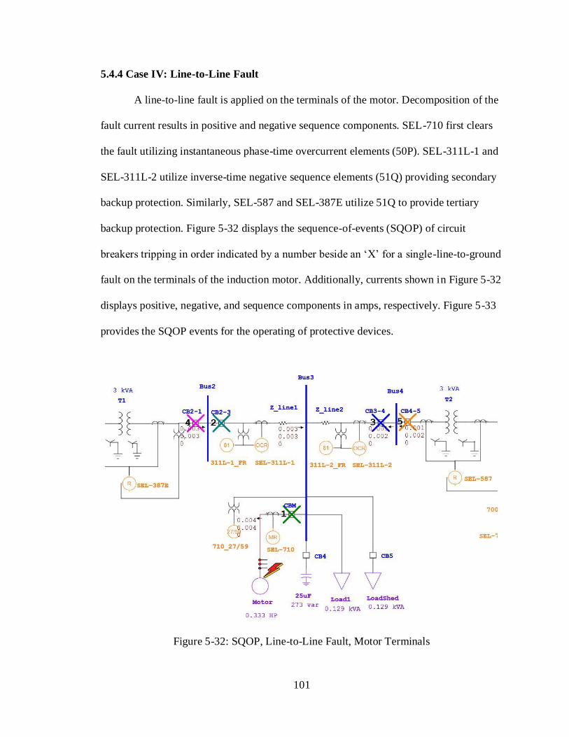
101
5.4.4 Case IV: Line-to-Line Fault
A line-to-line fault is applied on the terminals of the motor. Decomposition of the
fault current results in positive and negative sequence components. SEL-710 first clears
the fault utilizing instantaneous phase-time overcurrent elements (50P). SEL-311L-1 and
SEL-311L-2 utilize inverse-time negative sequence elements (51Q) providing secondary
backup protection. Similarly, SEL-587 and SEL-387E utilize 51Q to provide tertiary
backup protection. Figure 5-32 displays the sequence-of-events (SQOP) of circuit
breakers tripping in order indicated by a number beside an ‘X’ for a single-line-to-ground
fault on the terminals of the induction motor. Additionally, currents shown in Figure 5-32
displays positive, negative, and sequence components in amps, respectively. Figure 5-33
provides the SQOP events for the operating of protective devices.
Figure 5-32: SQOP, Line-to-Line Fault, Motor Terminals

102
Figure 5-33: SQOP Events, Line-to-Line Fault, Motor Terminals
5.4.5 Case V: Line-to-Line-to-Ground Fault
A line-to-line fault is applied on the terminals of the motor. Decomposition of the
fault current results in positive, negative, and zero sequence components. SEL-710 first
clears the fault utilizing instantaneous phase-time overcurrent elements (50P). SEL-311L-
1 and SEL-311L-2 utilize inverse-time negative sequence elements (51Q) providing
secondary backup protection. Similarly, SEL-587 and SEL-387E utilize 51Q to provide
tertiary backup protection. Figure 5-34 displays the sequence-of-events (SQOP) of circuit
breakers tripping in order indicated by a number beside an ‘X’ for a single-line-to-ground
fault on the terminals of the induction motor. Additionally, currents shown in Figure 5-34
displays positive, negative, and sequence components in amps, respectively. Figure 5-35
provides the SQOP events for the operating of protective devices.

103
Figure 5-34: SQOP, Double Line-to-Ground, Motor Terminals
Figure 5-35: SQOP Events, Double Line-to-Ground, Motor Terminals

104
5.4.6 Case VI: Three-Phase Fault, SEL-421
The SEL-421 is utilized in the microgrid for synchronization purposes with the
utility. Additionally, the SEL-421 will be utilized for overcurrent protection. Figure 5-36
shows a one-line of a three-phase fault applied at Bus 2. The microgrid is energized from
utility only, two static loads are energized, and overcurrent protection from SEL-387E
and SEL-311L-1 is bypassed in the hardware test as well as in ETAP. The three-phase
fault at Bus 2 is detected from SEL-421 at time t = 397 ms from the SQOP in ETAP, and
asserts trip commands to circuit breaker CB1 at time t = 430 ms.
Figure 5-36: SEL-421 test, three-phase fault Bus 2
Figure 5-37 displays event data tested in lab from the SEL-421 for a current
senior design project student per reference [16], equivalent to the system configuration
displayed in the one-line in Figure 5-36. The event data suggests a pickup time of
approximately 458 ms, which is greater than the pickup time of 397 ms from ETAP.

105
SEL-421 event data suggests a slightly lower three-phase fault current of approximately
10.5 Arms (15 Apeak), with respect to nearly 12 Arms observed in ETAP. Variations in
three-phase fault current can be attributed to greater impedances and lower pre-fault
voltages observed in the laboratory test. SEL-421 phase time overcurrent settings utilize a
U1 – Moderately inverse curve type with a pickup setting of 4.5 A and time dial setting
of 0.7.
Figure 5-37: SEL-421 three-phase SC test, Bus 2
5.4.7 Protection and Coordination Summary
ETAP was successfully used to implement the testing of protection and
coordination for both the prior and current iterations of the microgrid. Relay settings
implemented in the section as well as shown in appendix B are settings that are both

106
implemented in the laboratory as well as in ETAP, indicating a successful replication of
relay coordination. Protection and coordination analysis allows users to evaluate different
fault currents flowing throughout the system and implement protection as needed.
Although protection and coordination were primarily conducted on Bus 3, one can
choose to fault a separate bus as shown in Case I and implement protection as necessary,
such as Bus 2 in Case VI. Additional protection schemes such as directional and distance
can be complemented in conjunction of overcurrent protection to protect every section of
the microgrid. For example, the SEL-311L has capabilities of directional overcurrent
protection (ANSI 67) to detect faults flowing opposite to the assumed nominal direction
of current flow. The example studied in Case VI can be extended to include the
bidirectional system with synchronous generators. SEL-311L-1 can implement
directional protection in both laboratory as well as ETAP to coordinate for faults at Bus
2. Of special concern is the relatively low fault current contributed from the synchronous
generators, which will become an issue if the microgrid becomes more heavily loaded;
thus, becoming susceptible to false trips on nominal loading conditions.
5.5 Transient Stability Analysis
Transient stability analysis will be conducted primarily to observe the response of
synchronous generators. These simulations mainly are theoretically based, and not tested
in laboratory. Hence the purpose of this section is to provide insights for the future
microgrid team of transient stability issues that may occur and possible improvements
throughout the cases. Interested readers may refer to Chapter 4 for a review on an
elementary study of power system transient stability.

107
5.5.1 Case I: Faults
The study of protection and coordination will be extended to observe the response
of synchronous generators to faults. There are inherent limitations of transient stability
studies that result in difficulties obtaining accurate results. From the swing equation
discussed in Chapter 4, the rotational inertia constant of a machine H will largely
determine if generators retain stability. Per reference [8], Kundur provides typical values
of H, given in per unit MW·s per MVA shown in Table 5-7.
Table 5-7. Typical values of H, thermal and hydraulic generating units [8]
Type of generating unit Per Unit Inertia Constant, H
(MW·s/MVA)
Thermal unit
(a) 3600 r/min (2-pole)
(b) 1800 r/min (4-pole)
2 to 6.0
4.0 to 10.0
Hydraulic unit 2.0 to 4.0
Kundur also provides another way of interpreting machine inertia constant H by
defining “TM as the time required for rated torque to accelerate the rotor from standstill to
rated speed” [8], resulting in equation 5-1 describing:
𝑇𝑀 = 2𝐻 [s] (5-1)
where “TM is called the mechanical starting time” [8]. For example, for an 1800 r/min (4-
pole) thermal unit of H = 4.0 MW·s/MVA, mechanical starting time would be 8 seconds
per equation 5-1.
However, the issue resulted from inherently very low rotational inertia presents in
synchronous machinery used in the microgrid. ETAP is originally designed for industrial
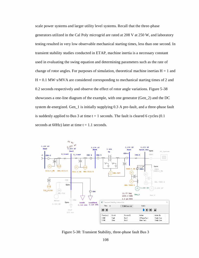
108
scale power systems and larger utility level systems. Recall that the three-phase
generators utilized in the Cal Poly microgrid are rated at 208 V at 250 W, and laboratory
testing resulted in very low observable mechanical starting times, less than one second. In
transient stability studies conducted in ETAP, machine inertia is a necessary constant
used in evaluating the swing equation and determining parameters such as the rate of
change of rotor angles. For purposes of simulation, theoretical machine inertias H = 1 and
H = 0.1 MW·s/MVA are considered corresponding to mechanical starting times of 2 and
0.2 seconds respectively and observe the effect of rotor angle variations. Figure 5-38
showcases a one-line diagram of the example, with one generator (Gen_2) and the DC
system de-energized. Gen_1 is initially supplying 0.3 A pre-fault, and a three-phase fault
is suddenly applied to Bus 3 at time t = 1 seconds. The fault is cleared 6 cycles (0.1
seconds at 60Hz) later at time t = 1.1 seconds.
Figure 5-38: Transient Stability, three-phase fault Bus 3

109
Figure 5-39: Rotor angle response, H = 1 MW·s/MVA, 6 cycle clear
Figure 5-39 displays the rotor angle response of the generator with respect to the
applied and clearing of the fault for a machine inertia constant H of 1.0 MW·s/MVA. The
generator internal rotor angle is approximately 12 degrees, shooting to a maximum of
about 27 degrees as the fault is initiated, and decays to a new operating angle after the
fault has cleared. Notice that although the fault is cleared 6 cycles later at time t = 1.1
seconds, the machine cannot stabilize instantaneously to a constant rotor angle as the
rotor accelerates and decelerates from 1800 rpm, observed as oscillations in the rotor
angle.
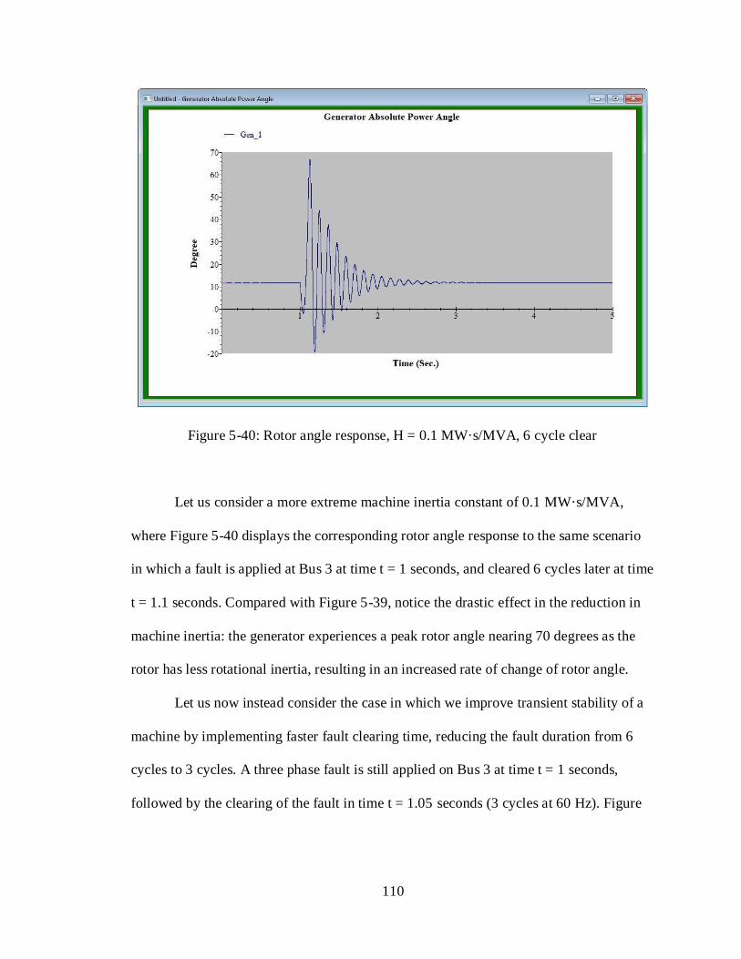
110
Figure 5-40: Rotor angle response, H = 0.1 MW·s/MVA, 6 cycle clear
Let us consider a more extreme machine inertia constant of 0.1 MW·s/MVA,
where Figure 5-40 displays the corresponding rotor angle response to the same scenario
in which a fault is applied at Bus 3 at time t = 1 seconds, and cleared 6 cycles later at time
t = 1.1 seconds. Compared with Figure 5-39, notice the drastic effect in the reduction in
machine inertia: the generator experiences a peak rotor angle nearing 70 degrees as the
rotor has less rotational inertia, resulting in an increased rate of change of rotor angle.
Let us now instead consider the case in which we improve transient stability of a
machine by implementing faster fault clearing time, reducing the fault duration from 6
cycles to 3 cycles. A three phase fault is still applied on Bus 3 at time t = 1 seconds,
followed by the clearing of the fault in time t = 1.05 seconds (3 cycles at 60 Hz). Figure

111
5-41 displays the faster clearing of the fault at time t = 1.05 seconds, with a much lower
peak rotor angle when compared to Figure 5-40.
Figure 5-41: Rotor angle response, H = 0.1 MW·s/MVA, 3 cycle clear
Figure 5-42 displays the terminal current response for the scenario shown in
Figure 5-41. Notice the asymmetrical short circuit current decaying to a steady state value
quickly. This is similar to the expected response of the generator terminal current
considered in Section 5.3. However, the peak asymmetrical current reaches about 3.5
Arms instead of over 7 Arms as tested and simulated in Section 5.3. This is largely due to
the fault not initiated on the terminals of the generator but instead applied further
downstream at Bus 3, with added impedance seen from the generator terminals.

112
Figure 5-42: Generator terminal current response, H = 0.1 MW·s/MVA, 3 cycle clear
Lastly, Figure 5-43 displays the generator speed response due to a three-phase
fault applied at Bus 3 and cleared within 3 cycles with an inertia constant H of 1.0
MW·s/MVA. Notice the generator operating at steady state 1800 rpm prior to the fault at
time t = 1 seconds as expected. Once the fault is initiated, electrical power output
decreases, and hence the rotor accelerates greater than 1800 rpm. As the fault is cleared at
time t = 1.05 seconds, the rotor speed still oscillates between 1800 rpm, constantly
supplying or absorbing kinetic energy as the generator attempts to stabilize back to 1800
rpm.
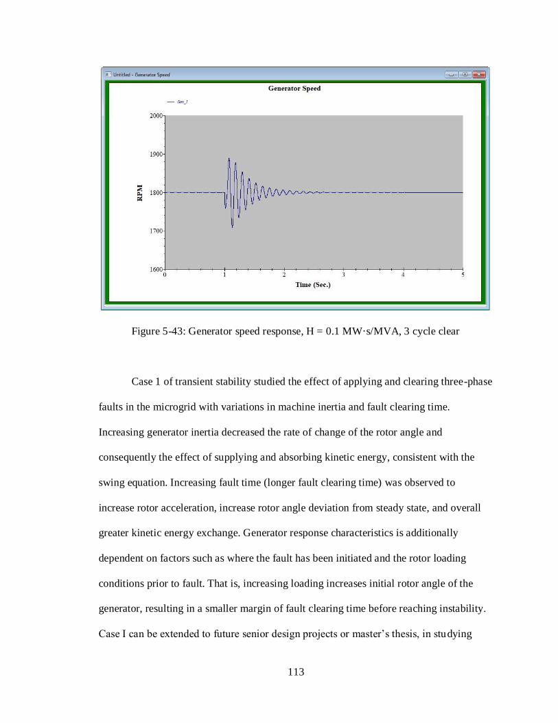
113
Figure 5-43: Generator speed response, H = 0.1 MW·s/MVA, 3 cycle clear
Case 1 of transient stability studied the effect of applying and clearing three-phase
faults in the microgrid with variations in machine inertia and fault clearing time.
Increasing generator inertia decreased the rate of change of the rotor angle and
consequently the effect of supplying and absorbing kinetic energy, consistent with the
swing equation. Increasing fault time (longer fault clearing time) was observed to
increase rotor acceleration, increase rotor angle deviation from steady state, and overall
greater kinetic energy exchange. Generator response characteristics is additionally
dependent on factors such as where the fault has been initiated and the rotor loading
conditions prior to fault. That is, increasing loading increases initial rotor angle of the
generator, resulting in a smaller margin of fault clearing time before reaching instability.
Case I can be extended to future senior design projects or master’s thesis, in studying

114
purely the effect of generator response due to different faulted scenarios. Lastly, Case I
reiterates the importance of inertia: increasing the amount of generation from sources
other than generators reduces system overall inertia and compromises stability. There is
no rotational inertia associated with photovoltaics or battery storage systems, which could
adversely affect stability of the system.
5.5.2 Case II: Islanding
This case investigates the generator response to islanding from utility utilizing the
transient stability analysis module in ETAP. We consider the microgrid in a state in
which power feeds two static loads, and suddenly islanded at time t = 1.0 seconds. We
consider only the utility and one generator as sources of generation. The generators are
assumed to have an inertia constant H of 1.0 MW·s/MVA. Per swing equation of 4-8,
electrical demand is suddenly increased, and a deceleration of machines should be
observed. Figure 5-44 shows the speed response of the generator.
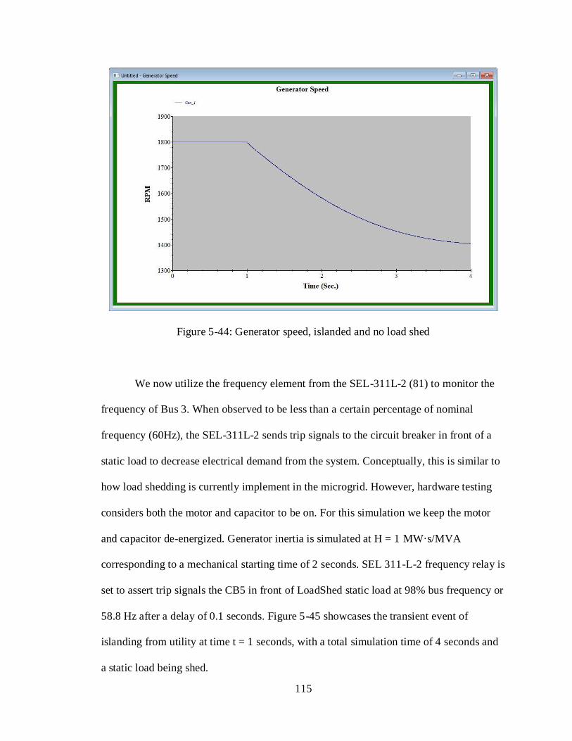
115
Figure 5-44: Generator speed, islanded and no load shed
We now utilize the frequency element from the SEL-311L-2 (81) to monitor the
frequency of Bus 3. When observed to be less than a certain percentage of nominal
frequency (60Hz), the SEL-311L-2 sends trip signals to the circuit breaker in front of a
static load to decrease electrical demand from the system. Conceptually, this is similar to
how load shedding is currently implement in the microgrid. However, hardware testing
considers both the motor and capacitor to be on. For this simulation we keep the motor
and capacitor de-energized. Generator inertia is simulated at H = 1 MW·s/MVA
corresponding to a mechanical starting time of 2 seconds. SEL 311-L-2 frequency relay is
set to assert trip signals the CB5 in front of LoadShed static load at 98% bus frequency or
58.8 Hz after a delay of 0.1 seconds. Figure 5-45 showcases the transient event of
islanding from utility at time t = 1 seconds, with a total simulation time of 4 seconds and
a static load being shed.

116
Figure 5-45: Islanded, Load Shed
Figure 5-46 shows the frequency in percent nominal (60%) at Bus 3 after the
microgrid has been islanded at time t = 1 seconds. As the frequency drops below 98%
(58.8 Hz), the relay asserts trip signals to shed load 0.1 seconds later at time t = 1.269
seconds. In response, the frequency begins to increase as generator speed increases.

117
Figure 5-46: Bus 3 frequency, islanding load shed
Figure 5-47 displays the generator speed response as load is shed from the
islanding event. Compared to Figure 5-44, the generator speed increases due to the
lowering of electrical demand. However, the generator does not return to nominal
operating speed (1800 rpm). Generator rpm can be improved with faster load shedding
times, increased system inertia, or supplemented generation.
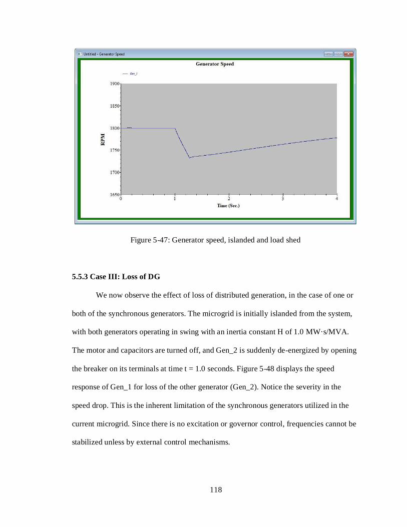
118
Figure 5-47: Generator speed, islanded and load shed
5.5.3 Case III: Loss of DG
We now observe the effect of loss of distributed generation, in the case of one or
both of the synchronous generators. The microgrid is initially islanded from the system,
with both generators operating in swing with an inertia constant H of 1.0 MW·s/MVA.
The motor and capacitors are turned off, and Gen_2 is suddenly de-energized by opening
the breaker on its terminals at time t = 1.0 seconds. Figure 5-48 displays the speed
response of Gen_1 for loss of the other generator (Gen_2). Notice the severity in the
speed drop. This is the inherent limitation of the synchronous generators utilized in the
current microgrid. Since there is no excitation or governor control, frequencies cannot be
stabilized unless by external control mechanisms.

119
Figure 5-48: Generator speed response, loss of DG
Figure 5-49 shows the generator governor tab with sample data available for a
ST1 Single-Reheat Steam-Turbine governor-turbine system. The objective is purely to
showcase the application of a governor control system thereby providing insight for
methods in improving transient stability in the microgrid.

120
Figure 5-49: ST1 Governor sample data
Table 5-8 consists of parameter definitions for the data shown in Figure 5-49,
taken from ETAP Help 16.0. Recall that the prime mover utilized in the hardware
implementation of the microgrid is a DC motor, and hence will not have several
parameters listen in Table 5-8. Nonetheless, these constants are utilized for demonstrating
generator response with governor control.

121
Table 5-8: Single-Reheat Steam-Turbine (ST1) parameters and definitions [10]
Parameter Definition Unit
Mode Droop or Isoch
Droop Steady-state speed droop %
Fhp ( Shaft capacity ahead of reheater)/(Total shaft
capacity ) p.u.
Pmax Maximum shaft power MW
Pmin Minimum shaft power MW
Tc Control Amplifier (servomotor) time constant seconds
Tch Steam time constant seconds
Tdrp Load sensor time constant seconds
Tsr Speed relay time constant seconds
The effect of loss of DG and the speed response of the remaining energized
generator will be observed next. Figure 5-50 displays the speed response of the generator
utilizing the governor control to adjust the speed. This showcases the advantages of
implementing a control scheme to stabilize system frequencies during disturbances.
Several considerations have to take into account into designing a control scheme for
governor control, including the inherently low time constants and low inertia associated
with the synchronous generators utilized in the microgrid.
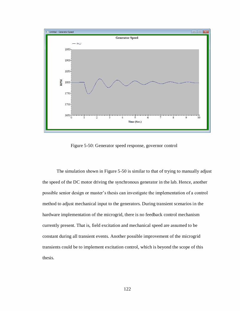
122
Figure 5-50: Generator speed response, governor control
The simulation shown in Figure 5-50 is similar to that of trying to manually adjust
the speed of the DC motor driving the synchronous generator in the lab. Hence, another
possible senior design or master’s thesis can investigate the implementation of a control
method to adjust mechanical input to the generators. During transient scenarios in the
hardware implementation of the microgrid, there is no feedback control mechanism
currently present. That is, field excitation and mechanical speed are assumed to be
constant during all transient events. Another possible improvement of the microgrid
transients could be to implement excitation control, which is beyond the scope of this
thesis.
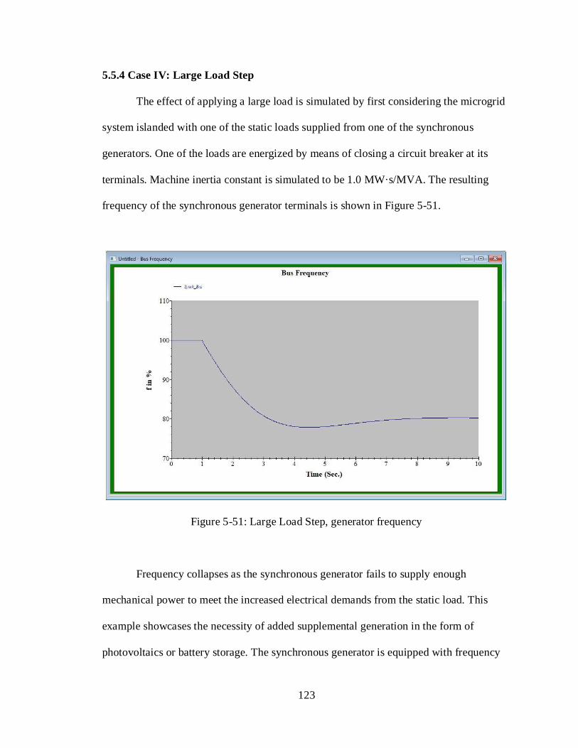
123
5.5.4 Case IV: Large Load Step
The effect of applying a large load is simulated by first considering the microgrid
system islanded with one of the static loads supplied from one of the synchronous
generators. One of the loads are energized by means of closing a circuit breaker at its
terminals. Machine inertia constant is simulated to be 1.0 MW·s/MVA. The resulting
frequency of the synchronous generator terminals is shown in Figure 5-51.
Figure 5-51: Large Load Step, generator frequency
Frequency collapses as the synchronous generator fails to supply enough
mechanical power to meet the increased electrical demands from the static load. This
example showcases the necessity of added supplemental generation in the form of
photovoltaics or battery storage. The synchronous generator is equipped with frequency

124
relays monitors the terminal frequency. One possible improvement is to enable
supplementary generation from the DC system when detecting under-frequency
conditions. The SEL700G relays for the synchronous generators have frequency
monitoring capabilities, which can be utilized to monitor the decrease in generator
terminal frequencies and send trip commands to nearby supplementary generation to turn
on. This case study does not consider grid-connected mode, as the utility will be able to
supply the necessary demands.
5.5.5 Transient Stability Summary
Several case studies were conducted on the transient stability section to analyze
and investigate possible transient stability improvement methods. The application of the
swing equation was investigated in Case I with deviations of machine’s rotor angle with
respect to faults. The biggest issue encountered in transient stability studies was the
uncertainty in exact system inertia in the form of rotating machinery. As synchronous
machineries utilized in the microgrid have inherently low machine inertia as well as low
time constants associated with asymmetrical short circuit current, it is difficult to model
machines in ETAP precisely. ETAP can plot mechanical and electrical power outputs on
the scale of MW and MW mechanical—however, generators are rated at 250W.
Additionally, several case studies did not investigate the effect of motor dynamics, in that
the induction motor was assumed to be de-energized throughout our study. Future work
may characterize and explore the effect of loading the induction motor. However, the
microgrid cannot sustain ramping the induction motor with the synchronous generator
alone, and will need to be supplemented with alternative sources of generation. Case III

125
investigated the possibility of implementing control schemes such as governor or
excitation control to improve transient stability in the microgrid. It will be important to
consider the very low time constants associated with machine currents and low rotational
inertia in implementing such a design. Lastly, there are several relay elements available
in the microgrid that closely monitor parameters such as frequencies and over/under
voltage conditions. These can be utilized to help turn on/off elements including
supplementary generation such as that from the DC subsystem.

126
Chapter 6: Conclusion
Advancements in renewable energy technologies along with their decreasing costs
and renewable energy mandates are shifting the power industry away from the centralized
generation model and instead incorporate distributed energy resources close to end users
to meet the electrical demands of the customer. The modern microgrid has capabilities of
operating in both islanded and grid-connected modes to help supplement the transfer of
energy. This thesis aims to develop the foundation of an ETAP model of the system and
test its performance of the current development iteration of the Cal Poly microgrid lab.
Several case studies and system validations comparing the ETAP model with the Cal
Poly microgrid were conducted in Chapter 5, showcasing the powerful analysis tools
ETAP can offer. Successful replication of both short circuit and protection coordination
studies were validated for both the hardware and ETAP implementations of the
microgrid. Specifically, identical relay protection settings were implemented in both SEL
microprocessor based relays as well as its equivalent model in ETAP. Additionally, the
appendix includes an ETAP protection tutorial created to aid future power system
students. This thesis therefore may serve to help supplement reference [4] and assist in
the preparation of students entering the power industry.
6.1 Difficulties Encountered
Load flow and transient stability studies were the most difficult studies to
accurately model the Cal Poly microgrid due to several considerations: non-ideal low
rated equipment, low time constants associated with dampening of transients, and low

127
system inertia, discussed throughout Chapter 5. Magnetizing current and transformer
saturation could not be modeled in ETAP load flow analysis, resulting in less current
flowing throughout the system and higher overall bus voltages. ETAP is originally
designed to model industrial scale and larger power systems, whereas the rotating
machineries in the Cal Poly’s microgrid lab are rated at one-third horse power with very
low rotational inertia. Future students must take these considerations into account if they
wish to utilize ETAP in the modeling of transient stability or other dynamic studies such
as motor acceleration.
ETAP is also incapable of modeling the entire functionality of the SEL relays
offered from SEL microprocessor based relays. Per reference [4], the prior microgrid
demonstrated SEL-311L’s permissive trip and mho distance protection, which are not
available in the Cal Poly version of ETAP 16.2. However, coordination was still
implemented primarily utilizing time overcurrent protection and demonstrated throughout
Chapter 5.
6.2 Recommended Future Work
Per reference [4], the Cal Poly San Luis Obispo’s electrical engineering
department proposed the “Advanced Power Systems Initiatives to better prepare its
students for entering the power industry.” Since ETAP is a widely used software in the
power industry, it will be beneficial for power students to learn ETAP and conduct
projects using ETAP. The Appendix includes a custom step-by-step tutorial of protection
and coordination studies conducted through ETAP. Possible future senior design projects
or master’s theses may focus on the ETAP development of SEL based laboratory

128
experiments created by the author of [4] to include simulations of the laboratory
experiments. Additionally, several functionalities of SEL relays are not currently utilized,
which can be incorporated in both the hardware and ETAP implementations of the
microgrid for future senior design and master’s theses. Overcurrent protection is not
implemented for the synchronous generator relays SEL700G. Directional protection is
available for both SEL-311L and SEL-421, but not currently implemented within the
microgrid. Frequency relays from SEL-421 can also be utilized to monitor transient
events and assert commands as necessary.
Several work may be done on the DC subsystem, which can be improved and
analyzed in more detail for the future microgrid. The addition of battery storage will
heavily relieve the energy demands of the system when operating in islanded conditions.
The two synchronous generators cannot adequately supply all the loads without
substantial decreases in generator speeds, system frequencies, and bus voltages in
islanded mode. Photovoltaics and energy storage systems will greatly relieve power
demands from the generators. Power quality analysis can be performed with the harmonic
analysis mode in ETAP to investigate the distortions of inverter current waveforms.
ETAP also has capabilities of DC short circuit analysis. DC protection and coordination
can be conducted throughout ETAP and tested with the future microgrid, similar to AC
protection implemented in this thesis.
Lastly, in the hardware implementation of the microgrid there exists no feedback
control to adjust the field current or speed of the prime mover for the synchronous
generator. Control schemes may be investigated in detail in ETAP for excitation and
governor control. However, future students will need to take into consideration the very

129
low time constants and inertia associated with the rotating machinery, which may prove
difficult to model accurately.
130
REFERENCES
[1] “The Utility View Of Microgrids,” Utility Dive. 2014.
[2] A. Majzoobi and A. Khodaei, “Application of microgrids in providing ancillary
services to the utility grid,” Energy, vol. 123, pp. 555-563, Mar. 2017.
[3] P. Denholm, M. O'Connell, G. Brinkman, and J. Jorgenson, "Overgeneration from
Solar Energy in California: A Field Guide to the Duck Chart," National
Renewable Energy Laboratory, Golden, CO, 2015.
[4] K. Pretzer, “Protective Relaying Student Laboratory,” Master’s Thesis, Dept.
Elect. Eng., California Polytechnic State Univ., San Luis Obispo, 2017.
[5] P. Kundur et al., "Definition and classification of power system stability
IEEE/CIGRE joint task force on stability terms and definitions," in IEEE
Transactions on Power Systems, vol. 19, no. 3, pp. 1387-1401, Aug. 2004.
[6] R. Majumder, "Some Aspects of Stability in Microgrids," in IEEE Transactions
on Power Systems, vol. 28, no. 3, pp. 3243-3252, Aug. 2013.
[7] R. Singh and M. Kirar, "Transient stability analysis and improvement in
microgrid," 2016 International Conference on Electrical Power and Energy
Systems (ICEPES), Bhopal, 2016, pp. 239-245.
[8] P. Kundur, N. J. Nalu, and M. G. Lauby. Power System Stability and Control.
New York: McGraw-Hill, 1994. Print.
[9] J. McCalley. EE 554. Class Lecture, Topic: “Preliminary Fundamentals.” College
of Engineering, Iowa State University, Ames, Iowa, Spring 2009.
[10] ETAP 14.1 User Guide. Operation Technology, Inc.
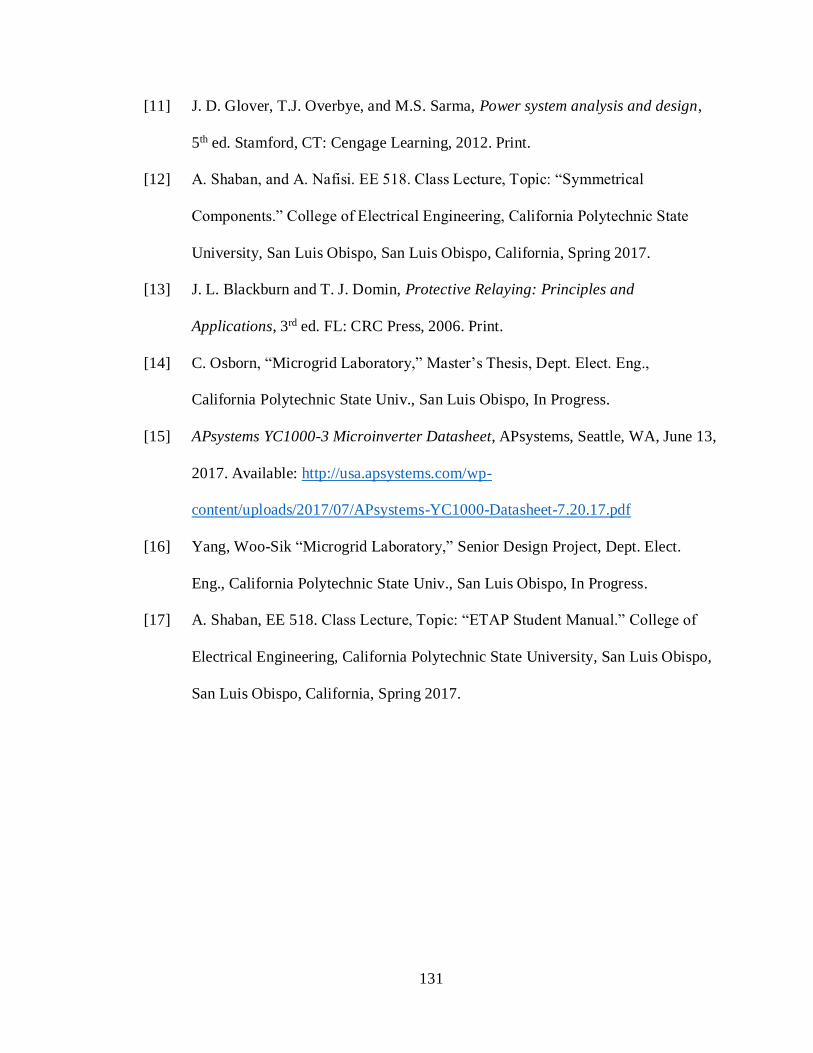
131
[11] J. D. Glover, T.J. Overbye, and M.S. Sarma, Power system analysis and design,
5th ed. Stamford, CT: Cengage Learning, 2012. Print.
[12] A. Shaban, and A. Nafisi. EE 518. Class Lecture, Topic: “Symmetrical
Components.” College of Electrical Engineering, California Polytechnic State
University, San Luis Obispo, San Luis Obispo, California, Spring 2017.
[13] J. L. Blackburn and T. J. Domin, Protective Relaying: Principles and
Applications, 3rd ed. FL: CRC Press, 2006. Print.
[14] C. Osborn, “Microgrid Laboratory,” Master’s Thesis, Dept. Elect. Eng.,
California Polytechnic State Univ., San Luis Obispo, In Progress.
[15] APsystems YC1000-3 Microinverter Datasheet, APsystems, Seattle, WA, June 13,
2017. Available: http://usa.apsystems.com/wp-
content/uploads/2017/07/APsystems-YC1000-Datasheet-7.20.17.pdf
[16] Yang, Woo-Sik “Microgrid Laboratory,” Senior Design Project, Dept. Elect.
Eng., California Polytechnic State Univ., San Luis Obispo, In Progress.
[17] A. Shaban, EE 518. Class Lecture, Topic: “ETAP Student Manual.” College of
Electrical Engineering, California Polytechnic State University, San Luis Obispo,
San Luis Obispo, California, Spring 2017.

132
APPENDICES
Appendix A: ETAP Protection Tutorial
INTRODUCTION
The following documentation has been created to assist power students
familiarize themselves with ETAP and protective relaying principles. Working through
the following example is similar to that assigned in EE 407 and EE 518. Consider Figure
A1 which illustrates a one-line of a 34.5-kV radial system per reference [1], example
10.4. The audience is intended to have gone through the example prior to its
implementation in ETAP. Select current tap settings (TSs), and time-dial settings (TDSs)
to protect the system from any fault. Assume three Westinghouse CO-8 relays for each
breaker, with a 0.3 second coordination time interval. Assume 5 cycle breaker operating
time. Assume 34.5-kV nominal line-to-line voltages at each bus for nominal operation.
Tables 1 and 2 provide necessary data in the implementation of the problem in ETAP.
Figure A2 provides a CO-8 time-delay overcurrent relay characteristics.
Figure A1: Radial System [11]

133
Table A1: Loading and Max Fault data [11]
BUS S MVA Lagging PF Max 3-phase bolted fault current (A)
1 11.0 0.95 3000
2 4.0 0.95 2000
3 6.0 0.95 1000
Table A2: Breaker Operating time and CT Ratio [11]
Breaker Breaker Operating Time CT Ratio Relay
CB1 5 cycles 400:5 CO-8
CB2 5 cycles 200:5 CO-8
CB3 5 cycles 200:5 CO-8

134
Figure A2: CO-8 time-delay overcurrent relay characteristics [11]
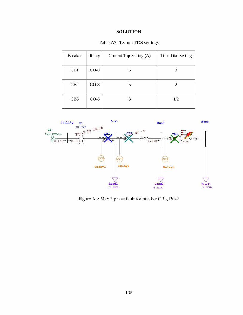
135
SOLUTION
Table A3: TS and TDS settings
Breaker Relay Current Tap Setting (A) Time Dial Setting
CB1 CO-8 5 3
CB2 CO-8 5 2
CB3 CO-8 3 1/2
Figure A3: Max 3 phase fault for breaker CB3, Bus2

136
Figure A4: Sequence-of-Operation for Figure A3
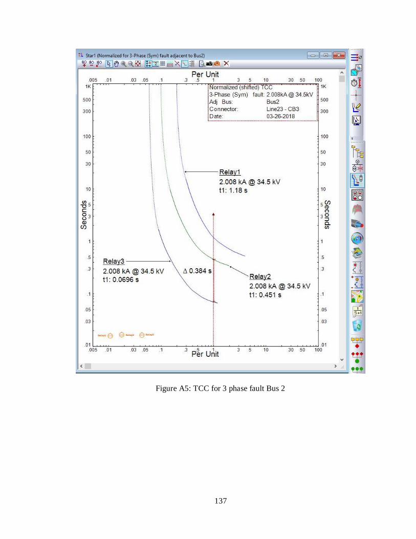
137
Figure A5: TCC for 3 phase fault Bus 2

138
Part 1: Setting up ETAP One-Line
Open ETAP 16.2.0 and create a new project from File > New Project. Enter a
name for the new project, e.g. “protection” and press OK shown in Figure A6.
Figure A6: ETAP, New Project
When prompted for user information, default values are acceptable and Access
level permissions should all be selected to provide the user with the highest level of
access and press OK. At this point, you should see an empty one-line diagram in which
we will create our radial power system.
Create four buses by left clicking an AC Bus ( ) from the AC Edit toolbar
and placing them on the empty one-line diagram. ETAP automatically labels the buses as
“Bus1”, “Bus2”, etc. Double left click any bus on the one-line diagram to open up the

139
Bus Editor which has several tabs available to the user to vary bus parameters. Select the
Info tab if not already selected, and change the Nominal kV for Bus1 to 34.5 kV and hit
OK. Repeat the process for Bus2 and Bus3. Hit Ctrl+z at anytime on the one-line
diagram to revert any misoperation.
Figure A7: ETAP, Placing AC Bus, one-line
Double left click Bus4, select Info tab and edit its name under ID to “Utility” and
change the Nominal kV to 345 kV and hit OK. Right click any bus on the one-line and
click Rotate > 90 to reorient the buses. At this point you should arrange your
components on the one-line diagram such that it resembles Figure A7. Feel free to move
around Bus labels on the one-line diagram by left click, hold, and dragging. Figure A8
shows the Bus Editor for the Utility bus.
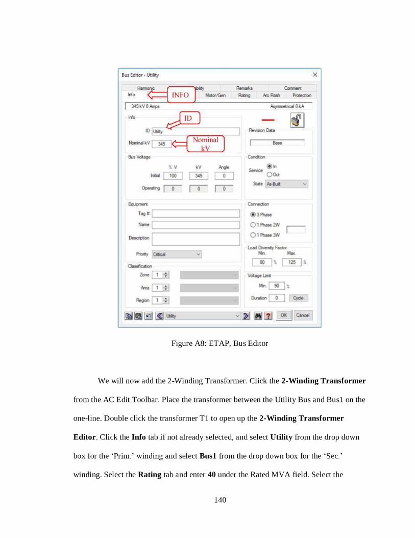
140
Figure A8: ETAP, Bus Editor
We will now add the 2-Winding Transformer. Click the 2-Winding Transformer
from the AC Edit Toolbar. Place the transformer between the Utility Bus and Bus1 on the
one-line. Double click the transformer T1 to open up the 2-Winding Transformer
Editor. Click the Info tab if not already selected, and select Utility from the drop down
box for the ‘Prim.’ winding and select Bus1 from the drop down box for the ‘Sec.’
winding. Select the Rating tab and enter 40 under the Rated MVA field. Select the

141
Impedance tab and select Typical Z & X/R. We have selected typical impedance values
for this transformer for purposes of simulation. Click OK. You may need to right click
the transformer on the one-line, and select Rotate > -90 for convenient placing. Figure
A9 displays the entering of transformer parameters and its placement on the one-line.
Figure A9: ETAP, Transformer Editor, one-line
We will now add the Power Grid. Click the Power Grid from AC Edit Toolbar.
Place the power grid to the left of the Utility Bus on the one-line. Double click the power
grid U1 to open up the Power Grid Editor. Click the Info tab if not already selected, and
select Utility from the drop down box for the Bus. Select the Short Circuit tab and enter
500 under the MVAsc 3-Phase SC Rating field. Enter 10 under the X/R field. We have
selected typical short circuit contributions from the power grid for purposes of
simulation. Click OK. Figure A10 displays the entering of power grid parameters and its
placement on the one-line.

142
Figure A10: ETAP, Power Grid Editor, one-line
We will now add two transmission lines. The complete realization of a
transmission line requires several considerations to model. The interested reader may
refer to reference [2] for a more detailed understanding of transmission line
parameterization. Click the Transmission Line from the AC Edit Toolbar. Place the
transmission line between Bus1 and Bus2. Double click the transmission line to open up
the Transmission Line Editor. Click the Info tab if not already selected, enter Line12
under ID. Select Bus1 from the drop down box ‘From’. Select Bus2 from the drop down
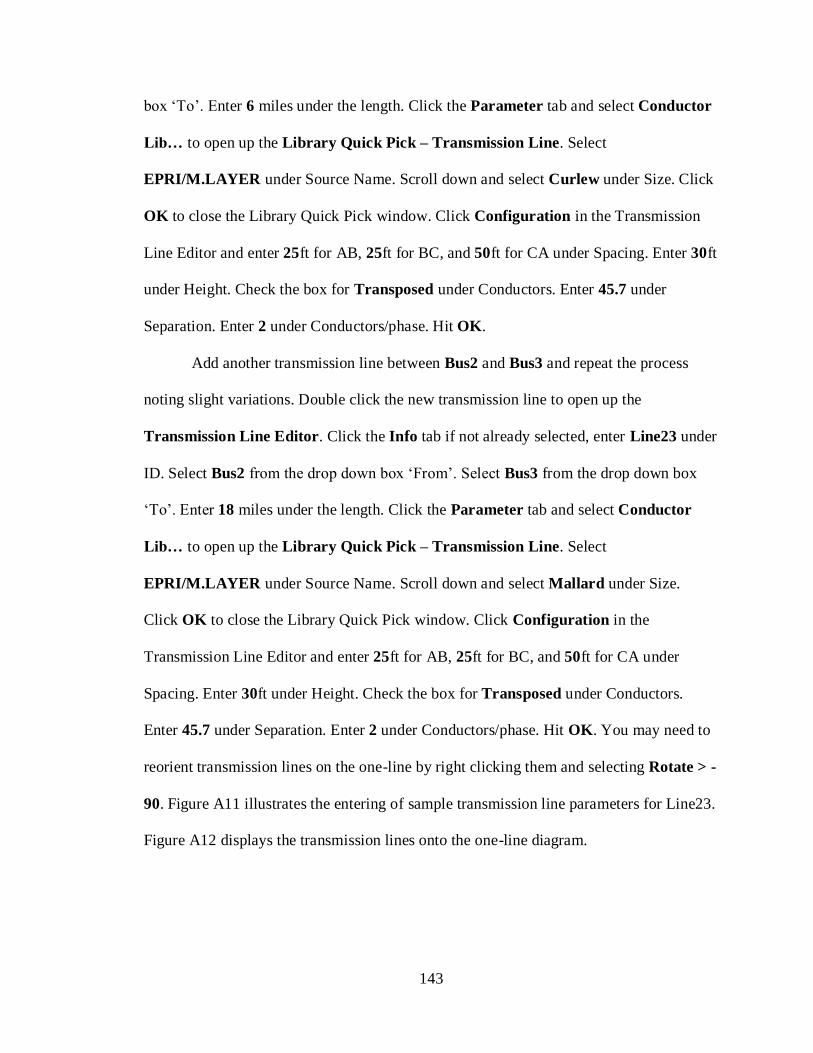
143
box ‘To’. Enter 6 miles under the length. Click the Parameter tab and select Conductor
Lib… to open up the Library Quick Pick – Transmission Line. Select
EPRI/M.LAYER under Source Name. Scroll down and select Curlew under Size. Click
OK to close the Library Quick Pick window. Click Configuration in the Transmission
Line Editor and enter 25ft for AB, 25ft for BC, and 50ft for CA under Spacing. Enter 30ft
under Height. Check the box for Transposed under Conductors. Enter 45.7 under
Separation. Enter 2 under Conductors/phase. Hit OK.
Add another transmission line between Bus2 and Bus3 and repeat the process
noting slight variations. Double click the new transmission line to open up the
Transmission Line Editor. Click the Info tab if not already selected, enter Line23 under
ID. Select Bus2 from the drop down box ‘From’. Select Bus3 from the drop down box
‘To’. Enter 18 miles under the length. Click the Parameter tab and select Conductor
Lib… to open up the Library Quick Pick – Transmission Line. Select
EPRI/M.LAYER under Source Name. Scroll down and select Mallard under Size.
Click OK to close the Library Quick Pick window. Click Configuration in the
Transmission Line Editor and enter 25ft for AB, 25ft for BC, and 50ft for CA under
Spacing. Enter 30ft under Height. Check the box for Transposed under Conductors.
Enter 45.7 under Separation. Enter 2 under Conductors/phase. Hit OK. You may need to
reorient transmission lines on the one-line by right clicking them and selecting Rotate > -
90. Figure A11 illustrates the entering of sample transmission line parameters for Line23.
Figure A12 displays the transmission lines onto the one-line diagram.

144
Figure A11: ETAP, Transmission Line Editor

145
Figure A12: ETAP, Transmission Lines, one-line
We will now add static loads to our one-line. Click the Static Load from the AC
Edit Toolbar. Place three static loads, Load1, Load2, and Load3 below Bus1, Bus2, and
Bus3, respectively. Double click Load1 from the one-line and click the Info tab if not
already selected and select Bus1 from the drop down box ‘Bus’. Click the Loading tab
and enter 11 MVA and 95 % PF. Hit OK. Double click Load2 from the one-line and
click the Info tab if not already selected and select Bus2 from the drop down box ‘Bus’.
Click the Loading tab and enter 4 MVA and 95 % PF. Hit OK. Double click Load3 from
the one-line and click the Info tab if not already selected and select Bus3 from the drop
down box ‘Bus’. Click the Loading tab and enter 6 MVA and 95 % PF. Hit OK.

146
Figure A13: ETAP, Static Loads

147
Part 2: ETAP Protection and Coordination settings
We will now modify the prior one-line to add protective elements including the
current transformer, high voltage circuit breaker, and protective relay to create the figures
shown in the solutions section above. Break the connection between transformer T1 and
Bus1 on the one-line by clicking the connector between the circuit elements and pressing
Delete. Alternatively, Right Click > Cut to remove the connection. While holding Ctrl,
click transformer T1, Utility bus, and U1 power grid, and release Ctrl, ensuring the
selected elements are highlighted in red. Click and drag the highlighted elements towards
to left to allocate more empty space between T1 and Bus1 on the one-line.
We will now add the Current Transformer (CT) and High Voltage Circuit Breaker
(HVCB) to our one-line. Select Current Transformer (CT) from the Instrumentation
Toolbar and place the CT between T1 and Bus1. Select Display Options from the AC
Edit Toolbar, select the AC tab if not already selected, and check the boxes next to PT &
CT under ID and Rating, and hit OK. This will identify and display the CT names and
ratings on the one-line. Select High Voltage Circuit Breaker (HVCB) and place the
HVCB between the CT and Bus1. Rotate both the CT and HVCB so they are horizontally
aligned by Right Click > Rotate 90. Connect the left end of the CT to transformer T1 by
clicking and holding on the pink box which appears when you point over the end of the
CT element. Connect the right end of the CT to left end of HVCB CB1. Connect the right
end of CB1 with Bus1. Figure A14 illustrates the addition of a CT and CB onto the one-
line.

148
Figure A14: ETAP, CT and CB
We will now repeat the process by adding two more sets of CTs and CBs next to
Bus1 and Bus 2, respectively. Delete the segment between Bus1 and transmission line
Line12. Add a CT and HVCB between Bus1 and Line12, rotate the protective elements
as needed, and relocate other circuit elements as necessary. Delete the segment between
Bus2 and Line23. Add a CT and HVCB between Bus2 and Line23, rotate the protective
elements as needed, and relocate other circuit elements as necessary. Figure A15 displays
the one-line with all circuit transformers and circuit breakers added to the system.
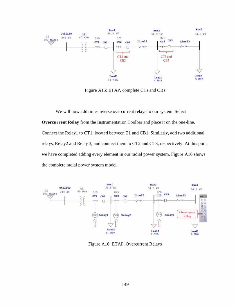
149
Figure A15: ETAP, complete CTs and CBs
We will now add time-inverse overcurrent relays to our system. Select
Overcurrent Relay from the Instrumentation Toolbar and place it on the one-line.
Connect the Relay1 to CT1, located between T1 and CB1. Similarly, add two additional
relays, Relay2 and Relay 3, and connect them to CT2 and CT3, respectively. At this point
we have completed adding every element in our radial power system. Figure A16 shows
the complete radial power system model.
Figure A16: ETAP, Overcurrent Relays
150
Part 3: Device coordination settings
We will now implement all the necessary settings to coordinate our protective
relays and circuit breakers to protect the radial system in Figure A16 from three-phase
faults. Let us first set our current transformer ratios. Double click CT1 on the one-line to
open the Current Transformer (CT) Editor and select the Rating page. Enter 400 A for
Primary under Ratio, and 5 A Secondary, leave all other settings as default values, and hit
OK. We are neglecting the effect of CT saturation for the purposes of simulation and
hence not entering CT burden values. Similarly, double click CT2 on the one-line and
select the Rating page. Enter 200 A for Primary under Ratio, 5 A Secondary, and hit OK.
Double click CT3 on the one-line and select the Rating page. Enter 200 A for Primary
under Ratio, 5 A Secondary, and hit OK. We have now successfully assigned proper CT
ratios to step down fault currents to nominal values to be fed to our relays. Figure A17
displays an example of setting CT primary and secondary settings for CT2.

151
Figure A17: ETAP, Current Transformer settings
We will now verify circuit breaker parameters for purposes of coordination.
Double click CB1 on the one-line and select the Rating page. Select 5 under the drop
down ‘Cycle.’ Leave all other parameters as default and hit OK. We have successfully
ensured a 5 cycle (83.3 ms) operating time for the circuit breaker. ETAP has an extensive
library of circuit breakers, but we are concerned primarily with the rated interrupting time
for purposes of simulation. Repeat the process above for CB2 and CB3. Figure A18
displays an example of setting circuit breaker settings for CB1.
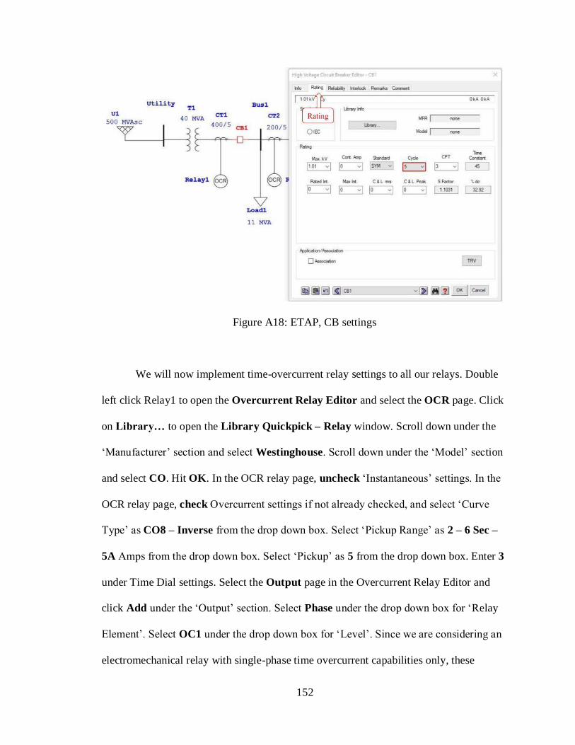
152
Figure A18: ETAP, CB settings
We will now implement time-overcurrent relay settings to all our relays. Double
left click Relay1 to open the Overcurrent Relay Editor and select the OCR page. Click
on Library… to open the Library Quickpick – Relay window. Scroll down under the
‘Manufacturer’ section and select Westinghouse. Scroll down under the ‘Model’ section
and select CO. Hit OK. In the OCR relay page, uncheck ‘Instantaneous’ settings. In the
OCR relay page, check Overcurrent settings if not already checked, and select ‘Curve
Type’ as CO8 – Inverse from the drop down box. Select ‘Pickup Range’ as 2 – 6 Sec –
5A Amps from the drop down box. Select ‘Pickup’ as 5 from the drop down box. Enter 3
under Time Dial settings. Select the Output page in the Overcurrent Relay Editor and
click Add under the ‘Output’ section. Select Phase under the drop down box for ‘Relay
Element’. Select OC1 under the drop down box for ‘Level’. Since we are considering an
electromechanical relay with single-phase time overcurrent capabilities only, these

153
settings will be limited. For more sophisticated relays such as Schweitzer Engineering
Laboratories (SEL), many relay elements such as differential, negative sequence, etc.
would be available. Click Add under the Interlock section. Select ‘Device Type’ as
HVCB, ‘Device ID’ as CB1, and ‘Action’ as Open under the respective drop down
boxes. Hit OK. Congratulations, we have successfully programmed current tap and time
dial settings for Relay1, and enabled the assertion of trip commands to CB1 in the event
of a fault.

154
Figure A19: ETAP, Relay OCR settings

155
Figure A20: ETAP, Relay Output settings
We will now repeat the process for Relay2 and Relay3 for their respective relay
settings for a Westinghouse CO8 electromechanical relay. Double left click Relay2 to
open the Overcurrent Relay Editor and select the OCR page. Click on Library… to
open the Library Quickpick – Relay window. Scroll down under the ‘Manufacturer’
section and select Westinghouse. Scroll down under the ‘Model’ section and select CO.
Hit OK. In the OCR relay page, uncheck ‘Instantaneous’ settings. In the OCR relay
page, check Overcurrent settings if not already checked, and select ‘Curve Type’ as CO8
– Inverse from the drop down box. Select ‘Pickup Range’ as 2 – 6 Sec – 5A Amps from

156
the drop down box. Select ‘Pickup’ as 5 from the drop down box. Enter 2 under Time
Dial settings. Select the Output page in the Overcurrent Relay Editor and click Add
under the ‘Output’ section. Select Phase under the drop down box for ‘Relay Element’.
Select OC1 under the drop down box for ‘Level’. Click Add under the Interlock section.
Select ‘Device Type’ as HVCB, ‘Device ID’ as CB2, and ‘Action’ as Open under the
respective drop down boxes. Hit OK.
Double left click Relay3 to open the Overcurrent Relay Editor and select the
OCR page. Click on Library… to open the Library Quickpick – Relay window. Scroll
down under the ‘Manufacturer’ section and select Westinghouse. Scroll down under the
‘Model’ section and select CO. Hit OK. In the OCR relay page, uncheck ‘Instantaneous’
settings. In the OCR relay page, check Overcurrent settings if not already checked, and
select ‘Curve Type’ as CO8 – Inverse from the drop down box. Select ‘Pickup Range’ as
2 – 6 Sec – 5A Amps from the drop down box. Select ‘Pickup’ as 3 from the drop down
box. Enter 0.5 under Time Dial settings. Select the Output page in the Overcurrent Relay
Editor and click Add under the ‘Output’ section. Select Phase under the drop down box
for ‘Relay Element’. Select OC1 under the drop down box for ‘Level’. Click Add under
the Interlock section. Select ‘Device Type’ as HVCB, ‘Device ID’ as CB3, and ‘Action’
as Open under the respective drop down boxes. Hit OK.

157
Part 3: ETAP Protection Analysis
For the purposes of this custom tutorial, we will generate time-current
characteristics (TCC) for the radial power system protection scheme. For the interested
reader, ETAP provides a tutorial for its protection analysis capabilities (STAR) by
clicking Help > Help Search on the ETAP menu-bar which opens the ETAP Help
16.1.0 window. Select Tutorials > Star Tutorial for extensive background for all STAR
basics.
Up until this point we have been operating under the ‘Edit’ mode to create our
radial power system and change power system parameters as needed. We will now switch
the ETAP presentation from ‘Edit’ mode to Star – Protection & Coordination mode by
clicking the icon on the Mode toolbar. Figure A21 illustrates the switching from edit
mode to Star mode in ETAP.
Figure A21: ETAP, Star mode
ETAP allows us to modify the Star Mode study case to adjust parameters such as
fault type (3 phase, line-to-line, etc.), fault value (symmetrical/asymmetrical), fault

158
impedance, etc. for in depth analysis. For purposes of this tutorial we will consider
default ETAP Star parameters e.g. three-phase faulted conditions. Click on Fault
Insertion from the STAR toolbar and apply the fault by left clicking the segment to the
right of CB3 at Bus2, which is the largest fault current Relay3 will detect (2 kA). If
prompted for an ‘Output File Name’, enter ‘3phase’ or any other name of your choosing.
If coordinated correctly, you should observe three circuit breakers marked with an ‘X’
next to a number indicating the order of circuit breaker tripping operation, illustrated in
Figure A22.
Figure A22: ETAP, three-phase fault, Bus2
For a more analytical description showcasing the sequence of operation of
protective elements shown in Figure A22, click Sequence Viewer from the STAR
toolbar which opens the Sequence-of-Operation (SQOP) Events window shown in Figure
A23. SQOP allows us to systematically confirm if our protective relaying settings and
circuit breaker operation adhere to design considerations outlined in the problem

159
statement. The Time (ms) column in Figure A22 indicates the time in which certain
protective elements have asserted commands. T1 (ms) indicates the operating time of
protective elements. For example, at time 69.5 ms, Relay3 has asserted trip commands to
open CB3, and at time 153 ms the fault has been cleared by CB3 (5 cycle clearing time,
83.3 ms). To provide backup protection, Relay2 asserts trip commands at time 450 ms,
following by the clearing of the fault of CB2. Finally, Relay1 and CB1 provides a third
layer of protection.
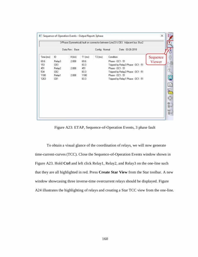
160
Figure A23: ETAP, Sequence-of-Operation Events, 3 phase fault
To obtain a visual glance of the coordination of relays, we will now generate
time-current-curves (TCC). Close the Sequence-of-Operation Events window shown in
Figure A23. Hold Ctrl and left click Relay1, Relay2, and Relay3 on the one-line such
that they are all highlighted in red. Press Create Star View from the Star toolbar. A new
window showcasing three inverse-time overcurrent relays should be displayed. Figure
A24 illustrates the highlighting of relays and creating a Star TCC view from the one-line.
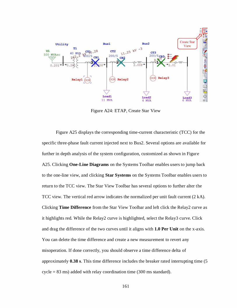
161
Figure A24: ETAP, Create Star View
Figure A25 displays the corresponding time-current characteristic (TCC) for the
specific three-phase fault current injected next to Bus2. Several options are available for
further in depth analysis of the system configuration, customized as shown in Figure
A25. Clicking One-Line Diagrams on the Systems Toolbar enables users to jump back
to the one-line view, and clicking Star Systems on the Systems Toolbar enables users to
return to the TCC view. The Star View Toolbar has several options to further alter the
TCC view. The vertical red arrow indicates the normalized per unit fault current (2 kA).
Clicking Time Difference from the Star View Toolbar and left click the Relay2 curve as
it highlights red. While the Relay2 curve is highlighted, select the Relay3 curve. Click
and drag the difference of the two curves until it aligns with 1.0 Per Unit on the x-axis.
You can delete the time difference and create a new measurement to revert any
misoperation. If done correctly, you should observe a time difference delta of
approximately 0.38 s. This time difference includes the breaker rated interrupting time (5
cycle = 83 ms) added with relay coordination time (300 ms standard).
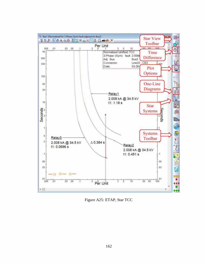
162
Figure A25: ETAP, Star TCC

163
Appendix B: SEL-421 Relay Settings
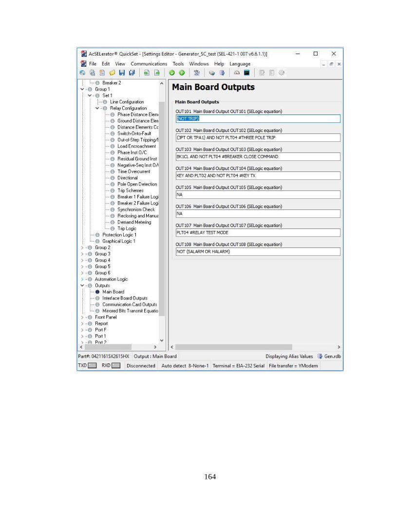
164

165
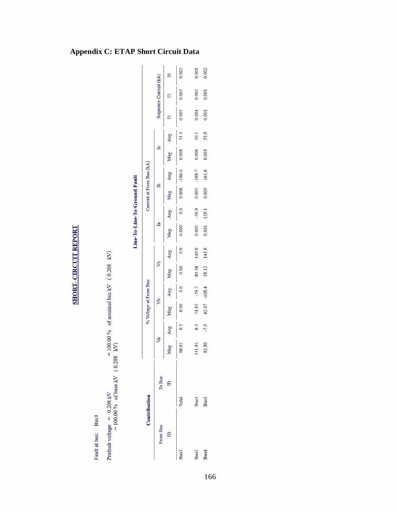
166
Appendix C: ETAP Short Circuit Data

167
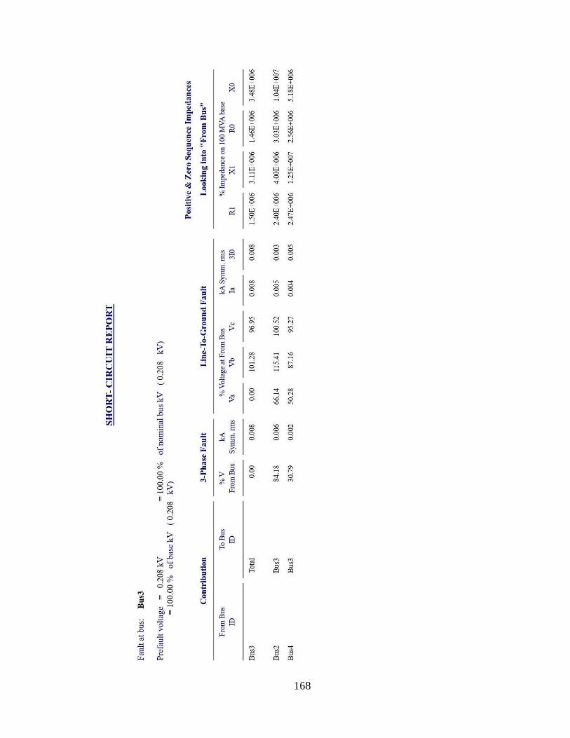
168

169
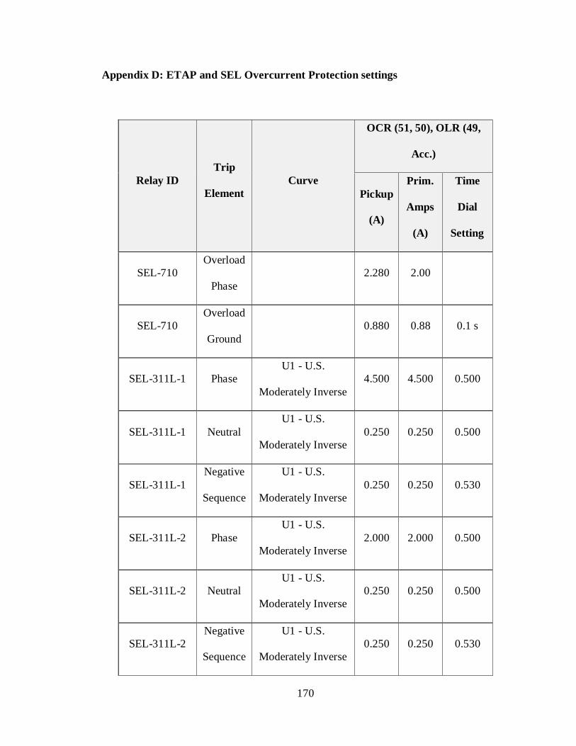
170
Appendix D: ETAP and SEL Overcurrent Protection settings
Relay ID
Trip
Element
Curve
OCR (51, 50), OLR (49,
Acc.)
Pickup
(A)
Prim.
Amps
(A)
Time
Dial
Setting
SEL-710
Overload
Phase
2.280 2.00
SEL-710
Overload
Ground
0.880 0.88 0.1 s
SEL-311L-1 Phase
U1 - U.S.
Moderately Inverse
4.500 4.500 0.500
SEL-311L-1 Neutral
U1 - U.S.
Moderately Inverse
0.250 0.250 0.500
SEL-311L-1
Negative
Sequence
U1 - U.S.
Moderately Inverse
0.250 0.250 0.530
SEL-311L-2 Phase
U1 - U.S.
Moderately Inverse
2.000 2.000 0.500
SEL-311L-2 Neutral
U1 - U.S.
Moderately Inverse
0.250 0.250 0.500
SEL-311L-2
Negative
Sequence
U1 - U.S.
Moderately Inverse
0.250 0.250 0.530

171
Relay ID
Trip
Element
Curve
OCR (51, 50), OLR (49,
Acc.)
Pickup
(A)
Prim.
Amps
(A)
Time
Dial
Setting
SEL-587 Phase
U1 - U.S.
Moderately Inverse
2.000 2.000 0.600
SEL-587
Negative
Sequence
U1 - U.S.
Moderately Inverse
0.500 0.500 0.600
SEL-387E Phase
U1- U.S.
Moderately Inverse
4.500 4.500 0.600
SEL-387E
Negative
Sequence
U1- U.S.
Moderately Inverse
0.500 0.500 0.600