Modeling, Analysis & Control of Dynamic...

MechatronicsPhysical Modeling - General

K. Craig1

P h y s ic a lS y s t e m

P h y s ic a lM o d e l

M a t hM o d e l

M o d e lP a r a m e t e r

I D

A c t u a lD y n a m icB e h a v io r

C o m p a r eP r e d ic t e dD y n a m icB e h a v io r

M a k eD e s ig n

D e c is io n s

D e s ig nC om p le t e

Measurements,Calculations,

Manufacturer's Specifications

Assumptionsand

Engineering Judgement

Physical LawsExperimentalAnalysis

Equation Solution:Analytical

and NumericalSolution

Model Adequate,Performance Adequate

Model Adequate,Performance Inadequate

Modify or

Augment

Model Inadequate:Modify

D y n a m ic S y s t e m I n v e s t ig a t io n

Which Parameters to Identify?What Tests to Perform?


K. Craig2

Physical Modeling:From Physical System to Physical Model

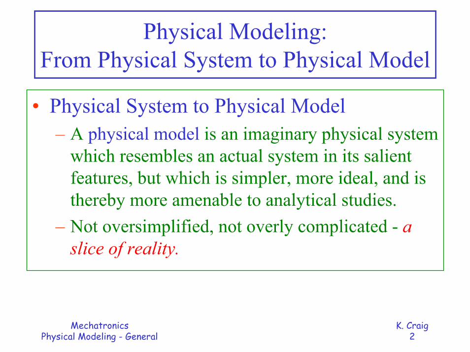
• Physical System to Physical Model– A physical model is an imaginary physical system

which resembles an actual system in its salient features, but which is simpler, more ideal, and is thereby more amenable to analytical studies.

– Not oversimplified, not overly complicated - a slice of reality.


K. Craig3

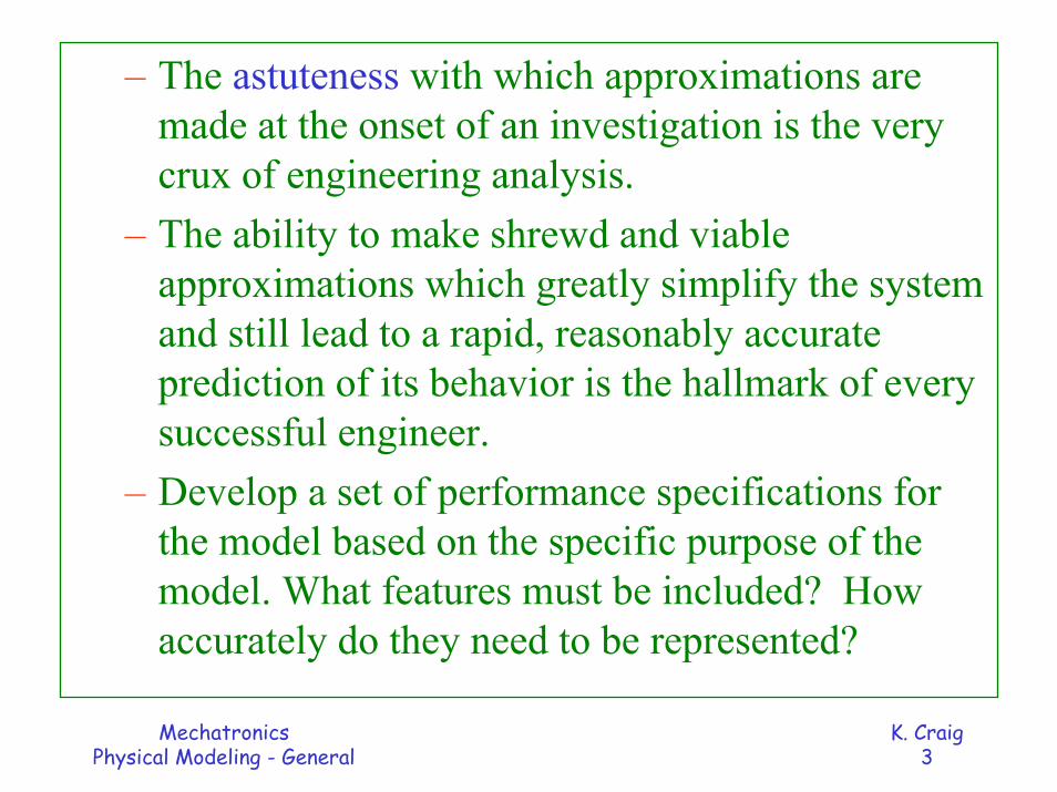
– The astuteness with which approximations are made at the onset of an investigation is the very crux of engineering analysis.

– The ability to make shrewd and viable approximations which greatly simplify the system and still lead to a rapid, reasonably accurate prediction of its behavior is the hallmark of every successful engineer.

– Develop a set of performance specifications for the model based on the specific purpose of the model. What features must be included? How accurately do they need to be represented?


K. Craig4

– The challenges to physical modeling are formidable:• Dynamic behavior of many physical processes

is complex.• Cause and effect relationships are not easily

discernible.• Many important variables are not readily

identified.• Interactions among the variables are hard to

capture.

– Engineering Judgment is the Key!


K. Craig5

– In modeling dynamic systems, we use engineering judgment and simplifying assumptions to develop a physical model.

– The complexity of the physical model depends on the particular need, e.g., system design iteration, control system design, control design verification, physical understanding.

– The intelligent use of simple physical models requires that we have some understanding of what we are missing when we choose the simpler model over the more complex model.


K. Craig6

– In modeling dynamic systems, we consider matter and energy as being continuously, though not necessarily uniformly, distributed over the space within the system boundaries.

– This is the macroscopic or continuum point of view. We consider the system variables as quantities which change continuously from point to point in the system as well as with time and this always leads to a distributed-parameter physical model which results in a partial differential equation mathematical model.


K. Craig7

– Models in this most general form behave most like the real systems at the macroscopic level.

– Because of the mathematical complexity of these models, engineers find it necessary and desirable to work with less exact models in many cases.

– Simpler models which concentrate matter and energy into discrete lumps are called lumped-parameter physical models and lead to ordinary differential equation mathematical models.


K. Craig8

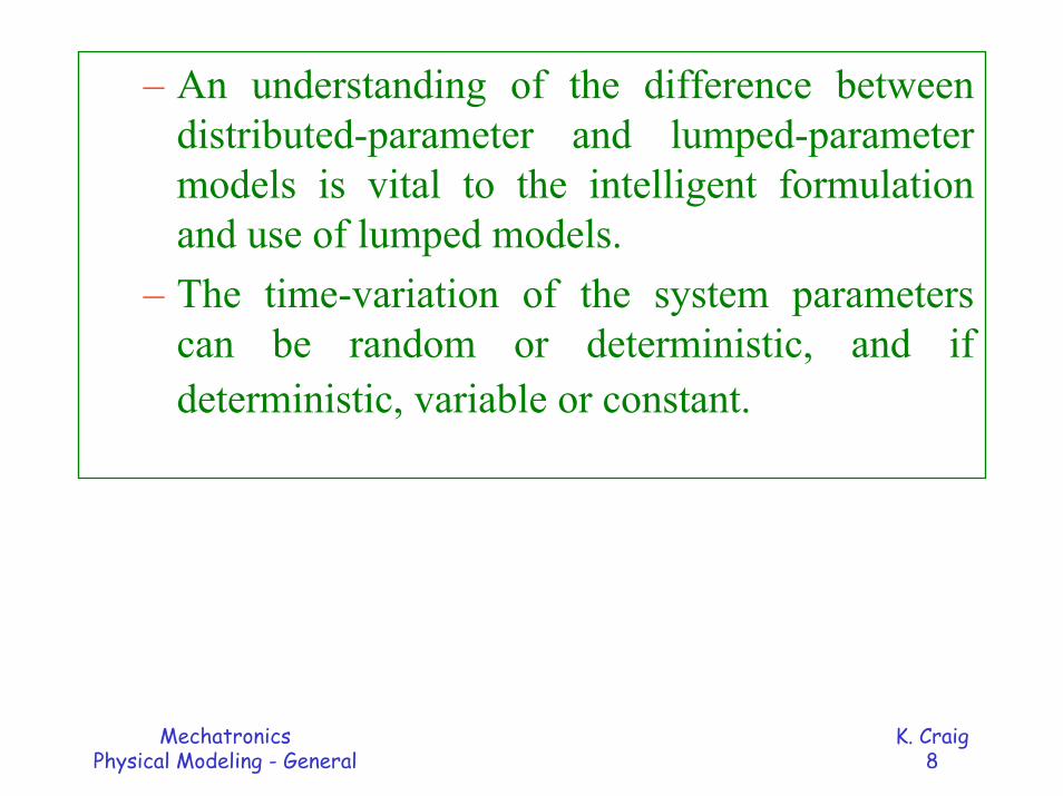
– An understanding of the difference between distributed-parameter and lumped-parameter models is vital to the intelligent formulation and use of lumped models.

– The time-variation of the system parameters can be random or deterministic, and if deterministic, variable or constant.


K. Craig9

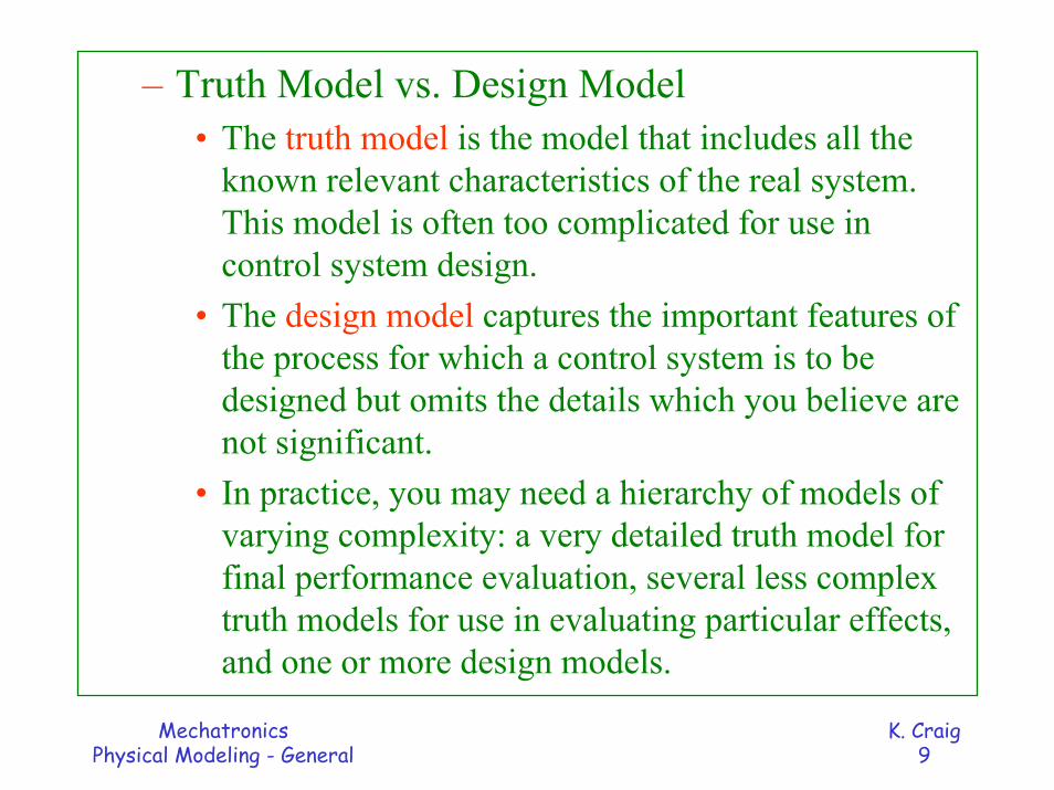
– Truth Model vs. Design Model• The truth model is the model that includes all the

known relevant characteristics of the real system. This model is often too complicated for use in control system design.

• The design model captures the important features of the process for which a control system is to be designed but omits the details which you believe are not significant.

• In practice, you may need a hierarchy of models of varying complexity: a very detailed truth model for final performance evaluation, several less complex truth models for use in evaluating particular effects, and one or more design models.


K. Craig10

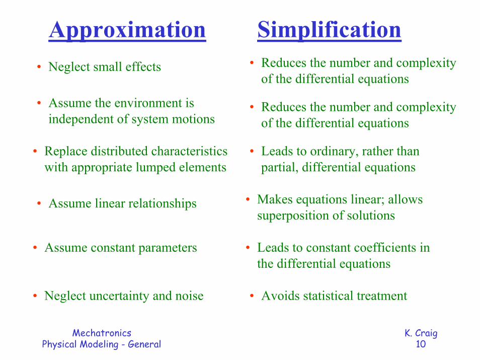
Approximation Simplification• Reduces the number and complexity

of the differential equations• Neglect small effects

• Assume the environment is independent of system motions

• Reduces the number and complexity of the differential equations

• Replace distributed characteristics with appropriate lumped elements

• Leads to ordinary, rather than partial, differential equations

• Makes equations linear; allows superposition of solutions

• Assume linear relationships

• Assume constant parameters • Leads to constant coefficients in the differential equations

• Neglect uncertainty and noise • Avoids statistical treatment


K. Craig11

• Neglect Small Effects– Small effects are neglected on a relative basis. In

analyzing the motion of an airplane, we are unlikely to consider the effects of solar pressure, the earth's magnetic field, or gravity gradient. To ignore these effects in a space vehicle problem would lead to grossly incorrect results!

• Independent Environment– In analyzing the vibration of an instrument panel in a

vehicle, we assume that the vehicle motion is independent of the motion of the instrument panel.


K. Craig12

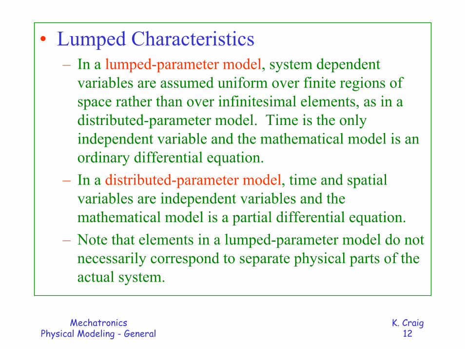
• Lumped Characteristics– In a lumped-parameter model, system dependent

variables are assumed uniform over finite regions of space rather than over infinitesimal elements, as in a distributed-parameter model. Time is the only independent variable and the mathematical model is an ordinary differential equation.

– In a distributed-parameter model, time and spatial variables are independent variables and the mathematical model is a partial differential equation.

– Note that elements in a lumped-parameter model do not necessarily correspond to separate physical parts of the actual system.


K. Craig13

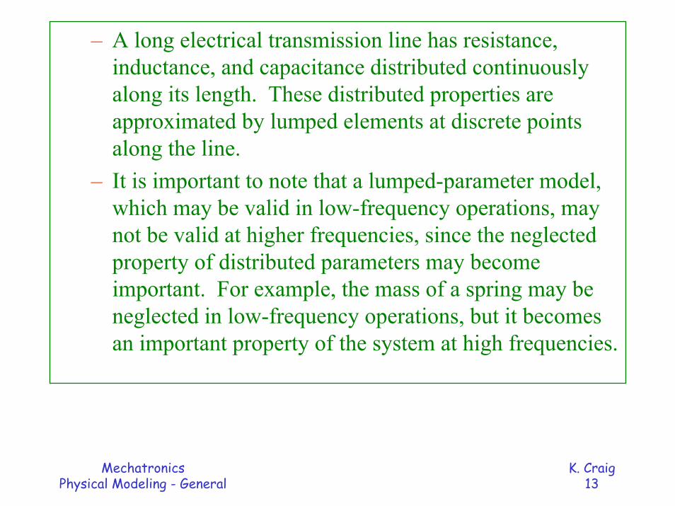
– A long electrical transmission line has resistance, inductance, and capacitance distributed continuously along its length. These distributed properties are approximated by lumped elements at discrete points along the line.

– It is important to note that a lumped-parameter model, which may be valid in low-frequency operations, may not be valid at higher frequencies, since the neglected property of distributed parameters may become important. For example, the mass of a spring may be neglected in low-frequency operations, but it becomes an important property of the system at high frequencies.


K. Craig14

• Linear Relationships– Nearly all physical elements or systems are inherently

nonlinear if there are no restrictions at all placed on the allowable values of the inputs, e.g., saturation, dead-zone, square-law nonlinearities.

– If the values of the inputs are confined to a sufficiently small range, the original nonlinear model of the system may often be replaced by a linear model whose response closely approximates that of the nonlinear model.

– When a linear equation has been solved once, the solution is general, holding for all magnitudes of motion.


K. Craig15

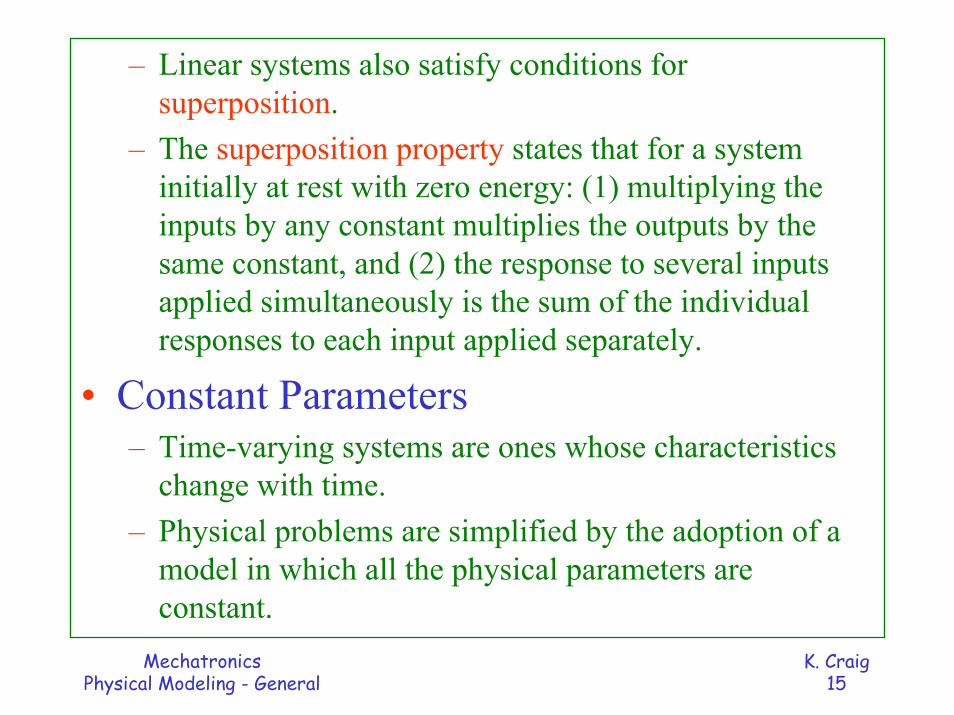
– Linear systems also satisfy conditions for superposition.

– The superposition property states that for a system initially at rest with zero energy: (1) multiplying the inputs by any constant multiplies the outputs by the same constant, and (2) the response to several inputs applied simultaneously is the sum of the individual responses to each input applied separately.

• Constant Parameters– Time-varying systems are ones whose characteristics

change with time. – Physical problems are simplified by the adoption of a

model in which all the physical parameters are constant.


K. Craig16

• Neglect Uncertainty and Noise– In real systems we are uncertain, in varying degrees,

about values of parameters, about measurements, and about expected inputs and disturbances. Disturbances contain random inputs, called noise, which can influence system behavior.

– It is common to neglect such uncertainties and noise and proceed as if all quantities have definite values that are known precisely.


K. Craig17

Classes ofSystems

LumpedParameter

DistributedParameter

DeterministicStochastic

ContinuousTime

DiscreteTime

LinearNonlinear

ConstantCoefficient

TimeVarying

HomogeneousNon-Homogeneous

Classes of Systems


K. Craig18

The most realistic physical model of a dynamic system leads to differential equations of motion that are:

nonlinear, partial differential equationswith time-varying and space-varying parameters

These equations are the most difficult to solve.

The simplifying assumptions discussed lead to a physical model of a dynamic system that is less realistic and to equations of

motion that are:

linear, ordinary differential equationswith constant coefficients

These equations are easier to solve and design with.


K. Craig19

Physical Modeling Example:44.5N Electrodynamic Vibration Shaker

Full-scale force capabilities for different models range from about 20 to 150,000 N, with permanent magnet fields being used below about 250 N.


K. Craig20

• This "moving coil" type of device converts an electrical command signal into a mechanical force and/or motion and is very common, e.g., vibration shakers, loudspeakers, linear motors for positioning heads on computer disk memories, high-speed galvanometers for oscillographic recorders and optical mirror scanners.

• In all these cases, a current-carrying coil is located in a steady magnetic field provided by permanent magnets in small devices and electrically-excited wound coils in large ones.


K. Craig21

• Two electromechanical effects are observed in such configurations: – Generator Effect:

– Motion of the coil through the magnetic field causes a voltage proportional to velocity to be induced into the coil.

– Motor Effect:– Passage of current through the coil causes it to experience

a magnetic force proportional to the current.


K. Craig22

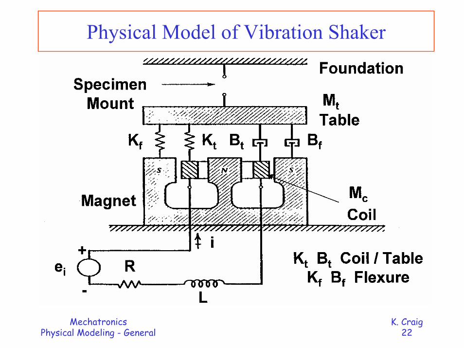
Physical Model of Vibration Shaker


K. Craig23

• Flexure Kf is an intentional soft spring (stiff, however, in the radial direction) that serves to guide the axial motion of the coil and table.

• Flexure damping Bf is usually intentional, fairly strong, and obtained by laminated construction of the flexure spring, using layers of metal, elastomer, plastic, and so on.

• The coupling of the coil to the shaker table would ideally be rigid so that magnetic force is transmitted undistorted to the mechanical load. Thus Kt (generally large) and Bt(quite small) represent parasitic effects rather than intentional spring and damper elements.

• R and L are the total circuit resistance and inductance, including contributions from both the shaker coil and the amplifier output circuit.

Modeling, Analysis & Control of Dynamic...

Documents

Transcript of Modeling, Analysis & Control of Dynamic...