Delft University of Technology

Delft Center for Systems and Control

Technical report 12-004

Modeling, analysis, and simulation of a

cryogenic distillation process for 13C

isotope separation∗

D.C. Dumitrache, B. De Schutter, A. Huesman, and E. Dulf

If you want to cite this report, please use the following reference instead:

D.C. Dumitrache, B. De Schutter, A. Huesman, and E. Dulf, “Modeling, analysis, and

simulation of a cryogenic distillation process for 13C isotope separation,” Journal of

Process Control, vol. 22, no. 4, pp. 798–808, Apr. 2012.

Delft Center for Systems and Control

Delft University of Technology

Mekelweg 2, 2628 CD Delft

The Netherlands

phone: +31-15-278.51.19 (secretary)

fax: +31-15-278.66.79

URL: http://www.dcsc.tudelft.nl

∗This report can also be downloaded via http://pub.deschutter.info/abs/12_004.html

Modeling, Analysis, and Simulation of a Cryogenic

Distillation Process for 13C Isotope Separation

Dan Calin Dumitrachea,b,∗, Bart De Schuttera, Adrie Huesmana, Eva Dulfb

aDelft Center for Systems and Control, Delft University of Technology, Mekelweg 2, 2628 CD Delft,

The NetherlandsbDepartment of Automatic Control, Technical University of Cluj-Napoca, G. Baritiu 26-28, 400027,

Cluj-Napoca, Romania

Abstract

This paper presents a structured and insightful approach to modeling and simulation of an isotopicenrichment plant that uses distillation principles for 13C isotope separation. First, after a briefreview of distillation and mass transfer-related topics, a full nonlinear model for the cryogenicdistillation process for 13C isotope separation is derived from first-principles knowledge. In orderto derive the mathematical description of the concerned isotope separation process, based on thetwo-film theory, we will derive the rate of transfer of the 13C isotope from the vapor phase to theliquid phase. Since the isotope separation by cryogenic distillation is usually carried out in a verylong column with a small diameter, a good approximation arises by neglecting the radial diffusion.We continue with the determination of the system of the partial differential equations that governsthe evolution of desired isotope during the separation process. Next, we solve the system of partialdifferential equations, resulting in the full nonlinear model. Due to the complexity of the fullnonlinear model, we consider two additional alternative modeling approaches resulting in a quasi-linear model and, when the isotope concentration achieved is low, a linear approximation model.In the second part of the paper we use the finite-differences method for the numerical analysis andnumerical simulation of the three models, followed by the assessment of the linear model for futuretasks in modeling, optimization, and process control.

Keywords:

Isotope separation, Cryogenic distillation, Modeling, Distributed parameter system, Numericalanalysis, Simulation

1. Introduction

Isotopes of various elements have different applications in a variety of fields such as hydrology,geology, and medicine [1, 2, 3]. Some of these applications have a basis in techniques like determiningthe isotopic signature of an investigated material or the use of labeled compounds for tracing themfrom one part of a system to another. These techniques provide information used in studying e.g.

∗Corresponding author. Tel.: +40 740 365 167; Fax: +40 266 313 058;E-mail address: dan.dumitrache@aut.utcluj.ro

Preprint submitted to Elsevier

Latin symbols

A area m2

c molar concentration molm3

d diameter m

D molecular diffusivity m2

s

h height m

H hold-up per unit volume molm3

HETP height equivalent to a theoretical plate m

J molar flux molm2s

K volumetric overall mass transfer coefficient molm3s

L liquid molar flow rate per unit area molm2s

M molar mass kg

mol

n 13CO mole fraction in vapor phase −

N 13CO mole fraction in liquid phase −

S separation factor −

T temperature K

V vapor molar flow rate per unit area molm2s

x liquid-phase mole fraction −

y vapor-phase mole fraction −

z height (position) m

Z total height of the column m

Greek symbols

α relative volatility −

δ film thickness m

ε enrichment factor −

θ number of trays −

κ K-value (i.e. vapor-liquid distribution ratio) −

ρ density kg

m3

σ specific interfacial area m2

m3

τ molar transfer rate per unit volume molm3s

χ mole fraction −

Ψ product flow rate molm2s

Superscript

∗ hypothetical −

0 pure component −

13 atomic number −

Subscript

0 natural abundance −

13CO isotopic species −

c column −

H is referring to H −

i index −

(I) interface −

l liquid −

L is referring to L −

τ is referring to τ −

v vapor −

V is referring to V −

Table 1: Nomenclature

2

chemical mechanisms, various biological experiments, and medical investigations. Particularly, theinterest in the 13C isotope has increased lately due to its applications in organic chemistry, oceanicand atmospheric studies, and medical diagnosis based on breath CO2 tests (13C/12C ratio), whichavoids in this way the common invasive procedures [4, 5].

The isotope separation techniques are based on the isotope effects of different isotopic com-pounds that arise from the differences in the nuclear properties of the isotopes [6]. Some practicalmethods are chemical exchange processes, diffusion-based separation, laser separation, chromatog-raphy methods, and distillation [7, 8, 9]. The isotope separation technique depends on the propertiesof the element or the chemical compound involved, the cost of the process, and on the various appli-cations that make use of different concentrations. Due to the relative large mass difference betweenthe different isotopes of light elements like boron, carbon, nitrogen, or oxygen a practical methodof isotope separation for these elements is distillation, which is based on the vapor pressure isotopeeffect [9, 10].

Urey showed in [11] that the isotopic substances differ not only in the physical and chemicalproperties related directly to mass but in their thermodynamical properties as well. Bigeleisen pro-vides in [12] a method of calculation of the equilibrium constant for the isotopic exchange reactionsthrough methods of statistical mechanics. A general and insightful review on both experimentaland theoretical work on the isotope effects with emphasis on the vapor pressure isotope effect isprovided by Jancso and Van Hook in [13]. The general theory of multistage isotope separationprocesses was developed by Cohen [14], treating issues like hold-up, enrichment, and equilibriumtime for both ideal and real cascades. The evaporative, concurrent, and countercurrent centrifugesare treated. Cohen also briefly discussed the behavior of liquid-gas countercurrent chemical ex-change towers, emphasizing that the theory is essentially the same for all of the isotope separationprocesses. London [9] also provides an insightful study on isotope separation for reversible andirreversible processes. A chapter in his work is dedicated to the isotope separation by distillationwhere he briefly presents the production of 13C by the distillation of carbon monoxide. Andreevet al. [15] treat in a descriptive way the methods used in the separation in two-phase systems ofhydrogen, carbon, nitrogen, and oxygen, providing also a review based on the characteristics ofdifferent 13C cryogenic rectification plants in a chronological order. McInteer presents in [16] designissues of a 13C cryogenic distillation plant by referring to the high-performance plant developed atLos Alamos National Laboratory in the USA. In [17] Li et al. treat the possibility of using advancedstructured packing instead of common random packing used in 13C separation from both productiv-ity and reduced consumption points of view while Dulf et al. [18] present a monitoring and controlsystem of a 13C enrichment plant. Mass transfer in fluid systems and the separation processes havebeen studied extensively, e.g. Cussler and King [19, 20] are excellent references, while in the fieldof dynamics, operation, and control of distillation columns Skogestad et al. give a comprehensiveand insightful exposition in [21, 22, 23, 24]. Regarding modeling of distributed parameter systemswe mention [25, 26, 27]. In the field of partial differential equations we acknowledge the work ofDebnath [28], while in the numerical analysis field [29, 30, 31] represent standard works.

It is well known that an insightful mathematical description of physical phenomena that occurin various systems is often a requirement for systems analysis, simulation, control design, andoptimization [27, 25]. Like most physical, chemical, or biological processes, isotope separationprocesses have a coupled time-space nature, where the input, output, and parameters can varyboth in time and space. Thus, they belong to the class of distributed parameter systems [25].

The objective of this paper is to provide a structured and comprehensive modeling approachfollowed by the simulation of a 13C isotope separation plant that makes use of the distillation of

3

carbon monoxide and hence, to provide a basis for future studies in modeling and process control.The main contributions of this study consist in the intelligible first-principles knowledge modeling ofthe 13C isotope separation process and the assessment of a full nonlinear model and two additionalapproximation models by numerical simulation. To the authors’ best knowledge we are the first totreat these issues for a 13C cryogenic distillation plant.

2. Distillation and the interphase mass transfer

Distillation processes are based on the relative volatility notion, which is a comparative measureof the vapor pressure of the components within a mixture. In most of the cases, distillation iscarried out in a tray column or in a packed column [32, 33]. Tray columns are preferred for highratios of liquid flow rate to vapor flow rate. Packed columns are a practical solution in severalsituations like low pressure drop separation, handling of corrosive chemicals, or in the case of smallcolumn diameter [20, 34]. Since the separation process considered in this paper takes place in apacked tower, packed distillation columns will be referred to in the following.

In this section we will briefly review some distillation and mass transfer-related topics relevantfor this study:

• equilibrium stage concept

• vapor-liquid equilibrium

• packed distillation columns

• mass transfer

We refer to the standard works in the field [20, 19, 22, 35] for additional information.

2.1. Equilibrium stage concept

The equilibrium stage (i.e. the theoretical tray) concept is a core concept in distillation processes.It is used for modeling and studying steady-state behavior, for both tray and packed distillationcolumns.

The equilibrium stage approach states that the vapor and the liquid streams, with the composi-tions xequil and yequil, leaving the stage are in equilibrium. At equilibrium, even if from a microscopicpoint of view, temperature, pressure, or composition continue to vary, for a macroscopic observerthere are no further changes in these variables [20, 22].

The equilibrium compositions xequil and yequil are mathematically related, as will be shown next.

2.2. Vapor-liquid equilibrium

The vapor-liquid equilibrium relates the composition of the components of a liquid mixture andits vapor at equilibrium. If the mixture is ideal, then the vapor-liquid equilibrium relationship canbe derived from Raoult’s and Dalton’s Laws, which allow the formulation of the K value (vapor-liquid distribution ratio) of a component i [20, 22]:

κi =yixi

=p0iP

(1)

where yi and xi are the vapor and the liquid mole fractions of the component i, p0i is the vaporpressure of the pure component, while P is the total pressure exerted by the gaseous mixture.

4

0 0.1 0.2 0.3 0.4 0.5 0.6 0.7 0.8 0.9 10

0.1

0.2

0.3

0.4

0.5

0.6

0.7

0.8

0.9

1

liquid mole fraction (x)

vapor

mole

fract

ion

(y)

α = 1α = 1.0069α = 1.5α = 2

0.494 0.497 0.5 0.503 0.506

0.494

0.497

0.5

0.503

0.506

liquid mole fraction (x)

vapor

mole

fract

ion

(y)

α = 1α = 1.0069

Figure 1: Vapor liquid equilibrium for a binary mixture with respect to different values of α

The relative volatility (α) between the components i and j of a mixture is defined as:

αij =κi

κj

=

yi

xi

yj

xj

=p0ip0j

(2)

where the more volatile component, by convention, is i (so in principle αij > 1).If the mixture is binary, and y and x refer to the light component, while 1− y and 1− x refer

to the heavy component, then the vapor-liquid equilibrium relationship becomes:

α =yx

1−y1−x

=

y1−y

x1−x

(3)

or, in a more common form:

y =αx

1 + (α− 1)x(4)

Figure 1 shows the nonlinear equilibrium curve for a binary mixture with respect to differentvalues of α including the relative volatility in the case of 13C the isotope separation by the distillationof carbon monoxide.

2.3. Packed distillation columns

The role of the packing in a packed distillation column is to ensure an increased contact surfacebetween the vapor and liquid phase and thus, to facilitate the mass transfer. Also the packing mustbe able to allow pressure drop for the vapor phase and at the same time an easy liquid drainage[35, 34]. For various distillation requirements different types of packing are used. In general, highfree spaces and a high surface area improve the efficiency of the packing [33].

In a packed column, the packing bed can be divided into a number of hypothetical zones that actlike equilibrium stages. These equilibrium stages are often referred to as theoretical plates [35, 20].

5

The packing height that accomplish the same separation as an equilibrium stage is referred to asthe height equivalent to a theoretical plate or HETP and it is a qualitative measure of the packingused.

If the column has θ trays (theoretical or physical), at total reflux with constant relative volatility,Fenske’s formula for the overall separation factor applies [22, 36]:

S =

(

xlgt

xhvy

)

T(

xlgt

xhvy

)

B

= αθ (5)

where xlgt and xhvy stand for the light and the heavy component liquid mole fraction while T andB stand for the top of the column respectively the bottom of the column1. Since the number oftrays is related to the height of the column (Zc) by:

θ =Zc

hHETP(6)

where hHETP is the value of the HETP, the height equivalent to a theoretical plate is determinedby:

hHETP =Zc

θ=

Zc ln(α)

ln(S)(7)

Steady-state behavior of packed columns can be modeled using a staged equilibrium model, thismodel being used in the column design, but with respect to the dynamics of a packed column, amore appropriate model is based on the mass transfer between the phases [35, 34, 22].

2.4. Interphase mass transfer

Prior to the equilibrium state, considered previously, the vapor and the liquid phase are trans-ferring mass from one to another, with a rate that can be expressed as [34]:

mass transfer rate = k × (area)× (driving force) (8)

where k is called a mass transfer coefficient and it is a diffusion rate constant that includes theeffect of diffusivity and the flow conditions, the (area) represents the effective mass transfer area,and the (driving force) is the actual cause due to which the mass transfer occurs. Since the drivingforce can be expressed in terms of concentrations, partial pressure, mole fractions, or molarity, themass transfer coefficient can also be defined in various ways [20, 19].

There are several theories for describing the mass transfer process [37, 38] among which thetwo-film theory, the penetration model, the film penetration model, the surface renewal dampededdy diffusion model, or the turbulent diffusion model. Since the two-film theory is widely used,especially for the physical insight it provides into mass transfer and its mathematically simplicity[19], we will adopt this approach.

1When the product is the heavy component, the separation is given by S =

(

xhvyxlgt

)

B(

xhvyxlgt

)

T

.

6

According to the two-film theory, at any location of the mass transfer equipment, the two-phasescompositions are assumed to be constant, except in the liquid and vapor films that exist at theinterface. In these stagnant or laminar-flow films, the mass transfer occurs between phases. Inaddition, at the interface, there is no resistance to mass transfer, the thermodynamical equilibriumbeing reached almost immediately for a gas and a liquid brought into contact. Thus, the interfacecompositions are in equilibrium [20, 38].

Diffusion transfer of a component in a binary mixture occurs from one phase to another in thedirection of decreasing concentration of that component in both phases adjacent to the interface[20]. For a compound A that is diffusing from vapor to liquid, the vapor bulk mole fraction (yA)will be higher than the interface vapor composition

(yA(I)

), while the liquid interface mole fraction

(xA(I)

)will be higher than the liquid bulk composition (xA).

In steady state, the mass flux of substance A (φA) is constant across the interface and it is givenin terms of mole fractions by [39, 34]:

φA = kv(yA − yA(I)

)(9)

for the vapor phase, andφA = kl

(xA(I) − xA

)(10)

for the liquid phase, where kv and kl are the individual -phase mass transfer coefficients related tophysical properties such as hydrodynamic conditions and diffusivity.

The mass transfer rate in terms of the overall mass transfer coefficients is given by [20]:

φA = Kv(yA − y∗A) (11)

for the vapor phase, andφA = Kl(x

∗

A − xA) (12)

for the liquid phase, whereKv andKl are the overall vapor and liquid-side mass transfer coefficients,while y∗A and x∗

A are the hypothetical vapor and liquid mole fractions that would be in equilibriumwith the bulk of the liquid (xA) and the bulk of the vapor (yA).

The vapor and the liquid-side overall mass transfer coefficients (Kv, Kl) are related to theindividual vapor and liquid-phase mass transfer coefficients (kv, kl) by [20, 34]:

1

Kv=

1

kv+

m′

kl(13)

1

Kl=

1

kl+

1

m′′kv(14)

where m′ =yA(I)−y∗

A

xA(I)−xAand m′′ =

yA−yA(I)

x∗

A−xA(I).

3. Isotope separation by cryogenic distillation and the pilot-scale experimental plant

3.1. Isotope separation by cryogenic distillation

Cryogenic distillation is similar to ordinary distillation except that it is used to separate com-ponents of a gaseous mixture (in standard conditions) [40]. Hence, it is necessary for the processto take place at low temperatures according to the boiling points of the components.

7

Property Symbol Unit Value

Critical temperature Tcr K 132.9Normal boiling point Tb K 81.6Normal melting point Tm K 68.15

Liquid phase density ρCO,lkg

m3 788.6

Vapor phase density ρCO,vkg

m3 4.355

Enthalpy of vaporization ∆HvapkJkg

214.85

Table 2: Carbon monoxide properties used in modeling of the 13C isotope separation process by distillation [41]

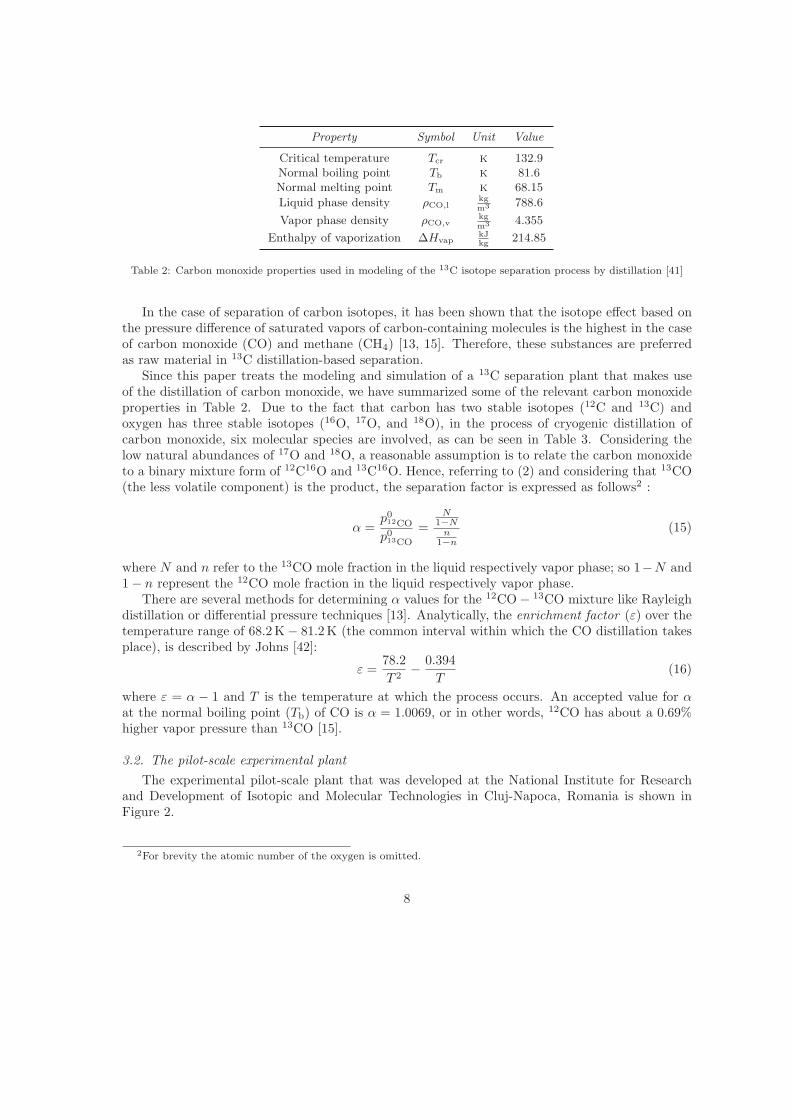
In the case of separation of carbon isotopes, it has been shown that the isotope effect based onthe pressure difference of saturated vapors of carbon-containing molecules is the highest in the caseof carbon monoxide (CO) and methane (CH4) [13, 15]. Therefore, these substances are preferredas raw material in 13C distillation-based separation.

Since this paper treats the modeling and simulation of a 13C separation plant that makes useof the distillation of carbon monoxide, we have summarized some of the relevant carbon monoxideproperties in Table 2. Due to the fact that carbon has two stable isotopes (12C and 13C) andoxygen has three stable isotopes (16O, 17O, and 18O), in the process of cryogenic distillation ofcarbon monoxide, six molecular species are involved, as can be seen in Table 3. Considering thelow natural abundances of 17O and 18O, a reasonable assumption is to relate the carbon monoxideto a binary mixture form of 12C16O and 13C16O. Hence, referring to (2) and considering that 13CO(the less volatile component) is the product, the separation factor is expressed as follows2 :

α =p012CO

p013CO

=N

1−Nn

1−n

(15)

where N and n refer to the 13CO mole fraction in the liquid respectively vapor phase; so 1−N and1− n represent the 12CO mole fraction in the liquid respectively vapor phase.

There are several methods for determining α values for the 12CO− 13CO mixture like Rayleighdistillation or differential pressure techniques [13]. Analytically, the enrichment factor (ε) over thetemperature range of 68.2K− 81.2K (the common interval within which the CO distillation takesplace), is described by Johns [42]:

ε =78.2

T 2−

0.394

T(16)

where ε = α − 1 and T is the temperature at which the process occurs. An accepted value for αat the normal boiling point (Tb) of CO is α = 1.0069, or in other words, 12CO has about a 0.69%higher vapor pressure than 13CO [15].

3.2. The pilot-scale experimental plant

The experimental pilot-scale plant that was developed at the National Institute for Researchand Development of Isotopic and Molecular Technologies in Cluj-Napoca, Romania is shown inFigure 2.

2For brevity the atomic number of the oxygen is omitted.

8

Atomic mass/Molecular mass Natural Abundance(u) (%)

Carbon

12C 12 98.8913C 13 1.11

Oxygen

16O 16 99.7617O 17 0.0418O 18 0.20

Carbon monoxide

12C16O 28 98.652712C17O 29 0.039612C18O 30 0.197813C16O 29 1.107313C17O 30 0.000413C18O 31 0.0022

Table 3: Isotopic forms of carbon, oxygen, and carbon monoxide and their abundances

The distillation column is configurable in several ways, however, in this paper we will considera configuration that consists of one column of 7000mm in height and an inner diameter of 16mmwhich operates in total-reflux regime at a pressure of approximately 0.8 atm. The column is packedwith Heli-Pak stainless steel wire of 1.8×1.8×0.2mm, which has an HETP value of approximately20mm.

Highly purified carbon monoxide is fed up the column, and the extracted waste gas (12COenriched) is taken out from the top of the column, while the 13C enriched product (13CO enriched) iswithdrawn at the base of the column. The vapor stream is ensured by a variable heating resistance(up to 150W) and the total condenser provides the reflux. The condenser uses liquid nitrogenas cooling agent (N2 has a boiling point of Tb=77.3K), and is provided with surface-increasingelements for a better efficiency in the heat exchange between CO vapors and the liquid nitrogen.The cryogenic distillation plant is insulated by a multilayered vacuum jacket. The pressure in thejacket was 8 · 10(−5) torr.

4. Mathematical modeling

The isotope exchange process involving the redistribution of 12C and 13C between the liquidand the vapor phase of the same isotopic compound in physical equilibrium is expressed by [1]:

12CO(liquid) +13CO(vapor) ⇄

13CO(liquid) +12CO(vapor) (17)

In order to derive the mathematical description of the concerned isotope separation process we willproceed as follows. Firstly, based on the two-film theory of the interphase mass transfer, we willderive the rate of transfer of the 13C isotope from the vapor phase to the liquid phase followedby the deriving of the physical description of the overall mass transfer coefficient. From the massbalance relations we will derive the system of equations that governs the evolution of 13C isotope

9

Figure 2: Experimental pilot-scale cryogenic distillation plant with condenser K, primary column C1, final column C2,reboilers B1−B2, vacuum jacket VJ, rough pump RP, diffusion pump DP, temperature sensors T1−T3, manometersM1−M4, level sensors L1−L2, feed reservoir FR, buffer tank BT, waste reservoir WR

with respect to time and height in both the liquid and the vapor phase. Next, we will determinethe volumetric overall mass transfer coefficient as a function of the plant parameters. Finally, wewill solve the system of equations that describe the evolution of 13C isotope with respect to 13COliquid mole fraction.

4.1. The isotopic mass transfer rate

Since the interfacial mass transfer is proportional to the specific interfacial area, an insightfuldescription of the mass transfer rate is the mass transfer rate per unit of volume of transfer device

[35, 43].In the case of our isotope separation process, the specific interfacial area is a property related

to the surface area and to the volume of the column packing. Referring to the general form masstransfer equation (8), and dividing both sides of the relation by the (volume), we obtain:

(mass transfer rate

volume

)

= k × σ × (driving force) (18)

where σ is the specific interfacial area.

10

If τ = mass transfer ratevolume is the rate of transfer of the desired isotope to the enriched phase across

the interface per unit of volume [14], then, in steady state, the isotopic mass flux in terms of molefractions is given by:

τ

σ= kv

(n− n(I)

)(19)

τ

σ= kl

(N(I) −N

)(20)

where n and N represent 13CO mole fractions in the bulk of vapor respectively in the bulk of liquid,while n(I) and N(I) are the vapor and liquid interface mole fractions of 13CO.

Since according to the two-film theory, N(I) and n(I) are in equilibrium, then, with reference to(15):

n(I) =N(I)

α− (α− 1)N(I)(21)

Hence,N(I) − n(I) = n(I)(α− 1)

(1−N(I)

)(22)

By referring to (19), (20), and(22) an expression for τ follows:

τ = K[(n−N) + n(I)(α− 1)

(1−N(I)

)](23)

where1

K=

1

kvσ+

1

klσ(24)

Here, K can be identified with the volumetric overall mass transfer coefficient [35].Due to the fact that in the case of isotope separation, the interfacial concentrations have values

very close to the associated bulk concentrations [14] and thus N(I) ≈ N , n(I) ≈ n, the relation (23)can be rewritten in the following form:

τ = −K[(N − n)− n(α− 1)(1−N)

](25)

For deriving the physical description of the volumetric overall mass transfer coefficient, we referto Fick’s first law of diffusion [20], which states that the mass flux occurs from high-concentrationregions to low-concentration regions, and that it is proportional to the concentration gradient by adiffusion coefficient:

JA = −D∇cA (26)

where JA is the molar flux, D is the molecular diffusivity, and ∇cA is the gradient of molar con-centration of component A. In one spatial dimension3 (26) becomes:

JA = −D∂cA∂z

(27)

where z represents the position.

3Since the mass transfer device in the case of isotope separation by cryogenic distillation is usually a very longcolumn with a small diameter, a good approximation arises by considering only the longitudinal effects (in our casethe column is 7000mm in length and 16mm in diameter).

11

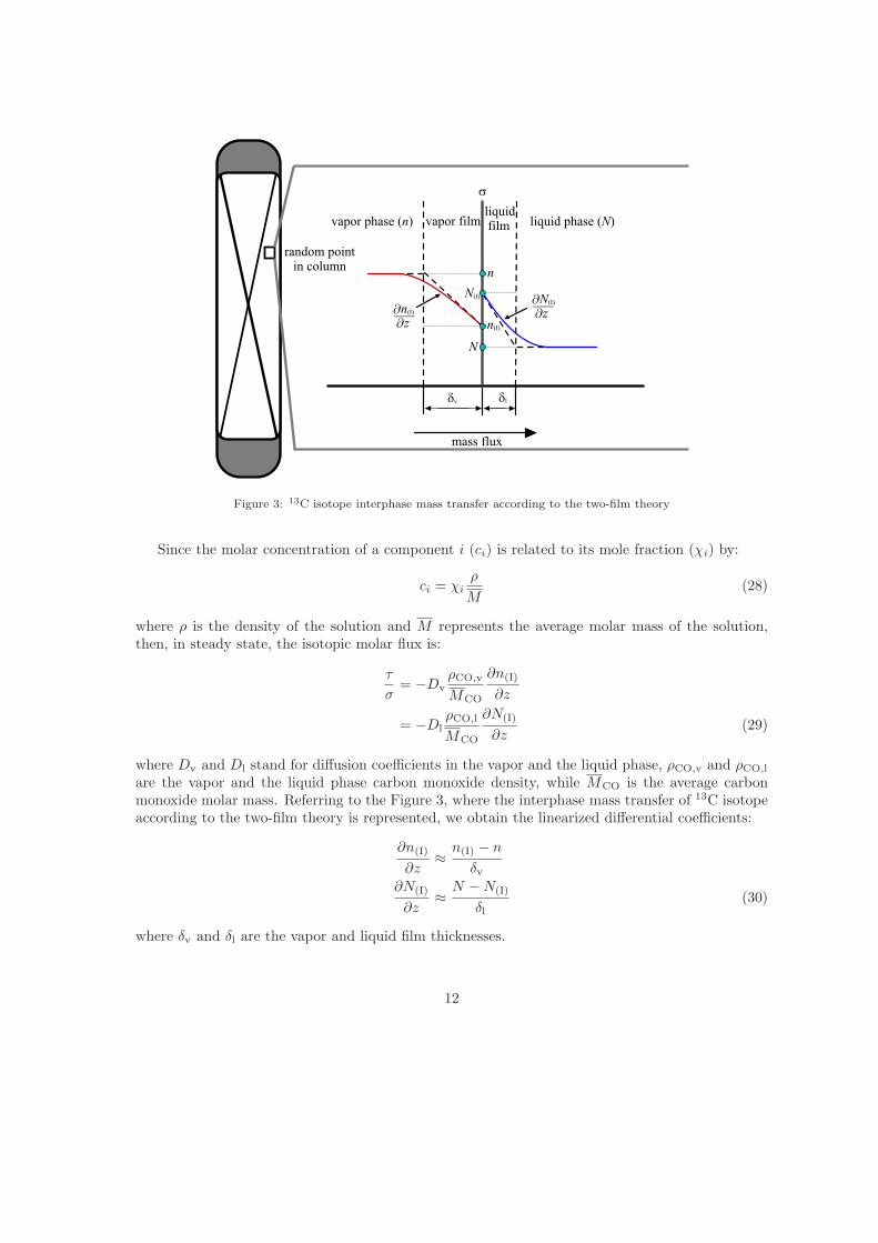
Figure 3: 13C isotope interphase mass transfer according to the two-film theory

Since the molar concentration of a component i (ci) is related to its mole fraction (χi) by:

ci = χi

ρ

M(28)

where ρ is the density of the solution and M represents the average molar mass of the solution,then, in steady state, the isotopic molar flux is:

τ

σ= −Dv

ρCO,v

MCO

∂n(I)

∂z

= −DlρCO,l

MCO

∂N(I)

∂z(29)

where Dv and Dl stand for diffusion coefficients in the vapor and the liquid phase, ρCO,v and ρCO,l

are the vapor and the liquid phase carbon monoxide density, while MCO is the average carbonmonoxide molar mass. Referring to the Figure 3, where the interphase mass transfer of 13C isotopeaccording to the two-film theory is represented, we obtain the linearized differential coefficients:

∂n(I)

∂z≈

n(I) − n

δv∂N(I)

∂z≈

N −N(I)

δl(30)

where δv and δl are the vapor and liquid film thicknesses.

12

From (29) and (30) the physical description of the volumetric overall mass transfer coefficientfollows:

1

K=

1

σ

MCOδvDvρCO,v

+1

σ

MCOδlDlρCO,l

(31)

4.2. The isotopic mass balance equations

For determining the isotopic mass balance equations we will consider a column element as shownin Figure 4(a). The column element, of height dz and diameter d, lies between heights z and z+dz.In the figure, L and V are the liquid and vapor molar flow rates of the 12CO and 13CO mixture percross section area of the column (Ac), while L13CO and V13CO denote the 13CO liquid and vapormolar flow rates. At height z, the liquid molar flow rate L13CO(z, t) is entering the column element,while the vapor molar flow rate V13CO(z, t) is leaving the column element. At height z + dz, theliquid and the vapor molar flow rates are leaving, respectively entering the column element. Sincethe heavy isotope is accumulating in the liquid phase the height will be measured by convention inthe liquid flow direction.

If νL13CO(z, t) is the number of 13CO moles in the liquid phase that are entering the column

element between t and t + dt, then the 13CO liquid molar flow rate at height z per cross sectionarea of the column is defined by:

L13CO(z, t) =νL13CO

(z, t)

Acdt(32)

Analogously, the 13CO vapor molar flow rate at height z is defined by:

V13CO(z, t) =νV13CO

(z, t)

Acdt(33)

Recalling the notions presented in Section 4.1, the number of moles transferred from the vaporphase to the liquid phase (ντ ), in the volume dv = Acdz, in the time between t and t+dt, is definedby:

ντ = τdvdt (34)

At time t in the column element there is a certain number of 13CO moles referred to as 13COhold-up.

Figure 4(b) emphasizes the time evolution of the 13CO hold-up per volume element in the liquid(H13CO,l) and in the vapor phase (H13CO,v). The liquid 13CO hold-up in the column element, attime t is defined by:

H13CO,l(z, t) =νH13CO,l

(z, t)

dv(35)

where νH13CO,l(z, t) is the number of 13CO moles in the column element in the liquid phase at time

t. Analogously, the vapor 13CO hold-up per column element is defined by:

H13CO,v(z, t) =νH13CO,v

(z, t)

dv(36)

Since no chemical reaction takes place, the isotopic mass balance for the liquid phase, in thecolumn element, in the time span between t and t + dt, is described in terms of number of molesby:

(νL13CO(z, t) + ντ )

︸ ︷︷ ︸

mass in

− νL13CO(z + dz, t)

︸ ︷︷ ︸

mass out

= νH13CO,l(z, t+ dt)− νH13CO,l

(z, t)︸ ︷︷ ︸

accumulation

(37)

13

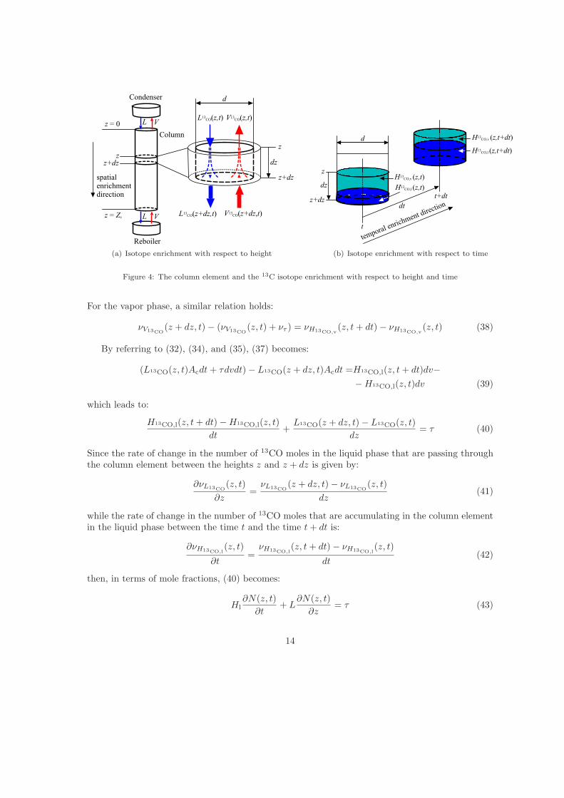
(a) Isotope enrichment with respect to height (b) Isotope enrichment with respect to time

Figure 4: The column element and the 13C isotope enrichment with respect to height and time

For the vapor phase, a similar relation holds:

νV13CO(z + dz, t)− (νV13CO

(z, t) + ντ ) = νH13CO,v(z, t+ dt)− νH13CO,v

(z, t) (38)

By referring to (32), (34), and (35), (37) becomes:

(L13CO(z, t)Acdt+ τdvdt)− L13CO(z + dz, t)Acdt =H13CO,l(z, t+ dt)dv−

−H13CO,l(z, t)dv (39)

which leads to:

H13CO,l(z, t+ dt)−H13CO,l(z, t)

dt+

L13CO(z + dz, t)− L13CO(z, t)

dz= τ (40)

Since the rate of change in the number of 13CO moles in the liquid phase that are passing throughthe column element between the heights z and z + dz is given by:

∂νL13CO(z, t)

∂z=

νL13CO(z + dz, t)− νL13CO

(z, t)

dz(41)

while the rate of change in the number of 13CO moles that are accumulating in the column elementin the liquid phase between the time t and the time t+ dt is:

∂νH13CO,l(z, t)

∂t=

νH13CO,l(z, t+ dt)− νH13CO,l

(z, t)

dt(42)

then, in terms of mole fractions, (40) becomes:

Hl∂N(z, t)

∂t+ L

∂N(z, t)

∂z= τ (43)

14

where Hl is the12CO and 13CO (i.e. the raw material) hold-up in the liquid phase and L is the liquid

molar flow rate per cross section area of the column of the 12CO and 13CO mixture. Analogously,for the vapor phase, the following relation holds:

Hv∂n(z, t)

∂t− V

∂n(z, t)

∂z= −τ (44)

The relations (43) and (44) describe the rate of change of the heavy isotope (i.e. the product)in time and height, in the liquid and vapor phase, with respect to associated plant variables, Hl,Hv, L, V , and τ .

4.3. The volumetric overall mass transfer coefficient

The volumetric overall mass transfer coefficient is related to physical properties like moleculardiffusivity and vapor and liquid-phase film thickness, which are very difficult to measure [20, 19].However, in the following we will estimate the value of the mass transfer coefficient, based on theplant parameters by referring to the isotopic mass balance relations (43), (44) and to the rate oftransfer per unit volume defined by (25).

At steady state, (43) and (44) become4:

LdN

dz= −K

[(N − n)− n(α− 1)(1−N)

](45)

−Vdn

dz= K

[(N − n)− n(α− 1)(1−N)

](46)

When no withdrawal is performed, and thus the liquid is converted entirely into vapor, thecolumn being operated in total-reflux regime, the isotopic mole fractions are equal at the ends ofthe column, and in addition, the internal streams are equal:

N(z = Zc) = n(z = Zc)

L = V (47)

N(z = 0) = n(z = 0)

Therefore, the steady-state relations (45) and (46) are reduced to:

LdN

dz= K(α− 1)N(1−N) (48)

If we denote by λ the term K(α−1)L

, it can be easily observed that the relation is similar to theVerhulst-Pearl logistic equation, which describes the population growth in an environment withlimited resources [44]:

dN

dz= λN

(

1−N

µ

)

(49)

4For the sake of brevity we will not explicitly put z as argument for N and n

15

where λ represents the intrinsic growth rate and µ is the saturation level, with the growth takingplace not in time, but in space. Since the growth applies to mole fractions the saturation level isequal to unity. Thus, the solution of (49) is:

N(z) =eλzγ

1 + eλzγ(50)

where γ is a constant of integration that can be determined from the initial condition. Therefore,the 13C enrichment in the liquid phase with respect to the height follows:

N(z) =1

1 +

(

1−N0

N0

)

e−K(α−1)z

L

(51)

where N0 stands for natural 13C isotopic abundance.The overall volumetric mass transfer coefficient K may now be determined from (51), written

for the boundary condition (z = Zc), and it is equal to:

K =L

(α− 1)Zcln

( N(Zc)1−N(Zc)

N0

1−N0

)

(52)

4.4. The isotope separation partial differential equations

The system of Partial Differential Equations (PDEs) (43)-(44) can be solved in terms of the13CO liquid mole fraction (N), by describing the 13CO vapor mole fraction (n) from (25) and (43)as:

n =Hl

K∂N∂t

+ LK

∂N∂z

+N

1 + (α− 1)(1−N)(53)

and computing its partial derivatives with respect to time and height:

∂n

∂t=

(

Hl

K∂2N∂t2

+ LK

∂2N∂t∂z

+ ∂N∂t

)

A+ ∂N∂t

(α− 1)B

A2(54)

∂n

∂z=

(

Hl

K∂2N∂z∂t

+ LK

∂2N∂z2 + ∂N

∂z

)

A+ ∂N∂z

(α− 1)B

A2(55)

where A =[1 + (α− 1)(1−N)

]and B =

(

Hl

K∂N∂t

+ LK

∂N∂z

+N

)

.

From the relations set (43), (44), (53), (54), (55) we obtain the following PDE:

∂2N

∂t2

(AHvHl

K

)

+∂N

∂t

[AHv +BHv(α− 1) +A2Hl

]=

=∂2N

∂z∂t

[

A

(V Hl

K−

LHv

K

)]

+∂2N

∂z2

(ALV

K

)

+∂N

∂z

[AV +BV (α− 1)−A2L

](56)

where we took into account Young’s Theorem on the equality of mixed partial derivatives [45]. Inthe following, (56) will be referred to as the full nonlinear isotope separation PDE model.

16

However, knowing that the concentration varies very slowly due to the low enrichment factor(i.e. ε = α − 1 ≈ 0.0069 [13, 15]) and that the steady-state regime is achieved after several daysonly, one can neglect the second-order derivative in time, the mixed derivatives, and the termscontaining ∂N

∂t(α− 1) and ∂N

∂z(α− 1)B.

After these simplifications and knowing that the bottom product flow rate in the column (Ψ) isgiven by Ψ = L− V , the following PDE follows:

(Hl +Hv)∂N

∂t=

(LV

K

)∂2N

∂z2−

∂N

∂z

[Ψ+ L(α− 1)(1−N)

](57)

and it will be referred as the quasi-linear isotope separation PDE model.The general form of (57):

c6∂N

∂t= c5

∂2N

∂s2−

∂

∂s

[ΨN + c1N(1−N)

](58)

where c6, c5, Ψ, and, c1 are constants, is referred to in [14] as the fundamental equation of isotopeseparation.

Since the 13CO liquid phase mole fraction N ≪ 1, (57) may be furthermore simplified to thefollowing form:

(Hl +Hv)∂N

∂t=

(LV

K

)∂2N

∂z2−

∂N

∂z

[Ψ+ L(α− 1)

](59)

which will be referred to as the linear isotope separation PDE model.

5. Numerical analysis

Previously we have determined the full nonlinear isotope separation PDE model (56) and basedon certain assumptions we have derived two simplified models, a quasi-linear (57) and a linearmodel (59). In this section we will proceed with numerical analysis issues in order to numericallysolve and simulate these models.

For obtaining a finite-dimensional system of difference equations or ordinary differential equa-tions to numerically solve a PDE one can consider methods like finite-difference, finite-element,finite-volume, or weighted-residual methods [25, 46, 30]. In the case of a problem with a simplegeometry finite-difference and spectral methods are suitable choices [25]. For problems with a com-plex geometry or complicated boundary conditions one can chose finite-element or finite-volumemethods [47, 30].

Since the main advantage of the finite-difference methods is the flexibility in dealing with non-linear problems and since in addition they are easy to implement [30, 48], we will choose thefinite-difference method for analysis of the three models.

As is well known, for a numerical method, consistency, stability, and convergence are the mostimportant aspects [30]. As a reminder, a finite-difference equation is consistent if the truncationerror approaches zero (this is usually the case for finite-difference approximations derived fromTaylor series), it is stable if the error remains uniformly bounded, and it is convergent if its solutionapproaches that of the partial differential equation as the grid size approaches zero [30, 48].

Let the 13CO liquid mole fraction function N(z, t) be identified with u(i, j). The two integerindices i and j indicates where the quantity is evaluated and are related to the Cartesian coordinates

17

as follows:

z(i) = z0 + i∆z

t(j) = t0 + j∆t

The grid has a fixed mesh spacing ∆z in the z-direction and ∆t in the t-direction. Considering theexpansions in Taylor series around a point (z(i), t(j)) [30], the forward-difference approximation for∂N∂z

and ∂N∂t

at the coordinates (z(i), t(j)) is:

∂N

∂z= uz(i, j) ≈

u(i+ 1, j)− u(i, j)

∆z(60)

∂N

∂t= ut(i, j) ≈

u(i, j + 1)− u(i, j)

∆t(61)

where ∆z and ∆t represent the grid size in the height and in the time dimension.The backward-difference approximation for ∂N

∂tis given by:

∂N

∂t= ut(i, j) ≈

u(i, j)− u(i, j − 1)

∆t(62)

The second-order central difference for ∂2N∂z2 and ∂2N

∂t2are given by:

∂2N

∂z2= uzz(i, j) ≈

u(i+ 1, j)− 2u(i, j) + u(i− 1, j)

(∆z)2(63)

∂2N

∂t2= utt(i, j) ≈

u(i, j + 1)− 2u(i, j) + u(i, j − 1)

(∆t)2(64)

Finally, the mixed derivative ∂2N∂z∂t

approximation is given by:

∂2N

∂z∂t= uzt(i, j) ≈

u(i, j)− u(i− 1, j)− u(i, j − 1) + u(i− 1, j − 1)

∆z∆t(65)

Using (60)−(65) we will numerically solve the PDE models (56), (57), and (59)The time-space domain of our distributed parameter system is determined by the duration of

the total-reflux experiment and by the length of the column. The initial condition is represented bythe natural abundance of 13C, while the boundary conditions are determined by the concentrationachieved at the top of the column (z = 0) respectively at the bottom of the column (z = Zc).

During the total-reflux experiment, samples were collected from both ends of the column every 12hours (see Figure 5). The plant operated in total-reflux regime for 96 hours and the electrical powerthat supplied the heating resistance was 30W. The two curves shown in Figure 5 representing theboundary conditions used in numerical analysis were obtained by the use of a fifth-order polynomialinterpolation that fits the data in a least-squares sense.

Since this experiment was conducted in the total-reflux regime, the vapor and liquid internalstreams were equal (L = V ). The vapor internal stream was determined by knowing the electricalpower which supplied the heating resistance and the heat transfer through the multilayered vacuumjacket [49], [50] used for insulation.

18

0 12 24 36 48 60 72 84 960

0.29

1.11

2.623

3

time (h)

13C

conce

ntr

atio

n (

%)

bottom sample composition

top sample composition

top experimental data interpolating polynomial

bottom experimental data interpolating polynomial

Figure 5: 13C concentrations achieved by the pilot-scale experimental plant

The total hold-up in the column (Htot = Hl +Hv) was determined by measuring the quantityof raw material fed to the column during the operations prior to the beginning of the experiment.The vapor phase hold-up (Hv) was determined by measuring the electrical power which suppliedthe heating resistance and knowing the heat received through the multilayered vacuum jacket usedfor insulation. Hence, the liquid phase hold-up (Hl) was determined by:

Hl = Htot −Hv (66)

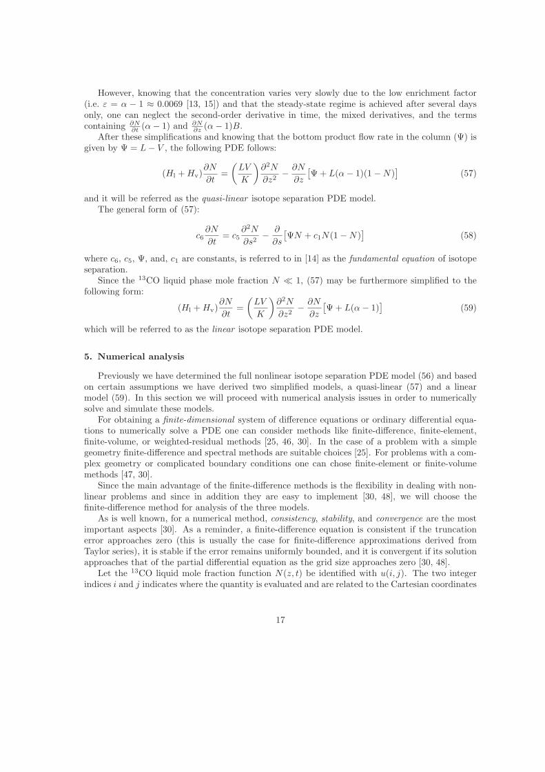
6. Results and discussion

In the case of linear PDEs, for a well-posed initial-value problem and a consistent finite-differencescheme, the Lax equivalence theorem applies [29], stability being the necessary and sufficient con-dition for convergence. Therefore, we have used the linear PDE model (59) as reference model forthe convergence of the solution. However, for all the schemes used in the simulations, wheneverthe stability was achieved, the full nonlinear (56) and the quasi-linear model (57) were convergenttoo. This fact is not surprising at all since the nonlinear terms are close to zero, thus confirmingthe assumptions made in Section 4.4.

Figures 6(a) and 6(b) show the 13CO mole fraction distribution in the column with respect toboth height and time. The isotope distribution was obtained by simulating the full nonlinear model(56) for 50 discretization divisions applied to the space domain (i.e. ∆z = 7

50m) and a time step(∆t) equal to 0.5 seconds. In order to compare the isotope separation process models, for the samemesh spacing, we simulated the linear and the quasi-linear models. The simulation time of the

19

0 1 2 3 4 5 6 7

012243648607284960

0.29

1.11

2.6233

height (m)time (h)

13C

conce

ntr

atio

n (

%)

0.29

1.11

2.623

(a) 13C isotope concentration distribution

height (m)

tim

e(h

)

0 1 2 3 4 5 6 70

12

24

36

48

60

72

84

9696

0.29

1.11

2.623

(b) 13C isotope concentration distribution (contour view)

Figure 6: 13C isotope concentration distribution with respect to time and height

0 1 2 3 4 5 6 7

012243648607284960

2

4

67

x 10−3

height (m)time (h)

Rel

ativ

eer

ror

0

1

2

3

4

5

6x 10

−3

(a) Relative error of the linear model

0 1 2 3 4 5 6 7

012

2436

4860

7284

960

2

4

5

7

x 10−3

height (m)time (h)

Rel

ativ

eer

ror

0

1

2

3

4

5

6x 10

−3

(b) Relative error of the quasi-linear model

Figure 7: Relative errors of the linear and quasi-linear models

linear model was approximately 16.5 seconds, while the simulation time of the quasi-linear modelwas approximately 17 seconds. The simulation time of the full nonlinear model was 5 minutes and10 seconds.

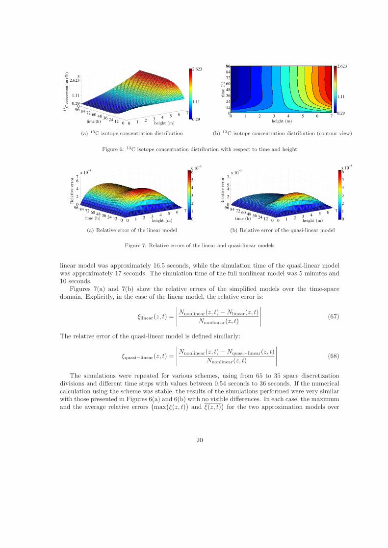
Figures 7(a) and 7(b) show the relative errors of the simplified models over the time-spacedomain. Explicitly, in the case of the linear model, the relative error is:

ξlinear(z, t) =

∣∣∣∣∣

Nnonlinear(z, t)−Nlinear(z, t)

Nnonlinear(z, t)

∣∣∣∣∣

(67)

The relative error of the quasi-linear model is defined similarly:

ξquasi−linear(z, t) =

∣∣∣∣∣

Nnonlinear(z, t)−Nquasi−linear(z, t)

Nnonlinear(z, t)

∣∣∣∣∣

(68)

The simulations were repeated for various schemes, using from 65 to 35 space discretizationdivisions and different time steps with values between 0.54 seconds to 36 seconds. If the numericalcalculation using the scheme was stable, the results of the simulations performed were very similarwith those presented in Figures 6(a) and 6(b) with no visible differences. In each case, the maximumand the average relative errors

(max

(ξ(z, t)

)and ξ(z, t)

)for the two approximation models over

20

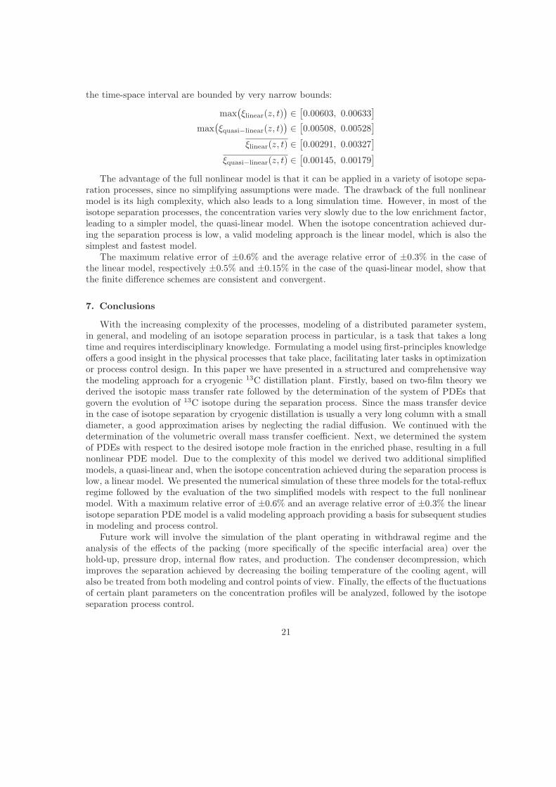
the time-space interval are bounded by very narrow bounds:

max(ξlinear(z, t)

)∈[0.00603, 0.00633

]

max(ξquasi−linear(z, t)

)∈[0.00508, 0.00528

]

ξlinear(z, t) ∈[0.00291, 0.00327

]

ξquasi−linear(z, t) ∈[0.00145, 0.00179

]

The advantage of the full nonlinear model is that it can be applied in a variety of isotope sepa-ration processes, since no simplifying assumptions were made. The drawback of the full nonlinearmodel is its high complexity, which also leads to a long simulation time. However, in most of theisotope separation processes, the concentration varies very slowly due to the low enrichment factor,leading to a simpler model, the quasi-linear model. When the isotope concentration achieved dur-ing the separation process is low, a valid modeling approach is the linear model, which is also thesimplest and fastest model.

The maximum relative error of ±0.6% and the average relative error of ±0.3% in the case ofthe linear model, respectively ±0.5% and ±0.15% in the case of the quasi-linear model, show thatthe finite difference schemes are consistent and convergent.

7. Conclusions

With the increasing complexity of the processes, modeling of a distributed parameter system,in general, and modeling of an isotope separation process in particular, is a task that takes a longtime and requires interdisciplinary knowledge. Formulating a model using first-principles knowledgeoffers a good insight in the physical processes that take place, facilitating later tasks in optimizationor process control design. In this paper we have presented in a structured and comprehensive waythe modeling approach for a cryogenic 13C distillation plant. Firstly, based on two-film theory wederived the isotopic mass transfer rate followed by the determination of the system of PDEs thatgovern the evolution of 13C isotope during the separation process. Since the mass transfer devicein the case of isotope separation by cryogenic distillation is usually a very long column with a smalldiameter, a good approximation arises by neglecting the radial diffusion. We continued with thedetermination of the volumetric overall mass transfer coefficient. Next, we determined the systemof PDEs with respect to the desired isotope mole fraction in the enriched phase, resulting in a fullnonlinear PDE model. Due to the complexity of this model we derived two additional simplifiedmodels, a quasi-linear and, when the isotope concentration achieved during the separation process islow, a linear model. We presented the numerical simulation of these three models for the total-refluxregime followed by the evaluation of the two simplified models with respect to the full nonlinearmodel. With a maximum relative error of ±0.6% and an average relative error of ±0.3% the linearisotope separation PDE model is a valid modeling approach providing a basis for subsequent studiesin modeling and process control.

Future work will involve the simulation of the plant operating in withdrawal regime and theanalysis of the effects of the packing (more specifically of the specific interfacial area) over thehold-up, pressure drop, internal flow rates, and production. The condenser decompression, whichimproves the separation achieved by decreasing the boiling temperature of the cooling agent, willalso be treated from both modeling and control points of view. Finally, the effects of the fluctuationsof certain plant parameters on the concentration profiles will be analyzed, followed by the isotopeseparation process control.

21

Acknowledgements

This paper was supported by the project ”Doctoral studies in engineering sciences for devel-oping the knowledge based society-SIDOC” contract no. POSDRU/88/1.5/S/60078, projectco-funded from European Social Fund through Sectorial Operational Program Human Re-sources 2007-2013. The work was supported as well by CNCSIS-UEFISCDI, project number630 PNII-IDEI code 228/2008.

References

[1] W.G. Mook. Abundance and fractionation of stable isotopes. In W.G. Mook, editor, Environ-mental Isotopes in the Hydrological Cycle. Principles and Applications, volume 1, chapter 3,pages 31–48. UNESCO Publishing, Paris, 2000.

[2] G. Faure and T.M. Mensing. Isotopes. Principles and Applications. John Wiley and Sons,Hoboken, third edition, 2005.

[3] R.A. de Vries, M. de Bruin, J.J. Marx, and A. Van de Wiel. Radioisotopic labels for blood cellsurvival studies: a review. Nuclear Medicine and Biology, 20(7):809–817, 1993.

[4] P.A. de Groot. Carbon. In P.A. de Groot, editor, Handbook of Stable Isotope Analytical

Techniques, volume 2, chapter 4, pages 229–329. Elsevier, Amsterdam, first edition, 2009.

[5] P. Ciais, P.P. Tans, M. Trolier, J.W.C. White, and R.J. Francey. A large norhern hemi-sphere terrestrial CO2 sink indicated by the 13C/12C ratio of atmospheric CO2. Science,269(5227):1098–1102, 1995.

[6] J. Bigeleisen. Chemistry of isotopes. Science, 147(3657):463–471, 1965.

[7] P.A. de Groot. Isotope separation methods. In P.A. de Groot, editor, Handbook of Stable

Isotope Analytical Techniques, volume 2, chapter 20, pages 1025–1032. Elsevier, Amsterdam,first edition, 2009.

[8] W.A. Van Hook. Isotope separation. In A. Vertes, S. Nagy, and Z. Klencsar, editors, Hand-book of Nuclear Chemistry, volume 5, chapter 5, pages 177–211. Kluwer Academic Publishers,Dordrecht, 2003.

[9] H. London. Separation of Isotopes. George Newnes Limited, London, 1961.

[10] OECD/Nuclear Energy Agency. Beneficial Uses and Production of Isotopes. OECD Publishing,Paris, 2005.

[11] H.C. Urey. The thermodynamic properties of isotopic substances. Journal of the Chemical

Society, pages 562–581, 1947.

[12] J. Bigeleisen and M.G. Mayer. Calculation of equilibrium constants for isotopic exchangereactions. The Journal of Chemical Physics, 15(5):261–267, 1947.

[13] G. Jancso and W.A. Van Hook. Condensed phase isotope effects (especially vapor pressureisotope effects). Chemical Reviews, 74(6):689–750, 1974.

22

[14] K.P. Cohen. The Theory of Isotope Separation as Applied to the Large-Scale Production of

U235, volume 1B of National Nuclear Energy Series, Manhattan Project Technical Section,

Division III. McGraw-Hill, New York, first edition, 1951.

[15] B.M. Andreev, E.P. Magomedbekov, A.A. Raitman, M.B. Pozenkevich, Yu.A. Sakharovsky,and A.V. Khoroshilov. Separation of Isotopes of Biogenic Elements in Two-phase Systems.Elsevier, Amsterdam, 2007.

[16] B.B. McInteer. Isotope separation by distillation: Design of a carbon-13 plant. Separation

Science and Technology, 15(3):491–508, 1980.

[17] H.-L. Li, Y.-L. Ju, L.-J. Li, and D.-G. Xu. Separation of isotope 13C using high-performancestructured packing. Chemical Engineering and Processing: Process Intensification, 49(3):255–261, 2010.

[18] E.-H. Dulf, C. Festila, and F. Dulf. Monitoring and control system of a separation columnfor 13C enrichment by cryogenic distillation of carbon monoxide. International Journal of

Mathematical Models and Methods in Applied Sciences, 3(3):196–203, 2009.

[19] E.L. Cussler. Diffusion. Mass Transfer in Fluid Systems. Cambridge University Press, Cam-bridge, third edition, 2009.

[20] C.J. King. Separation Processes. McGraw-Hill, New York, second edition, 1980.

[21] S. Skogestad. Dynamics and control of distillation columns: A tutorial introduction. Chemical

Engineering Research and Design, 75(6):539–562, 1997.

[22] I.J. Halvorsen and S. Skogestad. Theory of Distillation. In I.D. Wilson, E.R. Adlard, M. Cooke,and C.F. Poole, editors, Encyclopedia of Separation Science, pages 1117–1134. Academic Press,San Diego, 2000.

[23] S. Skogestad. Plantwide control: the search for the self-optimizing control structure. Journal

of Process Control, 10(5):487–507, 2000.

[24] M.F. Sagfors and K.V. Waller. Multivariable control of ill-conditioned distillation columnsutilizing process knowledge. Journal of Process Control, 8(3):197–208, 1998.

[25] H.-X. Li and C. Qi. Modeling of distributed parameter systems for applications - a synthesizedreview from time-space separation. Journal of Process Control, 20(8):891–901, 2010.

[26] C. Qi, H.-T. Zhang, and H.-X. Li. A multi-channel spatio-temporal Hammerstein modelingapproach for nonlinear distributed parameter processes. Journal of Process Control, 19(1):85–99, 2009.

[27] R. Curtain and K. Morris. Transfer functions of distributed parameter systems: A tutorial.Automatica, 45(5):1101–1116, 2009.

[28] L. Debnath. Nonlinear Partial Differential Equations for Scientists and Engineers. Birkhauser,Boston, second edition, 2005.

[29] P.D. Lax and R.D. Richtmyer. Survey of the stability of linear finite difference equations.Communications on Pure and Applied Mathematics, 9:267–293, 1956.

23

[30] T.J. Chung. Computational Fluid Dynamics. Cambridge University Press, Cambridge, secondedition, 2010.

[31] J.C. Strikwerda. Finite Difference Schemes and Partial Differential Equations. SIAM: Societyfor Industrial and Applied Mathematics, Philadelphia, second edition, 2004.

[32] K.T. Chuang and K. Nandakumar. Tray columns: Design. In I.D. Wilson, E.R. Adlard,M. Cooke, and C.F. Poole, editors, Encyclopedia of Separation Science, pages 1135–1140.Academic Press, San Diego, 2000.

[33] L. Klemas and J.A. Bonilla. Packed Columns: Design and Performance. In I.D. Wilson,E.R. Adlard, M. Cooke, and C.F. Poole, editors, Encyclopedia of Separation Science, pages1081–1098. Academic Press, San Diego, 2000.

[34] P. Wankat. Separation Process Engineering. Prentice Hall, Upper Saddle River, second edition,2006.

[35] R.F. Strigle, Jr. Packed Tower Design and Applications: Random and Structured Packings.Gulf Publishing Company, Houston, second edition, 1994.

[36] M.R. Fenske. Fractionation of straight-run pennsylvania gasoline. Industrial and Engineering

Chemistry, 24(5):482–485, 1932.

[37] D. Azbel. Two-Phase Flows in Chemical Engineering. Cambridge University Press, Cambridge,1981.

[38] J.R. Taricska, J.P. Chen, Y.-T. Hung, L.K. Wang, and S.-W. Zou. Surface and spray aeration.In L.K. Wang, N.C. Pereira, and Y-T Hung, editors, Handbook of Environmental Engineering,volume 8, pages 157–165. Humana Press, New York, 2009.

[39] F.M. Khoury. Multistage Separation Processes, chapter 15, pages 389–410. CRC Press, BocaRaton, third edition, 2005.

[40] J.A. Mandler. Modelling for control analysis and design in complex industrial separation andliquefaction processes. Journal of Process Control, 10(2-3):167–175, 2000.

[41] Air Liquide Group. Physical properties of gases, safety, MSDS, enthalpy, material compati-

bility, gas liquid equilibrium, density, viscosity, flammability, transport properties, 2011 (lastaccessed June 9, 2011). http://encyclopedia.airliquide.com.

[42] T.F. Johns. Vapor pressure ratio of 12C16O and 13C16O. Proceedings of the Physical Society.

Section B, 66(9):808–809, 1953.

[43] J. Niessner and S.M. Hassanizadeh. Modeling kinetic interphase mass transfer for two-phase flow in porous media including fluid-fluid interfacial area. Transport in Porous Media,80(2):329–344, 2009.

[44] A. Tsoularis and J. Wallace. Analysis of logistic growth models. Mathematical Biosciences,179(1):21–55, 2002.

[45] W.H. Young. On the conditions for the reversibility of the order of partial differentiation.Proceedings Royal Society of Edinburgh, 29:136–164, 1908-1909.

24

[46] H.-X. Li, C. Qi, and Y. Yu. A spatio-temporal Volterra modeling approach for a class ofdistributed industrial processes. Journal of Process Control, 19(7):1126–1142, 2009.

[47] D.S. Burnett. Finite Element Analysis: from Concepts to Applications. Addison-Wesley,Reading, 1987.

[48] J.H. Mathews and K.D. Fink. Numerical Methods using MATLAB. Prentice Hall, UpperSaddle River, third edition, 1999.

[49] S. Jacob, S. Kasthurirengan, and R. Karunanithi. Investigations into the thermal performanceof multilayer insulation (300-77K) Part 1: Calorimetric studies. Cryogenics, 32(12):1137–1146,1992.

[50] S. Jacob, S. Kasthurirengan, and R. Karunanithi. Investigations into the thermal performanceof multilayer insulation (300-77K) Part 2: Thermal analysis. Cryogenics, 32(12):1147–1153,1992.

25