Modeling, Analysis and Simulation for Degenerate Dipolar Quantum Gas

Weizhu Bao Department of Mathematics

& Center for Computational Science and Engineering National University of Singapore

Email: bao@math.nus.edu.sg URL: http://www.math.nus.edu.sg/~bao

Collaborators: Y. Cai (Postdoc, NUS), M. Rosenkranz (Postdoc, NUS), N. Ben Abdallah (UPS, France), Z. Lei (Fudan University, China), H. Wang (Yunan Univ. Economics and Finance, China & NUS)

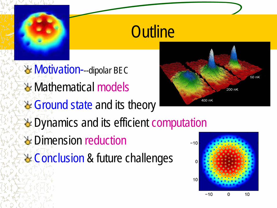
Outline

Motivation---dipolar BEC

Mathematical models Ground state and its theory Dynamics and its efficient computation Dimension reduction Conclusion & future challenges

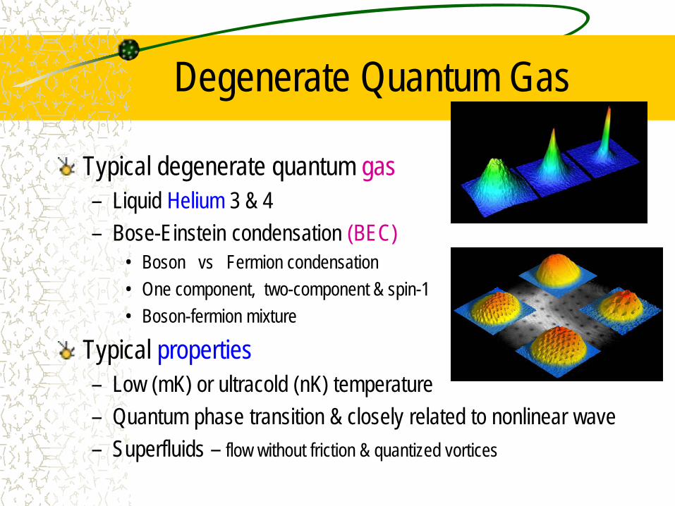
Degenerate Quantum Gas

Typical degenerate quantum gas – Liquid Helium 3 & 4 – Bose-Einstein condensation (BEC)

• Boson vs Fermion condensation • One component, two-component & spin-1 • Boson-fermion mixture

Typical properties – Low (mK) or ultracold (nK) temperature – Quantum phase transition & closely related to nonlinear wave – Superfluids – flow without friction & quantized vortices

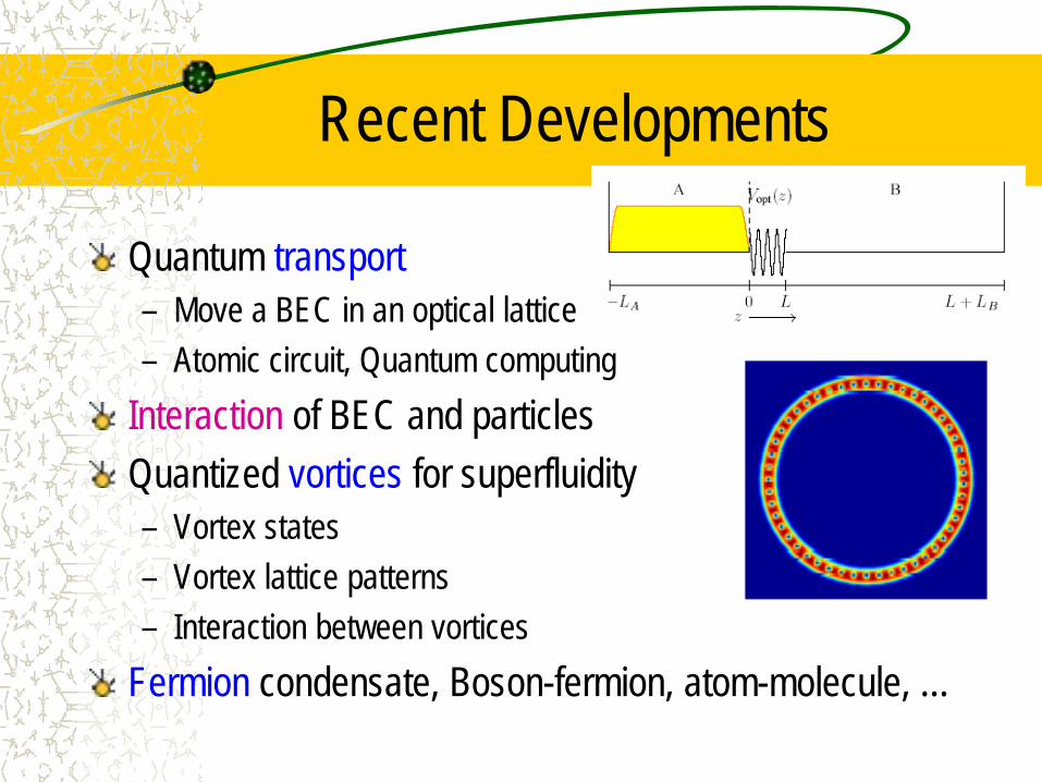
Recent Developments

Quantum transport – Move a BEC in an optical lattice – Atomic circuit, Quantum computing

Interaction of BEC and particles Quantized vortices for superfluidity – Vortex states – Vortex lattice patterns – Interaction between vortices

Fermion condensate, Boson-fermion, atom-molecule, …

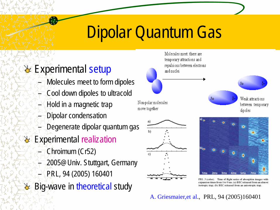
Dipolar Quantum Gas

Experimental setup – Molecules meet to form dipoles – Cool down dipoles to ultracold – Hold in a magnetic trap – Dipolar condensation – Degenerate dipolar quantum gas

Experimental realization – Chroimum (Cr52) – 2005@Univ. Stuttgart, Germany – PRL, 94 (2005) 160401

Big-wave in theoretical study A. Griesmaier,et al., PRL, 94 (2005)160401

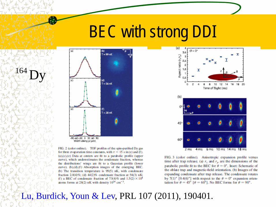
BEC with strong DDI

Lu, Burdick, Youn & Lev, PRL 107 (2011), 190401.

164 Dy

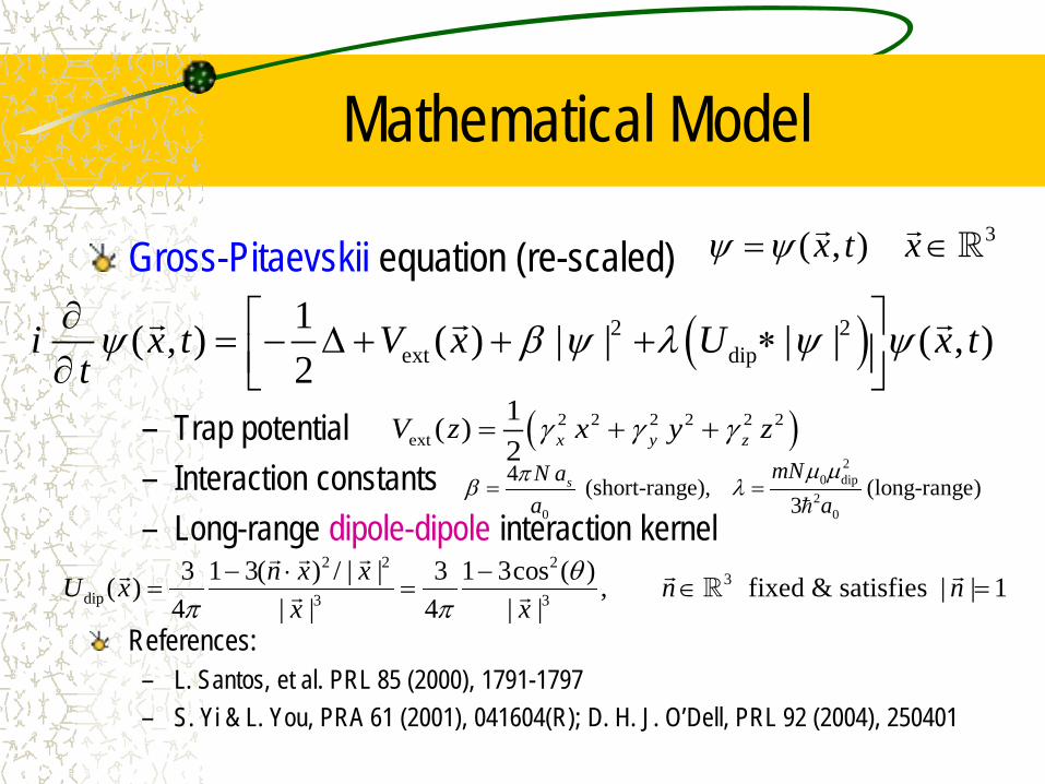
Mathematical Model

Gross-Pitaevskii equation (re-scaled) – Trap potential – Interaction constants – Long-range dipole-dipole interaction kernel

References:

– L. Santos, et al. PRL 85 (2000), 1791-1797 – S. Yi & L. You, PRA 61 (2001), 041604(R); D. H. J. O’Dell, PRL 92 (2004), 250401

( )2 2ext dip

1( , ) ( ) | | | | ( , )2

i x t V x U x ttψ β ψ λ ψ ψ∂ = − ∆ + + + ∗ ∂

3( , )x t xψ ψ= ∈

( )2 2 2 2 2 2ext

1( )2 x y zV z x y zγ γ γ= + +

20 dip

20 0

4 (short-range), (long-range)3

s mNN aa a

µ µπβ λ= =

2 2 23

dip 3 33 1 3( ) / | | 3 1 3cos ( )( ) , fixed & satisfies | | 1

4 | | 4 | |n x xU x n n

x xθ

π π− ⋅ −

= = ∈ =

Mathematical Model

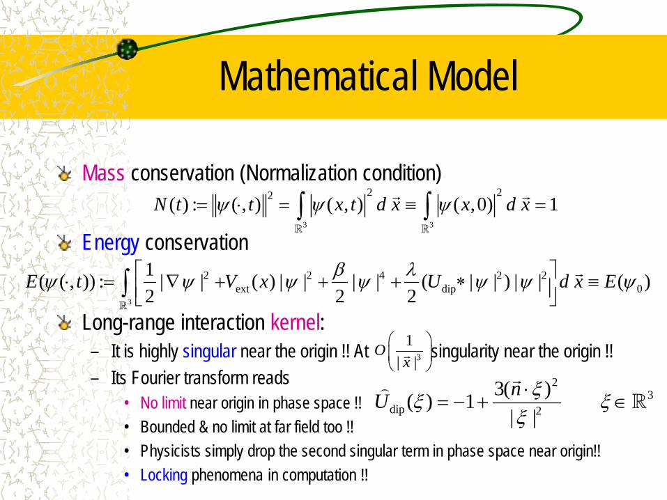
Mass conservation (Normalization condition) Energy conservation

Long-range interaction kernel: – It is highly singular near the origin !! At singularity near the origin !! – Its Fourier transform reads

• No limit near origin in phase space !! • Bounded & no limit at far field too !! • Physicists simply drop the second singular term in phase space near origin!! • Locking phenomena in computation !!

3 3

2 22( ) : ( , ) ( , ) ( ,0) 1N t t x t d x x d xψ ψ ψ= ⋅ = ≡ =∫ ∫

3

2 2 4 2 2ext dip 0

1( ( , )) : | | ( ) | | | | ( | | ) | | ( )2 2 2

E t V x U d x Eβ λψ ψ ψ ψ ψ ψ ψ ⋅ = ∇ + + + ∗ ≡ ∫

23

dip 23( )( ) 1

| |nU ξξ ξξ⋅

= − + ∈

31

| |O

x

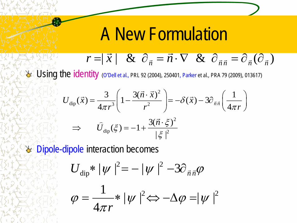
A New Formulation

Using the identity (O’Dell et al., PRL 92 (2004), 250401, Parker et al., PRA 79 (2009), 013617)

Dipole-dipole interaction becomes

2

dip 3 2

2

dip 2

3 3( ) 1( ) 1 ( ) 3 4 4

3( ) ( ) 1| |

n nn xU x x

r r r

nU

δπ π

ξξξ

⋅ = − = − − ∂

⋅⇒ = − +

2 2dip

2 2

| | | | 3

1 | | | |4

n nU

r

ψ ψ ϕ

ϕ ψ ϕ ψπ

∗ = − − ∂

= ∗ ⇔ −∆ =

| | & & ( )n n n n nr x n= ∂ = ⋅∇ ∂ = ∂ ∂

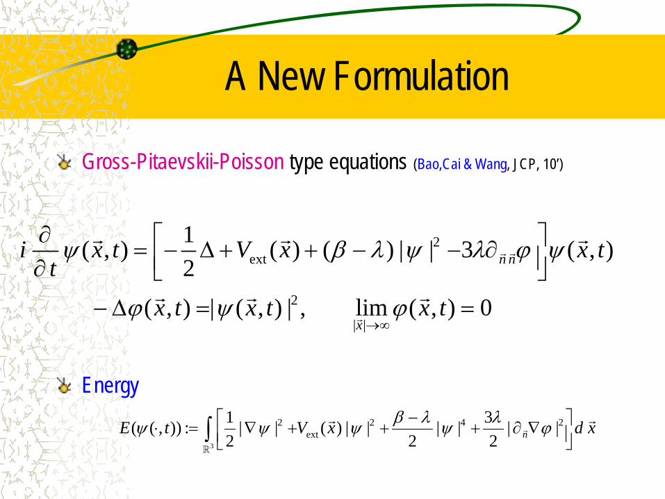
A New Formulation

Gross-Pitaevskii-Poisson type equations (Bao,Cai & Wang, JCP, 10’)

Energy

2ext

2

| |

1( , ) ( ) ( ) | | 3 ( , )2

( , ) | ( , ) | , lim ( , ) 0

n n

x

i x t V x x tt

x t x t x t

ψ β λ ψ λ ϕ ψ

ϕ ψ ϕ→∞

∂ = − ∆ + + − − ∂ ∂ − ∆ = =

3

2 2 4 2ext

1 3( ( , )) : | | ( ) | | | | | |2 2 2 nE t V x d xβ λ λψ ψ ψ ψ ϕ− ⋅ = ∇ + + + ∂ ∇ ∫

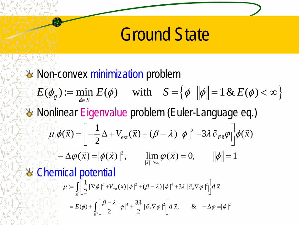
Ground State

Non-convex minimization problem

Nonlinear Eigenvalue problem (Euler-Language eq.)

Chemical potential

2ext

2

| |

1( ) ( ) ( ) | | 3 ( )2

( ) | ( ) | , lim ( ) 0, 1

n n

x

x V x x

x x x

µ φ β λ φ λ ϕ φ

ϕ φ ϕ φ→∞

= − ∆ + + − − ∂ − ∆ = = =

( ) : min ( ) with | 1& ( )g SE E S E

φφ φ φ φ φ

∈= = = < ∞

3

3

2 2 4 2ext

4 2 2

1: | | ( ) | | ( ) | | 3 | |2

3( ) | | | | , & | |2 2

n

n

V x d x

E d x

µ φ φ β λ φ λ ϕ

β λ λφ φ ϕ ϕ φ

= ∇ + + − + ∂ ∇

− = + + ∂ ∇ − ∆ =

∫

∫

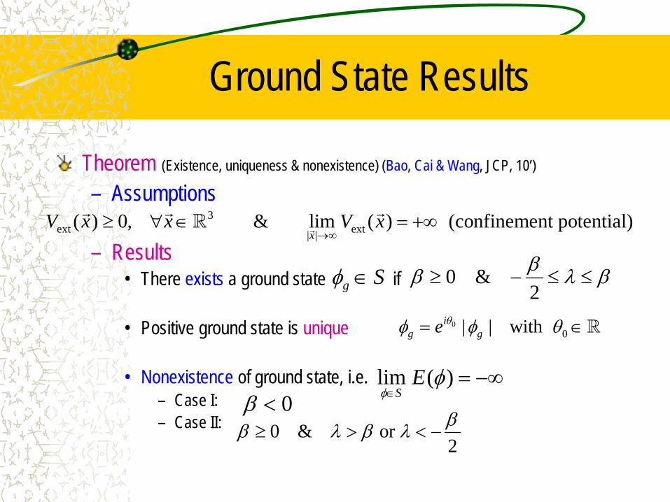
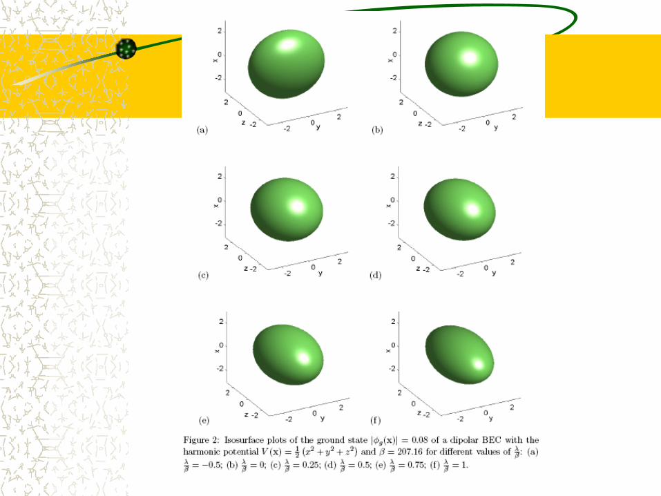
Ground State Results

Theorem (Existence, uniqueness & nonexistence) (Bao, Cai & Wang, JCP, 10’) – Assumptions

– Results

• There exists a ground state if • Positive ground state is unique • Nonexistence of ground state, i.e.

– Case I: – Case II:

3ext ext| |

( ) 0, & lim ( ) (confinement potential)x

V x x V x→∞

≥ ∀ ∈ = +∞

g Sφ ∈ 0 &2ββ λ β≥ − ≤ ≤

00| | with i

g ge θφ φ θ= ∈

lim ( )S

Eφ

φ∈

= −∞0β <

0 & or 2ββ λ β λ≥ > < −

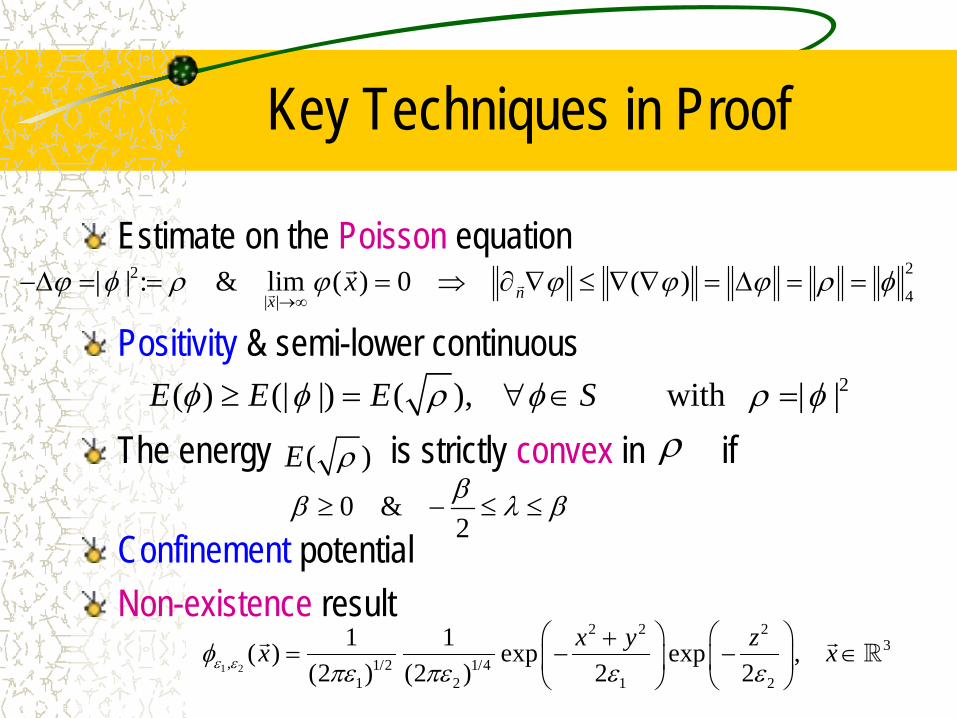
Key Techniques in Proof

Estimate on the Poisson equation Positivity & semi-lower continuous The energy is strictly convex in if Confinement potential Non-existence result

2( ) (| |) ( ), with | |E E E Sφ φ ρ φ ρ φ≥ = ∀ ∈ =

224| |

| | : & lim ( ) 0 ( )nxxϕ φ ρ ϕ ϕ ϕ ϕ ρ φ

→∞−∆ = = = ⇒ ∂ ∇ ≤ ∇ ∇ = ∆ = =

( )E ρ ρ0 &

2ββ λ β≥ − ≤ ≤

1 2

2 2 23

, 1/2 1/41 2 1 2

1 1( ) exp exp ,(2 ) (2 ) 2 2

x y zx xε εφπε πε ε ε

+= − − ∈

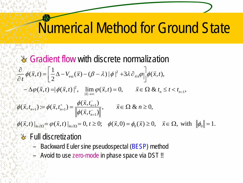
Numerical Method for Ground State

Gradient flow with discrete normalization Full discretization – Backward Euler sine pseudospectal (BESP) method – Avoid to use zero-mode in phase space via DST !!

2ext

21| |

11 1

1

1( , ) ( ) ( ) | | 3 ( , ),2

( , ) | ( , ) | , lim ( , ) 0, & ,

( , )( , ) : ( , ) , & 0,( , )

( , ) | ( , ) | 0, 0

n n

n nx

nn n

n

x x

x t V x x tt

x t x t x t x t t t

x tx t x t x nx t

x t x t t

φ β λ φ λ ϕ φ

ϕ φ ϕ

φφ φφ

φ ϕ

+→∞

−+ +

+ + −+

∈∂Ω ∈∂Ω

∂ = ∆ − − − + ∂ ∂ − ∆ = = ∈Ω ≤ <

= = ∈Ω ≥

= = ≥

0 0; ( ,0) ( ) 0, , with 1.x x xφ φ φ= ≥ ∈Ω =

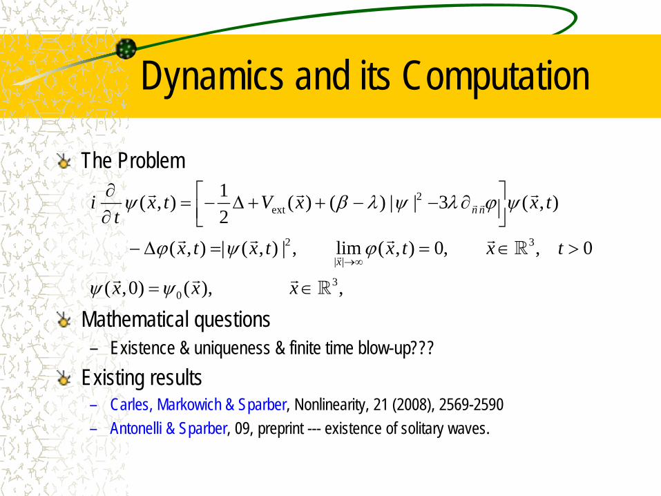
Dynamics and its Computation

The Problem

Mathematical questions – Existence & uniqueness & finite time blow-up???

Existing results – Carles, Markowich & Sparber, Nonlinearity, 21 (2008), 2569-2590 – Antonelli & Sparber, 09, preprint --- existence of solitary waves.

2ext

2 3

| |

30

1( , ) ( ) ( ) | | 3 ( , )2

( , ) | ( , ) | , lim ( , ) 0, , 0

( ,0) ( ), ,

n n

x

i x t V x x tt

x t x t x t x t

x x x

ψ β λ ψ λ ϕ ψ

ϕ ψ ϕ

ψ ψ→∞

∂ = − ∆ + + − − ∂ ∂ − ∆ = = ∈ >

= ∈

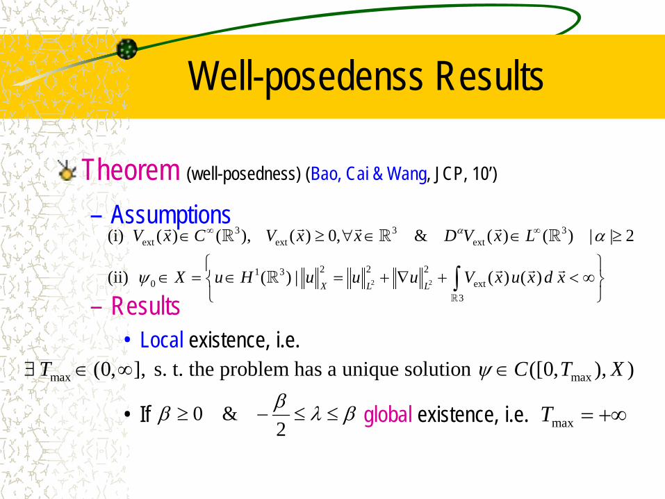
Well-posedenss Results

Theorem (well-posedness) (Bao, Cai & Wang, JCP, 10’) – Assumptions

– Results

• Local existence, i.e.

• If global existence, i.e.

2 2

3 3 3ext ext ext

2 2 21 30 ext

3

(i) ( ) ( ), ( ) 0, & ( ) ( ) | | 2

(ii) ( ) | ( ) ( )X L L

V x C V x x D V x L

X u H u u u V x u x d x

α α

ψ

∞ ∞∈ ≥ ∀ ∈ ∈ ≥

∈ = ∈ = + ∇ + < ∞

∫

0 &2ββ λ β≥ − ≤ ≤

max max(0, ], s. t. the problem has a unique solution ([0, ), )T C T Xψ∃ ∈ ∞ ∈

maxT = +∞

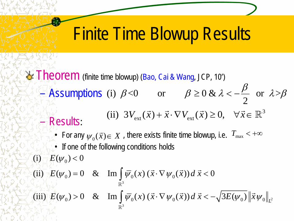
Finite Time Blowup Results

Theorem (finite time blowup) (Bao, Cai & Wang, JCP, 10’) – Assumptions

– Results: • For any , there exists finite time blowup, i.e. • If one of the following conditions holds

3ext ext

(i) <0 or 0 & or >2

(ii) 3 ( ) ( ) 0,V x x V x x

ββ β λ λ β≥ < −

+ ⋅∇ ≥ ∀ ∈

maxT < +∞0( )x Xψ ∈

3

2

3

0

0 0 0

0 0 0 0 0

(i) ( ) 0

(ii) ( ) 0 & Im ( ) ( ( )) 0

(iii) ( ) 0 & Im ( ) ( ( )) 3 ( )L

E

E x x x d x

E x x x d x E x

ψ

ψ ψ ψ

ψ ψ ψ ψ ψ

<

= ⋅∇ <

> ⋅∇ < −

∫

∫

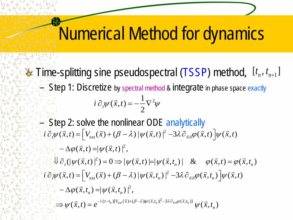
Numerical Method for dynamics

Time-splitting sine pseudospectral (TSSP) method, – Step 1: Discretize by spectral method & integrate in phase space exactly

– Step 2: solve the nonlinear ODE analytically

1[ , ]n nt t +

21( , )2ti x tψ ψ∂ = − ∇

2ext

2

2

2ext

( , ) ( ) ( ) | ( , ) | 3 ( , ) ( , )

( , ) | ( , ) | , (| ( , ) | ) 0 | ( , ) | | ( , ) | & ( , ) ( , )

( , ) ( ) ( ) | ( , ) | 3 ( , ) (

t n n

t n n

t n n n n

i x t V x x t x t x t

x t x tx t x t x t x t x t

i x t V x x t x t

ψ β λ ψ λ ϕ ψ

ϕ ψ

ψ ψ ψ ϕ ϕ

ψ β λ ψ λ ϕ ψ

∂ = + − − ∂ − ∆ =

⇓ ∂ = ⇒ = =

∂ = + − − ∂

2ext

2

( )[ ( ) ( )| ( , )| 3 ( , )]

, )

( , ) | ( , ) | ,

( , ) ( , )n n n n n

n n

i t t V x x t x tn

x t

x t x t

x t e x tβ λ ψ λ ϕ

ϕ ψ

ψ ψ− − + − − ∂

− ∆ =

⇒ =

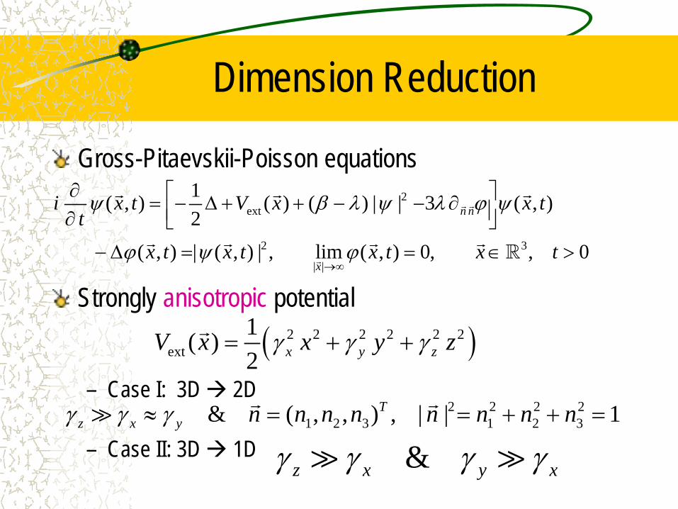
Dimension Reduction

Gross-Pitaevskii-Poisson equations Strongly anisotropic potential

– Case I: 3D 2D – Case II: 3D 1D

( )2 2 2 2 2 2ext

1( )2 x y zV x x y zγ γ γ= + +

2 2 2 21 2 3 1 2 3& ( , , ) , | | 1T

z x y n n n n n n n nγ γ γ≈ = = + + =

&z x y xγ γ γ γ

2ext

2 3

| |

1( , ) ( ) ( ) | | 3 ( , )2

( , ) | ( , ) | , lim ( , ) 0, , 0

n n

x

i x t V x x tt

x t x t x t x t

ψ β λ ψ λ ϕ ψ

ϕ ψ ϕ→∞

∂ = − ∆ + + − − ∂ ∂ − ∆ = = ∈ >

Dimension Reduction

Existing results – BEC without dipole-dipole interaction:

• Formal asymptotic (Bao, Markowich, Schmeiser & Weishaupl, M3AS, 05’)

• Numerical results (Bao, Ge, Jaksch, Markowich & Weishaeupl, CPC, 07’)

• Rigorous proof (Ben Abdallah, Mehats et al., SIMA, 05; JDE 08’)

• From N-body to mean field theory (Lieb, Seiringer & Yngvason, CMP, 04’; Erdos, Schlein & Yau, Ann. Math., 10’)

– Dipolar BEC (Carles, Markowich & Sparber, Nonlinearity, 08’) – formal result

0λ =

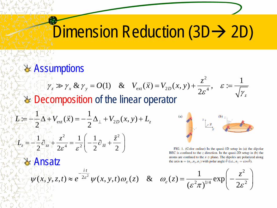
Dimension Reduction (3D 2D)

Assumptions

Decomposition of the linear operator Ansatz

2

ext 2 4

1& (1) & ( ) ( , ) , :2z x y D

z

zO V x V x yγ γ γ εε γ

= = + =

22

22 1/4 21( , , , ) ( , , ) ( ) & ( ) exp

( ) 2

i t zx y z t e x y t z zεε εψ ψ ω ω

ε π ε−

≈ = −

2 2

4 2

1 1 12 2 2 2z zz zz

z zLε ε

= − ∂ + = − ∂ +

ext 21 1: ( ) ( , )2 2 D zL V x V x y L⊥= − ∆ + = − ∆ + +

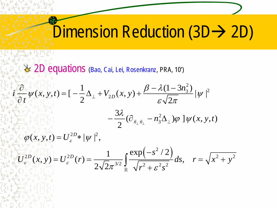
Dimension Reduction (3D 2D)

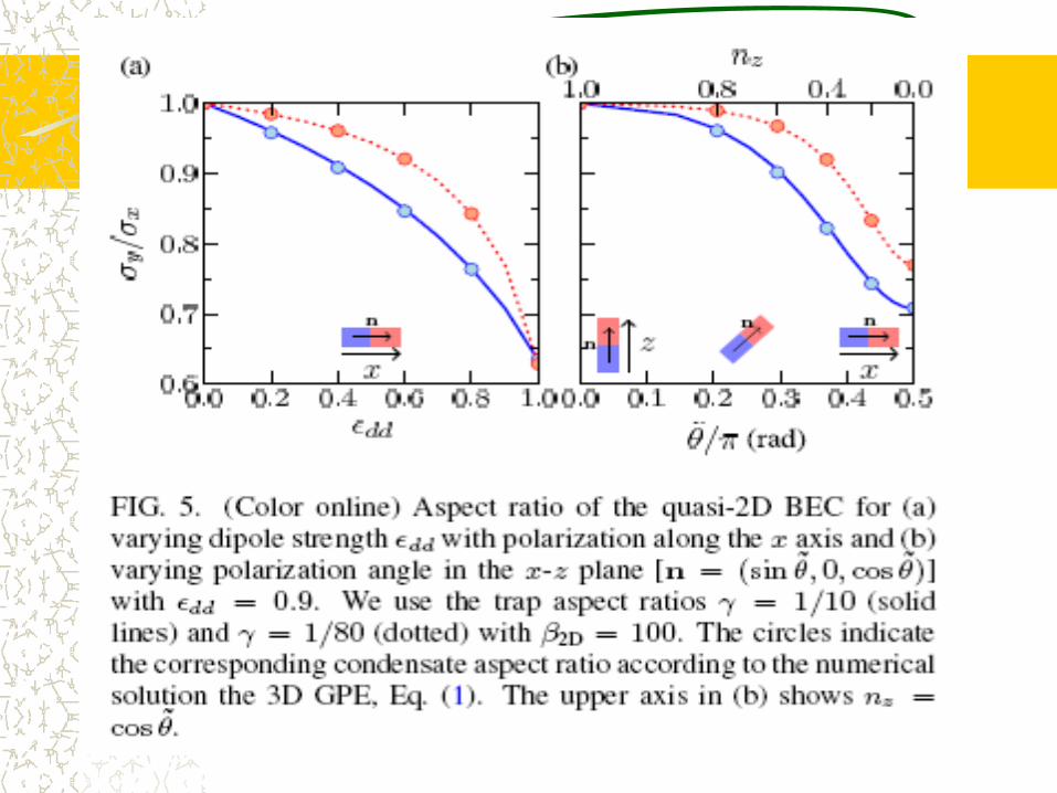
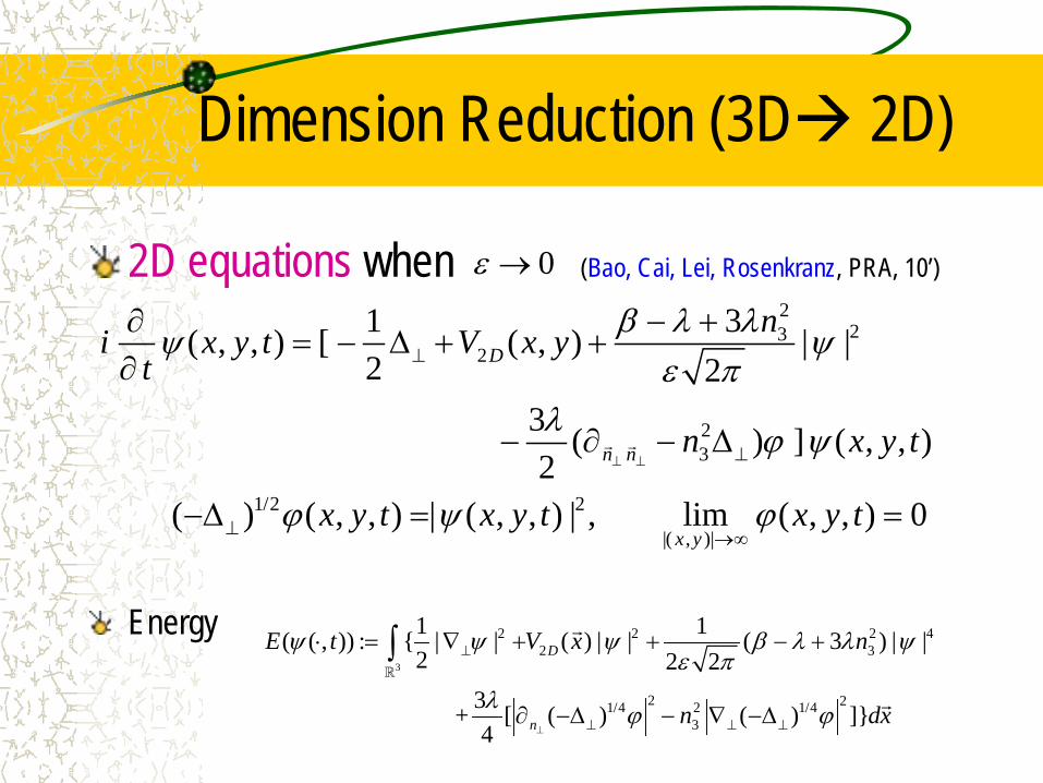
2D equations (Bao, Cai, Lei, Rosenkranz, PRA, 10’)

( )

223

2

23

2 2

22 2 2 2

3/2 2 2 2

1 (1 3 )( , , ) [ ( , ) | |2 2

3 ( ) ] ( , , )2

( , , ) | | ,

exp / 21 ( , ) ( ) , 2 2

D

n n

D

D D

ni x y t V x yt

n x y t

x y t U

sU x y U r ds r x y

r s

ε

ε ε

β λψ ψε π

λ ϕ ψ

ϕ ψ

π ε

⊥ ⊥

⊥

⊥

∂ − −= − ∆ + +

∂

− ∂ − ∆

= ∗

−= = = +

+∫

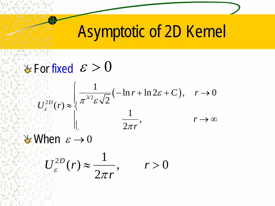
Asymptotic of 2D Kernel

For fixed When

0ε >( )3/2

2

1 ln ln 2 , 02( )

1 ,2

Dr C r

U rr

r

ε

επ ε

π

− + + →≈ → ∞

0ε →

2 1( ) , 02

DU r rrε π

≈ >

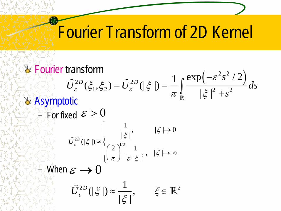
Fourier Transform of 2D Kernel

Fourier transform Asymptotic – For fixed

– When

21/2

2

1 , | | 0| |

(| |)2 1 , | |

| |

DUε

ξξ

ξξ

π ε ξ

→≈ → ∞

( )2 22 2

1 2 2 2

exp / 21( , ) (| |)| |

D D sU U ds

sε ε

εξ ξ ξ

π ξ−

= =+∫

0ε >

0ε →2 21(| |) ,

| |DUε ξ ξ

ξ≈ ∈

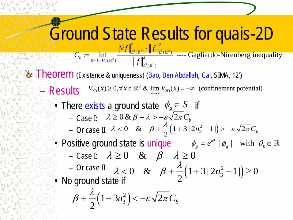
Ground State Results for quais-2D

Theorem (Existence & uniqueness) (Bao, Ben Abdallah, Cai, SIMA, 12’) – Results

• There exists a ground state if – Case I: – Or case II

• Positive ground state is unique – Case I: – Or case II

• No ground state if

0 & 0λ β λ≥ − ≥

22D 2D| |

( ) 0, & lim ( ) (confinement potential)x

V x x V x→∞

≥ ∀ ∈ = +∞

g Sφ ∈

( )230 & 1 3 | 2 1 | 2

2 bn Cλλ β ε π< + + − > −

00| | with i

g ge θφ φ θ= ∈

0 & 2 bCλ β λ ε π≥ − > −

( )230 & 1 3 | 2 1 | 0

2nλλ β< + + − ≥

2 2 2 2

1 24 2

2 2

( ) ( )40 ( )

( )

: inf ---- Gagliardo-Nirenberg inequalityL Lb f H

L

f fC

f≠ ∈

∇ ⋅=

( )231 3 2

2 bn Cλβ ε π+ − < −

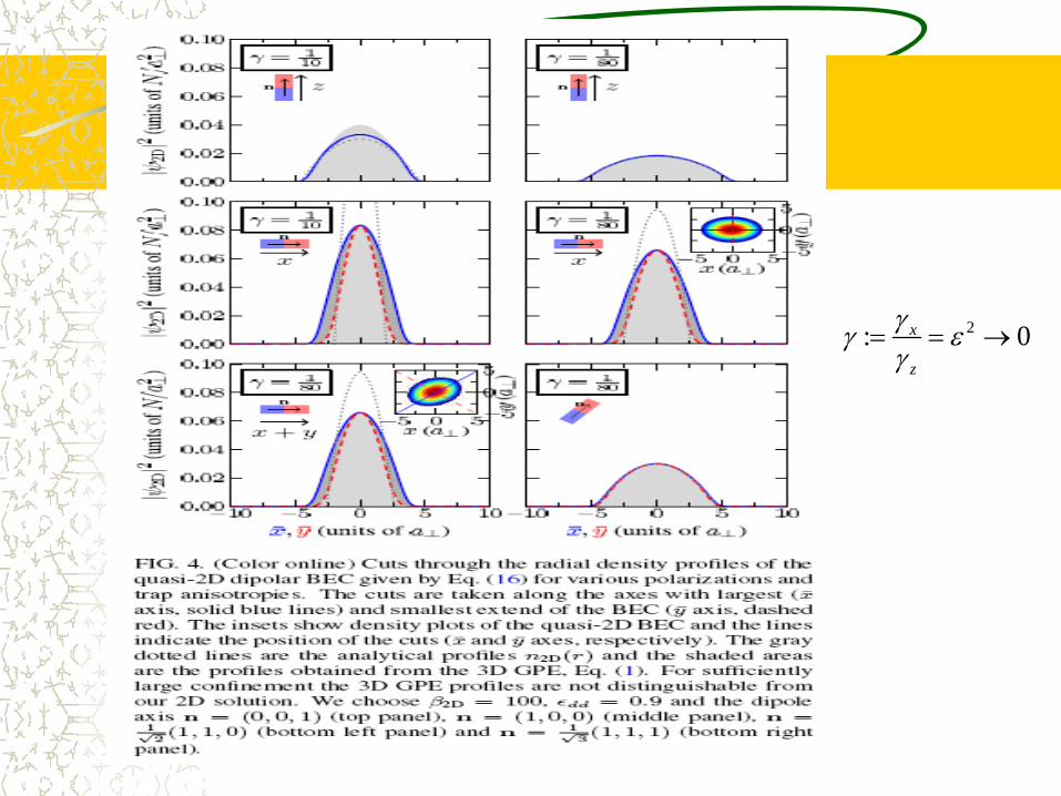
2: 0x

z

γγ εγ

= = →

Dimension Reduction (3D 2D)

2D equations when (Bao, Cai, Lei, Rosenkranz, PRA, 10’)

Energy

223

2

23

1/2 2

|( , )|

1 3( , , ) [ ( , ) | |2 2

3 ( ) ] ( , , )2

( ) ( , , ) | ( , , ) | , lim ( , , ) 0

D

n n

x y

ni x y t V x yt

n x y t

x y t x y t x y t

β λ λψ ψε π

λ ϕ ψ

ϕ ψ ϕ

⊥ ⊥

⊥

⊥

⊥ →∞

∂ − += − ∆ + +

∂

− ∂ − ∆

−∆ = =

0ε →

3

2 2 2 42 3

2 21/4 2 1/43

1 1( ( , )) : | | ( ) | | ( 3 ) | |2 2 2

3 + [ ( ) ( ) ]4

D

n

E t V x n

n dx

ψ ψ ψ β λ λ ψε π

λ ϕ ϕ⊥

⊥

⊥ ⊥ ⊥

⋅ = ∇ + + − +

∂ −∆ − ∇ −∆

∫

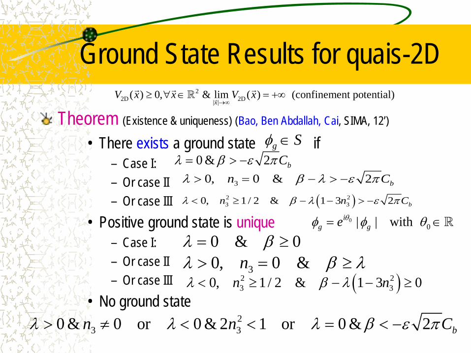
Ground State Results for quais-2D

Theorem (Existence & uniqueness) (Bao, Ben Abdallah, Cai, SIMA, 12’) • There exists a ground state if

– Case I: – Or case II – Or case III

• Positive ground state is unique – Case I: – Or case II – Or case III

• No ground state

0 & 0λ β= ≥

22D 2D| |

( ) 0, & lim ( ) (confinement potential)x

V x x V x→∞

≥ ∀ ∈ = +∞

g Sφ ∈

30, 0 & 2 bn Cλ β λ ε π> = − > −

00| | with i

g ge θφ φ θ= ∈

0 & 2 bCλ β ε π= > −

30, 0 &nλ β λ> = ≥

( )2 23 30, 1 / 2 & 1 3 2 bn n Cλ β λ ε π< ≥ − − > −

( )2 23 30, 1 / 2 & 1 3 0n nλ β λ< ≥ − − ≥

23 30 & 0 or 0 & 2 1 or 0 & 2 bn n Cλ λ λ β ε π> ≠ < < = < −

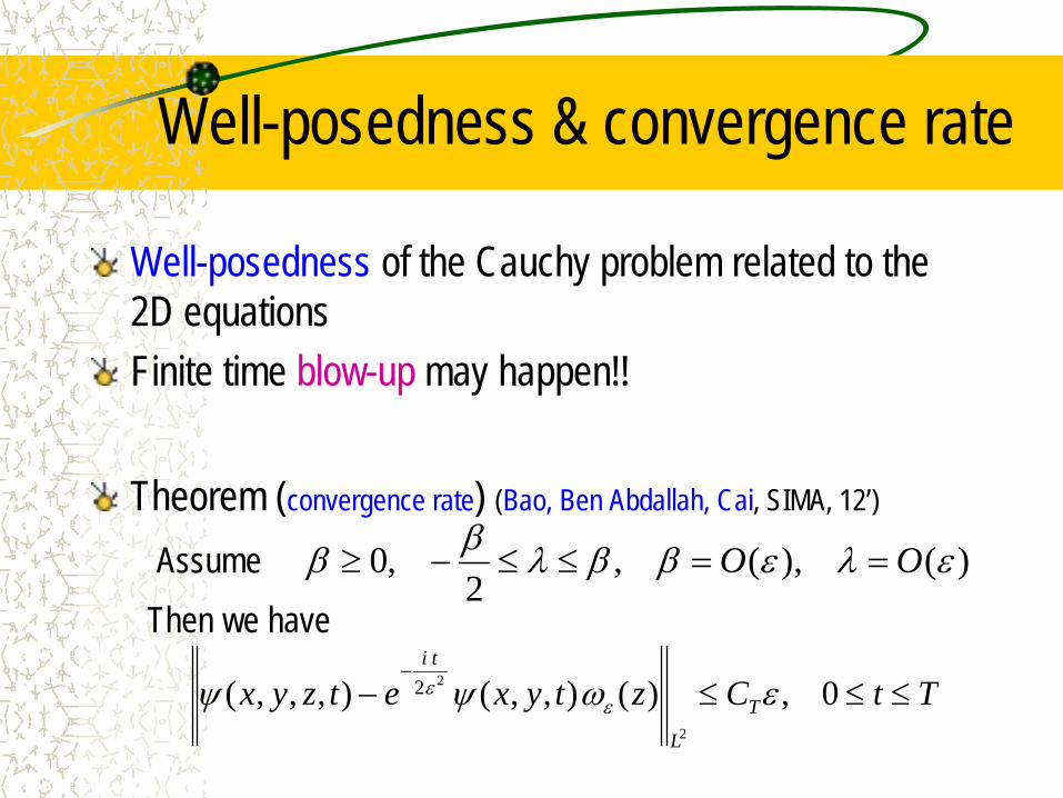
Well-posedness & convergence rate

Well-posedness of the Cauchy problem related to the 2D equations Finite time blow-up may happen!!

Theorem (convergence rate) (Bao, Ben Abdallah, Cai, SIMA, 12’) Assume Then we have

0, , ( ), ( )2

O Oββ λ β β ε λ ε≥ − ≤ ≤ = =

2

2

2( , , , ) ( , , ) ( ) , 0i t

T

L

x y z t e x y t z C t Tεεψ ψ ω ε

−− ≤ ≤ ≤

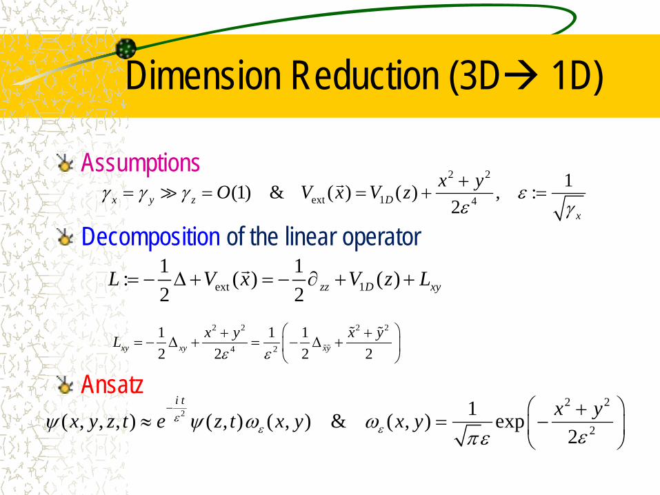
Dimension Reduction (3D 1D)

Assumptions Decomposition of the linear operator Ansatz

2 2

ext 1 4

1(1) & ( ) ( ) , :2x y z D

x

x yO V x V zγ γ γ εε γ+

= = = + =

22 2

21( , , , ) ( , ) ( , ) & ( , ) exp

2

i t x yx y z t e z t x y x yεε εψ ψ ω ω

επε

− +≈ = −

2 2 2 2

4 2

1 1 12 2 2 2xy xy xy

x y x yLε ε

+ += − ∆ + = − ∆ +

ext 11 1: ( ) ( )2 2 zz D xyL V x V z L= − ∆ + = − ∂ + +

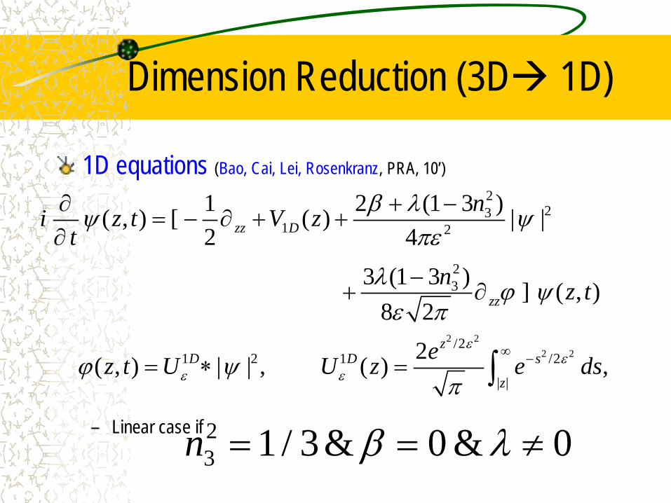
Dimension Reduction (3D 1D)

1D equations (Bao, Cai, Lei, Rosenkranz, PRA, 10’)

– Linear case if

2 22 2

223

1 2

23

/21 2 1 /2

| |

1 2 (1 3 )( , ) [ ( ) | |2 4

3 (1 3 ) ] ( , )8 2

2 ( , ) | | , ( ) ,

zz D

zz

zD D s

z

ni z t V zt

n z t

ez t U U z e dsε

εε ε

β λψ ψπε

λ ϕ ψε π

ϕ ψπ

∞ −

∂ + −= − ∂ + +

∂

−+ ∂

= ∗ = ∫23 1 / 3& 0 & 0n β λ= = ≠

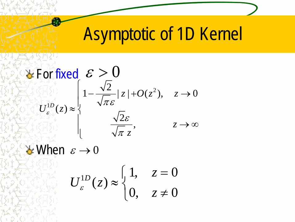
Asymptotic of 1D Kernel

For fixed When

0ε >2

1

21 | | ( ), 0( )

2 ,

D

z O z zU z

zz

επ ε

επ

− + →

≈ → ∞

0ε →

1 1, 0( )

0, 0D z

U zzε

=≈ ≠

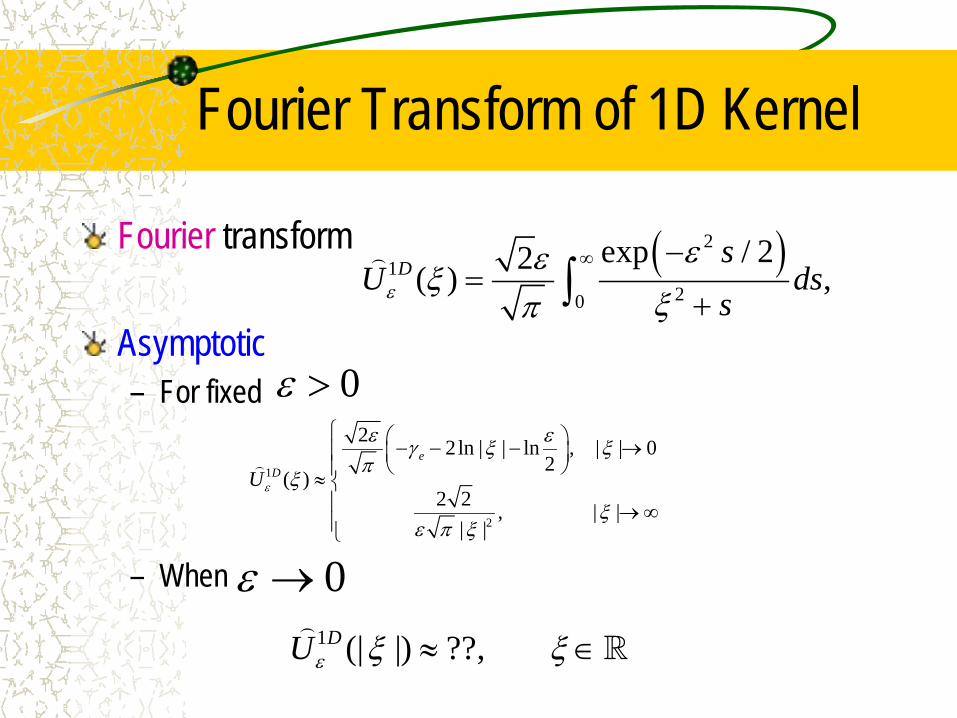
Fourier Transform of 1D Kernel

Fourier transform Asymptotic – For fixed

– When

1

2

2 2 ln | | ln , | | 02

( )2 2 , | |

| |

eDUε

ε εγ ξ ξπ

ξξ

ε π ξ

− − − → ≈

→ ∞

( )21

20

exp / 22( ) ,D sU ds

sε

εεξξπ

∞ −=

+∫

0ε >

0ε →1 (| |) ??,DUε ξ ξ≈ ∈

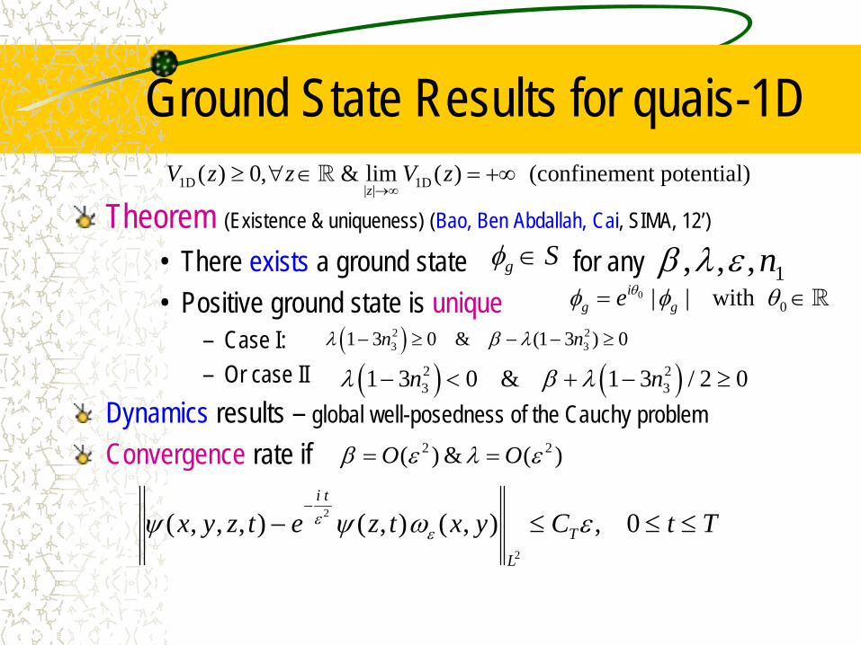
Ground State Results for quais-1D

Theorem (Existence & uniqueness) (Bao, Ben Abdallah, Cai, SIMA, 12’) • There exists a ground state for any • Positive ground state is unique

– Case I: – Or case II

Dynamics results – global well-posedness of the Cauchy problem Convergence rate if

( )2 23 31 3 0 & (1 3 ) 0n nλ β λ− ≥ − − ≥

1D 1D| |( ) 0, & lim ( ) (confinement potential)

zV z z V z

→∞≥ ∀ ∈ = +∞

g Sφ ∈0

0| | with ig ge θφ φ θ= ∈

( ) ( )2 23 31 3 0 & 1 3 / 2 0n nλ β λ− < + − ≥

1, , ,nβ λ ε

2 2( ) & ( )O Oβ ε λ ε= =

2

2

( , , , ) ( , ) ( , ) , 0i t

T

L

x y z t e z t x y C t Tεεψ ψ ω ε

−− ≤ ≤ ≤

2

1: x

z

γγγ ε

= = → ∞

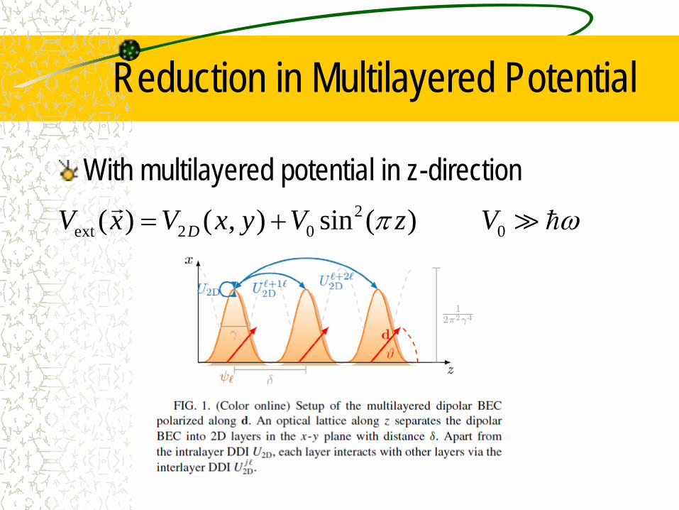
Reduction in Multilayered Potential

With multilayered potential in z-direction 2

ext 2 0 0( ) ( , ) sin ( ) DV x V x y V z Vπ ω= +

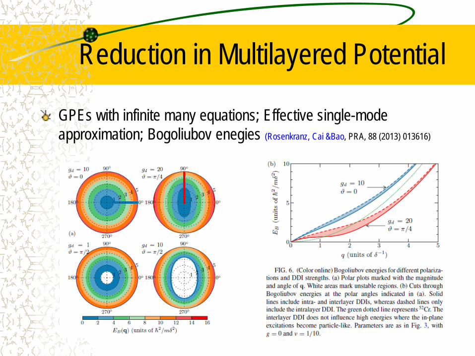
Reduction in Multilayered Potential

GPEs with infinite many equations; Effective single-mode approximation; Bogoliubov enegies (Rosenkranz, Cai &Bao, PRA, 88 (2013) 013616)

Conclusion & future challenges

Conclusion – Ground state in 3D – existence, uniqueness & nonexistence

– Dynamics in 3D – well-posedness & finite time blowup – Efficient numerical methods via DST – Dimension Reduction --- 3D 2D & 3D1D – Ground states and dynamics in quasi-2D & quasi-1D

Future challenges – Convergence rate for reduction in O(1) regime – In rotating frame & multi-component & spin-1 – Dipolar BEC with random potential – disorder!!