
MODELING AIRCRAFT FUEL CONSUMPTION WITH A NEURAL … · MATLAB and its accompanying Neural Network...
123
MODELING AIRCRAFT FUEL CONSUMPTION WITH A NEURAL NETWORK by Glenn D. Schilling Thesis submitted to the faculty of the Virginia Polytechnic Institute and State University in partial fulfillment of the requirements for the degree of MASTER OF SCIENCE IN CIVIL ENGINEERING APPROVED: Antonio A. Trani, Ph.D., Chairman Donald R. Drew, Ph.D. Richard G. Greene, Ph.D. February, 1997 Blacksburg, Virginia Keywords: Aviation, Aircraft Performance, Backpropagation, Models
Transcript of MODELING AIRCRAFT FUEL CONSUMPTION WITH A NEURAL … · MATLAB and its accompanying Neural Network...
MODELING AIRCRAFT FUEL CONSUMPTION
WITH A NEURAL NETWORK
by
Glenn D. Schilling
Thesis submitted to the faculty of the
Virginia Polytechnic Institute and State University
in partial fulfillment of the requirements for the degree of
MASTER OF SCIENCE
IN
CIVIL ENGINEERING
APPROVED:
Antonio A. Trani, Ph.D., Chairman
Donald R. Drew, Ph.D. Richard G. Greene, Ph.D.
February, 1997
Blacksburg, Virginia
Keywords: Aviation, Aircraft Performance, Backpropagation, Models

MODELING AIRCRAFT FUEL CONSUMPTION
WITH A NEURAL NETWORK
by
Glenn D. Schilling
Dr. A. A. Trani, Chairman
Civil Engineering
(ABSTRACT)
This research involves the development of an aircraft fuel consumption model to
simplify Bela Collins of the MITRE Corporation aircraft fuelburn model in terms of level
of computation and level of capability. MATLAB and its accompanying Neural Network
Toolbox, has been applied to data from the base model to predict fuel consumption. The
approach to the base model and neural network is detailed in this paper. It derives from
the basic concepts of energy balance. Multivariate curve fitting techniques used in
conjunction with aircraft performance data derive the aircraft specific constants. Aircraft
performance limits are represented by empirical relationships that also utilize aircraft
specific constants. It is based on generally known assumptions and approximations for
commercial jet operations. It will simulate fuel consumption by adaptation of a specific
aircraft using constants that represent the relationship of lift-to-drag and thrust-to-fuel
flow.
The neural network model invokes the output from MITRE’s algorithm and
provides: (1) a comparison to the polynomial fuelburn function in the fuelburn post-
processor of the FAA Airport and Airspace Simulation Model (SIMMOD), (2) an
established sensitivity of system performance for a range of variables that effect fuel
consumption, (3) a comparison of post fuel burn (fuel consumption algorithms)
techniques to new techniques, and (4) the development of a trained demo neural network.
With the powerful features of optimization, graphics, and hierarchical modeling,
the MATLAB toolboxes proved to be effective in this modeling process.

Acknowledgments iii
ACKNOWLEDGMENTS
I sincerely wish to express my gratitude to my advisor Dr. Antonio Trani for his
full support, expert guidance, understanding and encouragement throughout the course of
this research. Also, I am greatly indebted to him for his critical review of the manuscript
of my thesis.
I would like to thank my committee members, Dr. Donald Drew and Dr. Richard
Greene, for serving on my committee, and providing me with excellent course instruction
during my graduate years at Virginia Tech.
It is my greatest pleasure to dedicate this thesis to my parents, my dream was
accomplished by their help. I would also like to thank my brother’s and sister’s-in-law for
their unconditional support throughout my entire collegiate career.
Finally, I would like to thank the many friends who encouraged me to continue
my higher education at Virginia Tech.

Table of Contents iv
TABLE of CONTENTS
Chapter Page
1. Introduction
1.1 Purpose.......................................................................................................... 1
1.2 Background ................................................................................................... 1
1.3 Fuel Consumption Modeling ........................................................................ 2
1.4 Fuelburn Background.................................................................................... 3
1.5 Research Approach, and Objective............................................................... 5
2. Literature Review
2.1 Introduction .................................................................................................. 7
2.2 Aerodynamic Forces ..................................................................................... 7
2.2.1 Temperature ......................................................................................... 9
2.2.2 Pressure ................................................................................................ 9
2.2.3 Density ................................................................................................. 10
2.2.4 Viscosity............................................................................................... 12
2.2.5 Sonic Velocity...................................................................................... 12
2.3 Performance Characteristics of Aircraft........................................................ 15
2.4 Advanced Fuelburn Model Assumptions...................................................... 17
2.5 Advanced Fuelburn Model (AFBM)............................................................. 18
2.6 The Power of Neural Networks..................................................................... 22
2.6.1 Elements of the Neural Network Paradigm.......................................... 23
2.6.2 Network Architecture........................................................................... 26
2.6.3 Transfer Functions ............................................................................... 27
2.6.4 Backpropagation .................................................................................. 29
2.6.5 Levenberg-Marquardt Backpropagation Algorithm............................. 31
Table of Contents v
Chapter Page
3. Methodology
3.1 Introduction................................................................................................... 42
3.2 Models and Nonlinear Optimization............................................................. 42
3.3 Approach to Model Development................................................................. 44
3.4 Aircraft Fuel Consumption Model Assumptions .......................................... 46
3.5 Description of MATLAB.............................................................................. 47
3.6 Research Discussion and Pertaining Questions ............................................ 48
4. Model Description
4.1 Introduction................................................................................................... 54
4.2 Specifics of the Neural Network................................................................... 54
4.3 Statistics of Performance Data...................................................................... 60
4.3.1 Statistical Methods............................................................................... 60
4.4 Output of the Model ...................................................................................... 64
5. Model Application and Analysis
5.1 Introduction................................................................................................... 65
5.2 Model Application ........................................................................................ 65
5.3 Model Input Parameters ................................................................................ 66
5.4 Model Results ............................................................................................... 69
5.4.1 Graphical Analysis ............................................................................... 69
5.4.2 Statistical Analysis ............................................................................... 79
5.5 Statistical Results .......................................................................................... 86
6. Conclusions and Recommendations
6.1 Introduction................................................................................................... 87
6.2 Conclusions................................................................................................... 87
6.3 Recommendations......................................................................................... 89
Bibliography .................................................................................................................. 91

Table of Contents vi
Appendix A. Aircraft Specific Constants .................................................................. 95
B. AFCM Program..................................................................................... 100
C. MINITAB Session Worksheets ........................................................... 107
D. Weight and Bias Matrix Output of AFCM......................................... 110
List of Figures vii
LIST of FIGURES
Figure Page
1. Flight Path Free Body Diagram........................................................................... 8
2. Layer of S Neurons with R Inputs....................................................................... 25
3. Two-Layer Tansig/Purelin Network ................................................................... 26
4. Tan-Sigmoid Transfer Function.......................................................................... 28
5. BP Learning Schematics ..................................................................................... 30
6. Three-Layer Neural Network.............................................................................. 51
7. Two Dimensional Input Vector........................................................................... 55
8. Partial Aircraft Echo Report................................................................................ 67
9. Velocity and Altitude Profiles............................................................................. 72
10. Fuel Consumption Before Network Training...................................................... 73
11. Lift and Drag Relationships vs. Mach Number................................................... 74
12. Mach Functions vs. Mach Number ..................................................................... 75
13. Trained vs. Actual Fuel Consumption and Generalized vs. Trained
Fuel Consumption ............................................................................................... 76
14. Comparison of Fuel Consumption Data.............................................................. 77
15. Comparison of Specific Input Fuel Consumption Data ...................................... 78
16. Summary of AFBM-NNOM Statistical Results.................................................. 79
17. Fuel Consumption Differences of a Boeing 747-100.......................................... 80
18. Fuel Consumption Differences of a Boeing 767-200.......................................... 82
19. Fuel Consumption Differences of a Bombardier Dash-7.................................... 83
20. Fuel Consumption Differences of a McDonnel-DouglasDC10-30..................... 84
21. Fuel Consumption Differences of a Lockheed Martin Jetstar............................. 85
22. Summary of Statistical Results ........................................................................... 86

List of Tables viii
LIST of TABLES
Table Page
1. U.S. Standard Atmosphere.................................................................................. 14
2. Floating Point Operations ................................................................................... 68
1. Introduction 1
1. INTRODUCTION
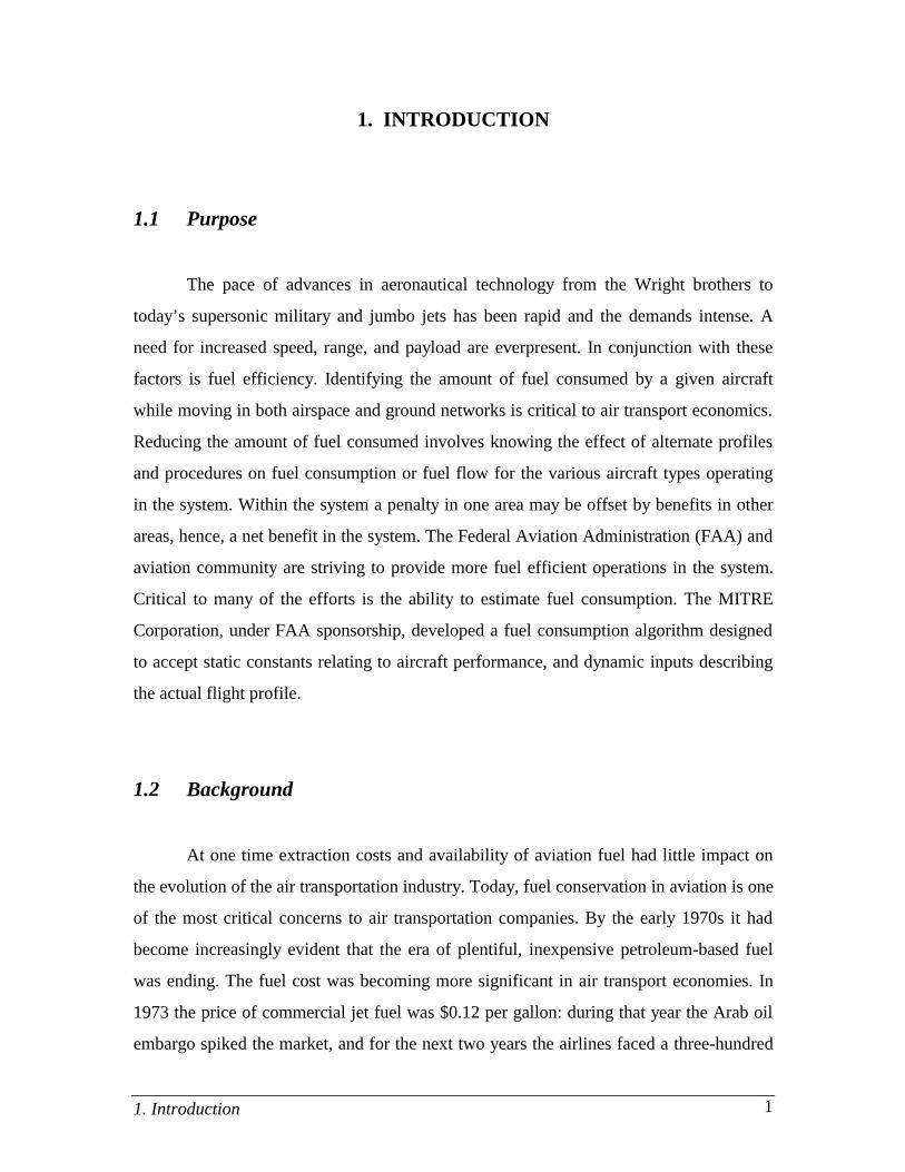
1.1 Purpose
The pace of advances in aeronautical technology from the Wright brothers to
today’s supersonic military and jumbo jets has been rapid and the demands intense. A
need for increased speed, range, and payload are everpresent. In conjunction with these
factors is fuel efficiency. Identifying the amount of fuel consumed by a given aircraft
while moving in both airspace and ground networks is critical to air transport economics.
Reducing the amount of fuel consumed involves knowing the effect of alternate profiles
and procedures on fuel consumption or fuel flow for the various aircraft types operating
in the system. Within the system a penalty in one area may be offset by benefits in other
areas, hence, a net benefit in the system. The Federal Aviation Administration (FAA) and
aviation community are striving to provide more fuel efficient operations in the system.
Critical to many of the efforts is the ability to estimate fuel consumption. The MITRE
Corporation, under FAA sponsorship, developed a fuel consumption algorithm designed
to accept static constants relating to aircraft performance, and dynamic inputs describing
the actual flight profile.
1.2 Background
At one time extraction costs and availability of aviation fuel had little impact on
the evolution of the air transportation industry. Today, fuel conservation in aviation is one
of the most critical concerns to air transportation companies. By the early 1970s it had
become increasingly evident that the era of plentiful, inexpensive petroleum-based fuel
was ending. The fuel cost was becoming more significant in air transport economies. In
1973 the price of commercial jet fuel was $0.12 per gallon: during that year the Arab oil
embargo spiked the market, and for the next two years the airlines faced a three-hundred
1. Introduction 2
percent increase in jet fuel costs. In 1981 the price reached $1.05. Six years later fuel
prices declined reaching a low of $0.53 per gallon. At the end of 1987, prices began to
escalate following a similar trend to the previous years. In 1991 the price per gallon of
commercial jet fuel was $0.78. During the fiscal year 1994 FAA Aviation Forecasts
determined jet fuel prices will generally decline, as stability returns to the jet fuel market.
Fuel prices averaged $0.55 in 1994. The forecast of jet fuel prices on the current dollars
scale are expected to follow the trends of the previous years, indicating a four percent
increase per year over 12 years. The technical report FAA Aviation Forecasts - Fiscal
Years 1995-2006 reports that “the outlook for the 12-year period is moderate economic
growth, stable real fuel prices, modest inflation, and continued moderate to strong growth
in demand for aviation services.” Although the price per gallon of commercial aviation
fuel has dropped since 1981, the number of enplanements (flights) increased annually. As
the enplanements increase the demand and usage for jet fuel increases.
The commercial air transportation industry is faced with the challenge of
maintaining a viable economic position in the face of aviation fuel costs in combination
with increasing fuel consumption. Considering that more than (based upon mid-1990
commercial aircraft fuel consumption) twelve-billion gallons of fuel are burned each year
by US commercial air transports, a one percent improvement in their operating efficiency
would save 120 million gallons annually (Ethell, 1983). The motivation behind FAA’s
efforts in fuel efficient operations research is the dramatic enhancement of the Air
Transportation System. In order to achieve improved system efficiency a key requirement
is an improved capability to accommodate fuel efficient aircraft operations. The close
linkage between fuel usage and operator profitability necessitates the development and
application of models that deliver energy performance of aircraft.
1.3 Fuel Consumption Modeling
SIMMOD-The FAA Airport and Airspace Simulation Model version 1.2 utilizes a
fuelburn post-processor that defines and evaluates fuel efficient operations of an aircraft
1. Introduction 3
flight profile. The fuelburn post-processor produces six individual reports determining the
fuel consumed on the ground and in the airspace (SIMMOD, 1989a). The software
utilizes the Advanced Fuel Burn Model - MOD 830725 (AFBM) developed by Bela P.
Collins of the MITRE Corporation. The idea for this research stemmed from SIMMOD;
looking for ways to make the software operate more efficiently incorporating a different
approach in calculating fuel burn. The approach will be to eliminate the change in
potential and kinetic energy equations along with several aircraft specific variables such
as landing gear and flap settings from the AFBM, and design a point performance aircraft
fuel consumption model (AFCM). The AFCM will incorporate the energy balance model
and neural network model in order to simulate point fuelburn. This approach is described
in full detail in Chapter 3 and 4.
The energy balance relation is defined as the aircraft travels along a path its
energy gains and losses over a distance will be maintained. The fuelburn post-processor
computes the fuel burning during every event of the simulation and fuel consumption of
the aircraft. This model contains one-hundred seven aircraft profiles in its database
ranging from GA (general aviation) to Heavy (wide body and jumbo jets). Currently the
database accommodates nineteen of the one-hundred seven aircraft profiles, the rest of the
fleet in the database utilizes the “best fit” constants and dynamic inputs relative to the
aircraft assigned.
1.4 Fuelburn Background
Previously stated, the fuel consumption algorithm was designed to accept static
constants associated with aircraft performance, and dynamic inputs describing the actual
profile of the aircraft. Hence, fuel consumption can be estimated and expressed as
Energy Balance Approach (Collins, 1984)
(energy change) = (energy in) - (energy loss)
1. Introduction 4
or when expressed in terms of aircraft physical variables
f(ET) - f(ED) = f(∆KE) + f(∆PE),
where ET is thrust energy, ED is drag energy, and ∆KE and ∆PE are the changes in kinetic
and potential energies respectively.
Using this approach the energy balance equation can estimate the thrust needed to
overcome the aircraft drag within the path profile. Thrust can be written as
Fn = ( ∆KE + ∆PE ) / d + 0.5ρSwV2( Ma + MbCL2 + McCL
4 ),
CD
where d is the distance of each flight segment, and CD is the drag coefficient. Chapter 2
will contain a concise description for each of the above variables.
It is known that fuel consumption of a jet aircraft is a function of altitude, velocity
and thrust. The energy balance and jet engine model equations are combined to formulate
the fuel flow equation. However, the AFCM model uses an energy balance equation that
does not include functions that compensate for aircraft configuration changes or
estimating fuel consumption over an entire flight profile (ascent, cruise, descent).
Therefore, the algorithm that will generate fuel flow for the AFCM can be written as the
following empirical relationship
Fn = 0.5ρSwV2( Ma + MbCL2 + McCL
4 ),
where Fn is a point performance parameter.
The above equation does not express the change in potential and kinetic energy
equations. The following equation is used to calculate point fuel flow and denoted as
1. Introduction 5
Wf = F1 + F2Fn + F3Fn2,
where Wf is the fuel flow, F1-F3 are fuel flow functions.
In order to satisfy the path profile concept the user would have to resolve two
points in the AFCM to mimic a path profile and integrate over the area to find the change
within the profile.
One note of caution at this juncture is that previous relationships should not be
perceived as solutions to the very complex systems that exist in a turbojet engine. Instead
Collins (1984) developed these functions to model the external engine performance
without regard to what happens internally. Collins (1984) chose these functions because
“they were well behaved”, “and the engine specific constants could be derived efficiently
by multivariate regression” (Collins, 1984). These relationships proved to be accurate in
modeling engine performance of seven different aircraft to within 4% maximum error.
1.5 Research Approach, and Objective
Based on the above discussion, modeling aircraft fuel consumption could prove to
be an important factor in the Air Transportation Operations. The reason is simple,
development of fuel consumption modeling establishes the performance of aircraft under
specified conditions. Once these conditions are known then the process to find the most
effective fuel flow rate can be determined. For example, by utilizing a fuel consumption
model one can conclude that its best to fly a Boeing 747-100 at an altitude of 45,000 feet
(FL450) traveling at Mach 0.86 rather then flying at FL445 traveling at Mach 0.84. This
reasoning considers time as a factor, the actual fuel consumption per hour of the latter is
less but the aircraft is traveling at a lower speed. Therefore, travel time is longer: the
summation of fuel consumed is greater. Generally, it is believed that slower traveling
vehicles consume less fuel. The previous example states otherwise, since aircraft
1. Introduction 6
performance contains many more variables in determining fuel consumption it is hard to
predict the behaviors that are highly nonlinear.
The objective of this research is to utilize a modeling simulation software to
develop a flexible, computationally efficient, and accurate aircraft fuel consumption
model. The model will consist of a reasonably straight forward neural network
architecture; neural networks are somewhat similar to the polynomial approximation
structure of the Advanced Fuel Burn Model - MOD 830725. Based on the assumption
that Collins (1984) model depicts the most methodical and logical methods to date, his
energy balance concept and a simpler neural net structure will prove to be an effective
way to generate fuel consumption, and perhaps more efficient computationally.
A question asked during this research is whether a neural network can be less
complex in terms of computational capability and yet deliver similar output to that of
Collins algorithm. A comparison of the AFBM versus the Neural Network, the two levels
of performance to compare are
• level of computation
• level of accuracy
This research presents the approach and methodology in building a computer
model. MATLAB (Version 4.0, Math Works, Inc., 1992) and accompanying Neural
Network Toolbox (Version 2.0, Math Works, Inc., 1994) has been applied to data from
the base model (Collins, 1984) to predict fuel consumption. By channeling the
information via neural net toolbox provides a means to conveniently simulate, graph, and
model fuel consumption.
2. Literature Review 7
2. LITERATURE REVIEW
2.1 Introduction
The literature review is intended to present a background of the fundamentals of
fuel consumption modeling with emphasis in techniques used to accurately establish
aircraft fuel flow. Also, this review briefly describes aircraft performance characteristics
which gives an understanding of how the air-side environment effects the vehicle. And
how the neural network applications are utilized to model the fuel consumption.
2.2 Aerodynamic Forces
In order for an aircraft to achieve flight the basic equations of motion must be
satisfied, where the lifting force and the weight of the vehicle are in equilibrium. The
aircraft is assumed to be moving through still air over a flat non-rotating earth with its
wings level (angle of attack, γ, approaching zero degrees) and with no side forces. Figure
1 represents the forces acting on an aircraft.
The motion of an aircraft in steady flight is determined by:
• its weight,
• the propulsive thrust exerted on the aircraft by the power plant,
• the aerodynamic force generated on the aircraft by its motion through the air.
Another important fact is that aircraft moves in a dynamic atmospheric
environment which influences the performance of the vehicle. One normally thinks of
altitude as the vertical distance of an aircraft above the earth’s surface. However, the
operation of an aircraft depends on the properties of the air through which it is flying, not

2. Literature Review 8
on the geometric height. Thus, the altitude is specified in terms of a standard atmosphere.
When the air is assumed to be “standard” it means at sea level the atmosphere contains a
known set of values for all of its properties. In retrospect, it almost never occurs in real
life. At a given altitude, it’s sometimes hotter than it’s “supposed to be”, and sometimes
cooler. Weather systems vary the atmospheric conditions, which makes a given elevation
higher or lower than standard. Before analyzing the performance of aircraft it is important
to thoroughly understand atmospheric behavior.
FIGURE 1: Flight Path Free Body Diagram (FBD).
Note: FBD components are described in section 2.3
OHorizontal Axis
γ
Vertical Axis
Weight
Drag
Lift
Velocity
Thrust

2. Literature Review 9
For the air, the physical properties of interest are the temperature, pressure,
density, viscosity and sonic velocity. Since atmospheric changes occur naturally and vary
from day to day it is necessary to identify the conditions at all altitudes throughout the
entire flight envelope. In 1962 a committee decided to establish the theoretical
characteristics of a standardized atmosphere. The objective was to provide aircraft
certification criteria throughout the world. A simplified version of the U.S. Standard
Atmosphere, 1962 (Geopotential Altitude) is depicted in Table 1 and based on the
following assumptions:
2.2.1 Temperature
At sea level, the standard temperature of the atmosphere is approximately 59.0°F
(15.0°C). As the altitude increases the temperature decreases, initially at a constant rate,
up to an altitude of approximately 36,000 feet (11 km). This area of temperature decline
corresponds to the region of the atmosphere called the troposphere. An aircraft flying in
this region experiences a temperature (linear) lapse rate of approximately 2.0°F per 1,000
feet. After breaching the troposphere (FL360) the next layer of atmosphere is called the
stratosphere, and has a corresponding temperature of -69.7°F (-56.5°C). In the lower part
of the stratosphere, the temperature remains nearly constant: a logarithmic variation
which extends to an altitude of 75,500 feet (23 km). Since this area of research has an
atmospheric upper boundary of 45,000 feet (13.7 km) there will not be any further
interpolation of atmospheric characteristics past the lower part of the stratosphere.
2.2.2 Pressure
At sea level, the standard pressure of the air is 2,116.22 lb/ft2 (1.01325x10⁵
N/m2). The pressure at any point in a stationary fluid is determined by the weight of the
fluid above that point. When the altitude increases from sea level the pressure slowly
decreases throughout both atmospheric regions. At the end of the troposphere the pressure
is equal to only twenty-two percent of the pressure at sea level (USAF, 62). The rate of
2. Literature Review 10
change of pressure is associated with the rate of change of density; elaborating on both in
the next section.
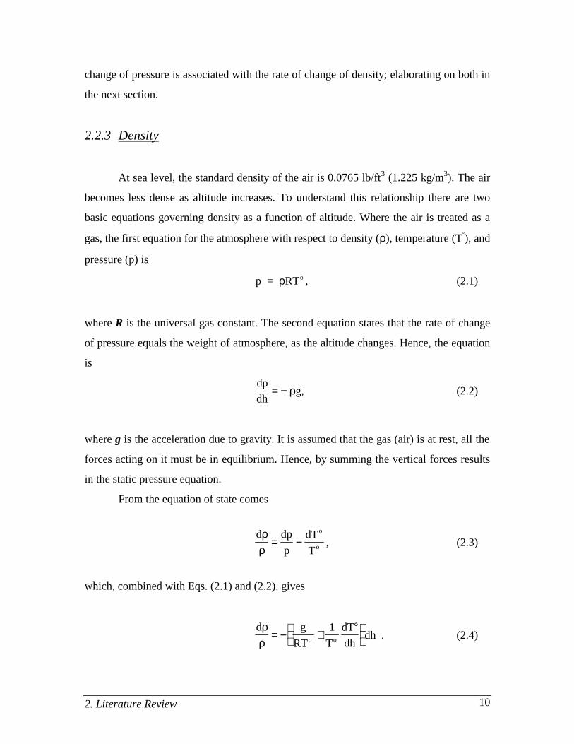
2.2.3 Density
At sea level, the standard density of the air is 0.0765 lb/ft3 (1.225 kg/m3). The air
becomes less dense as altitude increases. To understand this relationship there are two
basic equations governing density as a function of altitude. Where the air is treated as a
gas, the first equation for the atmosphere with respect to density (ρ), temperature (T°), and
pressure (p) is
p = ρRTo , (2.1)
where R is the universal gas constant. The second equation states that the rate of change
of pressure equals the weight of atmosphere, as the altitude changes. Hence, the equation
is
dp
dh= − ρg, (2.2)
where g is the acceleration due to gravity. It is assumed that the gas (air) is at rest, all the
forces acting on it must be in equilibrium. Hence, by summing the vertical forces results
in the static pressure equation.
From the equation of state comes
d dp
p
dT
T
o
o
ρρ
= − , (2.3)
which, combined with Eqs. (2.1) and (2.2), gives
d g
RT T
dT
dhdho o
ρρ
= − +
°
1 . (2.4)
2. Literature Review 11
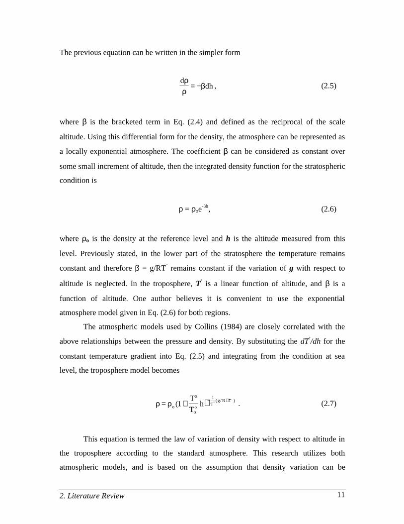
The previous equation can be written in the simpler form
ddh
ρρ
β= − , (2.5)
where β is the bracketed term in Eq. (2.4) and defined as the reciprocal of the scale
altitude. Using this differential form for the density, the atmosphere can be represented as
a locally exponential atmosphere. The coefficient β can be considered as constant over
some small increment of altitude, then the integrated density function for the stratospheric
condition is
ρ = ρoe-βh, (2.6)
where ρo is the density at the reference level and h is the altitude measured from this
level. Previously stated, in the lower part of the stratosphere the temperature remains
constant and therefore β = g/RT° remains constant if the variation of g with respect to
altitude is neglected. In the troposphere, T° is a linear function of altitude, and β is a
function of altitude. One author believes it is convenient to use the exponential
atmosphere model given in Eq. (2.6) for both regions.
The atmospheric models used by Collins (1984) are closely correlated with the
above relationships between the pressure and density. By substituting the dT°/dh for the
constant temperature gradient into Eq. (2.5) and integrating from the condition at sea
level, the troposphere model becomes
)ρ ρ= +° − + °°
o oT
g R TT
Th( ( / )1
0
1
. (2.7)
This equation is termed the law of variation of density with respect to altitude in
the troposphere according to the standard atmosphere. This research utilizes both
atmospheric models, and is based on the assumption that density variation can be
2. Literature Review 12
calculated by the linear lapse rate model for altitudes less than or equal to 36,089 feet and
the logarithmic variation model for altitudes greater than 36,089 feet (see Eqs. 2.12,
2.13).
2.2.4 Viscosity
When understanding viscosity, think of it in relation to the flow of a fluid. A
highly viscous fluid has slow moving, thick and sticky characteristics. Where as low
viscous fluids tend to be less glutinous, moving with ease. “Viscosity is in the form of
tangential stress distributed within the fluid whenever there is relative motion. Hence a
velocity gradient exists, in particular where the fluid moves over the surface of the
vehicle. This is measured by the dynamic viscosity, µ, defined as the ratio of viscous
stress to the velocity gradient” (McCormick, 1995). At sea level, the standard coefficient
of viscosity of air is 1.2024x10⁻⁵ lb/ft-sec (1.7894x10⁻⁵ N-s/m2). The coefficient µ,
depends only on its temperature, and decreases as the temperature decreases with altitude
in the troposphere. It becomes constant in the stratosphere.
An explicit formula for computing the value of µ is
µµ o
T
T=
°°+
0 081480723110 4
3 2
..
/
[N-s/m2] . (2.8)
The ratio of µ and the density of the air is named kinematic viscosity:
νµρ
= (2.9)
2.2.4 Sonic Velocity
“The speed of sound is the rate at which a small disturbance on the ambient
condition travels through the air” (Ruijgrok, 1990). It can be shown that the speed of
2. Literature Review 13
sound is related to the lapse rate model and altitude. The speed decreases at a constant
rate up to an altitude of approximately 36,000 feet (11 km), and then remains constant
throughout the lower portion of the stratosphere. It can be found that the speed of sound,
a, is equal to its initial condition ao minus the lapse rate (λ) times the altitude. The
equation is shown below:
( )a a ho= − λ , (2.10)
where ao is the sonic velocity at sea level, and λ is
λ =−6615 5736
36089
. .. (2.11)
Now that the basic understanding of atmospheric properties has been explained,
the next step is to apply these concepts to predict aircraft performance.

2. Literature Review 14
TABLE 1: United States Standard Atmosphere, 1962
Kinematic Speed of Altitude Temperature Pressure Density viscosity sound ft °F R lb/ft2 slugs/ft3 ft2/s ft/s
0 59.0 518.69 2116.2 2.3769E-03 1.5723E-04 661.5
5,000 41.2 500.86 1760.9 2.0482E-03 1.7755E-04 650.0
10,000 23.3 483.04 1455.6 1.7556E-03 2.0132E-04 638.3
15,000 5.5 465.23 1194.8 1.4962E-03 2.2927E-04 626.4
20,000 -12.3 447.43 937.26 1.2673E-03 2.6234E-04 614.3
25,000 -30.2 429.64 786.33 1.0663E-03 3.0168E-04 601.9
30,000 -48.0 411.86 629.66 8.9068E-04 3.4884E-04 589.3
35,000 -65.8 394.08 499.34 7.3820E-04 4.0575E-04 576.4
40,000 -69.7 389.99 393.12 5.8727E-04 5.0560E-04 573.6
45,000 -69.7 389.99 309.45 4.6227E-04 6.4223E-04 573.6
40,000 -69.7 389.99 393.12 5.8727E-04 5.0560E-04 573.6
45,000 -69.7 389.99 309.45 4.6227E-04 6.4223E-04 573.6
U.S.S.A , 1962 - Definition of Standard Atmosphere
A standard atmosphere is a hypothetical vertical distribution of atmospherictemperature, pressure, and density which by international or national agreement istaken to be representative of the atmosphere for the purpose of altimetercalibrations, aircraft design, performance calculations, etc. The internationallyaccepted standard atmosphere is called the International Civil AeronauticalOrganization (ICAO) Standard Atmosphere or the International StandardAtmosphere (ISA). The U.S. Standard Atmosphere, 1962 is in agreement with theICAO Standard Atmosphere up to 65,000 feet altitude. It is ideal air devoid ofmoisture, water, vapor, and dust, and obeys the perfect gas law. It is based uponaccepted standard values of sea level air density, temperature and pressure.

2. Literature Review 15
2.3 Performance Characteristics of Aircraft
The ideal aircraft would be economical to buy, maintain, have a large seating
capacity, and be fuel efficient. It’s highly unlikely for an aircraft to have all of these
characteristics but it is possible to retain a few. The goal in aircraft design is to achieve a
rational balance between vehicle performance in combination with affordability.
To determine aircraft performance during level flight at any point in the flight
path the following Aircraft Fuelburn Model (AFBM) can be utilized. This model uses the
energy balance concept minus the changes in kinetic and potential energies. The energy
balance equation, as previously described in the introduction, is written as
ET = ΠED,
where the thrust energy, ET equals the product of the drag energy, ΠED.
The energy balance equation now becomes
Fn = DCD
where thrust (Fn) equals the Drag (D) multiplied by the Drag Coefficient (CD). Further
explanation of this concept is Section 2.5.
It is important to describe the path profile equations so that the reader can see the
difference of path and point performance. Each of the functional relationships expressed
as energy terms can be related to the aircraft performance and path profile variables as
follows:
∆KE = f(V1, V2, W1, W2),
∆PE = f(h1, h2, W1, W2),
ED = f(ρ, V, Sw, CD, X),
X = f(V, T),
2. Literature Review 16
where
• V1 and V2 are the increment initial and final true airspeeds (TAS) expressed in ft/sec.
• W1, and W2 are the incremental aircraft weight expressed in lb.
• h1, and h2 are the incremental initial and final density altitudes expressed in feet.
• ρ is the incremental density of the atmosphere expressed in lb-sec2/ft.
• T is incremental travel time expressed in sec.
• X is incremental distance expressed in feet.
In the previous relationships, all of the variables are known path profile dependent
except the wing area (Sw [ft2]) and drag coefficient (CD). The wing area (Sw) is known for
each individual aircraft but CD has a unique relationship with the lift coefficient (CL).
Hence, CL must be obtained under specific operating conditions that provide the required
lift; then CD can be determined.
The corresponding kinematic equations governing the aircraft motion in the
vertical plane are
m &V = T - D - W(sinγ),
m &Vγ = L - W(cosγ),
&X = V(cosγ),
h = V(sinγ),
where X is the range, h is the altitude, V is the true airspeed, T is the thrust, D is the drag,
L is the lift, W is the aircraft weight, m is the aircraft mass, and γ is the flight angle.
The motion of an aircraft can be represented by a quasi-steady-state condition
where the velocity (TAS) and altitude change very slowly so that their respective time
derivatives are assumed to be approximately zero (Roskam, 1989b). With these
assumptions, the four equations above reduce to lift-equals-weight and thrust-equals-drag.
2. Literature Review 17
2.4 Advance Fuelburn Model (AFBM) Assumptions
An aircraft path profile can be described by considering the changes in velocity or
true airspeed (V), altitude (h), and time (T). In order to derive the simplest form of the
energy balance equation, the total path profile is divided into increments of approximately
2,000 ft altitude changes in the case of climbs and descents, or approximately 200
seconds during level flight. It has been found that this size increment yields the level of
accuracy desired, when using both actual and performance handbook data. Other
increments can be chosen, based upon accuracy requirements of a particular application.
Additionally, use of increments permits the following simplifying assumptions:
1. An average atmospheric density (ρ) is used for calculations over the
increment.
2. The aircraft weight change over an increment is small as compared to the total
weight, therefore an average weight (W) is used for incremental calculations.
3. The acceleration during an increment is constant (a).
4. The flight path angle (γ) is small, therefore cosγ ≅ 1, or the aircraft weight
equals the required lift.
5. Climb and descent rates are linear in an increment, thus h2 = h1 + GX.
6. Upper wind effects on fuel consumption are not a part of the computational
requirement; therefore the velocity [TAS] equals the ground speed.
7. The functional forms used for lift vs. drag, and thrust over fuel flow, are
sufficient to obtain a good data fit over the desired speed range.
8. The standard US atmospheric conditions apply, thereby permitting the density
variation with altitude to be calculated by using the following equations:
ρ = 0.0023769 (1 - 0.00000688 ∗ h)4.2563 (2.12)
for altitudes equal to or less than 36,089 ft, and
2. Literature Review 18
ρ = 0.0007062 exp36 089
20 8065
,
, .
−
h(2.13)
for altitudes greater than 36,089 ft.
2.5 Advanced Fuelburn Model
The fuelburn of an aircraft basically depends on airframe drag, engine specific
fuel consumption, distance of the route to be flown, vertical flight path and aircraft
weight. The central factor in every aspect of engine development, is to drive down thrust
specific fuel consumption (TSFC), or simply called the specific fuel consumption (SFC).
SFC is a measure of engine efficiency, defined as fuel flow rate in pounds per hour
divided by engine thrust in pounds of force (lb/hr/lb). Hence, the lower the ratio the lower
the fuel flow rate for a given thrust the lower the fuel consumption and more efficient the
engine. The amount of fuel burned by an aircraft is highly variable with respect to the
power plant, in this case (as to the research) its function is of two factors, altitude and
velocity.
To find the energy consumption relations of an aircraft, the energy balance
equation is appropriate and easily understood. It’s expressed as a function of known
variables that are either aircraft-type performance parameters, or path profile variables
(Collins, 1980a). In order to calculate the estimated fuel consumption a relationship is
needed between fuel burn and thrust. The fuelburn model uses this relationship
incorporating the previous functional relationships (Section 2.3) with engine fuel flow
rates. In Chapter 1, Section 1.4 the fuel flow equation represents a series of coefficients
and variables. This section will describe the steps leading up to this equation allowing for
a full understanding of the fuelburn model.
From the generalized relationship the change in kinetic and potential energy will
not be included. Since this is a steady state analysis the terms go to zero. Using this
approach the energy balance equation will now be a point performance equation that can

2. Literature Review 19
estimate the thrust needed to overcome the aircraft drag at any specified point within a
level profile. Thrust can be written as
Fn = 0.5*ρ*Sw*V2*( Ma + Mb*CL2 + Mc*CL
4 ) . (2.14)
Since the lift is equal to the weight it can be expressed as
L = W = 0.5ρSwV2CL, (2.15)
solving for CL:
CL = W/0.5ρSwV2, (2.16)
the drag is also expressed as
D = 0.5ρSwV2CD . (2.17)
Functionally the drag coefficient can be written in terms of the lift coefficient as
CD = f(CL, M),
where the Mach number (M) is considered to be the average Mach number.
At this juncture in time we will no longer associate the AFBM as a path performance
model, and will now be interpreted as a point performance model.
In “Aviation Fuel Consumption Symposium”, Collins et al., 1984, notes that a
great deal of the performance data concerning both an airframe and an engine represents
an approximation of how a typical air vehicle will function. These approximations
represent a blending of theoretical, wind tunnel, and actual flight test results. Therefore
2. Literature Review 20
the accuracy of the fuel burn model is largely determined by the ingenuity and effort that
is exercised in determining the appropriate mathematical functions based on the
performance data. Then these functions are calibrated and verified by utilizing actual
flight test data.
The conception of the fuel consumption model was determined by data sets
consisting of approximately six-hundred data points (for various altitudes, mach numbers
and throttle settings) to derive the equations for each aircraft model. Collins reports that
this implicit model achieves a standard deviation of 1.4% from engine specifications of
the actual consumption’s observed in the field. And an upper limit of 4% difference
between actual and predicted results has been imposed in the derivation of these multi-
variant equations.
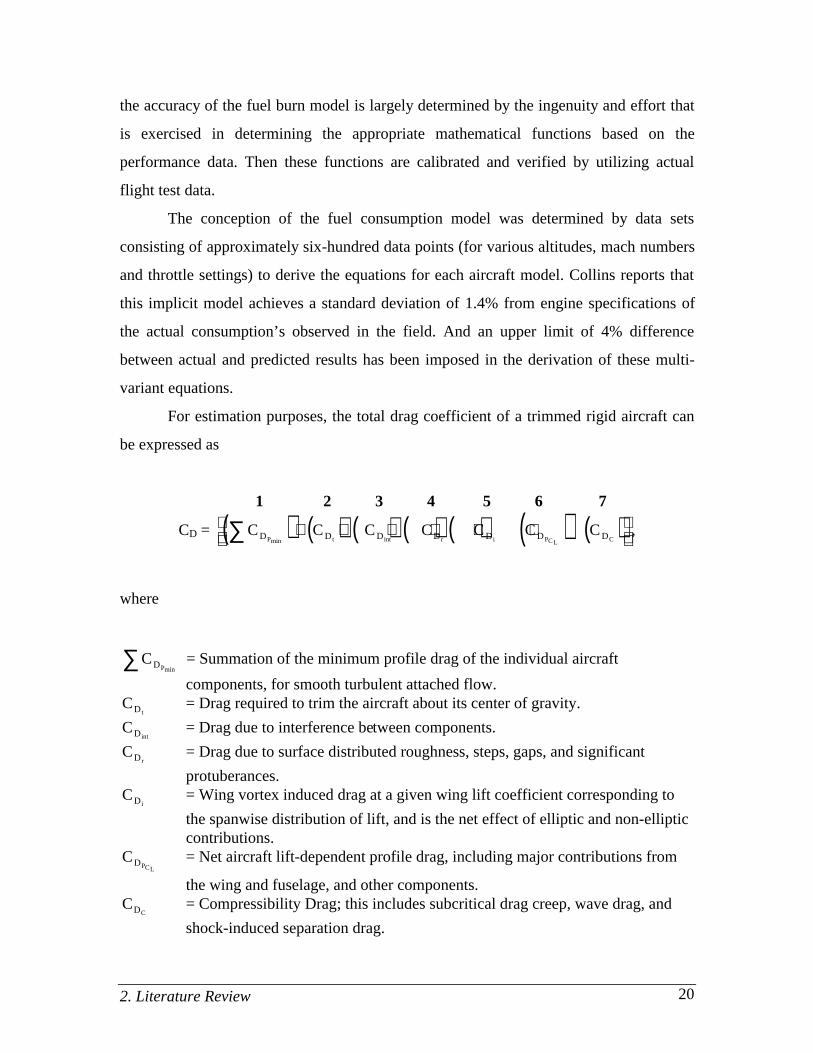
For estimation purposes, the total drag coefficient of a trimmed rigid aircraft can
be expressed as
1 2 3 4 5 6 7
CD = ( ) ( ) ( ) ( ) ( ) ( ) ( )C C C C C C CD D D D D D DP t r i PC L Cmin int∑ + + + + + +
,
where
CDPmin∑ = Summation of the minimum profile drag of the individual aircraft
components, for smooth turbulent attached flow.CDt
= Drag required to trim the aircraft about its center of gravity.
CDint= Drag due to interference between components.
CDr= Drag due to surface distributed roughness, steps, gaps, and significant
protuberances.CDi
= Wing vortex induced drag at a given wing lift coefficient corresponding to
the spanwise distribution of lift, and is the net effect of elliptic and non-ellipticcontributions.
CDPCL
= Net aircraft lift-dependent profile drag, including major contributions from
the wing and fuselage, and other components.CDC
= Compressibility Drag; this includes subcritical drag creep, wave drag, and
shock-induced separation drag.

2. Literature Review 21
The first four terms are not lift dependent, the remaining terms are both lift and
Mach dependent. Collins (1980b) also states that the following functions can be utilized
to present the nondimensional drag coefficient (CD) that consists of a nonlinear drag polar
with sensitivity to Mach number:
CD = Ma + MbC2
L+ McC4
L, (2.18)
where Ma, Mb, and Mc are functions of Mach number representing the first four terms, the
fifth and sixth term, and the last term respectfully.
The three aircraft drag coefficient functions are defined as
Ma = K1 +K2Γ2 + K3Γ4, (2.19)
Mb = K4 +K5Γ + K6Γ2 + K7Γ3 + K8Γ4, (2.20)
Mc = K9 +K10Γ + K11Γ2 + K12Γ3, (2.21)
where Kn is the aircraft specific drag coefficient constant, and Γ is the Mach number ratio.
In Chapter 5, Figure 12 represents plots of Ma, Mb, and Mc vs. Mach number to illustrate
how the influence of drag varies relative to speed.
The model consists of aircraft specific constants and aircraft variables. To
compute the fuel flow over a selected altitude and velocity a technique must be used to
translate thrust into fuel flow. As stated in the introduction the fuel flow (Wf) is
represented by the following empirical relationship:
Wf = F1 + F2Fn + F3Fn2, (2.22)
where F1, F2, and F3 are aircraft fuel flow functions, and expressed as
F1 = C1 + C2M + C3h + C4Mh + C5h2 + C6Mh2, (2.23)
F2 = [C7 + C8M + C9h + C10Mh + C11h2 + C12Mh2](N*104)-1, (2.24)
2. Literature Review 22
F3 = [C13 + C14M + C15h + C16Mh + C17h2 + C18Mh2](N*104)-2 . (2.25)
With the exception of the change in dynamic and kinematic energies, and
configuration changes of the aircraft (landing gear and flap extension) Collins (1984) fuel
burn model utilizes the above core equation to compute the fuel burn. In this case the
current model, AFBM (steady state) might be considered not as sensitive as the original
but a simplified model that utilizes neural network technology. This concept is supposed
to induce further research in the field of aviation fuel consumption via neural networks,
and act as the foundation to more intricate fuel flow studies. Therefore, the object of this
research is to utilize a modeling simulation software in combination with a neural
network to develop a flexible, computationally efficient, and accurate fuel consumption
model that can utilize any aircraft specifics.
2.6 The Power of Neural Networks
Neural networks, or simply neural nets, are computing systems which can be
trained to learn a complex relationship between two or many variables or data sets.
Basically, they are parallel computing systems composed of interconnecting simple
processing nodes (Lau, 1992). Neural net techniques have been successfully applied in
various fields such as function approximation, control systems and signal processing.
Some examples that directly apply to transportation are truck brake diagnosis systems,
vehicle scheduling, and routing systems. In the present application where a certain
relationship exists between a data set of a particular aircraft point profile and its
generalization on all possible data set pairs, neural nets can be used to efficiently predict
the fuel consumption, given velocity and altitude of the vehicle. The data set needed for
the neural net can be an actual steady state flight profile previously recorded or a generic
one provided by an analytical model.
Neural networks utilize a matrix programming environment making most nets
mathematically challenging. It should be understood that it is only the intent here to give

2. Literature Review 23
the reader a brief synopsis of neural networks, and describe the basic type of neural
network used for the research. For a more in-depth review of the intensive mathematical
derivation and computation of the neural networks please refer to the listed references
mentioned throughout this section.
2.6.1 Elements of the Neural Network Paradigm (Hagan et al. 1996)
The neuron model and the architecture of a neural network describe how a
network transforms its input into output. This transformation can be viewed as a
computation. The model and the architecture each place limitations on what a particular
neural net can compute. The way a network computes its output must be understood
before training methods for the net can be explained.
Each neuron is represented by a vector of weights, a scalar (single real number),
and a bias, and the neuron’s transfer function. The products of the neuron’s inputs and
weights are summed with the neuron’s bias and passed through the transfer function to
get the neuron’s output. Keep in mind this is an implicit description of how a neural
network calculates.
A vector is a useful way to describe a pattern of numbers. For example the pattern
of numbers that describe altitude and velocity (input vectors) and the fuel consumption
(target vector) of an aircraft. Suppose that an aircraft (Boeing 747-100) is at FL360, and
traveling at a true airspeed (TAS) of 280 knots consuming 36,000 pounds of fuel per
hour. This information can be summarized in a vector or ordered list of numbers. In fact,
a vector can have many parameters accompanying multidimensional space creating a very
powerful and influential neural network. The neural net recognizes the input vectors as a
set of weights on the input lines connected to a feedforward enhanced backpropagation
(BP) processing unit (BP is classified as a neural net learning rule, and will be explained
in a further section) that delivers the weighted outcome or target vector, a.
Neurons may be simulated with or without biases. A bias is much like a weight,
except that it has a constant input of 1. The constant biases are used to adjust the fuel
consumption model data (input parameters) into a form that the neural net can handle

2. Literature Review 24
easy. The purpose of the addition bias is to reduce the relative spread of the data for each
net input, n. For example if the sets of input/output range considerably, an addition bias
can be added to all the output to reduce the spread. Decreasing the spread in the data
reduces the training time of the neural net.
The Essential Building Blocks and Methodology of Neural Models
1. A scalar input (p) is transmitted through a connection that multiplies its
strength by the scalar weight (w), to form the product w∗p, again a scalar.
2. The transfer function net input (n), again scalar, is the sum of the weighted
input wp plus an optional bias (b). This sum is the argument of the transfer
function (f).
3. A transfer function, typically a sigmoid function or a linear function, that takes
the argument n and produces the scalar output, a.
During the feedforward process the input vector elements enter the network
through the weight matrix W1. The corresponding bias matrix b1 is added to the weights
generating the net input, n. Appendix D contains the networks weight and bias outputs of
all the aircraft used in this research.
W
w w w
w w w
w w w
R
R
S S S R
=
••
• • • ••
1 1 1 2 1
2 1 2 2 2
1 2
, , ,
, , ,
, , ,
, b
b
b
bS
= •
1 1
2 1
1
,
,
,
For easy association, row indices of the elements of the matrix W and b indicate
the destination neuron associated with that weight and bias, while the column indices
indicate the source of the input for that weight and bias.
Figure 2 depicts a single layer network of S neurons with multiple input vectors,
and shows how the bias effects the net input before going to the transfer function, where
the transfer function is contained in the general neuron.

2. Literature Review 25
Inputs General Neuron
WW n n
ff
ppp(1)
p(2)
p(R)
p(1)
p(2)
p(R)
a a
a = f(Wp + b)a = f(Wp + b)
S*RS*R
S*1S*1 S*1S*1
S*1S*1
++
R*1R*1
11 bb
FIGURE 2: Layer of S Neurons with R Inputs
The net input of Figure 2 can be calculated from the summed weight inputs plus a
bias to form the equation:
n = w1,1 p1 + w1,2 p2 + ⋅⋅⋅ + w1,R pR + b .
This expression can be written in matrix form:
n = Wp + b,
where the matrix W for the single-layer case can have multiple S neurons in that layer.
The neuron output is calculated as:
a = f(Wp + b) .
If, for instance, w1,1 = 3, p1 = 2 , w1,2 = 4, p2 = 1and b = -1.5, then
a = f(w1,1 p1 + w1,2 p2 + b)
= f(3(2) + 4(1) - 1.5)
a = f(8.5)
The actual output a, influenced by the bias, depends on the transfer function. Let it
be known that w and b are both adjustable scalar parameters of the neuron. Typically,
2. Literature Review 26
after the transfer function is chosen the parameters w and b will be adjusted by some
learning rule so that the neuron input/output relationship meets some specific goal.
2.6.2 Network Architecture (Hagan et al.,1996)
Neurons that receive the same inputs and use the same transfer function may be
grouped in layers. Layers of neurons may contain any number of neurons and use any
transfer function. Layers may receive input from vectors presented to the network directly
or from outputs of other layers. In BP, networks often have one or more layers of sigmoid
neurons followed by an output layer of linear neurons. A multiple-layer neural net with
nonlinear/linear transfer functions allow the network to learn nonlinear and linear
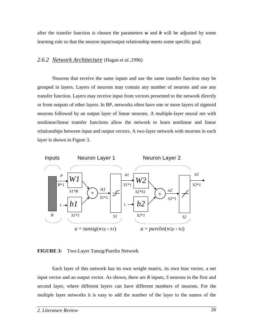
relationships between input and output vectors. A two-layer network with neurons in each
layer is shown in Figure 3.
Inputs Neuron Layer 1 Neuron Layer 2
W1
S1*1
P a1
S1*R
1
a = tansig(W1p + b1)
R*1
R
b1
S1
+
S1*1
n1
1
W2
b2
S2*S1
S2*1
+n2
S2*1
a2
S1*1 S2*1
S2
a = purelin(W2p + b2)
FIGURE 3: Two-Layer Tansig/Purelin Network
Each layer of this network has its own weight matrix, its own bias vector, a net
input vector and an output vector. As shown, there are R inputs, S neurons in the first and
second layer, where different layers can have different numbers of neurons. For the
multiple layer networks it is easy to add the number of the layer to the names of the
2. Literature Review 27
matrices and vectors associated with that layer. Hence, the weight matrix and output
vector for layer two is denoted as W2 and a2 respectively.
This network can be used for general function approximation. It has been proven
that two-layer networks, with sigmoid transfer functions in the hidden layer and linear
transfer functions in the output layer, can approximate virtually any function of interest to
any degree of accuracy, provided a sufficient amount of hidden units are available
[Hoescht, 1989]. Therefore, the neuron model key component, the transfer function, is
used to design the network and established its behavior. Since a multilayer net is more
desirable for this research, the rest of the literature review will be devoted to two-layer
neural nets. Now that the basic methodology of the neuron model is stated, lets look at the
transfer functions.
2.6.3 Transfer Functions (Hagan et al.,1996)
The transfer function may be linear or a nonlinear function of n. And in the case
of multiple neurons, there can be linear and/or nonlinear functions, much like the neuron
model in Figure 3. A particular transfer function is chosen to satisfy some specification of
the problem that the neuron is attempting to solve. There are many common transfer
functions, all of which are applied the same way and are capable of handling batches of
multiple vectors at a time. Some common transfer functions are listed below:
tansig hyperbolic tangent sigmoid
purelin linear
logsig log sigmoid
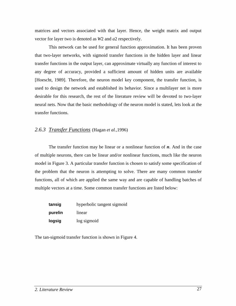
The tan-sigmoid transfer function is shown in Figure 4.
2. Literature Review 28
-b /W
a a
a = tansig (n )
-1
a = tansig (W p + b)
+ 1
0n p
+ 1
0
-1
FIGURE 4: Tan-Sigmoid Transfer Function
For example, the following function calculates the output vector a of a layer of
hyperbolic tangent sigmoid neurons given a network input vector p, the layer’s weight
matrix W and bias vector b, and denote by
a = tansig(Wp + b).
This transfer function takes the input vector of any value between plus and minus
infinity, and squashes the output into the range -1 to 1, according to the expression:
ae e
e e
n n
n n=−+
−
− .
The linear transfer function purelin has output equal to its input, according to the
expression:
a = n .
If the last layer of a BP network has sigmoid neurons then the outputs of the
network are limited to a small range. If linear output neurons are used the network
outputs can take on any value.
The tansig/purelin transfer functions are differentiable and they are also
monotonic increasing functions. Differentiable indicates that if the derivative of the
2. Literature Review 29
function a exists, then the function is differentiable at a. That is, the derivative of the
transfer function must exist at all net outputs, and be monotonic because the output of
each function increases as its input increases. Thus, the transfer functions have no
minima, which would tend to cause error minimum that could trap the network as it
learned.
2.6.4 Backpropagation (Hagan et al.,1996)
One of the primary concerns pertaining to this research was trying to decide which
learning algorithm would be best for the fuel consumption neural net model. The answer
was BP. A basic reference on this subject is “Learning Internal Representations by Error
Propagation”, Rumelhart et al., 1986.
BP was created by generalizing the Widrow-Hoff learning rule (Widrow-Hoff,
1960) known as the delta rule or the Least Mean Square (LMS) method, where it
involves gradient descent techniques in which the performance index is mean square
error (MSE). Gradient descent is the technique where parameters such as weight and
biases are moved in the opposite direction to the error gradient. Each step down the
gradient results in smaller errors until an error minima is reached. During training, the
network parameters (weights and biases) are adjusted in an effort to optimize the
“performance” of the network. A performance surface is created through optimization
containing the minima and maxima points generated by the function parameters. The rule
is an illustration of supervised training, where the net learns in the presence of a
“teacher”. The teacher is based on the level of hidden layers that’s responsible for
learning an associative map between the input level and the output level. The input is
taught to accommodate changes and appropriately alter the output layer. As each input is
applied to the net, the network output is compared to the target. The algorithm will adjust
the weights and biases of the net in order to minimize the MSE, where the error is the
difference between the target output and the network output. Hence, the rule is applied to
a set of pairs of input and target output patterns being associated.
2. Literature Review 30
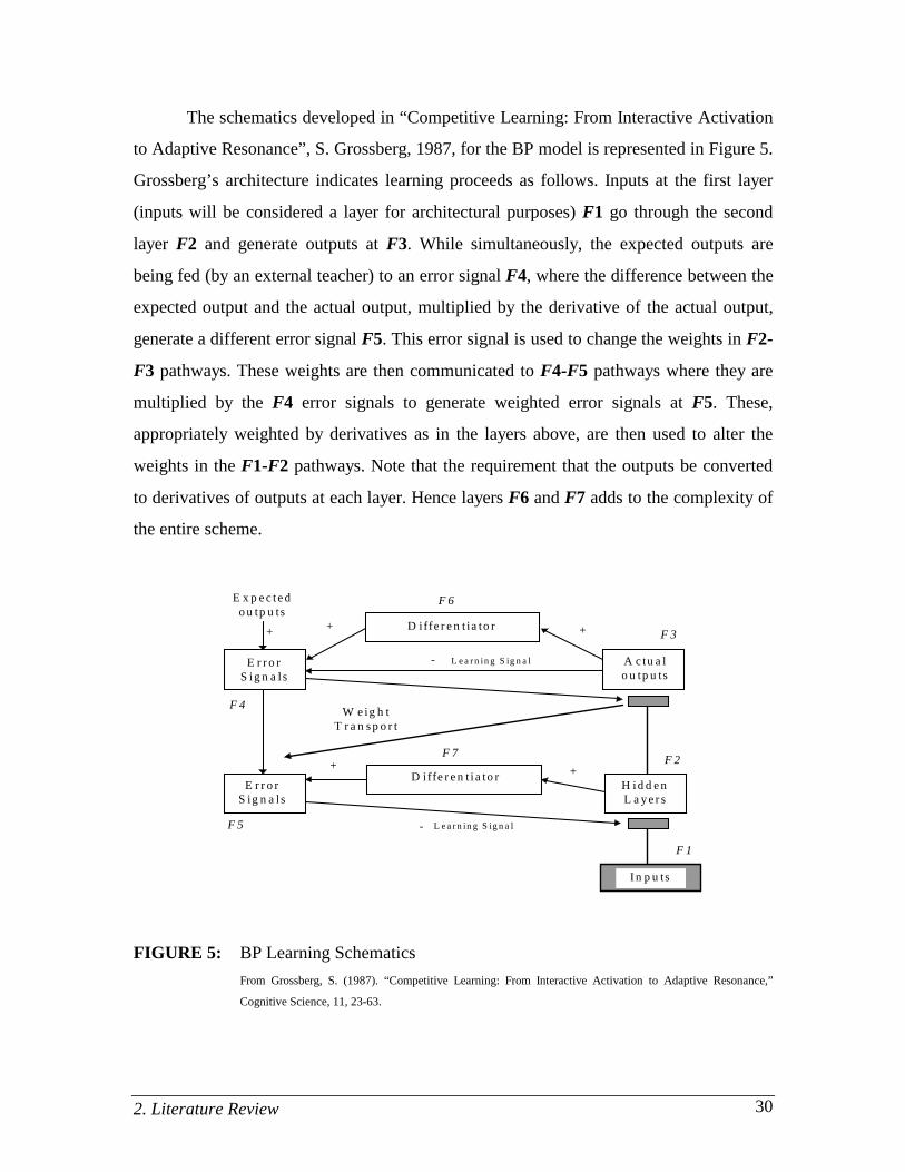
The schematics developed in “Competitive Learning: From Interactive Activation
to Adaptive Resonance”, S. Grossberg, 1987, for the BP model is represented in Figure 5.
Grossberg’s architecture indicates learning proceeds as follows. Inputs at the first layer
(inputs will be considered a layer for architectural purposes) F1 go through the second
layer F2 and generate outputs at F3. While simultaneously, the expected outputs are
being fed (by an external teacher) to an error signal F4, where the difference between the
expected output and the actual output, multiplied by the derivative of the actual output,
generate a different error signal F5. This error signal is used to change the weights in F2-
F3 pathways. These weights are then communicated to F4-F5 pathways where they are
multiplied by the F4 error signals to generate weighted error signals at F5. These,
appropriately weighted by derivatives as in the layers above, are then used to alter the
weights in the F1-F2 pathways. Note that the requirement that the outputs be converted
to derivatives of outputs at each layer. Hence layers F6 and F7 adds to the complexity of
the entire scheme.
E x p e c t e do u tp u ts
+
E r r o rS ig n a ls
F 4
E r r o rS ig n a ls
F 5
+
D iffe r e n t i a to r
F 7+
A c tu a lo u tp u ts
+
H i d d e nL a y e r s
+
F 3
F 2
I n p u ts
F 1
W e ig h tT r a n s p o r t
L e a rn in g S ig n a l-
- L e a rn in g S ig n a l
D i ffe r e n t ia to r
F 6
FIGURE 5: BP Learning Schematics
From Grossberg, S. (1987). “Competitive Learning: From Interactive Activation to Adaptive Resonance,”
Cognitive Science, 11, 23-63.
2. Literature Review 31
Much like the LMS, BP differs only in the way the error derivatives are
calculated. For the multi-layered case the relationship between the network weights and
error is an indirect function of the weights in the hidden layers, they are not directly
proportional. In order to calculate the derivatives the chain rule of calculus is needed (See
Saltz, 1974). Typically, a new input will lead to an output similar to the correct output for
input vectors used in training that are similar to the new input being presented. This can
be termed a generalization property which makes it possible to train a network on a
representative set of input/target pairs and get satisfactory results without training the
network on all possible input/output pairs.
When using the normal BP algorithm, it was determined that it was not sufficient
enough to train and produce an acceptable level of computation. The algorithm when
applied to the large sets of data developed poor results and lengthy training times.
Therefore a variation of the BP was used and called the Levenberg-Marquardt
Backpropagation (LMBP).
2.6.5 Levenberg-Marquardt Backpropagation Algorithm (Hagan et al.,1996)
Training feedforward BP neural nets to minimize mean squared errors is a
numerical optimization technique. The LMBP is a powerful optimization technique was
introduced to the neural net research because it provided methods to accelerate the
training and convergence of the algorithm (Scales, 1985). LMBP is a variation of
Newton’s method that was designed for minimizing functions that are sums of squares of
other nonlinear functions. It utilizes the BP procedures in which derivatives are processed
from the last layer of the network to the first. Like the variation from LMS to BP, BP’s
variation to LMBP differs between the way in which the resulting derivatives are used to
update weights. This algorithm is well suited for neural net training where the
performance index is the MSE.
Developed hundreds of years ago by scientists and mathematicians, the basic
principles of optimization were rediscovered to be implemented on high speed computers.
In conjunction with the optimization theory, neural nets apply the theory to their training
2. Literature Review 32
process. Optimization is an important part of LMBP. The LMBP algorithms role is to
optimize a performance index F(x) or find the value of x that minimizes F(x). In general
the optimization begins with some initial guess, x0 and then updated versions of the guess
through iterations are found according to an equation of the form
xk+1 = xk + αkpk , (2.26)
or
∆xk = (xk+1 - xk) = αkpk .
where the vector pk represents a search direction and the learning rate, αk, which
determines the length of the step.
For this research the value x that minimizes F(x) is given by the input vectors and
biases (performance index; PI)
The Methods to Accelerate the Convergence of Standard BP
• Enhanced Optimizing Techniques
Approximate Steepest Descent Rule
Gauss-Newton Method
Once the optimum (minimum) point of x that minimizes the F(x) is found by Eq. 2.26, its
desired to have the F(x) decrease at each iteration. In other words,
F(xk+1) < F(xk) . (2.27)
In order for the “descent” to occur, pk must interact with a small learning rate, αk. The
first-order-Taylor series is used as follows
F(xk+1) = F(xk + ∆xk) = F(xk) + gTk∆xk ,
2. Literature Review 33
where: gTk is the gradient evaluated at the first value of x that minimizes the F(x).
The gradient vector:
g F xk x xk= ∇ =( ) . (2.28)
To satisfy Eq. 2.27 the second term on the right hand side of Eq. 2.28 must be negative
gTk∆xk = αkg
Tkpk < 0 .
In general it is best to select a small learning rate, αk, as this will improve the search
direction.
This implies:
gTkpk < 0.
Therefore, using this logic along with the iteration of Eq. 2.26 produces the steepest
descent method:
xk+1 = xk - αkgT
k .
The Gauss-Newton method is based on the second-order Taylor series. This
method will always find the minimum of a quadratic function in one step. It is designed to
approximate a function as quadratic and then locate the stationary point of the quadratic
approximation. If the original function is quadratic (with a strong minimum) it will be
minimized in one step. If the original function F(x) is not quadratic then the method will
not generally converge in one step.
Second-order Taylor series:
F(xk+1) = F(xk + ∆xk) = F(xk) + gTk∆xk + 1/2∆xT
kAk∆xk , (2.29)
2. Literature Review 34
Use ∇F(x) = Ax + d to take the gradient of Eq. 2.29 with respect to ∆xk and set it equal to
zero to get gk + Ak∆xk = 0.
Solving for ∆xk produces
∆x A gk k k= − −1 .
Newton’s method for optimizing a performance index F(x) is
x x A g .k+ k k k11= − − (2.30)
where A F xk x xk≡ ∇ =
2 ( ) and g F xk x xk≡ ∇ =( ) .
If we assume that F(x) is the sum of squares function:
F x v x x xiT
i
N
( ) ( ) ( ) ( ),= ==∑ 2
1
v v
then the jth element of the gradient would be
[ ]∇ = ==∑F x
F x
xv x
v x
xjj
ii
ji
N
( )( )
( )( )
.∂∂
∂∂
21
The gradient can therefore be written in matrix form:
∇ =F x x v x( ) ( ) ( ).2J T (2.31)
where J is the Jacobian matrix and depicted as

2. Literature Review 35
J( )
( ) ( ) ( )
( ) ( ) ( )
( ) ( ) ( )
x
x
x
x
x
x
xx
x
x
x
x
x
x
x
x
x
x
x
n
n
N N N
n
=
∂∂
∂∂
∂∂
∂∂
∂∂
∂∂
∂∂
∂∂
∂∂
v v v
v v v
v v v
2
1
1
1
2
1
2
1
2
2
1 2
L
L
M M M
L
.
The next step is finding the Hessian matrix. The k,j element of the Hessian matrix
would be
[ ]∇ = = +
=∑2
2 2
1
2F xF x
x x
v x
x
v x
xv x
v x
x xk jk j
i
k
i
ji
i
k ji
N
( )( ) ( ) ( )
( )( )
.,
∂∂ ∂
∂∂
∂∂
∂∂ ∂
The Hessian matrix can then be expressed in matrix form:
∇ = +2 2 2F x x x x( ) ( ) ( ) ( ),J J ST
where
S( ) ( ) ( ).x v x v xii
N
= ∇=∑ 1
2
1
If we assume that S(x) is small, we can approximate the Hessian matrix as
∇ ≅2 2F x x x( ) ( ) ( ).J JT (2.32)
By substituting Eq. (2.32) and Eq. (2.31) into Eq. (2.30), we obtain the Gauss-Newton
method:
2. Literature Review 36
[ ][ ]
x x x x x x
x x x x x
k x k k k k
x k k k k
+−
−
= −
= −
1
1
1
2 2J J J J
J J J J
T T
T T
( ) ( ) ( ) ( ).
( ) ( ) ( ) ( )
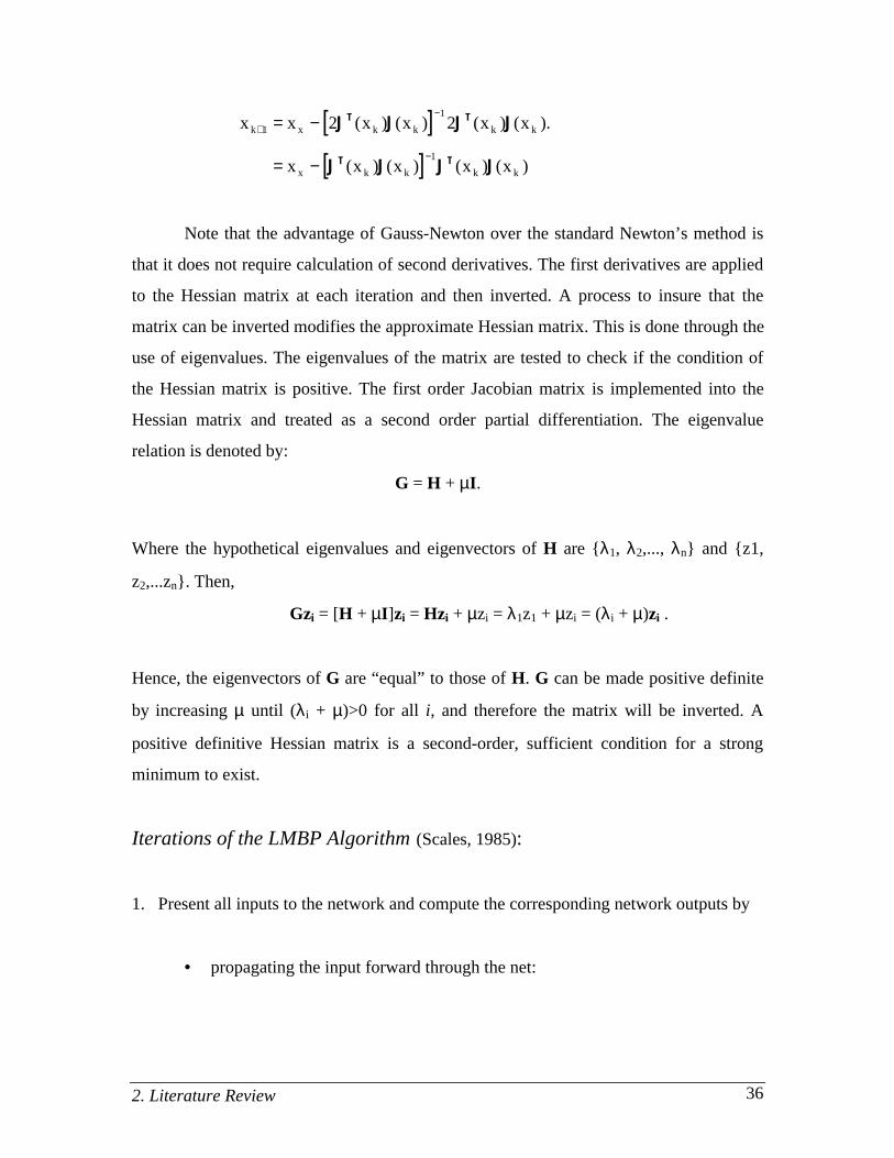
Note that the advantage of Gauss-Newton over the standard Newton’s method is
that it does not require calculation of second derivatives. The first derivatives are applied
to the Hessian matrix at each iteration and then inverted. A process to insure that the
matrix can be inverted modifies the approximate Hessian matrix. This is done through the
use of eigenvalues. The eigenvalues of the matrix are tested to check if the condition of
the Hessian matrix is positive. The first order Jacobian matrix is implemented into the
Hessian matrix and treated as a second order partial differentiation. The eigenvalue
relation is denoted by:
G = H + µI.
Where the hypothetical eigenvalues and eigenvectors of H are {λ1, λ2,..., λn} and {z1,
z2,...zn}. Then,
Gzi = [H + µI]zi = Hzi + µzi = λ1z1 + µzi = (λi + µ)zi .
Hence, the eigenvectors of G are “equal” to those of H. G can be made positive definite
by increasing µ until (λi + µ)>0 for all i, and therefore the matrix will be inverted. A
positive definitive Hessian matrix is a second-order, sufficient condition for a strong
minimum to exist.
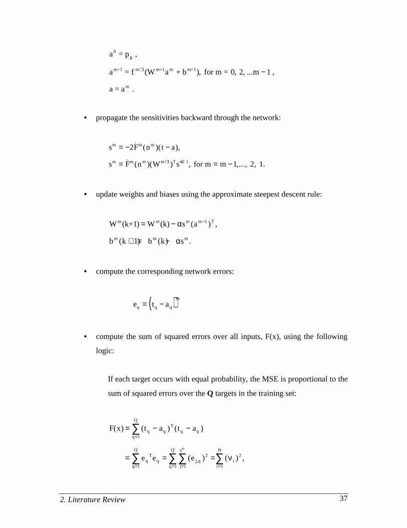
Iterations of the LMBP Algorithm (Scales, 1985):
1. Present all inputs to the network and compute the corresponding network outputs by
• propagating the input forward through the net:
2. Literature Review 37
a = p ,
a = f (W a + b ) for m = , , ...m ,
a = a .
g
m+ m m+ m m+
m
0
1 1 1 1 0 2 1+ −,
• propagate the sensitivities backward through the network:
s F n t a
s F n W s m
m m m
m m m m T m
= − −
= = −+ +
2
11 1
& ( )( ),
& ( )( ) , for m ,..., 2, 1.
• update weights and biases using the approximate steepest descent rule:
W (k+ ) W (k) s a
b k b k s
m m m m T
m m m
1
1
1= −
+ = −
−α
α
( ) ,
( ) ( ) .
• compute the corresponding network errors:
( )e t aq q q
m
= −
• compute the sum of squared errors over all inputs, F(x), using the following
logic:
If each target occurs with equal probability, the MSE is proportional to the
sum of squared errors over the Q targets in the training set:
F x t a t a
e e e
q qq
QT
q q
qT
Q
j qj
s
q
Q
ii
Nm
( ) ( ) ( )
( ) ( ) ,,
= − −
= = =
=
= == =
∑
∑ ∑∑ ∑
1
1
2
11
2
1
ν

2. Literature Review 38
where ej,q is the jth element of the error for the qth input/target pair.
2. The key step in the LMBP algorithm is the computation of the Jacobian matrix. To
create the matrix we need to compute the derivatives of the errors.
• the form of the matrix is presented by a parameter vector:
[ ] [ ]x Tn= =χ χ χ1 2K K K Kw w w b b w b1,1
11,21
S ,R
111
S
11,12
S
M1 1 M ,
N = Q x SM and n = S1(R + 1) + S2(S1 + 1) + K + SM(SM-1 + 1).
and an error vector:
[ ] [ ]v Tn Q
= =ν ν ν1 2K K Ke e e e e1,1 2,1 S ,1 1,2 SM M ,.
• calculate the sensitivities with the recurrence relations:
The BP process computes the sensitivities through a recurrence relationship from
the last layer backward to the first layer. When the input pq has been applied to the
network and the corresponding output aqM has been computed, the LMBP is
initialized with
~ & ( )S FqM M M= − nq ,
where: & ( )FM Mnq is the matrix of the function, f, that is an explicit function only of the
variable n.

2. Literature Review 39
& (
& )& )
& )& )
FM n
f n
f n
f n
f n
M
1M
2M
3M
S
M
)
( 0
(
(
0 ( M
=
L
L
M M M
0
0 0
0 0
Each column of the matrix ~Sq
M must be backpropagated through the net using the
final recurrence relation for the sensitivity: Using the Chain rule in matrix form
and denoted as
~ $ $& ( )( )
$S
F FF
FM
T
M T= =
=
∂∂
∂∂
∂∂
∂∂n
n
n nn
nM
M+1
M M+1M M+1
M+1W ,
Therefore to produce one row of the Jacobian matrix, the columns can be BP
together using:
~ & ( )(~
S F W SqM M M M M= + +n 1 1 )T .
The total Marquardt sensitivity matrices for each layer are created by augmenting
the matrices computed for each input:
[ ]~ ~ ~ ~S S S SM M M
QM= 1 2 K .
Note that for each input the net will backpropagate SM sensitivity vectors. This is because
derivatives are computed for each individual error, rather than the derivative of the sum
of squares of the errors. For every input applied to the net there will be SM errors, for each
error, there will be one row of the Jacobian matrix.
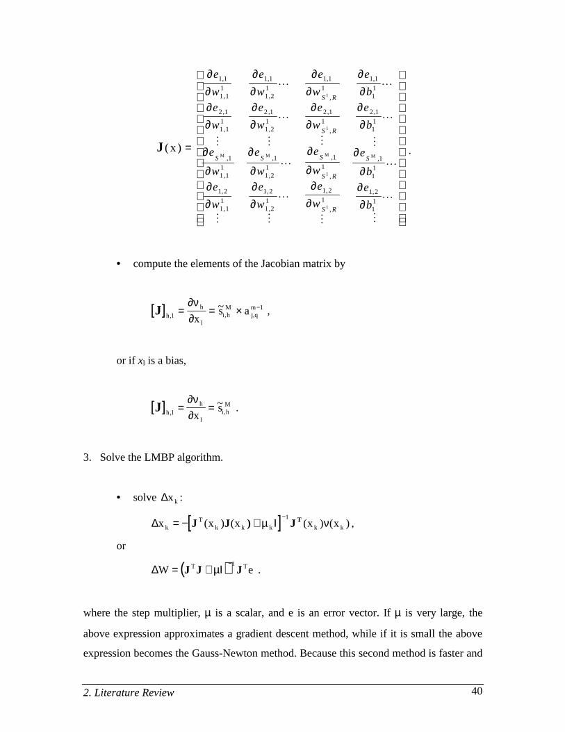
2. Literature Review 40
J ( )
, , , ,
, , , ,
, , , ,
, ,
x =
∂∂
∂∂
∂∂
∂∂
∂∂
∂∂
∂∂
∂∂
∂
∂
∂
∂
∂
∂∂
∂∂∂
∂∂
e
w
e
w
e
w
e
be
w
e
w
e
w
e
b
e
w
e
w
e
w
e
be
w
e
S R
S R
S S S
S R
S
1 1 1 1 1 1 1 1
2 1 2 1 2 1 2 1
1 1 1 1
1 2 1 2
1,11
1,21
,
111
1,11
1,21
,
111
1,11
1,21
,
111
1,11
1
1
M M M
1
M
L L
L L
M M
L
M M
L
Mw
e
w
e
bS R1,21
,
11
11
1
L
M M
L
M
∂∂
∂∂
1 2 2, ,
.
• compute the elements of the Jacobian matrix by
[ ]J h lh
li hM
j qm
xs a, , ,~= = × −∂ν
∂1 ,
or if xl is a bias,
[ ]J h lh
li hM
xs, ,~= =
∂ν∂
.
3. Solve the LMBP algorithm.
• solve ∆x k :
[ ]∆ Ιx x x x xk k k k k k= − +−
J J ) J TT ( ) ( (µ ν1
) ( ) ,
or
( )∆W e= +−
J J JT TµΙ1
.
where the step multiplier, µ is a scalar, and e is an error vector. If µ is very large, the
above expression approximates a gradient descent method, while if it is small the above
expression becomes the Gauss-Newton method. Because this second method is faster and

2. Literature Review 41
more accurate near an error minimum so the aim is to shift towards the Gauss-Newton
method as quickly as possible. Thus, µ is decreased after each successful step and
increased only when a step increases the error.
4. Recompute the sum of squared errors using (xk + ∆xk). If the sum of squares is
smaller than that of step 1, divide µ by a step multiplier factor,ϑ, let xk+1 = xk + ∆xk
and go back to step 1. If the sum of squares is not reduced, then multiply µ by ϑ and
go back to step 3.
The LMBP algorithm converges when the norm of the gradient is less than the
predetermined value or when the sum of squares has been reduced to some error goal.
The main draw back of LMBP is the storage requirement. The JTJ matrix, which
must be inverted, is n x n, where n is the total number of weights and biases in the
network. If the network has more than a few thousand parameters, the LMBP algorithm
becomes impractical on current computers.
3. Methodology 42
3. METHODOLOGY
3.1 Introduction
This chapter describes the methodology used for conducting this research. The
main objective of the methodology is to develop a realistic, easily implemented, efficient
method for fuel consumption modeling through neural network applications. With the use
of optimization, finding the value of weights and biases that minimize the F(x), where x
is the scalar parameter (composed of two variables) that is adjusted each time the neural
net iterates, a model can be developed to calculate fuel consumption at any velocity and
altitude desired. This chapter briefly describes the development of the fuel consumption
model, the neural network, the approach to efficient neural networking, and the use of
MATLAB as an optimization tool.
3.2 Models and Nonlinear Optimization
The first step in studying fuel consumption is to identify past techniques used to
model fuelburn of an aircraft. Once this is established the researcher can relate past
techniques with his/her own logic to formulate and build a model. Concisely, a model can
be thought of as a representation of parts that when combined and work with each other
create a whole, in this case the whole is fuel consumption. A model is used to investigate
possible improvements of the study, and discover the effect of different inputs that could
alter the output. There are many kinds of models. For example, verbal-descriptive,
graphical, mathematical, logical algorithms and computer models. In certain instances a
given study may be best modeled by a culmination of these types. Because of the need to
incorporate numerical data and logic, this fuel consumption model is almost invariably
mathematical and logical algorithm based, and the analysis employs both methods.
3. Methodology 43
A models directive is to satisfy an objective as the purpose of the study. It should
be highly faithful in representing the objective, accurately reproducing its outcome or
predicting the results of hypothetical application. A valid point to make is that a model
can comprise subsystems (submodels) in order to reduce the complexity because
submodels are often easier to define. Good model performance also relies on the level of
detail and nonambiguity of the model.
The model, a neural network fuel consumption model (AFCM), will be compared
to the SIMMOD fuelburn post-processor. It will incorporate two submodels: (1) the
AFBM, (2) a multilayer neural network optimization model (NNOM).
Nonlinear optimization is used because of the nonlinearity of the transfer
functions. This technique, sometimes called continuous-variable nonlinear programming,
involves real decision variables but the objective and constraint functions are not
necessarily linear. The objective of optimization is to train the network parameters (w, b)
so they can be adjusted in an effort to optimize the performance of the network. Neural
nets are taught to accommodate changes in the weights and bias to appropriately
reconfigure the output. Each time it iterates (teaches), the error between the output and
target becomes smaller until a minimized error goal is achieved. The theoretical outlook
for the AFCM should be as follows:
• goal or purpose directed
• understandable and easy to use
• suitable for a wide range of aircraft
• easy to modify or update the model
The whole idea for this research stemmed from SIMMOD. Looking for ways to
make the software operate more efficiently incorporating a different approach in
calculating fuelburn. For this model to be useful the above statement must be satisfied
including the ability for the model to be implemented into SIMMOD or any
airport/airspace simulation software. Although the model is not dynamic in nature relative
3. Methodology 44
to SIMMOD’s AFBM, it can be incorporated into the software so that it will be
recognized to compute fuelburn at every point in the flight path.
3.3 Approach to Model Development
A successful study is related to the methodology used by the modeller and his/her
knowledge of the platform and expertise in the analysis of the topic in question. It is
usually better to have a plan before starting modeling. The following activities or steps
are applied in this research to compose a sound fuel consumption model.
• Problem Formulation. Successful problem formulation is the most critical step
in developing a model. The first issue is to bound the problem, to gather all the
information critical to the overall objective.
• Data Collection and Analysis. Information and data needed by the fuel
consumption model should be identified and collected. The data needed is
Specific Aircraft Coefficients that come from Bela Collins AFBM
Velocity, Altitude and Fuelflow generated from the AFBM
All parameters and variables that affect the measure of fuelburn such as atmospheric
properties are also to be identified. The AFBM will be the base model that the neural
network will try to map. Once that is done the neural net will generalized fuel
consumption data within the parameters defined by the base model. After the
generalization process the new data is then implemented back into the base model to be
compared with the generalized data. If the data comparison is a success then fuel
consumption can be estimated at specific velocities and altitudes for that particular
aircraft.
• Model Development. The AFCM consists of two major subsystem models: The
AFBM, which performs the initial fuel consumption calculations and termed the
3. Methodology 45
“fuelburn calculator”, and the NNOM, which utilizes the initial velocity, altitude and fuel
consumption data from the AFBM to mimic the fuel consumption.
In order to formulate the subsystem models into the AFCM an explicit approach is
used to analyze each segment of the models. This method is used to define the individual
algorithms or information entities through the model on the basis of sequence of events
that occur in a pre-defined pattern.
This research can be broadly divided into two parts: (1) determining a velocity
and altitude profile that generates fuel consumption, and (2) invoking that data into a well
defined neural network. The detail of this logic will be presented in Chapter 4. After
formulation the subsystem models will be tested together in the MATLAB environment.
The next step is to combine the models to form a single model (AFCM). It is necessary
for the modeller to chose aircraft specific data that corresponds to the desired aircraft
being modeled. It maybe useful to run the AFBM with the selected aircraft data in order
to verify the accuracy of the model before combining it with the NNOM. In this step, it is
also important to delete any ambiguity within the data output. For example, if the output
shows that the aircraft travels at some velocity and altitude consuming fuel at an
unbelievable rate, then these outliers can be removed from the data base. The following
represents an example of the ambiguous case:
Type Aircraft: MD-80
Velocity: 500 knots (IAS)
Altitude: 44,000 feet
It would not be feasible for this aircraft to travel at these parameters.
• Validation and Modification of Models. The validity of models is a measure of
the extent to which the parameters satisfy the study objectives. Validation involves
conducting a series of tests on the input, output, and structure of the model. Common
methods for validating are to compare the output of the model(s) to initial data under
similar environmental conditions and to check the reliability of the output. Basically, if
the output is similar the final model is accepted as a realistic representation for the
3. Methodology 46
research. The following output from the AFCM is used as a measure of effectiveness for
comparison with the generalized AFBM output data: (1) the mean, (2) root-mean-square
(RMS), (3) t-test, (4) confidence interval, and (5) the computation time of the entire
AFBM fuel consumption output compared to the AFCM fuel consumption output. The
ultimate validation of the AFCM is how well it can predict the fuel consumption of an
aircraft with specific input parameters (velocity and altitude).
• Design Experiments and Running the Optimization. In this step it must be
decided what aircraft input variables, and neural net structure to use for the design of the
AFCM. An experimental design requires observations of the submodels under specific
combinations run in the MATLAB environment. For a selected AFCM, some decisions
must be made on certain issues as initial conditions for the AFBM, the neural net design
architecture, and encompassing neural net design parameters. Once these are met the
AFCM can be tested and used in actual aircraft specific scenarios.
• Analysis of Output Data and Implementation. Analysis of the AFCM results is
to achieve the research objectives. This step brings out several important outcomes such
as determination of fuel consumption at a particular point within the flight envelope, the
floating point operations (flops) of the AFBM compared to the neural nets generalization,
and the accuracy of the neural net generalization compared to the generalized AFBM
(GAFBM). The analyst draws inferences from these outcomes and makes specific
recommendations on how the AFCM works and how it could be improved. This is not a
simple process, at a number of points the process may go back to the previous step.
3.4 Aircraft Fuel Consumption Model (AFCM) Assumptions
The AFCM assumptions are based on simplifying the energy balance equation. By
simplifying the equation we get point performance. As stated, the model has been
modified to except only the cruise segment of the profile. With this in mind several of the
assumptions were left out, such as the climb/descent rates and incremental changes in
altitude of approximately 2,000 ft or approximately 200 seconds during level flight.
3. Methodology 47
During level cruise the following is assumed in order to maintain efficient computations
without an unacceptable effect on accuracy:
1. The aircraft weight change at a certain flight level is small compared to the
total weight, therefore total weight is used in the calculations.
2. Acceleration = 0 during any flight level.
3. The flight path angle (γ) is small, therefore cosγ ≅ 1, or the aircraft weight
equals the required lift.
4. Upper wind effects on fuel consumption are not a part of the computational
requirement; therefore the velocity [IAS] equals the ground speed.
5. The functional forms used for lift vs. drag, and thrust over fuel flow, are
sufficient to obtain a good data fit over the desired speed range.
6. The standard US atmospheric conditions apply.
3.5 Description of MATLAB
MATLAB, created by MathWorks Inc. is a powerful and advanced computational
software that handles numeric computation, algorithm prototyping and specific purpose
problem solving with matrix formulations that arise in disciplines such as optimization
and statistics. MATLAB is used for research, solving practical engineering and
mathematical problems. MATLAB 4.0 is the current version of MATLAB used in a
variety of platforms for today’s systems. An updated version 5.0 is due to come out some
time in early 1997. This software has powerful features used toward an array of
disciplines. The toolboxes within MATLAB give this software the versatility needed for
today’s high demand in programming, simulation, and graphing.
A MATLAB NNOM consists of input vectors, target vectors, transfer functions,
learning rates, and sum-square error goals. All of which are very easy to modify and
manipulate. Also to test the sensitivity of the model and have the possibility to
3. Methodology 48
incorporate a graphical user interface (GUI). The following features of MATLAB that are
pertinent to this research are as follows:
1. Solving problems in a fraction of the time it takes to write another program in another
language to produce the same output.
2. Extensive toolboxes to solve particular classes of problems.
3. Easily extensive, allowing you to be the author of the programming, creating your
own applications.
4. Interaction with other programming languages (Fortran, C++).
5. Hierarchical modeling to make complex systems easy to build and understand.
6. On-line help is available from help commands at the MATLAB prompt, and technical
service assistance via e-mail at [email protected]
The powerful features of MATLAB prove to be effective in this research.
3.6 Research Discussion and Pertaining Questions
Modeling software - MATLAB has extensive neural net capabilities. The neural
net is similar to the polynomial approximation structure except the weights of each
coefficient can have specific ways of behaving through the use of a multitude of sigmoid
or linear transformations. Neural networks can contain a series of neurons that posses
input and output layers, where each neural will have a specific weight coefficient and bias
coefficient. Suppose the neural net contains input variables P1 and P2, they effect fuel
consumption by drag forces that are related to the amount of thrust. The output will be
fuel flow, although there can be multiple outputs such as fuel flow and thrust. This
research only requires one output: fuel flow. The aircraft must be kept under certain
conditions, meaning it can move with three degrees of freedom, require certain velocities
and altitudes based on a specific fuel flow.
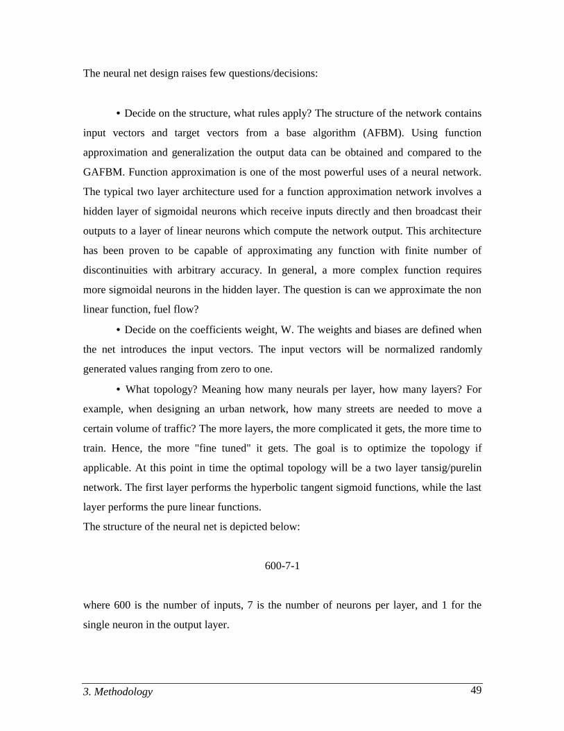
3. Methodology 49
The neural net design raises few questions/decisions:
• Decide on the structure, what rules apply? The structure of the network contains
input vectors and target vectors from a base algorithm (AFBM). Using function
approximation and generalization the output data can be obtained and compared to the
GAFBM. Function approximation is one of the most powerful uses of a neural network.
The typical two layer architecture used for a function approximation network involves a
hidden layer of sigmoidal neurons which receive inputs directly and then broadcast their
outputs to a layer of linear neurons which compute the network output. This architecture
has been proven to be capable of approximating any function with finite number of
discontinuities with arbitrary accuracy. In general, a more complex function requires
more sigmoidal neurons in the hidden layer. The question is can we approximate the non
linear function, fuel flow?
• Decide on the coefficients weight, W. The weights and biases are defined when
the net introduces the input vectors. The input vectors will be normalized randomly
generated values ranging from zero to one.
• What topology? Meaning how many neurals per layer, how many layers? For
example, when designing an urban network, how many streets are needed to move a
certain volume of traffic? The more layers, the more complicated it gets, the more time to
train. Hence, the more "fine tuned" it gets. The goal is to optimize the topology if
applicable. At this point in time the optimal topology will be a two layer tansig/purelin
network. The first layer performs the hyperbolic tangent sigmoid functions, while the last
layer performs the pure linear functions.
The structure of the neural net is depicted below:
600-7-1
where 600 is the number of inputs, 7 is the number of neurons per layer, and 1 for the
single neuron in the output layer.
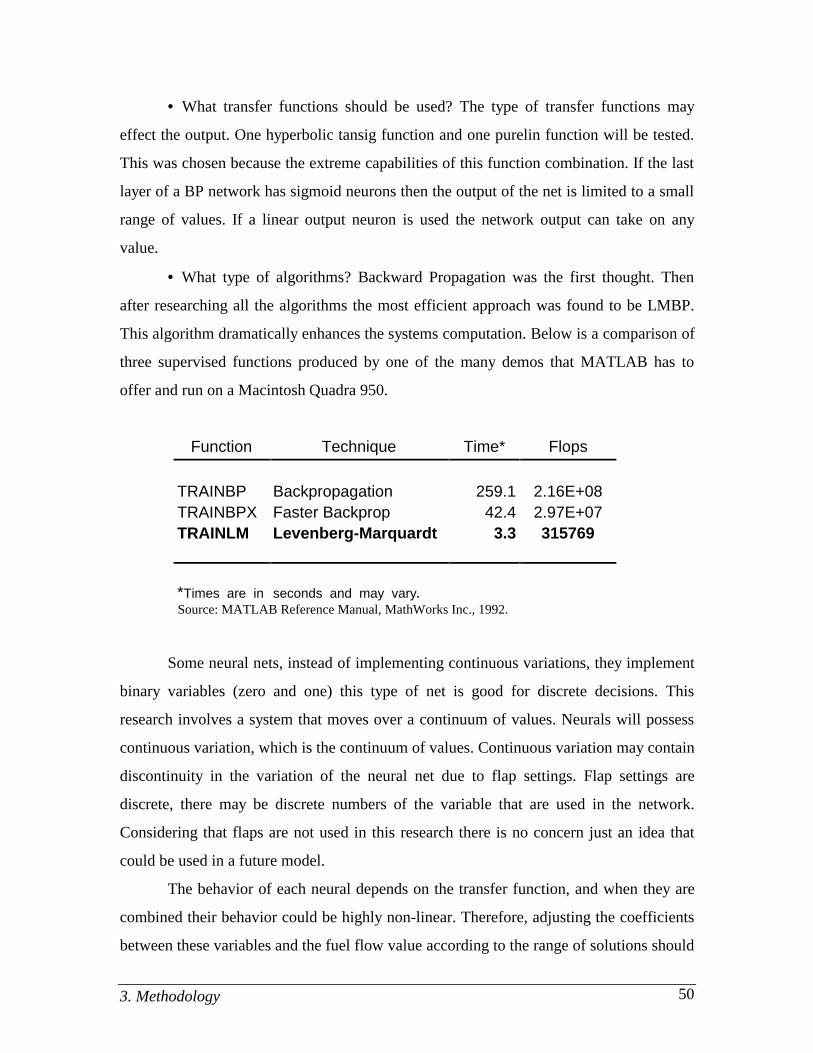
3. Methodology 50
• What transfer functions should be used? The type of transfer functions may
effect the output. One hyperbolic tansig function and one purelin function will be tested.
This was chosen because the extreme capabilities of this function combination. If the last
layer of a BP network has sigmoid neurons then the output of the net is limited to a small
range of values. If a linear output neuron is used the network output can take on any
value.
• What type of algorithms? Backward Propagation was the first thought. Then
after researching all the algorithms the most efficient approach was found to be LMBP.
This algorithm dramatically enhances the systems computation. Below is a comparison of
three supervised functions produced by one of the many demos that MATLAB has to
offer and run on a Macintosh Quadra 950.
Function Technique Time* Flops
TRAINBP Backpropagation 259.1 2.16E+08TRAINBPX Faster Backprop 42.4 2.97E+07TRAINLM Levenberg-Marquardt 3.3 315769
*Times are in seconds and may vary. Source: MATLAB Reference Manual, MathWorks Inc., 1992.
Some neural nets, instead of implementing continuous variations, they implement
binary variables (zero and one) this type of net is good for discrete decisions. This
research involves a system that moves over a continuum of values. Neurals will possess
continuous variation, which is the continuum of values. Continuous variation may contain
discontinuity in the variation of the neural net due to flap settings. Flap settings are
discrete, there may be discrete numbers of the variable that are used in the network.
Considering that flaps are not used in this research there is no concern just an idea that
could be used in a future model.
The behavior of each neural depends on the transfer function, and when they are
combined their behavior could be highly non-linear. Therefore, adjusting the coefficients
between these variables and the fuel flow value according to the range of solutions should
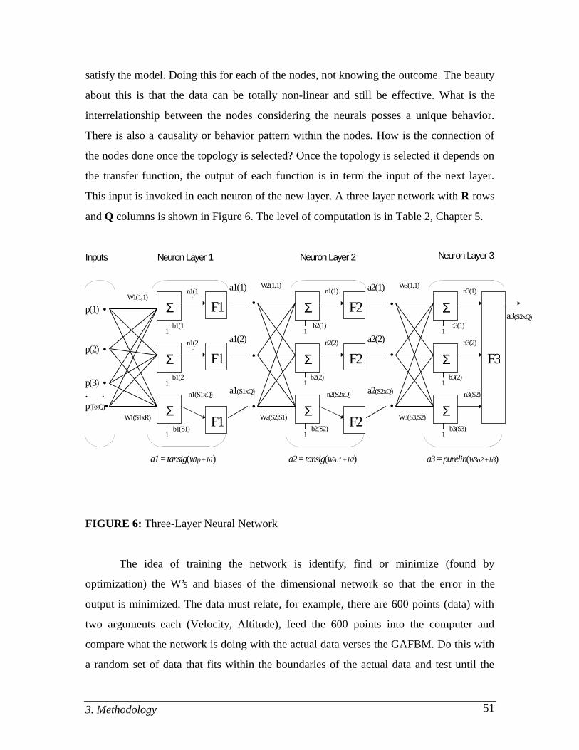
3. Methodology 51
satisfy the model. Doing this for each of the nodes, not knowing the outcome. The beauty
about this is that the data can be totally non-linear and still be effective. What is the
interrelationship between the nodes considering the neurals posses a unique behavior.
There is also a causality or behavior pattern within the nodes. How is the connection of
the nodes done once the topology is selected? Once the topology is selected it depends on
the transfer function, the output of each function is in term the input of the next layer.
This input is invoked in each neuron of the new layer. A three layer network with R rows
and Q columns is shown in Figure 6. The level of computation is in Table 2, Chapter 5.
Inputs Neuron Layer 1
p(1) •
p(2) •
p(3) •. .p(RxQ)•
W1(1,1)
1
n1(1)
a1 = tansig(W1p + b1)
b1(S1)
F1
b1(2
b1(1
n1(2)
n1(S1xQ)
1
1
Σ
Σ
ΣW1(S1xR)
F1
F1
Neuron Layer 2
•
•
•
W2(1,1)
1
n1(1)
a2 = tansig(W2a1 + b2)
b2(S2)
F2
b2(2)
b2(1)
n2(2)
n2(S2xQ)
1
1
Σ
Σ
ΣW2(S2,S1)
F2
F2
a1(1)
a1(2)
a1(S1xQ)
Neuron Layer 3
•
•
•
W3(1,1)
1
n3(1)
a3 = purelin(W3a2 + b3)
b3(S3)
b3(2)
b3(1)
n3(2)
n3(S2)
1
1
Σ
Σ
ΣW3(S3,S2)
a2(1)
a2(2)
a2(S2xQ)
a3(S2xQ)
F3
FIGURE 6: Three-Layer Neural Network
The idea of training the network is identify, find or minimize (found by
optimization) the W’s and biases of the dimensional network so that the error in the
output is minimized. The data must relate, for example, there are 600 points (data) with
two arguments each (Velocity, Altitude), feed the 600 points into the computer and
compare what the network is doing with the actual data verses the GAFBM. Do this with
a random set of data that fits within the boundaries of the actual data and test until the
3. Methodology 52
discrepancy observed throughout the entire range of values is within a given tolerance. A
better tolerance can be achieved by increasing the training cycle. There might be a point
where everything reaches a steady state (does no converge). It is only for each neural
looking at 3D data. Fuel flow will be plotted, maybe heavily nonlinear. By replicating this
idea using neural networks for each condition (similar to regression) the error can be
found for the ith point. The training cycle will minimize to a defined sum-square error
goal. This is an intriguing non-linear optimization problem.
P values are the normalized values of altitude and velocity. This value physically
represents two variables combined but in reality the value is the fuel flow under one
condition of altitude and velocity. P is the input vector (X range), and T is the target
vector (Y range). T values are dependent variables, and the P values are independent
variables. The only way to get this type of behavior in a neural net as a function
approximation envelope is to have two variables in one input vector.
The matrix (two rows, 600 columns) consists of an array of numbers, where the X
and Y dimension of the array could represent the X and h domain. Then of course you
will have another vector or some other array that would represent the value of Y, which in
this case its called T (target vector). It is imperative to make sure that the new data fall
within a certain margin of error of the existing curves that are used in the training
procedure. If it does then that is the assurance needed to accept that the neural net is
approximating correctly.
The problem is we don’t have the real data. Hence, Collins (1984) algorithm can
be used, a different set of inputs should generate different fuel consumption’s. This will
give a different set of fuel consumption’s, different from the ones used to train the net.
Then compare the two fuel consumption values by computing the RMS, t-test, and
confidence intervals between the neural net result and the actual computation to show
how well the data fits together.
As stated before one of the challenges is to compare the polynominal fuelburn
function to the neural network so we can understand the accuracy as well as the severity
of computation of each function. This is not difficult because in MATLAB at the end of
every computation we can obtain the number of floating point operations (flops) that have

3. Methodology 53
occurred. Hence, there can be two algorithms programmed in MATLAB, within the
algorithm you can query the number of floating point operations. This will tell you the
degree of intensity of the model and then you can compare both models.
It is obvious that the accuracy of the output data can be improved with longer
training times. The question is for a real time (fast time) simulation like SIMMOD we
need to balance accuracy and speed. Getting within 0.001% accuracy at ten-times the
computational intensity or being within 1% of the base data without the computational
intensity? It would be best to compare this data with the data that was used when
developing the original fuel consumption algorithm because this algorithm is within a
maximum of 4% accuracy most of the time. Assuming that this research can derive a
simpler neural net structure that might be half as complex as the AFBM in terms of
computation capability, and having the error be within one percent because the neural net
can always be adjusted to the error by letting the training process go longer, or using more
neurals (whatever the case).
Once you use the neural net you have a trained model, you have a
multidimensional linear regression equation in the neural net that you can code directly
into your airport/airspace program that should be half as computationally intensive as the
AFBM.

4. Model Description 54
4. MODEL DESCRIPTION
4.1 Introduction
This chapter concentrates on the NNOM that is found in the AFCM. The model
description is intended to present a descriptive presentation of the neural network The
description defines the important neural net components and their interrelationships. Up
till now the NNOM has been described in the general sense, where it is the intent to
define all the important aspects that lead to the development of the model. The
presentation will include the development of the input, inner layers and output
transforms.
4.2 Specifics of the Neural Network
Determining the velocity and altitude profiles are extracted from the aircraft speed
and altitude envelope at which it normally flies. Each aircraft model has corresponding
performance data. The pertinent information is extracted from the SIMMOD, the FAA
Airfield and Airspace Simulation Model, aircraft data files and used in the AFCM.
Input/Target Data Format (Beal et al. 1992)
The format of the input data will consist of two variables in row vector form. Six-
hundred random pieces of data will be assigned to each variable. Therefore the velocity
and altitude will have one row vector each containing 600 columns. The target data is a
single row vector that is generated by the AFBM using the input data Figure 7 gives an
illustration of the format.

4. Model Description 55
ROW
COLUMN1 through 600
Velocity
Altitude
PR
Q
RXQ
Going to FirstConnection Weight
FIGURE 7: Two Dimensional Input Vector
The neural net reads the input vectors and target vectors by the formulation
P = [Vkts/O;A/45000;];% Inputs,
T = Wf/U;% Targets,
where the velocity, Vkts (TAS), altitude, A, and fuel consumption, Wf are normalized
from zero to one for easier association.
Input Transforms (Beal et al. 1992)
There is only one input transform in use in this NNOM. A simple weighting
function is used to transform the inputs. The input transformation is given by
wi*pi ,
where wi is the connection weight, and pi is the input vector. Because this very simple
transform is applied to each connection, neural net technology is commonly referred to a
“connectionism”. The w is a weight of the conjunct: a conjunct is a grouping of inputs
with indices i(j) conjoined together using the product function. The input transform is
sent to the summation function, where the bias (b) term is added to wp. The net input, n
goes into the transfer function and written as:

4. Model Description 56
n = (wp + b).
The bias is added to the product (wp) because it keeps the net input within a concise
range, eliminating any ambiguity in the product wp.
Output Transforms (Beal et al. 1992)
There are a number of output transforms known as transfer functions. The net
input is introduced to this function. It is also important to note the architecture of the net,
where each layer can have multiple neurons each neuron having different transfer
functions. The network architecture for this research will consist of a 600-7-1 network.
Having 600 pieces of data allows the net to successfully approximate the functions within
each layer. It was tested with many different data sets, both < 600 <. Finding that the
smaller and lager data sets under and over compensated the learning functions allowing
for poor approximation.
The transfer function used throughout the first layer is a hyperbolic tangent
sigmoid function. Otherwise known in the MATLAB environment as tansig. This
function as well as the others mentioned in the literature review only differs in the
abruptness of their transitions. The tansig function takes the net input (an integer) and
constrains the neuron output, a to some desired range then feeding this output forward to
the next layer. The range in question is from -1 to 1. The purpose for the function is to
smooth the output so that differentiation can be performed to facilitate the learning
process. A tansig function is common in BP networks because it permits adaptation using
classical optimization techniques. The neural net requires the user to enter the number of
hidden neurons per layer. This is achieved by the following:
S1 = 7;% Number of hidden neurons in the first layer,
where S1 represent layer one having seven neurons in the first layer and two in the output
layer.

4. Model Description 57
The second layer (single neuron) is a linear transfer function known as purelin.
This function is used because the weights often go outside the range of the previous
function. The reason for this is that finite numbers of discontinuities can come from the
previous function. Therefore, if the last layer of a BP net has sigmoid neurons then the
output of the net are limited to a small range. If the linear output neuron is utilized the
network output can take on any value. When the final feedforward process is finished, the
net compares the neuron outputs to the associative target vectors. The comparative
analysis is finished once the net backward-feeds the adjusted weights and biases
(backpropagates) to the first layer. Next is a portion of the MATLAB AFCM program
that contains the transfer functions.
% ==================================================
% Initialize Weights and Biases
% INITFF is used to initialize the weights and biases for
% the three layer (TANSIG/PURELIN) network.
% ==================================================
[w11,b11,w21,b21] = initff(P,S1,’tansig’,T1,’purelin’)
Learning Rule (Hagan et al. 1996)
The LMBP approximation, is the learning rule used in this research. This is
because of conventional BP is not fast enough and or effective enough to handle the
amount of inputs implemented into the model. The LMBP can be thought of as an
enhanced BP because it uses a technique from BP, a gradient descent method, plus the
Gauss-Newton method. The combination of these techniques allow the neural network to
train with a high degree of efficiency. While the Gauss-Newton method usually produces
faster convergence than steepest descent, the behavior of this method can be quite
complex and not always used by the LMBP algorithm. When this algorithm senses any
sort of divergence to locating minimum mean square error it utilizes the steepest descent

4. Model Description 58
steps, putting the Gauss-Newton method on standby. A problem with the Gauss-Newton
method is that it requires the computation and storage of the Hessian matrix, as well as
the inverse. Steepest descent is guaranteed to converge, if the learning rate is not too large
or if we perform a linear minimization at each stage. A positive aspect to the Gauss-
Newton method is that it does not require calculation of second weight and bias
derivatives.
While training the model, the variation between these two techniques can be
witnessed by the Levenberg-Marquardt parameter, µ. As the program runs, the training
process is depicted on the screen of the monitor that can be set to the designers preference
(df). Along with a maximum number of epochs to train to (me) and a sum-squared error
goal (eg).
df = 2; % Frequency of progress displays (in epochs).
me = 1000; % Maximum number of epochs to train.
eg = 0.015; % Sum-squared error goal.
The training is made possible by the programming below:
% ==========================================================
% TRAINLM - Trains a feed-forward network with faster bckprp.
% Training the Neural with a Levenberg-Marquardt Backpropagation Algorithm
% ==========================================================
tp = [df me eg],
[w11,b11,w21,b21,w31,b31,ep,tr]=
trainlm(w11,b11,’tansig’,w21,b21,’tansig’,w31,b31,’purelin’,P,T1,tp),
where the training parameters (tp) dictate the neural net/user relationship, epoch (ep) is
the presentation of the set of training (input and/or target) vectors to a network and the
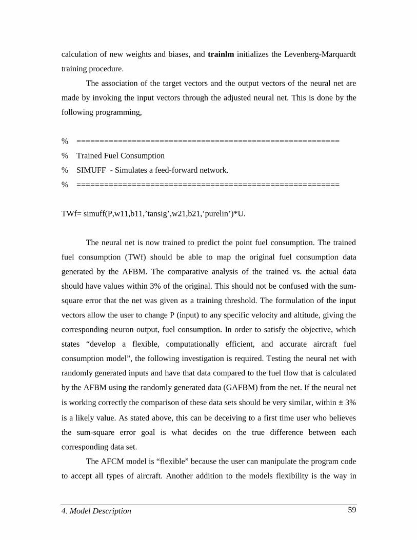
4. Model Description 59
calculation of new weights and biases, and trainlm initializes the Levenberg-Marquardt
training procedure.
The association of the target vectors and the output vectors of the neural net are
made by invoking the input vectors through the adjusted neural net. This is done by the
following programming,
% =========================================================
% Trained Fuel Consumption
% SIMUFF - Simulates a feed-forward network.
% =========================================================
TWf= simuff(P,w11,b11,’tansig’,w21,b21,’purelin’)*U.
The neural net is now trained to predict the point fuel consumption. The trained
fuel consumption (TWf) should be able to map the original fuel consumption data
generated by the AFBM. The comparative analysis of the trained vs. the actual data
should have values within 3% of the original. This should not be confused with the sum-
square error that the net was given as a training threshold. The formulation of the input
vectors allow the user to change P (input) to any specific velocity and altitude, giving the
corresponding neuron output, fuel consumption. In order to satisfy the objective, which
states “develop a flexible, computationally efficient, and accurate aircraft fuel
consumption model”, the following investigation is required. Testing the neural net with
randomly generated inputs and have that data compared to the fuel flow that is calculated
by the AFBM using the randomly generated data (GAFBM) from the net. If the neural net
is working correctly the comparison of these data sets should be very similar, within ± 3%
is a likely value. As stated above, this can be deceiving to a first time user who believes
the sum-square error goal is what decides on the true difference between each
corresponding data set.
The AFCM model is “flexible” because the user can manipulate the program code
to accept all types of aircraft. Another addition to the models flexibility is the way in
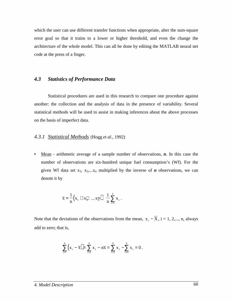
4. Model Description 60
which the user can use different transfer functions when appropriate, alter the sum-square
error goal so that it trains to a lower or higher threshold, and even the change the
architecture of the whole model. This can all be done by editing the MATLAB neural net
code at the press of a finger.
4.3 Statistics of Performance Data
Statistical procedures are used in this research to compare one procedure against
another: the collection and the analysis of data in the presence of variability. Several
statistical methods will be used to assist in making inferences about the above processes
on the basis of imperfect data.
4.3.1 Statistical Methods (Hogg et al., 1992)
• Mean - arithmetic average of a sample number of observations, n. In this case the
number of observations are six-hundred unique fuel consumption’s (Wf). For the
given Wf data set x1, x2,...xn multiplied by the inverse of n observations, we can
denote it by
( )xn
x x xn
xn ii
n
= + + ==∑1 1
1 21
... .
Note that the deviations of the observations from the mean, x Xi − , i = 1, 2,..., n, always
add to zero; that is,
( )x x x nx x xii
n
ii
n
ii
n
ii
n
− = − = − == = = =∑ ∑ ∑ ∑
1 1 1 1
0 .
4. Model Description 61
One can think of the mean as the fulcrum point that keeps a weightless ruler, on
which each observation is represented by the same weight, in perfect balance.
If we consider six-hundred Wf’s, then
x x ii
n
==∑1
600 1
For the complete set of six-hundred data points, the average or mean is xi. One
problem with the mean as the center of a data set is that it is effected by the presence of
one or several data points that lie very far to one side of the other values. This is called an
outlier. The AFCM was designed to eliminate these types of outliers by constraining the
velocity to certain altitudes. For example, FAA requires all commercial aircraft to travel
at speeds less then 250 knots when at an altitude of 10,000 feet or less. Applying this rule
to the program eliminated data that would normally not comply with the FAA rule. There
is still ambiguity within the data set in the high range, where an aircraft can fly at 200
knots with at an altitude of 45,000 feet: this is not realistic for level flight.
Measures of Variation
The standard deviation and variance are common measures of variability. The
sample variance and its square root, the standard deviation are measures of spread that are
based on normally distributed samples. The variance is the minimum variance unbiased
estimator of the normal parameter σ2. The standard deviation has the desirable property of
being in the same units as the data. That is, if the data is in lb/hr the standard deviation is
in lb/hr. The variance is in (lb/hr)2, which is more difficult to interpret. Neither the
standard deviation nor the variance is robust to outliers. A data value that is separate from
the body of the data can increase the value of the statistics by an arbitrarily large amount.
4. Model Description 62
• Variance-the square ( )x x− 2 of the distance x x− of an observation xi from the
overall average x provides some information about the variability, i = 1,2,..., n. The
variance is a special average of these n squared distances and is defined as
([ ) ( ) ( ] ( )sn
x x x x x xn
x xni
n2
1
2
2
2 2
2
2
1
1
1
1
1=
−− + − + + − =
−−
=∑... .
As stated above, it is the average of n such components, but we have divided the sum by
(n - 1) instead of n . This is because it was noted that the n deviations ( )x xi −2, i = 1,...,
n, add up to zero. Hence, we really need only (n - 1) of these deviations to calculate s2. It
is always possible to obtain the last deviation from
( ) ( )x x x xn ii
n
− = − −=
−
∑1
1
.
Therefore it seems justifiable to divide by n - 1 instead of n . The difference between the
two denominators make very little difference to large data sets (Schiff, 1996). An easier
way of calculating the variance that avoids working out the deviations from the mean is
( )s
nx
x x
nii
ni
n
2 2
1
2
2
11
1=
−−
−
=
=∑∑
.
• Standard Deviation-otherwise known as the Root Mean Square is simply the square
root of the variance. This method returns the original units of measurement and
denoted as
( )s sn
x xii
n
= =−
−=
∑2 2
1
1
1
4. Model Description 63
• t-test-is used in comparing two means, its purpose being to tell whether the means of
two sets of data are significantly different. The probability level corresponds to
computed t is the probability that the two means are truly different. In testing the
significance of means, the conventional procedure is to declare the difference
significant at the 95% probability level and highly significant at the 99% level. The t-
test consists of testing the truth of a hypothesis that two means are the same. This is
called the null hypothesis. The procedure is to calculate the probability of finding a
difference on the assumption that the null hypothesis is true. If the probability is
sufficiently small, the null hypothesis is rejected and we conclude that the two means
are truly different.
Conditions of the null hypothesis
Do not Reject if H0: µ1 = µ2 Reject if H1: µ1 ≠ µ2
For this test it will be assumed that the standard deviation, σ, is the same for both
means, because average fuel consumption was similar in both tests. The null hypothesis
to be tested is that the AFCM (X) and the AFBM (Y) are not significantly different. The
following method for calculating t was used in the research:
( )W S n t nw( ) ;≥ −α 1 .
This is called a paired-sample t-test where, W is the difference of each paired data
set (X, Y), Sw is the sample variance of the differences, and n is the number in the sample
set. The fuel consumption data was calculated on the basis that the input data set of the
AFBM (X) came from the AFCM (Y), and was expected to generate the same fuel
consumption’s. In this case the Xi and Yi are independent but expected to be related. In
such a situation we analyze the differences, Wi = Xi -Yi because these differences
“cancel” or adjust for subject differences that make measurements X and Y both appear
usually high or low. The differences W1 = X1 - Y1 , W2 = X2 - Y2 ,...Wn = Xn - Yn are

4. Model Description 64
then a random set of size n from a normal distribution with estimated population means
µ1 - µ2 and variance σ2W. The random variables W1 ,..., Wn are independent because they
are from observations on different sets of data. The distribution of W is normal, hence we
can use the t-test statistic. The summary of results for the aircraft set is depicted in Table
2.
4.4 Output of the Model
The output is the information provided by the AFCM. With the help of statistics
and graphics we can see how well the neural net trains and graphs the output of the
model. The output allows the user to make judgment on the data set and the functionality
of the model.
The individual models, AFBM and NNOM can be probed for information as well.
The AFBM is the bench mark for the entire research, without the output from this model
the AFCM would not exist. A t-test will be run for each pair of data that is generated by
these two models. If the results prove to be acceptable or we can accept the null
hypothesis then the models functionality is effective. All the statistical analysis is done in
MINITAB (Version 10Xtra, Minitab, Inc., 1995).
5. Model Application and Analysis 65
5. MODEL APPLICATION AND ANALYSIS
5.1 Introduction
This chapter presents the application of the developed AFCM. The model has
been tested with several different neural net architectures, two and three layer neural nets
accepting a range of input data that started at 225 randomly generated velocities and
altitudes. Each velocity had its own corresponding altitude. The AFBM used this data to
generate the fuel flow that was utilized as the target vector for the neural net. Other data
sets were tested, and it was decided to use 600 randomly generated sets. The results of
this research will contain graphical representation and statistical analysis of the data. A
Boeing 747-100, Boeing 767-200, Bombardier Dash-7, DC10-30 and Jetstar were used
for the performance calculations to show the strength and validity of the AFCM. The
Boeing 747-100 was used as the initial test aircraft for this research. It is widely known
around the world and can be termed “the power-house” of commercial aviation
transports. The aircraft, developed by Boeing in the mid-1960’ is primarily a trans-
oceanic aircraft. Its massive fuselage and fuel capacity can hold approximately 450
passengers traveling at stage lengths of nearly 5,000 miles. This is made possible by the
maximum take-off weight to fuel ratio of 3:1.
5.2 Model Application
The AFCM can be applied to future research in the aircraft fuel consumption
modeling arena. This research provides the “stepping stone” for future models that can
test any aircraft’s fuelburn under multiple variations of the airframe and the attitude at
which it flies. For example, an enhanced AFCM can handle multiple input variables such
as flap settings, gear position, weight change, and the attitude or position in which the
aircraft is flying: banking, G forces, etc.. The current model can produce fuel
5. Model Application and Analysis 66
consumption, thrust, velocity (both in Mach # and knots), altitude, and atmospheric
parameters at any point within the aircraft’s flight path.
5.3 Model Input Parameters
To demonstrate the versatility of the AFCM, the following data for each aircraft
can be manipulated. The Boeing 747-100 data is shown below and the rest of the aircraft
mix can be found in Appendix A.
Aircraft Characteristics
Aircraft B747-100 Engine JT9D-3A
VNE (not exceeding) = 517.00 knots VS = 110.00 knots
Operating Empty Weight
Maximum Takeoff Weight = 740,000 lb.
Number of Engines = 4 Wing Area = 5,500.00 ft2
AFBM Envelope: Velocity 200 knots - 300 knots (IAS)
Altitude Sea Level (0 ft) - 45,000 ft.
Random Generator: 600 data points between the above envelopes.
Altitude Sensitivity: Troposphere (0 - 36,089 ft.) & Stratosphere ( 36,089 - 45,000 ft.)
ρ = air density [lb/ft3]
σ = atmospheric density ratio
δ = pressure ratio
sv = sonic velocity [knots]

5. Model Application and Analysis 67
The AFCM calculates these parameters to simulate a dynamic atmospheric
environment. When calculating Mach number the above parameters are utilized to give
variations of speed as a function of altitude. The following MATLAB programming
calculates the Mach number:
M(i) = sqrt(5*[(r(i)*((1+0.2*[v(i)/661.5]^2)^3.5-1)+1)^0.286-1]),
where r is the inverse of the pressure ratio, δ, and v is the IAS. Figure 8 represents the
core equation constants that where extracted from SIMMOD, and found in the program
directory:
SIM\PROVER\PROGS\
Core Equation Constants for Boeing 747-100:
C(1) = 0.21105264 K(1) = 0.0151073814C(2) = 0.263755463 K(2) = -1.10763705E-06C(3) = -0.16161515 K(3) = 4.49822265E-08C(4) = 0.0758395116 K(4) = 0.0542092256C(5) = 0.0249066916 K(5) = -0.00853030039C(6) = -0.0253689568 K(6) = 0.00113895091C(7) = 0.149698643 K(7) = -6.32908055E-05C(8) = 0.493944407 K(8) = 1.28082643E-06C(9) = 0.0738636868 K(9) = -0.00092774075C(10) = -0.223604847 K(10) = 0.0195524624C(11) = -0.00700041482 K(11) = -0.00217159804C(12) = 0.0328436526 K(12) = 8.49267355E-05C(13) = 0.0435177226C(14) = 0.00514188666C(15) = 0.00134403024C(16) = 0.0306193895C(17) = 0.00983454066C(18) = -0.00845369234
FIGURE 8: Partial Aircraft Echo Report

5. Model Application and Analysis 68
The other core equation constants are also in Appendix A.
Change of Velocity Units: along with functions of fuel flow, thrust, lift coefficient and
drag coefficient, velocity units must be in feet/second rather then knots. The following
equation converts the velocity to ft/s by
V(i) = M(i)*sv(i)*1.6867,
where the product of Mach number and Sonic Velocity has units of knots that is
multiplied by the conversion factor of 1.6867 to give ft/sec.
The AFBM computes all the above to generate the fuel flow of that specific
aircraft. MATLAB allows the user to count floating point operations. The AFCM, as well
as the submodels have independent flop counters. Table 2 represents the results of the
models computational intensity [flops].
TABLE 2: Floating Point Operations
Model Function Technique No. of Layer’s No. ofNeuron’s
Flops
Per Network Per Layer
Energy
AFBM Balance Polynomial - - 89,600
AFCM2_6 TRAINLM LMBP 2 6 Rarely Converged
AFCM2_7 TRAINLM LMBP 2 7 56,400
AFCM2_8 TRAINLM LMBP 2 8 64,200
AFCM2_10 TRAINLM LMBP 2 10 79,800
AFCM3_6 TRAINLM LMBP 3 6 117,000
AFCM3_8 TRAINLM LMBP 3 8 125,800
5. Model Application and Analysis 69
Computationally, the AFCM has satisfied the objective by illustrating that the
AFCM2_7 was less computationally intensive. It was found that testing of various neural
net architectures the two-layer, seven-neuron model was 38% more efficient then Collins
path performance AFBM. Further results are still needed to totally satisfy the objective.
These will be presented in the next section.
5.4 Model Results
Now that the AFCM level of performance is determined, and proving its
performance to be faster then the AFBM, we can move on to the next portion of the
results that determine the functionality and accuracy of the model.
First, to insure that the AFBM is running correctly we can look at all the pertinent
output that reflects on the functionality of the model and most importantly the fuel
consumption profile of the model. This profile along with the velocity and altitude will be
the key part of the AFCM.
5.4.1 Graphical Analysis
Boeing 747-100 data will be used as for the graphical representation
FIGURE: 9
The plot of Velocity vs. Altitude illustrates the difference in velocity [TAS] as the
atmosphere changes. The profiles points are used as input vectors for the AFCM, initially
the AFBM utilizes the two variables to calculate fuel consumption. Once the fuel
consumption is calculated, inputs (velocity, altitude) and target vectors (fuel
consumption) funnel into the neural network.

5. Model Application and Analysis 70
FIGURE: 10
The graph illustrates the AFBM fuel consumption as a function of velocity and
altitude. The plot depicts the aircraft velocity and altitude limitations. For example the
Boeing 747-100 will travel at speeds of ±300 knots with a ceiling of 45,000 feet, where as
the Bombardier Dash-7 will not exceed 230 knots and 20,000 feet of altitude.
FIGURE: 11
The graph illustrates the drag vs Mach number and lift over drag vs Mach number.
What the first graph tells us is that drag increase as the aircraft’s speed increases. There is
a point in every profile where the drag is at the minimum. This is a good point to
recognize if fuel efficiency is to be maintained. The second graph shows that lift increases
relative to drag when speed is increased. As speed increases with altitude so does drag,
hence the ratio of lift over drag decreases.
FIGURE: 12
The plot of Ma vs Mach number, is observed to behave as profile drag. This value
generally constant until critical Mach is reached , after which there is an increase. Mb vs
Mach number, is observed to behave induced drag, where the value gradually decreases to
a minimum point which reflects the wing’s most efficient point, after which there is an
increase, and more of an increase as critical Mach becomes dominant. Mc vs Mach
number behaves much like the induced characteristics, there is a gradual increase until
critical Mach effects again cause rapid increase.
As we can see from these graphs, the drag rise associated with critical Mach has a large
impact on the shape of the curve.

5. Model Application and Analysis 71
FIGURE: 13
The first plot illustrates a comparison of fuel consumption’s between the trained
vs the generalized fuel consumption. Collins model generates the input needed by the
NNOM in order to train the weights and biases of the net that help produce the
association of input vectors to target vectors. After the network trains to a sum squared
error goal (SSEG) of 0.5%, the outputs will compare to the target vectors. Figure 16
represents the statistical results of the trained data to the actual data (Collins). It is
important not to associate the SSEG with the difference in the true means of the data set;
where the true means can be as large as 4% different. The second plot illustrates the
generalized neural net compared to the generalized AFBM (GAFBM).
FIGURE: 14
The plot of the AFCM vs GAFBM is observed to have a relative close
correspondence to one another. It tells us that the neural net is generalizing the data of the
trained net correctly by comparing it to the AFBM whose inputs are the generalized
random output of the AFCM. This tests both data sets for similarity of one another. The
next plot illustrates a histogram that represent the combination of the AFCM and
GAFBM data. The conclusion we can make from the histogram is that there is a relative
similarity between the data sets.
FIGURE: 15
The graph depicts a comparison of a specific input used in both the AFCM and AFBM. A
comparison of the fuel consumption output for the models are within 3% of each other.
Figures 9 - 15 denote the Boeing 747-100.
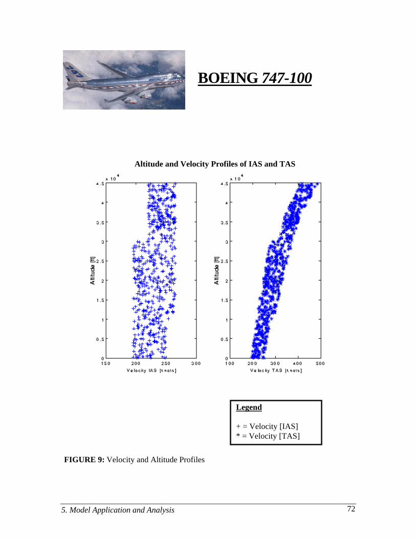
5. Model Application and Analysis 72
BOEING 747-100
FIGURE 9: Velocity and Altitude Profiles
Altitude and Velocity Profiles of IAS and TAS
Legend
+ = Velocity [IAS] * = Velocity [TAS]
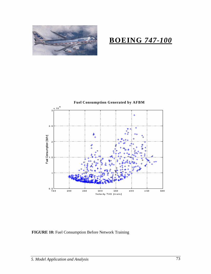
5. Model Application and Analysis 73
Fuel Consumption Generated by AFBM
BOEING 747-100
FIGURE 10: Fuel Consumption Before Network Training
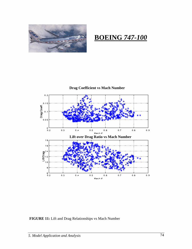
5. Model Application and Analysis 74
BOEING 747-100
Drag Coefficient vs Mach Number
Lift over Drag Ratio vs Mach Number
FIGURE 11: Lift and Drag Relationships vs Mach Number
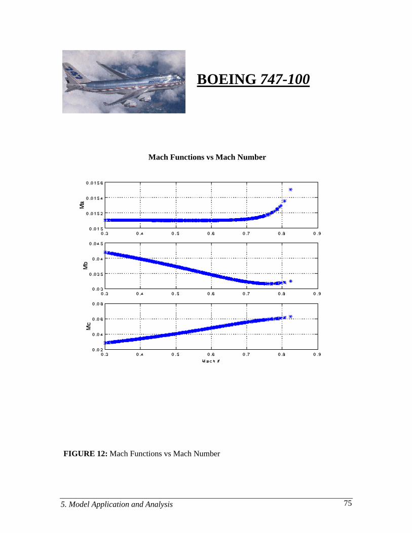
5. Model Application and Analysis 75
BOEING 747-100
Mach Functions vs Mach Number
FIGURE 12: Mach Functions vs Mach Number
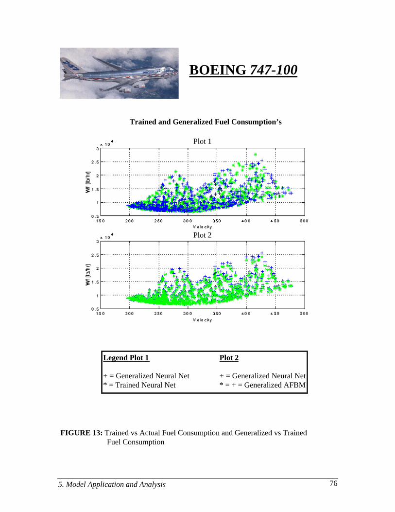
5. Model Application and Analysis 76
BOEING 747-100
Trained and Generalized Fuel Consumption’s
FIGURE 13: Trained vs Actual Fuel Consumption and Generalized vs TrainedFuel Consumption
Legend Plot 1 Plot 2
+ = Generalized Neural Net + = Generalized Neural Net* = Trained Neural Net * = + = Generalized AFBM
Plot 2
Plot 1
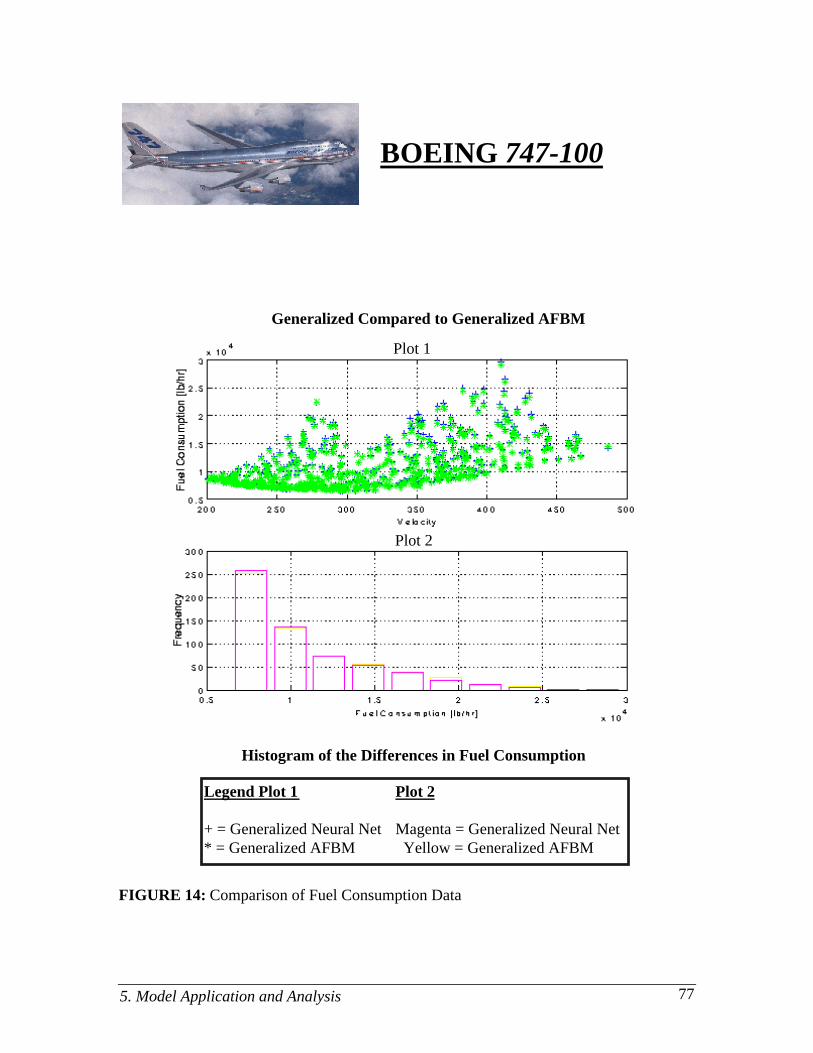
5. Model Application and Analysis 77
BOEING 747-100
Generalized Compared to Generalized AFBM
Histogram of the Differences in Fuel Consumption
FIGURE 14: Comparison of Fuel Consumption Data
Plot 1
Plot 2
Legend Plot 1 Plot 2
+ = Generalized Neural Net Magenta = Generalized Neural Net* = Generalized AFBM Yellow = Generalized AFBM
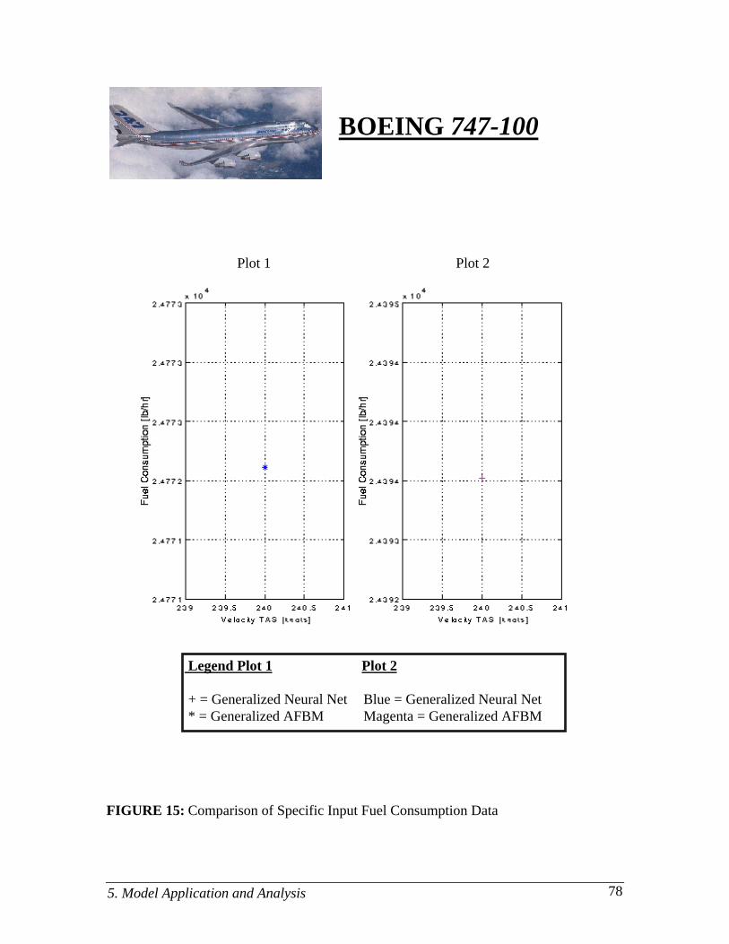
5. Model Application and Analysis 78
BOEING 747-100
Legend Plot 1 Plot 2
+ = Generalized Neural Net Blue = Generalized Neural Net * = Generalized AFBM Magenta = Generalized AFBM
FIGURE 15: Comparison of Specific Input Fuel Consumption Data
Plot 1 Plot 2
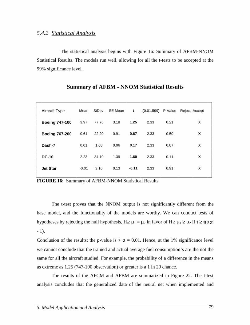
5. Model Application and Analysis 79
5.4.2 Statistical Analysis
The statistical analysis begins with Figure 16: Summary of AFBM-NNOM
Statistical Results. The models run well, allowing for all the t-tests to be accepted at the
99% significance level.
Summary of AFBM - NNOM Statistical Results
Aircraft Type Mean StDev. SE Mean t t(0.01,599) P-Value Reject Accept
Boeing 747-100 3.97 77.76 3.18 1.25 2.33 0.21 X
Boeing 767-200 0.61 22.20 0.91 0.67 2.33 0.50 X
Dash-7 0.01 1.68 0.06 0.17 2.33 0.87 X
DC-10 2.23 34.10 1.39 1.60 2.33 0.11 X
Jet Star -0.01 3.16 0.13 -0.11 2.33 0.91 X
FIGURE 16: Summary of AFBM-NNOM Statistical Results
The t-test proves that the NNOM output is not significantly different from the
base model, and the functionality of the models are worthy. We can conduct tests of
hypotheses by rejecting the null hypothesis, H0: µ1 = µ2 in favor of H1: µ1 ≥ µ2 if t ≥ t(α;n
- 1).
Conclusion of the results: the p-value is > α = 0.01. Hence, at the 1% significance level
we cannot conclude that the trained and actual average fuel consumption’s are the not the
same for all the aircraft studied. For example, the probability of a difference in the means
as extreme as 1.25 (747-100 observation) or greater is a 1 in 20 chance.
The results of the AFCM and AFBM are summarized in Figure 22. The t-test
analysis concludes that the generalized data of the neural net when implemented and
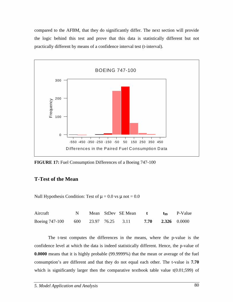
5. Model Application and Analysis 80
compared to the AFBM, that they do significantly differ. The next section will provide
the logic behind this test and prove that this data is statistically different but not
practically different by means of a confidence interval test (t-interval).
45035025015050-50-150-250-350-450-550
300
200
100
0
D ifferences in the Paired Fuel Consumption Data
Fre
quen
cy
BOEING 747-100
FIGURE 17: Fuel Consumption Differences of a Boeing 747-100
T-Test of the Mean
Null Hypothesis Condition: Test of µ = 0.0 vs µ not = 0.0
Aircraft N Mean StDev SE Mean t t99 P-Value
Boeing 747-100 600 23.97 76.25 3.11 7.70 2.326 0.0000
The t-test computes the differences in the means, where the p-value is the
confidence level at which the data is indeed statistically different. Hence, the p-value of
0.0000 means that it is highly probable (99.9999%) that the mean or average of the fuel
consumption’s are different and that they do not equal each other. The t-value is 7.70
which is significantly larger then the comparative textbook table value t(0.01;599) of

5. Model Application and Analysis 81
2.326. It is important to understand that this is a statistical difference, and not a practical
difference because there is ambiguity within the results. Figure 16 tells us that there is a
difference between the data sets but a relatively small difference when comparing each set
of fuel consumption data. In general, the most critical area of difference lies within the 50
lb/hr range. Also, the test states that the null hypothesis must be rejected because it does
not satisfy the mean conditionally: reject H0: mu1 = mu2 in favor of H1: mu1 ≠ mu2. It is
believed that the larger the sample set the more “power” it has to reject the null
hypothesis. This is because a large data set makes it more likely to contain several
different ranges of data and outliers. Hence, we can conclude that the means of each set
will have a better probability of not being equal to one another.
Confidence Intervals
Aircraft N Mean StDev SE Mean 99.0 % C.I.
Boeing 747-100 600 23.97 76.25 3.11 (15.93, 32.02)
The C.I. interval computes the hypothetical population mean difference of the
paired data set explaining how much the difference of each of these sets are on average.
This is a practical statistical approach where as the t-test only depicts statistical
information through the null hypothesis. The C.I. interval for this research computed a
99% confidence level that the true fuel consumption means lie within (15.93 lb/hr, 32.02
lb/hr). Using this test proves that the initial assumption is correct: the data sets are
closely related. At this point a statistician can not conclude that the C.I. results are within
a tolerable fuel consumption range. This is an engineers decision on whether or not the
above range is acceptable. The outcome for the results are as follows:
♦ 99% of the time the model will produce a true average difference of fuel consumption
that lies within a tolerable range.
♦ The results are reasonable because 15.93 lb/hr - 32.02 lb/hr range is considered
negligible when assuming an aircraft of this stature burns a minimum of 30,000 lb/hr.

5. Model Application and Analysis 82
Figures 18-21 will denote the fuel consumption differences and statistical analysis
for the rest of the aircraft mix used in this research.
500 lb/hr400 lb/hr300 lb/hr200 lb/hr100 lb/hr0 lb/hr-100 lb/hr
300
200
100
0
Differences in the Paired Fuel Consumption Data
Fre
que
ncy
Boeing 767-200
FIGURE 18: Fuel Consumption Differences of a Boeing 767-200
T-Test of the Mean
Null Hypothesis Condition: Test of µ = 0.0 vs µ not = 0.0
Aircraft N Mean StDev SE Mean t t99 P-Value
Boeing 767-200 600 0.95 37.79 1.54 0.63 2.326 0.5400
Confidence Intervals
Aircraft N Mean StDev SE Mean 99.0 % C.I.
Boeing 767-200 600 0.95 37.79 1.64 (4.9, 13.3)
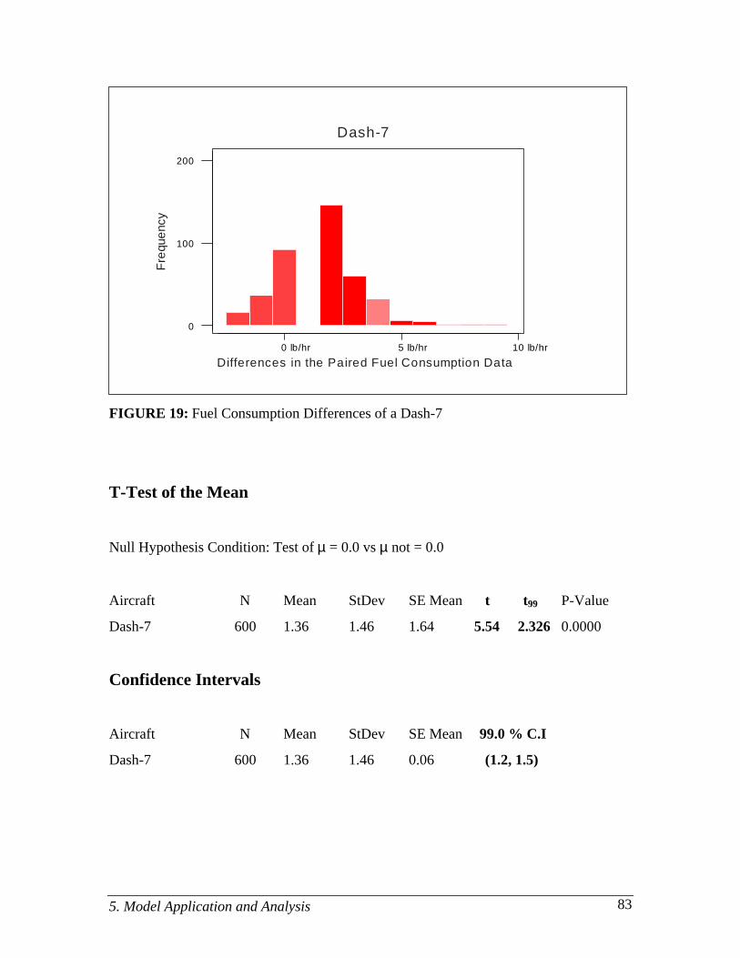
5. Model Application and Analysis 83
10 lb/hr5 lb/hr0 lb/hr
200
100
0
Differences in the Paired Fuel Consumption Data
Fre
quen
cy
Dash-7
FIGURE 19: Fuel Consumption Differences of a Dash-7
T-Test of the Mean
Null Hypothesis Condition: Test of µ = 0.0 vs µ not = 0.0
Aircraft N Mean StDev SE Mean t t99 P-Value
Dash-7 600 1.36 1.46 1.64 5.54 2.326 0.0000
Confidence Intervals
Aircraft N Mean StDev SE Mean 99.0 % C.I
Dash-7 600 1.36 1.46 0.06 (1.2, 1.5)

5. Model Application and Analysis 84
400 lb/hr200 lb/hr0 lb/hr-200 lb/hr-400 lb/hr
150
100
50
0
D ifferences in the Paired Fuel Consumption Data
Fre
que
ncy
McDonnell-Douglas DC10-30
FIGURE 20: Fuel Consumption Differences of a DC10-30
T-Test of the Mean
Null Hypothesis Condition: Test of µ = 0.0 vs µ not = 0.0
Aircraft N Mean StDev SE Mean t t99 P-Value
DC10-30 600 32.80 58.70 2.40 13.71 2.326 0.0000
Confidence Intervals
Aircraft N Mean StDev SE Mean 99.0 % C.I.
DC10-30 600 32.80 58.70 2.40 (26.7, 39.1)
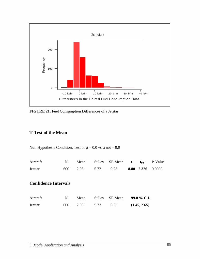
5. Model Application and Analysis 85
40 lb/hr30 lb/hr20 lb/hr10 lb/hr0 lb/hr-10 lb/hr
200
100
0
Differences in the Paired Fuel Consumption Data
Fre
que
ncy
Jetstar
FIGURE 21: Fuel Consumption Differences of a Jetstar
T-Test of the Mean
Null Hypothesis Condition: Test of µ = 0.0 vs µ not = 0.0
Aircraft N Mean StDev SE Mean t t99 P-Value
Jetstar 600 2.05 5.72 0.23 8.80 2.326 0.0000
Confidence Intervals
Aircraft N Mean StDev SE Mean 99.0 % C.I.
Jetstar 600 2.05 5.72 0.23 (1.45, 2.65)
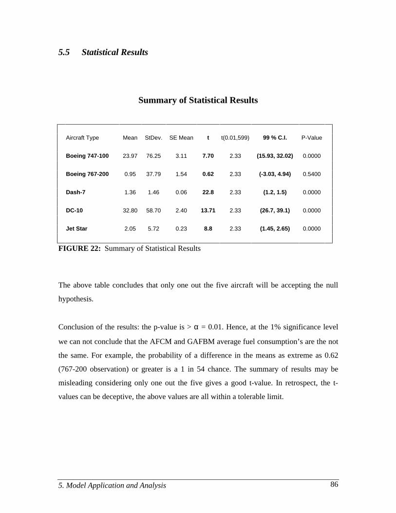
5. Model Application and Analysis 86
5.5 Statistical Results
Summary of Statistical Results
Aircraft Type Mean StDev. SE Mean t t(0.01,599) 99 % C.I. P-Value
Boeing 747-100 23.97 76.25 3.11 7.70 2.33 (15.93, 32.02) 0.0000
Boeing 767-200 0.95 37.79 1.54 0.62 2.33 (-3.03, 4.94) 0.5400
Dash-7 1.36 1.46 0.06 22.8 2.33 (1.2, 1.5) 0.0000
DC-10 32.80 58.70 2.40 13.71 2.33 (26.7, 39.1) 0.0000
Jet Star 2.05 5.72 0.23 8.8 2.33 (1.45, 2.65) 0.0000
FIGURE 22: Summary of Statistical Results
The above table concludes that only one out the five aircraft will be accepting the null
hypothesis.
Conclusion of the results: the p-value is > α = 0.01. Hence, at the 1% significance level
we can not conclude that the AFCM and GAFBM average fuel consumption’s are the not
the same. For example, the probability of a difference in the means as extreme as 0.62
(767-200 observation) or greater is a 1 in 54 chance. The summary of results may be
misleading considering only one out the five gives a good t-value. In retrospect, the t-
values can be deceptive, the above values are all within a tolerable limit.
6. Conclusions and Recommendations 87
6. CONCLUSIONS AND RECOMMENDATIONS
6.1 Introduction
This final chapter describes issues underlying the development of the AFCM and
the use of the MATLAB Neural Network software. The recommendations are made to
improve the accuracy and enhancement of the Aircraft Fuel Consumption Model.
6.2 Conclusions
The AFCM developed through this research has been designed to provide air
transportation designers the information and foundation needed to encompass an accurate
working fuel consumption model into a landside/airside model such as SIMMOD. The
objective of this research; to utilize a modeling simulation software to develop a flexible,
computationally efficient, and accurate aircraft fuel consumption model, has been
accomplished. The energy balance concept in combination with a neural network was
successfully developed and applied to modeling aircraft energy performance. The energy
balance algorithm accepts as inputs aircraft specific limitations, such as velocity, altitude,
and weight. Other equations compensate for altitude change giving both minimum and
maximum conditions. When the performance data is generated it directly goes into the
neural net as input vectors and target vectors. Two inputs containing 600 randomly
generated pieces of data flow feedforward and then are backpropagated until the net
reaches its sum-square error goal. These inputs have a direct relation with the target
vectors. This relation or association is what makes the neural net so powerful. Once the
net has trained it can handle any input with a finite amount of discontinuities and deliver
accurate output that is comparable to the AFBM. The beauty about the neural net is that it
learns through optimization how to generalized input at a fraction of the computational
expense relative to other programs that do the same tasks. Computationally, the AFCM

6. Conclusions and Recommendations 88
has satisfied the objective by illustrating that it was indeed less computationally intensive.
It was found that through testing various neural net architectures the two-layer, seven-
neuron model was 38% more efficient then Collins path performance AFBM and remain
just as accurate.
The level of computational effort of this model could be viewed as “low level”
because of the absence of input variables. Typically a fuel consumption model would
incorporate many variables. The two input variables, velocity and altitude satisfy the
present research and give light to future model’s that could incorporate many input
variables. By using the aircraft’s total energy as point performance rather then path
performance the AFCM is an efficient model for computing point performance for a
multiple range of aircraft. The computational efficiency makes it attractive for parametric
studies as well as enhancement.
It was verified statistically that the AFCM was competent in computing fuel
consumption as a point performance model. The trained data set was within ±3% of the
actual data, and the generalized data set was within ±4% of the generalized AFBM.
In conclusion, this model is practical for modeling fuel consumption. The
SIMMOD fuelburn post-processor utilizes the energy balance concept but lacks in the
versatility and thrives on computational expense. At the present time, AVERAGE
ERROR - Over the entire three dimensional state, we sample any data point on the
average and approximately get ±4% discrepancy of fuel flow. Where as SIMMOD has a
high discrepancy within some of its aircraft mix. For example, if a commercial aviation
company such as USAir would like to find out how much their F-28 aircraft uses via
SIMMOD, the fuel coefficients for that aircraft are of a DC-9 giving a 25% inaccuracy.
This discrepancy is extremely high and this is the reason USAir would never utilize
SIMMOD for estimating fuel consumption.
• If a substitution is given for an undefined aircraft which delivers 25%
inaccuracies, then why use the fuelburn post-processor in the first place? The fuel
burn post processor will hinder the confidence of the outputs. Therefore, redefine
the entire aircraft mix to achieve a high level of confidence in the output.
6. Conclusions and Recommendations 89
Arguments: If it is tolerable for SIMMOD to have 4% maximum difference between
calculated and published values and 1.4% average error, then it is better to apply the
tolerable errors to the entire aircraft mix instead of having 17 aircraft in the mix defined
while 90 remain undefined. The AFCM can be implemented to take over for the AFBM
with near accurate values. In one case the 3% - 4% difference of the AFCM to the AFBM
could be the exact value of the published data that Collins based his error differences on.
In addition to the AFCM’s use for determining point performance of an aircraft it
can be easily used as a dynamic path profile model as well. In order to do so the user can
take point performance at two different points within the profile, integrate over that
distance with respect to time, and generate path like performance. The next section will
be the recommendations to this research.
6.3 Recommendations
The goal of the recommendations are to provide the reader with the sort comings
of the model and positive insight to a future model. A highly significant recommendation
would be to try this model with multiple inputs such as flap settings, landing gear, and
more atmospheric conditions such as head wind. The AFCM is a quasi-steady state model
where time has no inference, it would be desirable for the model to become path
performance oriented. Also to be able to incorporate banking forces and or gravitational
forces under implications that fuel consumption changes drastically with these conditions.
One of the concerns in this research is the way Collins derived the core
coefficients. These coefficients are aircraft specific, the question is how they were
generated. Considering that the drag coefficient plays a major role in the energy balance
equation, it is to my understanding that there are several ways of determining drag
coefficients. Another recommendation would be to identify a more precise way in
determining drag coefficients or use a three-way methodology where the modeller can
take an average of three techniques used in determining drag forces. The following
methodology could apply:
6. Conclusions and Recommendations 90
♦ Use of aeronautical calculations: finding drag coefficients through empirical
formulation.
♦ Wind tunnel tests, using an aircraft model.
♦ Actual full scale aircraft testing.
Typically the above processes are nothing new but if we can refine the way in
which this data is collected and take the average values of the three techniques we could
better each aircraft specific constants. The question now is
♦ How does the empirical formulation compare to the wind tunnel testing?
♦ Does the output have a small margin of error?
♦ How does the empirical formulation compare to the actual aircraft’s data?
♦ Do any of the above coincide with one another having a minimum margin of error?
One of the other important factors to expose is that drag coefficients do not have a
direct correlation with the internal workings that exist within a turbo jet engine. It is
recommended to gather internal engine performance data to see if there is any validity in
this concept. To do so, the following is recommended:
♦ Gather historical data from engine tests at both airline and engine overhaul shops.
♦ Obtain airline in-flight recordings
These are the main recommendations as a result of the exposure and experience
gained in developing the AFCM. I further believe these are valid points to test and apply
to a future AFCM.

Bibliography 91
BIBLIOGRAPHY
1. “Aircraft Data.” Federal Aviation Administration Advisory Circular 150/5325-5C.
FAA, 1987.
2. Antsaklis, P.J., and Moody, J.O. “The Dependence Identification Neural
Network Construction Algorithm.” IEEE Transactions on Neural Networks, Vol.
7, No.1, January 1996, pp. 3-15.
3. Baran, Robert H. and Coughlin, James P. “Neural Computation in Hopfield
Networks and Boltzmann Machines.” Newark: University of Delaware Press,
1994.
4. Barbeau, E.J. “Polynomials.” New York: Springer-Verlag, 1989.
5. Beal, Mark. and Demuth, Howard. “Training Functions in a Neural Network
Design Tool.” In Proceedings of the Third Workshop on Neural Networks
Academic/ Industrial/ NASA/ Defense ’92. SPIE Vol. 1721, 1992.
6. Burrows, James W. “Fuel Optimal Trajectory Computation.” Boeing Computer
Services Company. Seattle, Wash. AIAA 82-4084, Vol. 19, No.4, April 1982.
7. Collins, B.P., Bell, Noel. J., and Ford, David. W. “Concepts for Aviation Fuel
Efficiency.” Aviation Fuel Consumption Symposium, September 10-11, 1984.
8. Collins, B.P. “Derivation and Current Capabilities of the Path Profile Fuel
Consumption Algorithm.” The MITRE Corporation. McLean, VA. MTR-
80W195, September 1980a.
9. Collins, B.P. “Estimation of Fuel Consumption of Commercial Jet Aircraft from
Path Profile Data.” The MITRE Corporation. McLean, VA. MP-80W7, May
1980b.
10. Collins, B.P. “Estimation of Turbojet Fuel Consumption from Tracking Data.”
The MITRE Corporation. McLean, VA. MTR-79W344, September 1979.
11. Ecker, Joseph G. and Kupferschmid, Michael. “Introduction to Operations
Research.” New York: John Wiley & Sons, 1988.

Bibliography 92
12. Ethell, Jeffrey L. “Fuel Economy in Aviation.” NASA SP-462, Washington, DC.,
1983.
13. Etter, D.M. “Engineering Problem Solving with MATLAB.” NJ: Prentice Hall,
Englewood Cliffs, 1993.
14. Gosselin, C.M., Le-Huy, H., and Payeur, P. “Trajectory Prediction for
Moving Objects Using Artificial Neural Networks.” IEEE Transactions on
Industrial Electronics. Vol. 42, No.2, April 1995, pp. 147-158.
15. Grossberg, S., ‘Competitive Learning From Interactive Activation to Adaptive
Resonance.” Cognitive Science, 11, 23-63.
16. Hagan, M., Demuth, H., Beal, M., “Neural Network Design.” New York: Thomas
Publishing Co., 1996.
17. Hogg, Robert. V., Ledolter, Johannes. “Applied Statistics for Engineers and
Physical Scientists.” New York, Macmillian Publishing Company, 2ed., 1992.
18. Khanna, T. “Foundations of Neural Networks.” New York: Addison-Wesley, 1990.
19. Lau, C., “Neural Networks: theoretical foundation and analysis.” New York: IEEE
Press, 1992.
20. Mair, Austyn. W., and Birdsall, David. L., “Aircraft Performance.” Cambridge
Aerospace Series 5. New York: Cambridge University Press. 1992.
21. Maren, Alianna J. “A Logical Topology of Neural Networks.” In Proceedings
of the Third Workshop on Neural Networks - Academic/ Industrial/ NASA/
Defense ’92. SPIE Vol. 1515, 1991.
22. MATLAB 4.0 . The Math Works Inc., 1992.
23. McCormick, Barnes W. “Aerodynamics, Aeronautics and Flight Mechanics.” New
York, London: John Wiley & Sons, 1995.
24. MINITAB 10Xtra . Minitab Inc., 1995.
25. Murphy, John H. “Neural Network Learning Algorithms.” In Proceedings of the
Third Workshop on Neural Networks - Academic/ Industrial/ NASA/
Defense ’91. SPIE Vol. 1515. 1991.
26. Neural Network TOOLBOX 2.0 . The Math Works Inc., 1994.

Bibliography 93
27. Ripley, Brian D. “Networks and Chaos: Statistical and Probabilistic Aspects.” eds.
O.E. Barndorff-Nielsen, J.L. Jensen, and W.S. Kendall. London: Chapman &
Hall, 1993.
28. Roskam, J. “Airplane Design: Part I, Preliminary Sizing of Airplanes.”
Roskam Aviation and Engineering Corporation. Kansas: Ottawa, 1989a.
29. Roskam, J. “Airplane Design: Part II, Preliminary Configuration Design and
Integration of The Propulsion System.” Roskam Aviation and Engineering
Corporation. Kansas: Ottawa, 1989b.
30. Roskam, J. “Airplane Design: Part VI, Preliminary Calculation of Aerodynamic,
Thrust and Power Characteristics.” Roskam Aviation and Engineering
Corporation. Kansas: Ottawa, 1989c.
31. Ruijgrok, G.J.J. “Elements of Airplane Performance.” Netherlands: Delft
University Press, 1990. pp. 136-157.
32. Rumelhart, D.E., Hinton, G.E., Williams, R.J., “Parallel Distributed Processing:
Learning Internal Representations by Error Propagation,” Vol. 2. Cambridge MA:
The MIT Press.
33. Saltz, D., “A Short Calculus: an applied approach.” California: Goodyear
Publishing Co. 1974.
34. Scales, L.E., “Introduction to NON-Linear Optimization.” New York: Springer-
Verlag, 1985.
35. Schiff, Daniel., D’Agostino, Ralph. B., “Practical Engineering Statistics.” New
York, John Wiley & Sons, Inc., 1996.
36. “SIMMOD User’s Manual.” CACI Products Company. Arlington, VA., 1989a.
37. “SIMMOD Reference Manual.” CACI Products Company. Arlington, VA., 1989b.
38. “SIMMOD Data Input Manual.” CACI Products Company. Arlington, VA., 1989c.
39. United States Standard Atmosphere; 1962: Geopotential Altitude.
40. United States. House of Representatives. Committee on Science. Subcommittee on
Technology. Federal Aviation Admin. Research and Organizational Management.
104 Congress, first session. May 16, 1995.

Bibliography 94
41. Vinh, Nguyen. X., “Aircraft Performance.” Cambridge Aerospace Series 4. New
York: Cambridge University Press. 1993.
42. Widrow, B., and M.E. Hoff. 1960. “Adaptive Switching Circuits.” IRE WESCON
Convention Record 4:96-104.

Appendix A 95
Aircraft Core Coefficients
%Aircraft B747-100%Engines JT9D-3A%VNE 517[knots]%VS 110[knots]%Idle Fuel Consumption 800[lb/hr]%MTOW 733000[lb]%EW 400000[lb]%Number of Engines 4%Wing Area 5500[ft^2]
Core Equations
.21105264
.263755463-.16161515.0758395116.0249066916-.0253689568.149698643.493944407.0738636868-.223604847-7.00041482E-03.0328436526.04351772265.14188666E-031.34403024E-03.03061938959.83454066E-03-8.45369234E-03.0151073814-1.10763705E-064.49822265E-08.0542092256-8.53030039E-031.13895091E-03-6.32908055E-051.28082643E-06-9.2774075E-04
.0195524624-2.17159804E-038.49267355E-0555004733000
APPENDIX A

Appendix A 96
Aircraft Core Coefficients
%Aircraft B767-200%Engines CF6-80A%VNE 518[knots]%VS 119[knots]%Idle Fuel Consumption 550[lb/hr]%MTOW 300000.[lb]%EW 175300[lb]%Number of Engines 2%Wing Area 3050[ft^2]
Core Equations
.0368209248
.369535404-.07946150571.19172123E-03.0126832447-9.64166545E-03.220878642.637665565.076206901-.291661654-4.33010235E-03.0285686323.0332591028-.0818162599-3.73336704E-03.0382619471-1.93000345E-037.39639837E-03200325045000.01215991032.81166465E-054.38357117E-08.03199862819.8614769E-03-1.71543457E-03
5.88580465E-051.01565402E-061.65178004E-034.11909335E-03-1.58661376E-032.45352206E-0430502300000

Appendix A 97
Aircraft Core Coefficients
%Aircraft DASH-7%Engines PT6A-50%VNE 231[knots]%VS 100[knots]%Idle Fuel Consumption 150[lb/hr]%MTOW 44000[lb]%EW 27600[lb]%Number of Engines 2%Wing Area 860[ft^2]
Core Equations
.0378468694-.0397568785-6.11851844E-03-7.30640239E-045.69681434E-03-.0181243268-1.200895626.02542599-.0523632417-.482001873-.231751712.9611041627.25989187-35.3552068-1.033621638.45154993.20630902-13.0177043150230020000.0357470547-8.4236005E-038.99588121E-04.715305576-1.422529.703446842-5.36434698E-03
-.03963631741.180382871.12145574-1.93252476.541605849860.02.44000.

Appendix A 98
Aircraft Core Coefficients
%Aircraft DC10-30%Engines CF6-50A%VNE 530[knots]%VS 106[knots]%Idle Fuel Consumption 550[lb/hr]%MTOW 565000[lb]%EW 118860[lb]%Number of Engines 3%Wing Area 3958[ft^2]
Core Coefficients
.0969402237
.226048248-.0360260455-.07064694683.25553256E-036.93085303E-03.176102017.688138063.0243108193-.1249429061.00018273E-039.17626224E-03.0493856238-.07558156786.91019055E-034.82393939E-03-1.40794519E-031.81113083E-03200300045000.01550815381.97064056E-05-3.715255E-09.04317484772.08393033E-034.49095588E-04-1.26675922E-04
5.43086401E-06 .0276335295-5.60263473E-03-8.20214212E-04 1.76284875E-043958.3.565000.

Appendix A 99
Aircraft Core Coefficients
%Aircraft JETSTAR%Engines TFE731-3%VNE 505[knots]%VS 92[knots]%Idle Fuel Consumption 100[lb/hr]%MTOW 42000[lb]%EW 26000[lb]%Number of Engines 4%Wing Area 542.5[ft^2]
Core Equations
.0134841031
.0303350088-4.51805667E-03-3.79565448E-033.52973105E-048.16723206E-05.365299873.656439584.0266137971-.251847417-6.88010077E-03.0317623623.406080785-.867605946-.26626554.852064046.113603167-.109188801190280045000.0246452545-2.44355304E-042.74194508E-06-.149335028.0919067503-.0144818473
1.21881272E-03-4.12300952E-05.639278364-.246838727.0320710432-1.38999953E-03542.5442000

Appendix B 100
APPENDIX B
Aircraft Fuel Consumption Model Program
%*************************A F C M 2 7 BOEING 747-100*******************
% Title :FUEL CONSUMPTION MODEL% Author :Glenn D. Schilling
%FUEL BURN MODEL CORE EQUATION
% Velocity and Altitude Iputs
Vlow = 195;, Vhigh = 265;, Hlow = 0;, Hhigh = 45000;
pts = 600; % Number of random pointsR = rand(pts,2); % Random Generatorfor i=1:1:pts;
v(i) = Vlow + (Vhigh-Vlow)*R(i,1);A(i) = Hlow + (Hhigh-Hlow)*R(i,2);h(i) = A(i)*0.0001;
if A(i) <= 10000v(i) = Vlow + (250-Vlow)*R(i,1);
elseif A(i) > 30000v(i) = 220 + (240-Vlow)*R(i,1);end
% Air Density and ICAO Standard Atmosphere
if A(i) <= 36089rho(i) = 0.0023769*[1-6.88*10^(-6)*(A(i))]^4.2563; % Air Densitysv(i) = 661.5 - [((661.5 - 573.6)/360 89)*A(i)]; % Sonic Velocity
elseif A(i) > 36089rho(i) = 0.00070627*exp((36089-A(i))/20806.6);sv(i) = 573.6;,endsig(i) = rho(i)/0.0023769; % Atmoshperic Density Ratior(i) = 1/sig(i);
% Mach Number
M(i) = sqrt(5*[(r(i)*((1+0.2*[v(i)/661.5]^2)^3.5-1)+1)^0.286-1]);
RHO(i) = (1+M(i))/(1-M(i)); %Mach Number Ratio
% Velocity Calibration [ TAS, ft/sec ]
V(i) = M(i)*sv(i)*1.6867;Vkts(i) = M(i)*sv(i);
O = max(max(Vkts));% Normalize Function
% Fuel Flow Constants
format longfid = fopen(’b747.dat’);c = fscanf(fid,’%g’,[33]);

Appendix B 101
fclose(fid);C1=c(1);,C2=c(2);,C3=c(3);,C4=c(4);,C5=c(5);,C6=c(6);,C7=c(7);C8=c(8);,C9=c(9);,C10=c(10);,C11=c(11);,C12=c(12);,C13=c(13);C14=c(14);,C15=c(15);,C16=c(16);,C17=c(17);,C18=c(18);,K1=c(19);K2=c(20);,K3=c(21);,K4=c(22);,K5=c(23);,K6=c(24);,K7=c(25);K8=c(26);,K9=c(27);,K10=c(28);,K11=c(29);,K12=c(30);,Sw=c(31);N=c(32);,W=c(33);
% Functions of Fuel Flow
F1(i)=C1+C2*M(i)+C3*h(i)+C4*M(i)*h(i)+C5*h(i)^2+C6*M(i)*h(i)^2;F2(i)=[C7+C8*M(i)+C9*h(i)+C10*M(i)*h(i)+C11*h(i)^2+C12*M(i)*h(i)^2]*(N*10^4)^(-1);F3(i)=[C13+C14*M(i)+C15*h(i)+C16*M(i)*h(i)+C17*h(i)^2+C18*M(i)*h(i)^2]*(N*10^4)^(-2);
% Functions of Mach Number
Ma(i) = K1+K2*RHO(i)^2+K3*RHO(i)^4;Mb(i) = K4+K5*RHO(i)+K6*RHO(i)^2+K7*RHO(i)^3+K8*RHO(i)^4;Mc(i) = K9+K10*RHO(i)+K11*RHO(i)^2+K12*RHO(i)^3;
% Total Drag Coefficient
Cd(i)=Ma(i)+Mb(i)*(W/(0.5*rho(i)*Sw*V(i)^2))^2+Mc(i)*(W/(0.5*rho(i)*Sw*V(i)^2))^4;
% Thrust Coefficient
Thrust(i) = 0.5*rho(i)*Sw*V(i)^2*Cd(i);
format short% Fuel Flow per Engine (lb/hr)
Wf(i) = [F1(i)+F2(i)*Thrust(i)+F3(i)*Thrust(i)^2]*10000;
% Lift over Drag Ratio
Cl(i) = W/(0.5*rho(i)*Sw*V(i)^2);LD_Ratio(i) = Cl(i)/Cd(i);
end
U = max(max(Wf));% Normalize Function
%Plot Speeed vs. Velocity
subplot (1,2,1);plot (v,A,’+’);title(’VELOCITY - ALTITUDE PROFILE’);xlabel(’Velocity IAS [knots]’);ylabel(’Altitude [ft]’);subplot (1,2,2);plot (Vkts,A,’*’);title(’VELOCITY - ALTITUDE PROFILE’);xlabel(’Velocity TAS [knots]’);ylabel(’Altitude [ft]’);save va1747pauseclfplot(Vkts,Wf,’+’);title(’AFBM’);xlabel(’Velocity TAS [knots]’);ylabel(’Fuel Consumption [lb/hr]’);

Appendix B 102
gridsave afbm747.ps%*************************************************************% Function approximation with Levenberg-Marquardt.% Envoke the Neural Network% The function of the neural network learns as it passes% through these data points.%*************************************************************
% Data Points (Input and Target Vectors)
P = [Vkts/O;A/45000;];% InputT1 = Wf/U;% Target
S1 = 7;% Number of hidden neurons in the first layer
df = 10; % Frequency of progress displays (in epochs).me = 1000; % Maximum number of epochs to train.eg = 0.005; % Sum-squared error goal.tp = [df me eg];
%*************************************************************% INITFF is used to initialize the weights and biases for% the Two Layer (TANSIG/PURELIN) network.%*************************************************************
[w11,b11,w21,b21] = initff(P,S1,’tansig’,T1,’purelin’);%Initialize% Weights and Biases
%*************************************************************% TRAINLM - Trains a feed-forward network with faster bckprp.%*************************************************************
% Training the Neural with a Levenberg-Marquardt Backpropagation Algorithm
[w11,b11,w21,b21,ep,tr]=trainlm(w11,b11,’tansig’,w21,b21,’purelin’,P,T1,tp);
save sseb747.ps%*************************************************************% SIMUFF - Simulates a feed-forward network.%*************************************************************% Trained Fuel Consumptionflops(0);TWf= simuff(P,w11,b11,’tansig’,w21,b21,’purelin’)*U;flopsX = Wf’;Y = TWf’;Z = [X Y];plot(Vkts,Wf,’*’,Vkts,TWf,’+’);title(’AFBM vs TRAINED FUEL CONS.’);xlabel(’Velocity TAS [knots]’)ylabel(’Fuel Consumption {lb/hr]’)gridsave tvsafbm747.pssave twf747.dat Z -ascii
%*************************************************************% USING THE PATTERN ASSOCIATOR%*************************************************************vlow = 195;, vhigh = 265;, hlow = 0;, hhigh = 45000;

Appendix B 103
points = 600;% Number of random pointsr = rand(points,2);% Random Generatorfor i=1:1:pts;
vel(i) = vlow + (vhigh-vlow)*r(i,1);alt(i) = hlow + (hhigh-hlow)*r(i,2);h1(i) = alt(i)*0.0001;
if alt(i) <= 10000vel(i) = vlow + (250-vlow)*r(i,1);
elseif alt(i) > 30000 vel(i) = 220 + (240-vlow)*r(i,1);
end
if alt(i) <= 36089Rho(i) = 0.0023769*[1-6.88*10^(-6)*(alt(i))]^4.2563; % Air DensitySv(i) = 661.5 - [((661.5 - 573.6)/36089)*alt(i)];% Sonic Velocity
elseif alt(i) > 36089Rho(i) = 0.00070627*exp((36089-alt(i))/20806.6);% Air DensitySv(i) = 573.6;% Sonic VelocityendSig(i) = Rho(i)/0.0023769; % Atmoshperic Density RatioDr(i) = 1/Sig(i);
% Mach Number
Mn(i)=sqrt(5*[(Dr(i)*((1+0.2*[vel(i)/661.5]^2)^3.5-1)+1)^0.286-1]);
mnr(i) = (1+Mn(i))/(1-Mn(i)); %Mach Number Ratio
% Sonic Velocity [ TAS, ft/sec ]
Vfs(i) = Mn(i)*Sv(i)*1.6867;Vknots(i) = Mn(i)*Sv(i);
%*************************************************************% Neural Generalized Data can be Implemented back to% the Original Base Fuel Consumption Algorithm% to test the accuracy of Neural Nets Generalization% and to see if the inputs (Velocity and Altitude)and% targets fit within a marginal error.%*************************************************************
% Functions of Fuel Flow
F11(i)=C1+C2*Mn(i)+C3*h1(i)+C4*Mn(i)*h1(i)+C5*h1(i)^2+C6*Mn(i)*h1(i)^2;F21(i)=[C7+C8*Mn(i)+C9*h1(i)+C10*Mn(i)*h1(i)+C11*h1(i)^2+C12*Mn(i)*h1(i)^2]*(N*10^4)^(-1);F31(i)=[C13+C14*Mn(i)+C15*h1(i)+C16*Mn(i)*h1(i)+C17*h1(i)^2+C18*Mn(i)*h1(i)^2]*(N*10^4)^(-2);
% Functions of Mach Number
Ma1(i) = K1+K2*mnr(i)^2+K3*mnr(i)^4;Mb1(i) = K4+K5*mnr(i)+K6*mnr(i)^2+K7*mnr(i)^3+K8*mnr(i)^4;Mc1(i) = K9+K10*mnr(i)+K11*mnr(i)^2+K12*mnr(i)^3;
% Total Drag Coefficient
Cd1(i)=Ma1(i)+Mb1(i)*(W/(0.5*Rho(i)*Sw*Vfs(i)^2))^2+Mc1(i)*(W/(0.5*Rho(i)*Sw*Vfs(i)^2))^4;

Appendix B 104
% Thrust Coefficient (lb)
Thrust1(i) = 0.5*Rho(i)*Sw*Vfs(i)^2*Cd1(i);
% Fuel Flow per Engine (lb/hr)
BWf(i) = [F11(i)+F21(i)*Thrust1(i)+F31(i)*Thrust1(i)^2]*10000;
end
Q = max(max(Vknots));% Normalize Function
%**************************************************************% Generalization% We can now test the associator with different random% inputs, and see if it returns the target.%**************************************************************
p = [Vknots/Q;alt/45000;];
% Generalized Fuel Consumption
GWf = simuff(p,w11,b11,’tansig’,w21,b21,’purelin’)*U;
y = GWf’;x = BWf’;z = [y x];save cmpb747.dat y x -ascii;
%***************************************************************subplot (2,1,1);plot( M,Cd,’*’);title(’Lift over Drag’);xlabel(’Mach #’);ylabel(’Drag Coeff.’);grid;subplot (2,1,2);plot( M,LD_Ratio,’*’);title(’Lift over Drag’);xlabel(’Mach #’);ylabel(’Lift/Drag’);grid;save ldb747.pspauseclfsubplot(3,1,1)plot( M,Ma,’*’);title(’Lift over Drag’);xlabel(’Mach #’);ylabel(’Ma’);grid;subplot (3,1,2);plot( M,Mb,’*’);title(’Lift over Drag’);xlabel(’Mach #’);ylabel(’Mb’);grid;subplot (3,1,3);plot( M,Mc,’*’);title(’Lift over Drag’);xlabel(’Mach #’);

Appendix B 105
ylabel(’Mc’);grid;save MvsMib747.pspauseclfsubplot(3,1,1);plot( Vknots,GWf,’*’);title(’GENERALIZED FUEL CONSUMPTION’);xlabel(’Velocity TAS [knots]’);ylabel(’Fuel Consumption [lb/hr]’);grid;subplot(3,1,2);plot3( Vknots,alt,GWf,’*’);title(’GENERALIZED FUEL CONSUMPTION’);xlabel(’Velocity TAS [knots]’);ylabel(’Altitude [ft]’);zlabel(’Fuel Consumption [lb/hr]’);grid;subplot(3,1,3);plot(Vkts,TWf,’*’,Vknots,GWf,’+’);title(’TRAINED Wf vs. GENERALIZED Wf’);xlabel(’Velocity’);ylabel(’Fuel Consumption’);grid;save subwfb747.pspauseclfplot(Vknots,GWf,’+’,Vknots,BWf,’*’);title(’GENERALIZED Wf vs GENERALIZED AFBM’);xlabel(’Velocity’);ylabel(’Fuel Consumption’);gridsave gbb747.ps
%**************************STATISTICS*****************************
%difference of general and general AFBM = x - y%The sum of the difference is divided by the sample size% sw = sum(w)/600 = mean(w)% CALCULATING THE MEANS% x = GENERALIZED DATA% y = AFBM AFTER INVOKING THE NEURAL NET GENERALIZED DATAw = y - x;save sd747.dat y x -asciim = mean(w);% W = THE DIFFERENCE OF THE SAMPLE MEANS% CALCULATING THE RMS (Standard Deviation)s1 = (sum(w.^2)-(sum(w)^2/600))/599;% CALCULATING THE PAIRED SAMPLE t-TESTt = m/(sqrt(s1/600))hist(w)

Appendix B 106
Specific Input Variable Program for the Aircraft FuelConsumption Model
%*************************A F C M 2 7 BOEING 747-100*******************
Vkts = 240;A = 25000;
P = [Vkts/O;A/45000;];% Input
flops(0);TWf= simuff(P,w11,b11,’tansig’,w21,b21,’purelin’)*Uflops*600
Vknots = 240;alt = 25000;
p = [Vknots/Q;alt/45000;];
flops(0);GWf = simuff(p,w11,b11,’tansig’,w21,b21,’purelin’)*U
flops*600
pauseclfsubplot(1,2,1)plot(Vknots,GWf,’b*’);xlabel(’Velocity TAS [knots]’)ylabel(’Fuel Consumption [lb/hr]’);grid;subplot(1,2,2)plot(Vkts,TWf,’m+’)xlabel(’Velocity TAS [knots]’);ylabel(’Fuel Consumption [lb/hr]’);grid;print -depsc comp747.eps
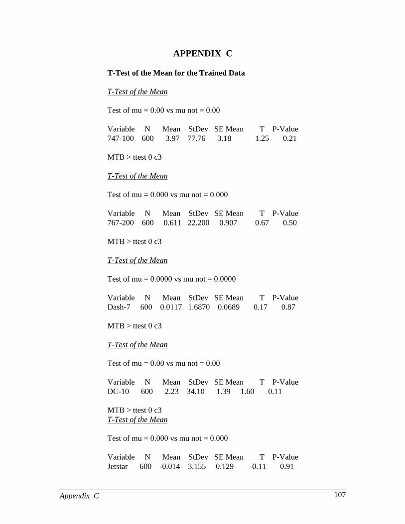
Appendix C 107
APPENDIX C
T-Test of the Mean for the Trained Data
T-Test of the Mean
Test of mu = 0.00 vs mu not = 0.00
Variable N Mean StDev SE Mean T P-Value747-100 600 3.97 77.76 3.18 1.25 0.21
MTB > ttest 0 c3
T-Test of the Mean
Test of mu = 0.000 vs mu not = 0.000
Variable N Mean StDev SE Mean T P-Value767-200 600 0.611 22.200 0.907 0.67 0.50
MTB > ttest 0 c3
T-Test of the Mean
Test of mu = 0.0000 vs mu not = 0.0000
Variable N Mean StDev SE Mean T P-ValueDash-7 600 0.0117 1.6870 0.0689 0.17 0.87
MTB > ttest 0 c3
T-Test of the Mean
Test of mu = 0.00 vs mu not = 0.00
Variable N Mean StDev SE Mean T P-ValueDC-10 600 2.23 34.10 1.39 1.60 0.11
MTB > ttest 0 c3T-Test of the Mean
Test of mu = 0.000 vs mu not = 0.000
Variable N Mean StDev SE Mean T P-ValueJetstar 600 -0.014 3.155 0.129 -0.11 0.91
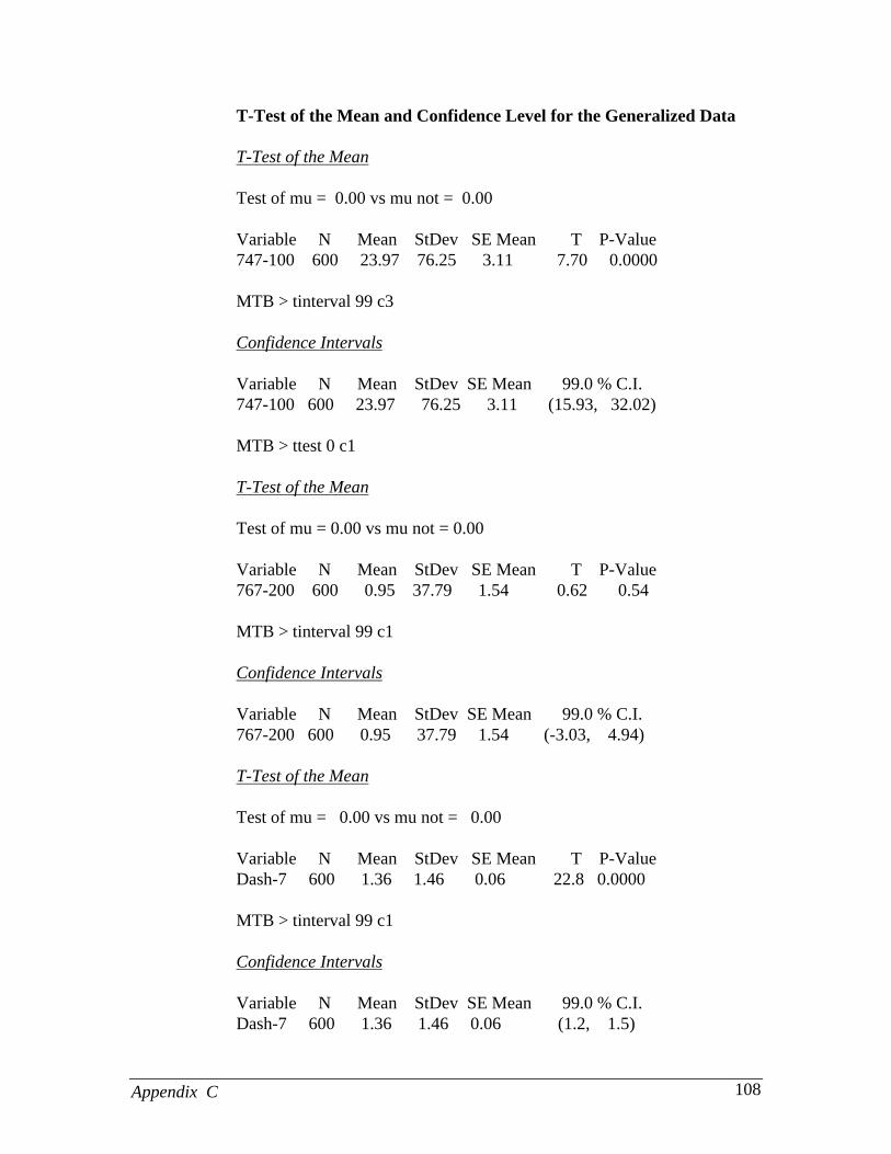
Appendix C 108
T-Test of the Mean and Confidence Level for the Generalized Data
T-Test of the Mean
Test of mu = 0.00 vs mu not = 0.00
Variable N Mean StDev SE Mean T P-Value747-100 600 23.97 76.25 3.11 7.70 0.0000
MTB > tinterval 99 c3
Confidence Intervals
Variable N Mean StDev SE Mean 99.0 % C.I.747-100 600 23.97 76.25 3.11 (15.93, 32.02)
MTB > ttest 0 c1
T-Test of the Mean
Test of mu = 0.00 vs mu not = 0.00
Variable N Mean StDev SE Mean T P-Value767-200 600 0.95 37.79 1.54 0.62 0.54
MTB > tinterval 99 c1
Confidence Intervals
Variable N Mean StDev SE Mean 99.0 % C.I.767-200 600 0.95 37.79 1.54 (-3.03, 4.94)
T-Test of the Mean
Test of mu = 0.00 vs mu not = 0.00
Variable N Mean StDev SE Mean T P-ValueDash-7 600 1.36 1.46 0.06 22.8 0.0000
MTB > tinterval 99 c1
Confidence Intervals
Variable N Mean StDev SE Mean 99.0 % C.I.Dash-7 600 1.36 1.46 0.06 (1.2, 1.5)

Appendix C 109
T-Test of the Mean and Confidence Level for the Generalized Data
T-Test of the Mean
Test of mu = 0.00 vs mu not = 0.00
Variable N Mean StDev SE Mean T P-ValueDC10-30 600 32.80 58.70 2.40 13.71 0.0000
MTB > tinterval 99 c1
Confidence Intervals
Variable N Mean StDev SE Mean 99.0 % C.I.DC10-30 600 32.80 58.70 2.40 (26.7, 39.1)
T-Test of the Mean
Test of mu = 0.00 vs mu not = 0.00
Variable N Mean StDev SE Mean T P-ValueJetstar 600 2.05 5.72 0.23 8.8 0.0000
MTB > tinterval 99 c1
Confidence Intervals
Variable N Mean StDev SE Mean 99.0 % C.I.Jetstar 600 2.05 5.72 0.23 (1.45, 2.65)
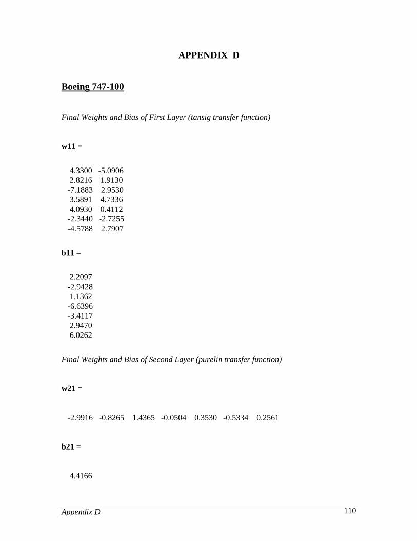
Appendix D 110
APPENDIX D
Boeing 747-100
Final Weights and Bias of First Layer (tansig transfer function)
w11 =
4.3300 -5.0906 2.8216 1.9130 -7.1883 2.9530 3.5891 4.7336 4.0930 0.4112 -2.3440 -2.7255 -4.5788 2.7907
b11 =
2.2097 -2.9428 1.1362 -6.6396 -3.4117 2.9470 6.0262
Final Weights and Bias of Second Layer (purelin transfer function)
w21 =
-2.9916 -0.8265 1.4365 -0.0504 0.3530 -0.5334 0.2561
b21 =
4.4166
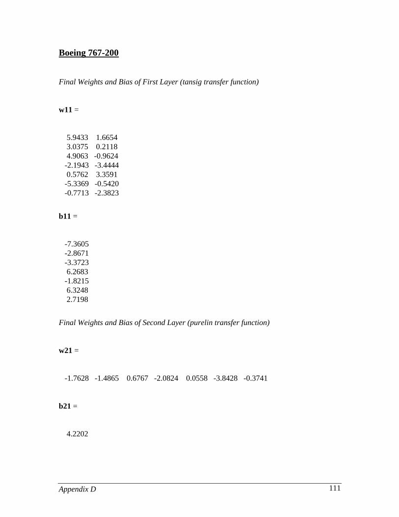
Appendix D 111
Boeing 767-200
Final Weights and Bias of First Layer (tansig transfer function)
w11 =
5.9433 1.6654 3.0375 0.2118 4.9063 -0.9624 -2.1943 -3.4444 0.5762 3.3591 -5.3369 -0.5420 -0.7713 -2.3823
b11 =
-7.3605 -2.8671 -3.3723 6.2683 -1.8215 6.3248 2.7198
Final Weights and Bias of Second Layer (purelin transfer function)
w21 =
-1.7628 -1.4865 0.6767 -2.0824 0.0558 -3.8428 -0.3741
b21 =
4.2202

Appendix D 112
Bombardier Dash-7
Final Weights and Bias of First Layer (tansig transfer function)
w11 =
1.8984 -0.1980 -5.5588 0.9014 3.8653 0.6499 2.4640 0.5639 9.5165 0.3771 -0.7353 1.2700 -0.5016 -0.7420
b11 =
-2.0500 4.0909 -2.7994 -1.8912 -9.6398 -0.2296 0.7715
Final Weights and Bias of Second Layer (purelin transfer function)
w21 =
-18.4723 -1.2817 -6.4901 20.4800 2.0058 2.8261 16.9011
b21 =
-10.4035

Appendix D 113
McDonnel-Douglas DC10-30
Final Weights and Bias of First Layer (tansig transfer function)
w11 =
2.8067 -2.3443 2.3617 0.1115 -4.2343 -2.0659 -7.9688 2.6974 -4.8719 1.4929 0.2293 -0.3729 2.6228 -0.3914
b11 =
-1.8534 -2.1917 7.9116 4.0465 3.5858 -4.2763 -2.2856
Final Weights and Bias of Second Layer (purelin transfer function)
w21 =
-0.6066 6.4040 -10.4683 -0.5452 -5.0632 -3.5148 -15.7285
b21 =
4.5926
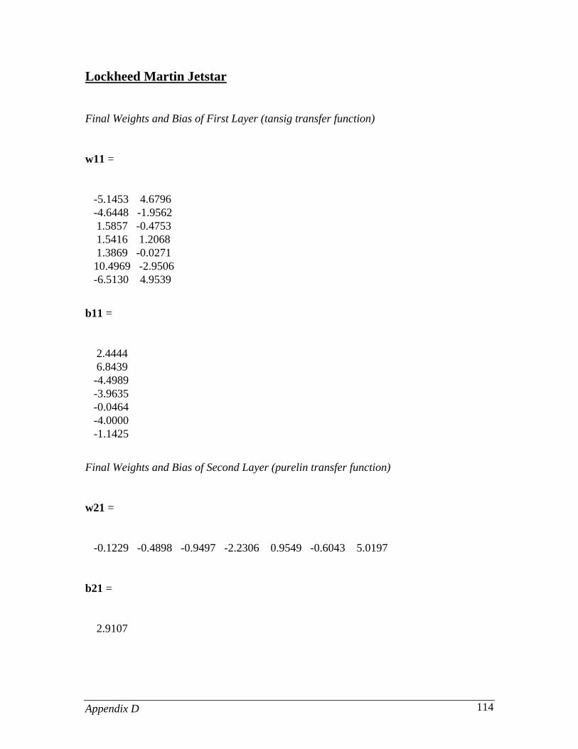
Appendix D 114
Lockheed Martin Jetstar
Final Weights and Bias of First Layer (tansig transfer function)
w11 =
-5.1453 4.6796 -4.6448 -1.9562 1.5857 -0.4753 1.5416 1.2068 1.3869 -0.0271 10.4969 -2.9506 -6.5130 4.9539
b11 =
2.4444 6.8439 -4.4989 -3.9635 -0.0464 -4.0000 -1.1425
Final Weights and Bias of Second Layer (purelin transfer function)
w21 =
-0.1229 -0.4898 -0.9497 -2.2306 0.9549 -0.6043 5.0197
b21 =
2.9107
Vita 115
VITA
Glenn Douglas Schilling was born in Northport, New York, on September 4,
1969. In May 1992 he graduated from Rochester Institute of Technology (RIT), New
York, with a Bachelor of Science in Civil Engineering. While pursuing his bachelor’s
degree at RIT he was involved with the cooperative education plan (co-op), where he
incorporated one year of work experience into his education. After working two years at a
consulting firm in Long Island New York, he came to Virginia Polytechnic Institute and
State University, Virginia, in the spring of 1994 to pursue his graduate studies. In the
spring of 1997 he completed his degree of Master of Science in Civil Engineering,
specializing in Transportation Engineering.
Mr. Schilling plans on starting his career in the transportation engineering arena
upon graduation at Virginia Polytechnic Institute and State University, Virginia.