Modeling agriculture in the Community Land Model. Drewniak1, J. Song2, J. Prell1, V. R. Kotamarthi1,...

Geosci. Model Dev., 6, 495–515, 2013www.geosci-model-dev.net/6/495/2013/doi:10.5194/gmd-6-495-2013© Author(s) 2013. CC Attribution 3.0 License.

EGU Journal Logos (RGB)

Advances in Geosciences

Open A

ccess

Natural Hazards and Earth System

Sciences

Open A

ccess

Annales Geophysicae

Open A

ccess

Nonlinear Processes in Geophysics

Open A

ccess

Atmospheric Chemistry

and Physics

Open A

ccess

Atmospheric Chemistry

and Physics

Open A

ccess

Discussions

Atmospheric Measurement

Techniques

Open A

ccess

Atmospheric Measurement

Techniques

Open A

ccess

Discussions

Biogeosciences

Open A

ccess

Open A

ccess

BiogeosciencesDiscussions

Climate of the Past

Open A

ccess

Open A

ccess

Climate of the Past

Discussions

Earth System Dynamics

Open A

ccess

Open A

ccess

Earth System Dynamics

Discussions

GeoscientificInstrumentation

Methods andData Systems

Open A

ccess

GeoscientificInstrumentation

Methods andData Systems

Open A

ccess

Discussions

GeoscientificModel Development

Open A

ccess

Open A

ccess

GeoscientificModel Development

Discussions

Hydrology and Earth System

Sciences

Open A

ccess

Hydrology and Earth System

Sciences

Open A

ccess

Discussions

Ocean Science

Open A

ccess

Open A

ccess

Ocean ScienceDiscussions

Solid Earth

Open A

ccess

Open A

ccess

Solid EarthDiscussions

The Cryosphere

Open A

ccess

Open A

ccess

The CryosphereDiscussions

Natural Hazards and Earth System

Sciences

Open A

ccess

Discussions

Modeling agriculture in the Community Land Model

B. Drewniak1, J. Song2, J. Prell1, V. R. Kotamarthi 1, and R. Jacob3

1Environmental Science Division, Argonne National Laboratory, 9700 S. Cass Ave, Argonne, IL 60439, USA2Northern Illinois University, Department of Geography, Davis Hall, Room 118, DeKalb, IL 60115, USA3Mathematics and Computer Science Division, Argonne National Laboratory, 9700 S. Cass Ave, Argonne, IL 60439, USA

Correspondence to:B. Drewniak ([email protected])

Received: 29 October 2012 – Published in Geosci. Model Dev. Discuss.: 11 December 2012Revised: 22 March 2013 – Accepted: 26 March 2013 – Published: 19 April 2013

Abstract. The potential impact of climate change on agri-culture is uncertain. In addition, agriculture could influenceabove- and below-ground carbon storage. Development ofmodels that represent agriculture is necessary to addressthese impacts. We have developed an approach to integrateagriculture representations for three crop types – maize, soy-bean, and spring wheat – into the coupled carbon–nitrogenversion of the Community Land Model (CLM), to help ad-dress these questions. Here we present the new model, CLM-Crop, validated against observations from two AmeriFluxsites in the United States, planted with maize and soybean.Seasonal carbon fluxes compared well with field measure-ments for soybean, but not as well for maize. CLM-Cropyields were comparable with observations in countries suchas the United States, Argentina, and China, although thegenerality of the crop model and its lack of technologyand irrigation made direct comparison difficult. CLM-Cropwas compared against the standard CLM3.5, which simu-lates crops as grass. The comparison showed improvementin gross primary productivity in regions where crops arethe dominant vegetation cover. Crop yields and productivitywere negatively correlated with temperature and positivelycorrelated with precipitation, in agreement with other mod-eling studies. In case studies with the new crop model look-ing at impacts of residue management and planting date oncrop yield, we found that increased residue returned to thelitter pool increased crop yield, while reduced residue re-turns resulted in yield decreases. Using climate controls tosignal planting date caused different responses in differentcrops. Maize and soybean had opposite reactions: when lowtemperature threshold resulted in early planting, maize re-sponded with a loss of yield, but soybean yields increased.Our improvements in CLM demonstrate a new capability in

the model – simulating agriculture in a realistic way, com-plete with fertilizer and residue management practices. Re-sults are encouraging, with improved representation of hu-man influences on the land surface and the potentially result-ing climate impacts.

1 Introduction

The role of agriculture in the biosphere has important im-plications for climate change. Humans have influenced 42–68 % of the land surface (Hurtt et al., 2006) through activitiesrelated to cultivation, wood harvesting, and grazing. Glob-ally, around 12 % of the land is currently used for agricul-ture, and in the United States cultivation accounts for roughly20 % of the land base (http://faostat.fao.org). Even thoughthese numbers represent a significant area of land, most Earthsystem models either ignore agriculture or represent cultiva-tion in a simplistic way without management or harvest ac-tivities.

Climate change can have a significant impact on cropyields. Increasing demand for agricultural products from in-creasing worldwide population places changes in crop yieldsat the center of climate change impacts on human soci-eties (Parry et al., 2004; Fischer et al., 2005). Past studieshave shown that increased temperatures and extreme precip-itation events have a negative impact on yield for some crops(Rosenzweig et al., 2002; Lobell and Field, 2007; Osborne etal., 2009; Schlenker and Roberts, 2009; Lobell et al., 2011),offsetting some of the technological advances in crop devel-opment (Lobell and Field, 2007; Lobell et al., 2011). Urbanet al. (2012) predicted that future climate variability couldbe responsible for a decreasing trend of crop yields and an

Published by Copernicus Publications on behalf of the European Geosciences Union.

http://faostat.fao.org

496 B. Drewniak et al.: Modeling agriculture in CLM

increase in yield variability, although some variability mightbe mitigated through adaptation strategies.

Agriculture can also have a significant influence on cli-mate change through biophysical responses to surface fluxesof CO2 and NOx, albedo, and heat fluxes, as well as bio-chemical responses from soil carbon cycling. For exam-ple, irrigation and reduced tillage on croplands resulted ina global cooling effect, while local effects for precipitation,cloud cover, and radiation were stronger (Lobell et al., 2006;Diffenbaugh, 2009).

Cultivation also impacts the carbon stored and releasedfrom soil. Loss of soil carbon as a result of native vegetationremoval can be significant, with long payback times (Far-gione et al., 2008; Gibbs et al., 2008; Searchinger et al.,2008). The influence of crops on carbon cycling varies withmanagement practices such as crop rotation, tillage, fertilizerinputs, and residue harvesting (West and Post, 2002; Hookeret al., 2005; Dou and Hons, 2006; Huggins et al., 2007; Khanet al., 2007; Kim et al., 2009). Although observations dis-agree on the magnitude and in some cases the sign of carbonchange, most do agree that management influences the totalsoil carbon stored.

The strong atmosphere–land surface coupling and the pro-nounced influence of agriculture on the biosphere makethe inclusion of crops important and necessary for evaluat-ing atmosphere–biosphere interactions. As the need for im-proved land surface models and the importance of distur-bance on biogeochemical cycles were recognized, new mod-els that include agriculture began to emerge. Several stud-ies have incorporated agriculture into a vegetation modelingframework to improve estimates of carbon and nitrogen cy-cling in the soil system (Kucharik and Brye, 2003; Bondeauet al., 2007; Osborne et al., 2007; Smith et al., 2010; Leviset al., 2012). Agro-IBIS (Agro-Integrated Biosphere Simula-tor; Kucharik and Brye, 2003), which was designed to sim-ulate maize, soybean, and wheat crop types across the con-tinental United States, has been tested against flux measure-ments (Kucharik and Twine, 2007). Agro-IBIS was used toevaluate yield variability against nitrogen inputs (Kucharikand Brye, 2003) and planting date (Kucharik, 2008) and hasundergone yield sensitivity analysis (Kucharik, 2003). TheLPJ-mL (Lund–Potsdam–Jenna-managed land; Bondeau etal., 2007) agriculture model combines a dynamic vegetationmodel with several crop types, represented much like natu-ral vegetation through the use of crop functional types. Thisallows the model to capture growth on a global scale. LPJ-mL was used to evaluate future water and carbon fluxes asa result of land use change, management, and CO2 fertil-ization. Although LPJ-mL does include a fertilizer repre-sentation through influences on leaf area index (LAI), themodel does not include nutrient cycling, which might im-pact plant development as a result of nitrogen stress. Os-borne et al. (2007) developed a coupled crop–climate modelto evaluate the influence of crops on climate by incorporat-ing the General Large Area Model (GLAM), a groundnut

model that can be applied to other tropical crop types, intothe Hadley Center Atmospheric Model (HadAM3). The fo-cus of the study was in the tropics, using temperature and soilmoisture to interactively determine crop management such ascultivation area, sowing date, and growing season. Osborneet al. (2009) noted the correlation between climate and cropyield variability and additionally found that crop yield vari-ability had an impact on temperature, though not necessarilyon precipitation. The ORCHIDEE-STICS (Organizing Car-bon and Hydrology in Dynamic Ecosystems–Supra-ThermalIon Composition Spectrometer; Smith et al., 2010) modelfocuses on the European crops soybean, maize, and winterwheat and uses an automated fertilizer and irrigation schemewhen plants become stressed, but it does not include explicitcrop organ development and residue management.

Recently, a more sophisticated crop model was incorpo-rated into the Community Land Model (Levis et al., 2012).This addition adds a separate growth scheme for crops tosimulate maize, soybean, and cereals in the midlatitudes,using algorithms from the Agro-IBIS model (Kucharik andBrye, 2003). Levis et al. (2012) used the new developmentto evaluate CO2 fluxes from the modified LAI. The modelshowed promising improvements in annual net ecosystemexchange and the impact agriculture has on climate, such asreduced precipitation. However, this model lacked some im-portant features of nitrogen cycling (nitrogen retranslocation,soybean nitrogen fixation) and management practices (fertil-izer, residue harvest) that may have an important impact onthe carbon fluxes.

We chose the coupled carbon–nitrogen version of theCommunity Land Model (CLM [CLM-CN]; Thornton andZimmerman, 2007; Oleson et al., 2008; Stockli et al., 2008)as a basis for our model, because CLM-CN already hada comprehensive carbon–nitrogen scheme, allowed multipleplant functional types (PFTs) to exist within a grid cell, andintegrated crops as a model component (although they wererepresented as grass). In addition, CLM-CN was already cou-pled to the atmosphere and ocean in the Community ClimateSystem Model version 3 (CCSM3.0) and beyond, providingan opportunity for future studies on feedbacks between cli-mate change and agricultural productivity. We expanded thePFTs in CLM-CN to include specific crop types, allowingthem to share space but exist separately, so as not to com-pete for resources with natural vegetation. Our new model,CLM-Crop, presented in this paper, includes new physiologyand carbon schemes to describe maize, soybean, and springwheat. We investigate the ability of CLM-Crop to simulateagriculture environments through calculated harvest yields,LAI, and gross primary productivity (GPP). In addition, weinclude a capability for varying residue management and fer-tilizer. We do not consider tillage practices, because CLM-Crop’s carbon pools are not distributed in the soil profile.We note that although CLM-Crop is designed to be imple-mented globally, a majority of the parameterizations are typ-ical of crops grown in the United States; therefore we focus

Geosci. Model Dev., 6, 495–515, 2013 www.geosci-model-dev.net/6/495/2013/

B. Drewniak et al.: Modeling agriculture in CLM 497

our analysis on this region, with some limited discussion onthe global results.

Several features of CLM-Crop will be included in the nextrelease of CLM; we will point out those features throughoutthe model development section. The description of CLM-Crop in Sect. 2 includes a breakdown of the simulationsperformed. Section 3 evaluates the model’s performancethrough comparison with observations and a standard grasssimulation. Next, case studies demonstrate the impact ofresidue management and planting date on yield and GPP inSect. 4. A discussion follows in Sect. 5.

2 Methods

2.1 Description of the Crop Module (CLM-Crop)

The standard CLM3.5, which simulates land surface re-sponse to climate forcing, has been tested extensively againstobservations, both as a component of the CCSM3.0 and of-fline (Oleson et al., 2008; Stockli et al., 2008). The CLM op-tional feature to include carbon and nitrogen cycling (CLM-CN) was discussed by Thornton and Zimmerman (2007).However, crops in CLM-CN are generic, modeled as grasseswithout biomass removal during harvest and without variedcarbon allocation during different growth stages. Therefore,we have added three additional PFTs to the model to repre-sent maize, soybean, and spring wheat crop types. We beganour evaluation with these three types, because (1) maize oc-cupies that largest share of cultivated land in North Amer-ica, with the expectation of an even larger share in the fu-ture as a major ethanol fuel source; (2) soybean is the sec-ond largest crop cultivated in North America, grows rapidlyin South America, and is a potential biodiesel crop; and(3) spring wheat is the primary cereal crop produced all overthe world. All three crops have been studied extensively andhave known phenology.

CLM-Crop has a sub-grid hierarchy allowing multiplePFTs to exist in a single soil column and multiple soilcolumns to exist in a grid cell (Fig. 1). Each soil column hasits own carbon and nitrogen pools, so vegetation growing inone column does not compete for resources with vegetationin a separate column. We separate crops from natural vege-tation to model them independently. For example, a grid cellgrowing maize and soybean in addition to natural trees andgrasses will have at least three soil columns: one contain-ing natural vegetation PFTs, one containing maize, and onecontaining soybean. Although they share the space on a gridcell, each soil column has separate dynamics for soil water,litter, soil organic carbon, etc., consistent with the vegetationin that column.

2.1.1 Growth scheme

The growth and development processes of crops are bro-ken into four stages (similar to Levis et al., 2012): seeding,

Fig. 1. An example of the sub-grid hierarchy in CLM-Crop (basedon concepts of Oleson et al., 2004).

emergence, organ development, and harvest. Each phase ischaracterized by varied carbon allocation between the com-ponents of the plant: leaves, stems, roots, and grain. Thegrowth stage is determined by the fraction of phenologicalheat units (FPHUs) accumulated (Table 1), relative to thecrop planting date. The FPHUs for each growth stage aresimilar to those in the Agro-IBIS model (Kucharik and Brye,2003). FPHUs are calculated as

FPHU=

current day∑i=planting

HUi

PHU, (1)

where PHU is the total number of phenological heatunits (PHUs) necessary to reach maturity. At planting, heatunits (HUs) are accumulated daily as

HU = Tave− Tbase, (2)

where Tave is the average 2 m air temperature for thecurrent day, andTbase is the minimum temperature re-quired for growth, as in the SWAT (Soil Water AssessmentTool) model (Neitsch et al., 2005). The total number ofPHUs necessary to reach maturity, derived by the Sacks etal. (2010) Crop Calendar Dataset, varies spatially and withcrop species (described in Sect. 2.2). PHUs were originallycalculated from a base temperature of 5◦C, so we use 5◦Cas a base temperature for all crops. Because growth stagesfor plant development are determined by the fraction of totalPHUs, this approach is reasonable, even though actual base

www.geosci-model-dev.net/6/495/2013/ Geosci. Model Dev., 6, 495–515, 2013


temperature is 0◦C for spring wheat and ranges from 8 to10◦C for maize and soybean. For grid cells where PHU dataare not included in the Crop Calendar Dataset, a default PHUvalue is used (Table 1).

The planting date is fixed for each crop and is based on theaverage planting date from Sacks et al. (2010). At planting,small amounts of carbon (approximately equivalent to thecarbon content in seeds) and nitrogen (Table 1) are allocatedto the leaves to initiate photosynthesis for growth, but furthercarbon allocation is withheld until the crop has reached theemergence phase. The fraction of available carbon allocatedhourly to each plant component (leaves, roots, and stems)during the remaining growth period follows the Agro-IBISmodel (Kucharik and Brye, 2003), as was also done by Leviset al. (2012). Between emergence and organ development,carbon is directed toward leaves, roots, and stems. Root de-velopment assimilates 30–50 % of carbon initially; this valuedecreases with PHU accumulation to 5 % by maturity (Ta-ble 1), while the remaining carbon is allocated to leaves andstems.

Once organ development begins, carbon directed to leavesand stems decreases rapidly, and the majority of carbon isappropriated to grain, while a small amount is filtered tothe roots (Table 1). Throughout the growth period, photo-synthesis is limited by the availability of water and nitrogenthrough a downregulation process. The grain fill features ofthis model differ from the Levis et al. (2012) crop modelthrough the maintenance of a separate pool for organ car-bon and nitrogen to keep track of yield, whereas Levis etal. (2012) allocate grain carbon into the stem pool.

2.1.2 Nitrogen and retranslocation

Nitrogen allocation for crops follows that of natural vege-tation, which is based on carbon:nitrogen (CN) ratios forleaves, stems, roots, organs, and litter. Nitrogen demand dur-ing organ development is fulfilled through retranslocationfrom leaves, stems, and roots (Pollmer et al., 1979; Crawfordet al., 1982; Simpson et al., 1983; Ta and Weiland, 1992; Bar-bottin et al., 2005; Gallais et al., 2006, 2007). Because mostCN ratio measurements are from mature crops, we estab-lished pre- and post-grain-development CN ratios for leaves,stems, and roots (Table 1). Prior to organ development, CNratios are optimized to allow maximum nitrogen accumula-tion for later use during organ development. When grain fillbegins, nitrogen from the leaves, stems, and roots (for wheat)is transferred to a retranslocation pool, such that the new CNratio for each plant part is the same as for crop residue. Theorgan nitrogen demand is first supplied from the retranslo-cated nitrogen pool, and any remaining demand is drawnfrom the soil nitrogen pools. The retranslocation scheme isincluded in the next release of CLM4.5.

2.1.3 Fertilization

In CLM, the denitrification rate is high, resulting in a 50 %loss of the unused available nitrogen each day. To integratefertilizer into the model without significant loss of fertilizerduring the early stages of growth when nitrogen demand islow and availability is high, we adopted a fertilizer schemedelivering nitrogen directly to the soil mineral nitrogen poolover a 20 day period, beginning at emergence. The schemecan effectively reduce large losses of nitrogen due to leach-ing and denitrification during the early stage of crop devel-opment. The 20 day period was chosen as an optimizationtool to limit fertilizer application to the emergence stage.Total nitrogen fertilizer amounts are 150 kg ha−1 for maize,80 kg ha−1 for wheat, and 25 kg ha−1 for soybean, repre-sentative of current annual fertilizer application rates in theUnited States (http://www.ers.usda.gov/Data/FertilizerUse).The fertilizer scheme is included for the release of CLM4.5.

2.1.4 Soybean nitrogen fixation

Nitrogen fixation by soybean is similar to that in the SWATmodel (Neitsch et al., 2005) and is dependent on soil mois-ture, nitrogen availability, and growth stage. If soil nitrogenis sufficient to meet soybean demand, no fixation will occurduring the time step. Nitrogen fixation is largest during theearly to middle growth stages, when demand for nitrogen isgreatest. Soybean fixation is dependent on soil water, nitro-gen availability, and the growth stage of the crop, determinedby

Nfix = Nplant ndemand∗ min(1,f xw,f xn) ∗ f xg, (3)

where Nplant ndemand is the balance of nitrogen needed toreach potential growth that cannot be supplied from the soilmineral nitrogen pool,fxw is the soil water factor,fxn is thesoil nitrogen factor, andfxg is the growth stage factor calcu-lated by

f xw =wf

0.85, (4)

f xn =

0 forsminn ≤ 101.5− 0.005∗ (sminn ∗ 10) for10< sminn ≥ 30

1 forsminn > 30, (5)

f xg =

0 for PHU≤ 0.15

6.67∗ PHU−1 for0.15< PHU≥ 0.301 for 0.30< PHU≥ 0.55

3.75− 5∗ PHU for0.55< PHU≥ 0.750 for PHU≥ 0.75

, (6)

wherewf is the soil water content as a fraction of the water-holding capacity for the top 0.5 m,sminnis the total nitrogenin the soil pool (g m−2), and PHU is the fraction of growingdegree days accumulated during the growth period.Nfix is


http://www.ers.usda.gov/Data/FertilizerUse


Table 1.Crop parameters.

Parameter Maize Wheat Soybean

FPHUs for growth stagesSeeding 0 0 0Emergence 0.03 0.08 0.03Grain fill 0.53 0.59 0.70Harvest 1 1 1

Pre-grain-fill-stage CN ratio

Leaf 10 15 25Stem 50 50 50Root 42 30 42Organ 50 40 60

Post-grain-fill-stage CN ratio

Leaf 65 65 65Stem 120 100 130Root 42 40 42Organ 50 40 60

Other parameters

Base temperature 5◦C 5◦C 5◦CInitial carbon allocation to seed (g C m−2) 0.8 3.9 2.5Initial root carbon allocation 40 % 30 % 50 %Initial leaf carbon allocation Depends on FPHUInitial stem carbon allocation Depends on FPHUFinal root carbon allocation 5 % 5 % 5 %Final leaf carbon allocation 0 % 0 % 0 %Final stem carbon allocation 5 % 5 % 5 %Maximum LAI 5.0 7.0 6.0Maximum harvest index 0.6 0.5 0.38Default PHU 1600 1900 1000Maximum root depth (m) 1.2 0.9 1.6

added directly to the soil mineral nitrogen pool for use inthat time step. Nitrogen fixation does not occur in the earlygrowth stage, before the plant accumulates 15 % of PHU, orin the late growth stage, after 75 % of PHUs have accrued(shortly after grain fill begins). The soybean fixation schemewill also be added to the CLM4.5 crop model.

2.1.5 Crop root structure

In CLM-CN, vegetation has a constant root depth and densityprofile; root density decreased linearly with depth. In Levis etal. (2012), root density for all vegetation decreased exponen-tially with depth, but for crops it did not vary with growth.We incorporated into CLM-Crop a dynamic root scheme toapproximate fine root distribution and rooting depth in re-sponse to environmental conditions.

The root depth for natural vegetation is held constant andis dependent on the type of PFT (Oleson et al., 2004). Cropshave a dynamic rooting depth that depends on growth stage.Crop root depth, which is 4 cm at planting, continues to grow

linearly with FPHU until a maximum depth is reached at thebeginning of the organ development stage. The gradual in-crease in root depth is meant to simulate a young crop with-standing dry soil profiles. Maximum root depths for maize,wheat, and soybean are 120 cm, 90 cm, and 160 cm, respec-tively (Mayaki et al., 1976; Araki and Iijima, 2001; Amosand Walters, 2006).

The fine root carbon budget in each soil layer depends onnew carbon allocation and turnover loss at each time step.Fine root carbon,Ci (kg m−2), in each soil layer (i) is calcu-lated as

Ci = Ci,0 + rd,iCnew− RiCloss, (7)

where

rd,i = (1− f )rw,i + f rn,i . (8)

The new carbon (Cnew) allocation is based on a redistribu-tion factor (rd,i) for each soil layer that links soil moistureand nutrient uptake capacity by weighting the relative avail-able soil moisture (rw,i) and the relative nutrient distribution



(rn,i) by the root zone water availability factor (f ), wheref

ranges from 0 for soil at the wilting point to 1 for saturatedsoil. The distribution algorithm for new fine roots combinesthe availability of two essential substances – water and nu-trients – for root uptake and allows for root plasticity withnon-uniform water distribution (Mayaki et al., 1976; Garayand Wilhelm, 1983; Amos and Walter, 2006). Carbon loss(Closs) due to root turnover is removed from each layer rela-tive to the fine root fraction (Ri) in the soil layer.

The prescribed relative nutrient profile used to calculatern,i is the approximated nitrogen profile based on Jobbagyand Jackson (2001) and the global soil profile data set of Bat-jes (2008). This profile has constant nitrogen in the top soillayers (less than 10 cm depth), decreasing linearly to zero atthe bottom of the last soil layer. This distribution is charac-teristic of agricultural soils where past tillage practices havehomogenized the upper soil profiles (Blanco-Canqui and Lal,2008).

2.1.6 Harvest management

Crops are harvested as soon as maturity is reached, as wasdone by Levis et al. (2012). However, in CLM-Crop, harvestis partitioned between the atmosphere and litter pools. All ofthe carbon and nitrogen in the grain, along with a percentageof carbon and nitrogen in the leaves and stems, is harvestedand respired to the atmosphere. The remaining above-groundand all of the below-ground carbon and nitrogen are consid-ered residue and are returned to the litter pool as such, sim-ulating residue management practices. Variability of residueamounts in CLM-Crop enables study of the impact of differ-ent residue management practices on soil carbon.

2.2 Input data

2.2.1 Climate

Simulations required three-hourly data for temperature, windspeed, humidity, precipitation, solar radiation, and surfacepressure from the National Center for Environmental Pre-diction (NCEP) reanalysis data for the period 1948–2004,as described by Kalnay et al. (1996). We cycled through theNCEP reanalysis data to spin up the model and reach a steadystate of carbon and nitrogen in the soil (Thornton and Rosen-bloom, 2005). CLM-Crop was run at a resolution of 2.8◦ lat-itude by 2.8◦ longitude.

2.2.2 Land use

Natural vegetation cover in CLM-Crop was represented by14 PFTs, whose abundance was based on satellite data de-scribed by Bonan et al. (2002). Natural vegetation PFTs in-cluded needleleaf evergreen and deciduous trees, broadleafevergreen and deciduous trees, shrubs, and grasses, all ofwhich were divided among boreal, temperate, and tropicalregions. We used data from Leff et al. (2004) to derive crop

coverage maps representative of the year 1992, by separatingindividual crop types of maize, soybean, and wheat from thetotal crop area of Bonan et al. (2002). Remaining crop areanot designated as maize, soybean, or wheat was attributed toan alternative PFT, called “other crop,” which was modeledas a C3 grass. Because crop area data sets did not distinguishwinter wheat from spring wheat, we included winter wheatareas in our spring wheat data. Double cropping was also in-cluded in the data sets, causing total crop area to be countedtwice in some grid cells of CLM-Crop.

2.2.3 Planting date and PHUs

The planting date for each crop was derived from the CropCalendar Dataset (Sacks et al., 2010). Spatial planting datafor maize, soybean, and spring wheat were based on the av-erage planting date, aggregated from 5 min resolution to 2.8◦

for use in CLM-Crop. PHUs were also based on Sacks etal. (2010), calculated from the average number of HUs be-tween the average planting and harvest dates, which weredetermined by regional climatology from the CRU data set(New et al., 1999) for the years 1961–1990. The Crop Calen-dar Dataset accounts for generalized planting dates over largeregions from the dominant crop cover, using nearest neighborextrapolation over regions where data is not available. Thedata set does not capture small-scale variability in plantingboth spatially and temporally (Sacks et al., 2010); however,as our resolution is course, we believe that this database isappropriate for this application. We did not consider doublecropping or crop rotation in CLM-Crop.

2.3 Model simulation

An accelerated spin-up procedure (Thornton and Rosen-bloom, 2005) was used to build up soil organic carbon lev-els in CLM-Crop, with natural vegetation only (crop ar-eas simulated as C3 grass). Once soil carbon and nitro-gen pools reached steady state, the land use was convertedto include croplands. Our agriculture scenario (hereafterCROP) was established to simulate current managementand fertilizer practices and represent the agricultural prac-tices common over the United States during the last decade(www.usda.gov). We compared these results with a grass-land scenario (hereafter GRASS) that included the land coverused in the spin-up (i.e., with crops simulated as C3 grass).Each scenario was run for three complete cycles of the 1948–2004 climate data (a total of 171 yr) at an hourly time step toreach a steady state. The last 57 yr of each simulation (onecycle of 1948–2004) was included in results that show av-eraged data. We focused our evaluation on comparisons ofCROP with observations and GRASS. In addition, we con-sidered four case studies to evaluate the impact of residuereturns and a climate-induced planting date on crop yield andGPP.



3 Results

3.1 Model performance compared with observations

3.1.1 CO2 fluxes

For crops, CO2 flux data are available from two sites inthe AmeriFlux network (http://public.ornl.gov/ameriflux):Bondville, IL (40.01◦ N, 88.29◦ W) and a rain-fed site inMead, NE (41.18◦ N, 96.43◦ W). These sites are chosen be-cause they contain GPP (the rate of carbon captured andstored for growth in the plant through photosynthesis), netecosystem exchange (NEE; GPP minus the total ecosystemautotrophic and heterotrophic respiration), and LAI data fora maize–soybean rotation. Although GPP is not directly mea-sured at AmeriFlux stations, GPP is calculated in the Amer-iFlux Level 4 data as the difference between ecosystem res-piration and NEE. Ecosystem respiration is estimated usingReichstein et al. (2005), and NEE data are gap-filled by us-ing the artificial neural network method (Papale and Valen-tini, 2003). In the absence of observations with spring wheat,we discuss only maize and soybean. Both sites were plantedwith maize in 2001 and with soybean in 2002. For compar-ison purposes, since CLM-Crop is run at a global resolutionof 2.8◦, we chose the grid cell closest to the site. In this case,the grid cell central coordinates are 40.46◦ N, 87.19◦ W forBondville and 40.46◦ N, 95.625◦ W for Mead.

Peak monthly average GPP for maize is observed duringthe middle of the growth period, when LAI peaks. CROPsimulates lower GPP than observations for maize duringthis time for the two sites; however, GPP estimates later inthe growth season are comparable with measured values atBondville and Mead (Fig. 2a, d). The annual total GPP sim-ulated by CLM-Crop is 1197 g C m−2 yr−1, which is compa-rable to observations of 1168 g C m−2 yr−1 at Bondville. Atthe Mead site, the simulated GPP total of 1199 g C m−2 yr−1

is lower than observed values of 1370 g C m−2 yr−1. CROP-simulated maize GPP drops shortly after fertilizer applica-tion is complete, resuming again during the grain fill stage ofthe growth period, when nitrogen is remobilized. The dropin GPP is the result of nitrogen stress at the end of the fer-tilization period and loss of excess nitrogen due to a highdenitrification factor. Denitrification in CLM-CN accountsfor a 50 % loss of unused nitrogen in the soil. The deni-trification factor was intended to account for losses of ni-trogen in a saturated-nitrogen environment, such as one in-duced by fertilizer inputs. However, since fertilizer is ap-plied over a 20 day period, rapid loss of most of the fertil-izer after the early growth phase causes a nitrogen limitationin maize during the middle growth stages. Because maizehas a higher nitrogen demand than soybean and wheat, lossof unused fertilizer from denitrification results in significantnitrogen limitation for growth. During the late growth pe-riod, remobilization of nitrogen from leaves and stems al-lows grain access, so GPP increases (and peaks) during the

organ development stage. That this is an artifact introducedby rapid denitrification in the current version of CLM iswidely recognized. The nitrogen scheme in the model is un-dergoing a thorough evaluation and reformulation (Tang etal., 2013). The new nitrogen scheme is expected to circum-vent the problem with the current formulation, making thenitrogen availability to maize more uniform and the GPPcalculations closer to observations during the early phaseof the crop growth cycle. NEE (Fig. 2b, e) shows char-acteristics similar to GPP. Although the timing is not al-ways synchronized with observations as a result of our useof fixed values for planting and growth periods, the modeldoes capture the general trend of NEE during the growthperiod for both the Bondville and Mead AmeriFlux sites,demonstrating the model’s ability to simulate ecosystem res-piration. The total annual NEE is underestimated by CLM-Crop; at Bondville, simulated NEE was−322 g C m−2 yr−1

compared to−405 g C m−2 yr−1 observed. At Mead, totalNEE in CLM-Crop was−314 g C m−2 yr−1, but measuredat−545 g C m−2 yr−1.

CROP-simulated GPP for soybean agrees well with ob-servations at Mead, but it increases early and is too high atBondville (Fig. 2g, j). The earlier planting date in the modelcauses GPP at the Bondville site to be offset by more thanone month from observations, while the longer growth pe-riod at Bondville causes modeled GPP to be higher than themeasured value. The annual total simulated GPP at Bondvillefor soybean is 1055 g C m−2 yr−1 versus observations of773 g C m−2 yr−1. Growth period length is well estimated atthe Mead site, and GPP values match observations, althoughtotal annual GPP is overestimated at 904 g C m−2 yr−1 whereobservations indicate 798 g C m−2 yr−1. For soybean, simu-lated GPP is higher than the measured value as a result ofcropping sequence. The lower soybean biomass at the end ofthe growth period decreases the amount of decomposition,and thus nitrogen immobilization, the year following soy-bean planting. However, in a maize–soybean rotation, maizeresidue from the previous year’s crop immobilizes more soilnitrogen for decomposition, leaving less available for soy-bean growth. With no rotation in CLM-Crop and no simu-lation of this phenomenon in the model, more nitrogen be-comes available for growth. Simulated NEE values for soy-bean (Fig. 2h, k) are similar to the corresponding GPP val-ues, however, simulated NEE of−228 g C m−2 yr−1 is over-estimated compared to observations of−25 g C m−2 yr−1.CROP NEE is slightly greater than observations at theBondville site during the growth season because of higherGPP, with annual total values of−257 g C m−2 yr−1 versusobservations of−142 g C m−2 yr−1. To introduce crop rota-tion into the model requires a data set on crop rotation atthe grid scale and a model capability to simulate changesin land use, which currently are not available. As these im-provements become available, we expect to introduce croprotation into the next model update.


http://public.ornl.gov/ameriflux


Fig. 2.Simulated (lines) and observed (circles) monthly averaged gross primary productivity (GPP; g C m−2 day−1), net ecosystem exchange(NEE; g C m−2 day−1), and LAI (m2 m−2) during 2001 and 2002 for maize and soybean at two sites: Bondville, IL (40.01◦ N, 88.29◦ W),and Mead, NE (41.18◦ N, 96.43◦ W).

Global average GPP from 2000 through 2004, simulatedby CROP, shows improvement versus GRASS in compari-son with MODIS satellite data (Zhao et al., 2005), as shownin Fig. 3. In regions with high crop density, GPP is lower inCROP than in GRASS, particularly in the US Midwest, west-ern Brazil, Europe, the United Kingdom, and Asia. Over-all, crop representation improved the root-mean-squared er-ror (RMSE) by a small amount, 3 %; locally, however, in re-gions where croplands are dominant, RMSE shows more sig-nificant improvement (Table 2). For example, in the UnitedStates, France, and Mexico, the RMSE was about 15 % lower

for CROP than for GRASS. In South Africa, Greece, theNetherlands, and Turkey, the RMSE for CROP was morethan 10 % lower, while in the United Kingdom, the RMSEfor CROP was 8 % lower.

3.1.2 Leaf area index

Simulated peak LAI for maize and soybean (Fig. 2c, f, i, l) isgenerally consistent with observations at both the Mead andBondville sites. However, because LAI decline is not simu-lated in the model, LAI values are higher than observationslate in the growth period. This also allows the GPP to remain



Fig. 3. Average GPP (g C m−2 yr−1) for the years 2000–2004,derived from(a) MODIS data (Zhao et al., 2005),(b) CROP, and(c) GRASS.

high in the late growth stages, producing higher yields thanobserved, because more carbon is assimilated in the simula-tion.

The LAI in the model is based on the amount of carbonin the leaves and a constant specific leaf area (SLA; the ratioof leaf area to dry leaf weight) for each crop type; however,observations show that SLA actually varies throughout thegrowth season (Tardieu et al., 1999) and with nitrogen fer-tilizer application methods (Amanullah et al., 2007), causingdiscrepancies between observed and model-simulated LAI.To allow varying SLA with growth period would be diffi-cult, because this requires detailed knowledge of how SLAresponds to climate for each crop during each growth phase.For maize, LAI is overestimated, particularly in the earlygrowing season, despite having less leaf carbon through-out the growth period (Fig. 4a). Soybean LAI values for

Table 2.Root-mean-squared error of GPP for selected regions fromCROP and GRASS simulations, as compared with MODIS satellitedata of Zhao et al. (2005).

Country CROP GRASS Percent Change

United States 510.86 581.77 −12.19France 625.62 751.16 −16.71Mexico 712.22 855.15 −16.71Spain 475.86 505.03 −5.78Italy 809.42 861.61 −6.05Germany 359.30 381.11 −5.72South Africa 240.14 266.87 −10.01Greece 727.64 806.89 −9.82Netherlands 422.54 478.28 −11.65Portugal 801.06 845.56 −5.20Turkey 618.34 684.91 −9.71United Kingdom 431.07 468.62 −8.01

the Mead site are comparable with observations. For theBondville site, soybean LAI values are underestimated de-spite the high GPP; however, the similarity of simulated leafcarbon to observations for this site (Fig. 4d) demonstrates theimportance of variable SLA.

3.1.3 Plant carbon

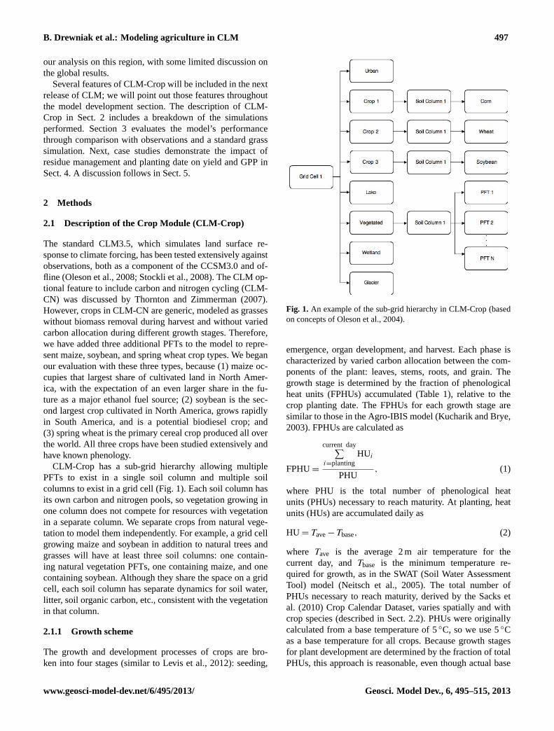
The total carbon distributed in the leaves, stems, and organsof maize and soybean for the Bondville site is shown inFig. 4. Leaf carbon in maize is underestimated by the model,because nitrogen stress constrains growth in the early to mid-dle growth phase, in contrast to field observations. Carbon inthe stem is comparable with observations during the emer-gence stage; however, organ carbon is underestimated by afactor of two. Because organ development relies heavily onretranslocated nitrogen from leaves and stems and becausemaize was limited by nitrogen stress earlier in the growthseason, the lower organ carbon than observations is not sur-prising.

Leaf carbon for soybean is overestimated during most ofthe growth period because of early planting; however, peakleaf carbon agrees with observations. High simulated GPPfor soybean caused stem and organ carbon to be overesti-mated by the model, as compared with field measurements.

Carbon levels for the Mead site were not separated intocrop components, but total carbon in the above-groundbiomass was reported. Our simulated carbon values for maizeand soybean at that rain-fed site are shown in Fig. 5. Peakestimates of above-ground carbon for maize in the modelare similar to observations but are offset because of nitro-gen limitation in the early to middle growth stages. Whennitrogen is remobilized for grain development, total carbonin the plant increases until late in the growth season, be-cause the lack of LAI decline causes the peak carbon tooccur later in the model than in field measurements. Total



Fig. 4. Simulated (lines) and observed (circles) leaf, stem, and organ carbon (g C m−2) during 2001 and 2002 for maize and soybean atBondville, IL.

soybean above-ground carbon is overestimated by the model.Although carbon is modeled well in the early growth season,total plant carbon peaks at higher values versus observationsin the grain fill stage. The early curve and timing of the car-bon growth are simulated well for soybean, and the peak car-bon is simulated well for maize in CROP.

3.1.4 Yields

The average yields estimated by CROP for the last 57 yr ofthe simulation are shown in Fig. 6 for maize, wheat, andsoybean. Direct comparison of yields with observations isdifficult, because CROP does not include improved technol-ogy and management practices (such as irrigation) that affectyield; therefore, our results might differ significantly fromobservations in certain regions and do not include the largeadvances in yield seen over the last several decades. The re-sults presented here should be considered a baseline for cal-culating crop yields in the absence of these additional in-terventions. These results provide a template for assessingthe impacts of management changes in the future as climatemodels become more capable of handling socioeconomicand external interventions in land management and land use.

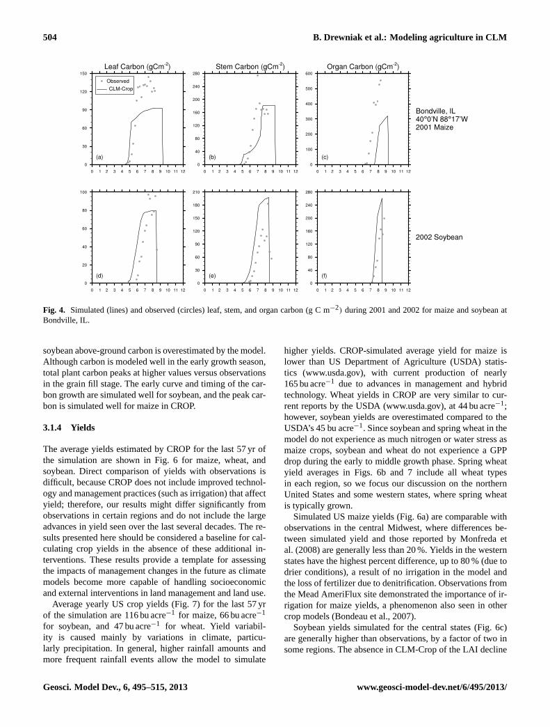
Average yearly US crop yields (Fig. 7) for the last 57 yrof the simulation are 116 bu acre−1 for maize, 66 bu acre−1

for soybean, and 47 bu acre−1 for wheat. Yield variabil-ity is caused mainly by variations in climate, particu-larly precipitation. In general, higher rainfall amounts andmore frequent rainfall events allow the model to simulate

higher yields. CROP-simulated average yield for maize islower than US Department of Agriculture (USDA) statis-tics (www.usda.gov), with current production of nearly165 bu acre−1 due to advances in management and hybridtechnology. Wheat yields in CROP are very similar to cur-rent reports by the USDA (www.usda.gov), at 44 bu acre−1;however, soybean yields are overestimated compared to theUSDA’s 45 bu acre−1. Since soybean and spring wheat in themodel do not experience as much nitrogen or water stress asmaize crops, soybean and wheat do not experience a GPPdrop during the early to middle growth phase. Spring wheatyield averages in Figs. 6b and 7 include all wheat typesin each region, so we focus our discussion on the northernUnited States and some western states, where spring wheatis typically grown.

Simulated US maize yields (Fig. 6a) are comparable withobservations in the central Midwest, where differences be-tween simulated yield and those reported by Monfreda etal. (2008) are generally less than 20 %. Yields in the westernstates have the highest percent difference, up to 80 % (due todrier conditions), a result of no irrigation in the model andthe loss of fertilizer due to denitrification. Observations fromthe Mead AmeriFlux site demonstrated the importance of ir-rigation for maize yields, a phenomenon also seen in othercrop models (Bondeau et al., 2007).

Soybean yields simulated for the central states (Fig. 6c)are generally higher than observations, by a factor of two insome regions. The absence in CLM-Crop of the LAI decline



Fig. 5.Simulated (lines) and observed (circles) total plant carbon (gC m−2) during 2001 and 2002 for maize and soybean at Mead, NE.

during grain fill can cause higher LAI in the late growth sea-son, which leads to higher GPP. Yields are greatest in Illinois,Indiana, and Michigan, where crops are grown intensely. Inthe western states, yields are lower than observations, like themaize yields.

Spring wheat yields (Fig. 6b) are also overestimated inthe northern states where typical values are less than 40 buacre−1, with simulated yields above 70 bu acre−1. The modeldoes capture higher yields in the northwestern states that canexceed 60 bu acre−1. Our comparison with the data of Mon-freda et al. (2008) is limited, because they did not distinguishwinter and spring wheat.

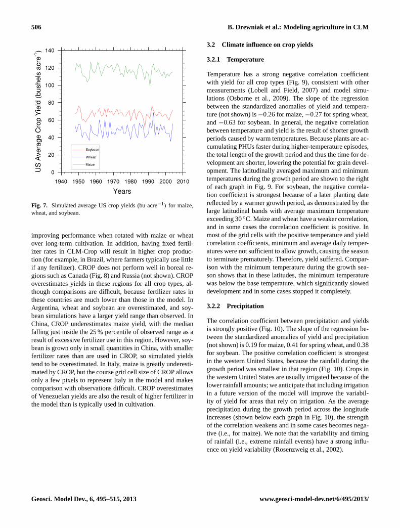
Global yield spreads compared with those of Monfredaet al. (2008) are shown in Fig. 8. In general, CROP medianyields are higher than observed yields for all crops, but yieldsvary regionally, mostly because the baseline growth model inCLM-Crop is representative of North America. Globally, thefull range of CROP yields for maize and wheat falls withinthe range of observed yields, although the spread of yieldsis quite large. Regionally this result is not always true. Yieldhas a large dependence on fertilizer rates, both in the modeland in the field. Fertilizer statistics from the Food and Agri-culture Organization (www.fao.org) reveal a large range in

Fig. 6. Simulated crop yields (bu acre−1) for (a) maize,(b) wheat,and(c) soybean.

fertilizer use, further increasing the difficulty of comparingCROP-simulated yields with observations.

Nevertheless, CROP-simulated median yields for most re-gions fall within the range of observed yields (i.e., maize inthe United States, Argentina, and China; wheat globally andin the United States, China, and Italy; and soybean in Brazil).Both soybean and spring wheat are overestimated in theUnited States; however, the range of maize and spring wheatyields simulated by CROP falls within the observed rangeof yields. Simulated soybean yields have a greater rangethan observations, demonstrating higher simulated variabil-ity in soybean yield across the United States, and 50 % ofthe soybean yields from CROP are higher than the observedyields (Fig. 8). In Argentina, the range of CROP-simulatedmaize production falls within the range of observations; inSouth Africa, the range of simulated maize yields has a largerspread than the observed value, and the median is muchhigher than the observed median yield.

Considering crop rotation in the model might improvethe yields in CLM, because soybean, as a legume, has theability to fix more nitrogen than do other crop types, thus


www.fao.org


Fig. 7. Simulated average US crop yields (bu acre−1) for maize,wheat, and soybean.

improving performance when rotated with maize or wheatover long-term cultivation. In addition, having fixed fertil-izer rates in CLM-Crop will result in higher crop produc-tion (for example, in Brazil, where farmers typically use littleif any fertilizer). CROP does not perform well in boreal re-gions such as Canada (Fig. 8) and Russia (not shown). CROPoverestimates yields in these regions for all crop types, al-though comparisons are difficult, because fertilizer rates inthese countries are much lower than those in the model. InArgentina, wheat and soybean are overestimated, and soy-bean simulations have a larger yield range than observed. InChina, CROP underestimates maize yield, with the medianfalling just inside the 25 % percentile of observed range as aresult of excessive fertilizer use in this region. However, soy-bean is grown only in small quantities in China, with smallerfertilizer rates than are used in CROP, so simulated yieldstend to be overestimated. In Italy, maize is greatly underesti-mated by CROP, but the course grid cell size of CROP allowsonly a few pixels to represent Italy in the model and makescomparison with observations difficult. CROP overestimatesof Venezuelan yields are also the result of higher fertilizer inthe model than is typically used in cultivation.

3.2 Climate influence on crop yields

3.2.1 Temperature

Temperature has a strong negative correlation coefficientwith yield for all crop types (Fig. 9), consistent with othermeasurements (Lobell and Field, 2007) and model simu-lations (Osborne et al., 2009). The slope of the regressionbetween the standardized anomalies of yield and tempera-ture (not shown) is−0.26 for maize,−0.27 for spring wheat,and−0.63 for soybean. In general, the negative correlationbetween temperature and yield is the result of shorter growthperiods caused by warm temperatures. Because plants are ac-cumulating PHUs faster during higher-temperature episodes,the total length of the growth period and thus the time for de-velopment are shorter, lowering the potential for grain devel-opment. The latitudinally averaged maximum and minimumtemperatures during the growth period are shown to the rightof each graph in Fig. 9. For soybean, the negative correla-tion coefficient is strongest because of a later planting datereflected by a warmer growth period, as demonstrated by thelarge latitudinal bands with average maximum temperatureexceeding 30◦C. Maize and wheat have a weaker correlation,and in some cases the correlation coefficient is positive. Inmost of the grid cells with the positive temperature and yieldcorrelation coefficients, minimum and average daily temper-atures were not sufficient to allow growth, causing the seasonto terminate prematurely. Therefore, yield suffered. Compar-ison with the minimum temperature during the growth sea-son shows that in these latitudes, the minimum temperaturewas below the base temperature, which significantly sloweddevelopment and in some cases stopped it completely.

3.2.2 Precipitation

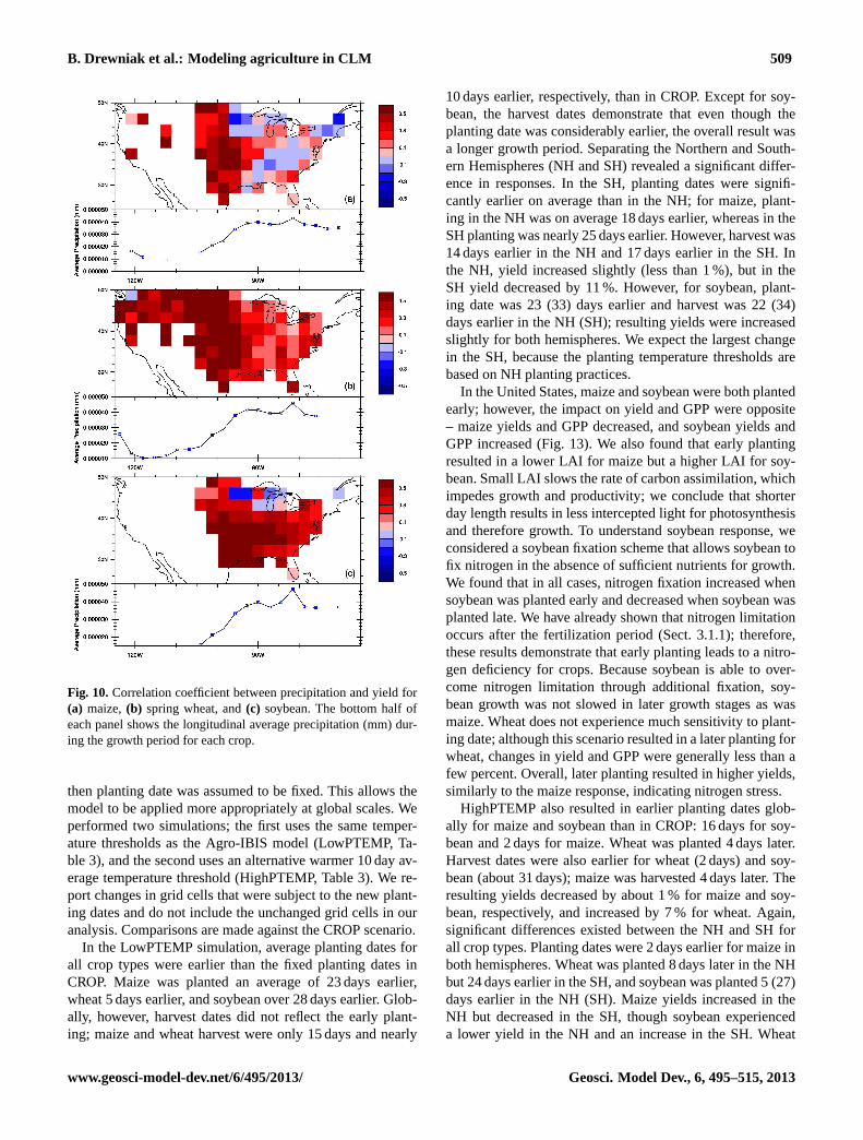
The correlation coefficient between precipitation and yieldsis strongly positive (Fig. 10). The slope of the regression be-tween the standardized anomalies of yield and precipitation(not shown) is 0.19 for maize, 0.41 for spring wheat, and 0.38for soybean. The positive correlation coefficient is strongestin the western United States, because the rainfall during thegrowth period was smallest in that region (Fig. 10). Crops inthe western United States are usually irrigated because of thelower rainfall amounts; we anticipate that including irrigationin a future version of the model will improve the variabil-ity of yield for areas that rely on irrigation. As the averageprecipitation during the growth period across the longitudeincreases (shown below each graph in Fig. 10), the strengthof the correlation weakens and in some cases becomes nega-tive (i.e., for maize). We note that the variability and timingof rainfall (i.e., extreme rainfall events) have a strong influ-ence on yield variability (Rosenzweig et al., 2002).



58

Corn Wheat Soy

0

50

100

150

200

All Countries

Yie

ld (b

u/ac

re)

CLMOBS

Corn Wheat Soy

0

50

100

150

200

United States

Yie

ld (b

u/ac

re)

Corn Wheat Soy

20

40

60

80

100

120

140

Argentina

Yie

ld (b

u/ac

re)

Corn Wheat Soy

20

40

60

80

100

Brazil

Yie

ld (b

u/ac

re)

Corn Wheat Soy

20

40

60

80

100

120

140

160

CanadaY

ield

(bu/

acre

)

Corn Wheat Soy

0

20

40

60

80

100

120

140

China

Yie

ld (b

u/ac

re)

Corn Wheat Soy

0

20

40

60

80

100

120

140

Italy

Yie

ld (b

u/ac

re)

Corn Wheat

20

40

60

80

100

120

140

South Africa

Yie

ld (b

u/ac

re)

Corn

30

40

50

60

70

Venezuela

Yie

ld (b

u/ac

re)

1015

Figure 8. CLM-Crop-simulated (black) and observed (gray; data from Monfreda et al., 1016

2008) yield (bu acre-1) for maize, wheat, and soybean of selected regions. 1017

1018

Fig. 8. CLM-Crop-simulated (black) and observed (gray; data from Monfreda et al., 2008) yields (bu acre−1) for maize, wheat, and soybeanof selected regions.

4 Case studies

4.1 Sensitivity of yield and GPP to residue management

To evaluate the impact of residue management on yield andproductivity, we tested two alternative residue returns (seeTable 3): a high residue return of 70 % (HIGHRES) and alow residue return of 10 % (LOWRES). The HIGHRES sce-nario would be typical of sustainable agriculture practices,minimizing the carbon removed from the field for alternativeuse and returning residue to the soil. The LOWRES scenario

represents a society with increased demand of biofuel fromagriculture residues. The amount of residue returned to thelitter pools affects decomposition and soil nutrients in thebelow-ground biogeochemistry, which will influence futuregrowth periods through nutrient availability. This should notbe confused with tillage practices, which are not representedin the model.

Increasing the amount of residue returned to the litter poolafter harvest has a positive influence on crop yield and GPP,globally. Likewise, decreasing the residue causes a decrease



Table 3.Parameter values for the baseline CLM-Crop simulation and the case studies.

Type of Change Scenario Maize Spring Wheat Soybean

Residue Management ( % non-grain residue returned to litterpool)

CROP 30 % 30 % 40 %

HIGHRES 70 % 70 % 70 %

LOWRES 10 % 10 % 10 %Planting Date (10 day runningaverage temperature thresholdfor planting)

CROP NA – fixed NA – fixed NA – fixed

HighPTEMP 22◦C 21◦C 17◦C

LowPTEMP 12◦C 11◦C 7◦C

Fig. 9. Correlation coefficient between temperature and yield for(a) maize,(b) spring wheat, and(c) soybean. The right half of eachpanel shows the latitudinal maximum and minimum temperatures(◦C) during the growth period for each crop.

in yield and GPP. Globally, for HIGHRES, yield increasedby 9, 8, and 5 % for maize, spring wheat, and soybean, re-spectively, compared to CROP. GPP likewise increased by 7,10, and 4 % for maize, spring wheat, and soybean, respec-tively. Figure 11 shows the percent change in yield and GPPfor all three crop types over the United States, although theMidwest Corn Belt has a larger increase in yield and GPP formaize and spring wheat than does the western United States.Drier conditions in the West could be responsible through aslowing of decomposition; incorporation of irrigation couldimprove results. For LOWRES, global yields and GPP de-clined by 4 % for maize and wheat and 7 % for soybean com-pared to CROP. The percent change is higher in the US Mid-west (Fig. 12), where farming is most concentrated. Thesesimulations indicate that below-ground processes do have astrong influence on above-ground processes, particularly re-lated to the turnover of carbon and nitrogen availability. Re-sults also demonstrate that high biofuel demands leading toremoval of crop residue for fuel use may result in a declinein crop productivity and degrade soil fertility over time. Wenote, however, that the nitrogen deficiency in the model mayexaggerate the results, especially for the low residue simula-tion where lack of nutrients affects future soil fertility.

4.2 Impact of variable planting date on yield and GPP

Because planting date is usually determined by farmers’choice, taking into account temperature, precipitation, andother conditions favorable for growth, we allowed the modelto determine a planting date adapted to climate conditionsfor the current year. In the Agro-IBIS model, planting dateis determined by 10 day running means of the average dailytemperature and the minimum daily temperature. In thiscase study, we adopted the Agro-IBIS approach to allowthe model to calculate a planting date by using the samemethods, but bounded by the earliest and latest plantingdates as reported by the Crop Calendar Dataset (Sacks et al.,2010). If the earliest and latest planting dates were unknown,



Fig. 10.Correlation coefficient between precipitation and yield for(a) maize,(b) spring wheat, and(c) soybean. The bottom half ofeach panel shows the longitudinal average precipitation (mm) dur-ing the growth period for each crop.

then planting date was assumed to be fixed. This allows themodel to be applied more appropriately at global scales. Weperformed two simulations; the first uses the same temper-ature thresholds as the Agro-IBIS model (LowPTEMP, Ta-ble 3), and the second uses an alternative warmer 10 day av-erage temperature threshold (HighPTEMP, Table 3). We re-port changes in grid cells that were subject to the new plant-ing dates and do not include the unchanged grid cells in ouranalysis. Comparisons are made against the CROP scenario.

In the LowPTEMP simulation, average planting dates forall crop types were earlier than the fixed planting dates inCROP. Maize was planted an average of 23 days earlier,wheat 5 days earlier, and soybean over 28 days earlier. Glob-ally, however, harvest dates did not reflect the early plant-ing; maize and wheat harvest were only 15 days and nearly

10 days earlier, respectively, than in CROP. Except for soy-bean, the harvest dates demonstrate that even though theplanting date was considerably earlier, the overall result wasa longer growth period. Separating the Northern and South-ern Hemispheres (NH and SH) revealed a significant differ-ence in responses. In the SH, planting dates were signifi-cantly earlier on average than in the NH; for maize, plant-ing in the NH was on average 18 days earlier, whereas in theSH planting was nearly 25 days earlier. However, harvest was14 days earlier in the NH and 17 days earlier in the SH. Inthe NH, yield increased slightly (less than 1 %), but in theSH yield decreased by 11 %. However, for soybean, plant-ing date was 23 (33) days earlier and harvest was 22 (34)days earlier in the NH (SH); resulting yields were increasedslightly for both hemispheres. We expect the largest changein the SH, because the planting temperature thresholds arebased on NH planting practices.

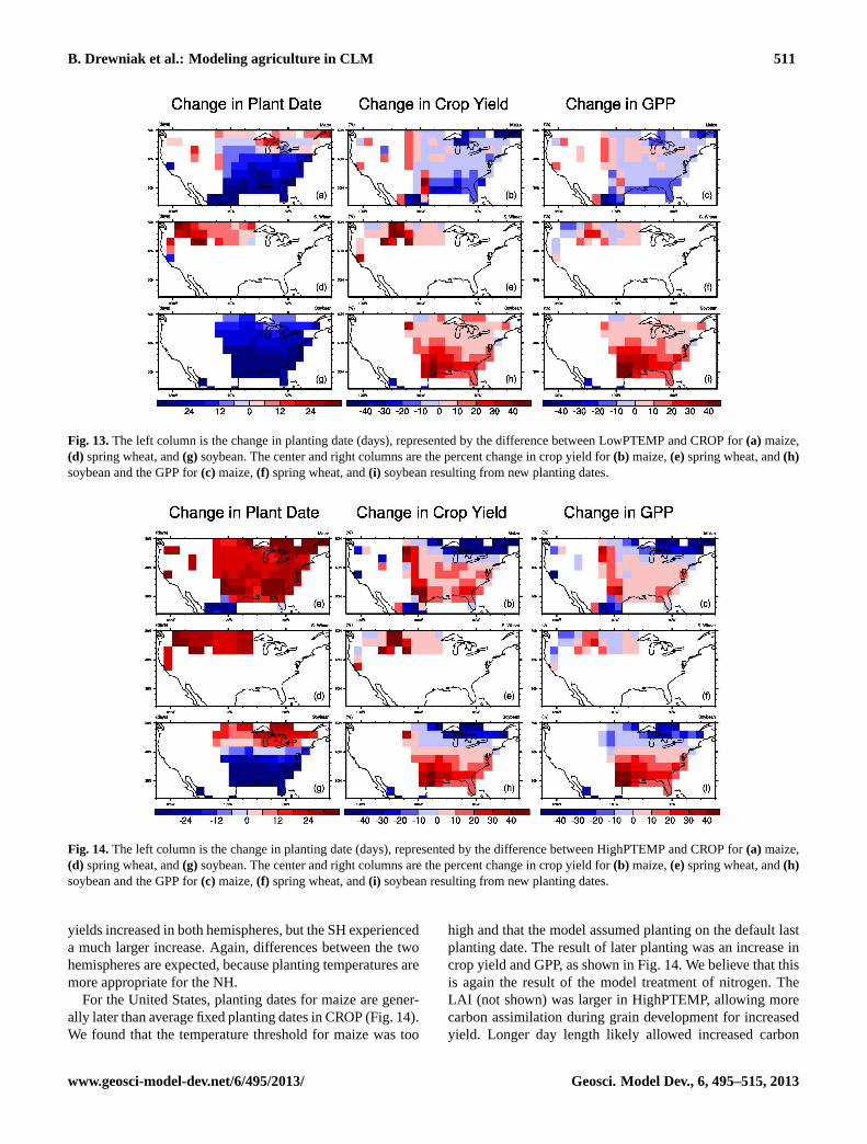
In the United States, maize and soybean were both plantedearly; however, the impact on yield and GPP were opposite– maize yields and GPP decreased, and soybean yields andGPP increased (Fig. 13). We also found that early plantingresulted in a lower LAI for maize but a higher LAI for soy-bean. Small LAI slows the rate of carbon assimilation, whichimpedes growth and productivity; we conclude that shorterday length results in less intercepted light for photosynthesisand therefore growth. To understand soybean response, weconsidered a soybean fixation scheme that allows soybean tofix nitrogen in the absence of sufficient nutrients for growth.We found that in all cases, nitrogen fixation increased whensoybean was planted early and decreased when soybean wasplanted late. We have already shown that nitrogen limitationoccurs after the fertilization period (Sect. 3.1.1); therefore,these results demonstrate that early planting leads to a nitro-gen deficiency for crops. Because soybean is able to over-come nitrogen limitation through additional fixation, soy-bean growth was not slowed in later growth stages as wasmaize. Wheat does not experience much sensitivity to plant-ing date; although this scenario resulted in a later planting forwheat, changes in yield and GPP were generally less than afew percent. Overall, later planting resulted in higher yields,similarly to the maize response, indicating nitrogen stress.

HighPTEMP also resulted in earlier planting dates glob-ally for maize and soybean than in CROP: 16 days for soy-bean and 2 days for maize. Wheat was planted 4 days later.Harvest dates were also earlier for wheat (2 days) and soy-bean (about 31 days); maize was harvested 4 days later. Theresulting yields decreased by about 1 % for maize and soy-bean, respectively, and increased by 7 % for wheat. Again,significant differences existed between the NH and SH forall crop types. Planting dates were 2 days earlier for maize inboth hemispheres. Wheat was planted 8 days later in the NHbut 24 days earlier in the SH, and soybean was planted 5 (27)days earlier in the NH (SH). Maize yields increased in theNH but decreased in the SH, though soybean experienceda lower yield in the NH and an increase in the SH. Wheat



Fig. 11.The percent change in yield (left column) and GPP (right column) for(a, b) maize,(c, d) spring wheat, and(e, f) soybean from a70 % residue return management practice (HIGHRES).

Fig. 12.The percent change in yield (left column) and GPP (right column) for(a, b) maize,(c, d) spring wheat, and(e, f) soybean from a10 % residue return management practice (LOWRES).



Fig. 13.The left column is the change in planting date (days), represented by the difference between LowPTEMP and CROP for(a) maize,(d) spring wheat, and(g) soybean. The center and right columns are the percent change in crop yield for(b) maize,(e)spring wheat, and(h)soybean and the GPP for(c) maize,(f) spring wheat, and(i) soybean resulting from new planting dates.

Fig. 14.The left column is the change in planting date (days), represented by the difference between HighPTEMP and CROP for(a) maize,(d) spring wheat, and(g) soybean. The center and right columns are the percent change in crop yield for(b) maize,(e)spring wheat, and(h)soybean and the GPP for(c) maize,(f) spring wheat, and(i) soybean resulting from new planting dates.

yields increased in both hemispheres, but the SH experienceda much larger increase. Again, differences between the twohemispheres are expected, because planting temperatures aremore appropriate for the NH.

For the United States, planting dates for maize are gener-ally later than average fixed planting dates in CROP (Fig. 14).We found that the temperature threshold for maize was too

high and that the model assumed planting on the default lastplanting date. The result of later planting was an increase incrop yield and GPP, as shown in Fig. 14. We believe that thisis again the result of the model treatment of nitrogen. TheLAI (not shown) was larger in HighPTEMP, allowing morecarbon assimilation during grain development for increasedyield. Longer day length likely allowed increased carbon



assimilation during the fertilizer application period, whichbenefited the crop throughout the growth period. Wheat wasplanted slightly later, but, like the LowPTEMP condition, itshowed little sensitivity to planting date other than a slightincrease in yields in most areas (Fig. 14). Soybean was stillplanted early in the southern United States but was plantedlater in the northern United States. The resulting change inyield is still an increase in the South, but a decrease in yieldoccurs with later planting. Soybean fixation (not shown) in-creased in the South but decreased in the North (where de-creases in yield occurred). Most of the decreases in the Northwere the result of insufficient PHU accumulation to reachmaturity prior to the onset of the cool season resulting in anautomatic harvest.

5 Discussion

Cultivation has serious effects on the terrestrial carbon cycle,and the consequences of land management for carbon fluxeshave only recently been included in earlier land surface mod-eling within the CLM framework (Levis et al., 2012). Pre-vious versions of CLM had either a crude representationof crops or omitted many traits that are important, such asfertilizer, soybean fixation, and retranslocation. CLM-Crop,which can assess the impacts of several crop types on bio-geochemical cycles, has been evaluated for the United Statesby using field measurement data for maize and soybean sys-tems. Although the model does well in representing appro-priate responses for agriculture systems, including improv-ing the global simulated GPP fluxes, remaining inconsisten-cies include decreased GPP for maize during the middle ofthe growth period and overestimated yields for soybean andwheat. Improvements to the nitrogen scheme in the model,including a more complex fertilizer application and denitri-fication factor, might help to correct disagreements betweenthe model output and observations.

CLM-Crop simulations agree with other crop models inpredicting a negative correlation between yield and temper-ature and a positive correlation between yield and precipita-tion. This has important implications, indicating that as cli-mate shifts, crop yields might be expected to decline. Thisresult could be amplified when extreme weather events in-cluding drought, heat waves, and heavy precipitation eventsare taken into account, as predicted by the IntergovernmentalPanel on Climate Change (Meehl et al., 2007).

Residue management can have strong implications foryield and productivity, as shown by CLM-Crop. Increasingthe amount of plant harvested for use as animal bedding,feed, or biomass fuel can influence below-ground biogeo-chemistry cycling, which impacts soil quality and thereforefuture yields. Because few statistics on residue managementexist, application of this management practice is difficult toimplement; however, the sensitivity of yield to the amount ofresidue left on the field as simulated by CLM-Crop demon-

strates that residue is an important consideration for sustain-able cultivation. As below-ground carbon and nitrogen cy-cling are improved in CLM, dependence of crop productiv-ity on nutrient availability from residue management shoulddecrease, although sensitivity to decomposition and turnoverwill still remain.

Both the HighPTEMP and LowPTEMP simulations showthat the model has a high sensitivity to the planting date, be-cause of the influence of planting date on timing of growth.The most important development period during crop growthseems to be in the early stages, when assimilated carbon andnitrogen will influence the remainder of the growth period,particularly because the amount of carbon allocated to leavesdecreases with time. Even more notably, the nitrogen cyclingin the model has significant influence on crop development.Availability of nitrogen during crucial stages of growth sig-nificantly affects how a plant prospers. Improvements in thenitrogen cycling and coupling in the model should enhancenitrogen availability and perhaps limit this sensitivity.

Expanding the model to incorporate other managementpractices (tillage, irrigation, etc.) is important for futuremodel development. Although the crop representation inCLM-Crop is flexible enough for expansion to a global scale,rigorous testing is needed to ensure that crop behavior isconsistent with regional observations. Other additions to theCLM-Crop model should improve the carbon cycling repre-sentation. The current CLM framework allows natural veg-etation to change with time; however, managed croplandsas they are treated in this model cannot expand or contract.Using historical vegetation data to create a transient vegeta-tion data set with appropriate deforestation/reforestation andgrassland removal rates related to the growth or abandon-ment of cultivated land use could improve the performanceof CLM-Crop. In addition, our parameter calibration is fo-cused on crop species grown in the United States; expand-ing these parameters to capture other cultivars grown morebroadly would improve the model’s ability to capture globalcrop productivity. One example is to use fertilizer data setsto establish spatial fertilizer application by crop type, such asthat developed by Potter et al. (2010).

While the improvements to CLM showed better agreementwith above-ground cycling, we have not considered below-ground carbon, which is an integral component for properconsideration of the full carbon cycle in an Earth systemmodel. Further research is needed to understand the impor-tance of agro-ecosystems on soil carbon. Soil organic car-bon loss can vary greatly, depending on management prac-tices, and including actions such as fertilizer and residuemanagement in modeling studies is important for simulatingeffects on carbon storage. Incorporating crop representationinto CLM is the first step toward evaluating the impacts ofland management within an Earth system model.



Acknowledgements.We would like to extend our thanks toSam Levis for his helpful discussions and guidance with modeldevelopment. Our gratitude also goes to Bill Sacks for makingthe Crop Calendar Dataset available for use as model input. Thework of Drewniak, Song, Prell, Kotamarthi, and Jacob at ArgonneNational Laboratory was supported by the US Department ofEnergy, Office of Science, under contract DE-AC02-06CH11357.Numerical simulations were performed with resources providedby the National Energy Research Scientific Computing Center,supported by the Office of Science and US Department of EnergyContract No. DE-AC02-05CH11231.

Edited by: M.-H. Lo

References

Amanullah, M. J. H., Nawab, K., and Ali, A.: Response of SpecificLeaf Area (SLA), Leaf Area Index (LAI) and Leaf Area Ratio(LAR) of maize (Zea mays L.) to plant density, rate and timingof nitrogen application, World Appl. Sci. J., 2, 235–243, 2007.

Amos, B. and Walters, D. T.: Maize root biomass and net rhizode-posited carbon, Soil Sci. Soc. Am. J., 70, 1489–1503, 2006.

Araki, H. and Iijima, M.: Deep rooting in winter wheat: rootingnodes of deep roots in two cultivars with deep and shallow rootsystem, Plant Prod. Sci., 4, 215–219, 2001.

Barbottin, A., Lecomte, C., Bouchard, C., and Jeuffroy, M.-H.: Ni-trogen remobilization during grain filling in wheat: Genotypicand environmental effects, Crop Sci., 45, 1141–1150, 2005.

Batjes, N. H.: ISRIC-WISE harmonized global soil profile dataset(Ver. 3.1). Report 2008/02, ISRIC – World Soil Information, Wa-geningen, 2008.

Blanco-Canqui, H. and Lal, R.: No-tillage and soil-profile carbonsequestration: an on-farm assessment, Soil Water Manag. Con-servation, 72, 693–701, 2008.

Bonan, G. B., Levis, S., Kergoat, L., and Oleson, K. W.: Land-scapes as patches of plant functional types: An integrating con-cept for climate and ecosystem models, Global Biogeochem. Cy.,16, 1021,doi:10.1029/2000GB001360, 2002.

Bondeau, A., Smith, P. C., Zaehle, S., Schaphoff, S., Lucht, W.,Cramer, W., Gerten, D., Lotze-Campen, H., Mullers, C., Reich-stein, M., and Smith, B.: Modeling the role of agriculture for the20th century global terrestrial carbon balance, Global ChangeBiol., 13, 679–706, 2007.

Crawford, T. W., Rendig, V. V., and Broadent, F. E.: Sources, fluxes,and sinks of nitrogen during early reproductive growth of maize(Zea mays L.), Plant Physiol., 70, 1645–1660, 1982.

Diffenbaugh, N. S.: Influence of modern land cover on the climateof the United States, Climate Dynam., 33, 945–958, 2009.

Dou, F. and Hans, F. M.: Tillage and nitrogen effects on soil organicmatter fractions in wheat-based systems, Soil Sci. Soc. Am. J.,70, 1896–1905, 2006.

Fargione, J., Hill, J., Tilman, D., Polasky, S., and Hawthorne, P.:Land clearing and the biofuel carbon debt, Science, 319, 1235–1238, 2008.

Fischer, G., Shah, M., Tubiello, F. N., and van Velhuizen, H.: Socio-economic and climate change impacts on agriculture: an inte-grated assessment, 1990-2080, Philos. T. R. SOC. A, 360, 2067–2083, 2005.

Gallais, A., Coque, M. Quillere, I., Prioul, J., and Hirel, B.: Model-ing postsilking nitrogen fluxes in maize (Zea mays) using15N-labeling field experiments, New Phytol., 172, 696–707, 2006.

Gallais, A., Coque, M., Gouis, J. L., Prioul, J. L., Hirel, B., andQuillere, I.: Estimating the proportion of nitrogen remobilizationand of postsilking nitrogen uptake allocated to maize kernels byNitrogen-15 labeling, Crop Sci., 47, 685–693, 2007.

Garay, A. F. and Wilhelm W. W.: Root system characteristics of twosoybean isolines undergoing water stress conditions, AgronomyJ., 75, 973–977, 1983.

Gibbs, H. K., Johnston, M., Foley, J. A., Holloway, T., Mon-freda, C., Ramankutty, N., and Zaks, D.: Carbon payback timesfor crop-based biofuel expansion in the tropics: the effects ofchanging yield and technology, Environ. Res. Lett., 3, 034001,doi:10.1088/1748-9326/3/3/034001, 2008.

Hooker, B. A., Morris, T. F., Peters, R., and Cardon, Z. G.: Long-term effects of tillage and corn stalk return on soil carbon dy-namics, Soil Sci. Soc. Am. J., 69, 188–196, 2005.

Huggins, D. R., Allmaras, R. R., Clapp, C. E., Lamb, J. A., andRandall, G. W.: Corn-soybean sequence and tillage effects on soilcarbon dynamics and storage, Soil Sci. Soc. Am. J., 71, 145–154,2007.

Hurtt, G. C., Frolking, S., Fearon, M. G., Moore, B., Shevliakova,E., Malyshev, S., Pacala, S. W., and Houghton, R. A.: The un-derpinnings of land-use history: three centuries of global grid-ded land-use transitions, wood harvest activity, and resulting sec-ondary lands, Global Change Biol., 12, 1208–1229, 2006.

Jobbagy, E. G. and Jackson, R. B.: The distribution of soil nutrientswith depth: Global patterns and the imprint of plants, Biogeo-chemistry, 53, 51–77, 2001.

Kalnay, E., Kanamitsu, M., Kistler, R., Collins, W., Deaven, D.,Gandin, L., Iredell, M., Saha, S., White, G., Woolen, J., Zhu, Y.,Chelliah, M., Ebisuzaki, W., Higgins, W., Janowiak, J., Mo, K.C., Ropelewski, C., Wang, J., Leetmaa, A., Reynolds, R., Jenne,R., and Joseph, D.: The NCEP/NCAR 40-year reanalysis project,Bull. Amer. Meteor. Soc., 77, 437–470, 1996.

Khan, S. A., Mulvaney, R. L., Ellsworth, T. R., and Boast, C. W.:The myth of nitrogen fertilization for soil carbon sequestration,J. Environ. Qual, 36, 1821–1832, 2007.

Kim, H., Kim, S., and Dale, B. E.: Biofuels, land use change, andgreenhouse gas emissions: Some unexplored variables, Environ.Sci. Technol., 43, 961–967, 2009.

Kucharik, C. J.: Evaluation of a process-based agro-ecosystemmodel (Agro-IBIS) across the US Corn Belt: Simulations of theinterannual variability in maize yield, Earth Interact., 7, 1–33,2003.

Kucharik, C. J.: Contributions of planting date trends to increasedmaize yields in the Central United States, Agronomy J., 100,328–336, 2008.

Kucharik, C. J. and Brye, K. R.: Integrated BIosphere Simulator(IBIS) Yield and Nitrate Loss Predictions for Wisconsin MaizeReceiving Varied Amounts of Nitrogen Fertilizer, J. Environ.Qual., 32, 247–268, 2003.

Kucharik, C. J. and Twine, T. E.: Residue, respiration, and residuals:Evaluation of a dynamic agroecosystem model using eddy fluxmeasurements and biometric data, Agr. Forest Meteorol., 146,134–158, 2007.

Leff, B., Ramankutty, N., and Foley, J. A.: Geographic distributionof major crops across the world, Global Biogeochem. Cy., 18,


http://dx.doi.org/10.1029/2000GB001360

http://dx.doi.org/10.1088/1748-9326/3/3/034001


GB1009,doi:10.1029/2003GB002108, 2004.Levis, S., Bonan, G. B., Kluzek, E., Thornton, P. E., Jones, A.,

Sacks, W. J., Kucharik, C. J.: Interactive Crop Management in theCommunity Earth System Model (CESM1): seasonal influenceson land-atmosphere fluxes, J. Climate, 25,doi:10.1175/JCLI-D-11-00446.1, 2012.

Lobell, D. B., Bala, G., and Duffy, P. B.: Biogeophysical impacts ofcropland management changes on climate, Geophys. Res. Lett.,33, L06708,doi:10.1029/2005GL025492, 2006.

Lobell, D. B. and Field, C. B.: Global scale climate-crop yield rela-tionships and the impacts of recent warming, Environ. Res. Lett.,2, 014002,doi:10.1088/1748-9326/2/1/014002, 2007.

Lobell, D. B., Schlenker, W., and Costa-Roberts, J.: Climate trendsand global crop production since 1980, Science, 333, 616–620,2011.

Mayaki, W. C., Reare, I. D., and Stone L. R.: Top and root growth ofirrigated and non-irrigated soybean, Crop Sci., 16, 92–94, 1976.

Meehl, G. A., Stocker, T. F., Collins, W. D., Friedlingstein, P., Gaye,A. T., Gregory, J. M., Kitoh, A., Knutti, R., Murphy, J. M., Noda,A., Raper, S. C. B., Watterson, I. G., Weaver, A. J., and Zhao, Z.-C.: Global Climate Projections. In: Climate Change 2007: ThePhysical Science Basis, in: Contribution of Working Group I tothe Fourth Assessment Report of the Intergovernmental Panel onClimate Change, edited by: Solomon, S., Qin, D., Manning, M.,Chen, Z., Marquis, M., Averyt, K. B., Tignor, M., and Miller,H. L., Cambridge University Press, Cambridge, United Kingdomand New York, NY, USA, 747–845, 2007.

Monfreda, C., Ramankutty, N., and Foley, J. A.: Farming the planet:2. Geographic distribution of crop areas, yields, physiologicaltypes, and net primary production in the year 2000, Global Bio-geochem. Cy., 22, GB1022,doi:10.1029/2007GB002947, 2008.

Neitsch, S. L., Arnold, J. G., Kiniry, J. R., and Williams J. R.: Soiland Water Assessment Tool, Theoretical Documentation: Ver-sion 2005. Temple, TX. USDA Agricultural Research Serviceand Texas A&M Blackland Research Center, 2005.

New, M., Hulme, M., and Jones, P. D.: Representing Twentieth-Century Space-Time Climate Variability. Part I: Development ofa 1961–90 Mean Monthly Terrestrial Climatology, J. Climate,12, 829-856, 1999.

Oleson, K. W., Dai, Y., Bonan, G., Bosilovich, M., Dickinson,R., Dirmeyer, P., Hoffman, F., Houser, P., Levis, S., Niu, G.-Y., Thornton, P., Vertenstein, M., Yang, Z.-L., and Zeng, X.:Technical Description of the Community Land Model (CLM).NCAR/TN-461+STR, National Center for Atmospheric Re-search, Boulder, Colorado, 2004.

Oleson, K. W., Niu, G.-Y., Yang, Z.-L., Lawrence, D. M., Thornton,P. E., Lawrence, P. J., Stockli, R., Dickinson, R. E., Bonan, G. B.,Levis, S., Dai, A., and Qian, T.: Improvements to the CommunityLand Model and their impact on the hydrological cycle, J. Geo-phys. Res., 113, G01021,doi:10.1029/2007JG000563, 2008.

Osborne, T. M., Lawrence, D. M., Challinor, A. J., Slingo, J. M.,and Wheeler, T. R.: Development and assessment of a coupledcrop-climate model, Global Change Biol., 13, 169–183, 2007.

Osborne, T., Slingo, J., Lawrence, D., and Wheeler, T.: Examiningthe interaction of growing crops with local climate using a cou-pled crop-climate model, J. Climate, 22, 1393–1411, 2009.

Papale, D. and Valentini, R.: A new assessment of European forestscarbon exchanges by eddy fluxes and artificial neural networkspatialization, Global Change Biol., 9, 525–535, 2003.

Parry, M. L., Rosenzweig, C., Iglesias, A., Livermore, M., and Fis-cher, G: Effects of climate change on global food production un-der SRES emissions and socio-economic scenarios, Global Env-iron. Change, 14, 53–67, 2004.

Pollmer, W. G., Eberhard, D., Klein, D., and Dhillon, B. S.: Geneticcontrol of nitrogen uptake and translocation in maize, Crop Sci.,19, 82–86, 1979.

Potter, P., Ramankutty, N., Bennett, E. M., and Donner, S.D.: Characterizing the spatial patterns of global fertilizer ap-plication and manure production, Earth Interact., 14, 1–22,doi:10.1175/2009EI288.1, 2010.

Reichstein, M., Falge, E., Baldocchi, D., Papale, D., Aubinet,M., Berbigier, P., Bernhofer, C., Buchmann, N., Gilmanov, T.,Grainer, A., Grunwald, T., Havrankova, K., Ilvesniemi, H.,Janous D., Knohl, A., Laurila, T., Lohila, A., Loustau, D., Mat-teucci, G., Meyers, T., Miglietta, F., Ourcival, J.-M., Pumpanen,J., Rambal, S., Rotenberg, E., Sanz, M., Tenhunen, J., Seufert, G.,Vaccari, F., Vesala, T., Yakir, D., and Valentini, R.: On the sep-aration of net ecosystem exchange into assimilation and ecosys-tem respiration: review and improved algorithm, Global ChangeBiol., 11, 1424–1439, 2005.

Rosenzweig, C., Tubiello, F. N., Goldberg, R, Mills, E., and Bloom-field, J.: Increased crop damage in the US from excess precipi-tation under climate change, Global Environ. Change, 12, 197–202, 2002.

Sacks, W. J., Deryng, D., Foley, J. A., and Ramankutty, N.: Cropplanting dates: an analysis of global patterns, Global Ecol. Bio-geogr., 19, 607–620, doi: 10.1111/j.1466-8238.2010.00551.x,2010.

Schlenker, W. and Roberts, M. J.: Nonlinear temperature effects in-dicate severe damages to US crop yields under climate change,Proc. National Academy Sci., 106, 15594–15598, 2009.

Searchinger, T., Heimlick, R., Houghton, R. A., Dong, F., Elobeid,A., Fabiosa, J., Tokgoz, S., Hayes, D., and Yu, T.-H.: Use of UScroplands for biofuels increases greenhouse gases through emis-sions from land use change, Science, 319, 1238–1240, 2008.

Simpson, R. J., Lambers, H., and Dalling, M. J.: Nitrogen redis-tribution during grain growth in wheat (Triticum avestivum L.),Plant Physiol., 71, 7–14, 1983.

Smith, P. C., De Noblet-Decoudre, N., Ciais, P., Peylin, P., Viovy,N., Meurdesoif, Y., and Bondeau, A.: European-wide simula-tions of croplands using an improved terrestrial biosphere model:Phenology and productivity, J. Geophys. Res., 115, G01014,doi:10.1029/2008JG000800, 2010.

Stockli, R., Lawrence, D. M., Niu, G.-Y., Oleson, K. W., Thorn-ton, P. E., Yang, Z.-L., Bonan, G. B., Denning, A. S.,and Running, S. W.: Use of FLUXNET in the CommunityLand Model development, J. Geophys. Res., 113, G01025,doi:10.1029/2007JG000562, 2008.

Ta, C. T. and Weiland, R. T.: Nitrogen partitioning in maize duringear development, Crop Sci., 32, 443–451, 1992.

Tang, J. Y., Riley, W. J., Koven, C. D., and Subin, Z. M.: CLM4-BeTR, a generic biogeochemical transport and reaction mod-ule for CLM4: model development, evaluation, and application,Geosci. Model Dev., 6, 127–140,doi:10.5194/gmd-6-127-2013,2013.

Tardieu, F., Granier, C., and Muller, B.: Modelling leaf expansionin a fluctuating environment: are changes in specific leaf areaa consequence of changes in expansion rate?, New Phytologist,


http://dx.doi.org/10.1029/2003GB002108

http://dx.doi.org/10.1175/JCLI-D-11-00446.1

http://dx.doi.org/10.1175/JCLI-D-11-00446.1

http://dx.doi.org/10.1029/2005GL025492

http://dx.doi.org/10.1088/1748-9326/2/1/014002

http://dx.doi.org/10.1029/2007GB002947

http://dx.doi.org/10.1029/2007JG000563

http://dx.doi.org/10.1175/2009EI288.1

http://dx.doi.org/10.1029/2008JG000800

http://dx.doi.org/10.1029/2007JG000562

http://dx.doi.org/10.5194/gmd-6-127-2013


143, 33–43, 1999.Thornton, P. E. and Rosenbloom, N.: Ecosystem model spin-up: es-

timating steady state conditions in a coupled terrestrial carbonand nitrogen cycle model, Ecol. Model., 189, 25–48, 2005.

Thornton, P. E. and Zimmerman, N. E.: An improved canopy inte-gration scheme for a land surface model with prognostic canopystructure, J. Climate, 20, 3902–3923, 2007.

Urban, D., Roberts, M. J., Schlenker, W., and Lobell, D. B.: Pro-jected temperature changes indicate significant increase in in-terannual variability of US maize yields, Climatic Change, 112,525–533, 2012.

West, T. O. and Post, W. M.: Soil organic carbon sequestration ratesby tillage and crop rotation: a global data analysis, Soil Sci. Soc.Am. J., 66, 1930–1946, 2002.

Zhao, M., Heinsch, F. A., Nemani, R. R., and Running, S. W.: Im-provements of the MODIS terrestrial gross and net primary pro-duction global data set, Remote Sens. Environ., 95, 164–176,2005.


Modeling agriculture in the Community Land Model. Drewniak1, J. Song2, J. Prell1, V. R. Kotamarthi1,...

Documents

Transcript of Modeling agriculture in the Community Land Model. Drewniak1, J. Song2, J. Prell1, V. R. Kotamarthi1,...