Modeling a Million-Node Slim Fly Network Using ParallelDiscrete-Event Simulation

Noah Wolfe, Christopher CarothersRensselaer Polytechnic Institute

110 8th StTroy, NY

wolfen,chrisc@rpi.edu

Misbah Mubarak, Robert Ross,Philip Carns

Argonne National Laboratory9700 South Cass Avenue

Lemont, IL 60439mmubarak,rross,carns@mcs.anl.gov

ABSTRACTAs supercomputers close in on exascale performance, the in-creased number of processors and processing power trans-lates to an increased demand on the underlying networkinterconnect. The Slim Fly network topology, a new low-diameter and low-latency interconnection network, is gain-ing interest as one possible solution for next-generation su-percomputing interconnect systems. In this paper, we presenta high-fidelity Slim Fly flit-level model leveraging the Rens-selaer Optimistic Simulation System (ROSS) and Co-Designof Exascale Storage (CODES) frameworks. We validate ourSlim Fly model with the Kathareios et al. Slim Fly modelresults provided at moderately sized network scales. Wefurther scale the model size up to n unprecedented 1 mil-lion compute nodes; and through visualization of networksimulation metrics such as link bandwidth, packet latency,and port occupancy, we get an insight into the network be-havior at the million-node scale. We also show linear strongscaling of the Slim Fly model on an Intel cluster achievinga peak event rate of 36 million events per second using 128MPI tasks to process 7 billion events. Detailed analysis ofthe underlying discrete-event simulation performance showshow the million-node Slim Fly model simulation executes in198 seconds on the Intel cluster.

CCS Concepts•Computing methodologies → Discrete-event simu-lation; Model verification and validation; Parallel al-gorithms; •Networks → Network simulations;

KeywordsSlim Fly; Network topologies; Parallel discrete event simu-lation; Interconnection networks

Publication rights licensed to ACM. ACM acknowledges that this contribution wasauthored or co-authored by an employee, contractor or affiliate of the United Statesgovernment. As such, the Government retains a nonexclusive, royalty-free right topublish or reproduce this article, or to allow others to do so, for Government purposesonly.

SIGSIM-PADS ’16, May 15 - 18, 2016, Banff, AB, Canadac© 2016 Copyright held by the owner/author(s). Publication rights licensed to ACM.

ACM ISBN 978-1-4503-3742-7/16/05. . . $15.00

DOI: http://dx.doi.org/10.1145/2901378.2901389

1. INTRODUCTIONPerformance of interconnection networks is integral to

large-scale computing systems. Current HPC systems havethousands of compute nodes; for example, the Mira BlueGene/Q system at Argonne has 49,152 compute nodes [23].Some of the future pre-exascale machines, such as Aurorato be deployed at Argonne National Laboratory, will haveover 50,000 compute nodes [13]. The ability of the inter-connection network to transfer data efficiently is essentialto the successful implementation and deployment of suchlarge-scale HPC systems. There is a trade-off of latency,cost, and diameter among the potential network topologiesthat currently exist. One topology that meets all three met-rics is Slim Fly, as proposed by Besta and Hoefler [4]. Highbandwidth, low latency, low cost, and a low network diam-eter are all properties of the Slim Fly network that make ita solid option as an interconnection network for large-scalecomputing systems.

In this paper, we present a highly efficient and detailedmodel of the Slim Fly network topology using massively par-allel discrete-event simulation. Validating against the SlimFly simulator by Besta and Hoefler [4], our Slim Fly modelis capable of performing minimal, non-minimal, and adap-tive routing under uniform random and worst-case trafficworkloads. Our model is also capable of large-scale networkmodeling; and in this paper, we execute a million-node SlimFly network on the RSA Intel cluster at Rensselaer Polytech-nic Institute (RPI) Center for Computation Innovations. Inaddition, our model has been implemented to execute underoptimistic event scheduling using reverse computation andachieves 36 million events per second while maintaining 99%efficiency. This level of performance establishes our Slim Flymodel as a useful tool that will give network designers thecapability to analyze different design options of Slim Flynetworks.

The main contributions of this paper are as follows.

• A Rensselaer Optimistic Simulation System (ROSS)parallel discrete event Slim Fly network model thatcan simulate large-scale Slim Fly networks at a detailedfidelity and provide insight into network behavior byrecording detailed metrics at this scale. The Slim Flymodel is also shown to be in close agreement with theKathareios et al. Slim Fly network simulator [14].

• We simulate and provide a detailed visual analysis ofa Slim Fly network at a scale of 74,000 nodes, inspiredby the Argonne Aurora supercomputer.

• This paper also models the largest discrete-event SlimFly network to date at just over 1 million nodes andcrossing the 7 billion committed events mark.

• In terms of the simulation performance itself, a strong-scaling study of our simulation demonstrates that ourSlim Fly model is highly scalable and can achieve anevent rate of 43 million events per second on 16 nodes,128 processes of the Intel cluster at RPI [8]

The remainder of the paper is organized as follows. Sec-tion 2 provides the network simulation design in terms ofthe topology, routing algorithms and flow control. We alsodescribe the details of the discrete event simulation imple-mentation. Section 3 presents the validation experiments.Section 4 describes the network and discrete-event simula-tion performance results. Section 5 discusses related work,and Section 6 summarizes our conclusions and briefly dis-cusses future work.

2. SLIM FLY NETWORK MODELIn this section, we describe the simulation design of the

Slim Fly topology as well as its implementation in the formof a discrete event simulation.

Table 1: Descriptions of symbols used

Topic Symbol Description

p Nodes connected to a routerNr Total routers in network (Nr = 2q2)

SF Nn Total nodes in network (Nn = Nr ∗ p)k′ Router network radixk Router radix (k = k′ + p)q Prime power

CODES/ LP Logical Process (simulated entity)ROSS PE Processing element (MPI rank)

2.1 Slim Fly TopologyIntroduced by Besta and Hoefler [4], the Slim Fly consists

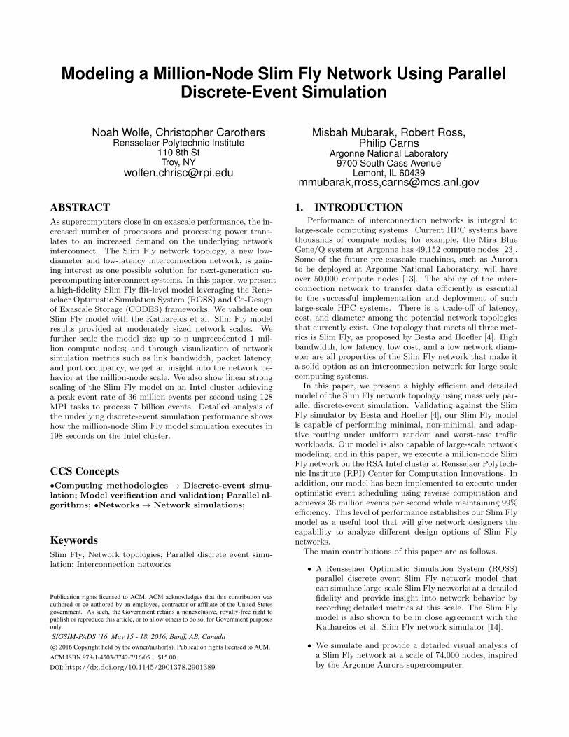
of groups of routers with direct connections to other routersin the network similar in nature to the dragonfly intercon-nect topology. Each router has a degree of local connectivityto other routers in its local group and a global degree of con-nectivity to routers in other groups. Unlike the dragonflytopology, however, the Slim Fly does not have fully con-nected router groups. Within each group, each router hasonly a subset of intragroup connections governed by one oftwo specific equations based on the router’s subgraph mem-bership. Furthermore, all router groups are split into twosubgraphs. Each router possesses global intergroup connec-tions only to routers within the opposite subgraph, forminga bipartite graph between the two subgraphs. These globalconnections are also constructed according to a third equa-tion [4]. Figure 1. shows a simple example of the describedstructure and layout of the Slim Fly topology.

An important feature of the Slim Fly topology is that itsgraphs are constructed to guarantee a given maximum diam-eter. One example set of graphs, which we use in this paper,is the collection of diameter 2 graphs introduced by McKayet al. [16], called MMS graphs. MMS graphs guarantee amaximum of 2 hops when traversing the network layer andbecause they approach the Moore bound [18], these graphs

…" …" …"…"

…" …" …" …"

routers" nodes" node"connec,ons" local"connec,ons" global"connec,ons"

Figure 1: General structure and layout of MMS Slim Flygraphs. Global connections between subgraphs have beengeneralized for clarity. There are no intergroup connectionswithin the same subgraph. Each router contains one globalconnection to one router in each of the q-many router groupsin the opposing subgraph.

constitute some of the largest possible graphs that main-tain full network bandwidth while maintaining a degree of2. The 2-hop property holds true while scaling to largernode graphs because the router radix grows as well. Forexample, routers in a 3K node network require a 28 radixrouter, while a much larger 1M node network needs a 367radix router.

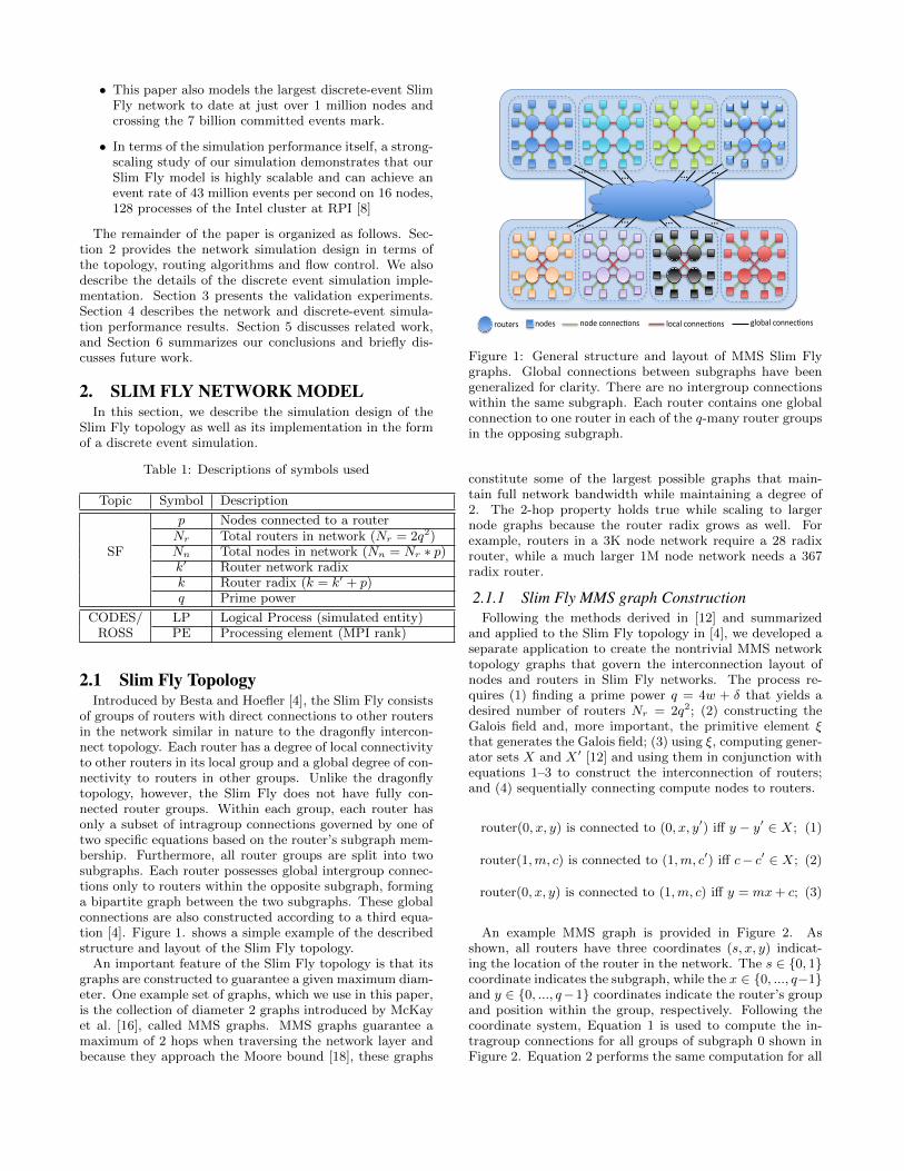
2.1.1 Slim Fly MMS graph ConstructionFollowing the methods derived in [12] and summarized

and applied to the Slim Fly topology in [4], we developed aseparate application to create the nontrivial MMS networktopology graphs that govern the interconnection layout ofnodes and routers in Slim Fly networks. The process re-quires (1) finding a prime power q = 4w + δ that yields adesired number of routers Nr = 2q2; (2) constructing theGalois field and, more important, the primitive element ξthat generates the Galois field; (3) using ξ, computing gener-ator sets X and X ′ [12] and using them in conjunction withequations 1–3 to construct the interconnection of routers;and (4) sequentially connecting compute nodes to routers.

router(0, x, y) is connected to (0, x, y′) iff y − y′ ∈ X; (1)

router(1,m, c) is connected to (1,m, c′) iff c− c′ ∈ X; (2)

router(0, x, y) is connected to (1,m, c) iff y = mx+ c; (3)

An example MMS graph is provided in Figure 2. Asshown, all routers have three coordinates (s, x, y) indicat-ing the location of the router in the network. The s ∈ {0, 1}coordinate indicates the subgraph, while the x ∈ {0, ..., q−1}and y ∈ {0, ..., q−1} coordinates indicate the router’s groupand position within the group, respectively. Following thecoordinate system, Equation 1 is used to compute the in-tragroup connections for all groups of subgraph 0 shown inFigure 2. Equation 2 performs the same computation for all

groups in subgraph 1, shown in red. Equation 3 determinesthe connections between the two subgraphs, shown in blue.For simplicity, Equation 3 connections are displayed only forrouter(1, 0, 0).

0,0,0# # #

0,0,3# # #

0,0,1# # #0,0,2# # #

0,1,0# # #

0,1,3# # #

0,1,1# # #0,1,2# # #

0,2,0# # #

0,2,3# # #

0,2,1# # #0,2,2# # #

0,3,0# # #

0,3,3# # #

0,3,1# # #0,3,2# # #

0,0,4# # #

0,1,4# # #

0,2,4# # #

0,3,4# # #

0,4,0# # #

0,4,3# # #

0,4,1# # #0,4,2# ##

0,4,4# # #

Figure 2: Example MMS graph with q = 5 illustrating theconnection of routers within groups and between subgraphs.

2.2 Routing AlgorithmsOur Slim Fly model currently supports three routing al-

gorithms for studying network performance: minimal, non-minimal, and adaptive routing.

2.2.1 Minimal RoutingThe minimal, or direct, routing algorithm routes all net-

work packets from source to destination using a maximumof two hops between routers (property of MMS graphs guar-antees router graph diameter of two regardless of the size ofthe graph). If the source router and destination router aredirectly connected, then the minimal path consists of onlyone hop between routers. If the source compute node is con-nected to the same router as the destination compute node,then there are zero hops between routers. In the third case,an intermediate router must exist that shares a connectionto both source and destination router so the packet traversesa maximum of two hops.

2.2.2 Non-minimal RoutingNon-minimal routing for the Slim Fly topology follows the

traditional Valiant randomized routing algorithm [25]. Thisapproach selects a random intermediate router that is differ-ent from the source or destination router and routes mini-mally from source router to the randomly selected intermedi-ate router. The packet is then routed minimally again fromthe intermediate router to the destination router. The num-ber of hops traversed with valiant routing would be doublethat of minimal routing. In the optimal case when all threerouters are directly connected, the path will be two hops.On the other end of the spectrum each minimal path to andfrom the intermediate router can have two hops, bringingthe maximum number of possible hops to four.

2.2.3 Adaptive RoutingAdaptive routing mixes both minimal and non-minimal

approaches by adaptively selecting between the minimal pathand several valiant paths. To make direct comparisons forvalidating our model, we follow a slightly modified versionof the Universal Globally-Adaptive Load-balanced (UGAL)algorithm [26] shown in [14]. First, the minimal path andseveral non-minimal paths (nI) are generated and their cor-responding path lengths LM and Li

I , i ∈ 1, 2, ...nI are com-puted. Next, we compute the penalty c = Li

I/LM ∗ cSF ,where cSF is a constant chosen to balance the ratio. Next,

Figure 3: Worst-case traffic layout for the Slim Fly topology.

the final cost of each non-minimal route CiI = c ∗ qiI is com-

puted, where qiI is the occupancy of the first router’s outputport corresponding to the path of route i. The cost of theminimal path is simply the occupancy of the first router’sport along the path qM . Then, the route with the lowestcost is selected, and the packet is routed accordingly. Withthis method, each packet has a chance of getting routed withanywhere from one to four hops.

2.3 Traffic WorkloadsTo accurately simulate and analyze the network commu-

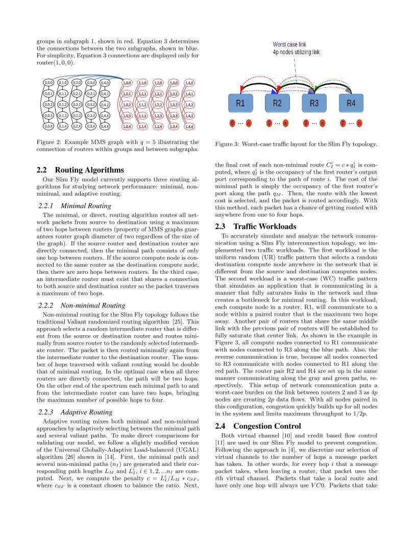
nication using a Slim Fly interconnection topology, we im-plemented two traffic workloads. The first workload is theuniform random (UR) traffic pattern that selects a randomdestination compute node anywhere in the network that isdifferent from the source and destination computes nodes.The second workload is a worst-case (WC) traffic patternthat simulates an application that is communicating in amanner that fully saturates links in the network and thuscreates a bottleneck for minimal routing. In this workload,each compute node in a router, R1, will communicate to anode within a paired router that is the maximum two hopsaway. Another pair of routers that share the same middlelink with the previous pair of routers will be established tofully saturate that center link. As shown in the example inFigure 3, all compute nodes connected to R1 communicatewith nodes connected to R3 along the blue path. Also, thereverse communication is true, because all nodes connectedto R3 communicate with nodes connected to R1 along thered path. The router pair R2 and R4 are set up in the samemanner communicating along the gray and green paths, re-spectively. This setup of network communication puts aworst-case burden on the link between routers 2 and 3 as 4pnodes are creating 2p data flows. With all nodes paired inthis configuration, congestion quickly builds up for all nodesin the system and limits maximum throughput to 1/2p.

2.4 Congestion ControlBoth virtual channel [10] and credit based flow control

[11] are used in our Slim Fly model to prevent congestion.Following the approach in [4], we discretize our selection ofvirtual channels to the number of hops a message packethas taken. In other words, for every hop i that a messagepacket takes, when leaving a router, that packet uses theith virtual channel. Packets that take a local route andhave only one hop will always use V C0. Packets that take

a global path (assuming minimal routing) will use V C0 forthe first hop and then V C1 for the second hop. Clearly, theoptimal number of VCs to use in minimal routing is two. Inthe case of non-minimal routing such as valiant and adaptiverouting, the number of virtual channels used is four, becausethe maximum possible number of hops in a packet’s route isfour.

In terms of the implementation, an output vc variable isadded to the compute node message state structure and ini-tialized to 0 when a message is created. Each time a routersends a message, it sends the message on the output vcvirtual channel and increments output vc so that the nextrouter on the path will use the next corresponding VC.

Each compute node and router also follows credit basedflow control by utilizing a buffer space to store packets need-ing to be injected into the network. When a credit is re-ceived, indicating the requested link is available for trans-mission, a packet in the corresponding link buffer is trans-mitted.

2.5 Discrete-Event SimulationCapturing performance measurements of extreme-scale net-

works having millions of nodes requires a simulation that canefficiently decompose the large problem domain. One suchapproach, used in this paper, is parallel discrete-event simu-lation (PDES). PDES decomposes the problem into distinctcomponents called logical processes (LPs), each with its ownself maintained state in the system. These LPs model thespecific computing components in the simulation such asrouters, nodes, and workload processes. LPs interact andcapture the system dynamics by passing timestamped eventmessages to one another. These LPs are further mapped tophysical MPI rank processing elements (PEs), which com-pute their corresponding LPs’ events in timestamped order.

We have implemented our Slim Fly model using ROSS [6],a discrete event simulator with support for both conserva-tive and optimistic parallel execution. Conservative execu-tion uses the YAWNS protocol [21] to keep all LPs fromcomputing events out of order. The optimistic event sched-uler allows each LP to keep its own local time and thereforecompute events out of order with respect to other LPs. Opti-mistic event scheduling is faster than conservative schedul-ing. However, this speedup comes at the cost of out-of-order event execution, which is handled by reverse compu-tation [7]. When a temporal anomaly occurs and an eventis processed out of timestamp order, all events must be in-crementally rolled back to restore the state of the LP to justbefore the incorrect event occurred.

The rollback process uses a reverse event handler to undothe events. The reverse handlers for the model must be pro-vided by the model programmers. The reverse event handleris a negation of the forward event handler performing inverseoperations on all state changing actions. For example, in theSlim Fly model using non-minimal routing, when a messagepacket arrives at its first router from a node, that router LPperforms forward operations in the router-receive forwardevent handler. The router LP (1) increments the numberof received packets, (2) sends a credit event to the sendingnode LP, (3) computes the next destination by sampling arandom number for the random intermediate destination,and (4) creates a new router-send event to relay the packetto the next hop router LP. The reverse event handler needsto undo these operations by (1) decrementing the received

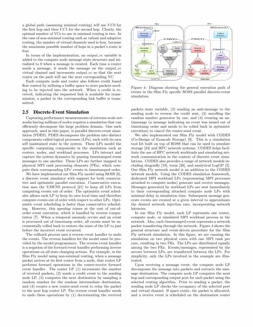
Figure 4: Diagram showing the general execution path ofevents in the Slim Fly specific ROSS parallel discrete-eventsimulation.

packets state variable, (2) sending an anti-message to thesending node to reverse the credit sent, (3) unrolling therandom number generator by one, and (4) creating an an-timessage (a message indicating an event was issued out oftimestamp order and needs to be rolled back in optimisticexecution) to cancel the router-send event.

We also implemented our Slim Fly model with CODES(Co-Design of Exascale Storage) [9]. This is a simulationtool kit built on top of ROSS that can be used to simulatestorage [24] and HPC network systems. CODES helps facil-itate the use of HPC network workloads and simulating net-work communication in the context of discrete event simu-lations. CODES also provides a range of network models in-cluding dragonfly [19], torus [20], and analytical LogGP [2].Our Slim Fly network model is an addition to the CODESnetwork models. Using the CODES simulation framework,dedicated MPI workload LPs (representing MPI processesattached to compute nodes) generate and receive messages.Messages generated by workload LPs are sent immediatelyto their corresponding attached compute node LPs withminimal delay in simulation time. Subsequent message gen-erate events are created at a given interval to approximatethe desired network injection rate, incorporating networklatencies.

In our Slim Fly model, each LP represents one router,compute node, or simulated MPI workload process in thenetwork. Also, each timestamped event represents a networkpacket transferring through the network. Figure 4 shows thegeneral structure and event-driven procedure for the SlimFly network simulation. In this figure, we are running thesimulation on two physical cores with one MPI rank percore, resulting in two PEs. The LPs are distributed equallyamong the two PEs. Events/messages, represented by thearrows between LPs, are transferred between the LPs. Forsimplicity, only the LPs involved in the example are illus-trated.

Upon receiving a message event, the compute node LPdecomposes the message into packets and extracts the mes-sage destination. The compute node LP computes the nexthop and corresponding output port for each packet using theselected routing algorithm. Prior to sending a packet, thesending node LP checks the occupancy of the selected portand virtual channel. If space exists, the packet is allocated,and a receive event is scheduled on the destination router

with a time delay. This time delay incorporates the band-width and latency of the corresponding network link. If thebuffer is full, the node LP follows credit-based flow controland must wait for a credit from the destination router toopen up a space on the corresponding link.

In order to accurately analyze the Slim Fly network, var-ious parameters and statistics are collected and stored inboth the LPs and the event messages. These statistics in-clude start and end times of packets on the network, averagehops traversed by the packets, and the virtual channels be-ing used.

Once a packet arrives at the router LP, a credit event issent back to the sending LP to free up space in the send-ing LP’s output buffer. The LP then extracts the desti-nation node ID. The router LP determines the next hopand corresponding output port, once again using the rout-ing algorithm specified. The router also follows the samecredit-based flow control scheme as the compute node LP.

After the packet reaches its destination node LP, the nodewaits for all packets belonging to that message to arrive be-fore issuing a message arrival event on the destination work-load LP. At this point, we can collect the statistics storedin the messages, for example, packet latency and number ofhops traversed.

3. SLIM FLY MODEL VALIDATIONIn this section, we present a comparison with published

Slim Fly network results by Kathareios et al. [14] to vali-date the implementation of our model. The specifics of theIBM-ETH-SF simulator are not provided, but the authorsdo mention that it is based on the Omnest simulator, whichalso employs parallel discrete-event simulation. This IBM-ETH collaborative work presents throughput results for aSlim Fly network with the configuration below. The con-figuration is of particular interest because it yields a totalnumber of compute nodes that is similar to the number ofnodes in the future Summit supercomputer [22].

• q = 13, p = 9, Nn = 3042, Nr = 338, k = 28.

Further network parameters include a 100 Gbps link band-width for all links with a latency of 50 ns. The routers utilizevirtual channels, a buffer space of 100 KB per port (equallydivided among the VCs), and a 100 ns traversal delay. Flowcontrol is done with the use of credits and messages are 256byte packets. Simulation time for the IBM-ETH-SF was200 µs with a 20 µs warmup. In our simulation, we in-clude the warmup time in the total execution and thereforerun the simulation for 220 µs. The results include mini-mal, non-minimal, and adaptive routing for uniform randomand worst-case traffic workloads. Our simulation results incomparison with the IBM-ETH-SF results are presented inFigures 5, 6, and 7. The metric comparison is throughputpercentage and is computed according to Equation 4. Bestaand Hoefler [4] approximate the upper bound for bisectionbandwidth for the Slim Fly topology to be 71% link band-

width per node when p = b k′

2c. Therefore, our simulated 100

Gbps link bandwidth translates to a maximum throughputof 71 Gbps per node. The observed throughput is gainedfrom our Slim Fly model by performing a sum reduction toget the total number of packets transferred by all computenodes, multiplying by the 256 byte packet size and dividingby the total number of compute nodes.

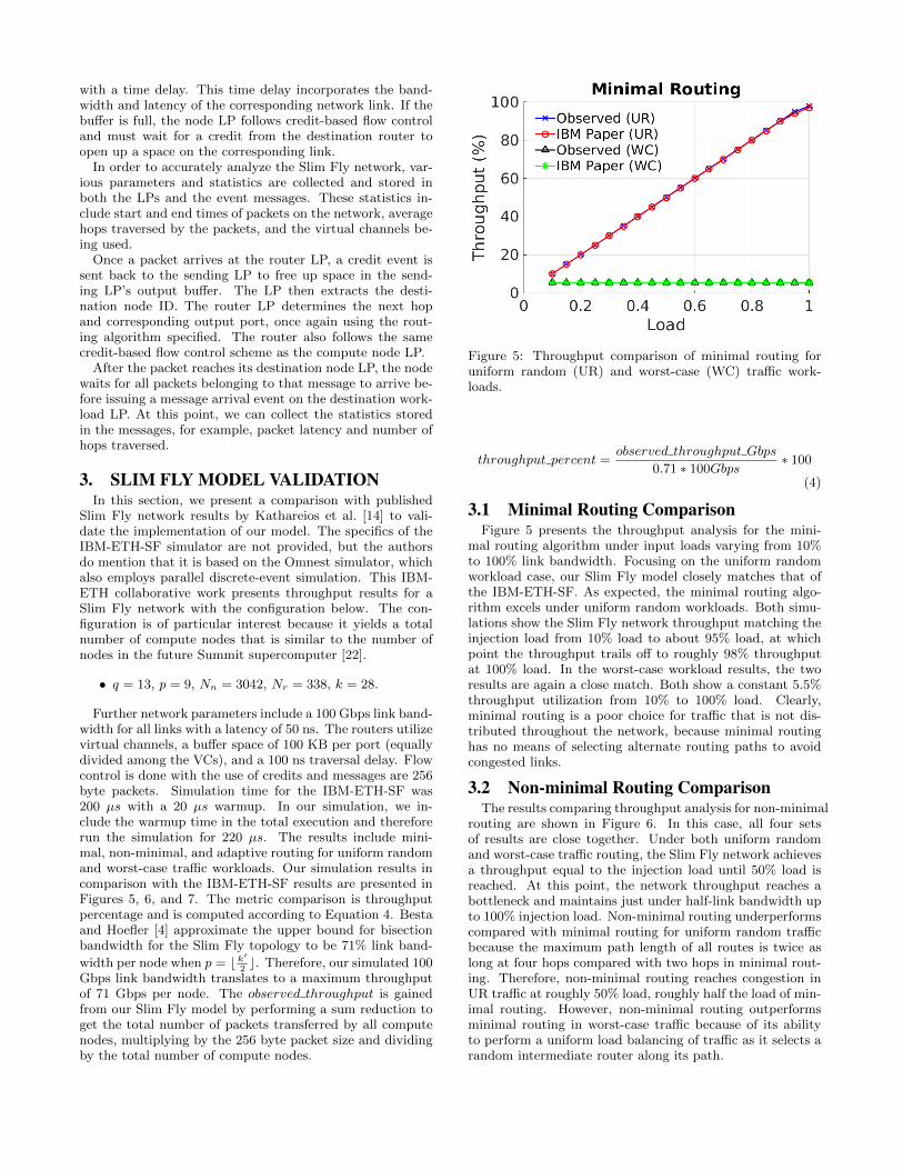
Figure 5: Throughput comparison of minimal routing foruniform random (UR) and worst-case (WC) traffic work-loads.

throughput percent =observed throughput Gbps

0.71 ∗ 100Gbps∗ 100

(4)

3.1 Minimal Routing ComparisonFigure 5 presents the throughput analysis for the mini-

mal routing algorithm under input loads varying from 10%to 100% link bandwidth. Focusing on the uniform randomworkload case, our Slim Fly model closely matches that ofthe IBM-ETH-SF. As expected, the minimal routing algo-rithm excels under uniform random workloads. Both simu-lations show the Slim Fly network throughput matching theinjection load from 10% load to about 95% load, at whichpoint the throughput trails off to roughly 98% throughputat 100% load. In the worst-case workload results, the tworesults are again a close match. Both show a constant 5.5%throughput utilization from 10% to 100% load. Clearly,minimal routing is a poor choice for traffic that is not dis-tributed throughout the network, because minimal routinghas no means of selecting alternate routing paths to avoidcongested links.

3.2 Non-minimal Routing ComparisonThe results comparing throughput analysis for non-minimal

routing are shown in Figure 6. In this case, all four setsof results are close together. Under both uniform randomand worst-case traffic routing, the Slim Fly network achievesa throughput equal to the injection load until 50% load isreached. At this point, the network throughput reaches abottleneck and maintains just under half-link bandwidth upto 100% injection load. Non-minimal routing underperformscompared with minimal routing for uniform random trafficbecause the maximum path length of all routes is twice aslong at four hops compared with two hops in minimal rout-ing. Therefore, non-minimal routing reaches congestion inUR traffic at roughly 50% load, roughly half the load of min-imal routing. However, non-minimal routing outperformsminimal routing in worst-case traffic because of its abilityto perform a uniform load balancing of traffic as it selects arandom intermediate router along its path.

Figure 6: Throughput comparison of non-minimal routingfor uniform random (UR) and worst-case (WC) traffic work-loads.

Figure 7: Throughput comparison of adaptive routing forUniform Random (UR) and worst-case (WC) traffic work-loads.

3.3 Adaptive Routing ComparisonThe throughput comparison results for the adaptive rout-

ing algorithm are shown in Figure 7. In all cases, we setthe number of indirect routes, ni = 3, and cSF = 1. Onceagain, the observed results for our Slim Fly model agree withthose of the IBM-ETH-SF simulator. In both uniform ran-dom and worst-case traffic workloads, the network through-put matches the injection load until 55% load, at which pointthe worst-case traffic results reach congestion and are limitedat 58%. The uniform random traffic results continue withoptimal throughput and reach nearly full system through-put at 100% load. Adaptive routing is able to match theperformance of minimal routing for uniform random traf-fic because it can continually select the minimal path forall packets. Adaptive routing outperforms both minimaland non-minimal routing for worst-case traffic because ofits ability to dynamically select between the minimal andnon-minimal routes.

3.4 Network VisualizationContinuing the analysis, we show visual representations of

router occupancy and message sends and receives for bothrouter LPs and compute node LPs during the above simula-tions. These visualizations provide insight into large, com-plex network simulations.

The router occupancy metric collects the number of pack-ets sitting in queue waiting for space to open up on the nec-essary router output port. Since we use VCs for congestioncontrol, the router occupancy metric can be further dividedinto virtual channels with 2 VCs per port per router used inthe case of minimal routing and 4 VCs per port per routerused in non-minimal routing. Since virtual channels helpalleviate congestion, their occupancy can provide insight tohelp identify the source of congestion in the network.

Figure 8 presents a number of graphs visualizing the occu-pancy of all virtual channels for all ports on all routers in thesimulation. All four Slim Fly test cases are from Figure 5,which run the 3K-node Slim Fly model using minimal rout-ing for uniform random traffic. In this case, there are 338routers with a network radix of 19 and 2 VCs per port. Theresult is a total of 6,422 ports, each with 2 virtual channels.Figures 8a–8d display the occupancy of VC0 with increasingload from 50% to 100%, and Figures 8e–8h display the samefor VC1.

The 3K-node Slim Fly model experiences little congestionuntil about 90% injection load, where VC0 sees a uniformdistribution of roughly 20% congestion in the network. At100% injection load, the network begins to reach the bufferspace limit as packets enter the network at an increased rate,further explaining why we see a slight dip in throughput per-formance for minimal routing under uniform random trafficin Figure 5. The VC0 buffer fills up first, indicating that thecompute nodes are injecting packets into the network fasterthan the routers can relay them.

In addition to buffer occupancy, the number of messagepackets sent and received by all routers and compute nodesis visualized over the simulation time. The results are col-lected during the same simulation in Figures 8d and 8h andare displayed in Figure 9. The first noticeable feature is thelarge spike in the beginning of the compute node sends (Fig-ure 9a). Occurring at the beginning of the simulation, thisspike is a result of the initial packet burst into the system,which is followed by a balancing out as the network reachesa steady state. The same phenomenon is reflected as a slowstart in router sends and receives plots in Figures 9c and 9d.These figures all resemble the uniform random traffic work-load being simulated, except for the initial startup phase.We can also note that the steady-state section of the routersends graph has more of a yellow hue than does the routerreceives plot, indicating that the routers consistently receivemessage packets but have slightly more variance in the rateat which they are able to send packets, which can contributeto the slight drop in network throughput observed at 100%load.

The added capability of visual analysis of these impor-tant network metrics not only helps detect network conges-tion but also helps identify the time, location, and effect ofcongestion on the entire network simulation.

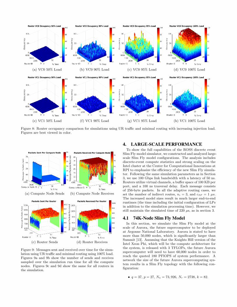
(a) VC0 50% Load (b) VC0 90% Load (c) VC0 95% Load (d) VC0 100% Load

(e) VC1 50% Load (f) VC1 90% Load (g) VC1 95% Load (h) VC1 100% Load

Figure 8: Router occupancy comparison for simulations using UR traffic and minimal routing with increasing injection load.Figures are best viewed in color.

(a) Compute Node Sends (b) Compute Node Receives

(c) Router Sends (d) Router Receives

Figure 9: Messages sent and received over time for the simu-lation using UR traffic and minimal routing using 100% load.Figures 9a and 9b show the number of sends and receivessampled over the simulation run time for all the computenodes. Figures 9c and 9d show the same for all routers inthe simulation.

4. LARGE-SCALE PERFORMANCETo show the full capabilities of the ROSS discrete event

Slim Fly model simulator, we constructed and analyzed large-scale Slim Fly model configurations. The analysis includesdiscrete-event compute statistics and strong scaling on theIntel cluster at the Center for Computational Innovations atRPI to emphasize the efficiency of the new Slim Fly simula-tor. Following the same simulation parameters as in Section3, we use 100 Gbps link bandwidth with a latency of 50 ns.Routers utilize virtual channels, a buffer space of 100 KB perport, and a 100 ns traversal delay. Each message consistsof 256-byte packets. In all the adaptive routing cases, weset the number of indirect routes, ni = 3, and cSF = 1 µs.The increased model sizes result in much larger end-to-endruntimes (the time including the initial configuration of LPsin addition to the simulation processing time). However, westill maintain the simulated time of 220 µs, as in section 3.

4.1 74K-Node Slim Fly ModelIn this section, we simulate the Slim Fly model at the

scale of Aurora, the future supercomputer to be deployedat Argonne National Laboratory. Aurora is stated to havemore than 50,000 nodes, which is significantly larger thanSummit [13]. Assuming that the Knights Hill version of theIntel Xeon Phi, which will be the compute architecture forthe system, is released with 3 TFLOPs, the future Aurorasupercomputer will need to have 60,000 nodes in order toreach the quoted 180 PFlOPS of system performance. Anetwork the size of the future Aurora supercomputing sys-tem results in a Slim Fly topology with the following con-figuration:

• q = 37, p = 27, Nn = 73, 926, Nr = 2738, k = 82.

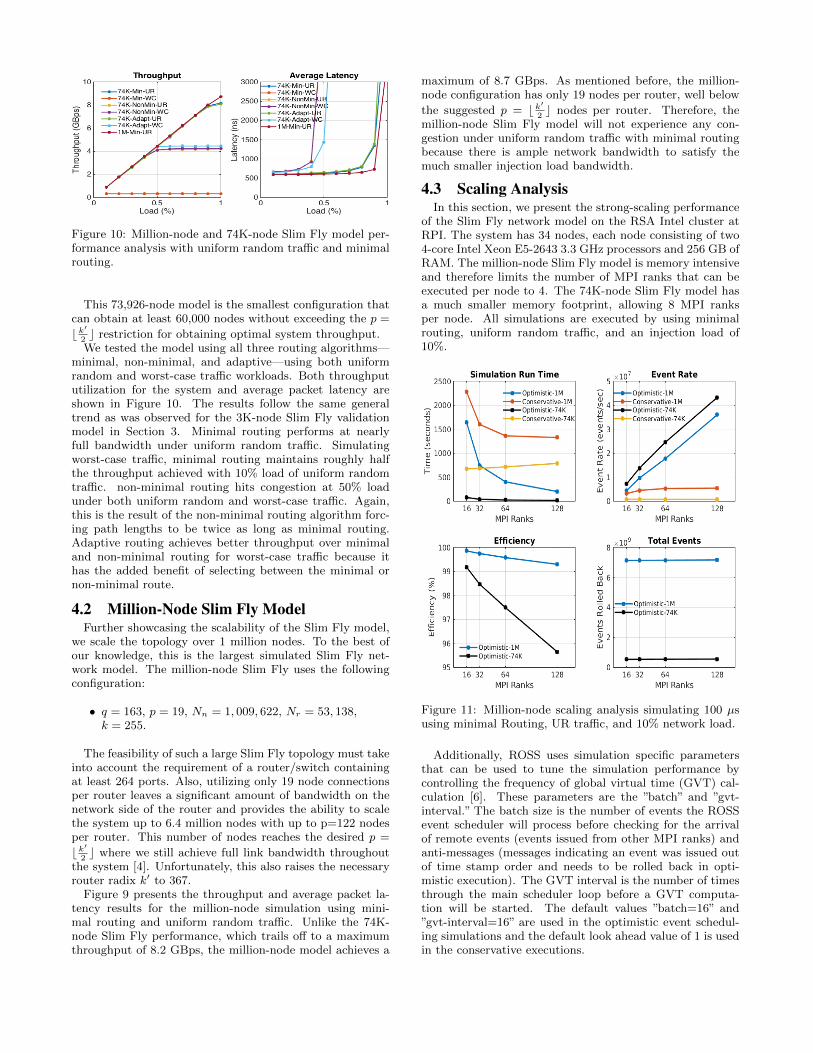
Figure 10: Million-node and 74K-node Slim Fly model per-formance analysis with uniform random traffic and minimalrouting.

This 73,926-node model is the smallest configuration thatcan obtain at least 60,000 nodes without exceeding the p =

b k′

2c restriction for obtaining optimal system throughput.

We tested the model using all three routing algorithms—minimal, non-minimal, and adaptive—using both uniformrandom and worst-case traffic workloads. Both throughpututilization for the system and average packet latency areshown in Figure 10. The results follow the same generaltrend as was observed for the 3K-node Slim Fly validationmodel in Section 3. Minimal routing performs at nearlyfull bandwidth under uniform random traffic. Simulatingworst-case traffic, minimal routing maintains roughly halfthe throughput achieved with 10% load of uniform randomtraffic. non-minimal routing hits congestion at 50% loadunder both uniform random and worst-case traffic. Again,this is the result of the non-minimal routing algorithm forc-ing path lengths to be twice as long as minimal routing.Adaptive routing achieves better throughput over minimaland non-minimal routing for worst-case traffic because ithas the added benefit of selecting between the minimal ornon-minimal route.

4.2 Million-Node Slim Fly ModelFurther showcasing the scalability of the Slim Fly model,

we scale the topology over 1 million nodes. To the best ofour knowledge, this is the largest simulated Slim Fly net-work model. The million-node Slim Fly uses the followingconfiguration:

• q = 163, p = 19, Nn = 1, 009, 622, Nr = 53, 138,k = 255.

The feasibility of such a large Slim Fly topology must takeinto account the requirement of a router/switch containingat least 264 ports. Also, utilizing only 19 node connectionsper router leaves a significant amount of bandwidth on thenetwork side of the router and provides the ability to scalethe system up to 6.4 million nodes with up to p=122 nodesper router. This number of nodes reaches the desired p =

b k′

2c where we still achieve full link bandwidth throughout

the system [4]. Unfortunately, this also raises the necessaryrouter radix k′ to 367.

Figure 9 presents the throughput and average packet la-tency results for the million-node simulation using mini-mal routing and uniform random traffic. Unlike the 74K-node Slim Fly performance, which trails off to a maximumthroughput of 8.2 GBps, the million-node model achieves a

maximum of 8.7 GBps. As mentioned before, the million-node configuration has only 19 nodes per router, well below

the suggested p = b k′

2c nodes per router. Therefore, the

million-node Slim Fly model will not experience any con-gestion under uniform random traffic with minimal routingbecause there is ample network bandwidth to satisfy themuch smaller injection load bandwidth.

4.3 Scaling AnalysisIn this section, we present the strong-scaling performance

of the Slim Fly network model on the RSA Intel cluster atRPI. The system has 34 nodes, each node consisting of two4-core Intel Xeon E5-2643 3.3 GHz processors and 256 GB ofRAM. The million-node Slim Fly model is memory intensiveand therefore limits the number of MPI ranks that can beexecuted per node to 4. The 74K-node Slim Fly model hasa much smaller memory footprint, allowing 8 MPI ranksper node. All simulations are executed by using minimalrouting, uniform random traffic, and an injection load of10%.

Figure 11: Million-node scaling analysis simulating 100 µsusing minimal Routing, UR traffic, and 10% network load.

Additionally, ROSS uses simulation specific parametersthat can be used to tune the simulation performance bycontrolling the frequency of global virtual time (GVT) cal-culation [6]. These parameters are the ”batch” and ”gvt-interval.” The batch size is the number of events the ROSSevent scheduler will process before checking for the arrivalof remote events (events issued from other MPI ranks) andanti-messages (messages indicating an event was issued outof time stamp order and needs to be rolled back in opti-mistic execution). The GVT interval is the number of timesthrough the main scheduler loop before a GVT computa-tion will be started. The default values ”batch=16” and”gvt-interval=16” are used in the optimistic event schedul-ing simulations and the default look ahead value of 1 is usedin the conservative executions.

The scaling performance results are evaluated according tosimulation run time (not including simulation configurationtime), event rate, event efficiency, and total number of pro-cessed events. These measurements provide insight into howwell the Slim Fly model performs as a ROSS discrete-eventsimulation. Event rate is a simple calculation of completedevents per second, and event efficiency describes how muchwork is being performed in the positive direction. Instead ofusing traditional state saving techniques, ROSS uses reverseevent handlers that undo untimely executed events. Thistechnique saves state but requires extra compute to unrollthe events. The simulation efficiency measures the amountof reverse computation using Equation 5 [3].

efficiency = 1− rolled back events

total events(5)

As shown in Fig. 7, utilizing the ROSS optimistic eventscheduler results in an ideal linear speedup of both the SlimFly million-node model and the 74K-mode model. The largestevent rate is achieved running the 74K-node Slim Fly modelon 128 MPI ranks, executing just over 43 million events persecond and processing 543 million events. Not far behind,the million-node model achieves a rate of 36 million eventsper second processing 7 billion events. Mapping the 7 bil-lion events to 128 MPI processes translates to each processstaying saturated with events and leads to an event effi-ciency above 99%. Running smaller Slim Fly configurationson as many processes leads to negative efficiency because ofless available work. At 128 MPI processes, the smaller 74K-node Slim Fly model has a 3% lower efficiency than does themillion-node model but manages to execute events at a 20%faster event rate. The smaller number of events per PE inthe 74K-node model translates to less overhead reorderingevents to maintain timestamp order.

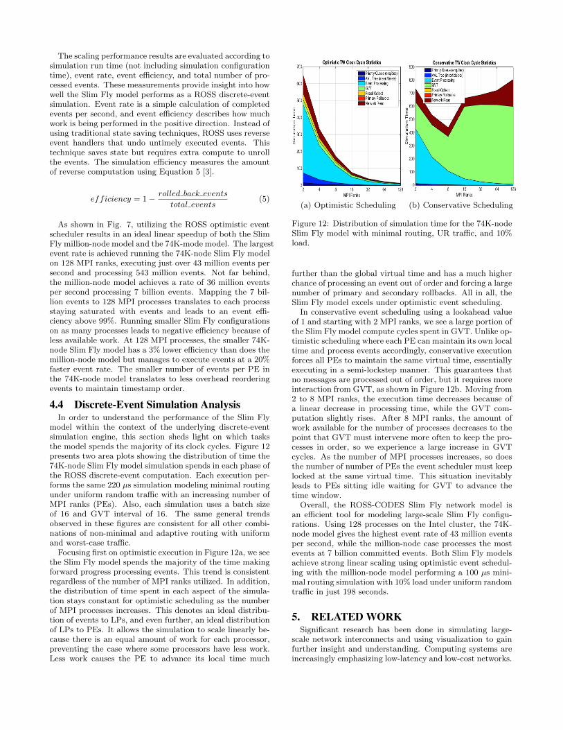
4.4 Discrete-Event Simulation AnalysisIn order to understand the performance of the Slim Fly

model within the context of the underlying discrete-eventsimulation engine, this section sheds light on which tasksthe model spends the majority of its clock cycles. Figure 12presents two area plots showing the distribution of time the74K-node Slim Fly model simulation spends in each phase ofthe ROSS discrete-event computation. Each execution per-forms the same 220 µs simulation modeling minimal routingunder uniform random traffic with an increasing number ofMPI ranks (PEs). Also, each simulation uses a batch sizeof 16 and GVT interval of 16. The same general trendsobserved in these figures are consistent for all other combi-nations of non-minimal and adaptive routing with uniformand worst-case traffic.

Focusing first on optimistic execution in Figure 12a, we seethe Slim Fly model spends the majority of the time makingforward progress processing events. This trend is consistentregardless of the number of MPI ranks utilized. In addition,the distribution of time spent in each aspect of the simula-tion stays constant for optimistic scheduling as the numberof MPI processes increases. This denotes an ideal distribu-tion of events to LPs, and even further, an ideal distributionof LPs to PEs. It allows the simulation to scale linearly be-cause there is an equal amount of work for each processor,preventing the case where some processors have less work.Less work causes the PE to advance its local time much

(a) Optimistic Scheduling (b) Conservative Scheduling

Figure 12: Distribution of simulation time for the 74K-nodeSlim Fly model with minimal routing, UR traffic, and 10%load.

further than the global virtual time and has a much higherchance of processing an event out of order and forcing a largenumber of primary and secondary rollbacks. All in all, theSlim Fly model excels under optimistic event scheduling.

In conservative event scheduling using a lookahead valueof 1 and starting with 2 MPI ranks, we see a large portion ofthe Slim Fly model compute cycles spent in GVT. Unlike op-timistic scheduling where each PE can maintain its own localtime and process events accordingly, conservative executionforces all PEs to maintain the same virtual time, essentiallyexecuting in a semi-lockstep manner. This guarantees thatno messages are processed out of order, but it requires moreinteraction from GVT, as shown in Figure 12b. Moving from2 to 8 MPI ranks, the execution time decreases because ofa linear decrease in processing time, while the GVT com-putation slightly rises. After 8 MPI ranks, the amount ofwork available for the number of processes decreases to thepoint that GVT must intervene more often to keep the pro-cesses in order, so we experience a large increase in GVTcycles. As the number of MPI processes increases, so doesthe number of number of PEs the event scheduler must keeplocked at the same virtual time. This situation inevitablyleads to PEs sitting idle waiting for GVT to advance thetime window.

Overall, the ROSS-CODES Slim Fly network model isan efficient tool for modeling large-scale Slim Fly configu-rations. Using 128 processes on the Intel cluster, the 74K-node model gives the highest event rate of 43 million eventsper second, while the million-node case processes the mostevents at 7 billion committed events. Both Slim Fly modelsachieve strong linear scaling using optimistic event schedul-ing with the million-node model performing a 100 µs mini-mal routing simulation with 10% load under uniform randomtraffic in just 198 seconds.

5. RELATED WORKSignificant research has been done in simulating large-

scale network interconnects and using visualization to gainfurther insight and understanding. Computing systems areincreasingly emphasizing low-latency and low-cost networks.

Liu et al. [15] demonstrate the effectiveness of applyingthe fat tree interconnect to large data centers. The work fo-cuses on the ability of fat tree networks to perform well underdata-center applications at large scale. Unlike our work thatcurrently focuses on HPC workloads, their work focuses onworkloads approximating the Hadoop MapReduce model.

Mubarak et al. [19] [20] demonstrate the performanceof both the torus and dragonfly network topologies usingsynthetic workloads at large scale. The simulations are alsoimplemented on top of the CODES and ROSS discrete-eventsimulation frameworks and run on IBM Blue Gene/P andBlue Gene/Q systems. Our work, in contrast, studies theperformance and scaling using an Intel cluster.

Bhatele [5] presents new methods that include visualiza-tion for identifying congestion in dragonfly networks anddeveloping new task mappings to allow for efficient use of re-sources. Still a relatively new topology, the Slim Fly modeldoes not have any real-world implementations. Therefore, itcan benefit from the same methods of simulation and visualanalysis to predict and limit congestion of possible futureSlim Fly systems, especially when executing multiple con-current tasks.

Acun et al. [1] present TraceR, a tool that replays theBigSim application traces on top of CODES network mod-els. TraceR provides the ability to test CODES networkmodels under real-world production application workloads.In contrast, our work simulates synthetic uniform randomand worst-case traffic workloads. Since the TraceR tool hasbeen interfaced with the CODES and ROSS frameworks, itcan be experimented with on the Slim Fly model.

6. CONCLUSIONS AND FUTURE WORKIn this paper, we presented a Slim Fly network simula-

tor developed using CODES and the parallel discrete-eventsimulation framework ROSS. Having implemented minimal,non-minimal, and adaptive routing algorithms specific to theSlim Fly model, we simulated the effectiveness of those rout-ing methods under uniform random and worst-case synthetictraffic workloads. The results of the Slim Fly model havebeen verified by using published results from Besta and Hoe-fler [4].

Furthermore, the Slim Fly network model has been shownto scale in network size from a 3,042 and 73,926 node sys-tems, inspired by the future Summit and Aurora supercom-puters, to a million-node system topology. Additionally, theSlim Fly model scales linearly in execution up to 128 MPIranks on the CCI RSA Intel cluster, achieving a peak eventrate of 43 million events per second with 543 million totalevents processed for the 74K-node Slim Fly model. Themillion-node model achieves 36 million events per secondprocessing 7 billion events.

Through visualization of network simulation metrics likebuffer utilization and message packet transfers, we get an in-sight into the behavior of large-scale HPC networks. Thesemethods provide the ability to view the entire network sim-ulation and identify the cause and effect of congestion.

Further scaling of the million-node model can also be per-formed to make full use of the simulated q = 163 MMSconfiguration. A Slim Fly configuration can maintain maxi-

mum link bandwidth up to p = b k′

2c total nodes per router.

The million-node model we have simulated has a networkradix of k′ = 255 and p = 19 nodes per router. However,this q = 163 MMS configuration can use up to p = 122 nodes

per router to get a 6.4 million-node model capable of main-taining full network throughput. Adding additional realisticworkloads that model real world applications is another fu-ture direction we plan to experiment with. We also planto explore other applications for future large-scale Slim Flynetwork interconnects by possibly simulating a large-scaleneuromorphic supercomputing system [17].

AcknowledgmentsThis work was supported by the Air Force Research Labora-tory (AFRL), under award number FA8750-15-2-0078. Thiswas also supported by the U.S. Department of Energy, Officeof Science, Advanced Scientific Computing Research, underContract DE-AC02-06CH11357.

7. REFERENCES[1] B. Acun, N. Jain, A. Bhatele, M. Mubarak,

C. Carothers, and L. Kale. Preliminary evaluation of aparallel trace replay tool for hpc network simulations.In S. Hunold, A. Costan, D. GimAl’nez, A. Iosup,L. Ricci, M. E. GAsmez Requena, V. Scarano, A. L.Varbanescu, S. L. Scott, S. Lankes, J. Weidendorfer,and M. Alexander, editors, Euro-Par 2015: ParallelProcessing Workshops, volume 9523 of Lecture Notesin Computer Science, pages 417–429. SpringerInternational Publishing, 2015.

[2] A. Alexandrov, M. F. Ionescu, K. E. Schauser, andC. Scheiman. Loggp: Incorporating long messages intothe logp model—one step closer towards arealistic model for parallel computation. InProceedings of the Seventh Annual ACM Symposiumon Parallel Algorithms and Architectures, SPAA ’95,pages 95–105, New York, NY, USA, 1995. ACM.

[3] P. D. Barnes, Jr., C. D. Carothers, D. R. Jefferson,and J. M. LaPre. Warp speed: Executing time warpon 1,966,080 cores. In Proceedings of the 1st ACMSIGSIM Conference on Principles of AdvancedDiscrete Simulation, SIGSIM PADS ’13, pages327–336, New York, NY, USA, 2013. ACM.

[4] M. Besta and T. Hoefler. Slim Fly: A Cost EffectiveLow-Diameter Network Topology. Nov. 2014.Proceedings of the International Conference on HighPerformance Computing, Networking, Storage andAnalysis (SC14).

[5] A. Bhatele. Task mapping on complex computernetwork topologies for improved performance.Technical report, LDRD Final Report, LawrenceLivermore National Laboratory, Oct. 2015.LLNL-TR-678732.

[6] C. D. Carothers, D. Bauer, and S. Pearce. Ross: Ahigh-performance, low memory, modular time warpsystem. In Proceedings of the Fourteenth Workshop onParallel and Distributed Simulation, PADS ’00, pages53–60, Washington, DC, USA, 2000. IEEE ComputerSociety.

[7] C. D. Carothers, K. S. Perumalla, and R. M.Fujimoto. Efficient optimistic parallel simulationsusing reverse computation. ACM Trans. Model.Comput. Simul., 9(3):224–253, July 1999.

[8] CCI. Rsa cluster, Nov. 2014.

[9] J. Cope, L. N., L. S., C. P., C. C. D., and R. R.Codes: Enabling co-design of multilayer exascale

storage architectures. In Proceedings of the Workshopon Emerging Supercomputing Technologies (WEST),Tuscon, AZ, USA, 2011.

[10] W. Dally. Virtual-channel flow control. Parallel andDistributed Systems, IEEE Transactions on,3(2):194–205, Mar 1992.

[11] W. Dally and B. Towles. Principles and Practices ofInterconnection Networks. Morgan KaufmannPublishers Inc., San Francisco, CA, USA, 2003.

[12] P. R. Hafner. Geometric realisation of the graphs ofmckay-miller-siran. Journal of Combinatorial Theory,Series B, 90(2):223–232, 2004.

[13] Intel. Ushering in a new era: Argonne nationallaboratory’s aurora system. Technical report, IntelCorporation, April 2015.

[14] G. Kathareios, C. Minkenberg, B. Prisacari,G. Rodriguez, and T. Hoefler. Cost-EffectiveDiameter-Two Topologies: Analysis and Evaluation.Nov. 2015. Accepted at IEEE/ACM InternationalConference on High Performance Computing,Networking, Storage and Analysis (SC15).

[15] N. Liu, A. Haider, X.-H. Sun, and D. Jin. Fattreesim:Modeling large-scale fat-tree networks for hpc systemsand data centers using parallel and discrete eventsimulation. In Proceedings of the 3rd ACM SIGSIMConference on Principles of Advanced DiscreteSimulation, SIGSIM PADS ’15, pages 199–210, NewYork, NY, USA, 2015. ACM.

[16] B. D. McKay, M. Miller, and J. Siran. A note on largegraphs of diameter two and given maximum degree.Journal of Combinatorial Theory, Series B, 74(1):110– 118, 1998.

[17] P. A. Merolla, J. V. Arthur, R. Alvarez-Icaza, A. S.Cassidy, J. Sawada, F. Akopyan, B. L. Jackson,N. Imam, C. Guo, Y. Nakamura, B. Brezzo, I. Vo,S. K. Esser, R. Appuswamy, B. Taba, A. Amir, M. D.Flickner, W. P. Risk, R. Manohar, and D. S. Modha.A million spiking-neuron integrated circuit with ascalable communication network and interface.Science, 345(6197):668–673, 2014.

[18] Miller, Mirka, Siran, and Jozef. Moore graphs andbeyond: a survey of the degree/diameter problem. TheElectronic Journal of Combinatorics [electronic only],DS14:61 p., electronic only–61 p., electronic only, 2005.

[19] M. Mubarak, C. D. Carothers, R. Ross, and P. Carns.Modeling a million-node dragonfly network usingmassively parallel discrete-event simulation. InProceedings of the 2012 SC Companion: HighPerformance Computing, Networking Storage andAnalysis, SCC ’12, pages 366–376, Washington, DC,USA, 2012. IEEE Computer Society.

[20] M. Mubarak, C. D. Carothers, R. B. Ross, andP. Carns. A case study in using massively parallelsimulation for extreme-scale torus network codesign.In Proceedings of the 2Nd ACM SIGSIM Conferenceon Principles of Advanced Discrete Simulation,SIGSIM PADS ’14, pages 27–38, New York, NY, USA,2014. ACM.

[21] D. M. Nicol. The cost of conservative synchronizationin parallel discrete event simulations. J. ACM,40(2):304–333, Apr. 1993.

[22] NVIDIA. Summit and sierra supercomputers: Aninside look at the u.s. department of energy’s newpre-exascale systems. Technical report, NVIDIA,November 2014.

[23] M. Papka, P. Messina, R. Coffey, and C. Drugan.Argonne Leadership Computing Facility 2014 annualreport. Mar 2015.

[24] S. Snyder, P. Carns, J. Jenkins, K. Harms, R. Ross,M. Mubarak, and C. Carothers. A case for epidemicfault detection and group membership in hpc storagesystems. In S. A. Jarvis, S. A. Wright, and S. D.Hammond, editors, High Performance ComputingSystems. Performance Modeling, Benchmarking, andSimulation, volume 8966 of Lecture Notes inComputer Science, pages 237–248. SpringerInternational Publishing, 2015.

[25] L. G. Valiant. A scheme for fast parallelcommunication. SIAM Journal on Computing,11(2):350–361, 1982.

[26] S.-J. Wang. Load-balancing in multistageinterconnection networks under multiple-pass routing.Journal of Parallel and Distributed Computing,36(2):189 – 194, 1996.