Modeled Differential Muon Flux Measurements for … Differential Muon Flux Measurements for...
1
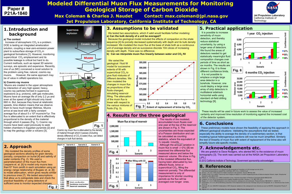
Modeled Differential Muon Flux Measurements for Monitoring Geological Storage of Carbon Dioxide Max Coleman & Charles J. Naudet Contact: [email protected] Jet Propulsion Laboratory, California Institute of Technology, CA Paper # P21A-1840 Jet Propulsion Laboratory California Institute of Technology Fig. 5 1.Introduction and background a) The context Increase of atmospheric CO 2 is a problem. DOE is testing an integrated amelioration solution, coupling a near-zero-emission power plant to subsurface storage of CO 2 in geological formations [1]. However, monitoring supercritical CO 2 emplacement and its possible leakage is critical but hard to do. Current methods, such as repeat 3D seismic surveys, are episodic and expensive. Recently, one of us (MC) conceived a novel solution to the problem using free, natural, cosmic-ray muons. However, the same approach may be of value in oilfield operations too. b) Cosmic-ray muons Muons are created in the upper atmosphere by interaction of very high speed, heavy, cosmic-ray particles formed in supernova explosions (e.g. protons), with gas molecules. Muons have an average life of only 2.2 !s and even at the speed of light should only travel 660 m. But, because they travel at relativistic speeds, time dilation means that we observe them to have much longer lifetimes. Muons arrive at sea level with a fairly constant average flux of about 5 x 10 9 muons/m 2 /yr. The flux is attenuated to an extent that is effectively proportional to the density of the material through which it passes (Fig. 1). Cosmic ray muons have been used previously to seek hidden chambers in Egyptian pyramids [2] and to map the geology under a volcano [3]. Cosmic ray muon flux is attenuated by the density of material through which it passes (including density difference of CO 2 & water) thus, can detect changes in bulk fluid density Fig. 1 2. Approach We modeled the density profiles of some geological sections allowing for grain density, porosity, compaction on burial [4] and salinity of water contents (Fig. 2). We used a parameterization of the muon flux from Lesparre et. al. [5] to model only muons less than10° from zenith in each simulation using an energy–range relationship of Bugaev et. al. [6] to model attenuation, which gives results similar to previous ones [7]. We tested assumptions that allow us to extrapolate data and check the practical feasibility of using detectors of sufficient area to monitor expected changes. Fig. 2 6. Conclusions These preliminary models have shown the feasibility of applying this approach in different geological situations .Validating the assumptions that we tested, especially the ability to average the density of a sedimentary section, is that modeling typical heterogeneous sections will now be much simplified. Similarly the test of linearity of muon flux with extent of replacement of the brine also will simplify future site-specific models. 5. Practical application 0 2,000 4,000 6,000 8,000 1 2 3 Detector area Scenario 1 year CO 2 injection 67% 95% 99% 0 5,000 10,000 15,000 20,000 25,000 30,000 1 2 3 Detector area Scenario 6 months CO 2 injection 67% 95% 99% Confidence limit Confidence limit Fig. 6 It is possible to increase sensitivity of muon detection, and thereby reduce statistical uncertainty, by using a larger area of detectors. We found the areas of detectors needed to get statistically meaningful fluid composition changes over periods of time as short as six months. The results are shown in Fig. 6 to three different confidence limits. It is not possible to emplace a single large area detector in a borehole. However, one could deploy a large area array of strip detectors in multilateral sidetrack horizontal wells using standard oil-field drilling technology [9]. These results will be used in future work to assess the value of increased certainty and improved time resolution of monitoring against the increased cost of the detector system. 7. Acknowledgements etc. We are grateful to Dave Rodgers, who alerted MC to the existence of muon tomography [3]. The work was carried out at the NASA Jet Propulsion Laboratory (JPL). © 2012 California Institute of Technology. Government sponsorship acknowledged. 8. References [1] FutureGen Industrial Alliance, Inc. Request for site proposals for FutureGen 2.0 CO2 storage hub site (2010). http://www.futuregenalliance.org/pdf/FGA_%20FINAL_RFP_FG_2_10252010.pdf [2] Alvarez, L.W. et al. (1970) Search for hidden chambers in the pyramids. Science 167 832–839. [3] Tanaka, H.K.M. et al. (2009) Cosmic-ray muon imaging of magma in a conduit: degassing process of Satsuma-Iwojima Volcano, Japan. Geophysical Research Letters 36 L01304. [4] Baldwin, B. and Butler, C.O. (1985) Compaction curves. American Association of Petroleum Geologists Bulletin 69 622-626. [5] Lesparre, N. et al. (2010) Geophysical muon imaging: feasibility and limits. Geophys. J. Int. 183 1348–1361. [6] Bugaev, E. V. et al. (1998) Atmospheric muon flux at sea level, underground, and underwater. Physical Review D 58 054001-1 - 054001-23. [7] Kudryavtsev, V.A. et al. (2012) Monitoring subsurface CO2 emplacement and security of storage using muon tomography. Int. Jl. Greenhouse Gas Control 11 21–24. [8] Ambrosio, M. et al. (MACRO Collaboration) (1997) Seasonal variations in the underground muon intensity as seen by MACRO: Astroparticle Physics 7 109-124. [9] Afghoul, A.C. et al. (2004) Coiled tubing: the next generation. Oilfield Review (Spring) 38–57. 3. Assumptions to be validated We tested two assumptions, which if valid would facilitate further modeling: a) Can the bulk density of a unit be averaged? Because the geological model included the effects of compaction on the shale sequence [4] its porosity decreased systematically with depth and its bulk density increased. We modeled the muon flux at the base of shale both as a continuous unit of average density and as successive discrete 10m slices of increasing density with depth. There was no difference. b) Can we nterpolate muon flux linearly between water and CO 2 fill We varied the geological / fluid fill model for successive extents of fill with supercritical CO 2 to give fluid mixtures of different densities. We then modeled the changes in muon flux as proportions of the fluids changed, simulating reservoir filling. The attenuation of the muon flux is linear with respect to the various mixtures of fluids (Fig. 3). 560,000 565,000 570,000 575,000 580,000 585,000 590,000 595,000 0.0 0.2 0.4 0.6 0.8 1.0 Muon flux Extent of replacement of brine by CO 2 Fig. 3 4. Results for the three geological scenarios ! #!!$!!! %$!!!$!!! %$#!!$!!! &$!!!$!!! % & ' ()*+,-./ 01/+ 213 ,4 4/5 /6 -*7*-8/.- Fig. 4 The results of the modeled, accumulated muon fluxes over one year at the top of the reservoir are shown in Fig. 4. The uncertainties are those expected of a Poisson distribution and can be calculated as counting statistics, where the equivalent of 1! equals "counts. Although the annual variation in muon flux is small (~2%) [8] we examined the differential flux measured above and below the reservoir volume. We show in Fig. 5 the modeled differential flux, having been attenuated by two different fluids, brine or supercritical CO 2 , filling the reservoir porosity. The differential measurement is only of importance for shorter counting periods as the flux will be averaged over longer ones. ! !#$ !#% !#& !#' !#( $ % & )*+, -./0 1.234506 -323-708- 9:3;.-80 <=3- >**8;? @85A BC% 2 Fig. 5
Transcript of Modeled Differential Muon Flux Measurements for … Differential Muon Flux Measurements for...
Modeled Differential Muon Flux Measurements for Monitoring Geological Storage of Carbon Dioxide
Max Coleman & Charles J. Naudet Contact: [email protected] Jet Propulsion Laboratory, California Institute of Technology, CA
Paper # P21A-1840 Jet Propulsion Laboratory
California Institute of Technology
Fig. 5
1.!Introduction and background
a) The context Increase of atmospheric CO2 is a problem. DOE is testing an integrated amelioration solution, coupling a near-zero-emission power plant to subsurface storage of CO2 in geological formations [1]. However, monitoring supercritical CO2 emplacement and its possible leakage is critical but hard to do. Current methods, such as repeat 3D seismic surveys, are episodic and expensive. Recently, one of us (MC) conceived a novel solution to the problem using free, natural, cosmic-ray muons. However, the same approach may be of value in oilfield operations too.
b) Cosmic-ray muons Muons are created in the upper atmosphere by interaction of very high speed, heavy, cosmic-ray particles formed in supernova explosions (e.g. protons), with gas molecules. Muons have an average life of only 2.2 !s and even at the speed of light should only travel 660 m. But, because they travel at relativistic speeds, time dilation means that we observe them to have much longer lifetimes. Muons arrive at sea level with a fairly constant average flux of about 5 x 10⁹ muons/m2/yr. The flux is attenuated to an extent that is effectively proportional to the density of the material through which it passes (Fig. 1). Cosmic ray muons have been used previously to seek hidden chambers in Egyptian pyramids [2] and to map the geology under a volcano [3]. Cosmic ray muon flux is attenuated by the density
of material through which it passes (including density difference of CO2 & water) thus, can detect changes in bulk fluid density
Fig. 1
2. Approach We modeled the density profiles of some geological sections allowing for grain density, porosity, compaction on burial [4] and salinity of water contents (Fig. 2). We used a parameterization of the muon flux from Lesparre et. al. [5] to model only muons less than10° from zenith in each simulation using an energy–range relationship of Bugaev et. al. [6] to model attenuation, which gives results similar to previous ones [7]. We tested assumptions that allow us to extrapolate data and check the practical feasibility of using detectors of sufficient area to monitor expected changes.
Fig. 2
6. Conclusions These preliminary models have shown the feasibility of applying this approach in different geological situations .Validating the assumptions that we tested, especially the ability to average the density of a sedimentary section, is that modeling typical heterogeneous sections will now be much simplified. Similarly the test of linearity of muon flux with extent of replacement of the brine also will simplify future site-specific models.
5. Practical application
0
2,000
4,000
6,000
8,000
1 2 3
Det
ecto
r ar
ea
Scenario
1 year CO2 injection
67%
95%
99%
0 5,000
10,000 15,000 20,000 25,000 30,000
1 2 3
Det
ecto
r ar
ea
Scenario
6 months CO2 injection
67%
95%
99%
Con
fiden
ce li
mit
Con
fiden
ce li
mit
Fig. 6
It is possible to increase sensitivity of muon detection, and thereby reduce statistical uncertainty, by using a larger area of detectors. We found the areas of detectors needed to get statistically meaningful fluid composition changes over periods of time as short as six months. The results are shown in Fig. 6 to three different confidence limits. It is not possible to emplace a single large area detector in a borehole. However, one could deploy a large area array of strip detectors in multilateral sidetrack horizontal wells using standard oil-field drilling technology [9].
These results will be used in future work to assess the value of increased certainty and improved time resolution of monitoring against the increased cost of the detector system.
7. Acknowledgements etc. We are grateful to Dave Rodgers, who alerted MC to the existence of muon tomography [3]. The work was carried out at the NASA Jet Propulsion Laboratory (JPL). © 2012 California Institute of Technology. Government sponsorship acknowledged.
8. References [1] FutureGen Industrial Alliance, Inc. Request for site proposals for FutureGen 2.0 CO2 storage hub site (2010).
http://www.futuregenalliance.org/pdf/FGA_%20FINAL_RFP_FG_2_10252010.pdf [2] Alvarez, L.W. et al. (1970) Search for hidden chambers in the pyramids. Science 167 832–839. [3] Tanaka, H.K.M. et al. (2009) Cosmic-ray muon imaging of magma in a conduit: degassing process of Satsuma-Iwojima Volcano, Japan. Geophysical
Research Letters 36 L01304. [4] Baldwin, B. and Butler, C.O. (1985) Compaction curves. American Association of Petroleum Geologists Bulletin 69 622-626. [5] Lesparre, N. et al. (2010) Geophysical muon imaging: feasibility and limits. Geophys. J. Int. 183 1348–1361. [6] Bugaev, E. V. et al. (1998) Atmospheric muon flux at sea level, underground, and underwater. Physical Review D 58 054001-1 - 054001-23. [7] Kudryavtsev, V.A. et al. (2012) Monitoring subsurface CO2 emplacement and security of storage using muon tomography. Int. Jl. Greenhouse Gas Control
11 21–24. [8] Ambrosio, M. et al. (MACRO Collaboration) (1997) Seasonal variations in the underground muon intensity as seen by MACRO: Astroparticle Physics 7
109-124. [9] Afghoul, A.C. et al. (2004) Coiled tubing: the next generation. Oilfield Review (Spring) 38–57.
3. Assumptions to be validated We tested two assumptions, which if valid would facilitate further modeling: a)! Can the bulk density of a unit be averaged? Because the geological model included the effects of compaction on the shale sequence [4] its porosity decreased systematically with depth and its bulk density increased. We modeled the muon flux at the base of shale both as a continuous unit of average density and as successive discrete 10m slices of increasing density with depth. There was no difference. b)! Can we nterpolate muon flux linearly between water and CO2 fill
We varied the geological / fluid fill model for successive extents of fill with supercritical CO2 to give fluid mixtures of different densities. We then modeled the changes in muon flux as proportions of the fluids changed, simulating reservoir filling. The attenuation of the muon flux is linear with respect to the various mixtures of fluids (Fig. 3).
560,000
565,000
570,000
575,000
580,000
585,000
590,000
595,000
0.0 0.2 0.4 0.6 0.8 1.0
Muo
n flu
x
Extent of replacement of brine by CO2 Fig. 3
4. Results for the three geological scenarios
…
!"
#!!$!!!"
%$!!!$!!!"
%$#!!$!!!"
&$!!!$!!!"
%" &" '"()*+,-./"
01/+"213",4"4/5"/6"-*7*-8/.-"
Fig. 4
The results of the modeled, accumulated muon fluxes over one year at the top of the reservoir are shown in Fig. 4. The uncertainties are those expected of a Poisson distribution and can be calculated as counting statistics, where the equivalent of 1! equals "counts. Although the annual variation in muon flux is small (~2%) [8] we examined the differential flux measured above and below the reservoir volume. We show in Fig. 5 the modeled differential flux, having been attenuated by two different fluids, brine or supercritical CO2, filling the reservoir porosity. The differential measurement is only of importance for shorter counting periods as the flux will be averaged over longer ones. !"
!#$"
!#%"
!#&"
!#'"
!#("
$" %" &"
)*+,"-./0"1.234506"
-323-708-"
9:3;.-80"
<=3-">**8;?"@85A"BC%" 2
Fig. 5