Model Simulation Studies of Model Simulation Studies of Hurricane Isabel in Chesapeake BayHurricane Isabel in Chesapeake Bay

Jian ShenJian ShenVirginia Institute of Marine SciencesVirginia Institute of Marine Sciences

College of William and MaryCollege of William and Mary

Isabel: Isabel: The 100-Year Storm !The 100-Year Storm !

Background of Storm Surge Modeling Background of Storm Surge Modeling • Numerical models have been successfully applied to

simulate and predict tide and storm surge in coastal seas – SLOSH (Sea, Lake, and Overland Surges for Hurricanes

– ADCIRC (Advanced Circulation Model)

• Impact of the storm surge at any particular location is sensitive to meteorological and topographic parameters

• Inundation is crucial for disaster planning • Prediction of flooding areas depends on model grid

resolution

New Challenges for Numerical ModelingNew Challenges for Numerical Modeling

• More high resolution terrain data are available– LIDAR (LIght Detection And Ranging)

• More real-time observation data are available– Surface elevation – Vertical velocity profile– Wave

• Real-time simulation vs. prediction– Rescue– Inundation

• How to integrate high resolution terrain and real-time observation data into models ?

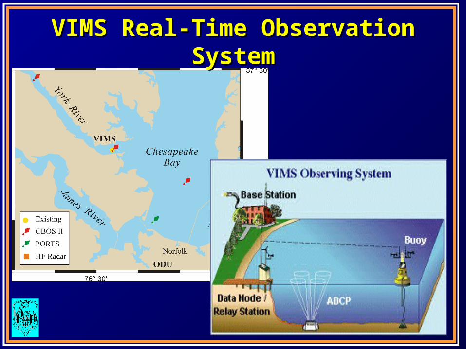
VIMS Real-Time Observation SystemVIMS Real-Time Observation System

Current Observation at Gloucester PointCurrent Observation at Gloucester Point

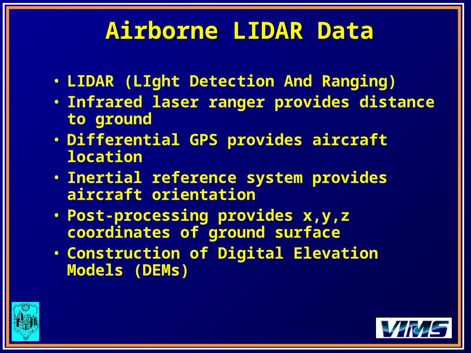
Airborne LIDAR DataAirborne LIDAR Data

• LIDAR (LIght Detection And Ranging)• Infrared laser ranger provides distance to

ground• Differential GPS provides aircraft location• Inertial reference system provides aircraft

orientation• Post-processing provides x,y,z coordinates of

ground surface• Construction of Digital Elevation Models

(DEMs)

DTMSDTMS

Legend

Elevation (NGVD 29, m)0 - 0.5

0.51 - 1

1.1 - 1.5

1.6 - 2

2.1 - 2.5

2.6 - 3

3.1 - 3.5

3.6 - 4

4.1 - 4.5

4.6 - 5

5.1 - 5.5

5.6 - 6

6.1 - 6.5

6.6 - 7

7.1 - 7.5

7.6 - 8

8.1 - 8.5

8.6 - 9

9.1 - 9.5

9.6 - 10

11 - 15

16 - 20

21 - 27

3 Sec (80-90 m) DTM Vertical Res. 1 m

10 DTM Vertical Res. 0.3 m

Elevation(feet)

Elevation(feet)

USGS 10m DEMUSGS 10m DEM LIDAR 10m DEMLIDAR 10m DEM

Example of LIDAR Data (Miami)Example of LIDAR Data (Miami)

Model Domain RepresentationModel Domain Representation• Small domain is inadequate for storm simulation• Coarse grid is inadequate to resolve irregular

shoreline and small topographic features in estuary• Structured grid is difficult to represent complex

bathymetric in estuary• Unstructured grid has advantage of storm surge

modeling– Use nested grids– Place fine grid in the areas of interest and coarse grid in

the remaining large areas

Model RequirementsModel Requirements

• Must resolve complex shoreline

• Must resolve land features– coastal ridge, dam, inlet, and river– small scale on the order of meters

• Must cover large modeling domain

• Must be computationally efficient

Example of Unstructured Grid (Miami)Example of Unstructured Grid (Miami)

Inlet

InletMiami River

Highway

Highway

0 2 km

Example of Nested Model GridsExample of Nested Model Grids

Unstructured 3D Model (UnTRIM)Unstructured 3D Model (UnTRIM)

• “UnTRIM” incorporates an Unstructured grid into TRIM model (Tidal, Residual, Intertidal Mudflat), originally developed by Vincenzo Casulli

• It simulates three-dimensional hydrodynamic and transport processes

• It uses an orthogonal unstructured grid• It conserves mass locally as well as globally • It uses Eulerian-Langangian transport scheme • It employs semi-implicit finite difference and finite

volume method- very efficient computationally• It is capable of simulating wet-dry processes

Grid StructureGrid Structure

• Use polygons to represent a prototype estuary (3-, 4-, 5-sides)

• Better fitting complicated geometry in estuarine and coastal environment

• Using orthogonal grid simplifies the numerical algorithm

Model Simulation StudiesModel Simulation Studies• Study the accuracy of model prediction of Isabel forced by

a stationary, circular wind model• Compare model prediction with and without simulating

inundation• Study influence of open boundary condition specification

on surge simulation– still boundary condition vs. inverse pressure adjust boundary

condition

• Study influence of model domain size on surge prediction• Study influence of wind field on model prediction• Study influence of hurricane on transport•

Model GridsModel Grids

Surface elements =121,338

Surface elements =239,541

Grid layouts at York and James RiversGrid layouts at York and James Rivers

Gloucester Pt.

0 2 km

0 2 km

Model CalibrationModel Calibration

• Calibrate model for tide

forced by 9 tidal constituents M2, S2, K1, O1, Q1, K2, N2, M4, and M6

• Model was run for 3 months and the results of the last 29 days were used for computing tidal harmonics

• Time step = 5 min.•

Tidal Simulation (MTidal Simulation (M22 tide) tide)

Tidal Simulation (KTidal Simulation (K11))

Observation StationsObservation Stations

Tidal Constituents Comparison Tidal Constituents Comparison (Amplitude)(Amplitude)

Amplitude is in mObservations are based on 1992 data

ModeledObs. ModeledObs. ModeledObs. ModeledObs. ModeledObs. ModeledObs.Stations

Bay Bridge 0.38 0.37 0.06 0.07 0.09 0.09 0.07 0.06 0.05 0.05 0.01 0.02Kiptopeke 0.38 0.37 0.06 0.07 0.08 0.09 0.07 0.06 0.05 0.05 0.01 0.02Sewells Pt. 0.35 0.35 0.06 0.06 0.08 0.08 0.06 0.06 0.05 0.04 0.01 0.02

Gloucester Pt. 0.34 0.33 0.05 0.06 0.07 0.08 0.05 0.05 0.04 0.04 0.01 0.02W indmill Point 0.17 0.16 0.03 0.03 0.04 0.04 0.04 0.03 0.02 0.02 0.01 0.01Lewisetta 0.18 0.17 0.04 0.03 0.04 0.04 0.03 0.02 0.02 0.02 0.02 0.01Solomons Isaland 0.17 0.16 0.03 0.02 0.03 0.04 0.04 0.03 0.03 0.02 0.02 0.01Cambridge 0.24 0.22 0.04 0.03 0.05 0.05 0.06 0.05 0.05 0.04 0.03 0.01Annapolis 0.12 0.13 0.02 0.02 0.03 0.03 0.06 0.06 0.05 0.04 0.01 0.01Baltimore 0.16 0.14 0.03 0.02 0.04 0.03 0.07 0.07 0.06 0.05 0.02 0.01Tolchester Beach 0.18 0.16 0.04 0.02 0.04 0.04 0.08 0.07 0.06 0.05 0.02 0.01

O1 K2M2 S2 N2 K1

Tidal Constituents Comparison (phase)Tidal Constituents Comparison (phase)

ModeledObs. ModeledObs. ModeledObs. ModeledObs. ModeledObs. ModeledObs.

Bay Bridge 99.5 99.5 75.1 75.1 39.4 39.4 199.3 199.3 268.3 268.3 224.7 224.7Kiptopeke 112.0 110.4 79.6 85.6 51.1 49.6 206.4 207.0 275.0 273.7 193.4 235.4Sewells Pt. 122.7 125.4 93.1 101.1 62.8 66.2 211.5 213.4 279.4 281.6 194.6 252.4Gloucester Pt. 130.6 131.9 101.8 105.6 71.3 72.8 215.4 211.3 283.0 281.4 163.3 259.3W indmill Point 181.9 196.4 152.8 166.9 119.1 130.9 241.7 242.9 312.7 313.5 298.9 15.6Lewisetta 254.0 253.9 203.8 231.0 185.6 189.0 289.0 288.3 360.7 355.4 324.8 18.5Solomons Isaland 270.9 276.5 211.9 254.3 202.7 210.2 319.0 329.1 24.4 27.4 325.1 43.8Cambridge 320.7 336.3 257.5 311.1 255.9 271.6 341.3 355.3 40.4 46.8 352.8 105.9Annapolis 7.1 8.8 319.6 348.0 300.8 305.9 0.9 10.1 56.3 65.2 58.9 133.0Baltimore 56.1 53.9 4.9 37.4 345.4 348.3 14.1 20.8 67.6 75.1 120.0 173.9Tolchester Beach 59.8 64.3 3.4 36.9 348.0 356.6 12.4 18.3 65.8 72.3 120.0 184.2

M2 S2Station N2 K1 O1 K2

Phase is in degree

Wind Model (Wind Model (Myers and Malkin, 1961) Myers and Malkin, 1961)

dr

dVV

Vk

dr

p

ps

a

sin

1 2

222

sincoscos1

Vkdr

dV

r

VfV

dr

p

p na

r = the distance from the storm centerp(r) = pressure, pa = central pressure, = the inflow angle across circular isobar toward the storm centerV is the wind speed, f = Coriolis parameter, ks and kn are friction coefficients.

Example of Wind FieldExample of Wind Field

-79 -78 -77 -76 -75 -74

34

35

36

37

38

39

40

5

10

10

15

15

20

20

20

25

2530

35

Isabel Simulation ResultsIsabel Simulation ResultsWith and Without Simulating inundationWith and Without Simulating inundation

Comparison of Model ResultsComparison of Model ResultsWith and Without Simulating InundationWith and Without Simulating Inundation

G loucester Point (with flooding)

-0.5

0

0.5

1

1.5

2

2.5

0 4 8 12 16 20 24 28 32 36 40 44 48 52 56 60 64 68 72

Hour (from 9/17/2003 0:00)

Ele

vati

on

(m

)

M odeledPredicted (HAM )O bserved

Sewells Point (without flooding)

-0.5

0

0.5

1

1.5

2

0 4 8 12 16 20 24 28 32 36 40 44 48 52 56 60 64 68 72

Hour (from 9/17/2003 0:00)

Ele

vati

on

(m

)

M odeledPrediced (HAM )O bserved

Sewells Point (with flooding)

-0.5

0

0.5

1

1.5

2

0 4 8 12 16 20 24 28 32 36 40 44 48 52 56 60 64 68 72

Hour (from 9/17/2003 0:00)

Ele

vati

on

(m

)

Modeled

Sweells Hall (HAM)

Observed

Gloucester Point (without flooding)

-0.5

0

0.5

1

1.5

2

2.5

0 4 8 12 16 20 24 28 32 36 40 44 48 52 56 60 64 68 72

Hour (from 9/17/2003 0:00)

Ele

vatio

n (m

)

ModeledPredicted (HAM)Observed

Comparison of Model ResultsComparison of Model ResultsWith and Without Simulating InundationWith and Without Simulating Inundation

Baltimore (with flood)

-0.5

0

0.5

1

1.5

2

2.5

0 4 8 12 16 20 24 28 32 36 40 44 48 52 56 60 64 68 72

Hour (from 9/17/2003 0:00)

Ele

vati

on

(m

)

M odeled Prediced (HAM )O bserved

Baltimore (without flood)

-0.5

0

0.5

1

1.5

2

2.5

0 4 8 12 16 20 24 28 32 36 40 44 48 52 56 60 64 68 72

Hour (from 9/17/2003 0:00)

Ele

vati

on

(m

)

M odeledPredicted (HAM )O bserved

Colonial Beach (with flood)

-0.5

0

0.5

1

1.5

2

0 4 8 12 16 20 24 28 32 36 40 44 48 52 56 60 64 68 72

Hour (from 9/17/2003 0:00)

Ele

vati

on

(m

)

M odeledPredicted (HAM )

Observed

Colonial Beach (without flood)

-0.5

0

0.5

1

1.5

2

2.5

0 4 8 12 16 20 24 28 32 36 40 44 48 52 56 60 64 68 72

Hour (from 9/17/2003 0:00)

Ele

vati

on

(m

)

M odeledPredicted (HAM )Observed

Test Influence of Open Boundary ConditionTest Influence of Open Boundary Condition• Apply inverse pressure adjustment at BC• Run large domain model (east coast) and apply

time series output from large domain model to force small domain model

Large Domain Model SimulationLarge Domain Model Simulation

Influence of Open Boundary ConditionInfluence of Open Boundary Condition

G loucester Point (with flooding)

-0.5

0

0.5

1

1.5

2

2.5

0 4 8 12 16 20 24 28 32 36 40 44 48 52 56 60 64 68 72

Hour (from 9/17/2003 0:00)

Ele

vati

on

(m

)

M odeledM odeled (IPABC)O bserved

Sewells Point (with flooding)

-0.5

0

0.5

1

1.5

2

0 4 8 12 16 20 24 28 32 36 40 44 48 52 56 60 64 68 72

Hour (from 9/17/2003 0:00)

Ele

vati

on

(m

)

Modeled

Modeled (IPABC)

Observed

Swelles Hall (with flooding)

-0.5

0

0.5

1

1.5

2

0 4 8 12 16 20 24 28 32 36 40 44 48 52 56 60 64 68 72

Hour (from 9/17/2003 0:00)

Ele

vati

on

(m

)

Time Series BC

IPABC

Observed

Gloucester Point (with flooding)

-0.5

0

0.5

1

1.5

2

2.5

0 4 8 12 16 20 24 28 32 36 40 44 48 52 56 60 64 68 72

Hour (from 9/17/2003 0:00)

Ele

vati

on

(m

)

Time series BCIPABCObserved

Inverse Pressure Adjustment

Nested Grids

Influence of Wind FieldInfluence of Wind Field

-79 -78 -77 -76 -75 -74

34

35

36

37

38

39

40

5

10

10

15

15

20

20

20

25

2530

35

Wind Field AnalysisWind Field Analysis

Comparison of Using Different Wind FieldsComparison of Using Different Wind Fields

Baltimore (with flood)

-0.5

0

0.5

1

1.5

2

2.5

0 4 8 12 16 20 24 28 32 36 40 44 48 52 56 60 64 68 72

Hour (from 9/17/2003 0:00)

Ele

vati

on (

m)

Modeled (Adj. wind parm.)

Modeled

Observed

Baltimore (with flood)

-0.5

0

0.5

1

1.5

2

2.5

0 4 8 12 16 20 24 28 32 36 40 44 48 52 56 60 64 68 72

Hour (from 9/17/2003 0:00)

Ele

vati

on

(m

)

M odeled Prediced (HAM )O bserved

Annapolis (with flooding)

-0.5

0

0.5

1

1.5

2

0 4 8 12 16 20 24 28 32 36 40 44 48 52 56 60 64 68 72

Hour (from 9/17/2003 0:00)

Ele

vati

on

(m

)

ModeledModeled (IPABC)Observed

Annapolis (with flood)

-0.5

0

0.5

1

1.5

2

0 4 8 12 16 20 24 28 32 36 40 44 48 52 56 60 64 68 72

Hour (from 9/17/2003 0:00)

Ele

vati

on (

m)

M odeled (Adj. w ind parm.)

M odeled

Observed

Current Simulation at Gloucester PointCurrent Simulation at Gloucester Point

Current Simulation at Gloucester Point (using local wind)

-1.0

-0.5

0.0

0.5

1.0

1.5

0 10 20 30 40 50 60 70 80 90 100

Hour (from 9/17/03 0:00)

Velo

city

(ms

-1)

obs. Suf obs. mid obs. Bottom Bottom mid surf

Current at Gloucester Point (Parametric wind model )

-1.0

-0.5

0.0

0.5

1.0

1.5

0 10 20 30 40 50 60 70

Hour (from 9/17/03 0:00 )

Vel

ocit

y (m

s-1

)

Obs. (surface) m/s Obs.(mid) m/s Obs. (bottom) m/sModeled(suface) Modeled(bottom) Modeled (Bottom)

Model Wind Field

Modified Wind Field

ConclusionsConclusions

• Unstructured model is very efficient in simulation tide and storm surge

• Open boundary condition specification influences the surge prediction

• Wind field is critical in the accurate simulation of storm surge

Thanks !Thanks !