Model Predictive Control Toolbox - Western...
128
For Use with MATLAB ® Getting Started Version 2 Model Predictive Control Toolbox Alberto Bemporad Manfred Morari N. Lawrence Ricker
Transcript of Model Predictive Control Toolbox - Western...
For Use with MATLAB®
Getting StartedVersion 2
Model Predictive ControlToolbox
Alberto BemporadManfred Morari
N. Lawrence Ricker
How to Contact The MathWorks:
www.mathworks.com Webcomp.soft-sys.matlab Newsgroup
[email protected] Technical [email protected] Product enhancement [email protected] Bug [email protected] Documentation error [email protected] Order status, license renewals, [email protected] Sales, pricing, and general information
508-647-7000 Phone
508-647-7001 Fax
The MathWorks, Inc. Mail3 Apple Hill DriveNatick, MA 01760-2098
For contact information about worldwide offices, see the MathWorks Web site.
Getting Started with the Model Predictive Control Toolbox © COPYRIGHT 2004-2005 by The MathWorks, Inc. The software described in this document is furnished under a license agreement. The software may be used or copied only under the terms of the license agreement. No part of this manual may be photocopied or repro-duced in any form without prior written consent from The MathWorks, Inc.
FEDERAL ACQUISITION: This provision applies to all acquisitions of the Program and Documentation by, for, or through the federal government of the United States. By accepting delivery of the Program or Documentation, the government hereby agrees that this software or documentation qualifies as commercial computer software or commercial computer software documentation as such terms are used or defined in FAR 12.212, DFARS Part 227.72, and DFARS 252.227-7014. Accordingly, the terms and conditions of this Agreement and only those rights specified in this Agreement, shall pertain to and govern the use, modification, reproduction, release, performance, display, and disclosure of the Program and Documentation by the federal government (or other entity acquiring for or through the federal government) and shall supersede any conflicting contractual terms or conditions. If this License fails to meet the government's needs or is inconsistent in any respect with federal procurement law, the government agrees to return the Program and Documentation, unused, to The MathWorks, Inc.
TrademarksMATLAB, Simulink, Stateflow, Handle Graphics, Real-Time Workshop, and xPC TargetBox are registered trademarks of The MathWorks, Inc. Other product or brand names are trademarks or registered trademarks of their respective holders.
PatentsThe MathWorks products are protected by one or more U.S. patents. Please see www.mathworks.com/patents for more information.

Revision History
October 2004 First printing New for Version 2.1 (Release 14SP1)March 2005 Online only Revised for Version 2.2 (Release 14SP2)September 2005 Online only Revised for Version 2.2.1 (Release 14SP3)

i
Contents
1Introduction
What Is the Model Predictive Control Toolbox? . . . . . . . . . . 1-2
Using the Documentation . . . . . . . . . . . . . . . . . . . . . . . . . . . . . . 1-4Related Products . . . . . . . . . . . . . . . . . . . . . . . . . . . . . . . . . . . . . 1-5
Bibliography . . . . . . . . . . . . . . . . . . . . . . . . . . . . . . . . . . . . . . . . . 1-6
2Building Models
Overview . . . . . . . . . . . . . . . . . . . . . . . . . . . . . . . . . . . . . . . . . . . . 2-2Plant Model . . . . . . . . . . . . . . . . . . . . . . . . . . . . . . . . . . . . . . . . . 2-2Plant Inputs and Outputs . . . . . . . . . . . . . . . . . . . . . . . . . . . . . . 2-3
Linear, Time Invariant (LTI) Models . . . . . . . . . . . . . . . . . . . . 2-4Transfer Function Format . . . . . . . . . . . . . . . . . . . . . . . . . . . . . 2-4Zero/Pole/Gain Format . . . . . . . . . . . . . . . . . . . . . . . . . . . . . . . . 2-5State-Space Format . . . . . . . . . . . . . . . . . . . . . . . . . . . . . . . . . . . 2-5LTI Object Properties . . . . . . . . . . . . . . . . . . . . . . . . . . . . . . . . . 2-7Multiinput Multioutput (MIMO) Plants . . . . . . . . . . . . . . . . . 2-11LTI Model Characteristics . . . . . . . . . . . . . . . . . . . . . . . . . . . . 2-13
System Identification Toolbox Models . . . . . . . . . . . . . . . . . 2-14System Identification Model Definition Example . . . . . . . . . . 2-14Converting a System Identification Toolbox Model to an LTI Object . . . . . . . . . . . . . . . . . . . . . . . . . . . . . . . . . . . . . . . . . 2-15Step-Response Models . . . . . . . . . . . . . . . . . . . . . . . . . . . . . . . . 2-17
Using Simulink to Develop LTI Models . . . . . . . . . . . . . . . . 2-19Linearization Using Simulink Control Design . . . . . . . . . . . . 2-19Linearization Using Simulink Functions . . . . . . . . . . . . . . . . . 2-24
ii Contents
Bibliography . . . . . . . . . . . . . . . . . . . . . . . . . . . . . . . . . . . . . . . . 2-26
3The Design Tool
Introduction . . . . . . . . . . . . . . . . . . . . . . . . . . . . . . . . . . . . . . . . . . 3-2Starting the Design Tool . . . . . . . . . . . . . . . . . . . . . . . . . . . . . . . 3-2Loading a Plant Model . . . . . . . . . . . . . . . . . . . . . . . . . . . . . . . . . 3-3Navigation Using the Tree View . . . . . . . . . . . . . . . . . . . . . . . . . 3-7
Linear Simulations . . . . . . . . . . . . . . . . . . . . . . . . . . . . . . . . . . . 3-12Defining Simulation Conditions . . . . . . . . . . . . . . . . . . . . . . . . 3-12Running a Simulation . . . . . . . . . . . . . . . . . . . . . . . . . . . . . . . . 3-14Open-Loop Simulations . . . . . . . . . . . . . . . . . . . . . . . . . . . . . . . 3-16
Changing Controller Settings . . . . . . . . . . . . . . . . . . . . . . . . . 3-19Model and Horizons . . . . . . . . . . . . . . . . . . . . . . . . . . . . . . . . . . 3-19Weight Tuning . . . . . . . . . . . . . . . . . . . . . . . . . . . . . . . . . . . . . . 3-21Blocking . . . . . . . . . . . . . . . . . . . . . . . . . . . . . . . . . . . . . . . . . . . 3-26Defining Manipulated Variable Constraints . . . . . . . . . . . . . . 3-29Disturbance Modeling and Estimation . . . . . . . . . . . . . . . . . . . 3-32
Defining Soft Output Constraints . . . . . . . . . . . . . . . . . . . . . . 3-40
Robustness Testing . . . . . . . . . . . . . . . . . . . . . . . . . . . . . . . . . . . 3-44Plant Model Perturbation . . . . . . . . . . . . . . . . . . . . . . . . . . . . . 3-44Simulation Tests . . . . . . . . . . . . . . . . . . . . . . . . . . . . . . . . . . . . 3-44
Plant Models with Delays . . . . . . . . . . . . . . . . . . . . . . . . . . . . . 3-47Importing the Plant Model . . . . . . . . . . . . . . . . . . . . . . . . . . . . 3-47Specifying Controller Horizons . . . . . . . . . . . . . . . . . . . . . . . . . 3-48
Nonsquare Plants . . . . . . . . . . . . . . . . . . . . . . . . . . . . . . . . . . . . 3-52More Outputs Than Manipulated Variables . . . . . . . . . . . . . . 3-52More Manipulated Variables Than Outputs . . . . . . . . . . . . . . 3-53
iii
Nonlinear Plants . . . . . . . . . . . . . . . . . . . . . . . . . . . . . . . . . . . . . 3-54The MPC Controller Block . . . . . . . . . . . . . . . . . . . . . . . . . . . . . 3-54Initiating the Controller Design . . . . . . . . . . . . . . . . . . . . . . . . 3-55Validating the Linearized Model . . . . . . . . . . . . . . . . . . . . . . . . 3-57Modifying the Linearized Model . . . . . . . . . . . . . . . . . . . . . . . . 3-59Linear Simulation Tests . . . . . . . . . . . . . . . . . . . . . . . . . . . . . . 3-60Nonlinear Simulation Tests . . . . . . . . . . . . . . . . . . . . . . . . . . . 3-62Modifying the Controller Using the Design Tool . . . . . . . . . . . 3-64Exiting the Design Tool . . . . . . . . . . . . . . . . . . . . . . . . . . . . . . . 3-64
Saving Your Work . . . . . . . . . . . . . . . . . . . . . . . . . . . . . . . . . . . . 3-65Exporting a Controller . . . . . . . . . . . . . . . . . . . . . . . . . . . . . . . . 3-65Saving a Project . . . . . . . . . . . . . . . . . . . . . . . . . . . . . . . . . . . . . 3-66
Loading Your Saved Work . . . . . . . . . . . . . . . . . . . . . . . . . . . . 3-67
4
Using Model Predictive Control ToolboxFunctions
Controller Definition . . . . . . . . . . . . . . . . . . . . . . . . . . . . . . . . . . 4-2Creating a Controller Object . . . . . . . . . . . . . . . . . . . . . . . . . . . . 4-2Viewing and Altering Controller Properties . . . . . . . . . . . . . . . . 4-3
Linear Simulations . . . . . . . . . . . . . . . . . . . . . . . . . . . . . . . . . . . . 4-6Using the sim Function . . . . . . . . . . . . . . . . . . . . . . . . . . . . . . . . 4-6Saving Calculated Results . . . . . . . . . . . . . . . . . . . . . . . . . . . . . . 4-6Simulation Options . . . . . . . . . . . . . . . . . . . . . . . . . . . . . . . . . . . 4-7
Simulations Involving Nonlinear Plants . . . . . . . . . . . . . . . . . 4-8A Nonlinear CSTR Application . . . . . . . . . . . . . . . . . . . . . . . . . . 4-8Example Code for Successive Linearization . . . . . . . . . . . . . . . . 4-9CSTR Results and Discussion . . . . . . . . . . . . . . . . . . . . . . . . . 4-10
Analysis Tools . . . . . . . . . . . . . . . . . . . . . . . . . . . . . . . . . . . . . . . 4-13Steady-State Gain Computation . . . . . . . . . . . . . . . . . . . . . . . . 4-13Controller Extraction . . . . . . . . . . . . . . . . . . . . . . . . . . . . . . . . . 4-13

iv Contents
Bibliography . . . . . . . . . . . . . . . . . . . . . . . . . . . . . . . . . . . . . . . . 4-15
Index

1
Introduction
What Is the Model Predictive Control Toolbox? (p. 1-2)
Compares the Model Predictive Control Toolbox to other common system control approaches
Using the Documentation (p. 1-4) Describes the available documentation
Bibliography (p. 1-6) Suggestions for further reading
1 Introduction
1-2
What Is the Model Predictive Control Toolbox?The Model Predictive Control Toolbox is a collection of software that helps you design, analyze, and implement an advanced industrial automation algorithm. Like other MATLAB® tools, it provides a convenient graphical user interface (GUI) as well as a flexible command syntax that supports customization.
A Model Predictive Control Toolbox controller automates a target system (the plant) by combining a prediction and a control strategy. An approximate plant model provides the prediction. The control strategy compares predicted plant signals to a set of objectives, then adjusts available actuators to achieve the objectives while respecting the plant’s constraints.
The controller’s constraint-tolerance differentiates it from other optimal control strategies (e.g., the Linear-Quadratic-Gaussian approach supported in the Control System Toolbox). The impetus for this is industrial experience suggesting that the drive for profitability often pushes the plant to one or more constraints. The Model Predictive Control Toolbox controller considers such factors explicitly, allowing it to allocate the available plant resources intelligently as the system evolves over time.
The Model Predictive Control Toolbox uses the same powerful linear dynamic modeling tools found in the Control System Toolbox and System Identification Toolbox. You can employ transfer functions, state-space matrices, or a combination. You can also include delays, which are a common feature of industrial plants.
If you don’t have a model but can perform experiments, the System Identification Toolbox provides methods to help you develop a data-based model for use in the Model Predictive Control Toolbox.
If you’d rather use the Simulink® graphical tools to model your plant, the Model Predictive Control Toolbox provides a special controller block for that environment. For example, you can linearize a nonlinear Simulink model, use the linearized model to build a Model Predictive Control Toolbox controller, and evaluate its ability to control the nonlinear model. Once that is working well, you can implement the control strategy in a real plant using Real Time Workshop®.
For a list of books on predictive control theory and practice, see “Bibliography” on page 1-6. In particular, Maciejowski [4] illustrates and extends Version 1.0

What Is the Model Predictive Control Toolbox?
1-3
of the Model Predictive Control Toolbox. (The command format used in [4] is obsolete in Model Predictive Control Toolbox Version 2.0, however.)

1 Introduction
1-4
Using the DocumentationIf you have limited experience with MATLAB or Model Predictive Control, read this guide first. It shows how to
• Define your plant using the Control System Toolbox modeling tools (LTI transfer function and state space models)
• Derive a linear plant model from a nonlinear Simulink representation
• Design Model Predictive Control for your plant using mpctool, the graphical user interface (GUI), or special commands
• Simulate Model Predictive Control performance using mpctool, Simulink, or commands
If you have experience with an earlier release of the Model Predictive Control Toolbox, we advise you to read this book to familiarize yourself with the many new features and the new command syntax (the earlier syntax is still available, but the underlying code is no longer supported).
If you need more details, see the online documentation. To access it type
helpdesk
at the MATLAB prompt. When the help dialog window appears, select Model Predictive Control Toolbox in the Contents pane. This displays a roadmap with links to the available documentation components. Briefly, these are
• “Getting Started.” The online version of this manual.
• “MPC Problem Setup.” Mathematical details of the Model Predictive Control Toolbox algorithm and user specifications required for controller design.
• “MPC Simulink Library.” Describes the Model Predictive Control Controller Block and its use within Simulink.
• “Case-Study Examples.” Example Toolbox applications.
• “The Design Tool.” Reference manual for mpctool, the GUI.
• “Functions.” Reference manual describing each Model Predictive Control Toolbox function (used for controller design and simulation in MATLAB commands and scripts).
• “Blocks.” Reference manual describing the Model Predictive Control Toolbox blocks (used for controller design and simulation in Simulink).
Using the Documentation
1-5
• “Object Reference.” Details of the controller object that represents a complete controller design.
• “Release Notes.” Summarizes major features of this release, known limitations, etc.
Related ProductsThe MathWorks provides other products that complement and enhance Model Predictive Control Toolbox functionality. See http://www.mathworks.com/products/mpc/ for more information.

1 Introduction
1-6
Bibliography[1] Allgower, F., and A. Zheng, Nonlinear Model Predictive Control, Springer-Verlag, 2000.
[2] Camacho, E. F., and C. Bordons, Model Predictive Control, Springer-Verlag, 1999.
[3] Kouvaritakis, B., and M. Cannon, Non-Linear Predictive Control: Theory & Practice, IEE Publishing, 2001.
[4] Maciejowski, J. M., Predictive Control with Constraints, Pearson Education POD, 2002.
[5] Prett, D., and C. Garcia, Fundamental Process Control, Butterworths, 1988.
[6] Rossiter, J. A., Model-Based Predictive Control: A Practical Approach, CRC Press, 2003.

2
Building Models
Overview (p. 2-2) Describes the model and input/output signal conventions used in the Model Predictive Control Toolbox
Linear, Time Invariant (LTI) Models (p. 2-4) Defines transfer function, zero-pole, and state-space models for use in the Model Predictive Control Toolbox
System Identification Toolbox Models (p. 2-14) Imports System Identification Toolbox (data-based) models for use in the Model Predictive Control Toolbox.
Using Simulink to Develop LTI Models (p. 2-19) Obtains a linear approximation of a nonlinear Simulink model.
2 Building Models
2-2
OverviewThis section covers the following topics:
• “Plant Model” on page 2-2
• “Plant Inputs and Outputs” on page 2-3
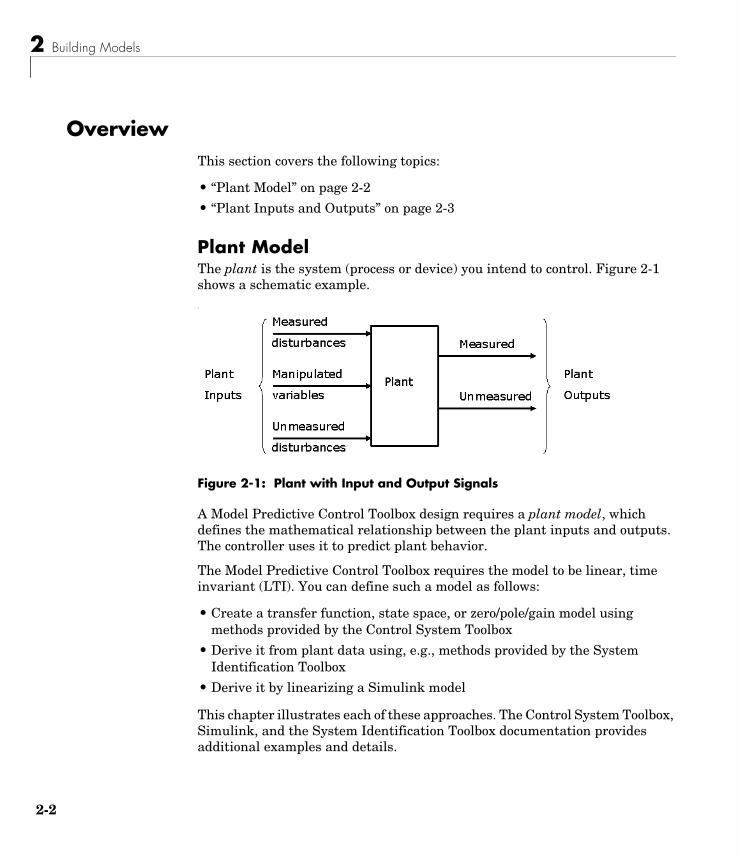
Plant ModelThe plant is the system (process or device) you intend to control. Figure 2-1 shows a schematic example..
Figure 2-1: Plant with Input and Output Signals
A Model Predictive Control Toolbox design requires a plant model, which defines the mathematical relationship between the plant inputs and outputs. The controller uses it to predict plant behavior.
The Model Predictive Control Toolbox requires the model to be linear, time invariant (LTI). You can define such a model as follows:
• Create a transfer function, state space, or zero/pole/gain model using methods provided by the Control System Toolbox
• Derive it from plant data using, e.g., methods provided by the System Identification Toolbox
• Derive it by linearizing a Simulink model
This chapter illustrates each of these approaches. The Control System Toolbox, Simulink, and the System Identification Toolbox documentation provides additional examples and details.

Overview
2-3
Plant Inputs and Outputs
InputsThe plant inputs are the independent variables affecting the plant. As shown in Figure 2-1, there are three types:
Measured disturbances. The controller can’t adjust them, but uses them for feedforward compensation.
Manipulated variables. The controller adjusts these in order to achieve its goals.
Unmeasured disturbances. These are independent inputs of which the controller has no direct knowledge, and for which it must compensate
OutputsThe plant outputs are the dependent variables (outcomes) you wish to control or monitor. As shown in Figure 2-1, there are two types:
Measured outputs. The controller uses these to estimate unmeasured quantities and as feedback on the success of its adjustments.
Unmeasured outputs. The controller estimates these based on available measurements and the plant model. The controller can also hold unmeasured outputs at setpoints or within constraint boundaries.
You must specify the input and output types when designing the controller. See “Input and Output Types” on page 2-9 for more details.

2 Building Models
2-4
Linear, Time Invariant (LTI) ModelsThe Model Predictive Control Toolbox supports the same LTI model formats as the Control System Toolbox. You can use whichever is most convenient for your application. It’s also easy to convert from one format to another.
The following sections describe the three model formats and the commands used to construct them:
• “Transfer Function Format” on page 2-4
• “Zero/Pole/Gain Format” on page 2-5
• “State-Space Format” on page 2-5
• “LTI Object Properties” on page 2-7
• “Multiinput Multioutput (MIMO) Plants” on page 2-11
• “LTI Model Characteristics” on page 2-13
For more details, see the Control System Toolbox documentation.
Transfer Function FormatA transfer function (TF) relates a particular input/output pair. For example, if u(t) is a plant input and y(t) is an output, the transfer function relating them might be
This TF consists of a numerator polynomial, , a denominator polynomial, , and a delay, which is 1.5 time units here. You can define G using
the Control System Toolbox tf function:
Gtf1 = tf([1 2], [1 1 10], 'OutputDelay', 1.5)
The Control System Toolbox builds and displays it as follows:
Transfer function: s + 2exp(-1.5*s) * ------------ s^2 + s + 10
Y s( )U s( )------------ G s( ) s 2+
s2 s 10+ +---------------------------e 1.5s–= =
s 2+s2 s 10+ +
Linear, Time Invariant (LTI) Models
2-5
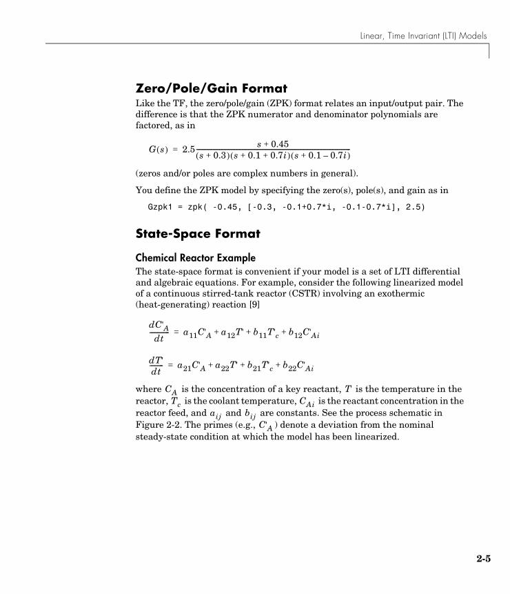
Zero/Pole/Gain FormatLike the TF, the zero/pole/gain (ZPK) format relates an input/output pair. The difference is that the ZPK numerator and denominator polynomials are factored, as in
(zeros and/or poles are complex numbers in general).
You define the ZPK model by specifying the zero(s), pole(s), and gain as in
Gzpk1 = zpk( -0.45, [-0.3, -0.1+0.7*i, -0.1-0.7*i], 2.5)
State-Space Format
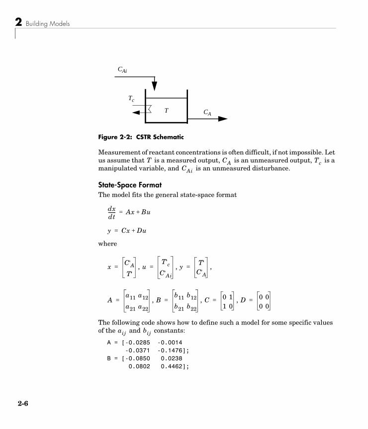
Chemical Reactor ExampleThe state-space format is convenient if your model is a set of LTI differential and algebraic equations. For example, consider the following linearized model of a continuous stirred-tank reactor (CSTR) involving an exothermic (heat-generating) reaction [9]
where is the concentration of a key reactant, is the temperature in the reactor, is the coolant temperature, is the reactant concentration in the reactor feed, and and are constants. See the process schematic in Figure 2-2. The primes (e.g., ) denote a deviation from the nominal steady-state condition at which the model has been linearized.
G s( ) 2.5 s 0.45+s 0.3+( ) s 0.1 0.7i+ +( ) s 0.1 0.7i–+( )
-----------------------------------------------------------------------------------------------------=
dC'Adt
------------- a11C'A a12T' b11T'c b12C'Ai+ + +=
dT'dt
--------- a21C'A a22T' b21T'c b22C'Ai+ + +=
CA TTc CAi
aij bijC'A
2 Building Models
2-6
Figure 2-2: CSTR Schematic
Measurement of reactant concentrations is often difficult, if not impossible. Let us assume that is a measured output, is an unmeasured output, is a manipulated variable, and is an unmeasured disturbance.
State-Space FormatThe model fits the general state-space format
where
, , ,
, , ,
The following code shows how to define such a model for some specific values of the and constants:
A = [-0.0285 -0.0014 -0.0371 -0.1476];B = [-0.0850 0.0238 0.0802 0.4462];
Tc
CAi
CAT
T CA TcCAi
dxdt------- Ax Bu+=
y Cx Du+=
x C'AT'
= uT'c
C'Ai
= y T'C'A
=
Aa11 a12
a21 a22
= Bb11 b12
b21 b22
= C 0 11 0
= D 0 00 0
=
aij bij

Linear, Time Invariant (LTI) Models
2-7
C = [0 1 1 0];D = zeros(2,2);CSTR = ss(A,B,C,D);
This defines a continuous-time state space model (no sampling period has been specified, so it defaults to zero). You can also specify discrete-time state space models and add delays to either type. See the Control System Toolbox documentation for details.
LTI Object PropertiesThe ss function in the last line of the above code creates a state space model, CSTR, which is an LTI object. The tf and zpk commands described in sections “Transfer Function Format” on page 2-4 and “Zero/Pole/Gain Format” on page 2-5 also create LTI objects. Such objects contain the model parameters as well as optional properties.
LTI Properties for the CSTR ExampleThe following code sets some of the CSTR model’s optional properties:
CSTR.InputName = {'T_c', 'C_A_i'};CSTR.OutputName = {'T', 'C_A'};CSTR.StateName = {'C_A', 'T'};CSTR.InputGroup.MV = 1;CSTR.InputGroup.UD = 2;CSTR.OutputGroup.MO = 1;CSTR.OutputGroup.UO = 2;CSTR
The first three lines specify labels for the input, output and state variables. The next four specify the signal type for each input and output. The designations MV, UD, MO, and UO mean manipulated variable, unmeasured disturbance, measured output, and unmeasured output. (See “Plant Inputs and Outputs” on page 2-3 for definitions of these terms.) For example, the code specifies that input 2 of model CSTR is an unmeasured disturbance. The last line causes the LTI object to be displayed, generating the following lines in the MATLAB Command Window:

2 Building Models
2-8
a = C_A T C_A -0.0285 -0.0014 T -0.0371 -0.1476 b = T_c C_Ai C_A -0.085 0.0238 T 0.0802 0.4462
c = C_A T T 0 1 C_A 1 0 d = T_c C_Ai T 0 0 C_A 0 0 Input groups: Name Channels MV 1 UD 2 Output groups: Name Channels MO 1 UO 2 Continuous-time model
Input and Output NamesThe optional InputName and OutputName properties affect the model displays, as in the above example. The Model Predictive Control Toolbox also uses the InputName and OutputName properties to label plots and tables. In that context, the underscore character causes the next character to be displayed as a subscript.

Linear, Time Invariant (LTI) Models
2-9
Input and Output Types
General Case. As mentioned in “Overview” on page 2-2, the Model Predictive Control Toolbox supports three input types and two output types. In an Model Predictive Control Toolbox design, designation of the input and output types determines the controller dimensions and has other important consequences.
For example, suppose your plant structure were as follows:
The resulting controller would have four inputs (the three MOs and the MD) and two outputs (the MVs). It would include feedforward compensation for the measured disturbance, and would assume that you wanted the unmeasured disturbances and outputs to be included as part of the regulator design.
If you didn’t want a particular signal to be treated as one of the above types, you could do one of the following:
• Eliminate the signal before using the model in controller design.
• For an output, designate it as unmeasured, then set its weight to zero (see “Output Weights” on page 3-22).
• For an input, designate it as an unmeasured disturbance, then define a custom state estimator that ignores the input (see “Disturbance Modeling and Estimation” on page 3-32).
Plant Inputs Plant Outputs
Two manipulated variables (MV) Three measured outputs (MO)
One measured disturbance (MD) Two unmeasured outputs (UO)
Two unmeasured disturbances (UD)

2 Building Models
2-10
Note By default, the Model Predictive Control Toolbox assumes that unspecified plant inputs are manipulated variables, and unspecified outputs are measured. Thus, if you didn’t specify signal types in the above example, the controller would have four inputs (assuming all plant outputs were measured) and five outputs (assuming all plant inputs were manipulated variables).
Example. For model CSTR, the default Model Predictive Control Toolbox assumptions are incorrect. You must set its InputGroup and OutputGroup properties, as illustrated in the above code, or modify the default settings when you load the model into the design tool.
The Model Predictive Control Toolbox provides a “helper function” called setmpcsignals to make type definition more convenient. For example
CSTR = setmpcsignals(CSTR, 'UD', 2, 'UO', 2);
sets InputGroup and OutputGroup to the same values as in the previous example. The CSTR display would then include the following lines:
Input groups: Name Channels Unmeasured 2 Manipulated 1
Output groups: Name Channels Unmeasured 2 Measured 1
Notice that setmpcsignals sets unspecified inputs to Manipulated and unspecified outputs to Measured.
See the Control System Toolbox documentation for additional information on LTI object properties.

Linear, Time Invariant (LTI) Models
2-11
Multiinput Multioutput (MIMO) PlantsMost Model Predictive Control Toolbox applications involve plants having multiple inputs and outputs. Model CSTR described in “State-Space Format” on page 2-5 is a MIMO plant, and the state space format extends naturally from single-input single-output (SISO) to MIMO plants.
You can also use the tf and zpk functions to build a MIMO plant model. For example, consider the following model of a distillation column [11], which has been used in many advanced control studies:
Outputs y1 and y2 represent measured product purities. The control objective is to hold each at specified setpoints. To do so, the controller manipulates inputs u1 and u2, the flow rates of reflux and reboiler steam, respectively. Input u3 is a measured feed flow rate disturbance.
The model consists of six transfer functions, one for each input/output pair. Each transfer function is the first-order-plus-delay form often used by process control engineers.
The following code shows how to define the distillation column model for use in the Model Predictive Control Toolbox:
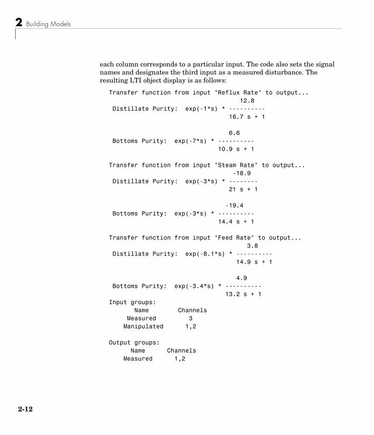
g11 = tf( 12.8, [16.7 1], 'IOdelay', 1.0);g12 = tf(-18.9, [21.0 1], 'IOdelay', 3.0);g13 = tf( 3.8, [14.9 1], 'IOdelay', 8.1);g21 = tf( 6.6, [10.9 1], 'IOdelay', 7.0);g22 = tf(-19.4, [14.4 1], 'IOdelay', 3.0);g23 = tf( 4.9, [13.2 1], 'IOdelay', 3.4);DC = [g11 g12 g13 g21 g22 g23];DC.InputName = {'Reflux Rate', 'Steam Rate', 'Feed Rate'};DC.OutputName = {'Distillate Purity', 'Bottoms Purity'};DC = setmpcsignals(DC, 'MD', 3)
The code defines the individual transfer functions, and then forms a matrix in which each row contains the transfer functions for a particular output, and
y1
y2
12.8e s–
16.7s 1+------------------------ 18.9e 3s––
21.0s 1+------------------------- 3.8e 8.1s–
14.9s 1+------------------------
6.6e 7s–
10.9s 1+------------------------ 19.4e 3s––
14.4s 1+------------------------- 4.9e 3.4s–
13.2s 1+------------------------
u1
u2
u3
=
2 Building Models
2-12
each column corresponds to a particular input. The code also sets the signal names and designates the third input as a measured disturbance. The resulting LTI object display is as follows:
Transfer function from input "Reflux Rate" to output... 12.8 Distillate Purity: exp(-1*s) * ---------- 16.7 s + 1 6.6 Bottoms Purity: exp(-7*s) * ---------- 10.9 s + 1 Transfer function from input "Steam Rate" to output... -18.9 Distillate Purity: exp(-3*s) * -------- 21 s + 1 -19.4 Bottoms Purity: exp(-3*s) * ---------- 14.4 s + 1 Transfer function from input "Feed Rate" to output... 3.8 Distillate Purity: exp(-8.1*s) * ---------- 14.9 s + 1 4.9 Bottoms Purity: exp(-3.4*s) * ---------- 13.2 s + 1Input groups: Name Channels Measured 3 Manipulated 1,2 Output groups: Name Channels Measured 1,2

Linear, Time Invariant (LTI) Models
2-13
LTI Model CharacteristicsThe Control System Toolbox provides functions for analyzing LTI models. Some of the more commonly used are listed below. Type the example code at the MATLAB prompt to see how they work for the CSTR example.
Example Intended Result
dcgain(CSTR) Calculate gain matrix for the CSTR model’s input/output pairs.
impulse(CSTR) Graph CSTR model’s unit-impulse response.
ltiview(CSTR) Open the LTI Viewer with the CSTR model loaded. You can then display model characteristics by making menu selections.
pole(CSTR) Calculate CSTR model’s poles (to check stability, etc.).
step(CSTR) Graph CSTR model’s unit-step response.
zero(CSTR) Compute CSTR model’s transmission zeros.

2 Building Models
2-14
System Identification Toolbox ModelsThe System Identification Toolbox for MATLAB generates LTI models based on plant input/output data. This section explains how to use such models in the Model Predictive Control Toolbox:
• “System Identification Model Definition Example” on page 2-14
• “Converting a System Identification Toolbox Model to an LTI Object” on page 2-15
• “Step-Response Models” on page 2-17
Note The System Identification Toolbox is an optional product. To determine whether your installation includes it, type ver at the MATLAB prompt, and look for “System Identification Toolbox” in the list of installed products.
System Identification Model Definition ExampleTo use the System Identification Toolbox, you first create an iddata object containing measured values of your plant input and output signals. The following example uses the System Identification Toolbox tutorial data set, a temperature-control application. Load the data as follows:
load dryer2
This creates vectors u2 and y2 in your workspace. Vector u2 is a sequence of 1000 plant input values (electrical power), and y2 is the corresponding output sequence (1000 temperature values). The sampling period is 0.08 second.
Create an iddata object called dry as follows:
dry = iddata(y2,u2,0.08);
Once the data has been loaded, use the System Identification Toolbox GUI or commands to determine a model that best fits the data. For example, the commands
dry.InputName = 'Power';dry.OutputName = 'Temperature';ze = detrend(dry(1:300));m1 = pem(ze);

System Identification Toolbox Models
2-15
create a System Identification Toolbox model called m1 (see the System Identification Toolbox documentation for a detailed explanation). If you type
whos m1
at the MATLAB prompt, the displayed result is
Name Size Bytes Class
m1 4-D 22470 idss object
Notice that m1 is an idss object, one of seven possible System Identification Toolbox model types (idgrey, idarx, idpoly, idproc, idss, idmodel, idfrd). The pem function settings govern the type of model generated.
Like other System Identification Toolbox objects, m1 defines a model structure and adjustable parameter values that best fit the data. It also contains System Identification-Toolbox-specific information, such as the algorithm used to estimate the parameters.
Converting a System Identification Toolbox Model to an LTI ObjectOnce you’ve created a System Identification Toolbox model based on your data, you must convert it to a standard LTI object prior to using it in the Model Predictive Control Toolbox. The System Identification Toolbox provides a special conversion function (ss).
Note An exception is the mpc function described in “Controller Definition” on page 4-2, which can use System Identification Toolbox models directly.
Creating an LTI State-Space ModelUse the ss function to convert a System Identification Toolbox model object (except the idfrd type) to a standard Control System Toolbox ss (state-space) object, which is the form used internally by the Model Predictive Control Toolbox. For example,
m1ss = ss(m1)

2 Building Models
2-16
converts m1, an System Identification Toolbox object, to m1ss, an LTI ss object, and displays the following:
a = x1 x2 x3 x1 0.9492 -0.2127 0.03679 x2 0.2599 0.6523 0.2342 x3 -0.04822 -0.6639 0.1393
b = Power v@Temperatur x1 -0.0005008 0.002613 x2 -0.01335 -0.0002421 x3 -0.06729 -0.004463 c = x1 x2 x3 Temperature 14.09 -0.108 -0.08164
d = Power v@Temperatur Temperature 0 0.03968 Input groups: Name Channels Measured 1 Noise 2 Sampling time: 0.08Discrete-time model
We see that m1ss is a 3rd-order, discrete-time, state-space model with a sampling time of 0.08, one output (“Temperature”), and two inputs (“Power” and “v@Temperatur”).
Noise InputsThe System Identification Toolbox automatically creates a noise input for each output to model the impact of unmeasured disturbances and measurement

System Identification Toolbox Models
2-17
noise. In the above example, there is one output (Temperature). Its associated noise input is v@Temperatur.
The System Identification Toolbox designates the noise inputs using the LTI model’s InputGroup property. In the above example, channel 2 (v@Temperatur) is classified as Noise, while channel 1 (Power) is Measured.
When you use such a model in the Model Predictive Control Toolbox, Noise inputs will be treated as unmeasured disturbances, and Measured inputs will be treated as manipulated variables. (See “Overview” on page 2-2 for discussion of input types.) If these defaults are inappropriate, you must correct them prior to using the model in a design. If you are using the design tool, “Loading a Plant Model” on page 3-3 shows how to specify signal types. When using commands, you need to set the models InputGroup and OutputGroup properties, as illustrated in “LTI Object Properties” on page 2-7.
Note As discussed in “Disturbance Modeling and Estimation” on page 3-32, unmeasured disturbance inputs influence the default controller design. A System Identification Toolbox model of its Noise inputs might fit the given data, but another experiment might yield a very different noise model. If a controller designed using such a model seems to work well during setpoint changes but is slow to eliminate disturbances or exhibits steady-state error, try modifying the Model Predictive Control Toolbox disturbance modeling settings.
Step-Response ModelsEarly predictive control implementations used finite step-response or finite impulse-response models, often called nonparametric LTI models (see [6] for example). Such models are easy to determine from plant data ([3], [7]) and they have intuitive appeal.
The System Identification Toolbox includes tools for nonparametric model identification. See its documentation for details.
For example, given the iddata object ze (defined in “System Identification Model Definition Example” on page 2-14), you could type
m2 = step(ze);

2 Building Models
2-18
This identifies a finite step-response model, m2, which is a System Identification Toolbox idarx object. Then typing
step(m2)
would display its unit-step response.
You could convert m2 to an LTI object for use in Model Predictive Control Toolbox design (see “Creating an LTI State-Space Model” on page 2-15). The disadvantage is that the model will be high-order, especially if your plant is MIMO. For example, converting m2 generates a ss object of order 69.
High-order models can degrade certain Model Predictive Control Toolbox operations, such as estimator design. As is the case with most recent predictive control implementations (see [5] for example), the Model Predictive Control Toolbox algorithms work best with a low-order parametric model. For example, reference [10] describes a systematic approach that identifies a step-response model as an intermediate step. The System Identification Toolbox documentation also advocates this approach.

Using Simulink to Develop LTI Models
2-19
Using Simulink to Develop LTI ModelsThe LTI and System Identification Toolbox models discussed in the previous sections are linear dynamic models. Most real systems are nonlinear. If you’d like to simulate Model Predictive Control Toolbox control of a nonlinear system, you must model the plant in Simulink.
Although a Model Predictive Control Toolbox controller can regulate a nonlinear plant, the model used within the controller must be linear. In other words, the controller employs a linear approximation of the nonlinear plant. The accuracy of this approximation is a key issue affecting controller performance.
This raises the question: how to obtain the approximation? The usual approach is to linearize the nonlinear plant at a specified operating point. The Simulink environment provides two ways to accomplish this:
• “Linearization Using Simulink Control Design” on page 2-19
• “Linearization Using Simulink Functions” on page 2-24
Linearization Using Simulink Control DesignSimulink Control Design is an optional product that supports model linearization. To determine whether or not your license includes it, type ver at the MATLAB prompt, and note whether or not “Simulink Control Design” appears in the resulting product list.
The Simulink Control Design documentation includes extensive background on linearization and several examples. You can linearize a Simulink model of the plant alone, or a model that includes both the plant and its controller.
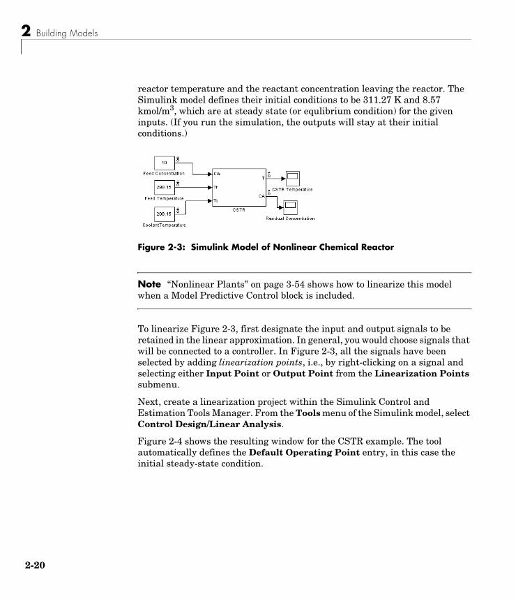
Figure 2-3 is a Simulink model of a continuous stirred-tank reactor (CSTR). It is similar to the one in Figure 2-2, except that here the model is nonlinear and includes an additional input: the feed temperature. This code is stored in the Model Predictive Control Toolbox demo folder. You can open it by typing
CSTR_OL
at the MATLAB prompt.
As shown in Figure 2-3, the three inputs are being held at constant values: 10 kmol/m3 for the feed concentration, and 298.15 K for the feed and coolant temperatures. Like the model of Figure 2-2, there are two state variables: the
2 Building Models
2-20
reactor temperature and the reactant concentration leaving the reactor. The Simulink model defines their initial conditions to be 311.27 K and 8.57 kmol/m3, which are at steady state (or equlibrium condition) for the given inputs. (If you run the simulation, the outputs will stay at their initial conditions.)
Figure 2-3: Simulink Model of Nonlinear Chemical Reactor
Note “Nonlinear Plants” on page 3-54 shows how to linearize this model when a Model Predictive Control block is included.
To linearize Figure 2-3, first designate the input and output signals to be retained in the linear approximation. In general, you would choose signals that will be connected to a controller. In Figure 2-3, all the signals have been selected by adding linearization points, i.e., by right-clicking on a signal and selecting either Input Point or Output Point from the Linearization Points submenu.
Next, create a linearization project within the Simulink Control and Estimation Tools Manager. From the Tools menu of the Simulink model, select Control Design/Linear Analysis.
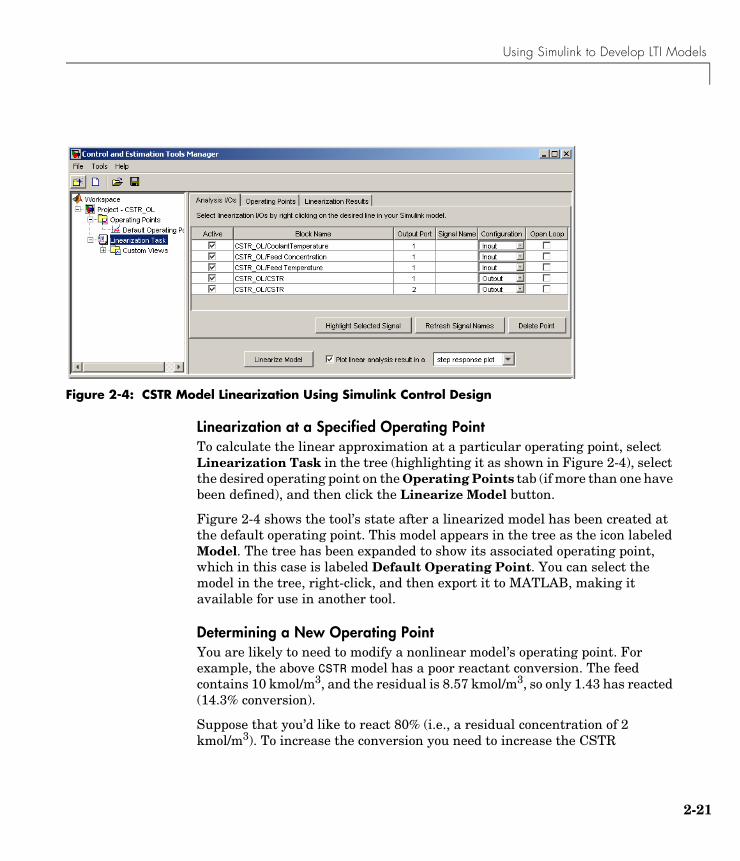
Figure 2-4 shows the resulting window for the CSTR example. The tool automatically defines the Default Operating Point entry, in this case the initial steady-state condition.
Using Simulink to Develop LTI Models
2-21
Figure 2-4: CSTR Model Linearization Using Simulink Control Design
Linearization at a Specified Operating PointTo calculate the linear approximation at a particular operating point, select Linearization Task in the tree (highlighting it as shown in Figure 2-4), select the desired operating point on the Operating Points tab (if more than one have been defined), and then click the Linearize Model button.
Figure 2-4 shows the tool’s state after a linearized model has been created at the default operating point. This model appears in the tree as the icon labeled Model. The tree has been expanded to show its associated operating point, which in this case is labeled Default Operating Point. You can select the model in the tree, right-click, and then export it to MATLAB, making it available for use in another tool.
Determining a New Operating PointYou are likely to need to modify a nonlinear model’s operating point. For example, the above CSTR model has a poor reactant conversion. The feed contains 10 kmol/m3, and the residual is 8.57 kmol/m3, so only 1.43 has reacted (14.3% conversion).
Suppose that you’d like to react 80% (i.e., a residual concentration of 2 kmol/m3). To increase the conversion you need to increase the CSTR

2 Building Models
2-22
temperature, but how much? Also, to change the CSTR temperature you need to change the coolant temperature, but how much?
One approach would be to change the coolant temperature, run a simulation of sufficient duration to reach a new steady state, check the final residual concentration, and repeat until you achieve the desired 2.0 kmol/m3 residual. This is tedious and essentially impossible in a more complex situation where you are trying to match several targets simultaneously.
Simulink Control Design can search for a new steady state operating point that achieves the desired conversion. First, you must modify the model so Simulink can change the coolant temperature. One way is to represent the coolant temperature with an Inport block, as shown below (compare to Figure 2-3, which uses a Constant block.
Save this modified model under a new name. Then from the Tools menu, select Control Design/Linear Analysis as before. If the Control and Estimation Tools Manager window containing CSTR_OL is still open (as shown in Figure 2-4), a new linearization project will be inserted. Otherwise, the window will open with CSTR_OL as a new project.
It will contain a default operating point. This is as before except that the coolant temperature appears as an input and defaults to zero. To modify this, select Operating Points in the tree, and select the Create Operating Points tab. On this panel, select the States tab and set the check boxes as shown below.

Using Simulink to Develop LTI Models
2-23
Also set the desired value of the second state (the residual concentration) to 2, as shown. You are asking for a new operating point in which one state is specified (known) and both are at steady state. The reactor temperature value (311.267) is an initial guess, and the tool uses optimization to find the value that satisfies all the specifications.
Next, click the Inputs tab and verify that the coolant temperature input is not specified (i.e., its Known check box is not selected) as shown below.
The value is an initial guess that will be changed. You can set it to 298, as shown above, to help the tool converge its trial-and-error calculations. (The default guess of 0 should also work here, but it is good practice to supply a guess to aid convergence.)
Finally, click the Compute Operating Point button at the panel bottom. A calculation progress panel shows the specification error at each iteration. When it’s finished, you should see the line, “Operating point specifications were successfully met” and a new operating point should appear in the tree. Click on

2 Building Models
2-24
this and observe that the required reactor temperature is 373.13 K, and the required coolant temperature is 305.20 K.
Let’s calculate a new linearized model at this condition, comparing it to that obtained at the original point. Suppose you exported the original model as Model1, and the other as Model2. The following command would compare their step responses:
step(Model1, Model2)
You should see some significant quantitative and qualitative differences, especially in the response to a change in feed concentration. At the original low-conversion state, increasing the feed concentration increases both the reactor temperature and the residual concentration. At high conversion, however, the reaction is more sensitive to temperature changes. Increasing the feed concentration causes an initial rise in the residual concentration, but the increased temperature accelerates the reaction rate and the residual concentration goes below its initial value. Thus, if one were trying to control conversion by adjusting the feed concentration, a model-based controller designed for low conversion would be certain to fail at high conversion.
Linearization Using Simulink FunctionsAnother approach is to linearize the model using standard Simulink functions. This is more restrictive: you cannot perform open loop analysis of the Simulink model, and the signals to be retained in the linearized model must be connected to an inport or outport block. On the other hand, Simulink Control Design is not needed.
The diagram below shows a modification of Figure 2-3 with three inport blocks designating the input signals (on the left-hand sided of the model) and two outports designating the outputs (on the right).

Using Simulink to Develop LTI Models
2-25
Suppose this model were named CSTR_INOUT. The linmod command linearizes it as follows:
[a,b,c,d]=linmod('CSTR_INOUT')
a =
-0.2505 1.9897 -0.0880 -1.1669
b =
0 1.0000 0.3000 1.0000 0 0
c =
1.0000 0 0 1.0000
d =
0 0 0 0 0 0
By default, linmod uses the initial conditions defined in the model as the operating point. Options allow you to specify an operating point. The command outputs are the standard state-space matrices defining an LTI model. You can use these to create an LTI model as follows:
cstr = ss(a,b,c,d)
2 Building Models
2-26
Bibliography[1] Allgower, F., and A. Zheng, Nonlinear Model Predictive Control, Springer-Verlag, 2000.
[2] Camacho, E. F., and C. Bordons, Model Predictive Control, Springer-Verlag, 1999.
[3] Cutler, C., and F. Yocum, “Experience with the DMC inverse for identification,” Chemical Process Control — CPC IV (Y. Arkun and W. H. Ray, eds.), CACHE, 1991.
[4] Kouvaritakis, B., and M. Cannon, Non-Linear Predictive Control: Theory & Practice, IEE Publishing, 2001.
[5] Maciejowski, J. M., Predictive Control with Constraints, Pearson Education POD, 2002.
[6] Prett, D., and C. Garcia, Fundamental Process Control, Butterworths, 1988.
[7] Ricker, N. L., “The use of bias least-squares estimators for parameters in discrete-time pulse response models,” Ind. Eng. Chem. Res., Vol. 27, pp. 343, 1988.
[8] Rossiter, J. A., Model-Based Predictive Control: A Practical Approach, CRC Press, 2003.
[9] Seborg, D. E., T. F. Edgar, and D. A. Mellichamp, Process Dynamics and Control, 2nd Edition, Wiley, 2004, pp. 34-36 and 94-95.
[10] Wang, L., P. Gawthrop, C. Chessari, T. Podsiadly, and A. Giles, “Indirect approach to continuous time system identification of food extruder,” J. Process Control, Vol. 14, Number 6, pp. 603-615, 2004.
[11] Wood, R. K., and M. W. Berry, Chem. Eng. Sci., Vol. 28, pp. 1707, 1973.

3
The Design Tool
Introduction (p. 3-2) Opens the design tool and navigates its views
Linear Simulations (p. 3-12) Defines and runs simulation scenarios
Changing Controller Settings (p. 3-19) Modifies the default controller settings for improved close-loop performance
Defining Soft Output Constraints (p. 3-40) Includes hard and soft output constraints in your controller specifications
Robustness Testing (p. 3-44) Tests sensitivity to prediction errors
Plant Models with Delays (p. 3-47) Defines controller settings for plants having delays
Nonsquare Plants (p. 3-52) Designs controllers for plants with unequal numbers of manipulated variables and outputs
Nonlinear Plants (p. 3-54) Works with Simulink models – linearization and nominal conditions
Saving Your Work (p. 3-65) Exports your controller design and saves your design specifications
Loading Your Saved Work (p. 3-67) Imports a controller and loads saved design specifications

3 The Design Tool
3-2
IntroductionThe Model Predictive Control Toolbox design tool is a graphical user interface for controller design. It operates under the Control and Estimation Tools Manager. (For another use of the Control and Estimation Tools Manager, see “Linearization Using Simulink Control Design” on page 2-19.)
This section covers the following topics:
• “Starting the Design Tool” on page 3-2
• “Loading a Plant Model” on page 3-3
• “Signal Property Specifications” on page 3-5
Starting the Design ToolStart the design tool by typing the MATLAB command
mpctool
The Control and Estimation Tools Manager window appears, as shown below. By default, it contains a Model Predictive Control Toolbox task called MPCdesign (listed in the tree view on the left side of the window), which is selected, causing the view shown on the right to appear.
Introduction
3-3
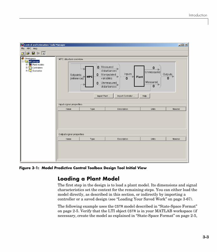
Figure 3-1: Model Predictive Control Toolbox Design Tool Initial View
Loading a Plant ModelThe first step in the design is to load a plant model. Its dimensions and signal characteristics set the context for the remaining steps. You can either load the model directly, as described in this section, or indirectly by importing a controller or a saved design (see “Loading Your Saved Work” on page 3-67).
The following example uses the CSTR model described in “State-Space Format” on page 2-5. Verify that the LTI object CSTR is in your MATLAB workspace (if necessary, create the model as explained in “State-Space Format” on page 2-5,

3 The Design Tool
3-4
and set its label and signal type properties as explained in “LTI Object Properties” on page 2-7).
Model Import DialogClick the Import Plant button in the design tool’s initial view (see Figure 3-1). The Plant Model Importer dialog appears.
Figure 3-2: Plant Model Importer Dialog
The Import from MATLAB Workspace radio button should be selected by default, as shown. The dialog section labeled Items in your Workspace lists your LTI models. If CSTR doesn’t appear, define it as discussed above, then reactivate the import dialog.
Once CSTR appears, select it. The dialog section labeled Properties then displays the number of inputs and outputs, their names and signal types, etc.
Click the Import button. This loads CSTR into the design tool. Then click the Close button (otherwise the dialog remains visible in case you want to import another model). The design tool should appear as in Figure 3-3.

Introduction
3-5
Figure 3-3: The Model Predictive Control Toolbox Design Tool’s Signal Definition View
Signal Property SpecificationsThe figure’s graphical display indicates that you’ve imported a plant model by showing the number of inputs and outputs, and the number in each subclass: measured disturbance, manipulated variables, etc.). Also, the tables labeled Input signal properties and Output signal properties fill with data:
• The Name entries are from the CSTR model’s InputName and OutputName properties (the design tool assigns defaults if necessary). You can edit these at any time.
3 The Design Tool
3-6
• The Type entries are from the CSTR model’s InputGroup and OutputGroup properties. (The design tool defaults all unspecified inputs to manipulated variables and all unspecified outputs to measured.)
Note Once you leave this view, if you subsequently change a signal type, you will have to restart the design. Be sure the signal types are correct at the beginning.
• The Description and Unit entries are optional. You can enter the values shown in Figure 3-3 manually. As you will see, the design tool uses them to label plots and other tables.
• The Nominal entries are initial conditions for simulations. The design tool default is 0.0.

Introduction
3-7
Navigation Using the Tree ViewThe tree in the left-hand frame of Figure 3-3 shows that the default MPCdesign node (see Figure 3-1) has been renamed CSTRcontrol by clicking on the name, waiting for the usual edit box to appear, typing the new name, and pressing Enter to finalize the choice.
Figure 3-3 also shows three new nodes below CSTRcontrol. These activate once you’ve imported a plant model (or controller).
In general, clicking a node displays a view supporting a particular design activity.
The Project View (Signal Properties Tables)For example, clicking the project node (CSTRcontrol in Figure 3-3) allows you to review and edit the signal properties tables.

3 The Design Tool
3-8
Listing Your Plant ModelsSelect the Plant models node to list the plant models you’ve imported, as shown in Figure 3-4. (Each model name is editable.) The Model details section displays properties of the selected model. There is also a space to enter notes describing the model’s special features. Buttons allow you to import a new model or delete one you no longer need.
Figure 3-4: Plant Models View with CSTR Model Selected
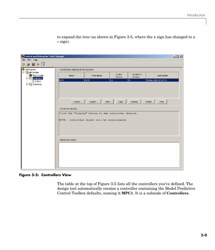
Viewing Your ControllersNext, select Controllers. The view shown in Figure 3-5 appears. A + sign to the left of Controllers indicates that it contains subnodes. You can click on a + sign
Introduction
3-9
to expand the tree (as shown in Figure 3-5, where the + sign has changed to a – sign).
Figure 3-5: Controllers View
The table at the top of Figure 3-5 lists all the controllers you’ve defined. The design tool automatically creates a controller containing the Model Predictive Control Toolbox defaults, naming it MPC1. It is a subnode of Controllers.

3 The Design Tool
3-10
Note If you define additional controllers, they will appear here. For example, you might want to test several options, saving each as a separate controller, making it easy to switch from one to another during testing.
The table Controllers defined in this project allows you to edit the controller name and gives you quick access to three important design parameters: Plant Model, Control Interval, and Prediction Horizon. All are editable, but leave them at their default values for this example.
The buttons shown in Figure 3-5 let you do the following:
• Import a controller designed previously and stored either in your workspace or in a MAT-file
• Export the selected controller to your workspace
• Create a new controller initialized to the Model Predictive Control Toolbox defaults
• Copy the selected controller, creating a duplicate you can modify
• Delete the selected controller
You can also right-click on the Controllers node to access menu options New, Import, and Export, or on one of its subnodes to access menu options Copy, Rename, Export, and Delete.
Select the MPC1 node to display the Model Predictive Control Toolbox default controller settings. (“Changing Controller Settings” on page 3-19 covers this view in detail).
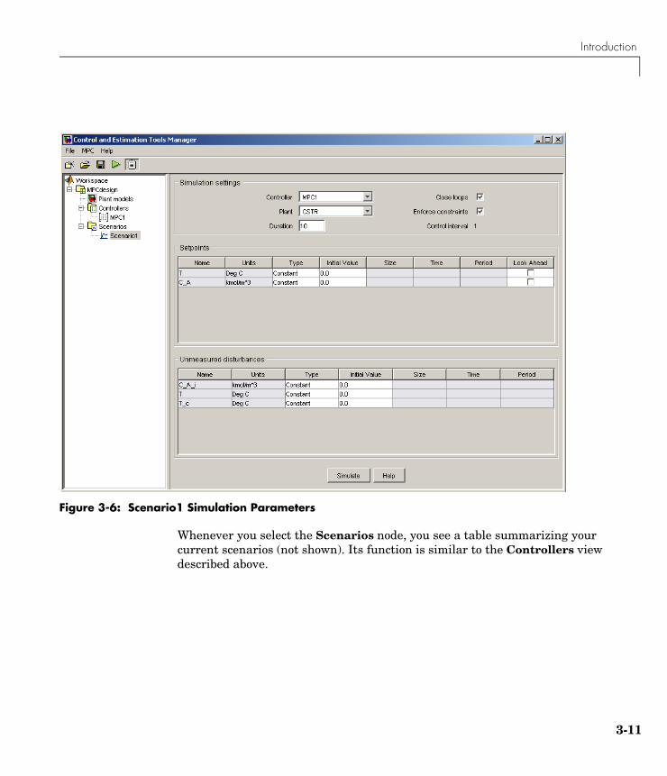
Viewing Simulation ScenariosA scenario is a set of conditions defining a simulation. The design tool creates a default scenario and names it Scenario1. To view it, click on the + symbol next to the Scenarios node, and select the Scenario1 subnode. You should see a view like that shown in Figure 3-6.
Introduction
3-11
Figure 3-6: Scenario1 Simulation Parameters
Whenever you select the Scenarios node, you see a table summarizing your current scenarios (not shown). Its function is similar to the Controllers view described above.
3 The Design Tool
3-12
Linear SimulationsYou will usually want to test your controller in simulations. The Model Predictive Control Toolbox design tool makes it easy to run closed-loop simulations involving a Model Predictive Control Toolbox controller and an LTI plant model. This plant can differ from that used in the controller design, allowing you to test your controller’s sensitivity to prediction errors (see “Robustness Testing” on page 3-44).
This section covers the following topics:
• “Defining Simulation Conditions” on page 3-12
• “Running a Simulation” on page 3-14
• “Open-Loop Simulations” on page 3-16
Defining Simulation ConditionsTo define simulation conditions, select an existing scenario node or create a new one, and then edit its tabular fields to define your conditions.
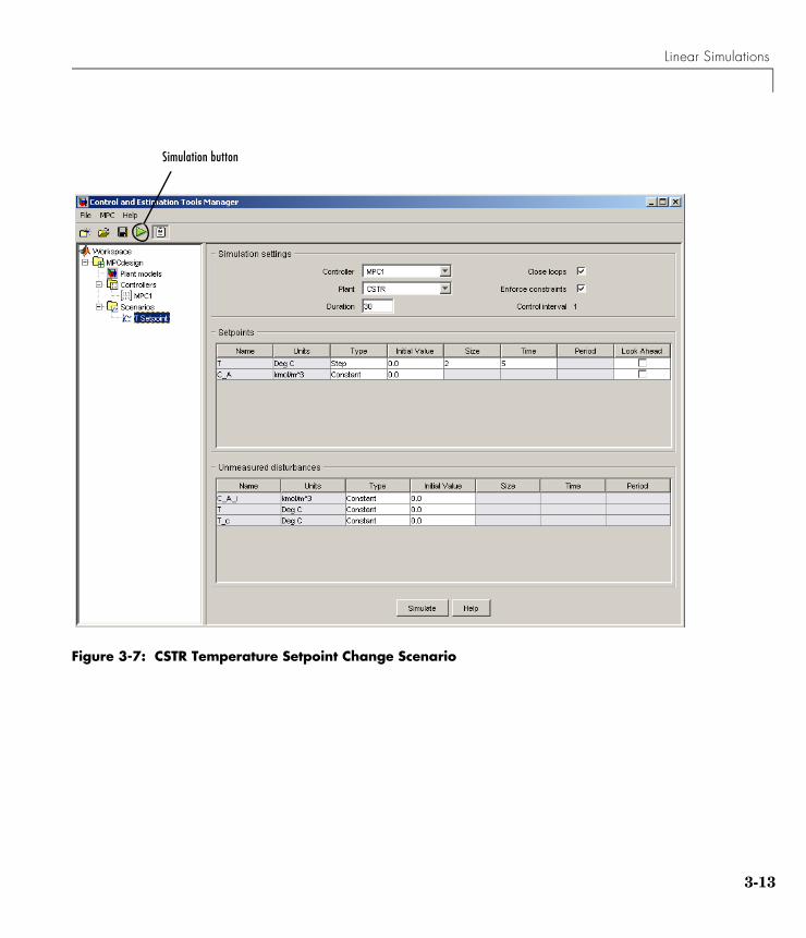
Figure 3-7 shows the result of renaming the default Scenario1 node to T Setpoint and editing its default conditions. The required editing steps are as follows:
• Increase Duration from 10 to 30
• Locate the tabular data defining the reactor temperature setpoint (first row of the upper table in Figure 3-7)
- Click the Type table cell and select Step from the list of choices
- Change Size from 1.0 to 2
- Change Time from 1.0 to 5
Note The Control Interval is a property of the controller being used (MPC1 in this case). To change it, select the controller node in the tree, and then edit the value on the Model and Horizons tab (see “Model and Horizons” on page 3-19). Such a change would apply to all simulations involving that controller.
Linear Simulations
3-13
Figure 3-7: CSTR Temperature Setpoint Change Scenario
Simulation button

3 The Design Tool
3-14
Running a SimulationTo run a simulation, do one of the following:
• Select the scenario you want to run, and click its Simulate button (see the bottom of Figure 3-7)
• Click the toolbar’s Simulation button, which is the triangular icon shown on the top left of Figure 3-7.
The toolbar method runs the current scenario, i.e., the one most recently selected or modified.
Try running the T Setpoint scenario. This should generate the two response plot windows shown in Figure 3-8 and Figure 3-9.
Figure 3-8: Plant Outputs for T Setpoint Scenario with Added Data Markers

Linear Simulations
3-15
Figure 3-9: Plant Inputs for T Setpoint Scenario
Figure 3-8 shows that the reactor temperature setpoint increases suddenly by 2 degrees at t = 5, as you specified when defining the scenario in the previous section. Unfortunately, the temperature does not track the setpoint very well, and there is a persistent error of about 1.6 degrees at the end of the simulation.
Also, the controller requests a sudden jump in the coolant temperature (see upper graph in Figure 3-9), which might be difficult to deliver in practice. (The lower graph in Figure 3-9 shows that the feed concentration, CAi, remains constant, as specified in the scenario.)
See “Changing Controller Settings” on page 3-19 for ways to overcome these deficiencies.
3 The Design Tool
3-16
Note Figure 3-8 has data markers. To add these, left-click on the curve to create the data marker. Drag a marker to relocate it. Left-click in a graph’s white space to erase its markers. For more information on data markers, see the Control System Toolbox documentation.
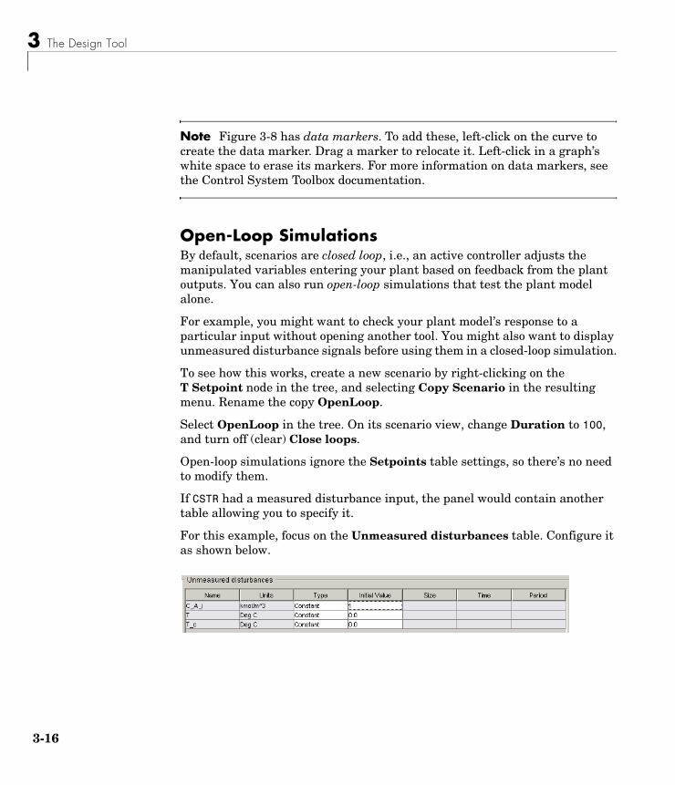
Open-Loop SimulationsBy default, scenarios are closed loop, i.e., an active controller adjusts the manipulated variables entering your plant based on feedback from the plant outputs. You can also run open-loop simulations that test the plant model alone.
For example, you might want to check your plant model’s response to a particular input without opening another tool. You might also want to display unmeasured disturbance signals before using them in a closed-loop simulation.
To see how this works, create a new scenario by right-clicking on the T Setpoint node in the tree, and selecting Copy Scenario in the resulting menu. Rename the copy OpenLoop.
Select OpenLoop in the tree. On its scenario view, change Duration to 100, and turn off (clear) Close loops.
Open-loop simulations ignore the Setpoints table settings, so there’s no need to modify them.
If CSTR had a measured disturbance input, the panel would contain another table allowing you to specify it.
For this example, focus on the Unmeasured disturbances table. Configure it as shown below.

Linear Simulations
3-17
The C_A_i input’s nominal value is 0.0 (see Figure 3-3), so the above models a sudden increase to 1 at the beginning of the simulation. The following is an equivalent setup using the Step type.
Using one of these, simulate the scenario (click its Simulate button). The output response plot should be as shown below.
This is the CSTR model’s open-loop response to a unit step in the CAi disturbance input.
You could also set up the table as shown below.

3 The Design Tool
3-18
This simulation would display the open-loop response to a unit step in the Tc manipulated variable input (try it).
Finally, set it up as follows.
This adds a pulse to the T output. The pulse begins at time t = 10, and lasts 20 time units. Its height is 0.95 degrees.
Run the simulation. The output response plot displays the pulse (see Figure 3-10). In this case, the T output’s nominal value is zero, so you only see the pulse. (If the T output had a nonzero nominal value, the pulse would add to that.)
Figure 3-10: Response Plot Showing Open Loop Pulse Disturbance
If you were to run a closed-loop simulation with this same T disturbance, the controller would attempt to hold T at its setpoint, and the result would differ from that shown in Figure 3-10.

Changing Controller Settings
3-19
Changing Controller SettingsThe simulations shown in Figure 3-8 and Figure 3-9 used the default controller settings. These often work well, but the CSTR application is an exception. The following discussion covers the main controller options in more detail, and shows how to tune a controller for better performance.
This section covers the following topics:
• “Model and Horizons” on page 3-19
• “Weight Tuning” on page 3-21
• “Blocking” on page 3-26
• “Defining Manipulated Variable Constraints” on page 3-29
• “Disturbance Modeling and Estimation” on page 3-32
Model and HorizonsSelect your MPC1 controller in the tree. The view shown in Figure 3-11 should appear. If necessary, select the Model and Horizons tab to bring it to the front. This tab contains the following controller options:
• Plant model specifies the LTI model to be used for controller predictions.
• Control interval sets the elapsed time between successive adjustments of the controller’s manipulated variables.
• Prediction horizon is the number of control intervals over which the outputs are to be optimized.
• Control horizon sets the number of control intervals over which the manipulated variables are to be optimized.
• Selecting the Blocking option gives you more control over the way in which the controller’s moves are allocated.
Leave all of the Model and Horizons tab settings at their default values for now.

3 The Design Tool
3-20
Figure 3-11: Controller Options — Models and Horizons Tab

Changing Controller Settings
3-21
Weight TuningSelect the Weight Tuning tab. The view shown in Figure 3-12 appears.
Figure 3-12: Controller Options — Weight Tuning Tab
Make the following changes (already done in the above view):
• In the Input weights table, change the coolant temperature’s Rate weight from the default 0.1 to 0.3.
• In the Output weights section, change the reactant concentration’s Weight (last entry in second row) from the default 1.0 to 0.
Test these changes using the T Setpoint scenario (click the toolbar’s Simulation button). Figure 3-13 shows that the CSTR temperature now tracks

3 The Design Tool
3-22
the setpoint change smoothly, reaching the new value in about 10 time units with no overshoot.
Figure 3-13: Improved Setpoint Tracking for CSTR Temperature
On the other hand, the reactant concentration, CA, exhibits a larger deviation from its setpoint, which is being held constant at zero (compare to Figure 3-8, where the final deviation is about a factor of 4 smaller).
This behavior reflects an unavoidable trade-off. The controller has only one adjustment at its disposal: the coolant temperature. Therefore, it can’t satisfy setpoints on both outputs.
Output WeightsThe output weights let you dictate the accuracy with which each output must track its setpoint. Specifically, the controller predicts deviations for each output over the prediction horizon. It multiplies each deviation by the output’s weight value, and then computes the weighted sum of squared deviations,
, as followsSy k( )
Sy k( ) wyj rj k i+( ) yj k i+( )–[ ]
⎩ ⎭⎨ ⎬⎧ ⎫
2
j 1=
ny
∑i 1=
P
∑=

Changing Controller Settings
3-23
where k is the current sampling interval, k+i is a future sampling interval (within the prediction horizon), P is the number of control intervals in the prediction horizon, ny is the number of plant outputs, is the weight for output j, and the term is a predicted deviation for output j at interval k+1.
The weights must be zero or positive. If a particular weight is large, deviations for that output dominate . One of the controller’s objectives is to minimize . Thus, a large weight on a particular output causes the controller to minimize deviations in that output (relative to outputs having smaller weights).
For example, the default values used to produce Figure 3-8 specify equal weights on each output, so the controller is trying to eliminate deviations in both, which is impossible. On the other hand, the design of Figure 3-13 uses a weight of zero on the second output, so it is able to eliminate deviations in the first output.
Note The second output is unmeasured. Its predictions rely on the plant model and the temperature measurements. If the model were reliable, we could hold the predicted concentration at a setpoint, allowing deviations in the reactor temperature instead. In practice, it would be more common to control the temperature as done here, using the predicted reactant concentration as an auxiliary indicator.
You might expect equal output weights to result in equal output deviations at steady state. Figure 3-8 shows that this is not the case. The reason is that the controller is trying to satisfy several additional objectives simultaneously.
Rate WeightsOne such simultaneous objective is to minimize the weighted sum of controller adjustments, calculated according to
where M is the number of intervals in the control horizon, nmv is the number of manipulated variables, is the predicted adjustment in
wjy
rj k i+( ) yj k i+( )–[ ]
Sy k( )Sy k( )
S∆u k( ) wj∆u∆uj k i 1–+( )
⎩ ⎭⎨ ⎬⎧ ⎫
2
j 1=
nmv
∑i 1=
M
∑=
∆uj k i 1–+( )

3 The Design Tool
3-24
manipulated variable j at future (or current) sampling interval , and is the weight on this adjustment, called the rate weight because it
penalizes the incremental change rather than the cumulative value. Increasing this weight forces the controller to make smaller, more cautious adjustments.
Figure 3-14: Plant Inputs for Modified Rate Weight
k i 1–+wj
∆u

Changing Controller Settings
3-25
Figure 3-14 shows that increasing the rate weight from 0.1 to 0.3 decreases the move sizes significantly, especially the initial move (compare to Figure 3-9).
Setting the rate weight to 0.1 yields a faster approach to the T setpoint with a small overshoot, but the initial Tc move is about six times larger than needed to achieve the new steady state, which would be unacceptable in most applications (not shown; try it).
Note The controller minimizes the sum . Changes in the coolant temperature have unequal effects on the two outputs, so the steady-state output deviations won’t be equal, even when both output weights are unity as in Figure 3-8.
Input WeightsThe controller also minimizes the weighted sum of manipulated variable deviations from their nominal values, computed according to
where is the input weight and is the nominal value for input j. In the above simulations, you used the default, . This is the usual choice.
When a sustained disturbance or setpoint change occurs, the manipulated variable must deviate permanently from its nominal value (as shown in Figure 3-9 and Figure 3-14). Using a nonzero input weight forces the corresponding input back toward its nominal value. Test this by running a simulation in which you set the input weight to 1. The final Tc value is closer to its nominal value, but this causes T to deviate from the new setpoint (not shown).
Sy k( ) S∆u k( )+
Su k( ) wju uj k i 1–+( ) uj–[ ]
⎩ ⎭⎨ ⎬⎧ ⎫
2
j 1=
nmv
∑i 1=
M
∑=
wju uj
wju 0=

3 The Design Tool
3-26
Note Some applications involve more manipulated variables than plant outputs. In such cases, it is common to define nonzero input weights on certain manipulated variables in order to hold them near their most economical values. The remaining manipulated variables eliminate steady-state error in the plant outputs.
BlockingThe section “Weight Tuning” on page 3-21 used penalty weights to shape the controller’s response. This section covers the following topics:
• An alternative to penalty weighting, called blocking
• Side-by-side controller comparisons
To begin, select Controllers in the tree, and click the New button, creating a controller initialized to the Model Predictive Control Toolbox default settings. Rename this controller Blocking 1 by editing the appropriate table cell.
Select Blocking 1 in the tree, select its Weight Tuning tab, and set the Weight for output C_A to 0 (see “Weight Tuning” on page 3-21 to review the reason for this). Leave other weights at their defaults.
Now select the Model and Horizons tab, and select its Blocking check box. This activates the blocking options. It also deactivates the Control Horizon option (the blocking options override it).
Set Number of moves computed per step to 2. Verify that Blocking allocation within prediction horizon is set to Beginning, the default.
Select Controllers in the tree, and use its Copy button to create two controllers based on Blocking 1. Rename these Blocking 2 and Blocking 3. Edit their blocking options, setting Blocking allocation within prediction horizon to Uniform for Blocking 2, and to End for Blocking 3.
Select Scenarios in the tree. Rename the T Setpoint scenario to T Setpoint 1, and set its Controller option to Blocking 1.
Create two copies of T Setpoint 1, naming them T Setpoint 2 and T Setpoint 3. Set their Controller options to Blocking 2 and Blocking 3,
Changing Controller Settings
3-27
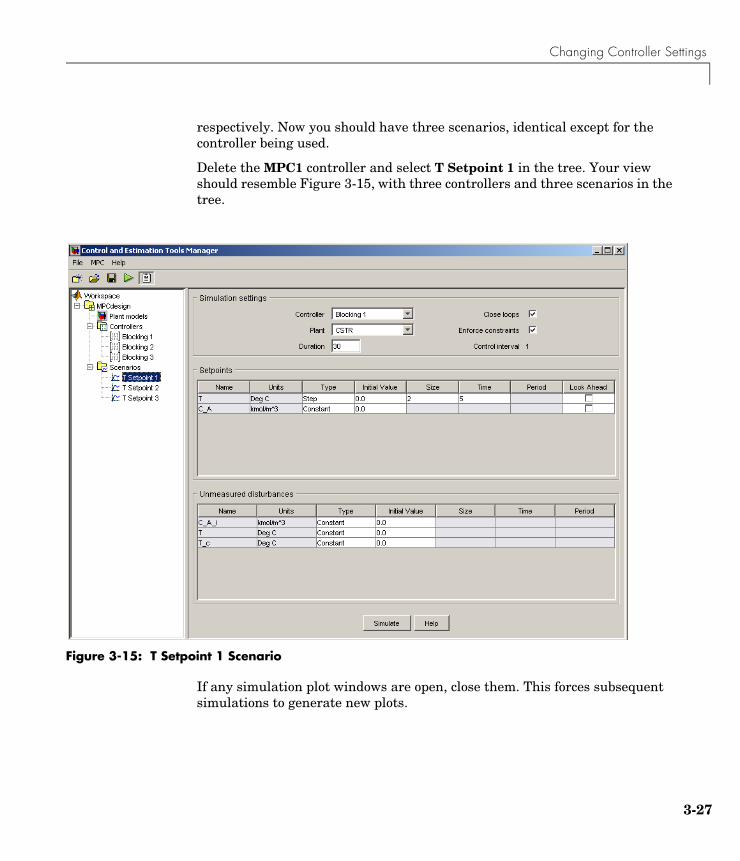
respectively. Now you should have three scenarios, identical except for the controller being used.
Delete the MPC1 controller and select T Setpoint 1 in the tree. Your view should resemble Figure 3-15, with three controllers and three scenarios in the tree.
Figure 3-15: T Setpoint 1 Scenario
If any simulation plot windows are open, close them. This forces subsequent simulations to generate new plots.

3 The Design Tool
3-28
Simulate each of the three scenarios. When you run the first, new plot windows open. Leave them open when you run the other two scenarios so all three results appear together, as shown in Figure 3-16 and Figure 3-17.
Figure 3-16: Blocking Comparison, Outputs
Figure 3-17: Blocking Comparison, Manipulated Variable
The numeric annotations on these figures refer to the three scenarios. Recall that T Setpoint 1 uses the default blocking, which usually results in faster setpoint tracking but larger manipulated variable moves. The blocking options in T Setpoint 2 and T Setpoint 3 reduce the move size but make setpoint tracking more sluggish.

Changing Controller Settings
3-29
Results for T Setpoint 3 are very similar to those shown in Figure 3-13 and Figure 3-14, where a penalty rate weight reduced the move sizes. If rate weights and blocking achieve the same ends, why does the Model Predictive Control Toolbox provide both features? One difference not evident in this simple problem is that blocking applies to all the manipulated variables in your application, but each rate weight affects one only.
Note To obtain the dashed lines shown for T Setpoint 2, activate the plot window and select Property Editor from the View menu. The Property Editor appears at the bottom of the window. Then select the curve you want to edit. The Property Editor lets you change the line type, thickness, color, and symbol type. Select the axis labels to see additional options.
By default, the Model Predictive Control Toolbox plots each scenario on the same plot. If you recalculate a revised scenario, it replots that result but doesn’t change any others.
If you don’t want to see a particular scenario, right-click on the plot and use the Responses menu option to hide it. (You can also close the plot window and recalculate selected responses in a fresh window.)
Defining Manipulated Variable ConstraintsPhysical devices have limited ranges and rates of change. For example, the CSTR model’s coolant might be restricted to a 20 degree range (from -10 to 10) and its maximum rate of change might be degrees per control interval. If these are true physical restrictions, it’s good practice to include them in the controller design. Otherwise the controller might attempt an unrealistic adjustment.
To compare constrained and unconstrained performance for the CSTR example, select the Blocking 1 controller in the tree, and rename it Unconstrained.
Select its Model and Horizons tab and turn off (clear) its Blocking option. Increase Control horizon to 3, and reduce Control Interval to 0.25.
Delete the Blocking 2 and Blocking 3 controllers. (Click Yes or OK to dismiss the resulting warning messages.)
4±

3 The Design Tool
3-30
Copy the Unconstrained controller. Name this copy MVconstraints, and select its Constraints tab. Then enter the manipulated variable constraints shown in Figure 3-18.
Figure 3-18: Entering CSTR Manipulated Variable Constraints
If any simulation plot windows are open, close them (to force fresh plots).
Select the T Setpoint 1 scenario. If necessary, set its Controller option to Unconstrained. Change Duration to 15, and simulate the scenario.
Select the T Setpoint 2 scenario, set its Controller option to MVconstraints, change its Duration to 15, and simulate it. The results appear in Figure 3-19 and Figure 3-20.
The larger control horizon and smaller control interval cause the unconstrained controller to make larger moves (see Figure 3-20, curve 1). The output settles at the new setpoint in about 5 time units rather than the 10 required previously (compare curve 1 in Figure 3-19 to curve 1 in Figure 3-16).
Figure 3-20 (curve 2) shows that the Max Up Rate constraint limits the size of the first two moves to 4 degrees. The third move hits the Maximum constraint at 10 degrees. The coolant temperature remains saturated at its upper limit for the next 7 control intervals, then slowly moves back down to its final value.
Figure 3-19 (curve 2) shows that the output response is slower, but still settles at the new setpoint smoothly within about 5 time units. This demonstrates the anti-windup protection provided automatically by the Model Predictive Control Toolbox controller.

Changing Controller Settings
3-31
Figure 3-19: CSTR Outputs, Unconstrained (1) and MVconstraints (2)
Figure 3-20: CSTR Manipulated Variable, Unconstrained (1) and MVconstraints (2)
3 The Design Tool
3-32
Disturbance Modeling and EstimationThe previous sections tested the controller’s response to setpoint changes. In process control, disturbances rejection is often more important. The Model Predictive Control Toolbox allows you to tailor the controller’s disturbance response. The following example assumes that you have just completed the above section, and the design tool is still open.
Select the first controller in the tree and rename it InputSteps. (Its settings should be identical to the Unconstrained controller of the previous section.)
Copy this controller. Rename the copy OutputSteps. Select its Estimation tab. The initial view should be as in Figure 3-21. Note the following:
• The Model Predictive Control Toolbox default settings are being used. (The Use Model Predictive Control Defaults button restores these settings if you modify them.)
• The Output disturbances tab is selected, and the Signal-by-signal option is on. The graphic shows that the output disturbances add to each output.
• The tabular entries show, however, that these disturbance magnitudes are currently zero.

Changing Controller Settings
3-33
Figure 3-21: Default Output Disturbance Settings for CSTR

3 The Design Tool
3-34
Select the Input disturbances tab. (This would be inactive if the plant model had no unmeasured disturbances.) The view should change to that shown in CFigure 3-22.
Figure 3-22: Default Input Disturbance Settings for CSTR
In this case the disturbance magnitude is nonzero, and the disturbance type is Steps. Thus, the controller assumes that disturbances enter as random steps (integrated white noise) at the plant’s unmeasured disturbance input.
Select the Measurement noise tab, verifying that the controller is assuming white noise, magnitude 1 (not shown).
The following summarizes the Model Predictive Control Toolbox default disturbance modeling assumptions for this case:
• Additive output disturbances: none
Changing Controller Settings
3-35
• Unmeasured input disturbances: random steps (integrated white noise)
• Measurement noise: white
In general, if your plant model includes unmeasured disturbance inputs, the Model Predictive Control Toolbox default strategy will assume that they are dominant and sustained, as in the above example. This forces the controller to include an integrating mode, intended to eliminate steady-state error.
If the plant model contains no unmeasured input disturbances, the Model Predictive Control Toolbox assumes sustained (integrated white noise) disturbances at the measured plant outputs.
If there are more measured outputs than unmeasured input disturbances, it assumes sustained disturbances in both locations according to an algorithm described in the Model Predictive Control Toolbox online documentation.
In any case, the design tool displays the assumptions being used.
To modify the estimation strategy in the OutputSteps controller, do the following:
• Select the Input disturbances tab. Set the disturbance Type to White, and its Magnitude to 0.
• Select the Output disturbances tab. For the T output, set the disturbance Type to Steps, and its magnitude to 1.
This reverses the default assumptions, i.e., the OutputSteps controller assumes that sustained disturbances enter at the plant output rather than at the unmeasured disturbance input. The InputSteps controller is still using the original (default) assumptions.
Next, select the first scenario in the tree. Rename it Disturbance 1, set its Duration to 30, define all setpoints as constant zero values, and define a unit-step disturbance in the unmeasured input, C_A_i. If necessary, set its Controller option to InputSteps. Figure 3-23 shows the final Disturbance 1 scenario.
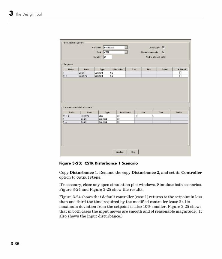
3 The Design Tool
3-36
Figure 3-23: CSTR Disturbance 1 Scenario
Copy Disturbance 1. Rename the copy Disturbance 2, and set its Controller option to OutputSteps.
If necessary, close any open simulation plot windows. Simulate both scenarios. Figure 3-24 and Figure 3-25 show the results.
Figure 3-24 shows that default controller (case 1) returns to the setpoint in less than one third the time required by the modified controller (case 2). Its maximum deviation from the setpoint is also 10% smaller. Figure 3-25 shows that in both cases the input moves are smooth and of reasonable magnitude. (It also shows the input disturbance.)

Changing Controller Settings
3-37
The default controller expects unmeasured disturbances to enter as defined in the scenarios, so it’s not surprising that the default controller performs better. The main message here is that the difference can be large, so it merits design consideration.
Figure 3-24: CSTR Outputs for Disturbance Scenarios 1 and 2

3 The Design Tool
3-38
Figure 3-25: CSTR Inputs for Disturbance Scenarios 1 and 2
For comparison, reset the two scenarios so that the only disturbance is a one-degree step increase added to the measured reactor temperature. The modified controller (case 2) is designed for such disturbances, and Figure 3-26 shows that it performs better, but the difference is less dramatic than in the previous scenario. The default controller is likely to be best if the real process has multiple dominant disturbance sources.
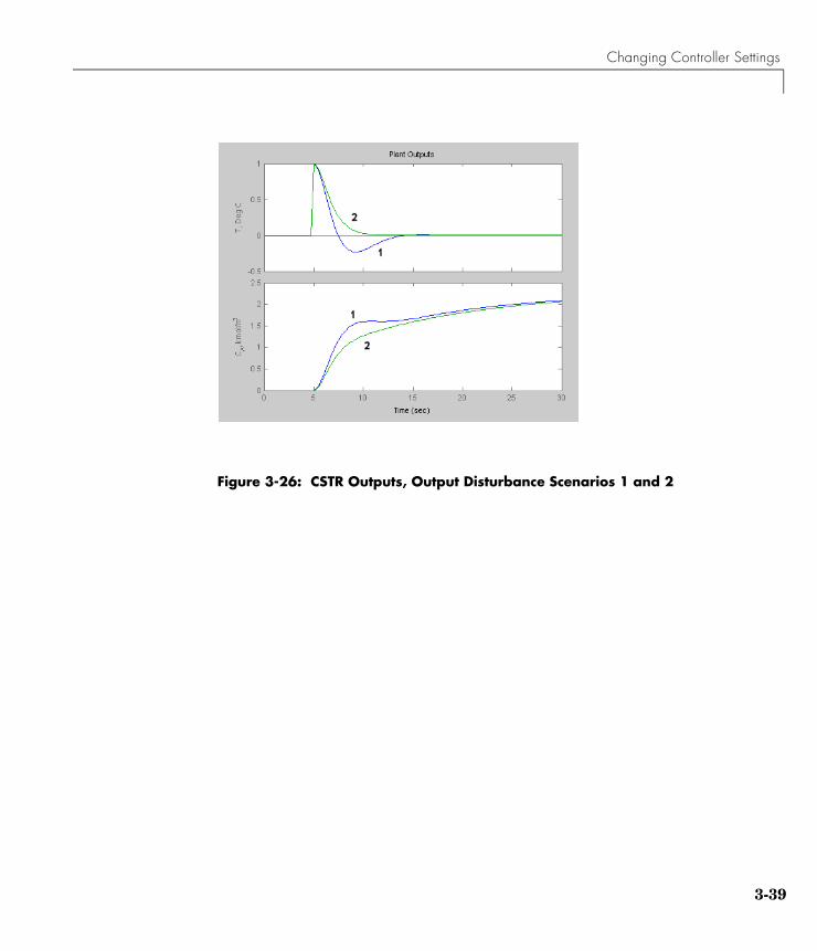
Changing Controller Settings
3-39
Figure 3-26: CSTR Outputs, Output Disturbance Scenarios 1 and 2
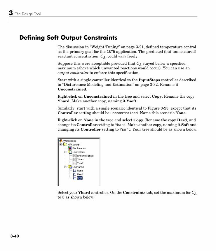
3 The Design Tool
3-40
Defining Soft Output ConstraintsThe discussion in “Weight Tuning” on page 3-21, defined temperature control as the primary goal for the CSTR application. The predicted (but unmeasured) reactant concentration, CA, could vary freely.
Suppose this were acceptable provided that CA stayed below a specified maximum (above which unwanted reactions would occur). You can use an output constraint to enforce this specification.
Start with a single controller identical to the InputSteps controller described in “Disturbance Modeling and Estimation” on page 3-32. Rename it Unconstrained.
Right-click on Unconstrained in the tree and select Copy. Rename the copy Yhard. Make another copy, naming it Ysoft.
Similarly, start with a single scenario identical to Figure 3-23, except that its Controller setting should be Unconstrained. Name this scenario None.
Right-click on None in the tree and select Copy. Rename the copy Hard, and change its Controller setting to Yhard. Make another copy, naming it Soft and changing its Controller setting to Ysoft. Your tree should be as shown below.
Select your Yhard controller. On the Constraints tab, set the maximum for CA to 3 as shown below.

Defining Soft Output Constraints
3-41
Click the Constraint Softening button to obtain the dialog shown in Figure 3-27. The Input constraints section shows the bounds on the inputs and their rates, and relaxation bands, which let you soften these constraints. By default, input constraints are hard, meaning that the controller tries to prevent any violation.
Figure 3-27: Constraint Softening Dialog
The Output constraints section lists the output limits and their relaxation bands. By default, the output constraints are soft. Make the CA upper limit hard by entering a zero as its relaxation band (as in Figure 3-27).
Select the Ysoft controller. Define a soft upper bound on CA by using the same settings shown in Figure 3-27, but with a relaxation band of 100 instead of 0.

3 The Design Tool
3-42
Simulate the three scenarios in the order they appear in the tree, i.e., None, Hard, Soft. The resulting output responses appear in Figure 3-28.
Figure 3-28: Constraint Softening Scenarios: 1 = None, 2 = Hard, 3 = Soft
Curve 1 is without output constraints, which is identical to curve 1 in Figure 3-24. This controller allows the CA output to vary freely, but the controlled temperature returns to its setpoint within 10 time units after the disturbance happens.
Curve 2 shows the behavior with a hard upper limit at CA = 3. Once CA reaches this bound, the controller must use its one manipulated variable (Tc) to satisfy the constraint, so it’s no longer able to control the temperature.
Curve 3 shows the result for a soft constraint. The controller reaches a compromise between the competing objectives: temperature control and constraint satisfaction. As you’d expect, performance lies between the curve 1 and curve 2 extremes.
The numerical value of the relaxation band represents a relative tolerance for constraint violations, not a strict limit (if it were the latter, it would be a hard constraint). If you were to increase its relaxation band (currently set at 100), performance would move toward Case 1, and vice versa.

Defining Soft Output Constraints
3-43
If you have multiple constraints, you can harden or soften them simultaneously using the slider at the bottom of the controller’s constraint softening dialog (see Figure 3-27).
In general, you’ll have to experiment to determine the settings that provide appropriate trade-offs for your application. In particular, the relaxation band settings interact with those on the controller’s Weight Tuning tab (see “Weight Tuning” on page 3-21).
Another important factor is the expected numerical range for each variable. For example, if a particular variable stays within of its nominal value, it should have a small relaxation band relative to another variable having a range of .
For details on the Model Predictive Control Toolbox constraint softening formulation, see the “Optimization Problem” section in the Model Predictive Control Toolbox online documentation.
0.1±
100±

3 The Design Tool
3-44
Robustness TestingIt’s good practice to test your controller’s sensitivity to prediction errors. Classical phase and gain margins are one way to quantify robustness for a SISO application. The Robust Control Toolbox and µ-Analysis and Synthesis Toolbox provide sophisticated approaches for MIMO systems. It can also be helpful to run simulations. The following example illustrates the simulation approach.
Plant Model PerturbationUse the following code to create a perturbed version of the CSTR model:
CSTRp = CSTR;CSTRp.a=[-0.0303 -0.0113 -0.0569 -0.1836];CSTRp.b=[-0.0857 0.0191 0.1393 0.4241];
This creates a copy of CSTR called CSTRp, then replaces the state space A and B matrices with perturbed versions (compare to the originals defined in “State-Space Format” on page 2-5). Use the following command to compare the two step responses:
step(CSTR, CSTRp)
Observe the difference in the responses (not shown).
Select Plant models in the tree. Click the Import button and import the CSTRp model.
Simulation TestsDelete all controllers except the first one in the tree. If necessary, make its settings identical to Unconstrained (see “Defining Manipulated Variable Constraints” on page 3-29).
Delete all scenarios except the first, naming that Accurate Model. Define its properties as shown in Figure 3-29. The scenario begins with a step change in the temperature setpoint, followed 25 time units later by a step disturbance in the reactant entering the CSTR.

Robustness Testing
3-45
Copy Accurate Model. Rename the copy Perturbed Model, and set its Plant option to CSTRp. Thus, both scenarios use the same controller, which is based on the CSTR model, but the Perturbed Model scenario uses a different model to represent the “real” plant. This tests the controller’s robustness to a change in plant parameters.
Figure 3-29: Robustness Test, Accurate Plant Model Scenario
Simulate the two scenarios. Figure 3-30 shows the output responses. As expected, setpoint tracking degrades when the model is inaccurate, but performance is still acceptable.
The disturbance rejection appears to improve with the perturbed model. This is a consequence of the perturbations used. The gain for the T/CAi output/input pair is about 15% smaller in the CSTRp model, which has two beneficial effects: the actual impact of the disturbance is reduced, and the controller is aggressive because it expects a larger impact.

3 The Design Tool
3-46
Figure 3-30: Robustness Test, Accurate Model (1) and Perturbed Model (2)
Note MIMO applications are usually more sensitive to model error than SISO applications, so robustness testing is especially recommended for MIMO cases.

Plant Models with Delays
3-47
Plant Models with DelaysUnlike many controller design approaches, the Model Predictive Control Toolbox can deal directly with models that include delays. A typical example is the distillation column model, DC, introduced in “Multiinput Multioutput (MIMO) Plants” on page 2-11. It includes a delay in each input/output channel.
You don’t need to approximate the delays in order to use this model in the Model Predictive Control Toolbox. On the other hand, the presence of delays will influence controller performance, and your controller specifications should account for them. The following example provides some guidelines and covers the following topics:
• “Importing the Plant Model” on page 3-47
• “Specifying Controller Horizons” on page 3-48
Importing the Plant ModelBefore continuing, the DC model must be in your workspace. (See “Multiinput Multioutput (MIMO) Plants” on page 2-11 for the commands needed to create it.)
Start the Model Predictive Control Toolbox design tool (type mpctool at the MATLAB command line). Import the DC model (see “Loading a Plant Model” on page 3-3).
Select Plant models in the tree. The DC model should be the only one listed. Scroll the Model details view to show the last few lines, which should appear as in Figure 3-31.
Figure 3-31: DC Model Details, Maximum Delay Values

3 The Design Tool
3-48
Specifying Controller HorizonsThe model’s maximum I/O delay is 6.7 minutes. It is good practice to specify the prediction and control horizons such that
where P is the prediction horizon, M is the control horizon, td,max is the maximum delay, and is the control interval.
Select MPC1 (the default controller name) in the tree. Select the Model and Horizons tab, and set Control interval to 1, a reasonable choice if the closed loop response time is to be of order 5-10 minutes.
Given the amount of plant delay and the specified control interval, the default horizons, P = 10, M = 2, would be a poor choice. Instead, set Prediction horizon to 30, and Control horizon to 5.
Select Scenario1 in the tree. Set Duration to 50. Define a constant setpoint of 1 for the first output (the distillate purity). Define a step increase of 1 in the second output’s setpoint, occurring at t = 25. All other signals should be zero. Simulate the scenario. Figure 3-32 and Figure 3-33 show the results.
Figure 3-32: DC Setpoint Response Scenario, Outputs
P M– td max, ∆t⁄»
∆t
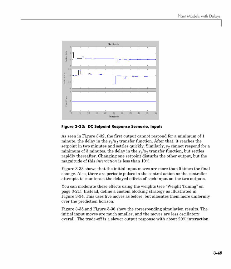
Plant Models with Delays
3-49
Figure 3-33: DC Setpoint Response Scenario, Inputs
As seen in Figure 3-32, the first output cannot respond for a minimum of 1 minute, the delay in the y1/u1 transfer function. After that, it reaches the setpoint in two minutes and settles quickly. Similarly, y2 cannot respond for a minimum of 3 minutes, the delay in the y2/u2 transfer function, but settles rapidly thereafter. Changing one setpoint disturbs the other output, but the magnitude of this interaction is less than 10%.
Figure 3-33 shows that the initial input moves are more than 5 times the final change. Also, there are periodic pulses in the control action as the controller attempts to counteract the delayed effects of each input on the two outputs.
You can moderate these effects using the weights (see “Weight Tuning” on page 3-21). Instead, define a custom blocking strategy as illustrated in Figure 3-34. This uses five moves as before, but allocates them more uniformly over the prediction horizon.
Figure 3-35 and Figure 3-36 show the corresponding simulation results. The initial input moves are much smaller, and the moves are less oscillatory overall. The trade-off is a slower output response with about 20% interaction.
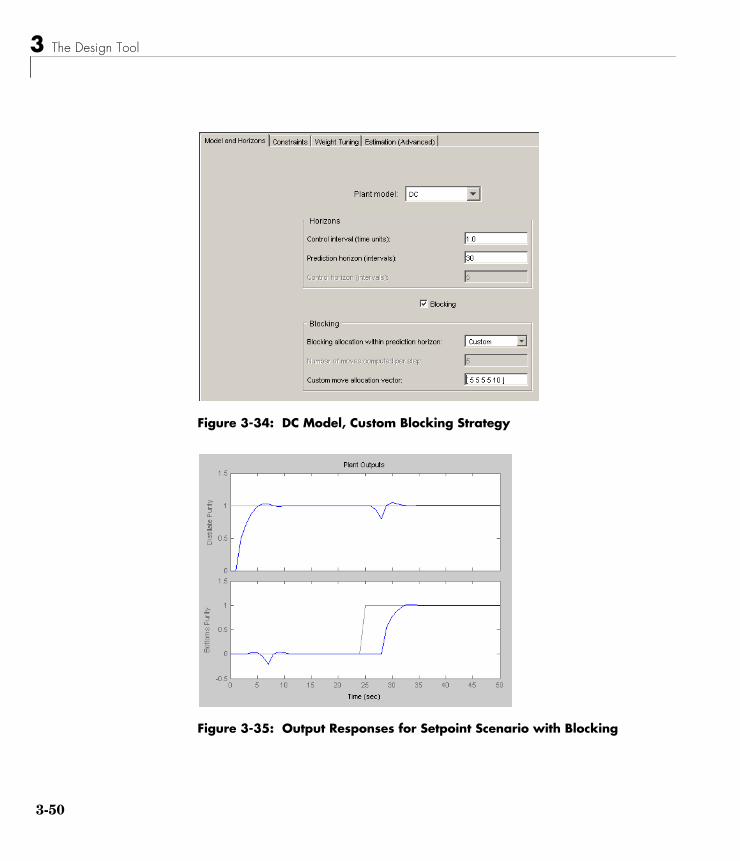
3 The Design Tool
3-50
Figure 3-34: DC Model, Custom Blocking Strategy
Figure 3-35: Output Responses for Setpoint Scenario with Blocking

Plant Models with Delays
3-51
Figure 3-36: Input Moves for Setpoint Scenario with Blocking

3 The Design Tool
3-52
Nonsquare PlantsA nonsquare plant has an unequal number of manipulated variables and output variables. This is common in practice, and the Model Predictive Control Toolbox supports an excess of manipulated variables or outputs. In such cases you will usually need to modify the default Model Predictive Control Toolbox settings.
This section covers the following topics:
• “More Outputs Than Manipulated Variables” on page 3-52
• “More Manipulated Variables Than Outputs” on page 3-53
More Outputs Than Manipulated VariablesWhen there are excess outputs, it is impossible to hold all of them at setpoints. You have the following options:
1 Enforce setpoints on all outputs, in which case all will deviate from their setpoints to some extent.
2 Specify that certain outputs need not be held at setpoints by setting their weights to zero on the controller’s Weight tuning tab.
The initial test of the CSTR controller used option 1 (the default), which caused both outputs to deviate from their setpoints (see Figure 3-8). You can adjust the offset in each output by changing the output weights. Increasing an output weight decreases the offset in that output (at the expense of increased offset in other outputs).
The modified CSTR controller used option 2 (see the discussion in “Weight Tuning” on page 3-21). In general, if the application has Ne more outputs than manipulated variables, setting Ne output weights to zero should allow the remaining outputs to be held at setpoints (unless the manipulated variables are constrained). This was the case for the modified CSTR controller (see Figure 3-13).
Outputs that have been “sacrificed” by setting their weights to zero can still be useful. If measured, they can help the controller to estimate the plant’s state, thereby improving its predictions. They can also be used as indicators, or as variables to be held within an operating region defined by output constraints.

Nonsquare Plants
3-53
More Manipulated Variables Than OutputsIn this situation, the default Model Predictive Control Toolbox settings should provide offset-free output-setpoint tracking, but the manipulated variables are likely to drift.
One way to avoid this is to use manipulated variable setpoints. If there are Ne excess manipulated variables and you hold Ne of them at target values, the rest should not drift. Rather, they will attain the values needed to eliminate output offset.
To define a manipulated variable setpoint, do the following:
1 Enter the setpoint value in the Nominal field in the signal properties view – see Figure 3-3
2 Assign a nonzero input weight using the Weight entry on the controller’s Weight tuning tab – see Figure 3-12
In step 2, the magnitude of the input weight determines the extent to which the manipulated variable can deviate from its target during a transient. See “Input Weights” on page 3-25 for more discussion and mathematical details.
You might want to allow such deviations temporarily in order to provide better output setpoint tracking. In that case, use a relatively small input weight. If you want the manipulated variable to stay near its target value at all times, increase its input weight.
Another way to avoid drift is to constrain one or more manipulated variables to a narrow operating region. You can even hold an MV constant by setting its lower and upper bounds to the same value (in which case its nominal value should also be set to this value), or by setting both of its rate constraints to zero. To define constraints, use the controller’s Constraints tab (see “Defining Manipulated Variable Constraints” on page 3-29).

3 The Design Tool
3-54
Nonlinear PlantsThe Model Predictive Control Toolbox provides a Simulink block you can use to control a plant modeled in Simulink. This section illustrates the procedure using the nonlinear CSTR model introduced earlier (see “Using Simulink to Develop LTI Models” on page 2-19). It covers the following topics:
• “The MPC Controller Block” on page 3-54
• “Initiating the Controller Design” on page 3-55
• “Validating the Linearized Model” on page 3-57
• “Modifying the Linearized Model” on page 3-59
• “Linear Simulation Tests” on page 3-60
• “Nonlinear Simulation Tests” on page 3-62
• “Modifying the Controller Using the Design Tool” on page 3-64
• “Exiting the Design Tool” on page 3-64
The MPC Controller BlockFigure 3-37 shows CSTR with an added MPC Controller block. (The model is called CSTR_MPC.mdl in the Model Predictive Control Toolbox demos folder.) The intent is to hold the residual concentration at a setpoint by adjusting the coolant temperature. The feed concentration and temperature inputs are disturbances, and the reactor temperature is an auxiliary, uncontrolled output. The concentration has a setpoint (reference), currently fixed at 8.57.
Figure 3-37: Simulink Model for CSTR Control

Nonlinear Plants
3-55
Note If you have the Model Predictive Control Toolbox and Simulink installed, the MPC Controller block appears in your Simulink block library. If necessary, see the Simulink documentation for details on how to use library blocks to construct a model.
Initiating the Controller DesignOnce you’ve installed an MPC Controller block in your Simulink model, as in Figure 3-37, you need to configure it. Click on it to open its block mask, shown below.
Figure 3-38: MPC Controller Block Mask
You must define the MPC controller parameter. All others are optional. Uncheck the box Enable input port for measured disturbance, as there are none in this case.

3 The Design Tool
3-56
If you had used the design tool to create a controller and had saved it in your workspace, you could type its name in the MPC controller box and you’d be ready to test it.
Instead, create the controller using the MPC Toolbox design tool. Click the Design button. A dialog (not shown) asks you to enter the number of manipulated variables, which are the plant inputs the controller can adjust to achieve its objectives. The coolant temperature is the only manipulated variable, so enter 1 and click OK.
The progress window shown below appears to mark the completion of each controller initialization step.
They are as follows:
1 Open the Control and Estimation Tools Manager, and install a project having the same name as the Simulink model (CSTR_MPC in this case).
2 Install a linearization task within the project and determine the plant’s I/O points, i.e., the signals connected to the MPC Controller block’s mv (manipulated variable) and mo (measured output) ports.
3 Determine a default operating point. This requires assumptions that might be incorrect, as demonstrated in the next section. In particular, the default outputs are zero.
4 Calculate a linearized plant model at this operating point using the linearization tool in Simulink Control Design (see “Linearization Using

Nonlinear Plants
3-57
Simulink Control Design” on page 2-19). The controller is open loop during this step, so it involves only the blocks between the plant inputs and outputs (as determined in step 2).
5 Install a Model Predictive Control Toolbox design task in the project, use the linearized model from step 4 to define a default controller (named MPC1), and enter its name as the block mask’s MPC controller parameter.
When the last step has been completed, click OK to close the progress window.
Validating the Linearized ModelAutomatic linearization requires assumptions that might be incorrect. You should always validate a linearized model before using it in a controller.
As shown below, the controller task is the MPC Controller node, the name of the corresponding Simulink block.
Note In general, a Simulink model can contain multiple controllers, in which case the project would include multiple controller design tasks, each with a unique name.
Start by examining the default operating point. Expand the tree until it appears as above, and then select Operating Point. The States tab should be active as shown (if not, click on it).

3 The Design Tool
3-58
By default, the Simulink Control Design linearization tool tries to find a steady-state point, i.e., it sets the Desired dx column to zero. As shown above, the Actual dx column contains a value that is far from zero.
Next, click the Outputs tab. By default, the linearization tool sets the desired plant output to zero. In the CSTR, this would require 100% conversion of the reactant, which is impossible, and the Outputs tab confirms that the desired values were not achieved.
Finally, export the linearized model to your workspace. Right-click on the MPC open loop plant 1 node and choose Export to obtain the dialog shown below.
Rename Linearized Model to Plant1 as shown above, clear the Operating Point check box (because there’s no reason to export it) and click OK. This exports the linearized model as an LTI object named Plant1.
At the MATLAB command line, type
step(Plant1)
You should obtain the following plot.

Nonlinear Plants
3-59
Thus, the linearized model predicts that a unit step increase in the coolant temperature will decrease the residual concentration, which is qualitatively correct. (Increasing the coolant temperature increases the reactor temperature. This increases the reaction rate, and the residual concentration decreases.)
The predicted magnitude is very small, however: of order 10−6. It should be of order 10−2 (you can verify this by removing the controller block from the diagram and running an open-loop step-response simulation). The assumption of zero plant outputs used to generate the default operating point are the cause. If this incorrect model were used in the controller, the coolant-temperature adjustments would be far too large, probably resulting in unstable behavior.
Modifying the Linearized ModelTherefore, the next step is to define a reasonable operating point and calculate a corresponding linearized model.
In the navigation tree, click the MPC Controller node. Notice that the nominal input and output signal values are zero by default. As discussed in “Linearization Using Simulink Control Design” on page 2-19, a coolant temperature of 298.15 K is the steady state for the plant’s initial condition (with the residual concentration at 8.57). Thus, in the Input signal properties

3 The Design Tool
3-60
table, set the coolant temperature’s nominal value to 298.15, as shown below, and in the Output signal properties table, set the concentration’s nominal value to 8.57. Also assign more descriptive signal names, as shown.
Click the Import Plant button to obtain the Plant Model Importer dialog. Then do the following:
1 Select the Linearized Plant from Simulink tab.
2 Change the Linearization model name to Plant2.
3 Select Create a new operating condition from MPC I/O values, and then click OK. A new model node named Plant2 and its operating point will appear within your design task.
4 Expand the Controllers node to expose the MPC1 node and select it. On its Model and Horizons pane, set Plant model to Plant2. This replaces the default (invalid) model with the modified one.
Leave the other controller settings at their default values.
Linear Simulation TestsIt’s good practice to test a controller in linear simulations before trying it on the nonlinear plant. Expand the Scenarios node and select Scenario1. Set Plant to Plant2, and set Duration to 40. Finally, define a step increase of 0.5 units in the concentration setpoint starting at time t = 1, as shown below.

Nonlinear Plants
3-61
Click the scenario’s Simulate button. This linear test predicts a smooth, rapid approach to the new setpoint with minimal overshoot, as shown below.
The corresponding coolant temperature adjustments are reasonable (not shown). If anything, you might want to make the controller more aggressive by adjusting its tuning weights (see “Weight Tuning” on page 3-21).
Note This plant’s steady-state gain is of order 0.01. Therefore, the default tuning weights lead to a relatively sluggish response. In general, you must adjust the tuning weights to compensate for the plant’s natural input/output response magnitudes.
You can also run tests to verify that the controller responds rapidly to either of the two unmeasured disturbances (not shown).

3 The Design Tool
3-62
Nonlinear Simulation TestsThe controller seems to be performing well in linear tests, so try it with the nonlinear plant. As will be demonstrated below, the design tool makes it easy to run a simulation, change the controller design if performance is unsatisfactory, and retest.
In the CSTR_MPC model window, change the concentration setpoint to 9.07. This simulates a 0.5-unit step increase in the setpoint at time t = 0. Run the Simulink simulation. The MPC Controller block automatically obtains the most recent MPC1 definition from the design tool. If necessary, open the model’s concentration scope block. The result should be as shown below.
The nonlinear response is more sluggish than the linear prediction. The controller reduces the coolant temperature to about 284.6 K (verify this by opening the model’s coolant temperature scope), whereas the linear simulation predicts a reduction to 289.4 K. In other words, when plant moves in this direction, the linearized model’s gain is too large. Still, the concentration goes to the setpoint rapidly.
Next, set the concentration setpoint to 8.07, i.e., a step-change of equal magnitude in the opposite direction. Run the simulation to obtain the concentration scope response shown below.

Nonlinear Plants
3-63
In this direction, the response is underdamped. You can verify that the controller changes the coolant temperature to 304.1 K, an increase of 6.0 K (recall the decrease of 13.5 K when the change was in the opposite direction). In other words, the controller’s linear model underpredicts the effect of a coolant temperature increase. If the setpoint were reduced significantly, the closed-loop system would become unstable (try 7.0, for example).
Thus, the controller’s effective operating range is limited. If you wanted to operate at a low concentration, you’d need to determine a linearized model at that condition and use it to design another controller.
Note This is typical of strongly nonlinear plants. If you needed to operate a conventional controller over such a wide range, you might consider gain scheduling. Equivalently, you could define predictive controllers for several operating points and switch from one to another depending on the measured concentration (see “Simulations Involving Nonlinear Plants” on page 4-8 for an example of this).
For the tested range, however, the oscillations die out quickly. You can verify that the controller responds equally well to small, sustained disturbances (i.e.,
in feed concentration or in feed temperature.0.5± 3±

3 The Design Tool
3-64
Modifying the Controller Using the Design ToolKeeping the design tool open makes it easy to test controller modifications. Each time you run a Simulink simulation, the MPC Controller block automatically obtains the latest settings for its MPC controller parameter (MPC1 in the above tests).
It’s also easy to compare several controllers. Suppose you wanted to try a different control interval (the controller designed above uses a 1-second interval). Create a new controller by right-clicking on the design tool’s MPC1 controller node, and selecting Copy Controller in the menu. This creates a duplicate controller called MPC1_copy. Rename it MPC2. Select MPC2 in the tree, activate its Model and Horizons tab and set Control interval to 2.
Now return to the MPC Controller block mask (if necessary, double-click on the block to open the mask) and change MPC controller from MPC1 to MPC2. Run a simulation with a disturbance or setpoint change, and then display the Coolant Temperature scope. You should see that the controller is now making step-wise adjustments every 2 minutes. As would be expected, controller performance degrades with less frequent measurement feedback, but not much.
To restore the original controller, just change MPC2 to MPC1 in the block mask.
Exiting the Design ToolWhen you close the design tool, you’ll be prompted to save any projects you’ve created or edited. For details, see “Saving a Project” on page 3-66.
Once the design tool has closed, the MPC Controller block mask expects its controller object to be in your workspace. Thus, you’ll also be prompted to export such controller objects. You need to do this if you plan to run your Simulink model with the design tool closed.
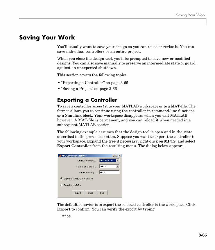
Saving Your Work
3-65
Saving Your WorkYou’ll usually want to save your design so you can reuse or revise it. You can save individual controllers or an entire project.
When you close the design tool, you’ll be prompted to save new or modified designs. You can also save manually to preserve an intermediate state or guard against an unexpected shutdown.
This section covers the following topics:
• “Exporting a Controller” on page 3-65
• “Saving a Project” on page 3-66
Exporting a ControllerTo save a controller, export it to your MATLAB workspace or to a MAT-file. The former allows you to continue using the controller in command-line functions or a Simulink block. Your workspace disappears when you exit MATLAB, however. A MAT-file is permanent, and you can reload it when needed in a subsequent MATLAB session.
The following example assumes that the design tool is open and in the state described in the previous section. Suppose you want to export the controller to your workspace. Expand the tree if necessary, right-click on MPC2, and select Export Controller from the resulting menu. The dialog below appears.
The default behavior is to export the selected controller to the workspace. Click Export to confirm. You can verify the export by typing
whos
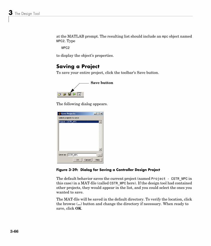
3 The Design Tool
3-66
at the MATLAB prompt. The resulting list should include an mpc object named MPC2. Type
MPC2
to display the object’s properties.
Saving a ProjectTo save your entire project, click the toolbar’s Save button.
The following dialog appears.
Figure 3-39: Dialog for Saving a Controller Design Project
The default behavior saves the current project (named Project - CSTR_MPC in this case) in a MAT-file (called CSTR_MPC here). If the design tool had contained other projects, they would appear in the list, and you could select the ones you wanted to save.
The MAT-file will be saved in the default directory. To verify the location, click the browse (...) button and change the directory if necessary. When ready to save, click OK.
Save button

Loading Your Saved Work
3-67
Loading Your Saved WorkThe following assumes that you’ve saved a project as described in the previous section. To reload this project, close the design tool if it’s open. Also clear any mpc objects from your workspace. (Type whos at the MATLAB prompt for a list of objects.) For example, if MPC1 and MPC2 are in your workspace, type
clear MPC1 MPC2
to clear (remove) them.
If you’ve closed the CSTR_MPC model, open it. (Figure 3-37 shows the model diagram). Double-click the MPC Controller block to open its mask, and verify that the MPC Controller parameter is set to MPC2.
Note If you were to attempt to run the CSTR_MPC model at this stage, an error dialog would indicate that the MPC Controller block was unable to initialize. The MPC2 object specified in the block mask must be loaded into your workspace or be part of an active design tool task.
You could define the required MPC2 object in one of the following ways:
• Import MPC2 from a MAT-file (assuming you had saved it as explained in “Exporting a Controller” on page 3-65).
• Load the model’s project file, which contains a copy of MPC2.
To use the second approach, open the design tool by typing
mpctool
in the Command Window. This creates a blank Model Predictive Control Toolbox project called MPCdesign. Click the Load button on the toolbar.
Load button

3 The Design Tool
3-68
This opens a dialog similar to that shown in Figure 3-39. Use it to select the project file you’ve saved, and then click OK to load the project. It should appear in the tree. Verify that it contains a controller named MPC2.
Run the CSTR_MPC model in Simulink. The block mask automatically retrieves MPC2 from the design tool, and the simulation runs. In other words, loading the project automatically restores the link between the design tool and the MPC Controller block.

4Using Model Predictive Control Toolbox Functions
Controller Definition (p. 4-2) Creates and modifies a controller using Model Predictive Control Toolbox functions
Linear Simulations (p. 4-6) Simulates the closed-loop response of a linear system that includes a Model Predictive Control Toolbox controller
Simulations Involving Nonlinear Plants (p. 4-8)
Uses functions for flexible, closed-loop simulation of systems with nonlinear plants.
Analysis Tools (p. 4-13) Analyzes Model Predictive Control Toolbox controllers

4 Using Model Predictive Control Toolbox Functions
4-2
Controller DefinitionChapter 3, “The Design Tool” showed how to use the Model Predictive Control Toolbox design tool to create a controller and test it. You might prefer to use functions instead. They allow access to options not available in the design tool, as well as automation of repetitive tasks using scripts and customized plotting.
This section covers the following topics:
• “Creating a Controller Object” on page 4-2
• “Viewing and Altering Controller Properties” on page 4-3
Creating a Controller ObjectThe following uses the CSTR model described in Chapter 2, “Building Models” as an example. To follow along, verify that the model’s LTI object is in your MATLAB workspace (if necessary, create it as explained in “Chemical Reactor Example” on page 2-5, and set its label and signal type properties as explained in “LTI Properties for the CSTR Example” on page 2-7).
The mpc function is the starting point for controller design. For example, type
Ts = 1;MPCobj = mpc(CSTR, Ts);
to create a controller based on the CSTR model with a control interval of 1 time unit, and all other parameters at their default values.
Note MPCobj is an mpc object. It contains a complete controller as defined by the Model Predictive Control Toolbox.
To display the controller’s properties, type
display(MPCobj)
or type the object’s name without a trailing semicolon.

Controller Definition
4-3
Viewing and Altering Controller PropertiesOnce you’ve defined an mpc object, it’s easy to alter its properties. For a description of the editable properties, type
mpcprops
To display the list of properties and their current values, type
get(MPCobj)
which in this case displays
ManipulatedVariables (MV): [1x1 struct] OutputVariables (OV): [1x2 struct] DisturbanceVariables (DV): [1x1 struct] Weights (W): [1x1 struct] Model: [1x1 struct] Ts: 1 Optimizer: [1x1 struct] PredictionHorizon (P): 10 ControlHorizon: 2 History: [2e+003 7 21 20 18 20.1] Notes: {} UserData: []
To alter one of these properties, you can use the syntax
ObjName.PropName = value;
where ObjName is the object name, and PropName is the property you want to set. For example, to change the prediction horizon from 10 (the default) to 15, type
MPCobj.P = 15;
Note You can abbreviate property names provided that the abbreviation is unambiguous.

4 Using Model Predictive Control Toolbox Functions
4-4
As shown above, many of the properties are MATLAB structures containing additional properties. For example, type
MPCobj.MV
which displays
Min: -Inf Max: Inf MinECR: 0 MaxECR: 0 RateMin: -Inf RateMax: Inf RateMinECR: 0 RateMaxECR: 0 Target: 'nominal' Name: 'T_c' Units: ''
This shows that the default controller has no constraints on the manipulated variable. To include constraints as shown in Figure 3-18, you could type
MPCobj.MV.Min = -10;MPCobj.MV.Max = 10;MPCobj.MV.RateMin = -4;MPCobj.MV.RateMax = 4;MPCobj.MV.Units = 'Deg C';
or more compactly using the set syntax
set(MPCobj, 'MV', struct('Min', -10, 'Max', 10, ...'RateMin', -4, 'RateMax', 4, 'Units', 'Deg C'));
Note The Units property is for display purposes only and is optional.

Controller Definition
4-5
There are two outputs in this case, so MPCobj.OV is a 1-by-2 structure. To set measurement units to the values shown in Figure 3-12, you could type
MPCobj.OV(1).Units = 'Deg C';MPCobj.OV(2).Units = 'kmol/m^3';
Finally, check the default weights by typing
MPCobj.W
which displays
ManipulatedVariables: 0 ManipulatedVariablesRate: 0.1000 OutputVariables: [1 1] ECR: 100000
Change to the values shown in Figure 3-12 by typing
MPCobj.W.ManipulatedVariablesrate = 0.3;MPCobj.W.OutputVariables = [1 0];
When setting the properties manually you can specify a different weight for each step in the prediction horizon (this isn’t possible when using the design tool). For example,
MPCobj.W.OutputVariables = [0.1 0; 0.2 0; 0.5 0; 1 0];
de-emphasizes setpoint tracking errors early in the prediction horizon. The default weight of 1 would be used for the fourth step and beyond. Constraints can also be time varying. Type mpcprops for details.
You could also alter the controller’s disturbance rejection characteristics using functions that parallel the design tool’s disturbance modeling options (described in “Disturbance Modeling and Estimation” on page 3-32). See the reference pages for the setestim, setindist, and setoutdist functions.

4 Using Model Predictive Control Toolbox Functions
4-6
Linear SimulationsThe Model Predictive Control Toolbox functions allow you to perform linear closed-loop and open-loop simulations. This section covers the following topics:
• “Using the sim Function” on page 4-6
• “Saving Calculated Results” on page 4-6
• “Simulation Options” on page 4-7
Using the sim FunctionTo run a linear simulation, use the sim function. For example, given the MPCobj controller defined in the previous section, type
T = 26;r = [2 0];sim(MPCobj, T, r);
This simulates the closed-loop response for a duration of 26 control intervals with a setpoint of 2 for the first output (the reactor temperature) and 0 for the second output (the residual concentration). Recall that the second output’s tuning weight is zero (see the discussion in “Output Weights” on page 3-22), so its setpoint is ignored.
By default, the same linear model is used for controller predictions and the plant, i.e., there is no plant/model mismatch. You can alter this as shown in “Simulation Options” on page 4-7.
When you use the above sim syntax (no output variables), it automatically plots the plant inputs and outputs (not shown, but see Figure 3-13 and Figure 3-14 for results of a similar scenario).
Saving Calculated ResultsIf you’d like to save simulation results in your workspace, use the following sim function format:
[y, t, u] = sim(MPCobj, T, r);
This suppresses automatic plotting, instead creating variables y, t, and u, which hold the computed outputs, time, and inputs, respectively. A typical use

Linear Simulations
4-7
is to create customized plots. For example, to plot both outputs on the same axis versus time, you could type
plot(t, y)
Simulation OptionsYou can modify simulation options using the mpcsimopt function. For example, the code
MPCopts = mpcsimopt;MPCopts.Constraints = 'off';sim(MPCobj, T, r, MPCopts)
runs an unconstrained simulation. Comparing to the case described in “Using the sim Function” on page 4-6, the controller’s first move is now exceeds 4 units (the specified rate constraint).
Other options include the addition of a specified noise sequence to the manipulated variables or measured outputs, open-loop simulations, a look-ahead option for better setpoint tracking or measured disturbance rejection, and plant/model mismatch.
For example, the following code defines a new plant model having gains 50% larger than those in the CSTR model used in the controller, then repeats the above simulation:
Plant = 1.5*CSTR;MPCopts.Model = Plant;sim(MPCobj, T, r, MPCopts)
In this case, the plant/model mismatch degrades controller performance, but only slightly. Degradation can be more severe and must be tested on a case-by-case basis.
4 Using Model Predictive Control Toolbox Functions
4-8
Simulations Involving Nonlinear PlantsThe sim function accepts linear plant models only. If your plant is a nonlinear Simulink model, you could control it as demonstrated in “Nonlinear Plants” on page 3-54. To do so, you would define the controller using the mpc function, as illustrated in “Creating a Controller Object” on page 4-2, and then use it as the MPC Controller block mask’s MPC Controller parameter. You would then be ready to run the Simulink model closed-loop.
Note You would also need to define a linear model to be used with the mpc function. Linearization is the usual approach. See “Linearization Using Simulink Control Design” on page 2-19.
Alternatively, your nonlinear model might be a MEX-file, or you might want to include features unavailable in the MPC Controller block, such as a custom state estimator. The mpcmove function is the Model Predictive Control Toolbox computational engine, and you can use it in such cases. The disadvantage is that you must duplicate the infrastructure that the sim function and the MPC Controller block provide automatically.
The rest of this section covers the following topics:
• “A Nonlinear CSTR Application” on page 4-8
• “Example Code for Successive Linearization” on page 4-9
• “CSTR Results and Discussion” on page 4-10
A Nonlinear CSTR ApplicationThe CSTR model described in “Using Simulink to Develop LTI Models” on page 2-19 is a strongly nonlinear system. As shown in “Nonlinear Plants” on page 3-54, a controller can regulate this plant, but degrades (and might even become unstable) if the operating point changes significantly.
The objective of this example is to redefine the predictive controller at the beginning of each control interval so that its predictive model, though linear, represents the latest plant conditions as accurately as possible. This will be done by linearizing the nonlinear model repeatedly, allowing the controller to adapt as plant conditions change. See references [1] and [2] for more details on this approach.
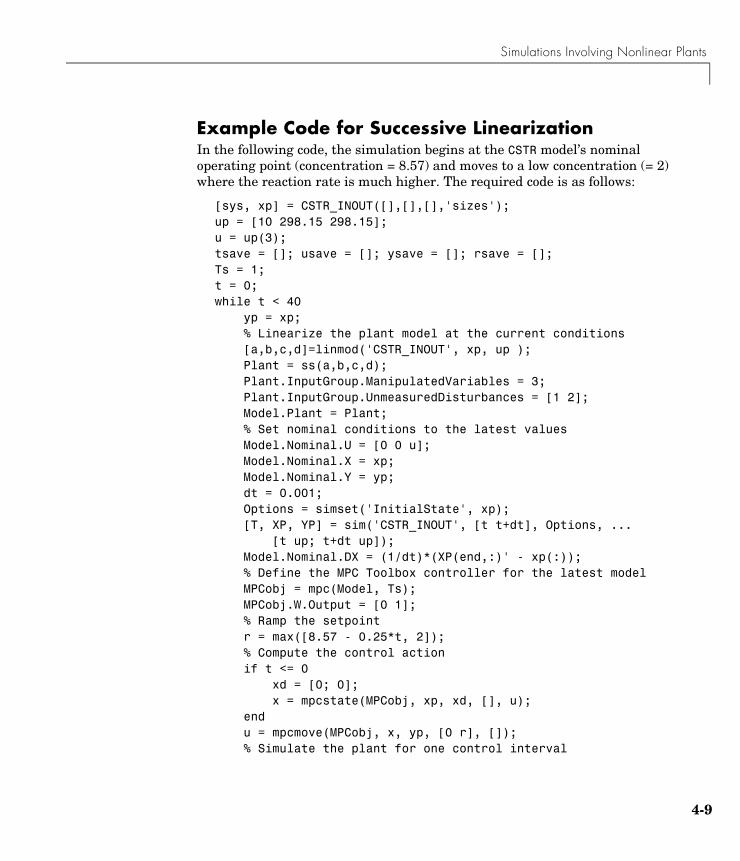
Simulations Involving Nonlinear Plants
4-9
Example Code for Successive LinearizationIn the following code, the simulation begins at the CSTR model’s nominal operating point (concentration = 8.57) and moves to a low concentration (= 2) where the reaction rate is much higher. The required code is as follows:
[sys, xp] = CSTR_INOUT([],[],[],'sizes');up = [10 298.15 298.15];u = up(3);tsave = []; usave = []; ysave = []; rsave = [];Ts = 1;t = 0;while t < 40 yp = xp; % Linearize the plant model at the current conditions [a,b,c,d]=linmod('CSTR_INOUT', xp, up ); Plant = ss(a,b,c,d); Plant.InputGroup.ManipulatedVariables = 3; Plant.InputGroup.UnmeasuredDisturbances = [1 2]; Model.Plant = Plant; % Set nominal conditions to the latest values Model.Nominal.U = [0 0 u]; Model.Nominal.X = xp; Model.Nominal.Y = yp; dt = 0.001; Options = simset('InitialState', xp); [T, XP, YP] = sim('CSTR_INOUT', [t t+dt], Options, ... [t up; t+dt up]); Model.Nominal.DX = (1/dt)*(XP(end,:)' - xp(:)); % Define the MPC Toolbox controller for the latest model MPCobj = mpc(Model, Ts); MPCobj.W.Output = [0 1]; % Ramp the setpoint r = max([8.57 - 0.25*t, 2]); % Compute the control action if t <= 0 xd = [0; 0]; x = mpcstate(MPCobj, xp, xd, [], u); end u = mpcmove(MPCobj, x, yp, [0 r], []); % Simulate the plant for one control interval

4 Using Model Predictive Control Toolbox Functions
4-10
up(3) = u; Options = simset('InitialState', xp); [T, XP, YP] = sim('CSTR_INOUT', [t t+Ts], Options, ... [t up; t+Ts up]); % Save results for plotting tsave = [tsave; T]; ysave = [ysave; YP]; usave = [usave; up(ones(length(T),1),:)]; rsave = [rsave; r(ones(length(T),1),:)]; xp = XP(end,:)'; t = t + Ts;endfigure(1)plot(tsave,[ysave(:,2) rsave])title('Residual Concentration')figure(2)plot(tsave,usave(:,3));title('Coolant Temperature')
CSTR Results and Discussion The plotted results appear below. Note the following points:
• The setpoint is being ramped from the initial concentration to the desired final value (see the step-wise changes in the reactor concentration plot below). The reactor concentration tracks this ramp smoothly with some delay (see the smooth curve), and settles at the final state with negligible overshoot. The controller works equally well (and achieves the final concentration more rapidly) for a step-wise setpoint change, but it makes radical changes in coolant temperature (not shown) that would probably be difficult to achieve in practice.
• The final steady state requires a coolant temperature of 305.20 K (see the coolant temperature plot below). An interesting feature of this nonlinear plant is that if one starts at the initial steady state (coolant temperature = 298.15 K), stepping the coolant temperature to 305.20 and holding will not achieve the desired final concentration of 2. In fact, under this simple strategy the reactor concentration stabilizes at a final value of 7.88, far from the desired value! A successful controller must increase the reactor temperature until the reaction “takes off,” after which it must reduce the
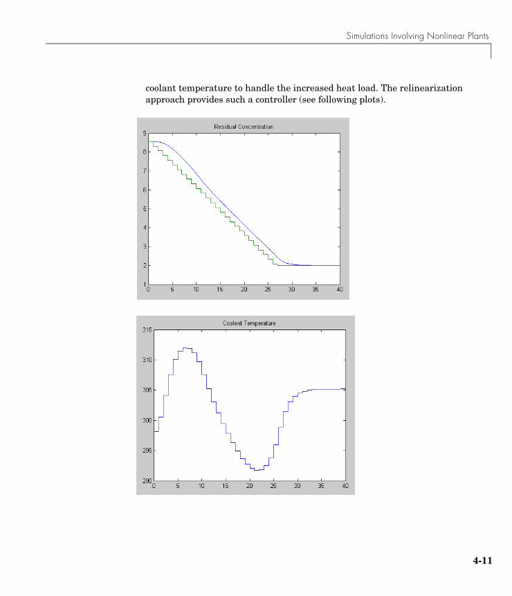
Simulations Involving Nonlinear Plants
4-11
coolant temperature to handle the increased heat load. The relinearization approach provides such a controller (see following plots).
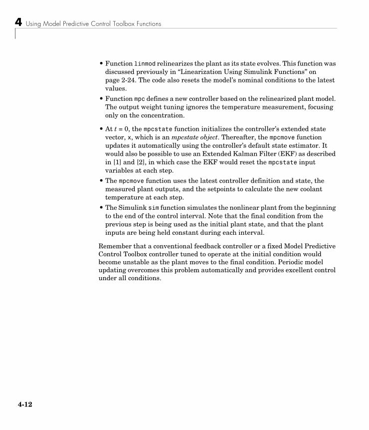
4 Using Model Predictive Control Toolbox Functions
4-12
• Function linmod relinearizes the plant as its state evolves. This function was discussed previously in “Linearization Using Simulink Functions” on page 2-24. The code also resets the model’s nominal conditions to the latest values.
• Function mpc defines a new controller based on the relinearized plant model. The output weight tuning ignores the temperature measurement, focusing only on the concentration.
• At t = 0, the mpcstate function initializes the controller’s extended state vector, x, which is an mpcstate object. Thereafter, the mpcmove function updates it automatically using the controller’s default state estimator. It would also be possible to use an Extended Kalman Filter (EKF) as described in [1] and [2], in which case the EKF would reset the mpcstate input variables at each step.
• The mpcmove function uses the latest controller definition and state, the measured plant outputs, and the setpoints to calculate the new coolant temperature at each step.
• The Simulink sim function simulates the nonlinear plant from the beginning to the end of the control interval. Note that the final condition from the previous step is being used as the initial plant state, and that the plant inputs are being held constant during each interval.
Remember that a conventional feedback controller or a fixed Model Predictive Control Toolbox controller tuned to operate at the initial condition would become unstable as the plant moves to the final condition. Periodic model updating overcomes this problem automatically and provides excellent control under all conditions.

Analysis Tools
4-13
Analysis ToolsThe are many ways to analyze a controller design. This section highlights two functions that support analysis of Model Predictive Control Toolbox controllers:
• “Steady-State Gain Computation” on page 4-13
• “Controller Extraction” on page 4-13
Steady-State Gain ComputationThe cloffset function computes the closed-loop, steady-state gain for each output when subjected to a sustained, 1-unit disturbance in each output. It assumes that no constraints will be encountered.
For example, consider the controller operating at the final steady-state of the nonlinear CSTR of the previous section. To compute its gain, type
cloffset(MPCobj)
which gives the result
ans =
1.0000 14.5910 -0.0000 -0.0000
The interpretation is that the controller doesn’t react to a sustained disturbance of 1 unit in the first output (the reactor temperature). Recall that this output has zero weight, so the controller ignores it. The same disturbance has no effect on the second output (the 2,1 element is zero).
If there is a 1-unit disturbance in the second output, the controller reacts, and the first output increases 14.59 units. The keeps the second output at its setpoint (the 2,2 element is zero).
Controller ExtractionUse the ss function to obtain an LTI representation of an unconstrained Model Predictive Control Toolbox controller. You can then use this to analyze closed-loop frequency response, etc.

4 Using Model Predictive Control Toolbox Functions
4-14
For example, consider the controller designed in “Creating a Controller Object” on page 4-2. To extract the controller, you could type
MPCss = ss(MPCobj);
You could then construct an LTI model of the closed-loop system using the feedback function (see the Control Systems Toolbox for details) by typing
CSTRd = c2d(CSTR, MPCss.Ts);CLsys = feedback(CSTRd, MPCss, 1, 2);
Note The CSTR model must be converted to discrete form with the same control interval as the controller.
You could then type
eig(CLsys)
to verify that all closed-loop poles are within the unit circle, or
bode(CLsys)
to compute a closed-loop bode plot, etc.

Bibliography
4-15
Bibliography[1] Lee, J.H. and N.L. Ricker, “Extended Kalman Filter Based Nonlinear Model Predictive Control,” Ind. Eng. Chem. Res., Vol. 33, No. 6,pp. 1530-1541(1994).
[2] Ricker, N. L., and J. H. Lee “Nonlinear Model Predictive Control of the Tennessee Eastman Challenge Process,” Computers & Chemical Engineering, Vol. 19, No. 9, pp. 961-981(1995)

4 Using Model Predictive Control Toolbox Functions
4-16

Index-1
Index
Bblocking 3-26
Ccloffset function 4-13closed-loop
design tool simulations 3-16constraints
input 3-29manipulated variable 3-29output 3-40softening 3-40
Control and Estimation Tools Manager 3-2control horizon
specification 3-19control interval
specification 3-19controller settings
blocking 3-26control interval 3-19delay compensation 3-48disturbance estimation 3-32get function 4-3horizons 3-19input constraints 3-29input weights 3-25move suppression 3-23output weights 3-22plant model 3-19prediction horizon 3-19rate weights 3-23set function 4-3weights 3-21
controllerscomparisons 3-26creation 4-2
design tool 3-19design tool list 3-8exporting 3-65LTI object extraction 4-13mpc function 4-2property settings 4-3robustness 3-44
CSTR (Continuous Stirred-Tank Reactor)linear model 2-5nonlinear model 2-20
Ddelays
controller settings for 3-48description
specification 3-5design tool
loading models 3-3starting 3-2tree navigation 3-7See also views
disturbance estimation 3-32disturbances
specification in simulations 3-16documentation 1-4
Eestimation
disturbances 3-32
Ggain
closed-loop 4-13
Index
Index-2
Hhorizons
specification 3-19
Iimport
plant model 3-4importing
controller 3-67InputGroup property 2-7InputName property 2-8inputs
manipulated variables 2-3measured disturbances 2-3names 2-8noise 2-16nominal value 3-5type specification 2-9types 2-3unmeasured disturbances 2-3
Llinearization
operating point 2-21repeated 4-9Simulink Control Design 2-19Simulink functions 2-24
linmod function 2-24loading
controllers 3-67project 3-67
LTI objectsproperties 2-7
Mmanipulated variables
definition 2-3measured disturbances
definition 2-3measured outputs
definition 2-3Model Predictive Control (MPC)
related products 1-5Toolbox 1-2
modelscharacteristics 2-13delays 3-47design tool list 3-8disturbances 3-32linearization 2-19loading into design tool 3-3LTI 2-4LTI chemical reactor 2-5noise inputs 2-16nonlinear 2-19nonlinear CSTR example 3-54nonlinear simulation 4-8nonsquare 3-52perturbation 3-44plant 2-2prediction error 3-44relinearizing 3-59Simulink 2-19state-space 2-5step response 2-17system identification 2-14transfer function 2-4zero/pole/gain 2-5See also system identification
MPC (Model Predictive Control)

Index
Index-3
See Model Predictive Controlmpc objects
conversion to state-space 4-13creating 4-2
mpcmove function 4-9mpcstate objects 4-10mpctool function
starting 3-2MV (manipulated variables)
See manipulated variables
Nnames
specification using design tool 3-5nominal values
specification 3-5nonlinear plants 3-54nonsquare plants 3-52
Oobjects
LTI 2-7mpc 4-2mpc conversion to ss 4-13mpcstate 4-10
open-loopdesign tool simulations 3-16
operating pointnew 2-21specification 2-21
OutputGroup property 2-7OutputName property 2-8outputs
measured 2-3names 2-8
nominal value 3-5setpoint definition 3-12type specification 2-9types 2-3unmeasured 2-3
Pplant/model mismatch 3-44plants
input/output signals 2-3MIMO 2-11nonlinear 3-54nonlinear simulation 4-8nonsquare 3-52
propertiesmpc object 4-3
Rresponse plots 3-14
data markers 3-14robustness
controller prediction error 3-44testing 3-44
Ssaving
controllers 3-65projects 3-66
scenariosdesign tool list 3-10specification 3-12
setpointsspecification 3-12
signal labels

Index
Index-4
description 3-5name 3-5units 3-5
signalsinputs 2-3outputs 2-3types 2-3
sim functionoptions 4-7simulations 4-6
simulationsclosed-loop 3-16conditions 3-12linear 3-12nonlinear 3-62open loop 3-16options 4-7sim function 4-6starting in design tool 3-14toolbar icon 3-13See also scenarios
soft constraints 3-40ss function 2-6state estimation 3-32SysID (System Identification)
See system identificationsystem identification
example 2-14model conversion 2-15noise inputs 2-16step response 2-17
Ttf function 2-4transfer functions
specification 2-4
treenavigation 3-7
typesspecification using design tool 3-5
Uunits
specification 3-5unmeasured outputs
definition 2-3
Vviews
constraint softening 3-41controller settings 3-19controllers 3-8plant models 3-8scenarios 3-10signal properties 3-7See also design tool
Wweights
inputs 3-25move suppression 3-23output 3-22rate 3-23setpoint tracking 3-22tuning 3-21
Zzpk function 2-5