Model Predictive Control Design for the Secondary ...

University of Wisconsin MilwaukeeUWM Digital Commons

Theses and Dissertations

May 2019

Model Predictive Control Design for theSecondary Frequency Control of MicrogridConsidering Time Delay AttacksZhengrong ChenUniversity of Wisconsin-Milwaukee

Follow this and additional works at: https://dc.uwm.edu/etdPart of the Electrical and Electronics Commons

This Thesis is brought to you for free and open access by UWM Digital Commons. It has been accepted for inclusion in Theses and Dissertations by anauthorized administrator of UWM Digital Commons. For more information, please contact [email protected].

Recommended CitationChen, Zhengrong, "Model Predictive Control Design for the Secondary Frequency Control of Microgrid Considering Time DelayAttacks" (2019). Theses and Dissertations. 2051.https://dc.uwm.edu/etd/2051

https://dc.uwm.edu/?utm_source=dc.uwm.edu%2Fetd%2F2051&utm_medium=PDF&utm_campaign=PDFCoverPages

https://dc.uwm.edu/etd?utm_source=dc.uwm.edu%2Fetd%2F2051&utm_medium=PDF&utm_campaign=PDFCoverPages

https://dc.uwm.edu/etd?utm_source=dc.uwm.edu%2Fetd%2F2051&utm_medium=PDF&utm_campaign=PDFCoverPages

http://network.bepress.com/hgg/discipline/270?utm_source=dc.uwm.edu%2Fetd%2F2051&utm_medium=PDF&utm_campaign=PDFCoverPages

https://dc.uwm.edu/etd/2051?utm_source=dc.uwm.edu%2Fetd%2F2051&utm_medium=PDF&utm_campaign=PDFCoverPages

mailto:[email protected]

MODEL PREDICTIVE CONTROL DESIGN FOR THE SECONDARY FREQUENCY

CONTROL OF MICROGRID CONSIDERING TIME DELAY ATTACKS

by

Zhengrong Chen

A Thesis Submitted in

Partial Fulfillment of the

Requirements for the Degree of

Master of Science

in Engineering

at

The University of Wisconsin-Milwaukee

May 2019

ii

ABSTRACT

MODIFIED MODEL PREDICTIVE CONTROL STRATEGY FOR MICROGRID SECONDARY FREQUENCY CONTROL WITH TIME DELAY ATTACKS

by

Zhengrong Chen

The University of Wisconsin-Milwaukee, 2019 Under the Supervision of Professor Lingfeng Wang

Fast depleting fossil fuels and growing awareness of environmental protection have

raised worldwide concerns, aiming to build a sustainable and smart energy ecosystem.

Renewable energy generation plays an important role in providing clean power supply.

However, the integration of a bulk renewable generation system would also introduce new

forms of disturbances and uncertainties to impact the power quality, threatening the secure

operation of the distribution network. Microgrid, as an emerging technology, is quite

appealing to be interfaced with distribution systems due to its potential economic,

environmental, and technical benefits. The microgrid differs from the “smart grid” with

different control strategies to accomplish the goal of helping the power grid with load

balancing and voltage control and assisting power markets. A hierarchical control structure

for the microgrid is commonly designed to address all above issues both in islanded mode

and grid-connected mode.

On the other hand, concerns about cybersecurity threats in the microgrid are steadily

iii

rising, and enormous number of economic losses would occur if defense strategies are not

stipulated and carried out. In the modern power system, distributed control system, intelligent

measuring devices and Internet of Things (IoT) are highly recommended in microgrid

systems, which lead to the vulnerability of communication channels. Cyber threats such as

false data injection (FDI) attacks, denial of service (DoS) attacks, and time-delay switch

attacks (TDS) can be effortlessly implemented through information and communication

centers, compromising the secure operation of power systems. By theoretically analyzing the

AC microgrid simulation model, the MPC control strategies, and the modified MPC method

based on GCC estimation will be studied in this thesis.

In the second chapter, this thesis summarizes the start-art-of microgrid control,

introducing a hierarchical control structure: primary control, secondary control, and tertiary

control. These control levels differ in their speed of response, the time frame in which they

operate, and infrastructure requirements. We focus on the centralized secondary frequency

control system, which compensates the frequency deviation caused by primary control—P/f

method.

Then, in Chapter 3, the isolated AC MG frequency control system including WTG,

DEG, PV panel and energy storage system with MPC controller is modeled. Three case

studies are designed in MATLAB/Simulink to illustrate the advantages of the MPC method

compared with the traditional PI controller.

In the next Chapter, since state estimation based on precise status feedback of the system

components is essential for the MPC controller to calculate corresponding control signal, the

status feedback attack to BESS and FESS is considered. Correspondingly, an online status

iv

switching method is proposed to detect the original statuses of BESS and FESS, updating the

state estimation function to obtain desirable performance of frequency regulation.

Last, considering the time delay attack hacked by the adversary in the sensor, a modified

MPC method based on GCC estimation is proposed to detect and track time delay attacks

online. The model of proposed method to regulate frequency deviation is built in MATLAB.

There are three case studies in this part: a constant time-delay attack with 0.1 pu load

increase; a time-varying delay attack with 0.1 pu load increase; and a time-varying delay

attack with changing load disturbance. By analyzing results of three cases, the effectiveness

of the modified MPC method is proved.

v

© Copyright by Zhengrong Chen, 2019

All Rights Reserved

vi

TABLE OF CONTENTS ABSTRACT ............................................................................................................................................... ii

LIST OF FIGURES .................................................................................................................................. viii

LIST OF TABLES ....................................................................................................................................... x

LIST OF ABBREVIATIONS ........................................................................................................................ xi

ACKNOWLEDGMENTS ........................................................................................................................... xii

Chapter 1：Introduction ....................................................................................................................... 1

1.1 MG: background and motivation ................................................................................................. 1

1.2 MG: cyber-attack risk ................................................................................................................... 3

1.3 Research objectives ..................................................................................................................... 5

1.4 Thesis contribution ...................................................................................................................... 6

Chapter 2：MG control state-of-the-art ............................................................................................... 8

2.1 Hierarchical structure .................................................................................................................. 8

2.2 Primary control ............................................................................................................................ 9

2.2.1 Inverter output control ....................................................................................................... 10

2.2.2 Power sharing control ......................................................................................................... 11

2.3 Secondary control ...................................................................................................................... 13

2.3.1 Centralized frequency control ............................................................................................ 13

2.3.2 Distributed frequency control ............................................................................................ 15

Chapter 3：MG frequency control: modelling .................................................................................... 17

3.1 Configuration of an islanded microgrid ..................................................................................... 17

3.1.1 Modelling of frequency response ....................................................................................... 17

3.1.2 Characteristics of output power of WTG and PV ................................................................ 19

3.1.3 The transfer functions of various generation subsystems .................................................. 20

3.1.4 Transfer functions of different energy storage systems ..................................................... 20

3.1.5 System frequency variation ................................................................................................ 21

3.2 Conventional PI controller ......................................................................................................... 21

3.2.1 Frequency control model .................................................................................................... 21

3.2.2 WTG model and PV model .................................................................................................. 23

3.2.3 Simulation in Simulink ........................................................................................................ 24

3.3 Model predictive control ........................................................................................................... 27

vii

3.3.1 Principle of MPC ................................................................................................................. 27

3.3.2 MPC controller for MG frequency control .......................................................................... 28

3.4 Case study .................................................................................................................................. 31

3.4.1 Case design ......................................................................................................................... 31

3.4.2 Simulation result and discussion ........................................................................................ 32

Chapter 4: MPC status feedback attack ............................................................................................... 38

4.1 Attack description ...................................................................................................................... 38

4.2 Online switching method ............................................................................................................... 40

4.3 Case study ...................................................................................................................................... 41

Chapter 5: Modified MPC controller under time-delay attack ............................................................ 44

5.1 Time delay attack ....................................................................................................................... 44

5.2 MPC controller under time-delay attack ................................................................................... 46

5.2.1 Modelling ............................................................................................................................ 46

5.2.2 Case study with known time-delay signal ........................................................................... 47

5.3 Modified MPC with online time-delay estimation ..................................................................... 50

5.3.1 Methodology ...................................................................................................................... 50

5.3.2 Generalized cross correlation ............................................................................................. 51

5.3.3 Algorithm of controller design ............................................................................................ 52

Chapter 6: Case study .......................................................................................................................... 54

6.1 Modified MPC model simulation ............................................................................................... 54

6.1.1 Case 1: constant time-delay attack ..................................................................................... 54

6.1.2 Case 2: time-varying delay attack ....................................................................................... 56

6.1.3 Case 3: two steps load disturbance .................................................................................... 57

6.2 Discussion .................................................................................................................................. 59

Chapter 7: Conclusion and future work ............................................................................................... 60

7.1 Conclusion ................................................................................................................................. 60

7.2 Future work ............................................................................................................................... 61

REFERENCES ......................................................................................................................................... 63

viii

LIST OF FIGURES

Figure 1.1 Attacks on control loop ......................................................................................................... 4

Figure 2.1 Hierarchical control levels of microgrid ............................................................................... 8

Figure 2.2 Current and voltage control loops ...................................................................................... 10

Figure 2.3 P-f droop curve ................................................................................................................... 12

Figure 2.4 Q-V droop curve ................................................................................................................. 12

Figure 2.5 Centralized secondary control system for frequency regulation ......................................... 14

Figure 2.6 Distributed secondary control system for frequency regulation ......................................... 16

Figure 3.1 Single-line diagram of the ac MG ...................................................................................... 18

Figure 3.2 Conventional PI Frequency response model for the ac MG system ................................... 22

Figure 3.3 Wind turbine output ............................................................................................................ 23

Figure 3.4 Solar radiation and PV output power .......................................................................... 24

Figure 3.5 Simulink scheme-PI ........................................................................................................... 25

Figure 3.6 (a) Multiple step load disturbances (b) MG frequency response ........................................ 26

Figure 3.7 Frequency control following a step load disturbance of 0.1 pu .......................................... 26

Figure 3.8 MPC framework ................................................................................................................. 28

Figure 3.9 Simulink scheme-MPC ....................................................................................................... 30

Figure 3.10 Case1 control system scheme ........................................................................................... 32

Figure 3.11 Frequency control following a step load disturbance of 0.1 p.u ....................................... 33


Figure 3.13 Frequency control following a step load disturbance of 0.1 p.u ....................................... 35


F

ix

Figure 3.15 Case 3 frequency control following a step load disturbance of 0.1 p.u ............................ 36

Figure 3.16 Comparison for three cases .............................................................................................. 36

Figure 4.1 Scheme of MPC status feedback attack .............................................................................. 39

Figure 4.2 Status feedback attack online detection block .................................................................... 40

Figure 4.3 Frequency response under status feedback attack .............................................................. 42

Figure 4.4 Frequency response with online switching method under status feedback attack .............. 43

Figure 4.5 Online detection of statues of BESS and FESS .................................................................. 43

Figure 5.1 A simplified load frequency control system under time-delay attack ................................. 45

Figure 5.2 Dynamic model of MPC frequency control with delay attack ............................................ 46

Figure 5.3 MPC control block diagram under attack ........................................................................... 46

Figure 5.4 Frequency respond when =0.1s ...................................................................................... 48




Figure 5.8 Block diagram of proposed control technique .................................................................... 50

Figure 6.1 GCC delay estimation in case1 ........................................................................................... 55

Figure 6.2 Frequency response following a step load disturbance of 0.1 pu ....................................... 55

Figure 6.3 (a) Frequency output of microgrid system in case 2 (b) time-varying delay estimation ..... 56

Figure 6.4 Two steps load disturbance ................................................................................................. 57

Figure 6.5 GCC time delay estimation in case 3 .................................................................................. 58

Figure 6.6 Frequency response in case 3 ............................................................................................. 58

t

t

t

t

x

LIST OF TABLES

TABLE I RATED POWER OF DG UNITS AND LOADS ................................................................. 18

TABLE II THE PARAMETERS VALUES OF THE AC MG SYSTEM ............................................ 23

TABLE III CASE STUDY DESIGN ................................................................................................... 32

xi

LIST OF ABBREVIATIONS

MG Microgrid MPC Model predictive control IoT Internet of things FDI False data injection DoS Denial of service TDS Time-delay switch GCC Generalized cross correlation WTG Wind turbine generation DEG Diesel engine generation PV Photovoltaics BESS Battery energy storage system FESS Flywheel energy storage system FC Fuel cell PI Proportional–integral RES Renewable energy source DER Distributed Energy Resources DGRs Distributed generation resources DG Distributed generators CHP Combined heat and power LV Low voltage MV Medium voltage DSM Demand side management PCC Point of common coupling ICT Information & communication technology PMU Phasor measurement units LFC Load frequency control LMIs Linear matrix inequalities RMSE Root-mean-square error VSIs Voltage-Source Inverters VSC Voltage-Source Converter PLL Phase locked loop SISO Single-input single-output MIMO Multi-input multi-output SCS Secondary control system

xii

ACKNOWLEDGMENTS

I cannot express enough thanks to my advisor, Prof. Lingfeng Wang, for his constructive

guidance in the cutting-edge research on reliability and cybersecurity of power systems and

also for his kindness and support in my daily life and study. Moreover, I would like to thank

Dr. Zhaoxi Liu who helped me develop the model and case studies of this thesis.

Secondly, I would like to express my sincere gratitude to the committee members, Prof.

Yi Hu and Prof. Zeyun Yu for their insightful and valuable comments.

I also want to give enormous thanks to my labmates in the Laboratory of Trustworthy

Cyber-Physical Systems and Infrastructures for your help and support.

I am also grateful for the financial support for me to perform the research of this thesis.

This work was supported in part by the National Science Foundation under Award

ECCS1711617, in part by the Research Growth Initiative Program of University of Wisconsin-

Milwaukee under Award 101X360, and in part by the National Science Foundation

Industry/University Cooperative Research Center on Grid-connected Advanced Power

Electronic Systems (GRAPES) under Award GR-18-06.

Finally, I am grateful for the continued support and encouragement from my parents,

family, and friends throughout my graduate education.

1

Chapter 1：Introduction

1.1 MG: background and motivation

With the development of electrical industry, bulk power systems and reliable supply of

energy are highly emphasized. Growing concerns for the primary energy structure and aging

infrastructure of current electrical transmission and distribution networks are increasingly

challenging security, reliability and quality of power supply. According to the International

energy agency [1], energy demand is set to grow by more than 25% to 2040, requiring more

than $2 trillion a year of investment in new energy supply. Thus, renewable energy sources

(RESs) are mostly appealing one which can be used as alternative generation units in the

modern power system to meet the need of efficient energy supply and low carbon economy.

The increasing penetration of the RESs has many advantages, but also introduces new

challenges as whether those sources can operate stable beside conventional generation units or

not.

It is worth noting that the power systems have always been “smart”, especially at the

transmission level. However, the distribution level need to be transformed from passive to

active networks, especially in the sense that control is distributed and power flows are

bidirectional. Power generation can be linked to the customers load, taking all kinds of

information to get the best operation point to reduce the total cost in real time.

The microgrid concept is a quite appealing to address above problems, specifically in the

field of integrating Distributed Energy Resources (DER) into power system, as well as

2

distributed energy-storage systems. It consists of Distributed generators (DG, e.g. diesel

engines, Micro Turbines, PV, wind turbines and CHP), storage units, Renewable energy

Resources and loads [2-4]. Commonly, the energy-storage systems include pumped storage,

compressed air energy storage, batteries, ultra-capacitors, flywheels, plug-in hybrid electric

vehicles, etc. From a grid point of view, microgrids can be viewed as control entities within the

power system. From the customer's point of view, microgrids and traditional low-voltage

distribution networks provide heat and power requirements [5].

The MGs are mostly placed in the low voltage (LV) and medium voltage (MV)

distribution networks [6]. With numerous micro-sources connected at the distribution level,

there are new challenges, such as system stability, power quality, and network operation that

must be resolved applying the advanced control techniques at LV/MV levels rather than high

voltage levels which is common in conventional power system control.

The difference between microgrid and smart grid mainly depends on their control structure.

So proper and complicated control is required for microgrid through which we can facilitate

the effective integration of DER and ensure the operation to be stable and economically

efficient. The principal roles of the microgrid control structure are [2]:

l Voltage and frequency regulation for both operating modes and seamless transition

between two modes

l Proper load sharing and DER coordination

l Power flow control between the microgrid and the main grid

l Schedule and dispatch of units under supply and demand uncertainty

l Optimizing the microgrid operating cost

3

l Design of appropriate DSM schemes to allow customers to react to the grid’s need

Microgrid can operate in both grid-connected and islanded operating modes to avoid huge

loss caused by external faults [7]. In the grid-connected mode, active and reactive power can

be shared through point of common coupling (PCC) connected to the main grid. So in the

steady state, the system state e.g. voltage and frequency are necessarily following the nominal

values. But in the islanded mode, the control issue becomes more difficult and intricate because

of dynamic fluctuation and loss of communication with nominal points. More detailed control

structure and advance control algorithm are required for the islanded mode to achieve voltage,

current and frequency regulation in the MG.

1.2 MG: cyber-attack risk

Microgrid takes advantages of advanced control strategies, cost-competitive technologies

and information & communication technology (ICT). In order to achieve stable and efficient

operation of power system and DER units locally controlled, it’s necessary to expend cyber

network inter-connectivity so that information may flow freely and correctly. But, in the

meanwhile, the communication channel and controller in power system will become more

vulnerable to cyber threats. A campaign of cyberattacks disabled safety systems at the Davis-

Besse nuclear power plant in 2003 [8]. In 2004, the U.S. Department of Energy (DOE)

estimated the cost of the blackout is approximately $6 billion on cybersecurity threats in

computer-based systems [9]. This large-scale blackout was caused by a software failure in the

IT system, which shows that a deliberate attack would be much more catastrophic. In 2010, the

Stuxnet norm was discovered, which was designed to target proprietary (Siemens) SCADA

systems in an Iranian power plant. In 2015, the Ukrainian power grid was attacked by the cyber

4

attackers, which was considered the first cyber-attack event causing power blackouts [11].

Cyber attacks mainly include DoS attacks, false data injection attacks (FDI), malware,

time-delay attacks and virus attacks. A DoS attack is a resource-exhausting attach that makes

the server or communication network cannot provide normal services by sending a lot of

useless command [12]. FDI attacks exploit the sensor (e.g. phasor measurement units, PMU)

measurements by injecting false information, maliciously destroying the system performance.

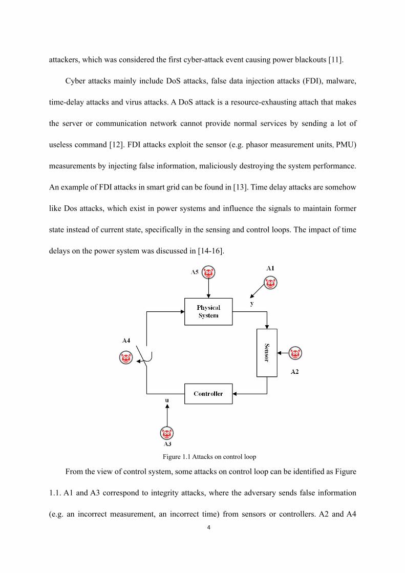
An example of FDI attacks in smart grid can be found in [13]. Time delay attacks are somehow

like Dos attacks, which exist in power systems and influence the signals to maintain former

state instead of current state, specifically in the sensing and control loops. The impact of time

delays on the power system was discussed in [14-16].

Figure 1.1 Attacks on control loop

From the view of control system, some attacks on control loop can be identified as Figure

1.1. A1 and A3 correspond to integrity attacks, where the adversary sends false information

(e.g. an incorrect measurement, an incorrect time) from sensors or controllers. A2 and A4

5

correspond to DoS attacks and time-delay attacks. The adversary will prevent the controller

from receiving correct sensor measurements or prevents actuators from receiving control

commands. The attackers can launch a DoS attack or time-delay attacks by jamming

communication channels, compromising devices and preventing them from sending data,

attacking routing protocols, or flooding the network. Finally, A5 corresponds to a direct attack

against actuators or an external physical attack on the plant [17].

Several studies have assessed the time delay attacks and their impact on the stability of

power system. Reference [18] use phasor measurements with delays to design a two-level

control structure, and small signal stability of the power system was considered. In [19], a

delay-dependent robust method is proposed for analysis of a PID-type LFC scheme considering

time delays. The time-delay estimator based on gradient descent method and a modified least

mean square minimization technique was proposed in [20]. Authors in [22] take Lyaponuv-

theory and linear matrix inequalities (LMIs) techniques to analyze the delay time bound of

stable LFC scheme. However, there are few control methods that perform online estimation of

dynamic time delays and real-time control of power systems. Furthermore, few studies

considered the control of power systems with time delays introduced by adversary.

1.3 Research objectives

The control system is the key part of the microgrid with the goal to solve the power

dispatch issue, decrease the loss of the transmission line and improve the reliability of electric

power system. In the traditional microgrid control system, the close-loop controllers based on

proportional-integral-derivative (PID) are widely utilized. However, due to the complex multi-

objective regulation problems in modern MG systems and uncertainty caused by RES,

6

traditional PID controllers are unable to provide a proper performance. The MPC controllers

can be much more powerful and flexible. Besides, MPC can effectively overcome the

uncertainty and non-linearity of the process, and deal with the variables constraints in

processing manipulated variables [22].

The present thesis focuses on the MG frequency regulation, as a secondary control issue.

There are three following objectives:

1) Model the MG frequency control system in isolated mode

2) Apply MPC controller as a secondary control part

3) Consider the status feedback attack to FESS and BESS system

4) Prevent the impact of time-delay attack in the control system

1.4 Thesis contribution

This thesis work has been guided by the purpose to realize frequency control in MG and

maintain a generation-load balance. Moreover, stability of MG frequency control system is

evaluated when considering time-delay attack in the communication channel. Then, some

adjustments must have to be applied to eliminate the instability and devastation caused by

adversary.

The contribution in this thesis will be as following:

l Modeling the isolated ac MG system including WTG, DEG, PV panel and energy

storage system.

l Realizing the MPC controller to control the frequency in the microgrid simulation in

MATLAB/Simulink and comparing MPC method with the traditional PI controller to

introduce its advantages.

7

l Creating an online switching method which takes RMSE to identify the real statuses

of BESS and FESS when considering the status feedback attack to the state estimation

of MPC controller.

l Proposing a modified MPC control algorithm based on a GCC time-delay estimation

to obtain stable frequency regulation in real time, when considering constant or time-

varying delay attack.

8

Chapter 2：MG control state-of-the-art

2.1 Hierarchical structure

With the regard to the principal roles of the microgrid control scheme, a hierarchical

control structure is required to address different significances and time scales among microgrid

control demand. Hierarchical control strategy consists of three levels, namely the primary,

secondary, and tertiary controls, as shown in Figure 2.1. These control levels differ in their (i)

speed of response and the time frame in which they operate, and (ii) infrastructure requirements

(e.g., communication requirements) [22,23].

Figure 2.1 Hierarchical control levels of microgrid

The primary control, known as local control, maintains voltage and frequency stability of

the microgrid. Based on local measurements, islanding detection, output control and power

9

sharing (and balance) control are included in this category. It is essential to provide independent

active and reactive power sharing controls for the DERs in the presence of both linear and

nonlinear loads. Thus, Voltage-Source Inverters (VSIs) are used as interface for DC sources.

Meanwhile, inverter output controllers should control and regulate the output voltages and

currents to satisfy power sharing control. The secondary control is responsible for the reliable,

secure and economical operation of microgrids in either grid-connected or stand-alone mode,

compensating for the voltage and frequency deviations caused by the operation of the primary

controls. Ultimately, the tertiary control is the highest level of control and manages the optimal

operation of all microgrids interacted. This control level provides signals to secondary level

controls at microgrids and other subsystems that form the full grid. Tertiary control can be

regarded as part of the host grid, and some parts beyond the microgrid. Therefore, this control

level is not discussed in this thesis.

2.2 Primary control

The primary control is designed to address the following tasks:

l To stabilize voltage and frequency due to the mismatch between the power generated

and consumed.

l To offer plug and play capability for DERs and properly share the active and reactive

power among them.

l To regulate the currents to protect power electronic devices and the DC-link capacitor.

As more RES are commonly used in modern power system to improve energy structure,

voltage-source inverters (VSIs) are required as interface for DC sources (e.g. solar power and

wind power). VSI controllers are composed of two stages: inverter output controller and DG

10

power sharing controller.

2.2.1 Inverter output control

The inverter output control typically consists of an outer loop for voltage control, and an

inner loop for current regulation. These inner control loops are commonly referred to as zero-

level control, which have fast response speed and can keep the manipulated variables tracking

the references [24].

The primary control will provide the reference points for the voltage and current control

loops of DERs [25]. The nested voltage and frequency control loops are shown in Figure 2.2.

The error signal, obtained by sensed signal from AC bus and reference signal, will be processed

by voltage controller to compute the corresponding control signal. And inner current control

loop, conventionally with additional feed-forward current compensation to regulate the current

of VSC output.

Figure 3.2 Current and voltage control loops

In general, PI controllers are commonly used in above control loops, obtaining content

performance of voltage and current regulation. Besides, multivariable control methods have

been proposed in [26], [27] to improve the dynamic response of microgrids and ensure robust

11

stability against uncertainties in load parameters due to presence of nonlinear loads.

2.2.2 Power sharing control

The usual method to accomplish active and reactive power sharing is to use Q-V and P-f

droop control algorithms [22,23,28]. When two points in the network are operating at different

frequencies there is an increase of active power delivery from the location of higher frequency

to the location of lower frequency. As this happens, the two frequencies tend to drift towards a

common average value until the new steady state is reached (self-synchronizing torque). If the

network exists mismatch for reactive power, the situation can be solved by regulating voltage

in the system.

When considering different configuration of converters, there are several methods to

address active and reactive power control such as centralized [29], master-slave [30],

decentralized [31] and droop [32]. Due to space limitation, this thesis mainly presents 2.2.3

Droop control method.

In droop control, the relationship between real power/frequency and reactive

power/voltage can be expressed as [25]:

(2.1)

where and are the DER output voltage RMS value and nominal frequency,

respectively. The droop coefficients, and , can be adjusted either heuristically or by

tuning algorithms.

By linearizing it, frequency droop characteristic is

(2.2)

0 p

Q

D PV V D Qw w*

*

ì = -ïí = -ïî

V * w*

pD QD

0 pD Pw w*D = D - D

12

The droop characteristic curve is shown in Figure 2.3 and Figure 2.4.

Figure 4.3 P-f droop curve

Figure 5.4 Q-V droop curve

The advantages of droop control are that it can be implemented with no communication

links and the control action is merely based on local information. Those features make droop

control more flexible and reliable than other methods. Some works address the scheduling of

13

the droop coefficients for frequency regulation in the MGs [33]. As described in [34], [35],

frequency stability in a power system means preserving steady frequency following a heavy

disturbance with minimum loss in loads and generation units.

However, in the steady state, the system will settle down to a new operating point where

the MG frequency and voltage are not equal to the nominal value. Therefore, in some studies,

a secondary control which compensate the voltage and frequency deviations caused by the

droop control is required to be designed.

2.3 Secondary control

As mentioned, secondary control is responsible for the secure, economical and reliable

operation of the microgrid. When in the steady state, secondary control will restore the

microgrid voltage and frequency, compensating the deviations caused by the primary control.

This control hierarchy will have slower dynamic response than that of the primary, which

reduces the harmonic content of the voltage waveform.

There are two topologies for secondary control: centralized and distributed. While the

centralized topology proposes a central controller to make decisions, the distributed topology

allows the interaction of various units within the microgrid and realization of self-control. It’s

obvious that the distributed approach can exhibit the desirable plug-and-play feature, which

may be the trend of microgrid control topology.

This thesis focuses on frequency regulation of the microgrid. A related detailed description

of the centralized and decentralized approaches is presented next.

2.3.1 Centralized frequency control

14

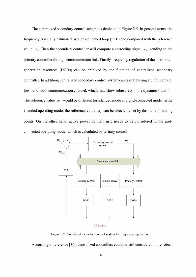
The centralized secondary control scheme is depicted in Figure 2.5. In general terms, the

frequency is usually estimated by a phase locked loop (PLL) and compared with the reference

value . Then the secondary controller will compute a correcting signal sending to the

primary controller through communication link. Finally, frequency regulation of the distributed

generation resources (DGRs) can be archived by the function of centralized secondary

controller. In addition, centralized secondary control system can operate using a unidirectional

low bandwidth communication channel, which may show robustness in the dynamic situation.

The reference value would be different for islanded mode and grid-connected mode. In the

islanded operating mode, the reference value can be directedly set by desirable operating

points. On the other hand, active power of main grid needs to be considered in the grid-

connected operating mode, which is calculated by tertiary control.

Figure 6.5 Centralized secondary control system for frequency regulation

According to reference [36], centralized controllers could be still considered more robust

nw sw

nw

nw

15

and reliable than distributed one in MGs located in developing countries and/or rural areas

where good communication infrastructure is not always available. However, huge losses may

occur due to a system collapse if failure happens to the communication channel. Hence, it’s

essential to discuss the security and stability of MG secondary control.

2.3.2 Distributed frequency control

The distributed control framework, in comparison of the centralized control strategy, uses

the recent advances in communication technologies, such as WiFi and Zigbee technologies,

and also new algorithms for exchange of information (such as gossip, consensus, OpenFMB)

[37]. A typical distributed secondary control is shown as Figure 2.6. In this case, each

generation unit is provided with secondary control capacity to correct the frequency deviation.

Moreover, each DGR is equipped with PLLs to estimate voltage and frequency at PCC. In some

area, the distributed secondary control system looks promising because of its autonomous

capacity for each DGR. But the use of high the high-bandwidth required by distributed

secondary control could compromise the MG robustness.

16

Figure 7.6 Distributed secondary control system for frequency regulation

Some efforts have been taken to mitigate the effect of communication link failures.

Authors in [38] present a secondary control with no communications for islanded microgrids,

where switches between two configurations according to a time-dependent protocol exist to

archive frequency restoration. Event-trigger based secondary control methods are new

approaches to reduce the communication band-width in [39]. Moreover, state estimation based

secondary control strategy has been introduced to control voltage in MG [40].

17

Chapter 3：MG frequency control: modelling

3.1 Configuration of an islanded microgrid

3.1.1 Modelling of frequency response

Combing the renewable energy resource (e.g. solar power, wind power, water energy) with

different energy storage systems in microgrid system, the generated electric power can meet

the requirement of connected loads. Taking the model of the isolated MG system in thesis [41],

which is shown in Figure 3.1. The MG system contains conventional diesel engine generator

(DEG), PV panel, wind turbine generator (WTG), fuel cell (FC) system, battery energy storage

system (BESS), and flywheel energy storage system (FESS). As shown in Figure 3.1, the DGs

are connected to the MG by power electronic interfaces which are used for synchronization in

ac sources like DEG and WTG and to reverse voltage in dc sources like PV panel, FC, and

energy storage devices. The FC contains three fuel blocks, an inverter for converting dc to ac

voltage and an interconnection device (IC). The FC has a high-order characteristic but a three-

order model is sufficient for frequency studies [42]. Both FC and DEG are considered as parts

of frequency secondary control to reduce the deviation.

18

Figure 8.1 Single-line diagram of the ac MG

The circuit breaker is used in each microsource to disconnect from the network to avoid

the impacts of severe disturbances through the MG or for maintaining purposes. Nominal

values of the DG units and loads are given in TABLE I.

TABLE I RATED POWER OF DG UNITS AND LOADS

Rated power (KW) Load (KW)

WTG 100

210 PV panel 30

FC 70

DEG 160

210 FESS 45

BESS 45

1LP

2LP

19

The power balance function can be described as:

(3.1)

where, the exchange power of FESS and BESS may be bilateral. FC and DEG are standby

generators that deliver power to the system only when the total power generated by the WTG

and PV is insufficient.

To precisely simulate the dynamic behaviors of practical WTG, DEG, FC, BESS, FESS,

PV, etc., physical system must be extracted into mathematical model. For large-scale power

system, however, simplified models or transfer functions are generally employed.

3.1.2 Characteristics of output power of WTG and PV

The output power of the studied wind turbine is determined by nondimensional curves of

power coefficient , which is a function of tip speed ratio and blade pitch angle . The

tip speed ratio can be defined by

(3.2)

where (=23.5m) is the radius of blades and (=3.14 rad/s) is the rotational

speed of blades. The function of is given by

(3.3)

The output mechanical power of the mentioned WTG is

(3.4)

where (=1.25 ) is the air density. is the swept area of blades, which is 1735 .

is the wind speed.

The output power of the studied PV system is characterized by

LOAD L1 L2 WTG PV FC DEG FESS BESSP P P P P P P P P= + = + + + ± ±

pC l b

blade blade

W

RVwl =

bladeR bladew

pC

( 3)(0.44 0.0167 )sin 0.0184( 3)15 0.3pCp lb l b

bé ù-

= - - -ê ú-ë û

312W r p WP AC Vr=

r 3kg/m rA2m

WV

20

(3.5)

where is the conversion efficiency of the PV arrays, commonly ranging from 9% to

12%. S is the measured area of the PV array, is the solar radiation and is ambient

temperature in degree Celsius. In this thesis, S=4084 and is kept at 25 . Therefore,

is linearly varied with only.

3.1.3 The transfer functions of various generation subsystems

The transfer functions of the WTG, PV, FC, and DEG shown in Figure 3.1 are, respectively,

represented as given:

(3.6)

(3.7)

(3.8)

(3.9)

3.1.4 Transfer functions of different energy storage systems

Energy storage systems are essential to support insufficient energy of power generation

subsystems of the microgrid system within a very short time to maintain system stability.

Because the BESS takes time to charge energy to the battery cells or release the energy from

the battery, its time constant is limited to several seconds. On the other hand, the FESS can

store surplus energy during off-peak periods and quickly release energy during peak loads. The

transfer functions of the BESS and FESS can be, respectively, expressed as a first-order lag as

given next:

{ }1 0.005( 25)PV aP S Th= F - +

h

F aT

2m aT C°

PVP F

( ) WTG WTGWTG

WTG W

K PG s1 sT P

D= =

+ D

( ) PV PVPV

PV

K PG s1 sT

D= =

+ DF

/

( ) FC FCFC

FC IN I C

K P1 1G s1 sT 1 sT 1 sT f

D= × × =

+ + + D

( ) DEG DEGDEG

DEG t

K P1G s1 sT 1 sT f

D= × =

+ + D

21

(3.10)

(3.11)

3.1.5 System frequency variation

In the autonomous microgrid system, the total power generation must meet the total power

demand of the connected loads to maintain the stable operation. However, due to the difference

between power demand reference and total power generation , the system

frequency would wave. Hence, P-f control method mentioned in Chapter 2 is required to track

the reference frequency.

(3.12)

The system frequency variation is calculated by

(3.13)

where is system frequency characteristic constant of the microgrid system. The

transfer function for system frequency variation to per unit power deviation can be expressed

by

(3.14)

where D and M are, respectively, the equivalent inertia constant and damping constant

[43].

3.2 Conventional PI controller

3.2.1 Frequency control model

( ) BESS BESSBESS

BESS

K PG s1 sT f

D= =

+ D

( ) FESS FESSFESS

FESS

K PG s1 sT f

D= =

+ D

ePD dP*

gP

e d gP P P*D = -

fD

e

sys

PfKD

D =

sysK

( )( )sys

e sys sys

f 1 1G sP K 1 sT D sMD

= = =D + +

22

Figure 9.2 Conventional PI Frequency response model for the ac MG system

After modelling the microgrid frequency control system by transfer functions, a simplified

frequency response model is shown in Figure 3.2. Parameter values of the block diagram of all

following cases are given in TABLE II. Conventional frequency response model for the ac MG

system is discussed where PI controller is responsible for the secondary control to compensate

frequency deviation.

23

TABLE II THE PARAMETERS VALUES OF THE AC MG SYSTEM

Parameter Value Parameter Value

D 0.015 0.08

2H 0.1667 0.4

0.1 0.004

0.1 0.04

0.26 R 3

1 1.8

1 1.5

3.2.2 WTG model and PV model

In this thesis, the total power of the connected loads for all simulation case study is

assumed to be 1.0 pu under normal operating condition. And is set to be 7.5 m/s and

is kept to be a smooth curve less than 0.3 pu. According to former assumptions, output of WTG

and output of PV are depicted in Figure 3.3 and Figure 3.4.

Figure 10.3 Wind turbine output

gT

tT

FESST CT

BESST INT

FCT

PVK PVT

WTGK WTGT

WV F

24

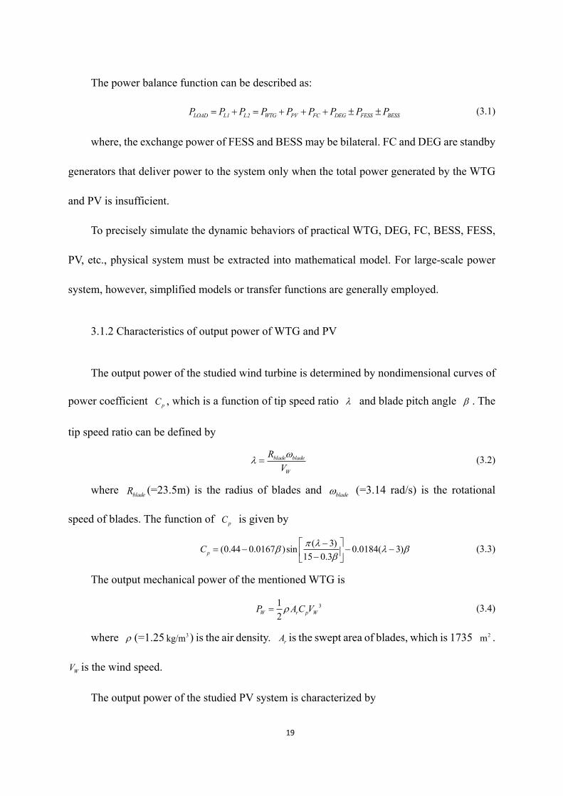
Figure 11.4 Solar radiation and PV output power

It can be seen that the output of WTG and output of PV will remain stable under constant

wind speed and smooth . Under the circumstance of little fluctuation of WTG output

and PV output, this thesis would mainly focus on the frequency response under obvious load

demand disturbance.

3.2.3 Simulation in Simulink

Simulink model of PI controller is shown as Figure 3.5.

F

WV F

25

Figure 12.5 Simulink scheme-PI

To illustrate the dynamic response of the MG system, the closed-loop system is examined

in the face of a multiple step load disturbance which is plotted in Figure 3.6 (a) and. And the

system frequency response using conventional PI controller is shown in Figure 3.6 (b). Besides,

conventional PI controllers are examined following a large step load disturbance of 0.1 pu as

shown in Figure 3.7.

(a)

26

(b)

Figure 13.6 (a) Multiple step load disturbances (b) MG frequency response

Figure 14.7 Frequency control following a step load disturbance of 0.1 pu

where, KP=0.3, KI=2. As shown in Figure 3.6 and Figure 3.7, the PI controller shows

robustness and keeps the frequency stable from load disturbance no matter it’s a single step

disturbance or multiple step disturbances. The adjust time is less than 2 seconds. But the initial

drop is still not satisfying, exceeding 0.05 pu.

In traditional power systems, the secondary frequency control is mostly done by

conventional PI controllers that are usually tuned based on prespecified operating points. In

27

case of any change in the operating condition, the PI controllers cannot provide the assigned

desirable performance. MPC can be used as a suitable intelligent method for online tuning of

PI controller parameters and may get better performance.

3.3 Model predictive control

3.3.1 Principle of MPC

Model predictive control technology has been widely used in SISO, MIMO and nonlinear

system [44-46]. MPC has serval advantages:1) handle the constraints in a systematic way, 2)

admirable implement of considering nonlinear system, 3) calculation time can be reduced to

get optimal control. The key feature of MPC is the model representation, which can be

described as state space, transfer matrix or convolution type models. Depending on the model,

computation and implementation will start automatically, processing the predicted value to

make control decision. We assume the system to be discussed in state space by

(3.15)

(3.16)

For zero-initial conditions, the equivalent transfer matrix representation is

(3.17)

(3.18)

where are the coefficients of impulse response. Thus, in the time domain, the output

can be calculated by

(3.19)

Then a cost function is defined determine the optimal control behavior at a certain

( ) ( ) ( )x k Ax k 1 Bu k 1= - + -

( ) ( )y k Cx k=

( ) ( ) ( )y z p z u z=

1 1

0 1

( ) ( I ) i i ii

i i

p z C z A B CA Bz H z¥ ¥

- - - -

= =

= - = =å å

iH

( )y k

1

( ) ( 1)ii

y k H u k¥

=

= -å

gf

28

time (control horizon). Depending on reference variable and predictive state variable

, can be designed as . The common function is square of the

difference between the reference variable and predictive state variable .

Naturally, control action which minimize the cost function is selected to control the system. In

general, the most important part in MPC algorithm is the state estimation function, which

directly influence the accuracy of predicted state values and may change the following control

action.

3.3.2 MPC controller for MG frequency control

In this thesis, MPC controller is proposed to control the DEG and FC generation

subsystem as a secondary control issue to maintain the stable frequency and power balance

under disturbance of load demand, comparing with the conventional PI controller. The MPC

framework for study is shown as Figure 3.8.

Figure 15.8 MPC framework

1( )kx t*+

1( )p kx t + gf 1 1{ ( ), ( )}i g k p kg f x t x t*+ +=

2

1 1( ) ( )i k p kg x t x t*+ += -

29

The goal is to control which should be equal to zero. is the output signal of MPC

to change the power of FC and DEG.

The state space function of former system can be expressed as:

(3.20)

(3.21)

(3.22)

(3.23)

where

(3.24)

(3.25)

(3.26)

(3.27)

and , , , , , are the deviation of frequency, the DEG system

output, the FC system output, the FESS system output, the BESS system output and load,

respectively. and are control signals from controller.

Cost function

fD u

( ) ( ) ( ) ( )( ) ( )

load WTG PVx t Ax t Bu t F P P Py t Cx t

= + + D +D +Dìí =î

!

( ) [ ]DEG DEG FC FC FC FESS BESSx t f P P P P P P P= D D D D D D D D! ! !!

( )y t f= D

1 2( ) [ ]u t u u= D D

1 1 1 10 0 02 2 2 2 2

1 10 0 0 0 0 0

1 10 0 0 0 0 0

1 10 0 0 0 0 0

1 10 0 0 0 0 0

10 0 0 0 0 0 0

1 10 0 0 0 0 0

1 10 0 0 0 0 0

t t

g g

c c

IN IN

FC

FESS FESS

BESS BESS

DH H H H H

T T

RT T

T TA

T T

T

T T

T T

é ù-ê úê úê ú-ê úê úê ú- -ê úê úê ú

-ê úê ú= ê ú

-ê úê úê ú

-ê úê úê úê ú-ê úê úê ú-ê úë û

1 10 0 0 0 0 0g FC

BT T

é ù= ê úê úë û

[1 0 0 0 0 0 0 0]C =

1[ 0 0 0 0 0 0 0]2

FH

= -

fD DEGPD FCPD FESSPD BESSPD loadPD

1uD 2uD

30

(3.28)

The first term minimizes the tracking error between the prediction of the measured system

frequency and its set-point , and the second term minimizes the control action effort.

are weighting factor value, which in this thesis have been selected to obtain similar SCS

bandwidth for MPC to that achieved for the other SCS strategies studied in this thesis.

are the minimum and maximum costing horizons, respectively, and is the control horizon.

are control signals processed by MPC.

Then, MPC controller can be given by

(3.29)

The MPC Simulink scheme is shown as Figure 3.9.

Figure 16.9 Simulink scheme-MPC

2

1

2 2 21 2 1 1 2 2

0 0

( , , ) [ ( ) 0] [ ( 1)] [ ( 1)]N Nu Nu

u

j N j j

J N N N t j t u t j u t jw l l= = =

= D + - + D + - + D + -å å å

nw 1 2,l l

1 2,N N

uN

1 2,u uD D

U KX= -

31

3.4 Case study

Power system operation states are changing in the real-time situation, which may degrade

the performance of the closed-loop microgrid system, distressingly. As indicated in the

previous sections, one of the main advantages of the advanced control methods is robustness

against environmental and dynamical changes. To illustrate the robustness of MPC control

strategy, three cases based on the different conditions of BESS and FESS are designed. In the

meanwhile, the simulation result of MPC controller will be compared with PI controller

mentioned before.

3.4.1 Case design

Microgrid can operate in both grid-connected and islanded operating modes to avoid huge

loss caused by external faults. The control schemes for MG system in islanded mode are more

complex and important than that in grid-connected mode; hence, an isolated ac MG system is

considered as a case study in this thesis. In addition, the changing state of FESS and BESS may

degrade the closed-loop system performance. Therefore, two binary variables are

proposed to describe the statuses of FESS and BESS system. If , the energy

storage systems operate in idle mode which means they reach their maximum capacity limit

and they can’t release or charge power furthermore at that status. And if , the

energy storage systems operate in connected mode with ability to respond to the dynamic

change of load power. According to the combination of those two variables, there are supposed

to be 4 cases. However, due to the same transfer function of FESS and BESS, there are three

cases shown as TABLE III.

,FESS BESSS S

, 0FESS BESSS S =

, 1FESS BESSS S =

32

TABLE III CASE STUDY DESIGN

Case study

Case1 1 1

Case2 0 0

Case3 1 0

3.4.2 Simulation result and discussion

Case1:

Figure 17.10 Case1 control system scheme

The block diagram of this studied case is shown as Figure 3.10. WTG and PV as renewable

sources are combined with DEG, FC, FESS and BESS. Power inverters are properly used in

various generation systems and energy storage systems to realize dc-ac transform. The

frequency error sign will be sent to both FC and DEG, processed by MPC controller to respond

to dynamic change of the connected load power. Assume that FC and DEG have their own

FESSS BESSS

33

MPC controller which means distributed control strategy, operating with others to obtain better

performance. In this case, uncertainty for the parameters which would influence the output of

WTG and PV generation is not considered. Besides, we assume that FESS and BESS have no

limit and they have enough capacity to store or release power in the system. Thus, they may

have faster speed for processing the frequency error signal produced by . So output

signals from BESS and FESS function are negative, to a certain degree, like a simple droop

control.

Figure 18.11 Frequency control following a step load disturbance of 0.1 p.u

There are two separate control signals from MPC sent to FC and DEG system to produce

corresponding power. The cooperation of two manipulated signals from MPC can obtain better

performance with less adjustment time.

where, sampling time is 0.01s, prediction horizon is 80 steps, control horizon is 4 steps,

.

The frequency response is shown as Figure 3.11.

oadLPD

1 2=0.1 =0.1l l，

34

Case2:


The block diagram of this studied case is shown as Figure 3.12. WTG and PV as renewable

sources are combined with DEG, FC. Power inverters are properly used in various generation

systems and energy storage systems to realize dc-ac transform. The frequency error sign will

be sent to both FC and DEG, processed by MPC controller to respond to dynamic change of

the connected load power. Assume that FC and DEG have their own MPC controller which

means distributed control strategy, operating with others to obtain better performance. In this

case, uncertainty for the parameters which would influence the output of WTG and PV

generation is not considered. Unlike case1, FESS and BESS lose their ability to respond

at high speed. In other words, they may just communicate with WTG and PV to charge or

release power directly. So BESS and FESS function can be removed in simulation.

oadLPD

35

Figure 20.13 Frequency control following a step load disturbance of 0.1 p.u


Case3:


The block diagram of this studied case is shown as above. Almost part of this case is the

same as case1 while the BESS are removed from the system. The FC and PV may generate dc

power that is converted into ac power using a dc–ac power converter. Again, the FESS have no

36

limit and they have enough capacity to store or release power in the system.


Figure 22.15 Case 3 frequency control following a step load disturbance of 0.1 p.u

Figure 23.16 Comparison for three cases

From Figure 3.11, Figure 3.13 and Figure 3.15, we can find that the MPC controller has

less overshoot and fast response speed. Frequency deviation in three case for MPC controller

are all less than 0.05 pu, reaching the desirable operation demand. It can be seen clearly that

case 1 has the best performance from Figure 3.16, since BESS and FESS have the ability to

supply insufficient generation subsystem within a short time. Besides, when BESS and FESS

37

loss their responsible ability, there is little difference between PI control method and MPC

control method (seen as case 2). In summary, through case study, it shows the advantage of

MPC control strategy in microgrid frequency control system and confirms its robustness under

dynamic change.

38

Chapter 4: MPC status feedback attack

4.1 Attack description

As mentioned in Chapter 3, various status feedback of FESS and BESS may

contribute to different performances of the closed-loop system. Due to the same transfer

function of FESS and BESS, there are three conditions related to the status of FESS and BESS,

illustrating whether they are connected to the system or not. All three conditions can achieve

frequency regulation, but the overshoot and response speed are totally different as they can be

distinguished easily. State estimation based on accuracy status feedback of the system

components is essential for the MPC controller to calculate corresponding control signal. If

status feedback of BESS and FESS are attacked by adversary, it may degrade the performance

of power system, causing huge of losses. For example, only BESS is available when the load

demand increases which means . However, after attacks is implemented in MPC,

the state estimator would receive the wrong information that both of FESS and BESS are still

on work to handle the power unbalance, which means . It may lead to risky

control strategy and terrific performance of system operation, producing impacts on reliability

and security of power grid. The scheme under MPC status feedback attack is depicted as Figure

4.1.

,FESS BESSS S

=1, =0FESS BESSS S

=1, =1FESS BESSS S

39

Figure 24.1 Scheme of MPC status feedback attack

From Figure 4.1, we can see that the hacker may get the access to attack state estimation of

MPC by injecting false data. Actually, the status feedback of WTG, PV, DEG and FC all can

be attacked. For simplicity, we only consider the attack to the statuses of FESS and BESS.

Further detection and online switching from different conditions are required to address status

feedback attack. We assume that if the frequency deviation is found to be different from what

it supposed to be, the state space of the system can be modified immediately. Then we need to

classify the actual situation among above three cases. New calculation and optimization

progress would be done automatically after the accuracy state space function and current states

of each components in the system are taken by the MPC controller.

40

4.2 Online switching method

Due to different statues of BESS and FESS, the state space functions that describe the dynamic

model of mentioned microgrid system vary from one to the other. Only with the accuracy state

space function, the state estimation can be processed properly, and the deviation of frequency

can be regulated. As the historical data of MPC output control signal are known, the

estimated frequency deviation of former three situations ( , ,

) can be obtained. Euclidean metric is proposed to measure the relativity of

current frequency deviation and the estimated frequency deviation. If we compare current data

and mentioned estimated data, we can detect the statuses of BESS and FESS where the less

error one can be recognized as actual statuses. Status feedback attack online detection block is

shown as Figure 4.2.

Figure 25.2 Status feedback attack online detection block

Although the state estimation is hacked by adversary at first, which may lead to terrific

u

=0, =0FESS BESSS S =1, =0FESS BESSS S

=1, =1FESS BESSS S

41

performance of system operation, a status feedback attack online detection is proposed to

address this problem. According to the state space function of each situation shown as status

block in Figure 4.2, can be calculated respectively during specific observation time.

Then RMSE (Root Mean Squared Error) block is utilized to measure the error when comparing

with . Then the less error one is approximately considered as current updated

status feedback of BESS and FESS. Therefore, the MPC controller is modified by updated

status feedback in real time. In next control step, predicted states and control signal are

computed by the updated state space function of actual model related to statuses of BESS and

FESS.

4.3 Case study

In this case, FESS and BESS system are in idle mode ( ) which means they reach

their maximum capacity limit and they can’t release or charge power furthermore at that status.

However, the state estimations of FESS and BESS system are hacked by the intruder, resulting

the status feedback from BESS and FESS to be . As the MPC controller takes the

wrong status feedback, control signal would be totally different from what it should be in the

regular operation. Therefore, inevitable damage and insufficient control function may be

occurred in the respect of dynamic model of frequency secondary control based on MPC.

1 2 3, ,f f fD D D

1 2 3, ,f f fD D D fD

=0, =0FESS BESSS S

=1, =1FESS BESSS S

42

Figure 26.3 Frequency response under status feedback attack

The frequency response of mentioned case with 0.1 pu load disturbance at t=2s is depicted as

Figure 4.3, which is simulated in MATLAB. It can be seen that such status feedback attack

would cause system instability and slightly obtain the expectation of frequency control.

Then, the proposed online detection and switching method with 0.1 pu load disturbance at t=2s

is implemented in simulation. The result of system frequency response and online detection of

statues of BESS and FESS are shown as Figure 4.5 and Figure 4.6, respectively. From Figure

4.4 and Figure 4.5, we can verify the effectiveness of the proposed method to achieve frequency

regulation with the MPC controller as secondary control part. In Figure 4.6, when t=2.05s, the

algorithm can detect the accuracy status feedback of FESS and BESS, where BESS, FESS=00

represents . Therefore, the MPC controller can modify the state estimation with

the original states of FESS and BESS.

=0, =0FESS BESSS S

43

Figure 27.4 Frequency response with online switching method under status feedback attack

Figure 28.5 Online detection of statues of BESS and FESS

44

Chapter 5: Modified MPC controller under time-delay attack

5.1 Time delay attack

Modern power grids rely on open communication infrastructure to improve the efficiency,

sustainability and reliability of three levels of power system (generation, transmission and

distribution), which makes them vulnerable to cyber-attacks implemented by adversary. In

general, an intruder attempts to get into IT infrastructure of control system and manipulate

various sensors to disrupt control signals. For example, an intruder can shut down a load on a

specific power transformer or introduce inefficiencies in the power supply.

Many efforts have culminated in a huge number of literature, including stability analyzing

method of attacks on industrial control systems, updating hardware and software systems and

advanced measurement units to prevent potential attacks from destroying secure operation. An

identifying method for a change in sets of inferred candidate invariants under FDI attack is

proposed in [47]. Literature [48] studies the impact of FDI on distributed load sharing. In [49],

Markov based state transition rules is presented to simulate microgrid responses considering

the behavior of PV and ESS control systems. Authors in [50] consider how a time-delay attack

affects the dynamic performance of a power system.

Commonly, the local information measured by sensors is sent to the communication

channel. Then state estimator starts to calculate current states which is essential for making

control decision in control center. After receiving the signal from control center, frequency

controller can send the control signal to all kinds of DEG through the communication channel.

Due to the high dependence of communication infrastructure, the system would be vulnerable

45

to various attack risks. A simplified load frequency control system under time-delay attack is

depicted in Figure 5.1. However, most of recent studies considered either the construction of

controllers that are robust to time delays or controllers that train offline with a time-delay

function for estimation. As far as it is known, there are few control methods that perform online

estimation of dynamic time delays and real-time control of power systems.

Figure 29.1 A simplified load frequency control system under time-delay attack

46

5.2 MPC controller under time-delay attack

5.2.1 Modelling

Figure 30.2 Dynamic model of MPC frequency control with delay attack

The model of conventional MPC control scheme is modified, shown in Figure 5.2,

considering the time delay attack in the control loop.

Figure 31.3 MPC control block diagram under attack

The deviation of frequency of plant output, which is detected by sensor (PLL in microgrid),

will be compared to reference signal r. However, the sensed data will be delayed due to time-

delay attack, causing different state estimation of MPC controller. Then the control signal u is

47

not corresponding to real system state, and fluctuation of frequency and undesirable

performance would occur.

The state space function of former system can be expressed as same as formula 3.20.

Besides, as shown by an exponential block , is the estimated time delay of the system.

With the time-delay attack, the control signal will be modified by

(5.1)

And the new state after attack can be modeled by

(5.2)

Since a time-delay attack can sabotage and ruin the network control system to cause huge

loss, control strategies must be developed that must be able to detect and track the time-delay

attack and manage a response strategy.

5.2.2 Case study with known time-delay signal

In this case, time delay is assumed to be known in system. Under four different delay

time and 0.1 pu load disturbance at 2s, the frequency respond of microgrid system with MPC

controller is shown as Figure 5.4, Figure 5.5, Figure 5.6 and Figure 5.7.

se t- t

ˆU KX= -

1 1 1

2 2 2

8 8 8

ˆ ( )ˆ ( )ˆ

ˆ ( )

x x tx x t

X

x x t

tt

t

-é ù é ùê ú ê ú-ê ú ê ú= =ê ú ê úê ú ê ú-ë û ë û

! !

t

48

Figure 32.4 Frequency respond when =0.1s



t

t

t

49


where, sampling time is 0.01s, prediction horizon is 80 steps, control horizon is 4 steps,

.

It can be seen clearly that MPC controllers will obtain better performance (less overshoot,

faster adjust time, stable curve) of microgrid frequency control than PI controllers with

increasing delay time. Even when is larger than 0.6s, the frequency respond of PI controller

will be divergent. Under the situation of known time-delay, MPC controllers are promising.

However, in the real power system, it’s impossible to get the exact information of time-delay

attack by adversary instant immediately, or time-delay attack can be time-varying. Therefore,

it’s indispensable to set up a new algorithm to prevent time-delay attack on microgrid frequency

control system in real-time.

t

1 2=0.1 =0.1l l，

t

50

5.3 Modified MPC with online time-delay estimation

5.3.1 Methodology

The new method involves the use of the plant model, a time-delay estimator, and the MPC

controller to control system frequency under TDS attack. The control scheme will detect and

track time delays introduced by a hacker and guide the plant to track the reference signal to

guarantee the stability for the system. Figure 5.8 shows the diagram of proposed control method.

Figure 36.8 Block diagram of proposed control technique

This thesis proposes a GCC (generalized cross correlation) time-delay estimator to update

delay estimation. Then the state space can be modified with estimated time-delay. According

to the updated plant model, MPC controller could adjust their control signal to eliminate the

fluctuation caused by unknown delay attack.

For simplification, the system being dealt with can be approximated in state space function,

which takes plant block directly to describe the dynamic of system.

(5.3)

( ) ( ) ( ) ( )f t x t Ax t Bu tD = = +! !

51

and its solution is given by

(5.4)

Due to the time-delay attack from the attacker, the solution becomes

(5.5)

In general, the time delay is an unknown variable. No matter it is a constant or time-

varying value, we want to estimate the time delay .

It should be noted that is actually measured from sensor. So, at every instance of

time, variable and are known to the controller and the plant model. On the

other hand, the current and the time delay are unknown. It is essential to estimate the

time delay firstly and then estimates correctly.

Assume that former state can be obtained at every time step. The plant model estimation

equation is given by

(5.6)

Through the plant model estimation, we can calculate the estimated state value since

are known and former processed by MPC controller are saved. Then, GCC

estimator can be used to estimate time delay by comparing and . So it’s

definitely important to get the plant model state estimation in order to estimate time delay attack

to the communication channel.

5.3.2 Generalized cross correlation

GCC algorithm is widely used in field of signal processing to estimate the time delay

between two signals [51-52]. In some sense, the output signal from sensors and state estimate

( )0 0

( ) ( )tAt A t sx t e x e Bu s ds-= + ò

( ) ( )0 0

( ) ( )tA t A t sx t e x e Bu s dstt tt-- - -- = + ò

t

t

( )x t t-

( ), ,u t A B ( )x t t-

( )x t

t ( )x t

ˆ ˆ( ) ( ) ( ) loadx t Ax t Bu t F P= + + D!

ˆ( )x t

, , , loadA B F PD ( )u t

t ˆ( )x t ( )x t t-

52

signal are two related signals, which can also use GCC to detect and track time delay.

For convenient, and can be mathematically remarked as

(5.7)

(5.8)

where is real signal obtained from sensor, is noise signal. Signal is

assumed to be uncorrelated with .

Here, the cross-correlation function is proposed to determine the time delay D as formula

5.9.

(5.9)

where E denotes expectation，T is observation interval. The peak of cross correlation

function provides an estimate of delay. GCC is aimed to improve the accuracy of the delay

estimate where and are filtered. Therefore, the generalized cross correlation

function based on the phase transform (PHAT) between and is

(5.10)

(5.11)

Ideally, the PHAT weighting function delivers an ideal GCC:

(5.12)

(5.13)

5.3.3 Algorithm of controller design

Step 1: Initialize time-delay estimate , plant model state estimate , reference signal r

and MPC controller state xmpc.

ˆ( )x t ( )x t t-

1 1( ) ( ) ( ) ( )y t x t s t n tt= - = +

2 1ˆ( ) ( ) ( )y t x t s t D= = +

1( )s t ( )n t 1( )s t

( )n t

1 2 1 2 1 21( ) [ ( ) ( )] ( ) ( )

T

y yR E y t y t y t y t dtT t

t t tt

= - = -- ò

D̂ 1( )y t 2( )y t

1( )y t 2( )y t

1 2 1 2

( ) 2( ) ( ) ( )y y y y

g j fgR f G f e dfp tt j

¥

-¥= ò

1 2

1( )( )

y y

g fG f

j =

1 2

( ) ( ) ( )y y

gR t Dt d= -

( )ˆ ( ( ))y y1 2

argmax gdD R t=

t̂ x̂

53

Step 2: Obtain a plant state measurement (i.e., the sensed output states of the plant

), which could be hacked by attackers.

Step 3: Compute the current state estimate, , according to the plant state space model.

The discrete equation can be approximated as:

Step 4: Use GCC algorithm to compute the time-delay estimate by comparing

historical data and . In order to reduce the computation complexity, an

observation interval T is utilized to compute the cross-correlation function.

Step 5: Modify MPC controller state model with time-delay estimate obtained in step

3. And then compute the new MPC controller state xmpc.

Step 6: Compute the control signal in the MPC controller. As new MPC controller

state xmpc and the input of MPC controller are known, can be set by MPC

algorithm.

Step 7: To prevent runaway and dead-zone situations, bound time-delay estimate by

and the control signal by .

Step 8: Repeat step 2-7 in the case of tracking a reference trajectory r.

( )x t t-

ˆ( )x t

ˆ ˆ( +1) ( ) ( ) ( )loadx k Ax k Bu k F P k= + + D!

t̂

ˆ( )x t ( )x t t-

t̂

( )u t

( ) ( ) ( )e t r t x t t= - - u

maxt

maxu±

54

Chapter 6: Case study

6.1 Modified MPC model simulation

To verify the effectiveness and advantages of modified MPC control strategy, three cases

are designed to analyze the microgrid frequency response:

1). A constant time-delay attack is applied into system with 0.1 pu load increase

2). A time-varying delay attack is applied into system with 0.1 pu load increase

3). A time-varying delay attack is applied into system with changing load disturbance

By simulating those three cases, the time window of GCC is set as 2s and the MPC

controller will be implemented in MATLAB.

6.1.1 Case 1: constant time-delay attack

In this case, the system works in islanded mode. Then, load power increases 0.1 pu since

t=2s, and a 0.2s constant time-delay attack is applied into communication channel. Taking the

modified MPC control method, online delay estimation and the system frequency control

performance is shown Figure 6.1 and Figure 6.2, respectively.

55

Figure 37.1 GCC delay estimation in case1

Figure 38.2 Frequency response following a step load disturbance of 0.1 pu

From Figure 6.1, we can see that GCC estimation method can detect and track the time-

delay attack with approximately 0.5s error, which is quite appealing. Thus, after acquiring

accurate delay time, the state estimation in MPC can work as condition. It can be observed in

Figure 6.2 that modified MPC algorithm based on GCC estimation can make system frequency

56

stable with less than 3s adjustment time and 0.02 pu overshoot. On the other side, traditional

MPC needs 10s to realize secondary frequency control and has worse control performance.

6.1.2 Case 2: time-varying delay attack

Case 2 are almost similar to Case 1, except for the delay attack signal. In this case, time

delay is 0.2s from t=2s to t=3s and it changes to 0.4s after t=3s. Figure 6.3 shows the frequency

output of system and time-varying delay estimation. Load power increases 0.1 pu since t=2s,

causing a frequency decrease by the function as droop control at first. Therefore, MPC as a

secondary frequency control scheme is designed to balance the power generation and load

demand to control the frequency.

Figure 39.3 (a) Frequency output of microgrid system in case 2 (b) time-varying delay estimation

It shows that modified MPC algorithm based on GCC estimation can also obtain satisfying

performance under time-varying delay. The frequency of system maintains stable after t=5s

57

and the overshoot is about 0.02 pu. Under this circumstance, even when the time-delay attack

changes with a short interval, the proposed method will compensate the frequency deviation as

the function of secondary frequency control system.

6.1.3 Case 3: two steps load disturbance

In this case, load disturbance has two steps where it’s 0.1 pu from t=2s to t=10s and 0.2

pu after t=10s, which is shown in Figure 6.4. On the other hand, time delay is 0.2s from t=2s

to t=10s and it changes to 0.4s after t=10s. Figure 6.5 and Figure 6.6 show time-varying delay

estimation and the frequency response of microgrid system, respectively.

Figure 40.4 Two steps load disturbance

58

Figure 41.5 GCC time delay estimation in case 3

Figure 42.6 Frequency response in case 3

From Figure 6.5, GCC estimation can track the original time-delay attack correctly with

little deviation. From Figure 6.6, we can see that there are two peaks when =0.4s, which

would be higher than =0.2s. In other words, due to the longer delay time, the latter control

t

t

59

process is more severe than the former period. But the result can still verify the effectiveness

of modified MPC control method under two steps load disturbance with time-varying delay

attack.

6.2 Discussion

After analyzing the results of the three case studies mentioned above, we can gain the

following conclusions:

(1) The proposed modified MPC can handle the risk under constant and time-varying

delay, managing short-term load disturbance successfully. Time-delay attack can be detected

and time-delay tracked by GCC method.

(2) The modified MPC control strategy can keep the frequency of microgrid stable under

different load disturbance and various time delay attack (e.g. one changing fast in a short time)

in real-time operation.

(3) The key part of Modified MPC control strategy is the GCC time-delay estimator, which

directly influence the model description and performance of dynamic system. The maximum

of time delay attack that the proposed method can handle is 0.8s, otherwise the frequency

deviation will be divergent.

(4) After some experiments, various observation time of GCC, during which cross

correlation function is calculated to obtain time delay estimation, may lead to different

estimation results.

60

Chapter 7: Conclusion and future work

7.1 Conclusion

In this thesis, the hierarchical structure of microgrid control systems is studied by

introducing primary, secondary, and tertiary controls to address different significances and time

scales among microgrid control demand. We focus on the secondary frequency control system.

The studied islanded microgrid consists of DEG, PV panel, WTG, FC system, BESS, and FESS.

All above components can be described by transfer function as a first-order model. Then, the

conventional PI controller is simulated in Simulink to compensate frequency deviation under

load disturbance. However, in case of any change in the operating conditions, the PI controllers

cannot provide the assigned desirable performance. MPC is applied as a suitable intelligent

method to compare with the PI controller. The results simulated in MATLAB show that the

MPC controller has less overshoot and faster response speed, reaching the desirable operation

demand. Three case studies in Chapter 3 verify the robustness of the MPC controller under

dynamic change.

On the other side, we find that BESS and FESS have the ability to supply insufficient

generation subsystems within a short time. When BESS and FESS lose their responsible ability,

there is trifling difference between the PI control method and the MPC control method. The

status feedback attack to the MPC controller is considered. The wrong status feedback of BESS

and FESS systems may lead to unrecoverable instability to the microgrid system. Therefore,

an online switching method based on RMSE is proposed to identify the original status feedback

61

of BESS and FESS. A simple case study is designed to analyze the detriment caused by the

status feedback attack and to verify the effectiveness of the proposed method to protect the

control system from such an attack.

Regarding the cyber-security of the microgrid system, time delay attack occurred in the

communication channel by an adversary is mainly discussed. To prevent the secondary

frequency control of the microgrid system from time-delay attacks, a modified MPC method

based on GCC estimation is proposed. During the online operation, time delay can be estimated

by GCC and then the state estimation in MPC controller can update. According to the updated

plant model, the MPC controller could adjust its control signal to eliminate the fluctuation

caused by unknown delay attacks. Finally, the proposed modified MPC can detect and track

both constant and time-varying delays, keeping the frequency of the system successfully stable.

7.2 Future work

In this section, recommendations for future work are listed.

1. Various observation time of GCC, during which cross correlation function is

calculated to obtain time delay estimation, may lead to different estimation results. In this

thesis, the observation time of GCC is set as 2s. Besides, the maximum of time delay

attack under proposed method is 0.8s. In the future, some adjustment should be made in

improving the accuracy of GCC estimation.

2. In this thesis, only the LTI system in state feedback was discussed, though the method

is general in essence. In the future research, the method will be verified that it also works

for a class of nonlinear systems.

3. In this thesis, the simulation model assumes that the wind speed and solar radiation

62

remain a smooth curve. However, in the real microgrid system, we need to consider the

disturbance of wind speed and solar radiation. For my future work, more case studies

considering fluctuations of wind speed and solar radiation will be designed.

63

REFERENCES

[1] International Energy Agency. World Energy Outlook. https://www.iea.org/weo2018/ .

[2] N. Hatziargyriou, H. Asano, R. Iravani, and C. Marnay, “Microgrids,” IEEE Power Energy Mag.,

vol. 5, no. 4, pp. 78–94, Jul./Aug. 2007.

[3] T. Ustun, C. Ozansoy, A. Zayegh. Recent developments in microgrids and example cases around

the world. A review. Renew Sustain Energy Rev2011;15(8):4030–41.

[4] K. Alanne, A. Saari. Distributed energy generation and sustainable development. Renew Sustain

Energy Rev 2006;10(6):539–58.

[5] C.M. Closon, M.H. Nehrir, Algorithms for distributed decision-making for multi-agent microgrid

power management. In Proceedings of the IEEE Power and Energy Society General Meeting,

Detroit, MI, USA,24–29 July 2011; pp. 1–8.

[6] M. E. Khodayar, M. Barati, and M. Shahidehpour, “Integration of high reliability distribution

system in microgrid operation,” IEEE Trans.Smart Grid, vol. 3, no. 4, pp. 1997–2006, Dec. 2012.

[7] R. Lasseter and P. Piagi, “Microgrid: A conceptual solution,” in Proc. IEEE Annu. Power Electron

Specialists Conf., Jun. 2004, pp. 4285–4290.

[8] (Mar.2019). Industrial control systems are still vulnerable to malicious cyberattacks [online].

Available: https://www.technologyreview.com/s/612829/industrial-control-systems-are-still-

vulnerable-to-malicious-cyberattacks/

[9] (Mar.2019). Cybersecurity for Critical Infrastructure Protection. [Online]. Available:

https://www.gao.gov/new.items/d04321.pdf

[10] R. McMillan, “Siemens: Stuxnet worm hit industrial systems,” COMPUTER World, Sept. 2010.

64

[11] R.M. Lee, M.J. Assante, T. Conway, Analysis of the Cyber Attack on the Ukrainian Power Grid;

Electricity Information Sharing and Analysis Center (E-ISAC): Washington, DC, USA, 18 March

2016.

[12] K. Manandhar, X. Cao, F. Hu and Y. Liu, "Detection of Faults and Attacks Including False Data

Injection Attack in Smart Grid Using Kalman Filter," in IEEE Transactions on Control of Network

Systems, vol. 1, no. 4, pp. 370-379, Dec. 2014.

[13] Y. Liu, P. Ning, and M. K. Reiter, “False data injection attacks against state estimation in electric

power grids,” ACM Trans. Inf. Syst. Security, vol. 14, no. 1, p. 13, 2011.

[14] I. Kamwa, R. Grondin, and Y. Hebert, “Wide-area measurement based stabilizing control of large

power systems—A decentralized/hierarchical approach,” IEEE Trans. Power Syst., vol. 16, no. 1,

pp. 136–153, Feb. 2001.

[15] H. X. Wu, K. S. Tsakalis, and G. T. Heydt, “Evaluation of time delay effects to wide-area power

system stabilizer design,” IEEE Trans. Power Syst., vol. 19, no. 4, pp. 1935–1941, Nov. 2004.

[16] Q. Jiang, Z. Zou, and Y. Cao, “Wide-area TCSC controller design in consideration of feedback

signals’ time delays,” in Proc. IEEE Power Eng. Soc.Gen.Meeting, vol. 2. San Francisco,CA, USA,

2005, pp. 1676–1680.

[17] Y.L. Huang, A.A. Cárdenas, S. Amin, Z.S. Lin, H.Y. Tsai, S. Sastry, Understanding the physical

and economic consequences of attacks on control systems, International Journal of Critical

Infrastructure Protection, Volume 2, Issue 3, 2009, Pages 73-83, ISSN 1874-5482.

[18] D. Dotta, A. S. e Silva, and I. C. Decker, “Wide-area measurementsbased two-level control design

considering signal transmission delay,” IEEE Trans. Power Syst., vol. 24, no. 1, pp. 208–216, Feb.

2009.

65

[19] C.-K. Zhang, L. Jiang, Q. H. Wu, Y. He, and M. Wu, “Delay-dependent robust load frequency

control for time delay power systems,” IEEE Trans. Power Syst., vol. 28, no. 3, pp. 2192–2201,

Aug. 2013.

[20] A. Sargolzaei, K. K. Yen and M. N. Abdelghani, "Preventing Time-Delay Switch Attack on Load

Frequency Control in Distributed Power Systems," in IEEE Transactions on Smart Grid, vol. 7, no.

2, pp. 1176-1185, March 2016.

[21] L. Jiang, W. Yao, Q. H. Wu, J. Y. Wen and S. J. Cheng, "Delay-Dependent Stability for Load

Frequency Control With Constant and Time-Varying Delays," in IEEE Transactions on Power

Systems, vol. 27, no. 2, pp. 932-941, May 2012.

[22] D. E. Olivares et al., "Trends in Microgrid Control," in IEEE Transactions on Smart Grid, vol. 5,

no. 4, pp. 1905-1919, July 2014.

[23] J. M. Guerrero, J. C. Vasquez, J. Matas, L. G. de Vicuña, and M. Castilla, “Hierarchical control of

droop-controlled AC and DC microgrids—A general approach towards standardization,” IEEE

Trans. Ind. Electron., vol. 58, no. 1, pp. 158–172, Jan. 2011.

[24] J. A. P. Lopes, C. L. Moreira, and A. G. Madureira, “Defining control strategies formicrogrids

islanded operation,” IEEE Trans. Power Syst., vol. 21, pp. 916–924, May 2006.

[25] A. Bidram and A. Davoudi, "Hierarchical Structure of Microgrids Control System," in IEEE

Transactions on Smart Grid, vol. 3, no. 4, pp. 1963-1976, Dec. 2012.

[26] H. Karimi, E. J. Davison, and R. Iravani, “Multivariable servomechanism controller for

autonomous operation of a distributed generation unit: Design and performance evaluation,” IEEE

Trans. Power Syst., vol. 25, no. 2, pp. 853–865, May 2010.

66

[27] B. Bahrani, M. Saeedifard, A. Karimi, and A. Rufer, “A multivariable design methodology for

voltage control of a single-DG-unit microgrid,” IEEE Trans. Ind. Electron., vol. 9, no. 2, pp. 589–

599, May 2013.

[28] T. L. Vandoorn, J. D. M. De Kooning, B. Meersman, J. M. Guerrero, and L. Vandevelde, “Voltage-

based control of a smart transformer in a microgrid,” IEEE Trans. Ind. Electron., vol. 60, no. 4, pp.

1291–1305, Apr. 2013.

[29] T. Iwade, S. Komiyama, and Y. Tanimura, “A novel small-scale UPS using a parallel redundant

operation system,” in Proc. Int. Telecommunications Energy Conf., 2003, pp. 480–483.

[30] J. A. P. Lopes, C. L. Moreira, and A. G. Madureira, “Defining control strategies formicrogrids

islanded operation,” IEEE Trans. Power Syst., vol. 21, no. 2, pp. 916–924, May 2006.

[31] Y. J. Cheng and E. K. K. Sng, “A novel communication strategy for decentralized control of

paralleled multi-inverter systems,” IEEE Trans. Power Electron., vol. 21, pp. 148–156, Jan. 2006.

[32] F. Katiraei, M. R. Iravani, and P. W. Lehn, “Micro-grid autonomous operation during and

subsequent to islanding process,” IEEE Trans. Power Del., vol. 20, no. 1, pp. 248–257, Jan. 2005.

[33] H. Bevrani, Robust Power System Frequency Control. New York: Springer, 2009.

[34] S. Obara, “Analysis of a fuel cell micro-grid with a small-scale wind turbine generator,” Int. J.

Hydrogen Energy, vol. 32, pp. 323–336, Mar.2007.

[35] Bidram, A. Davoudi, F. L. Lewis, and J. M. Guerrero, “Distributed cooperative secondary control

of microgrids using feedback linearization,” IEEE Trans. Power Syst., vol. 28, no. 3, pp. 3462–

3470, Aug. 2013.

[36] R. Palma-Behnke et al., “A microgrid energy management system based on the rolling horizon

strategy,” IEEE Trans. Smart Grid, vol. 4, no. 2, pp. 996–1006, Jun. 2013.

67

[37] Y. Khayat et al., "Decentralized Optimal Frequency Control in Autonomous Microgrids," in IEEE

Transactions on Power Systems. 2018.

[38] J. M. Rey, P. Marti, M. Velasco, J. Miret, and M. Castilla, “Secondary Switched Control with no

Communications for Islanded Microgrids,” IEEE Trans. Ind. Electron., pp. 8534–8545, 2017.

[39] R. Han, L. Meng, J. M. Guerrero, and J. C. Vasquez, “Distributed Nonlinear Control with Event-

Triggered Communication to Achieve Current-Sharing and Voltage Regulation in DC Microgrids,”

IEEE Trans. Power Electron., pp. 1–1, 2017.

[40] W. Gu, G. Lou, W. Tan, and X. Yuan, “A Nonlinear State Estimator-Based Decentralized

Secondary Voltage Control Scheme for Autonomous Microgrids,” IEEE Trans. Power Syst., pp.

4794–4804, 2017.

[41] H. Bevrani, F. Habibi, P. Babahajyani, M. Watanabe and Y. Mitani, "Intelligent Frequency Control

in an AC Microgrid: Online PSO-Based Fuzzy Tuning Approach," in IEEE Transactions on Smart

Grid, vol. 3, no. 4, pp. 1935-1944, Dec. 2012.

[42] J. M. Guerrero, L. Hang, and J. Uceda, “Control of distributed uninterruptible power supply

systems,” IEEE Trans. Ind. Electron., vol. 55, pp. 2845–2859, Aug. 2008.

[43] T. Senjyu, T. Nakaji, K. Uezato, and T. Funabashi, “A hybrid power system using alternative

energy facilities in isolated island,” IEEE Trans. Energy Convers., vol. 20, no. 2, pp. 406–414, Jun.

2005.

[44] S. Kouro, P. Cortes, R. Vargas, U. Ammann and J. Rodriguez, "Model Predictive Control—A

Simple and Powerful Method to Control Power Converters," in IEEE Transactions on Industrial

Electronics, vol. 56, no. 6, pp. 1826-1838, June 2009.

68

[45] M. B. Shadmand, R. S. Balog and H. Abu-Rub, "Model Predictive Control of PV Sources in a

Smart DC Distribution System: Maximum Power Point Tracking and Droop Control," in IEEE

Transactions on Energy Conversion, vol. 29, no. 4, pp. 913-921, Dec. 2014.

[46] G. Grimm, M. J. Messina, S. E. Tuna and A. R. Teel, "Nominally Robust Model Predictive Control

With State Constraints," in IEEE Transactions on Automatic Control, vol. 52, no. 10, pp. 1856-

1870, Oct. 2007.

[47] O. A. Beg, T. T. Johnson and A. Davoudi, "Detection of False-Data Injection Attacks in Cyber-

Physical DC Microgrids," in IEEE Transactions on Industrial Informatics, vol. 13, no. 5, pp. 2693-

2703, Oct. 2017.

[48] H. Zhang, W. Meng, J. Qi, X. Wang and W. X. Zheng, "Distributed Load Sharing Under False

Data Injection Attack in an Inverter-Based Microgrid," in IEEE Transactions on Industrial

Electronics, vol. 66, no. 2, pp. 1543-1551, Feb. 2019.

[49] X. Liu, M. Shahidehpour, Y. Cao, L. Wu, W. Wei and X. Liu, "Microgrid Risk Analysis

Considering the Impact of Cyber Attacks on Solar PV and ESS Control Systems," in IEEE

Transactions on Smart Grid, vol. 8, no. 3, pp. 1330-1339, May 2017.

[50] A. Sargolzaei, K. Yen and M. Abdelghani, "Delayed inputs attack on load frequency control in

smart grid," ISGT 2014, Washington, DC, 2014, pp. 1-5.

[51] C. Knapp and G. Carter, "The generalized correlation method for estimation of time delay," in

IEEE Transactions on Acoustics, Speech, and Signal Processing, vol. 24, no. 4, pp. 320-327,

August 1976.

69

[52] M. Azaria and D. Hertz, "Time delay estimation by generalized cross correlation methods," in

IEEE Transactions on Acoustics, Speech, and Signal Processing, vol. 32, no. 2, pp. 280-285, April

1984.

Model Predictive Control Design for the Secondary ...

Documents

Transcript of Model Predictive Control Design for the Secondary ...