MODEL ORDER REDUCTION OF NONLINEAR DYNAMIC SYSTEMS …
203
MODEL ORDER REDUCTION OF NONLINEAR DYNAMIC SYSTEMS USING MULTIPLE PROJECTION BASES AND OPTIMIZED STATE-SPACE SAMPLING by José A. Martínez B.S. in Electrical Engineering, Universidad de Oriente, Barcelona, 1993 M.S. in Electrical Engineering, University of Pittsburgh, Pittsburgh, 2000 Submitted to the Graduate Faculty of Swanson School of Engineering in partial fulfillment of the requirements for the degree of PhD in Electrical Engineering University of Pittsburgh 2009
Transcript of MODEL ORDER REDUCTION OF NONLINEAR DYNAMIC SYSTEMS …

MODEL ORDER REDUCTION OF NONLINEAR DYNAMIC SYSTEMS USING
MULTIPLE PROJECTION BASES AND OPTIMIZED STATE-SPACE SAMPLING
by
José A. Martínez
B.S. in Electrical Engineering, Universidad de Oriente, Barcelona, 1993
M.S. in Electrical Engineering, University of Pittsburgh, Pittsburgh, 2000
Submitted to the Graduate Faculty of
Swanson School of Engineering in partial fulfillment
of the requirements for the degree of
PhD in Electrical Engineering
University of Pittsburgh
2009

ii
UNIVERSITY OF PITTSBURGH
SWANSON SCHOOL OF ENGINEERING
This dissertation was presented
by
José A. Martínez
It was defended on
June 06, 2008
and approved by
James T. Cain, Professor Emeritus, Electrical Engineering
Amro A. El-jaroudi, Associate Professor, Electrical Engineering
Donald M. Chiarulli, Professor, Computer Science
Rob Rutenbar, Professor, ECE, Carnegie Mellon
Dissertation Director: Steven P. Levitan, Professor, Electrical Engineering

iii
Copyright © by José A. Martínez
2009

iv
Model order reduction (MOR) is a very powerful technique that is used to deal with the
increasing complexity of dynamic systems. It is a mature and well understood field of study that
has been applied to large linear dynamic systems with great success. However, the continued
scaling of integrated micro-systems, the use of new technologies, and aggressive mixed-signal
design has forced designers to consider nonlinear effects for more accurate model
representations. This has created the need for a methodology to generate compact models from
nonlinear systems of high dimensionality, since only such a solution will give an accurate
description for current and future complex systems.
The goal of this research is to develop a methodology for the model order reduction of
large multidimensional nonlinear systems. To address a broad range of nonlinear systems, which
makes the task of generalizing a reduction technique difficult, we use the concept of
transforming the nonlinear representation into a composite structure of well defined basic
functions from multiple projection bases.
We build upon the concept of a training phase from the trajectory piecewise-linear
(TPWL) methodology as a practical strategy to reduce the state exploration required for a large
nonlinear system. We improve upon this methodology in two important ways: First, with a new
strategy for the use of multiple projection bases in the reduction process and their coalescence
into a unified base that better captures the behavior of the overall system; and second, with a
MODEL ORDER REDUCTION OF NONLINEAR DYNAMIC SYSTEMS USING
MULTIPLE PROJECTION BASES AND OPTIMIZED STATE-SPACE SAMPLING
José A. Martínez, PhD
University of Pittsburgh, 2009

v
novel strategy for the optimization of the state locations chosen during training. This
optimization technique is based on using the Hessian of the system as an error bound metric.
Finally, in order to treat the overall linear/nonlinear reduction task, we introduce a
hierarchical approach using a block projection base. These three strategies together offer us a
new perspective to the problem of model order reduction of nonlinear systems and the tracking
or preservation of physical parameters in the final compact model.
DESCRIPTORS
Compact Model Generation
Nonlinear Model Order Reduction
Model Order Reduction
TPWL Methodology
vi
TABLE OF CONTENTS
ACRONYMS AND SYMBOLS.............................................................................................. XIV
ACRONYMS.................................................................................................................... XIV
SYMBOLS..........................................................................................................................XV
ACKNOWLEDGMENTS ....................................................................................................... XVI
1.0 INTRODUCTION........................................................................................................ 1
1.1 PROBLEM STATEMENT................................................................................. 5
1.2 STATEMENT OF WORK.................................................................................. 7
1.3 CONTRIBUTIONS ........................................................................................... 13
1.4 DISSERTATION ROAD MAP ........................................................................ 15
2.0 MODEL ORDER REDUCTION.............................................................................. 18
2.1 A BRIEF HISTORY.......................................................................................... 18
2.2 MODEL ORDER REDUCTION ..................................................................... 22
2.3 MOR OF LINEAR SYSTEMS......................................................................... 23
2.3.1 Polynomial Approximations of the Transfer Function/ Explicit Moment Matching techniques ........................................................ 24
2.3.2 State Truncation Approach........................................................................... 26
2.3.3 Subspace Projection techniques.................................................................... 30
2.3.4 Proper Orthogonal Decomposition............................................................... 33
2.4 MODEL ORDER REDUCTION OF NONLINEAR SYSTEMS.................. 36
2.4.1 Linearization Methods................................................................................... 37
2.4.2 Quadratic Methods ........................................................................................ 38
2.4.3 Piecewise Linear Model Order Reduction................................................... 40

vii
2.4.4 High order Piecewise Model Order Reduction ........................................... 42
2.4.5 Proper Orthogonal Decomposition............................................................... 42
2.5 SUMMARY........................................................................................................ 44
3.0 BLOCK PROJECTION TECHNIQUE FOR MODEL ORDER REDUCTION ............................................................................................................. 45
3.1 LINEAR SYSTEM REDUCTION USING BLOCK PROJECTION ................................................................................................... 46
3.2 SUB-BLOCK NONLINEAR SYSTEM REDUCTION USING BLOCK PROJECTION.................................................................................... 47
3.3 SUMMARY........................................................................................................ 50
4.0 DEVELOPMENT OF A MATLAB BASED ANALOG SOLVER FOR USE AS TEST BED OF MOR METHODOLOGIES................................... 51
4.1 MOTIVATION .................................................................................................. 52
4.2 SIMULATION STRATEGY ............................................................................ 54
4.3 OPERATING POINT EVALUATION (DC EVALUATION)...................... 59
4.4 TRANSIENT EVALUATION.......................................................................... 61
4.5 SPICE PARSER................................................................................................. 63
4.6 GENERIC NONLINEAR MODEL ................................................................. 64
4.7 PERFORMANCE TESTS ................................................................................ 64
4.8 SUMMARY........................................................................................................ 68
5.0 TRAJECTORY PIECEWISE-LINEAR MODEL ORDER REDUCTION METHOD .......................................................................................... 69
5.1 TRAJECTORY PIECEWISE-LINEAR METHODOLOGY ....................... 69
5.2 ALGORITHM.................................................................................................... 72
5.3 WEIGHT FUNCTION SELECTION.............................................................. 76
5.4 FAST TRAINING APPROACH...................................................................... 76
5.5 PERFORMANCE OF TPWL .......................................................................... 77

viii
5.5.1 Nonlinear test systems ................................................................................... 78
5.5.2 A nonlinear transmission line (RC nonlinear ladder) ................................ 78
5.5.2.1 Multi-stage CMOS Inverter Chain ...................................................... 79
5.5.3 Tests of RC Ladder ........................................................................................ 80
5.5.3.1 Model Accuracy ..................................................................................... 82
5.5.4 Computational cost ........................................................................................ 83
5.6 LIMITATIONS OF THE TECHNIQUE ........................................................ 88
5.7 SUMMARY........................................................................................................ 95
6.0 NONLINEAR PIECEWISE MOR USING MULTI-PROJECTION BASES ......................................................................................................................... 96
6.1 ERROR CONTRIBUTIONS IN SINGLE-PROJECTION BASE PWL MOR ......................................................................................................... 97
6.1.1 Limitation of a projection base V generated from a single expansion point in its use in TPWL.............................................................. 98
6.2 MULTI-PROJECTION BASE ALTERNATIVES FOR PWL MOR.................................................................................................................. 104
6.2.1 Extended projection base Algorithm.......................................................... 105
6.3 TESTS............................................................................................................... 109
6.3.1.1 Performance of Multi-Projection base on highly non-linear system......................................................................................... 110
6.3.1.2 Performance of Multi-Projection base on weakly non-linear system......................................................................................... 114
6.3.1.3 Computational cost of the Multi-Projection strategy....................... 117
6.4 SUMMARY...................................................................................................... 120
7.0 OPTIMIZATION OF EXPANSION POINT LOCATION IN NONLINEAR PIECEWISE MOR......................................................................... 124
7.1 NEED OF A STRATEGY FOR OPTIMIZING THE LOCATION OF EXPANSION POINTS DURING THE TRAINING STAGE OF TPWL......................................................................................................... 125
ix
7.2 ERROR ANALYSIS IN TRAJECTORY BASED PWL MODEL ORDER REDUCTION ................................................................................... 127
7.2.1 Error Sources in Multi-Projection PWL Model Order Reduction ...................................................................................................... 127
7.2.2 Local Error and Global Error in TPWL ................................................... 128
7.3 PROPOSED STRATEGY TO MINIMIZE ERROR IN TPWL................. 129
7.3.1 Hessian as a figure of merit for the linearity of a quasi-linear region.................................................................................................. 130
7.3.1.1 Mathematical convention used for the Hessian of a multidimensional vector function....................................................... 131
7.3.1.2 Approximated Lagrange reminder as an error bound for the linear approximation............................................................... 133
7.3.1.3 Radius of linearization defined in the reduced state-space ( pZ )...................................................................................... 138
7.4 TESTS............................................................................................................... 141
7.4.1.1 Performance of Dynamic radius approach on highly non-linear system................................................................................. 141
7.4.1.2 Performance of Dynamic radius approach on weakly non-linear system................................................................................. 145
7.4.1.3 Computational cost of the Dynamic radius strategy ........................ 147
7.5 SUMMARY...................................................................................................... 150
8.0 SUMMARY AND CONCLUSIONS ...................................................................... 153
8.1 CONTRIBUTIONS ......................................................................................... 153
8.2 SUMMARY...................................................................................................... 155
8.3 CONCLUSIONS.............................................................................................. 157
9.0 FUTURE WORK ..................................................................................................... 160
APPENDIX A............................................................................................................................ 163
APPENDIX B ............................................................................................................................ 174
BIBLIOGRAPHY..................................................................................................................... 181

x
LIST OF TABLES
Table 1. Contributions and relationhip to significant research in the area. ................................. 14
Table 2. Time comparison between TPWL technique and the full nonlinear evaluation for the nonlinear RC ladder system, size 100, 400, 800, and 1500 nodes. 18 regions were used for all the cases................................................................................. 83
Table 3. TPWL Multi projection base: CMOS Inverter Chain 44 nodes. Speed up vs. Error for different model sizes..................................................................................... 122
Table 4. Comparison of parameters for the TPWL generated model using fixed radius and dynamic radius for a RC nonlinear ladder, N = 400 nodes, shown in Figure 12. ..................................................................................................................... 147
Table 5. TPWL Dynamic radius approach: CMOS Inverter Chain 44 nodes. Speed up vs. Error for different No. of regions used................................................................... 151
Table 6. Contributions and relationhip to significant research in the area. ............................... 155

xi
LIST OF FIGURES
Figure 1. Block diagram of system model .................................................................................... 28
Figure 2. Graphical representation for the projection process...................................................... 32
Figure 3. Dynamic system representation..................................................................................... 56
Figure 4. Modified Nodal Analysis Representation ..................................................................... 58
Figure 5. Transient Evaluation...................................................................................................... 62
Figure 6. Ids sweeps using (a) Long Channel [70] and (b) Short Channel [71] models (different scales) ........................................................................................................... 65
Figure 7. Output of 3 nodes of a 9 stage CMOS digital ring oscillator in MATLAB solver ............................................................................................................................ 66
Figure 8. a) Test 1, CMOS Differential Amplifier, b) Test 2, Astable Multivibrator .................. 66
Figure 9. a) Test 1 MATLAB solver simulation, b) Corresponding HSPICE response............... 67
Figure 10. a) Test 2 MATLAB solver simulation, b) Corresponding HSPICE response............. 67
Figure 11. Training trajectories in the TPWL reduces the required number of bubbles in the state-space........................................................................................................... 71
Figure 12. Test system 1: A nonlinear transmission line [3] ........................................................ 79
Figure 13. Test system 2: Multi-stage of CMOS Inverters. A simple CMOS inverter is presented in the right figure and the cascade of units in the left figure........................ 80
Figure 14. System Output for the training phase of the algorithm. Outputs for a full nonlinear system evaluation of RC nonlinear ladder (N = 1500). The instants where an expansion point is generated are indicated by cross points as well as the approximation of the output using the reduced state value. The total number of pivots or expansion points used is 19 corresponding to an equal number of quasi-linear regions in the final TPWL model. ............................ 81
Figure 15. System outputs for a full nonlinear system evaluation of RC nonlinear ladder (N = 1500), the corresponding linear approximation (single expansion approximation) and the TPWL model using a reduced state-space q=20. The model uses 19 quasi-linear regions. The input source is
10/2cos15.0)( tti ............................................................................................. 82

xii
Figure 16. Evaluation time for the TPWL modeling of the nonlinear RC ladder system. Four different model sizes are considered q= 5, 10, 20 and 25. The number of regions is 18 for each model. Four system sizes are considered: 100, 400, 800 and 1500 nodes. Evaluation times for 100, 400 and 800 correspond to a full system evaluation are found in Table 1. ................................................................ 85
Figure 17. Error responses for the TPWL modeling of the nonlinear RC ladder system. Four different model sizes are considered q= 5, 10, 20 and 25. The number of regions is 18 for each model. Four system sizes are considered: 100, 400, 800 and 1500 nodes. ..................................................................................................... 86
Figure 18. If the state selected as the starting location in the evaluation phase in TPWL is completely contained in the new state-space there is not initial error introduced to the system. .............................................................................................. 90
Figure 19. Effect of selecting as a starting point a state not fully contained in the reduced sub-space during the evaluation phase of TPWL. .......................................... 90
Figure 20. Error behavior when there is a mismatch in the starting location ............................... 91
Figure 21. Training phase for the RC nonlinear ladder, N = 400. Training input is a unit step function. ......................................................................................................... 92
Figure 22. Response of the reduced model (q=20) for the RC ladder (400 nodes) where the effect of a poor training phase is shown. The response to a falling edge behavior of the input signal is badly captured. .................................................... 92
Figure 23. Error behavior for the reduced model (q=20) for the RC ladder (400 nodes) where the effect of a poor training phase is shown. ..................................................... 93
Figure 24. Reduced model from RC nonlinear ladder, 400 nodes, generated using 4 regions .......................................................................................................................... 94
Figure 25. Error caused by the difference in subspace between two adjacent regions (3D interpretation) ........................................................................................................ 99
Figure 26, a) A trajectory of the nonlinear system with two defined neighboring quasi-linear regions, i and j, b) Graphical representation of the subspace for the two regions, Si and Sj, and mutual relationship. ........................................................ 100
Figure 27. CMOS Inverter Chain, 41 Stages, 44 nodes. Model of size q=8, generated using a Single base modeling approach for TPWL. ................................................... 111
Figure 28. CMOS Inverter Chain, 41 Stages, 44 nodes. Model of size q=6, generated using Multi-base modeling approach for TPWL........................................................ 111
Figure 29. TPWL Single projection base: Error vs. size (q) (The error values at q=3 were over 25% so this point is dropped for better visualization). .............................. 113

xiii
Figure 30. TPWL Multi-projection base: Error vs. size (q) (The error values at q<=5 were over 9% so these points are dropped for better visualization). .......................... 114
Figure 31. Nonlinear ladder, N = 400 nodes. Model of size q=20, generated using Single-base modeling approach for TPWL. ............................................................... 115
Figure 32. TPWL Single-projection base: Error vs. size (q) ...................................................... 116
Figure 33. TPWL Single projection base: Timing on training and evaluation phase................. 118
Figure 34. TPWL Multi projection base: Timing on training and evaluation phase. ................. 119
Figure 35. TPWL Single projection base: a) Timing on training and evaluation phase b) Timing in evaluation phase. ................................................................................... 120
Figure 36. Multiple radius limits at the region expansion point and the minimal radius of linearity................................................................................................................... 137
Figure 37. TPWL Fixed radius approach: Error vs. No of regions for a requested size q=27. ........................................................................................................................... 142
Figure 38. TPWL Dynamic radius approach: Error vs. No of regions for a requested size q=27 (0.5< <0.1). .............................................................................................. 143
Figure 39. TPWL Dynamic radius approach: Error vs. No of regions for a requested size q=27 (0.5< <0.1) but with the multi-projection base option enable. ................ 144
Figure 40.TPWL training phase for a RC nonlinear ladder, N = 400 nodes using dynamic radius approach. ........................................................................................... 145
Figure 41. TPWL Evaluation phase for a RC nonlinear ladder, N = 400 nodes using dynamic radius approach. ........................................................................................... 146
Figure 42. TPWL Fixed radius approach: Timing on training and evaluation phase................ 149
Figure 43. TPWL Dynamic radius approach: Timing on training and evaluation phase. .......................................................................................................................... 149
Figure 44. Gram-Schmidt Orthogonalization geometrical interpretation................................... 165
Figure 45. RLC circuit. ............................................................................................................... 176
Figure 46. Voltage dependent – voltage source.......................................................................... 179
xiv
ACRONYMS AND SYMBOLS
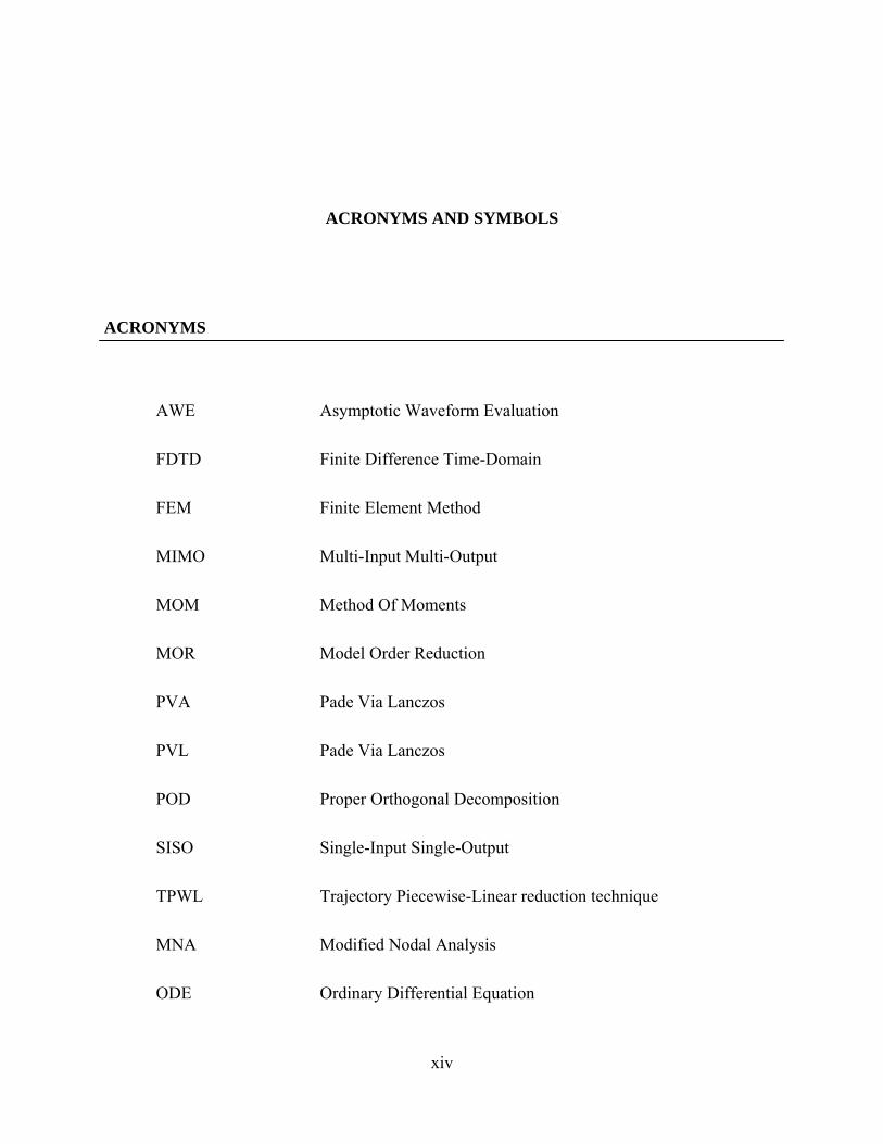
ACRONYMS
AWE Asymptotic Waveform Evaluation
FDTD Finite Difference Time-Domain
FEM Finite Element Method
MIMO Multi-Input Multi-Output
MOM Method Of Moments
MOR Model Order Reduction
PVA Pade Via Lanczos
PVL Pade Via Lanczos
POD Proper Orthogonal Decomposition
SISO Single-Input Single-Output
TPWL Trajectory Piecewise-Linear reduction technique
MNA Modified Nodal Analysis
ODE Ordinary Differential Equation

xv
KCL Kirchoff’s Current Law
KVL Kirchoff’s Voltage Law
SYMBOLS
eigenvalues
eigenvalue matrix
set of real numbers
Krylov subspace
),,( diag diagonal matrix from scalars ,,
),,( baspan spanning space of vectors ,,ba
mxnA matrix A of size m-by-n
*A conjugate of matrix A
TA transpose of matrix A
1A inverse of matrix A

xvi
ACKNOWLEDGMENTS
First of all, I would like to thank my doctoral advisor Prof. Steven P. Levitan for his continuous
support and guidance throughout this research. I am very grateful of his continuous
encouragement and patience through the good and bad times. I would also like to thank my co-
advisor Prof. Donald Chiarulli for his support and helpful insides during these years.
My thanks to my dissertation committee members: Prof. James T. Cain, Prof. Amro A.
El-jaroudi, and Prof. Rob Rutenbar for their willingness to evaluate and to provide inputs and
suggestions to improve and complete this dissertation.
Special thanks to my dear friends and colleges Vahan, Majd, and Chakra for their
insightful discussions related to this research, for their support and encouragement during the last
and long final days. Thanks to Sandy, Samuel, Joni and all the colleges at the University of
Pittsburgh that in any way contributed to the success of this project.
On a personal note, I would like to thank all my friends, for their friendship, support and
company that allow me to ride the difficult times and enjoy even more the happy days. A special
thanks to my friend Tibisay whose support and help made the difficult task a lot easier.
Finally, for all their unconditional love, patience, support and encouragement throughout
all these years of my absence, I would like to thank my family: my mother Carmen, my father
Isaud, my sister Elizabeth and my brother Johnny.

1
1.0 INTRODUCTION
The goal of this research is to develop a methodology for the model order reduction of large
multidimensional nonlinear systems. To address the broad range of existing nonlinear systems,
which makes the task of generalizing a reduction technique difficult, we use the concept of
transforming the nonlinear representation into an assembly of basic functions. These types of
functions have to be capable of representing a wide range of nonlinear problems and in doing so
serve as a canonical form. In this work and for this goal, we use linear functions but the method
is not limited to this single family. We now introduce the motivation behind our research.
Physical phenomena in nature are inherently non-linear. Until recently, CAD tool
developers could ignore this fact and assume that the behavior of microelectronic systems could
be accurately described by a set of multivariable linear differential equations. This was because
the degree of non-linearity for these systems has been minimal or controlled. However,
continued scaling, new technologies and aggressive mixed-signal design have forced us to
rethink this assumption. In particular, submicron effects, analog RF devices, parasitic
interactions and interconnection delays (including 2D and 3D effects) show increasingly non-
linear behaviors. Additionally, physics based models for multi-technology system and package
design (including optoelectronic, fluidic, thermal and mechanical analysis) are intrinsically non-
linear. Consequently, it is essential to have a methodology to deal with nonlinear systems of
2
high dimensionality since only such a solution will give an accurate description for near future
dense interconnections and complex RF and multi-domain mixed signals systems.
There are two current approaches to the generation of non-linear behavioral models, “ad-
hoc” and model order reduction. The first is based on calibrating preconceived analytic models
by incorporating data from low-level models or experimental data. The advantage of these
models is that they represent a designer’s mental picture of how a device or system works, and
therefore the state variables and constants in the calibrated models represent familiar physical
quantities and relationships. The problems with these methodologies come from a lack of detail
or degrees of flexibility in the model, a heavy dependency on the chosen sample set, the
dependency on the expertise of the designer, and the difficulty of generating such models for
complex or very large systems.
The second methodology, model order reduction (MOR), is based on directly reducing
the large state-space for the system model from a “low-level” analysis to an equivalent system
model with a reduced state-space. The initial large state representation is considered as a “black
box” that is replaced by an equivalent one whose internal dimensionality is drastically reduced
with almost no change to the input to output behavior. The problem with this technique is that,
through the reduction process, the model has lost the relationship between its parameters and the
fabrication or assembly process that created the original device or system. Therefore, the model
lacks utility for both the fabricator, in terms of predictive ability and the designer in terms of
optimization capability. Nevertheless, the advantage of this model is that it is independent of the
designer and chosen sample set and well suited for complex and high dimensional systems.
It is this ability of modeling large descriptions of systems that makes MOR the chosen
technique as the starting point for new research on the generation of non-linear behavioral

3
models. However, even though model order reduction has been applied with great success to
linear and “weakly non-linear” systems, its natural extension to the more general non-linear case
is still lacking. While there have been several proposed specific reduction approaches, the
challenge of a general methodology has not been met [1][2][3][4].
In spite of this limited progress, there is a clear consensus over the need for a successful
and widely applicable methodology for the reduction of large nonlinear system models. An
effective methodology for the reduction of nonlinear systems is an essential tool needed to
overcome future challenges such as the development of compact models for the next generation
of interconnections in the microelectronic industry, and the extraction of reduced models for new
devices and materials in the growing field of multi-domain, mixed signal microsystems.
For the generation of compact models for large nonlinear interconnection structures
found in the next generation of integrated circuits: The fact that, both current interconnect
parasitic effects and signal delays (which include 2D and 3D effects) have a highly nonlinear
response drives their extraction product to be a very dense nonlinear interconnection network.
Efficient reduction techniques applicable to these networks are essential for efficient and fast
simulation. Additionally, these compact models are required for the generation of predictive
models and optimization techniques for these interconnect structures. To accomplish
optimization it is necessary to have accurate and compact models so that the simulation and
analysis path in the design iteration cycle is fast and efficient.
For the extraction of compact models for new devices and materials: In the longer term
as new devices and materials are introduced into multi-domain microsystems, the ability to
perform nonlinear behavioral extraction for dense systems will provide a general methodology
for the modeling of these devices or systems. New active devices (e.g., Heterojunction bipolar

4
transistors (HBTs), Lateral double diffused MOSFETS (LDMOSTs) ), and passive devices with
highly nonlinear time dependent responses such as transmission lines and high-density
capacitors, require a path from the densely nonlinear distributed parametric mesh or node based
time/space discretization models, generated from physical device tools such as finite element
solvers, to a compact abstract model that is both accurate and efficient for use in optimization.
In order to move between these two levels of abstraction, new algorithms for nonlinear model
order reduction are necessary.
Perhaps most importantly, this methodology is needed at the system level where both
design for mixed-signal and multiple technologies must be supported. This methodology will
facilitate the extraction of compact models that are efficient and inexpensive to evaluate from the
low level abstraction of multi-domain devices or subsystems into a system level representation.
Therefore, in this work we propose a new methodology for nonlinear model order
reduction that is based on several propositions. First, we use the concept of transforming the
nonlinear representation into a composite structure of well defined basic functions. We address a
broad range of nonlinear systems through this transformation, casting them into a single
assembly of primitives than can then be used as the target for the reduction methodology.
Second, we build upon the concept of a training phase from the trajectory piece wise linear
(TPWL) methodology as a practical strategy to reduce the state exploration required for a large
nonlinear system. We improve upon this methodology in two important ways: through a new
strategy for the use of multiple projection bases in the reduction process and their coalescence
into a unified base that better captures the behavior of the overall system; and with a novel
strategy for the optimization of the state locations chosen during the training phase of the
technique. This optimization technique is based on using the Hessian of the system as an error

5
bound metric. Third and finally, we propose the use of a hierarchical approach using a block
projection strategy in order to treat the overall linear/nonlinear reduction task, which adds the
additional benefit of being able to track parameters through the process. This is fundamental for
keeping a direct relationship to design and fabrication parameters between the final compact
realization and the original physical system.
We believe that these three strategies together offer us a new perspective to face the
problem of model order reduction of nonlinear systems and the tracking or preservation of
physical parameters in the final compact model. Also, they can be further developed to serve as
a successful methodology to apply to a larger set of nonlinear families. In the following chapters
the rationale behind this methodology and the proposed steps to develop it are presented.
1.1 PROBLEM STATEMENT
The problem we address in this work is given a very large nonlinear system can we provide a
series of steps, which are not tied to the particular characteristics of the system under study that
allows us to obtain a compact state realization with a good level of accuracy between the reduced
model output and the original system response?
We attack this problem, the development of a methodology for the state reduction of very
large nonlinear dynamic systems, with the following steps:
The use of well defined primitive functions for the approximation (i.e., linear functions) for
the general nonlinear system at specific state-space locations (i.e., sampling points).
The use of training trajectories to select sample points that characterize the system being
studied. These trajectories are by themselves samples in the vast volume of the domain of
6
the nonlinear system. This also can be seen as an additional level in the sampling of the
state-space of the problem.
The assembly of the set of primitive snapshots or approximations to generate a general
representation for the original system that is valid in the explored volume of the state-space.
The use of a multi projection base methodology to reduce this assembled structure into the
desired reduced target state-space.
The optimization of the location of sampling points in the state-space that allows us to reduce
the approximation error for substituting the original system by its assembled counterpart.
The introduction of a block projection technique in the reduction process that allows us to
decompose linear and non-linear sub-blocks in the original large system description. This
can also be used for the further tracking of relevant parameters through the reduction process
itself.
The focus of the present work is to introduce a novel series of improvement on the
current strategy for model order reduction of nonlinear systems that are primarily oriented to
improve the robustness and accuracy of the resulting compact models. We expect improvement
on the evaluation speed for the new models when compared to the evaluation of the original
large system as expected because of the reduction on the dimensionality of the system. We do
not expect improvement over the associated training phase related to this type of techniques. The
opposite is expected, since we are adding additional processing to account for the new robustness
and accuracy goals.

7
1.2 STATEMENT OF WORK
The problem of the state reduction of very large nonlinear dynamic systems has a series of
particularities that needs to be addressed in order to devise a successful solution. The first
paramount difficulty associated with this problem is the large variability of the types of target
systems. Contrary to a linear system, a general nonlinear system can exhibit a large difference in
terms of structure (i.e., connectivity) and nonlinear function types in its components. To try to
generate a general strategy to reduce such a large set of possible input candidates appears to be
an intractable proposition. A solution to this difficulty and the one we follow in this work is to
transform the original system into a collection of basic functions that approximate the behavior
of the original nonlinear system by regions in its state-space domain. When the responses from
these individual functions are merged we then have a solution that approximates with good
accuracy the complexity of the original system.
Since we already have a solid understanding of MOR for linear systems, it is a good idea
to use linear approximations as the basic functions in the previous process. The original problem
now has been transformed to a known functional structure from which we can derive a sequence
of steps that allows us to reduce its large state-space size.
We are faced now with a second difficulty in this development. Because of this generic
transformation we are forced to sample the state-space of the original system to capture
representative snapshots. These snapshots are equivalent to the basic models we have selected
and in fact are adjusted to match the behavior of the system as close as possible at their
respective sampling locations. However, the difficulty now is how and where to sample the
original state-space of the system under reduction. The sampling of the space is a demanding
task in its own right since the state-size, for the type of systems we are interested in, is very

8
large. Since to effectively map the volume of space for any system under study would require an
impractically large number of samples, we have chosen to follow an economical alternative, a
trajectory based strategy. Trajectory based sampling is a method that minimizes the sampling
requirement for a problem of this type. It is based in the premise that the system operates under
a series of known families of inputs and that following the state behavior of the system under
these excitations give us preferred locations in its state-space where to sample and in so doing
captures well the behavior of the system.
We then face our third difficulty in the path to a reduction methodology for large
nonlinear dynamic systems. Since we now have a collection of linear approximations for regions
in the state-space of the original we can use well established linear MOR techniques to reduce
the state-space of these sub-models into a smaller size representation. The question at this point
is how to derive a projection base that allows this reduction to take place. We could use the
linear approximation gathered from one of these sampling points to obtain the desired projection
base. This is a simple approach but clearly susceptible to a larger error in the generated reduced
model since it does not use the rest of the linear approximations in the set for the base generation
process. Because of this, we choose to develop a mechanism that uses the information of each
sampling point to generate corresponding projection bases. Consequently, in our development
path we have to design a strategy to merge the resulting set of projection bases into a
consolidated base that best captures the behavior of the original nonlinear system.
The fourth and final difficulty that we need to overcome for the development of the
nonlinear model order reduction technique is the merging of this collection of individual
representations of the system into a single assembled model. A general mathematical operator
can be associated with this process, a spatial function that distributes the contribution of each

9
sub-model into the final arrangement. We can also see this figure as an “envelope” that
modulates each individual contribution. The definition of this function however will affect the
behavior of the methodology as a whole. In order to choose this function we are presented with
the task of trading off complexity and consequently computational cost in the final model against
degree of accuracy and independency.
This merging function can also be understood as a proportional operator, also known as a
weight function [3] that defines the relative contribution that each sub model has in the final
assembly for each location in the sate-space. We can assign conditions to the overall behavior of
this function, such as: a) its norm always being one (i.e., 1w ) to avoid any additional scaling
for the final model, b) its behavior to be dependent on the state-space location which allows
fitting the original state-space using the collection of snapshots, c) to be highly selective when
approaching the location where the snapshots are sampled and to decrease rapidly to zero when
moving further from these locations. In the selection of the nature of this weight function we
have to decide its number of degrees of freedom which in turn affects its flexibility and accuracy.
In one extreme of the range of choices, we can have a simple switching scalar function that only
has one degree of freedom for the adjustment of the contribution of the individual sub-models.
And at the opposite extreme, we can select the weight to be a full matrix function representation
that affects each individual state contribution in the final assembly and in doing so offers the
largest degree of freedom for the matching process.

10
In the course of this dissertation we chose to use a scalar function for its simplicity.
However there are limitations in the resulting model as a consequence of using such an
economical strategy. The generated compact model is very dependent on the selected sampling
points used in the method, and more specifically in how far from these locations the system
operates.
In order to reduce this dependency, we perform an optimization on the selection of those
locations in the state-space where a glimpse of the behavior of the original system is sampled. A
good placement of those points allows us to better capture the behavior of the original system
and equally important to minimize the error associated with evaluations outside these locations.
In summary to achieve the previous goals, we perform the following tasks:
Development of a test environment in MATLAB [5]: This tool is required to
provide a common platform for the implementation of the different model order
reduction strategies that we use in this research. Additionally, this environment
also allows us to perform comparisons between these different extraction,
modeling and simulation techniques within a common modeling and simulation
tool.
This environment consists of the following modules:
o Linear MOR algorithms: Krylov based projection algorithms (Arnoldi (single
and double sided), Lanczos, State transformation balancing algorithms.
o Different training, evaluation and optimization modules used in this
dissertation.
o SPICE [6] netlist parser/translator and a MATLAB non-linear analog solver
(i.e., circuit solver) module.

11
Use of a Block projection methodology: Use of block projection for the
separation of linear and nonlinear subsections in the representation to further
simplify the subsequent reduction process. The goal of this task is to develop a
successful methodology for the partition/reduction of a complex system. The
model reduction process is considered as a hierarchical task where blocks are
identified and separated according to their behavior. Linear, weakly nonlinear,
moderate nonlinear and highly nonlinear sections are the target for this
classification task. Each section can then be targeted with the most suitable
technique for its modeling.
Decomposition and projection extraction of Sub-regions: Divide the state-
space domain of the nonlinear system into sub-regions close to each other and
approximate those using basic functions (e.g., linear approximations). The aim of
this task is to generate a standard representation from any general given nonlinear
system. Once this approximation is generated, use well known linear MOR
techniques (e.g., Krylov based methods, Truncation methods) to obtain a suitable
projection base to translate it to a reduced state-space representation.
Generation and coalescence of linear projection bases (Multi-projection
support for the extraction methodology): First, to use the multiple sampling
points in the state-space of the function under study to not only generate the linear
approximations to use in the reduction process but also to generate an equal
number of projection bases for the reduction mechanism itself. And, second, to
develop a method to consolidate the whole set of projection bases into a single
unified one that is more suitable for the region under study. The fundamental idea

12
for this task is to acknowledge that to generate a suitable projection base for the
whole domain under consideration requires more information that what can be
gathered from a single state-space location.
Hessian based optimization strategy for the sampling of the state-space: To
use the second order terms of the nonlinear behavior of the system (Hessian) to
evaluate the range for the linear approximation at any sampling location. The
goal of this task is to use the Hessian information to produce a metric for the
region that can be used in the estimation for the size of the linear representation.
To develop an optimization algorithm for the selection of sampling locations in
any trajectory used when generating the set of linear approximation models.
Performance evaluation (Multi-projection strategy): Through a set of test
cases, evaluate the efficacy of the use of a multi-projection strategy over a single
projection base generated from a single point in the state-space of the original
large nonlinear system.
Performance evaluation (Sampling space optimization): Through a set of test
cases, evaluate the efficacy of the use of the strategy for the optimization on the
selection of state-space locations for the linear approximations on the original
nonlinear system, as opposed to the use of the simpler strategy of a homogenous
sampling in the original state-space.
13
1.3 CONTRIBUTIONS
The major contributions of this dissertation are the followings:
To our knowledge we are the first to introduce the use of the Hessian of the nonlinear
function in a nonlinear large system representation as the basis to generate a metric that can
be used to judge the quality of the linearity in a quasi-linear region of those found in a
trajectory based piece-wise linear methodology. We avoid the computational cost of finding
the exact maximum value of the Hessian and its location in the vicinity of the linearization
point establishing instead an approximated value at this location. The metric is based on the
use of the Lagrange remainder of the second order for the Taylor series expansion of the
multidimensional function at the sampling location. The importance of this proposal is the
use of this metric for the optimization of the location of sampling points in the chosen
trajectories and as a consequence in the volume of space under study.
We use multiple projection bases in the reduction process together with the optimization of
the location of samples in the state-space of the nonlinear system under study to improve the
accuracy of the generated model while conserving its size to a minimum. Tiwary and
Rutenbar [43] also use the concept of multi-projection base for the improvement in the model
generation. However, the mayor difference in both approaches is the progressive merging of
individual bases in our case and the use of an orthogonalization algorithm to accomplish this.
Our approach iteratively update the aggregated projection base each time a new projection
base is generated using an orthogonalization procedure based on the Gram-Schmidt algorithm,
while Tiwary adds each base as a whole leaving the pruning as the last stage of the process.
While the final result of both methods is equivalent we believe that an iterative approach is
more efficient in terms of memory use while paying a small cost per orthogonalization per

14
region. This cost is compensated by the low cost of the truncation of the final projection
base. Progressive orthogonalization offers a combined projection base that is already free of
common subspaces. Consequently the cost of the final SVD operation for the truncation to
the desired size is smaller. It is important to remark that Tiwary’s approach does not grow
alarmingly in size since he is already selecting a small number of bases for the merging using
his nearest neighbor-clustering approach.
We introduce the concept of hierarchical reduction for a large nonlinear system realization to
divide and simplify the overall reduction process. The use of a block projection approach
allows us to identify linear and nonlinear blocks in the original representation that can be
treated separately to reduce the overall effort in the reduction task.
Over the past years several groups have developed and enhanced the idea of using
trajectory piecewise linear models for non-linear model order reduction. Our contributions and
their relation to the work of M. Rewienski et al, J. Roychowdhury et al, and S. K. Tiwary and R.
A. Rutenbar, are summarized in Table 1 and in the conclusions of this document. There is a
clear similarity with the work of S. K. Tiwary but our strategies although when offering similar
solutions are obtained by different approaches.
Table 1. Contributions and relationhip to significant research in the area.
Order of
sub-models
Sub-region volume Hierarchy Support Multiple
Projection Bases
M. Rewienski et al
[3][42]
Linear Fixed No No
J. Roychowdhury
et al [4][41][59]
High Order
(+2nd / 3rd)
Fixed No No

15
Table 1 (continued).
S. K. Tiwary,
R. A. Rutenbar
[43][44][45]
Linear Computed using nearest
neighbor approach
(Training and Evaluation
Phase)
Support limited
hierarchy
Yes
J. A. Martinez Linear Computed using the
Hessian (Training Phase)
- Chapter 7 -
Theoretical proposal
- Chapter 3 -
Yes
- Chapter 6 -
1.4 DISSERTATION ROAD MAP
This document is organized as follows:
In Chapter 2, we discuss the background of this research. We start with a definition of
model order reduction for linear systems, and then we follow with a classification of the main
strategies available in this field. We then introduce the more challenging, and main thrust of this
research, the model order reduction of nonlinear dynamic systems. We present a review of the
ideas currently used for the reduction of large nonlinear system representations and the
difficulties and limitations found in each one of these techniques. In doing so, we establish the
need for improvement upon the current alternatives for the generation of compact models for
large nonlinear dynamic systems.
In Chapter 3, we propose to use a hierarchical approach for the reduction process of a
very large nonlinear system. We introduce the use of block projection instead of a single
projection base for the model order reduction of general systems. We discuss how to separate

16
the state-space representation for the large system under study by blocks and develop the
corresponding modification to the reduction process. Specifically, we explore the advantage that
a projection base defined as a diagonal sub-block projection base [7] offers to the model order
reduction task. We show how using a block projection base strategy gives us the ability of
detection of linear/nonlinear sections in the original system representation that can then be
separately treated simplifying the overall reduction task.
Because of the need for a common simulation platform with which to compare our
reduction methodology with current comparable techniques, in Chapter 4, we introduce the
development of our MATLAB based analog solver platform. This set of programs that allow the
simulation of compatible circuit descriptions (i.e., SPICE netlists) was developed to support our
research in nonlinear circuit simulation and model order reduction. In this chapter we discuss in
detail the simulation strategy used in its development, as well as its more important components.
We follow with a performance comparison between both this novel platform and a commercial
well known circuit solver, HSPICE [8]. We conclude the chapter with a summary of the
advantages, the limitations and future improvements for this simulation tool.
In Chapter 5, we present the trajectory based piecewise-linear technique for the model
order reduction of large nonlinear systems. Because we are using this technique as the starting
point to develop a more optimal strategy to deal with this type of problem, we dedicate this
chapter to a detailed analysis of this method. After initially describing the algorithm and the
details surrounding the ensemble final model, we then present its advantages and limitations with
the help of a series of test cases.
In Chapter 6, we show that in order to improve the accuracy of nonlinear model order
reduction a multi-projection base approach needs to be used. We initiate the discussion with a

17
description of the sources of error in a piece-wise based reduction methodology. We then show
how when using a single base generated from a single state point the accuracy of the generated
model is impaired when the nonlinearities are contained in a larger state-space than the one
defined by that single base. We propose an algorithm to merge the information from multiple
projection bases obtained from an equal number of sampling points to generate a more suitable
base for the volume of space considered. We follow with the description of the strategy to
accommodate this extended projection base into the piecewise-linear method. We conclude the
chapter with a series of test cases where we show how the new multi-projection approach allows
us to better capture the overall behavior of the original system through a smaller error in the final
output.
In Chapter 7, we introduce a novel mechanism to generate a linearization metric that can
be used to optimize the location of the states for the linear approximations in the reduction
process. We discuss how the performance of the resulting compact model is highly dependent
on the behavior of the weight function (simple scalar envelope function), and that this function in
turn is very sensitive to the state-space location for the linear approximations. As an
improvement over a simple ad-hoc region size definition, we introduce a radius metric that is
derived from error bound estimation at the linearization location. This error bound is defined
using the Hessian of the system and considers the remainder of the linear series approximating
the nonlinear function. We finish the chapter with test cases where we show how the new
strategy gives a reduced number of required regions for the same error limit when compared to
the fixed radius approach.
In Chapter 8, we present our conclusions and finally in Chapter 9 we discuss some ideas
for extending the scope of this research.

18
2.0 MODEL ORDER REDUCTION
Initially in this chapter, we present a brief summary on the history of the development of the
model order reduction field from its initial work, born from control theory, up to the current
efforts for application in nonlinear dynamic systems. After the definition of model order
reduction we then follow with a classification of the main strategies used for model order
reduction (MOR) of linear dynamic systems. We then address the current and more challenging
problem of the model order reduction of nonlinear systems. We follow with a review of the
important ideas currently being used to deal with the general problem of model reduction for
nonlinear systems. We show the difficulties found when trying to reduce the order of these types
of problems and give references to some of the representative research in this area. Note that
Appendix A gives more detail on some background concepts.
2.1 A BRIEF HISTORY
The idea of the reduction of a system model to a lower dimensional equivalent has been of much
interest to the area of control for a long time. Research was particularly intense during the 60s
and 70s as pointed out by Genesio and Milanese in [9]. Until that time the interest had been
focused in answering the question of what the minimal size representation of a linear dynamic
system was, and in controlling complex systems through the use of simple linear models. It is

19
not a coincidence that this period also corresponds to a wider use of digital computers for the
simulation of previously prohibitively complex dynamic systems. These new tools offered the
designers the capacity to simulate very large models resulting from both very complex dynamic
systems and distributed systems. Additionally, they also motivated the research community to
investigate the possibility of widening the applicability of these tools to an even larger set of
problems through the use of model order reduction.
Kalman [10][11], also during this period, helped the rebirth of the use of state-space
representation for the control of dynamic systems. He proposed an answer to the minimal size
representation problem for a linear dynamic system through the use of the state-space
formulation and the concepts of observability and controllability subspaces. Through his
research the stability and control of dynamic systems became easier and clearer tasks.
During the following decade formal strategies for the reduction of the state-space
representation were introduced. The reduction process was then proposed as the truncation of a
state-space model representation using the relative importance of the states in the input-output
behavior. Moore [12][13] proposed the idea of a balanced realization as a preliminary step
before the reduction process. A balanced realization was presented as the linear transformation
that eliminates any scaling effects over the internal representation of a state-space model.
Kabamba [14] improved over the balanced realization concept with the introduction of balanced
gains instead of the principal values used by Moore, for weighting the contribution of the states
to the input-output behavior. Additional research into the balancing strategy followed as
described for example in [15] - [18].
In the meantime, the problem of truncating the state-space realization was also
considered as equivalent to the geometrical projection of the original formulation to a reduced

20
state-space. This strategy allows us to translate the reduction process into the extraction of an
effective projection base. It was discovered that an approximation to the solution of a dynamic
linear system is contained in a Krylov subspace that can be readily defined from the original
state-space representation of the system. This was relevant since Krylov subspaces [Appendix
A.3] had been widely used as an alternative solution for the eigenvalue problem of linear systems
together with iteration methods to derive the associated orthogonal bases for these geometrical
subspaces. Efficient techniques that are based on iteratively finding the projection base for the
associated Krylov subspaces of a dynamic linear system were developed soon after. Methods
based on one side-Krylov subspace (input or output Krylov subspace) [19][20][21] or two-sided
Krylov subspace (both Krylov subspaces) [22] - [25] have been considered together with
efficient iterative procedures for orthogonal base generation such as Lanczos [26], Arnoldi [27]
and Padé [28] techniques.
The idea of MOR was present but suitable applications that demanded the development
of effective techniques to accomplish it were not in place. This soon changed; during the 90’s
when the demands for simulation of very large interconnection electrical networks in VLSI
became the test bed for model order reduction techniques. Algorithms such as PVL [29][30],
and PRIMA [31] proved to be very efficient for the simulation of such a large systems. They
showed that very large interconnection problems can be reduced to more manageable compact
representations which allow the designer to simulate the whole network in a more reasonable
time. This was important because traditional simulators such as SPICE [32] could not deal with
such large problems without incurring extremely long simulation times or impractical memory
requirements.

21
After the success of PRIMA for this type of application, efficient MOR techniques have
been developed and applied in many different areas to deal with the simulation of large
dimensional problems [33][34][35]. This continuous and evolutionary process has been the
source of additional requirements which have brought refinements and improvements over the
original methods. Currently, model order reduction for linear systems is a very mature area of
research with very efficient algorithms. One of the main focuses of research in this field is to
find algorithms that can offer error bounds for the reduced model without sacrificing the
performance already obtained by the established techniques. Stability is also not guaranteed in
any of the current Krylov based algorithms, consequently an additional research push is to merge
the stable simple truncation of state technique with the efficient computational Krylov subspace
based technique.
A different type of problem also has recently raised considerable interest in the research
community. It is well known that most of the systems in nature are of nonlinear behavior;
however, until now a linear model approximation was an acceptable solution. However, the
increased nonlinear effects observed in recent observed large systems have changed this
situation. These include nonlinear effects in the interconnection networks and new switching
devices of current VLSI designs, in the lumped parameter description of micro-electro-
mechanical devices (MEMs), and the ones found in the space-time discretization for new multi
domain mixed signal device or systems. A new group of algorithms that are adaptations from
the linear MOR field have been considered to cope with this kind of problem. Some of these
methods [36] - [40] are based on the Proper Orthogonal Decomposition (POD) technique, which
is the generalization of the idea of finding a suitable projection base, V, for the reduced model of
nonlinear systems as done in the linear case. This projection, V, is generated or estimated
22
through information from data samples of the state-space of the original model or through linear
approximations. Another group of techniques is based on linearizing part of the state-space of
the solution and in doing so applying the well known and efficient set of tools for MOR from the
linear area [3][4][41][42][43][44][45]. We should also mention a small group of specific
solutions that are very successful for nonlinear systems of limited size and constrained behaviors
[43][47][48].
2.2 MODEL ORDER REDUCTION
MOR is a field derived from system control theory that concentrates in the study of those
dynamic systems with a very large dimensionality whose space or time dependent behavior can
be described by a compact realization that still conserves the desired input-output port behavior.
One of the main goals in this area of research is to develop methodologies that allow the designer
to identify and to generate those compact models that mimic the behavior of the very large or
infinite state-size system problems. Small realizations allow more efficient computational
simulations of very complex systems and are the basis for optimization techniques and control
algorithms on those kinds of problems.
The following is a list of the desirable characteristics for a MOR algorithm:
Good Accuracy: The most important aspect of any MOR methodology is that the
final compact model can offer minimal error on the behavior of the input-output
relations of interest from the original system.
User independency: It is highly desirable that the final algorithm offers minimal
user intervention when generating the compact realization for a specific system.

23
The algorithm should be highly independent of the specific characteristics of any
system that is intended to work on.
System properties preservation: For many types of problems, it is desirable that
the final realization conserves specific properties or parameters of the original
system.
Computational efficiency: There are two aspects on how computationally efficient
a MOR technique is. The first is how computationally costly is the generation of
the compact realization. In this metric the user should decide if the cost of the
generation is justified over the costly evaluation of the very large initial system.
The second is how computationally efficient is the evaluation of the compact
realization when compared to the original.
There are two well defined sub areas in this field, MOR of linear and MOR of nonlinear
systems. As expected, linear MOR is a well known and developed area of knowledge that is
itself used as the basis for research in the newer and still developing field of nonlinear MOR.
We start with a description of the linear case and follow with an analysis of the current state of
development for the nonlinear area.
2.3 MOR OF LINEAR SYSTEMS
The transformation of a very large size linear model to a compact model representation has been
accomplished through many different approaches. However, we present in this section four of
the most widely used and successful methodologies developed in this area, namely:

24
Polynomial approximations of the transfer function (e.g., moment matching
techniques),
Truncation of the state-space representation approach
Subspace projection techniques, and
Proper Orthogonal decomposition
A very wide spectrum of methods has been developed that are based on these basic
approaches or in their combination.
In order to get the best results, the recent techniques being developed in the area of linear
MOR have contributions from several of these main thrusts to overcome any of their individual
weakness and add to their combined advantages.
2.3.1 Polynomial Approximations of the Transfer Function/ Explicit Moment Matching
techniques
Polynomial approximation is performed on the transfer function representation of the system
usually in the frequency domain. The basic principle in this approach is to approximate the
system using the truncated power series expansion of its transfer function. Let us consider a
linear state-space representation of a dynamic system with u as the input vector, y as the output
vector, and x as the state vector for the system:
,
,
xCy
BuAxxT
(2-1)
Where A is the transformation matrix of the system, B is the input connectivity matrix
and C is the output connectivity for the system model.
The transfer function of the system expressed in the frequency domain is given by:

25
,)( 1bAsICsH T (2-2)
Where I is an identity matrix, and the output of the system is then given by,
),()()( susHsy
We can expand )(sH around 0s and obtain an infinite power series of this transfer
function as:
,..,..,)(110
211
i
m
iT
m
T
m
TT sBACsBACBACBAsICsHi
The coefficients mi associated with the polynomial terms, also known as moments of the
system are the main target for the polynomial approximation techniques. A reduced
representation for the system consists of several of these terms with a suitable approximation for
the coefficients. Padé approximation [28], the Routh algorithm [49], and stability equation based
techniques belong to this category of MOR. The expansion can be performed at any other point
besides s=0, and at several points as well, in order to better match certain system behaviors. As
an example, if the expansion occurs at s then the matching of coefficients corresponds to
the process of matching the Markov parameters between the system to the model and the reduced
representation [50]. A very good agreement with the behavior at high frequencies of the system
is achieved with this approach but with a poor performance at low frequency operations.
The main advantages of this approach are that it is relatively computationally inexpensive
in its operation and that the resulting model has a good match for system behavior at the
expansion point. The main disadvantages however are that it is difficult to guarantee stability for
the resulting model, to estimate the error bound on the compact model, and it is difficult to apply
to multi-input, multi-output (MIMO) systems. This method does not guarantee passivity (a
system is passive if it only consumes energy, there is no mathematical instability that allows the

26
energy in the system to grow without bounds) for the resulting compact model even when
starting from a passive original system. This creates a potential source of instability in the final
compact model. Several modifications have been developed to preserve passivity through the
reduction process and also to allow it to be successfully applied to MIMO systems [29][31].
2.3.2 State Truncation Approach
Truncation methods are based on state-space realizations of the system. The idea is the
systematic reduction of the state-space to only include the subspace that is primarily responsible
for the observable input-output behavior of the original system. The main advantages of these
techniques are that they are inherently stable and easy to scale and apply to MIMO systems, and
that they have defined error bounds. Additionally, because they keep the zeros and poles
associated with the remaining states, they give us a good match for the input-output behavior of
the system through the whole frequency spectrum. The difficulties associated with these
methods are that they are relatively more computationally demanding, they preserve input-output
behaviors but do not guarantee to capture all the system behaviors, and that the tracking of
parameters from the original system is difficult to achieve.
We already mentioned that the Kalman proposal of a controllability and observability
subspace allows for a clear representation of the process of a truncated state-representation as a
model order reduction technique. Let us now use the description of the reduction process as
presented by Lohman [51] to clarify this concept.
We consider a large linear state-space representation of a dynamic system as in (A-1) and
proceed to apply a transformation such that the resulting representation of the system is diagonal.
The required transformation can be achieved if the transfer matrix for the system, A, can be

27
expressed through an eigenvalue decomposition as 1 VVA , where is the diagonal matrix
of Eigenvalues of A and V represents the matrix of the corresponding eigenvectors. Using V as
the orthogonal base for the linear transformation of the system gives us the desired conversion.
We show this in the following steps:
,
,
,
, 1111
xCy
BuVxVxV
xCy
BuxVVxTT
(2-3)
And using the transformation of states xVz 1 we obtain:
,ˆ
,ˆ
,
,1
zCy
uBzz
VzCy
BuVzzTT
(2-4)
The diagonalized state-space representation for the model is:
,ˆˆ
,ˆ
ˆ
1
1
1111
n
n
nnnn
z
z
CCy
u
B
B
z
z
z
z
(2-5)

28
Figure 1. Block diagram of system model This new representation in (2-5) is a set of linearly independent equations that add
together to produce the observed behavior of the system. Consequently, if we put this equation
set in a block representation as shown in Figure 1, we can identify graphically the association to
the Kalman’s concepts of controllability and observability for this system.
From this block diagram we can see how, if the system has a set of states jz , whose
associated TjC are nulls, they do not affect the output, y , of the system. This implies that these
states are unobservable. Additionally, if there is a set of states kz , whose associated kB are null,
this set of states are isolated from the outside of the system. This implies that these states are
uncontrollable because the input )(tu has no effect over them. This set is, according to Kalman,
a potential source of instability for the model since any initial condition or noise reflected on

29
these states could drive the system to an unstable or unpredictable response. These two sets can
be taken out of the final model without affecting its input-output behavior. This resulting model
corresponds to the minimal state-space realization proposed by Kalman.
This presentation also gives us the basis for a further reduction of the system. If we
identify those states of the representation in Figure 1 with an overall small value for B , and TC ;
we can conclude that their contributions are weak compared to the rest. Consequently, their
elimination should have a minimal effect on the overall behavior of the model. This elimination
of weak states is what constitutes the basis for the truncation mechanism for the model order
reduction technique. It is essential to remark that this reduction procedure by truncation gives us
an approximated model for the system instead of a minimal realization which is an exact model.
It is at this point that we can see that a correct assessment of the effect of the states over
the input-output behavior is important for achieving a proper truncation of the system. The
balancing methods proposed by Moore and other researchers aim to transform this realization to
reflect the importance of the states in terms of the impact over the behavior (see [12][13] for a
detailed explanation of Moore’s balancing method). These methods in general can be
understood as balancing the system in terms of the amount of energy required to drive it to a
specific state against the effect of a certain value of energy associated with that state has on the
output of the system.
Even though the previous description covers the essence of the technique, practical
considerations need to be addressed. It is computationally inefficient if we have to completely
solve an eigenvalue problem as a first step in the model order reduction method. Using a method
such as Gaussian elimination or a similar technique to achieve eigenvalue decomposition would
clearly be a very costly (i.e., )( 3nO ) for very large representations. However, if we have a

30
closer look at the problem statement we can see that what is really required is to obtain that
reduced set of “important” Eigenvalues of the balanced realization. Any additional computation
for weak components is unnecessary and a waste. An additional aspect that is useful to see is
that the whole process can also be seen as a projection to a lower state-space dimension. Instead
of the cropping of states, we can describe the process as the projection of the initial realization to
a lower dimensional state-space where the solution is contained. This is the basis for the next
very useful contribution to the model order reduction technique, the use of orthogonal
projections based on Krylov subspace theory.
2.3.3 Subspace Projection techniques
A different but related way to understand the process of model order reduction of a system is to
consider the concept of projection into a subspace of a smaller size [53]. The idea behind the
method is to project the system under study from its original state-space NN into a subspace
KS of lower dimensionality (i.e., K<<N) while maintaining its behavior from the point of
view of the output nodes of interest.
This concept has a clear geometrical interpretation, as the associated name implies. Each
of these subspaces can be completely represented by rectangular matrices that can be understood
as composed of columns that correspond to the bases for the respective subspaces. However, as
known from linear analysis, any base characterizing a subspace is not unique since there are
infinite numbers of equivalent bases that can completely define such a subspace. Nevertheless,
any one of these bases is equivalent in terms of this characterization.
Let us again consider the general state representation for a linear system:
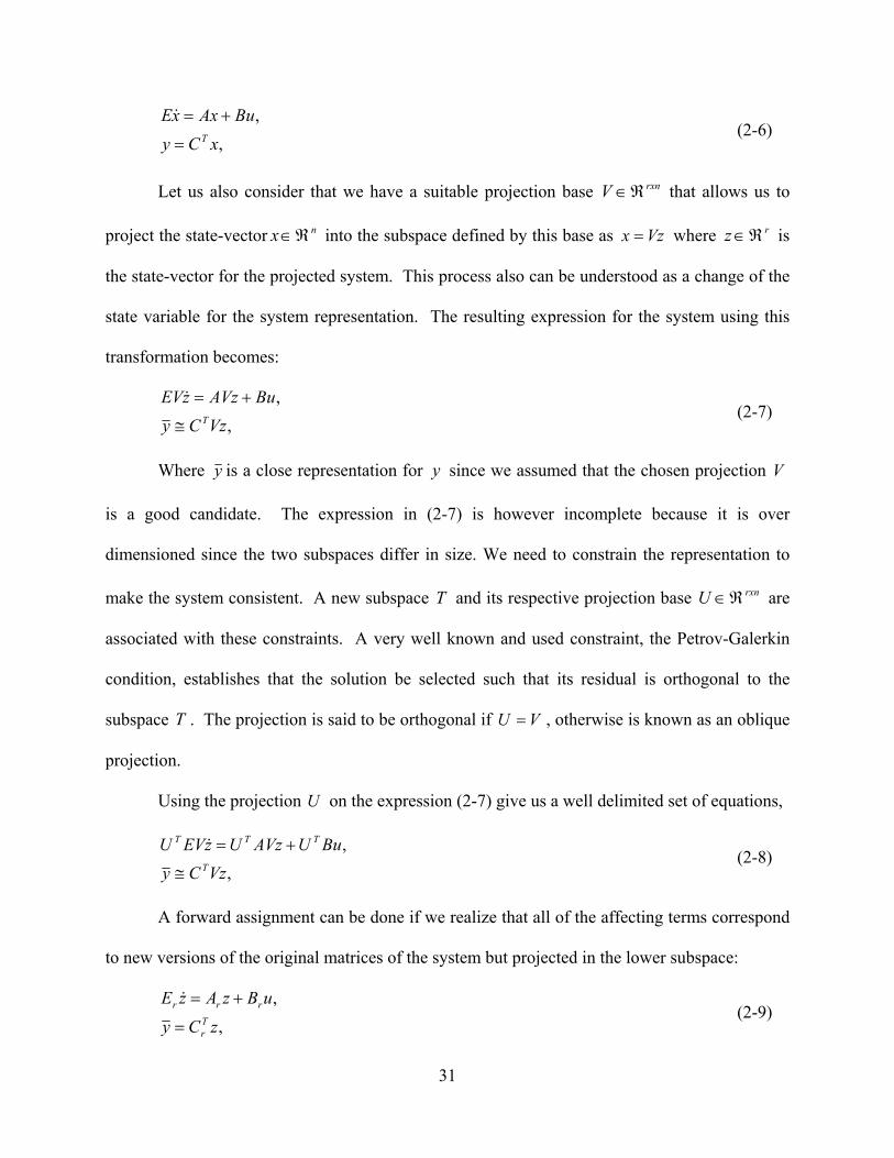
31
,
,
xCy
BuAxxET
(2-6)
Let us also consider that we have a suitable projection base rxnV that allows us to
project the state-vector nx into the subspace defined by this base as Vzx where rz is
the state-vector for the projected system. This process also can be understood as a change of the
state variable for the system representation. The resulting expression for the system using this
transformation becomes:
,
,
VzCy
BuAVzzEVT
(2-7)
Where y is a close representation for y since we assumed that the chosen projection V
is a good candidate. The expression in (2-7) is however incomplete because it is over
dimensioned since the two subspaces differ in size. We need to constrain the representation to
make the system consistent. A new subspace T and its respective projection base rxnU are
associated with these constraints. A very well known and used constraint, the Petrov-Galerkin
condition, establishes that the solution be selected such that its residual is orthogonal to the
subspace T . The projection is said to be orthogonal if VU , otherwise is known as an oblique
projection.
Using the projection U on the expression (2-7) give us a well delimited set of equations,
,
,
VzCy
BuUAVzUzEVUT
TTT
(2-8)
A forward assignment can be done if we realize that all of the affecting terms correspond
to new versions of the original matrices of the system but projected in the lower subspace:
,
,
zCy
uBzAzETr
rrr
(2-9)
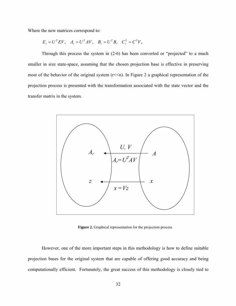
32
Where the new matrices correspond to:
, , , , VCCBUBAVUAEVUE TTr
Tr
Tr
Tr
Through this process the system in (2-6) has been converted or “projected” to a much
smaller in size state-space, assuming that the chosen projection base is effective in preserving
most of the behavior of the original system (r<<n). In Figure 2 a graphical representation of the
projection process is presented with the transformation associated with the state vector and the
transfer matrix in the system.
Figure 2. Graphical representation for the projection process However, one of the more important steps in this methodology is how to define suitable
projection bases for the original system that are capable of offering good accuracy and being
computationally efficient. Fortunately, the great success of this methodology is closely tied to
x
U, V
x =Vz z
A Ar Ar=UTAV

33
the theory of Krylov subspaces. The recent progress of projection based model order reduction
for large linear systems came from the development of efficient projection algorithms based on
Krylov subspaces. Krylov subspace theory establishes that the solution of a linear system of the
form in (2-1), (2-6) resides in a subspace of order q which also corresponds to the rank of A. This
subspace can be very small compared to the original size of the problem and more importantly
researchers have developed computationally efficient iterative methods that allow for the
definition of the associated subspace, such as the ARNOLDI algorithm [54] and the LANCZOS
projection technique [55]. For more information on these algorithms the reader is referred to
Appendix A.5.
2.3.4 Proper Orthogonal Decomposition
Proper Orthogonal Decomposition (POD) is a powerful technique developed in the field of data
analysis that captures the behavior of large dimensional systems into a small size description.
This method is also known as Principal Component Analysis (PCA), the Karhumen-Loéve
Decomposition or the Single Value Decomposition (SVD) method [56].
The method has been used widely in control and estimation applications because of its
ability to generate accurate descriptions for very complex systems with a small number of
elements. The method attempts to extract characteristic information from a data set as a group of
uncorrelated POD models or parameters. For this extraction an orthogonalization procedure is
used as the filtering tool. One of the advantages of this methodology is that it is capable of
working from either an experimental set of data from a physical model or a state representation
of it.
34
Let us consider that we want to approximate the function ),( txf in an interval of interest
X by the following series of terms:
N
kk xgtatxf )()(),( (2-10)
We are considering the approximation as a series of products of separated functions for t
and x dependencies. It is reasonable to assume that we can increase the number of terms in the
series, N , to obtain any desired level of accuracy for the approximation. x is usually considered
to be a state-space dependency while t is the time dependency for the function. While there is no
mathematical consideration to distinguish between these variables it is common to separate the
expression in these two flavors mostly because of the physical significance of the nature of the
system.
There are several criteria use to select the set of functions kxg )( chosen for the
approximation in (10), orthogonality being one the most widely chosen. According to this
restriction the set of functions kxg )( obey:
ji
jidgg
X
ji 0
1)()( (2-11)
Accordingly the terms kta )( in (2-10) can now easily be obtained since they are only
dependent on the corresponding kxg )( term as:
dgtfta k
X
k )(),()( (2-12)
However, there are still many orthogonal sets of functions that can be used for the
formulation in (2-10). Depending on this selection the preceding process carries on a well
known approximation, such as a Fourier series (sines and cosines), Fourier-Legendre series
(Legendre polynomials), Chebyshev series (Chebyshev polynomials), etc. We can set a further
35
restriction for the selection of this set; we can ask which set offers the best approximation in
terms of least square error against the original function for each specific number of terms. This
set of orthogonal functions is what is called the Proper Orthogonal nodes for the set and the
resulting approximation is known as Proper Orthogonal Decomposition (POD) of ),( txf [57].
One of the more powerful features of this method is the ability to work with a set of
snapshots of the function under study if the analytical expression ),( txf is not available, in what
is called the method of snapshots.
Given a set of snapshots in time or observations },1:)({ XxNixF i on some
physical system of explicit or unknown function ),( txf over the domain X , we want to obtain
an approximation )(~
xF with the least square error to the snapshot set )(xF .
Using the definition for the inner product as X
FdFFF ~,
~, the approximated function
)(~
xF can be defined using a series as presented in (2-10):
N
kk FaF~
(2-11)
Where the desired coefficients ka are to minimize the cost function R
N FF
FF
NR ~
,~,
~1
2
(2-12)
Through some mathematical manipulation shown in [78] this translates to the eigenvalue
problem:
YUY
Where TNaaaY ],..,,[ 21 is the vector of unknown coefficients ka , , and U is the
correlation matrix for the snapshot set given by:

36
jiij FFN
U ,1
(2-13)
The solution of this eigenvalue problem give us a set of N eigenvectors, kY , for each
corresponding eigenvalue, k . The Eigenvalues are sorted in descending order
n 21 , and so the eigenvectors are arranged. This set can be truncated to obtain a set
of the desired orthonormal Eigenfunctions F~
:
N
kKkK
Nkk FaFFaF N K ,
~ , ,
~ 11 (2-14)
After reviewing some of the current techniques for linear MOR, we turn now to nonlinear
systems.
2.4 MODEL ORDER REDUCTION OF NONLINEAR SYSTEMS
Model order reduction of nonlinear systems is the natural consequence of model order reduction
in the linear realm. However, the extension of concepts from that area of research has not been
easy or successful. The difficulties for this task are a result of the complexity and variety of
nonlinear systems when compared with the clearly defined structure of linear systems, and the
lack of a general and solid theory for formal minimization and state-space projection as is
present in the linear counterpart. Nevertheless, extensive research is underway for establishing a
formal base for these concepts in the nonlinear field. In the meantime, the main strategies
currently used to address this problem are based on linear approximations in order to apply solid
concepts borrowed from the linear model order reduction field.

37
The main approaches used for the modeling of nonlinear systems can be summarized as:
Linearization methods, Quadratic methods, Piecewise trajectory based methods and Proper
Orthogonal Decomposition techniques. We now proceed to discuss each in turn.
2.4.1 Linearization Methods
Linearization methods are the earliest and most straightforward approach to model nonlinear
systems. Their strategy is based on linearizing the system around a point in its state-space and
applying well known linear model order reduction techniques to the resulting approximated
representation. In this approach the system is expanded around an operative state-space value
using, for example, a multidimensional Taylor series expansion technique. After this, the
resulting sum of infinite terms is truncated to only the first order term or linear component. The
result of this is the Jacobian of the nonlinear multi-dimension function of the system used as a
linear model approximation. Let us show this process using the following nonlinear system
representation, as a generalization of the linear case above:
,
)(
xCy
Bu,xfxT
(2-15)
A very wide range of non-linear problems can be mapped to a representation like this.
Where nx is the state vector, ku is the input vector, my is the output vector,
nxkB is the input connectivity matrix, mxnTC is the output scanning matrix, and
nf represents a nonlinear set of functions. If a multidimensional Taylor series expansion
around 0x is applied for this system it gives us:
38
,
,..,)()()0( 321
xCy
Bu,xxxWxxWxWfxT
(2-16)
The infinite series of terms in (2-16) exactly match the system in (2-15) around the
expansion point. The typical Jacobian matrix nxnW 1 represents the first order contributions
on the state variables, 2
2nxnW is a tensor that represents the second order contributions and in
general knxn
kW corresponds to a tensor with the thk order effect contributions.
In the linearization method the system is approximated as a truncated expansion series
with only the first order contributions or linear effects. From the model in (2-15) this
corresponds to:
,
)0( 1
xCy
Bu,xWfxT
(2-17)
From this point, the designer can obtain the compact model of the system using any of
the well known linear model order reduction techniques. As an example an Arnoldi algorithm
over the Krylov input subspace BWKq ,11 gives us a projection base nxrV such that Vzx
can be used to achieve the reduction. As previously established the resulting order r is much
smaller than the original state-space size, n.
,~
~~)0(
~
,
)0( 11
111
zCy
u,BzWfz
VzCy
Bu,VVzWVfVzTT
(2-18)
2.4.2 Quadratic Methods
Quadratic methods are an improvement over the previous approach where the second order term
of the expansion in (2-16) is also included for the state-space approximation of the nonlinear

39
system. The purpose of this addition is to improve the accuracy of the representation and extend
its validity over a larger state-space. With this consideration the system in (2-15) is
approximated as:
,
)()0( 21
xCy
Bu,xxWxWfxT
(2-19)
This expression is known as a second order or a quadratic state-space representation. We
now have the tensor 2
2nxnW to account for second order effects. From this result a similar
procedure to the previous case is used. A simple approach is to consider the Krylov subspaces
defined by the linear part of the representation, ignoring the second order term, to obtain the
desired projection base nxrV . Then the resulting projection Vzx is used over the whole
expression in (2-19) as:
,
))(()0( 12
11
11
VzCy
Bu,VzzVVWVVzWVfVzT
,~
~)(
~~)0(
~21
zCy
u,BzzWzWfzT
(2-20)
Where we used the projection to the new state-space, linear algebra manipulation and
substituted the matrices for their reduced counterparts.
There are also specially designed methods for the extraction of the projection base V in
(2-19), known as quadratic projection methods [7][19][52]. They are based on considering the
effect of the linear and second order component for the definition of the Krylov subspace and the
generation of the corresponding orthogonal vector base.
Both of the previous methodologies are limited to a good match of the system only in the
neighborhood of the expansion point. The success of both techniques is strongly dependent on
the closeness to a linear or quadratic representation of the original system. This fact makes such

40
techniques well suited for weakly nonlinear systems [19][58][59][60] but a very poor solution
for moderate to highly nonlinear problems.
2.4.3 Piecewise Linear Model Order Reduction
The piecewise trajectory technique was introduced to improve upon the limitations of the
previous linearization methodologies for generating a compact model from a large nonlinear
state-space by Rewiensky and White in [3][42]. In this approach, the approximated model is
built using multiple expansion points in the state-space of the original state-space model. The
compact model is created through the merging of linear approximations of the original system
over this set of expansion points.
The selected expansion points for the reduction are generated following a “training
trajectory” through the state-space of the original system. The authors are consequently, using
these specific training trajectories, avoiding the difficulty of dealing with the large volume of the
original state-space realization. Under this strategy, the proposed solution is specially tailored
for the volume of the state-space that is in the neighborhood of the selected training trajectory.
The justification for this approach, as suggested by the authors, is that the model functionality is
confined and accordingly conditioned by the input set commonly employed in the system.
Efficient model order reduction techniques can then be applied on these linear
realizations so a proper projection base can be found. For the joining of this linear set, a weight
function is used that depends on the Euclidian distance between the current state and the
expansion state point for each individual linear sub-model. The effect of this weight function is
a swift transition between sub models and to weigh the contributions of neighbor subsystems to
an evaluation point.
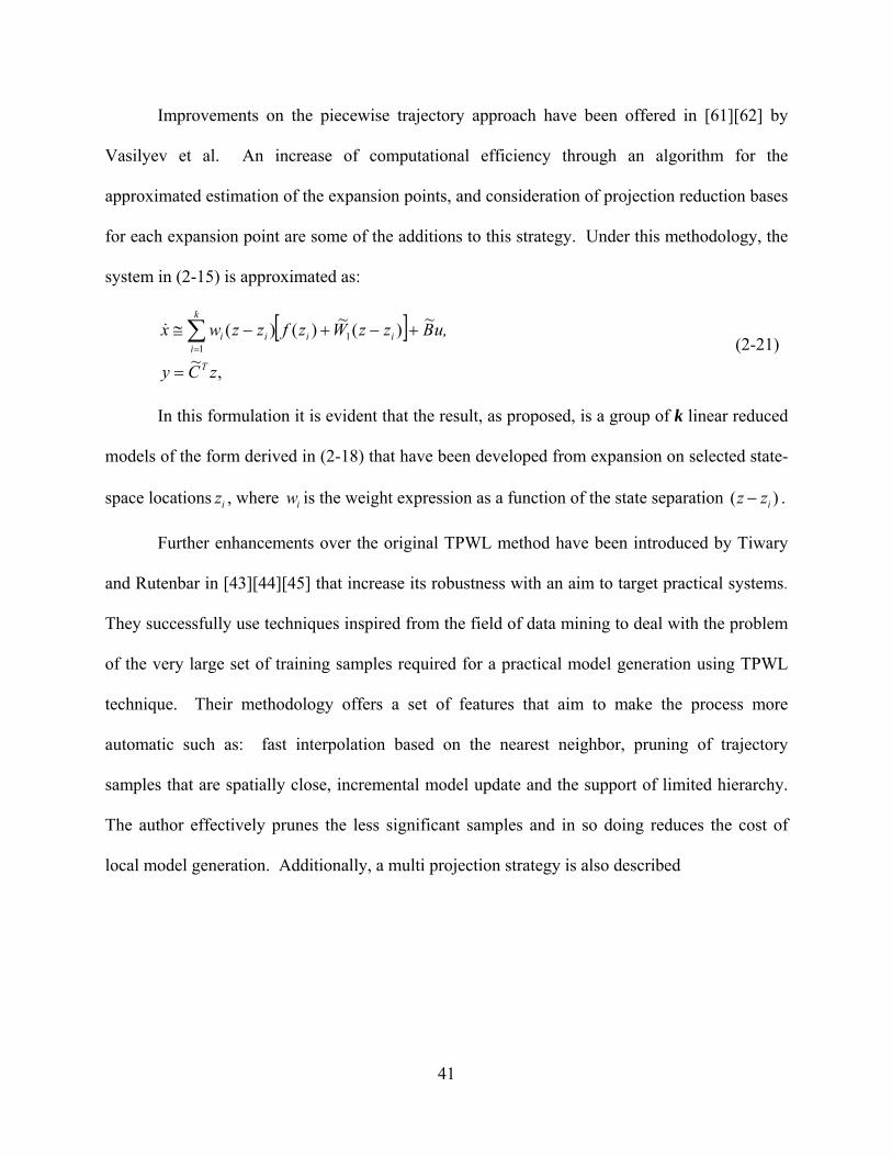
41
Improvements on the piecewise trajectory approach have been offered in [61][62] by
Vasilyev et al. An increase of computational efficiency through an algorithm for the
approximated estimation of the expansion points, and consideration of projection reduction bases
for each expansion point are some of the additions to this strategy. Under this methodology, the
system in (2-15) is approximated as:
,
~
~)(
~)()( 1
1
zCy
u,BzzWzfzzwx
T
ii
k
iii
(2-21)
In this formulation it is evident that the result, as proposed, is a group of k linear reduced
models of the form derived in (2-18) that have been developed from expansion on selected state-
space locations iz , where iw is the weight expression as a function of the state separation )( izz .
Further enhancements over the original TPWL method have been introduced by Tiwary
and Rutenbar in [43][44][45] that increase its robustness with an aim to target practical systems.
They successfully use techniques inspired from the field of data mining to deal with the problem
of the very large set of training samples required for a practical model generation using TPWL
technique. Their methodology offers a set of features that aim to make the process more
automatic such as: fast interpolation based on the nearest neighbor, pruning of trajectory
samples that are spatially close, incremental model update and the support of limited hierarchy.
The author effectively prunes the less significant samples and in so doing reduces the cost of
local model generation. Additionally, a multi projection strategy is also described

42
2.4.4 High order Piecewise Model Order Reduction
A variation of the previous technique has been offered by Roychowdhoury in [4], in which the
author achieved an improvement on the accuracy of the sub-models through the use of a
quadratic or higher polynomial term. Roychowdhoury proposed that while the global effect is
properly captured by the piecewise trajectory approach, the local effect can be more efficiently
represented by a higher polynomial reduction model.
The main difficulty faced by this or similar techniques is the dependence on the selected
state-space trajectory of the system and consequently in the training input set used for the
generation of the reduced model. The relationship of input to state-transformation is unknown
for the system without a wide exploration of the state-space. Consequently, the selection of the
training set does not give us a clear understanding of the related state trajectories. Similar input
training sets could produce widely diverging state-trajectories. Consequently, the validity or
applicability of the model is highly dependent on the correct selection of the training set.
Interesting or hidden behaviors might be not captured by the final model because a selected input
training does not cover that sub-volume of the state-space. It is this dependency that restricts this
method from being considered as a general solution for the problem of nonlinear model order
reduction of large systems.
2.4.5 Proper Orthogonal Decomposition
Proper Orthogonal Decomposition (POD) [63][64] has received renewed attention recently as an
alternative technique to use for model order reduction of nonlinear systems. The method has

43
been used widely in control and estimation applications because of its ability to generate accurate
descriptions for very complex systems with a small number of elements.
In these algorithms the definition of a small set of POD models can be seen as a parallel
idea to the definition of a small space for a linear reduction system. Consequently, the method
can be understood as the process of defining a suitable projection V that captures a
characterization of the data samples of the problem. The projection V is generated or estimated
through information from data samples of the state-space of the original model or through linear
approximations. If these data samples match a linear system the POD elements correspond to
static values or parameters. For a general behavior data set, the POD elements correspond to a
general orthogonal basis. The main differences between this methodology and the previous
approaches are that the resulting model is not restricted to a limited volume of the original
problem and not restricted to be a linear or lower order approximation of it. The sampling data is
not limited to belong to clusters or to follow a particular driven trajectory in the state-space of
the original model. The POD models are also not limited to be linear or quadratic functions but
any function that captures the behavior of the selected set of data samples.
A group of variations of this method have been presented [36][37][38][39][40] for the
reduction of specific nonlinear problems. The main difficulties in this methodology are the
selection from the data set or state-space of the snapshots (i.e., set of samples) that characterize
the behavior of the system, and determining the reduced set of POD elements that closely match
those behaviors. The selection of snapshots requires knowledge of the final solution of the
system which is not always available or practical to generate.
After having explored the current state of research in this area we follow in the next
chapter with a presentation of the major ideas behind our proposed research.

44
2.5 SUMMARY
In this chapter we have introduced the reader to the field of model order reduction for very large
dynamic systems. This field has reached a level of maturity suitable for its current use as a
major tool in the design and analysis on such diverse areas such as Aeronautic control, VLSI and
Micromechanical technology to name a few. A brief history of the accelerated development and
principal research contributions on this field of knowledge were presented together with a
reference to its current challenges.
We then introduced a formal definition of the main goal in this field together with the
series of characteristic that are desirable in a technique of MOR and introduced the classification
of the field into two mayor subfields, MOR of large linear systems and its nonlinear counterpart.
For the linear MOR area, we presented the problems in the field and described the most
widely used and successful techniques that have been developed and implemented. Krylov
based MOR techniques were discussed as offering several key advantages that have made them
the preferred techniques for MOR.
For the MOR of large nonlinear systems, we have also introduced the reader to the nature
of the problem being addressed and reviewed several of the current efforts to develop a
successful methodology. In the following chapters we describe one of these techniques in detail,
the Trajectory piecewise-Linear (TPWL) technique for model order reduction of nonlinear
devices [3]. We also present our implementation of this methodology with a description of its
virtues and limitations. This technique is used as the starting point for our development of an
improved methodology to deal with nonlinear systems.

45
3.0 BLOCK PROJECTION TECHNIQUE FOR MODEL ORDER REDUCTION
In this chapter we explore the use of a block projection technique to improve the efficiency of
the linear MOR methodology. We propose the use of the separation of the state-space
representation for the large system under study by blocks, and develop the corresponding
modification to the reduction by projection. Specifically, we explore the advantage that a
projection base defined as a diagonal sub-block projection base [7] offers to the model order
reduction task. We show below that this technique gives us the ability to partition the system
into specific sub blocks, each one affected by its separated sub projection base. Through this
ability to partition dynamic systems during the reduction projection process we can consider the
modeling task as a hierarchical process. Additionally, we prove that this block projection
technique can also be used in the model order reduction process of nonlinear systems. The
nonlinear model order reduction task can then be related to any additional linear or nonlinear
interaction taking place in the system. We first look at the use of block projection instead of a
single projection base for linear model order reduction of linear systems. Finally, we extend
these results to the more general case of a nonlinear representation.

46
3.1 LINEAR SYSTEM REDUCTION USING BLOCK PROJECTION
A block partition [7] offers us the ability of partitioning a specific linear state-space model in
terms of its state representation. This ability of doing selective partitioning is useful because it
allows us to separate the linear and nonlinear subsections of a state-space representation and, it
gives us the ability to selectively separate a subset of original parameters in the original model
representation so it can be subsequently tracked through the reduction process.
Let us describe the block projection reduction applied to a general linear state-space
representation. Given a general state representation of a linear system:
),()(
),()()(
txCty
tButAxtxT
where
lmn
nxlnxmnxn
yux
CBA
,,
,,, (3-1)
Assuming that instead of a single orthogonal projection base for the reduction process we
use the following partition projection:
,0
0
2
1
2
1
2
1
z
z
V
V
x
xx where
2121
21
21
21
,
,,
,,
,,
21
21
2211
qqqnnn
xx
zz
VV
nn
xqnxqn
(3-2)
Let us remark that using this projection base we are transforming the representation from
nx to a reduced state-space qz where nq (as previously presented in 2.3.3).
With this projection into (3-1) and using block forms of ,, BA and C of the proper size, this
system can be expressed as:
),(0
0
0
0
0
0
2
1
2
1
2
1
2
1
2221
1211
2
1
2
1 tuB
B
V
V
z
z
V
V
AA
AA
V
V
z
zTT

47
,0
0
2
1
2
121
z
z
V
VCCy TT where
,,
,,2212
2111
2221
1211
xnnxnn
xnnxnn
AA
AA
,,
,,21
21
21
21
xlnxln
xmnxmn
CC
BB
(3-3)
where we have used the orthogonal property of the selected base, IVV T .
Finally, the system in (3-3) can also be expressed in the following form after some linear
algebra manipulations:
zCCy
tuB
Bz
AA
AAz
TT21
2
1
2221
1211
~~
),(~0
0~
~~
~~
where
222111
222111
222222121221
21211211111
~,
~,
~,
~,
~,
~,
~,
~
VCCVCC
BVBBVB
VAVAVAVA
VAVAVAVA
TTTT
TT
TT
TT
(3-4)
As seen above, we have done a selective partition of the original state-space
representation using the block projection technique. An interesting case to consider is when one
of the projections is a unitary base. This gives us a partition where we can preserve a subset of
the original state in the final reduced model. This particular application can be used for the
tracking of desired physical parameters from the original system to the reduced final model. As
we show next, the same idea can be generalized to nonlinear systems as well.
3.2 SUB-BLOCK NONLINEAR SYSTEM REDUCTION USING BLOCK
PROJECTION
To understand the more general case of applying block projection for model reduction over a
general nonlinear representation, we first consider the case where there is a clearly defined
nonlinear sub system in the model representation. The subsystem operates in a subspace of the

48
state-space representation. We want to verify that it is possible to use a projection base for
reducing the linear section of the representation and additionally be able to define the effect of
this projection on the nonlinear section.
Given a state representation of a system which has a nonlinear subsection on a subset of
the state-space:
),()(
),())(()()( 21
txCty
tButxftAxtxT
where
21
21
,
,,,
,,
,)(,
21
21
nnn
yu
xxx
CB
fA
lm
nnn
lxnxnxm
nxnnxn
(3-5)
Let us first convert the given system to a block representation in terms of the size of the
subspaces defined by x1 and x2:
),()(
)(
2
1
2
1
2221
1211
2
1 tuB
B
x
x
fA
fA
x
x
,2
121
x
xCCy TT where
,)(,
,)(,2212
2111
2221
1211
xnnxnn
xnnxnn
fA
fA
,,
,,21
21
21
21
xlnxln
xmnxmn
CC
BB
(3-6)
where, again, we are using a block representation of A, B and C with the proper sizing, as
used in (3-3). Let us again use the orthogonal partition projection in (3-2), for the order
reduction process:
),(0
0
0
0
)(
)(
0
0
2
1
2
1
22
11
2221
1211
2
1
2
1 tuB
B
V
V
zV
z
I
V
fA
fA
V
V
z
zTT
,0
0
2
1
2
121
z
z
V
VCCy TT (3-7)

49
where again we are using the orthogonality of the selected base, IVV T .
After some manipulation (3-7) can be transformed into a more compact model
representation:
,~~
),(~0
0~
)(~~
)(~~
21
2
1
22
1
2221
1211
zCCy
tuB
B
zV
z
fA
fAz
where
222111
222111
22222
121221
12112
111111
~ ,
~ ,
~ ,
~),()(
~ ,
~),()(
~ ,
~
VCCVCC
BVBBVB
fVf
VAVA
fVf
VAVA
TTTT
TT
T
T
T
T
(3-8)
It is important to see that the problem has been reduced by block projection to a partition
formulation with separate linear and nonlinear components. The result is a separated by block
representation that has also being reduced in state-size ( qz ).
Finally, if we choose the nonlinear projection to be the unitary base, the model is
transformed to:
,222 , xzIV
),(0
0~
)(~
)(~~
2
1
2
1
2221
1211
2
1 tuB
B
x
z
fA
fA
x
z
,
~
2
121
x
zCCy TT (3-9)
In (3-9), we have achieved our goal of reducing the linear portion while preserving the
nonlinear characteristics of the system. An important aspect of this development is that if the
nonlinear subsection is affected by any projection, this projection should be considered for the
other subsections of the system as seen in (3-8).
These results allow us to directly apply model order reduction to this type of hybrid
linear/nonlinear system. This clearly will be efficient in situations where 21 nn so an
integrated non-linear model order reduction can be obtained.

50
Of course, the challenge is the model order reduction of the general nonlinear case.
However, the previous conclusions and possibilities offered by the block partition technique are
directly applicable to a general model order reduction process. What this technique offers is the
ability to take a general system and, by selecting the proper projection block, reduce and
partition sub sections of it. It also shows us that special care has to be taken when dealing with a
system with linear and nonlinear combinations. We have to apply a nonlinear reduction
technique to the nonlinear section but any equivalent projection base developed for this process
( 2V in the previous development) needs to be also applied to the rest of the system as described
in (3-8). This is because the sections are not completely independent; the nonlinear state subset
and the linear set influence each other.
In chapter 6, we present a possible approach to reduce this nonlinear sub block of the
system.
3.3 SUMMARY
In this chapter we have shown how the block projection techniques give us the ability to treat a
complex and large dynamic system in a hierarchical way for the task of its model order
reduction. This technique allows us to perform the simultaneous order reduction and partitioning
of the dynamic system under test. There are additional advantages of its use such as the capacity
of isolating a set of parameters from the original state-representation from the effect of the MOR
process (e.g., allowing the tracking of physical parameters) We also established that, knowing an
extraction path for the non-linear component, we can apply block projection for model order
reduction to a general nonlinear system.

51
4.0 DEVELOPMENT OF A MATLAB BASED ANALOG SOLVER FOR USE AS
TEST BED OF MOR METHODOLOGIES
In this chapter we present the development of our MATLAB platform for the simulation of novel
devices in the context of traditional CMOS circuit netlists. This environment also provides a
means to perform comparisons between different extraction, modeling and simulation techniques
within a common modeling and simulation tool.
We first present our motivation and strategy for the development of the simulator, and
then we show the performance of our simulation tool compared to a well known circuit simulator
HSPICE. We show that simulation results are almost indistinguishable in terms of accuracy
when the mathematical models chosen to represent the physical components in both tools are the
same. Also, when compared in terms of the number of iterations per evaluation, both tools give
similar cost per evaluation. However, it is understood that the computational speed of a
simulation platform developed on top of a MATLAB framework is not comparable to an
optimized commercial tool. Nevertheless, the intended goal for this platform is to provide a
single comparative and stable environment for the different algorithms developed during this
work and to be available to other researchers who are doing similar work using the MATLAB
environment.

52
4.1 MOTIVATION
Increased design productivity is predicated on the development of new CAD tools for exploring
larger design spaces more quickly and more thoroughly than can be achieved with current
techniques. This design exploration is most often accomplished in a design-simulation-analysis
loop which is limited by both the speed and quality of the simulation tools used for analysis and
evaluation. For many designs, well known models and design abstractions allow for the accurate
analysis of both analog and digital circuits using circuit simulation tools such as SPICE. It is
often possible to use higher level abstractions and faster simulators for timing and power
estimations of large digital systems.
However, for new technologies, the simulation of the behavior of new devices and
components are often ad-hoc and incompatible with traditional simulation environments. Device
model development is often done using physics based models implemented directly in a
programming language or with mathematical modeling tools such as MATLAB. Therefore, it is
challenging to model systems composed of novel devices together with conventional devices
(e.g., CMOS) in a single evaluation environment. There is an increasing need to evaluate these
new devices, which are often based on new technologies, or hybrids of existing technologies, and
to simulate circuits and systems that include both new and traditional devices.
Not only do we need to provide a methodology for these multi-technology simulations,
but also, there is a need to evaluate new simulation techniques and new model extraction and
abstraction techniques, such as reduced-order modeling. It is easier to evaluate the quality of
these new modeling methodologies and simulation algorithms if they can be easily integrated
into an environment where standard circuit netlists can be parsed and simulation results can be
compared to existing tools. However, integrating these new ideas into open source versions of

53
SPICE [6] or other simulators is a time consuming and needlessly frustrating exercise. On the
other hand, MATLAB gives a very flexible environment and is currently in widespread use for
model development. To our knowledge, there are currently no non-linear circuit solvers, or
analog solvers, built into MATLAB and no way to parse circuit netlists (e.g., SPICE “decks”)
into the MATLAB environment.
To address both needs, we have developed a flexible MATLAB simulation platform that
supports SPICE netlists in conjunction with abstract device models for compatible simulations as
well as enabling comparisons between different extractions, modeling and simulation techniques
with a common baseline environment.
Our work, to date, has resulted in a Perl [65] based SPICE netlist parser/translator and a
Matlab non-linear circuit solver module. The SPICE parser module generates MATLAB script
files from typical netlist files and supports such useful SPICE constructs as sub-circuits, input
sources, and transistor model parameters. These scripts are then used as input to our MATLAB
non-linear circuit solver. The solver is based on the same non-linear iterative stamp, or template,
based technique developed for SPICE, and currently supports adaptive time-stepping, initial
condition convergence, as well as backwards Euler and trapezoidal integration methods. Generic
SPICE options are provided such as RELTOL, ABSTOL, VNTOL, LVLTIM, and GMIN. The
solver currently has hard coded models for resistors, inductors, capacitors, diodes and default
MOS transistors. Support is also provided for custom MOS models as well as generic multi-port
non-linear electronic devices.
Given that the solver is written in MATLAB, the environment provides the ability to
dump and load the internal data structures, and thus generate snapshots of the system state, for
interaction with external circuit analysis and optimization tools.

54
It is important to note that these tools are in no way replacements for SPICE or any other
simulation tool developed primarily for fast simulation of analog circuits. Rather, these
programs were developed to support our own research in non-linear circuit simulation and model
order reduction. Along the way, we realized it would be useful to be able to use SPICE netlists
for our tests. Therefore, we have written these support tools to translate a simple SPICE netlists
into MATLAB scripts files along with some supporting MATLAB function files and a wrapper
function. The wrapper function ties these all together and invokes the non-linear circuit solver.
In the following sections we describe in detail the simulation strategy used in the
development of this simulation platform as well as its more important components. Finally, we
present several tests where we compare the performance of this tool against a commercial SPICE
implementation, HSPICE [8]. We conclude the chapter mentioning the advantages in this
developed tool as well as its current limitations and suggest some future improvements.
4.2 SIMULATION STRATEGY
A typical analog simulator can be characterized by the way it performs three major tasks: nodal
analysis, linearization of nonlinear elements, and integration of time dependent components, as it
moves the system under study through the evaluation cycle. We discuss each of these tasks in
turn:
Nodal Analysis - The first task of any analog solver is to convert the system under
analysis into a mathematical linear representation that accurately captures the behavior of the
system at each evaluation time. A general mathematical representation allows one to formulate a

55
methodology for the evaluation of such a system that is independent of its structure and
components.
A dynamic linear time invariant system can be completely defined as a set of ordinary
differential equations (ODEs) in terms of a set of variables that constitutes what is referred as the
system state. This ODE set relates the state of the system to its inputs using an invariant
parametric matrix description. Any variable of interest from the system can then be derived
using a set of algebraic expressions in terms of this defined system state.
This matrix representation carries information about the system, where its specific values
are dependent on the individual elements, but the matrix structure itself only depends on the
structure of the system. The formal justification of the previous claim can be found in bond
graph theory [66]. This theory allows one to study the behavior of a dynamic system as a state
defined system. The future behavior of this system is completely deterministic if an initial state
at a previous time is known, and the history of the inputs to the system since that moment is
completely specified.
For the purpose of the explanation of the evaluation method that is presented in the
following sections we introduce the matrix representation for an electrical system as an example
[A-1]:

56
u yS
MRB
x
Figure 3. Dynamic system representation
,BuRxxM (4-1)
DuxEy T (4-2)
As shown in Figure 3, the system S is defined as characterized by the matrix set M, R,
and B1, the state-vector x, and the vector u that represents the excitation to the system (4-1). The
desired system outputs, y vector, are in general derived from this representation through an
algebraic expression (4-2). This expression maps the state vector x, and inputs to the system u
through the incidences matrices TE and D respectively. From this representation, any linear
1 The M,R,B notation is commonly used when describing MNA representations in the electrical field, this description is, however, also assigned the sequence E,A,B in the control and mathematics fields when referring to the matrix representation for a 1st order linear system. Even when both are equivalent, we use the latter convention through the rest of this document.

57
analysis method can be applied to derive the current state of the system and, in doing so,
encapsulate the response in physically identifiable variables (e.g., current, voltage, force).
In the majority of analog solvers in use, a variation of nodal analysis is used to
mathematically describe the system [67]. Under this methodology, characteristic points in the
circuit which correspond to concentrated values of a variable of interest are identified and
principles of conservation of flow and potential are then used to describe the governing
relationships (e.g., electrical current and voltage, and corresponding Kirchoff’s laws for
electrical circuits).
For our current analog solver implementation, we have chosen Modified Nodal Analysis
(MNA) to create a mathematical representation for electrical netlists, as shown in Figure 4. In
this expression, M corresponds to the memory matrix of the system, also called the reactance
matrix, R is the conductance matrix, x is the vector of state variables, B and E are
connectivity matrices, u is the excitation vector, and the y is the vector containing the desired
output variables from the system. The reader is provided with a more detailed description of this
representation in Appendix B.
The linear elements can be directly mapped to this representation, but the non-linear
elements need to first undergo a further transformation.

58
Modified Nodal Representation:M x = - R x + B u; y = E T x+Du
M Storage element R Conductance
i x State variables B, E Connectivity matrices
u Excitation vector y Evaluation vector. C
L
0
0
C T
L T
M
M T Template from a bounded non-linear element (i.e., nodes <N)
nodes= N
D Incidence matrix.
.
Figure 4. Modified Nodal Analysis Representation
Linearization of nonlinear elements - Nonlinear devices in the system are replaced by their
equivalent stamps (also called templates) which are simply the local nodal matrix representation
of the linearized element at the current operating point. Because of the nonlinear behavior of
these elements, an iteration loop is required to reach a convergence state. This involves finding a
state for the current evaluation time that satisfies all the elements in the system.
Integration of time dependent components - For time dependent elements in the system, such as
energy storage devices (e.g., capacitors and inductors) an integration loop is required. A
linearization of these elements is provided by using one of several integration techniques and the
error in their application is estimated with an associated error bound algorithm. The

59
convergence state reached in the inner loop is validated to meet the error tolerance that has been
chosen for the evaluation.
These three core tasks are used repeatedly by the simulator for the accurate estimation of
the time evaluation of a given system. The minimal configuration for an analog solver involves
two major stages: Initial operating (OP) point evaluation (also known as DC evaluation) and
transient evaluation. The OP stage allows the solver to estimate a valid operative point for the
system under analysis given the available information for the initial state. In the other hand, the
transient evaluation allows the solver to progress in time from the current valid state, given the
inputs to the system. Since the transient stage requires a valid state for the system to start from,
the OP stage is the first step in any solver operation. In the next section we discuss each of these
stages in detail.
4.3 OPERATING POINT EVALUATION (DC EVALUATION)
The first major stage for an analog solver is to find a valid operation point for the system at the
requested initial time given any available information on the initial state. Several strategies have
been developed and implemented through the commercial development of practical circuit
solvers [8]. It is important to remark that in many situations, this is a crucial step and sometimes
the most difficult bottleneck in the simulation. For this project, we have chosen to implement
several strategies to provide a highly reliable IO step that is also efficient in terms of
computation time. The proposed algorithm uses three techniques:
The use of GMIN (minimum conductance) as a leakage parameter for the initial estimation of
an operating point. These temporary leakage conductances are added between each node and

60
the reference node (e.g., GND). This strategy forces all loops in the electrical circuit to be
closed loops, avoiding the possible situation of unconnected (i.e., floating) nodes, which are
commonly found when using nonlinear circuit elements during IO evaluation. Floating
nodes can cause an ill-conditioned transfer matrix for the system, and in doing so create
convergence problems.
A “cold evaluation” attempt as the first pass. This is a simple evaluation of the circuit that
does not consider temporal dependencies (derivatives). Therefore, the storage elements in
the circuit (C, L) are considered in steady state. Capacitors act as voltage sources and
inductors as current sources with initial values corresponding to the initial condition (IC)
values specified in the netlist or zero if not specified.
A source stepping algorithm as the second pass. This is a stable and reliable algorithm where
the circuit is considered initially not energized. Then, a progressive step by step increase in
the value of each independent power source is performed. The final value for each stepping
progression corresponds to the DC value for the considered source in the netlist. When all of
the sources are completely stepped, a final operating point has been reached. While this is
not necessarily the only possible operating point, the main goal of the algorithm is to produce
a valid one.
Even though we are reaching for a DC operating point, we must consider the time
dependencies in the system. Therefore, this algorithm tries to achieve convergence in the
nonlinear evaluation by first using a simple time stepping algorithm, and in case of failure,
reinitiates the evaluation using local truncation based error (LTE) strategy for the dynamic
control of timesteps [68]. This combination has proven to be both reliable and efficient.

61
4.4 TRANSIENT EVALUATION
In this stage, the goal is to successively move the system through the given time period,
generating its proper response within the allowed error tolerance at each advancing timestep.
Starting from the operating point found in the previous stage, an iterative process is initiated to
obtain the desired response.
The main core of this stage is the convergence algorithm, which for this implementation
is based in an iterative gradient method. The main kernel of this algorithm is shown in Figure 5.
We now briefly describe each step:
1. The validation of the state information, operating point and input and output requirements
is performed.
2. The generation of stamps (i.e., templates) for storage elements is accomplished in this
step. These stamps correspond to the linearization of each element based on the chosen
integration method.
3. This the top of the main convergence loop. Nonlinear elements stamps are created
corresponding to the current operating point (i.e., at time tn). This is followed by an
integration of these linear stamps into the MNA representation of the circuit.
4. A linear solution is generated corresponding to the predicted new operating point, for
timestep tn+1.
5. A check for convergence is performed.
6. If the solution is not convergent, the timestep is decreased based on the chosen dynamic
control algorithm.
7. A dynamic control of the time step is performed. During this step, even if the system is
convergent, the evaluation point can be rejected based on an unacceptable estimated
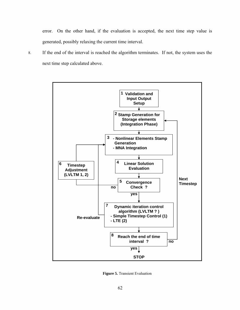
62
error. On the other hand, if the evaluation is accepted, the next time step value is
generated, possibly relaxing the current time interval.
8. If the end of the interval is reached the algorithm terminates. If not, the system uses the
next time step calculated above.
STOP
Next Timestep
Timestep Adjustment (LVLTM 1, 2)
Re-evaluate
- Nonlinear Elements Stamp Generation
- MNA Integration
Validation and Input Output
Setup
Linear Solution Evaluation
Stamp Generation for Storage elements
(Integration Phase)
1
2
3
6
Dynamic iteration control algorithm (LVLTM ? )
- Simple Timestep Control (1) - LTE (2)
no
Convergence Check ? no
yes
Reach the end of time interval ?
yes
4
5
7
8
Figure 5. Transient Evaluation

63
4.5 SPICE PARSER
Starting with the goal to simulate a variety of CMOS circuits without having to hand code
netlists into MATLAB data structures, we developed a netlist parser. A Perl function parses a
SPICE netlist and generates a set of MATLAB functions callable by the solver, as well as a
MATLAB script file representing the netlist itself. The parser is modular and could be used in
other environments to parse SPICE files into other formats.
The parser is based on the Perl package, Parse::RecDescent [69]. The basic operation of
the parser is simply to take the element statements of the netlist (e.g., R, L C, and M) and convert
them into function calls to add elements into the internal simulator data structures. Element
parameters with SPICE scale modifiers (e.g., K, U, P, and F) are supported. For MOS transistors,
length, width, and model names are also understood. Voltage and current sources are mapped to
MATLAB functions which return voltage or current values as a function of time. MOS “model
cards” are converted into MATLAB functions which are invoked by the simulator to set device
parameters prior to circuit evaluation.
To make it easier to parse common circuits, file includes, line continuations and
comments are supported. Nested sub-circuits are also supported, which is probably the most
useful aspect of the whole parser.
The output of the parser is a MATLAB script file. This script file is then evaluated by
the solver resulting in the creation of the internal data structures it requires for the simulation,
including the netlist structures for the voltage and current sources.
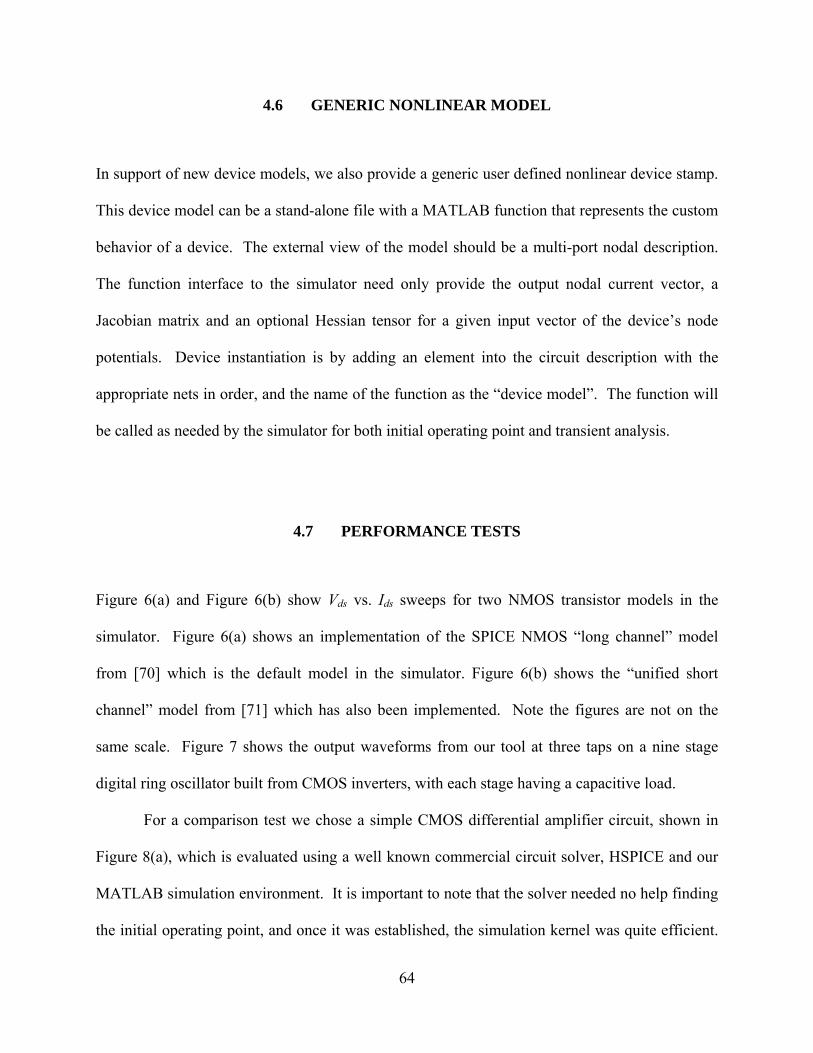
64
4.6 GENERIC NONLINEAR MODEL
In support of new device models, we also provide a generic user defined nonlinear device stamp.
This device model can be a stand-alone file with a MATLAB function that represents the custom
behavior of a device. The external view of the model should be a multi-port nodal description.
The function interface to the simulator need only provide the output nodal current vector, a
Jacobian matrix and an optional Hessian tensor for a given input vector of the device’s node
potentials. Device instantiation is by adding an element into the circuit description with the
appropriate nets in order, and the name of the function as the “device model”. The function will
be called as needed by the simulator for both initial operating point and transient analysis.
4.7 PERFORMANCE TESTS
Figure 6(a) and Figure 6(b) show Vds vs. Ids sweeps for two NMOS transistor models in the
simulator. Figure 6(a) shows an implementation of the SPICE NMOS “long channel” model
from [70] which is the default model in the simulator. Figure 6(b) shows the “unified short
channel” model from [71] which has also been implemented. Note the figures are not on the
same scale. Figure 7 shows the output waveforms from our tool at three taps on a nine stage
digital ring oscillator built from CMOS inverters, with each stage having a capacitive load.
For a comparison test we chose a simple CMOS differential amplifier circuit, shown in
Figure 8(a), which is evaluated using a well known commercial circuit solver, HSPICE and our
MATLAB simulation environment. It is important to note that the solver needed no help finding
the initial operating point, and once it was established, the simulation kernel was quite efficient.
65
On average, the solver took three iterations to converge at each timestep, compared to an average
of two iterations per timestep for HSPICE. As before both responses are very close to each other
with large differences associated with the initial transient, as presented in Figure 9(a) and Figure
9(b). The different nature for the initial operating point estimation for both solvers is the most
likely cause for these divergences.
Vds (V) Vds (V)
Figure 6. Ids sweeps using (a) Long Channel [70] and (b) Short Channel [71] models (different scales)
For a second test we chose an astable multivibrator circuit, shown in Figure 8(b), which
is also evaluated using HSPICE (MOS model level 1) and our MATLAB simulation
environment (MOS model level 1). The HSPICE simulations used level 1 parameterized MOS
models. The SPICE description was directly parsed into the MATLAB format, including the
model parameters and run in the simulator. As shown in Figure 10(a) and Figure 10(b), both
HSPICE and our simulator found initial conditions and simulated the circuit breaking into
oscillation. However, in this case different (but both valid) initial conditions were determined by
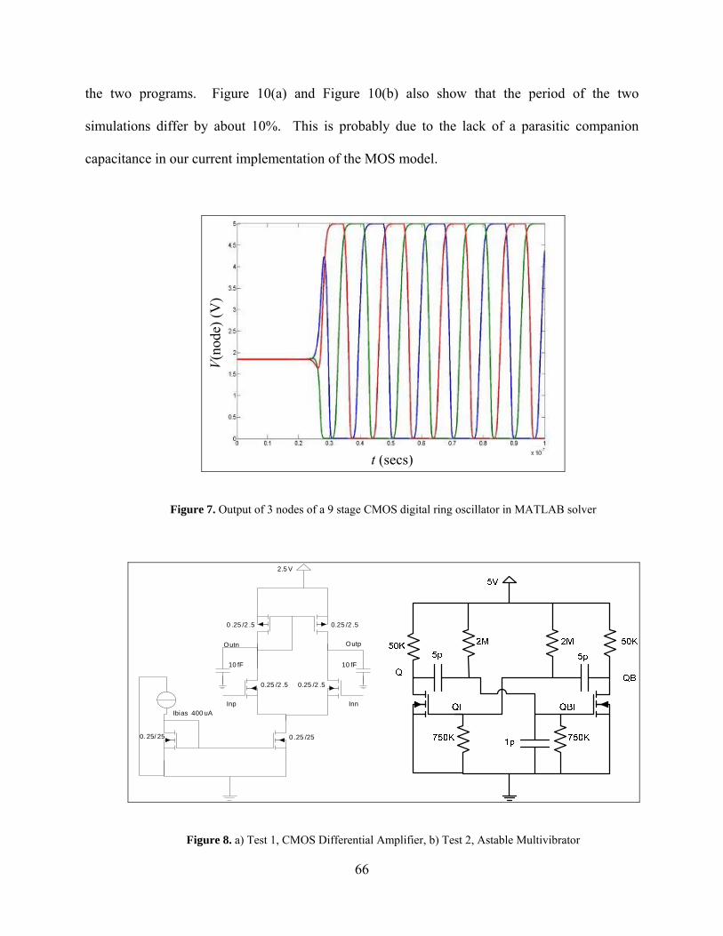
66
the two programs. Figure 10(a) and Figure 10(b) also show that the period of the two
simulations differ by about 10%. This is probably due to the lack of a parasitic companion
capacitance in our current implementation of the MOS model.
t (secs)
V
(nod
e) (
V)
Figure 7. Output of 3 nodes of a 9 stage CMOS digital ring oscillator in MATLAB solver
Inp Inn
OutpOutn
2.5 V
Ibias 400 uA
0 .25 /2 .5 0.25 /2 .5
0.25 /2 .50.25 /2 .5
0 .25 /250. 25/ 25
10 fF10 fF
Figure 8. a) Test 1, CMOS Differential Amplifier, b) Test 2, Astable Multivibrator
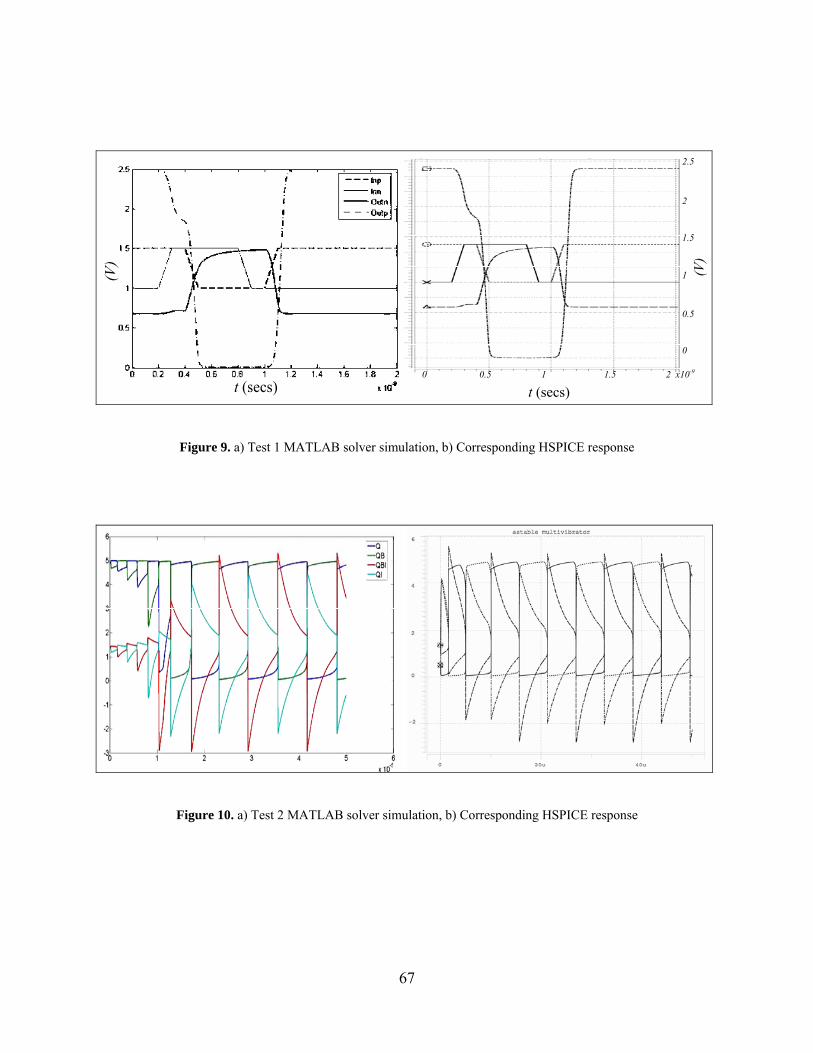
67
(V
)
t (secs)
1
2
0
1.5
0.5
2.5
0 1 2 x10-90.5 1.5
t (secs)
(V
)
Figure 9. a) Test 1 MATLAB solver simulation, b) Corresponding HSPICE response
Figure 10. a) Test 2 MATLAB solver simulation, b) Corresponding HSPICE response

68
4.8 SUMMARY
In this chapter we have presented the development and operation of our MATLAB based analog
solver. The resulting simulation platform shows results that are comparable in accuracy to well
known circuit solvers when we use the same models for the elements under simulation. It is
obvious that the slower execution time of the algorithm in the MATLAB environment is a
consequence of the overhead of the modeling platform. However, it does offer comparable
performance in terms of the number of iterations per evaluation as a cost measurement.
The presented MATLAB platform can be used for the investigation of both new models
and new simulation techniques compatible with existing SPICE models of devices and netlists of
circuits and systems. This will enable device designers to develop MATLAB models and
perform circuit simulation of devices based on new circuit fabrication techniques and new
material systems including nanoelectronics, molecular electronics, organic semiconductors,
carbon nanotube devices, etc. This environment also serves us as the tool for the implementation
and evaluation of the new methodologies proposed in this work for the reduction of very large
nonlinear systems.

69
5.0 TRAJECTORY PIECEWISE-LINEAR MODEL ORDER REDUCTION
METHOD
In this chapter we describe the trajectory based piecewise-linear technique for the model order
reduction of large nonlinear systems first introduced by White et al. in [3]. This methodology
has been recently developed as a practical approach for the generation of compact models for
these types of dynamic systems. Our interest resides in the use of this approach as a starting
point in following chapters for the development of a more optimal strategy to deal with such
problems. After initially describing the algorithm and the details surrounding the ensemble
reduced order model that it generates, we illustrate its advantages and limitations with the help of
a series of test cases.
5.1 TRAJECTORY PIECEWISE-LINEAR METHODOLOGY
Trajectory Piece-wise Linear Model Order Reduction (TPWL) was introduced by Rewienski and
White [3][42] as an extension to the simpler strategy of reducing a large nonlinear system from a
single point linear approximation (Section 2.4.1). The main limitation of a single point MOR
strategy for a nonlinear system is that the accuracy of the approximation is limited to how far the
evaluation of the model is from the selected point for characterization. To solve this limitation,
Rewienski includes the use of multiple points in the state-space of the nonlinear system to

70
generate an equal number of linear approximations. With this set of linear approximations we
have now extended the range of applicability of the final model.
It is not difficult to see that the simplest approach to overcome the limitation on accuracy
of modeling the nonlinear function by a linear approximation at a single point is to use a multi-
point strategy. However, the question to answer, if this path is chosen, is where in the domain of
the nonlinear system under study we need to sample the state-space to obtain a good
characterization.
The volume of a very large dimensional space requires a prohibitively large number of
samples if we chose to use a homogeneous discretization strategy. It is straightforward to realize
that for a given volume, V , in a space NS , the total number of samples required K , grows
exponentially with the number of dimensions (i.e., NkK ), where k is the number of samples
per spatial dimension. This situation is clearly shown in Figure 11-a) for the 3D case, where to
equally divide the volume of space under study we require a large number of regions. Each sub-
region of space is shown as a spherical bubble that represents the volume of space where the
linear model for that region is valid. This is a very costly proposition considering that for the
systems in which we are interested the dimension of the space considered can be very large
(e.g., 000,10N ).

71
Linear expansion regions Training Trajectory
Expansion points a) b)
Figure 11. Training trajectories in the TPWL reduces the required number of bubbles in the state-space
The approach used in TPWL is to consider only tracks through the state-space that the
function moves through when the system is excited with typical inputs. These tracks in the state-
space (as shown in Figure 11-b)), also known as training trajectories by the authors, are used in a
first step of the method for the definition of the linearization point locations that are used as the
center for the derived linear regions.
The authors are consequently avoiding the difficulty of dealing with the large volume of
the original state-space realization by using these specific training trajectories. Under this
strategy, the proposed solution is specially tailored for the volume of the state-space that is in the
neighborhood of the selected training trajectory. The justification for this approach, as suggested
by the authors, is that the model functionality is confined and accordingly conditioned by the
input set commonly employed in the system.

72
Now that the original nonlinear system has been transformed into a set of linear models,
we can reduce these linear approximations to a smaller state-space through the use of a suitable
projection base. Finally, in order to obtain a compact model for this system, the individual
models in the set need to be connected in a single representation. To merge these sets of reduced
partial models, the authors use an empirical function that weights the contribution of each
component. The weight assignment is dependent on the Euclidian distance (2ixx ) between
the current state and each state used to generate the linear models in the set. The effect of this
weight function is a swift transition between sub models when the assembled model is used.
5.2 ALGORITHM
The strengths in the TPWL methodology are derived from two well established fields: the mature
area of reduction techniques for linear systems and second, but no less important, the rich
leverage of linear analysis knowledge. It offers a simple and practical avenue for the solution to
the problem of compact generation of nonlinear systems. It is desirable, however, to develop a
firm mathematical basis for this field as solid and well understood as in the linear field. As
previously mentioned there are currently efforts to develop a theoretical foundation for nonlinear
system minimization and from it a solid and consistent reduction methodology.
However, at this time, we consider that this approximation through linear snapshots
offers us a good base upon which to improve and gain further understanding of the still unclear
theoretical background for this field. In following chapters we discuss the limitations present in
this technique and offer improvements to address these drawbacks. Through this process we not

73
only offer a more robust methodology but also reach a better understanding of concepts related
to the field of nonlinear model order reduction.
Consequently, we now describe the TPWL method in detail. The algorithm in its
different components is presented followed by a performance evaluation through selected test
cases.
Given a very large nonlinear system in a state-space representation as presented in (5-1),
defined in the region NX , our goal is to find a compact model defined in a state-space
qZ where Nq .
xCy
tBuxfxET
)()(
(5-1)
Where Nx
is the state-space vector, My
is the output vector, Stu )( is the input
vector, NxNE is a storage matrix and, NxSB and NxMC are connectivity matrices for
the input and output of the system respectively. And )(xf
is a nonlinear function defined as
NNf : .
Let us define a linear approximation of )(xf
by regions defined at a specific location in
the state-space kx :
,)()( ikk xxJxfxf kxx toclose for (5-2)
The expression in (5-2) corresponds to the first two terms of a Taylor series expansion of
)(xf around kx where kJ is the Jacobian of the function.
Consequently, expression (5-1) transforms to a series of sub models (i.e., linear sub-
models) that accurately describe the system in the vicinity of the respective expansion points:

74
xCy
tBuxxJxfxE
tBuxxJxfxE
tBuxxJxfxE
T
kkk
),()()(
),()()(
),()()(
222
111
,
,
,
2
22
21
Txx
Txx
Txx
k
(5-3)
Not having any reason to prefer one direction over another in the state-space, the
Euclidian distance 2/1
kk xxd is used to define the proximity between the current evaluation
state x and the expansion point kx .
The authors propose the use of a scalar function dependent on kd to weigh the
contribution of each of the sub-models into a final ensemble. The reader can visualize this as an
activation function that turns on and off the expressions in (5-3) according to the proximity of the
current evaluation to the expansion locations. This activation, however, is a smooth operation
that allows the easy transition from one region to the next. This is important since this model
requires evaluation using an analog solver. A non-continuous model is generally a cause for
troublesome or costly evaluation in the solver (i.e., a source of convergence problems)
This weight function evaluated over the set of expansion points, { kx }, corresponds to a
weight vector )(xw defined as:
,])(,..,)(,)([)( 21T
kxwxwxwxw ,1)(1
k
iixw (5-4)
Where in order to conserve the original system (5-1) after the ensemble, the total
contribution of the weight effect is unitary.
Using (5-4) to merge the contributions in (5-3) gives us the following expression:

75
xCy
tBuxJxwxJxfxwxE
T
k
iii
k
iiiii
),()())()(()(11 (5-5)
Let us define Q as the vector of independent sources generated as a consequence of the
linearization:
],))()(())()(())()(([ 222111 kkk xJxfxJxfxJxfQ (5-6)
This gives us a more compact form for (5-5):
xCy
tBuxwQxJxwxE
T
k
iii
),()(.)(1 (5-7)
This expression is the linear assembly of sub-models that can now undergo a reduction
process using a projection technique.
Considering that we have obtained a pair of biorthonormal projection bases U and V
(e.g., through Krylov based techniques or Truncation methodology, Section (2.3.2 -2.3.3)) we
can apply a suitable projection to (5-7):
zCy
tuBzwQzJzwzE
Tr
rr
k
iirir
),()(.)(1 (5-8)
Where the reduced state vector is related to the original as Vzx , and the matrices by
EVUE Tr , VJUJ i
Tir , QUQ T
r , BUB Tr , ,VCC TT
r
In this formulation it is evident that the result, as proposed, is a group of k linear reduced
models that have been developed from the expansion of selected state-space locations ix . )(xw
is the weight expression as a function of the state separation )( izz .

76
5.3 WEIGHT FUNCTION SELECTION
The characteristics imposed by the authors on the nature of this function give a wide range of
possibilities for its selection. The function should approximate the unit when the distance to the
pivot or expansion point for the region is close to zero. Its behavior in the opposite situation (far
from its point) should be close to zero. Furthermore, we want this behavior to be fast (i.e., super
linear in distance). The steps chosen to generate the weight function in the original TPWL
method are:
,_/)()(
,)(_
,))min(/)(exp()(
,
1
25
2
wsumxwxw
xwwsum
ddxw
xxd
ii
k
ii
iii
ii
Where an exponential function, dependent on the Euclidian distance between state and
pivot, is used for the weight and a final step of normalization is applied to satisfy the need that
there is no scaling of the original system.
5.4 FAST TRAINING APPROACH
Since the training phase of the TPWL algorithm involves the evaluation of the original large
system to produce the trajectory in the state-space, it can be a very computationally costly
procedure. To alleviate this cost it has been proposed to use a “fast training” approach for this
methodology [3]. The fast training approach is based on the premise that we do not need an
exact location in the state-space to generate a corresponding suitable expansion point in the
77
reduced state-space. That is, instead of evaluating the costly and large original system at every
point, we use the current reduced version. The practical effect is to project the linearized model
of the current region and use this compact model to move the system through the reduced state-
space. Granted, the approximated model only gives us an approximated trajectory to the real
one, but this approximation is in general a good selection to use for the next expansion point
location. The computational cost is now reduced to the linearization of the system for each
expansion point that has to be done from the original system and the smaller cost of an
evaluation in the smaller dimensional space z . We can summarize the fast algorithm as:
Step 1. Use projection base pair ],[ VU to generate a reduced model at ii zx
Step 2. Evaluate linear reduced model until ixVz (near the expansion point)
Step 3. Vzxi 1 , Use current state as new expansion point, return to Step 1 if not
finished
5.5 PERFORMANCE OF TPWL
In this section, a set of experiments have been chosen to show the accuracy and evaluation cost
of the TPWL when compared to the direct evaluation of the original system and other modeling
approaches.
We present two test systems selected to evaluate the performance of this nonlinear
modeling reduction technique. We then show the capability of the technique to provide compact
models whose behaviors closely match the original system behavior. We follow with a
discussion of the computational cost of the methodology when compared to the evaluation cost
of the large original counterpart.

78
Finally, we discuss the drawbacks of the technique which are responsible for some of the
marked differences observed between the output of the compact model and the real response.
5.5.1 Nonlinear test systems
We have selected two test systems to show the potential of this methodology in terms of
accuracy and computational cost when used to generate compact models: A nonlinear
transmission line (weakly nonlinear system), and a multistage CMOS inverter chain (highly
nonlinear system). An additional aim of these tests is to illustrate any limitations that the user has
to be aware of in order to reduce the chances of a poor characterization by these techniques. In
the following chapters we propose strategies to eliminate or minimize these drawbacks.
5.5.2 A nonlinear transmission line (RC nonlinear ladder)
We have selected as our first test example a nonlinear transmission line circuit, first proposed in
[3]. The n node circuit, shown in Figure 12, is a RC ladder with nonlinearities concentrated in
the elements, kId (a nonlinear diode). The current in these elements is defined as obeying the
following expression:
1)40exp()( vvIdk ,

79
Figure 12. Test system 1: A nonlinear transmission line [3]
Only a single input single output (SISO) representation is considered but the results are
easily extensible to the multiple input multiple output (MIMO) case. There is a single current
source i(t) as the input to the system in node 1, and there is also a single selected output, the
voltage, also at node 1. Without lost of generality and for simplification purposes, we use unit
values for the Gi (conductance) and the Ci, (capacitance).
5.5.2.1 Multi-stage CMOS Inverter Chain
Our second test system is a multi-stage CMOS inverter chain shown in Figure 13. The
nonlinearities in this system are more severe than in previous test bed, since the MOS devices in
the circuit are described by the nonlinear MOS FET model level 1 [70]. This implementation, a
long channel dominated behavior, is by no means restrictive, since any other model CMOS
description could be used instead. In order to force the system to operate in the nonlinear region,
we use large input signals that allow the elements to go beyond their linear regions.

80
Vs+
100fF InN OutN
5 V
Inv N
In2 Out2
5 V
Inv 2
In1 Out1
5 V
Inv 1
Figure 13. Test system 2: Multi-stage of CMOS Inverters. A simple CMOS inverter is presented in the right figure
and the cascade of units in the left figure
5.5.3 Tests of RC Ladder
For the first model system, the training signal used to generate this TPWL model is a unit pulse
in the input, i(t), in Figure 12. In Figure 14, the response of the system to this input is presented
along with the time location where the system characteristic is captured to generate a new region.
These locations are the pivots or expansion points for the algorithm. A snapshot of the system is
used to produce the corresponding reduced model through the projection base. To represent how
good these individual pivots recreate the output of the system, the projections of the next value
for the output using this single representation as linear models are also presented in the figure.
We can see that those individual models produce good approximations for points in their
proximity.
In Inv
5
In
Out In
M2 (2/20)
M1 (2/50)
In
5
Out

81
Figure 14. System Output for the training phase of the algorithm. Outputs for a full nonlinear system evaluation of
RC nonlinear ladder (N = 1500). The instants where an expansion point is generated are indicated by cross points as
well as the approximation of the output using the reduced state value. The total number of pivots or expansion
points used is 19 corresponding to an equal number of quasi-linear regions in the final TPWL model.
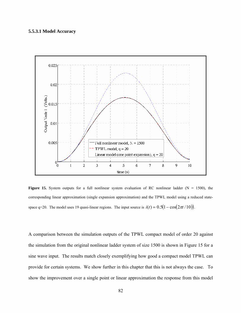
82
5.5.3.1 Model Accuracy
Figure 15. System outputs for a full nonlinear system evaluation of RC nonlinear ladder (N = 1500), the
corresponding linear approximation (single expansion approximation) and the TPWL model using a reduced state-
space q=20. The model uses 19 quasi-linear regions. The input source is 10/2cos15.0)( tti .
A comparison between the simulation outputs of the TPWL compact model of order 20 against
the simulation from the original nonlinear ladder system of size 1500 is shown in Figure 15 for a
sine wave input. The results match closely exemplifying how good a compact model TPWL can
provide for certain systems. We show further in this chapter that this is not always the case. To
show the improvement over a single point or linear approximation the response from this model

83
is also added in the figure. The single point model is obtained using a single linear
approximation for the nonlinear system and reducing this representation. This model output
degrades very quickly when the state of the system moves apart from that of the approximation
location at t=0.
5.5.4 Computational cost
In order to show the potential offered by this reduction methodology we use the nonlinear ladder
test system, with sizes 100, 400, 800 and 1500 nodes, and evaluate the cost of the simulation for
different model sizes. The original system is simulated using a full nonlinear analog simulation
(Full nonlinear), and using the reduced model from TPWL technique (TPWL MOR)2. The time
of completion of the different phases are presented in Table 2. These experiments are performed
with a setting that gives us 18 regions during model generation (training).
Table 2. Time comparison between TPWL technique and the full nonlinear evaluation for the nonlinear RC ladder
system, size 100, 400, 800, and 1500 nodes. 18 regions were used for all the cases.
2 All the simulations were accomplished using MATLAB, in a Linux workstation, Pentium 4/2.7 GHz/4 Gbyte RAM
System Size
Model (size)
Evaluation Time (s)
Generation Time (s)
Avg. Error (%)
RMS Error (%)
Max RMS Error
100 65.0433 (Full System)
N/A 0 0 0
25 1.69105 3.63774 0.68689 0.81872 1.75143 20 1.52156 3.91695 1.25088 1.69596 7.03896 10 1.52091 4.15465 2.74808 2.86992 4.26289 5 1.37674 3.60255 5.96276 6.30603 8.8383

84
Table 2 (continued).
In Table 2, we can see how TPWL offers a considerable gain in speed when the size of
the system is large. We are also including the cost associated with the generation of each model
during the training phase of TPWL. We need to clarify although that the generation time
indicated is the additional time over the time used for the full evaluation. We need to remember
that during the training phase we are doing a full evaluation of the system in addition to the extra
processing described in the training algorithm to identify new regions and generate reduced
model corresponding to that location.
In order to graphically observe the difference in speed we present this data in Figure 16.
For the case of a system of 100 nodes there is a gain in speed of ≈ 30X while when using the 800
400 1052.92 (Full System)
N/A 0 0 0
25 1.58455 123.086 0.67134 0.80034 1.67794 20 1.50646 135.478 1.23976 1.6898 7.04189 10 1.55183 135.544 2.73254 2.85311 4.18732 5 1.41807 126.595 5.94856 6.29253 8.79361 800 13302.2
(Full System) N/A 0 0 0
25 1.73006 1197.68 0.67134 0.80034 1.67794 20 1.5111 1176.47 1.23976 1.6898 7.04189 10 1.43797 1237.48 2.73254 2.85311 4.18732 5 1.36909 1212.77 5.94856 6.29253 8.79361 1500 77850.5
(Full System) N/A 0 0 0
25 1.58449 11107.6 0.67134 0.80034 1.67794 20 1.51851 11151.5 1.23976 1.6898 7.04189 10 1.40692 10965.6 2.73254 2.85311 4.18732 5 1.39982 11283.6 5.94856 6.29253 8.79361

85
nodes system we achieved a speed up of ≈ 7600X (when compared to the full system evaluation
time).
Nonlinear RC Ladder System, Evaluation Time
0
0.2
0.4
0.6
0.8
1
1.2
1.4
1.6
1.8
2
5 10 20 25
Size
Tim
e (
s) (N=100)
(N=400)
(N=800)
(N=1500)
Figure 16. Evaluation time for the TPWL modeling of the nonlinear RC ladder system. Four different model sizes
are considered q= 5, 10, 20 and 25. The number of regions is 18 for each model. Four system sizes are considered:
100, 400, 800 and 1500 nodes. Evaluation times for 100, 400 and 800 correspond to a full system evaluation are
found in Table 2.
In Figure 17 we show the error trends for the generated models (q = 5, 10, 20, 25) in the
previous set of experiments when compared to a full system evaluation. We show the % average
error and the % RMS error for each point. As expected for each system size (N =100, 400, 800
and 1500) we obtain an error that decreases when a larger model size is chosen. However, the
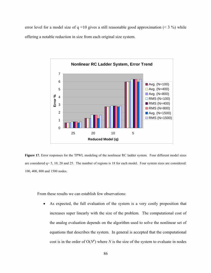
86
error level for a model size of q =10 gives a still reasonable good approximation (< 3 %) while
offering a notable reduction in size from each original size system.
Nonlinear RC Ladder System, Error Trend
0
1
2
3
4
5
6
7
25 20 10 5
Reduced Model (q)
Err
or
%
Avg. (N=100)
Avg. (N=400)
Avg. (N=800)
RMS (N=100)
RMS (N=400)
RMS (N=800)
Avg. (N=1500)
RMS (N=1500)
Figure 17. Error responses for the TPWL modeling of the nonlinear RC ladder system. Four different model sizes
are considered q= 5, 10, 20 and 25. The number of regions is 18 for each model. Four system sizes are considered:
100, 400, 800 and 1500 nodes.
From these results we can establish few observations:
As expected, the full evaluation of the system is a very costly proposition that
increases super linearly with the size of the problem. The computational cost of
the analog evaluation depends on the algorithm used to solve the nonlinear set of
equations that describes the system. In general is accepted that the computational
cost is in the order of O(Np) where N is the size of the system to evaluate in nodes

87
and p is the hyper linear exponent that range in 2<p< 3, which depends on the
used internal algorithm.
The cost of the generation of the TPWL is highly dependent on the size of the
problem and the number of regions requested. During the generation phase,
TPWL requires to compute Euclidian distances (O(N2)), and whenever a region is
found to extract the model (O(Nq) ), where N is the size of the full system and q
the size of the reduced model. The overhead associated with this phase (in
addition to the full evaluation cost) is dominated by the (O(N2)) and this is show
in Table 2, where this overhead grows with the size of the system. The cost of the
second term is not significant as can be seen by the little change between model
sizes when considering a single system size.
The cost associated with the evaluation of the reduced model is depending on two
factors: a) The cost related to the analog solver used for the evaluation which is
as previously mentioned on the order of O(qp) where q is now the size of the
system to consider, and p as before is in the range of 2<p< 3. b) The cost
associate with the weight evaluation for the combination of the sub regions. This
cost can be estimated to be on the order of O(q2s) where q is the size of the model
and s is the number of regions used in the model. Depending on the chosen
values of q and s one of these two terms could dominate the evaluation time for
the reduced model. In our particular set of test we can see from Table 2 a lightly
increase with the size of the model and this can be explained as to be shadowed
by the overhead of other (one time) operations in the algorithm.

88
The memory cost for the TPWL method is also )( 2sqO where s is the number of
quasi-liner models in the final TPWL ensemble and q is the size of the reduced
representation. This compares favorable with the cost of storage for the original
system, which is )( 2NO , where N is the original system size. If q is notably
smaller than the N, which is the original requirement, then the memory demand
for the compact representation is very small even for those situations where a
large number of regions are used for a good characterization of the system.
In summary, the simulation time of the reduced models when compared to the cost of the
full evaluation is several orders of magnitude smaller. As initially suggested, this is the main
advantage of using a smaller representation for the problem under study. Even when there is a
high cost, especially for the TPWL for the generation of this compact model, this is a one time
cost which is progressively less significant with the successive uses of the model and for longer
evaluation periods.
5.6 LIMITATIONS OF THE TECHNIQUE
Even when proven very effective for some systems, TPWL has shown a series of limitations that
make this method hard to apply for successfully obtaining compact realizations of large
nonlinear systems. It has already been mentioned that the TPWL technique is highly dependent
on the trajectory set used during the training stage [41][42][62] and that the error in the predicted
output for the reduced model is also dependent on the starting state value for the simulation. We
follow with a description of these limitations as well as others and a series of tests that show their
impact in typical operation:

89
Dependency on the chosen initial state: The initial state to use in the evaluation phase of
the method has to be guaranteed to be accurately contained in the target sub-space for the
reduced system. This requirement was already remarked by Rewienski in [3], when he
proposed to add this initial state as an additional vector-column to the projection base to use
in the reduction process. Since it forms part of the projection base, this guarantees its
presence in the reduced space. However this approach has an obvious disadvantage, the
required initial state has to be known beforehand to be included in the training process.
To illustrate this effect, we use TPWL to generate a reduced model of size 20 (q=20)
from the nonlinear ladder circuit of 400 nodes. The training conditions are the same as the
ones used in Section 5.5.2. In Figure 18 we show the output of the reduced model and the
output of the original system when the initial state matches the expansion state used to
generate the projection base used for the reduction. The two responses are closely matching
each other. In Figure 19, the same model is driven by a different input, where the initial state
is not perfectly captured in the reduced space. A clear error is added to the response and
easily identifiable in the figure, shown in more detail in Figure 20.
The cause of this effect is the initial error introduced in the evaluation process by the
projection of the initial state into the reduced space. This error introduced in the evaluation
process can cause the system to drift off the correct response. Since there is no mechanism
for error recovery in the TPWL methodology, the continued behavior of the model from this
point becomes unpredictable. Additionally, the projected state could not be a valid state in
the reduced state-space representation. In this later case any further advance from the initial
state is not possible.

90
Figure 18. If the state selected as the starting location in the evaluation phase in TPWL is completely contained in
the new state-space there is not initial error introduced to the system.
Figure 19. Effect of selecting as a starting point a state not fully contained in the reduced sub-space during the
evaluation phase of TPWL.
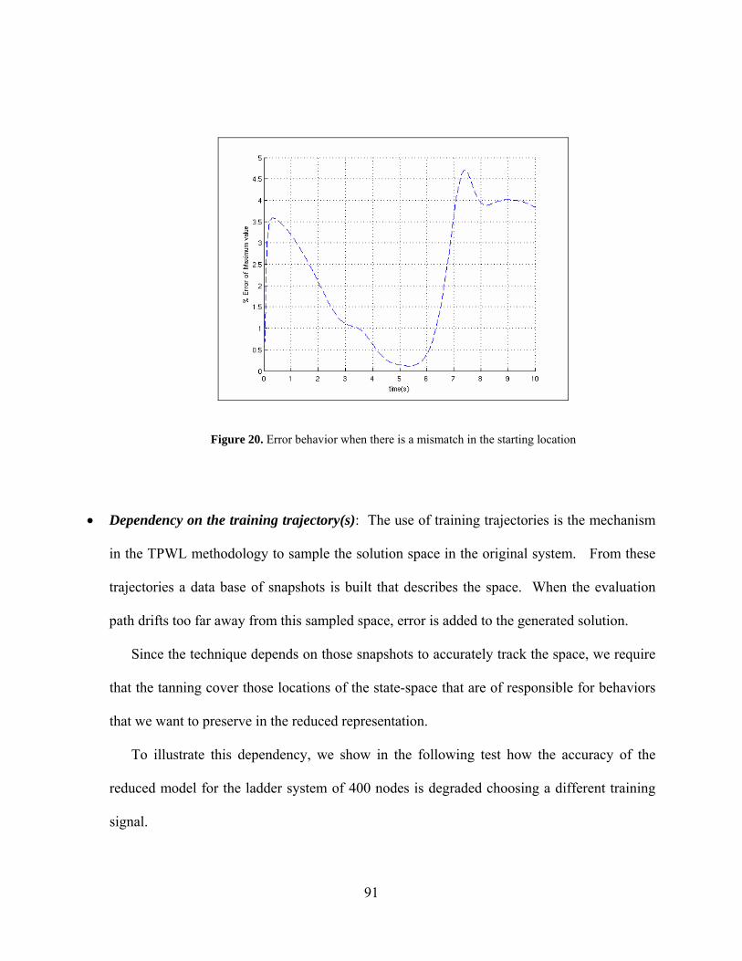
91
Figure 20. Error behavior when there is a mismatch in the starting location
Dependency on the training trajectory(s): The use of training trajectories is the mechanism
in the TPWL methodology to sample the solution space in the original system. From these
trajectories a data base of snapshots is built that describes the space. When the evaluation
path drifts too far away from this sampled space, error is added to the generated solution.
Since the technique depends on those snapshots to accurately track the space, we require
that the tanning cover those locations of the state-space that are of responsible for behaviors
that we want to preserve in the reduced representation.
To illustrate this dependency, we show in the following test how the accuracy of the
reduced model for the ladder system of 400 nodes is degraded choosing a different training
signal.

92
Figure 21. Training phase for the RC nonlinear ladder, N = 400. Training input is a unit step function.
Figure 22. Response of the reduced model (q=20) for the RC ladder (400 nodes) where the effect of a poor training
phase is shown. The response to a falling edge behavior of the input signal is badly captured.
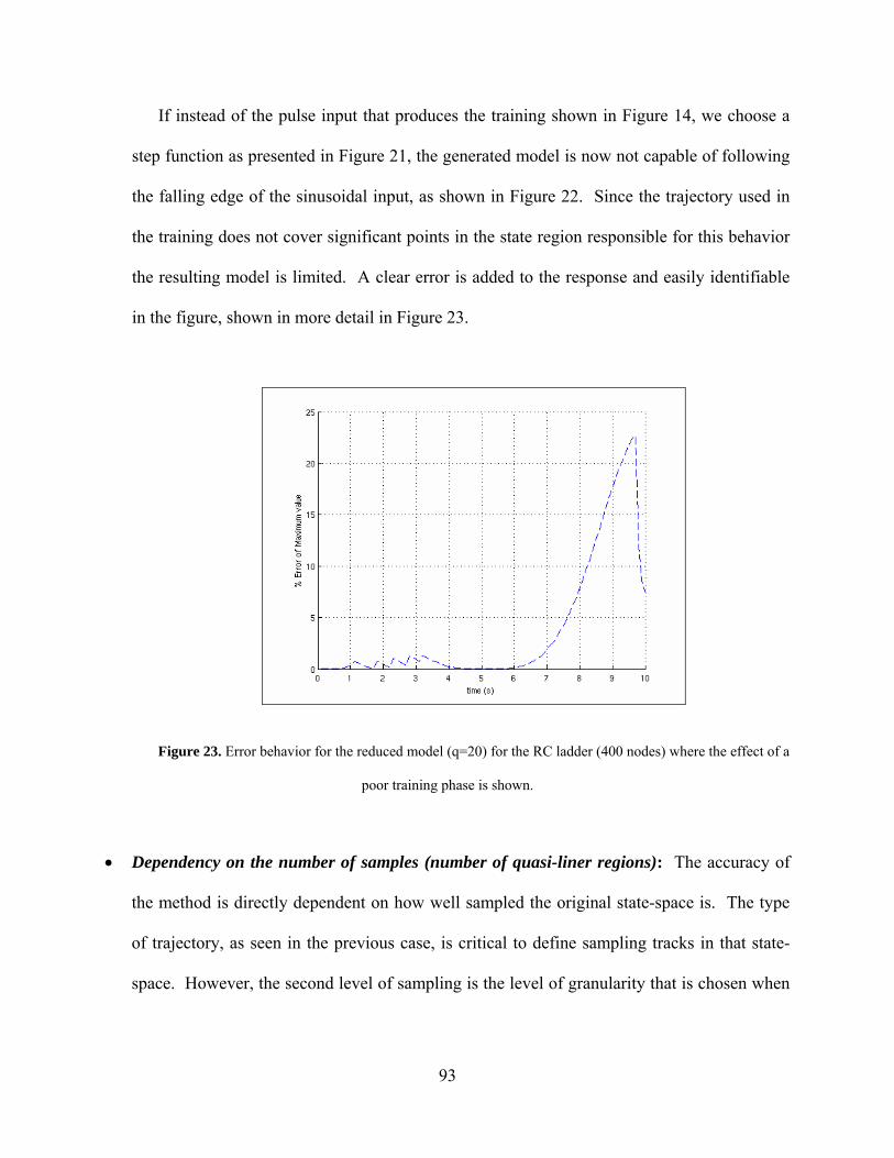
93
If instead of the pulse input that produces the training shown in Figure 14, we choose a
step function as presented in Figure 21, the generated model is now not capable of following
the falling edge of the sinusoidal input, as shown in Figure 22. Since the trajectory used in
the training does not cover significant points in the state region responsible for this behavior
the resulting model is limited. A clear error is added to the response and easily identifiable
in the figure, shown in more detail in Figure 23.
Figure 23. Error behavior for the reduced model (q=20) for the RC ladder (400 nodes) where the effect of a
poor training phase is shown.
Dependency on the number of samples (number of quasi-liner regions): The accuracy of
the method is directly dependent on how well sampled the original state-space is. The type
of trajectory, as seen in the previous case, is critical to define sampling tracks in that state-
space. However, the second level of sampling is the level of granularity that is chosen when

94
moving through a training trajectory. We can understand this as a second level in a 2 level
sampling strategy, which is what is used to cover the volume of interest.
To illustrate this dependency, we increase the radius for each defined region in the
previous test case. For this example we define only 4 regions instead of the 20 regions
previously used. Clear differences between the desired behavior and the response of the
model are shown in Figure 24 as the consequences of a coarser sampling.
Figure 24. Reduced model from RC nonlinear ladder, 400 nodes, generated using 4 regions
There are additional factors that affect the success of TPWL such as:
Dependency on the projection base used for the reduction process: We cover this
dependency in more detail in the following chapter.

95
Dependency on the characteristics of the weight function: The type of function used to
assemble the set of snapshots into the final model is what determines the behavior around the
“pivots”, how far is the reach for each region during the evaluation phase, and what the shape
of the merging of neighboring regions is.
5.7 SUMMARY
In this chapter we described the TPWL methodology for the model order reduction of nonlinear
systems. The technique is a marked improvement over the single-point linear expansion
technique proposed earlier [60] and shows good accuracy when dealing with a varied set of test
systems. Simplicity and the ability to quickly generate the quasi-linear regions using the fast
training algorithm are the main advantages of this work. However, we note that the technique
requires, in general, a good size number of trajectories to generate a good compact model for a
given region of study. Another limitation is the dependency on the proper selection of the
expansion points (pivots) for the quality of the resulting model. The TPWL methodology itself
does not give a procedure for the optimal selection of these points which introduces a degree of
uncertainty when trying to obtain a successful reduction. Additionally, for simplicity the model
uses the information from one of these pivots to generate the projection base to use for the whole
reduction process. This fails to consider alternative points that, because of the nature of the
state-space can be present at other points. In the following chapter we introduce modifications to
this technique that allows us to improve on these two drawbacks.

96
6.0 NONLINEAR PIECEWISE MOR USING MULTI-PROJECTION BASES
In Section 2.3.1 it was shown that a simple approach to achieve MOR of a very large nonlinear
system is to reduce its linear approximation. This approximation can be obtained by considering
only the linear terms of a Taylor series expansion at a chosen location of its state-space.
However, the accuracy of the resulting compact model is limited to those points in the proximity
of the selected expansion point. In the previous chapter we have shown one way to overcome
this limitation is through the use of multiple expansion points on selected locations in the state-
space of the system that are visited when the system is excited with a series of “typical” input
signals. This method, TPWL [3], increase the accuracy of the generated model through the
compound effect
In this chapter, we initially discuss the sources of error in the TPWL model order
reduction methodology with special emphasis on the error introduced by the use of a projection
base for the reduction process derived from a single expansion point. We show that the error
introduced by this simplification can be much more significant than the one corresponding to the
linear approximation itself.

97
To improve upon this limitation, we propose a methodology for incorporating in a final
optimized projection base the information contained in each of the linearized models from an
equal number of expansion points. Through a series of experiments, we then show the advantage
of this approach versus the traditional and simple single-point-single-base version of the
algorithm.
6.1 ERROR CONTRIBUTIONS IN SINGLE-PROJECTION BASE PWL MOR
In the piecewise linear MOR technique, which uses a projection base generated from a single
state-space location, there are three sources of error between the output of the reduced model and
the output of the original system under study:
Error by linearization: Because of the linear approximation at the expansion point (i.e.
quasi-linear model generation) the response of the resulting model tends to deviate from
the original when moving farther from the vicinity of this location. This error is the
motivation behind the modification of the algorithm to include multiple expansion points
and to assemble the final model from the resulting quasi-linear set.
Error by projection into the reduced state-space: As mentioned in Section 2.2.1 the
reduction of dimensionality on the original system is based in the assumption that the
contribution of a large number of the states can be mostly discarded without severely
affecting the system output. However, because of this truncation of non-relevant states
there is a small difference between the output of the reduced model and the original
98
system. The closeness between both outputs depends on how good the selected
projection base is in isolating the relatively significant contributions from the original
state-space representation.
Error by using a single point to generate projection base: There is an additional and very
significant source of error in a multi-point reduction strategy methodology such as
TPWL, the use of a projection base derived from a single linearization point. In the next
section we describe in detail this situation.
6.1.1 Limitation of a projection base V generated from a single expansion point in its use
in TPWL
We show in this section that the assumption that the projection base derived from a single quasi-
linear region (which is associated with a single expansion point 0x
) holds for the entire state-
space under study (i.e., the entire set of quasi-linear regions) is not a good option for the TPWL
methodology.
Let us remember that for the linear case of model order reduction, the premise is that we
can find a projection base that allows us to transform the given system into a compact
representation with a much lower dimensional state-space size. The reduction process can be
understood as the projection of the system from the large state-space where originally defined to
a smaller subspace while preserving its most significant behavior. If this projection base can be
found then the output of the resulting reduced model closely follows the output of the original
system.

99
For the nonlinear case of model order reduction and following the TWPL technique [3],
we approximate the nonlinear system by a set of quasi-linear regions to which we apply linear
MOR reduction. However, contrary to the linear case, the optimal projection base derived for
one region (i.e., which represents the optimal subspace to capture the system behavior in that
region) is in general non optimal for the rest of the regions in the set.
Figure 25. Error caused by the difference in subspace between two adjacent regions (3D interpretation)
A useful way to explain the limitation of a projection base, generated from a single
expansion point for nonlinear MOR, is to consider that the discarded state-space is a null space
from the point of view of the output of the system (i.e., the extra dimensions in this null subspace
nU
δ (Δ Subspace)
qiS
qjS
)(f

100
do not contribute to the response of interest). However, this assumption is only valid in the
neighborhood of the expansion point. In points farther from it, this discarded subspace could
hold significant contributions that worsen the accuracy of the generated model.
If we use the projection base derived from the information of a single region for the
reduction of neighboring quasi-linear regions, we are potentially introducing an error by
insufficiently capturing the behavior of the system in those other regions. In Figure 25, we show
a graphical representation of this case in a 3D perspective. Let us consider that qjS is the
optimal subspace that contains the nonlinear function nxf )( (described by a single
trajectory in the figure). Let us also consider that we chose to use the sub-optimal subspace
qiS instead of jS for the projection of the system. The consequence of this selection is an
error by omission that is described in the figure by the orthogonal subspace d containing
the difference (i.e., the size d of this subspace represents the number of states that the reduction
fails to capture).
Figure 26, a) A trajectory of the nonlinear system with two defined neighboring quasi-linear regions, i and j, b)
Graphical representation of the subspace for the two regions, Si and Sj, and mutual relationship.
NSNS ji ijcji SSS
ijcS
iS
jS N
nN
xoj , Vj
x0i , Vi
i region
j region
)(f
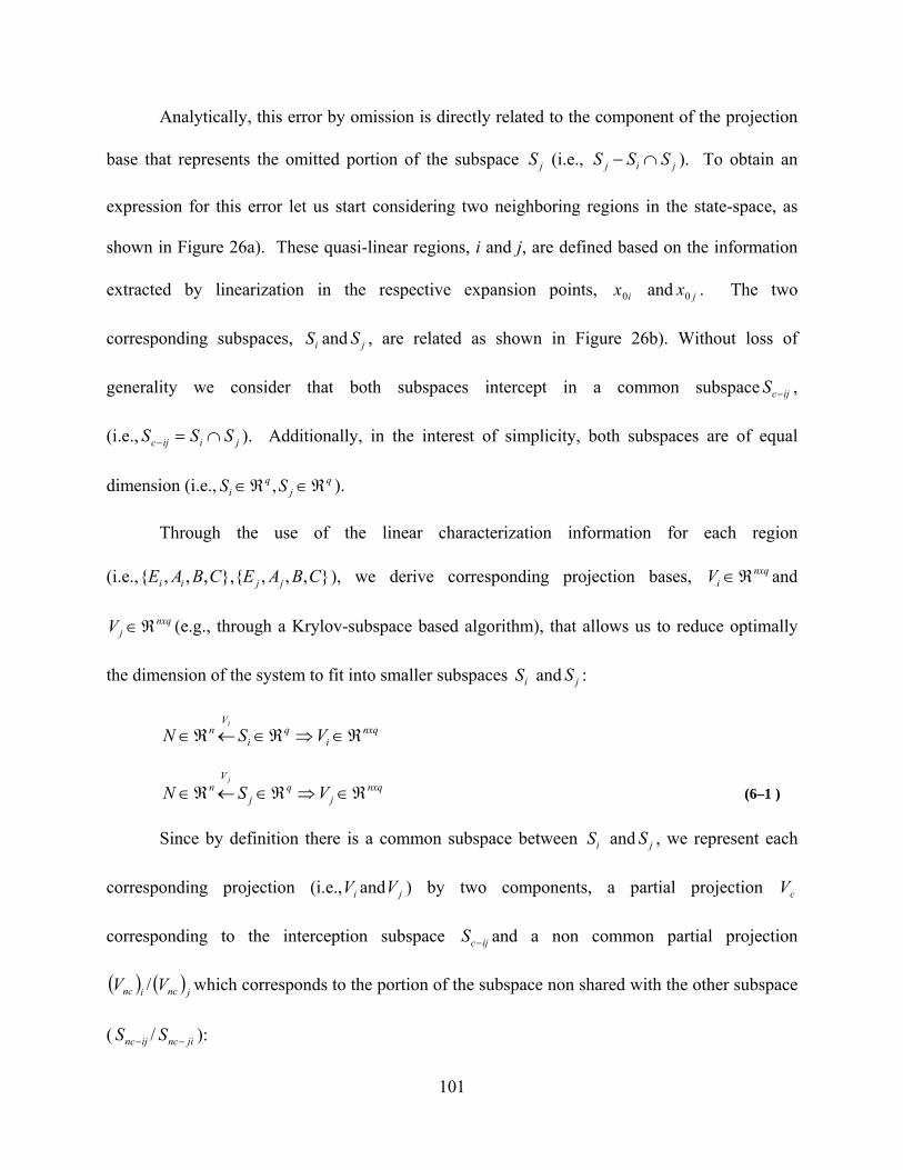
101
Analytically, this error by omission is directly related to the component of the projection
base that represents the omitted portion of the subspace jS (i.e., jij SSS ). To obtain an
expression for this error let us start considering two neighboring regions in the state-space, as
shown in Figure 26a). These quasi-linear regions, i and j, are defined based on the information
extracted by linearization in the respective expansion points, ix0 and jx0 . The two
corresponding subspaces, iS and jS , are related as shown in Figure 26b). Without loss of
generality we consider that both subspaces intercept in a common subspace ijcS ,
(i.e., jiijc SSS ). Additionally, in the interest of simplicity, both subspaces are of equal
dimension (i.e., qj
qi SS , ).
Through the use of the linear characterization information for each region
(i.e., },,,{},,,,{ CBAECBAE jjii ), we derive corresponding projection bases, nxqiV and
nxqjV (e.g., through a Krylov-subspace based algorithm), that allows us to reduce optimally
the dimension of the system to fit into smaller subspaces iS and jS :
nxqi
qi
Vn VSN
i
nxqj
qj
Vn VSN
j
(6–1 )
Since by definition there is a common subspace between iS and jS , we represent each
corresponding projection (i.e., iV and jV ) by two components, a partial projection cV
corresponding to the interception subspace ijcS and a non common partial projection
incV / jncV which corresponds to the portion of the subspace non shared with the other subspace
( ijncS / jincS ):
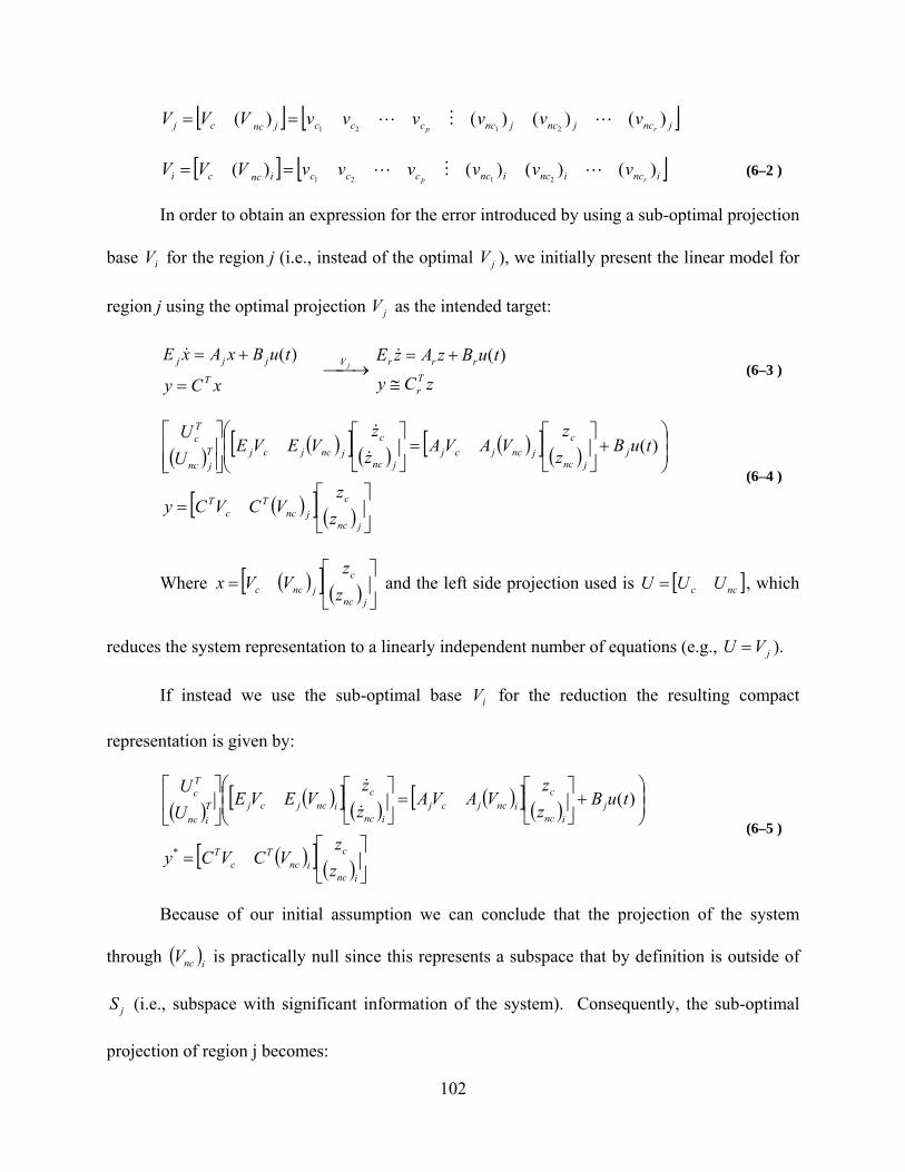
102
jncjncjnccccjnccj rpvvvvvvVVV )()()()(
2121
incincinccccincci rpvvvvvvVVV )()()()(
2121 (6–2 )
In order to obtain an expression for the error introduced by using a sub-optimal projection
base iV for the region j (i.e., instead of the optimal jV ), we initially present the linear model for
region j using the optimal projection jV as the intended target:
xCy
tuBxAxET
jjj
)( jV
zCy
tuBzAzETr
rrr
)( (6–3 )
jnc
c
jncT
cT
jjnc
c
jncjcjjnc
c
jncjcjT
jnc
Tc
z
zVCVCy
tuBz
zVAVA
z
zVEVE
U
U)(
(6–4 )
Where
jnc
c
jncc z
zVVx and the left side projection used is ncc UUU , which
reduces the system representation to a linearly independent number of equations (e.g., jVU ).
If instead we use the sub-optimal base iV for the reduction the resulting compact
representation is given by:
inc
c
incT
cT
jinc
c
incjcjinc
c
incjcjT
inc
Tc
z
zVCVCy
tuBz
zVAVA
z
zVEVE
U
U
*
)(
(6–5 )
Because of our initial assumption we can conclude that the projection of the system
through incV is practically null since this represents a subspace that by definition is outside of
jS (i.e., subspace with significant information of the system). Consequently, the sub-optimal
projection of region j becomes:
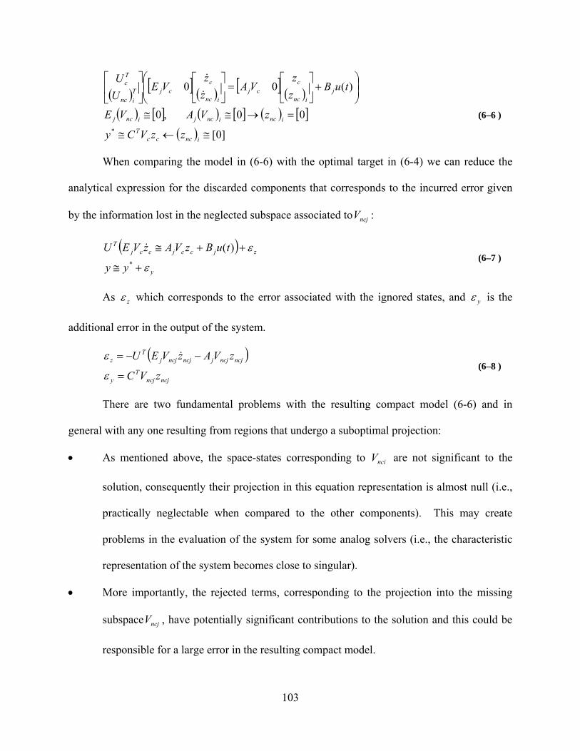
103
]0[
00 ,0
)(00
*
incccT
incincjincj
jinc
ccj
inc
ccjT
inc
Tc
zzVCy
zVAVE
tuBz
zVA
z
zVE
U
U
(6–6 )
When comparing the model in (6-6) with the optimal target in (6-4) we can reduce the
analytical expression for the discarded components that corresponds to the incurred error given
by the information lost in the neglected subspace associated to ncjV :
y
zjccjccjT
yy
tuBzVAzVEU
*
)( (6–7 )
As z which corresponds to the error associated with the ignored states, and y is the
additional error in the output of the system.
ncjncj
Ty
ncjncjjncjncjjT
z
zVC
zVAzVEU
(6–8 )
There are two fundamental problems with the resulting compact model (6-6) and in
general with any one resulting from regions that undergo a suboptimal projection:
As mentioned above, the space-states corresponding to nciV are not significant to the
solution, consequently their projection in this equation representation is almost null (i.e.,
practically neglectable when compared to the other components). This may create
problems in the evaluation of the system for some analog solvers (i.e., the characteristic
representation of the system becomes close to singular).
More importantly, the rejected terms, corresponding to the projection into the missing
subspace ncjV , have potentially significant contributions to the solution and this could be
responsible for a large error in the resulting compact model.
104
It is important to mention that this problem is only a mayor issue for highly nonlinear
behavioral systems. In the case of a weakly nonlinear system (i.e., a representation where the
resulting quasi-linear regions are spatially contained in an unique subspace) then it is possible to
use the projection base generated from any expansion points in the volume under study (i.e.,
essentially the same projection base) for the reduction process of the whole set of regions
without any appreciable lost of accuracy in the resulting compact model (i.e., the set of quasi-
linear regions are optimally confined in a single subspace inside of the volume of interest).
If we modify this methodology to generate a single projection base from the information
of the whole set of quasi-linear regions instead of just one particular region in the volume of
study, we believe that we can achieve a more accurate compact realization. Additionally, this
modification could potentially provide the optimal size for the reduced model that captures any
significant behavior from the original nonlinear system.
6.2 MULTI-PROJECTION BASE ALTERNATIVES FOR PWL MOR
In previous chapters the reduction process has been carried out using a single projection base
over the set of quasi-linear regions. This projection base is derived using the information from
one of the quasi-linear representations of the system. However, as mentioned previously this
consideration is a cause of error in the final compact representation if there are significant
differences between the derived projection bases from each individual quasi-linear region in the
set.
A better alternative is to use projection bases obtained for each individual region for the
reduction treatment of each region’s model. This strategy best captures the behavior of the

105
system in each region. However, there are two major problems when trying to combine the
resulting partial models into a single final combined model:
There is not a guarantee of continuity for the model when crossing regions. Since each
projection base establishes a specific state-space definition for that region, each region
state-space is in general not the same. Even for regions belonging to the same subspace,
the associated projection bases can differ and consequently the state definition. This is
because there are an infinite number of projection bases to describe the same subspace.
The concept of Euclidian distance would be meaningless when operating in different
subspaces, and consequently this would render the use of a weighting function for the
final assemble based in this parameter ineffective.
Consequently, it is desirable to use a single projection base for the whole set of regions
(eliminating continuity problems) that incorporates the system information gathered from the set
of quasi-linear regions. In the following section we provide a technique to merge these set of
projection bases into a single common base that can be used for the whole state-space volume of
the problem considered.
6.2.1 Extended projection base Algorithm
This method generates a projection base that defines a subspace qS that contains each
region state-space in the final assembled model. The column-vectors in this projection base S
represent each and every significant state in the resulting piecewise assembled model.
When evaluating a new region to be included in the final assembled model, the subspace
defined by its projection base is checked against the current subspace (defined by the current

106
projection base resV ). Any part of this subspace that it is not contained in the current subspace
represents a non common subspace that needs to be accounted for. The current projection base is
then updated with the addition of a suitable set of column vectors that expand this state-space
subset.
Given two regions iR and jR of the state-space nN where the nonlinear system
under analysis can be described by the following corresponding linear approximations:
)(tuBxAxE iii , )(tuBxAxE jjj (6–9 )
Let us establish the existence of respective projection bases nxqV and nxrU that
allows us to reduce these quasi-linear models in more compact representations that are contained
in corresponding smaller subspaces qS and rW (i.e., nrq ), where rq .
Two cases are possible when trying to establish a single projection base suitable for both
regions:
a. W is a subspace of S (i.e., W is contained in S , SW ).
b. W is not a subspace of S (i.e., W is not contained or fully contained in S , SW ).
We show in the following development the procedure to generate a common projection
base for case b) which is clearly the general case.
Let us examine now the general case represented in Figure 26b). In the more general
situation the optimal subspaces (i.e., those that contain the entire behavior of the system in the
region) corresponding to two neighboring regions could share a common subspace. The final
projection base that characterizes the optimal subspace for both regions is consequently the one
that corresponds to the combined subspace of both regions. The only information we have from
these subspaces is the one contained in their respective projection bases nxqiV and nxs
jV .

107
At this point it is necessary to remember that there exist an infinite number of orthogonal
projection bases related to the same single subspace. Any orthonormal linear transformation of a
projection base generates a valid projection base for the subspace under study. The first step in
the consolidation of projection bases is to find the communality between two given projection
bases and doing so define the non-common subspaces in the association.
To accomplish this, it is only necessary to use an orthogonalization algorithm to find the
non contained orthogonal column vectors between both projection bases. Let us describe a
simple algorithm to achieve this based on the Gram-Schmidt orthogonalization technique
[72][A-2].
Given two projection bases iV and jV :
qiiii vvvV
21 nxq
iV
sjjjj vvvV
21 nxs
jV (6–10 )
Where iV represents the larger subspace (i.e., q> s)
In this algorithm, each of the orthogonal column-vectors kjv representing a state in the
subspace given by jV is decomposed into the state-space defined by iV . The residual of this
operation represents the subspace not contained in iS . This reminder is normalized to define the
column vectors for the not shared subspace.

108
Algorithm:
The output of this algorithm is the desired projection base expV , which corresponds to the
optimal subspace for the combined region models:
rq ncncnciiinci vvvvvvVVV
2121exp )(exp
rqnxV (6–11 )
Where nxrncV represents the additional subspace that was not contained in iS .
This procedure is repeated over the whole set of projection bases from quasi-linear
regions to generate an optimal projection base from the whole set of projection bases. Clearly
the algorithm is additive with a result that is a projection base that corresponds to the union of
the whole set of subspaces.
The result of this aggregative process is a final projection base that is suitable for the
entire evaluated region. However, this aggregated base could potentially grow in size to the
maximum size allowed N (size of the system). In order to bring back the base to a practical size
1. Initialize: iVV exp , qn
2. Gram-Schmidt reduction over jV from each vector in expV
for sk :1
jknvtv
1exp
for nz :1
zzjnn
vvvtvtvk expexp1exp1exp ).(
// Normalize residue if over tolerance (TOL)
if 1expn
tv TOL
1exp1exp1exp /
nnn
tvtvv , 1 nn
end
end
end
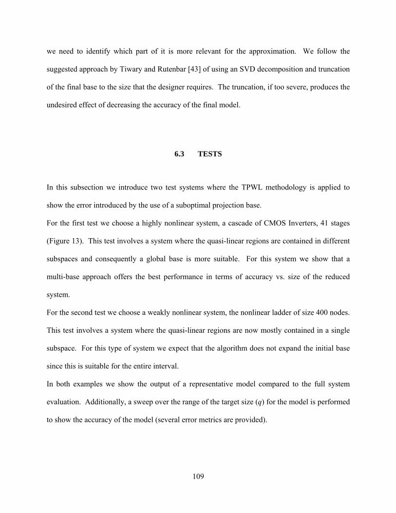
109
we need to identify which part of it is more relevant for the approximation. We follow the
suggested approach by Tiwary and Rutenbar [43] of using an SVD decomposition and truncation
of the final base to the size that the designer requires. The truncation, if too severe, produces the
undesired effect of decreasing the accuracy of the final model.
6.3 TESTS
In this subsection we introduce two test systems where the TPWL methodology is applied to
show the error introduced by the use of a suboptimal projection base.
For the first test we choose a highly nonlinear system, a cascade of CMOS Inverters, 41 stages
(Figure 13). This test involves a system where the quasi-linear regions are contained in different
subspaces and consequently a global base is more suitable. For this system we show that a
multi-base approach offers the best performance in terms of accuracy vs. size of the reduced
system.
For the second test we choose a weakly nonlinear system, the nonlinear ladder of size 400 nodes.
This test involves a system where the quasi-linear regions are now mostly contained in a single
subspace. For this type of system we expect that the algorithm does not expand the initial base
since this is suitable for the entire interval.
In both examples we show the output of a representative model compared to the full system
evaluation. Additionally, a sweep over the range of the target size (q) for the model is performed
to show the accuracy of the model (several error metrics are provided).

110
6.3.1.1 Performance of Multi-Projection base on highly non-linear system
In order to show the improvement on the accuracy of the generated model when using a
multi-projection base strategy, we compare the model generated using a single base and the
model generated using the multi-base approach over the CMOS inverter chain test case. This
test case is composed of 41 stages of CMOS inverters in a cascade configuration (Figure 13).
The total size of the system is 44 nodes and for illustrative purpose in Figure 27 we present a
generated model of size q=8 using a single projection base strategy at the first expansion point
versus a similar response, shown in Figure 28, of a model of size q=6 generated using a multi-
base approach that combines the bases on the 60 expansion points used in this test. The training
and evaluation phases are conducted after the system is in steady state, further from the setup
time or delay introduced by the signal propagation path in the chain.
When comparing the response of both models against the full system response, we can
see that the multi-base model gives us a better matching of the output of the system specifically
in the high level response. The single base-model is not able to be a good match in all cases
during this evaluation. We should emphasize that the conditions for both situations are identical
with the only difference being the projection base generated as the compounded effect of single
projections at each expansion location.

111
Figure 27. CMOS Inverter Chain, 41 Stages, 44 nodes. Model of size q=8, generated using a Single base modeling
approach for TPWL.
Figure 28. CMOS Inverter Chain, 41 Stages, 44 nodes. Model of size q=6, generated using Multi-base modeling
approach for TPWL

112
We should also clarify that for the multi-base case there are two parameters to specify
that contribute to the desired size of the final model. The first parameter is the intended size for
each projection base generated when the training algorithm evaluates a possible new sub-region.
Since the training algorithm is now building a final base through aggregation by the
orthogonalization algorithm of any non-contained column vector in each new projection base
found, the final size of the combined base could be large. Consequently, the second parameter
needed is the desired size for the projection base from this aggregated base. As previously
mentioned single value decomposition is applied to the combined base and a truncation base can
be derived with the first k most significant single values.
For this experiment it was found that requesting to match the first 5 moments on the
individual projection base through the block projection base algorithm was enough to provide a
good matching at each expansion point. Finally, the aggregated base size was large enough that
we can request different sizes from it. For the result shown in Figure 28 a size 6 was chosen.
The next analysis is to show not a single case for this experiment but to sweep the
possible range of sizes on the generated model and compare their accuracy using both
approaches. Figure 29 and Figure 30 show the performance of the resulting model for both
methodologies when we do a sweep over the target size (q) for the model. In these tests the
average error %, the root mean square % error (RMS) and the maximum RMS value are
provided. Each percentage is computed in relation to the maximum output value that is also
shown in the graphs.
It is interesting to note that in order to achieve a low RMS error value (< 5%) using a
single projection base we are forced to consider a target model of size q>=26. On the other hand

113
the multi-base approach allows one to obtain good approximation in the output for low values of
q. Almost each size of q >= 5 provide a RMS error value lower than 1%.
CMOS Inverter Chain 44 Nodes, (5<q<43)
0
5
10
15
20
25
0 10 20 30 40 50
q
Avg. Error %RMS Error %Max RMS Error %Max. Output (Volts)
Figure 29. TPWL Single projection base: Error vs. size (q) (The error values at q=3 were over 25% so this point is
dropped for better visualization).
Additionally, there is no guarantee that the single expansion point approach can always
generate a projection base that can achieve an acceptable level of error in the target model, since
the system information at that location could be incapable of generating a projection base that is
applicable to the whole range of the state-space that is used. For highly nonlinear systems the
need for a multi-projection base approach is not only an improvement but a requirement to fully
capture the overall system behavior.
We should also mention the behavior of the error average shown in Figure 30. From the
figure the best model is achieved with a size q= 6-7, and further from this point the error tends to

114
be somehow larger (≈ 0.5 % RMS compared to the lower 0.21 % RMS in q=6-7). The reason for
this according to what we have gathered through this pool of experiments is that the additional
state-space spanned by the increase on base size does not contribute to any additional
information useful for this simulation. Numerically this translates into an over-dimensioned
system to solve that has a tendency to accumulate numerical errors. Consequently, the system
output becomes noisier and the computation time is needlessly increased.
CMOS Inverter Chain 44 Nodes, (5<q<35)
0
1
2
3
4
5
6
7
8
0 10 20 30 40
q
Avg. Error %RMS Error %Max RMS Error %Max. Output (Volts)
Figure 30. TPWL Multi-projection base: Error vs. size (q) (The error values at q<=5 were over 9% so these points
are dropped for better visualization).
6.3.1.2 Performance of Multi-Projection base on weakly non-linear system
In this section we want to show the behavior of the multi-projection base approach when
dealing with a weakly non-linear system. For this experiment we have chosen the non-linear
ladder system with a size of N = 400 nodes. In Figure 31 we show the good matching of a
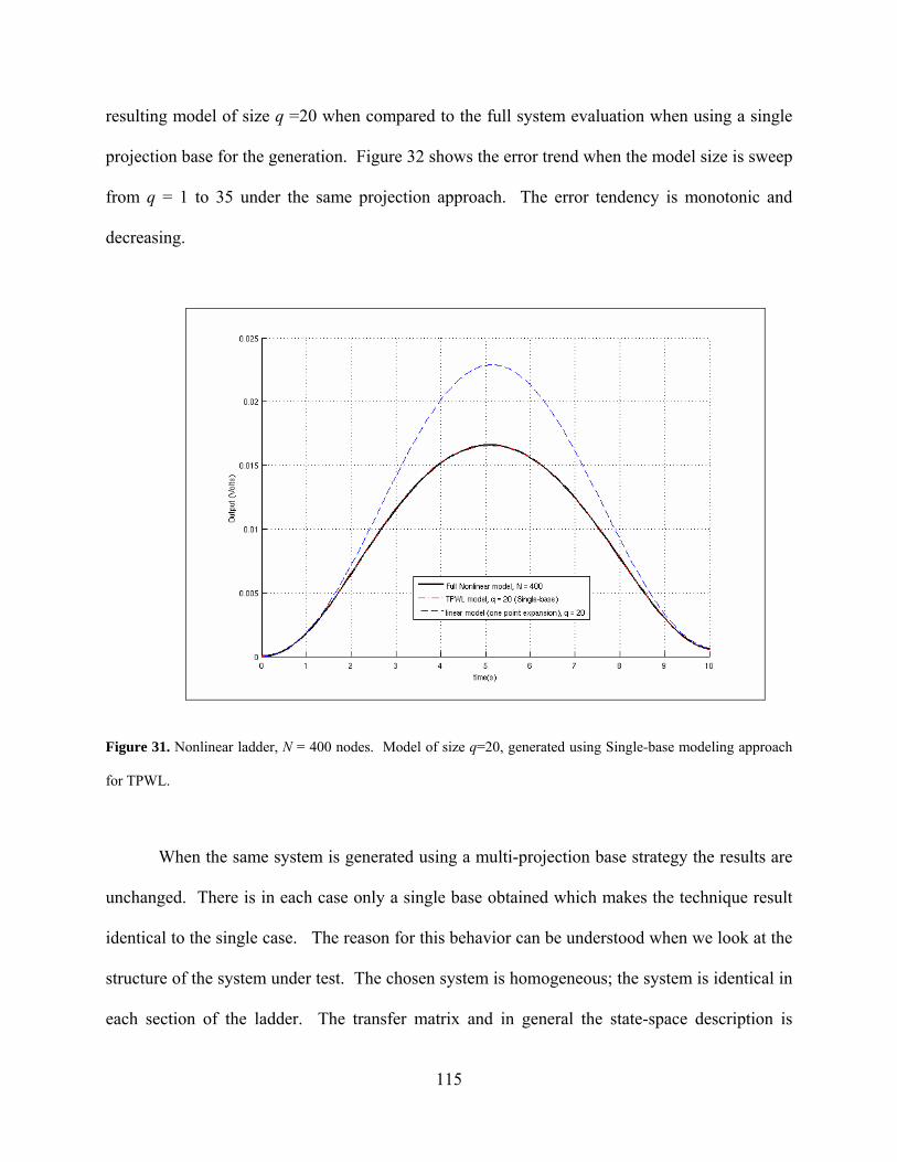
115
resulting model of size q =20 when compared to the full system evaluation when using a single
projection base for the generation. Figure 32 shows the error trend when the model size is sweep
from q = 1 to 35 under the same projection approach. The error tendency is monotonic and
decreasing.
Figure 31. Nonlinear ladder, N = 400 nodes. Model of size q=20, generated using Single-base modeling approach
for TPWL.
When the same system is generated using a multi-projection base strategy the results are
unchanged. There is in each case only a single base obtained which makes the technique result
identical to the single case. The reason for this behavior can be understood when we look at the
structure of the system under test. The chosen system is homogeneous; the system is identical in
each section of the ladder. The transfer matrix and in general the state-space description is

116
homogeneous as well. The block Arnoldi is reduced to operate as a single Arnoldi projection
algorithm since there is only a single source in the system and its result is the same in each
expansion point. There is not advantage in using small size bases in each expansion location to
aggregate to a final larger base since all of these individual bases are the same.
Consequently, there is not added value to the model for weakly nonlinear systems when
using a multi-projection base strategy, as theoretically is expected since the problem is mostly
contained in a single subspace, and there is an extra computational cost added to the training
phase nevertheless.
NonLinear Ladder 400 Nodes, (1<q<35)
0
5
10
15
20
25
30
35
40
0 10 20 30 40
q
Avg. Error %RMS Error %Max RMS Error %Max. Output (Volts)
Figure 32. TPWL Single-projection base: Error vs. size (q)

117
6.3.1.3 Computational cost of the Multi-Projection strategy
The cost for this addition to the methodology is entirely in the training phase. The
evaluation phase it is not affected in any way by this modification since we are still providing a
single base for the final model. In the training phase the cost associated with the multi-base
approach is two-fold. On one hand we now need to extract a single projection base per
expansion point and to add the projection base to the global projection base using the modified
Gram-Schmidt orthogonalization algorithm. On the other hand we need to apply SVD to the
final aggregated base in order to truncate to the desired final size.
The cost associated with the base extraction is dependent on the projection base
extraction algorithm implemented. An Arnoldi based algorithms, like the one used in this work
for the extraction of the projection base, has a reported cost in the order of O(Np), where N is the
size of the system and 2<p<3. The main cost associated with this type of algorithms is that they
require evaluating the inverse of the transformation matrix A (size N). The cost of the inverse
computation is in the order of O(Np) and it depends on the algorithm in place for its
implementation. Additionally, the SVD operation is a costly mathematical operation also on the
order of O(Np), where N in this case corresponds to the largest index of the passing matrix. In
our proposal, this step is a one time operation. In conclusion, the computational cost of these
modifications could be substantial for the training phase of the algorithm when we are faced with
very large size system.
However, we need to emphasize that the main reward of this or any other technique is in
a) a better accuracy performance in the final model or b) a smaller size of the reduced model that
translates into a faster evaluation.
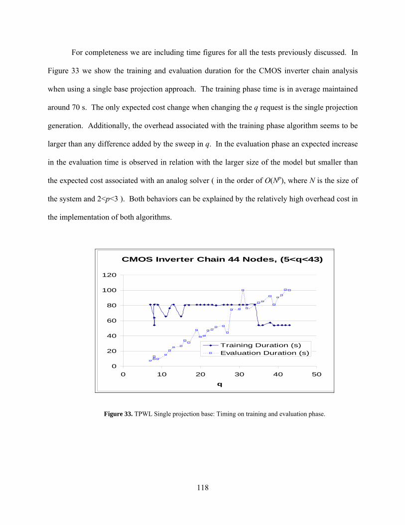
118
For completeness we are including time figures for all the tests previously discussed. In
Figure 33 we show the training and evaluation duration for the CMOS inverter chain analysis
when using a single base projection approach. The training phase time is in average maintained
around 70 s. The only expected cost change when changing the q request is the single projection
generation. Additionally, the overhead associated with the training phase algorithm seems to be
larger than any difference added by the sweep in q. In the evaluation phase an expected increase
in the evaluation time is observed in relation with the larger size of the model but smaller than
the expected cost associated with an analog solver ( in the order of O(Np), where N is the size of
the system and 2<p<3 ). Both behaviors can be explained by the relatively high overhead cost in
the implementation of both algorithms.
CMOS Inverter Chain 44 Nodes, (5<q<43)
0
20
40
60
80
100
120
0 10 20 30 40 50
q
Training Duration (s)Evaluation Duration (s)
Figure 33. TPWL Single projection base: Timing on training and evaluation phase.
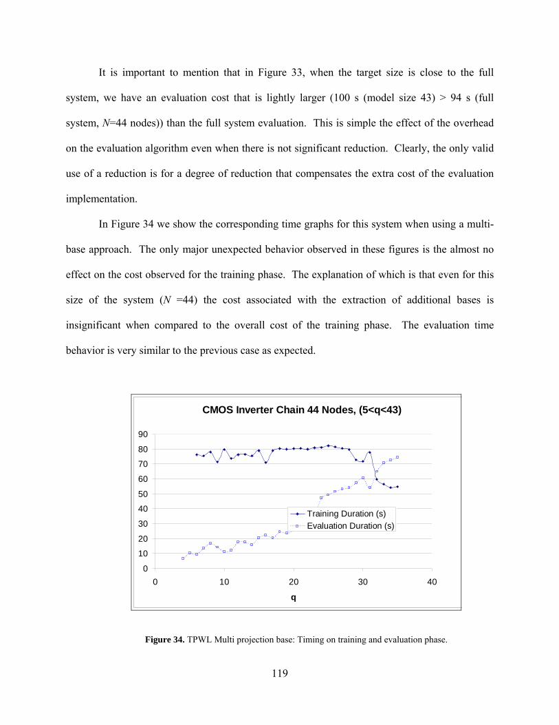
119
It is important to mention that in Figure 33, when the target size is close to the full
system, we have an evaluation cost that is lightly larger (100 s (model size 43) > 94 s (full
system, N=44 nodes)) than the full system evaluation. This is simple the effect of the overhead
on the evaluation algorithm even when there is not significant reduction. Clearly, the only valid
use of a reduction is for a degree of reduction that compensates the extra cost of the evaluation
implementation.
In Figure 34 we show the corresponding time graphs for this system when using a multi-
base approach. The only major unexpected behavior observed in these figures is the almost no
effect on the cost observed for the training phase. The explanation of which is that even for this
size of the system (N =44) the cost associated with the extraction of additional bases is
insignificant when compared to the overall cost of the training phase. The evaluation time
behavior is very similar to the previous case as expected.
CMOS Inverter Chain 44 Nodes, (5<q<43)
0
10
20
30
40
50
60
70
80
90
0 10 20 30 40
q
Training Duration (s)
Evaluation Duration (s)
Figure 34. TPWL Multi projection base: Timing on training and evaluation phase.

120
And finally, in Figure 35 a)-b) we present the timing graphs for the case of a nonlinear
ladder with single projection base approach. The training cost is relatively constant as
previously discussed and in the evaluation time we see the overall gain in speed of evaluation
when reducing the size of the model, main advantage of TPWL in general (as for comparison the
average cost of the full evaluation for this case is ≈ 109 s ).
NonLinear Ladder 400 Nodes, (1<q<35)
0
20
40
60
80
100
120
140
160
0 10 20 30 40
q
Training Duration (s)Evaluation Duration (s)
NonLinear Ladder 400 Nodes, (1<q<35)
0
1
2
3
4
5
6
7
8
9
10
0 10 20 30 40
q
Evaluation Duration (s)
Figure 35. TPWL Single projection base: a) Timing on training and evaluation phase b) Timing in evaluation phase.
6.4 SUMMARY
In this chapter we have analyzed the limitations present in the TPWL method [3] when a
projection base obtained from a single state value in the nonlinear system under study is used for
the entire reduction process [Section 6.1]. In Section 6.1.1 we developed a mathematical
expression for the error in the compact model approximation when using a suboptimal projection

121
base for the treatment of a quasi-linear region. A single projection base is desirable since
translates in a common subspace for the whole set of quasi-linear regions assemble to conform
the reduce model. Consequently, there are no continuity problems when the model transits
through its different sub-models.
In order to overcome the previous limitation, in Section 6.2 we developed a methodology
that allows us to incorporate the information derived from several expansion points from equal
numbers of quasi-linear regions into a single projection base. This projection base allows us to
efficiently capture the behavior of the nonlinear system through the whole set of quasi-linear
region models. As a result of this technique we can derive a model with a more accurate
response and additionally optimize its state size.
We then compare this modification to the single base projection case in two different
system cases: a high nonlinear system, cascade of CMOS inverters, and a weakly nonlinear
system, Nonlinear RC Ladder. In order to validate the impact of the multi-base approach a
sweep of the range of possible reduced size for the generated model was performed on both
cases. The error trends shows that the multi-base option allows one to capture very well the
performance of highly nonlinear systems with relatively small single base projection extractions
(lower computational cost) that combine into a final optimal projection base. However, for the
weakly nonlinear test, as expected, there was not improvement on the generated model. The
resulting effect is an increase in the computation cost associated with the training phase of the
method.
Finally, we discuss the computational cost associated with this addition to the TPWL
methodology. The cost is in the order of O(Np), where N is the size of the system and 2<p<3 for
the training phase and it could become expensive if the N of the system is very large. However,

122
we have to emphasize that the cost of the training phase is the natural penalty for these types of
methodologies.
Table 3. TPWL Multi projection base: CMOS Inverter Chain 44 nodes. Speed up vs. Error for different model sizes.
Model Size (q) Speed Up Avg Error % RMS Error % 44 (Full System) 1 0 0
35 1.263927 0.407389 0.726033 30 1.547027 0.407315 0.726012 25 1.905908 0.36312 0.692519 20 3.575626 0.546417 0.95128 15 4.537904 0.501379 0.93571 10 8.428351 0.679941 0.968383
9 6.605979 0.679941 0.968383 7 6.905023 0.213504 0.384526 6 9.750823 0.213504 0.384526
In Table 3, for the CMOS Inverter chain (44 nodes) system, we show the speed up in
relation with the full evaluation of the system when using different values for the size of the
reduced system. Even for this system of moderate size a close to 10x speed up can be achieved
with a relatively small penalty in accuracy in the generated model (0.2 %, q = 6). As previously
mentioned if the reduction degree is small the achieved speed up is not significant and it turns to
a slow performance (<1) when the overhead associated with the combination of the sub models
is larger than any saving in computation time because of reduction in size. It is normally
expected that with increasing size of the reduced model the accuracy improves, however in this
table we see that the performance is improving when reducing the size of the model. This is the
result of the multi-projection approach for this test as seen in Figure 30.

123
The best accuracy is obtained for a size q = 6-7. As mentioned before in section 6.3.1.1,
any additional increase in the size of the final model does not add information for this evaluation,
but potentially increases the likelihood for numerical errors.
The advantage of this or similar approaches is to consider that there is a single time cost
for the training phase and potentially a much larger repetitively use for the generated model.
This overall target is intended to replace the large full system during evaluation and this is where
the computational gain is achieved.

124
7.0 OPTIMIZATION OF EXPANSION POINT LOCATION IN NONLINEAR
PIECEWISE MOR
In this chapter we initially present the need for a technique to optimize the selection of the
locations of the state-space of the large space nonlinear system used as expansion points for the
generation of quasi-linear models in the TPWL. We describe how in the traditional methodology
for trajectory based PWL model order reduction, the selection is based in an arbitrary selection
of the permissible radius for the spherical bubbles of state-space used to define the quasi-linear
regions in the model.
We then follow with a description of the sources of error in this technique and how local
errors in the evaluation of the reduced model could potentially contribute to an accelerated
drifting phenomenon from the real behavior of the system.
As a mechanism to control the accuracy in the TPWL we introduce the notion of using
the Hessian of the nonlinear function to derive a figure of merit that allows both a way to judge
the degree of linearity of the region and to estimate a radius of validity for the volume defining
this.
The rest of the chapter consists in the derivation of a limit for the quasi-linear region
(multidimensional bubble) that is based on defining an error bound for the Taylor series
expansion of the nonlinear function used to model the region. We choose the Lagrange
remainder as an error bound for the truncated Taylor series expansion which corresponds to a
125
direct dependency to the Hessian of the nonlinear function. After the formulation of the required
radius limit we follow with a series of tests of this mechanism against the traditional fixed radius
in the TPWL technique. Finally we conclude the chapter with a summary of the performance of
this new technique that introduce a higher level of optimization to the technique of piecewise
linear modeling of large nonlinear systems.
7.1 NEED OF A STRATEGY FOR OPTIMIZING THE LOCATION OF EXPANSION
POINTS DURING THE TRAINING STAGE OF TPWL
We have shown in previous chapters that the accuracy in the expected behavior for the reduced
nonlinear model largely depends in the number of expansion points used to generate it. This is
because the expansion points correspond to locations in both the reduced state-space of the
compact model and the large state-space of the original system where the behavior of the system
in relation to the desired output matches. In simple terms, the more matches in the contour of the
hyperspace surface on both spaces we have, the smaller error in the behavior obtained from the
reduced model. Another interpretation that is used further in this chapter is that the behavior of
the reduced nonlinear model and consequently its quality depends on the chosen granularity or
density for this sampling in the training process (i.e., number of samples per unit of volume).
During the training process we are sampling the state-space of the original nonlinear
system (i.e., large dimensionality) looking for representative points in its response that capture
the intricacies of its behavior so we can carry those into the reduced state-space. However, in
TPWL [3] the criteria for selecting where to approximate the solution through linearization
which correspond to an expansion state point is based on a fixed and rather arbitrary limit on the
126
Euclidian distance to the closest expansion point. The net effect of this strategy is a uniform
discretization of the state-space. Where this strategy is the simplest to implement it does not
offer any opportunity to sample efficiently/optimally the state-space.
If the sampling tolerance is too loose the resulting reduced model incurs in large errors
during the evaluation stage, this effect does not only produce corresponding errors in the desired
output but, as we will detail further in the chapter, it is a potentially accumulative phenomena
that create a drift in the resulting trajectory that further increase the overall error in the model.
As a result of this equally spaced sampling strategy the only mechanism to increase the
accuracy on the resulting reduced model is to increase the granularity on the training process. As
mentioned in section 6, this corresponds to an increase in the number of trajectories used in the
training process which translates into a larger number of quasi-linear models in the final model
and additionally a proportionally longer computational time during the training process itself.
Furthermore, the increase in the granularity does not guarantee that we are able to capture all the
significant behaviors in the volume of space cover by the training stage.
Tiwary and Rutenbar [43][44][45] have proposed several enhancements to the original
TPWL that optimizes the use of large number of samples gathered during the training process.
Their scalable interpolation technique introduces the pruning of similar trajectories from the
original pool and the creation of a hierarchical database that allows for the use of few nearest
neighbors during the weight computation.
Following a different path to the problem of optimal distribution of samples during the
training path, we propose to use the second order term in the Taylor expansion (i.e., Hessian) to
define a figure of merit for the intended expansion point. This metric gives us information
corresponding to the behavior of the Jacobian of the nonlinear multidimensional function at this

127
location. The Jacobian corresponds for all practical purpose to the transformation matrix A in
the quasi-linear model for the region, consequently a measurement of how steady it is give us an
estimation of a) the degree of nonlinearity b) and the possible range of validity for the model.
7.2 ERROR ANALYSIS IN TRAJECTORY BASED PWL MODEL ORDER
REDUCTION
7.2.1 Error Sources in Multi-Projection PWL Model Order Reduction
The sources of error in the PWL model order reduction technique can be separated into two
major components: a) the approximation introduced by the linearization itself b) the error
introduced by the projection into the reduced space.
The error in the linearization process is an inherent weakness of any piecewise linear
technique. The direct approach to minimize this error is the inclusion additional samples points
where the deviation is larger than the allowed tolerance.
The error consequence of the projection process is inherent in the reduction process. It is
the penalty of throwing away the set of states whose contribution is considered minimal to the
desired output.

128
However, if the projection base is derived from the linear approximation obtained in a
single expansion point there is no guarantee that is the best subspace to optimally contain the
behavior of the system. The information of the system must be gathered from several of the
whole set of expansion points in order for the generation process to capture enough information
from the system behavior and to generate a projection base that capture the desired behavior of
the system.
7.2.2 Local Error and Global Error in TPWL
A situation observed in the previous chapter is that the TPWL technique for the generation of a
reduced model using a composition of linear models is highly sensitive to local errors during the
evaluation stage. The fact that the reduced model would have an error when compared to the
original system is expected. However, what is noteworthy is that the model does not provide a
way to recover from local errors. Consequently, the effect is accumulative and in the worst case
unpredictable.
Local errors in the TPWL technique are especially critical because the behavior of the
model is critically dependent of these 'anchor points' (i.e., expansion points) which correspond to
snapshots from the original large space system. These points correspond to locations of
maximum synergy with the original system, locations where we expect the error of being
minimal. However, because TPWL does not offer a mechanism for error correction or to give us
an error bound of the system at the current state, local errors corresponds to drift of the system
from the systems true trajectory that could bring larger global errors, not only because of the
accumulative effect but also by affecting the contributions of the individual quasi-linear models

129
themselves since the weighting of these are correlated to the distance to individual expansion
points. We follow with our proposed strategies to minimize this problem in TPWL.
7.3 PROPOSED STRATEGY TO MINIMIZE ERROR IN TPWL
There are locations in the state-space where variations (i.e., errors) in the estimation of the state-
value can have a profound effect in the subsequent behavior of the system. Consequently, it is
not just the magnitude of the error at those locations that is relevant but also perhaps more
important how tolerant the system is (i.e., sensitive) to that variation. In the volume of the space
where this sensitivity is high the model requires a major density for the number of samples (i.e.,
a larger number of expansion points and consequently of quasi-linear regions), otherwise the
requirement is more loose.
Consequently, if we follow the original PWL technique the only approach to minimize
this 'drift' is to increase the density of regions (i.e., increase of the number of samples from the
original system). Because there is not a mechanism to control the region radius or bubble size in
the model, this translate in a uniform distribution of samples that depends on the training
volume. This results in very expensive realizations even if the region of high sensitivity is a
small portion on the entire volume of interest. The more sensitive region will define the degree
of granularity for the whole training space. This adds to the reasons to increase the sample size
of the operating space which is done with a prohibitively large number of training trajectories.
We propose in this work a better approach, to adjust the permissible radio for the quasi-
linear region for each expansion point by an estimation of the degree of linearity in the evaluated
expansion point. For this we propose the use of the Hessian of the nonlinear representation in

130
addition to the Jacobian in already use in the TPWL methodology. The Jacobian characterizes
the linearity of the region and the Hessian gives us a measure of the linearity at that location.
TPWL technique does not provide a strategy to select the location for expansion points.
These locations are selected [3] according to a permissible radius for the region that is only based
on factor over the maximum Euclidian distance of the state vectors over the whole training
trajectory. This clearly is a uniform distribution of regions through the state-space regardless of
the behavior of the studied system. The only advantage of this approach clearly is simplicity but
a more optimal treatment for the definition of where to locate those expansion points and the
sides of the corresponding linear regions would account for a lower error bound for the resulting
assembled model. Nevertheless it is important to remark that the only strategy to correct
excessive divergence when using this simple linear region definition is to increase the number of
sampled points in the training process (and so doing being more accurate in the picking of
possible expansion points) and defining an small linearity radius to increase the behavior capture.
Both of these strategies are just brute force approaches that pour more information in the
resulting by force of numbers. We follow with the development of an expression for the
estimation of this linearity limit for the regions in the expansion set in TPWL.
7.3.1 Hessian as a figure of merit for the linearity of a quasi-linear region
We propose to use the information carried by an additional term (2nd term) of the Taylor
expansion of the nonlinear system at the current location 0x
to derive a limit for the range (i.e.,
radius of the spherical multidimensional volume) of the quasi-linear region.
As an error bound for a Taylor expansion we choose to use the Lagrange reminder factor.
Deriving an expression for this term allows us to have an upper limit to the error added by the 1st

131
order approximation used in the definition of the derived model. Because the Lagrange
remainder depends on the Euclidian distance from the point of expansion to the location for the
maximum order term in the approximation, we can estimate the permissible radius from the
actual location that gives us a region with an error under a predefined tolerance.
Given a very large nonlinear system in a state-space representation as presented in (7-1):
xCY
tBuxfxET
)()(
(7-1)
)(...)())((2/1)()()( 1000000 xRxxxxxHxxxJxfxf n
(7-2)
Which undergoes a linear expansion at a location 0x
(as shown in (7-2)), find an upper
limit r defined as the Euclidian distance between the state-space value x
of the system and the
expansion point 0x
, 20xxr
where the error of the approximation is below a given
tolerance level.
7.3.1.1 Mathematical convention used for the Hessian of a multidimensional vector function
The Hessian of a function ),...,,( 21 nxxxf , designed as )(H , is defined as a matrix that contains
the second order derivatives of f with respect to its states ),...,,( 21 nxxx given in the following
arrangement:
nnnnn
n
n
xx
f
xx
f
xx
f
xx
f
xx
f
xx
f
x
f
xx
fxx
f
xx
f
xx
f
x
f
xfH
2
1
2
1
2
1
2
2
2
32
2
22
2
12
21
2
31
2
21
2
21
2
)((
(7-3)
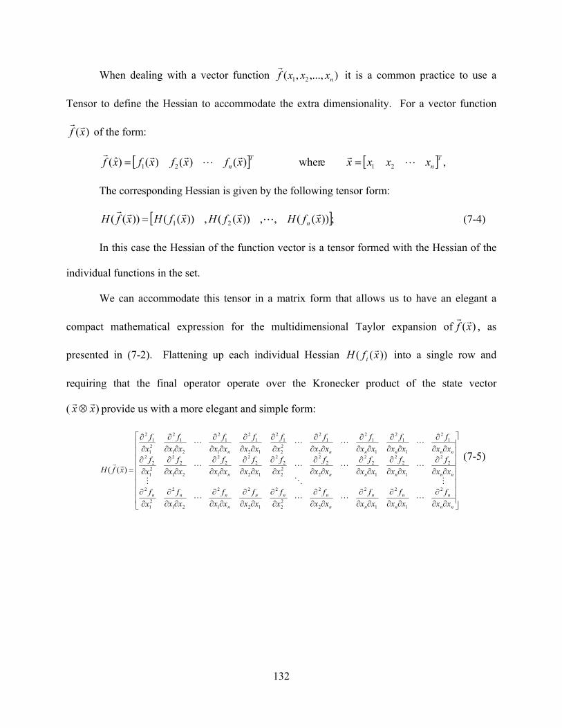
132
When dealing with a vector function ),...,,( 21 nxxxf
it is a common practice to use a
Tensor to define the Hessian to accommodate the extra dimensionality. For a vector function
)(xf
of the form:
, e wher )()()()ˆ( 2121T
nT
n xxxxxfxfxfxf
The corresponding Hessian is given by the following tensor form:
;))((,,))((,))(())(( 21 xfHxfHxfHxfH n
(7-4)
In this case the Hessian of the function vector is a tensor formed with the Hessian of the
individual functions in the set.
We can accommodate this tensor in a matrix form that allows us to have an elegant a
compact mathematical expression for the multidimensional Taylor expansion of )(xf
, as
presented in (7-2). Flattening up each individual Hessian ))(( xfH i
into a single row and
requiring that the final operator operate over the Kronecker product of the state vector
( )xx
provide us with a more elegant and simple form:
nn
n
n
n
n
n
n
nnn
n
nnn
nnnnnn
nnnnnn
xx
f
xx
f
xx
f
xx
f
x
f
xx
f
xx
f
xx
f
x
f
xx
f
xx
f
xx
f
xx
f
x
f
xx
f
xx
f
xx
f
x
fxx
f
xx
f
xx
f
xx
f
x
f
xx
f
xx
f
xx
f
x
f
xfH
2
1
2
1
2
2
2
22
2
12
2
1
2
21
2
21
2
22
1
22
1
22
2
22
22
22
12
22
1
22
21
22
21
22
12
1
12
1
12
2
12
22
12
12
12
1
12
21
12
21
12
)((
(7-5)
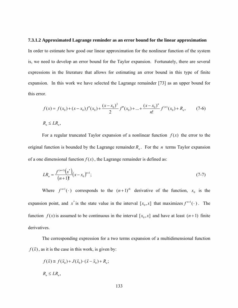
133
7.3.1.2 Approximated Lagrange reminder as an error bound for the linear approximation
In order to estimate how good our linear approximation for the nonlinear function of the system
is, we need to develop an error bound for the Taylor expansion. Fortunately, there are several
expressions in the literature that allows for estimating an error bound in this type of finite
expansion. In this work we have selected the Lagrange remainder [73] as an upper bound for
this error.
,)(!
)(...)(
2
)()()()()( 0
)(00
20
000 nn
n
Rxfn
xxxf
xxxfxxxfxf
(7-6)
,nn LRR
For a regular truncated Taylor expansion of a nonlinear function )(xf the error to the
original function is bounded by the Lagrange remainder nR . For the n terms Taylor expansion
of a one dimensional function )(xf , the Lagrange remainder is defined as:
;
!11
0
*)1(
nn
n xxn
xfLR (7-7)
Where ) (1 nf corresponds to the thn )1( derivative of the function, 0x is the
expansion point, and *x is the state value in the interval ],[ 0 xx that maximizes ) (1 nf . The
function )(xf is assumed to be continuous in the interval ],[ 0 xx and have at least )1( n finite
derivatives.
The corresponding expression for a two terms expansion of a multidimensional function
)(xf
, as it is the case in this work, is given by:
;)()()()( 000 nRxxxJxfxf
,nn LRR

134
;)(2
10
*0 xxxHxxLR
T
n
(7-8)
Where nx corresponds to the state vector for the function )(xf
, 0x
is the expansion
location in this state-space, and *x again corresponds to a state value that maximizes the Hessian
) ( H in the interval of interest ],[ 0 xx
. Since the linearization procedure in the generation of the
quasi-linear models for the TPWL method only involves one term of the Taylor expansion
of )(xf
, the derivative to use in the Lagrange Reminder term is the Hessian of the
function )(xH
. It is obvious that we are limited to use this simple approximation because to
carry any larger number of terms will increase the complexity of the representation. Each
additional term is of complexity )( 1inO where i is the order considered (e.g., The Hessian,
second term, is of order )( 3nO ).
To obtain the accurate value of the Lagrange reminder will involve two possibilities: a)
knowing the analytic expression of the function )(xf
, deriving the )(xH
from it and
maximizing for the interval under study, b) using a numerical approximation approach to find the
maximum of )(xH
in the volume of the state-space under consideration. Unfortunately, both
options are impractical. The large size of the system under consideration makes both options
prohibitive. In the more general situation the system under study is so dimensionally large that
only a numerical approximation for the Jacobian and Hessian of the function are viable options.
Additionally, even when is possible to approximate the value of the Hessian for a single state
value the use of this technique to find the maximum in the surrounding volume of the state-space
is by itself a highly computationally intensive enterprise.
Nevertheless, we still can make some assumptions about the nature of the function
behavior that allows us to approximate the value of the Lagrange remainder in our goal to obtain
135
an estimation of the volume around the expansion point where this linear approximation holds.
Our main assumption is to consider that the behavior of the Hessian in the surroundings of the
expansion point under study to be constant. Consequently, the maximum value for the Hessian in
the surrounding volume can be approximated to the value obtained at the expansion location 0x
.
This gives us a one time evaluation and avoids a costly computation analysis of the maximum in
the Hessian.
)()( 0* xHxH
The approximated value for the reminder is then:
;)(2
100 xxxHxxLR o
T
n
(7-9)
Our goal from this point is to use expression (7-9) and the expression for the truncated
series of )(xf
in (7-8) as the basis to establish a limit for the radius of the multidimensional
bubble of space that surround the expansion point 0x
that represents the limit for good linear
behavior.
Let us consider a function element ixf )(
in the function vector )(xf
, the Taylor
expansion for this is:
;)(2
1)()()()( 00000 xxxHxxxxxJxfxf c
T
Where cx
corresponds to the location on the surrounding volume where the Hessian is
maximum for this function. Approximating the Lagrange remainder to the value at the
expansion point gives us:
;)(2
1)()()()( 000000 xxxHxxxxxJxfxf
T

136
The chosen condition for linearity is that the remainder is small enough when compared
to the second term (i.e., linear component) that can be discarded:
;)(2
1)()( 00000 xxxHxxxxxJ
T (7-10)
Using the maximum value for the vector projection operation in both terms corresponds
to the following expression:
;)(2
1)(
200202020 xxxHxxxxxJ
which after some algebraic manipulation and considering the inequality condition give
us:
;)()()(2
1)(
20002001020 xxxHxxxHxxxHxJ n
This inequality can be reduced further considering that the right expression which
corresponds to the projection of the Hessian as a vector over the distance vector 0xx
can be
replaced in the expression for the larger associated magnitude of this projection:
;)()()(2
1)(
20201020 rxHxHxHxJ n
;)(
)(2
0
20
ii xH
xJr
Where we define the norm of the Hessian of function ixf )(
as:
;)()(2/1
2
200
niii xHxH
This gives us a radius limit for the function ixf )(
. The volume of the space where the
linearity is inside our tolerance limit will be given by the interception of the n radius
corresponding to the size of the vector function:
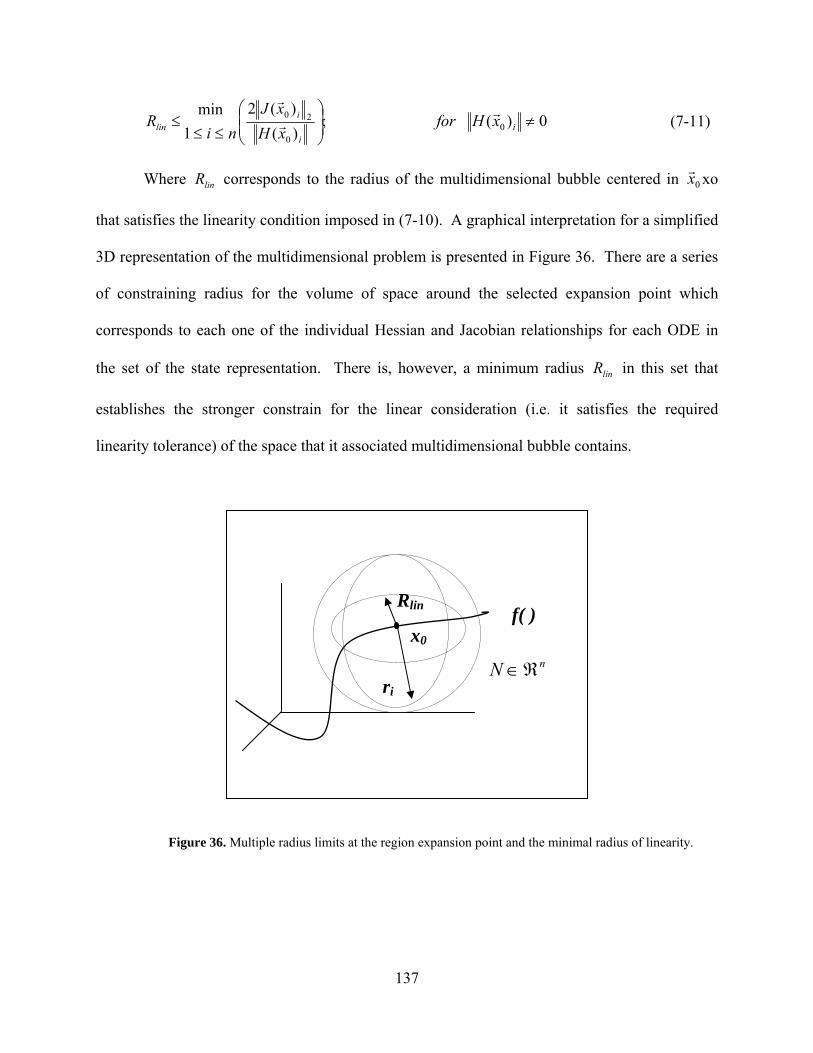
137
;)(
)(2
1
min
0
20
i
ilin xH
xJ
niR
0)( 0 ixHfor
(7-11)
Where linR corresponds to the radius of the multidimensional bubble centered in 0x
xo
that satisfies the linearity condition imposed in (7-10). A graphical interpretation for a simplified
3D representation of the multidimensional problem is presented in Figure 36. There are a series
of constraining radius for the volume of space around the selected expansion point which
corresponds to each one of the individual Hessian and Jacobian relationships for each ODE in
the set of the state representation. There is, however, a minimum radius linR in this set that
establishes the stronger constrain for the linear consideration (i.e. it satisfies the required
linearity tolerance) of the space that it associated multidimensional bubble contains.
Figure 36. Multiple radius limits at the region expansion point and the minimal radius of linearity.
nN
x0
Rlin
ri
f( )
138
7.3.1.3 Radius of linearization defined in the reduced state-space ( pZ )
The previous approach gives us a limit for the extension of a quasi-linear region i ( linR in Figure
36) which can be used as the basis for an optimization algorithm for the selection of expansion
points in the TPWL methodology. However, as it can be deduced from the expression in (7-9),
this procedure is of )(nO computational complexity which can be considered costly given the
very large dimension of the problem that is being addressed ( nN ).
To overcome this limitation we show in this section that the preceding result can also be
extended to the much smaller state-space of the final model ( pZ , where: np ). Obtaining
a linearity limit for the quasi-linear region in the target state-space eliminates the previous
computational burden since the new cost is now in the order of the reduced state size (i.e.,
)( pO ).
Let us approximate the state-representation of the nonlinear system in (7-1) replacing the
nonlinear function )(xf
with its Taylor expansion in two terms (i.e., including the quadratic
term, Hessian) as presented in (7-2):
xCy
tBuxxxxxHxxxJxfxET
)()())((2/1))(()( 000000 (7-12)
After some mathematical manipulation a simplified version of this expression where a
constant source 0G (i.e., ))(()( 00000 xxxHxfG
, nG 0 ) is added to account for the non-
state dependent terms (i.e., set up value for the Taylor expansion at 0x ):
xCy
tBuGxxxHxxJxET
)())((2/1)( 000 (7-13)
139
This expression in the state-space nN is directly related to the expression for the
linearity limit obtained in (7-11) which defines the reach of the region centered at 0x (i.e.,
multidimensional bubble of space defining the quasi-linear region).
In order to project the previous expression in a reduced state-space defined by the
projection base nxpV we follow a similar development as shown by Philips in [60]. For the
reduction of the higher terms the same projection base is used in multiple products:
Using the change of state Vzx into (7-13) gives us the following development:
zVCy
tBuUGUzVzVxHUzVxJUzEVUT
TTTTT
)())((2/1)( 000 (7-14)
Replacing the projected elements for the corresponding notation in the reduced
space pZ , and using Kronecker product property over )( zVzV
give us:
zCy
tuBGzzVVxHUzxJzET
r
rrT
rr
)())()((2/1)( 00 (7-15)
In the previous expression the term that operates over the quadratic
product )( zz
corresponds to the Hessian of the Taylor expansion defined now in the reduced
state-space Z.
zCy
tuBGzzxHzxJzET
r
rrrrr
)())((2/1)( 00 where: 2
)(
)(
0
0
pxpr
pxpr
xH
xJ
(7-16)
Because the expression (7-16) exactly matches in structure the expression in (7-13) but in
the reduced state-space Z, the previous result for defining the limit for the linearity of the region
can be then applied directly to this new formulation:
;)(
)(2
1
min
0
20
ir
ir
rlin xH
xJ
piR
0)( 0 ir xHfor
(7-17)
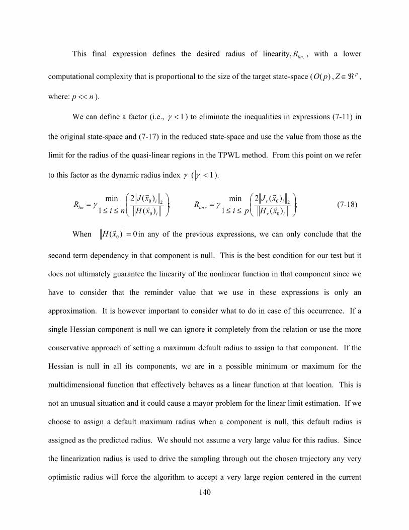
140
This final expression defines the desired radius of linearity,rlinR , with a lower
computational complexity that is proportional to the size of the target state-space ( )( pO , pZ ,
where: np ).
We can define a factor (i.e., 1 ) to eliminate the inequalities in expressions (7-11) in
the original state-space and (7-17) in the reduced state-space and use the value from those as the
limit for the radius of the quasi-linear regions in the TPWL method. From this point on we refer
to this factor as the dynamic radius index ( 1 ).
;)(
)(2
1
min
0
20
i
ilin xH
xJ
niR
;)(
)(2
1
min
0
20
ir
ir
rlin xH
xJ
piR
(7-18)
When 0)( 0 xH
in any of the previous expressions, we can only conclude that the
second term dependency in that component is null. This is the best condition for our test but it
does not ultimately guarantee the linearity of the nonlinear function in that component since we
have to consider that the reminder value that we use in these expressions is only an
approximation. It is however important to consider what to do in case of this occurrence. If a
single Hessian component is null we can ignore it completely from the relation or use the more
conservative approach of setting a maximum default radius to assign to that component. If the
Hessian is null in all its components, we are in a possible minimum or maximum for the
multidimensional function that effectively behaves as a linear function at that location. This is
not an unusual situation and it could cause a mayor problem for the linear limit estimation. If we
choose to assign a default maximum radius when a component is null, this default radius is
assigned as the predicted radius. We should not assume a very large value for this radius. Since
the linearization radius is used to drive the sampling through out the chosen trajectory any very
optimistic radius will force the algorithm to accept a very large region centered in the current
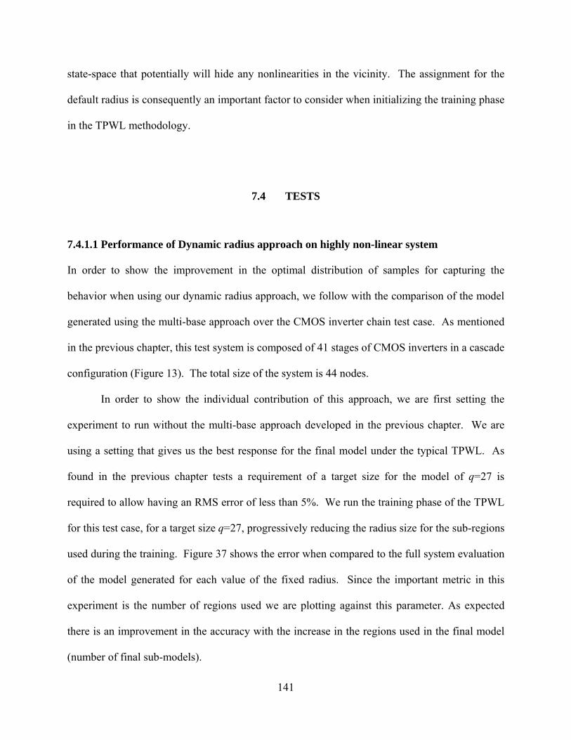
141
state-space that potentially will hide any nonlinearities in the vicinity. The assignment for the
default radius is consequently an important factor to consider when initializing the training phase
in the TPWL methodology.
7.4 TESTS
7.4.1.1 Performance of Dynamic radius approach on highly non-linear system
In order to show the improvement in the optimal distribution of samples for capturing the
behavior when using our dynamic radius approach, we follow with the comparison of the model
generated using the multi-base approach over the CMOS inverter chain test case. As mentioned
in the previous chapter, this test system is composed of 41 stages of CMOS inverters in a cascade
configuration (Figure 13). The total size of the system is 44 nodes.
In order to show the individual contribution of this approach, we are first setting the
experiment to run without the multi-base approach developed in the previous chapter. We are
using a setting that gives us the best response for the final model under the typical TPWL. As
found in the previous chapter tests a requirement of a target size for the model of q=27 is
required to allow having an RMS error of less than 5%. We run the training phase of the TPWL
for this test case, for a target size q=27, progressively reducing the radius size for the sub-regions
used during the training. Figure 37 shows the error when compared to the full system evaluation
of the model generated for each value of the fixed radius. Since the important metric in this
experiment is the number of regions used we are plotting against this parameter. As expected
there is an improvement in the accuracy with the increase in the regions used in the final model
(number of final sub-models).

142
CMOS Inverter Chain 44 Nodes, Radius Sweep, q=27
0
2
4
6
8
10
12
55 75 95 115 135No. Regions
Avg Error %RMS Error %Max RMS Error %Max Output (Volts)
Figure 37. TPWL Fixed radius approach: Error vs. No of regions for a requested size q=27.
In order to evaluate the effect of the dynamic radius metric on the methodology, the
previous test is repeated but using now a sweep in the dynamic radius index on expression 7-
18 from 0.5 to 0.1 which give us and effective sweep in the number of regions found from 51 to
85. The accuracy of the generated models is shown in Figure 38.
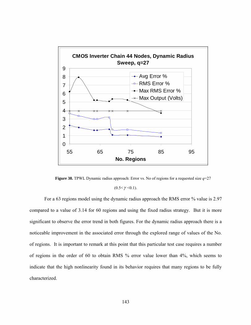
143
CMOS Inverter Chain 44 Nodes, Dynamic Radius Sweep, q=27
0
1
2
3
4
5
6
7
8
9
55 65 75 85 95No. Regions
Avg Error %
RMS Error %Max RMS Error %Max Output (Volts)
Figure 38. TPWL Dynamic radius approach: Error vs. No of regions for a requested size q=27
(0.5< <0.1).
For a 63 regions model using the dynamic radius approach the RMS error % value is 2.97
compared to a value of 3.14 for 60 regions and using the fixed radius strategy. But it is more
significant to observe the error trend in both figures. For the dynamic radius approach there is a
noticeable improvement in the associated error through the explored range of values of the No.
of regions. It is important to remark at this point that this particular test case requires a number
of regions in the order of 60 to obtain RMS % error value lower than 4%, which seems to
indicate that the high nonlinearity found in its behavior requires that many regions to be fully
characterized.

144
CMOS Inverter Chain 44 Nodes, Dynamic Radius Sweep, q=27 (+ Multi-projection base)
0
1
2
3
4
5
6
7
8
9
55 65 75 85 95 105No. Regions
Avg Error %RMS Error %Max RMS Error %Max Output (Volts)
Figure 39. TPWL Dynamic radius approach: Error vs. No of regions for a requested size q=27 (0.5< <0.1) but
with the multi-projection base option enable.
Figure 39 shows the response of the test when in addition to using the dynamic radius
approach we also enable the multi-projection base strategy. In terms of % RMS error this option
offers the best result. This result is expected since both techniques are aimed to reduce specific
factors that contribute to error in this methodology. However, we need to mention that this is not
the best implementation possible. As seen in the previous chapter there is a minimal realization
found when using a size q=6 in the multi-projection base strategy. A possible application of
145
these strategies into an automatic implementation of a TPWL model will require a valid
alternative to judge the merit of the model without doing a full system evaluation.
7.4.1.2 Performance of Dynamic radius approach on weakly non-linear system
For this test we are interested in to find if the use of the dynamic radius metric give the user and
efficient alternative for choosing a suitable size for the regions in the training process. This
could be used as the starting mechanism for an automatic region size selection for the algorithm
with minimal if any user intervention.
Figure 40.TPWL training phase for a RC nonlinear ladder, N = 400 nodes using dynamic radius approach.
We start with the RC nonlinear ladder circuit (shown in Figure 12), 400 nodes that we
have used in previous chapters. Through TPWL, we obtain a reduced model for this system for a
reduced size of 20 states (q=20). TPWL is using the original fix radius defined as a ratio of the
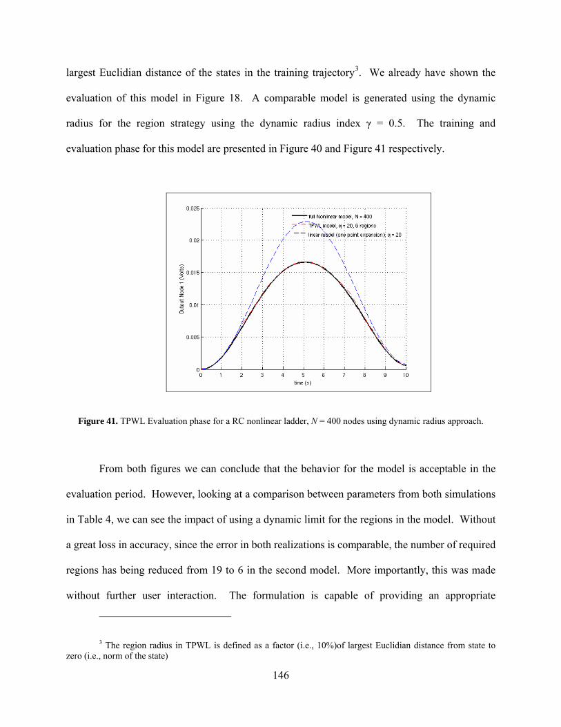
146
largest Euclidian distance of the states in the training trajectory3. We already have shown the
evaluation of this model in Figure 18. A comparable model is generated using the dynamic
radius for the region strategy using the dynamic radius index γ = 0.5. The training and
evaluation phase for this model are presented in Figure 40 and Figure 41 respectively.
Figure 41. TPWL Evaluation phase for a RC nonlinear ladder, N = 400 nodes using dynamic radius approach.
From both figures we can conclude that the behavior for the model is acceptable in the
evaluation period. However, looking at a comparison between parameters from both simulations
in Table 4, we can see the impact of using a dynamic limit for the regions in the model. Without
a great loss in accuracy, since the error in both realizations is comparable, the number of required
regions has being reduced from 19 to 6 in the second model. More importantly, this was made
without further user interaction. The formulation is capable of providing an appropriate
3 The region radius in TPWL is defined as a factor (i.e., 10%)of largest Euclidian distance from state to zero (i.e., norm of the state)

147
distribution of samples in the training trajectory that is completely dependent on the nature of the
system and that does not require cumbersome and successive adjustment from the user.
Table 4. Comparison of parameters for the TPWL generated model using fixed radius and dynamic radius for a RC
nonlinear ladder, N = 400 nodes, shown in Figure 12.
It is important to mention that in a homogeneous distribution, where the nonlinearities are
concentrated and of exponential nature, it is not surprising to find that the constraints from the
estimator evaluation are few and the same. Consequently the permissible radius for the entire
state-space is constant and equal to the value suggested in Table 4 (after being affected by our
chosen dynamic radius index).
7.4.1.3 Computational cost of the Dynamic radius strategy
As in the previous case the cost associated with this addition to the TPWL methodology
is added entirely to the training phase. The evaluation phase it is not affected directly by this
modification since we are not using this metric to affect the weight computation on the final
model (this is a future consideration for this methodology).
Region Radius No. Regions Avg. Output Error (%)
Fixed Radius TPWL 0.00484 19 0.32
Dynamic Radius
(Hessian based), γ = 0.5
0.017678 6 0.7

148
The cost associated with the Hessian computation could be relatively expensive since the
order of operations related with this figure is on the order of O(N3), where N is the size of the test
system, if we are not considering any optimization in place (worst case). Because of this, we
have tried to minimize the number of operations involved in the evaluation of the expression
used to estimate the dynamic radius index (7-18). Further optimization in speed or memory
requirements could be added such as considering the matrix’s sparsity to simplify the memory
requirements in this computation. Nevertheless, we could conclude acknowledging a possible
high cost depending on the size of the system under study.
We should, however, consider that the training phase is a one time cost. Consequently,
the speed up achieved through the use of MOR for the simulation of nonlinear systems can be
considered to be dominated by the evaluation cost if the final model can be used many times
during its life time. In traditional linear model order reduction the speed up is widely assumed
only related with the dimensional size for the reduced model.
For the system considered under study we do not see an impact in the training time in the
data shown in Figure 42 and Figure 43 for the case of using the fixed radius approach and the
dynamic radius strategy. As in the previous chapter, the overhead cost of the entire training
algorithm is much more significant to the extra cost added by the computation of the Hessian and
the operations related to it. This does not have to be the case for very large systems where the
high cost of the Hessian will be the dominant factor.

149
CMOS Inverter Chain 44 Nodes, Radius Sweep, q=27
0
10
20
30
40
50
60
70
80
90
55 75 95 115 135
q
Training Duration (s)
Evaluation Duration (s)
Figure 42. TPWL Fixed radius approach: Timing on training and evaluation phase.
CMOS Inverter Chain 44 Nodes, Dynamic Radius Sweep, q=27
0
10
20
30
40
50
60
70
80
90
55 65 75 85 95
q
Training Duration (s)
Evaluation Duration (s)
Figure 43. TPWL Dynamic radius approach: Timing on training and evaluation phase.

150
It is also interesting to note that there is an increase in the evaluation time that is
expected, in both situations, in Figure 42 and Figure 43 since the number of regions to evaluate
is increasing. The weight function operates over a larger set and this adds to the cost of the
evaluation process. As mentioned in Chapter 5, the cost associate with the weight evaluation for
the combination of the sub regions can be estimated to be on the order of O(q2s) where q is the
size of the model and s is the number of regions used in the model. Since the q size of the model
is maintained constant for this set of tests the evaluation time is now directly depending on the
number of regions (sub-models) used for the implementation. As shown in both figures
increasing the number of regions can undermine any gain obtained by the reduction in size
achieved.
7.5 SUMMARY
In this chapter we have introduced a new mechanism to optimize the selection of the points of
the original state-space of the nonlinear system that are going to be used as expansion points to
generate the linearized models that after reduction would form the TPWL model of the system.
This technique is based on deriving a figure of merit for the degree of linearization of the quasi-
linear region from the Hessian information of the system at that location.
After introducing the need for this proposed optimization in TPWL, we describe the
errors that affect the compact model produced by this methodology. We discussed that a better
approach to the simple but inefficient use of a uniform radius is to use a dynamic estimator for
the allowed size for the volume of the quasi-linear regions in the model. We then developed an

151
expression for the estimation of the radius of these linear regions which is based on the Lagrange
Remainder concept and the information carried out by the Hessian of the approximation.
A series of tests were presented to verify the performance of the proposed metric.
Through these tests, we have shown that this technique provides a mechanism to optimally locate
the sampling points describing the behavior of the system through the map of its state-space. It
was shown that the dynamic radius approach gives us a smaller overall error in the generated
model when compared to the fixed radius strategy. Furthermore, the combination of the multi-
domain strategy discussed in the previous chapter and this new approach for adjustable radius of
the regions of expansion combine to offer the best accuracy when compared to each individually
or to the original TPWL method. There is no a significant advantage when dealing with a
weekly nonlinear case as the non-linear ladder, since because of the homogeneous structure of
the system the suggested radius is of the same value. However, the dynamic radius metric still
offers a suggested value that produces an acceptable accuracy in the generated model.
Table 5. TPWL Dynamic radius approach: CMOS Inverter Chain 44 nodes. Speed up vs. Error for different No. of
regions used.
No. Regions Speed Up Avg. Error % RMS Error %
51 2.254518 2.38352 4.13625 53 2.249869 2.31056 3.9006 55 2.05314 2.21877 3.64343 58 2.036235 1.97115 3.3477 63 1.760988 1.63281 2.9784 64 1.433531 1.63229 2.97777 68 1.690951 1.7435 3.15425 69 1.416156 1.09219 1.73073 74 1.156103 1.06228 1.71757

152
Finally, we discuss the computational cost associated with the addition of the dynamic
radius strategy to the TPWL methodology. The cost is directly related to the cost of the Hessian
evaluation during the training phase and it could become expensive if the N of the system is very
large. However, we have to emphasize that the cost of the training phase is the natural penalty
for these types of methodologies. In Table 5, for the CMOS Inverter chain (44 nodes) system we
show the speed up in relation with the full evaluation of the system when adjusting the dynamic
radius index to obtain different number of regions in the final mode. Considering that this
particular selection for the size of the model (q =27) give us just a small gain in evaluation time
(the purpose of this selection being a successful model for single base and multi-base
approaches), we can however see the impact of the increasing number of regions in the speed-up
and accuracy of the model. As previously mentioned the gain in computation speed achieved by
the reduction itself (44 27) will be quickly compromised by an increase in the number of
regions. So a compromise between this to parameters is required for an effective final model.
In summary, the proposed dynamic radius strategy can both be used to reduce the number
of points and consequently the number of linear sub-models required to achieve a specified level
of accuracy in the final behavior of the reduced system or to increase the level of accuracy for a
fixed number of allowed regions of operation.

153
8.0 SUMMARY AND CONCLUSIONS
In this chapter we initially enumerate the main results obtained through this dissertation.
Following with the conclusions that we arrived by all the analysis and studies from previous
chapters.
8.1 CONTRIBUTIONS
The major contributions of this dissertation are the followings:
To our knowledge we are the first to introduce the use of the Hessian of the nonlinear
function in a nonlinear large system representation as the basis to generate a metric that can
be used to judge the quality of the linearity in a quasi-linear region of those found in a
trajectory based piece-wise linear methodology. We avoid the computational cost of finding
the exact maximum value of the Hessian and its location in the vicinity of the linearization
point establishing instead an approximated value at this location. The metric is based on the
use of the Lagrange remainder of the second order for the Taylor series expansion of the
multidimensional function at the sampling location. The importance of this proposal is the
use of this metric for the optimization of the location of sampling points in the chosen
trajectories and as a consequence in the volume of space under study.

154
We use multiple projection bases in the reduction process together with the optimization of
the location of samples in the state-space of the nonlinear system under study to improve the
accuracy of the generated model while conserving its size to a minimum. Tiwary and
Rutenbar [43] also use the concept of multi-projection base for the improvement in the model
generation. However, the mayor difference in both approaches is the progressive merging of
individual bases in our case and the use of an orthogonalization algorithm to accomplish this.
Our approach iteratively update the aggregated projection base each time a new projection
base is generated using an orthogonalization procedure based on the Gram-Schmidt algorithm,
while Tiwary adds each base as a whole leaving the pruning as the last stage of the process.
While the final result of both methods is equivalent we believe that an iterative approach is
more efficient in terms of memory use while paying a small cost per orthogonalization per
region. This cost is compensated by the low cost of the truncation of the final projection
base. Progressive orthogonalization offers a combined projection base that is already free of
common subspaces. Consequently the cost of the final SVD operation for the truncation to
the desired size is smaller. It is important to remark that Tiwary’s approach does not grow
alarmingly in size since he is already selecting a small number of bases for the merging using
his nearest neighbor-clustering approach.
We introduce the concept of hierarchical reduction for a large nonlinear system realization to
divide and simplify the overall reduction process. The use of a block projection approach
allows us to identify linear and nonlinear blocks in the original representation that can be
treated separately to reduce the overall effort in the reduction task.
Over the past years several groups have developed and enhanced the idea of using
trajectory piecewise linear models for non-linear model order reduction. Our contributions and

155
their relation to the work of M. Rewienski et al, J. Roychowdhury et al, and S. K. Tiwary and R.
A. Rutenbar, are summarized in Table 6. There is a clear similarity with the work of S. K.
Tiwary but our strategies although when offering similar solutions are obtained by different
approaches.
Table 6. Contributions and relationhip to significant research in the area.
Order of
sub-models
Sub-region volume Hierarchy Support Multiple
Projection Bases
M. Rewienski et al
[3][42]
Linear Fixed No No
J. Roychowdhury
et al [4][41][59]
High Order
(+2nd / 3rd)
Fixed No No
S. K. Tiwary,
R. A. Rutenbar
[43][44][45]
Linear Computed using nearest
neighbor approach
(Training and Evaluation
Phase)
Support limited
hierarchy
Yes
J. A. Martinez Linear Computed using the
Hessian (Training Phase)
- Chapter 7 -
Theoretical proposal
- Chapter 3 -
Yes
- Chapter 6 -
8.2 SUMMARY
In this dissertation we have discussed the need for improvements over current approaches used
for the model order reduction of very large nonlinear systems.
In Chapter 2, we presented and discussed ideas currently used for the reduction of large
nonlinear system representations and the difficulties and limitations found in each one of these

156
techniques. In doing so, we establish the need for improvement upon the current alternatives for
the generation of compact models for large nonlinear dynamic systems.
In Chapter 3, we proposed to use a hierarchical approach for the reduction process of a
very large nonlinear system. We show how using a block projection base strategy gives us the
ability of detection of linear/nonlinear sections in the original system representation that can then
be separately treated simplifying the overall reduction task.
In Chapter 4, we presented our MATLAB based analog solver platform. We described
the simulation strategy used in its development, and its more important components. This set of
programs that allow the simulation of compatible circuit descriptions (i.e., SPICE netlist) was
developed to support our research in nonlinear circuit simulation and model order reduction. We
showed a performance evaluation between both this novel platform and a commercial well
known circuit solver, HSPICE.
In Chapter 5, we presented the trajectory based piecewise-linear technique for the model
order reduction of large nonlinear systems which we used as the starting point for the
development of our methodology. After initially describing the algorithm and the details
surrounding the ensemble final model, we then presented its advantages and limitations.
In Chapter 6, we proposed the use of a multi-projection based approach strategy to
improve the accuracy of nonlinear model order reduction. We initially presented a detailed
description of the sources of error in a piece-wise based reduction methodology with special
emphasis in the case of loss of accuracy as a consequence of using a single base generated from a
single state point. We proposed an algorithm to merge the information from multiple projection
bases obtained from an equal number of sampling points to generate a more suitable base for the
volume of space considered. We then followed with a strategy to accommodate this extended
157
projection base into the piecewise-linear methodology. We evaluated the performance of the
model order reduction technique with the addition of these changes.
Finally, in Chapter 7, we introduced a novel mechanism to generate a linearization metric
that can be used to optimize the location of the states for the linear approximations in the
reduction process. We discussed how the performance of the resulting compact model is highly
dependent on the state-space location for the linear approximations. We introduced a radius
metric that is derived from error bound estimation at the sampling location using the Hessian of
the system and considering the Lagrange remainder of the linear approximation. We verified the
improvement in performance of the model order reduction technique with the addition of this
optimization strategy in terms of the number of samples required to achieve a specified level of
accuracy in the final compact model.
8.3 CONCLUSIONS
A trajectory based model order reduction methodology is a practical solution to the problem of
order reduction of very large general nonlinear systems. However, in its present form there is a
series of drawbacks that needs to be addressed in order to make it a reliable approach.
Through this dissertation we have analyzed the basic TPWL methodology and showed its
limitations. Several improvements have been proposed that allow one to overcome some of
these original limitations.
The method has a strong dependency on the selected locations in the state-space where
the snapshots of the system are taken to construct the final linear combined model. This is
consequence of the very simple weight function used in the technique. An empirical scalar-

158
switching weight function is a very restrictive element that does not contain any information
from the nature of the nonlinear space it is intended to help to model. Since the function is
Omni-directional in its behavior and its shape is basically selected before hand, the nature of the
interpolation between sampling points to estimate the real nature of the space is a guess at best.
We have introduced two strategies to alleviate this dependency. First, the use of a multi-
projection base strategy that allows us to reduce the error in the evaluation as a consequence of a
poor projection base estimation. The significance of this is that any amount of error introduced
into the compact model evaluation is potentially a cause for an early drift in the response. TPWL
does not have any correction mechanism to mitigate errors in the evaluation and the sensitivity of
the weight function only serves to magnify this problem. Second, the use of a Hessian based
strategy for the optimization on the location of the sampling points. Having a better sampling
distribution increases the accuracy and minimizes the likelihood of errors since there will be a
denser distribution in those regions of the space that demands large changes in the behavior of
the function.
The accuracy and applicability of a compact model from this or similar techniques
depends on how well the state-space of the function has been sampled. This translates in
practical terms in a large set of snapshots generated from an equally large set of training
trajectories. The use of an optimization algorithm for the selection of these samples even when
initially computationally costly serves to obtain a set of smaller size for the same expected level
of accuracy.
We have also discussed how to increase the volume of the state-space that the problem
produces as an unwanted consequence the increase in size of the required projection base to
capture all the relevant behaviors in the system. Eventually, the larger required size for the

159
resulting realization negates the benefits of model reduction itself, since the state-space for the
model could be on the order of the original problem size. A solution for this situation is the use
of a hierarchical approach as previously discussed for the reduction methodology. Separating the
realization by blocks and generating compact models for these sections is a viable alternative that
conserves the benefits of MOR while dealing with long domain evaluations.
We believe that further work in this direction is needed to achieve a reduction
methodology that can produce compact models that are computationally efficient and robust in
their performance.
160
9.0 FUTURE WORK
At the end of this work we are faced with an interesting avenue of possibilities to pursue further
studies in this field. Nonlinear model order reduction is a very young and active field with a
potential for significant influence in other areas of knowledge. Specifically, any potential
development here could be immediately applied to alleviate the increasing appetite for
computational capacity in speed and memory for the simulation of the new large VLSI designs
that deal with increasing complexity of interconnections at the submicron level. We now
enumerate those ideas that can be further developed based on the results of this work:
A limitation on the degree of accuracy achievable with a trajectory based model order
reduction technique is the scalar nature of the weight function normally used. Since this
function is doing a scalar weight over all the dimensions in the reduced state-space for
the compact realization this translates into an omni-directional contribution allocation.
This is a very restrictive condition that affects how well a matching per state can be
achieved. However, the advantage of this scalar selection is its computational simplicity.
Since it is a scalar factor affecting the whole representation it offers a lower
computational demand in the analog solver used for the evaluation of the model. This is
especially true when compared with the extreme alternative. To achieve the maximum
possible matching in the set of linear snapshots and consequently the more accurate
multidimensional fitting, a multi-dimensional weight matrix should be considered. In

161
this situation, every single dimensional contribution for the reduced model equivalent of
the transfer function its matched by a single function. The result is a weight function of
size qxq , where q is the order of the reduced system. This is equivalent to an adjustable
transformation matrix of the same range.
Even with the associated high computational demand that this type of weight
selection imposes in the analog solver during evaluation the total control over all the
available degrees of freedom in the representation offers it the best possible matching in
between the set of snapshots taken as samples for the desired multidimensional function.
This is exactly equivalent to multidimensional curve fitting for the unknown nonlinear
function in the reduced state-space.
A compromise can be obtained between degrees of freedom against computational
complexity if the weight matrix is allowed to operate over a reduced set of the
dimensions. This screening can be achieved through a filter process involving these
multidimensional samples, where the locations that show larger variability are retained
according to some predefined threshold. This more elaborated weight function or
envelope should offer a better performance when compared to the single scalar type.
We have proposed and show how using the Hessian of the system under analysis as a
metric to judge the optimal size for the linear sub-region in the TPWL methodology. This
approach improves the sample distribution in the state-space from the training process,
and consequently improves the performance of the model since a proper dynamic
granularity of the state-space is produced. However, this metric could still be used for an
improved merger of the sub models during the evaluation phase. A snapshot can be
defined as composed of a reduced linear sub-model, the expansion point (pivot) and the

162
radius associated with this region (obtained when using the dynamic radius approach).
The weight function can then be adjusted to also include the information related to the
size of the bubble associated with each sub-model when doing the average.
163
APPENDIX A
MODEL ORDER REDUCTION RELATED CONCEPTS
In this section we are including a few concepts and techniques that are needed for the completion
of this document. The reader is welcomed to expand this information through the provided
references.
A.1 STATE REPRESENTATION FOR A DYNAMIC SYSTEM
This is a mathematical description for a dynamic system where the relation between the outputs
and the inputs of a system is presented as a function of a state vector x(t)[81]. The system can
then be represented as a set of first order differential equations in terms of this state vector. The
output from the system is obtained through an algebraic equation in terms of this state vector.
A linear state representation of a multiple-input multiple-output (MIMO) linear system
has the following standard form:
Cxy
BuAxxE
,
(A-1)
Where nx represents the state vector, mu is the vector of inputs to the system
and py is its response. nxnE is known as the mass, memory or storage matrix, nxnA

164
is known as the transition or open-loop dynamic matrix, nxmB is known as the input
connectivity or control distribution matrix, and pxnC is called the output connectivity or
sensor calibration matrix.
In a wide range of systems it is very easy to construct a model using this representation
and to choose as a state vector a set of physical variables of the problem (e.g., Kirchhoff’s
Current Law (KCL) and Kirchhoff’s Voltage Law (KVL) state definitions, vector of position in a
multi-body dynamic system).
This model became widely used after the popularity of Kalman’s work [10][11] for
prediction and control of linear systems. Some of the advantages of this formulation are the
simplification of the representation, stability analysis, and control mechanism for MIMO
problems.
A.2 THE ORTHOGONALIZATION GRAM-SCHMIDT ALGORITHM
This process is used to obtain a set of orthogonal vectors },...,,{ 21 nvvv from a finite set of
linearly independent vectors },...,,{ 21 nuuu defined both in the same Euclidian subspace nS .
The orthogonality property is defined using an inner product, commonly in the Euclidian
space n .
The working of this method can be understood from a geometric point of view as
follows:
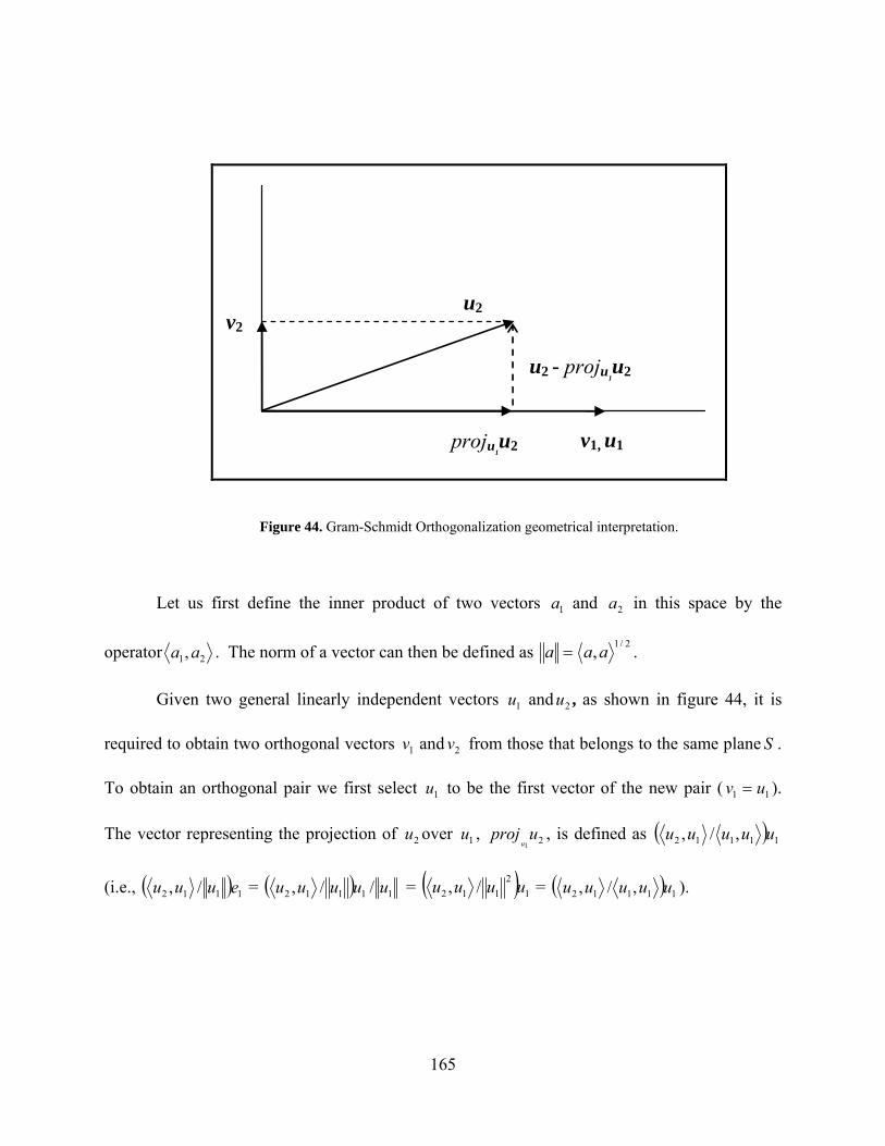
165
v1, u1
v2 u2
proju1u2
u2 - proju1u2
Figure 44. Gram-Schmidt Orthogonalization geometrical interpretation.
Let us first define the inner product of two vectors 1a and 2a in this space by the
operator 21, aa . The norm of a vector can then be defined as 2/1
,aaa .
Given two general linearly independent vectors 1u and 2u , as shown in figure 44, it is
required to obtain two orthogonal vectors 1v and 2v from those that belongs to the same plane S .
To obtain an orthogonal pair we first select 1u to be the first vector of the new pair ( 11 uv ).
The vector representing the projection of 2u over 1u , 21uproj
u, is defined as 11112 ,/, uuuuu
(i.e., 1112 /, euuu = 11112 //, uuuuu = 1
2
112 /, uuuu = 11112 ,/, uuuuu ).
166
This component is then geometrically subtracted from 2u which gives as a result a new
vector 2221uprojuv
u , which is itself orthogonal to 1v . The orthogonal pair 21,vv could,
additionally, be normalized to generate an orthonormal base 21,ee for the subspace S (i.e.
2/1
1111 ,/ vvve ,2/1
2222 ,/ vvve ).
Extending this procedure to an iterative algorithm for a number of n vectors gives us the
general form for this method [73]:
2/1
1
1 , ,
,
,
jj
jj
k
jj
jj
jk
kkvv
vev
vv
vuuv
(A-2)
A.3 KRYLOV SUBSPACE METHODS
Most of the success of model order reduction for large linear systems came from the
development of efficient projection algorithms based on KRYLOV subspaces. KRYLOV subspace
methods are one of the more successful tools available in numerical linear algebra. Before going
into specific techniques such as the ARNOLDI algorithm [54] and LANCZOS projection [26] let us
describe what a KRYLOV subspace is and why it is so useful for the solution of this kind of
problem.
When having to solve a linear problem Ax = b, where the matrix nxnA is non-singular,
sparse and of a very large size, the solution using Gaussian elimination would be very
unpractical if the size of the system n is a very large number. There are also problems where A is
not given explicitly but as a matrix-vector product once the vector is supplied. The KRYLOV
subspace method establishes that the solution of this system is in a subspace of order q which

167
also corresponds to the rank of A. This subspace rank can be very small when compared to the
real size n of A which reduces the time to find the solution. The desired subspace is reached
through the expansion of successive matrix products of the matrix A and a starting vector c.
Each one of these vector products defines a vector of the KRYLOV subspace. The solution x for
the system can consequently be expressed as a linear combination of these components.
The number of these components or vector bases corresponds to k, the range of A. The
KRYLOV subspace is then defined as being spanned by these components also known as vectors
of the Krylov sequence:
,,...,,),( 1cAAccspancAK qq
Consequently, the solution x for the system can also be described as the linear
combination:
,,.., 1110 cAaAcacax q
q
It can be proved [20] that the solution to a nonsingular linear state-space representation
can be approximated to a representation contained in a KRYLOV subspace. This allows this
subspace to be used instead of the eigenvalue solutions to find a projection base to reduce the
state-space of the system representation. Even further, certain KRYLOV subspaces of a linear
dynamic system correspond to reduced projections that include the more important moments of
the expansion of the original system in the frequency domain around s=0. Consequently, not
only does the KRYLOV subspace technique give us a reduced state-space but it also corresponds
to the selection process of the more significant state components of the system. This explains the
popularity of Krylov subspace methods in MOR.
For a state-representation of a linear dynamic system such as (A-1) the two associated
KRYLOV subspaces corresponding to the moment matching condition are the input and the output

168
KRYLOV subspace, depending on the selection for the vector c. The input KRYLOV subspace is
obtained from spanning successive products of the inverse transfer matrix A-1 and the
connectivity vector A-1B associated with the input to the system, Kq(A-1, A-1B)= span{A-1B, A-2B,
A-qB}. The output KRYLOV subspace is, on the other hand, related to the spanning of successive
products of the inverse transposed transfer matrix A-T and the connectivity vector A-TCT
associated with the output from the system, Kq(A-T, A-TCT)= span{A-TCT, A-2TCT,…, A-qTCT}.
The selection of which KRYLOV subspace is used for the reduced representation of the
system gives origin to two different sets of projection algorithms: the one-sided KRYLOV and the
two-sided KRYLOV projection methods. The one-sided KRYLOV methods are the techniques that
use only one of the two important associated KRYLOV subspaces of a realization, input or output,
for the generation of a suitable projection base. If either one of these subspaces is used then the
algorithm can have a total of q moments matched. Where, q corresponds to the size of linearly
independent vectors for the KRYLOV subspace. If both KRYLOV subspaces are used then we are
using a projection method known as two-sided KRYLOV and the number of matched moments
increases to 2q. This number corresponds to the total number of linearly independent vectors
from both subspaces.
A.4 ARNOLDI BASED ALGORITHMS
In order to simplify the details of the following method let us define the following conventions:
V= [v1 v2 … vq] is a basis for the input KRYLOV subspace Kq(A-1, A-1B)= span{A-1B, A-2B,…, A-qB}
of the system description in (A-1), W= [w1 w2 … wq] corresponds to a basis for the output
KRYLOV subspace Kq(A-T, A-TCT)= span{ A-TCT, A-2TCT,…, A-qTCT } of the same representation.

169
A successful algorithm used, in its one-sided or two-sided versions, for obtaining the
projection base of a selected KRYLOV subspace for a state-space representation is the ARNOLDI
method [27][20]. In the classical version of the ARNOLDI algorithm an orthogonal base is
obtained for the selected KRYLOV subspace using modified GRAM-SCHMIDT orthogonalization
[72] over the KRYLOV vector columns.
Let us consider a KRYLOV subspace defined as κq(A, b) and use the ARNOLDI algorithm
to find the orthogonal basis V=[v1,v2,…,vq] that defines this subspace.
The algorithm extracts a set of vectors, columns of the basis V, which are orthogonal to
each other:
IVV ji
jivv T
jT
i
0
1
The algorithm principle is successively applying GRAM-SCHMIDT orthogonalization to
the set of basis matrix-vector products that defines a KRYLOV subspace. During each step i of
the algorithm a new normalized orthogonal vector is defined which is orthogonal to each of the
previous (i-1) vectors from previous cycles.
Let us describe the series of steps of the basic algorithm:
1. Initialization: Because we are defining an orthogonal set we can take any
vector of the set as the initial orthogonal basis. This initial vector is the
normalized initial matrix-vector product of the KRYLOV subspace b.
,b
bv 1
2. Next step: for i=2 to q,
Computing the next vector for the orthogonal set:
,Avv ii 1

170
A new vector that belongs to the KRYLOV subspace is the result of the product of its
defining Matrix A and the previous orthogonal vector. Remember at this point that
the KRYLOV subspace is composed of these successive matrix-vector products. Each
projection to A creates a new potentially linearly independent vector.
3. Orthogonalization: for j=1 to i-1,
Orthogonalization to previous components of the set using GRAM-SCHMIDT method:
,
,
jii
jT
i
hvvv
vvh
This is a very simple and straightforward methodology based on geometry. An
orthogonal new vector vj to a vector vi is generated when any projection over this
vector is subtracted.
If the resulting vector is zero (vi=0) this implies that the tested vector is a linear
combination of the previously defined orthogonal set and the suggested q size for the
KRYLOV subspace is over dimensioned. The algorithm should be terminated at this
point for a revaluation of the size of the KRYLOV subspace.
Finally a normalization of the orthogonal vector is applied:
,v
vv
i
ii
4. End: At the end of this q-1 steps the desired set of orthogonal vectors V,
defining the proposed KRYLOV subspace Kq(A, b), has been produced.
One popular option is the use of the input KRYLOV subspace in algorithms for MOR and
the ARNOLDI method to obtain the projection V for the system. To complete the projection
procedure the selection of the complementary basis for the output KRYLOV subspace could be
any arbitrary one that does not produce a singular reduced version of A. A good choice that is

171
widely accepted is using W = V. For the two-sided option of this method, the previous algorithm
is applied to both KRYLOV subspaces to obtain V and W respectively. This algorithm offers more
stability than an equivalent LANCZOS implementation with a reduced computational load.
A.5 LANCZOS BASED ALGORITHMS
In order to simplify the details of the following method let us define the following conventions:
V= [v1 v2 … vq] is a basis for the input KRYLOV subspace Kq(A-1, A-1B)= span{A-1B, A-2B,…, A-qB}
of the system description in (A-1), W= [w1 w2 … wq] corresponds to a basis for the output
KRYLOV subspace Kq(A-T, A-TCT)= span{ A-TCT, A-2TCT,…, A-qTCT } of the same representation.
The LANCZOS method [24][26] is widely used for extracting the projection bases for the
KRYLOV subspaces of a state-space representation of a linear dynamic system. The LANCZOS
algorithm applied over the input and output KRYLOV subspaces provides as a result the desired V
and W basis. Biorthogonality is forced in between these two sets through their formation by the
algorithm as described in [74]:
,IVW T (A-3)
An additional result of the algorithm is a tridiagonal matrix T which is related to the
original system by:
,TAVW T (A-4)
Where T is a matrix of the following structure also known as tridiagonal:

172
qqqq
aa
u
aa
aa
T
1,
1,
2221
1211
00
00
00
Observing the equation (A-4), it is easy to realize that the matrix T corresponds to a
reduced projection of the matrix A of the original system to the reduced KRYLOV subspace of
order q.
It is important to make a remark at this point on the result of this algorithm when
compared to the ARNOLDI method. Where in the ARNOLDI method we are obtaining an
orthogonal projection base, which means that its columns are orthogonal to each other, in the
LANCZOS technique this is not the case. This method gives us projection bases for each KRYLOV
subspace that are biorthogonal to each other as defined in (A-3) but they are not composed of
orthogonal vector columns.
The main disadvantage in the LANCZOS based method is that there is an innate instability
as a result of its loss of orthogonality between the generated vectors. A common solution to this
problem is additional steps for the checking of orthogonality and re-orthogonalization if required
[82].
Let us use the LANCZOS algorithm presented in [49] to describe the main aspects of this
method. We are considering the two KRYLOV subspaces Kq(A, b) and Kq(AT, cT) from the system
under test. The following algorithm uses a modified GRAM-SCHMIDT technique:
1. Initialization: Because we are defining an orthogonal set we can take any
vector of the set as the initial orthogonal basis.

173
bc
cw,
bc
bbcsignv
T
T
1T
T
)(
1
2. Next step: for i=2 to q,
Computing the next vector for the orthogonal set:
,wAw,Avv iT
iii 11
As in the previous method each projection to A (and AT for the next KRYLOV
subspace) creates a new potentially linearly independent vector.
3. Orthogonalization: for j=1 to i-1,
Orthogonalization to previous components of the set using GRAM-SCHMIDT method:
,,
,,
j2iijT
i2
j1iijT
i1
whwwvwh
vhvvwvh
In this step the orthogonality is enforced between the actual vectors and the opposite
set of vectors. So vi is orthogonalized to each vector wj (1≤ j ≤ i-1) at this stage.
Finally, the magnitudes of the vectors are adjusted according to:
i
Ti
ii
iT
i
iiT
ii
wv
ww,
wv
vwvsignv
)(
4. End: At the end of these (q-1) steps the desired set of biorthogonal bases V, W
defining the proposed reduction has been produced.

174
APPENDIX B
MODIFIED NODAL ANALYSIS (MNA)
In this formulation a dynamic linear time invariant system can be completely defined as a set of
ordinary differential equations (ODEs) in terms of a set of variables that will constitute the state
of the system. This ODE set will relate the state of the system to its inputs using an invariant
parametric matrix description. Any additional variables in the system can be derived using a set
of algebraic expressions in terms of the state variables:
,BuRxxM (B-1)
,DuxLy T (B-2)
For a development of this expression the reader can explore the work presented in
[75][76] and [77]. This formulation is based in the application of the KCL (Kirchoff’s current
law) over the nodal representation of the circuit and the use of the state variable definition,
i
vx . In this state definition nv corresponds to the vector of voltage nodes in the
network and mi corresponds to a vector representing only the currents going through
inductors, and sources in the network. What is accomplished with this state definition is a
transformation from a second order ordinary differential equation problem (ODE) to a first order
175
differential equation, at the expense of increasing the range of the linear problem from n to
(n+m).
The y vector contains the desired variables to evaluate and the u vector represents the
excitation to the system. M corresponds to the memory matrix of the system (another name for it
is the susceptance matrix) and R is the conductance matrix for the system. The structure of the
memory elements M and passive elements R is:
0
0
0;
L
C; M
E
EGR T
(B-3)
nxnC is the capacitance and mxmL is the inductance matrices of the network.
nxnG represents the conductance elements of the network and mxmE is the incidence
matrix of i in every node. B and D represent node incidence matrices for the input sources of the
system. D is an incidence matrix that allows one to obtain the desired set of variables y from the
state variable vector x.
A very useful feature of this representation is that the relative inclusion of any discrete
element (i.e., R, C, L, and sources) can be expressed as a pattern or specific template. Each
element type can be described as a set of specific R, M and B matrices. This set, or template, can
then be used to introduce the element into the global MNA, requiring only its position in terms of
a nodal index. The following section describes the mapping of the different classes of elements
to the MNA representation.
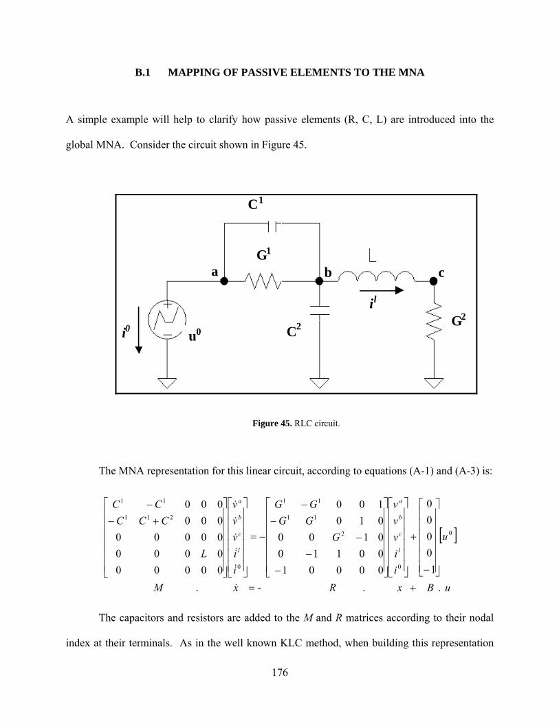
176
B.1 MAPPING OF PASSIVE ELEMENTS TO THE MNA
A simple example will help to clarify how passive elements (R, C, L) are introduced into the
global MNA. Consider the circuit shown in Figure 45.
il
a b c
i0 u0
C1
C2
G1
G2
Figure 45. RLC circuit.
The MNA representation for this linear circuit, according to equations (A-1) and (A-3) is:
uBxRxM
u
i
i
v
v
v
G
GG
GG
i
i
v
v
v
L
CCC
CC
l
c
b
a
l
c
b
a
. . - .
1
0
0
0
0
00001
00110
0100
010
100
00000
0000
00000
000
000
0
0
2
11
11
0
211
11
The capacitors and resistors are added to the M and R matrices according to their nodal
index at their terminals. As in the well known KLC method, when building this representation

177
the rows of the matrix equation correspond to the nodes in the circuit. Also, the columns in each
matrix have the same index order. As an example, the node a corresponds to the first row in the
matrix representation. The addition of all the capacitors connected to node a, C1, is the value to
put in location (a, a) of the matrix M. The rest of the elements on the row of M correspond to
capacitors connected between a and the rest of the nodes. In this example, the only element not
zero is (a, b) because C1 is also connected to this node. The value of these elements must be
negative because they corresponds to currents that are coming into the node a, which is opposite
to the accepted positive direction. Elements that are connected to ground on one end, such as G2
in the example, only have contribution to the non-ground node (c for G2). This is because the
reference node, ground, is not explicitly used, since all potentials are with reference to it.
The derivation of the templates for these elements is straightforward:
For a capacitor C:
0
0
B
R
v
v
CC
CCM
vv
b
a
ba
For a resistor R = 1/G:
0
0
B
v
v
GG
GGR
vv
M
b
a
ba
In these example templates the relative indices (va, vb) are added for clarification
purposes.
For the inductors however, a special consideration must be addressed. In the MNA
representation, each inductor in the network requires the state vector x to increase in size adding
the current through that element as a new variable. Consequently, the template for this element

178
must contain the new added variable, il, in addition to its location. This gives the following form
for inductor templates:
0
0 1 1
1 0 0
1 0 0
0 0
0 0 0
0 0 0
B
i
v
v
R
i
v
v
L
M
ivvivv
l
b
a
l
b
a
lbalba
Putting these templates together, using the common shared node indices (a, b, c), gives
the result shown in the final MNA representation.
B.2 MAPPING OF ACTIVE ELEMENTS INTO THE MNA
Active elements, such as independent sources, and dependent, controlled sources, require a
different treatment for the creation of the corresponding templates. To exemplify this procedure
the development of the template for a voltage source controlled by a voltage follows.
Figure 46 illustrates the general situation where a dependent voltage source is located
between the nodes a and b of a network. We assume that the value of this source is controlled by
the voltage difference between two different nodes of the circuit, k and l (vk-vl). The quantity g,
which is the transconductance between the nodes k-l and a-b, acts as the proportionality
parameter for the source. iab is the current through the controlled source measured from node a
to b.
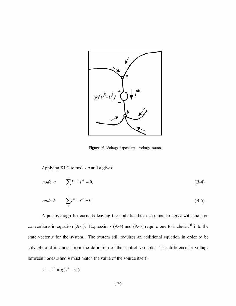
179
g(vk-vl)
b
iab
a
Figure 46. Voltage dependent – voltage source
Applying KLC to nodes a and b gives:
,0 abn
s
as iianode (B-4)
,0 abn
s
bs iibnode (B-5)
A positive sign for currents leaving the node has been assumed to agree with the sign
conventions in equation (A-1). Expressions (A-4) and (A-5) require one to include iab into the
state vector x for the system. The system still requires an additional equation in order to be
solvable and it comes from the definition of the control variable. The difference in voltage
between nodes a and b must match the value of the source itself:
),( lkba vvgvv

180
Arranging the terms according to their relative nodal position (assuming: a<b<k<l):
0 lkba gvgvvv (B-6)
Using equations (A-4), (A-5) and (A-6) in (A-1) allows one to extract a template for this
element of the form:
0
011
00000
00000
10000
10000
0
B
i
v
v
v
v
gg
RM
ivvvv
ab
l
k
b
a
ablkba
The symbolic location of the nodes is indicated in the matrix R for easy mapping to the
global MNA. Additionally, the global MNA must be increased in size to accommodate the
current through this element.

181
BIBLIOGRAPHY
[1] J.R. Phillips, “Projection-Based Approaches for Model Reduction of Weakly Nonlinear, Time-Varying Systems,” IEEE Trans. on Computer-Aided Design of Integrated Circuits and Systems,” Vol. 22, No. 2, pp. 171-187, February 2003.
[2] P. Li, T. Pileggi, “NORM: Compact Model Order Reduction of Weakly,” Proc. of 40th IEEE/ACM Design Automation Conference, DAC 2003, pp. 472-477, 2003.
[3] M. Rewienski and J. White, “A Trajectory Piecewise-Linear Approach to Model Order Reduction and Fast Simulation of Nonlinear Circuits and Micromachined Devices,” In Proc. ICCAD, Nov 2001.
[4] N. Dong and J. Roychowdhoury, “Piecewise Polynomial Nonlinear Model Order Reduction,” Proc. of 40th IEEE/ACM Design Automation Conference, DAC 2003, pp. 484 489, 2003.
[5] MATLAB, Mathworks, Inc.
[6] L. W. Nagel, "SPICE2: A computer Program to Simulate Semiconductor Circuits," ERL Memo. No. UCB/ERL, Vol. M75/520 (1975).
[7] R.W. Freund, “SPRIM: Structure-Preserving Reduced-Order Interconnect Macromodeling,” In Technical Digest of the 2004 IEEE/ACM Int. Conf. on Computer-Aided Design (ICCAD-2004), pp. 80-87, San Jose, California, 2004. IEEE Computer Society Press.
[8] HSPICE, Synopsis Inc.
[9] R. Genesio, M. Milanese, “A note on the derivation and use of reduced-order models. IEEE Trans. Automat. Contr., Vol. AC-21, pp.118-122, February 1976.
[10] R.E. Kalman, “Irreducible realizations and the degree of a rational matrix,” SIAM J. Appl. Math., Vol. 13, No. 2, pp. 520-544, 1965.
[11] R.E. Kalman, “Algebraic structure of finite dimensional dynamical systems,” Proc. Nat. Acad. Sci., U.S.A., Vol. 54, pp. 1503-1508, 1965.

182
[12] B.C. Moore, “Principal Component Analysis in Linear Systems: Controllability, Observability, and Model Reduction,” IEEE Transactions on Automatic Control, Vol. AC-26, No. 1, pp. 17-32, Feb. 1981.
[13] B.C. Moore, “Singular value analysis of linear systems, parts I, II,” Dep. Elec. Eng., Univ. Toronto, Toronto, Ont., Syst. Contr. Rep. 7801 and 7802, July 1978; also in Proc. IEEE Conf. Dec. Contr., pp. 66-73.
[14] P.T., Kabamba, “Balanced gains and their significance for L2 model reduction,” IEEE Trans. Automat. Contr., Vol. AC-30, No. 7, pp. 690-693, 1985.
[15] E.A., Jonckheere, L.M. Silverman. “A new set of invariants for linear systems – Applications to reduced-order compensator design.” IEEE Trans. Automat. Contr., Vol. AC-28, pp. 953-964, 1983.
[16] R. Ober, D. McFarlane, “Balanced Canonical Forms for Minimal Systems: A normalized Comprime Factor Approach,” Linear Algebra and its Applications, pp. 23-64, 1989.
[17] C.D. Yang, F.B. Yeh, “One-Step Extension Approach to Optimal Hankel-Norm Approximation and H∞ - optimization Problems,” IEEE Trans. Automat. Contr., Vol. AC-38, No. 6, pp.674-688, 1993.
[18] D.F. Enns, “Model Reduction with Balanced Realizations: An Error Bound and A Frequency weighted Generalization,” Proc. 23rd IEEE CDC, New York, 1984, pp. 127-132.
[19] Y. Chen and J. White, “A quadratic method for nonlinear model order reduction,” Tech. Proc. of the 2000 International Conference on Modeling and Simulation of Microsystems, Semiconductors, Sensors and Actuators, MSM 2000, San Diego, USA, pp. 477-480, March 2000.
[20] R.W. Freund, “Krylov subspace methods for reduced order modeling in circuit simulation,” Journal of Computational and Applied Mathematics. Vol. 123, pp. 395-421, 2000.
[21] R.W. Freund, “Passive Reduced-Order Modeling via Krylov Subspace Methods,” Proceedings of the 2000 IEEE International Symposium on Computer-Aided Control System Design, Anchorage, Alaska, USA, September 25-27, pp. 261-266, 2000.
[22] P. Feldmann, R.W., Freund, “Efficient linear circuit analysis by Padé approximation via the Lanczos process,” IEEE Trans. on CAD, vol. CAD-14, pp. 639-649, May 1995.
[23] R.W. Freund, P. Feldmann, “Efficient Small-signal Circuit Analysis and Sensitivity Computations with the PVL Algorithm,” IEEE/ACM International Conference on Computer-Aided Design, 1994, November 6-10, 1994, pp. 404-411.
[24] K. Gallivan, E. Grimme, P. Van Dooren, “A rational Lanczos algorithm for model reduction, Numerical Algorithm,” Vol. 12. No. 1, pp. 33-63, 1996.

183
[25] B. Salimbahrami, B; Lohmann, T. Bectold, J. G. Korvink, “Two-sided Arnoldi Algorithm and Its Application in Order Reduction of MEMs,” In Proceedings 4th MATHMOD, Vienna, pp. 1021-1028, Feb. 2003.
[26] Lanczos, C., “An Iteration method for the solution of the eigenvalue problem of linear differential and integral operators,” J. Res. Nat. Bureau Stan., Vol. 45, pp. 255-282, 1950.
[27] W.E. Arnoldi, “The principle of minimized iterations in solution of the matrix eigenvalue problem,” Quarrt., Appl. Math., Vol. 9, pp. 17-29, 1951.
[28] G.A. Baker, Jr. P. Graves-Morris, Padé Approximants, Part I: Basic Theory, Reading, MA: Addison-Wesley, 1981.
[29] P. Feldmann, R.W., Freund, “Efficient linear circuit analysis by Padé approximation via the Lanczos process,” IEEE Trans. on CAD, vol. CAD-14, pp. 639-649, May 1995.
[30] R.W. Freund, P. Feldmann, “Efficient Small-signal Circuit Analysis and Sensitivity Computations with the PVL Algorithm,” IEEE/ACM International Conference on Computer-Aided Design, 1994, November 6-10, 1994, pp. 404-411.
[31] A. Odabasioglu, M. Celik, L. T. Pileggi, “PRIMA: passive reduced-order interconnect macromodeling algorithm,” IEEE Trans. on Computer-Aided Design, Vol. 17, No. 8, pp. 645-654, Aug. 1998.
[32] L. W. Nagel, “SPICE2, A computer program to simulate semiconductor circuits,” Tech. Rep. ERL-M520, Univ. California, Berkeley, May 1975.
[33] W. Hong, A.C. Cangellaris, “Model-order reduction of finite-element approximations of passive electromagnetic devices including lumped electrical-circuit models,” IEEE Transactions on Microwave Theory and Techniques, Vol. 52, No. 9, Sept. 2004, pp. 2305-2313, 2004.
[34] K. Krohne, R. Vahldieck, “On the application of model-order reduction in the fast and reliable optimization of microwave filters and diplexers,” IEEE Transactions on Microwave Theory and Techniques, Vol. 52, No. 9, Sept. 2004. pp. 2285-2291, 2004.
[35] Y. Che-Chia, Y. Yao-Joe “Extraction of heat transfer macromodels for MEMS devices,” 12th International Conference on Transducers, Solid-State Sensors, Actuators and Microsystems, 2003, Vol. 2, 8-12 June 2003, pp. 1852-1855, 2003.
[36] S. Lall, J. E. Marsden, S. Glavaski, “Empirical model reduction of controlled nonlinear systems,” Proceedings of the IFAC World Congress, F, pp. 473-478. 1999.
[37] K. Kunisch, S. Volkwein, “Galerkin proper orthogonal decomposition methods for parabolic problems,” Numerische Mathematik, Vol. 90, No. 1, pp. 117-148, November 2001.
184
[38] S. Volkwein, “Proper orthogonal decomposition and singular value decomposition,” Technical Report SBF-153, Institut für Mathematik, Universität Graz, 1999.
[39] S.S. Ravindran, “Reduced-order adaptive controllers for MHD flows using proper orthogonal decomposition,” Proceedings of the 40th IEEE Conference on Decision and Control, 4-7 Dec., 2001, Vol. 3, pp. 2454-2459, 2001.
[40] M.O. Efe, H. Ozbay, “Proper orthogonal decomposition for reduced order modeling: 2D heat flow,” Proceedings of 2003 IEEE Conference on Control Applications, 23-25 June 2003, CCA 2003, Vol. 1, pp. 1273-1277, 2003.
[41] J. Roychowdhoury, “Reduced-order modeling of time-varying systems,” IEEE Trans. Ckts. Syst. – II: Sig. Proc., Vol. 46, No. 10, pp. 1273-1287.
[42] M. Rewienski and J. White, “Improving Trajectory Piecewise-Linear Approach to Nonlinear Model Order Reduction for Micromachined Devices Using and Aggregated Projection Basis,” Tech. Proc. of the 2002 International Conference on Modeling and Simulation of Microsystems, NanoTech 2002 – MSM 2002, San Juan, Puerto Rico, pp. 128-131, April 2002.
[43] S. K. Tiwary, R. A. Rutenbar, “Faster, parametric trajectory-based macromodels via localized linear reductions,” Proceedings of the 2006 IEEE/ACM international conference on Computer-aided design, November 05-09, 2006, San Jose, California, USA.
[44] S. K. Tiwary, R. A. Rutenbar, “On-the-Fly Fidelity Assessment for Trajectory-Based Circuit Macromodels,” 2006 IEEE Custom Integrated Circuits Conference (CICC 2006), September 2006, San Jose, California, USA.
[45] S. K. Tiwary, R. A. Rutenbar, Scalable trajectory methods for on-demand analog macromodel extraction,” Proceedings of the 42nd annual conference on Design automation, June 13-17, 2005, San Diego, California, USA.
[46] K. Fujimoto, J.M.A. Scherpen, “Model reduction for nonlinear systems based on the differential eigenstructure of Hankel operators,” Proceedings of the 40th IEEE Conference on Decision and Control Orlando, Florida USA, December 2001, pp. 3252-3257, 2001.
[47] J. Chen, S-M Kdng, “Model-Order Reduction of Nonlinear MEMs Devices through Arclength-Based Karhunen-Loeve Decomposition,” The 2001 IEEE International Symposium on Circuits and Systems, ISCAS 2001, Vol. 3, 6-9 May 2001, pp. 457-460, 2001.
[48] N. Vora, P. Daoutidis, “Nonlinear Model Reduction of Reaction Systems with Multiple Time Scale Dynamics,” Proceedings of the American Control Conference, Arlington, VA June 25-27, pp. 4752-4757, 2001.

185
[49] M.F. Hutton, B. Friedland, “Routh approximations for reducing order of linear, time-invariant systems,” IEEE Trans. Automat. Contr., Vol. 20, pp. 329-337, 1975.
[50] L. Fortuna, G. Nunnari, A. Gallo in Model Order Reduction Techniques with Applications in Electrical Engineering, Springer-Verlag, 1992.
[51] B. Lohmann, B. Salimbahrami, "Introduction to Krylov Subspace Methods in Model Order Reduction", in Methods and Applications in Automation, B. Lohmann and A. Gräser (ed.), pp 1-13, Shaker Verlag, Aachen, 2003.
[52] S. Yangfeng, W. Jian, Z. Xuan, B. Zhaojun, C. Chiang, D. Zhou, “SAPOR: second-order Arnoldi method for passive order reduction of RCS circuits,” IEEE/ACM International Conference on Computer Aided Design, ICCAD-2004, 7-11 Nov. 2004, pp. 74-79, 2004.
[53] Y. Saad, Numerical Methods for Large Eigenvalue Problems. Manchester, UK: Manchester University Press, 1992.
[54] B. Salimbahrami, B; Lohmann, T. Bectold, J. G. Korvink, “Two-sided Arnoldi Algorithm and Its Application in Order Reduction of MEMs,” In Proceedings 4th MATHMOD, Vienna, pp. 1021-1028, Feb. 2003.
[55] Lanczos, C., “An Iteration method for the solution of the eigenvalue problem of linear differential and integral operators,” J. Res. Nat. Bureau Stan., Vol. 45, pp. 255-282, 1950.
[56] Holmes, P., Lumley, J. L. and Berkooz, G., Turbulence, Coherent Structures, Dynamical Systems and Symmetry, Cambridge Monogr. Mech., Chapter 3, Cambridge University Press, 1996.
[57] Chatterjee, A., “An introduction to the proper orthogonal decomposition,” Special section: Computational Science, Current Science, Vol. 78, No. 7, pp. 808 - 817, 10 April, 2000.
[58] Z. Bai, “Krylov Subspace Techniques for Reduced-Order Modeling of Large-Scale Dynamical Systems,” Applied Numerical Mathematics, Vol. 43, No. 1, pp. 9-44, October 2002.
[59] J. Roychowdhoury, “Reduced-order modeling of time-varying systems,” IEEE Trans. Ckts. Syst. – II: Sig. Proc., Vol. 46, No. 10, pp. 1273-1287.
[60] J. Philips, “Projection frameworks for model reduction of weakly nonlinear systems,” in. Proceedings of the 2000 IEEE 37th Design Automation Conference DAC, June 5-9, pp. 78-83, 2000.
[61] D. Vasilyev, M. Rewienski, J. White, “Perturbation analysis of TBR model reduction in application to trajectory-piecewise linear algorithm for MEMS structures,” Proceedings of the 2004 Nanotechnology Conference, Vol. 2, p.434-437, 2004.

186
[62] D. Vasilyev, M. Rewienski, J. White, “A TBR-based trajectory piecewise-linear algorithm for generating accurate low-order models for nonlinear analog circuits and MEMS,” Proc. of ACM/IEEE DAC 2003 pp. 490-495, 2003.
[63] K. Pearson, “On lines and planes of closest fit to systems of points in space,” Philosophical Magazine, 6th Series, No. 2, pp. 559-572, 1901.
[64] H. Hotelling, “Analysis of a complex of statistical variables into principal components,” Journal of Educational Psychology, Vol. 24, pp. 417-441, and 498-520, 1933.
[65] Larry Wall and Randal L. Schwartz, Programming Perl, O’Reilly & Associates, California, 1991.
[66] Karnopp, D., Rosenberg, R., Sytem dynamics: a unified approach (John Wiley & Sons Inc., 1975), Chapter 2.
[67] Leon O. Chua and Pen-Min Lin, Computer Aided Analysis of Electronic Circuits: Algorithms and Computational Techniques, Prentice-Hall, New Jersey, 1975.
[68] J. H. Verner, Explicit Runge-Kutta Methods with Estimates of the Local Truncation Error, SIAM Journal on Numerical Analysis, Vol. 15, No. 4, Aug., 1978, pp. 772-790, Jstor.
[69] Damian Conway, Parse::RecDescent (Recursive Descent Parser) version 1.94, CPAN http://www.cpan.org/
[70] Daniel Foty, MOSFET Modeling with SPICE: Principles and Practice, Prentice-Hall, New Jersey, 1997.
[71] Jan Rabaey, Anantha Chandrakasan and Borivoje Nikolic, Digital Integrated Circuits: A Design Perspective (2nd ed.), Prentice-Hall, New Jersey, 2002.
[72] R.W. Freund, “Passive Reduced-Order Modeling via Krylov Subspace Methods,” Proceedings of the 2000 IEEE International Symposium on Computer-Aided Control System Design, Anchorage, Alaska, USA, September 25-27, pp. 261-266, 2000.
[73] M. Reed, B. Simon, Methods of Mathematical Physics, I - Functional Analysis, Academic Press, 1980.
[74] E.J. Grimme, “Krylov Projection Methods for Model Reduction,” University of Illinois at Urbana-Champaign, 1997.
[75] Buturla, E. M., Cottrell, P. E., Grossman, B. M., Salsburg, K. A., “Finite element analysis of semiconductor devices: the FIELDAY program,” IBM Journal of Research and Development, vol. 25, 1981, pp. 218-231.
187
[76] Pinto, M. R., Rafferty, C. S., Dutton, R. W., PISCES II – Poisson and continuity equation solver (Stanford Electronics Laboratory Technical Report, Standard University, Sept. 1984).
[77] Proceedings of the ICCAD, (Nov. 1996), “Reduced-Order Modeling of Large Passive Linear Circuits by Means of the SyPVL Algorithm,” by Freund, R. W., and Feldmann, (IEEE/ACM Proc), pp. 280-287.
[78] Ravindram S. S., Proper Orthogonal Decomposition in Optimal Control of Fluids, NASA/TM-1999-209113.
[79] Pillage, L. T., Rohrer, R. A., “Asymptotic waveform evaluation for timing analysis,” IEEE Trans. Computer-Aided Design, vol. 9, (Apr. 1990), pp. 352-366.
[80] Kim, S., Gopal, N., Pillage, L. T., “Time-Domain Macromodels for VLSI Interconnect Analysis,” IEEE Tran. on CAD of Integrated Circuits and Systems, Vol. 13, No. 10, (Oct. 1994), pp. 1257-1270.
[81] L. Ljung in System Identification: Theory for the User, Prentice-Hall, Inc., 1987.
[82] D. L. Boley, “Krylov space methods on state-space control models, Circuits Syst. Signal Process,” Vol. 13, pp. 733-758, 1994.
[83] J.M.A. Scherpen and W.S. Gray, “Minimality and Local State Decompositions of a Nonlinear State Space Realization using Energy Functions,” IEEE Trans. on Automatic Control, Vol. 45, No. 11, pp. 2079-2086, Nov. 2000.
[84] J.R. Phillips, “Automated extraction of nonlinear circuit macromodels,” Proceedings of the IEEE 2000 Custom Integrated Circuits Conference, 21-24 May 2000, pp. 451-454, 2000.