Model Checking with Multi-threaded IC3Portfolios

Sagar Chaki1(B) and Derrick Karimi1,2

1 Software Engineering Institute, Carnegie Mellon University, Pittsburgh, USAchaki@sei.cmu.edu

2 Carnegie Robotics, Pittsburgh, USAderrick.karimi@gmail.com

Abstract. Three variants of multi-threaded ic3 are presented. Eachvariant has a fixed number of ic3s running in parallel, and communi-cating by sharing lemmas. They differ in the degree of synchronizationbetween threads, and the aggressiveness with which proofs are checked.The correctness of all three variants is shown. The variants have unpre-dictable runtime. On the same input, the time to find the solution overdifferent runs varies randomly depending on the thread interleaving. Theuse of a portfolio of solvers to maximize the likelihood of a quick solutionis investigated. Using the Extreme Value theorem, the runtime of eachvariant, as well as their portfolios is analyzed statistically. A formula forthe portfolio size needed to achieve a verification time with high proba-bility is derived, and validated empirically. Using a portfolio of 20 parallelic3s, speedups over 300 are observed compared to the sequential ic3 onhardware model checking competition examples. The use of parametersweeping to implement a solver that performs well over a wide range ofproblems with unknown “hardness” is investigated.

1 Introduction

In recent years, ic3 [6] has emerged as a leading algorithm for model checkinghardware. It has been refined [10] and incorporated into state-of-the-art tools,and generalized to verify software [8,12]. Our interest is that ic3 is amenableto parallelization [6], and promises new approaches to enhance the capability ofmodel checking by harnessing the abundant computing power available today.Indeed, the original ic3 paper [6] described a parallel version of ic3 informallyand reported on its positive performance. In this paper, we build on that workand make three contributions.

First, we formally present three variants – ic3sync, ic3async and ic3proof –of parallel ic3, and prove their correctness. All the variants have some commonfeatures: (i) they consist of a fixed number of threads that execute in parallel; (ii)each thread learns new lemmas and looks for counterexamples (CEXes) or proofsas in the original ic3; (iii) all lemmas learned by a thread are shared with the otherthreads to limit duplicated effort; and (iv) if any thread finds a CEX, the overallalgorithm declares the problem unsafe and terminates.c© Springer-Verlag Berlin Heidelberg 2016B. Jobstmann and K.R.M. Leino (Eds.): VMCAI 2016, LNCS 9583, pp. 517–535, 2016.DOI: 10.1007/978-3-662-49122-5 25

518 S. Chaki and D. Karimi

However, the variants differ in the degree of inter-thread synchronization,and the frequency and technique for detecting proofs, making different trade-offs between the overhead and likelihood of proof-detection. Threads in ic3sync

(cf. Sect. 4.1) synchronize after each round of new lemma generation and prop-agation, and check for proofs in a centralized manner. Threads in ic3async

(cf. Sect. 4.2) are completely asynchronous. Proof-detection is decentralized anddone by each thread periodically. Finally, threads in ic3proof are also asyn-chronous and perform their own proof detection, but more aggressively thanic3async. Specifically, each thread saves the most recent set of inductive lem-mas constructed. When one of the threads finds a new set of inductive lem-mas, it checks if the collection of inductive lemmas across all threads form aninductive invariant. Thus, in terms of increasing overhead (and likelihood) ofproof-detection, the variants are ordered as follows: ic3sync, ic3async, andic3proof. Collectively, we refer to all three variants as ic3par.

The runtime of ic3par is unpredictable (this is a known phenomenon [6]).In essence, the number of steps to arrive at a proof (or CEX) is sensitive to thethread interleaving. We propose to counteract this variance using a portfolio –run several ic3pars in parallel, and stop as soon as any one terminates with ananswer. But how large should such a portfolio be? Our second contribution isa statistical analysis to answer this question. Our insight is that the runtime ofic3par should follow the Weibull distribution [20] closely. This is because it canbe thought of as the minimum of the runtimes of the threads in ic3par, whichare themselves independent and identically distributed (i.i.d.) random variables.According to the Extreme Value theorem [11], the minimum of i.i.d. variablesconverges to a Weibull. We empirically demonstrate the validity of this claim.

Next, we hoist the same idea to a portfolio of ic3pars. Again, the runtime ofthe portfolio should be approximated well by a Weibull, since it is the minimumof the runtime of each ic3par in the portfolio. Under this assumption, we derivea formula (cf. Theorem 5) to compute the portfolio size sufficient to solve anyproblem with a specific probability and speedup compared to a single ic3par.For example, this formula implies that a portfolio of 20 ic3pars has 0.99999probability of solving a problem in time no more than the “expected time” for asingle ic3par to solve it. We empirically show (cf. Sect. 6.3) that the predictionsbased on this formula have high accuracy. Note that each solver in the portfoliopotentially searches for a different proof/CEX. The first one to succeed providesthe solution. In this way, a portfolio utilizes the power of ic3par to search for awide range of proofs/CEXes without sacrificing performance.

Finally, we implement all three ic3par variants, and evaluate them on bench-marks from the 2014 Hardware Model Checking Competition (HMCC14) andthe Tip Suite. Using each variant individually, and in portfolios of size 20, weobserve that ic3proof and ic3async outperform ic3sync. Moreover, comparedto a purely sequential ic3, the variants are faster, providing an average speedupof over 6 and a maximum speedup of over 300. We also show that widening theproof search of ic3 by randomizing its SAT solver is not as effective as paral-lelization. In addition, we evaluate the performance of the parallel version of ic3

Model Checking with Multi-threaded IC3 Portfolios 519

reported earlier [6], which we refer to as ic3par2010. Experimental results indi-cate that our parallelization approach is a good complement to ic3par2010, andoverall outperforms it. Complete details are presented in Sects. 6.1, 6.2 and 6.3.

Next, we note that ic3par is paramaterized by the number of threads andSAT solvers. We empirically show that the parameter value affects performanceof ic3par significantly, and the best parameter choice is located unpredictablyin the input space. Thus, for any input problem, the best parameter choice isdifficult to compute. However, we show empirically that a “parameter sweep-ing” [2] solver that executes a randomly selected ic3par variant with randomparameters is competitive with the best ic3par variant with fixed parametersover a range of problems. Complete details are presented in Sect. 6.4.

For brevity, we defer proofs and other supporting material to an extendedversion of the paper [7]. The rest of the paper is organized as follows. Sect. 2surveys related work. Sect. 3 presents preliminary definitions. Sect. 4 presentsthe three variants of parallel ic3. Sect. 5 presents the statistical analysis of theruntime of an ic3par solver, as well as a portfolio of such solvers. Sect. 6 presentsour experimental results, and Sect. 7 concludes.

2 Related Work

The original ic3 paper [6] presents a parallel version informally, which we callic3par2010, and shows empirically that parallelism can improve verificationtime. Our ic3par solvers were inspired by this work, but are different. For exam-ple, the parallel ic3 in [6] implements clause propagation by first distributinglearned clauses over all solvers and then propagating them one frame at a time,in lock step. It also introduces uncertainty in the proof search by randomizingthe backend SAT solver. Our ic3par solvers perform clause propagation asyn-chronously, and use deterministic SAT solvers. We also present each ic3par

variant formally with pseudo-code and prove their correctness. In addition, weevaluate the performance of ic3par2010 empirically, and show that our par-allelization approach provides a good complement to (and overall outperforms)it in terms of speedup. Finally, we go beyond the earlier work on parallelizingic3 [6] by performing a statistical analysis of the runtimes of both ic3par solversand their portfolios. Experimental results (cf. Sect. 6.1) indicate that a portfolioof ic3par solvers is more efficient than a portfolio composed of ic3 solvers withrandomized SAT solvers.

A number of projects focus on parallelizing model checking [1,3–5,13,17].Ditter et al. [9] have developed GPGPU algorithms for explicit-state modelchecking. They do not report on variance in runtime, nor analyze it statisticallylike us, or explore the use of portfolios. Lopes et al. [15] do address variancein runtime of a parallel software model checker. However, their approach is tomake the model checker’s runtime more predictable by ensuring that the coun-terexample generation procedure is deterministic. They also do not perform anystatistical analysis or explore portfolios.

Portfolios have been used successfully in SAT solving [14,16,19,22], SMTsolving [21] and symbolic execution [18]. However, these portfolios are composed

520 S. Chaki and D. Karimi

of a heterogeneous set of solvers. Our focus is on homogeneous portfolios ofic3par solvers and statistical analysis of their runtimes.

3 Preliminaries

Assume Boolean state variables V , and their primed versions V ′. A verificationproblem is (I, T, S) where I(V ), T (V, V ′) and S(V ) denote initial states, transi-tion relation and safe states, respectively. We omit V when it is clear from thecontext, and write S′ to mean S(V ′). Let Post(X) denote the image of X(V )under the transition relation T , i.e., Post(X) = (∃V � X ∧ T )[V ′ �→ V ]. LetPostk(X) be the result of applying Post(·) k times on X with Post0(X) = X,and Postk+(X) =

⋃

j≥k

Postj(X). The verification problem (I, T, S) is safe if

Post0+(I) ⊆ S, and unsafe (a.k.a. buggy) otherwise. A “lemma” is a clause (i.e.,disjunction of minterms) over V , and a “frame” is a set of lemmas.

A random variable X has a Weibull distribution with shape k and scaleλ, denoted X ∼ wei(k, λ), iff its probability density function (pdf) pdf X andcumulative distribution function (cdf) cdf X are defined as follows:

pdf X(x) ={

kλ (x

λ )k−1e−( xλ )k

if x ≥ 00 if x < 0

cdf X(x) = 1 − e−( xλ )k

Let X1, . . . , Xn be i.i.d. random variables (rvs) whose pdfs are lower boundedat zero, i.e., ∀x < 0 � pdf Xi

(x) = 0. Then, by the Extreme Value theorem [11](EVT), the pdf of the rv X = min(X1, . . . , Xn) converges to a Weibull as n → ∞.The “Gamma” function, Γ , is an extension of the factorial function to real andcomplex numbers, with its argument decreased by 1, and is defined as follows:Γ (t) =

∫ ∞x=0

xt−1e−xdx.

4 Parallelizing IC3

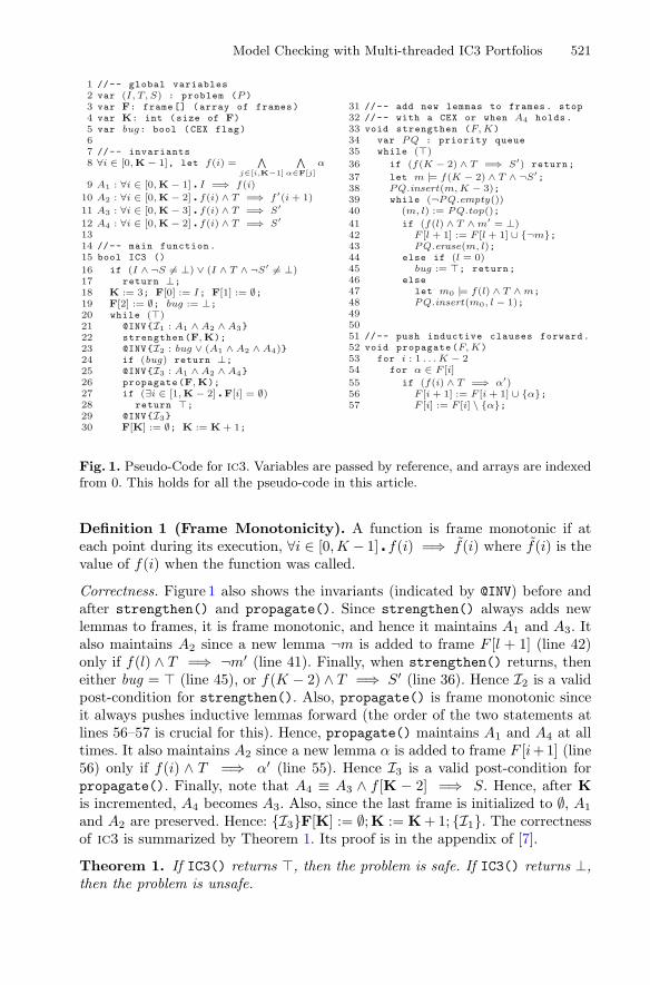
We begin with a description of the sequential ic3 algorithm. Figure 1 shows itspseudo-code. ic3 works as follows: (i) checks that no state in ¬S is reachable in 0or 1 steps from some state in I (lines 16–17); (ii) iteratively construct an array offrames, each consisting of a set of clauses, as follows: (a) initialize the frame arrayand flags (lines 18–19); (b) strengthen() the frames by adding new clauses (line22); if a counterexample is found in this step (indicated by bug being set), ic3terminates (line 24); (c) otherwise, propagate() clauses that are inductive tothe next frame (line 26); if a proof of safety is found (indicated by an emptyframe), ic3 again terminates (lines 27–28); (d) add a new empty frame to theend of the array (line 30) and repeat from step (b). In the rest of this paper weuse the term “function” to mean a “procedure”, as opposed to a mathematicalfunction. In particular, we use terms “pdf” and “cdf” to mean probability andcumulative distribution functions of random variables, respectively.

Model Checking with Multi-threaded IC3 Portfolios 521

1 //-- global variables2 var (I, T, S) : problem (P )3 var F: frame [] (array of frames)4 var K: int (size of F)5 var bug: bool (CEX flag)67 //-- invariants8 ∀i ∈ [0,K − 1], let f(i) =

∧

j∈[i,K−1]

∧

α∈F[j]α

9 A1 : ∀i ∈ [0,K − 1] � I =⇒ f(i)

10 A2 : ∀i ∈ [0,K − 2] � f(i) ∧ T =⇒ f ′(i + 1)

11 A3 : ∀i ∈ [0,K − 3] � f(i) ∧ T =⇒ S′

12 A4 : ∀i ∈ [0,K − 2] � f(i) ∧ T =⇒ S′

1314 //-- main function.15 bool IC3 ()

16 if (I ∧ ¬S = ⊥) ∨ (I ∧ T ∧ ¬S′ = ⊥)17 return ⊥;18 K := 3; F[0] := I; F[1] := ∅;19 F[2] := ∅; bug := ⊥;20 while (�)21 @INV{I1 : A1 ∧ A2 ∧ A3}22 strengthen(F,K);23 @INV{I2 : bug ∨ (A1 ∧ A2 ∧ A4)}24 if (bug) return ⊥;25 @INV{I3 : A1 ∧ A2 ∧ A4}26 propagate(F,K);27 if (∃i ∈ [1,K − 2] � F[i] = ∅)28 return �;29 @INV{I3}30 F[K] := ∅; K := K + 1;

31 //-- add new lemmas to frames. stop32 //-- with a CEX or when A4 holds.33 void strengthen (F, K)34 var PQ : priority queue35 while (�)

36 if (f(K − 2) ∧ T =⇒ S′) return;

37 let m |= f(K − 2) ∧ T ∧ ¬S′;38 PQ.insert(m, K − 3);39 while (¬PQ.empty())40 (m, l) := PQ.top();41 if (f(l) ∧ T ∧ m′ = ⊥)42 F [l + 1] := F [l + 1] ∪ {¬m};43 PQ.erase(m, l);44 else if (l = 0)45 bug := �; return;46 else47 let m0 |= f(l) ∧ T ∧ m;48 PQ.insert(m0, l − 1);495051 //-- push inductive clauses forward.52 void propagate(F, K)53 for i : 1 . . . K − 254 for α ∈ F [i]

55 if (f(i) ∧ T =⇒ α′)56 F [i + 1] := F [i + 1] ∪ {α};57 F [i] := F [i] \ {α};

Fig. 1. Pseudo-Code for ic3. Variables are passed by reference, and arrays are indexedfrom 0. This holds for all the pseudo-code in this article.

Definition 1 (Frame Monotonicity). A function is frame monotonic if ateach point during its execution, ∀i ∈ [0,K − 1] � f(i) =⇒ f(i) where f(i) is thevalue of f(i) when the function was called.

Correctness. Figure 1 also shows the invariants (indicated by @INV) before andafter strengthen() and propagate(). Since strengthen() always adds newlemmas to frames, it is frame monotonic, and hence it maintains A1 and A3. Italso maintains A2 since a new lemma ¬m is added to frame F [l + 1] (line 42)only if f(l) ∧ T =⇒ ¬m′ (line 41). Finally, when strengthen() returns, theneither bug = (line 45), or f(K − 2) ∧ T =⇒ S′ (line 36). Hence I2 is a validpost-condition for strengthen(). Also, propagate() is frame monotonic sinceit always pushes inductive lemmas forward (the order of the two statements atlines 56–57 is crucial for this). Hence, propagate() maintains A1 and A4 at alltimes. It also maintains A2 since a new lemma α is added to frame F [i+1] (line56) only if f(i) ∧ T =⇒ α′ (line 55). Hence I3 is a valid post-condition forpropagate(). Finally, note that A4 ≡ A3 ∧ f [K − 2] =⇒ S. Hence, after Kis incremented, A4 becomes A3. Also, since the last frame is initialized to ∅, A1

and A2 are preserved. Hence: {I3}F[K] := ∅;K := K+ 1; {I1}. The correctnessof ic3 is summarized by Theorem 1. Its proof is in the appendix of [7].

Theorem 1. If IC3() returns , then the problem is safe. If IC3() returns ⊥,then the problem is unsafe.

522 S. Chaki and D. Karimi

58 //-- global variables59 var (I, T, S) : problem (P )60 var ∀i ∈ [1, n] � Fi: frame []61 var K: int (size of each Fi)62 var bug: bool (CEX flag)6364 //-- invariants65 ∀j ∈ [0,K − 1], let66 f(j) =

∧

i∈[1,n]

∧

k∈[j,K−1]

∧

α∈Fi[k]α

6768 B1 : ∀j ∈ [0,K − 1] � I =⇒ f(j)

69 B2 : ∀j ∈ [0,K − 2] � f(j) ∧ T =⇒ f ′(j + 1)

70 B3 : ∀j ∈ [0,K − 3] � f(j) ∧ T =⇒ S′

71 B4 : ∀j ∈ [0,K − 2] � f(j) ∧ T =⇒ S′

72 bool IC3Sync (n)

73 if (I ∧ ¬S = ⊥) ∨ (I ∧ T ∧ ¬S′ = ⊥)74 return ⊥;75 K := 3; bug := ⊥;76 ∀i ∈ [1, n] � Fi[0] := I; Fi[1] := Fi[2] := ∅;77 while (�)78 @INV{I4 : B1 ∧ B2 ∧ B3}79 {strengthen(F1,K); propagate(F1,K)}80 ‖ · · · ‖81 {strengthen(Fn,K); propagate(Fn,K)};82 @INV{I5 : bug ∨ (B1 ∧ B2 ∧ B4)}83 if (bug) return ⊥;84 @INV{I6 : B1 ∧ B2 ∧ B4}85 if (∃j ∈ [1,K − 2] � ∀i ∈ [1, n] � Fi[j] = ∅)86 return �;87 @INV{I6}88 ∀i ∈ [1, n] � Fi[K] := ∅; K := K + 1;

Fig. 2. Pseudo-Code for ic3sync(n). Functions strengthen() and propagate() aredefined in Fig. 1.

We now present the three versions of parallel ic3 and their correctness (theirtermination follows in the same way as ic3 [6] – see Theorem 5 in the appendixof [7]).

4.1 Synchronous Parallel IC3

The first parallelized version of ic3, denoted ic3sync, runs a number of copies ofthe sequential ic3 “synchronously” in parallel. Let ic3sync(n) be the instanceof ic3sync consisting of n copies of ic3 executing concurrently. The copiesmaintain separate frames. However, for any copy, the frames of other copiesact as “background lemmas”. Specifically, the copies interact by: (i) using theframes of all other copies when computing f(i); (ii) declaring the problem unsafeif any copy finds a counterexample; (iii) declaring the problem safe if some framebecomes empty across all the copies; and (iv) “synchronizing” after each call tostrengthen() and propagate().

The pseudo-code for ic3sync(n) is shown in Fig. 2. The main function isIC3Sync(). After checking the base cases (lines 73–74), it initializes flags andframes (lines 75–76), and then iteratively performs the following steps: (i) runn copies ic3 where each copy does a single step of strengthen() followed bypropagate() (lines 79–81); (ii) check if any copy of ic3 found a counterexample,and if so, terminate (line 83); (iii) check if a proof of safety has been found, and ifso, terminate (lines 85–86); and (iv) add a frame and repeat from step (i) above(line 88). Functions strengthen() and propagate() are syntactically identicalto ic3 (cf. Fig. 1). However, the key semantic difference is that lemmas from allcopies are used to define f(j) (lines 65–66). Global variables are shared, andaccessed atomically. Note that even though all ic3 copies write to variable bug ,there is no race condition since they always write the same value ( ).

Correctness. The correctness of ic3sync follows from the invariants specified inFig. 2. To show these invariants are valid, the main challenge is to show thatif I4 holds at line 78, then I5 holds at line 82. Note that since strengthen()

Model Checking with Multi-threaded IC3 Portfolios 523

and propagate() are frame monotonic, they preserve B1 and B3. This meansthat B1 ∧ B3 holds at line 82. Now suppose that at line 82, we have ¬bug . Thismeans that each strengthen() called at lines 79–81 returned from line 36. Thus,the condition f(K − 2) ∧ T =⇒ S′ was established at some point, and onceestablished, it continues to hold due to the frame monotonicity of strengthen()and propagate(). Since B4 ≡ B3 ∧ (f(K − 2) ∧ T =⇒ S′), we therefore knowthat B1 ∧ B4 holds at line 82. Also, B2 holds at line 82 since a new lemma α isonly added to frame Fi[j +1] by strengthen() (line 42) and propagate() (line56) under the condition f(j)∧T =⇒ α′. Note that once f(j)∧T =⇒ α′ is true,it continues to hold even in the concurrent setting due to frame monotonicity.Finally, the statement at line 88 transforms I6 to I4. The correctness of ic3syncis summarized by Theorem 2. Its proof is in the appendix of [7].

Theorem 2. If IC3Sync() returns , then the problem is safe. If IC3Sync()returns ⊥, then the problem is unsafe.

89 //-- invariants90 ∀j ∈ [0,max(K1, . . . ,Kn) − 1], let91 f(j) =

∧

i∈[1,n]

∧

k∈[j,Ki−1]

∧

α∈Fi[k]α

9293 C1 : ∀j ∈ [0,Ki − 1] � I =⇒ f(j)

94 C2 : ∀j ∈ [0,Ki − 2] � f(j) ∧ T =⇒ f ′(j + 1)

95 C3 : ∀j ∈ [0,Ki − 3] � f(j) ∧ T =⇒ S′

96 C4 : ∀j ∈ [0,Ki − 2] � f(j) ∧ T =⇒ S′

979899

100 //-- top -level function101 bool IC3Async (n)

102 if (I ∧ ¬S = ⊥) ∨ (I ∧ T ∧ ¬S′ = ⊥)103 return ⊥;104 bug := ⊥;105 IC3Copy(1) � · · · � IC3Copy(n);106 return bug ? ⊥ : �;

107 //-- global variables108 var (I, T, S) : problem (P )109 var ∀i ∈ [1, n] � Fi: frame []110 var ∀i ∈ [1, n] � Ki: int (size of Fi)111 var bug: bool (CEX flag)112113 void IC3Copy (i)114 Ki := 3; Fi[0] := I;115 Fi[1] := ∅; Fi[2] := ∅;116 while (�)117 @INV{I7 : C1 ∧ C2 ∧ C3}118 strengthen(Fi,Ki);119 @INV{I8 : bug ∨ (C1 ∧ C2 ∧ C4)}120 if (bug) return;121 @INV{I9 : C1 ∧ C2 ∧ C4}122 propagate(Fi,Ki);123 if (∃j ∈ [1,Ki − 2] � ∀l ∈ [1, n] � Fl[j] = ∅)124 return;125 @INV{I9}126 Fi[Ki] := ∅; Ki := Ki + 1;

Fig. 3. Pseudo-Code for ic3async(n). Functions strengthen() and propagate() aredefined in Fig. 1.

4.2 Asynchronous Parallel IC3

The next parallelized version of ic3, denoted ic3async, runs a number of copiesof the sequential ic3 “asynchronously” in parallel. Let ic3async(n) be theinstance of ic3async consisting of n copies of ic3 executing concurrently. Sim-ilar to ic3sync, the copies maintain separate frames, interact by sharing lem-mas when computing f(i), and declare the problem unsafe if any copy finds acounterexample. However, due to the lack of synchronization, proof detection isdistributed over all the copies instead of being centralized in the main thread.

Figure 3 shows the pseudo-code for ic3async(n). The main function isIC3Async(). After checking the base cases (lines 102–103), it initializes flags

524 S. Chaki and D. Karimi

(line 104), launches n copies of ic3 in parallel (line 105) and waits for some copyto terminate (the � operator), and checks the flag and returns with an appropri-ate result (line 106). Function IC3Copy() is similar to IC3() in Fig. 1. The keydifference is that lemmas from all copies are used to compute f(j) (lines 90–91).

Correctness. The correctness of ic3async follows from the invariants specifiedin Fig. 3. To see why these invariants are valid, note that C1 and C3 are alwayspreserved due to frame monotonicity. If strengthen() returns with bug = ⊥,then it returned from line 36, and hence f(Ki −2)∧T =⇒ S′ was true at somepoint in the past and continues to hold due to frame monotonicity. Togetherwith C3, this implies that C4 holds at line 119. Also, C2 holds at line 119 sincea new lemma α is only added to frame Fi[j + 1] by strengthen() (line 42) andpropagate() (line 56) under the condition f(j) ∧ T =⇒ α′. Note that oncef(j) ∧ T =⇒ α′ is true, it continues to hold even under concurrency due toframe monotonicity. Hence, I8 holds at line 119. Since bug is never set to ⊥ afterline 104, this means that I9 holds at line 121 even under concurrency. Finally,the statement at line 126 transforms I9 to I7. The correctness of ic3async issummarized by Theorem 3. Its proof is in the appendix of [7].

Theorem 3. If IC3Async() returns , then the problem is safe. If IC3Async()returns ⊥, then the problem is unsafe.

127 //-- global variables128 var (I, T, S) : problem (P )129 var ∀i ∈ [1, n] � Fi,Pi: frame []130 var ∀i ∈ [1, n] � Ki: int (size of Fi and Pi)131 var bug, safe: bool (CEX and proof flags)132133134 void IC3PrCopy (i)135 Ki := 3; Fi[0] := I;136 Fi[1] := ∅; Fi[2] := ∅;137 while (�)138 @INV{I7 : C1 ∧ C2 ∧ C3}139 strengthen(Fi,Ki);140 @INV{I8 : bug ∨ (C1 ∧ C2 ∧ C4)}141 if (bug) return;142 @INV{I9 : C1 ∧ C2 ∧ C4}143 propProof(Fi,Ki);144 if (safe) return;145 @INV{I9}146 Fi[Ki] := ∅; Ki := Ki + 1;

147 bool IC3Proof (n)

148 if (I ∧ ¬S = ⊥) ∨ (I ∧ T ∧ ¬S′ = ⊥)149 return ⊥;150 bug := ⊥; safe := ⊥;151 IC3PrCopy(1) � · · · � IC3PrCopy(n);152 return bug ? ⊥ : �;153154 void propProof(F, K)155 for j : 1 . . . K − 2156 for α ∈ F [j]

157 if (f(j) ∧ T =⇒ α′)158 F [j + 1] := F [j + 1] ∪ {α};159 F [j] := F [j] \ {α};160 if (F [j] = ∅)161 Pj :=

⋃

j<k≤K−1F [k];

162 Π :=⋃

{i|1≤i≤n∧j<Ki}Pi;

163 if (Π ∧ T =⇒ Π′)164 safe := �; return;

Fig. 4. Pseudo-Code for ic3proof(n). Function strengthen() is defined in Fig. 1.Formulas f(j), I7, I8, and I9 are defined in Fig. 3.

4.3 Asynchronous Parallel IC3 with Proof-Checking

The final parallelized version of ic3, denoted ic3proof, is similar to ic3async,but performs more aggressive checking for proofs. Let ic3proof(n) be theinstance of ic3proof consisting of n copies of ic3 executing concurrently. Simi-lar to ic3async, the copies maintain separate frames, interact by sharing lemmas

Model Checking with Multi-threaded IC3 Portfolios 525

when computing f(i), and declare the problem unsafe if any copy finds a coun-terexample. However, whenever a copy finds an empty frame, it checks whetherthe set of lemmas over all the copies for that frame forms an inductive invariant.

The pseudo-code for ic3proof(n) is shown in Fig. 4. The main function isIC3Proof(). After checking the base cases (lines 148–149), it initializes flags(line 150), launches n copies of ic3 in parallel (line 151) and waits for at leastone copy to terminate, and checks the flag and returns with an appropriate result(line 152). Function IC3PrCopy is similar to IC3 in Fig. 1, but calls propProof()instead of propagate() where, once an empty frame is detected (line 160), wecheck whether a proof has been found by collecting the lemmas for that frame(lines 161–162), and checking if these lemmas are inductive (line 163).

Correctness. The correctness of ic3proof follows from the invariants (whosevalidity is similar to those for ic3async) specified in Fig. 4. It is summarized byTheorem 4. The proof of the theorem is in the appendix of [7].

Theorem 4. If IC3Proof() returns , then the problem is safe. If IC3Proof()returns ⊥, then the problem is unsafe.

5 Parallel ic3 Portfolios

In this section, we investigate the question of how a good portfolio size canbe selected if we want to implement a portfolio of ic3pars. We begin with anargument about the pdf of the runtime of ic3async(n).

Conjecture 1. The runtime of ic3async(n) converges to a Weibull rv as n → ∞.

Argument: Recall that each execution of ic3async(n) consists of n copies ofic3 running in parallel, and that ic3async(n) stops as soon as one copy finds asolution. We can consider the runtime of each copy of ic3 to be a rv. Specifically,let rv Xi be the runtime of the i-th copy of ic3 under the environment providedby the other n − 1 copies. Recall that the pdf of Xi has a lower bound of 0,since no run of ic3 can take negative time. Also, for the sake of argument,assume that (X1, . . . , Xn) are i.i.d. since the interaction between the copies ofic3 is logical and symmetric. Finally, let X be the random variable denoting theruntime of ic3async(n). Note that X = min(X1, . . . , Xn). Hence, by the EVT,X ∼ wei(k, λ) for large n. ��

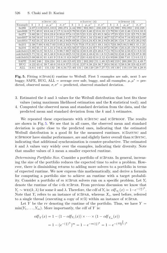
A similar argument holds for ic3sync and ic3proof, and therefore their run-time should follow Weibull as well. Indeed, despite the assumption of (X1, . . . , Xn)being i.i.d., we empirically find that the runtime of ic3par(n) follows a Weibulldistribution closely for even modest values of n. Specifically, we selected 10examples (5 safe and 5 buggy) from HWMCC14, and for each example we:

1. Executed ic3async(4) “around” 3000 times (we actually ran each example3000 times but some timed out – the exact number of timeouts varied acrossexamples);

2. Measured the runtimes;

526 S. Chaki and D. Karimi

ic3sync (4) ic3async (4) ic3proof (4)Example k λ μ, μ∗ σ, σ∗ k λ μ, μ∗ σ, σ∗ k λ μ, μ∗ σ, σ∗

6s286 4.07 1119 1015,1015 280,274 4.44 990 902,903 230,220 4.35 980 892,892 232,228intel026 2.71 49.0 43.6,44.2 17.3,14.6 3.70 50.2 45.3,46.2 13.6,10.1 3.70 50.1 45.2,46.1 13.6,10.36s273 3.80 26.1 23.6,23.6 6.93,6.57 4.11 23.5 21.3,21.4 5.85,5.36 4.17 23.3 21.2,21.3 5.73,5.29

intel057 6.58 16.0 14.9,15.1 2.66,2.11 7.31 17.2 16.1,16.1 2.60,2.46 7.52 17.8 16.7,16.9 2.63,2.07intel054 7.82 24.3 22.8,23.0 3.46,2.94 8.69 26.1 24.6,24.8 3.38,2.84 9.26 26.1 24.7,24.8 3.20,2.92

6s215 2.38 7.69 6.82,7.03 3.05,2.34 4.71 6.75 6.17,6.21 1.49,1.34 4.72 6.38 5.84,5.90 1.41,1.216s216 1.95 35.1 31.1,31.0 16.6,16.9 3.56 27.5 24.8,24.9 7.74,6.97 2.78 28.1 25.0,25.1 9.74,9.05

oski3ub1i 5.98 54.9 50.9,51.4 9.90,7.90 7.02 52.3 48.9,49.2 8.20,6.71 4.78 54.8 50.2,50.8 11.9,9.53oski3ub3i 5.71 52.4 48.5,48.9 9.84,8.00 5.51 52.2 48.2,48.6 10.1,8.51 5.66 52.2 48.2,48.5 9.87,8.39oski3ub5i 5.08 66.8 61.4,61.9 13.8,11.6 4.94 67.2 61.6,62.0 14.2,12.4 4.93 66.2 60.7,61.1 14.0,12.1

SAFE 5.00 246 224,224 62.1,60.2 5.65 221 202,202 51.1,48.3 5.80 219 200,200 51.4,49.7BUG 4.22 43.4 39.7,40.0 10.6,9.37 5.15 41.2 37.9,38.2 8.36,7.20 4.58 41.5 38.0,38.3 9.42,8.07ALL 4.61 145 131,132 36.4,34.7 5.40 131 120,120 29.7,27.7 5.19 130 119,119 30.4,28.9

Fig. 5. Fitting ic3par(4) runtime to Weibull. First 5 examples are safe, next 5 arebuggy; SAFE, BUG, ALL = average over safe, buggy, and all examples; μ, μ∗ = pre-dicted, observed mean; σ, σ∗ = predicted, observed standard deviation.

3. Estimated the k and λ values for the Weibull distribution that best fits thesevalues (using maximum likelihood estimation and the R statistical tool); and

4. Computed the observed mean and standard deviation from the data, and thepredicted mean and standard deviation from the k and λ estimates.

We repeated these experiments with ic3sync and ic3proof. The resultsare shown in Fig. 5. We see that in all cases, the observed mean and standarddeviation is quite close to the predicted ones, indicating that the estimatedWeibull distribution is a good fit for the measured runtimes. ic3async andic3proof have similar performance, are and slightly faster overall than ic3sync,indicating that additional synchronization is counter-productive. The estimatedk and λ values vary widely over the examples, indicating their diversity. Notethat smaller values of λ mean a smaller expected runtime.

Determining Portfolio Size. Consider a portfolio of ic3pars. In general, increas-ing the size of the portfolio reduces the expected time to solve a problem. How-ever, there is diminishing returns to adding more solvers to a portfolio in termsof expected runtime. We now express this mathematically, and derive a formulafor computing a portfolio size to achieve an runtime with a target probabil-ity. Consider a portfolio of m ic3par solvers run on a specific problem. Let Yi

denote the runtime of the i-th ic3par. From previous discussion we know thatYi ∼ wei(k, λ) for some k and λ. Therefore, the cdf of Yi is: cdf Yi

(x) = 1−e−( xλ )k

.Note that Yi refers to an instance of ic3par, whereas Xi, used before, referredto a single thread (executing a copy of ic3) within an instance of ic3par.

Let Y be the rv denoting the runtime of the portfolio. Thus, we have Y =min(Y1, . . . , Ym). More importantly, the cdf of Y is:

cdf Y (x) = 1 − (1 − cdfY1(x)) × · · · × (1 − cdf Ym(x))

= 1 − (e−( xλ )k

)m = 1 − e−m( xλ )k

= 1 − e−( xm1k

λ )k

Model Checking with Multi-threaded IC3 Portfolios 527

Note that this means Y is also a Weibull rv, not just when m → ∞ (asper the EVT) but for all m. More specifically, Y ∼ wei(k, λ

m1k

). Recall that ifm = 1, then the expected time to solve the problem by the portfolio is E[Y1].We refer to this time as t∗, the expected solving time for a single ic3par. Recallthe Gamma function Γ . Since Y1 ∼ wei(k, λ), it is known that t∗ = λΓ (1 + 1

k ).Now, we come to our result, which expresses the probability that a portfolio ofm ic3pars will require no more than t∗ to solve the problem.

Theorem 5. Let p(m) be the probability that Y ≤ t∗. Then p(m) > 1 − e− meγ

where γ ≈ 0.57721 is the Euler-Mascheroni constant.

Proof. We know that:

p(m) = cdf Y (t∗) = 1 − e−m(Γ (1+ 1k ))k

= 1 − (α(k))m, where α(k) = e−(Γ (1+ 1k ))k

Next, observe that α(k) increases monotonically with k but does not diverge ask → ∞. For example, Fig. 11 in the appendix of [7] shows a plot of α(k). Since wewant to prove an lower bound on p(m), let us consider the limiting case k → ∞.It can be shown that (see Lemma 2 in the appendix of [7]): limk→∞ α(k) = e− 1

eγ .In practice, as seen in Fig. 11 in the appendix of [7], the value of α(k) convergesquite rapidly to this limit as k increases. For example, α(5) > 0.91 · e− 1

eγ , andα(10) > 0.95 · e− 1

eγ . Since ∀k � α(k) < e− 1eγ , we have our result:

p(m) > 1−(e− 1eγ )m = 1−e− m

eγ ��

Achieving a Target Probability. Now suppose we want p(m) to be greater thansome target probability p. Then, from Theorem 5, we have:

p = 1 − (e− 1eγ )m ⇐⇒ 1 − p = e− m

eγ ⇐⇒ ln(1 − p) = − meγ

⇐⇒ ln( 11−p ) = m

eγ ⇐⇒ m = eγ ln( 11−p )

For example, if we want p = 0.99999, then m ≈ 20. Thus, a portfolio of 20ic3pars has about 0.99999 probability of solving a problem at least as quickly asthe expected time in which a single ic3par will solve it. We validated the efficacyof Theorem 5 by comparing its predictions with empirically observed resultson the HWMCC14 benchmarks. Overall, we find the observed and predictedprobabilities to agree significantly. Further details are presented in Sect. 6.3.

Speeding Up the Portfolio. To reduce the portfolio’s runtime below t∗, we mustincrease m appropriately. In general, for any constant c ∈ [0, 1], the probabilitythat a portfolio of m ic3par solvers will have a runtime ≤ c · t∗ is given by:

p(m, c, k) = 1 − e−m(c·Γ (1+ 1k ))k

For c < 1 we do not have a closed form for limk→∞

p(m, c, k), unlike when c = 1.

However, the value of p(m, c, k) is computable for fixed m, c and k. Figure 6(a)plots p(m, c, 4) for m = {1, . . . , 100} and c = {0.4, 0.5, 0.6}. Figure 6(b) plots

528 S. Chaki and D. Karimi

)b()a(

Fig. 6. (a) p(m, c, 4) for different values of c; (b) p(m, .5, k) for different values of k.

p(m, .5, k) for m = {1, . . . , 100} and k = {3, 4, 5}. As expected, p(m, c, k) increaseswith: (i) increasing m; (ii) increasing c; and (iii) decreasing k. One challenge hereis that we do not know how to estimate k for a problem without actually solvingit. In general, a smaller value of k means that a smaller portfolio will reach thetarget probability. In our experiments – recall Fig. 5 – we observed k-values in atight range (1–10) for problems from HWMCC14. These numbers can serve asguidelines, and be refined based on additional experimentation.

6 Experimental Results

We implemented ic3sync, ic3async and ic3proof by modifying a publiclyavailable reference implementation of ic3 (https://github.com/arbrad/IC3ref),which we call ic3ref. All propositional queries in ic3 are implemented by callsto minisat. We refer to the variant of ic3ref that uses a randomized minisat

as ic3rnd. We use ic3rnd to introduce uncertainty in ic3 purely by random-izing the backend SAT solver. We performed two experiments – one to evaluatethe effectiveness of the ic3par variants, and another to validate our statisticalanalysis of their portfolios. All our tools and results are available at http://www.andrew.cmu.edu/∼schaki/misc/paric3.tgz.

Benchmarks. We constructed four benchmarks. The first was constructed by pre-processing the safe examples from HWMCC14 (http://fmv.jku.at/hwmcc14cav)with iimc (http://ecee.colorado.edu/wpmu/iimc), and selecting the ones solvedby ic3ref within 900 s on a 8 core 3.4 GHz machine with 8GB of RAM. Theremaining three benchmarks were constructed similarly from the buggy examplesfrom HWMCC14, and the safe and buggy examples (without pre-processing)from the TIP benchmark suite (http://fmv.jku.at/aiger/tip-aig-20061215.zip).We refer to the four benchmarks as hwcsafe, hwcbug, tipsafe and tipbug,respectively.

Model Checking with Multi-threaded IC3 Portfolios 529

SAT Solver Pool. The function f (cf. Fig. 1–4) is implemented in ic3ref by aSAT solver (minisat). A separate SAT solver Si is used for each f(i). Wheneverf(i) changes due to the addition of a new lemma to a frame, the correspondingsolver Si is also updated by asserting the lemma. To avoid a single SAT solverfrom becoming the bottleneck between competing threads in ic3par, we use a“pool” of minisat solvers to implement each Si. The solvers are maintained in aFIFO queue. When a thread requests a solver, the first available solver is givento it. When a lemma is added to the pool, it is added to all available solvers,and recorded as “pending” for the busy ones. When a busy solver is released bya thread, all pending lemmas are first asserted to it, and then it is inserted atthe back of the queue. We refer to the number of solvers in each pool as SPSz.

6.1 Comparing Parallel ic3 Variants

These experiments were carried on a Intel Xeon machine with 128 cores, eachrunning at 2.67 GHz, and 1TB of RAM. For each solver selected from{ic3async(4), ic3sync(4), ic3proof(4), ic3rnd} and each benchmark B, andwith SPSz = 3, we performed the following steps:

1. extract all problems from B that are solved by ic3ref in at least 10 s; callthis set B∗; the cutoff of 10 s was a tradeoff between problem complexity andbenchmark size; our goal was to avoid evaluating our approach on very simpleexamples to limit measurement errors, and also to have enough examples forstatistically meaningful results;

2. solve each problem in B∗ with ic3ref and also with a portfolio of 20 solvers,compute the ratio of the two runtimes; this is the speedup for the specificproblem;

3. compute the mean and max of the speedups over all problems in B∗.

Figure 7(a) shows the results obtained. In all cases, we see speedup. Onthis particular run, ic3proof performs best overall, with an average speedupof over 6 and a maximum speedup of over 300. As in the non-portfolio case

ic3sync ic3async ic3proof ic3rnd

B |B∗| Mean Max Mean Max Mean Max Mean Maxhwcsafe 31 1.30 5.61 1.58 5.47 1.60 4.08 1.17 4.64hwcbug 14 2.49 18.7 14.3 151 25.1 309 1.07 1.49tipsafe 14 1.28 4.50 2.61 11.1 2.29 12.8 1.37 3.80tipbug 9 2.23 5.35 2.82 7.32 3.50 12.1 1.16 2.17

safe 44 1.30 5.61 1.93 11.1 1.83 12.8 1.24 4.64bug 23 2.38 18.7 9.58 151 16.3 309 1.11 2.17

all 67 1.67 18.7 4.74 151 6.79 309 1.19 4.64

ic3par2010

B |B+| Mean Maxhwcsafe 20 2.67 14.40hwcbug 15 1.62 3.91tipsafe 14 .89 1.82tipbug 7 1.32 1.67

safe 34 1.94 14.40bug 22 1.52 3.91

all 56 1.77 14.40

)b()a(

Fig. 7. (a) Speedup of ic3sync, ic3async, ic3proof and ic3rnd compared to ic3ref;(b) Speedup of ic3par2010 compared to ic3ref2010.

530 S. Chaki and D. Karimi

(cf. Fig. 5) ic3proof and ic3async have similar performance, and are bet-ter than ic3sync. The pattern is followed for both safe and buggy examples.Finally, ic3rnd provides mediocre speedup (not just on the whole, but acrossall examples) indicating that parallelization enables better search for shorterproofs/CEXes compared to randomizing the SAT solver.

ρ - ic3async ρ - ic3sync ρ - ic3proof

Example Mean StDev Mean StDev Mean StDev6s286 1.0000 0.0016 1.0010 0.0046 0.9996 0.0032

intel026 1.0042 0.0233 1.0028 0.0163 1.0027 0.01636s273 1.0025 0.0122 1.0031 0.0149 1.0030 0.0154

intel057 0.9968 0.0214 0.9855 0.0381 1.0002 0.0136intel054 1.0029 0.0162 0.9998 0.0076 0.9994 0.0080

6s215 1.0001 0.0057 0.9988 0.0099 0.9991 0.00586s216 1.0038 0.0204 1.0025 0.0163 1.0034 0.0182

oski3ub1i 1.0063 0.0321 1.0055 0.0293 1.0049 0.0274oski3ub3i 1.0042 0.0230 1.0049 0.0259 1.0053 0.0272oski3ub5i 1.0061 0.0312 1.0070 0.0358 1.0069 0.0357

0.5 0.6 0.7 0.8 0.9 1.00.

50.

60.

70.

80.

91.

0Predicted Probability

Obs

erve

d Pr

obab

ility

)b()a(

Fig. 8. Validating Theorem 5; (a) mean and standard deviation of ratios of predictedand observed probabilities; (b) scatter plot of predicted and observed probabilities.

6.2 Comparing ic3par2010

We compared the parallel version of ic3 reported in the original paper [6], whichwe refer to as ic3par2010, with our ic3par variants. We first downloaded thesource code1 of ic3par2010. It comes with its own version of ic3 implementedin Ocaml, which we refer to as ic3ref2010. The parallelization in ic3par2010

is implemented via three Python scripts that invoke the ic3 binary. We modifiedthese scripts to implement a solver with four copies of ic3 running in parallel.This was done for a fairer comparison with our ic3par results presented earlierwhich also used four copies of ic3 per solver. In addition, we made other changesto the scripts to make the solver more robust (e.g., replacing hard coded TCP/IPport numbers with dynamically selected ones). All experiments were done on thesame machine as in Sect. 6.1.

While ic3ref was quite deterministic in its runtime, ic3ref2010 demon-strated random behavior in this respect. One source of this randomness is thatic3ref2010 randomizes the backend SAT solver. However, there could be othersources of randomness due to the management of the priority queue duringstrengthen(). We were unable to eliminate the randomness satisfactorily viacommand line options. Instead, we accounted for it by running experiments mul-tiple times and computing the average. We computed the speedup of ic3par2010using a similar process as for the ic3par variants. Specifically, we performed thefollowing steps:1 http://ecee.colorado.edu/∼bradleya/ic3/ic3.tar.gz.

Model Checking with Multi-threaded IC3 Portfolios 531

1. extract all problems from B that are solved by ic3ref2010 in at least 10s;call this set B+; note that B+ differs from B∗ since the underlying solvers –ic3ref2010 and ic3ref – have different solving capability.

2. solve each problem in B+ with ic3ref2010 twenty times and compute theaverage runtime (call this ts) and also with ic3par2010 twenty times andcompute the average runtime (call this tp); compute the ratio ts

tp; this is the

speedup with ic3par2010 for that specific problem;3. compute the mean and max of the speedups over all problems in B+.

Figure 7(b) shows the results obtained. Comparing with Fig. 7(a), we seethat all three of our ic3par invariants provided considerably better speedupscompared to ic3par2010 on the three benchmark groups hwcbug, tipsafe

and tipbug. Indeed, for the tipsafe group as a whole, ic3par2010 does notprovide a speedup. However, for the hwcsafe group, ic3par2010 provided bet-ter speedups. If we look at all the safe examples, then ic3par2010 edges outic3par marginally. In contrast, for unsafe examples ic3par provides much betterspeedups. Overall, ic3proof performs best. In summary, portfolios of ic3par

variants appear to be a good complement to ic3par2010, and a better optionfor unsafe examples.

6.3 Portfolio Size

These experiments were done on a cluster of 11 machines, each with 16 cores at2.4 GHz, and between 48 GB and 190 GB of RAM. To validate Theorem 5, wecompared its predictions to empirically observed results as follows (again usingSPSz = 3):

1. Process each problem from Fig. 5 as follows.2. Solve the problem b (≈ 3000) times using ic3par(4). This gives a set of

runtimes t1, . . . , tb. Fit these runtimes to a Weibull distribution to obtain theestimated value of k (the same as the second column of Fig. 5).

3. Compute t = mean(t1, . . . , tb). This is the estimated average time for ic3par(4)to solve the problem.

4. Pick a portfolio size m. Start with m = 1.5. Divide t1, . . . , tb into blocks of size m. Let B = � b

m�. We now have B blocks ofruntime T1, . . . , TB , each consisting of m elements. Thus, T1 = {t1, . . . , tm},T2 = {tm+1, . . . , t2m}, and so on. For i = 1, . . . , B, compute μi = min(Ti).Note that each μi is the runtime of a portfolio of m ic3par(4) solvers.

6. Let n(m) be the number of blocks for which μi ≤ t, i.e., n(m) = |{i ∈ [1, B] | μi ≤ t}|. Compute p∗(m) = n(m)

B . Note that p∗(m) is the esti-mate of p(m) based on our experiments. Compute p(m) = 1 − (α(k))m (usek from Step 2). Compute ρ(m) = p∗(m)

p(m) . We expect ρ(m) ≈ 1.7. Repeat steps 5 and 6 with m = 2, . . . , 100 to obtain the sequence ρ =

〈ρ(1), . . . , ρ(100)〉. Compute the mean and standard deviation of ρ.

Figure 8(a) shows the results of the above steps for each ic3par variant.We see that for each example, the mean of ρ is very close to 1 and its standard

532 S. Chaki and D. Karimi

deviation is very close to 0, indicating that p(m) and p∗(m) agree considerably.Figure 8(b) shows a scatter plot of all p∗(m) values computed against their cor-responding p(m). Note that most values are very close to the (red) x = y line,as expected.

Fig. 9. Heatmap of ic3proof runtimes for three examples. Deeper color of cell (i, s)indicates that ic3proof(i, s) solves the benchmark faster; n = total number of runs ofic3proof over all 64 values of (i, s).

6.4 Parameter Sweeping

ic3par has two parameters: number of ic3 threads and SPSz. We write ic3par

(i, s) to mean an instance of ic3par with i ic3 threads and SPSz = s. Thus,ic3par(4, 3) was used is all previous experiments. We observed in Sect. 6.1 thatdifferent ic3par variants perform the best for different benchmarks. We nowevaluate the performance of ic3proof by varying i and s. These experimentswere also done on our cluster (cf. Sect. 6.3). We begin with a conjecture aboutthe relationship of runtime and parameter values.

Conjecture 2. The parameter value affects performance of ic3par significantly,and the best parameter choice is located unpredictably in the input space.

To investigate Conjecture 2, we measured the runtime of ic3proof(i, s) foreach (i, s) ∈ I × S where I = S = {1, . . . , 8}. We selected 16 examples fromB. For each example η, and each (i, s) ∈ I × S, we executed ic3proof(i, s) onη “around” 3000 times (again, the exact number varied across examples due totimeouts) and computed the average runtime. This gives us the entry at (i, s) forthe “heatmap” for η. The heatmaps in Fig. 9 summarize our results for three ofthe benchmarks that we found to be representative. They support Conjecture 2,as average runtimes (indicated by the color depth of cells in the heatmaps) acrossthe parameter space are varied. The depth of cells show no discernable pattern(e.g., do not increase with i or s), and the deepest cells are significantly moreso than the lightest ones. This implies that: (i) selecting the best parameters foric3proof would be quite beneficial; but (ii) this is a non-trivial problem.

As a preliminary step to address this challenge, we ran portfolios of a solverthat uses parameter sweeping [2]. Specifically, the solver (denoted ic3sweep)executes a randomly selected ic3par variant with a random (i, s) selected from

Model Checking with Multi-threaded IC3 Portfolios 533

Time SpeedupExample ic3ref Sync Async Proof Sweep6s286 947.6 1.54 1.57 1.66 1.77

intel026 78.33 2.61 2.77 2.85 2.586s273 31.06 1.84 1.88 1.90 1.65

intel057 31.33 2.45 2.49 2.49 2.66intel054 55.89 3.52 3.51 3.52 3.92Mean 2.39 2.44 2.48 2.52

Time SpeedupExample ic3ref Sync Async Proof Sweep6s215 12.20 2.47 2.57 2.61 2.366s216 67.24 4.33 4.35 4.30 4.29

oski3ub1i 83.64 1.90 1.97 1.94 1.96oski3ub3i 79.41 1.90 1.94 1.99 1.94oski3ub5i 127.3 2.66 2.65 2.67 2.76Mean 2.65 2.70 2.70 2.66

Fig. 10. Parameter sweeping; Sync, Async, Proof, Sweep = average speedups overic3ref for portfolios of 20 ic3sync (4,3), ic3async (4,3), ic3proof (4,3), andic3sweep, respectively.

I × S. We compared the average speedup (over 50 runs) of a portfolio of 20ic3sweeps with the average speedup (over 50 runs) of portfolios of 20 of eachof the three ic3par variants with fixed (i, s) = (4, 3). Figure 10 summarizes ourresults. We observe that in general ic3sweep is competitive with each of theic3par variants (indeed, it performs best for the hardest examples from the safeand buggy categories). We believe that parameter sweeping shows promise as astrategy for real-life problems where good parameters would be difficult (if notimpossible) to compute.

7 Conclusion

We present three ways to parallelize ic3. Each variant uses a number of threadsto speed up the computation of an inductive invariant or a CEX, sharing lemmasto minimize duplicated effort. They differ in the degree of synchronization andtechnique to detect if an inductive invariant has been found. The runtime ofthese solvers is unpredictable, and varies with thread-interleaving. We explorethe use of portfolios to counteract the runtime variance. Each solver in theportfolio potentially searches for a different proof/CEX. The first one to succeedprovides the solution. Using the Extreme Value theorem and statistical analysis,we construct a formula that gives us a portfolio size to solving a problem withina target time bound with a certain probability. Experiments on HWMCC14benchmarks show that the combination of parallelization and portfolios yieldsan average speedups of 6x over ic3, and in some cases speedups of over 300. Weshow that parameter sweeping is a promising approach to implement a solverthat performs well over a wide range of problems of unknown difficulty. Animportant area of future work is the effectiveness of parallelization and portfoliosin the context of software verification via a generalization of ic3 [12].

Aknowledgment. We are grateful to Jeffery Hansen and Arie Gurfinkel for helpfulcomments and discussions. This material is based upon work funded and supportedby the Department of Defense under Contract No. FA8721-05-C-0003 with CarnegieMellon University for the operation of the Software Engineering Institute, a federallyfunded research and development center. This material has been approved for publicrelease and unlimited distribution DM-0002752.

534 S. Chaki and D. Karimi

References

1. Albarghouthi, A., Kumar, R., Nori, A.V., Rajamani, S.K.: Parallelizing top-downinterprocedural analyses. In: Vitek, J., Lin, H., Tip, F. (eds.) Proceedings of theACM SIGPLAN 2012 Conference on Programming Language Design and Imple-mentation (PLDI 2012), pp. 217–228. Association for Computing Machinery, Bei-jing, China, June 2012

2. Ansel, J., Kamil, S., Veeramachaneni, K., Ragan-Kelley, J., Bosboom, J.,O’Reilly, U., Amarasinghe, S.P.: OpenTuner: an extensible framework for programautotuning. In: Amaral, J.N., Torrellas, J. (eds.) Proceedings of the 23rd Inter-national Conference on Parallel Architectures and Compilation (PACT 2014), pp.303–316. Association for Computing Machinery, Edmonton, AB, Canada, August2014

3. Barnat, J., et al.: DiVinE 3.0 - an explicit-state model checker for multithreadedC & C++ programs. In: Sharygina, N., Veith, H. (eds.) CAV. Lecture Notes inComputer Science, vol. 8044, pp. 863–868. Springer, Saint Petersburg (2013)

4. Bingham, B., Bingham, J., Erickson, J., de Paula, F.M., Reitblatt, M., Singh, G.:Industrial strength distributed explicit state model checking. In: Proceedings of the9th International Workshop on Parallel and Distributed Methods in verifiCation(PDMC 2010), Twente, The Netherlands, September-October 2010

5. Blom, S., van de Pol, J., Weber, M.: LTSmin: distributed and symbolic reachability.In: Touili, T., Cook, B., Jackson, P. (eds.) CAV 2010. LNCS, vol. 6174, pp. 354–359.Springer, Heidelberg (2010)

6. Bradley, A.R.: SAT-Based model checking without unrolling. In: Jhala, R.,Schmidt, D. (eds.) VMCAI 2011. LNCS, vol. 6538, pp. 70–87. Springer,Heidelberg (2011)

7. Chaki, S., Karimi, D.: Model Checking with Multi-Threaded IC3 Portfolios (2016),Extended version of this paper. http://www.contrib.andrew.cmu.edu/∼schaki/publications/VMCAI-2016-Extended.pdf

8. Cimatti, A., Griggio, A.: Software model checking via IC3. In: Madhusudan, P.,Seshia, S.A. (eds.) CAV 2012. LNCS, vol. 7358, pp. 277–293. Springer, Heidelberg(2012)

9. Ditter, A., Ceska, M., Luttgen, G.: On parallel software verification using booleanequation systems. In: Donaldson, A., Parker, D. (eds.) SPIN 2012. LNCS, vol.7385, pp. 80–97. Springer, Heidelberg (2012)

10. Een, N., Mishchenko, A., Brayton, R.K.: Efficient implementation of propertydirected reachability. In: Proceedings of the 11th International Conference on For-mal Methods in Computer-Aided Design (FMCAD 2011), pp. 125–134. IEEE Com-puter Society, Austin, TX, October-November 2011

11. de Haan, L., Ferreira, A.: Extreme Value Theory: An Introduction. Springer,New York (2006)

12. Hoder, K., Bjørner, N.: Generalized property directed reachability. In: Cimatti, A.,Sebastiani, R. (eds.) SAT 2012. LNCS, vol. 7317, pp. 157–171. Springer, Heidelberg(2012)

13. Holzmann, G.J.: Parallelizing the spin model checker. In: Donaldson, A., Parker,D. (eds.) SPIN 2012. LNCS, vol. 7385, pp. 155–171. Springer, Heidelberg (2012)

14. Kadioglu, S., Malitsky, Y., Sabharwal, A., Samulowitz, H., Sellmann, M.: Algo-rithm selection and scheduling. In: Lee, J. (ed.) CP 2011. LNCS, vol. 6876, pp.454–469. Springer, Heidelberg (2011)

Model Checking with Multi-threaded IC3 Portfolios 535

15. Lopes, N.P., Rybalchenko, A.: Distributed and predictable software model check-ing. In: Jhala, R., Schmidt, D. (eds.) VMCAI 2011. LNCS, vol. 6538, pp. 340–355.Springer, Heidelberg (2011)

16. Malitsky, Y., Sabharwal, A., Samulowitz, H., Sellmann, M.: Boosting sequen-tial solver portfolios: knowledge sharing and accuracy prediction. In: Nicosia, G.,Pardalos, P. (eds.) LION 7. LNCS, vol. 7997, pp. 153–167. Springer, Heidelberg(2013)

17. Melatti, I., Palmer, R., Sawaya, G., Yang, Y., Kirby, R.M., Gopalakrishnan, G.C.:Parallel and distributed model checking in eddy. In: Valmari, A. (ed.) SPIN 2006.LNCS, vol. 3925, pp. 108–125. Springer, Heidelberg (2006)

18. Palikareva, H., Cadar, C.: Multi-solver support in symbolic execution. In:Sharygina, N., Veith, H. (eds.) CAV 2013. LNCS, vol. 8044, pp. 53–68. Springer,Heidelberg (2013)

19. Ppfolio website. http://www.cril.univ-artois.fr/∼roussel/ppfolio20. Weibull, W.: A statistical distribution function of wide applicability. ASME J.

Appl. Mech. 18(3), 293–297 (1951)21. Wintersteiger, C.M., Hamadi, Y., de Moura, L.: A concurrent portfolio approach

to SMT solving. In: Bouajjani, A., Maler, O. (eds.) CAV 2009. LNCS, vol. 5643,pp. 715–720. Springer, Heidelberg (2009)

22. Xu, L., Hutter, F., Hoos, H.H., Leyton-Brown, K.: Satzilla: Portfolio-based algo-rithm selection for SAT. J. Artif. Intell. Res. (JAIR) 32, 565–606 (2008)