Model Checking Foundations and Applications Tevfik Bultan Department of Computer Science University...
124
Model Checking Foundations and Applications Tevfik Bultan Department of Computer Science University of California, Santa Barbara [email protected] http://www.cs.ucsb.edu/~bultan/
-
date post
19-Dec-2015 -
Category
Documents
-
view
216 -
download
0
Transcript of Model Checking Foundations and Applications Tevfik Bultan Department of Computer Science University...

Model Checking Foundations and Applications
Tevfik BultanDepartment of Computer Science
University of California, Santa [email protected]
http://www.cs.ucsb.edu/~bultan/

Outline
• Temporal Logics for Reactive Systems• Automated Verification of Temporal Properties of Finite
State Systems• Temporal Properties Fixpoints • Symbolic Model Checking
– SMV• LTL Properties Büchi automata
– SPIN• Infinite State Model Checking• Model Checking Programs
– SLAM project– Java Path Finder

Temporal Logics for Reactive Systems [Pnueli FOCS 77, TCS 81]
Transformational systems
get input;
compute something;
return result;
Reactive systems
while (true) {
receive some input,
send some output
}
• Transformational view follows from the initial use of computers as advanced calculators: A component receives some input, does some calculation and then returns a result.
• Nowadays, the reactive system view seems more natural: components which continuously interact with each other and their environment without terminating

Transformational vs. Reactive Systems
Transformational systems
get input;
{pre-condition}
compute something;
{post-condition}
return result;
Reactive systems
while (true) {
receive some input,
send some output
}
• Earlier work in verification uses the transformational view: – halting problem– Hoare logic– pre and post-conditions – partial vs. total correctness
• For reactive systems:– termination is not the main
issue– pre and post-conditions are
not enough

Reactive Systems: A Very Simple Model
• We will use a very simple model for reactive systems
• A reactive system generates a set of execution paths
• An execution path is a concatenation of the states (configurations) of the system, starting from some initial state
• There is a transition relation which specifies the next-state relation, i.e., given a state what are the states that can follow that state
• We need an example

A Mutual Exclusion Protocol
Process 1:while (true) { out: a := true; turn := true; wait: await (b = false or turn = false); cs: a := false;}||Process 2:while (true) { out: b := true; turn := false; wait: await (a = false or turn); cs: b := false;}
Two concurrently executing processes are trying to enter a critical section without violating mutual exclusion

State Space
• The state space of a program can be captured by the valuations of the variables and the program counters – you have to wait until the next lecture for a discussion
about the control stack (and recursion) and the heap (and dynamic memory allocation)
• For our example, we have– two program counters: pc1, pc2
domains of the program counters: {out, wait, cs}– three boolean variables: turn, a, b
boolean domain: {True, False}
• Each state of the program is a valuation of all the variables

State Space
• Each state can be written as a tuple (pc1,pc2,turn,a,b)
• Initial states: {(o,o,F,F,F), (o,o,F,F,T), (o,o,F,T,F), (o,o,F,T,T), (o,o,T,F,F), (o,o,T,F,T), (o,o,T,T,F), (o,o,T,T,T)}– initially: pc1=o and pc2=o
• How many states total?
3 * 3 * 2 * 2 * 2 = 72
exponential in the number of variables and the number of concurrent components

Transition Relation
• Transition Relation specifies the next-state relation, i.e., given a state what are the states that can come after that state
• For example, given the initial state (o,o,F,F,F)
Process 1 can execute:
out: a := true; turn := true;
or Process 2 can execute:
out: b := true; turn := false;• If process 1 executes, the next state is (w,o,T,T,F)• If process 2 executes, the next state is (o,w,F,F,T)• So the state pairs ((o,o,F,F,F),(w,o,T,T,F)) and ((o,o,F,F,F),(o,w,F,F,T)) are included in the transition relation

Transition Relation
The transition relation is like a graph, edges represent the next-state relation
(o,o,F,F,F)
(o,w,F,F,T) (w,o,T,T,F)
(o,c,F,F,T) (w,w,T,T,T)

Transition System
• A transition system T = (S, I, R) consists of– a set of states S– a set of initial states I S– and a transition relation R S S
• A common assumption in model checking– R is total, i.e., for all s S, there exists s’ such
that (s,s’) R

Execution Paths
• An execution path is an infinite sequence of states
x = s0, s1, s2, ...
such that
s0 I and for all i 0, (si,si+1) R
Notation: For any path x
xi denotes the i’th state on the path (i.e., si)
xi denotes the i’th suffix of the path (i.e., si, si+1, si+2, ... )

Execution Paths
A possible execution path:
((o,o,F,F,F), (o,w,F,F,T), (o,c,F,F,T))
( means repeat the above three states infinitely many times)
(o,o,F,F,F)
(o,w,F,F,T) (w,o,T,T,F)
(o,c,F,F,T) (w,w,T,T,T)
Temporal Logics
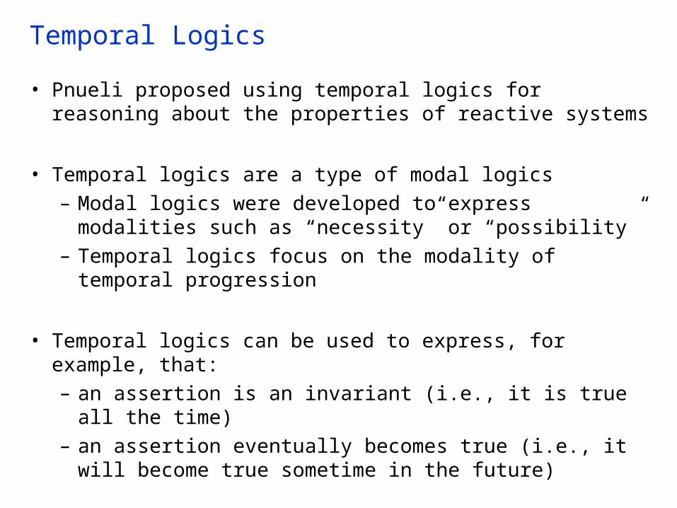
• Pnueli proposed using temporal logics for reasoning about the properties of reactive systems
• Temporal logics are a type of modal logics– Modal logics were developed to express modalities such
as “necessity” or “possibility”– Temporal logics focus on the modality of temporal
progression
• Temporal logics can be used to express, for example, that:– an assertion is an invariant (i.e., it is true all the time)– an assertion eventually becomes true (i.e., it will become
true sometime in the future)

Temporal Logics
• We will assume that there is a set of basic (atomic) properties called AP– These are used to write the basic (non-temporal)
assertions about the program– Examples: a=true, pc0=c, x=y+1
• We will use the usual boolean connectives: , ,
• We will also use four temporal operators:Invariant p : G p (aka p) (Globally)Eventually p : F p (aka p) (Future)Next p : X p (aka p) (neXt)p Until q : p U q

Atomic Properties
• In order to define the semantics we will need a function L which evaluates the truth of atomic properties on states:
L : S AP {True, False}
L((o,o,F,F,F), pc1=o) = True
L((o,o,F,F,F), pc1=w) = False
L((o,o,F,F,F), turn) = False
L((o,o,F,F,F), turn=false) = True
L((o,o,F,F,F), turn) = True
L((o,o,F,F,F), pc1=o pc2=o turn a b ) = True

Linear Time Temporal Logic (LTL) Semantics
Given an execution path x and LTL properties p and q
x |= p iff L(x0, p) =True, where p AP
x |= p iff not x |= p
x |= p q iff x |= p and x |= q
x |= p q iff x |= p or x |= q
x |= X p iff x1 |= p
x |= G p iff for all i, xi |= p
x |= F p iff there exists an i such that xi |= p
x |= p U q iff there exists an i such that xi |= q and
for all j < i, xj |= p

LTL Properties
p. . .
pp p p p p. . .
p. . .
pp p p q. . .
X p
G p
F p
p U q

Example Properties
mutual exclusion: G ( (pc1=c pc2=c))starvation freedom:
G(pc1=w F(pc1=c)) G(pc2=w F(pc2=c))
Given the execution path:x =((o,o,F,F,F), (o,w,F,F,T), (o,c,F,F,T))
x |= pc1=ox |= X (pc2=w)x |= F (pc2=c)x |= (turn) U (pc2=c b)x |= G ( (pc1=c pc2=c))x |= G(pc1=w F(pc1=c)) G(pc2=w F(pc2=c))

LTL Equivalences
• We do not really need all four temporal operators– X and U are enough (i.e., X, U, AP and boolean
connectives form a basis for LTL)
F p = true U p
G p = (Fp) = (true U p)

LTL Model Checking
• Given a transition system T and an LTL property p
T |= p iff for all execution paths x in T, x |= p
For example:
T |=? G ( (pc1=c pc2=c))
T |=? G(pc1=w F(pc1=c)) G(pc2=w F(pc2=c))
Model checking problem: Given a transition system T and an LTL property p, determine if T is a model for p (i.e., if T |=p)

Linear Time vs. Branching Time
• In linear time logics given we look at execution paths individually
• In branching time logics we view the computation as a tree– computation tree: unroll the transition relation
s2s1 s4s3
Transition System Execution Paths Computation Tree
s3
s4
s3
s3
s1
s2...
.
.
.
s3
s4
s3
s3
s1
s2
.
.
....
s3s4 s1...
.
.
....
s4 s1...

Computation Tree Logic (CTL)
• In CTL we quantify over the paths in the computation tree
• We use the same four temporal operators: X, G, F, U
• However we attach path quantifiers to these temporal operators:– A : for all paths– E : there exists a path
• We end up with eight temporal operators:– AX, EX, AG, EG, AF, EF, AU, EU

CTL Semantics
Given a state s and CTL properties p and q
s |= p iff L(s, p) =True, where p AP
s |= p iff not x |= p
s |= p q iff s |= p and s |= q
s |= p q iff s |= p or s |= q
s0 |= EX p iff there exists a path s0, s1, s2, ... such that s1
|= p
s0 |= AX p iff for all paths s0, s1, s2, ..., s1 |= p

CTL Semantics
s0 |= EG p iff there exists a path s0, s1, s2, ... such that
for all i, si |= p
s0 |= AG p iff for all paths s0, s1, s2, ..., for all i, si |= p
s0 |= EF p iff there exists a path s0, s1, s2, ... such that there exists an i such that si |= p
s0 |= AF p iff for all paths s0, s1, s2, ..., there exists an i, such that, si |= p
s0 |= p EU q iff there exists a path s0, s1, s2, ..., such that, there exists an i such that si |= q and for all j < i, sj
|= p
s0 |= p AU q iff for all paths s0, s1, s2, ..., there exists an i such that si |= q and for all j < i, sj
|= p

CTL Equivalences
• CTL basis: EX, EU, EG
AX p = EX p
AG p = EF p
AF p = EG p
p AU q = ( (q EU (p q)) EG q)
EF p = True EU p
• Another CTL basis: EX, EU, AU

CTL Properties
s2s1 s4s3
Transition System Computation Tree
s4
s3
s3
s1
s2
.
.
....
s3s4 s1...
.
.
....
s4 s1...
p pp
p
p
p
s3 |= ps4 |= ps1 |= ps2 |= p
s3 |= EX ps3 |= EX ps3 |= AX ps3 |= AX ps3 |= EG ps3 |= EG ps3 |= AF ps3 |= EF ps3 |= AF p
p
p

CTL Model Checking
• Given a transition system T= (S, I, R) and a CTL property p
T |= p iff for all initial state s I, s |= p
Model checking problem: Given a transition system T and a CTL property p, determine if T is a model for p (i.e., if T |=p)
For example:
T |=? AG ( (pc1=c pc2=c))
T |=? AG(pc1=w AF(pc1=c)) AG(pc2=w AF(pc2=c))
• Question: Are CTL and LTL equivalent?

CTL vs. LTL
• CTL and LTL are not equivalent– There are properties that can be expressed in LTL but
cannot be expressed in CTL • For example: FG p
– There are properties that can be expressed in CTL but cannot be expressed in LTL
• For example: AG(EF p)
• Hence, expressive power of CTL and LTL are not comparable
CTL*
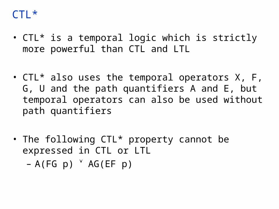
• CTL* is a temporal logic which is strictly more powerful than CTL and LTL
• CTL* also uses the temporal operators X, F, G, U and the path quantifiers A and E, but temporal operators can also be used without path quantifiers
• The following CTL* property cannot be expressed in CTL or LTL– A(FG p) AG(EF p)

Automated Verification of Finite State Systems [Clarke and Emerson 81], [Queille and Sifakis 82]
CTL Model checking problem: Given a transition system T = (S, I, R), and a CTL formula f, does the transition system satisfy the property?
CTL model checking problem can be solved in
O(|f| (|S|+|R|))
Note that the complexity is linear in the size of the transition system– Recall that the size of the transition system is
exponential in the number of variables and concurrent components (this is called the state space explosion problem)

CTL Model Checking Algorithm
• Translate the formula to a formula which uses the basis – EX p, EG p, p EU q
• Start from the innermost (non-atomic) subformulas and label the states in the transition system with the subformulas that hold in that state – Initially states are labeled with atomic properties
• Each (temporal or boolean) operator has to be processed once
• Computation of each subformula takes O(|S|+|R|)
CTL Model Checking Algorithm
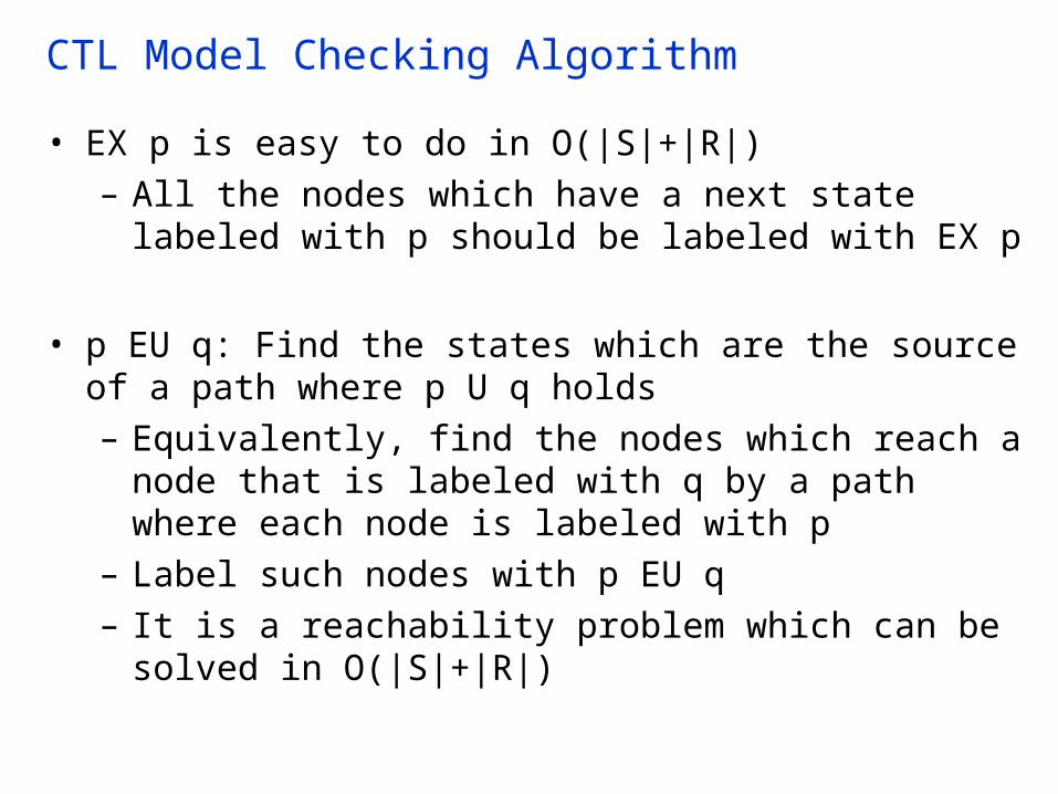
• EX p is easy to do in O(|S|+|R|)– All the nodes which have a next state labeled with p
should be labeled with EX p
• p EU q: Find the states which are the source of a path where p U q holds– Equivalently, find the nodes which reach a node that is
labeled with q by a path where each node is labeled with p
– Label such nodes with p EU q– It is a reachability problem which can be solved in O(|S|
+|R|)

CTL Model Checking Algorithm
• EG p: Find infinite paths where each node is labeled with p and label nodes in such paths with EG p– First remove all the states which do not satisfy p from
the transition graph– Compute the strongly connected components of the
remaining graph and then find the nodes which can reach the strongly connected components (both of which can be done in O(|S|+|R|)
– Label the nodes in the strongly connected components and that can reach the strongly connected components with EG p

Verification vs. Falsification
• Verification: – Show: initial states truth set of p
• Falsification:– Find: a state initial states truth set of p– Generate a counter-example starting from that state
• CTL model checking algorithm can also generate a counter-example path if the property is not satisfied– without increasing the complexity
• The ability to find counter-examples is one of the biggest strengths of the model checkers

What About LTL and CTL* Model Checking?
• The complexity of the model checking problem for LTL and CTL* are: – (|S|+|R|) 2O(|f|)
• Typically the size of the formula is much smaller than the size of the transition system – So the exponential complexity in the size of the formula
is not very significant in practice

Temporal Properties Fixpoints [Emerson and Clarke 80]
Here are some interesting CTL equivalences:
AG p = p AX AG pEG p = p EX EG p
AF p = p AX AF pEF p = p EX EF p
p AU q = q (p AX (p AU q))p EU q = q (p EX (p EU q))
Note that we wrote the CTL temporal operators in terms of themselves and EX and AX operators

Functionals
• Given a transition system T=(S, I, R), we will define functions from sets of states to sets of states – F : 2S 2S
• For example, one such function is the EX operator (which computes the precondition of a set of states)– EX : 2S 2S
which can be defined as:
EX(p) = { s | (s,s’) R and s’ p }
Abuse of notation: I am using p to denote the set of states which satisfy the property p

Functionals
• Now, we can think of all temporal operators also as functions from sets of states to sets of states
• For example:
AX p = EX(p)
or if we use the set notation
AX p = (S - EX(S - p))
Abuse of notation: I will use the set
and logic notations interchangeably.
Logic Setp q p qp q p q p S – pFalse True S

Lattice
The set of states of the transition system forms a lattice:
• lattice 2S
• partial order • bottom element • top element S• Least upper bound (aka join) operator• Greatest lower bound (aka meet) operator

Temporal Properties Fixpoints
Based on the equivalence EF p = p EX EF p we observe that EF p is a fixpoint of the following function: F y = p EX y F (EF p) = EF pIn fact, EF p is the least fixpoint of F, which is written as:
EF p = y . p EX y
Based on the equivalence EG p = p AX EG pwe observe that EG p is a fixpoint of the following function: F y = p EX y
F (EG p) = EG pIn fact, EG p is the greatest fixpoint of F, which is written as:
EG p = y . p EX y

Fixpoint Characterizations
Fixpoint Characterization Equivalences
AG p = y . p AX y AG p = p AX AG p
EG p = y . p EX y EG p = p EX EG p
AF p = y . p AX y AF p = p AX AF p
EF p = y . p EX y EF p = p EX EF p
p AU q = y . q (p AX (y)) p AU q=q (p AX (p AU q))
p EU q = y . q (p EX (y)) p EU q = q (p EX (p EU q))

Least and Greatest Fixpoints
The least and greatest fixpoint operators are defined as:
y . F y = { y | F y y } (glb of all the reductive elements)
y. F y = { y | F y y } (lub of all the extensive elements)
The least fixpoint y . F y is the limit of the following sequence (assuming F is -continuous):
, F , F2 , F3 , ...
The greatest fixpoint y . F y is the limit of the following sequence (assuming F is -continuous):
S, F S, F2 S, F3 S, ...
If S is finite, then we can compute the least and greatest fixpoints using these sequences
EF and EG computations
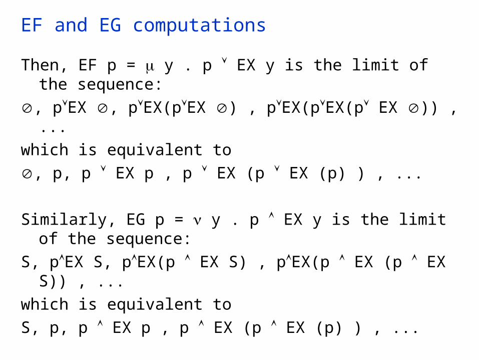
Then, EF p = y . p EX y is the limit of the sequence:
, pEX , pEX(pEX ) , pEX(pEX(p EX )) , ...
which is equivalent to
, p, p EX p , p EX (p EX (p) ) , ...
Similarly, EG p = y . p EX y is the limit of the sequence:
S, pEX S, pEX(p EX S) , pEX(p EX (p EX S)) , ...
which is equivalent to
S, p, p EX p , p EX (p EX (p) ) , ...

EF Fixpoint Computation
• • •• • •pp
EF(EF(pp)) states that can reach states that can reach p p p p EX( EX(pp)) EX(EX( EX(EX(pp)) )) ......
EF(EF(pp))

EG Fixpoint Computation
• • •• • • EG(EG(p)p)
EG(EG(pp)) states that can avoid reaching states that can avoid reaching pp p p EX( EX(pp)) EX(EX( EX(EX(pp)))) ......
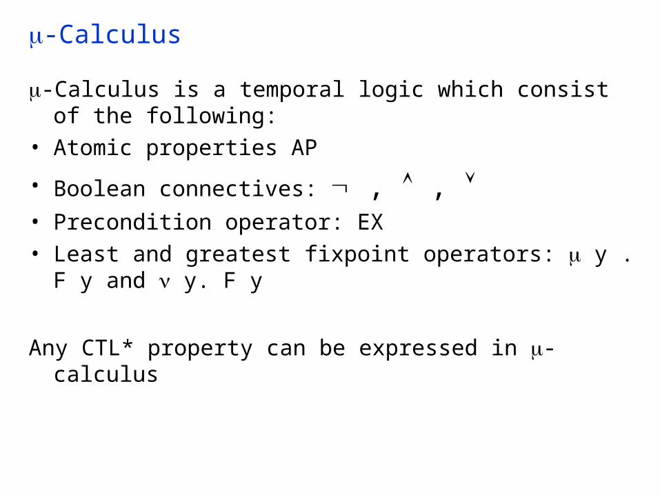
-Calculus
-Calculus is a temporal logic which consist of the following:• Atomic properties AP
• Boolean connectives: , , • Precondition operator: EX• Least and greatest fixpoint operators: y . F y and y. F y
Any CTL* property can be expressed in -calculus
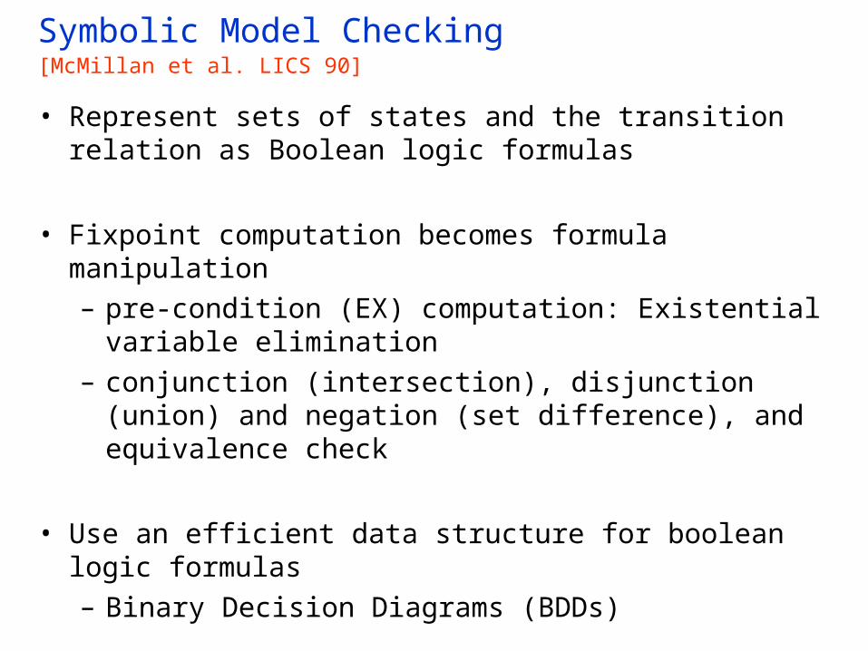
Symbolic Model Checking[McMillan et al. LICS 90]
• Represent sets of states and the transition relation as Boolean logic formulas
• Fixpoint computation becomes formula manipulation– pre-condition (EX) computation: Existential variable
elimination– conjunction (intersection), disjunction (union) and
negation (set difference), and equivalence check
• Use an efficient data structure for boolean logic formulas – Binary Decision Diagrams (BDDs)

Example Mutual Exclusion Protocol
Process 1:while (true) { out: a := true; turn := true; wait: await (b = false or turn = false); cs: a := false;}||Process 2:while (true) { out: b := true; turn := false; wait: await (a = false or turn); cs: b := false;}
Two concurrently executing processes are trying to enter a critical section without violating mutual exclusion

State Space
• Encode the state space using only boolean variables
• Two program counters: pc1, pc2
with domains {out, wait, cs} – Use two boolean variable per program counter:
pc10, pc11, pc20, pc21
– Encoding:
pc10 pc11 pc1 = out
pc10 pc11 pc1 = wait
pc10 pc11 pc1 = cs
• The other three variables are booleans: turn, a , b

State Space
• Each state can be written as a tuple:
(pc10,pc11,pc20,pc21,turn,a,b)
– For example:
(o,o,F,F,F)becomes (F,F,F,F,F,F,F)
(o,c,F,T,F)becomes (F,F,T,T,F,T,F)
• We can use boolean logic formulas on the variables pc10,pc11,pc20,pc21,turn,a,b to represent sets of states:
{(F,F,F,F,F,F,F)} pc10 pc11 pc20 pc21 turn a b
{(F,F,T,T,F,F,T)} pc10 pc11 pc20 pc21 turn a b
{(F,F,F,F,F,F,F), (F,F,T,T,F,F,T)} pc10 pc11 pc20 pc21 turn a b pc10 pc11 pc20 pc21 turn a b
pc10 pc11 turn b (pc20 pc21 b)
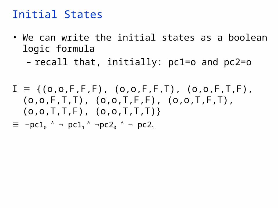
Initial States
• We can write the initial states as a boolean logic formula– recall that, initially: pc1=o and pc2=o
I {(o,o,F,F,F), (o,o,F,F,T), (o,o,F,T,F), (o,o,F,T,T), (o,o,T,F,F), (o,o,T,F,T), (o,o,T,T,F), (o,o,T,T,T)}
pc10 pc11 pc20 pc21

Transition Relation
• We can use boolean logic formulas to encode the transition relation
• We will use two sets of variables:
– Current state variables: pc10,pc11,pc20,pc21,turn,a,b
– Next state variables: pc10’,pc11’,pc20’,pc21’,turn’,a’,b’
• For example, we can write a boolean logic formula for the statement:
cs: a := false;
as follows
pc10 pc11 pc10’ pc11’ a’
(pc20’pc20) (pc21’pc21)(turn’turn)(b’b)
– Call this formula R1c

Transition Relation
• We can write a formula for each statement in the program
• Then the overall transition relation is
R R1o R1w R1c R2o R2w R2c

Symbolic Pre-condition Computation
• Remember the function
EX : 2S 2S
which is defined as:
EX(p) = { s | (s,s’) R and s’ p }• We can symbolically compute pre as follows
EX(p) V’ R p[V’ / V]– V : current-state boolean variables – V’ : next-state boolean variables– p[V’ / V] : rename variables in p by replacing current-
state variables with the corresponding next-state variables
V’ f : existentially quantify out all the variables in V’ from f
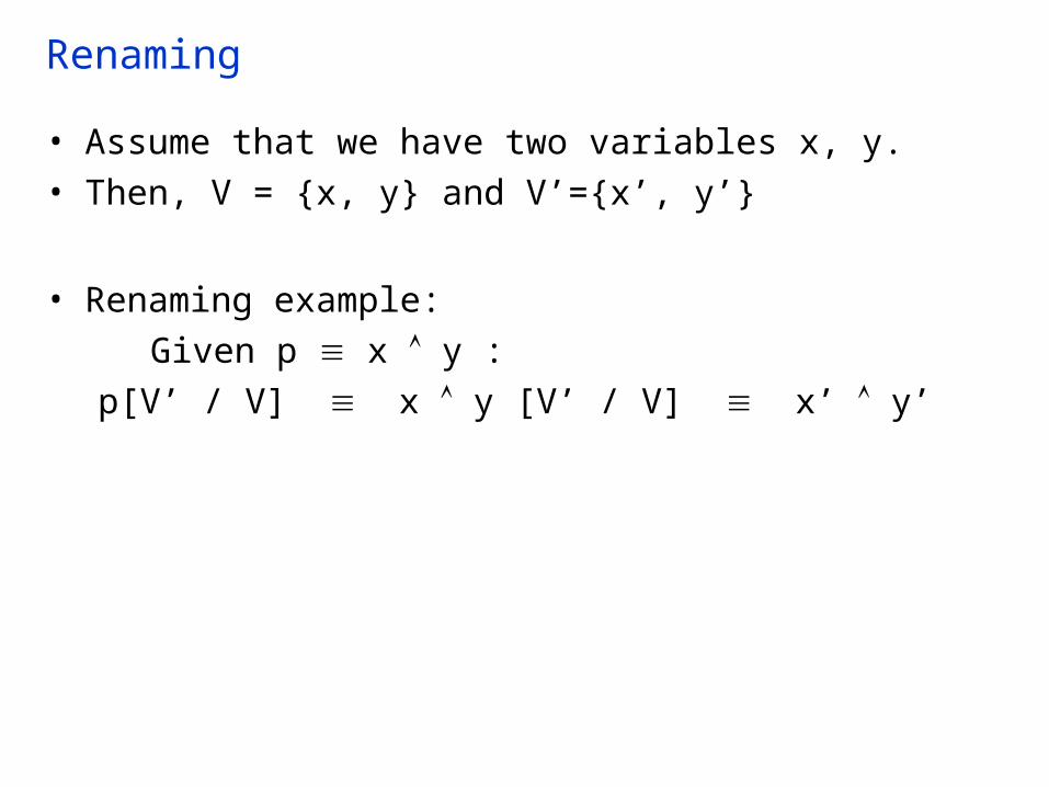
Renaming
• Assume that we have two variables x, y. • Then, V = {x, y} and V’={x’, y’}
• Renaming example:
Given p x y :
p[V’ / V] x y [V’ / V] x’ y’

Existential Quantifier Elimination
• Given a boolean formula f and a single variable vv f f[True/v] f[False/v]i.e., to existentially quantify out a variable, first set it to true
then set it to false and then take the disjunction of the two results
• Example: f x y x’ y’ V’ f x’ ( y’ (x y x’ y’) ) x’ ((x y x’ y’ )[T/y’] (x y x’ y’ )[F/y’]) x’ (x y x’ T x y x’ F ) x’ x y x’ (x y x’)[T/x’] (x y x’)[F/x’]) x y T x y F x y

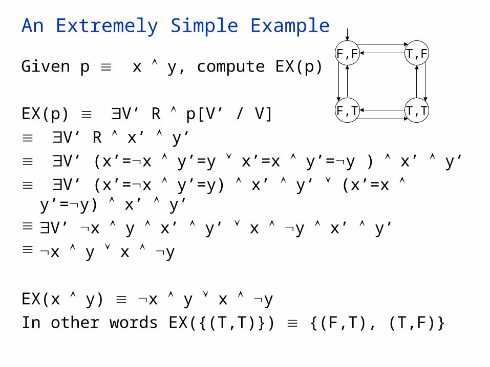
An Extremely Simple Example
Variables: x, y: boolean
Set of states:S = {(F,F), (F,T), (T,F), (T,T)}S True
Initial condition:I x y
Transition relation (negates one variable at a time):R x’=x y’=y x’=x y’=y (= means )
F,T
F,F
T,T
T,F
An Extremely Simple Example
Given p x y, compute EX(p)
EX(p) V’ R p[V’ / V]
V’ R x’ y’
V’ (x’=x y’=y x’=x y’=y ) x’ y’
V’ (x’=x y’=y) x’ y’ (x’=x y’=y) x’ y’ V’ x y x’ y’ x y x’ y’ x y x y
EX(x y) x y x y
In other words EX({(T,T)}) {(F,T), (T,F)}
F,T
F,F
T,T
T,F

An Extremely Simple Example
Let’s compute compute EF(x y)
The fixpoint sequence is
False, xy , xy EX(xy) , xy EX (xy EX(xy) ) , ...
If we do the EX computations, we get:
False, x y , x y x y x y, True
EF(x y) True
In other words EF({(T,T)}) {(F,F),(F,T), (T,F),(T,T)}
F,T
F,F
T,T
T,F
0 1 2 3
1
2
3

An Extremely Simple Example
• Based on our results, for our extremely simple transition system T=(S,I,R) we have
I EF(x y) ( corresponds to implication) hence:
T |= EF(x y)
(i.e., there exists a path from each initial state where eventually x and y both become true at the same time)
I EX(x y) hence:
T |= EX(x y)
(i.e., there does not exist a path from each initial state where in the next state x and y both become true)

An Extremely Simple Example
• Let’s try one more property AF(x y)
• To check this property we first convert it to a formula which uses only the temporal operators in our basis:
AF(x y) EG((x y))
If we can find an initial state which satisfies EG((x y)), then we know that the transition system T, does not satisfy the property AF(x y)

An Extremely Simple Example
Let’s compute compute EG((x y))
The fixpoint sequence is
True, x y, (x y) EX(x y) , …
If we do the EX computations, we get:
True, x y, x y,
EG((x y)) x y
Since I EG((x y)) we conclude that T |= AF(x y)
F,T
F,F
T,T
T,F
0 1 2
0
1

Symbolic CTL Model Checking Algorithm
• Translate the formula to a formula which uses the basis – EX p, EG p, p EU q
• Atomic formulas can be interpreted directly on the state representation
• For EX p compute the precondition using existential variable elimination as we discussed
• For EG and EU compute the fixpoints iteratively

Symbolic Model Checking Algorithm
Check(f : CTL formula) : boolean logic formula
case: f AP return f;
case: f p return Check(p);
case: f p q return Check(p) Check(q);
case: f p q return Check(p) Check(q);
case: f EX p return V’ R Check(p) [V’ / V];

Symbolic Model Checking Algorithm
Check(f) …
case: f EG pY := True; P := Check(p);Y’ := P Check(EX(Y));while (Y Y’) {
Y := Y’; Y’ := P Check(EX(Y));
}return Y;

Symbolic Model Checking Algorithm
Check(f) …
case: f p EU qY := False; P := Check(p); Q := Check(q);Y’ := Q P Check(EX(Y));while (Y Y’) {
Y := Y’; Y’ := Q P Check(EX(Y));
}return Y;

Binary Decision Diagrams (BDDs)
• Ordered Binary Decision Diagrams (BDDs)– An efficient data structure for boolean formula
manipulation– There are BDD packages available: (for example CUDD
from Colorado University)
• BDD data structure can be used to implement the symbolic model checking algorithm discussed above
• BDDs are a canonical representation for boolean logic formulas– given two boolean logic formulas F and G, if F and G are
equivalent their BDD representations will be identical

Binary Decision Trees
Fix a variable order, in each level of the tree branch on the value of the variable in that level
• Examples for boolean formulas on two variables
Variable order: x, y
F
F
F
T
T
T
x
y y
T
F T
T
x y
F
F
F
T
T
F
x
y y
F
F T
T
x y
F
F
F
T
T
F
x
y y
T
F T
T
x
F
F
F
T
T
F
x
y y
F
F T
F
False

BDDs
• Repeatedly apply the following transformations to a binary decision tree:– Remove duplicate terminals– Remove duplicate non-terminals– Remove redundant tests
• These transformations transform the tree to a directed acyclic graph

Binary Decision Trees vs. BDDs
F
F
F
T
T
T
x
y y
T
F T
T
x y
F
F
F
T
T
F
x
y y
F
F T
T
x y
F
F
F
T
T
F
x
y y
T
F T
T
x
F
F
F
T
T
F
x
y y
F
F T
F
False
F
F
F
T
T
T
x
y
F
F
F
T
T
T
x
yF
F T
T
x F

Good News About BDDs
• Given BDDs for two boolean logic formulas F and G
– The BDDs for F G and F G are of size |F| |G| (and can be computed in that time)
– The BDD for F can be computed in and is of size |F| (and can be computed in that time)
– F ? G can be checked in constant time
– Satisfiability of F can be checked in constant time• No, this does not mean that you cane solve SAT in
constant time

Bad News About BDDs
• The size of a BDD can be exponential in the number of boolean variables
• The sizes of the BDDs are very sensitive to the variable ordering. Bad variable ordering can cause exponential increase in the size of the BDD
• There are functions which have BDDs that are exponential for any variable ordering (for example binary multiplication)
• Pre condition computation requires existential variable
elimination– Existential variable elimination can cause an exponential
blow-up in the size of the BDD

BDDs are Sensitive to Variable Ordering
Identity relation for two variables: (x’ x) (y' y)
T
F
F
FT
F
y
y’
F
F
T
T
x
x’ x’
y’
T
TTF
Variable order: x, x’, y, y'
For n variables, 3n+2 nodes
T
F
F
F T
F
x’
y’
F
F
T
T
x
y y
y’
T
T
T
F
Variable order: x, y, x’, y'
For n variables, 3 2n – 1 nodes
x’ x’x’
T
F
F TF
T

SMV [McMillan 93]
• BDD-based symbolic model checker • Finite state• Temporal logic: CTL• Focus: hardware verification
– Later applied to software specifications, protocols, etc.• SMV has its own input specification language
– concurrency: synchronous, asynchronous – shared variables– boolean and enumerated variables– bounded integer variables (binary encoding)
• SMV is not efficient for integers, but it can be fixed– fixed size arrays

Example Mutual Exclusion Protocol
Process 1:while (true) { out: a := true; turn := true; wait: await (b = false or turn = false); cs: a := false;}||Process 2:while (true) { out: b := true; turn := false; wait: await (a = false or turn); cs: b := false;}
Two concurrently executing processes are trying to enter a critical section without violating mutual exclusion
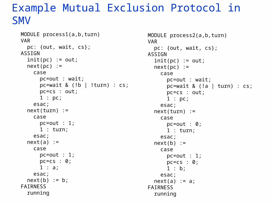
Example Mutual Exclusion Protocol in SMV
MODULE process1(a,b,turn)VAR pc: {out, wait, cs};ASSIGN init(pc) := out; next(pc) := case pc=out : wait; pc=wait & (!b | !turn) : cs; pc=cs : out; 1 : pc; esac; next(turn) := case pc=out : 1; 1 : turn; esac; next(a) := case pc=out : 1; pc=cs : 0; 1 : a; esac; next(b) := b;FAIRNESS running
MODULE process2(a,b,turn)VAR pc: {out, wait, cs};ASSIGN init(pc) := out; next(pc) := case pc=out : wait; pc=wait & (!a | turn) : cs; pc=cs : out; 1 : pc; esac; next(turn) := case pc=out : 0; 1 : turn; esac; next(b) := case pc=out : 1; pc=cs : 0; 1 : b; esac; next(a) := a;FAIRNESS running

Example Mutual Exclusion Protocol in SMV
MODULE mainVAR a : boolean; b : boolean; turn : boolean; p1 : process process1(a,b,turn); p2 : process process2(a,b,turn);SPEC AG(!(p1.pc=cs & p2.pc=cs)) -- AG(p1.pc=wait -> AF(p1.pc=cs)) & AG(p2.pc=wait -> AF(p2.pc=cs))
Here is the output when I run SMV on this example to check the mutual exclusion property
% smv mutex.smv-- specification AG (!(p1.pc = cs & p2.pc = cs)) is true
resources used:user time: 0.01 s, system time: 0 sBDD nodes allocated: 692Bytes allocated: 1245184BDD nodes representing transition relation: 143 + 6
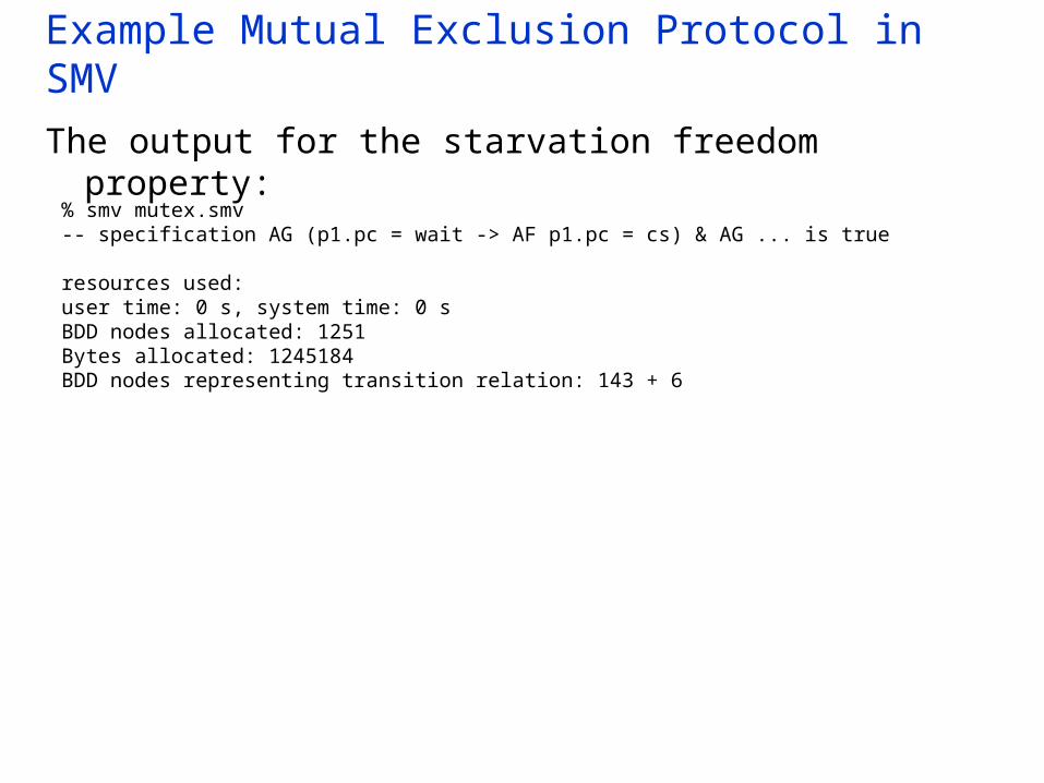
Example Mutual Exclusion Protocol in SMV
The output for the starvation freedom property:
% smv mutex.smv-- specification AG (p1.pc = wait -> AF p1.pc = cs) & AG ... is true
resources used:user time: 0 s, system time: 0 sBDD nodes allocated: 1251Bytes allocated: 1245184BDD nodes representing transition relation: 143 + 6

Example Mutual Exclusion Protocol in SMV
Let’s insert an error
change pc=wait & (!b | !turn) : cs;
to pc=wait & (!b | turn) : cs;

% smv mutex.smv-- specification AG (!(p1.pc = cs & p2.pc = cs)) is false-- as demonstrated by the following execution sequencestate 1.1:a = 0b = 0turn = 0p1.pc = outp2.pc = out[stuttering]
state 1.2:[executing process p2]
state 1.3:b = 1p2.pc = wait[executing process p2]
state 1.4:p2.pc = cs[executing process p1]
state 1.5:a = 1turn = 1p1.pc = wait[executing process p1]
state 1.6:p1.pc = cs[stuttering]
resources used:user time: 0.01 s, system time: 0 sBDD nodes allocated: 1878Bytes allocated: 1245184BDD nodes representing transition relation: 143 + 6
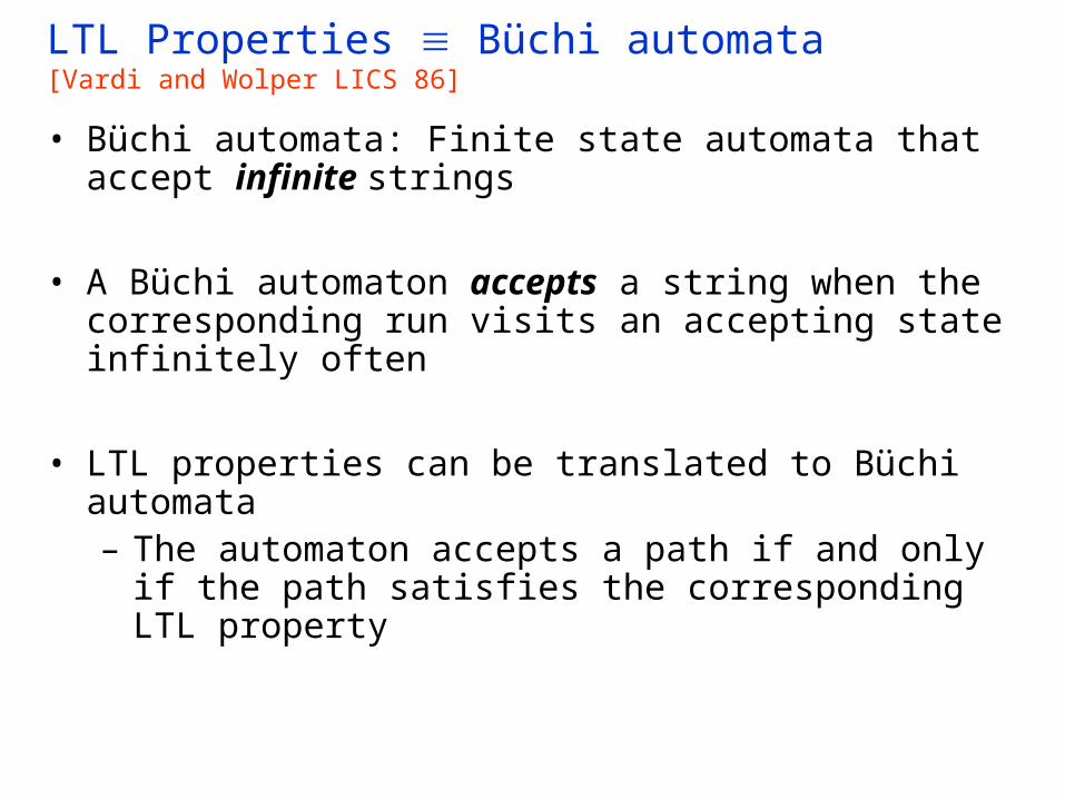
LTL Properties Büchi automata [Vardi and Wolper LICS 86]
• Büchi automata: Finite state automata that accept infinite strings
• A Büchi automaton accepts a string when the corresponding run visits an accepting state infinitely often
• LTL properties can be translated to Büchi automata – The automaton accepts a path if and only if the path
satisfies the corresponding LTL property

LTL Properties Büchi automata
G p p ptrue
F p pptrue
G (F p) p
The size of the property automaton can be exponential in the size of the LTL formula (recall the complexity of LTL model checking)
p
p
p

Büchi Automata
• Given a Buchi automaton, one interesting question is: – Is the language accepted by the automaton empty?
• i.e., does it accept any string?• A Büchi automaton accepts a string when the
corresponding run visits an accepting state infinitely often• To check emptiness:
– Find a cycle which contains an accepting state and is reachable from the initial state
• Find a strongly connected component that contains an accepting state, and is reachable from the initial state
– If no such cycle can be found the language accepted by the automaton is empty

LTL Model Checking
• Generate the property automaton from the negated LTL property
• Generate the product of the property automaton and the transition system
• Show that there is no accepting cycle in the product automaton (check language emptiness)– i.e., show that the intersection of the paths generated by
the transition system and the paths accepted by the (negated) property automaton is empty
• If there is a cycle, it corresponds to a counterexample behavior that demonstrates the bug

LTL Model Checking Example
p,q
p,q
p,q
G q
Each state is labeled with the propositions that hold in that state
Example transition system Property to be verified
Negation of the property
G q F q
Property automaton for the negated property
q qtrue

Buchi automaton forthe transition system(every state is accepting)
p,q
p,q
p,q
p,q
p,q
q qtrue
Property Automaton
1
2
3 4
1 2
Product automaton
p,q
p,q
p,q
p,q
1,1
2,1
3,1
4,2
p,q3,2
p,q
Accepting cycle:
(1,1), (2,1), (3,1), ((4,2), (3,2))

SPIN [Holzmann 91, TSE 97]
• Explicit state model checker• Finite state• Temporal logic: LTL• Input language: PROMELA
– Asynchronous processes – Shared variables – Message passing through (bounded) communication
channels– Variables: boolean, char, integer (bounded), arrays
(fixed size)– Structured data types

SPIN
Verification in SPIN• Uses the LTL model checking approach• Constructs the product automaton on-the-fly
– It is possible to find an accepting cycle (i.e. a counter-example) without constructing the whole state space
• Uses a nested depth-first search algorithm to look for an accepting cycle
• Uses various heuristics to improve the efficiency of the nested depth first search:– partial order reduction– state compression

Example Mutual Exclusion Protocol
Process 1:while (true) { out: a := true; turn := true; wait: await (b = false or turn = false); cs: a := false;}||Process 2:while (true) { out: b := true; turn := false; wait: await (a = false or turn); cs: b := false;}
Two concurrently executing processes are trying to enter a critical section without violating mutual exclusion

Example Mutual Exclusion Protocol in Promela
#define cs1 process1[0]@cs#define cs2 process2[0]@cs#define wait1 process1[0]@wait#define wait2 process2[0]@wait#define true 1#define false 0bool a;bool b;bool turn;init { run process1(); run process2()}proctype process1(){out: a = true; turn = true;wait: (b == false || turn == false);cs: a = false;}proctype process2(){out: b = true; turn = false;wait: (a == false || turn == true);cs: b = false;}

Property automaton generation
% spin -f "! [] (! (cs1 && cs2))"never { /* ! [] (! (cs1 && cs2)) */T0_init: if :: ((cs1) && (cs2)) -> goto accept_all :: (1) -> goto T0_init fi;accept_all: skip}
% spin -f "!([](wait1 -> <>(cs1)))"never { /* !([](wait1 -> <>(cs1))) */T0_init: if :: (! ((cs1)) && (wait1)) -> goto accept_S4 :: (1) -> goto T0_init fi;accept_S4: if :: (! ((cs1))) -> goto accept_S4 fi;}
Concatanate the generated never claims to the end of the specification file

SPIN
• “spin –a mutex.spin” generates a C program “pan.c” from the specification file – This C program implements the on-the-fly nested-depth
first search algorithm– You compile “pan.c” and run it to the model checking
• Spin generates a counter-example trace if it finds out that a property is violated

% mutex1 -awarning: for p.o. reduction to be valid the never claim must be stutter-closed(never claims generated from LTL formulae are stutter-closed)(Spin Version 3.4.17 -- 9 September 2002) + Partial Order Reduction
Full statespace search for: never-claim + assertion violations + (if within scope of claim) acceptance cycles + (fairness disabled) invalid endstates - (disabled by never-claim)
State-vector 28 byte, depth reached 27, errors: 0 36 states, stored 11 states, matched 47 transitions (= stored+matched) 0 atomic stepshash conflicts: 0 (resolved)(max size 2^18 states)
1.493 memory usage (Mbyte)
unreached in proctype :init: (0 of 3 states)unreached in proctype process1 (0 of 5 states)unreached in proctype process2 (0 of 5 states)

Infinite State Model Checking
• Model checking is undecidable if the data domains are unbounded– For example if you have unbounded integer variables
• Symbolic model checking can be extended to infinite domains– Instead of Boolean logic, use linear arithmetic formulas
to encode unbounded integers or reals– However, the fixpoints are not guaranteed to converge

Infinite State Model Checking
There are infinite state symbolic model checkers which use conservative approximation techniques such as widening
• HyTech: for verification of hybrid systems. – HyTech verifies properties of systems with both discrete
components (specified as state machines) and continuous components (specified with differential equations)
• Action Language Verifier (developed by my research group) for verification of systems with unbounded integer variables – There is an extension of Action Language Verifier which
uses shape analysis to verify concurrent linked lists

Conservative Approximations
• Given a temporal logic property p, compute a lower ( p ) or an upper ( p+ ) approximation to the truth set of the property
• Model checker can give three answers:
II pppp
“The property is satisfied”
II pp
“I don’t know”
“The property is false and here is a counter-example”
II pp ppsates whichsates whichviolate the violate the propertyproperty
pp++
pp
Bounded Model Checking
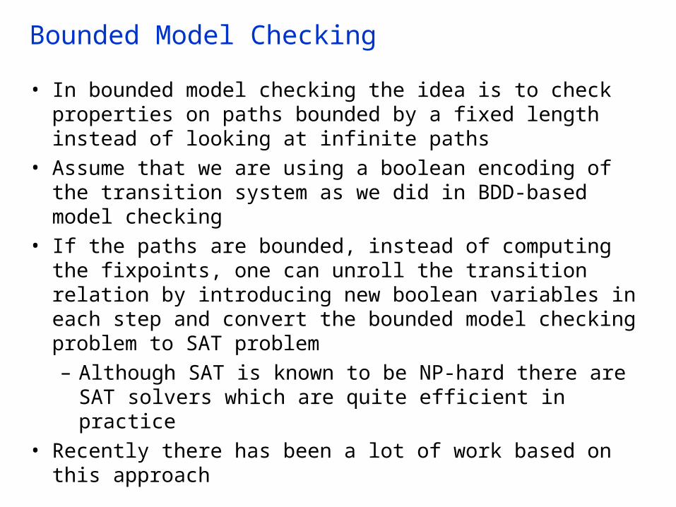
• In bounded model checking the idea is to check properties on paths bounded by a fixed length instead of looking at infinite paths
• Assume that we are using a boolean encoding of the transition system as we did in BDD-based model checking
• If the paths are bounded, instead of computing the fixpoints, one can unroll the transition relation by introducing new boolean variables in each step and convert the bounded model checking problem to SAT problem– Although SAT is known to be NP-hard there are SAT
solvers which are quite efficient in practice• Recently there has been a lot of work based on this
approach

Timed Automata
There are some classes of infinite state systems for which model checking is decidable
• Timed automata: Finite state control + clocks (real valued) – Clocks increase with a fixed rate and they can be reset
to zero when a transition is taken• Model checking timed automata is decidable
– It is possible to construct a finite state abstraction which preserves the temporal logic properties
• A lot of applications in real time systems– There are model checking tools available for timed
automata

Push-down Automata
Another class of infinite state systems for which model checking is decidable
• Push-down automata: Finite state control + one stack• LTL model checking for push-down automata is decidable• This may sound like a theoretical result but it has been the
basis of some promising research on model checking programs– A program with finite data domains which uses recursion
can be modeled as a pushdown automaton

Model Checking Programs
• Recently researchers developed tools for model checking programs– These model checkers work directly on programs, i.e.,
their input language is the programming language• SLAM project at Microsoft Research
– Symbolic model checking for C programs, unbounded recursion, no concurrency
• Uses predicate abstraction and BDDs• Java Path Finder (JPF) at NASA Ames
– Explicit state model checking for Java programs, bounded search, bounded recursion, handles concurrency
• Verisoft from Bell Labs– C programs, handles concurrency, bounded search,
bounded recursion, stateless search

Model Checking Programs
• Program model checking tools generally rely on automated abstraction techniques to reduce the state space of the system such as: – Abstract interpretation– Predicate abstraction
• If the abstraction is conservative then, if there is no error in the abstracted program we can conclude that there is no error in the original program
• In general the problem is to construct a finite state model from the program such that the errors or absence of errors can be demonstrated on the finite state model– Model extraction problem– BANDERA: A tool for extracting finite state models from
programs

Abstract Interpretation Example
• Assume that we have two integer variables x and y• Define an abstract domain for integers
– For example: {, Т, neg, zero, pos}• Define abstraction and concretization functions between the
integer domain and this abstract domain• Interpret integer expressions in the abstract domain
• Abstraction will reduce the state space significantly, however it will also introduce spurious behaviors which are not in the original system
if (y == 0) { x = 2; y = x;}
if (y == zero) { x = pos; y = x;}

Predicate Abstraction
• An automated abstraction technique which can be used to reduce the state space of a program
• The basic idea in predicate abstraction is to remove some variables from the program by just keeping information about a set of predicates about them
• For example a predicate such as x = y maybe the only information necessary about variables x and y to determine the behavior of the program– In that case we can just store a boolean variable which
corresponds to the predicate x = y and remove variables x and y from the program
– Predicate abstraction is a technique for doing such abstractions automatically

Predicate Abstraction
• Given a program and a set of predicates, predicate abstraction abstracts the program so that only the information about the given predicates are preserved
• The abstracted program adds nondeterminism since in some cases it may not be possible to figure out what the next value of a predicate will be based on the predicates in the given set
• One needs an automated theorem prover to compute the abstraction

Predicate Abstraction, Simple Example
• Assume that we have again two integer variables x,y• We want to abstract the program based on a single
predicate x=y which we will represent as the boolean variable B in the abstract program
Concrete Statement y := y + 1
Abstract Statement
y := y + 1 {x = y}
y := y + 1 {x y} {x y + 1}
{x = y + 1}
Step 1: Calculate the precondition
Step 2: Rewrite in terms of predicatesStep 2a: Use Decision Procedures
x = y x = y + 1 ? No
x y x = y + 1 ? No
x = y x y + 1 ? Yes
x y x y + 1 ? No
{x = y + 1} y := y + 1 {B}{B} y := y + 1 {~B}
Step 3: Abstract Code
IF B THEN B := false ELSE B := true | false
(Example taken from Matt Dwyer’s slides)

Predicate Abstraction + Model Checking Push Down Automata
• Predicate abstraction combined with results on model checking pushdown automata led to some promising tools– SLAM project at Microsoft Research for verification of C
programs– This tool is being used to verify device drivers at
Microsoft• The main idea:
– Use predicate abstraction to obtain finite state abstractions of a program
– A program with finite data domains and recursion can be modeled as a pushdown automaton
– Use results on model checking push-down automata to verify the abstracted (recursive) program

Java Path Finder
• Program checker for Java• Properties to be verified
– Properties can be specified as assertions• static checking of assertions
– It can also verify LTL properties• Implements both depth-first and breadth-first search and
looks for assertion violations statically• Uses static analysis techniques to improve the efficiency of
the search• Requires a complete Java program

Java Path Finder, First Version
• First version – A translator from Java to PROMELA– Use SPIN for model checking
• Since SPIN cannot handle unbounded data– Restrict the program to finite domains
• A fixed number of objects from each class• Fixed bounds for array sizes
• Does not scale well if these fixed bounds are increased
• Java source code is required for translation

Java Path Finder, Current Version
• Current version of the JPF has its own virtual machine: JPF-JVM– Executes Java bytecode
• can handle pure Java but can not handle native code– Has its own garbage collection– Stores the visited states and stores current path – Offers some methods to the user to optimize verification
• Traversal algorithm – Traverses the state-graph of the program– Tells JPF-JVM to move forward, backward in the state space, and evaluate the assertion
• The rest of the slides on the current version of JPF

Storing the States
• JPF implements a depth-first search on the state space of the given Java program– To do depth first search we need to store the visited
states• There are also verification tools which use stateless
search such as Verisoft• The state of the program consists of
– information for each thread in the Java program• a stack of frames, one for each method called
– the static variables in classes• locks and fields for the classes
– the dynamic variables (fields) in objects• locks and fields for the objects

Storing States Efficiently
• Since different states can have common parts each state is divided to a set of components which are stored separately– locks, frames, fields
• Keep a pool for each component– A table of field values, lock values, frame values
• Instead of storing the value of a component in a state store an index at which the component is stored in the table in the state– The whole state becomes an integer vector
• JPF collapses states to integer vectors using this idea

State Space Explosion
• State space explosion if one of the major challenges in model checking
• The idea is to reduce the number of states that have to be visited during state space exploration
• Here are some approaches used to attack state space explosion– Symmetry reduction
• search equivalent states only once – Partial order reduction
• do not search thread interleavings that generate equivalent behavior
– Abstraction• Abstract parts of the state to reduce the size of the
state space

Symmetry Reduction
• Some states of the program may be equivalent– Equivalent states should be searched only once
• Some states may differ only in their memory layout, the order objects are created, etc. – these may not have any effect on the behavior of the
program• JPF makes sure that the order which the classes are
loaded does not effect the state – There is a canonical ordering of the classes in the
memory

Symmetry Reduction
• A similar problem occurs for location of dynamically allocated objects in the heap– If we store the memory location as the state, then we
can miss equivalent states which have different memory layouts
– JPF tries to remedy this problem by storing some information about the new statements that create an object and the number of times they are executed

Partial Order Reduction
• Statements of concurrently executing threads can generate many different interleavings– all these different interleavings are allowable behavior of
the program• A model checker has to check all possible interleavings that
the behavior of the program is correct in all cases – However different interleavings may generate equivalent
behaviors• In such cases it is sufficient to check just one interleaving
without exhausting all the possibilities– This is called partial order reduction

class S1 { int x;}class FirstTask extends Thread { public void run() { S1 s1; int x = 1; s1 = new S!(); x = 3;}}
class Main { public static void main(String[] args) { FirstTask task1 = new FirstTask(); SecondTask task2 = new SecondTask(); task1.statr(); task2.start();}}
class S2 { int y;}class SecondTask extends Thread { public void run() { S2 s2; int x = 1; s2 = new S2(); x = 3;}}
state space search generates 258 stateswith symmetry reduction: 105 stateswith partial order reduction: 68 stateswith symmetry reduction + partial order reduction : 38 states
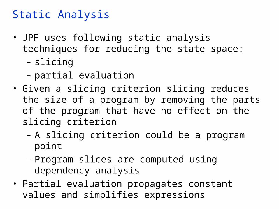
Static Analysis
• JPF uses following static analysis techniques for reducing the state space:– slicing– partial evaluation
• Given a slicing criterion slicing reduces the size of a program by removing the parts of the program that have no effect on the slicing criterion– A slicing criterion could be a program point– Program slices are computed using dependency
analysis• Partial evaluation propagates constant values and simplifies
expressions

Abstraction and Restriction
• JPF also uses abstraction techniques such as predicate abstraction to reduce the state space
• Still, in order to check a program with JPF, typically, you need to restrict the domains of the variables, the sizes of the arrays, etc.
• Abstraction over approximates the program behavior– causes spurious counter-examples
• Restriction under approximates the program behavior– may result in missed errors
• If both under and over approximation techniques are used then the resulting verification technique is neither sound nor complete– However, it is still useful as a debugging tool and it is
helpful in finding bugs

JPF Java Modeling Primitives
• Atomicity (used to reduce the state space)– beginAtomic(), endAtomic()
• Nondeterminism (used to model non-determinism caused by abstraction)– int random(int); boolean randomBool(); Object randomObject(String cname);
• Properties (used to specify properties to be verified)– AssertTrue(boolean cond)

Annotated Java Code for a Reader-Writer Lock
import gov.nasa.arc.ase.jpf.jvm.Verify;class ReaderWriter {private int nr;private boolean busy;private Object Condr_enter;private Object Condw_enter;public ReaderWriter() { Verify.beginAtomic(); nr = 0; busy=false ; Condr_enter =new Object(); Condw_enter =new Object(); Verify.endAtomic();}public boolean read_exit(){ boolean result=false; synchronized(this){ nr = (nr - 1); result=true; } Verify.assertTrue(!busy || nr==0 ); return result;}
private boolean Guarded_r_enter(){ boolean result=false; synchronized(this){ if(!busy){nr = (nr +
1);result=true;}} return result;}public void read_enter(){ synchronized(Condr_enter){ while (! Guarded_r_enter()){
try{Condr_enter.wait();} catch(InterruptedException e){}
}} Verify.assertTrue(!busy || nr==0 );}private boolean Guarded_w_enter(){…}public void write_enter(){…}public boolean write_exit(){…}};

JPF Output>java gov.nasa.arc.ase.jpf.jvm.Main rwmain
JPF 2.1 - (C) 1999,2002 RIACS/NASA Ames Research CenterJVM 2.1 - (C) 1999,2002 RIACS/NASA Ames Research Center
Loading class gov.nasa.arc.ase.jpf.jvm.reflection.JavaLangObjectReflectionLoading class gov.nasa.arc.ase.jpf.jvm.reflection.JavaLangThreadReflection============================== No Errors Found==============================
-----------------------------------States visited : 36,999Transitions executed : 68,759Instructions executed: 213,462Maximum stack depth : 9,010Intermediate steps : 2,774Memory used : 22.1MBMemory used after gc : 14.49MBStorage memory : 7.33MBCollected objects : 51Mark and sweep runs : 55,302Execution time : 20.401sSpeed : 3,370tr/s-----------------------------------
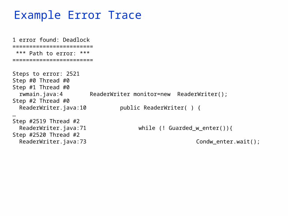
Example Error Trace
1 error found: Deadlock======================== *** Path to error: ***========================
Steps to error: 2521Step #0 Thread #0Step #1 Thread #0 rwmain.java:4 ReaderWriter monitor=new ReaderWriter();Step #2 Thread #0 ReaderWriter.java:10 public ReaderWriter( ) {…Step #2519 Thread #2 ReaderWriter.java:71 while (! Guarded_w_enter()){Step #2520 Thread #2 ReaderWriter.java:73 Condw_enter.wait();

THE END THE END THE END THE END THE END