1

Model-based General Arcing Fault Detection inMedium Voltage Distribution System (V1.0)

Wenhai Zhang

Abstract—Arcing fault is a special fault in MV(Mediumvoltage) distribution system, including high current arcing faultand low current arcing fault, which may cause shock hazard,apparatuses failure and wild fire. In this paper, a model basedgeneral arcing fault detection method is proposed in whichthe binary hypothesis test is utilized. Firstly, a detailed arcingfault model considering voltage drop on the line is derived andgeneral disturbance model in distribution system is proposed.Then the procedures of arcing fault detection using voltageand current waveforms measured at substation are introduced,involving disturbance current calculation, parameters estimationusing two assumed models, estimation errors calculation anddecision making. Arcing fault is detected when the measuredvoltage and current match the arcing fault model better than thegeneral disturbance model. The method is tested on standard testsystem using PSCAD/EMTDC considering different arcing faultscenarios and disturbances. MATLAB is used for method imple-mentation. Simulation results show that the detection method isnot affected by fault distance, fault resistance and load currentwhich is accurate and robust.

Index Terms—Arcing fault, Incipient fault, High impedancearcing fault, Model based, MV distribution system, Binaryhypothesis test.

I. INTRODUCTION

ARC is a continuous luminous discharge of electricityacross an insulating medium which is changed into a

conducting medium. It can produce large number of heat inshort time which is dangerous for the safety of human beingsand power system apparatuses. For the arcing fault in MVdistribution system, it may cause explosion in undergroundcable[1], lead to potential hazard to human beings and po-tential fire hazards [2], especially the arcing fault caused bydown conductor in contact with a high impedance surfacesuch as asphalt road, macadam, grass or sand[3]. It is theimportant feature of instantaneous fault which is useful forautoreclosure[4][5]. It is also the symbol of incipient faultin distribution system[6], especially the incipient fault inunderground cable[7]. So the arcing fault is very importantfor the safety and reliability of MV distribution system.

Arc can be divided into high-current arc and low-currentarc[8]. Arcing fault in MV distribution system also can bedivided into high-current arcing and low-current arcing fault.However, the conventional over-current protection in MVdistribution system is time-inverse. The high-current arcingfault with short duration and low-current arcing fault cannot be

This work was supported in part by China Scholarship Council under Grant20140624005 and ”Youth Software Creative Engineering” from TechnologicalOffice of SiChuan under Grant 2015121.

W. Zhang is with the School of Electrical Engineering and Information,Sichuan University, Chengdu, China, (e-mail: zhangwh1989@163.com).

detected by conventional over-current protection. For example,incipient fault in underground cable, although its fault currentcan reach several kA, it may only last several cycles for theself-clearing feature[9]. And high impedance arcing fault inoverhead line, its fault is only tens ampere which is not largeenough to trigger the conventional over-current relays[10].

In the past decades, there are several methods have beenproposed for the two types arcing fault detection separately.For high current arcing fault detection, the arcing fault isrecognized as harmonic source and some time-domain orfrequency-domain methods are proposed for voltage analysisfor arcing fault detection[4][5][12]. However, the voltagefeature measured at substation is weakened by large voltagedrop on the line because fault current is very large, also thefault distance is unknown before arcing fault is detected. Forlow current arcing fault, it is also called high impedancearcing fault in previous study. An extensive review of detectionmethods are summarized in [3]. The detection methods can bebroadly classified into frequency domain, time domain, hybridalgorithms and expert systems[10][13][14]. However, the faultcurrent is always between 20 A to 75 A which is smallerthan the load current(hundreds A). So the detection method isaffected by the load current heavily. More importantly, there isno definite division between two types arcing fault, it is hardto choose the proper method especially when the fault currentis between two types fault and there is no method can detecttwo types arcing fault simultaneously

In this paper, a steady state model based general arcing faultdetection method is proposed. The binary hypothesis test isutilized for the arcing fault detection which has been utilized incontrol system failure detection [15][16]. An accurate generalarcing fault model is proposed derived, in which the voltagedrop on line and load current are considered in the model.Also, a general no-arc disturbance model is proposed to modelload switching, motor starting and constant impedance fault.The proposed method can detect the arcing fault accurately us-ing the voltage and current waveforms measured at substation.It is tested on modified IEEE 13-node test feeders simulatedusing PSCAD/EMTDC.

The paper is divided into five sections. Section I introducesthe background of arcing fault detection. Section II presentsthe idea of the binary hypothesis test for arcing fault detec-tion.In section III, the arcing fault model and general no-arcdisturbances model for arc detection are presented. In sectionIV, the procedures of arcing fault detection are introduced indetail, including disturbance current calculation, parametersestimation, MSE(mean square error) calculation and detectiondecision making. Section V describes the arcing fault detection

2

Modeldesign

Theoretical analysis

Calculate if

Waveforms of vs and is Model input Parameters

estimationNMSE

calculationDecision making

Fig. 1. The framework of model based arcing fault detection.

simulation results. Finally, conclusions are drawn in sectionVI.

II. PROBLEM DESCRIPTION

For arcing fault detection, it can be described as discrim-inating arcing fault from other disturbances. There are twopossible detection results, one is that it is arcing fault, anotheris that it is not arcing fault. So arcing fault detection can berecognized as binary hypothesis test problem. Two hypothesesare denoted H0 and H1 which is stated as follows:

H0: It is arcing fault.H1: It is not arcing fault.

in which the observer is voltage and current waveformsmeasured at substation.

In order to test which hypothesis is correct, the modelbased parameters estimation is proposed for testing. The ideaof the detection is as shown in Fig. 1. Firstly, the arcingfault and no-arc model expressed by voltage and currentmeasured at substation are conducted. Then estimate the modelparameters based on the two hypothesis models separately. Thelikelihood-ratio test(LRT) is used for testing. Voltage meansquare error(MSE) is figured out to evaluate the two hypothesismodels. At last compare two MSEs to make the decision.

III. MODEL INTRODUCTION

A. Arcing Fault Model

The research on arc model have been conducted for severaldecades and many arc models have been proposed for differentmotivations, circuit-breaker arc analysis, arc energy calculationand arcing fault analysis. In this section, the arc model for faultanalysis is introduced.

In this paper, the Kizilcay’s arc model is utilized for arcingfault detection and simulation which is a dynamic arc modeland derived from the viewpoint of control system theory basedon the energy balance in the arc column [17]. The model hasbeen tested in [18] and it is proved accurate, it also has beenutilized in many arcing fault analysis [19][20][21][22]. Thearc model is introduced as follows:

Rarc(t) =1

g(t)(1)

dg(t)

dt=

1

τ(

|if (t)|u0 + r0|if (t)|

− g(t)) (2)

whereRarc is arc resistance,g is arc conductance,if is arc current,

Rarc

vf

R0

if

Fig. 2. Arcing fault model in distribution system.

vf

Motor starting

model

R

L

vf

Load switching

model

R

vf

Constant impedance

fault model

R

L

if ifif

vf

R

L

if

General

R-L model

Fig. 3. The no-arc disturbance models in distribution system, (a) is the modelsof different disturbances, including motor starting, constant impedance faultand load switching (b) is the general no-arc disturbance model, R-L model.

u0 is characteristic arc voltage,r0 is characteristic arc resistance,τ is arc time constant.For arcing fault in distribution system, the arcing fault

can be modeled using an arc model series with a constantresistance R0, as shown in Fig. 2. When series resistance is 0,it is recognized as pure arcing fault which is always occurs inunderground cable, when R0 is large, it is recognized as lowcurrent arcing fault. The model has been used in [19] for treecontacting arcing fault analysis and is verified by the lab test.So the general arcing fault model can be written as follows:

vf (t) = if (t) ·R0 + if (t) ·Rarc (3)

where vf and if are arc voltage and current in arcing faultmodel as shown in Fig. 2, R0 is constant resistance.

B. The General No-arc Disturbance Model

In order to discriminate arcing fault from other similar dis-turbances, the no-arc disturbances such as constant impedancefault, motor starting and load switching are introduced in thissection. The models of these disturbances are shown in Fig.3(a). It is noted that although the motor starting model is adynamic model, in fact it can be recognized as static model inshort time (two cycles). So the models of these disturbancescan be recognized as a series R-L model as shown in Fig. 3(b).Then the no-arc general model can be described as follows:

vf (t) = if (t) ·R+ L · dif (t)

dt(4)

where R and L are the resistance and inductance of distur-bance as shown in Fig. 3.

C. General Model Considering Voltage Drop

In distribution system, there is only one measurement whichlocates at substation. But the models introduced above are

3

expressed by the voltage and current at disturbance location.So we need to take the voltage drop on line and load currentinto consideration. And express arcing fault model and no-arc disturbance model in the form of voltage and currentmeasured at substation. As shown in Fig. 4, a detailed modelis introduced in which the voltage drop ∆v and load branchare considered. Then voltage measured at substation vs can bewritten by ∆v and vf as follows:

vs(t) = ∆v(t) + vf (t). (5)

The ∆v can be written using the load branch current andline impedance as follows:

∆v(t) = is1(t) · Zl1 + is2(t) · Zl2 + ...+ isn(t) · Zln

= is1(t) ·Rl1 + is2(t) ·Rl2 + ...+ isn(t) ·Rln

+ Ll1 ·dis1(t)

dt+ Ll2 ·

dis2(t)

dt+ ...+ Lln ·

disn(t)

dt(6)

where is1(t), is2(t) ... isn(t) are the currents flow through thefault path, Zl1, Zl2 ... Zln are line section impedance whichare composed of resistance component Rln and inductancecomponent Lln, as shown in Fig. 4(a). Assuming all thecurrents flow through the fault path can be written as follows:

is1(t) = k1 · is(t)is2(t) = k2 · is(t)

...

isn(t) = kn · is(t) (7)

where k1, k2, ..., kn are constant. Then ∆v(t) can be rewrittenas follows:

∆v(t) =(k1 ·Rl1 + k2 ·Rl2 + ...+ kn ·Rln) · is(t)

+ (k1 · Ll1 + k2 · Ll2 + ...+ kn · Lln) · dis(t)dt

.

(8)

Suppose:

Req = k1 ·Rl1 + k2 ·Rl2 + ...+ kn ·Rln

Leq = k1 · Ll1 + k2 · Ll2 + ...+ kn · Lln. (9)

Then ∆v(t) can be written as follows:

∆v(t) = Req · is(t) + Leq ·dis(t)

dt(10)

where Req and Leq are the equivalent resistance and induc-tance for ∆v(t) calculation, as shown in Fig. 4(b).

The general model for all disturbances considering voltagedrop on the line using measurement at substation can bewritten as follows:

vs(t) = Req · is(t) + Leq ·dis(t)

dt+ vf (t) + n(t) (11)

where n(t) is Gauss noise including model error, vf (t) isdisturbance voltage which can be expressed by disturbancemodel, including arcing fault model and R-L model, as shownin (3) and (4).

Zs1 Zs2 Zsn

iload1 iload2 iloadn

Zloadm

iloadm

is1 is2 isn

vf

Distu

rbance

if

vs

Bus…...

Zload1 Zload2 Zloadn

∆v

Zload

iload

is

vf

(b)

Leq Req

if

vs

(a)

Bus

Distu

rbance

Fig. 4. The accurate model for arcing fault detection, (a) is the detailed modelconsidering load branch, (b) is the equivalent simplified model.

D. Problem Definition

In section II, the idea of binary hypothesis test for arcingfault detection has been introduced. The arcing fault modeland no-arc model base parameters estimation are used totest the hypothesis. If it’s arcing fault, the disturbance wouldmatch the arcing fault model very well with low voltageMSE. If it is not, the disturbance would match the R-Lmodel well. Combining the models introduced above, the twohypotheses for arcing fault detection can be defined as follows:

H0 : The disturbance is arcing fault, the model is shown asfollows:vs(t) = Req · is(t) + Leq ·

dis(t)

dt+ if (t) ·R0 +

if (t)

g(t)+ n(t)

dg(t)

dt=

1

τ

(|if (t)|

u0 + r0|if (t)|− g(t)

)(12)

where (Req , Leq , R0, τ , u0, r0) are the parameters need toestimate.

H1 : The disturbance is not arcing fault and it’s general R-Lmodel based disturbance. The model is shown as follows:

vs(t) = Req · is(t)+Leq ·dis(t)

dt+R · if (t)+L · dif (t)

dt+n(t)

(13)where (Req , Leq , R, L) are the parameters need to estimate.

If the decision is in favor of hypothesis H0, the disturbanceis arcing fault. In order to identify which hypothesis is better,two models are used for parameters estimation separately, thencompare the estimation error to make decision which will beintroduced in the next section.

IV. PARAMETERS ESTIMATION FOR ARCING FAULTDETECTION

In this section, the procedures for arcing fault detection us-ing voltage and current measured at substation are introducedin detail, including disturbance current estimation, parametersestimation, voltage MSE calculation and decision making.

4

A. Disturbance Current if Calculation

As introduced in section III, two hypothesis models havebeen introduced in (12) and (13). As shown in equation,apart from the parameters need to estimate, vs and is aremeasured at substation, so the disturbance current if is neededto calculate out before parameters estimation. Assuming theload is constant impedance Zload, as shown in Fig. 4(b), thenthe sum of load impedance and line impedance can be esti-mated by the pre-disturbance current and voltage measured atsubstation. Then the relation between disturbance current andother parameters can be built, and if can be expressed usingduring-disturbance voltage vsd measured at substation andReq , Leq . The procedures of disturbance current calculationincludes following three steps:

Step 1) Estimate the sum of line impedance and Zload

using pre-disturbance current and voltage based on Ohm’s lawwritten as Z ′ which include R′ and L′. Then the Rload andLload can be expressed as:

Rload = R′ −Req

Lload = L′ − Leq

(14)

Step 2) As shown in Fig. 4(b), the relationship betweenZload and during-disturbance voltage and current vs, is. It canbe written in the form of differential equation as follows:

vs(n) = is(n)·Req+Leq ·dis(n)

dt+il(n)·Rload+Lload ·

dil(n)

dt(15)

Put (14) into (15), and write the dil(n)/dt in the form ofdifference equation, then il(n) can be figured out:

il(n) =[vs(n)− is(n) ·Req − Leq · dis(n)/dt] ·∆t

(R′ −Req) ·∆t+ L′ − Leq

+(L′ − Leq) · il(n− 1)

(R′ −Req) ·∆t+ L′ − Leq(16)

where the current differential dis(n)/dt can be figured out inthe form of difference equation as follows:

dis(n)

dt=is(n)− is(n− 1)

∆t. (17)

Assuming il(1) = 0, when n≥2, il(n) can be figured outbased on (16) and g(1) as follows:

il(n) =

n∑j=2

A(j) ·Bn−j +Bn−1 · il(1) (18)

where A and B are:A(n) =

[vs(n)− is(n) ·Req − Leq · dis(n)/dt] ·∆t(R′ −Req) ·∆t+ L′ − Leq

B =L′ − Leq

(R′ −Req) ·∆t+ L′ − Leq.

Step 3) Then the disturbance current if can be calculatedout based on KCL as follows:

if (n) = is(n)− il(n). (19)

which is the function of (Req , Leq).

B. The Model Based Parameters Estimation

For parameters estimation, the lsqcurvefit function in MAT-LAB is used which is based on least-square curve fittingmethod. The parameters estimation problem is described asoptimization problem and the objective function is as follows:

minx

N∑n=1

[F (x, data(n))− vs(n)]2 (20)

where N is the total number of sampling point for calculation,x is the parameters need to estimate (Req , Leq , R0, τ , u0, r0)for arcing fault model, and (Req , Leq , R, L) for R-L model;data is the known parameters (is, if , dis/dt) for arcing faultmodel, and (is, if , dis/dt, dif/dt) for R-L model, F (x, data)is vs calculation which have been introduced in (12) and (13).

The lsqcurvefit function in MATLAB is utilized in the formof x = lsqcurvefit(F (x, data), x0, data, vs, lb, ub), wherex0 is the initial value of the estimate parameters, lb and ub arethe lower and upper bounds of the estimate parameters. Thenwe will introduce the F (x, data) for two models in detail. ForR-L model, F (x, data) can be figured out based on the x and(is, if , dis/dt, dif/dt) as shown in (13) in which is is themeasured current and if is calculated out in (19). The currentdifferential dis/dt and dif/dt can be figured out in the formof difference equation, such as:

dis(n)

dt=is(n)− is(n− 1)

∆t. (21)

For arcing fault model, it is a dynamic model with dif-ferential equation as shown in (12). So we rewrite the arcconductance calculation in the form of difference equation asfollows:

g(n)− g(n− 1)

∆t=

1

τ

(|if (n)|

u0 + r0|if (n)|− g(n)

). (22)

Then arc conductance can be figured out as follows:

g(n) =∆t · |if (n)|

(τ + ∆t) · (u0 + r0|if (n)|)+τ · g(n− 1)

τ + ∆t. (23)

Assuming g(1) = if (1)/vs(1), when n≥2, g(n) can befigured out based on (23) and g(1) as follows:

g(n) =

n∑j=2

P (j) ·Qn−j +Qn−1 · g(1) (24)

where P and Q are:P (n) =

∆t · |if (n)|(τ + ∆t) · (u0 + r0|if (n)|)

Q =τ

τ + ∆t

(25)

Put 24 into 12, the F (x, data) for arcing fault model canbe calculated out. Then the unknown parameters x can beestimated using lsqcurvefit in MATLAB, the ranges of theparameters would be introduced in the simulation. For arcingfault model, the estimated parameters are written as (Req , Leq ,R0, τ , u0, r0). The estimated parameters using R-L model arewritten as (Req , Leq , R, L).

5

Start

Estimate load impedance Zload.

Estimate the parameters of the

two models using lsqcurvefit.

Calculate earc and enon-arc using (17) and (18).

Parameters

estimation

and MSE

calculation

Decision

making

Calculate disturbance current if using (11)-(12).

earc < enon-arc?

It’s an arcing fault.

N

Y

Disturbance

current

calculation

Fig. 5. The detailed procedures for arcing fault detection.

C. The Voltage MSE Calculation

In this section, the voltage MSE calculation is introducedwhich is the index to evaluate the match degree between mea-sured signal and assumed disturbance model. Firstly, vs canbe calculated out based on estimated parameters and knownparameters as introduced in the last section, the functionF (x, data) is used again for calculation. Then the MSE ofvs can be calculated out based on measured vs and estimatedvs as follows:

MSE =

N∑n=1

[vs(n)− vs(n)]2. (26)

It is noted that there are two MSEs for every disturbance,then we use MSEarc and MSERL to represent the estimationerror of two models separately.

D. Decision Making

In order to justify the disturbance is arcing fault or not, wecompare MSEarc and MSERL to make the decision. If the MSEis small, it means the disturbance match the model well. Thedecision is made as follows:

H0 : MSEarc < MSERL

H1 : MSERL < MSEarc.(27)

The detailed procedures for the model based arcing faultdetection are shown in Fig. 5.

V. SIMULATION STUDIES

In this section, large number of disturbances produced byPSCAD/EMTDC are used to verify the proposed model basedgeneral arcing fault detection method. A modified IEEE 13-node 25kV test system considering underground cable andoverhead line is utilized, as shown in Fig. 6. Different kinds

650

632 633 634645

675692

680652

684611 671

Fault location

1.3 km

2.6 km 7.6 km3.2 km

5.3 km4.2 km7.2 km

9.1 km4.2 km

3.3 km

4.1 km646

5.6 km

M

MMotor

starting location

MM

M

Load switching

location

Voltage and current measurement

25kV BUS

Underground

cableOverhead line

Fig. 6. Modified IEEE-13 node test feeder.

of disturbances, including load switching, constant impedancefault, and motor starting are considered in the simulation. Thelocation of the disturbances are shown in figure, the parametersof the disturbances and simulation results will be introducedfollowing sections.

A. High Current Arcing Fault

For high current arcing fault in distribution system, it alwaysoccurs in underground cable with low fault resistance, node645, 632, 633, 634 are considered as fault node as shown inFig. 6. Based on the arcing fault model introduced in section II,the R0 is zero for this type arcing fault. In [24], the ranges ofarc parameters (τ , u0, r0) are introduced. Combining the pre-vious lab test and field test in underground cable[25][26][27],the arc parameters are summarized as follows: τ : 0.05∼0.4ms,u0: 300∼4000V, r0: 0∼0.015ohm. For the large number ofsimulation in PSCAD, the steps of the parameters are (0.15ms,200V, 0.005ohm). The voltage waveforms of vs and vf arecompared in Fig. 7 in which the fault distance is 6km, arcparameters are (0.0002, 2900, 0.001). It can be found thatthe vf distorts obviously which is almost the square wave,however the voltage measured at substation vs is almostsinusoidal.

B. Low Current Arcing Fault

The low current arcing fault always occurs in overheadline, the fault current always between 15∼100A, node 652,680, 692 are considered as fault node. For this type fault,the R0 in arcing fault model should be considered. In [29],the relationship between arc voltage and current is introduced,so the arc voltage can be estimated be arc current. In order toconsider more fault scenarios, a large fault parameters range isconsidered in the simulation.The ranges of fault parameters for

6

50 100 150 200-2

0

2

x 104

t(ms)

Vo

ltag

e(V

)

(a)

50 100 150 200-2

0

2

4x 10

4

t(ms)

Vo

ltag

e(V

)

(b)

tfault

Fig. 7. The voltage waveforms of multi-cycle incipient fault in undergroundcable (High current arcing fault).

50 100 150 200

-200

0

200

t (ms)

Cu

rren

t(A

)

(a)

50 100 150 200

-20

0

20

t (ms)

Cu

rren

t(A

)

(b)

tfault

Fig. 8. The current waveforms of high impedance arcing fault in overheadline (Low current arcing fault).

simulation are summarized as follows: R0: 100ohm∼900ohm,τ : 0.05∼0.4ms, u0: 1000∼6000V, r0: 0∼0.015ohm. The stepof R0 is 200ohm, and steps of arc parameters are (0.15ms,450V, 0.005ohm). In Fig. 8, the waveforms of feeder currentis and fault current if are presented, in which the fault distanceis 4km, R0 is 700 ohm, and arc parameters are (0.0002, 2900,0.004). It can be found that the waveform is similar to thefield test in [28].

C. The Other Disturbances

In this section, the other disturbances with similar featuresare introduced, including: load switching, motor starting andconstant impedance fault. The current waveforms comparisonare shown in Fig. 9. It can be found that large current arcingfault is similar to constant impedance fault, and low currentarcing fault is similar to motor starting and load switching cur-rent. In the simulation, different no-arc disturbance cases areconsidered. For constant impedance fault, the fault resistanceis between (0.1ohm∼1500ohm), the motor starting current isfrom 10A to 100A, the load current is from 10A to 80A.

D. The Voltage MSE Comparison

For every simulation disturbances, there are two MSEscan be got based on two assumed models. For high currentarcing fault, the parameter u0 is the most sensitive parameter,so the MSE comparison with different u0 is shown in Fig.

(a)

(b)

(c)

(d)

(e)

50 100 150 200 250 300

-200

0

200

t(ms)

Cu

rren

t(A

)

50 100 150 200 250 300

-200

0

200

t(ms)

Cu

rren

t(A

)

50 100 150 200 250 300

-200

0

200

t(ms)

Cu

rren

t(A

)

50 100 150 200 250 300

-4000

-2000

0

2000

4000

t(ms)

Cu

rren

t(A

)

50 100 150 200 250 300

-4000

-2000

0

2000

4000

t(ms)

Cu

rren

t(A

)

Fig. 9. The current waveforms comparison of several disturbances.

u0 /V

Vo

ltag

e M

SE

/V

2

(a) Voltage MSE comparison with different u0

(High current arcing fault, R0=0, τ=0.0002, r0=0.004)

R0 /Ω

Vo

ltag

e M

SE

/V

2

(b) Voltage MSE comparison with different R0

(Low current arcing fault, τ=0.0002, u0=2000, r0=0.004)

500 1000 1500 2000 2500 3000 3500 4000

5

10

15x 10

8

Arc model

R-L model

100 200 300 400 500 600 700 800 900

0.5

1

1.5

2

2.5

3

x 108

Arc model

R-L model

400 500 600 700 800

0

2

4

6x 10

7

Fig. 10. The arcing fault MSE comparison.

10(a). For the low current arcing fault, the MSE comparisonwith different R0 is shown in Fig. 10(b). Also, for the otherdisturbances, the MSE comparisons are shown in Fig. 11separately. It can be found that the MSEarc is always smallerthan MSERL for arcing fault disturbances. And MSERL is largerthan MSEarc for other disturbances. So the proposed methodis proved accurate for the arcing fault detection.

7

Load current/ A

Vo

ltag

e M

SE

/V

2

(a) Volatge MSE comparison with different load

currents (load power factor=0.9)

(b) Voltage MSE comparison with different motor starting currentsMotor starting current/ A

(c) Voltage MSE comparison with different fault resistances

Fault resistance/ Ω

10 20 30 40 50 60 70

2

4

6

8

10

12

14x 10

6

Arc model

R-L model

20 40 60 80 100

1

1.5

2

2.5

x 107

Arc model

R-L model

80

0 500 1000 1500

2

4

6

8

10

12

14

x 106

Arc model

R-L model

Vo

ltag

e M

SE

/V

2V

olt

age

MS

E /

V2

Fig. 11. The no-arc disturbances MSE comparison.

TABLE ITHE ARCING FAULT DETECTION RESULTS(SAMPLING RATE:10KHZ)

Disturbances Casenumber

Accurate detect rate withdifferent data length(%)

0.5 cycle 1 cycle 2 cyclesHigh current arcing fault 960 98.44 98.85 99.06Low current arcing fault 1485 100 100 100Constant impedance fault 532 100 100 100

Load switching 435 100 100 100Motor starting 32 100 100 100

E. Simulation Results

In order to verify the robust of the method, the effect ofdata length and sampling rate are considered, the accuratedetection rate are compared in Table I and Table II. Whenthe sampling rate is 10kHz, there are 166 points/cycle for60Hz system, it can be found that the accurate detection rateis high even though only half cycle data is used. However,when the sampling rate is 5kHz, the accurate detection ratedecrease with data length. So it is necessary to make surethere is enough signal points for the accurate detection.

VI. CONCLUSION

This paper proposes a new model based hypothesis testmethod for arcing fault detection which can be used forthe underground cable incipient fault detection and the highimpedance arcing fault detection simultaneously. An accuratearcing fault model considering voltage drop on the line andother disturbances’ model are summarized in the paper. Theproposed method is a steady-state based detection method, so

TABLE IITHE ARCING FAULT DETECTION RESULTS(SAMPLING RATE:5KHZ)

Disturbances Casenumber

Accurate detect rate withdifferent data length(%)

0.5 cycle 1 cycle 2 cyclesHigh current arcing fault 960 88.74 92.49 92.49Low current arcing fault 1485 95.42 96.09 96.9Constant impedance fault 532 100 100 100

Load switching 435 100 100 100Motor starting 32 100 100 100

there should be a steady arcing fault period, and at least half-cycle data are necessary for the accurate detection. The methodis tested with different types and locations of disturbances,fault distance, and different fault parameters. The methodis shown to exhibit reliability, most of the arcing faults aredetected accurately, it also exhibits security, because there isno false detection for the no-arc disturbances.

REFERENCES

[1] K. Abdolall, V. L. Buchholz, D.M. Cartlidge, C.P. Morton, et al., “BCHydro 15 kV cable explosion.” IEEE Trans. Power Delivery, vol. 17, no.2, pp. 302-307, Apr. 2002.

[2] J.A. Kay, L. Kumpulainen, “Maximizing Protection by Minimizing Arc-ing Times in Medium-Voltage Systems.” IEEE Trans. Industry Applica-tions, vol. 49, no. 4, pp. 1920-1927, Aug. 2013.

[3] M. Sedighizadeh, A. Rezazadeh, and Nagy I. Elkalashy, “Approaches inHigh Impedance Fault Detection A Chronological Review.” Advances inElectrical and Computer Engineering, vol. 10, no. 3, pp. 114-128, 2010.

[4] V.V. Terzija, Z. M. Radojevi. “Numerical algorithm for adaptive autore-closure and protection of medium-voltage overhead lines.” IEEE Trans.Power Delivery, vol. 19, no. 2, pp. 554-559, Apr. 2004.

[5] Z. M. Radojevic, and Joong-Rin Shin, “New digital algorithm for adaptivereclosing based on the calculation of the faulted phase voltage totalharmonic distortion factor.” IEEE Trans. Power Delivery, vol. 22, no.1, pp. 37-41, Jan. 2007.

[6] C. Benner, K. Butler-Purry, B. Russell, “Distribution fault anticipator.”EPRI, Palo Alto, CA:2001. 1001879

[7] S. Kulkarni, S. Santoso, T. A. Short, “Incipient fault location algorithmfor underground cables.” IEEE Trans. Smart Grid, vol. 5, no. 3, pp. 1165-1174, May 2014.

[8] A. D. Stokes, W. T. Oppenlander, “Electric arcs in open air.” Journal ofPhysics D: Applied Physics, vol. 21, pp. 26-35, 1991.

[9] T. S. Sidhu, and Zhihan Xu. “Detection of incipient faults in distributionunderground cables.” IEEE Trans. Power Delivery, vol. 25, no. 3, pp.1363-1371, July 2010.

[10] S. Gautam, and M. Sukumar, “Detection of high impedance fault inpower distribution systems using mathematical morphology.” IEEE Trans.Power Systems, vol. 28, no. 2, pp. 1226-1234, May 2013.

[11] M. B. Djuric, and V. V. Terzija, “A new approach to the arcing faultsdetection for fast autoreclosure in transmission systems.” IEEE Trans.Power Delivery, vol. 10, no. 4, pp. 1793-1798, Oct. 1995.

[12] Z. Radojevic, V. Terzija, G. Preston, S. Padmanabhan. “Smart overheadlines autoreclosure algorithm based on detailed fault analysis.”IEEETrans. Smart Grid, vol. 4, no. 4, pp. 1829-1838, Dec. 2013.

[13] A. Ghaderi, H.A. Mohammadpour, H.L. Ginn, Y.J. Shin.“High-impedance fault detection in the distribution network using the time-frequency-based algorithm.” IEEE Trans. Power Delivery, vol. 30, no.3, pp. 1260-1268, June 2015.

[14] I. Baqui, I. Zamora, J. Mazon, G. Buigues. “High impedance faultdetection methodology using wavelet transform and artificial neuralnetworks.” Electric Power Systems Research, vol. 81, pp. 1325-1333,2011.

[15] J. J. Gertler, “Survey of model-based failure detection and isolation incomplex plants.” IEEE Control Systems Magazine, vol. 8, no. 6, pp.3-11,Dec. 1988.

[16] I. Hwang, S. Kim, Y. Kim and C. E. Seah, “A survey of fault detection,isolation, and reconfiguration methods.” IEEE Trans. Control SystemsTechnology, vol. 18, no. 3, pp. 636-653, May 2010.

8

[17] M. Kizilcay, and T. Pniok, “Digital simulation of fault arcs in powersystems.” European Trans. on Electrical Power, vol. 1, no. 1, pp. 55-60,Jan. 1991.

[18] G. Idarraga Ospina, D. Cubillos, and L. Ibanez, “Analysis of arcingfault models.” in Proc. 2008 IEEE/PES Transmission and DistributionConference and Exposition: Latin America, pp. 1-5.

[19] N. Elkalashy, M. Lehtonen, H. A. Darwish, et al, “Modeling andexperimental verification of high impedance arcing fault in mediumvoltage networks.” IEEE Trans. Dielectrics and Electrical Insulation, vol.14, no. 2, pp. 375-383, Apr. 2007.

[20] T. Funabashi, H. Otoguro, Y. Mizuma, L. Dube, “Influence of faultarc characteristics on the accuracy of digital fault locators.” IEEE Trans.Dielectrics and Electrical Insulation, vol. 16, no. 2, pp. 195-199, Apr.2001.

[21] M. Michalik, W. Rebizant, M. Lukowicz, S. J. Lee. “High-impedancefault detection in distribution networks with use of wavelet-based algo-rithm.” IEEE Trans. Power Delivery, vol. 21, no. 4, pp. 1793-1802, Oct.2006.

[22] V. Torres, H.F. Ruiz, S. Maximov, S.Ramirez. “Modeling of highimpedance faults in electric distribution systems.” in Proc. 2014 IEEEInternational Autumn Meeting on Power, Electronics and Computing(ROPEC), pp. 1-6.

[23] R.H. Salim, M. Resener, A.D. Filomena, K.R.C. Oliveria, A. S. Bretas,“Extended fault-location formulation for power distribution systems.”IEEE Trans. Power Delivery, vol. 24, no. 2, pp. 508-516, Apr. 2009.

[24] M. Kizilcay, KH. Koch. “Numerical fault arc simulation based on powerarc tests.”European Transactions on Electrical Power, vol. 4, no. 3, pp.177-185, May 1994.

[25] B. Koch, and P. Christophe, “Arc voltage for arcing faults on 25 (28)-kV cables and splices.” IEEE Trans. Power Delivery, vol. 8, no. 3, pp.779-788, July 1993.

[26] A. Gaudreau, B. Koch, “Evaluation of LV and MV arc parameters.”IEEE Trans. Power Delivery, vol. 23, no. 1, pp. 487-492, Jan. 2008.

[27] S. Kulkarni, A.J. Allen, S. Chopra, S. Santoso, “Waveform characteris-tics of underground cable failures.” in Proc. 2010 IEEE Power and EnergySociety General Meeting, pp. 1-8.

[28] J. C. Chen, B.T. Phung, D.M. Zhang, T. Blackburn, E. Ambikairajah,“Study on high impedance fault arcing current characteristics.” in 2013Australasian Universities, Power Engineering Conference (AUPEC), pp.1-6

[29] V.V. Terzija, H.-J. Koglin. “On the modeling of long arc in still air andarc resistance calculation.”IEEE Trans. Power Delivery, vol. 19, no. 3,pp. 1012-1017, July 2004.

1

Model-Based General Arcing Fault Detection inMedium Voltage Distribution System(Final Version)

Wenhai Zhang

Abstract—Arcing fault is a special fault in medium voltage(MV) distribution systems which can potentially cause shockhazard, apparatuses failure and wild fire. Due to its shortduration or low fault current, the detection of an arcing fault ishighly challenging. In this paper, a model-based general detectionmethod to separate an arcing fault from common non-arcingdisturbances is proposed. Firstly, an arcing fault model and anon-arcing disturbance model relating the disturbance charac-teristics, the load parameters, and the substation voltage andcurrent waveforms are derived. For the accuracy of the models,voltage drop on the distribution line is taken into consideration.Then the procedure of arcing fault detection is introduced,including disturbance current calculation, parameters estimation,mean-square-error (MSE) calculation, and decision making. Anarcing fault is claimed when the measured voltage and currentsignals match the arcing fault model better than the non-arcing disturbance model. The method is tested on a modifiedstandard test system using PSCAD/EMTDC considering differentfault locations and scenarios. Simulation results show that theproposed detection method has high accuracy and is robust tofault distance, fault resistance, load current, and sampling rate.

Index Terms—Arcing fault, incipient fault, high impedancefault, model based, MV distribution system, binary hypothesistest.

I. INTRODUCTION

ARC is a continuous luminous discharge of electricityacross an insulating medium which is changed into a

conducting medium. It can produce a large amount of heat ina short time and be dangerous to the safety of human beingsand power system apparatuses. In medium voltage (MV)distribution systems, arcing fault may cause cable explosionwhen it occurs in underground cable [1] and may causewildfire hazards [2] when it occurs in overhead line, e.g.,when the down conductor is in contact with a high impedancesurface such as asphalt road, macadam, grass or sand [3]. Soaccurate arcing fault detection is very important for the safetyof people and distribution systems.

Arc is closely connected with several types of fault in MVdistribution systems. It is widely accepted that the incipientfault contains arc [4], especially the incipient fault in under-ground cable [5]. The transient fault in overhead line is alsocommonly accompanied by arc [6]. The current of these arcingfaults can reach several kilo amperes, thus they are referredto as high current arcing fault. But the faults may only lasthalf-cycle to several cycles due to the self-clearing feature [7].

This work was supported in part by China Scholarship Council under Grant201406240005.

W. Zhang is with the College of Electrical Engineering and In-formation Technology, Sichuan University, Chengdu, China, (e-mail:zhangwh1989@163.com).

Also, the high impedance fault (HIF) always occurs with arc,where the fault current is usually only several tens of amperes[3]. Such arcing fault is referred to as low current arcingfault [8]. Due to these close connections, the developmentof new arcing fault detection schemes can help the detectionof incipient fault, transient fault and HIF; hence is crucial inenhancing the reliability of MV systems. For example, arcingfault detection is an important way to recognize transientfault from permanent fault for enhancing the success rate ofautoreclosure [9], [10].

The conventional protection in MV distribution systems isover-current protection with inverse-time characteristic. But itis incapable in detecting some arcing faults, characterized byeither short duration or low magnitude [7]. In past decades,there have been a large number of studies on arcing faultdetection. Some recent work on high current arcing faultare [6], [9], [10], where the authors took advantage of thefeature that the arc voltage mimics a distorted rectangularwaveform. In [6], the arcing fault voltage was modeled as anideal rectangular waveform and the detection was based on thevalue of the expected rectangular amplitude estimated from thesubstation voltage information. In [9], the rectangular featurewas recognized as a harmonic source and the fault phase totalharmonic distortion was used for detection. [10] also followedthe frequency-domain harmonic analysis. Detailed frequencydomain fault equations are built to estimate fault resistance forarcing fault detection.

For low current arcing fault, an extensive review of detectionmethods were summarized in [3]. The most recent studies canbe found in [11]–[13]. Commonly, the fault current distortionfeature is utilized for the detection [11], [12]. In [11], a time-frequency analysis was used and the detection was basedon the current waveform energy and normalized joint time-frequency moments extracted from current signals. In [12],wavelet transform was applied to extract fault feature andartificial neural network structure and learning algorithm wereused for detection. The scheme proposed in [13] is based onvoltage signals, where a transformation based on set theoryand integral geometry was used for the voltage analysis.

But all existing work are on either high current or lowcurrent arcing fault. There is no method that can detect bothtypes in MV systems simultaneously. In reality, the divisionbetween high current and low current arcing fault is vague, andsometimes, it is unclear how to choose the proper method. Ageneral detection method that can treat both types is highlydesirable.

In response to the challenge, this paper proposes an (arc)model-based general arcing fault detection method. Different

2

from the traditional signal-processing based methods, it for-mulates the problem as the estimation of parameters for an arcmodel. In addition, a binary hypothesis test is applied to dis-criminate an arcing fault from non-arcing disturbances (such asload switching, motor starting, and constant impedance faults).The proposed method has been tested on a modified IEEE 13-node test feeder simulated using PSCAD/EMTDC. Simulationresults show that the method has very high accuracy in detect-ing an arcing fault from the voltage and current waveformsmeasured at substation.

The remaining of the paper is organized as follows. SectionII presents the detection problem, the system models and thebinary hypothesis test formulation. In Section III, the model-based detection solution is provided, including the parameterestimation method, the detection rule, and a summary ofthe detection procedure. Simulation results are presented inSection IV. Finally, conclusions are drawn in Section V.

II. HYPOTHESIS TESTING MODEL FOR ARCING FAULTDETECTION

The focus of this work is to detect whether a disturbance inan MV distribution system is an arcing fault from the voltageand current waveforms observed at substation. It is assumedthat a disturbance (e.g., arcing fault, constant impedance fault,disturbance caused by load switching or motor starting) hasalready been acknowledged and the time stamp of the faultis known. Our goal is to discriminate arcing fault from otherdisturbances such as constant impedance fault, load switching,and motor starting from the signals in question. By followingdetection theory [14], the problem can naturally be recognizedas a binary hypothesis test. The two hypotheses denoted as H0

and H1 are as follows:

H0 : An arcing fault,H1 : A non-arcing disturbance.

In what follows, we first propose a model for the distributionsystem with a disturbance in branch, then introduce arcingfault model and non-arcing disturbance model for the branchin question, and finally present the mathematical formulationfor the binary hypothesis testing.

A. Proposed Model for a Distribution System with Distur-bance

An MV distribution system with a disturbance branch can berepresented by Fig. 1(a), where vs(t) and is(t) are the voltageand current signals measured at the substation. Without lossof generality, assume that there are n load branches beforethe disturbance branch. The symbols is1(t), · · · , isn(t) denotethe currents in the line sections before the load branchesand Zs1 , · · · , Zsn denote the line section impedances, each iscomposed of a resistance component Rsn and an inductancecomponent Lsn . The voltage and current of the disturbancebranch is denoted by vf (t) and if (t) respectively. Notice thatall loads after the fault branch can be equivalently representedas one load branch. We use iload(t) and Zload to denote totalload current and load impedance of such branch. The time

Zs1 Zs2 Zsn

iload1 iload2 iloadn

Zloadm

iloadm

is1 is2 isn

vf

Disturbance

if

vs

Bus…...

Zload1 Zload2 Zloadn

∆v

Zloadiload

is

vf

(b)

Leq Req

if

vs(a)

Bus

Disturbance

Fig. 1. Models for a MV distribution system with a disturbance branch. (a)The physical model considering load branches and line section impedance.(b) The simplified model.

symbol t is omitted in the figure for the voltage and currentsignals to simplify the figure.

While only the substation voltage and current signals can bemeasured, we are interested in the disturbance branch and needto detect whether the disturbance is an arcing fault. Since thelocation of the disturbance is unknown, neither the number ofthe load branches before the disturbance nor the parameters ofthe load branches are known. Thus, in what follows, we derivean equivalent model for the distribution system that allowsmore direct connection between the substation power signalsand the disturbance branch power signals. For the precisionof our model and analysis, the voltage drop ∆v(t) betweenthe substation and the disturbance branch and the line sectionimpedance are considered.

From Fig. 1(a), we have

vs(t) = ∆v(t) + vf (t)

and

∆v(t) =

n∑k=1

isk(t) ·Rsk +

n∑k=1

Lsk · disk(t)dt

. (1)

We assume that all currents flows between the substationand disturbance branch are approximately proportional to thesubstation current, i.e.,

isk(t) = λk · is(t), for k = 1, · · · , n,

where λ1, λ2, · · · , λn are constant. This assumption is gen-erally valid when a feeder has a large number of distributedloads. From (1), we obtain

∆v(t) =

(n∑

k=1

λkRsk

)· is(t) +

(n∑

k=1

λkLsk

)· dis(t)

dt. (2)

Define

Req =

n∑k=1

λkRsk , Leq =

n∑k=1

λkLsk .

(2) leads to

∆v(t) = Req · is(t) + Leq ·dis(t)

dt. (3)

3

Rarc

vf

R0

if

Fig. 2. The general arcing fault model.

Req and Leq are the equivalent resistance and inductancebetween the substation and the disturbance branch. With thesederivations, we obtain an equivalent but simpler model for thedistribution system, which is shown in Fig. 1(b).

The following connection between the voltage measured atthe substation and the voltage of the disturbance branch is thusderived:

vs(t) = Req · is(t) + Leq ·dis(t)

dt+ vf (t) + n(t), (4)

where n(t) is the noise component. It can represent measure-ment noise, modeling error and any other uncertainties anddisturbances experienced by the distribution system.

In the next two subsections, we introduce models for thedisturbance branch of the distribution system for the two cases:the branch has an arcing fault and the branch has a non-arcingdisturbance.

B. Arcing Fault Model

With generality, in a distribution system, a branch with anarcing fault can be modeled as an arc in series with a constantresistance R0 [15], as shown in Fig. 2, where Rarc(t) is thetime-varying arc resistance. Let garc(t) = 1/Rarc(t) be thearc conductance, which is also time-varying. Thus,

vf (t) = if (t) ·R0 +if (t)

garc(t), (5)

An arc model to describe garc(t) is needed for the modelingof the detection problem.

The research on arc model have been conducted for severaldecades and many arc models have been proposed for differentmotivations, e.g., circuit-breaker arc analysis [16], arc energycalculation [17] and arcing fault analysis [15], [18]–[21]. Inthis paper, we use the Kizilcay’s arc model which is a dynamicarc model derived from the viewpoint of control theory basedon the energy balance in the arc column [18]. The model hasbeen tested and proved to be accurate [19]. It has also beenutilized in many arcing fault analysis [15], [20], [21]. The arcmodel that connects garc(t) and the current of the arc branchif (t) is as follows:

dgarc(t)

dt=

1

τ

(|if (t)|

u0 + r0|if (t)|− garc(t)

), (6)

where u0 is the characteristic arc voltage, r0 is the character-istic arc resistance, and τ is the arc time constant.

vf

Motor starting

model

R

L

vf

Load switching

model

R

vf

Constant impedance

fault model

R

L

if if if vf

R

L

if

General

R-L model

Fig. 3. Common non-arcing disturbances models and the general R-L model.

C. Non-Arcing Disturbance Model

In this subsection, we present a model for the distur-bance branch when the disturbance is not an arcing fault.Typical non-arcing disturbance includes constant impedancefault, motor starting and load switching. The models of thesedisturbances are shown in Fig. 3. It is noted that although themotor starting model is a dynamic model, it can actually berecognized as static model in short time (within two cycles). Sothese non-arcing disturbances can be generally recognized as aseries R-L model with a constant resistance R and a constantinductance L as shown in Fig. 3. Thus for the distributionsystem with a non-arcing disturbance, we have

vf (t) = if (t) ·R+ L · dif (t)dt

. (7)

D. Hypothesis Testing Formulation for Arcing Fault Detection

With the derivations and discussions in Sections II-A-II-C,we can obtain models for the distribution system under thetwo hypotheses (H0: an arcing fault and H1: a non-arcingdisturbance) as shown in Fig. 4(a) and Fig. 4(b), respectively.

The binary hypothesis testing problem to detect an arcingfault in the distribution system can be formulated as thefollowing.

H0 :

vs(t) = Req · is(t) + Leq ·dis(t)

dt

+ if (t) ·R0 +if (t)

garc(t)+ n(t),

dgarc(t)

dt=

1

τ

(|if (t)|

u0 + r0|if (t)|− garc(t)

).

(8)

H1 : vs(t) = Req · is(t) + Leq ·dis(t)

dt

+R · if (t) + L · dif (t)dt

+ n(t). (9)

Equation (8) is obtained by using (5) in (4) and Equation (9)is obtained by using (7) in (4). The problem is to test whichhypothesis is true given the voltage signal vs(t) and currentsignal is(t) measured at the substation.

III. PARAMETER ESTIMATION AND ARCING FAULTDETECTION

In this section, the procedure for arcing fault detection usingthe voltage and current signals measured at the substation areintroduced in detail, including disturbance current estimation,parameters estimation, voltage MSE calculation and decision

4

Zload

Rarc

vf

Bus

if

R0

System

iload

(a)

(b)

Zload

vf

Bus

System

R

L

if iload

General R-L model

Arcing fault model

Leq Req

Leq Req

Fig. 4. General arcing fault model and non-arcing disturbance model in dis-tribution system. (a) The general arcing fault. (b) The non-arcing disturbance(R-L model).

making. In real distribution systems, the measured voltage andcurrent signals are discrete samples. Thus, in what follows weuse vs(n) and is(n) for n = 1, 2, · · · to denote the substationvoltage and current values at time n∆t, where ∆t is thesampling interval. Similar notation are used for other powersignals. The current differential dis(n)/dt can be calculatedas:

dis(n)

dt=

is(n)− is(n− 1)

∆t. (10)

A. Calculation of the Disturbance Current ifTo solve the detection problem, the disturbance current

if (n) needs to be calculated out first. We assume that the loadis a constant impedance Zload (including the load resistanceRload and inductance Lload) during the disturbance and shortlybefore the disturbance. Also, since the line impedance Req andLeq are considerable smaller compared with Rload and Lload.In calculating if , the voltage drop on the distribution line isignored. This approximation largely simplifies the parameterestimation and arcing fault detection processes. It is alsocommonly used in the literature [22].

With these assumptions, Rload and Lload can be reliablyestimated from pre-disturbance current and voltage basedon Ohm’s law [22]. Thus, they can be treated as knownparameters. By considering the load branch in Fig. 4, we have

vs(n) ≈ iload(n) ·Rload + Lload ·iload(n)− iload(n− 1)

∆t,

from which

iload(n) ≈vs(n) ·∆t+ Lload · iload(n− 1)

Rload ·∆t+ Lload. (11)

Thus the load branch current iload(n) can be obtained recur-sively. The disturbance branch current can consequently becalculated as

if (n) = is(n)− iload(n). (12)

Its differential dif (n)/dt can be calculated as

dif (n)

dt=

if (n)− if (n− 1)

∆t. (13)

B. Estimation of Disturbance Parameters

We can see from the models in (8) and (9) that forboth hypotheses, there are unknown parameters. Thus it is acomposite hypothesis testing problem. Other than the unknownparameters for the distribution line Req and Leq , for thearcing-fault hypothesis, the arc parameters R0, τ , u0, r0 areunknown; for the non-arcing disturbance hypothesis, the R-Lmodel parameters R and L are unknown. We propose to useleast-squares estimation for the unknown parameter values. Inwhat follows, the parameter estimation for H0 is explainedfirst, followed by that for H1.

For the arcing-fault hypothesis H0, from the second equa-tion in (8), we have

garc(n)− garc(n− 1)

∆t=

1

τ

(|if (n)|

u0 + r0|if (n)|− garc(n)

).

Thus, the arc conductance can be calculated as follows:

garc(n) =∆t · |if (n)|

(τ +∆t) · (u0 + r0|if (n)|)+

τ · garc(n− 1)

τ +∆t

=∆t

τ +∆t

n∑j=2

|if (n)|u0 + r0|if (n)|

(τ

τ +∆t

)n−j

+

(τ

τ +∆t

)n−1

garc(1). (14)

By setting garc(1) = if (1)/vs(1), garc(n) is represented bythe arc parameters u0, r0, τ and the disturbance branch currentif (n).

Now we are ready to conduct the least-squares estimationfor the unknown parameters for the arcing fault hypothesis:x0 = (Req , Leq , R0, τ , u0, r0). By using (14) in the firstequation of (8), the substation voltage vs(n) is representedas a function of the unknown vector x0 and the known datadata(n) = (is(n), dis(n)/dt, if (n), dif (n)/dt). We call thisfunction F0. The least-squares estimation problem for H0 isdescribed as the following optimization problem:

x0 = argminx

N∑n=1

[F0(x, data(n))− vs(n)]2, (15)

where N is the total number of sampling points and x0 =(Req,0, Leq,0, R0, τ , u0, r0) denotes the parameter estimationresults. The lsqcurvefit function in MATLAB is used for theleast-squares curve fitting.

As to the non-arcing disturbance hypothesis H1, the un-known parameters are x1 = (Req, Leq, R, L) with the samedata(n). From (9), the substation voltage vs(n) is readilyrepresented as a function of the unknown vector x1 and theknown data data(n). We call this function F1. Similarly,the least-squares parameter estimation problem for H1 isdescribed as the following:

x1 = argminx

N∑n=1

[F1(x, data(n))− vs(n)]2, (16)

where x1 = (Req,1, Leq,1, R, L) denotes the estimation results.Again, the lsqcurvefit function in MATLAB is used for theleast-squares curve fitting.

5

It is noteworthy that when the noise n(t) is a zero-meanwhite Gaussian random process or in other words when thesampled noises n(n∆t) are independent identically distributedGaussian random variables with zero-mean, the least squaresestimation is the same as the optimal minimum MSE esti-mation. For other noise distributions, the estimation can besuboptimal.

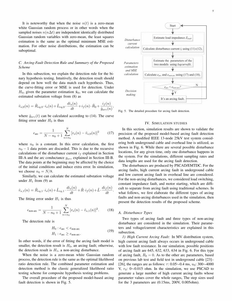
C. Arcing-Fault Detection Rule and Summary of the ProposedScheme

In this subsection, we explain the detection rule for the bi-nary hypothesis testing. Intuitively, the detection result shoulddepend on how well the data match each hypothesis. Thus,the curve-fitting error or MSE is used for detection. UnderH0, given the parameter estimation x0, we can calculate theestimated substation voltage from (8) as

vs,0(n) = Req,0 · is(n)+ Leq,0 ·dis(n)

dt+ if (n) ·R0+

if (n)

garc(n),

where garc(t) can be calculated according to (14). The curvefitting error under H0 is thus

earc =1

N − n0 + 1

N∑n=n0

[vs(n)− vs,0(n)]2 (17)

where n0 is a constant. In this error calculation, the firstn0 − 1 data points are discarded. This is due to the recursivecalculations of the disturbance current if explained in SectionIII-A and the arc conductance garc explained in Section III-B.The data points at the beginning may be affected by the choiceof the initial conditions and induce extra error. In simulation,we choose n0 = N/8.

Similarly, we can calculate the estimated substation voltageunder H1 from (9) as

vs,1(n) = Req,1 ·is(n)+Leq,1 ·dis(n)

dt+R ·if (n)+L· dif (n)

dt.

The fitting error under H1 is thus

enon-arc =1

N − n0 + 1

N∑n=n0

[vs(n)− vs,1(n)]2. (18)

The detection rule is

H0 : earc < enon-arc

H1 : earc ≥ enon-arc.(19)

In other words, if the error of fitting the arcing fault model issmaller, the detection result is H0, an arcing fault; otherwise,the detection result is H1, a non-arcing disturbance.

When the noise is a zero-mean white Gaussian randomprocess, the detection rule is the same as the optimal likelihoodratio detection rule. The combined parameter estimation anddetection method is the classic generalized likelihood ratiotesting scheme for composite hypothesis testing problems.

The overall procedure of the proposed model-based arcingfault detection is shown in Fig. 5.

Start

Estimate load impedance Zload.

Estimate the parameters of the

two models using lsqcurvefit.

Calculate earc and enon-arc using (17) and (18).

Parameters

estimation

and MSE

calculation

Decision

making

Calculate disturbance current if using (11)-(12).

earc < enon-arc?

It’s an arcing fault.

N

Y

Disturbance

current

calculation

Fig. 5. The detailed procedure for arcing fault detection.

IV. SIMULATION STUDIES

In this section, simulation results are shown to validate theprecision of the proposed model-based arcing fault detectionmethod. A modified IEEE 13-node 25kV test system consid-ering both underground cable and overhead line is utilized, asshown in Fig. 6. While there are several possible disturbancelocations, for any given time, only one disturbance happens inthe system. For the simulations, different sampling rates anddata lengths are used for the arcing fault detection.

The disturbances are produced by PSCAD/EMTDC. For thearcing faults, high current arcing fault in underground cableand low current arcing fault in overhead line are considered.For the non-arcing disturbances, we considered load switching,constant impedance fault, and motor starting, which are diffi-cult to separate from arcing fault using traditional schemes. Inwhat follows, we first elaborate the different types of arcingfaults and non-arcing disturbances used in the simulation, thenpresent the detection results of the proposed scheme.

A. Disturbance Types

Two types of arcing fault and three types of non-arcingdisturbance are considered in the simulation. Their parame-ters and voltage/current characteristics are explained in thissubsection.

1) High Current Arcing Fault: In MV distribution system,high current arcing fault always occurs in underground cablewith low fault resistance. In our simulation, possible positionsof arcing fault are 645, 632, 633, 634 in Fig. 6. For this typeof arcing fault, R0 = 0. As to the other arc parameters, basedon previous lab test and field test in underground cable [23]–[26], the ranges are as follows: τ : 0.05∼0.4 ms, u0: 300∼4000V, r0: 0∼0.015 ohm. In the simulation, we use PSCAD togenerate a large number of high current arcing faults whoseparameter values cover the whole ranges, The step sizes usedfor the 3 parameters are (0.15ms, 200V, 0.005ohm).

6

650

632 633 634645

675692

680652

684611 671

Fault location

1.3 km

2.6 km 7.6 km3.2 km

5.3 km4.2 km7.2 km

9.1 km4.2 km

3.3 km

4.1 km646

5.6 km

M

MMotor

starting location

MM

M

Load switching

location

Voltage and currentmeasurement

25kV BUS

Underground

cableOverhead line

Fig. 6. Modified IEEE-13 node test feeder.

50 100 150 200-2

0

2

x 104

t(ms)

Voltage(V)

(a)

50 100 150 200-2

0

2

4x 10

4

t(ms)

Voltage(V)

(b)

tfault

Fig. 7. Voltage waveforms of a high current arcing fault. (a) The bus voltage(vs). (b) Fault point voltage (vf )

The voltage waveforms of the substation voltage vs and faultbranch voltage vf are shown in Fig. 7 for a high current arcingfault where the fault distance is 6 km and the arc parametersare (τ, u0, r0) = (0.0002, 2900, 0.001). The distortion on vf isobvious and the signature square wave shape of an arcing faultcan be clearly seen. However, the substation voltage vs looksvery close to sinusoidal and does not show obvious distortioncompared with vf .

2) Low Current Arcing Fault: The low current arcing faultalways occurs in overhead line with the fault current between15∼100A. In our simulations, possible fault locations are 652,680, and 692 in Fig. 6. For this type of arcing fault, R0 is non-zero, its range is estimated based on phase voltage and faultcurrent range, R0: 100∼900 ohm. Based on [23], the rangesof r0, τ are chosen as τ : 0.05∼0.4 ms, and r0: 0∼0.015 ohm,respectively. As to u0, there is no direct reference on its range.We use the current range for low current arcing fault and therelationship between arc voltage and current introduced in [27]to obtain the following range for u0 as 1000 ∼ 6000 V. In our

50 100 150 200

-200

0

200

t (ms)

Current(A)

(a)

50 100 150 200

-20

0

20

t (ms)

Current(A)

(b)

tfault

Fig. 8. Current waveforms of a low current arcing fault. (a) Feeder currentmeasured at substation (is). (b) Fault current (if )

simulation, a large number of low current arcing faults aregenerated whose parameter values have the following ranges:The step sizes for the four parameters are 200 ohm, 0.15 ms,450 V, and 0.005 ohm, respectively.

In Fig. 8, the waveforms of the substation current is andthe fault current if are presented for a low current arcingfault where the fault distance is 8 km and the arc parametersare (R0, τ, u0, r0) = (700, 0.0002, 2900, 0.004). It can be seenthat the waveform of the simulated low current arcing fault isvery similar to the field test ones in [28].

3) Non-Arcing Disturbances: Three types of non-arcingdisturbance are used in the simulation: load switching, motorstarting and constant impedance fault. These are the faultswith similar features, thus very challenging in discriminatingthem from the arcing fault. The possible locations are shownin Fig. 6. Wide ranges of parameter values of the non-arcing disturbances are used in the simulation. For constantimpedance fault, the fault resistance is between 0.1 and 1500ohm, for motor starting fault, the current ranges from 10A to100 A, for load switching fault, the load current is from 10Ato 80 A.

In Fig. 9, typical current waveforms for the non-arcingdisturbances and arcing faults are compared. It can be seen thatthey have high similarity. The current waveform of constantimpedance fault mimics that of large current arcing fault; andthe current waveform of motor starting and load switching isclose to that of low current arcing fault.

B. Detection Results

In this section, we present the detection results of theproposed model-based scheme. Recall that for given substationvoltage and current measurements, our scheme is to match themeasurements with both the arcing fault model (hypothesisH0) in (8) and the non-arcing disturbance model (hypothesisH1) in (9). The degrees of mismatch or model-fitting MSEare denoted as earc and enon−arc. The detection result is theone with a smaller MSE. Intuitively, larger difference betweenearc and enon−arc means higher detection robustness.

In Fig. 10(a), the MSEs (earc and enon−arc) for high currentarcing faults with different u0 are shown. The parameter u0 ischosen since it is the most sensitive parameter of our proposedscheme. We can see that for all u0 values, earc < enon−arc

7

(a)

(b)

(c)

(d)

(e)

50 100 150 200 250 300

-200

0

200

t(ms)

Current(A)

50 100 150 200 250 300

-200

0

200

t(ms)

Current(A)

50 100 150 200 250 300

-200

0

200

t(ms)

Current(A)

50 100 150 200 250 300

-4000

-2000

0

2000

4000

t(ms)

Current(A)

50 100 150 200 250 300

-4000

-2000

0

2000

4000

t(ms)

Current(A)

Fig. 9. Current waveforms of arcing fault and non-arcing disturbances.(a)High current arcing fault in underground cable. (b) Constant impedance fault.(c) Low current arcing fault in overhead line. (d) Motor starting current. (e)Load switching current.

always. Thus our detection rule in (19) will always producethe correct detection result. The difference of the two MSEsgets larger when u0 increases. Fig. 10(b) is for low currentarcing faults with different R0 values. We can see that for allR0 values, earc < enon−arc always and there is a large gapbetween the two MSE curves.

Results on the non-arcing disturbances are shown in Fig. 11for different parameter values. We can see that for all threetypes of non-arcing disturbance, earc > enon−arc always, thusthe proposed detection scheme always produces the correctdetection result. The gap between the two MSE curves aresignificant, indicating high robustness of the proposed scheme.

Next, we simulate the precision of the proposed detectionscheme via simulation on a large number of faults. The correctdetection probability for different cases are shown in Table Iwhere the sampling rate is 10 kHz so there are 166 points percycle for 60Hz system. The data lengths used for detectionare 0.5, 1, and 2 cycles. We can see that for all disturbancetypes except high current arcing fault, the proposed schemeachieve 100% detection accuracy even when the data lengthis as small as 0.5 cycle. For high current arcing fault, thedetection accuracy is above 98% and increases as the dataused for detection are longer.

In order to verify the robustness of the method, we also

u0 /V(a)

R0 /Ω(b)

100 200 300 400 500 600 700 800 900

2

4

6

8

x 105

Arc model

R-L model

500 1000 1500 2000 2500 3000 3500

1

2

3

4

x 106

VoltageMSE/V2

VoltageMSE/V2

4000

Arc model

R-L model

300 500 700 900

0

1

2

3x 105

Fig. 10. MSE comparison for high current and low current arcing faults. (a)Voltage MSE comparison with different u0 (R0 = 0, τ = 0.0002, r0 =0.004), (b) Voltage MSE comparison with different R0 (τ = 0.0002, u0 =2000, r0 = 0.004).

Load current/ A

VoltageMSE/V2

(a)

(b) Motor starting current/ A

(c) Fault resistance/ Ω

VoltageMSE/V2

VoltageMSE/V2

10 20 30 40 50 60 70

1

2

3x 10

4

10 20 30 40 50 60 70 80 90 100

4

6

8x 10

4

0 500 10001500

1

2

3

4 x 104

80

Arc model

R-L model

Arc model

R-L model

Arc model

R-L model

Fig. 11. MSE comparison for non-arcing disturbances. (a) Voltage MSEcomparison with different load currents (load power factor=0.9). (b) VoltageMSE comparison with different motor starting currents. (c) Voltage MSEcomparison with different fault resistances.

simulate the results for a lower sampling rate at 5 kHz.The results are shown in Table II. We can see that with thelower sampling rate, our scheme still achieves 100% detectionprecision for constant impedance fault, load switching, andmotor starting. For high and low current arcing faults, thedetection probabilities are above 88% and 95%, respectively.As the data lengths grows, the accuracy increases.

V. CONCLUSION

This paper proposes a new model-based detection schemeto discriminate arcing fault from other disturbances in MV dis-tribution systems. We first derive accurate models to representthe behavior of substation voltage for both cases: an arcingfault occurs and a non-arcing disturbance occurs. The voltagedrop on the distribution line is taken into consideration forthe model accuracy. Then the detection problem is formulatedinto a binary hypothesis test. In solving the detection problem,

8

TABLE IRESULTS ON DETECTION ACCURACY (SAMPLING RATE: 10KHZ)

Disturbances Casenumber

Detect rate (%) with dif-ferent data length

0.5 cycle 1 cycle 2 cyclesHigh current arcing fault 960 98.44 98.85 99.06Low current arcing fault 1485 100 100 100Constant impedance fault 532 100 100 100

Load switching 435 100 100 100Motor starting 32 100 100 100

TABLE IIRESULTS ON DETECTION ACCURACY (SAMPLING RATE: 5KHZ)

Disturbances Casenumber

Detect rate (%) with dif-ferent data length

0.5 cycle 1 cycle 2 cyclesHigh current arcing fault 960 88.74 92.49 92.49Low current arcing fault 1485 95.42 96.09 96.9Constant impedance fault 532 100 100 100

Load switching 435 100 100 100Motor starting 32 100 100 100

least-squares parameter estimation and the minimum meansquare-error detection rule are adopted.

The proposed scheme is general in the sense that it candetect both incipient fault in underground cable(high currentarcing fault) and high impedance fault (low current arcingfault), it also can recognize transient fault in overhead line.The method is tested with several different types of arcingfault and non-arcing disturbances, different fault locations, anda large number of disturbance events with different parameters.Simulation results show that the method has high accuracy androbustness when half-cycle or more data are used for detection.

REFERENCES

[1] K. Abdolall, V. L. Buchholz, D. M. Cartlidge, C. P. Morton, G. B.Armanini, A. Harris, and G. F. Valli, “BC Hydro 15 kV cable explosion.”IEEE Trans. Power Delivery, vol. 17, no. 2, pp. 302-307, Apr. 2002.

[2] J. A. Kay and L. Kumpulainen, “Maximizing Protection by MinimizingArcing Times in Medium-Voltage Systems.” IEEE Trans. Industry Appli-cations, vol. 49, no. 4, pp. 1920-1927, Aug. 2013.

[3] M. Sedighizadeh, A. Rezazadeh, and N. I. Elkalashy, “Approaches inHigh Impedance Fault Detection A Chronological Review.” Advances inElectrical and Computer Engineering, vol. 10, no. 3, pp. 114-128, 2010.

[4] C. Benner, K. Butler-Purry, and B. Russell, “Distribution fault anticipa-tor.” EPRI, Palo Alto, CA: 2001. 1001879

[5] S. Kulkarni, S. Santoso, and T. A. Short, “Incipient fault locationalgorithm for underground cables.” IEEE Trans. Smart Grid, vol. 5, no.3, pp. 1165-1174, May 2014.

[6] V. V. Terzija and Z. M. Radojevic, “Numerical algorithm for adaptiveautoreclosure and protection of medium-voltage overhead lines.” IEEETrans. Power Delivery, vol. 19, no. 2, pp. 554-559, Apr. 2004.

[7] T. S. Sidhu and Z. Xu, “Detection of incipient faults in distributionunderground cables.” IEEE Trans. Power Delivery, vol. 25, no. 3, pp.1363-1371, July 2010.

[8] A. D. Stokes and W. T. Oppenlander, “Electric arcs in open air.” Journalof Physics D: Applied Physics, vol. 21, no. 1, pp. 26-35, 1991.

[9] Z. M. Radojevic and J. R. Shin, “New digital algorithm for adaptivereclosing based on the calculation of the faulted phase voltage totalharmonic distortion factor.” IEEE Trans. Power Delivery, vol. 22, no.1, pp. 37-41, Jan. 2007.

[10] Z. M. Radojevic, V. Terzija, G. Preston, and S. Padmanabhan, “Smartoverhead lines autoreclosure algorithm based on detailed fault analysis.”IEEE Trans. Smart Grid, vol. 4, no. 4, pp. 1829-1838, Dec. 2013.

[11] A. Ghaderi, H. A. Mohammadpour, H. L. Ginn, and Y. J. Shin, “High-impedance fault detection in the distribution network using the time-frequency-based algorithm.” IEEE Trans. Power Delivery, vol. 30, no.3, pp. 1260-1268, June 2015.

[12] I. Baqui, I. Zamora, J. Mazon, and G. Buigues, “High impedancefault detection methodology using wavelet transform and artificial neuralnetworks.” Electric Power Systems Research, vol. 81, no. 7, pp. 1325-1333, 2011.

[13] S. Gautam and M. Sukumar, “Detection of high impedance fault inpower distribution systems using mathematical morphology.” IEEE Trans.Power Systems, vol. 28, no. 2, pp. 1226-1234, May 2013.

[14] B. C. Levy, “Principles of signal detection and parameter estimation.”Springer Science & Business Media, 2008.

[15] N. I. Elkalashy, M. Lehtonen, H. A. Darwish, M. A. Izzularab, and A.-K. I. Taalab, “Modeling and experimental verification of high impedancearcing fault in medium voltage networks.” IEEE Trans. Dielectrics andElectrical Insulation, vol. 14, no. 2, pp. 375-383, Apr. 2007.

[16] H. A. Darwish and N. I. Elkalashy, “Universal arc representation usingEMTP.” IEEE Trans. Power Delivery, vol. 20, no. 2, pp. 772-779, Apr.2005.

[17] G. Parise, L. Martirano, and M. Laurini, “Simplified arc-fault model: thereduction factor of the arc current.” IEEE Trans. Industry Application, vol.49, no. 4, pp. 1703-1710, July 2013.

[18] M. Kizilcay and T. Pniok, “Digital simulation of fault arcs in powersystems.” European Trans. on Electrical Power, vol. 1, no. 1, pp. 55-60,Jan. 1991.

[19] G. I. Ospina, D. Cubillos, and L. Ibanez, “Analysis of arcing fault mod-els.” in Proc. 2008 IEEE/PES Transmission and Distribution Conferenceand Exposition: Latin America, pp. 1-5.

[20] M. Michalik, W. Rebizant, M. Lukowicz, and S. J. Lee, “High-impedance fault detection in distribution networks with use of wavelet-based algorithm.” IEEE Trans. Power Delivery, vol. 21, no. 4, pp. 1793-1802, Oct. 2006.

[21] V. Torres, H. F. Ruiz, S. Maximov, and S. Ramirez, “Modeling of highimpedance faults in electric distribution systems.” in Proc. 2014 IEEEInternational Autumn Meeting on Power, Electronics and Computing(ROPEC), pp. 1-6.

[22] S.-J. Lee, M.-S. Choi, S.-H. Kang, B.-G. Jin, D.-S. Lee, N.-S. Yoon,H.-Y. Kim, and S.-B. Wee, “An intelligent and efficient fault location anddiagnosis scheme for radial distribution systems.” IEEE Trans. PowerDelivery, vol. 19, no. 2, pp. 524-532, April 2004.

[23] M. Kizilcay and K. H. Koch, “Numerical fault arc simulation based onpower arc tests.” European Transactions on Electrical Power, vol. 4, no.3, pp. 177-185, May 1994.

[24] B. Koch and P. Christophe, “Arc voltage for arcing faults on 25 (28)-kV cables and splices.” IEEE Trans. Power Delivery, vol. 8, no. 3, pp.779-788, July 1993.

[25] A. Gaudreau and B. Koch, “Evaluation of LV and MV arc parameters.”IEEE Trans. Power Delivery, vol. 23, no. 1, pp. 487-492, Jan. 2008.

[26] S. Kulkarni, A. J. Allen, S. Chopra and S. Santoso, “Waveform charac-teristics of underground cable failures.” in Proc. 2010 IEEE Power andEnergy Society General Meeting, pp. 1-8.

[27] V. V. Terzija and H. J. Koglin, “On the modeling of long arc in still airand arc resistance calculation.” IEEE Trans. Power Delivery, vol. 19, no.3, pp. 1012-1017, July 2004.

[28] J. C. Chen, B. T. Phung, D. M. Zhang, T. Blackburn, and E. Ambikaira-jah, “Study on high impedance fault arcing current characteristics.” in2013 Australasian Universities, Power Engineering Conference (AUPEC),pp. 1-6.

Wenhai Zhang received the B.S. degree in electrical engineering fromSichuan University, Chengdu, China, in 2010. Currently, he is pursuing thePh.D. degree in electrical engineering at Sichuan University, Chengdu, China.Since September 2014, he has been a visiting Ph.D. student with the Universityof Alberta, Edmonton, AB, Canada. His research interests include single-line-to-ground fault detection and location in neutral un-effectively groundedsystem, arcing fault detection and location.