MODEL-BASED DECISION MAKING

IN THE HUMAN BRAIN

Thesis by

Alan Nicolás Hampton

In Partial Fulfillment of the Requirements

for the Degree of

Doctor of Philosophy

CALIFORNIA INSTITUTE OF TECHNOLOGY

Pasadena, California

2007

(Defended May 17th, 2007)

© 2007

Alan Nicolás Hampton

All Rights Reserved

ii

iii

ACKNOWLEDGEMENTS

I would like to thank my thesis advisor and mentor John O’Doherty. I came to his lab with

a passion for science, and an unquenchable curiosity in the most diverse questions about

the functioning of the brain. He not only directed that energy into fruitful endeavors and

provided key insights along the way, but also taught me how to know when enough

research on a given topic had been carried out, how to present the results centered on the

relevant questions, and how to expand the horizon of questions asked given the current

research. In other words, the final sculpting chisels that form a researcher, and lessons

many do not get but through years of experience. Research in John’s lab was not only

productive, it was also eye opening, collegial, and fun.

I also want to thank my collaborator and mentor Peter Bossaerts. With him, John and I

worked on the more complex modeling aspects in this thesis, for which he had a

never-ending stream of insightful advice and groundbreaking ideas. With him I also

explored the implications of risk in human choice, and more generally tied reward-based

decision making with the nascent field of Neuroeconomics. I also want to thank the rest of

my thesis committee: Ralph Adolphs, Shin Shimojo and Steve Quartz for their support,

advice and availability.

During my first two years at Caltech, I worked with Chris Adami and collaborated with

Pietro Perona. Although work carried out during this time is not included in this thesis, the

questions on Bayesian unsupervised learning I explored then have had a direct and

unquestionable impact in my research. I am most grateful to Chris for letting me follow my

ideas to the very end. Without his support, this thesis would not have come to be.

iv

More generally, I want to thank people that, although I did not collaborate directly with,

formed the positive research environment for work in reward based decision making that

forms the backdrop of the Caltech Brain Imaging Center. Thanks Antonio Rangel and

Colin Camerer from HSS, for always being open to questions from people out of their labs,

and Mike Tyszka, Michael Spezio for advice. Thanks Vivian Valentin, Saori Tanaka, Signe

Bray, Hackjin Kim, Elizabeth Tricomi and Klaus Wunderlich in John’s lab; Kerstin

Preuschoff, Tony Bruguier, Ulrik Beierholm, Jan Glaescher, Dirk Neumann, Asha Iyer,

Axel Lindner, Igor Kagan, Hillary Glidden, Hilke Plassmann, Nao Tsuchiya, Jessica

Edwards, Meghana Bhatt, Cedric Anen for fruitful discussions, code sharing, insights and

friendship. Also thanks to Steve Flaherty, Mary Martin and Ralph Lee for making the

CBIC work on wheels.

I also have many friends at Caltech who have made these PhD years pass by with a colorful

tone and who, unbeknownst to them, contributed indirectly to this work by answering

questions relevant to their particular expertise, providing support, interesting side

discussions and creating a fruitful venue to relax. Thanks Grant Mulliken, Allan

Drummond, Kai Shen, and David Soloveichik, with whom I started the CNS program at

Caltech; Alex Holub, Fady Hajjar, Guillaume Brès, Lisa Goggin, Hannes Helgason,

Stephane Lintner, Angel Angulo, Daven Henze, Elena Hartoonian, Corinne Ladous,

Setthivoine You, Alex Gagnon, Jesse Bloom, Vala Hjörleifsdóttir, and Michael Campos. I

also want to thank friends outside of Caltech, who contributed to this work in pretty much

the same way.

Last of all, I want to thank my parents and sisters for the support and patience they have

given during the years. Much of what I am now I owe to them. And to my dearest Allison,

for her love and patience, and for knowing how to encourage me when things got tough,

and tone me down when I was too excited!

v

ABSTRACT

Many real-life decision making problems incorporate higher-order structure, involving

interdependencies between different stimuli, actions, and subsequent rewards. It is not

known whether brain regions implicated in decision making, such as ventromedial

prefrontal cortex, employ a stored model of the task structure to guide choice (model-based

decision making) or merely learn action or state values without assuming higher-order

structure, as in standard reinforcement learning. To discriminate between these possibilities

we scanned human subjects with fMRI while they performed two different decision making

tasks with higher-order structure: probabilistic reversal learning, in which subjects had to

infer which of two choices was the more rewarding and then flexibly switch their choice

when contingencies changed; and the inspection game, in which subjects had to

successfully compete against an intelligent adversary by mentalizing the opponent’s state

of mind in order to anticipate the opponent’s behavior in future. For both tasks we found

that neural activity in a key decision making region: ventromedial prefrontal cortex, was

more consistent with computational models that exploit higher-order structure, than with

simple reinforcement learning. Moreover, in the social interaction game, subjects were

found to employ a sophisticated strategy whereby they used knowledge of how their

actions would influence the actions of their opponent to guide their choices. Specific

computational signals required for the implementation of such a strategy were present in

medial prefrontal cortex and superior temporal sulcus, providing insight into the basic

computations underlying competitive strategic interactions. These results suggest that brain

regions such as ventromedial prefrontal cortex employ an abstract model of task structure

to guide behavioral choice, computations that may underlie the human capacity for

complex social interactions and abstract strategizing.

vi

TABLE OF CONTENTS

Acknowledgements ............................................................................................iii

Abstract ................................................................................................................ v

Table of Contents................................................................................................vi

List of Illustrations.............................................................................................vii

List of Tables ...................................................................................................... ix

Nomenclature....................................................................................................... x

Chapter 1: Introduction ....................................................................................... 1

Chapter 2: Model-based Decision Making in Humans.................................... 12

Chapter 3: Predicting Behavioral Decisions with fMRI.................................. 52

Chapter 4: Amygdala Contributions................................................................. 95

Chapter 5: Thinking of You Thinking of Me................................................. 134

References........................................................................................................ 160

Appendix A: Bayesian Inference ..................................................................... 175

Appendix B: Inference Dynamical Equivalents .............................................. 185

vii

LIST OF ILLUSTRATIONS

Number Page

2.1. Reversal task setup and state-based decision model .................................................31

2.2. Correct choice prior, and posterior - prior update signals in the brain ......................33

2.3. Standard RL and abstract state-based decision models make qualitatively

different predictions about the brain activity after subjects switch their choice. ......35

2.4. Incorrect choice prior and switch - stay signals in the brain ......................................37

S2.1. Comparison of the behavioral fits of the state-based decision model to a

variety of standard Reinforcement Learning algorithms ...........................................44

S2.2. Behavioral data and model predictions for three randomly chosen subjects.............46

S2.3. Plot of the model-predicted choice probabilities derived from the best-fitting

RL algorithm before and after subjects switch their choice. .....................................48

3.1. Reversal task setup and multivariate classifier construction......................................68

3.2. Global and local fMRI signals related to behavioral choice ......................................71

3.3. Illustration of the decoding accuracy for subjects’ subsequent behavioral

choices for each individual region and combination across regions..........................73

S3.1. Brain regions of interest ..............................................................................................77

S3.2. Comparison of fMRI classifiers ..................................................................................79

S3.3. Switch vs. stay for individual subjects........................................................................81

S3.4. Normalized cross-correlation of regression residuals across regions ........................83

S3.5. Classification Receiver Operating Characteristic Curve............................................85

S3.6. Behavioral choice responses and the signal-to-noise ratio in each region of

interest..........................................................................................................................87

S3.7. Regional classifiers......................................................................................................89

viii

4.1. Axial T1-weighted structural MR images from the two amygdala lesion

subjects.......................................................................................................................114

4.2. Probabilistic reversal task..........................................................................................116

4.3. Behavioral performance ............................................................................................118

4.4. Behavioral choice signals..........................................................................................120

4.5. Expected reward signals in the brain ........................................................................122

4.6. Responses to receipt of rewarding and punishing outcomes ...................................124

S4.1. Subject performance during task acquisition............................................................126

S4.2. Controlling for the effects of behavioral differences between amygdala

subjects and controls on signals pertaining to expected reward value.....................128

S4.3. Controlling for behavioral differences between amygdala lesion subjects and

controls in signals pertaining to behavioral choice ..................................................130

S4.4. Multiple axial slices for both amygdala lesion subjects...........................................132

5.1. Inspection game and behavioral results ....................................................................141

5.2. Expected reward signals............................................................................................143

5.3. Influence signals in the brain ....................................................................................145

S5.1. Out-of-sample model log likelihood.........................................................................154

S5.2. Model comparisons with respect to the processing of expected reward signals

in the brain .................................................................................................................156

S5.3. Prediction error signals..............................................................................................158

A.1. Conditional probability distributions of y given a fixed value of the random

variable x ...................................................................................................................176

A.2. Directed graphical model linking six random variables...........................................180

ix

LIST OF TABLES

Number Page

S2.1. Mean parameters across subjects for the behavioral models .....................................50

S2.2. fMRI activity localization ...........................................................................................51

S3.1. Multivariate classifier accuracy in decoding choice across subjects and subject

sessions ........................................................................................................................91

S3.2. Multivariate classifier ROC areas across subjects and subject sessions....................92

S3.3. Regions of interest .......................................................................................................93

5.1. Model update rules ....................................................................................................147

x

NOMENCLATURE

ACC – Anterior Cingulate Cortex

BOLD signal – Blood Oxygenation Level Dependent signal

DLPFC – Dorso-Lateral Prefrontal Cortex

fMRI – Functional Magnetic Resonance Imaging

HMM – Hidden Markov Model

PFC – Prefrontal Cortex

STS – Superior Temporal Sulcus

OFC – Orbitofrontal Cortex

1

C h a p t e r 1

INTRODUCTION

PRELUDE

From an evolutionary perspective, rewards and punishments could be considered as events

that heighten or lower the probability of an organism reproducing. The identification of

what constitutes a rewarding and punishing event for a particular organism can be

considered to be genetically hardwiredi, given that the evaluation of the final objective of

reproductive efficiency is accomplished across various organism generations. These

constitute primary rewards such as food and sex, and primary punishments such as physical

pain; all leading directly or indirectly to heightening or lowering an organism’s survival

and reproduction. Moreover, during the life of an organism, events that are associated to

these primary rewards and punishments can be learnt.

The first organism in which associative learning (classical conditioning) was extensively

studied was with Aplysia’s (a sea hare, shell-less mollusk) siphon-withdrawal reflex. One

defense mechanism that the organism evolved is to withdraw its siphon when it is

stimulated. Stimulation of the tail has no such effect on the siphon. However, after repeated

stimulation of the tail followed shortly by stimulation of the siphon, tail stimulation would

eventually induce siphon withdrawal on its own1, 2. The mechanism by which neurons learn

to associate coincident events was first postulated by Donald Hebb3, and basically states

that the more frequently a pre-synaptic neuron fires coincidently with the firing of a post-

synaptic neuron, the higher the probability that the pre-synaptic neuron will lead to the

firing of the post-synaptic neuron. This type of learning involves a modification of the

i With higher level organisms that have social customs that can be passed on from generation to generation, a second form of evolution

takes place, with the survival of customs that indirectly lead to the survival and reproduction of the organisms that embrace them. Thus, social rewards and punishments are not genetically hardwired, but learnt during the lifetime of an organism, and delivered by the rest of society.

2

synaptic weight, or connectivity, between two neurons through a series of biochemical

reactions at the synaptic site4, 5.

Higher cognitive skills6 basically extend this ability of associating complex external stimuli

with primary rewards and punishments. For example, the visual system can distinguish a

snake from a log (recognition–ventral stream), and understand the movement of objects

(dorsal stream) that lead to upcoming rewarding or punishing events, all from the pattern of

environment light hitting the retina. Furthermore, organisms have a great degree of

freedom in making choices, and many times have multiple, competing predicted rewards

and punishments that could be a consequence of a decision. Thus, the association of

external stimuli with primary rewarding and punishing events has to be condensed into a

final abstract internal value (or utility) to guide decisions. It is from here I will start my

introduction, going quickly over the literature on how organisms might computationally

assign an abstract value (or reward expectation) so as to guide choice in complex, real-

world environments, and start to tease apart the brain structures that execute different

components of these algorithms in the human brain.

STATES AND DECISIONS

The problem to be solved by an organism is to make decisions so as to maximize the

reward, or utility, it obtains. This problem can be broken down into separate components

which will be addressed shortly. Before we do so, I will present a common framework, or

paradigm, to better understand the problem itself. A mechanical view of the world is one in

which the whole environment (including the organism itself in the environment) can be

characterized as a uniquely identifiable state at any point in time, and that the flow of time

is simply having the world jump (transition) from state to state. Having the ability to make

a decision implies that this state flow can be influenced such that the environment (plus

organism) ends up in a given state contingent on the decision made. A simple example is

when a person is in front of two doors. The state he/she is in can be titled ‘in front of two

doors,’ and depending on what door he/she chooses, the ‘left’ or ‘right’ door, he/she will

end in one of two alternative states, i.e., ‘rooms.’

3

The problem of making decisions so as to maximize rewards can be broken down into:

1. State categorization: what makes one state different from another

2. State identification: which state an organism is in

3. State value: the reward/punishment an organism receives as a consequence of being

in a given state

4. State flow: how states change (transition) with time

5. Decisions: how a decision affects the flow of states

Although the world may consist of uniquely identifiable states, an organism still has to

learn and categorize them, leading to an internal representation of world states. This will

not be directly addressed by work in this thesis. The best illustration of the more

biologically oriented advances in the field can be found in research on how the visual

system learns to categorize (and subsequently identify) objects and scenes7, 8 using

unsupervised learning objectives such as sparse9 and predictive coding10. Once an internal

representation of state categories exists, an organism has to infer in what state it is currently

in. Most reward learning research will assume that a state can be perfectly identified,

whereas in real world scenarios an organism will have some uncertainty of which state it is

in, leading to a probability distribution over states. This is the situation when things are

hard to recognize due to environmental noise (Is it a snake or a log?), or when internal

states are not well mapped to environmental states (representation noise). One objective of

learning is to minimize the latter, and make the mapping as good as possible.

Moreover, there is a constraint on the number of states that can be encoded by a brain with

limited capacity. A person from the tropics might define a certain state of water found in

colder regions as ‘solid water,’ while a person from a more temperate region will

differentiate between ‘snow’ and ‘ice.’ This can be defined as a coding problem11. For an

organism, states that happen more often in an environment, or that have a bigger variance

in received rewards and punishments, are better differentiated in comparison to states that

4

do not happen often, or have very similar consequent rewards, which are lumped together

and identified as one single state. Thus, learning how to encode environment states and the

value of those states go hand in hand. Furthermore, it is also advantageous not to encode

the whole environment as one single state (grandmother representation), but as best as

possible as a combination of unique states that can happen independently at the same time

(sparse representation). This is illustrated again with the visual system, in which one can

see more than one object which might have different identities and assigned values, but that

sometimes can be found together in the same scene independently from each other.

However, we will assume the state representation of the environment is given a priori, and

follow up with the question of how values are assigned to existing states through

experience.

With the passage of time, environment states follow one another with certain (physical)

rules. Knowing or having an internal model of how states transform into each other is

useful to predict what is to come, and what rewards to expect in future. The probability of

the environment arriving at a given state may well depend on the history of all previous

states that were visited beforehand. However, this can be relaxed somewhat in many

problems such that the probability of jumping to a state only depends on the current state,

and not on other states further back in history (i.e., a Markov process).

Last, and importantly, is the question of how decisions affect this process. An organism

making a decision ceases to be an observer of the state flow of the environment, with the

rewards it might receive in each state, but rather an active actor who can decide which

state(s) will follow. That is, an organism’s decision defines the probability distribution of

states to follow. This choice will be such so as to maximize the rewards received in the

future, consequent on the environment states visited and decisions made thereafter.

Moreover, organisms apply a discount on future rewards, in part due to their uncertainty

(The type of discounting that humans apply to future monetary rewards is an area of

contention in economic fields12, 13.)

5

COMPUTATIONAL REWARD LEARNING

Given an existing state representation of the environment, we will tease apart how rewards

and decision policies (what decision to make at each state) are learned.

State Values

The most straightforward approach to learning state values is by sampling, in which the

value of the state is updated given the reward the organism receives such that the value is

equivalent to the immediate expected reward sS RV = . This is known as the Rescorla-

Wagner rule14, in which the value of state S is updated with a prediction error, SVR −=δ ,

between the expected value of the state SV and the reward received R :

δη+= SS VV , (1.1)

where η is the learning rate.

From the learned state values, the expectation of future rewards of any given state can be

calculated by adding the value of that state and the value of future states visited thereafter

contingent on the actual decision policy (future decisions), and the discount on future

rewards. The expectation of future rewards then guide decision making. However, knowing

a priori all states and decisions that will be made in the future requires a precise model of

state flow (including future decisions made) and tracing all possible future branches is

computationally intensive and time consuming. An alternative, model-free approach is to

sample the future expected reward of each state directly instead of their immediate

expected reward. The future expected reward of a state can be recursively defined (Bellman

equation15) as the immediate expected reward of that state, plus the expected reward of

future states (expectation over future states visited due to the current decision policy)

reduced with a temporal discount:

)1()()( ++= tStStS VRV γ . (1.2)

6

Thus, future expected rewards can be learned directly with a simple update rule,

)()1( tStS VVR −+= +γδ , known as a temporal difference (TD) update16.

Choice selection

A simple way to decide between two future states is by choosing the one with the highest

sampled value. However, if a state has only been sample a few times, the value of the state

might still be unknown, i.e., there is reward uncertainty. The implicit value of reducing

state uncertainty when making decisions is known as the explore-exploit dilemma17. The

resulting choice stochasticity due to reward uncertainty can be approximated by a softmax

distribution across choices18, in which the probability SP of choosing state S is bigger the

higher its value SV , but where the probability of choosing other states is non-zero

(controlled by a noise or exploration parameter β/1 ):

∑=

i

V

V

S i

S

eeP β

β

.

(1.3)

Furthermore, the reward associated with a given state might not be fixed, but rather a

distribution of values. The most simple, perhaps, is for rewards to have a Gaussian

distribution with a certain mean and variance, given a state. Thus, rewards might randomly

be higher or lower than the mean. This is known as reward risk, and it biases how people

make choices19, 20. Humans not only maximize their expected reward when making

decisions, but also take into consideration the riskiness of those rewards. Furthermore,

humans exhibit risk preferences that change according to whether outcomes are perceived

as gains or losses, something that arguably only depends on how those outcomes are

measured relative to an arbitrary frame: an observation known as prospect theory21.

However, the algorithms presented in this introduction can easily be extended to use utility

values that incorporate both the rewards received and their associated risks. The study of

people’s behavior when making monetary decisions is part of the nascent field of

Neuroeconomics22, 23.

7

Bayesian forward models

As mentioned earlier, a model of state transitions can be constructed to estimate future

expected rewards. In effect, this is a model of the environment dynamics, and it can be used

to look forward at all possible outcomes in the future given the current state. If each state is

also assigned a mean expected reward value (for immediate rewards), then this forward-

looking process can be used to calculate the discounted expected value of that state by

integrating over all future alternative paths. Crucially, forward models have two distinct

components in comparison to sampling-based algorithms. First, the model of how

environment states are linked to each other, and their immediate associated rewards, has to

be learnt. Secondly, the current model can be used to guide decisions by inferring the state

an organism is currently in, and estimating in a forward manner the associated expected

rewards. These two steps can alternate with each other in what is usually referred to as EM

(Expectation-Maximization24), where the first refers to the inference step and the latter to

the learning step (see Appendix A). Moreover, the inference step can be simplified into an

expected value update equation similar to 1.1, but where all the state values are updated

simultaneously as shown below:

)( SSS VRVV −+= η

)( ''' SforegoneSS VRVV −+= η ,

(1.4)

where S is the chosen state, and S’ are the un-chosen or foregone states (see Appendix B for

a complete derivation). The relation between the rewards assigned to update each state not

only depends on the outcome but also on the structure, or relation between states, of the

model. These are not as simple as the reward that would have been received had the other

state been chosen. Thus, it is important to point out that, although expected value update

equivalents are intriguing because of their similarity to RL updating, they are just a proxy

for the correct underlying interpretation: that of hidden state inference.

Summary

Decision making involves knowing the future expected rewards of possible states. This can

be done in a forward model search approach, or in a model-free RL expected reward

8

sampling approach. The first is computationally intensive, time consuming, and assumes

knowledge of the state flow of the environment; while the later is ignorant about

environmental state flow, and computationally quick, but reaches optimal behavior slowly

after extensive sampling of the environment. Furthermore, forward models can be quick to

incorporate new rules and thus adapt to a changing environment, while RL models are quite

slow in adapting to changing reward contingencies. An intermediate approach can be used,

in which expected rewards are computed by taking a few steps into the future with a

forward model, but replacing future steps with sample expected rewards. This combines the

flexibility of forward models (in the short term) with the speed of sampling methods (for

expected rewards further in the future). Likewise, both approaches could be implemented

in parallel and used appropriately, depending on the circumstances25.

BRAIN CORRELATES

The question of which of these algorithms is used by the human brain, and specifically,

what brain structures execute different algorithmic components will now be addressed.

Historically, the first structure to be extensively studied in mammalian brains (rats,

monkeys) was the hippocampus, due to its high neural density which made it easy to record

from extra-cellularly. In particular, these neurons were found to quickly associate incoming

signals (among others, leading to the formulation of the Hopfield network26 as a model of

memory storage in the hippocampus), and to display a variety of adaptive behavior

involving connectivity changes at the synaptic level. The hippocampus is thought to be the

location of declarative associative memory formation27, from which its contents are then

also transferred to other neocortical structures28. Patients with bilateral hippocampal lesions

(from surgical ablation as a corrective measure for seizures, or prolonged alcohol abuse)

cannot form new long term memories but find old memories relatively untouched29, 30,

depending on the damage extent. Thus, hippocampus can be thought of as an integral part

in forming high-level state representations, by associating activities from different cortical

regions.

9

Neural signals in different brain regions have been found to guide choice in a variety of

contexts, from discriminating between noisy sensory stimuli31, 32, to choosing between

stimuli depending on taste33-35, physical pain36-42, and monetary rewards43-47. As discussed

previously, a common reward currency (or utility) should be used to guide choice across

these different modes of rewards and punishments. fMRI studies in humans, and

neurophysiologic studies in rats and primates, have shown activity correlating with reward

expectations across all modalities in mOFC48-52, suggesting this area as encoding an

abstract representation of reward for the guidance of choice53, 54. Moreover, there is

evidence that the interaction between amygdala and mOFC is crucial for the generation of

expected reward signals55, 56. Lesions in mOFC extending up the medial PFC wall have led

to specific deficits in choice behavior: learning is unimpaired, but the ability to adapt to

changing contingencies, such as in reversal learning is diminished56-58.

A key component of reinforcement learning algorithms is the formation of prediction

errors, that is, the difference between rewards obtained and those expected. Schultz, Dayan,

and Montague59 showed that the activity of dopamine neurons in substantia nigra encode

reward prediction errors. Furthermore, they showed that this signal displayed the

characteristics of a temporal prediction error in that reward expectations were progressively

transferred to the earliest state that would predict that reward. Substantia nigra dopamine

neurons mainly project to striatum and medial structures in mOFC, mPFC, and ACC.

Imaging studies find BOLD activity to prediction errors in striatal structures60-63, as well as

temporal difference errors62. The finding of neural structures encoding temporal difference

errors in principle advocate the brain as implementing a model-free approach for state

reward representations, in which future expected rewards are directly encoded for every

environment state. However, these findings do not exclude a model-based approach, in

which states would only encode immediate rewards, and how states predict the next state to

come (state flow) is being learnt. This would imply that a model-based reward expectation

would have to be calculated before a prediction error can be generated. In practice, it is

thought that parallel systems might be computing future expected rewards – a fast and

inflexible model-free approach, and a slow and flexible model-based approach located in

10

mPFC64-66. These two systems might compete when predicting expected rewards, with the

system that makes the most reliable predictions having the final word25.

Last of all, studies have started to look at the effects of reward risk and uncertainty in

guiding behavioral choice67-69. It has also been proposed that the brain might be explicitly

encoding reward risk as a separate signal, so as to arrive at optimal economic decisions70.

DISCUSSION

In this thesis I will provide evidence that reward expectations are not computed solely in a

model-free approach, as advocated by reinforcement learning, but that explicit, model-

based encoding of the structure of the task being solved better explains behavioral choices,

as well as reward expectations and prediction errors in the human brain (Chapter 2). I will

then look at how different brain regions interact to reach model-based decisions (Chapter 3)

and use a whole brain approach to predict what a subject’s next decision will be using

single trial fMRI signals. Finally I study how subjects with localized amygdala lesions

impact the generation of expected reward signals for the guidance of behavioral choice

(Chapter 4). A different, albeit more complex, task was then used to corroborate and extend

these results. Subjects participated in a competitive game in which they had to predict the

opponent’s next choice to guide their own actions (Chapter 5). This involved not only

making a model of the opponent, but players had to understand how their own action

influenced the opponent’s behavior.

The tasks used in this thesis to explore model-based decision making in humans

incorporate two facets. The first is that environment states are not explicit, and subjects

have to create an abstract internal representation of states to solve the tasks. Secondly, the

association of reward contingencies with internal states is assumed known (from training

before the task or from explicit instructions), and thus this thesis is not a study of learning,

but a study of abstract model-based state inference to guide decision making. Optimal state

inference can be formulated using Bayesian estimation (Chapter 2), but simpler equivalent

dynamic equations are later derived (Chapter 4 and 5). A general introduction to Bayesian

inference is provided in Appendix A; and the link between Bayesian inference and the

11

equivalent dynamic equations is made explicit in Appendix B. Conclusions for each study

can be found in the associated chapters.

This body of work shows that humans are not guided solely by model-free RL

mechanisms, but that they do incorporate complex knowledge of the task to update the

values of all choices accordingly. We hypothesize that this is done by creating an abstract

model of environment states on which the task is solved, and from which expected values

are then extracted to guide choice – a process known as model-based decision making.

Furthermore, fMRI BOLD signals subsequent to a subject’s choice reliably encode the

expected reward, as calculated from these model-based algorithms in ventromedial PFC.

More generally, this work shows the value of using optimal choice models to explain

behavior, and then using the internal model variables to tease apart neural processes in the

brain.

Many questions on model-based decision making are left unanswered in this thesis. Most

encompassing is the question of how the brain learns the structure of the model, with its

internal abstract states and associated expected reward values, on which it later infers state

activities to guide decision making as shown in this work. This can be broken in two: the

learning and categorization of environment states, and the learning of how each state

predicts the state that will follow with the flow of time. Understanding how these two

processes are learnt, and the role that reward modulation has, will be an exciting task for

further research.

12

C h a p t e r 2

MODEL-BASED DECISION MAKING IN HUMANSii

Many real-life decision making problems incorporate higher-order structure, involving

interdependencies between different stimuli, actions, and subsequent rewards. It is not

known whether brain regions implicated in decision making, such as ventromedial

prefrontal cortex, employ a stored model of the task structure to guide choice (model-based

decision making) or merely learn action or state values without assuming higher-order

structure, as in standard reinforcement learning. To discriminate between these

possibilities we scanned human subjects with fMRI while they performed a simple decision

making task with higher-order structure: probabilistic reversal learning. We found that

neural activity in a key decision making region – ventromedial prefrontal cortex – was

more consistent with a computational model that exploits higher-order structure, than with

simple reinforcement learning. These results suggest that brain regions such as

ventromedial prefrontal cortex employ an abstract model of task structure to guide

behavioral choice, computations that may underlie the human capacity for complex social

interactions and abstract strategizing.

ii Adapted with permission from Alan N. Hampton, Peter Bossaerts, John P. O’Doherty, “The role of the ventromedial

prefrontal cortex in abstract state-based inference during decision making in humans,” J. Neurosci. 26, 8360-8367 (2006). Copyright 2006 Journal of Neuroscience.

13

INTRODUCTION

Adaptive reward-based decision making in an uncertain environment requires the ability to

form predictions of expected future reward associated with particular sets of actions, and

then bias action selection toward those actions leading to greater reward35, 71.

Reinforcement learning models (RL) provide a strong theoretical account for how this

might be implemented in the brain15. However, an important limitation of these models is

that they fail to exploit higher-order structure in a decision problem, such as

interdependencies between different stimuli, actions, and subsequent rewards. Yet, many

real-life decision problems do incorporate such structure53, 72, 73.

To determine whether neural activity in brain areas involved in decision making is

accounted for by a computational decision making algorithm incorporating an abstract

model of task structure or else by simple reinforcement learning (RL), we conducted a

functional Magnetic Resonance Imaging (fMRI) study where subjects performed a simple

decision making problem with higher-order structure: probabilistic reversal learning53, 74, 75

(Fig. 2.1A). The higher-order structure in this task is the anti-correlation between the

reward distributions associated with the two options, and the knowledge that the

contingencies will reverse.

To capture the higher-order structure in the task, we used a Markov model (Fig. 2.1B) that

incorporates an abstract state variable: the “choice state”. The model observes an outcome

(gain; loss) with a probability that depends on the choice state; if the choice state is

“correct” then the outcome is more likely to be high; otherwise the outcome is more likely

to be low. The observations are used to infer whether the choice state is correct or not. The

crucial difference between a simple RL model and the (Markov) model with an abstract,

hidden state, is that in the former only the value of the chosen option is updated, whereas

the valuation of the option that was not chosen does not change (see Methods); while in the

latter, state-based model, both choice expectations change: if stimulus A is chosen and the

probability that the choice state is “correct” is estimated to be, say, 3/4, then the probability

that the other stimulus, B is correct is assumed to be 1/4 (=1-3/4).

14

One region that may be especially involved in encoding higher-order task structure is the

prefrontal cortex (PFC). This region has long been associated with higher-order cognitive

functions, including working memory, planning and decision making64-66. Recent

neurophysiological evidence implicates PFC neurons in encoding abstract rules76, 77. On

these grounds we predicted that parts of human PFC would correlate better with an abstract

state-based decision algorithm than with simple RL. We focused on parts of the PFC

known to play an important role in reward-based decision making, specifically its ventral

and medial aspects65, 74.

15

RESULTS

Behavioral Measures

The decision to switch is implemented on the basis of the posterior probability that the last

choice was incorrect. The higher this probability, the more likely a subject is to switch

(Fig. 2.1C). The state-based model predicts subjects’ actual choice behavior (whether to

switch or not) with an accuracy of 92±2%. On average, subjects made the objectively

correct choice (chose the action associated with the high probability of reward) on 61±2%

of trials, which is close to the performance of the state-based model (using the parameters

estimated from subjects’ behavior), that correctly selected the best available action on 63%

of trials. This is also close to the maximum optimal performance of 64%, as measured by a

model using the actual task parameters.

Prior correct signal in the Brain

The model estimated prior probability that the current choice is correct (prior correct)

informs about the expected reward value of the currently chosen action. The prior correct

signal was found to have a highly statistically significant correlation with neural activity in

medial prefrontal cortex (mPFC), adjacent orbitofrontal cortex (OFC), and the amygdala

bilaterally (Fig. 2.2; the correlation in medial PFC was significant at a corrected level for

multiple comparisons across the whole brain at p<0.05). These findings are consistent with

previous reports of a role for ventromedial PFC and amygdala in encoding expected reward

value55, 78-81. This evidence has, however, generally been interpreted in the context of RL

models.

In order to plot activity in medial PFC against the prior probabilities, we sorted trials into

one of 5 bins to capture different ranges in the prior probabilities and fitted each bin

separately to the fMRI data. This analysis showed a strong linear relation between the

magnitude of the evoked fMRI signal in this region and the prior correct probabilities

(Fig. 2.2C). We also extracted the % signal change time-courses from the same region and

show these in Fig. 2.2D, plotted separately for trials associated with high and low prior

probabilities. The time-courses show an increase in signal at the time of the choice

16

reflected on trials with a high prior correct, and a decrease in signal at the time of the

choice for trials with a low prior correct.

Posterior – prior correct update

The difference between the posterior correct (at the time of the reward outcome) and the

prior correct can be considered an update signal of the prior probabilities once a

reward/punishment is received. This signal was significantly correlated with activity in

ventromedial PFC as well as in other brain areas such as the ventral striatum (Fig. 2.2B).

This update is also reflected in the time-course plots in Fig. 2.2D. Trials with a low prior in

which a reward is obtained show an increase in signal at the time of the outcome, whereas

trials with a high prior in which a punishment is obtained result in a decrease in signal at

outcome. Thus the response at the time of the posterior differs depending on the prior

probabilities and whether the outcome is a reward or punishment, fully consistent with the

notion that this reflects an update of the prior probabilities.

Abstract-state model vs. standard RL: The response profile of neural activity in

human ventromedial prefrontal cortex

The prior correct signal from the state-based model is almost identical to the expected

reward signal from the RL model. Nevertheless, our paradigm permits sharp discrimination

between the two models. The predictions of the two models differ immediately following a

switch in subjects’ action choice. According to both models, a switch of stimulus should be

more likely to occur when the expected value of the current choice is low, which will

happen after receiving monetary losses on previous trials. What distinguishes the two

models is what happens to the expected value of the newly chosen stimulus after subjects

switch. According to simple RL, the expected value of this new choice should also be low,

because that was the value it had when the subject had previously stopped selecting it and

switched choice (usually after receiving monetary losses on that stimulus). As simple RL

only updates the value of the chosen action, the value of the non-chosen action stays low

until the next time that action is selected. However, according to a state-based inference

model, as soon as a subject switches action choice, the expected reward value of the newly

chosen action should be high, because the known structure of the reversal task incorporates

17

the fact that once the value of one action is low, the value of the other is high. Thus, in a

brain region implementing abstract state-based decision making, the prior correct signal

(which reflects expected value) should jump up following reversal, even before an outcome

(and subsequent prediction error) is experienced on that new action. In RL, the value of the

new action will only be updated following an outcome and subsequent prediction error.

This point is illustrated in Fig. 2.3A where the model predicted expected value signals are

plotted for simple RL and for the state-based model, before and after reversal. Changes in

activation in ventromedial PFC upon choice switches correspond to those predicted by the

abstract state-based model: activation decreases after a punishment and if subject does not

switch, but increases upon switching, rejecting the RL model in favor of the model with an

abstract hidden state (see also Fig. S2.3).

To further validate this point, we conducted an fMRI analysis in which we pitted the state-

based model and the best fitting (to behavior) RL algorithm against each other, to test

which of these provides a better fit to neural activity. A direct comparison between the

regression fits for the state-based model and those for RL revealed that the former was a

significantly better fit to the fMRI data in medial PFC at p<0.001 (Fig. 2.3B). While the

peak difference was in medial PFC, the state-based model also fit activity better in medial

OFC at a slightly lower significance threshold (p<0.01). This suggests that abstract state-

based decision making may be especially localized to the ventromedial PFC.

Prior incorrect

We also tested for regions that correlated negatively with the prior correct, that is areas

correlating positively with the prior probability that the current action is incorrect. This

analysis revealed significant effects in other sectors of prefrontal cortex: specifically right

dorsolateral prefrontal cortex (rDLPFC), right anterior insular cortex, and anterior cingulate

cortex (Fig. 2.4A). Fig. 2.4B shows the relation between the BOLD activity and the model

prior incorrect signal in rDLPFC.

18

Behavioral decision to switch

Finally, we tested for regions involved in implementing the behavioral decision itself (to

switch or stay). Enhanced responses were found in anterior cingulate cortex and anterior

insula on switch compared to stay trials (Fig. 2.4C). This figure shows that regions

activated during the decision to switch are in close proximity to those areas that are

significantly correlated with the prior probability that the current choice is incorrect, as

provided by the decision model.

19

DISCUSSION

In this study we set out to determine whether during performance of a simple decision task

with a rudimentary higher-order structure, human subjects engage in state-based decision

making in which knowledge of the underlying structure of the task is used to guide

behavioral decisions, or if, on the contrary, subjects use the individual reward history of

each action to guide their decision making without taking into account higher-order

structure (standard RL). The decision making task we used incorporates a very simple

higher-order structure: the probability that one action is correct (i.e., leading to the most

reward) is inversely correlated with the probability that the other action is incorrect (i.e.,

leading to the least reward). Over time the contingencies switch, and once subjects work

out that the current action is incorrect they should switch their choice of action. We have

captured state-based decision making in formal terms with an elementary Bayesian Hidden

Markov computational model that incorporates the task structure (by encoding the inverse

relation between the actions and featuring a known probability that the action reward

contingencies will reverse). By performing optimal inference on the basis of this known

structure, the model is able to compute the probability that the subject should maintain their

current choice of action or switch their choice of action.

The critical distinction between the state-based inference model and standard RL is what

happens to the expected value of the newly chosen stimulus after subjects switch.

According to standard RL, the expected value of the new choice should be low, because

that was the value it had when the subject had previously stopped selecting it (usually after

receiving monetary losses on that stimulus). By contrast, the state-based algorithm predicts

that the expected value for the newly chosen action should be high, because, unlike

standard RL, it incorporates the knowledge that when one action is low in value the other is

high. By comparing neural activity in the brain before and after a switch of stimulus, we

have been able to show that, consistent with state-based decision making, the expected

value signal in ventromedial prefrontal cortex jumps up even before a reward is delivered

on the newly chosen action. This updating therefore does not occur at the time of outcome

via a standard reward prediction error (as in standard RL). Rather, the updating seems to

20

occur using prior knowledge of the task structure. This suggests that ventromedial

prefrontal cortex participates in state-based inference rather than standard RL.

Our Bayesian Markov model is just one of a family of models which incorporates the

simple abstract structure of the task. Thus, while we show that vmPFC implements state-

based inference, we remain agnostic about the particular computational process by which

this inference is implemented. Furthermore, our findings do not rule out a role for simple

RL in human decision making, but rather open the question of how abstract-state based

inference and simple RL might interact with each other in order to control behavior25. This

also raises the question of whether the dopaminergic system, whose phasic activity has

been traditionally linked with a reward prediction error in simple RL, subserves a similar

function when the expected rewards are derived from an abstract state representation. An

important signal in our state-based model is the posterior correct, which represents an

update of the prior correct probability based on the outcome experienced on a particular

trial. The difference between the posterior and the prior looks like an error signal, similar to

prediction errors in standard RL, except that the updates are based on the abstract states in

the model. We found significant correlations with this update signal (posterior-prior) in

ventral striatum and mPFC, regions that have previously been associated with prediction

error coding in neuroimaging studies60, 62, 63, 82, 83 (Fig. 2.2B). These findings are consistent

with the possibility that ventromedial prefrontal cortex is involved in encoding the abstract

state-space, while standard reinforcement learning is used to learn the values of the abstract

states in the model, an approach known as model-based reinforcement learning15, 84.

The final decision whether to switch or stay, was associated with activity in anterior

cingulate cortex and anterior insula, consistent with previous reports of a role for these

regions in behavioral control74, 75, 85-88. These regions are in close proximity to areas that

were significantly correlated with the prior probability that the current choice was incorrect,

as provided by the decision model. A plausible interpretation of these findings is that

anterior insula and anterior cingulate cortex may actually be involved in using information

about the inferred choice probabilities in order to compute the decision itself.

21

In the present study we provide evidence that neural activity in ventromedial PFC reflects

learning based on abstract states that capture interdependencies. Our results imply that the

simple RL model is not always appropriate in the analysis of learning in the human brain.

The capacity of prefrontal cortex to perform inference on the basis of abstract states shown

here could also underlie the ability of humans to predict the behavior of others in complex

social transactions and economic games, and accounts more generally for the human ability

of abstract strategizing89.

22

MATERIALS AND METHODS

Subjects

Sixteen healthy normal subjects participated in this study (14 right handed; 8 female). The

subjects were pre-assessed to exclude those with a prior history of neurological or

psychiatric illness. All subjects gave informed consent and the study was approved by the

Institute Review Board at Caltech.

Task description

Subjects participated in a simple decision-making task with higher-order structure:

probabilistic reversal learning. On each trial they are simultaneously presented with the

same two arbitrary fractal stimuli objects (left-right spatial position random) and asked to

select one. One stimulus is designated the correct stimulus in that choice of that stimulus

leads to a monetary reward (winning 25 cents) on 70% of occasions, and a monetary loss

(losing 25 cents) 30% of the time. Consequently choice of this “correct” stimulus leads to

accumulating monetary gain. The other stimulus is “incorrect,” in that choice of that

stimulus leads to a reward 40% of the time and a punishment 60% of the time, leading to a

cumulative monetary loss. The specific reward schedules used here are based on those used

in previous studies of probabilistic reversal learning53, 90. After having chosen the correct

stimulus on 4 consecutive occasions, the contingencies reverse with a probability of 0.25

on each successive trial. Once reversal occurs, subjects then need to choose the new correct

stimulus on 4 consecutive occasions before reversal can occur again (with 0.25

probability). Subjects were informed that reversals occurred at random intervals throughout

the experiment but were not informed of the precise details of how reversals were triggered

by the computer (so as to avoid subjects using explicit strategies such as counting the

number of trials to reversal). The subject’s task is to accumulate as much money as

possible, and thus keep track of which stimulus is currently correct and choose it until

reversal occurs. In the scanner, visual input was provided with Restech (Resonance

Technologies, Northridge, CA, USA) goggles, and subjects used a button box to choose a

stimulus. At the same time that the outcome was revealed, the total money won was also

displayed. In addition to the reversal trials we also included null event trials, which were

23

33% of the total number of trials and randomly intermixed with the reversal trials. These

trials consist of the presentation of a fixation cross for 7 secs. Before entering the scanner,

subjects were informed that they would receive what they earned plus an additional $25

dollars. If they sustained a loss overall then that loss would be subtracted from the $25

dollars. On average, subjects accumulated a total of $3.80 (+/- $0.70) during the

experiment.

Pre-scan training

Before scanning, the subjects were trained on three different versions of the task. The first

is a simple version of the reversal task, in which one of the two fractals yields monetary

rewards 100% of the time and the other monetary losses 100% of the time. These then

reverse according to the same criteria as in the imaging experiment proper, where a reversal

is triggered with probability 0.25 after 4 consecutive choices of the correct stimulus. This

training phase is ended after the subject successfully completes 3 sequential reversals. The

second training phase consists of the presentation of two stimuli that deliver probabilistic

rewards and punishments as in the experiment, but in which the contingencies do not

reverse. The training ends after the subject consecutively chooses the “correct” stimulus 10

times in a row. The final training phase consists of the same task parameters as in the actual

imaging experiment (stochastic rewards and punishments, and stochastic reversals, as

described above). This phase ends after the subject successfully completes 2 sequential

reversals. Different fractal stimuli were used in the training session to those used in the

scanner. Subjects were informed that they would not receive remuneration for their

performance during the training session.

Reinforcement learning model

Reinforcement learning (RL) is concerned with learning predictions of the future reward

that will be obtained from being in a particular state of the world or performing a particular

action. Many different varieties of RL algorithms exist. In this study we used a range of

well known RL algorithms to find the one that provided the best fit to subjects’ choice data

(see Fig. S2.1 for the comparison of behavioral fits between algorithms). The best fitting

RL algorithm was then compared against the state-based decision model for the results

24

reported in the study. See the Behavioral Data Analysis section for a description of the

model-fitting procedure.

The best fitting algorithm to subjects’ choice data was a variant of Q-learning91, in which

action values are updated via a simple Rescorla-Wagner (RW) rule14. On a trial t in which

action a is selected, the value of action a is updated via a prediction error δ:

)()()1( ttVtV aa δη+=+ , (2.1)

where η is the learning rate. The prediction error δ(t) is calculated by comparing the actual

reward received r(t) after choosing action a with the expected reward for that action:

)()()( tVtrt a−=δ . (2.2)

When choosing between two different states (a and b), the model compares the expected

values to select which will give it the most reward in the future. The probability of

choosing state A is:

{ }( )αβσ −−= )()( ba VVAP , (2.3)

where ))exp(1/(1)( zz −+=σ is the Luce choice rule18 or logistic sigmoid, α indicates the

indecision point (when it’s equiprobable to make either choice), and β reflects the degree of

stochasticity in making the choice (i.e., the exploration/exploitation parameter).

Abstract state-based model

We constructed a Bayesian Hidden State Markov ModelHMM, see 92 (HMM) that

incorporates the structure of the probabilistic reversal learning task (Fig. 2.1B), and which

can be solved optimally with belief propagation techniques24. Xt represents the abstract

hidden state (correct or incorrect choice) that subjects have to infer at time t. Yt represents

the reward (positive) or punishment (negative) value subjects receive at time t. And St

represents whether subjects switched or stayed between time t-1 and time t. The conditional

probabilities linking the random variables are as follows:

25

⎟⎟⎠

⎞⎜⎜⎝

⎛−

−==− δδ

δδ1

1),/( 1 staySXXP ttt

⎟⎟⎠

⎞⎜⎜⎝

⎛−

−==− δδ

δδ1

1),/( 1 switchSXXP ttt

),()/( iitt NiXYP σμ== .

(2.4)

The first two conditional probabilities describe the transition probabilities of the hidden

state variable from trial to trial. If the subjects stay (make the same choice as in the

previous trial) and their last choice was correct (Xt-1=correct), then their new choice is

incorrect (Xt=incorrect) with probability δ, where delta is the reversal probability

(probability that the contingencies in the task reverse) and which was considered to be

learnt during training. Likewise, if the subjects stay and their last choice was incorrect

(Xt-1=incorrect), then their new choice will be correct with probability δ. On the other

hand, if subjects switch, with their last choice being incorrect, the new choice might still be

incorrect with probability δ. The state transition matrices in equation 2.4 incorporate the

structural relationship between the reversing task contingencies and subjects’ switches. To

complete the model, we include the probability of receiving a reward P(Y/X) given the state

(correct or incorrect choice) the subjects are in. This was modeled as a Gaussian

distribution whose mean is the expected monetary reward each state has. In the present

task, the actual expected value of the correct choice is 10 cents and the expected value of

the incorrect choice is -5 cents. However, to allow for possible variation in the accuracy of

subjects’ estimates of the expected values of each choice, we left these expected values as

free parameters when fitting the Bayesian model to each subject’s behavioral data. Fitted

parameters for the reversal probability and expected rewards were close to the actual

experimental parameters (Table S2.1).

With P(X0)=(0.5,0.5) at the beginning of the experiment, Bayesian inference was carried

out to calculate the posterior probability of the random variable X (correct/incorrect choice)

given the obtained rewards and punishments (variable Y) and the subjects’ switches

26

(variable S) using causal belief propagation (equations 2.5-2.6). Equation 2.5 specifies the

subjects’ prior, or belief that they will be at a given internal state at time t as a consequence

of their choice St and the internal state posterior from the previous trial. Equation 2.6

updates this prior with the observed reward/punishment Yt to obtain the current posterior, or

optimal assessment of the state at time t. These equations have the Markov property that

knowledge of only the posterior from the previous trial, as well as the last

reward/punishment and behavioral action are needed to calculate the posterior of the next

trial. An introduction to HMMs is provided in the supplementary methods section at the

end of this chapter, as well as in Appendix A.

∑

∑==

==

===−

−−

statesXttt

tttt

statesXttttt

t

t

XXYPcorrectXcorrectXYP

correctX

XSXcorrectXPcorrectX

)()/()()/(

)(

)(),/()(1

11

PriorPrior

Posterior

PosteriorPrior

(2.5)

(2.6)

For the reversal task, the consequence of action switch (or stay) is linear with the inferred

posterior probability that the subjects are making the incorrect (or correct) choice (and so

are the expected rewards). The decision to switch is thus based on the probability that the

current choice is incorrect )( incorrectX t =Posterior (the close correspondence between

the model-estimated posterior that the current choice was incorrect and subjects’ actual

choice behavior is illustrated in Fig. 2.1C). We assume a stochastic relation between actual

choice and the probability that the current choice is incorrect, and use the logistic sigmoid

as in equation 2.3:

{ }( )αβσ −= incorrectPswitchP )( . (2.7)

The state-based model we use here assumes that subjects use a fixed probability of reversal

which is uniform on all trials in which the correct stimulus is being chosen. However, in

actuality the probability of reversal is not uniformly distributed over all the trials, because

after subjects switch their choice the reversal probability is set to zero until subjects make

the correct choice on four consecutive occasions. We compared a version of the state-based

27

model which incorporates the full reversal rule (0 probability of reversal until four

consecutive correct choices are made, and a fixed probability thereafter) to that which

incorporates a simple rule based on a single fixed probability. The latter model was found

to provide a marginally better fit (with a log likelihood of -0.29 compared to -0.40 for the

full model) to subjects actual behavioral choices. This justifies use of a state-based model

with this simplified reversal rule in all subsequent analyses.

Behavioral Data Analysis

Both the RL and state-based model decision probabilities P(switch/stay) were fitted against

the behavioral data B(switch/stay). The state-based model calculates the probability of

switching through equation 2.7. The RL model computes the probability of choosing one

stimulus vs. another, but can be converted to a switch/stay probability based on the

subject’s previous selection (i.e., P(switch)=P(choose A) if the subject chose B in the

previous trial, and vice-versa). On average, subjects switched 22±2 times during the

experiment, out of around 104 trials, so we used a maximum log likelihood fitting criteria

that weighed switching and staying conditions equally:

stay

staystay

switch

switchswitch

NPB

NPB

L ∑∑ +=loglog

log . (2.8)

Model parameters were fitted using a variant of a simulating annealing procedure93. A

comparison of the log likelihoods of the Bayesian model, and a number of RL models is

shown in Fig. S2.1, and a time plot of subject choices vs. model predictions in Fig. S2.2.

The Bayesian model has a better log likelihood fit than the best-fitting RL model (P < 10-7,

paired t-test). This is also true even when using a penalized log likelihood measure (Bayes

Information Criterion – BIC) that takes into account the number of free parameters in each

model94, shown in equation 2.9; where M is the number of free parameters (5 for the

Bayesian model, 3 for the model-free RL) and N the total number of data points.

NNMLBIC loglog2 +−=

(2.9)

28

The mean fitted parameter values across subjects for the Bayesian model and the best-

fitting RL model are shown in Table S2.1. These parameters were used when fitting the

models to the fMRI data. We assumed subjects learned the task structure and reward

contingencies during the training period, and then kept these parameters fixed during task

execution.

We note that while the approach we use here of deriving best-fitting parameters from

subjects’ behavior and then regressing the model with these parameters against the fMRI

data is perhaps the most parsimonious way to constrain our model-based analysis, this

approach assumes that behavior is being controlled by a single unitary learning system with

a single set of model parameters. However, it is possible that behavior may be controlled

by multiple parallel learning systems, each with distinct model parameters83, 95, and, as

such, these multiple learning systems would not be discriminated using our approach.

fMRI data acquisition

Functional imaging was conducted using a Siemens 3.0 Tesla Trio MRI scanner to acquire

gradient echo T2* weighted echo-planar images (EPI). To optimize functional sensitivity in

OFC we acquired the data using an oblique orientation of 30° to the AC-PC line. A total of

580 volumes (19 minutes) were collected during the experiment in an interleaved-

ascending manner. The imaging parameters were: echo time, 30ms; field-of-view, 192mm;

in-plane resolution and slice thickness, 3mm; TR, 2 seconds. High-resolution T1-weighted

structural scans (1x1x1mm) were acquired for anatomical localization. Image analysis was

performed using SPM2 (Wellcome Department of Imaging Neuroscience, Institute of

Neurology, London, UK). Pre-processing included slice timing correction (centered at

TR/2), motion correction, spatial normalization to a standard T2* template with a

resampled voxel size of 3mm, and spatial smoothing using an 8mm gaussian kernel.

Intensity normalization and high-pass temporal filtering (128 secs) were also applied to the

data96.

29

fMRI data analysis

The event-related fMRI data was analyzed by constructing sets of delta (stick) functions at

the time of the choice, and at the time of the outcome. Additional regressors were

constructed by using the model estimated prior probabilities as a modulating parameter at

the time of choice; and the state-based prediction error signal (posterior-prior probabilities)

as a modulating parameter at the time of outcome. In addition, we modeled subjects’

behavioral decision (switch vs. stay) by time-locking a regressor to the expected time of

onset of the next trial (two seconds after the outcome is revealed). All of these regressors

were convolved with a canonical hemodynamic response function (hrf). In addition, the 6

scan-to-scan motion parameters produced during realignment were included to account for

residual motion effects. These were fitted to each subject individually, and the regression

parameters were then taken to the random effects level to obtain the results shown in Figs.

2.2 and 2.4. All reported fMRI statistics and p-values arise from group random effects

analyses. We report those activations as significant in a priori regions of interest that

exceed a threshold of p<0.001 uncorrected, whereas activations outside regions of interest

are reported only if they exceed a threshold of p<0.05 following whole brain correction for

multiple comparisons. Our a priori regions of interest are: prefrontal cortex (ventral and

dorsal aspects), anterior cingulate cortex, anterior insula, amygdala, and striatum (dorsal

and ventral), as these areas have previously been implicated in reversal learning and other

reward-based decision making taskse.g. 74, 82.

Time series of fMRI activity in regions of interest (shown in Fig. 2.2D) were obtained by

extracting the first eigenvariate of the filtered raw time-series (after high-pass filtering and

removal of the effects of residual subject motion) from a 3mm sphere centered at the peak

voxel (from the random effects group level). This was done separately for each individual

subject, binned according to different trial types and averaged across trials and subjects.

SPM normalizes the average fMRI activity to 100, so that the filtered signal is considered

as a percentage change from baseline. It is to be noted that the time-series are not generated

using canonical hrf functions. More specifically, peak BOLD activity is lagged with respect

to the time of the event that generated it. For example, activity arising as a consequence of

30

neural activity at the time of choice will have its maximum effect 4-6 seconds after the time

of choice, as expressed in the time-series plot.

We also compared the best fitting model-free RL and Bayesian algorithms directly

(Fig. 2.3B) by fitting both models at the same time with the fMRI data. To make both

models as similar as possible, we used the normalized value and prediction error signals

from the Rescorla Wagner model as regressors (modulating activity at the time of the trial

onset and outcome respectively), and the normalized prior correct and prediction error

(posterior-prior correct) from the state-based model as regressors (modulating activity at

the time of the trial onset and outcome, respectively). Separate Reward and Punishment

regressors were also fitted at the time of the outcome. Prior correct and value contrasts

were calculated at the individual level and then taken to the random effects level to

determine which areas had a better correlation with the state-based model.

In order to calculate the predicted value and prior correct signals for the standard RL and

state-based model shown in Fig. 2.3, we calculated the expected value (from the RW

model) and prior correct value (derived from the state-based model) on all trials in which

subjects received a punishment and for the immediately subsequent trial. We then sorted

these estimates into two separate categories according to whether subjects switched their

choice of stimulus or maintained their choice of stimulus (stay) on the subsequent trial.

0

0.2

0.4

0.6

0.8

1

0.15 0.25 0.35 0.45 0.55 0.65 0.75 0.85

Stay Switch++

++

++

$2.50$2.50

Trial Onset

A B

~500ms Subject choice

5s Reward delivered

7s Trial ends

X t-1

Yt-1

X t

Y t

S t-1 S t

X 0 X t-1

Yt-1

X t

Y t

S t-1 S t

X 02s choicedisappears

6s Reward disappears++

C

Incorrect choice posterior

0.15 0.25 0.35 0.45 0.55 0.65 0.75 0.850

0.2

0.4

0.6

0.8

1

Ac

tio

n p

rob

ab

ilit

y

Stay Switch

31

32

Figure 2.1. Reversal task setup and state-based decision model. (A) Subjects choose

one of two fractals, which on each trial are randomly placed to the left or right of the

fixation cross. Once a stimulus is selected by the subject it increases in brightness, and

remains on the screen until 2 seconds after the choice. After a further 3s, a reward (winning

25 cents, depicted by a quarter dollar coin) or punishment (losing 25 cents, depicted by a

quarter dollar coin covered by a red cross) is delivered, with the total money earned

displayed at the top. One stimulus is designated the correct stimulus in that choice of that

stimulus leads to a monetary reward on 70% of occasions, and a monetary loss 30% of the

time. Consequently choice of this ‘correct’ stimulus leads to accumulating monetary gain.

The other stimulus is ‘incorrect’, in that choice of that stimulus leads to a reward 40% of

the time and a punishment 60% of the time, leading to a cumulative monetary loss. After

subjects choose the correct stimulus on 4 consecutive occasions, the contingencies reverse

with a probability of 0.25 on each successive trial. Subjects have to infer the reversal took

place and switch their choice, at which point the process is repeated. (B) We constructed an

abstract state-based model that incorporates the structure of the reversal task in the form of

a Bayesian Hidden State Markov Model, which uses previous choice and reward history in

order to infer the probability of being in the correct/incorrect choice state. The choice state

changes (“transits”) from one period to another depending on (i) the exogenously given

chance that the options are reversed (the good action becomes the bad one and v.v.), and

(ii) the control (if subject switches when the actual – but hidden – choice state is “correct”

then the choice state becomes “incorrect” and v.v.). In the diagram, Y is the observed

reward/punishment, S the observed switch/stay action, and X the abstract correct/incorrect

choice state that is inferred at each time step (see Methods). Arrows indicate the causal

relations among random variables. (C) Observed choice frequencies that subjects switch

(black) or stay (grey) against the state-based model’s inferred posterior probability that

their last choice was incorrect. The higher the posterior incorrect probability, the more

likely subjects switch (relative choice frequencies are calculated separately for each

posterior probability bin).

-0.6

-0.5

-0.4

-0.3

-0.2

-0.1

0

0.1

0.2

-3 0 3 6 9 12 15

Time (seconds)

%B

OL

Dre

sp

on

se

High - Pun High - Rew

Low - Pun Low - Rew

-2

-1

0

1

0.3 0.4 0.5 0.6 0.7

Prior correct

Re

gre

ss

ion

co

eff

icie

nt

C D

A Prior correct

L 8

4

0

L

Z = -18Y = +57 X = 0

Ch

oic

e

Fe

ed

ba

ck

L 5

3

1

L

Z = -18Y = + 3 X = - 6

B Posterior - prior

33

34

Figure 2.2. Correct choice prior, and posterior - prior update signals in the brain. (A)

Brain regions showing a significant correlation with the prior correct signal from the state-

based decision model (time-locked to the time of choice). Strong correlations with prior

correct were found in ventromedial prefrontal cortex (mPFC: 6, 57, -6mm; z=5.33 ; OFC:

0, 33, -24mm; z=4.04), as well as in posterior dorsal amygdala (extending into anterior

hippocampus). The activations are shown superimposed on a subject averaged structural

scan and the threshold is set at p<0.001. (B) Brain regions correlating with the posterior-

prior update signal. This is a form of prediction error signal that reflects the difference in

value between the prior probability that the choice will be correct and the posterior

probability that the choice was correct following receipt of the outcome (a reward or

punishment). This signal is significantly correlated with activity in the bilateral ventral

striatum (-24,3,-9mm; z=4.64 and 18,3,-15mm; z=4.48) and medial PFC (-6,54,-24 mm;

z=3.54). These fMRI contrasts are from group random effects analyses. (C) The

relationship between fMRI responses in medial prefrontal cortex (yellow circle in panel a)

at the time of choice and the prior correct signal from the state-based model showed a

strong co-linearity, supporting the idea of an optimal inference of state probabilities. In

order to plot this activity against the prior probabilities, we sorted trials into one of 5 bins to

capture different ranges in the prior probabilities, and fitted each bin separately to the fMRI

data. (D) The time course for the averaged % signal change in this same region (mPFC) is

shown separately for trials with a high prior correct signal (prob. > 0.65) and low prior

correct signal (prob. < 0.5). Error bars depict the standard error of the mean across all trials

of that type. Trials are also separated according to whether a reward or a punishment was

received at the time of outcome to illustrate updating of the signal following feedback. The

leftmost shaded area indicates the period (1 sec in length) in which subjects made their

choice, and the second shaded area the period in which subjects were presented with their

rewarding or punishing feedback. Trials with a low prior in which a reward is obtained

show an increase in signal at the time of the outcome (with the peak BOLD activity lagged

by 4-6 seconds, see Methods), whereas trials with a high prior in which a punishment is

obtained result in a decrease in signal at outcome, consistent with the possibility that the

response at the time of outcome reflects an update signal.

-0.8

-0.4

0

0.4StaySwitch

Punish trial Next trial

Va

lue

Standard RL

0.4

0.5

0.6

Pri

or

co

rre

ct

State-based Model

Punish trial Next trial

-0.2

-0.1

0

0.1

% B

old

re

sp

on

se

mPFC

Punish trial Next trial

+45

L 5

3

1

B State-based > standard RL

A

L

35

36

Figure 2.3. Standard RL and abstract state-based decision models make qualitatively

different predictions about the brain activity after subjects switch their choice. (A)

Both models predict that if a decision is made to stay after being punished, the next action

will have a lower expected value in the next trial (blue line). However, if a decision is made

to switch choice of stimulus after being punished, simple RL predicts that the expected

value of the new choice will also be low (red line – leftmost panel) because its value was

not updated since the last time it was chosen. On the other hand a state-based decision

model predicts that the expected value of the new choice will be high, because if the

subjects have determined that their choice till now was incorrect (prompted by the last

punishment), then their new choice after switching is now correct and has a high expected

value (red line – middle panel). Mean fMRI signal changes (time-locked to the time of

choice) in medial PFC (derived from a 3mm sphere centered at the peak voxel) plotted

before and after reversal (rightmost panel) show that activity in this region is more

consistent with the predictions of state-based decision making than that of standard RL,

indicating that the expected reward signal in mPFC incorporates the structure of the

reversal task. (B) Direct comparison of brain regions correlating with the prior correct

signal from the state-based model compared to the equivalent value signal (of the current

choice) from the simple RL model. A contrast between the models revealed that the state-

based decision model accounts significantly better for neural activity in medial PFC

(shown left panel; 6,45,-9mm; z=3.68).

0.5

1.5

2.5

0.3 0.4 0.5 0.6

Prior Incorrect

Re

gre

ss

ion

co

eff

icie

nt

B

+21 +36

6

4

2

0

A Prior incorrect

L

C Switch - stay

+18 +0

6

4

2

0

L

37

38

Figure 2.4. Incorrect choice prior and switch - stay signals in the brain. (A) Brain

regions showing a significant correlation with the prior incorrect signal from the state-

based algorithm (time-locked to the time of choice). Significant effects were found in right

dorsolateral PFC (39, 36, 33mm; z=4.30), anterior cingulate cortex (6, 21, 45mm; z=3.37),

and right anterior insula (48, 15, 9mm; z=3.96). The threshold is set at p<0.001. (B) Plot

showing relationship between fMRI responses in dorsolateral prefrontal cortex at the time

of choice and the prior incorrect signal from the Bayesian model, illustrating strong co-

linearity between this signal and activity in this region. (C) Brain regions responding on

trials in which subjects decide to switch compared to when they do not switch their choice

of stimulus. Significant effects were found in anterior cingulate cortex (-3, 24, 30mm;

z=4.54) and anterior insula bilaterally (-39, 18, -12mm; z=4.26; 51, 21, 3mm; z=4.23). The

fact that anterior cingulate and anterior insula respond on these switch trials, as well as

responding to the prior incorrect signals, suggests that the decision to switch may be

implemented in these regions.

39

SUPPLEMENTARY METHODS

Reinforcement Learning Models

Q-Learning

These algorithms learn what actions to take when in a given state by learning a value of the

reward that is expected after taking that action. The simplest form, as depicted in the

Methods section in the chapter, updates the value of the action via a simple Rescorla-

Wagner (RW) rule14. On a trial t in which action a is selected, the value of action a is

updated via a prediction error δ:

)()()1( ttVtV aa δη+=+ , (s2.1)

where η is the learning rate. The prediction error δ(t) is calculated by comparing the actual

reward received r(t) after choosing action a with the expected reward for that action:

)()()( tVtrt a−=δ . (s2.2)

Thus, action values reflect the immediate subsequent reward that is expected after taking

that action. This can be extended so as to learn the cumulative rewards expected in the

future, as a consequence of taking a given action. In general, an exponentially discounted

measure of future expected reward is used, in which more weight is given to rewards

expected in the near future in comparison to rewards expected in the far future:

10),()(1

<<= ∑∞

=tt

t rERE γγ (s2.3)

where γ is the discount factor that indicates how near and far future rewards are weighed.

Q-learning can be extended to learn future discounted expected rewards via Temporal

Difference Learning (TD), in which the prediction error used in the value update is:

)()1()()( ' tVtVtrt aa−++= γδ . (s2.4)

40

The effective reward obtained in the next time step due to action a, is a sum of the

immediate reward r(t) and the discounted expected reward due to action a’ in the next time

step. When using Q-learning with temporal difference prediction errors, Q(td), we fitted a

variable number of intermediate states in between the time of choice (t=1) and the time of

reward outcome (t=T), as used in O’Doherty et al.as used in 62. Both Q-learning

algorithms, Q(rw) and Q(td), then stochastically choose the action with most value, as

explained in Methods (equation 2.3).

Actor-Critic

Instead of learning action values directly, as in Q-learning, an alternative approach is to

separate value learning and action selection into two stages97. The first stage, or “Critic,”

involves policy evaluation, in which the expected future rewards that follow from being in

a particular state (corresponding to the average of the expected rewards available for all

selected actions in that state) are learnt. The second stage, or “Actor,” uses the prediction

error signal (δ(t)) derived from the critic to modify of the probability of choosing a given

action so as to increase the average expected reward of the whole policy (equation s2.5).

[ ] )()()1( tPtmtm babaa δδη −+=+

∑=

i

m

m

b i

b

eeP β

β

(s2.5a)

(s2.5b)

The AC(rw) algorithm tested in this chapter uses a Rescorla-Wagner rule (equation s2.2) to

calculate the prediction error δ(t), and the AC(td) algorithm uses Temporal Differences

(equation s2.4) with intermediate state steps between the time of choice and the time of

reward outcome to calculate the prediction error δ(t).

41

Advantage Learning

Advantage Learning is an extension of the actor-critic algorithm98, see also 99. Although

advantage learning differs in a number of respects from actor-critic, the main difference in

terms of the behavioral fitting of the two models in the present case is that in advantage

learning the value of the initial state (time of choice, t=1) is not directly estimated but

instead is set according to:

)2()2()1( =+=== tVPtVPtV bbaa . (s2.6)

BAYESIAN HIDDEN STATE MARKOV MODELS

The key to Bayesian inference is an effective rule, Bayes’ rule, which allows one to infer

the probability of a hidden cause from observable variables.

Imagine a medical situation. A patient visits you repeatedly. Upon visit t, you prescribe her

medication St. The result is a set of symptoms Yt.

In simple reinforcement learning, you learn the relationship between the medication St and

subsequent symptoms Yt. When this patient returns for visit t+1, you use the direct

relationship between both variables which you learnt from all the past pairs of observables

(St,Yt), to determine the choice of medication St+1. Reinforcement learning is flexible

enough to allow for changes in this direct relationship through learning. Effectively,

St

Yt

42

reinforcement learning discounts observable pairs from earlier visits more than from more

recent visits.

Reinforcement learning is only concerned with observables. Bayesian inference, in

contrast, allows for the possibility that there is a hidden cause Xt that determines the

effectiveness of the medication, i.e., the relationship between the medication St and the

symptoms Yt. Bayes’ rule allows one to infer what Xt is given the past observable pairs and

knowledge on how the hidden causes Xt generate the observable symptoms Yt.

To make the example more concrete, one can imagine that Xt takes on 4 values: Xt=0

corresponds to no illness; Xt=1 corresponds to a viral infection; Xt=2 denotes bacterial

infection; Xt=3 stands for allergic reaction. Yt is a measure of nasal symptoms related to

colds, flu and allergic reactions. And St stands for medication (St=0: none; St=1: anti-viral;

St=2: antibiotic; St=3: antihistamine).

Bayesian inference allows one to model explicitly how the “cause” Xt changes over time –

including as a result of the choice variable St (medication, in the case of the example). It is

often assumed that such changes are Markov, which means that the change in X from visit t

to t+1 is influenced only by the immediate past (Xt).

Xt

Yt

St

43

The interpretation of the various components of this Bayesian hidden state Markov model

in the chapter is as follows: St denotes the choice of the subject (St=0 means “stay”; St=1

corresponds to “switch”); Xt denotes the correctness of the choice (Xt=0 means “incorrect

choice”; Xt=1 means “correct choice”); Yt is the observed reward (Yt is a continuous

monetary value, rewards being positive and punishments negative).

Further information on Bayes’ rule, Bayesian inference and Bayesian hidden state Markov

models can be found by D. MacKay100, M. Jordan24, and Z. Ghahramani101.

Xt-1

Yt-1

Xt

Yt

Xt+1

Yt+1

St St+1St-1

A

B

-0.8

-0.7

-0.6

-0.5

-0.4

-0.3

-0.2

State-

based

Q(rw) Q(td) AC(rw) AC(td) Adv.

log

Lik

eli

ho

od

-1.8

-1.6

-1.4

-1.2

-1

-0.8

-0.6

State-

based

Q(rw) Q(td) AC(rw) AC(td) Adv.

ne

ga

tiv

eB

IC

44

45

Figure S2.1. Comparison of the behavioral fits of the state-based decision model to a

variety of standard Reinforcement Learning algorithms, showing that the state-based

model provides a better fit to subjects’ behavioral data than a range of RL

algorithms. The RL algorithms fitted to the subjects’ behavioral data were: Q-learning

Q(rw) using a Rescorla-Wagner update rule, Q-learning Q(td) with intermediate time steps

(assumes multiple time steps within a trial and calculates the expected future reward for

each time step within a trial62, 97), actor-critic AC(rw) with a Rescorla-Wagner update rule,

actor-critic AC(td) with intermediate time steps, and advantage learning (Adv.) – an

extension of the actor-critic algorithm98. (A) The log likelihoods of the action predictions

(switch vs. stay) of each model show that the state-based model provides the best fit to the

data. The second best fitting model is Q-learning using a Rescorla Wagner update rule,

which is the RL algorithm we compared to the state-based model in the fMRI analyses. RL

models are depicted in light blue. (B), The state-based model shows a better fit to the data

even when using the Bayes Information Criterion (BIC) to account for the fact that the

state-based model has more free parameters than the RL models (the number of free

parameters was 5 for the state-based model, 3 for the Q-learning Q(rw) model, 5 for the Q-

learning Q(td) model, 2 for the actor-critic AC(rw), 4 for the actor-critic AC(td), and 4 for

Advantage learning).

0

0.2

0.4

0.6

0.8

1

0 20 40 60 80 100

Sw

itc

hP

rob

ab

ilit

y

0

0.2

0.4

0.6

0.8

1

0 20 40 60 80 100

Sw

itc

hP

rob

ab

ilit

y

0

0.2

0.4

0.6

0.8

1

0 20 40 60 80 100

Sw

itc

hP

rob

ab

ilit

y

0

0.2

0.4

0.6

0.8

1

0 20 40 60 80 100

Sw

itc

hP

rob

ab

ilit

y

0

0.2

0.4

0.6

0.8

1

0 20 40 60 80 100

Sw

itc

hP

rob

ab

ilit

y

0

0.2

0.4

0.6

0.8

1

0 20 40 60 80 100

Sw

itc

hP

rob

ab

ilit

y

46

47

Figure S2.2. Behavioral data and model predictions for three randomly chosen

subjects (subjects 1, 7, 13). The predictions of the state-based decision model (blue line)

as to when to switch correspond more closely to the subjects’ actual switching behavior

(red bar = switch) as compared to the predictions of the best fitting standard RL algorithm

(green line). On top of each graph is the history of received rewards (blue) and punishments

(red), with subjects usually switching after a string of punishments.

0.5

0.6

0.7

0.8

0.9

Ch

oic

eP

rob

Punish Trial Next Trial

48

49

Figure S2.3. Plot of the model-predicted choice probabilities derived from the best-

fitting RL algorithm before and after subjects switch their choice. One possible

alternative explanation for the difference in predictions of the abstract state-based model

and the RL model, is that in the latter we are showing the predictions of value rather than

choice probability. In many RL variants, such as the actor-critic, an anti-correlation

between actions is built in when computing the choice probabilities. Thus, it could be

argued that, had we plotted choice probability from an RL model instead of value, the

predictions of the two models would be much more similar. Here we plot the choice

probability data from the best-fitting RL model, which incorporates a form of anti-

correlation between actions. In spite of this, we still see that the predictions of the choice

probabilities from the RL model do not show the pattern of results we observe for the

abstract-state-based model (where the correct choice probability jumps up following

reversal). This illustrates that a normalized choice probability signal from standard RL does

not emulate the effect predicted by the state-based model, as found to be the case in

ventromedial prefrontal cortex.

50

Table S2.1. Mean parameters across subjects for the behavioral models

Q-learning (Rescorla-Wagner) Learning Rate η α log10 β 0.84 ± 0.03 0.0 ± 0.02 0.6 ± 0.2 State-based decision model Correct mean µC Incorrect mean µI Transition

prob. δ α log10 β

11.3 ± 1.0 cents -7.5 ± 1.3 cents 0.24 ± 0.03 0.55 ± 0.02 1.4 ± 0.2

51

Table S2.2. fMRI activity localization

a) Prior correct activity

brain region laterality x y Z Z-score Ventral medial PFC L/R 6 57 -6 5.33 Posterior amygdala/anterior hippocampus

R 33 -15 -18 4.68

Dorsomedial PFC (frontopolar gyrus) L -9 66 21 4.47 Dorsomedial PFC (frontopolar gyrus) R 6 66 24 4.46 Medial OFC/Subgenual cingulate cortex

L/R 0 39 -6 4.17

Medial OFC L/R 0 33 -24 4.04 Posterior cingulate cortex L/R -9 -57 24 3.98 b) Posterior correct – Prior correct activity

brain region laterality x y z Z-score Medial PFC L -6 54 24 3.54 Ventral striatum L -24 3 -9 4.64 Ventral striatum R 18 3 -15 4.48 c) Prior incorrect activity

brain region laterality x y z Z-score Dorsolateral PFC R 39 36 33 4.30 Anterior insula/frontal operculum R 48 15 9 3.96 Anterior cingulate cortex R 6 21 45 3.37 d) Switch-Stay activity

brain region laterality x y z Z-score Anterior cingulate cortex L/R -3 24 30 4.54 Anterior insula R 51 21 3 4.23 Anterior insula L -39 18 -12 4.26

52

C h a p t e r 3

PREDICTING BEHAVIORAL DECISIONS WITH fMRIiii

While previous studies have implicated a diverse set of brain regions in reward-related

decision making, it is not yet known which of these regions contain information that

directly reflects a decision. Here we measured brain activity using fMRI in a group of

subjects while they performed a simple reward-based decision making task: probabilistic

reversal-learning. We recorded brain activity from 9 distinct regions of interest previously

implicated in decision making, and separated out local spatially distributed signals in each

region from global differences in signal. Using a multivariate analysis approach, we

determined the extent to which global and local signals could be used to decode subjects’

subsequent behavioral choice, based on their brain activity on the preceding trial. We

found that subjects’ decisions could be decoded to a high level of accuracy on the basis of

both local and global signals even before they were required to make a choice, and even

before they knew which physical action would be required. Furthermore, the combined

signals from three specific brain areas: anterior cingulate cortex, medial prefrontal cortex,

and ventral striatum, were found to provide all the information sufficient to decode

subjects’ decisions out of all the regions we studied. These findings implicate a specific

network of regions in encoding information relevant to subsequent behavioral choice.

iii Adapted with permission from Alan N. Hampton, John P. O’Doherty, “Decoding the neural substrates of reward-

related decision making with fMRI,” PNAS (2007). Copyright 2007 Proc. Natl. Acad. Soc. U.S.A.

53

INTRODUCTION

Decision making is a neural process that intervenes between the processing of a stimulus

input and the generation of an appropriate motor output. Motor responses are often

performed in order to obtain reward, and the obligation of a decision making mechanism is

to ensure that appropriate responses are selected in order to maximize available reward.

While the neural systems involved in this process have been the subject of much recent

research, studies have yet to isolate the specific neural circuits responsible for this decision

process. Neural signals have been found that relate to but do not directly reflect this

process, such as those pertaining to the expected value or utility of the available actions35,

73, responses signaling errors in those predictions59, encoding the value of outcomes

received53, as well as responses related to monitoring or evaluation of a previously

executed action87, 102, 103. Such signals have been found in diverse regions throughout the

brain, including, anterior cingulate cortex (ACC), medial prefrontal cortex (mPFC),

orbitofrontal cortex (OFC), dorsolateral prefrontal cortex (DLPFC), amygdala, and

striatum. While complex behavioral decisions are likely to depend on information

computed in a widely distributed network, it is not yet known where among this network of

brain regions neural activity directly reflects the subsequent behavioral decision as to which

action to select.

In order to determine the brain regions where neural activity is directly related to a final

behavioral decision, we applied multivariate decoding techniques to our fMRI data. This

approach combines the temporal and spatial resolution of event-related fMRI with

statistical learning techniques in order to decode on a trial-by-trial basis subjects’ behavior

or subjective states directly from their neural activity. Up to now this technique has been

used in visual perception, to decode perceptual states and/or perceptual decisions from

fMRI signals recorded mainly (though not exclusively) in visual cortical areas104-108. These

previous studies have used locally distributed variations in activity to decode visual

percepts, under situations where the global mean signals in a given region may show no

significant differences between conditions. In the present case, many of our target regions

of interest have been found to show global signal changes related to behavioral choice, that

54

is, large spatially extended cluster areas of activation have previously been reported in

these areas in previous fMRI studies74, 86. Here, in addition to testing for global signals, we

also tested for the presence of locally distributed signals relevant to behavioral decision

making in each of our areas of interest. For this we separated out global and local signals

within each region, and explored the separate contributions of signals at these two different

spatial scales. We then extend this technique to the multi-region level to determine the

contribution of interactions between brain areas in reward-related decision making.

To address this, subjects performed a probabilistic reversal task53, 75 while being scanned

with fMRI. On each trial, subjects are presented with two fractal stimuli and asked to select

one (Fig. 3.1A), with the objective of accumulating as much money as possible. After

making a choice, subjects receive either a monetary gain or a monetary loss. However, one

choice is “correct,” in that choice of that stimulus leads to a greater probability of winning

money and hence to an accumulating monetary gain, while the other choice is “incorrect,”

in that choice of that stimulus leads to a greater probability of losing money and hence to

an accumulating monetary loss. After a time the contingencies reverse so that what was the

correct choice becomes the incorrect choice and vice versa. In order to choose optimally,

subjects need to work out which stimulus is correct, and continue to choose that stimulus

until they determine the contingencies have reversed, in which case they should switch

their choice of stimulus. The goal of our study is to decode subjects’ behavioral choices on

a subsequent trial on the basis of neural activity on the preceding trial.

An important feature of this task is that its probabilistic nature precludes subjects from

inferring which stimulus is correct on the basis of the outcome received on the previous

trial alone, because both correct and incorrect stimulus choices are associated with

rewarding and punishing feedback. Rather, subjects need to take into account the history of

outcomes received in order to make decisions about what choices to make in future.

Furthermore, the two stimuli are presented at random on the left or right of the screen.

Thus, on the previous trial, subjects do not know in advance which of two possible motor

responses are needed to implement a particular decision until such time as the next trial is

triggered. Consequently, our fMRI signal cannot be driven merely by trivial (i.e., non-

55

decision-related) neural activity pertaining to preparation of a specific motor response

(choose left vs. choose right), as such signals are not present before the stimuli are shown.

Therefore, the only signals in the brain relevant to decoding choice are those pertaining to

the subjects’ abstract decision of whether to maintain their current choice of stimulus or

switch their choice to the alternative stimulus, or else the consequences of that decision

(e.g., to implement a switch in behavioral responses).

Nine regions of interest were specified a priori (Fig. S3.1), based on previous literature

implicating these regions in reward-related decision making. These include the medial and

lateral OFC, and adjacent mPFC. These regions have been shown to encode expected

reward values, as well as the reward value of outcomes53, 79, 109. Moreover, signals in these

regions have been found to relate to behavioral choice – whereby activity increases in

medial PFC on trials when subjects maintain their current choices on subsequent trials,

compared to when they switch74

Another region that we hypothesized might contain signals relevant to behavioral choice, is

the ACC. This area is engaged when subjects switch their choice of stimulus on reversal

learning tasks74, 86, suggesting that signals there relate to behavioral choice. A general role

for this region in monitoring action-outcome associations has recently been proposed88.

The region has also been argued to mediate action selection under situations involving

conflict between competing responses87, and action selection between responses with

different reward contingencies46. ACC has also been suggested to play a role in monitoring

errors in behavioral responding, or even in decoding when these errors might occur110.

What all of these accounts of anterior cingulate function have in common is that they posit

an intervening role for this area between the processing of a stimulus input and the

generation of an appropriate behavioral response, even though such accounts differ as to

precisely how this region contributes at this intermediate stage. On these grounds we

hypothesized that neural signals in ACC would be relevant for decoding subsequent

behavioral choices.

56

Other regions we deemed relevant to decision making include the insular cortex, which has

been shown to respond during uncertainty in action choice, as well as under situations

involving risk or ambiguity67, 68, 111. Kuhnen and Knutson69 showed that neural activity in

this region on a previous trial correlated with whether subjects will make a risk-seeking or

risk-averse choice in a risky decision making paradigm. We also include in our regions of

interest ventral striatum, where activity is linked to errors in prediction of future reward,

and dorsal striatum, which is argued to mediate stimulus-response learning as well as goal-

directed action selection62, 82, 112, 113. Another region we included is the amygdala, which has

been implicated in learning of stimulus-reward or stimulus-punisher associations55, 78, 114.

We analyze the contribution each region of interest gives to the decoding of choice

behavior in two ways. In the first, we study each region individually and compare their

discriminative power for decoding behavioral choice. This is done by separating fMRI

signals in each region into spatially local and spatially global signals, thus disambiguating

results that correspond to classic fMRI approaches (global signals), with results that can

only be obtained using multivariate fMRI decoding techniques (local signals). In the

second approach, we make use of neural responses in all of our 9 regions of interest to

decode behavioral decisions by using a multivariate analysis that optimally combines

information from the different brain regions (Fig. 3.1B). This enables us to obtain better

decoding accuracy than by using each region separately, as well as to explore the relative

contributions of each of these different areas to the final behavioral choice.

57

RESULTS

Local vs. global signals related to behavioral choice in regions of interest

To address the contribution of global vs. local signals in the encoding of behavioral choice,

we separated the original fMRI data into global signals with a spatial scale bigger than

8mm, and local signals with a spatial scale smaller than 8mm (see Methods). Fig. 3.2A

shows the statistical significance of each voxel when discriminating between switch vs.

stay decisions in two subjects. Local signals (rightmost images) defined this way do not

survive classical fMRI analysis (Fig. 3.2B), and can only be studied utilizing signal

analysis techniques sensitive to spatially distributed signals. We evaluated the degree to

which each individual region of interest could decode subjects’ subsequent choices, when

using either global or local signals (Fig. 3.3A). Each subject underwent four separate fMRI

sessions (70 trials each) during which they performed the decision making task. Four

classifiers were trained and tested for each subject using four-fold cross validation, where

each classifier is trained using three of the sessions (210 trials), and then tested on the

session that is left out (70 trials). Decoding accuracy derived from global and local signals

were comparable within each region of interest, suggesting that local and global signals

strongly co-vary in each of the regions studied. There was a trend toward a greater

contribution of local signals compared to global signals in overall decoding accuracy in

ACC, although this did not reach statistical significance (at p<0.08)

Decoding accuracy of each individual region

When combining both local and global signals and evaluating decoding accuracy for each

region alone, we find that each region can decode better than chance whether a subject is

going to switch or not (Fig. 3.3B), with the highest accuracies being obtained by ACC

(64%), anterior insula (62%), and DLPFC (60%). To address whether the difference in

decoding accuracy across regions is merely a product of intrinsic differences in MR signal

to noise in these areas, we examined the signal-to-noise ratio (SNR) in each region by

analyzing responses elicited by the main effect of receiving an outcome compared to rest.

All regions had comparable SNR to the main effect (Fig. S3.6), suggesting that accuracy

58

differences are unlikely to be accounted for by variations in intrinsic noise levels between

regions.

Combined accuracy across multiple regions

Next, we aimed to determine whether a combination of specific brain regions would

provide better decoding accuracy than just considering one region alone. For this we built

regional classifiers using a multivariate approach that takes into account interactions

between multiple regions of interest when decoding decisions (see Fig. 3.1B). This

approach optimally combines both local and global signals from each region of interest. In

order to determine which subset of regions to include in our classifier, we performed a

hierarchical analysis whereby we started with the most accurate individual region, and then

iteratively built multi-region classifiers by adding one region at a time. At each step in this

iterative process, we added the region that increased the multi-region classifier’s accuracy

the most (out of the remaining regions). Figure 3.3C shows the results of this process. We

found that out of our nine regions of interest, a classifier with only 3 of these areas – ACC,

mPFC, and ventral striatum – achieved an overall decoding accuracy of 67±2%, a

significantly better decoding accuracy of subject’s choice than that provided by each region

alone (for example, compared to ACC at p<0.01). Accuracy increase when adding regions

is not only due to the signals related to behavioral choice in each region, but also depends

on the degree of statistical independence of noise across regions (Fig. S3.4). Fig. 3.3D

shows the average accuracy for each individual subject when using our region-based

classifier. Receiver Operating Characteristic (ROC) curves representing the average

classifier accuracy across a range of response thresholds are shown in Fig. S3.5 (see also

Table S3.2).

Insula and DLPFC, which on their own have high decoding accuracy, were not selected in

our hierarchical classifier, suggesting that signals from these regions are better accounted

for by the other included regions. To account for the possibility that another combination of

regions could substitute equally well for the regions included in the hierarchical classifier,

we ran an additional analysis whereby we tested the classification accuracy of every

possible combination of three regions (Fig. S3.7). Even in this case we still found that the

59

specific combination of regions identified from the hierarchical analysis were highest in

decoding accuracy compared to all other possible combinations, supporting the conclusion

that the specific regions we identified are sufficient for decoding decisions up to the overall

decoding accuracy obtained in our study.

It should be noted that the approach we use here, whereby signals are combined across

regions, proved significantly better at decoding behavioral decision making than alternative

decoding techniques which do not employ this multi-region approach (Fig. S3.2).

However, when we added more than 4 regions in the hierarchical analysis, the combined

classifier’s accuracy gradually decreased again (Fig. 3.3C), perhaps due to over-fitting of

the training data.

Decisions per se or detection of rewarding vs. punishing outcomes?

A key question is whether the decoding accuracy of our regional classifier is derived by

detecting activity elicited by the decision process and its consequences, or merely reflects

detection of the sensory and affective consequences of receiving a rewarding or punishing

outcome on the preceding trial. To test this, we restricted input to the classifier to only

those trials on which subjects received a punishing outcome. Even in this instance, the

classifier was able to decode subjects’ decisions to switch or stay on the subsequent trial

with 57±1% accuracy, significantly better than chance (at p<10-8, across subjects’ mean

accuracy). This suggests that our classifier is using information relating to the behavioral

decision itself and is not merely discriminating between rewarding or punishing outcomes

on the immediately preceding trial. Additional analyses in support of this conclusion are

detailed in the supplementary material at the end of this chapter.

60

DISCUSSION

The results of this study demonstrate that it is possible to decode with a high degree of

accuracy, reward-related decisions or the consequence of those decisions (in terms of

initiating a change in response choice) in human subjects on the basis of neural activity

measured with fMRI before the specific physical action involved is either planned or

executed. Theoretical accounts of goal-directed behavior differ in the degree to which

decisions are suggested to be linked to the specific action needed to carry them out.

According to one stimulus-driven view, decisions are computed abstractly in terms of the

specific stimulus or goal the subject would like to attain115, 116. In the case of the

probabilistic reversal task used here, this comes down to a choice between which of two

different fractal stimuli to select. An alternative approach is to propose that decisions are

computed by choosing between the set of available physical actions that are required in

order to attain a particular goal. Here, we measure neural responses on a preceding trial

before subjects are presented with the explicit choice between two possible actions, and

before subjects know which specific action they will need to select in order to implement

that decision. The fact that these decisions can be decoded before subjects are aware of the

specific action that needs to be performed to realize them (choose left button or right

button), suggests that decision signals can be encoded in the brain at an abstract level,

independently of the actual physical action with which they are ultimately linked115. We

should note however, that our decoding technique which is based on activity elicited at the

time of receipt of the outcome on the preceding trial, is likely to be picking up both the

decision itself and the consequence of the decision. In other words, once a decision to

switch is computed, a change in stimulus-response mapping is going to be initiated, and the

activity being detected in our analysis may also reflect this additional process.

Our findings have important implications not only for understanding what types of

decisions are computed but also when these decisions are computed. In the context of the

reversal task, it is possible for a decision to be computed at any point in time between

receipt of the outcome on the previous trial, and implementation of the behavioral choice

on the next. By using multivariate fMRI techniques we have been able to show that

61

subsequent decisions (or the consequences of those decisions) can be decoded on the basis

of signals present on the preceding trials (after outcomes are received). This suggests that

the decision to switch or maintain current response set may be initiated as soon as the

information needed to compute the decision is available, rather than being implemented

only when required on the subsequent trial.

In this study we also separated fMRI signals with a global spatial encoding from those with

a local spatial encoding, and evaluated the information each contained for decoding

behavioral choice within each of our regions of interest. Global signals, as we define them

here, are relatively uniform spatially extended clusters of activation within a given area

(with a spatial scale greater than 8mm). Typically, these spatially smoothed signals are

those reported in conventional fMRI analyses, as they are especially likely to survive at the

group level. However, recently it has been shown that information about task processes can

be obtained from considering local spatially distributed variations in voxel activity105, 106. In

the present case, we defined spatially local signals as those with a spatial scale of less than

8mm. In this study we showed that within each region of interest, local signals do convey

important information regarding behavioral choice over and above that conveyed by the

global signals. However, we did not find strong evidence for a dissociation between regions

in the degree to which they were involved in encoding local and global signals, except for a

trend in anterior cingulate cortex toward a greater role for this region in encoding local as

opposed to global signals. These results suggests that at least in the context of the present

reversal learning task, the presence of global and local information relevant to behavioral

decision making strongly covaries within areas. This is in contrast to results observed in the

visual system, where in some instances local signals convey information pertaining to

visual perception even when global signals do not. Local fMRI signals in visual cortex

have been argued to relate to the columnar organization in this area of the brain. It should

be noted however, that much less is known about the degree to which columnar

organization exists outside of visual cortical areas, and hence, the underlying neural

architecture that contributes to local fMRI signals in other areas of the brain such as the

prefrontal cortex remains to be understood.

62

We also used a multivariate analysis technique, whereby the degree to which neural signals

in multiple brain regions contribute to the decision process are evaluated simultaneously.

This approach has allowed us to efficiently recruit signals from diverse brain regions in

order to arrive at a better decoding accuracy for subjects’ behavioral choice than would

follow from considering activity in any one region alone. As a consequence, our findings

suggest that reward-related decision processes might be better understood as a product of

computations performed across a distributed network of brain regions, rather than being the

purview of any one single brain area.

Nevertheless, our results do suggest that some regions are more important than others.

When we compared the decoding accuracy of classifiers incorporating information from all

of our regions of interest to the accuracy of classifiers using information derived from

different subsets of regions, we found that activity in a specific subset of our regions of

interest accounted for the maximum accuracy of our classifier, namely the anterior

cingulate cortex, medial PFC, and ventral striatum. Each of these regions have been

identified previously as playing a role in decision making and behavioral choice on the

basis of prior fMRI studies using traditional statistical analysis techniques74, 82, 86. Out of

these, one region in particular stood out as contributing the most: dorsal anterior cingulate

cortex. This region has been previously implicated in diverse cognitive functions, including

response conflict and error detection87, 110. However, a recent theoretical account has

proposed a more general role for this region in guiding action selection for reward46, 86.

While not incompatible with response-conflict or error-detection theories, our results are

especially consistent with this latter hypothesis, suggesting that this region is playing a key

role in implementing the behavioral decision itself.

Some of the regions featured in this study, such as dorsolateral prefrontal cortex, may

contribute to task or cognitive-set switching more generally117-119 and are unlikely to be

uniquely involved in reward-related decision making. However, it is notable that

dorsolateral prefrontal cortex was ultimately not selected in our combined classifier.

Instead, the regions that were selected have previously been specifically implicated in

63

reward-related learning and/or in implementing changes in behavior as a consequence of

such learning, and not in cognitive set-shifting per se74, 86.

The present study demonstrates that it is possible to decode abstract reward-related

decisions in human subjects on a single trial basis, in essence by reading their decision

before the action is executed. Our findings are consistent with the proposal that decision

making is best thought of as an emergent property of interactions between a distributed

network of brain areas rather than being computed in any one single brain region. Of all the

regions we studied, we found that a subset of three regions seemed to contain information

that was sufficient to decode behavioral decision making: ACC, medial PFC, and ventral

striatum. Future studies are needed to determine whether these regions contain information

specifically required for probabilistic reversal learning or whether other types of reward-

related decisions can also be decoded on the basis of information contained in these areas.

64

MATERIALS AND METHODS

Subjects

Eight healthy, right-handed, normal subjects participated in this study (four female, mean

age 27.6 ± 5.6 SD). The subjects were pre-assessed to exclude those with a prior history of

neurological or psychiatric illness. All subjects gave informed consent and the study was

approved by the Institute Review Board at Caltech. Subjects were paid according to their

performance in the task. Before scanning, subjects were trained on three different versions

of the probabilistic reversal taskas in Chapter 1, 109 (as in Chapter 1), which is also

described in supplementary methods in this chapter.

Data acquisition and preprocessing

The functional imaging was conducted by using a Siemens 3.0 Tesla Trio MRI scanner to

acquire gradient echo T2* weighted echo-planar images (EPI) with BOLD (blood

oxygenation level dependent) contrast. To optimize functional sensitivity in OFC we used a

tilted acquisition in an oblique orientation of 30° to the AC-PC line. Four sessions of 450

volumes each (4x15 minutes) were collected in an interleaved-ascending manner. The

imaging parameters were: echo time, 30ms; field-of-view, 192mm; in-plane resolution and

slice thickness, 3mm; TR, 2 seconds. Whole-brain, high-resolution T1-weighted structural

scans (1x1x1mm) were acquired from each subject and co-registered with their mean EPI.

Image analysis was performed using SPM2 (Wellcome Department of Imaging

Neuroscience, Institute of Neurology, London, UK). To correct for subject motion, the

images were realigned to the first volume, spatially normalized to a standard T2* template

with a re-sampled voxel size of 3mm. Trials were 12 seconds long, and were time locked to

the start of the fMRI EPI scan sequence. This was done to ensure that the scans from the

previous trial used to decode the subject’s decision in the next trial would not be

contaminated with BOLD activity arising from the choice itself on the subsequent trial. A

running high-pass filter (the mean BOLD activity in the last 36 volumes, or 72 seconds,

was subtracted from the activity of the current volume) was also applied to the data. This

was used instead of the usual high-pass filtering96 so that BOLD activity in a volume would

not be contaminated with activity from the choice itself in subsequent volumes. In the

65

scanner, visual input was provided with Restech (Resonance Technologies, Northridge,

CA, USA) goggles, and subjects used a button box to choose a stimulus.

Global and local spatial signals

To dissociate global and local signals relevant to behavioral choice we used the following

procedure: 1) The activity in each voxel was scaled such that the variance of the BOLD

activity over all trials in a session was equalized across all voxels. 2) The fMRI data was

spatially smoothed using a Gaussian kernel with a half width at half maximum (FWHM) of

8mm, to capture global changes in signal. 3) fMRI data containing only locally distributed

spatial signals were then extracted by subtracting the smoothed fMRI data (obtained in step

2) from the non-spatially smoothed fMRI data (obtained in step 1). This procedure adopts

the assumption that BOLD activity is a function of the underlying neuronal activity that is

identical across neighboring voxels, except for a scaling constant. Furthermore, step 1

estimates and eliminates the scaling differences across voxels, but errors in the estimation

of this scaling could lead to an incomplete dissociation between local and global signals.

The procedure also assumes that if local encodings exist, they will have the same spatial

scaling characteristics across all brain regions.

Region of interest (ROI) specification

Nine regions of interest were specified based on previous literature implicating these

regions in reward-related decision making, and delineated by anatomical landmarks (Fig.

S3.1). Regions of interest were specified using a series of spheres centered at specified

(x,y,z) MNI coordinates and with specified radii in millimeters (see Table S3.3 for

complete specification).

Discriminative analysis

To optimally classify whether subjects will switch or stay in a given trial, the fMRI voxel

activity x (see Fig. 3.1A) is assigned to the action ia for which the posterior probability

)()()()|( x|xx papapap iii = is maximal. Here )( iap |x is the distribution of voxel

activities given action ia . Assuming that the fMRI activity x follows a multivariate normal

66

1)(, −=−= Sy Tstayswitch

TT x-xwx w θ

)()()()(

)()(

1211

21

121

)()(

)()|(stay

Tstayswitch

Tswitch

switchT

switch

SS

S

switchestaypeswitchp

eswitchpapxxxxxxxx

xxxx

x−−−−−−

−−−

−−

−

+=

distribution with the same covariance matrix Σ given either action, the posterior

probability whether to choose the switch action is:

(3.1)

where switchx and stayx are the training sample means of the fMRI activity for both actions,

and S is the pooled covariance matrix estimated from the training sample. This can be

simplified to )1(1)|( yswitch eap −+=x , where

(3.2)

Here θ is a threshold variable that groups all constants. Given the brain voxel activity x in

a single trial, choosing the action with maximal posterior is equivalent to choosing the

action for which 0>y .

The classifier was built in two steps (see Fig. 3.1B). In the first, nine regions of interest

were specified (Fig. S3.1), and a unique signal from each region was obtained by adding up

the activities of all voxels in that region, weighted by the voxels’ discriminability:

(3.3)

where 2iσ is the pooled voxel variance of voxel i. This approach assumes that the noise is

independent across voxels, a procedure used to avoid overfitting the classifier to the fMRI

data. The second step utilizes the coalesced regional activities as input to a full Gaussian

discriminative classifier (equation 3.2), where weights are assigned to each region.

Decoding accuracy is measured as the percentage of correctly decoded behavioral choices.

That is, the mean between correctly decoded switch actions (number of correctly decoded

switches divided by the total number of switch actions) and correctly decoded stay actions

2,i

stayi

switchi

iT xxwr

σ-xw ==

67

(number of correctly decoded stays divided by the total number of stay actions). This

measure takes into account the fact that the number of times a subject switches or stays can

be different across sessions.

~.5s Subjectmakes choice

12s Trial ends

3s Reward delivered

2s Fix.

$2.50$2.50

Onset

BOLD response

4s Fixation

Three scans used for decision decoding

within a region between regions

S

MPFCmOFClOFCAmygdalavStriatumdStriatumDLPFCInsulaACCRegion signal Decoding classifer

B Region classifier construction

S

A Trial design

68

69

Figure 3.1. Reversal task setup and classifier construction. (A) Subjects chose one of

two fractals, which on each trial were randomly placed to the left or right of the fixation

cross. The chosen stimulus is illuminated until 2s after the trial onset. After a further 1s, a

reward (winning 25 cents) or punishment (losing 25 cents) is delivered for 1s, with the total

money earned displayed at the top. The screen is then cleared and a central fixation cross is

then presented for 8s before the next trial begins. One stimulus is designated the correct

stimulus in that choice of that stimulus leads to a monetary reward on 70% of occasions,

and a monetary loss 30% of the time. The other stimulus is “incorrect,” in that choice of

that stimulus leads to a reward 40% of the time and a punishment 60% of the time. After

subjects choose the correct stimulus on 4 consecutive occasions, the contingencies reverse

with a probability of 0.25 on each successive trial. Subjects have to infer the reversal took

place and switch their choice, at which point the process is repeated. The last three scans in

a trial are used by our classifier to decode whether subjects will switch their choice or not

in the next trial. A canonical BOLD response elicited at the time of reward receipt is shown

(in green) to illustrate the time-points in the trial at which the hemodynamic response is

sampled for decoding purposes. A new trial was triggered every 12 seconds in order to

ensure adequate separation of hemodynamic signals related to choices on consecutive

trials. The average of three scans between the outcome of reward and the time of choice in

the next trial was used for decoding subjects’ behavioral choice in the next trial. These

three time-points will not only contain activity from the decision itself (activity taking place

after the receipt of feedback, but before the next trial), but also activity from the

reward/punishment received in the current trial, and activity consequent to the choice made

in the current trial. (B) The multivariate region classifier used in this study is divided in two

parts. The first extracts a representative signal from each region of interest (left box) by

averaging the brain voxels within a region weighted by the voxels’ discriminability of the

switch vs. stay conditions. To avoid overfitting the fMRI data, we did not take into

consideration the correlations between voxels within a region of interest (equation 3.3,

Methods). The second part of the classifier (right box) adds up the signal from each region,

weighted by the region’s importance in classifying the subject’s decision (equation 3.2,

Methods). Weights are calculated using a multivariate classifier that uses each region’s

70

decoding strength, and correlations between regions, to maximize the accuracy of the

classifier in decoding whether subjects are going to switch or stay (see Methods –

Discriminative analysis).

A Global vs. Local activity

+

+

Original Global Local

Original Global Local

S1

S2

Original Global Local

+

B Random effects

71

72

Figure 3.2. Global and local fMRI signals related to behavioral choice (A) Here we

show fMRI signals related to behavioral choice, i.e., whether subjects will switch or

maintain (stay) their choices on a subsequent trial. Voxel t-scores for the discriminability

between switch and stay trials is shown for 2 individual subjects with data in its original

form (left-most panel), and then decomposed into a global spatial component (with spatial

scale > 8mm, middle panel) and a local spatial component (spatial scale < 8mm, right

panel). The ACC region of interest is outlined in white for reference. Red and yellow colors

indicate increased responses on switch compared to stay trials, while blue colors indicate

stronger responses on stay compared to switch trials. (B) Results from a group random

effects analysis across subjects conducted separately for the original unsmoothed data,

global data, and local data. While global signals survive at the random effects level

(consistent with classical fMRI analyses), local spatial signals do not survive at the group

random effects level. Random effect t-scores are shown with a threshold set at p<0.2 for

visualization.

+VStri

at.

Accu

racy

AC

um

ula

tive

Acc

ura

cy

C Regional Classifier Ordering

58%

62%

66%

70%

+MPFC

+MO

FC

+Am

yg.

+DStri

at.

+LO

FC

+In

sula

AC

C

+DLP

FC

Global Local B Individual Regionsm

PFC

mO

FC

Am

yg.

vStri

at.

dStri

at.

LOFC

Insu

laAC

C

DLP

FC

Accu

racy

55%

60%

65%

50%

60%

65%

70%

55%

1 2 3 4 5 6 7 8

Subjects

D Individual SubjectsA

ccu

racy

75%

55%

60%

65%

50%

mPFC

mO

FC

Am

yg.

vStri

at.

dStri

at.

LOFC

Insu

laAC

C

DLP

FC

73

74

Figure 3.3. Illustration of the decoding accuracy for subjects’ subsequent behavioral

choices for each individual region and combination across regions (A) Plot of average

accuracies across subjects shown separately for local and global spatial scales. Both spatial

scales contain information that can be used to decode subjects’ subsequent behavioral

choice in all of our regions of interest. Notably, decoding accuracies are comparable at the

local and global scales within each region. (B) Plot of average across accuracy across

subjects for each region individually combining both local and global signals. (C) Results

of the hierarchical multi-region classifier analysis, averaged across subjects. An ordering of

regions was performed by starting with a classifier which only contains the individual

region with best overall accuracy (ACC, left column), and iteratively adding to this

classifier the regions whose inclusion increases the accuracy of the classifier the most (or

decreases the least). Thus, the second column shows the accuracy of a classifier containing

ACC and ventral striatum, the third column the accuracy of a classifier containing ACC,

ventral striatum, and mPFC, and so forth. The combination of the three regions which

provide the best decoding accuracy are highlighted in grey. Addition of a fourth region

(dorsal striatum) does not significantly increase decoding accuracy. All error bars indicate

standard errors of the mean. (D) Decoding accuracy for the three-region classifier shown

separately for each individual subject (Table S3.1).

75

MATERIALS AND METHODS

Pre-scan training

Before scanning, subjects were trained on three different versions of the task. The first is a

simple version of the reversal task, in which one of the two fractals presented yields

monetary rewards 100% of the time and the other monetary losses 100% of the time. These

then reverse according to the same criteria as in the imaging experiment proper, as

described in Fig 3.1A. This training phase is ended after the subject successfully completes

3 sequential reversals. The second training phase consists of the presentation of two stimuli

that deliver probabilistic rewards and punishments as in the experiment, but where the

contingencies do not reverse. The training ends after the subject consecutively chooses the

‘correct’ stimulus 10 times in a row. The final training phase consists of the same task

parameters as in the actual imaging experiment. This phase ends after the subject

successfully completes 2 sequential reversals. Different fractal stimuli were used in the

training session than those used in the scanner. Subjects were informed that they would not

receive remuneration for their performance during the training session.

76

SUPPLEMENTARY ANALYSES

Dissociating the contribution of reward vs. punishment signals on the immediately

preceding trial from behavioral choice signals in the classification analysis

In order to determine whether our decision classifier was using information above and

beyond that pertaining to receipt of rewards and punishers on the previous trial, we first

explored how much information receiving a reward or a punishment on the previous trial

provides about the subsequent behavioral choice. For this, we looked only at subjects’

reward and punishment histories (leaving aside their fMRI data), and trained a classifier to

decode subjects’ subsequent choices on the basis of rewards and punishments received on

an immediately preceding trial. This classifier was able to decode subjects choices with

63±1% accuracy, a decoding accuracy lower than that achieved by the classifier based on

the fMRI data (of 67±2%, p<0.07 paired t-test across subjects). The decoding accuracy of

the naïve classifier was due to the probabilistic nature of the task; in which subjects will

sometimes switch and sometimes stay following receipt of a punishing outcome, but will

always stay after receipt of a reward.

In addition to decoding behavioral decisions from brain activity, we also tested a classifier

in order to determine whether on a given trial subjects received a reward or a punishment.

This classifier (using the same three regions of interest as used for our decision classifier)

was able to decode subjects’ receipt of a reward or punishment with 70±1% accuracy. This

shows that these regions are sensitive not only to the actual behavioral decision, but also to

whether subjects’ received a rewarding or a punishing outcome. Nevertheless, these

findings also confirm that our decision classifier has to be using much more information

than merely reading responses to the rewarding or punishing outcomes received on the

previous trial, as the fact that rewards and punishments themselves can only be decoded up

to an accuracy of 70% suggests that reward and punishment information on the

immediately preceding trial probably constitutes a relatively minor contribution toward the

overall accuracy of the decision classifier (because as shown above, even with 100%

decoding accuracy, rewards and punishments on the previous trial can only decode 63% of

subsequent decisions).

Medial PFC Amygdala Dorso Lateral PFC

Frontal InsulaVentral StriatumMedial OFC

Lateral OFC Dorsal Striatum ACC

77

78

Figure S3.1. Brain regions of interest. Nine regions of interest were specified. These are:

medial PFC, adjacent medial and lateral OFC, amygdala, ventral and dorsal striatum, left

and right DLPFC, anterior insula, and ACC. fMRI signals in each region were used to

decode subjects’ behavioral choices using a two-step multivariate classifier (see Fig. 3.1B).

Table S3.3 specifies the coordinates of these regions of interest.

Acc

ura

cy

Three Regions Combined

Whole Brain

Best Voxels

60%

65%

70%

55%

50%

79

80

Figure S3.2. Comparison of fMRI classifiers. Adding up all the brain voxels weighted by

their discriminability (in decoding stay vs. switch decisions), which assumes voxels are

independent of each other, yielded an accuracy of 61%. When taking the 20 individually

best discriminating voxels and adding them independently, it yielded an accuracy of 64%.

Our multivariate region-based classifier, which combines three regions of interest, yielded

an average accuracy across subjects of 67% (blue column), significantly better than the

other techniques (e.g., at p<0.04, paired t-test when compared to the 20 best voxel

classifier). Error bars are fixed effects across subject sessions.

81

82

Figure S3.3. Switch vs. stay for individual subjects. Results of a simple linear contrast

between signals in regions of interest derived from averaging the last 3 scans in a trial (after

the receipt of outcome), according to whether subjects switch or stay on the subsequent

trial, using smoothed data (global signals). The figures show t-scores within each region of

interest that reflect the difference in signals between trials in which subjects subsequently

switch their choice of stimulus to those trials where subjects stay (or maintain their

previous choice of stimulus). Red and yellow colors indicate increased responses on switch

compared to stay trials, while blue colors indicate stronger responses on stay compared to

switch trials.

0

0.2

0.4

0.6

0.8

1mPFC

mOFC

Amyg.

vStriat.

dStriat.

LOFC

Insula

ACC

DLPFC

Normalized Cross Correlation

mPFC

mO

FC

Am

yg.

vStri

at.

dStri

at.

LOFC

Insu

laAC

C

DLP

FC

83

84

Figure S3.4. Normalized cross-correlation of regression residuals across regions.

Regression residuals correspond to aspects of task processing that are not directly related to

the subject’s behavioral decision; such as preparation of motor responses and stimulus

processing. These processes can be shared between regions, thereby introducing

correlations in time-courses between regions. The normalized cross-correlation matrix plot

shown here illustrates the correlation between regions, after activity related to the decision

has been removed. Each region is plotted on the vertical and horizontal axes, and

correlations between any two regions can be found by finding the square corresponding to

the intersection between the regions on these two axes. The color of each square depicts the

intensity of the correlation, ranging from blue (uncorrelated) to red (fully correlated), see

attached color scale. The diagonal elements express the correlation of the signal of a region

with itself, and are by definition equal to one. The cross-correlation of residuals across

regions shows a strong sharing of task processes between DLPFC, insula, and ACC (lower

right triplet). In addition, ventral and dorsal striatum were found to be highly correlated in

their activity. We also found weak correlations between residual activity in mPFC and

medial OFC, and between DLPFC and OFC. In general, brain regions that are closer to

each other in terms of physical distance, present higher inter-correlations than regions that

are more distal, perhaps reflecting increased coupling between regions as a function of

local connectivity.

0% 25% 50% 75% 100%0%

25%

50%

75%

100%

False Positive Rate

Tru

eP

ositiv

eR

ate

0% 25% 50% 75% 100%0%

25%

50%

75%

100%

False Positive Rate

Tru

eP

ositiv

eR

ate

0% 25% 50% 75% 100%0%

25%

50%

75%

100%

False Positive Rate

Tru

eP

ositiv

eR

ate

0% 25% 50% 75% 100%0%

25%

50%

75%

100%

False Positive Rate

Tru

eP

ositiv

eR

ate

0% 25% 50% 75% 100%0%

25%

50%

75%

100%

False Positive Rate

Tru

eP

ositiv

eR

ate

0% 25% 50% 75% 100%0%

25%

50%

75%

100%

False Positive Rate

Tru

eP

ositiv

eR

ate

0% 25% 50% 75% 100%0%

25%

50%

75%

100%

False Positive Rate

Tru

eP

ositiv

eR

ate

0% 25% 50% 75% 100%

0% 25% 50% 75% 100%0%

25%

50%

75%

100%

False Positive Rate

Tru

eP

ositiv

eR

ate

0% 25% 50% 75% 100%0%

25%

50%

75%

100%

False Positive Rate

Tru

eP

ositiv

eR

ate

0% 25% 50% 75% 100%0%

25%

50%

75%

100%

False Positive Rate

Tru

eP

ositiv

eR

ate

0% 25% 50% 75% 100%0%

25%

50%

75%

100%

False Positive Rate

Tru

eP

ositiv

eR

ate

85

86

Figure S3.5. Classification Receiver Operating Characteristic Curve. A measure used

in signal detection to measure classifier discriminability is the area under a Receiver

Operating Characteristic (ROC) curve120, which represents the average classifier accuracy

across all possible thresholds. Here we show typical ROC curves for the four sessions from

one subject: blue for the session classifier on the training data, and red on the testing data.

An area of 100 means the classifier will have on average an accuracy of 100%, and an area

of 50 means that on average the classifier will have a 50% accuracy. Across subjects, ROC

curves indicated an average accuracy of 71±2% for decoding behavioral choices over all

sessions (Table S3.2). The ROC curves of the classifiers for the training data and testing

data are very similar, indicating that our procedure for training the discriminative classifier

across regions of interest does not over-fit the fMRI data.

0

1

2

3

-2

-1

0

1

2

3

4

0

1

2

3

4

5

6

7

0

1

2

3

0

1

2

3

mPFC

mO

FC

Am

yg.

vStri

at.

dStri

at.

LOFC

Insu

laAC

C

DLP

FC

mPFC

mO

FC

Am

yg.

vStri

at.

dStri

at.

LOFC

Insu

laAC

C

DLP

FC

mPFC

mO

FC

Am

yg.

vStri

at.

dStri

at.

LOFC

Insu

laAC

C

DLP

FC

mPFC

mO

FC

Am

yg.

vStri

at.

dStri

at.

LOFC

Insu

laAC

C

DLP

FC

A - Switch-Stay Classifier

Avg. Normalized Weights Avg. Norm. Weight Power

Avg. Region T-score Avg. Region T-score Power

B - Region Main Effects

87

88

Figure S3.6. Behavioral choice responses and the signal-to-noise ratio in each region

of interest. The fact that we find some regions to have higher decoding accuracy than

others could reflect either a greater contribution of a given region toward computing a

decision (and its consequences), or alternatively could be merely ascribed to global

differences in the signal-to-noise ratio of the fMRI signal between regions. To account for

this, we compared the sensitivityiv of each region to the behavioral choice signals (top-right

panel), with the sensitivity of each region as estimated from responses to the main effect at

the time of outcome (bottom-right panel). As can be seen, SNR is comparable across

regions of interest, and thus differences in behavioral choice sensitivity across regions are

unlikely to be accounted for merely by an overall difference in SNR across these areas. The

left panels show the average classifier normalized discriminant weights (t-scores) across

subjects. Although some regions have classification power (sensitivity), they average out

across individuals because they have different signs across regions.

iv An unsigned mean sensitivity across subjects was obtained by 1) squaring the SNR per subject, 2) transforming to z-scores with an

inverse F distribution 3) averaging z-scores across subjects 4) transforming back with an F distribution 4) taking the square root.

Acc

ura

cy

Combination of 3 regions of interest

0 10 20 30 40 50 60 70 80

56

58

60

62

64

66

68

89

90

Figure S3.7. Regional classifiers. In Fig. 3.3D we created classifiers with an increasing

number of regions to find the minimum set of regions that provided the maximum accuracy

when decoding subjects’ decisions. However, the process might be misleading in that there

might be a different combination of N regions that is better than a classifier with N regions

built hierarchically. To test for this, we computed classifier accuracy for all combinations

of three regions (out of 9). The accuracy of each combination of regions is shown ordered

from left to right with the right most column corresponding to the best combination of

regions (shown in black). This turns out to be ACC, ventral Striatum and mPFC, which

enjoys a 1% advantage in decoding accuracy over the next best combination of regions.

Thus, the results of this analysis accord with the hierarchical analysis in highlighting the

three regions identified from that analysis as providing the most information for decoding

behavioral choice out of all regions tested.

91

SUPPLEMENTARY TABLES

Table S3.1. Multivariate classifier accuracy in decoding choice across subjects and

subject sessions

Subject 1 2 3 4 5 6 7 8 Mean Sess. 1 69% 69% 73% 67% 59% 57% 64% 57% 64±2%Sess. 2 73% 52% 62% 79% 76% 63% 68% 63% 67±3%Sess. 3 61% 83% 81% 76% 81% 55% 61% 60% 70±4%Sess. 4 74% 63% 81% 77% 70% 64% 56% 57% 68±3%Mean 69±3% 67±6% 74±4% 75±3% 72±5% 59±2% 62±3% 59±1% 67±2%

92

Table S3.2. Multivariate classifier ROC areas across subjects and subject sessions

Subject 1 2 3 4 5 6 7 8 MeanSess. 1 74 74 76 68 63 54 66 68 68±3 Sess. 2 83 63 67 82 76 66 74 61 71±3 Sess. 3 65 86 90 82 85 61 65 76 76±4 Sess. 4 76 65 80 77 72 65 63 57 69±3 Mean 74±4 72±5 78±5 77±3 74±5 61±3 67±2 66±4 71±2

93

Table S3.3. Regions of Interest. Each region of interest is specified by a series of

spheres centered at the specified (x, y, z) MNI coordinates and radius (mm).

mPFC x y z radius 0 52 0 12 0 50 11 12 0 47 21 12 0 52 33 12 0 59 23 12 0 64 12 12 0 65 1 12 0 60 -9 12

mOFC x y z Radius 0 38 -26 12 0 40 -26 12 0 42 -26 12 0 44 -26 12 0 46 -26 12 0 48 -26 12

lOFC x y z Radius 25 50 -21 10 26 43 -21 10 26 38 -21 10 -25 50 -21 10 -26 43 -21 10 -26 38 -21 10

Amygdala x y z radius 20 -2 -29 10 -20 -2 -29 10 23 -11 -27 8 -23 -11 -27 8 28 -17 -23 8 -28 -17 -23 8

DLPFC x y z radius -43 23 50 25 -43 46 39 25 -43 63 16 25 43 23 50 25 43 46 39 25 43 63 16 25

Insula x y z radius 36 23 0 10 -36 23 0 10

vStriatum x y z radius -20 15 -9 4 -19 10 -9 5 -22 10 -14 5 -17 10 -16 5 -10 10 -16 5 -14 10 -12 5 -10 5 -16 5 -17 5 -16 5 -19 5 -9 5 -22 5 -4 5 -18 13 -11 5 -15 5 -13 5 20 15 -9 4 19 10 -9 5 22 10 -14 5 17 10 -16 5 10 10 -16 5 14 10 -12 5 10 5 -16 5 17 5 -16 5 19 5 -9 5 22 5 -4 5 18 13 -11 5 15 5 -13 5 3 10 -16 5 -3 10 -16 5 3 5 -16 5 -3 5 -16 5 0 10 -16 5 -5 10 -16 5 5 10 -16 5 0 5 -16 5 -5 5 -16 5 5 5 -16 5

94

dStriatum x y z radius -13 16 8 5 -13 11 13 5 -12 5 15 5 -9 11 8 5 -10 16 3 5 -9 17 -2 5 -10 7 11 5 13 16 8 5 13 11 13 5 12 5 15 5 9 11 8 5 10 16 3 5 9 17 -2 5 10 7 11 5

ACC x y z radius 0 26 29 12 0 18 33 12 0 6 38 12 0 27 40 12 0 17 46 12 0 6 50 12

95

C h a p t e r 4

AMYGDALA CONTRIBUTIONSv

The prefrontal cortex receives substantial anatomical input from the amygdala, and these

two structures have long been implicated in reward-related learning and decision making.

Yet little is known about how these regions interact, especially in humans. We investigated

the contribution of the amygdala to reward-related signals in prefrontal cortex by scanning

two rare subjects with focal bilateral amygdala lesions using fMRI. The subjects performed

a reversal learning task in which they first had to learn which of two choices was the more

rewarding, and then flexibly switch their choice when contingencies changed. Compared to

healthy controls, both amygdala lesion subjects showed a profound change in ventromedial

prefrontal cortex activity associated with reward expectation and behavioral choice. These

findings support a critical role for the human amygdala in establishing expected reward

representations in prefrontal cortex, which in turn may be used to guide behavioral choice.

v Work done in collaboration with Ralph Adolphs, J. Mike Tyszka, and John P. O’Doherty.

96

INTRODUCTION

Research on the neural substrates of reward-related learning and decision-making has

highlighted the important contributions of the ventromedial prefrontal cortex (vmPFC,

encompassing the orbital and medial surfaces of the frontal lobes) and the amygdala. A

large number of electrophysiology, lesion, and neuroimaging studies in humans and

animals have examined the functions of these two structures53, 55, 116, 121. Lesion studies in

rats and non-human primates suggest that both structures play an important role in learning

associations between stimuli and subsequent reward or punishment, as well as in the

adaptive control of behavior following changes in such reinforcement contingencies or in

the value of the reinforcer56, 57, 122-124. Single unit studies have found that neurons in both

structures respond to stimulus cues predictive of future rewarding or punishing outcomes,

or respond in anticipation of an impending outcome80, 81, 114, 125, 126. Moreover, firing rates of

these neurons track changes in reward contingencies over time, suggesting an important

role for these regions in computing and rapidly updating reward expectations. Furthermore,

lesion and neuroimaging studies in humans have also implicated amygdala and

ventromedial prefrontal cortex in guiding behavioral choice under uncertainty, and have

found evidence of neural activity related to expected reward and behavioral choice in both

of these areas65, 74, 109, 127, 128.

While much is now known about the involvement of amygdala and prefrontal cortex

individually, these structures do not function in isolation, but as components of a network

of brain structures important for reinforcement learning. The two structures are known to

be bi-directionally connected anatomically129, 130, but very little is known about the

functional significance of these connections. A small number of studies in animals have

made use of the crossed-unilateral lesion technique to show that interactions between the

two regions may be critical for certain reward-related functions, such as in the ability to

modify behavior following a change in the value of an associated reinforcer56.

Electrophysiological studies in the vmPFC of rats114 have found that amygdala lesions

substantially reduced the population of neurons in prefrontal cortex encoding expected

outcomes, thus rendering these representations inflexible and stimulus-driven. The same

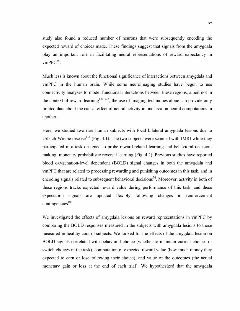
97

study also found a reduced number of neurons that were subsequently encoding the

expected reward of choices made. These findings suggest that signals from the amygdala

play an important role in facilitating neural representations of reward expectancy in

vmPFC55.

Much less is known about the functional significance of interactions between amygdala and

vmPFC in the human brain. While some neuroimaging studies have begun to use

connectivity analyses to model functional interactions between these regions, albeit not in

the context of reward learning131-133, the use of imaging techniques alone can provide only

limited data about the causal effect of neural activity in one area on neural computations in

another.

Here, we studied two rare human subjects with focal bilateral amygdala lesions due to

Urbach-Wiethe disease134 (Fig. 4.1). The two subjects were scanned with fMRI while they

participated in a task designed to probe reward-related learning and behavioral decision-

making: monetary probabilistic reversal learning (Fig. 4.2). Previous studies have reported

blood oxygenation-level dependent (BOLD) signal changes in both the amygdala and

vmPFC that are related to processing rewarding and punishing outcomes in this task, and in

encoding signals related to subsequent behavioral decisions74. Moreover, activity in both of

these regions tracks expected reward value during performance of this task, and these

expectation signals are updated flexibly following changes in reinforcement

contingencies109.

We investigated the effects of amygdala lesions on reward representations in vmPFC by

comparing the BOLD responses measured in the subjects with amygdala lesions to those

measured in healthy control subjects. We looked for the effects of the amygdala lesion on

BOLD signals correlated with behavioral choice (whether to maintain current choices or

switch choices in the task), computation of expected reward value (how much money they

expected to earn or lose following their choice), and value of the outcomes (the actual

monetary gain or loss at the end of each trial). We hypothesized that the amygdala

98

contributes to computations of expected reward value in vmPFC, which in turn should

affect signals of behavioral choice.

99

RESULTS

Subjects

Both amygdala subjects had focal bilateral lesions in the amygdala due to Urbach-Wiethe

disease (Fig. 4.1). One of the subjects, S.M., has been extensively published before: she is a

41-year-old woman with a high-school education, IQ in the normal range, and normal basic

visuoperception, language, and memory; her lesions encompass the entire amygdalae, as

well as subjacent white matter and very anterior entorhinal cortex. The second subject,

A.P., is a 21-year-old woman in college with likewise normal IQ, perception, language, and

memory; lesions are entirely confined to the amygdala, occupying roughly 50% of each

amygdala’s volume. Both subjects are fully right-handed, live independently, and show no

evidence of psychopathology on tests of personality assessment. Both subjects also perform

normally on standard neuropsychological tests of response switching, such as the

Wisconsin Card Sorting Task and the Trailmaking task. Subjects with amygdala lesions

were compared to 16 healthy controls of similar age as A.P. (Controls), as well as to 4

healthy women similar to S.M. in age (SM-comparisons, see Methods for further details).

Behavioral performance on probabilistic reversal learning

Subject AP

AP was significantly impaired relative to controls in the average number of trials to reach

the criterion for contingency reversal, and hence impaired in the number of contingency

reversals obtained over the course of the task. AP obtained only 3 reversals, whereas

controls obtained on average 8 reversals, a performance 3.5 S.D.s below the control mean

(p<0.002). A further analysis of AP’s performance revealed that, although she was not

significantly more likely to switch choice when compared to controls (Fig. 4.3), her choice

of when to switch was inconsistent with the reward contingency: in particular, she switched

choice after obtaining a positive reward much more often than did the controls. For this

reason, although she switched the same amount as controls did overall, she achieved fewer

contingency reversals in the task.

100

Subject SM

SM was also impaired relative to controls in the number of contingency reversals,

obtaining 4 reversals. However, the SM-comparison subjects who were closer in age to SM

were also variably impaired relative to the control group, and when SM’s data were

compared to this group of subjects of more similar age, her behavioral variables did not

stand out as abnormal (Fig. 4.3). It should be noted that for the purpose of our fMRI study,

the fact that SM performs similarly to SM-comparison subjects is in fact advantageous, as

any observed differences in BOLD signal would then be unlikely to be confounded by

differences in behavior135.

Both amygdala lesion subjects were also impaired in the number of trials taken to reach

acquisition during the initial training phase outside the scanner (even before reversals took

place). However, as in the behavioral performance during scanning itself, the SM-

comparison subjects were also impaired relative to the younger controls (see Fig. S4.1).

fMRI Results

Here we report whole brain analyses of BOLD signal correlating with parameters from our

models that are based on the behavior of the control subjects, but restrict our analysis of the

difference in BOLD signal between amygdala lesion subjects and controls to those regions

that originally elicited a signal in controls—notably, specific regions of prefrontal cortex

(see Methods). fMRI data for this same set of control subjects is more extensively analyzed

in Hampton et al.109.

Behavioral choice signals

In order to determine the effects of amygdala lesions on BOLD signals in orbital and

medial prefrontal cortex related to behavioral choice, we first conducted a simple canonical

trial-based analysis of the fMRI data whereby we examined BOLD responses following

receipt of the outcome on a given trial (as in O’Doherty et al.74). Trials were separated

according to whether on the subsequent trial following the outcome subjects changed their

choice of stimulus (“switch” trials) or continued choosing the same stimulus (“stay” trials).

101

Fig. 4.4A shows areas with significant responses in “switch” compared to “stay” trials in

control subjects. This contrast revealed significantly greater activity in “switch” compared

to “stay” in anterior frontal insula, extending into posterior lateral orbitofrontal cortex and

anterior cingulate cortex (ACC). The reverse contrast revealed significant effects in mPFC

(Fig. 4B). These results are consistent with previous studies of reversal learning in healthy

control subjects74, 75, 86.

Differences in behavioral choice signals in amygdala subjects compared to controls

We examined regions in which the above contrast would differ between our two subjects

with amygdala lesions and controls by restricting the analysis to those voxels that showed a

significant effect in the controls in the first place (for switch-stay; Fig. 4.4A). We found

significantly greater responses in switch compared to stay trials in control subjects than in

the two amygdala subjects in a region of posterior lateral orbitofrontal cortex/anterior

insula, bilaterally (Fig. 4.4C, threshold at p<0.01). These differences were significant in

each amygdala subject individually compared to controls (at p<0.001 for SM and at p<10-8

for AP). A plot of the contrast estimates for switch-stay are shown in Fig. 4.4D. It is

notable that responses in both amygdala subjects are markedly different from controls, and

even from the SM-comparison subjects (who were similar in their behavioral performance

to SM). A comparison of the reverse contrast (stay-switch) between amygdala subjects and

controls did not reveal any significantly decreased responses in the amygdala subjects.

These results indicate that bilateral damage to the amygdala results in altered responses in

anterior insula/posterior orbitofrontal cortex and anterior cingulate cortex related to

behavioral choice, suggesting that in healthy individuals the amygdala makes an important

contribution to the computation of behavioral control signals in those regions.

Expected reward signals

We next examined BOLD responses to expected reward. For this, we applied a

computational model which calculates expected reward signals related to subjects’ choice

in a trial by taking into account the history of rewards and punishments obtained and the

history of choices made (see Methods). In our control subjects, we found significant

102

correlations with this signal in orbital and medial prefrontal cortex (Fig. 4.5A), time locked

to the time of choice. Activity in these areas increases in a linear fashion as a function of

increasing expected reward value109 suggesting that these areas are involved in encoding

the expected reward of the currently chosen stimulus.

Differences in expected reward signals between amygdala subjects and controls

In a direct comparison between areas correlating with expected reward signals in the

amygdala subjects and controls, we found significant differences in medial prefrontal

cortex at p<0.001 (Fig. 4.5B). These results were significant in each subject individually

when compared to controls at p<0.001 for AP and p<0.0001 for SM. A consistent

difference between AP and controls, and between SM and SM-comparison subjects can be

seen when plotting the regression coefficients of all subjects in medial prefrontal cortex

(Fig. 4.5C), confirming that the amygdala subjects process the expected reward value of

each choice abnormally. These results were obtained by fitting a model to the behavior of

the group of 16 controls, and then using the model parameters as the regressor against the

fMRI data from the amygdala subjects, as well as the fMRI data from the controls.

However, in order to account for the possibility that a difference in model parameters

between the controls and amygdala subjects could account for the above results, we also

performed the same analysis using parameter fits derived individually from each of the

amygdala subjects. This analysis yielded the same results: a significant difference in

expected reward signals in medial prefrontal cortex in amygdala subjects compared to

controls (Fig. S4.2A).

To further characterize how amygdala lesion subjects process expected reward

representations in medial prefrontal cortex, we plotted the signal in medial PFC measured

with fMRI against the expected reward signals obtained from the model of the subjects’

task performance. We sorted trials into one of 5 bins to capture different ranges in the

expected reward values and fitted each bin separately to the fMRI data. For controls, this

analysis shows a linear increasing relationship between the magnitude of the evoked fMRI

signal in this region and expected reward value. By contrast, responses in mPFC in the

103

amygdala subjects did not display a clear linear increasing relationship with expected

reward (Fig. 4.5D).

Responses to rewarding and punishing outcomes

We also looked for responses relating to the receipt of rewarding or punishing feedback at

the time of outcome. In our control subjects, when comparing responses to receipt of

rewarding compared to punishing outcomes, we found significant activity relating to

receipt of reward in medial prefrontal and medial orbitofrontal cortex (Fig. 4.6A),

consistent with previous reports53, 74, 136-138. On the other hand, when testing for areas

responding to punishing compared to rewarding outcomes we found significant effects in

the anterior ventrolateral prefrontal cortex extending into lateral OFC, also consistent with

previous results53, 139, 140.

Differences in responses to rewarding and punishing outcomes in amygdala subjects

compared to controls

We then compared the above contrast in amygdala subjects to that in the control subjects,

again restricting ourselves to those regions that showed significant effects (at p<0.01) of

rewarding or punishing feedback in the control subjects in the first place. We found no

significant differences in BOLD responses to rewarding or punishing feedback in amygdala

subjects compared to controls at p<0.001 uncorrected, with only a single voxel surviving in

medial PFC in the reward contrast at p<0.01 (Fig. 4.6B). These results suggest that

processing of rewarding and punishing feedback in OFC and medial PFC remains intact

after amygdala lesions. Thus, amygdala lesions appear to impair selectively the generation

of behavioral choice and expected reward signals in prefrontal cortex, but leave the

generation of reward outcome signals relatively unaffected.

Controlling for behavioral differences between amygdala subjects and controls

In order to further control for the possibility that differences in behavior between the

amygdala subjects and controls could contribute to the results observed, we performed a

follow-up analysis in which we selected only those trials on which every subject had made

a correct choice according to the underlying task contingency. That is, we chose those trials

104

on which subjects correctly maintained their choice of stimulus (if their current choice of

stimulus was correct), and those trials on which subjects correctly switched their choice of

stimulus after the contingencies had reversed. All other trials were modeled separately as

error trials of no interest. We then conducted the same analyses reported above for each

contrast of interest. All of the above results held up (see Figs. S4.2B and S4.3), indicating

that the abnormal signal in prefrontal cortex that we report following amygdala damage

cannot be due simply to differences in the distribution of errors made between controls and

amygdala subjects.

105

DISCUSSION

Amygdala and ventromedial prefrontal cortex are known to play an important role in

reward-related learning and decision making, yet little is known about how these structures

interact to support such functions in the human brain. In the present study, we provide

novel evidence that neural representations in orbital, medial, and lateral prefrontal cortex

related to the computation of expected reward and the computation of behavioral choice

depend on input from the amygdala. Moreover, our results indicate that reward outcome

representations in vmPFC are not as dependant on amygdala input.

Consistent with previous reports74, 75, we found robust signals related to behavioral choice

in posterolateral OFC, agranular insula, and anterior cingulate cortex in healthy individuals.

By contrast, these signals were significantly reduced in both subjects with amygdala

lesions. Moreover, this effect is unlikely to be driven by differences in behavioral

performance between the amygdala subjects and their controls, as these results held up

even when behavioral differences between the patients and controls were taken into

account in the fMRI analysis (by restricting analysis to only those trials in which both

amygdala subjects and controls made the correct choices). Furthermore, subject SM did not

show overall behavioral impairments relative to her age-matched comparison subjects, yet

still showed significant differences in activity in the target regions of prefrontal cortex

compared to controls. Thus, differences in neural signals in this area are unlikely to be

merely a consequence of the degree of behavioral impairment on the task, but are likely to

be a direct consequence of the amygdala lesion. These results support the hypothesis that

the production of signals related to behavioral choice in OFC and anterior cingulate cortex

relies directly on input from the amygdala.

This conclusion leaves open the question of what precisely the amygdala contributes to

behavioral choice signals in prefrontal cortex. Computational models of decision-making

such as those grounded in reinforcement learning approaches, conceive of behavioral

decision-making as being driven by an underlying computation of expected rewards or

utilities for different available actions or stimuli. Decisions are then weighted according to

the relative value of the different actions, so that over the course of learning choices

106

associated with higher value become favored (with the caveat that actions believed to be

sub-optimal nonetheless may sometimes be selected for the purposes of exploration17). The

decision process is likely therefore to involve an explicit comparison between expected

reward values available for different actions. In the case of reversal learning, there are only

two possible actions: either maintaining current behavioral choice when the chosen

stimulus is believed to be correct, or switching stimulus choice once a change in

contingencies has been detected. Here we used a computational model of decision-making,

which is essentially a modified reinforcement learning algorithm that also takes into

account the reversal structure of the task. This model computes expected reward signals

based on the history of prior outcomes. Previously we have shown that BOLD signals in

ventromedial prefrontal cortex reflect computations of expected reward according to this

model109. We hypothesize that these expected reward signals are then used as input to the

decision-making process in order to determine whether to maintain current stimulus choice

or switch stimulus choice in the task.

In the present study we found that expected reward signals in medial PFC were markedly

abnormal in the amygdala lesion subjects. Whereas control subjects showed a linear

increase in activity in this region as a function of increased expected reward value, no such

relationship was found in the subjects with amygdala lesions. The absence of normal

expected reward signals in the medial PFC of subjects with amygdala lesions implies that

these signals can no longer be used appropriately to generate behavioral decisions. The lack

of these expected reward signals could therefore also account for the difference in observed

behavioral choice signals. Thus, we suggest that the primary contribution of amygdala-

vmPFC interactions is in computing expected reward values which, once established, are

then used to generate behavioral decisions.

While we found significant effects of amygdala lesions on prefrontal signals of expected

reward and behavioral choice, we found no such effects on signals of receipt of the

outcome. In control subjects, receipt of monetary reward elicited robust signal in medial

prefrontal cortex extending down to the medial orbital surface, consistent with many

previous findings53, 137, 139. However, when comparing BOLD signal in controls to that in

107

amygdala lesion subjects, we found no significant differences, except for a single voxel at

p<0.01, suggesting that differential processing of reward feedback in this area is unaffected

by the lesion. Similarly, BOLD signal to punishing feedback was found in lateral areas of

prefrontal cortex (on the lateral surface and extending down to lateral OFC) in controls,

again consistent with prior observations. However, once again there were no differences

between activity in amygdala subjects and controls in these responses. Thus, our findings

indicate that amygdala lesions selectively impair some but not all aspects of reward-related

processing in vmPFC, ruling out a non-specific effect of amygdala lesions on vmPFC

function or on the BOLD signal in general.

To conclude, the results of the present study highlight an important contribution of

amygdala-vmPFC interactions toward the computation of expected reward value in

humans, and support a model of decision making whereby these expected reward signals,

once computed, are integrated in vmPFC and then subsequently used to guide behavioral

decision making. More generally, these results highlight the utility of combining studies of

human subjects who have discrete lesions with neuroimaging in order to address

computationally-driven hypotheses about the functional significance of neural interactions

between brain areas. While the present study has addressed the role of amygdala lesions on

vmPFC function, a fruitful avenue for future research will be to investigate the converse

effects of vmPFC lesions on amygdala function, and to explore interactions with additional

structures involved in reward processing, such as the ventral striatum.

108

MATERIALS AND METHODS

Subjects

Two subjects with bilateral amygdala lesions (AP: age 20, Full-Scale IQ 98, VIQ 92, PIQ

106; and SM: age 42, Full-Scale IQ 88, VIQ 86, PIQ 95) participated in this study141.

Sixteen healthy, normal subjects also participated as controls (8 female, 14 right handed),

as well as four subjects similar to SM in age and IQ (all female, mean age 53±7, mean IQ

99±4). Control subjects excluded those with a prior history of neurological or psychiatric

illness. All subjects gave informed consent and the study was approved by the Institutional

Review Board at Caltech. Before entering the scanner, subjects were informed that they

would receive what they earned (or lost) in the task, added to an initial amount of $25

dollars. It was not possible for subjects to produce a net monetary loss in the study.

Pre-scan training

Before scanning the subjects were trained on three different versions of the task. The first is

a simple version of the reversal task, in which one of the two fractals presented yields

monetary rewards 100% of the time and the other monetary losses 100% of the time. These

then reverse according to the same criteria as in the imaging experiment proper, where a

reversal is triggered with probability 0.25 after 4 consecutive choices of the correct

stimulus. This training phase is ended after subjects successfully complete 3 sequential

reversals. The second training phase consists of the presentation of two stimuli that deliver

probabilistic rewards and punishments as in the experiment (see Fig. 4.2), but where the

contingencies do not reverse. The training ends after the subject consecutively chooses the

“correct” stimulus 10 times in a row. The final training phase consists of the same task

parameters as in the actual imaging experiment (stochastic rewards and punishments as

described in the main text, and stochastic reversals). This phase ends after the subject

successfully completes 2 sequential reversals. Different fractal stimuli were used in the

training session than those used in the scanner. Subjects were informed that they would not

receive remuneration for their performance during the training session. Subject

performance during training can be seen in Fig. S4.1.

109

Data acquisition and pre-processing

Blood oxygenation level dependent (BOLD) functional MRI was conducted using a

Siemens 3.0 Tesla Trio MRI scanner to acquire gradient echo T2* weighted echo-planar

images (EPI). An eight-channel phased array head coil was used for radiofrequency

reception. Visual stimuli were presented using Restech (Resonance Technologies,

Northridge, CA, USA) goggles, and subject responses were recorded with a button box.

Oblique axial-coronal slices were acquired at 30° to the AC-PC line for a neutral head

position to minimize signal loss and geometric distortion in the orbitofrontal cortex (OFC).

A total of 580 volumes (19 minutes) were collected during the experiment in an

interleaved-ascending slice order. The imaging parameters were: echo time (TE), 30ms;

field-of-view (FOV), 192mm; in-plane resolution and slice thickness, 3mm; repetition time

(TR), 2 seconds. Whole-brain, high-resolution T1-weighted structural scans (1x1x1mm)

were also acquired from the control subjects, co-registered with their mean EPI and

averaged to permit anatomical localization of the functional activations at the group level.

Image analysis was performed using SPM2 (Wellcome Department of Imaging

Neuroscience, Institute of Neurology, London, UK). Temporal normalization was applied

to the scans, each slice being centered to the middle of the scan (TR/2). To correct for

subject motion, all EPI volumes were realigned to the first volume, spatially normalized to

a standard T2* template with a resampled voxel size of 3mm, and spatially smoothed using

a Gaussian kernel with a full width at half maximum (FWHM) of 8mm. Intensity

normalization and high-pass temporal filtering (using a filter width of 128 secs) were also

applied to the data96. The same process was applied to the amygdala lesion subjects, and no

qualitative spatial distortion effects due to the normalization process could be seen near the

lesioned area in either the functional EPI or structural T1-weighted scans.

Data Analysis

Behavioral Data

To compare the behavior of the amygdala lesion subjects in the probabilistic reversal task

to control subjects, we analyzed two measures: First, how often do subjects switch choice

(depending on whether they have just received a reward or a punishment); and second, how

many task contingency reversals does their behavior elicit, given that subjects have to reach

110

the criterion of making the correct choice four times in a row before task contingency

probabilistically reverses. For statistical comparisons across subjects, these measurements

are assumed to have a binomial distribution for each individual subject, and are modeled as

a beta distribution across subjects (the beta distribution being a conjugate prior distribution

of the binomial distribution142). Behavioral statistical significance t-scores (Fig. 4.3) of the

difference between each amygdala lesion subject and control subjects were appropriately

corrected to take into account that measurements have a beta distribution instead of a

Gaussian distribution.

Computational model-based analysis: generating expected reward signals

In order to generate signals related to subjects’ expected reward value on each trial we used

an approximation to the Hidden Markov Model formulation used previously109, whereby in

order to choose optimally, it is necessary to compute expected reward signals not only by

taking into account the history of rewards and punishments received on a given choice, but

also the structure of the task: namely, that when one choice is correct, the other is not (this

derivation is further detailed in Appendix B). Rewards and punishments received on each

trial were used to update both the selected and unselected choices. Thus, after making

choice A and receiving a reward, the update of the value of both choices becomes:

)(

)(1

1

tB

ttB

tB

tA

ttA

tA

VRVV

VRVV

−−+=

−+=+

+

η

η

(4.1)

where tA

t VR − is the prediction error between the reward tR subjects obtained at time t,

and the expected reward tAV of their choice. This model is therefore a variant of standard

reinforcement learning, except for the additional updating of the action not taken (action

B), similar to fictive updating in RL143, 144. This model states that subjects assume that the

reward they would have received for the choice not taken is exactly opposite to the reward

they receive for their current choice. Although reward outcomes are probabilistic, this

update correctly captures the anti-correlation between choice values in this task.

111

To choose which action to make (A or B), the model compares their expected rewards to

select which will give the most reward in the future. The probability of choosing action A

is:

{ }( )αβσ −−= )()( AB VVAP (4.2)

where ))exp(1/(1)( zz +=σ is the Luce choice rule18 or logistic sigmoid, α indicates the

indecision point (when it’s equiprobable to make either choice) and β reflects the degree of

stochasticity in making the choice (i.e., the exploration/exploitation parameter).

In order to estimate the free parameters in the model, we fit the model predictions to

subjects’ actual behavior data, and selected those parameters which minimized the error in

the fit of the model to the behavioral data (using logistic log likelihood errors). We used the

multivariate constrained minimization function (fmincon) of the Optimization Toolbox 2.2

in Matlab 6.5 (www.mathworks.com) for this fitting procedure.

FMRI data analysis

Behavioral choice

For the analysis of behavioral choice signals, we conducted an analysis similar to that

reported in O’Doherty et al.74. For this, we categorized trials according to subjects’ reward

outcomes and subsequent behavioral choices. We modeled event-related responses at the

time of receipt of the outcome, and differentiated between trials in which subjects

subsequently switched their choice of stimulus (switch trials), and trials in which subjects

maintained their current choice of stimulus (stay trials). These two type of trials were

further differentiated by whether subjects received a punishment or a reward as a

consequence of their choice in the current trial. Separate regressors were entered for

reward-stay, reward-switch, punish-stay, and punish-switch trials, by constructing sets of

delta (stick) functions at the time of the outcome for each trial type. A common regressor

across all trial types was also modeled at the time of choice. These regressors were then

convolved with a canonical hemodynamic response function. In addition, the 6 scan-to-

scan motion parameters produced during realignment were included to account for residual

112

motion effects. These regressors were fitted to each subject’s fMRI data individually, and

the regression parameters were then taken to the random effects level, to generate group

random effects statistics. The regression parameters for both amygdala subjects were

modeled separately at the random effects level from the regression parameters for the

control subjects. A linear contrast was then computed between the amygdala subjects and

controls to identify areas showing significant differences between amygdala subjects and

controls. For the results reported in the present study, we tested for areas showing

significantly decreased responses in the amygdala subjects compared to the controls at

p<0.001 uncorrected in our regions of interest, restricted to those areas showing significant

effects for the switch-stay contrast in the control subjects (at p<0.01 or lower). The results

were also masked to show only those voxels that are significantly different to controls in

each amygdala lesion subject individually (at p<0.05 or lower), in order to select only those

areas that are significantly different in both subjects compared to controls.

Expected reward signals

We then conducted an additional analysis to detect brain regions correlating with expected

reward. For this, regressors were constructed using the trial-by-trial expected reward

signals as predicted by the computational model described above, given the trial history of

each individual subject. These were then entered as parametric regressors set at the time of

choice. We also modeled the outcome received on each trial (whether a reward or a

punishment was obtained). As before, these regressors were convolved with a

hemodynamic response function, and motion regressors were included as effects of no

interest.

These regression fits were then taken to the random effects level separately for the contrasts

of expected reward signals at the time of choice and rewards vs. punishments at the time of

outcome, and a comparison was computed between both amygdala subjects and controls

for each contrast separately. Statistical significance was reported at p<0.001 uncorrected in

our regions of interest. As before, we restricted our analysis to those voxels showing

significant effects in the relevant contrast in the controls (at p<0.01 or below), and show

113

only those voxels that surviving a comparison of each individual amygdala subject to

controls significant at p<0.05 or lower.

SM AP Control

114

115

Figure 4.1. Axial T1-weighted structural MR images from the two amygdala lesion

subjects. Selective bilateral calcification of the amygdala (arrows) due to Urbach-Wiethe

disease134 is evident as loss of signal on these T1-weighted structural MR scans of the

brains of S.M. (left) and A.P. (middle). An image from a typical healthy control subject

with intact amygdalae is also shown for comparison (right). Multiple axial slices for both

amygdala lesion subjects are shown in Fig. S4.4.

++

++

++

$2.50$2.50

Trial Onset

~500msSubject makeschoice

5000msReward delivered

7000ms Trial ends

116

117

Figure 4.2. Probabilistic reversal task. Subjects chose one of two fractals, which on each

trial were randomly located to the left or right of a fixation cross. Once a stimulus was

selected by the subject, it increased in brightness and remained on the screen for a total of 2

seconds. After a further 3s blank screen, a reward (winning 25 cents, depicted by a quarter

dollar coin) or punishment (losing 25 cents, depicted by a quarter dollar coin covered by a

red cross) was shown, with the total money earned displayed at the top ($2.50 in this

figure). One stimulus was designated as the correct stimulus and resulted in a monetary

reward on 70% of occasions, and a monetary loss 30% of the time, with an overall

accumulation of monetary gain in the task. The other, “incorrect” stimulus resulted in a

reward 40% of the time and a punishment 60% of the time, with a cumulative monetary

loss. After subjects chose the correct stimulus on 4 consecutive occasions, the

contingencies reversed with a probability of 0.25 on each successive trial. Subjects had to

infer that the reversal took place and switch their choice, at which point the process was

repeated.

0

1

2

3

4

AP SM SM Com.

T-s

core

AP SM SM Com.

Trials to reach criteria Number of switches

0

1

2

3

4

118

119

Figure 4.3. Behavioral performance. During the reversal task performed in the scanner,

both AP and SM took more trials to reach reversal criteria than controls (left panel – AP

p<.002, SM p<.02). This was not directly caused by the number of choice switches the

amygdala subjects executed (right panel), for AP did not significantly switch more often

than controls did. However, the “quality” of these decisions was arguably impaired, in that

the amygdala subjects would switch choice more often than controls in situations when it

was not advantageous to do so, such as switching choice after receiving a rewarding

outcome. However, controls of similar age to SM (right column in both panels; bar shows

means, yellow symbols show individual data) were also impaired on these measures,

compared to the younger controls.

-3

0

3

A Switch-stay controls B Stay-switch controls

C Controls > amygdala (sw-st)

P<.01p<.001

Insula ACC

Sw

itch

-Sta

y C

on

tra

st

D

ControlsSM Com.SMAP

X= -30

X= -28

X= -9

X= -11

Y=+46

120

121

Figure 4.4. Behavioral choice signals. Contrast (aligned to the time of outcome) between

trials for which subjects subsequently switch their choice of stimulus (“switch”), compared

to trials for which subjects subsequently continue choosing the current stimulus (“stay”).

(A) Regions showing increased BOLD signal on “switch” compared to “stay” trials in

control subjects. Significant effects were observed in anterior frontal-insula/posterior lateral

orbitofrontal cortex bilaterally (-30, 21, -9mm, z=3.91 and 33, 21, -12mm, z=3.64), anterior

cingulate cortex (-9, 21, 33mm, z=3.62), and extending into pre-motor cortex (0, 18,

51mm, z=3.73). (B) Regions showing increased BOLD signal on stay compared to switch

trials. Significant effects were observed in mPFC (-6, 45, 21mm, z=3.79). (C) Both

amygdala subjects had significantly less switch vs. stay activity than controls in posterior

lateral orbitofrontal cortex/anterior insula bilaterally (-30, 21, -18mm, z=4.2 and 36, 21,

-18mm, z=4.32) and ACC (-9, 33, 42mm, z=5.29). (D) Switch-stay contrasts in both these

areas show that not only are both amygdala subjects significantly different from the 16

younger controls as well as the SM-comparison subjects, but also that the control group

shows a very similar signal to the SM-comparisons. This is in stark contrast with the

behavioral results, where SM-comparisons were also impaired when compared to the

younger controls. Thus, behavioral differences are not driving the differences in fMRI

signal.

-20

-10

0

10

20

A Expected reward (controls)

B Controls > amygdala (exp. rew.) C

Re

gre

ssio

n C

oe

ffic

ien

t

p<.01p<.001

ControlsSM Com.SMAP

Y=-6 Y=+52 Y=+66

Y=+66Y=+57

-2

-1

0

1

2

low high low highExpected reward

Re

gre

ssio

n C

oe

ffic

ien

t

D Expected reward in mPFC

-2

-1

0

1

2

Expected reward

medial PFC

122

123

Figure 4.5. Expected reward signals in the brain. (A) For control subjects, BOLD signal

correlating with the magnitude of expected reward of a choice was found in ventromedial

prefrontal cortex (6, 57, -6mm, z=5.13) and the amygdala bilaterally (-27, -6, -21mm,

z=3.89) extending into hippocampus109. (B) We found a significantly weaker correlation

with expected reward signal in mPFC (6, 57, -3mm, z=4.12) in the two amygdala subjects

compared to controls (at p<0.001). (C) Regression coefficients in mPFC (6, 57, -3mm)

indicate that both amygdala subjects differ markedly from controls in their representation

of expected rewards, and SM differs with respect to SM-comparison subjects as well. (D)

To analyze the relationship between expected rewards and BOLD signal in medial PFC, we

subdivided trials into five bins depending on the expected reward value on that trial. The

regression coefficients for each bin are plotted for the control subjects and for the SM-

comparison subjects (left panel), showing the linear relationship between expected rewards

and brain BOLD activity. However, in contrast to the controls, the relationship between

expected rewards and BOLD activity for both amygdala lesion subjects is nearly flat,

indicating that both subjects are not computing expected rewards in mPFC in the same way

as controls. Regression coefficients were extracted at the local maximum of the expected

reward contrast for each subject, within a 10 mm radius of the group peak (as shown in

panel B).

A Controls

B Controls > amygdala

p<.01p<.001

Rew - Pun Pun - Rew

Rew - Pun Pun - Rew

Y=+52 Y=+52

Y=+57

124

125

Figure 4.6. Responses to receipt of rewarding and punishing outcomes. (A) In a direct

comparison of BOLD responses to rewarding and punishing outcomes in control subjects,

we found increased activity in medial OFC to receipt of rewarding compared to punishing

outcomes (-3, 57, -9mm, z=4.23), and increased activity in anterior ventrolateral prefrontal

cortex extending into far lateral OFC to the receipt of punishing outcomes (27, 52, 6mm,

z=3.45). (B) However, in a direct comparison of responses to rewarding outcomes between

the amygdala lesion subjects and controls, we found no significant differences (except one

voxel at p<0.01 in mPFC). Similarly, no differences were found in BOLD signal responses

to punishing outcomes between amygdala subjects and controls. This suggests that

outcome representations in orbital, medial, and lateral prefrontal cortices are unaffected by

the amygdala lesions.

T-s

core

0

1

2

3

4

Acquisition performance

Trials to reach criteria Number of switches

AP SM SM Com. AP SM SM Com.

0

1

2

3

4

126

127

Figure S4.1. Subject performance during task acquisition. During training, subjects

were exposed to a version of the task where one choice was always on average rewarding

while the other was always on average punishing (see Methods). Both amygdala lesion

subjects took a larger number of trials to reach the criteria of choosing the correct stimulus

(by making the correct choice ten times in a row, or reaching the maximum number of

trials allocated to this training phase). This is shown on the left panel, which shows a

comparison of the number of trials taken to finish training for amygdala subjects and SM-

comparison subjects (individual subjects marked with yellow rhomboids), when compared

to controls. Furthermore, amygdala subjects and SM-comparison subjects switched their

choice of stimulus more often on average than controls did (right panel).

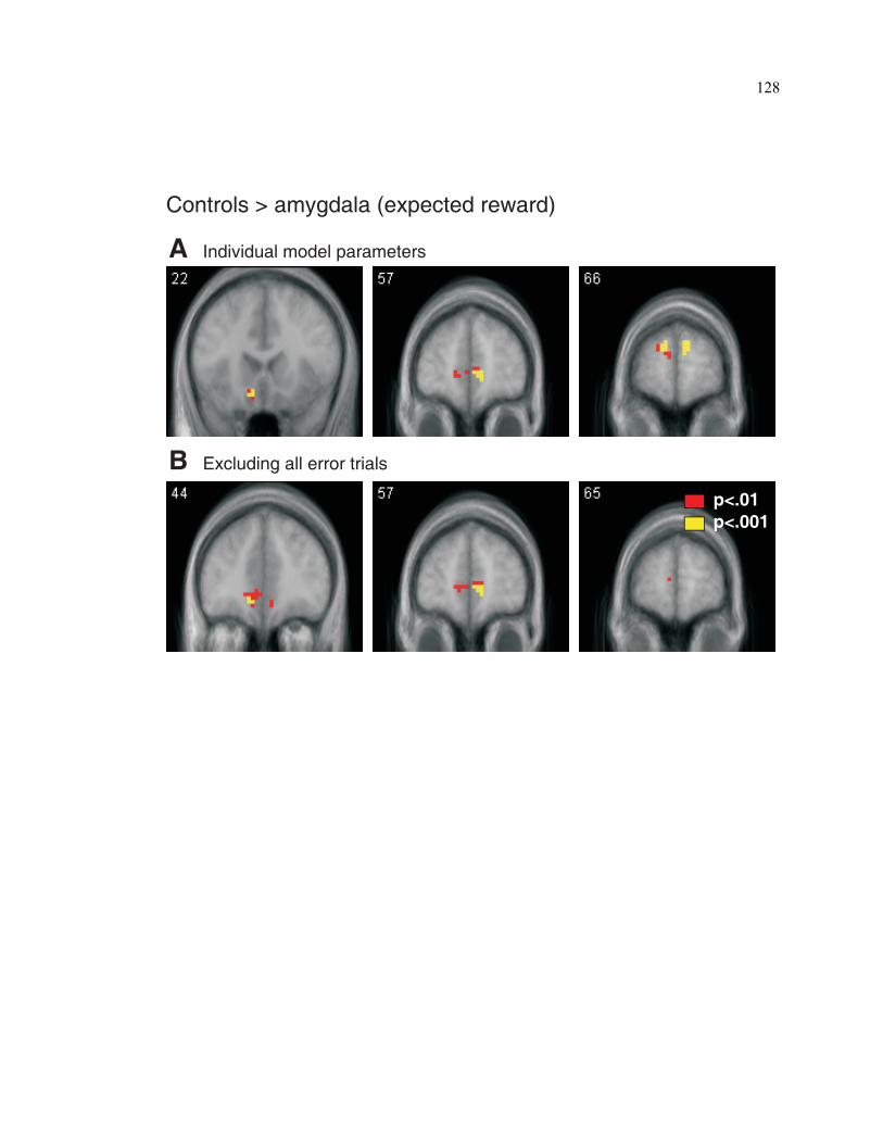
Controls > amygdala (expected reward)

B Excluding all error trials

A Individual model parameters

p<.01p<.001

128

129

Figure S4.2. Controlling for the effects of behavioral differences between amygdala

subjects and controls on signals pertaining to expected reward value. To control for the

effects of differences in behavioral performance between the amygdala subjects and control

subjects on the fMRI results for the comparison of expected reward signals (Fig. 4.5B), we

performed two additional tests: (A) We first compared expected reward signals between the

amygdala subjects and controls, but this time with model parameters derived from the best

log likelihood fits of the computational model to the behavioral data for each amygdala

subject individually. This controls for the possibility that the model accounts equally well

for the behavioral data in the amydala lesion subjects as the controls, but that the amygdala

subjects and controls only differ in the model-parameters. Contrary to this possibility, this

analysis still revealed significant differences between amygdala subjects and controls in

expected reward signals (again at p<0.001), again consistent with the results reported in the

this chapter. (B) We then compared expected reward signals between the two amygdala

subjects and controls using only those trials for which subjects made correct choices given

the underlying contingencies. Here, we used the model-parameters derived from the control

subjects. Consistent with the results reported previously (Fig. 4.5B), this analysis still

showed significant differences between amygdala subjects and controls in encoding of

expected rewards in medial PFC at p<0.001.

Controls > amygdala (switch-stay)

X= -28X= -11

p<.01p<.001

130

131

Figure S4.3. Controlling for behavioral differences between amygdala lesion subjects

and controls in signals pertaining to behavioral choice. To further control for the effects

of differences in behavioral performance between the amygdala subjects and control

subjects on the fMRI data, we restricted our analysis to only those trials in which both

amygdala subjects and controls made correct choices (given the underlying contingencies).

For this, we modeled separately trials in which subjects’ action of staying with the same

choice, or switching choice was correct given the underlying task contingency, from trials

in which subjects’ actions were incorrect given the underlying task contingency. In this

figure we show the results of a comparison between switch-stay trials in amygdala subjects

and controls, similar to that shown in Fig. 4.4C. Even after controlling for behavioral

differences, this analysis revealed a similar result to that reported in Fig. 4.4C. That is,

amygdala subjects showed significantly reduced activity in posterior lateral orbitofrontal

cortex/anterior insula and anterior cingulated cortex on switch-stay trials compared to

controls (an effect which was still significant at p<0.001).

SM

AP

*

*

132

133

Figure S4.4. Multiple axial slices for both amygdala lesion subjects. Multiple axial

slices of un-normalized T1-weighted structural images for both amygdala lesion subjects

show that the rest of the brain is generally unaffected by the disease. Axial slices marked

with an asterisk are shown in Fig. 4.1, in which the amygdala lesions for both subjects are

compared to the intact amygdala of a typical control subject. In the asterisk-marked slices,

the bilateral calcification of the amygdala due to Urbach-Wiethe disease can be seen as a

loss of signal (dark) on these T1-weighted structural MR scans.

134

C h a p t e r 5

THINKING OF YOU THINKING OF MEvi

Competing successfully with an intelligent adversary depends on the ability to mentalize

the opponent’s state of mind in order to anticipate the opponent’s behavior in the future.

Here, we explore the computational underpinnings of such a capacity by scanning human

subjects with fMRI while they engaged in a simple strategic game against a real opponent.

Subjects were found to employ a sophisticated strategy, whereby they used knowledge of

how their actions would influence the actions of their opponent to guide their choices.

Moreover, specific computational signals required for the implementation of such a

strategy were present in medial prefrontal cortex and superior temporal sulcus, providing

insight into the basic computations underlying competitive strategic interactions, and their

associated neural bases.

vi Work done in collaboration with Peter Bossaerts and John P. O’Doherty.

135

Humans, like many other primates, live in a highly complex social environment in which it

is often necessary to interact with, and compete against, other individuals in order to attain

reward. Success against an intelligent adversary with competing objectives likely depends

on the capacity to infer the opponent’s state of mind, in order to predict what action the

opponent is going to select in future and to understand how an individual’s own actions

will modify and influence the behavior of one’s opponent. This ability is often referred to

as “mentalizing” and has been linked to a number of specific regions thought to be

specifically engaged when processing socially relevant stimuli, and especially when

inferring the state of mind of others145. Neuroimaging studies in humans have implicated a

specific network of brain regions including dorsomedial prefrontal cortex, posterior

superior temporal sulcus (STS), and the temporal poles146, 147 while subjects engage in tasks

relevant to mentalizing, such as evaluating false beliefs or social transgressions148, 149,

describing the state of biological movements150-152, and while playing interactive games153-

155. However, although these studies have provided insight into what brain regions may be

involved in the capacity to mentalize, the question of how this function is implemented at

the neural level has received relatively little attention to date.

The goal of the present study was to begin to characterize the basic computational signals

underlying the capacity to mentalize, and to link different components of these putative

signals to specific brain regions. In order to assess competitive interactions experimentally,

we studied pairs of human subjects while they played each other in a two-player strategic

game called the “inspection” game (or generalized matching pennies), in which opponents

have competing goals (Figure 5.1A and 5.1B). One of the players was being scanned with

fMRI, while their opponent was playing outside the scanner. The “employer” could either

“inspect” or “not inspect,” while the “employee” could either “work” or “shirk.” The

employer received 100 cents if he/she did “not inspect” and the employee “worked,” and

received 25 cents if he/she “inspected” and caught the employee “shirking.” Otherwise

he/she got zero cents. In contrast, the “employee” got 50 cents for “working” when the

employer “inspected,” and for “shirking” when the employer did “not inspect,” otherwise

getting zero cents as well. Both players had competing objectives, in that when one player

won in a given trial, the other one lost.

136

A player can in principle use a number of different strategies in order to try to win in such a

game. Perhaps the simplest strategy is on each trial to simply choose the action that in the

recent past gave the most reward. This strategy is referred to as reinforcement learning

(RL), and approximates the optimal solution for many different types of decision problem

in non-strategic contexts15. However, such a strategy would be devastating for an

individual in a competitive scenario, because a clever opponent could detect the regularity

in the reinforcement learners’ choices in order to work out what action the reinforcement

learner is going to choose next and exploit that knowledge by choosing the confounding

response.

A more sophisticated approach is to try to predict the opponent’s next actions by taking

into account the history of prior actions by the opponent, and then choosing the best

response to that predicted action, a strategy known as “fictitious play”144, 156, 157. A fictive

learner is, in contrast to a reinforcement learner, employing an elementary form of

mentalizing, because they are engaging a representation of the actions and intentions of

their opponent.

However, an even more cognitively sophisticated and “Machiavellian” strategy a player

could use in this game is to not only track the opponent’s actions, but also incorporate

knowledge of how one’s own actions influence the opponent’s strategy. Simply put, this

involves a player building a prediction of what the opponent will do in response to the

player’s own actions. For example, the more the employer “inspects,” the higher the

probability the employee will “work” in subsequent trials. The employer can then use this

knowledge to make choices with higher expected rewards in following trials, i.e., “not

inspect.” We will term this strategy the “influence” learning model (see Table 5.1 for a

comparison of the different models).

To address which of the above strategies most closely captured subjects’ behavior, we fit

each model to behavior separately and compared the goodness of fit of each model. We

found that the influence learning model provided a significantly better fit to subjects’

behavior (p<0.005 paired t-test) than did either the fictitious play rule or the reinforcement

137

learning rule, even when taking into account the different number of free parameters in

each model by performing an out-of-sample test (Fig. 5.1C; Fig. S5.1). Fig. 5.1D shows the

relationship between the probability of an action being selected as predicted by the

influence model, and actual subject choices. These findings suggest that subjects are not

only using representations of the opponents’ future choices to guide choice, but are also

employing representations of the opponents’ likely responses to their own actions.

We next analyzed the fMRI data from the player being scanned, to determine whether we

could find evidence of neural signals reflecting the different components of the influence

model, and if so, whether those signals are better accounted for by the influence model than

by the fictitious play or simple RL models. A comparison of brain signals associated with

the expected reward of the chosen action, as predicted by each model, is shown in Fig.

5.2A. Expected value signals from the influence model were significantly correlated with

neural activity in medial orbitofrontal cortex (mOFC), medial prefrontal cortex

(encompassing both ventral and dorsal aspects, significant at p<0.05 corrected for small

volume [SVC]), and right temporal pole (p<0.05 SVC). By contrast, only weak correlations

with the expected value signals from the fictitious play model were found in medial

orbitofrontal cortex, whereas no significant correlations were found with expected value as

computed by the simple RL model. We next tested for brain regions showing a

significantly better fit to the influence model than the RL model. This analysis revealed

significant effects extending from mid to dorsal medial prefrontal cortex (p<0.05 SVC; Fig.

5.2B), as well as in the right temporal pole (Fig. S5.2). The regression fits of the three

models are shown in Fig. 5.2C for medial prefrontal cortex, demonstrating the superiority

of the influence model in accounting for neural activity in this area. We then binned BOLD

activity from mPFC according to the expected reward as predicted by the influence model,

to illustrate the relationship between evoked fMRI responses and the model predictions

(Fig. 5.2D). These data show that the influence model provides a significantly better

account of the neural data in medial prefrontal cortex than does a simple RL model.

We next set out to differentiate between the effects of the influence model and the more

closely related fictitious play model in this area. For this, we looked specifically at the

138

points in the experiment when the predictions of these two models differ. In particular, the

influence model predicts that the expected value following a switch in action choice (i.e.,

moving from working to shirking or vive-versa on successive trials) is on average higher

than the expected reward when not switching choice (i.e., taking the same action on

successive trials), whereas the fictitious play and indeed RL models predict exactly the

opposite (Fig. 5.2E). This effect is greatest for the employee, as behavioral fits indicate that

subjects exert more influence on their opponent when playing this role. An analysis of

BOLD activity in the medial prefrontal cortex region of interest at the time of choice,

revealed a positive signal in this area on switch compared to non-switch trials for the

employee, consistent with the predictions of the influence model, but not with either the

fictitious play or simple RL models (Fig. 5.2F). These results therefore suggest that the

influence model does indeed account better for neural activity in medial prefrontal cortex

than the fictitious play model.

At the time of outcome, according to the influence model, a player needs to update his/her

expectations of the opponent’s strategy using two different components: an influence

update signal found only in the influence model and not in either of the other two models,

which encodes the magnitude by which the opponent’s behavior adapts due to a player’s

own action; and, in common with both the RL model and the fictitious play model, a

prediction error signal that encodes the discrepancy between expected and actual rewards.

We found that neural activity in another key component of the mentalizing network,

superior temporal sulcus (bilaterally), was significantly correlated with the influence update

signal (p<0.05 SVC; Fig. 5.3A), suggestive of a role for this region in guiding the update of

expected value representations in medial PFC. Prediction error signals were found to

correlate with neural activity in ventral striatum bilaterally (see Fig. S5.3), consistent with

many previous findings implicating this area in prediction error coding60-63. Moreover, this

analysis revealed significant prediction error effects in medial PFC, suggesting that this

signal could also contribute to the updating of expectations in this region.

To further investigate differences between the influence and fictitious play models, we

examined between-subject variability in the degree to which the influence model provided

139

a better fit to subjects’ behavior than the fictitious play model, by comparing the difference

in the likelihoods of the two models, and correlating that with neural activity elicited by the

influence update signal. This measure can be taken as an assay of the individual differences

in the degree of influence-based strategizing within our subject group. We found a

significant between-subject correlation in the degree of influence activity and the difference

in likelihoods between the influence and fictitious play models in dorsomedial prefrontal

cortex (p<0.05 SVC; Fig. 5.3B). These results suggest that the more subjects strategize, the

stronger the influence-based model correlates with neural activity in this region.

Most studies involving mentalizing elicit activity in mPFC145-147. In this paper, we show

that mPFC not only computes expected rewards of the selected choice in a two-person

game, but is specifically recruited in the sophisticated update of the opponent’s state

estimate (strategy) through prediction error and influence signals that also elicit BOLD

activity in this region. Furthermore, another component of the “mentalizing” network,

posterior STS, was found to be correlated with the influence a player’s action had on the

opponent’s strategy. This area has previously been implicated in processing stimuli related

to living agents and biologically relevant motion150, 158. Here, we provide evidence for a

computationally specific role of this region in encoding influence signals during strategic

social interactions.

In this study we have taken the first steps in attempting to characterize the neural

underpinnings of mentalizing during strategic interactions in precise computational terms.

We have shown that a computational model which captures a sophisticated strategy in

which individuals keep track not only of the actions of the opponent, but of how opponents

are influenced in response to their own actions, provides a good account of behavior during

performance of a simple strategic game. We have also shown that specific computational

signals needed for the implementation of such a strategy are encoded in specific brain

regions, such as dorsomedial prefrontal cortex and posterior superior temporal sulcus.

These areas have previously been implicated in mentalizing and in “theory of mind,” but

have never before been shown to encode specific computational signals that may

potentially underlie such capacities. While in the present study players understand the

140

effects of influencing the opponent, an open question is how they could use that knowledge

in order to alter the opponent’s behavior so as to receive bigger future rewards, by means

such as reputation building and teaching159, or Stackelberg strategies (in which one player

commits to a certain strategy and forces the other player to follow suit160). Furthermore,

although in the present study human players always faced real human opponents, an

interesting question for further study would be whether similar mechanisms are engaged in

these areas when subjects are playing an intelligently adaptive but non-human computer, a

manipulation often used when probing “theory of mind” areas in human imaging studies153-

155. Another open question is whether other animals besides humans have the capacity for

sophisticated strategic computations of this sort, or whether the capacity to engage in such

high level strategies is a uniquely human trait. Although previous studies of strategic game

playing in rhesus macaques indicate that these animals do use simple RL and possibly

fictitious updating161-163, it has not yet been addressed whether they are capable of higher-

level strategizing as found here in our human subjects. More generally, the present results

show how the application of quantitative computational models to neuroimaging and

behavioral data can be used to advance knowledge not only of simple learning situations,

but also to unlock the complexities of social and strategic interactions22, 164.

Employee choice Employer choice

A Task

Trial start, choice presented for ~1500ms

~500ms Players make choice

8.5 secondsTrial ends

or+ +

0.5 0.55 0.6 0.65 0.70.2 0.3 0.4 0.5 0.60.1

0.2

0.3

0.4

0.5

0.6

0.7

0.8

0.9

-.69

-.68

-.67

RL Fictitious Influence

Lo

g L

ike

liho

od

Su

bje

ct C

ho

ice

Model Prediction Model Prediction

Employee Employer

Outcome

C Model likelihood D Subject choices

B Game payoff

100¢

25¢

0¢

0¢

0¢

0¢ 50¢

50¢

not inspect inspect

shirk

wo

rk

Em

plo

ye

e

Employer

5 seconds - outcomeof players’ choices, shown for 1500ms

141

142

Figure 5.1. Inspection game and behavioral results. (A) Two interacting players are

each individually given two action choices at the beginning of each trial. Players are given

one second to respond, and their choices are highlighted with a red frame for another

second before being covered with a blank screen. Five seconds after the start of the trial,

the actions of both players are shown to each player for 1.5 seconds, with the payoff each

one individually receives shown at the top. (B) Payoff matrix for the inspection game used

in this paper. (C) Log likelihood errors for each computational model tested shows that the

influence model, which incorporates the effects of players’ actions influencing their

opponents, has a better fit to subjects’ behavior than the RL and fictitious play models (to

account for overfitting and the effects of differences in free parameters between models we

also computed out-of-sample log likelihoods, which still yielded the same results, as shown

in Fig. S5.1). (D) Furthermore, the actual probability of a player taking a specific

behavioral action is linear with respect to the probability of choosing that action as

computed by the influence model. Here, behavior and predictions are shown separately for

the “employer” and “employee.”

A Model expected reward

RL

Fic

t.In

flu

en

ce

0

1

2

3

4

5

6

+55 - 5

B Influence > RL

R

High Exp.Low Exp.RL Fict. Influence

Exp

ect

ed

re

wa

rdre

gre

ssio

n C

oe

f.

Re

gre

ssio

n C

oe

f.

C Model comparison D Expectation in mPFC

+41 +6 -3+55 +58 +62 +15

R RP<.001P<.005P<.01

P<.001P<.005P<.01

InfluenceFictRL

Employer Employee

-0.2

-0.1

0

0.1

0.2

-1

0

1

Exp

. V

alu

e D

iff.

BO

LD

diffe

ren

ce

E Model Predictions Switch vs. No-Switch F Brain Switch vs. No-Switch

-2

Employer Employee Employer Employee Employer Employee

mPFC

-1.5

-1

-0.5

0

0.5

1

1.5

143

144

Figure 5.2. Expected reward signals. (A) At the time of choice, the expected reward of

the action selected by a player is shown across the brain, as calculated by different

computational models. The expected reward signal from the influence model is correlated

significantly with BOLD responses in medial OFC (0, 36, -21mm, z=3.56), medial PFC

(-3, 63, 15mm, z=3.29), and right temporal pole (42 , 15, -39, z=3.98) – the latter two areas

surviving at p<0.05 correction for small volume (SVC) within an 8mm sphere centered on

co-ordinates from areas implicated in mentalizing147, while only the fictitious play model

has significant activity in mOFC (at p<0.001). The RL model had no significant activity

correlating with expected reward anywhere in the brain. (B) An analysis to test for areas

showing neural activity related to expected reward that is explained significantly better by

the influence model than by the RL model revealed statistically significant effects in

mPFC (-3, 57, 12mm, z=3.11; p<0.05 SVC). Panel (C) shows the average correlation

coefficients for each model from the area reported in (B) (extracted from all voxels

showing effects at p<0.005 in mPFC). (D) fMRI activity in mPFC shows a linear relation

with binned expected reward probabilities as computed by the influence model (fMRI

activity extracted from individual peaks in a 10mm search radius centered on the peak from

panel B). (E) The computational models tested in this paper make distinctly different

predictions of the overall expected reward signals after switching actions (“switch”), or

sticking to the same action (“non-switch”), as a consequence of influencing the opponent.

Intuitively, the underlying reason is that both RL and fictitious play will most likely “stay”

after a reward, and “switch” after a non-reward. However, the influence model has a higher

incentive to “switch”, even after receiving a reward. That is, expected reward signals

associated with a specific action do not necessarily increase after the receipt of a reward

when taking into consideration the influence that specific action exerts on the opponent’s

strategy. (F) fMRI responses in mPFC at the time of choice on switch compared to non-

switch trials show a response profile consistent with the influence model and not the

fictious play models or RL models (the data is extracted from a 10mm sphere centered on

the peak from panel B). The difference between the employee and employer was

significant at p=0.02.

+48 0 -0.04 -0.02 0 0.02 0.04-10

-5

0

5

10

15

A Influence update

B Influence update modulated by Likelihood diff.

Re

gre

ss. C

oe

ff.

Influence vs Fict. Likelihood

R

+59 - 55

P<.001P<.005P<.01

145

146

Figure 5.3. Influence signals in the brain. (A) At the time of outcome, the influence

update of the inferred opponent’s strategy shows significant correlations with activity in

STS bilaterally (-57, -54, 0mm, z=3.32 and 60, -54, 9mm, z=3.35, p<0.05 SVC). (B) The

degree to which a subject thinks he/she is influencing his/her opponent can be measured by

taking the difference in log-likelihood fits between the influence and fictitious models on

each player’s behavior. Likewise, brain regions invoked in computing the influence on the

opponent will correlate more strongly with the influence model for subjects invoking this

approach, when compared to subjects that do not. Influence signals were found to

significantly co-vary with the model likelihood difference (influence-fictitious) across

subjects in mPFC (-3, 51, 24mm, z=4.09; p<0.05 SVC). The right panel shows the

relationship between influence regression coefficients and model likelihood differences in

mPFC.

147

TABLES

Table 5.1. Model update rules. The RL model updates the value of the chosen action with

a simple Rescorla-Wagner prediction error tδ , as the difference between received rewards

and expected rewards, where η is the learning rate. The fictitious play model instead

updates the state (strategy) of the opponent ∗tp with a prediction error p

tδ between the

opponent’s action and expected strategy. The influence model extends this approach by

also including the influence ptλ a player’s own action has on the opponent’s strategy. For

more details, see Materials and Methods in this chapter.

Model Update Rule

RL t

at

at VV δη+=+1

Fictitious pttt pp δη+= ∗∗

+1 Influence p

tp

ttt pp ληδη 211 ++= ∗∗+

148

MATERIALS AND METHODS

Subjects

Thirty-two healthy, normal subjects participated in this study, of which sixteen (25±1 years

old, 7 female) were scanned while playing a competitive game in pairs with the other

sixteen. Subject pairs were pre-screened to make sure that the subjects in each pair did not

know each other before the experiment in order to reduce the possibility of collusion.

However, one pair of subjects was in fact discarded due to evidence of collusion during the

game. The subjects were also pre-assessed to exclude those with a prior history of

neurological or psychiatric illness. All subjects gave informed consent and the study was

approved by the Institute Review Board at Caltech.

Task description

Subjects participated in pairs in a simple interaction game: the inspection game165 (or

generalized matching pennies game). The inspection game involves the interaction of two

players: one with the role of employer and the other with the role of employee (Fig. 5.1A).

On each trial, each player is presented with two choices. The subject whose role is the

employer can choose to either “inspect” or “not inspect,” while the subject whose role is

the employee can choose to either “work” or “shirk.” After players have individually made

their choice, they are both shown the choice of their opponent, and rewarded according to

the payoff matrix illustrated in Fig. 5.1B. Players have competing incentives, in that when

one player is rewarded, the other player is not. Thus, both players will seek to maximize

their rewards by trying to outguess the opponent’s next move (offensive play), while

simultaneously making their own move as unpredictable as possible (defensive play). The

payoff matrix’s association with players’ roles and actions remained fixed throughout an

experiment, but was rotated across experiments to create a balanced design with respect to

roles and actions. However, for convenience, in this paper we will always refer to the

“employer” as having a payoff with action “not inspect” delivering a high reward (100

cents) and action “inspect” a low reward (25 cents) – contingent on the opponent’s play;

and will refer to the ‘employee’ as having a payoff with both actions always delivering the

same reward (50 cents) – contingent on the opponent’s play.

149

Each pair of subjects underwent three game sessions. One subject used a computer terminal

and keyboard to play the game, while the other was in the scanner using goggles as visual

input (Resonance Technologies, Northridge, CA, USA), and a button box to choose an

action. The first session was for training, while the second two are reported in this paper.

Player roles alternated between the two subjects in each session. Thus, the scanned subjects

reported in this paper played both roles in subsequent sessions (employer and employee).

In addition to the game trials, we also included randomly intermixed null event trials which

accounted for 33% of the total number of trials in a session. These trials consist of the

presentation of a fixation cross for 7 seconds. Before entering the scanner, subjects were

informed that they would receive what they earned in a randomly selected session, plus an

additional $10 dollars.

Reinforcement Learning

Reinforcement learning (RL) is concerned with learning predictions of the future reward

that will be obtained from being in a particular state of the world or performing a particular

action. In this paper we use a simple RL model in which action values are updated via a

Rescorla-Wagner (RW) rule14. On a trial t in which action a is selected, the value of action

a is updated via a prediction error δ:

ta

ta

t VV δη+=+1 , (5.1)

where η is the learning rate. The prediction error δt is calculated by comparing the actual

reward received Rt after choosing action a with the expected reward for that action:

attt VR −=δ . (5.2)

When choosing between two different states (a and b), the model compares the expected

values to select which will give it the most reward in the future. The probability of

choosing action a is:

150

)( baa VVfp −= , (5.3)

where )1/(1)( zezf β−+= is the Luce choice rule18 or logistic sigmoid, and β reflects the

degree of stochasticity in making the choice (i.e., the exploration/exploitation parameter).

Fictitious Play

In game theory, a first-order fictitious play model156 is one in which a player infers the

probability that the opponent will choose one action or another, and then decides so as to

maximize the action’s consequent expected reward. The opponent’s probability p* of

choosing an action a’ is dynamically inferred by tracking the history of actions the

opponent makes:

pttt pp δη+= ∗∗

+1 , (5.4)

where ∗−= ttp

t pPδ is the prediction error between the opponent’s expected action p* and

whether the opponent chose action a’ at time t ( 1=P ), or chose another action ( 0=P ).

Given the opponent’s action probabilities p*, the expected value for each of the player’s

actions can be calculated using the payoff matrix of the game. A stochastic choice

probability can then be calculated using equation 5.3. For the inspection game described in

this paper, this can be summarized as follows: calling p the probability that the “employee”

will “work,” and q the probability that the “employer” will “not inspect,” and using the

payoff matrix of the game (Fig. 5.1B – in the following formulations, payoffs were

expressed in 25 cent units for convenience), the decision of each player is:

)42( *qfp −=

)15( * −= pfq ,

(5.5)

where q* and p* are the inferred probabilities of the opponent’s actions estimated using

equation 5.4.

151

An equivalent formulation of fictitious play is one in which the values of actions are

learned directly as in reinforcement models, instead of tracking the opponent player’s

action probability. For this, not only the value of the chosen action is updated with the

reward that was received (as in equation 5.1), but also all other actions are penalized

proportional to their foregone rewards143, 144. Either approach posits knowledge of the

structure of the game to update the variable estimates and arrive at a correct expected value

for the actions of each player.

Influencing the Opponent

How much does a player’s next decision change given the action of the opponent?

Replacing the update of the inferred opponent’s strategy (equation 5.4) in a player’s

decision (equation 5.5), and Taylor expanding (around η=0):

))(1(4 ∗−−−≈Δ tttt qQppp βη

))(1(5 ∗−−+≈Δ tttt pPqqq βη .

(5.6)

The sign difference in both terms is determined by the competitive structure of the game,

namely, that the employer wants to “inspect” when the employee “shirks,” while the

employee wants to “shirk” when the employer does “not inspect.” A player can obtain a

more accurate inference of the opponent’s action strategy by incorporating the influence

his/her own action has on the opponent. Thus, at the end of each trial both players update

the estimates of their opponent such that:

))(1(4)( 211∗∗∗∗∗∗∗

+ −−−−+= tttttttt qQpppPpp βηη

))(1(5)( 2*

1**

1∗∗∗∗

+ −−+−+= tttttttt pPqqqQqq βηη ,

(5.7)

where q** and p** are the inferred probabilities that the opponent has of the player itself

(second-order beliefs). Thus, this gives two clear signals: the prediction error as the first

term and the influence update as the second term. The influence update, or how much a

player influences his/her opponent, is proportional to the difference between the action a

152

player took and what the opponent thought was the player’s strategy. These second-order

beliefs can be inferred by the player directly from the inferred opponent’s strategy by

inverting equation 5.5:

⎟⎟⎠

⎞⎜⎜⎝

⎛ −−= *

*** 1log

51

54

t

tt q

qpβ

⎟⎟⎠

⎞⎜⎜⎝

⎛ −+= *

*** 1

log41

21

t

tt p

pq

β .

(5.8)

Behavioral Data Analysis

Model parameters were estimated by maximizing the logistic log likelihood of the

predicted decision probabilities generated by a model against the actual behavior of all

subjects. Parameters for the employer and employee roles were fitted separately to account

for any differences. We used the multivariate constrained minimization function (fmincon)

of the Optimization Toolbox 2.2 in Matlab 6.5 (www.mathworks.com) for this fitting

procedure. All behavioral data shown corresponds to the actions of all 30 participants.

fMRI data acquisition

Functional imaging was conducted using a Siemens 3.0 Tesla Trio MRI scanner to acquire

gradient echo T2* weighted echo-planar (EPI) images. To optimize functional sensitivity in

OFC we acquired the data using an oblique orientation of 30° to the AC-PC line. A total of

580 volumes (19 minutes) were collected during the experiment in an interleaved-

ascending manner. The imaging parameters were: echo time, 30ms; field-of-view, 192mm;

in-plane resolution and slice thickness, 3mm; TR, 2 seconds. High-resolution T1-weighted

structural scans (1x1x1mm) were acquired for anatomical localization. Image analysis was

performed using SPM2 (Wellcome Department of Imaging Neuroscience, Institute of

Neurology, London, UK). Pre-processing included slice timing correction (centered at

TR/2), motion correction, spatial normalization to a standard T2* template with a

resampled voxel size of 3mm, and spatial smoothing using an 8mm Gaussian kernel.

153

Intensity normalization and high-pass temporal filtering (128 secs) were also applied to the

data96.

fMRI data analysis

The event-related fMRI data was analyzed by constructing sets of delta (stick) functions at

the time of the choice, and at the time of the outcome. Additional regressors were

constructed by using the model estimated choice expected values as a modulating

parameter at the time of choice; and one or more (depending on the model) update signals

as modulating parameters at the time of outcome. All of these regressors were convolved

with a canonical hemodynamic response function (hrf). In addition, the 6 scan-to-scan

motion parameters produced during realignment were included to account for residual

motion effects. These were fitted to each subject individually, and the regression

parameters were then taken to the random effects level. All reported fMRI statistics and

uncorrected p-values arise from group random effects analyses (N=15), and small volume

corrected p-values are obtained from 8mm spheres around regions of interest previously

implicated in mentalizing from a meta-analysis by Frith and Frith147. Specifically, co-

ordinates were defined from the center of each of the areas delineated from the meta-

analysis: mPFC (0, 56, 19mm), STS (±53, -51, 10mm), and temporal poles (±46, 11, -

35mm). An across-subject model likelihood difference modulator was also fitted at the

second level, alongside the mean group-level effect, when studying the influence signal in

Fig. 5.3.

We also compared the influence and RL algorithms to each other by fitting both models at

the same time with the fMRI data (Fig. 5.2B). To make both models as similar as possible,

we normalized all modulating regressors before fitting to the fMRI data. Areas showing

significant activity for any regressor of a given model indicated regions that were better

explained by that model in comparison to the other.

RL Fictitious Influence

Lo

g L

ike

liho

od

-0.66

-0.665

-0.67

-0.675

-0.68

-0.685

-0.69

-0.695

154

155

Figure S5.1. Out-of-sample model log likelihood. The out-of-sample model log

likelihood controls for models having different number of free parameters when fitting to

behavioral data. Models were trained with the first 70 trials for each subject, and then

tested on the last 30 trials to obtain an out-of-sample log likelihood. The influence model

accounts for subjects’ behavior the best, with an out-of-sample log likelihood of

0.674±.004, followed by the fictitious play model with 0.685±.003, and the RL model with

0.687±.003.

+55

Influence > RL in Temporal Pole and STS

P<.001P<.005P<.01

156

157

Figure S5.2. Model comparisons with respect to the processing of expected reward

signals in the brain. The influence model expected reward signals that are not explained

by (orthogonal to) the RL model expected reward signals also activate the right STS,

including the right temporal pole at p<0.001 uncorrected.

Influence model prediction error

R

- 8+6

P<.00001P<.00005P<.0001

158

159

Figure S5.3. Prediction error signals. The prediction error signals generated by the

influence model were correlated with activity in the ventral Striatum bilaterally

(9, 6, -18mm, z=4.97; -9, 9, -18mm, z=4.73; both p<0.05 whole brain corrected), mPFC

(-9, 57, 6mm, z=4.35), and paracingulate cortex (12, 36, 18mm, z=4.62). This lends

support to the suggestion that mPFC is not only involved in calculating expected reward

signals derived from inference of the opponent’s game strategy (Fig. 5.2B), but is also

involved in the update of the inferred opponent’s strategy through prediction errors (this

figure) and influence updates (Fig. 5.3B).

160

REFERENCES

1. Hawkins, R. D., Lalevic, N., Clark, G. A. & Kandel, E. R. Classical conditioning of

the Aplysia siphon-withdrawal reflex exhibits response specificity. Proc Natl Acad

Sci U S A 86, 7620-4 (1989).

2. Small, S. A., Kandel, E. R. & Hawkins, R. D. Activity-dependent enhancement of

presynaptic inhibition in Aplysia sensory neurons. Science 243, 1603-6 (1989).

3. Hebb, D. The Organization of Behavior (Wiley, New York, 1949).

4. Bi, G. & Poo, M. Synaptic modification by correlated activity: Hebb's postulate

revisited. Annu Rev Neurosci 24, 139-66 (2001).

5. Murthy, V. N. & De Camilli, P. Cell biology of the presynaptic terminal. Annu Rev

Neurosci 26, 701-28 (2003).

6. Allman, J. Evolving Brains (Scientific America Library Series, No. 68, 1999).

7. Riesenhuber, M. & Poggio, T. Hierarchical models of object recognition in cortex.

Nat Neurosci 2, 1019-25 (1999).

8. Giese, M. A. & Poggio, T. Neural mechanisms for the recognition of biological

movements. Nat Rev Neurosci 4, 179-92 (2003).

9. Olshausen, B. A. & Field, D. J. Emergence of simple-cell receptive field properties

by learning a sparse code for natural images. Nature 381, 607-609 (1996).

10. Rao, R. P. & Ballard, D. H. Predictive coding in the visual cortex: a functional

interpretation of some extra-classical receptive-field effects. Nat Neurosci 2, 79-87

(1999).

11. Atick, J. J. Could information theory provide an ecological theory of sensory

processing? Network 3, 213-251 (1992).

12. Frederick, S., Loewenstein, G. & O'Donoghue, T. Time discounting and time

preference: A critical review. J Eco Literature 40, 351-401 (2002).

161

13. McClure, S. M., Laibson, D. I., Loewenstein, G. & Cohen, J. D. Separate neural

systems value immediate and delayed monetary rewards. Science 306, 503-7

(2004).

14. Rescorla, R. A. & Wagner, A. R. in Classical conditioning II: Current research

and theory (eds. Black, A. H. & Prokasy, W. F.) 64-99 (Appleton-Century-Crofts,

New York, 1972).

15. Sutton, R. S. & Barto, A. G. Reinforcement Learning (MIT Press, Cambridge, MA,

1998).

16. Sutton, R. S. Learning to predict by the methods of temporal differences. Machine

Learning 3, 9 (1988).

17. Daw, N. D., O'Doherty, J. P., Dayan, P., Seymour, B. & Dolan, R. J. Cortical

substrates for exploratory decisions in humans. Nature 441, 876-879 (2006).

18. Luce, D. R. Response Times (Oxford University Press, New York, 2003).

19. Bossaerts, P. & Plott, C. Basic principles of asset pricing theory: evidence from

large-scale experimental financial markets. Rev Finance 8, 135-169 (2004).

20. Holt, C. A. & Laury, S. K. Risk aversion and incentive effects. Am Econ Rev 92,

1644-1655 (2002).

21. Kahneman, D. & Tversky, A. Prospect Theory - analysis of decision under risk.

Econometrica 47, 263-291 (1979).

22. Glimcher, P. W. & Rustichini, A. Neuroeconomics: the consilience of brain and

decision. Science 306, 447-52 (2004).

23. Camerer, C., Loewenstein, G. & Prelec, D. Neuroeconomics: How neuroscience

can inform economics. J Eco Literature XLIII, 9-64 (2005).

24. Jordan, M. I. Learning in graphical models (MIT press, Cambridge, 1998).

25. Daw, N. D., Niv, Y. & Dayan, P. Uncertainty-based competition between prefrontal

and dorsolateral striatal systems for behavioral control. Nat Neurosci 8, 1704-1711

(2005).

162

26. Hopfield, J. J. Neural networks and physical systems with emergent collective

computational abilities. Proc Natl Acad Sci U S A 79, 2554-8 (1982).

27. Eichenbaum, H. Hippocampus: cognitive processes and neural representations that

underlie declarative memory. Neuron 44, 109-20 (2004).

28. Eichenbaum, H. A cortical-hippocampal system for declarative memory. Nat Rev

Neurosci 1, 41-50 (2000).

29. Scoville, W. B. & Milner, B. Loss of recent memory after bilateral hippocampal

lesions. J Neurol Neurosurg Psychiatry 20, 11-21 (1957).

30. Rempel-Clower, N. L., Zola, S. M., Squire, L. R. & Amaral, D. G. Three cases of

enduring memory impairment after bilateral damage limited to the hippocampal

formation. J Neurosci 16, 5233-55 (1996).

31. Roitman, J. D. & Shadlen, M. N. Response of neurons in the lateral intraparietal

area during a combined visual discrimination reaction time task. J Neurosci 22,

9475-89 (2002).

32. Mazurek, M. E., Roitman, J. D., Ditterich, J. & Shadlen, M. N. A role for neural

integrators in perceptual decision making. Cereb Cortex 13, 1257-69 (2003).

33. Rolls, E. T., Sienkiewicz, Z. J. & Yaxley, S. Hunger Modulates the Responses to

Gustatory Stimuli of Single Neurons in the Caudolateral Orbitofrontal Cortex of the

Macaque Monkey. Eur J Neurosci 1, 53 (1989).

34. Bayer, H. M. & Glimcher, P. W. Midbrain dopamine neurons encode a quantitative

reward prediction error signal. Neuron 47, 129-41 (2005).

35. Platt, M. L. & Glimcher, P. W. Neural correlates of decision variables in parietal

cortex. Nature 400, 233-8 (1999).

36. Rolls, E. T. et al. Representations of pleasant and painful touch in the human

orbitofrontal and cingulate cortices. Cereb Cortex 13, 308 (2003).

37. Becerra, L., Breiter, H. C., Wise, R., Gonzalez, R. G. & Borsook, D. Reward

circuitry activation by noxious thermal stimuli. Neuron 32, 927 (2001).

163

38. Jensen, J. et al. Direct activation of the ventral striatum in anticipation of aversive

stimuli. Neuron 40, 1251 (2003).

39. Ploghaus, A. et al. Dissociating pain from its anticipation in the human brain.

Science 284, 1979 (1999).

40. Ungless, M. A., Magill, P. J. & Bolam, J. P. Uniform inhibition of dopamine

neurons in the ventral tegmental area by aversive stimuli. Science 303, 2040-2

(2004).

41. Seymour, B. et al. Opponent appetitive-aversive neural processes underlie

predictive learning of pain relief. Nat Neurosci (2005).

42. Peyron, R., Laurent, B. & Garcia-Larrea, L. Functional imaging of brain responses

to pain. A review and meta-analysis (2000). Clin Neurophysiol 30, 263-288 (2000).

43. Knutson, B., Adams, C. M., Fong, G. W. & Hommer, D. Anticipation of increasing

monetary reward selectively recruits nucleus accumbens. J Neurosci 21, RC159

(2001).

44. Delgado, M. R., Nystrom, L. E., Fissell, C., Noll, D. C. & Fiez, J. A. Tracking the

hemodynamic responses to reward and punishment in the striatum. J Neurophysiol

84, 3072 (2000).

45. Zink, C. F., Pagnoni, G., Martin-Skurski, M. E., Chappelow, J. C. & Berns, G. S.

Human striatal responses to monetary reward depend on saliency. Neuron 42, 509

(2004).

46. Williams, Z. M., Bush, G., Rauch, S. L., Cosgrove, G. R. & Eskandar, E. N. Human

anterior cingulate neurons and the integration of monetary reward with motor

responses. Nat Neurosci 7, 1370-5 (2004).

47. Breiter, H. C., Aharon, I., Kahneman, D., Dale, A. & Shizgal, P. Functional

imaging of neural responses to expectancy and experience of monetary gains and

losses. Neuron 30, 619 (2001).

164

48. Critchley, H. D. & Rolls, E. T. Hunger and satiety modify the responses of

olfactory and visual neurons in the primate orbitofrontal cortex. J Neurophysiol 75,

1673 (1996).

49. O'Doherty, J. et al. Sensory-specific satiety-related olfactory activation of the

human orbitofrontal cortex. Neuroreport 11, 893 (2000).

50. O'Doherty, J. P., Deichmann, R., Critchley, H. D. & Dolan, R. J. Neural responses

during anticipation of a primary taste reward. Neuron 33, 815 (2002).

51. O'Doherty, J., Rolls, E. T., Francis, S., Bowtell, R. & McGlone, F. Representation

of pleasant and aversive taste in the human brain. J Neurophys 85, 1315 (2001).

52. Buchel, C., Morris, J., Dolan, R. J. & Friston, K. J. Brain systems mediating

aversive conditioning: an event-related fMRI study. Neuron 20, 947 (1998).

53. O'Doherty, J., Kringelbach, M. L., Rolls, E. T., Hornak, J. & Andrews, C. Abstract

reward and punishment representations in the human orbitofrontal cortex. Nat

Neurosci 4, 95-102 (2001).

54. Montague, P. R. & Berns, G. S. Neural economics and the biological substrates of

valuation. Neuron 36, 265-84 (2002).

55. Holland, P. C. & Gallagher, M. Amygdala-frontal interactions and reward

expectancy. Curr Opin Neurobiol 14, 148-155 (2004).

56. Baxter, M. G., Parker, A., Lindner, C. C., Izquierdo, A. D. & Murray, E. A. Control

of response selection by reinforcer value requires interaction of amygdala and

orbital prefrontal cortex. J Neurosci 20, 4311 (2000).

57. Iversen, S. D. & Mishkin, M. Perseverative Interference in Monkeys Following

Selective Lesions of Inferior Prefrontal Convexity. Experimental Brain Research

11, 376-& (1970).

58. Izquierdo, A. & Murray, E. A. Opposing effects of amygdala and orbital prefrontal

cortex lesions on the extinction of instrumental responding in macaque monkeys.

Eur J Neurosci 22, 2341-2346 (2005).

165

59. Schultz, W., Dayan, P. & Montague, P. R. A neural substrate of prediction and

reward. Science 275, 1593-9 (1997).

60. McClure, S. M., Berns, G. S. & Montague, P. R. Temporal prediction errors in a

passive learning task activate human striatum. Neuron 38, 339-346 (2003).

61. O'Doherty, J. P. Reward representations and reward-related learning in the human

brain: insights from neuroimaging. Curr Opin Neurobiol 14, 769-76 (2004).

62. O'Doherty, J. P., Dayan, P., Friston, K., Critchley, H. & Dolan, R. J. Temporal

difference models and reward-related learning in the human brain. Neuron 38, 329-

37 (2003).

63. Seymour, B. et al. Temporal difference models describe higher-order learning in

humans. Nature 429, 664-7 (2004).

64. Goldman-Rakic, P. S. The prefrontal landscape: implications of functional

architecture for understanding human mentation and the central executive. Philos

Trans R Soc Lond B Biol Sci 351, 1445-53 (1996).

65. Bechara, A., Tranel, D. & Damasio, H. Characterization of the decision-making

deficit of patients with ventromedial prefrontal cortex lesions. Brain 123 (Pt 11),

2189 (2000).

66. Owen, A. M. Cognitive planning in humans: neuropsychological, neuroanatomical

and neuropharmacological perspectives. Prog Neurobiol 53, 431-50 (1997).

67. Hsu, M., Bhatt, M., Adolphs, R., Tranel, D. & Camerer, C. F. Neural systems

responding to degrees of uncertainty in human decision-making. Science 310, 1680-

1683 (2005).

68. Huettel, S., Stowe, C., Platt, M., Gordon, E. & Warner, B. Choices between

gambles: Effects of certainty, risk, and ambiguity upon brain systems for decision

making and reward evaluation. J. Cognitive Neurosci., 221-221 (2005).

69. Kuhnen, C. M. & Knutson, B. The neural basis of financial risk taking. Neuron 47,

763-70 (2005).

166

70. Preuschoff, K., Bossaerts, P. & Quartz, S. R. Neural differentiation of expected

reward and risk in human subcortical structures. Neuron 51, 381-90 (2006).

71. Sugrue, L. P., Corrado, G. S. & Newsome, W. T. Choosing the greater of two

goods: neural currencies for valuation and decision making. Nat Rev Neurosci 6,

363-75 (2005).

72. Herrnstein, R. J. Formal properties of the matching law. J Exp Anal Behav 21, 159-

164 (1974).

73. Sugrue, L. P., Corrado, G. S. & Newsome, W. T. Matching behavior and the

representation of value in the parietal cortex. Science 304, 1782-7 (2004).

74. O'Doherty, J., Critchley, H., Deichmann, R. & Dolan, R. J. Dissociating valence of

outcome from behavioral control in human orbital and ventral prefrontal cortices. J

Neurosci 23, 7931-9 (2003).

75. Cools, R., Clark, L., Owen, A. M. & Robbins, T. W. Defining the neural

mechanisms of probabilistic reversal learning using event-related functional

magnetic resonance imaging. J Neurosci 22, 4563-7 (2002).

76. Wallis, J. D., Anderson, K. C. & Miller, E. K. Single neurons in prefrontal cortex

encode abstract rules. Nature 411, 953-6 (2001).

77. Genovesio, A., Brasted, P. J., Mitz, A. R. & Wise, S. P. Prefrontal cortex activity

related to abstract response strategies. Neuron 47, 307-20 (2005).

78. Gottfried, J. A., O'Doherty, J. & Dolan, R. J. Encoding predictive reward value in

human amygdala and orbitofrontal cortex. Science 301, 1104-7 (2003).

79. Knutson, B., Taylor, J., Kaufman, M., Peterson, R. & Glover, G. Distributed neural

representation of expected value. J Neurosci 25, 4806-12 (2005).

80. Schoenbaum, G., Chiba, A. A. & Gallagher, M. Orbitofrontal cortex and basolateral

amygdala encode expected outcomes during learning. Nat Neurosci 1, 155-159

(1998).

167

81. Thorpe, S. J., Rolls, E. T. & Maddison, S. The orbitofrontal cortex: neuronal

activity in the behaving monkey. Exp Brain Res 49, 93-115 (1983).

82. O'Doherty, J. et al. Dissociable roles of ventral and dorsal striatum in instrumental

conditioning. Science 304, 452-4 (2004).

83. Tanaka, S. C. et al. Prediction of immediate and future rewards differentially

recruits cortico-basal ganglia loops. Nat Neurosci 7, 887-93 (2004).

84. Doya, K., Samejima, K., Katagiri, K. & Kawato, M. Multiple model-based

reinforcement learning. Neural Comput. 14, 1347-69 (2002).

85. Tanji, J., Shima, K. & Matsuzaka, Y. Reward-based planning of motor selection in

the rostral cingulate motor area. Adv Exp Med Biol 508, 417-423 (2002).

86. Bush, G. et al. Dorsal anterior cingulate cortex: a role in reward-based decision

making. Proc Natl Acad Sci USA 99, 523-8 (2002).

87. Kerns, J. G. et al. Anterior cingulate conflict monitoring and adjustments in control.

Science 303, 1023-6 (2004).

88. Walton, M. E., Devlin, J. T. & Rushworth, M. F. S. Interactions between decision

making and performance monitoring within prefrontal cortex. Nat Neurosci 7,

1259-1265 (2004).

89. Camerer, C. F. Strategizing in the brain. Science 300, 1673-5 (2003).

90. Hornak, J. et al. Reward-related reversal learning after surgical excisions in orbito-

frontal or dorsolateral prefrontal cortex in humans. Journal of Cognitive

Neuroscience 16, 463-478 (2004).

91. Watkins, C. J. & Dayan, P. Q-learning. Machine Learning 8, 279-292 (1992).

92. Ghahramani, Z. An introduction to hidden Markov models and Bayesian networks.

International Journal of Pattern Recognition and Artificial Intelligence 15, 9-42

(2001).

93. Kirkpatrick, S., Gelatt, C. D. & Vecchi, M. P. Optimization by simulated annealing.

Science 220, 671-680 (1983).

168

94. Schwarz, G. Estimating the dimension of a model. Annals of Statistics 6, 461-464

(1978).

95. Glascher, J., Buchel, C. & Nord, N. Formal learning theory dissociates brain

regions with different temporal integration. Neuron 47, 295-306 (2005).

96. Friston, K. J. et al. Spatial registration and normalization of images. Hum Brain

Mapp 3, 165-189 (1995).

97. Sutton, R. S. & Barto, A. G. Toward a modern theory of adaptive networks:

expectation and prediction. Psychol Rev 88, 135-70 (1981).

98. Baird, L. C. Advantage Updating. Report WL-TR-93-1146 (Wright Patterson Air

Force Base, Dayton, OH, 1993).

99. Dayan, P. & Balleine, B. W. Reward, motivation, and reinforcement learning.

Neuron 36, 285-98 (2002).

100. Mackay, D. Information Theory, Inference, and Learning Algorithms (Cambridge

University Press, 2003).

101. Roweis, S. & Ghahramani, Z. A unifying review of linear gaussian models. Neural

Comput 11, 305-45 (1999).

102. Cohen, J. D., Botvinick, M. & Carter, C. S. Anterior cingulate and prefrontal

cortex: who's in control? Nat Neurosci 3, 421-423 (2000).

103. Gehring, W. J. & Knight, R. T. Prefrontal-cingulate interactions in action

monitoring. Nat Neurosci 3, 516-520 (2000).

104. Haxby, J. V. et al. Distributed and overlapping representations of faces and objects

in ventral temporal cortex. Science 293, 2425-2430 (2001).

105. Kamitani, Y. & Tong, F. Decoding the visual and subjective contents of the human

brain. Nat Neurosci 8, 679-685 (2005).

106. Haynes, J. D. & Rees, G. Predicting the orientation of invisible stimuli from activity

in human primary visual cortex. Nat Neurosci 8, 686-691 (2005).

169

107. Polyn, S. M., Natu, V. S., Cohen, J. D. & Norman, K. A. Category-specific cortical

activity precedes retrieval during memory search. Science 310, 1963-1966 (2005).

108. Pessoa, L. & Padmala, S. Quantitative prediction of perceptual decisions during

near-threshold fear detection. Proc Natl Acad Sci USA 102, 5612-5617 (2005).

109. Hampton, A. N., Bossaerts, P. & O'Doherty, J. P. The role of the ventromedial

prefrontal cortex in abstract state-based inference during decision making in

humans. J Neurosci 26, 8360-8367 (2006).

110. Brown, J. W. & Braver, T. S. Learned predictions of error likelihood in the anterior

cingulate cortex. Science 307, 1118-21 (2005).

111. Critchley, H. D., Mathias, C. J. & Dolan, R. J. Neural activity in the human brain

relating to uncertainty and arousal during anticipation. Neuron 29, 537-45 (2001).

112. Delgado, M. R., Locke, H. M., Stenger, V. A. & Fiez, J. A. Dorsal striatum

responses to reward and punishment: effects of valence and magnitude

manipulations. Cognitive, Affective, & Behavioral Neurosci. 3, 27 (2003).

113. Yin, H. H., Ostlund, S. B., Knowlton, B. J. & Balleine, B. W. The role of the

dorsomedial striatum in instrumental conditioning. Eur J Neurosci 22, 513-523

(2005).

114. Schoenbaum, G., Setlow, B., Saddoris, M. P. & Gallagher, M. Encoding predicted

outcome and acquired value in orbitofrontal cortex during cue sampling depends

upon input from basolateral amygdala. Neuron 39, 855-67 (2003).

115. Padoa-Schioppa, C. & Assad, J. A. Neurons in the orbitofrontal cortex encode

economic value. Nature 441, 223-226 (2006).

116. Rolls, E. T. The orbitofrontal cortex and reward. Cereb. Cortex 10, 284-294 (2000).

117. MacDonald, A. W., Cohen, J. D., Stenger, V. A. & Carter, C. S. Dissociating the

role of the dorsolateral prefrontal and anterior cingulate cortex in cognitive control.

Science 288, 1835-1838 (2000).

170

118. Brass, M. & von Cramon, D. Y. Selection for cognitive control: A functional

magnetic resonance imaging study on the selection of task-relevant information.

J Neurosci 24, 8847-8852 (2004).

119. Dias, R., Robbins, T. W. & Roberts, A. C. Dissociation in prefrontal cortex of

affective and attentional shifts. Nature 380, 69-72 (1996).

120. MacMillan, N. A. & Creelman, C. D. Detection Theory: A User's Guide

(Cambridge Univ. Press, New York, 1991).

121. Baxter, M. G. & Murray, E. A. The amygdala and reward. Nat Rev Neurosci 3,

563-573 (2002).

122. Hatfield, T., Han, J. S., Conley, M., Gallagher, M. & Holland, P. Neurotoxic lesions

of basolateral, but not central, amygdala interfere with pavlovian second-order

conditioning and reinforcer devaluation effects. J Neurosci 16, 5256-5265 (1996).

123. Malkova, L., Gaffan, D. & Murray, E. A. Excitotoxic lesions of the amygdala fail

to produce impairment in visual learning for auditory secondary reinforcement but

interfere with reinforcer devaluation effects in rhesus monkeys. J Neurosci 17,

6011-20 (1997).

124. Izquierdo, A. & Murray, E. A. Combined unilateral lesions of the amygdala and

orbital prefrontal cortex impair affective processing in rhesus monkeys. J

Neurophys 91, 2023 (2004).

125. Tremblay, L. & Schultz, W. Relative reward preference in primate orbitofrontal

cortex. Nature 398, 704-8 (1999).

126. Paton, J. J., Belova, M. A., Morrison, S. E. & Salzman, C. D. The primate

amygdala represents the positive and negative value of visual stimuli during

learning. Nature 439, 865-870 (2006).

127. Bechara, A., Damasio, A. R., Damasio, H. & Anderson, S. W. Insensitivity to

future consequences following damage to human prefrontal cortex. Cognition 50, 7-

15 (1994).

171

128. Rolls, E. T., Hornak, J., Wade, D. & Mcgrath, J. Emotion-Related Learning in

Patients with Social and Emotional Changes Associated with Frontal-Lobe

Damage. Journal of Neurology Neurosurgery and Psychiatry 57, 1518-1524

(1994).

129. Amaral, D. G. & Price, J. L. Amygdalo-Cortical Projections in the Monkey

(Macaca-Fascicularis). Journal of Comparative Neurology 230, 465-496 (1984).

130. Cavada, C., Company, T., Tejedor, J., Cruz-Rizzolo, R. J. & Reinoso-Suarez, F.

The anatomical connections of the macaque monkey orbitofrontal cortex. A review.

Cerebral Cortex 10, 220-242 (2000).

131. Iidaka, T. et al. Neural interaction of the amygdala with the prefrontal and temporal

cortices in the processing of facial expressions as revealed by fMRI. J Cogn

Neurosci 13, 1035-47 (2001).

132. Kilpatrick, L. & Cahill, L. Amygdala modulation of parahippocampal and frontal

regions during emotionally influenced memory storage. Neuroimage 20, 2091-9

(2003).

133. Heinz, A. et al. Amygdala-prefrontal coupling depends on a genetic variation of the

serotonin transporter. Nat Neurosci 8, 20-1 (2005).

134. Hofer, P. A. Urbach-Wiethe disease (lipoglycoproteinosis; lipoid proteinosis;

hyalinosis cutis et mucosae). A review. Acta Derm Venereol Suppl (Stockh) 53, 1-

52 (1973).

135. Price, C. J. & Friston, K. J. Functional imaging studies of neuropsychological

patients: Applications and limitations. Neurocase 8, 345-354 (2002).

136. Knutson, B., Fong, G. W., Adams, C. M., Varner, J. L. & Hommer, D. Dissociation

of reward anticipation and outcome with event-related fMRI. Neuroreport 12, 3683

(2001).

137. Small, D. M., Zatorre, R. J., Dagher, A., Evans, A. C. & Jones-Gotman, M.

Changes in brain activity related to eating chocolate: from pleasure to aversion.

Brain 124, 1720-1733 (2001).

172

138. Anderson, A. K. et al. Dissociated neural representations of intensity and valence in

human olfaction. Nat Neurosci 6, 196 (2003).

139. O'Doherty, J. et al. Beauty in a smile: the role of medial orbitofrontal cortex in

facial attractiveness. Neuropsychologia 41, 147 (2003).

140. Gottfried, J. A., Smith, A. P., Rugg, M. D. & Dolan, R. J. Remembrance of odors

past: human olfactory cortex in cross-modal recognition memory. Neuron 42, 687

(2004).

141. Buchanan, T. W., Tranel, D. & Adolphs, R. in The Human Amygdala (eds. Whalen,

P. & Phelps, L.) (Oxford University Press, in press).

142. Rice, J. A. Mathematical Statistics and Data Analysis (Duxbury Press, Belmont,

California, 1995).

143. Coricelli, G. et al. Regret and its avoidance: a neuroimaging study of choice

behavior. Nat Neurosci 8, 1255-1262 (2005).

144. Montague, P. R., King-Casas, B. & Cohen, J. D. Imaging valuation models in

human choice. Ann Rev Neurosci 29, 417-448 (2006).

145. Amodio, D. M. & Frith, C. D. Meeting of minds: the medial frontal cortex and

social cognition. Nat Rev Neurosci 7, 268-77 (2006).

146. Gallagher, H. L. & Frith, C. D. Functional imaging of 'theory of mind'. Trends in

Cog Sci 7, 77-83 (2003).

147. Frith, U. & Frith, C. D. Development and neurophysiology of mentalizing. Philos

Trans R Soc Lond B Biol Sci 358, 459-73 (2003).

148. Greene, J. D., Sommerville, R. B., Nystrom, L. E., Darley, J. M. & Cohen, J. D. An

fMRI investigation of emotional engagement in moral judgment. Science 293,

2105-2108 (2001).

149. Berthoz, S., Armony, J. L., Blair, R. J. & Dolan, R. J. An fMRI study of intentional

and unintentional (embarrassing) violations of social norms. Brain 125, 1696-708

(2002).

173

150. Puce, A., Allison, T., Bentin, S., Gore, J. C. & McCarthy, G. Temporal cortex

activation in humans viewing eye and mouth movements. J Neurosci 18, 2188-

2199 (1998).

151. Castelli, F., Happe, F., Frith, U. & Frith, C. Movement and mind: a functional

imaging study of perception and interpretation of complex intentional movement

patterns. Neuroimage 12, 314-25 (2000).

152. Schultz, R. T. et al. The role of the fusiform face area in social cognition:

implications for the pathobiology of autism. Philos Trans R Soc Lond B Biol Sci

358, 415-27 (2003).

153. McCabe, K., Houser, D., Ryan, L., Smith, V. & Trouard, T. A functional imaging

study of cooperation in two-person reciprocal exchange. Proc Natl Acad Sci USA

98, 11832-11835 (2001).

154. Gallagher, H. L., Jack, A. I., Roepstorff, A. & Frith, C. D. Imaging the intentional

stance in a competitive game. Neuroimage 16, 814-21 (2002).

155. Rilling, J. K., Sanfey, A. G., Aronson, J. A., Nystrom, L. E. & Cohen, J. D. The

neural correlates of theory of mind within interpersonal interactions. Neuroimage

22, 1694-1703 (2004).

156. Fudenberg, D. & Levine, D. K. The Theory of Learning in Games (MIT Press,

Cambridge, Mass., 1998).

157. Camerer, C. & Ho, T. H. Experience-weighted attraction learning in normal form

games. Econometrica 67, 827-874 (1999).

158. Grezes, J., Costes, N. & Decety, J. Effect of the strategy on information processing

during perception of biological movements: A PET study. Eur J Neurosci 10, 83-83

(1998).

159. Camerer, C. F., Ho, T. H. & Chong, J. K. Sophisticated experience-weighted

attraction learning and strategic teaching in repeated games. J Eco Theory 104, 137-

188 (2002).

174

160. Fudenberg, D. & Tirole, J. Game Theory (MIT Press, Cambridge, Massachusetts,

1991).

161. Barraclough, D. J., Conroy, M. L. & Lee, D. Prefrontal cortex and decision making

in a mixed-strategy game. Nat Neurosci 7, 404-410 (2004).

162. Dorris, M. C. & Glimcher, P. W. Activity in posterior parietal cortex is correlated

with the relative subjective desirability of action. Neuron 44, 365-378 (2004).

163. Lee, D., McGreevy, B. P. & Barraclough, D. J. Learning and decision making in

monkeys during a rock-paper-scissors game. Cog Brain Res 25, 416-430 (2005).

164. Camerer, C. F. & Fehr, E. When does "economic man" dominate social behavior?

Science 311, 47-52 (2006).

165. Goeree, J. K., Holt, C. A. & Palfrey, T. R. Risk averse behavior in generalized

matching pennies games. Games and Economic Behavior 45, 97-113 (2003).

175

A p p e n d i x A

BAYESIAN INFERENCE

Bayesian models not only care about the relation between variables in a model, but also

about the noise processes in those relations. When some variables in a model can be

measured, the Bayesian model can be used to make optimal estimates of the values of the

unknown (or hidden) variables. In this short introduction to Bayesian Inference we will go

over the basics of this procedure. Other aspects of Bayesian models, such as learning, are

left as references at the end.

Conditional Probabilities

In most instances, the relation between two variables ),( yx can be expressed as a function

linking them:

)(xfy = . (A.1)

However, we are not only interested on the dependence between variables, but also on the

random noise governing this relation. Instead of assigning a unique value y given x , we

can define a conditional probability of y given x , or )/( xyp . Thus, depending on the

value of x we do not have a unique value for y , but a probability for every value y can

have. Graphically, the conditional probability relation of random variable y given x can

be illustrated as follows:

176

In another terminology, the conditional probability describes how x generates y , because

we know the value of x (shaded circle) and can describe the probability distribution that

y will have. In many situations, conditional probabilities are modeled assuming Gaussian

noise (Fig. A below); but far more fancy relations, such as the multimodal distribution in

Fig. B below, could arise in complex real-world situations.

Figure A.1. Conditional probability distributions of y , given a fixed value of the

random variable x . (A) Given x , y has a Gaussian probability distribution centered

around the most likely value of y to be obtained given x . (B) y has a multimodal

probability distribution, and the mean of the distribution is not the most likely value of y

to be obtained given x .

X

Y

y value

A

y value

B

177

Bayes’ Rule

We defined the conditional probability of y given x as a better description of the link

between both variables. If we also know the probability distribution of x on its own

(priors), we can express the joint probability of both random variables as the multiplication

of the probability of obtaining a value x times the probability of obtaining a value y given

x :

)()/(),( xpxypxyp = . (A.2)

The joint probability is the complete description of the relation between random variables.

From this expression we can derive the inverse conditional probability, that of x given y ,

through what is known as Bayes’ rule:

∫==S

dxxpxypypwhereyp

xpxypyxp )()/()(,)(

)()/()/( . (A.3)

This is illustrated in a graphical model as follows:

The arrow indicates that we know how the random variable y is generated given x .

However, if we observe variable y (shaded circle), we would like to be able to infer the

value of x given our Bayesian model. The answer is found with Bayes’ rule in equation

A.3, which indicates how to calculate the conditional probability (posterior) of x given our

observed variable y . In most cases, this distribution is unimodal and one can express the

X

Y

178

mean of the distribution as the value estimate, and the variance of the distribution as the

error of the inference.

Simple Examples

Dart Players (binary to real random variables)

Imagine two dart throwers, one quite good and one not so. To measure exactly how good

each one is, a sample of their throwing capabilities can be recorded and a probability

distribution derived. The good thrower, being always close to the mark, would have a tight

probability distribution (blue line), whereas the bad thrower not only has a more dispersed

distribution, but in this case has a systematic bias of hitting to the right of the center target.

Thus, given the current player, we know the probability distribution of the location their

darts will hit. These are Gaussian distributions with a certain mean and variance. We can

now also answer the inverse question. Given the location of a recently thrown dart, can we

infer which player threw that dart? Returning to our descriptions of random variables, the

location the dart reaches is a continuous random variable y that is generated by a binary

random variable x which can take two states, either the good player (g) was playing, or the

bad player (b) was playing. Using equation A.3, the posterior probability of the good player

(g) having thrown the dart can be calculated as:

)()/()()/()()/()/(

bxpbxypgxpgxypgxpgxypygxp

==+====

==

(A.4)

179

where )/( gxyp = is the Gaussian distribution of dart locations given that the good player

played, and )/( bxyp = the probability distribution of dart locations given that the bad

player played. The prior probabilities )( gxp = and )( bxp = indicate knowledge of how

likely it was that either player was playing before the dart location was measured. For

example, the good player probably plays more often, and thus 75.0)( == gxp while

25.0)( == bxp . In general, if no assumptions can be made about how often each player

plays, all priors are left equal and the evidence (dart location) is left to decide who is the

most probable player to have thrown the dart.

Burglar and Alarm (binary to binary random variables)

Binary random variables can predict other binary random variables as in this case. The

random variable x consists of two states: a burglar is entering the house (b), or nothing is

happening (n). How do these states influence the binary variable y : whether an installed

alarm system will go off (a) or not (na). How x generates y is depicted in the following

diagram.

Burglar Nothing

Alarm No Alarm

0.9 0.80.20.1

X

Y

180

If a burglar is present, the alarm will go off with 0.9 probability, but might not go off at all

(0.1 probability). On the other hand, if nothing is happening the alarm will not go off (0.8

probability), but there still is a chance of the alarm going off due to other accidental

circumstances (0.2 probability). These conditional probabilities can be written down as a

matrix table:

⎟⎟⎠

⎞⎜⎜⎝

⎛=

8.01.02.09.0

)/( xyp , (A.5)

where x states are columns and y states are rows. If we have equal priors for burglars

being present or not (the priors then drop out from equation A.3), we can infer that the

posterior probability that a burglar is present given that the alarm went off is 0.82:

82.02.09.0

9.0)/()/(

)/()/( =+

===+==

=====

nxaypbxaypbxaypaybxp .

(A.6)

Complex Graphical Models

Models can be built that describe the conditional relations among many random variables,

where each can be continuous, binary, or of other types:

Figure A.2. Directed graphical model linking six random variables

A

C

B

D

E

F

181

The complete model can be expressed as a joint probability distribution ),,,,,( fedcbap

linking the random variables. If some of the random variables are observed (shaded nodes),

then the hidden variables (not observed) can be inferred by calculating the conditional

probability of a,c,d given b,e,f

∑=

dca

fedcbapfedcbapfebdcap

,,

),,,,,(),,,,,(),,/,,(

(A.7)

and setting the values of the observed variables ),,/,,( λβα === febdcap . If we are

only interested in inferring the value of random variable d given our observation of b, e and

f, we marginalize (integrate) over the unobserved (hidden) random variables we are not

interested in:

∑ ======

====

ca

febdcapfebdcapfebdp

,

),,/,,(),,/,,(),,/(λβα

λβαλβα

(A.8)

A directed graphical model (Fig. A.2) represents a joint probability distribution over the

model’s random variables that can be factorized into a product of conditional probabilities.

This factorization is implied by which random variables are connected with arrows.

)()(),/(),()/(),/(),,,,,( bpapbacpcepcdpedfpfedcbap = (A.9)

In particular, when a random variable is generated by two other random variables (such as

a and b having arrows pointing at c, the conditional probability ),/( bacp depends on both

of these variables. Depending on the underlying distribution model, it may also be possible

to factorize the conditional probability such that )/()/(),/( bcpacpbacp = .

Having a factorial joint probability distribution allows for efficient message passing

inference methods for calculating conditional probabilities given observed variables, in

which each hidden variable is inferred locally by only using information from other random

variables it is linked to in the graphical model. A more complete description of these

182

algorithms is beyond the scope of this short introduction to Bayesian inference, and the

reader is referred to excellent literature on the subject24, 92.

Hidden Markov Model

An example of a common graphical model is the Hidden Markov Model92 illustrated in the

following diagram.

Random variable x is a binary random variable, and y is usually a continuous random

variable, the indices indicate the passage of time. The conditional probability )/( 1−tt xxp is

usually a fixed probability matrix as in the previous binary to binary example, and the

)/( tt xyp conditional probability is usually a Gaussian distribution as in the previous

binary to continuous example. The most common computational application of Markov

models has been in speech recognition. When the hidden random variable x is continuous,

then the model is known as a Kalman Filter101.

To infer the value of the x random variable in the last time step, one can use equation A.7

and A.8 to take into account the observed variables and marginalize away the hidden ones.

A result due to the factorizable structure of this model, is that the inferred probability

distribution (posterior) at time T-1 can be used directly when calculating the posterior at

time T in the following manner:

X1

Y1

X2

Y2

X3

Y3

X4

Y4

X0

183

∑ ∑∑

−

−

−−

−−

=

T T

T

X XTTTTT

XTTTTT

T xpxxpxyp

xpxxpxypxp

1

1

...)/()/()/(

...)/()/()/(...)/(

11

11

.

(A.10)

This is the idea behind the message-passing algorithm. Instead of marginalizing over the

whole joint probability distribution, local posteriors can be calculated and then used further

along (the next time step in this case) to calculate the next local posterior distribution. A

simpler way to express this in two steps is:

.)()/(

)()/()(

)()/()(1

11

∑

∑

=

=−

−−

statesXttt

tttt

statesXtttt

t

t

xxyPxxyP

x

xxxPx

PriorPrior

Posterior

PosteriorPrior

(A.11a)

(A.11b)

The Markov property of the model is based on the fact that the posterior at times t can be

inferred using only the current evidence and the posterior at time t-1, and no other

information from states further in the past.

Markov Decision Processes

Markov models can also be created to understand decision making processes across time. A

decision random variable can be added to the model, such that it influences the hidden state

x at every time step (see figure below). In general the decisions are observed, but the model

can also be used to infer what decision was made given an observation as described

previously. In the literature, these systems are usually referred to as Partially Observed

Markov Decision Processes (POMDP). If outcomes y have a reward associated with them,

then future expected rewards can be inferred (before being observed) given a decision to be

made. It is this model that is explained in more detail in Chapter 2.

184

Learning Graphical Models

In this brief introduction to inference in Bayesian models we have not embarked on the

topic of learning the model. In general, model parameters (such as means and variance for

Gaussian conditional distributions, or probabilities associated with binary conditional

distributions) can be treated as random variables themselves, so that learning is equivalent

to inferring their values with the procedures just described. However, in general, more

practical methods are used to learn model parameters, and we direct the reader to excellent

literature on the subject24.

X1

Y1

X2

Y2

X3

Y3

X0

S2 S3S1

185

A p p e n d i x B

INFERENCE DYNAMICAL EQUIVALENTS

In Appendix A Bayesian models were briefly introduced, and once a model is known, how

to infer the probability distributions of hidden variables was derived. These are exact

solutions that can be calculated given the evidence (or observed variables) and the model

parameters. For a hidden Markov model, the inference of the hidden states is calculated

with equation A.11. However, approximate dynamical equations that converge to this

optimal solution can be derived. The motivation to do this is that these dynamical

equations might approximate better the calculations that are carried out at the neural level.

Furthermore, a similarity between reward learning, and inference updating will be drawn.

The dynamical equations for a concrete case will be drawn, as an example of the process

involved. For this, I will define the HMM used in Appendix A (A.11), and use parameters

akin to the reversal learning task used in Chapter 2. For simplicity, I will not include the

effect of choice in this derivation. The model parameters I will use are:

⎟⎟⎠

⎞⎜⎜⎝

⎛−

−=− δδ

δδ1

1)/( 1tt XXP

⎟⎟⎠

⎞⎜⎜⎝

⎛+−−+

=ηηνηην

21

21

21

21

)/( tt XYP .

(B.1a)

(B.1b)

The first conditional probability describes how states predict the states in the next time step,

where δ is the reversal probability. The second conditional indicates the probability of

getting a reward or punishment depending on what state I am in (the correct or incorrect

state). For example, in the reversal task in chapter 2, 1.0=η and 2=ν , which leaves a

conditional probability of getting a reward or punishment of:

186

⎟⎟⎠

⎞⎜⎜⎝

⎛=

6.3.4.7.

)/( tt XYP .

That is, if I am in the correct state (left column), the probability of getting a reward is .7

(top row), and the probability of getting a punishment .3 (bottom row). Likewise, if I am in

the incorrect state (right column), the probability of getting a reward is .4, and the

probability of getting a punishment is .6. Thus, the generalized formulation of equation

B.1b is such that 0>η indicates how much more reward than punishment is received in

the correct state (and more punishment than reward in the incorrect state), and 0>ν is an

asymmetry factor. From B.1b, the expected value of the correct state is ην2=correctE , and

the expected value of the incorrect state is η2−=incorrectE .

Correct state update

A dynamical update equivalent of the inference equation A.11 can be derived for model

B.1 by Taylor expanding around 0≈δ and 0≈η . Defining p as the probability of

choosing the correct state, A.11 becomes:

)( 21 ppp −+= δ

)( pPpp −+= η ,

(B.2a)

(B.2b)

where 1=P if a reward is received, and 0=P if a punishment is received. Given that

there is a higher probability of getting a reward when in the correct state, the receipt of a

reward always indicates a bigger probability that one actually is in the correct state, and

thus the inferred probability of being in the correct state is increased in B.2b. Conversely,

B.2a indicates that the bigger the reversal probability, the faster the probability of choosing

the correct state goes to .5 (that is, where the probability of being in either state is

undetermined).

187

Value equivalents

The dynamic update equations defined in B.2b can be converted to value updates. The

value update of both choices (the one chosen and the one foregone) becomes:

When rewarded

)( chosencorrectchosenchosen VEVV −+= η

)( foregoneincorrectforegoneforegone VEVV −+= η .

(B.3)

When punished

)( chosenincorrectchosenchosen VEVV −+= η

)( foregonecorrectforegoneforegone VEVV −+= η .

(B.4)

Thus, not only the chosen action is updated, but also the foregone action. Furthermore, the

values are not updated with the reward received, and the rewards that could have been

received had the other action been taken (as proposed in fictive updating143, 144); but with

the expected rewards of the state the outcome is providing evidence for.

To conclude, value update equivalents incorporate the structure of the model when

updating the expected value of all choices. Moreover, these are just a proxy for the correct

underlying interpretation: that of the inference of hidden state variables.