
Model Based Control of Reefer Container...
189
Model Based Control of Reefer Container Systems Ph.D. Dissertation Kresten Kjær Sørensen Aalborg University Department of Electronic Systems Fredrik Bajers Vej 7C DK-9220 Aalborg
Transcript of Model Based Control of Reefer Container...
Model Based Control of
Reefer Container Systems
Ph.D. Dissertation
Kresten Kjær Sørensen
Aalborg UniversityDepartment of Electronic Systems
Fredrik Bajers Vej 7CDK-9220 Aalborg

Sørensen, Kresten KjærModel Based Control of Reefer Container SystemsISBN: 978-87-7152-063-7Second Edition, February 2015
Lodam electronicsKærvej 776400 SønderborgDenmark
Department of Electronic SystemsAalborg UniversityFredrik Bajers Vej 7C9220 Aalborg ØDenmark
Copyright c© Aalborg University 2013
Typeset in LATEX using the PhD thesis template made by Jesper Kjær Nielsen,
http://kom.aau.dk/~jkn/latex/latex.php.

Thesis Details
Thesis Title: Model Based Control of Reefer Container SystemsPh.D. Student: M.Sc., Kresten Kjær Sørensen, Lodam ElectronicsSupervisors: Prof. Ph.D. Jakob Stoustrup, Aalborg University
Prof. Ph.D. Thomas Bak, Aalborg UniversityM.Sc., Ph.D., Morten Juel Skovrup, IPUM.Sc., Lars Mou Jessen, Lodam Electronics
The main body of this thesis consists of the following papers.
[A] Kresten K. Sørensen and Jakob Stoustrup, “Modular Modeling and Simulation Ap-proach - Applied to Refrigeration Systems,” Proceedings of the 2008 IEEE Multi-conference on Systems and Control , pp. 983-988, doi:10.1109/CCA.2008.4629691.
[B] Kresten K. Sørensen, Jens D. Nielsen and Jakob Stoustrup, “Modular Simulationof Reefer Container Dynamics,” SIMULATION March 2014 vol. 90 no. 3, pp.249-264, doi:10.1177/0037549713515542.
[C] Kresten K. Sørensen, Morten Juel Skovrup, Lars M. Jessen, Jakob Stoustrup,“Modular Modeling of a Refrigerated Container,” In Press, International Journalof Refrigeration, doi:10.1016/j.ijrefrig.2015.03.017.
[D] Kresten K. Sørensen, Jakob Stoustrup and Thomas Bak, “Adaptive MPC for aRefrigerated Container,” In Press, Control Engineering Practice,doi:10.1016/j.conengprac.2015.05.012.
This thesis has been submitted for assessment in partial fulfillment of the PhD degree.The thesis is based on the submitted or published scientific papers which are listedabove. Parts of the papers are used directly or indirectly in the extended summary ofthe thesis. As part of the assessment, co-author statements have been made availableto the assessment committee and are also available at the Faculty of Engineering andScience at Aalborg Unversity. The thesis is not in its present form acceptable for openpublication but only in limited and closed circulation as copyright may not be ensured.
iii

Abstract
This thesis is concerned with the development of model based control for the Star Coolrefrigerated container (reefer), with the objective of reducing energy consumption. Thesystem has been available since 2005 and is currently the most energy efficient reeferavailable and with more than 150000 units in service worldwide and a yearly productionthat constitute one third of the total number of reefers produced. Traditionally reefersare governed by decentralized PID controllers with very little mutual coordination,leading to less than optimal control. This project has been carried out under the DanishIndustrial PhD program and has been financed by Lodam together with the DanishMinistry of Science, Technology and Innovation. The main contributions in this thesisare on the subjects of modeling, simulation and control of a reefer, and experimentalmodel validation.
A modular nonlinear simulation model is developed using a control oriented approachwhere accurately modeled dynamics of the metal in the heat exchangers are combinedwith steady state equations for the refrigerant circuit, resulting in a model that matchesthe states that are important for control very well, both statically and dynamically.
Different options for efficient simulation of the model are investigated using a modu-lar simulation environment, developed to run in Matlab
R©, showing that for modularsimulation of this class of systems, the Matlab
R© ode15s solver is slower but not moreaccurate than a modified variable step forward Euler solver. The difference betweenmonolithic and modular simulation of the model is also investigated, revealing a largedifference in speed when the ode15s solver is used and no significant difference whenthe variable step forward Euler solver is used.
A control structure consisting of a linearizing inner loop controller and an energyoptimizing outer loop controller is presented. The outer loop model predictive controllersaves energy through adaptation to daily variations in ambient temperature and a ven-tilation rate that is reduced to fit the actual demand. A parameter estimator is usedto determine the latent variables of the cargo through measurements on the return andsupply air temperatures, and the result is used to continuously update the model pre-dictive controller such that it is able to adapt to different types of cargo. The controlleris verified using the simulation model and energy savings of up to 21.9% are found when
v

both the adaptation to varying ambient temperatures and the reduced ventilation rateis applied.

Resumé
Denne afhandling omhandler udvikling af modelbaseret regulering til en Star Cool køle-container med henblik på at reducere energiforbruget. Containeren har været i produk-tion siden 2005 og er den mest effektive kølecontainer på markedet, med mere end 150000enheder i drift over hele verden og med en årlig produktion der udgør en tredjedel afverdensmarkedet. Traditionelt foregår regulering af kølekontainere med decentrale PIDregulatorer med ingen eller meget lidt indbyrdes koordinering, hvilket resulterer i ensuboptimal regulering as systemet.
Projektet er blevet gennemført under det danske Erhvervs-PhD program og er blevetfinanceret af Lodam sammen med Ministeriet for Forskning, Innovation og VideregåendeUddannelse.
De væsentligste bidrag i denne afhandling omhandler modellering, simulering ogregulering af en kølecontainer, samt eksperimentel validering modellen.
Der er udviklet en modulær, ulineær simulerings model med henblik på model baseretregulering, hvor nøjagtigt modellerede dynamikker af metallet i varmevekslerne er kom-bineret med steady state ligninger for kølekredsen. Den resulterende model opnår godstatisk og dynamisk nøjagtighed, for de states der er vigtige for test og udvikling afregulatorer til systemet.
Forskellige muligheder for effektiv simulering af modellen undersøges ved hjælp af etmodulært simuleringsmiljø udviklet til at køre i Matlab
R© og resultaterne viser at formodulær simulering af denne klasse af systemer er Matlab
R©’s ode15s solver langsom-mere, men ikke mere præcis end en forward euler solver med en forbedret metode til atvælge skridtlængde. Forskellen mellem monolitisk og modulær simulering af modellenundersøges og viser en stor forskel i hastighed når ode15s solveren anvendes og ingensignifikant forskel når forward Euler solveren anvendes.
En regulator, der består af en lineariserende regulator i den indre løkke og en energi-optimerende regulator i den ydre løkke præsenteres. Den ydre løkke består af en modelprædiktiv controller som sparer energi gennem tilpasning til daglige variationer i om-givelsestemperatur og en reduceret ventilation af lasten i containeren, der er tilpasset detaktuelle behov. En parameter estimator anvendes til at estimere de latente variable forlasten gennem målinger af retur og tilluftstemperaturer og resultatet bruges til løbende
vii

at opdatere den model prædiktive regulator således at den er i stand til at tilpasse sigforskellige lastttyper. Regulatoren verificeres ved hjælp af simuleringsmodellen og enenergibesparelse på op til 21,9% opnås.

Contents
Thesis Details iii
Abstract v
Resumé vii
Preface xv
I Introduction and Summary 1
1 Introduction 31 Background and Motivation . . . . . . . . . . . . . . . . . . . . . . . . . 32 The Reefer Container . . . . . . . . . . . . . . . . . . . . . . . . . . . . 43 State of the Art and Related Work . . . . . . . . . . . . . . . . . . . . . 7
3.1 Reefer Systems . . . . . . . . . . . . . . . . . . . . . . . . . . . . 73.2 Modeling of Refrigeration Systems . . . . . . . . . . . . . . . . . 83.3 Simulation of Refrigeration Systems . . . . . . . . . . . . . . . . 113.4 Control of Refrigeration Systems . . . . . . . . . . . . . . . . . . 13
4 Project Objectives . . . . . . . . . . . . . . . . . . . . . . . . . . . . . . 165 Summary of Contributions . . . . . . . . . . . . . . . . . . . . . . . . . . 18
5.1 Reefer Model . . . . . . . . . . . . . . . . . . . . . . . . . . . . . 185.2 Simulation . . . . . . . . . . . . . . . . . . . . . . . . . . . . . . 185.3 Adaptive Model Predictive Control for a Reefer . . . . . . . . . . 18
2 Summary of Work 211 Reefer Container Modeling . . . . . . . . . . . . . . . . . . . . . . . . . 21
1.1 Objectives . . . . . . . . . . . . . . . . . . . . . . . . . . . . . . . 211.2 Control Oriented Modeling . . . . . . . . . . . . . . . . . . . . . 221.3 Identification of Model Parameters . . . . . . . . . . . . . . . . . 25
ix
x Contents
1.4 Verification and Results . . . . . . . . . . . . . . . . . . . . . . . 261.5 Contributions . . . . . . . . . . . . . . . . . . . . . . . . . . . . . 31
2 Simulation . . . . . . . . . . . . . . . . . . . . . . . . . . . . . . . . . . . 322.1 Objectives . . . . . . . . . . . . . . . . . . . . . . . . . . . . . . . 322.2 Simulation Environment . . . . . . . . . . . . . . . . . . . . . . . 322.3 Results . . . . . . . . . . . . . . . . . . . . . . . . . . . . . . . . 412.4 Contributions . . . . . . . . . . . . . . . . . . . . . . . . . . . . . 43
3 Energy Optimizing Control . . . . . . . . . . . . . . . . . . . . . . . . . 443.1 Objectives . . . . . . . . . . . . . . . . . . . . . . . . . . . . . . . 443.2 Controller Design . . . . . . . . . . . . . . . . . . . . . . . . . . . 443.3 Parameter Estimation . . . . . . . . . . . . . . . . . . . . . . . . 483.4 Results . . . . . . . . . . . . . . . . . . . . . . . . . . . . . . . . 503.5 Contributions . . . . . . . . . . . . . . . . . . . . . . . . . . . . . 53
3 Conclusion 551 Discussion . . . . . . . . . . . . . . . . . . . . . . . . . . . . . . . . . . . 552 Perspective and Future Work . . . . . . . . . . . . . . . . . . . . . . . . 57
2.1 Perspective . . . . . . . . . . . . . . . . . . . . . . . . . . . . . . 572.2 Future Work . . . . . . . . . . . . . . . . . . . . . . . . . . . . . 58
References . . . . . . . . . . . . . . . . . . . . . . . . . . . . . . . . . . . . . . 60
II Papers 67
A Modular Modeling and Simulation Approach - Applied to Refrigera-tion Systems 691 Introduction . . . . . . . . . . . . . . . . . . . . . . . . . . . . . . . . . . 712 Modelling . . . . . . . . . . . . . . . . . . . . . . . . . . . . . . . . . . . 73
2.1 Component Model Syntax . . . . . . . . . . . . . . . . . . . . . . 732.2 Simulation Model Syntax . . . . . . . . . . . . . . . . . . . . . . 75
3 Simulation . . . . . . . . . . . . . . . . . . . . . . . . . . . . . . . . . . . 774 Reefer Model . . . . . . . . . . . . . . . . . . . . . . . . . . . . . . . . . 78
4.1 Pipe Joining Junction . . . . . . . . . . . . . . . . . . . . . . . . 794.2 Compressor . . . . . . . . . . . . . . . . . . . . . . . . . . . . . . 804.3 Expansion Valve . . . . . . . . . . . . . . . . . . . . . . . . . . . 804.4 Economizer . . . . . . . . . . . . . . . . . . . . . . . . . . . . . . 804.5 Evaporator . . . . . . . . . . . . . . . . . . . . . . . . . . . . . . 804.6 Condenser . . . . . . . . . . . . . . . . . . . . . . . . . . . . . . . 814.7 Receiver . . . . . . . . . . . . . . . . . . . . . . . . . . . . . . . . 814.8 Box . . . . . . . . . . . . . . . . . . . . . . . . . . . . . . . . . . 81
5 Results . . . . . . . . . . . . . . . . . . . . . . . . . . . . . . . . . . . . . 815.1 Simulation Speed . . . . . . . . . . . . . . . . . . . . . . . . . . . 81

Contents xi
6 Discussion and Future Work . . . . . . . . . . . . . . . . . . . . . . . . . 836.1 Discussion . . . . . . . . . . . . . . . . . . . . . . . . . . . . . . . 836.2 Future Work . . . . . . . . . . . . . . . . . . . . . . . . . . . . . 84
7 Aknowledgements . . . . . . . . . . . . . . . . . . . . . . . . . . . . . . . 84References . . . . . . . . . . . . . . . . . . . . . . . . . . . . . . . . . . . . . . 84
B Modular Simulation of Reefer Container Dynamics 871 Introduction . . . . . . . . . . . . . . . . . . . . . . . . . . . . . . . . . . 892 Methods . . . . . . . . . . . . . . . . . . . . . . . . . . . . . . . . . . . . 93
2.1 Refrigeration System Model . . . . . . . . . . . . . . . . . . . . . 932.2 Modelling . . . . . . . . . . . . . . . . . . . . . . . . . . . . . . . 952.3 Simulation . . . . . . . . . . . . . . . . . . . . . . . . . . . . . . 992.4 Experiments . . . . . . . . . . . . . . . . . . . . . . . . . . . . . 106
3 Results . . . . . . . . . . . . . . . . . . . . . . . . . . . . . . . . . . . . . 1084 Conclusion . . . . . . . . . . . . . . . . . . . . . . . . . . . . . . . . . . 113References . . . . . . . . . . . . . . . . . . . . . . . . . . . . . . . . . . . . . . 114
C Modular Modeling of a Refrigerated Container 1171 Introduction . . . . . . . . . . . . . . . . . . . . . . . . . . . . . . . . . . 1202 Modeling . . . . . . . . . . . . . . . . . . . . . . . . . . . . . . . . . . . 121
2.1 Pipe Joining Junction . . . . . . . . . . . . . . . . . . . . . . . . 1232.2 Pipe Splitting Junction . . . . . . . . . . . . . . . . . . . . . . . 1242.3 Compressor . . . . . . . . . . . . . . . . . . . . . . . . . . . . . . 1242.4 Condenser . . . . . . . . . . . . . . . . . . . . . . . . . . . . . . . 1252.5 Receiver . . . . . . . . . . . . . . . . . . . . . . . . . . . . . . . . 1272.6 Expansion Valve . . . . . . . . . . . . . . . . . . . . . . . . . . . 1302.7 Economizer . . . . . . . . . . . . . . . . . . . . . . . . . . . . . . 1302.8 Evaporator . . . . . . . . . . . . . . . . . . . . . . . . . . . . . . 1322.9 Box . . . . . . . . . . . . . . . . . . . . . . . . . . . . . . . . . . 136
3 Results . . . . . . . . . . . . . . . . . . . . . . . . . . . . . . . . . . . . . 1374 Conclusion and Future Work . . . . . . . . . . . . . . . . . . . . . . . . 142
4.1 Conclusion . . . . . . . . . . . . . . . . . . . . . . . . . . . . . . 1424.2 Future Work . . . . . . . . . . . . . . . . . . . . . . . . . . . . . 142
5 Acknowledgment . . . . . . . . . . . . . . . . . . . . . . . . . . . . . . . 142References . . . . . . . . . . . . . . . . . . . . . . . . . . . . . . . . . . . . . . 142
D Adaptive MPC for a Refrigerated Container 1471 Introduction . . . . . . . . . . . . . . . . . . . . . . . . . . . . . . . . . . 1502 Methods . . . . . . . . . . . . . . . . . . . . . . . . . . . . . . . . . . . . 152
2.1 Refrigeration System Simulation Model . . . . . . . . . . . . . . 1522.2 Parameter and State Estimation . . . . . . . . . . . . . . . . . . 1552.3 Controller Setup . . . . . . . . . . . . . . . . . . . . . . . . . . . 161

xii Contents
3 Results . . . . . . . . . . . . . . . . . . . . . . . . . . . . . . . . . . . . . 1684 Conclusion . . . . . . . . . . . . . . . . . . . . . . . . . . . . . . . . . . 171References . . . . . . . . . . . . . . . . . . . . . . . . . . . . . . . . . . . . . . 171

Todo list
xiii

xiv Contents

Preface
This thesis is submitted as a collection of papers in partial fulfillment of the requirementsfor a Doctor of Philosophy at the Section of Automation and Control, Department ofElectronic Systems, Aalborg University, Denmark. The work presented in this thesis hasbeen supported by the Danish Ministry of Science, Technology and Innovation underthe Industrial PhD program. The work was carried out in the period from January 2007to December 2013 at Lodam electronics and at the Section of Automation and Control,Aalborg University.
I would like to thank my supervisors Professor Jakob Stoustrup, Morten Juel Skovrupand Lars Mou Jessen for their support, expert knowledge and guidance that have beeninvaluable to the project.
I would also like to thank all of my colleagues at Lodam for the support and help theyhave provided that removed all the practical obstacles regarding the Star Cool reefer. Aspecial thanks to Peter Rosenbeck for continuous motivation and encouragement whenthe remaining tasks seemed overwhelming. I would like to thank MCI for their help tomodify the test unit and for providing additional test units and facilities. Furthermore,I would like to thank Poul Kim Madsen from MCI for sharing his profound knowledgeof the system details, needed during the modeling phase of the project. During theproject I had the privilege to stay at the Automatic Control Laboratory at ETH Zürichand I would like to thank Professor Manfred Morari for giving me the opportunity tostudy in a such a stimulating environment and Assistant professor Colin Jones for expertguidance while I was there.
Finally, I would like to thank my wonderful wife for her love and support, that havemade it possible for me to work intensively on the thesis during the last six months.
Kresten Kjær SørensenAalborg University, June 11, 2015
xv

xvi Preface

Part I
Introduction and Summary
1

Chapter 1
Introduction
This thesis is concerned with modeling, simulation and control of a refrigerated con-tainer. The goal is to develop control strategies capable of handling the complex dyna-mics of the refrigeration system while seeking to minimize energy consumption. Thismust be achieved while maintaining the temperature within the cargo hold within ope-rational limits.
1 Background and Motivation
This industrial PhD project was started by Lodam in order to enhance the competitiveedge of the Star Cool refrigerated container (reefer) and ensure that it continues to be amarket leader with respect to energy efficiency and reliability. The goal of the IndustrialPhD program is to strengthen research and development in Danish business communi-ties, by educating scientists with an insight into the commercial aspects of research anddevelopment, and by developing personal networks in which knowledge between com-panies and universities can be disseminated. The program includes requirements withrespect to public-private cooperation where half the time is spent at a private companyand the other half at the university. In order to fulfill the requirements, the thesis has astrong focus on integration with related innovation projects and applications at Lodam.
Lodam electronics has been developing solutions for Heating, Ventilation and AirConditioning (HVAC) for more than 40 years with the ambition of being a leading globaldeveloper of energy-saving electronic controls for cooling, heating and air handling.Lodam strive to offer innovative and cost-effective solutions, enabling its customersto consistently outperform their peers in energy efficiency [1]. One of Lodam’s mostimportant products is a complete control solution for the Star Cool [2] reefer, whichis an insulated container with a built-in refrigeration unit that is used to transportperishable cargo worldwide. The reefer is developed, built and marketed by Mærsk
3

4 Chapter 1. Introduction
Container Industri [2] and currently there is about 150.000 Star Cool containers in useall over the world, which corresponds to one third of the total amount of reefers inservice. The Star Cool container was at its introduction in 2005 the most advancedand energy efficient container available, which gave it the lowest total cost of ownership(TCO) and this has forced the competitors to improve their designs in order to compete.
The most common cargo is food, and this market is growing [3] every year, due toincreasing demand for exotic food from the growing middle class. It is very importantthat food is not subjected to harmful temperatures during transport and therefore thereis an intense focus on reliability, ruggedness and ease of maintenance for reefers whichleads to some stringent demands for any new functionality. A description of the StarCool reefer system is given in the following section.
2 The Reefer Container
Fig. 1.1: Star Cool Reefer Container
A reefer container is an insulated rectangular box with a loading door in one endand a refrigeration unit in the other. A picture of the refrigeration unit end of a StarCool reefer is shown in Figure 1.1. The outer dimensions are compatible with thoseof a regular 40 foot cargo container and that makes it possible to transport perishablecargo worldwide using the existing infrastructure, as long as power for the refrigeration

2. The Reefer Container 5
unit is available. The container has a steel frame, the walls are made from aluminumsheets with foam insulation in between and the floor consists of aluminum in a T-profilesuch that air can flow from the refrigeration unit to the entire cargo hold through thefloor. In order to provide the largest possible cargo hold that fits as many pallets aspossible the walls and the refrigeration unit must be kept as thin as possible resultingin a wall thickness of 75mm which gives a 43W/K U-value for the container. Figure 1.2shows a schematic of the airflow inside the cargo hold of a container. Cold air from the
Fig. 1.2: Airflow in the Refrigeration Container
refrigeration unit is injected into the T-floor where it travels underneath the cargo untilit rises up between the pallets or along the walls to the ceiling of the container. The airis heated throughout its circulation in the cargo hold, by heat from the cargo and heatfrom the surroundings and the heated air then flows back to the refrigeration unit. Theair is circulated by the evaporator fans that are located in the refrigeration unit, abovethe evaporator. In order to have correct distribution of air throughout the cargo holdit is very important that the cargo has been packed correctly in the container becauseany vacant spots would cause a lot of air, that was destined for pallets further down, torise to the ceiling and return. The evaporator fans can be off, running at low speed orat high speed, where high speed provides an airflow that is roughly twice the air flowat low speed. Correct ventilation of the cargo is important to prevent hot-spots, wherecargo isn’t properly ventilated from emerging and the normal approach to prevent thisin chilled goods is to let the fans run at high speed for part of the time or all of thetime, depending on the cargo and the program used. A program defines the mode ofoperation for the reefer controller and the available programs are listed here:
• Automatic Ventilation (AV+): Is used to regulate the CO2 level that slowly in-creases due to respiration of the cargo, by opening a fresh air valve when the CO2level exceeds the CO2 set-point. This is used for fruit and vegetables.

6 Chapter 1. Introduction
• Controlled Atmosphere (CA): Is an improved version of AV+ where both CO2and O2 levels may be regulated using the fresh air valve and a vacuum pump thatremoves CO2 through a special polymer membrane.
• Multiple Temperature Set-point (MTS): Is used to change the temperature set-point automatically during a trip if the cargo requires a special temperature tra-jectory.
• Cold Treatment (CT): Is used to kill insects in the cargo by lowering the cargotemperature for a fixed period.
• QUEST: Is an energy saving program [4] that exploits the fact that most cargo canwithstand pulsed cooling at a temperature lower than the set-point. It enablesbetter utilization of the compressor and the fans, resulting in reduced energyconsumption
In addition to these programs it is also possible to regulate the relative humidity insidethe cargo hold, but in this project the focus has been on temperature control only.The temperature range where the container is expected to function is with an ambienttemperature from -30◦C to +50◦C and with a set point ranging from -30◦C to +40◦C.The point of operation with respect to temperature has a big influence on the capabilitiesof the refrigeration system which is clearly visible in the following table, [2] that showsthe maximal cooling capacities at different set-points:
Set-point Capacity+1.7◦C 11500W
-18◦C 6500W-29◦C 4000W
From the capacity table above it can be seen that the cooling capacity drops almostlinearly with the set-point and this is due to the drop in refrigerant gas density at thecompressor inlet. The refrigeration system used on the Star Cool container is made withreduced energy consumption as the most important design parameter and therefore itis also more complex than the system found in competitor products. A schematic ofthe refrigeration system is shown in Figure 1.3. The refrigeration system is a two stagesystem with an economizer and a semi-hermetic reciprocating two-stage compressor.There are three main pressure levels in the system; The suction pressure in the evapo-rator; The intermediate pressure between the two compressor stages; And the dischargepressure in the condenser. The condenser and evaporator is of the fin-and-tube typewhere the refrigerant flows through a parallel set of tubes that are embedded in perpen-dicular fins which increase the effective surface area, and thereby compensating for thelow heat transfer from metal to air. The receiver is a buffer tank for refrigerant and itis needed because the different operating points require different amounts of refrigerantto run efficiently. The compressor is equipped with a variable frequency drive (VFD)

3. State of the Art and Related Work 7
Fig. 1.3: Schematic of the Refrigeration Unit for the Star Cool Reefer Container
that enables the compressor to run at speeds between 20Hz and 110Hz. The expansionvalves are pulsed on/off valves that are driven with a six second period. The condenseris located between the compressor and the condenser fan that are both visible in Figure1.1, where also the fresh air valve, receiver and control panel can be seen. The econ-omizer increase refrigeration systems efficiency and operational range. A small part ofthe high pressure refrigerant is evaporated to the intermediate pressure and chills themain refrigerant flow before it enters the evaporator, which adds extra cooling poten-tial to the refrigerant and thereby the necessary mass flow through the first stage ofthe compressor is reduced [5]. The addition of the economizer increase the refrigera-tion system operational envelope and that enables the refrigeration system to meet thedemands for the temperature set-point and ambient temperature that was mentionedearlier. This wide temperature range is not only a challenge for the refrigeration systembut also for the system control that must be able to handle a system whose dynamicschange considerably with the operating point.
3 State of the Art and Related Work
In this section the state of the art for modeling, simulation and control of reefer sys-tems are described and important related work within the field of thermal systems aresummarized.
3.1 Reefer Systems
With respect to refrigeration systems in reefers, Star Cool is state of the art. It is the onlybrand that use a two stage compressor with a VFD for speed control and that gives Star

8 Chapter 1. Introduction
Cool an advantage with respect to efficiency in part load situations, where it is runningmost of the time. The main competitors, Carrier [6] and Thermo King [7], both usedigital scroll compressors which is a scroll compressor with an unloading mechanism. Inthe digital scroll compressor unloading is done by separating the scroll sets that compressthe refrigerant momentarily, which stops compression but leaves the motor running atlow torque. While not optimal it is much better than the alternative methods forcapacity modulation, which is throttling or start/stop operation. Start/stop operationcauses fluctuations in the cooling capacity and air temperature that is unacceptablewhen a precise temperature is required but energy-wise it is an excellent alternative todigital scroll. Throttling that uses a choke valve on the suction line or a hot-gas bypassfrom the compressor discharge to the evaporator inlet can be compared to driving withfull throttle in a car while controlling the speed by applying the brakes, which is veryinefficient.
3.2 Modeling of Refrigeration Systems
The second law of thermodynamics states that heat cannot flow from a cold reservoir toa hot reservoir by itself, and therefore cooling of goods to a temperature that is lowerthan that of the ambient surroundings, must be achieved through artificial means. Anexample of a sub-critical vapor compression cycle that is able to move energy from acold to a hot reservoir is shown in Figure 1.4. Because the temperature of evaporation
P
h
1
23
4
Vapor
Liquid
Fig. 1.4: Single Stage Sub-critical Refrigeration Cycle
depends on the pressure, it is possible to evaporate a liquid refrigerant below the tempe-rature of the cold reservoir while absorbing heat from the cold reservoir, if the pressureis low enough. When all refrigerant has evaporated to vapor it is compressed whichincrease the pressure and temperature of the vapor above the temperature of the hot
3. State of the Art and Related Work 9
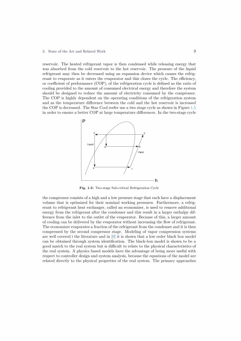
reservoir. The heated refrigerant vapor is then condensed while releasing energy thatwas absorbed from the cold reservoir to the hot reservoir. The pressure of the liquidrefrigerant may then be decreased using an expansion device which causes the refrig-erant to evaporate as it enters the evaporator and this closes the cycle. The efficiency,or coefficient of performance (COP), of the refrigeration cycle is defined as the ratio ofcooling provided to the amount of consumed electrical energy and therefore the systemshould be designed to reduce the amount of electricity consumed by the compressor.The COP is highly dependent on the operating conditions of the refrigeration systemand as the temperature difference between the cold and the hot reservoir is increasedthe COP is decreased. The Star Cool reefer use a two stage cycle as shown in Figure 1.5in order to ensure a better COP at large temperature differences. In the two-stage cycle
P
h
1
23
4
Vapor
Liquid
5 6
Fig. 1.5: Two-stage Sub-critical Refrigeration Cycle
the compressor consists of a high and a low pressure stage that each have a displacementvolume that is optimized for their nominal working pressures. Furthermore, a refrig-erant to refrigerant heat exchanger, called an economizer, is used to remove additionalenergy from the refrigerant after the condenser and this result in a larger enthalpy dif-ference from the inlet to the outlet of the evaporator. Because of this, a larger amountof cooling can be delivered by the evaporator without increasing the flow of refrigerant.The economizer evaporates a fraction of the refrigerant from the condenser and it is thencompressed by the second compressor stage. Modeling of vapor compression systemsare well covered i the literature and in [8] it is shown that a low order black box modelcan be obtained through system identification. The black-box model is shown to be agood match to the real system but is difficult to relate to the physical characteristics ofthe real system. A physics based models have the advantage of being more useful withrespect to controller design and system analysis, because the equations of the model arerelated directly to the physical properties of the real system. The primary approaches
10 Chapter 1. Introduction
for physical modeling are finite difference methods and lumped parameter methods. In[9, 10] finite difference methods are used to simulate heat exchangers with good resultsbut due to the large amount of control volumes this method results in models with avery high order, which is undesirable with respect to controller development. Lumpedparameter models results in low order models and are therefore better suited for con-troller development, and will usually also be less computationally intensive to simulate.
In the following an overview of the different modeling approaches is given.
Evaporator and CondenserThe black-box approach to modeling of heat exchangers, that was demonstrated in[8, 11] showed that the salient dynamics, which are important from a controller devel-opment perspective, are closely related to the thermal inertia of the metal in the heatexchangers. For physics based models of heat exchangers a prevalent idea is that ofthe moving boundary model, [12, 13, 14] where two or more control volumes of varyingsize is used to accurately model refrigerant properties in different phases from vapor tosub-cooled liquid. Reasonably accuracy may be obtained by a lumped parameter modelwith a moving boundary between each of the control volumes [15].
CompressorThe compressor is a determining factor for system capacity because it drives the flowof refrigerant and any error in the predicted mass flow will be propagated to the othercomponents of the system. Therefore, a compressor model with an accurate predictionof mass flow rate is essential for system level simulation, but also for control becausethe compressor model determines the important system gain from compressor speedto capacity. According to [16] there are three categories of reciprocating compressormodels; Detailed physics based dynamical models; Efficiency based models that arebased on an ideal compression and isentropic efficiency; The last category is map basedmodels which is a table lookup of performance data or a polynomial fit to the datatable. Detailed physics based models are able to reflect the dynamics for each strokeof the compressor and the heat transfers between the refrigerant and each part for thecompressor. Such models are well suited for compressor development but generally toocomputationally demanding for system level simulation. Efficiency based models assumeadiabatic compression and may include physical details [17] such as displacement andclearance volume to improve accuracy. Most compressor manufacturers supply perfor-mance data for their compressor in the form of 10 coefficient polynomials [18] that maybe used to predict the compressor performance in map based models, within limits forthe data.
Expansion valveThe most important property of an expansion valve model is the ability to accurately

3. State of the Art and Related Work 11
reflect the mass flow because it has a large impact of system capacity. An expansionvalve is basically an orifice that limits the flow of a substance which results in a pressuredrop, and this has been described well in the literature [19, 20, 21]. In [22] it is shownthat the general orifice model is accurate for expansion valves when manufacturer datais used to parametrize the expansion valve model.
EconomizerThe economizer is a plate heat exchanger, and modeling of these are described well inthe literature [23, 24] with model fidelity ranging from very detailed models that ac-curately reflects flow dynamics and distribution to simple steady state models that arebased on the logarithmic mean temperature difference (LMTD) [25].
ReceiverA receiver is a container where excess refrigerant is stored when load conditions ofthe system requires a smaller refrigerant charge than what is actually loaded into thesystem. An accurate physics based dynamic model is described in [15] where also thereceiver interaction with the condenser is described. A receiver model matched againstexperimental results is described in [26] where it is found that a lumped receiver modelis a good match to the real system, at high refrigerant charges where phase separationwas observed in the receiver.
3.3 Simulation of Refrigeration Systems
In [27] a survey of different simulation techniques for refrigeration systems is carried outand it is found that a wide range of very different techniques are used.
Energy system simulation is a mature field where tools such as TRNSYS [28], thatprovides a library of energy system components and its own system description lan-guage, have been used for more than 35 years. The Department of Energy Engineeringat Technical University of Denmark have developed WinDali [29] for simulation of re-frigeration systems where models are compiled to native machine code which make thesimulations very fast.
Dymola [30] is a relatively new tool that may be used to simulate almost any typeof dynamic system from a set of symbolic equations that describe the system behavior.The tool depends on the free Modelica [31] language, to describe the physical systemwith a high layer of abstraction. A range of classes that describes a physical propertysuch as voltage, flow or pressure, may be used for component model I/O. It is notnecessary to define the direction of signals between components when the models aredeveloped because Dymola has automatic ordering and reduction of the final set ofequations, before the simulation is run. This is very convenient for the user becauseequations may be listed in arbitrary order and arranged in the most comprehensibleway. The final set of equations may be simulated by a range of different solvers and in

12 Chapter 1. Introduction
[32] the importance of choosing the correct solver, with respect to model properties, isdemonstrated. In [26] Dymola is shown to be well suited for simulation of refrigerationsystems due to the ease of model formulation and large library of pre-defined models.
The tool that is most commonly used for controller development is MatlabR©, which
also includes state-of-the-art toolboxes for many scientific and engineering disciplines,including modeling and controller design. It has an active on-line community thatcontributes with tools and helper functions. It provides a range of solvers for solvingDAE’s, PDE’s and ODE’s and it has good integration with other languages such asC, C++ and Java which can be used as a flexible external interface. Simulink
R© is atool for creating and simulating complex models from built-in or custom blocks, whichmay be added to the Matlab
R© suite. The models may be simulated using a range ofdifferent solvers and if algebraic loops exist Simulink
R© tries to break them by insertingzero-order-holds. The solvers that are available in Simulink
R© are a set of different orderstiff and non-stiff solvers [33], and theses solvers are also available inside the standardMatlab
R© environment.According to [34] simulation of a system, that includes states that have very different
dynamical speeds, as a monolithic block has the drawback that during changing condi-tions the step size for the slow states are much smaller than what is needed to achievesatisfactory accuracy. It is shown in [34, 27] that the fast dynamical states in manycases can be converted into steady state equations, resulting in a faster simulation. An-other way of reducing the computational load is presented in [35, 36] where a multi-ratesimulator is used to simulate the fast and slow parts of a model separately which givesa substantial increase in simulation speed because an appropriate step size is used forall states. In [37] a modular multi-rate simulation environment is presented. Differentsolvers can be used for each of the components, making it possible to simulate mecha-tronics systems using original models that are made for different simulation tools. Itintroduces methods for solving algebraic loops that can occur when different numericalmodels are combined in the simulation environment. The modular approach has severaladvantages; It is faster to build a new simulation model from a library of componentsthan starting from scratch and it is also easier to maintain because the code is naturallydivided and therefore less likely to be entangled across component models. A drawbackwith the modular approach is that in order to run sub-models at different step sizesit is necessary to handle the exchange of data between component models. This maybe done by inserting zero order holds (ZOH) between the component models [35], butthis effectively introduces a delay between components, which may affect stability andaccuracy of the simulation. In a simulation, the impact of inserted ZOH’s depends onthe frequency of data exchange between components and the dynamical speed of thecomponents. When data exchange happens at a low frequency compared to componentdynamics, oscillatory behavior and possibly simulation breakdown is likely to occur. In[38, 39] different methods for handling data exchange between components are intro-duced and shown to give good results, in special cases. An iterative method for data

3. State of the Art and Related Work 13
exchange between component models, that guarantees stability, is presented in [37].Methods for numerical simulation of systems of differential equations are plentiful
and the field very diverse, in the sense that specialized solvers exist for almost anyscientific field where numerical simulation is used. In [40, 41, 42] the methods aredivided in two overall categories; Runge-Kutta methods and linear multi-step methods.A numerical solution to a set of ordinary differential equations is an approximation,and not an exact solution to the problem. Generally there is a trade off between thetime it takes to reach a solution and the accuracy of the solution, and most solvers aresupplied with an error tolerance that the local truncation error of the solution must staywithin. Runge-Kutta methods are a family of explicit and implicit methods that arevery common due to their accuracy and versatility, and solvers of this type are availablein both Matlab
R©, SimulinkR© and Dymola. Explicit methods calculate the future
state of a system from the current state only, while implicit methods solves an equationthat includes both the current and future state. Explicit methods are well suited fornon-stiff systems, and for same order methods, explicit solutions to non-stiff systems arefaster than implicit solutions. For stiff systems explicit methods may be very slow oreven unstable and in this case the use of implicit methods are required. For literatureon the exact algorithms, stability analysis and applications, see [33, 43, 44, 45].
3.4 Control of Refrigeration Systems
The reefer is a multiple-input multiple-output (MIMO) system for which applicablecontrol methods are single-input single-output (SISO) and MIMO controllers. A SISOcontroller is based on classical control theory and a very common implementation is inthe form of PID controllers [46], which are used in the majority of industrial controlsystems. The theory of design and tuning of PID controllers are described in [47]. Fornonlinear systems, PID controllers can only guarantee asymptotic stability around theoperation point that was used in the design, [48] and this can be addressed in a numberfor ways.
One method is detuning the controller to improve global robustness, but this canseverely impact performance of the controller. Gain scheduling is a method where thegains are varied according to the operating point, and in this way the impact on per-formance is reduced while global robustness is improved. Gain scheduling is frequentlyused in industrial applications and an overview of gain scheduling methods and theirapplications are given in [49]. Today the most advanced controller used in reefers isPID’s with gain scheduling to compensate for system nonlinearities. The drawbacks ofgain scheduling are that stability is only guaranteed around the design points and inorder to achieve global stability the system must be linearized in a fine mesh in termsof scheduling variables [50]. This scales poorly as the number of scheduling variables isincreased and for MIMO systems it can be very time consuming. Furthermore, the rateof change in the scheduling variables must be slow, compared to system dynamics and

14 Chapter 1. Introduction
this place fundamental limitations on the performance that may be achieved.Linear Parameter Varying (LPV) control is a method that incorporates robustness,
performance and bandwidth limitations into a unified framework [50, 51, 52] and there-fore global stability and performance can be guaranteed.
When a good model of the nonlinearity in a nonlinear system is available, feedbacklinearization may be applied in order to enable control with a linear controller [48]. Thefeedback linearization is a transformation that is inserted in the control loop, which incombination with the plant, forms a linear system that can be controlled with goodperformance using traditional linear methods.
If the nonlinear nature of the system is uncertain, control performance using feedbacklinearization may be significantly degraded. The problem of uncertainties in models anddisturbances is addressed by robust control design methods, [53] that guarantee stabilityand performance within given bounds for disturbances and system uncertainties.
Reduced Energy Consumption for ReefersIn order to increase efficiency at part load the QUEST control scheme was developedby Wageningen UR [4], resulting in a very large increase in efficiency for reefers withoutgood capacity regulation. Based on laboratory and field trials the temperature fluctu-ation limits and ventilation requirements for typical cargo such as apples and bananaswere mapped, and this knowledge was implemented into QUEST. The scheme exploitsthe temperature fluctuation limits to run the compressor in on/off operation withoutunloading or throttling, which greatly improves system efficiency. The QUEST pro-gram also reduces power consumption, by reducing the amount of ventilation, whichsaves power on the fans. All electrical power consumed by the evaporator fans ends upas heat inside the container and this heat must then be removed by the refrigerationsystem. Therefore, a reduced ventilation rate also results in lower power consumptionby the compressor. In the scientific literature the amount of work specific to reefers islimited to the studies that laid the foundation for the QUEST control scheme, which isa PhD thesis [54] and some papers [55, 56, 57, 58], that has focus on cargo quality. Theyall have good and detailed models of the cargo with respect to quality, but the refriger-ation system is not treated in detail. For reefers the QUEST scheme [4] is currently themost advanced approach but while it is based on experiences gathered through the useof Model Predictive Control (MPC) [54] to improve product quality control and reduceenergy consumption it does not adapt to external disturbances.
In [54] MPC was used to control the product quality of chilled cargo in refrigeratedcontainers with the focus on modeling and control of the cargo quality, resulting in areduction of mass loss in the cargo due to less evaporation and lower energy consumptiondue to reduced ventilation rate.
Model Predictive Control was introduced in the petro-chemical industry in order tocontrol difficult processes with long delays and unknown states but today it is used ina wide range of applications such as power plant control and the automotive industry
3. State of the Art and Related Work 15
[59]. MPC is used for optimizing control of processes with respect to known futuredemands or known future changes in external conditions, while keeping within a givenset of constraints. The performance of MPC is highly dependent on the quality of themodel on which it is based because it is used to predict the behavior of the system overthe prediction horizon without the possibility of error corrections from measurements.For nonlinear systems where the model dynamics may change, either a nonlinear oradaptive linear approach must be used in order to keep performance and avoid violat-ing constraints. The drawback of using MPC is that it is computationally heavy andtherefore not very well suited for embedded systems such as the Star Cool reefer con-troller. Methods for reducing the quadratic problem of an MPC to a simpler explicitpiece-vise linear function have however been described in the literature and in [60, 61]this is demonstrated.
In [62] MPC is used to exploit daily variations in ambient temperature by coolingmore when the COP is higher, during the night where temperature is low, using thecargo to store some cooling which reduces the amount of cooling needed during theday where the COP is lower. Another study where MPC is used for quality control is[63] where future spikes in ambient temperature, that is too large for the refrigerationsystem to handle, is countered by cooling the food in a supermarket display case inadvance. In [64] saturation of a refrigeration system due to high ambient temperatureis countered by a learning based algorithm that pre-cools the foodstuffs in the displaycases a supermarket based on previous saturations of the refrigeration system. Overtime the system "learns" when to apply extra cooling in order to counter anticipatedhigh temperatures in the future.

16 Chapter 1. Introduction
4 Project Objectives
ObjectivesThe overall objective of this project is to investigate the potential for reduced energyconsumption on the Star Cool reefer by the introduction of modern control methods,without compromising the quality of the transported goods. A model based controldesign approach is chosen because the system is well known and variations between in-dividual reefers are small. Therefore, a dynamic model of the refrigeration system thathas adequate accuracy for control design is needed. This means that the model shouldaccurately reflect the measurements that are used as controller inputs, both staticallyand dynamically.
Test and verification of control algorithms on reefers can be very expensive, especiallywhen realistic load profiles are required and the conditions inside and around the reeferneeds to be controlled accurately. This requires a test cabin that can contain a reefer,equipped with a HVAC system large enough to suppress fluctuations in air temperaturearound the reefer, while the reefer is running. Furthermore, such tests can be very timeconsuming, because of the slow dynamics of the cargo. The cost of running these testscan be reduced by simulating the reefer system, using a simulation model. It is impor-tant that the speed of simulation is significantly faster than testing on a real systemand that the results of the simulation are accurate. A simulation method that possessesthese properties must therefore be identified.
A reduction in energy consumption of the Star Cool reefer is desired and could beobtained through modern control. The available measures for reducing the energy con-sumption are the thermal inertia of the cargo that can be used as a buffer, the ventilationrate inside the container and it may also be possible to optimize control set-points. Ap-propriate control methods should therefore be investigated and a controller setup thataddress the different challenges present on a reefer, should be selected.
Commercial ScopeFor Lodam an important outcome of the project is to reduce the time it takes to de-velop, test and verify new controllers. This go hand in hand with the research objectivesfor modeling and simulation, but it also means that the simulation tool must be easyto work with and that it must have easy access to good controller development capa-bilities. Such capabilities are found in Matlab
R© and, for commercial reasons, it wasdecided that the methods developed in this study should be implemented in Matlab
R©.This has the additional advantage that a wide range of tools for data analysis and mod-eling already are available in Matlab
R© and these could be useful to the project as well.
When hardware components on the reefer are changed it may require that the model is

4. Project Objectives 17
changed as well in order to reflect the dynamics of the new hardware and this shouldbe easy. Therefore, it is required that the simulation method is flexible with respect todifferent hardware configurations.
A controller that reduces energy consumption, through the use of the thermal iner-tia of the cargo, requires optimization over a long period which can be computationallyheavy and this does not fit well with an eventual implementation in the embedded con-troller of the Star Cool reefer. Therefore, methods that reduce the computational loadof the controller should be investigated.
The objectives can be summarized as below:
• Objective I: Control modelTo create a non-linear dynamical model of the reefer that is suitable for devel-opment of controllers. The model should be accurate to within 1 Kelvin on themeasurements that are important for control, and this must be verified againstdata from a real system.
• Objective II: Simulation modelTo investigate if it is possible to formulate a non-linear dynamical model suchthat it can also be used for test and verification of controllers through simulation.The simulation model is required to have an accuracy such that controllers canbe tested on the model and subsequently used on the real system without furthertuning. Furthermore, it is required that the model is able to simulate a period of21 days, which corresponds to a normal trip of a container.
• Objective III: Simulation methodTo investigate appropriate methods that enables simulation of the non-linear modelwith emphasis on accuracy and simulation speed. The speed should be at least anorder of magnitude faster than real time and the error introduced by the simulationshould not exceed the variance in system tolerances on the reefers in the field.
• Objective IV: Reduced energy consumptionInvestigate the potential for reducing energy consumption during transport of frozencargo in reefer containers, by using the thermal inertia of the cargo as a buffer,and by reducing the ventilation rate.
The work presented in this thesis can be related to one or more of the above objectives.
18 Chapter 1. Introduction
5 Summary of Contributions
The main contributions in this project are listed in this section and divided into threeparts.
5.1 Reefer Model
Proposal for a control oriented nonlinear dynamical model of a reefer container thatis verified against data from a real container at multiple capacity set-points with anerror of less than 1K on the states important for control. The model is an extensionof the ideas presented in [11] where it is shown that, for a car air conditioning system,a model that includes the dynamics of the metal in the heat exchangers and steady-state equations for the refrigerant control volumes has adequate accuracy to be usedfor controller design. The proposed model is a collection of components, which havebeen found in the literature and adapted, that together form an accurate representationof the Star Cool reefer. It has been shown that accuracy of the presented model isadequate for controller design and therefore the ideas presented by [11] also holds forthe more complex reefer refrigeration system. A description of the development, test andverification of the model can be found in and the equations for the model are presentedin [Paper C Section 2].
The model is currently being used by Lodam for development, test and verificationof control and fault detection algorithms and it has proved to be a valuable tool thatsignificantly reduces development time.
5.2 Simulation
A proposal for an efficient and accurate simulation method for the nonlinear model ofthe refrigeration container. An analysis of solver choice demonstrates that, for modularsimulation, using a simple solver can be faster than more advanced solvers, withoutsacrificing accuracy. The simulation tool provides a solid and necessary base for devel-opment and test of model based controllers.
The contributions from this work related to the commercial interests are the sim-ulation environment and its associated tools which will enable Lodam to improve andspeed up the efforts for model based controller development for the Star Cool reefer.
The modular multi-rate simulation of the reefer is presented in [Paper A Section 3]and the comparison of methods and solvers is presented in [Paper B Section 2].
5.3 Adaptive Model Predictive Control for a Reefer
Proposal for an adaptive controller strategy that is able to reduce the energy con-sumption of the reefer with up to 21% by exploitation of daily variations in ambient

5. Summary of Contributions 19
temperature and a reduction of the rate of ventilation such that it matches the actualdemand. A cargo estimator is used to estimate important unknown states and cargoparameters that are used to continuously update the linear model for the MPC, whichallows the controller to adapt to cargo with different dynamics and heat transfer rates.A series of optimizations on the MPC reduces the computational load and makes itcommercially interesting. The control strategy is presented in [Paper D Section 2.3].

20 Chapter 1. Introduction

Chapter 2
Summary of Work
In this chapter the contributions from the project are described in detail. The descriptionis divided in three sections concerning modeling, simulation and control of the reefer,respectively. The details of the reefer model are described in Section 1, the reefersimulation tools and experiments are described in Section 2 and the proposed adaptivecontroller for the reefer is described in Section 3.
1 Reefer Container Modeling
This section describes the important characteristics of the reefer system and summarizesthe most important aspects of the work on the reefer simulation model. The equationsof the model are described in detail in [Paper C].
1.1 Objectives
Development, test and verification of model based controllers require a good systemmodel and therefore a large effort has been put into the development and verificationof a simulation model for the reefer container. In order to meet the objectives of theproject the model must be a good match to the dynamics of the refrigeration system,in order to support the development of a controller that is able to keep the systemclose to the energy optimal set-points. The model must also match the steady-stateproperties of the real system closely, in order to support development of controllers forlong term energy optimization. The model should be designed such that it can serve asa tool for future development and test of controllers in order to meet Lodam’s ambitionof reducing the development time of new controllers. This requires that the model isflexible and that it can be reconfigured for other tasks if needed. One such task could
21

22 Chapter 2. Summary of Work
be simulation of faults such as lack of refrigerant or reduced compressor capacity dueto a mechanical fault and therefore the model must include the refrigerant circuit.
1.2 Control Oriented Modeling
Creating a model that meet the objectives requires identification of the system char-acteristics that impacts energy efficiency and for refrigeration systems this has beeninvestigated in a range of different works. In [65] a simple refrigeration system withvariable speed fans and compressors are analyzed with the conclusion that the relativespeed of the compressor and the fans are very important for the overall power consump-tion of the system. This means that the model at least should be able to accuratelyreflect the mass flow through the compressor, the condensing pressure and the suctionpressure, in dynamic and steady state conditions. The superheat of the evaporator isalso an important parameter, because it has a big impact on the energy efficiency ofthe system, and therefore the dynamics and steady state properties of this parametershould also be matched by the model.
A simple way to achieve a good match on these parameter dynamics are presentedin [11] where the authors show that the salient dynamics of a refrigeration system isdetermined by the thermal time constants of the metal in the heat exchangers andthis observation is a major inspiration for the development of the model presentedhere. Achieving a good match of steady state conditions for a refrigeration systemwhere the range of operation is as large as it is on the reefer is challenging because thecapacity of the system changes with the difference between the ambient temperatureand the temperature inside the container. This effect is caused by the fact that thesaturated suction temperature, T0, must be lower than the air inside the container inorder to cool the air and due to a reduction in compressor efficiency at higher differentialpressure. Both effects are related to non-linear refrigerant characteristics and thereforethe refrigerant circuit in the model should match these characteristics. One way toachieve this is to make a first principles model of the full system that accurately modelsthe state of the refrigerant in all control volumes, but this requires a lot of work andwould yield a model that was more advanced than needed, so a simpler approach waspursued. The interesting dynamics from a control perspective is covered by modelingthe thermal time constants of the heat exchangers metal and therefore it was found thatthe approach presented in [66], where the refrigeration circuit is modeled by steady stateequations, could be used. So to summarize, the model presented here use first principlessteady state equations for the refrigerant circuit and first principles dynamical equationsfor the larger thermal capacities in the system, such as the metal in the heat exchangers,the air in the container and the cargo. First principles are substituted by assumptionswhere it reduces model complexity and has a small effect on model accuracy. If it isfound at a later point in time, that the component models that have been selectedfor the system model are inadequate with respect to accuracy, the modular modeling
1. Reefer Container Modeling 23
approach ensures that components can be easily substituted with better alternativesfrom the literature.
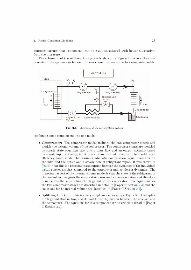
The schematic of the refrigeration system is shown on Figure 2.1 where the com-ponents of the system can be seen. It was chosen to create the following sub-models,
Fig. 2.1: Schematic of the refrigeration system
combining some components into one model:
• Compressor: The compressor model includes the two compressor stages andmodels the internal volume of the compressor. The compressor stages are modeledby steady state equations that give a mass flow and an output enthalpy basedon speed, input enthalpy, input pressure and output pressure. The model is anefficiency based model that assumes adiabatic compression, equal mass flow onthe inlet and the outlet and a steady flow of refrigerant vapor. It was shown in[66, 67] that this is a reasonable assumption because the dynamics of the individualpiston strokes are fast compared to the evaporator and condenser dynamics. Theimportant aspect of the internal volume model is that the state of the refrigerant inthe control volume gives the evaporation pressure for the economizer and thereforeit influences the sub-cooling of refrigerant to the evaporator. The equations forthe two compressor stages are described in detail in [Paper C Section 2.3] and theequations for he internal volume are described in [Paper C Section 2.1].
• Splitting Junction: This is a very simple model for a pipe T-junction that splitsa refrigerant flow in two, and it models the T-junction between the receiver andthe economizer. The equations for this component are described in detail in [PaperC Section 2.2].

24 Chapter 2. Summary of Work
• Condenser: This component removes energy from the refrigerant that exits sec-ond stage of the compressor, thereby condensing it into a liquid. It was attemptedto use a simple model for the condenser with only one control volume and a roughassumption for the pressure drop due to flow resistance, making the input pres-sure at the compressor equal to the pressure in the receiver plus a variable deltapressure that depends on the mass flow. The equations and assumptions for thecondenser are described in detail in [Paper C Section 2.4].
• Receiver: The receiver is a buffer tank for excess refrigerant that is not currentlylocated in other components. It is needed because the amount of refrigerant re-quired for the evaporator and condenser to run efficiently varies with temperatureand load. The receiver has two control volumes; One for the liquid refrigerant andone for the refrigerant vapor where the state of the vapor determines the pressure.In [Paper C Section 2.5] the equations and assumptions of the receiver is explainedin detail.
• Economizer with Expansion Valve: The economizer is a counterflow plateheat exchanger that has evaporating refrigerant on the cold side and liquid refrig-erant on the hot side. It sub-cools the refrigerant going to the evaporator and ithelps boost system performance by increasing the refrigeration systems efficiencyand capacity. The thermal time constant of the metal in the economizer is smalland therefore it is not modeled for this component. Instead, it models the steadystate heat transfer from the liquid refrigerant to the evaporating refrigerant withone control volume for each side, using a logarithmic mean temperature difference(LMTD). The expansion valve for the economizer is included in this model becauseit is a simple steady state calculation of mass flow from the pressure differenceover the valve and the density of the liquid that enters the valve. The equationsof the economizer are available in [Paper C Section 2.7] and the equations andassumptions for the expansion valve are described in [Paper C Section 2.6].
• Evaporator with Expansion Valve: Controlling the evaporator is often themost difficult part of refrigeration system control due to the highly nonlinearbehavior of the superheat when it approaches zero where the sensitivity of themeasurement vanishes. The superheat is the difference between the saturatedsuction temperature and the actual suction temperature and it is a measure forexcess energy added to the refrigerant vapor after full evaporation. A highersuperheat is achieved by lowering the pressure, but this reduces the efficiency ofthe compressor so the theoretical optimal point of operation is a superheat of zerokelvin. It is important that the refrigerant reaching the compressor is dry becauseliquid refrigerant can wash away the oil film that protects the pistons againstwear and tear. When the superheat is zero the system is very close to liquidslugging, where the refrigerant is no longer completely dry. If liquid slugging

1. Reefer Container Modeling 25
occurs the superheat cannot be measured because the sensitivity of the superheatmeasurement has dropped to zero. Therefore, the normal approach is to run witha superheat that is as small as possible, and if a superheat controller is to bedesigned from the model it is required that the accuracy of the modeled pressureand suction temperature is high. This is achieved by modeling the evaporatoras two control volumes separated by a moving boundary that depends on theamount of liquid refrigerant in the evaporator. In the first control volume therefrigerant evaporates and in the second it is superheated which means that thesuperheat depends on the position of the boundary, or the filling of the evaporator.As for the economizer, the expansion valve model is included in the evaporatormodel. The equations of the evaporator are available in [Paper C Section 2.8] andthe equations and assumptions for the expansion valve are described in [Paper CSection 2.6].
• Container and Cargo: The container and the cargo are the largest thermalcapacitances of the system and the temperature of the return air from the containeris closely tied to the temperatures in the container. The cargo hold is modeled astwo lumped volumes, one is the cargo and the other is the aluminum floor whichis the main mass of metal inside the container. It is assumed that the air passingover the floor has the supply air temperature and that the temperature of the airpassing over the cargo is the average of the supply and return temperatures. Thecargo in the model that is used in this thesis is a load of frozen pork meat thatwas kindly provided by MCI for modeling experiments, which led to estimatesof the heat transfer coefficient from the air to the cargo. In these experimentsthe mass and type of the cargo was known, making it easy to estimate the heattransfer coefficient but normally this is not knowledge that the controller has andthat presents a challenge that must be overcome if a model based controller thatincludes the cargo dynamics is to be used. A temperature measurement of thecargo is not always available and this complicates the estimation of cargo dynamicsfurther. This issue is treated is Section 3.3. The equations for the model of thecargo and the cargo hold are described in [Paper C Section 2.9]
The structure of the reefer model is defined by the collection of sub-models which havebeen refined and adapted to the current needs during the project.
1.3 Identification of Model Parameters
The structure is an important part of achieving good model performance but anothervery important part is the model parameters which were identified from measurementsfrom the reefer in different operating points. The important parameters for this modelare the heat transfer coefficients and the parameters that influence the mass flow of thecompressor stages and expansion valves.

26 Chapter 2. Summary of Work
The mass flows are important to get right because they define the amount of re-frigeration that is achieved from a given set of control values and they were calibratedfrom direct mass flow measurements on the reefer in different operating points. For thecompressor model the adjustment were done by adapting the valve loss such that themass flow at low suction pressure were correct. The expansion valve model was adaptedby adjusting the characteristic constant.
The heat transfer coefficients were initially calculated from the cooling capacity andrelevant steady state temperatures at different operating points, but due to inaccuraciesin the model assumptions some subsequent minor adjustments was needed for the bestresult. The heat transfer coefficients influence the dynamics because they are determin-ing for the amount of energy transferred between the main thermal capacitances thatmodels the system dynamics and the adjustments done to the heat transfer coefficientswere aimed at getting a better match of the system dynamics.
1.4 Verification and Results
In this section the verification of the full system and the component models is described.The requirements for the model that was described in Section 4, states that the modelmust be accurate to within 1K on the measurements that are used for control, in orderto be suitable for development of controllers. The objective for the simulation modelrequires an accuracy that would allow most of the development of a controller to be doneon the model, with only verification done on the real system. A controller developedfor a fleet of reefers must be designed to be robust against the variations in dynamicalresponse and capacity that exists from unit to unit. This means that the error of themodel should be smaller than the error caused by variation between reefers in the field.Accurately measuring what the error is on reefers in the field is difficult but it was judgedto be significantly larger than what is required for the control model. Therefore, bothmodels may be verified by checking that the error on measurements that are importantfor control is below 1K in steady state and dynamic situations. The measurements,that are normally used by the reefer controller, are the supply air temperature Tsup,the return air temperature Tret, the suction temperature Tsuc, the saturated suctiontemperature T0 and the saturated discharge temperature TC . The cooling capacity maybe calculated from the evaporator fan speed and the difference between Tsup and Tret,and this can be used to verify that the cooling capacity of the model match the realsystem. This is significant because a matching cooling capacity indicates that the staticproperties of the compressor and the expansion valve are accurate.
A reefer with a cargo of frozen pork meat was kindly made available for the testby MCI and verification of the system model performance was done by comparing themeasurements relevant for control, from an open loop simulation on the model and datarecorded from a reefer. The open loop simulation were driven with the control signalsrecorded from the reefer.
1. Reefer Container Modeling 27
0
20
40
FcprVexpVecoFcondFevap
0
1000
2000
3000
Coo
ling
Cap
[W]
QCool measQCool model
10
15
20
Tc
[°C
]
Tc measTc modelTamb
−24
−22
−20
Tsu
p, T
ret [
°C]
Tsup measTsup modelTret measTret modelTcargo measTcargo model
0 20 40 60 80 100 120 140 160 180
−24
−22
−20
Time [min]
Tsu
c, T
0 [°
C]
Tsuc measTsuc modelT0 measT0 model
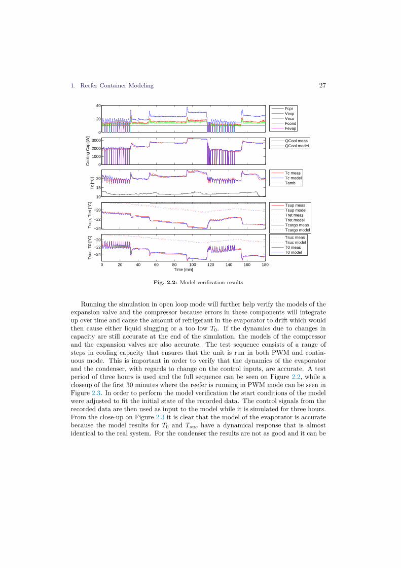
Fig. 2.2: Model verification results
Running the simulation in open loop mode will further help verify the models of theexpansion valve and the compressor because errors in these components will integrateup over time and cause the amount of refrigerant in the evaporator to drift which wouldthen cause either liquid slugging or a too low T0. If the dynamics due to changes incapacity are still accurate at the end of the simulation, the models of the compressorand the expansion valves are also accurate. The test sequence consists of a range ofsteps in cooling capacity that ensures that the unit is run in both PWM and contin-uous mode. This is important in order to verify that the dynamics of the evaporatorand the condenser, with regards to change on the control inputs, are accurate. A testperiod of three hours is used and the full sequence can be seen on Figure 2.2, while acloseup of the first 30 minutes where the reefer is running in PWM mode can be seen inFigure 2.3. In order to perform the model verification the start conditions of the modelwere adjusted to fit the initial state of the recorded data. The control signals from therecorded data are then used as input to the model while it is simulated for three hours.From the close-up on Figure 2.3 it is clear that the model of the evaporator is accuratebecause the model results for T0 and Tsuc have a dynamical response that is almostidentical to the real system. For the condenser the results are not as good and it can be

28 Chapter 2. Summary of Work
0
10
20
30
FcprVexpVecoFcondFevap
0
1000
2000
3000
Coo
ling
Cap
[W]
QCool measQCool model
10
15
20
Tc
[°C
]
Tc measTc modelTamb
−24
−22
−20
Tsu
p, T
ret [
°C]
Tsup measTsup modelTret measTret modelTcargo measTcargo model
0 5 10 15 20 25 30
−24
−22
−20
Time [min]
Tsu
c, T
0 [°
C]
Tsuc measTsuc modelT0 measT0 model
Fig. 2.3: Close-up of the start/stop phase
seen that the error on Tc exceeds 1K 10 minutes in to the simulation. Furthermore, thedynamics on start of the compressor cause a small pressure spike just after start wherethe model have a more soft pressure increase. This indicates that some dynamics maybe missing, and considering the simple model used for the condenser, this is entirelypossible. It seems that the condenser model lacks sensitivity to changes in ambient tem-perature, which is especially clear in the end where there is a sudden drop in ambienttemperature. The cooling capacity matches very well throughout the simulation andthis indicates that the steady state properties of the model are excellent. The supplyand return air temperatures show a good match to the reefer but there seems to be asmall phase shift on Tsup, which could be caused by missing sensor dynamics.
Verification of component performanceIn the following the performance of the individual component models are rated, basedon observations from the open loop test.
• Compressor: The compressor is deemed to be very accurate because the coolingcapacity of the system and the model are accurate to within ±100W for the

1. Reefer Container Modeling 29
majority of the test time. A set of measurements of refrigerant flow through theevaporator in steady state were provided by MCI and the results in Figure 2.4demonstrates that the model of the compressor is reasonably accurate over thefull range in speed and suction pressure. The flow was measured over in theliquid line, just before the evaporator expansion valve, and due to the pulsatingmodulation of the expansion valve the measurements vary, especially at high flowwhere the flow-meters internal averaging of the flow were challenged the most.
• Condenser and Receiver: Verification of the receiver and condenser modelsare difficult because the only available measurement is Tc, but it can be seenthat the steady state pressure level is reasonably accurate but also that some fastdynamics are missing. The steady state pressure determines the enthalpy on therefrigerant that is forwarded to the economizer and drives the mass flow throughthe expansion valves. Therefore, when the steady state pressure is accurate, theimpact of the errors on the fast dynamics is seen as limited.
• Economizer with Expansion Valve: The economizer on the Star Cool unitare normally controlled in open loop and therefore there are no measurementsavailable for direct verification of the economizer model. Verification of the steadystate properties of the economizer must therefore be done through observations onthe full system. The refrigerant entering the economizer is on the bubble point atthe discharge pressure and the enthalpy is then lowered through sub-cooling of therefrigerant by the economizer. The amount of sub-cooling have a direct impacton the cooling capacity provided by the evaporator, which can be measured andhave been verified to closely match the real system. Because the compressor massflow is accurate, it can be deduced from the energy balance of the evaporator thatte economizer model provides the correct amount of sub-cooling.
• Evaporator with Expansion Valve: The evaporator model includes the follow-ing important states: Tsup, Tsuc and T0, which are all measured and therefore canbe verified directly. The results on Figure 2.2 show that the static and dynamicresponse of the evaporator model closely match the real system. Verification ofthe expansion valve is done against the flow measurements shown on Figure 2.4,from which it can be concluded that the accuracy of the expansion valve model isadequate.
• Container and Cargo: The model of the container cargo-hold and the cargomodels a single state, Tret, with slow dynamics that depends on the thermal inertiaof the cargo and some faster dynamics from the thermal inertia of the cargo hold.Verification of the slow dynamics are difficult from only three hours of simulation,but due to their dependency of the nature of the cargo the slow dynamics areexpected to vary in the field and therefore an accurate model less important.An accurate model of the fast dynamics are however important because they are
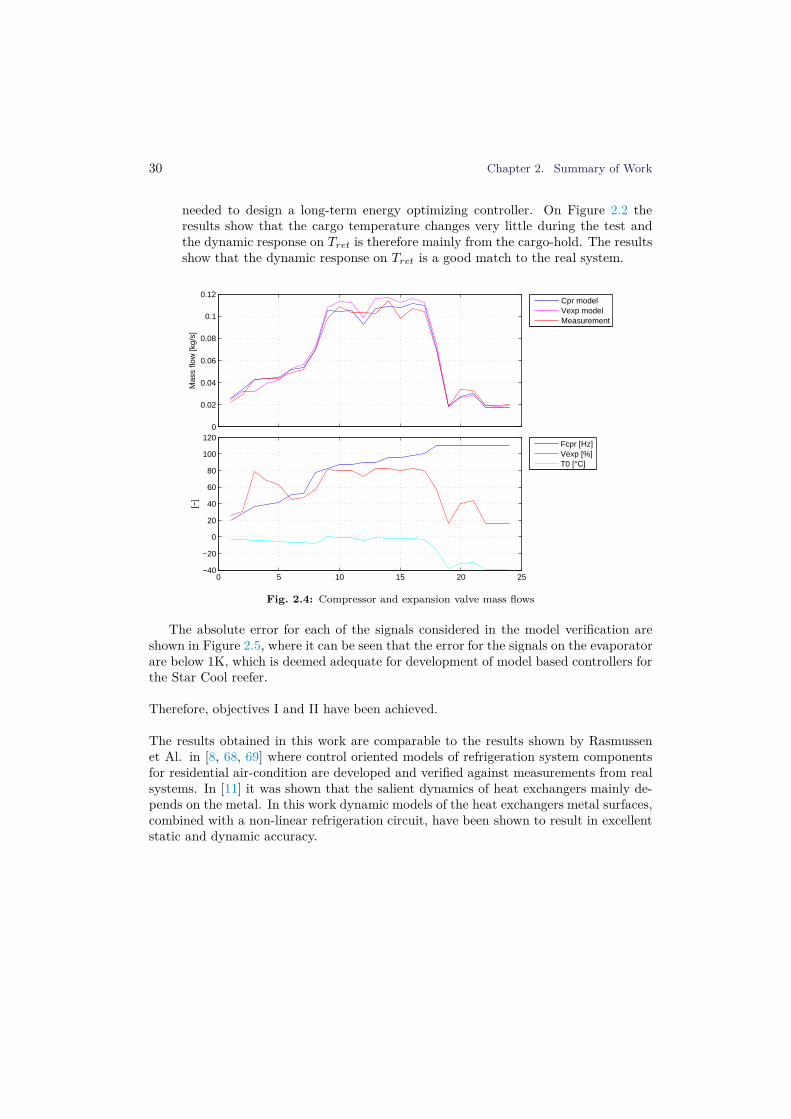
30 Chapter 2. Summary of Work
needed to design a long-term energy optimizing controller. On Figure 2.2 theresults show that the cargo temperature changes very little during the test andthe dynamic response on Tret is therefore mainly from the cargo-hold. The resultsshow that the dynamic response on Tret is a good match to the real system.
0
0.02
0.04
0.06
0.08
0.1
0.12
Mas
s flo
w [k
g/s]
Cpr modelVexp modelMeasurement
0 5 10 15 20 25−40
−20
0
20
40
60
80
100
120
[−]
Fcpr [Hz]Vexp [%]T0 [°C]
Fig. 2.4: Compressor and expansion valve mass flows
The absolute error for each of the signals considered in the model verification areshown in Figure 2.5, where it can be seen that the error for the signals on the evaporatorare below 1K, which is deemed adequate for development of model based controllers forthe Star Cool reefer.
Therefore, objectives I and II have been achieved.
The results obtained in this work are comparable to the results shown by Rasmussenet Al. in [8, 68, 69] where control oriented models of refrigeration system componentsfor residential air-condition are developed and verified against measurements from realsystems. In [11] it was shown that the salient dynamics of heat exchangers mainly de-pends on the metal. In this work dynamic models of the heat exchangers metal surfaces,combined with a non-linear refrigeration circuit, have been shown to result in excellentstatic and dynamic accuracy.

1. Reefer Container Modeling 31
−3 −2 −1 0 1 2 30
10
20
30Temperature Error Distribution
Error [K]
Fre
quen
cy [%
]
TcTsupTretTsucT0
−400 −300 −200 −100 0 100 200 300 4000
5
10Cooling Capacity Error Distribution
Error [W]
Fre
quen
cy [%
]
Fig. 2.5: Model error distribution
1.5 Contributions
The contribution from this part of the work is a proposal for control oriented model of aStar Cool reefer container, that verifies that the methods for control oriented modelingof refrigeration systems in car air conditioners presented in [11] also holds for morecomplex systems. The proposed model is a collection of components, which have beenfound in the literature and adapted, that together form an accurate representation ofthe Star Cool reefer.
The model is currently being used by Lodam for development, test and verificationof control and fault detection algorithms and it has proved to be a valuable tool thatsignificantly reduces development time. It enables the development of model basedcontrollers that are capable of reaching the set-point faster and have better disturbancerejection than existing controllers. The modular nature of the model and the integrationwith Matlab
R© have proved to be valuable every time the model have needed to bechanged or updated to meet the demands of different development tasks.
32 Chapter 2. Summary of Work
2 Simulation
This section describes the investigations into different simulation methods for the reefermodel described in [Paper C] which was supported by the simulation environment andassociated tools that are described in [Paper A] and [Paper B]. Modular and monolithicsimulation methods are evaluated and compared with respect to speed and accuracy,using Matlab
R©’s built in ode15s solver and a simple Variable Step Forward Euler(VS-FE) solver. This reveals that for the reefer model, the VS-FE solver is significantlyfaster than ode15s solver, while keeping the same accuracy.
2.1 Objectives
The work carried out with respect to simulation was initially aimed at achieving thecommercial goal of enabling Lodam to develop cutting edge control for the Star Coolreefer and improve the time to market. This required a way to simulate the reefer modeland a way to use the model as a basis for development of controllers in an automatedway, in order to speed up the development process and it was found that the best optionfor controller development was by utilizing Matlab
R©’s control toolbox. The resultingobjective was to make it possible to simulate a modular model of the reefer analogous toWinDali [29] or TRNSYS [28], but inside Matlab
R©, in order to achieve synergy withMatlab
R©’s controller development tools. This resulted in the simulation environmentdescribed in [Paper A], where it was found that there was a theoretical increase insimulation speed, when simulating the model in a modular configuration, using themulti-rate method, instead of simulating the model as a monolithic block. This resultedin the scientific objective of investigating the theoretical increase in simulation speedand this work is described in [Paper B].
2.2 Simulation Environment
The most important item among the modeling tools is the simulation environmentthat consists of a model loader and a range of different simulation functions that cansimulate the model in monolithic or modular configurations. The model loader parsemodel definitions written in Extensible Markup Language (XML) and verify the integrityof the connections between component models. Built into the simulation functions areprofilers that allow the user to retrieve and plot information on the simulation time andthe number of steps required for each of the component models, after a simulation hasbeen completed. The essential features and results for these tools are described in thefollowing.

2. Simulation 33
Model Loader and Simulation Model Description Language
The simulation model for the reefer consists of a collection of component models whereeach model consists of an m file containing the input/output equations, an XML file de-scribing the input/output properties of the model, its execution mode, and the nameof the corresponding m file. The interface of the m file is compatible with the solvers ofMatlab
R©’s ODE suite [33] and have the form x = f(x, u, t, p) such that they may besimulated using all of Matlab
R©’s built-in solvers [70]. In the XML file it can be specifiedwhich solver to use, allowing each component to be simulated by the solver best suitedfor the job. A similar approach was demonstrated for electro mechanical systems in [36]and [37] where a system is divided into sub systems by their time constants and simu-lated with a solver and step size that is appropriate for each sub system. The syntaxfor writing the component model definition XML file is shown in Listing 2.1.

34 Chapter 2. Summary of Work
Listing 2.1: Component Model Syntax
<?xml version="1.0" encoding="UTF-8"?>
<component name=["Component Name]">
<inputs>
<input name=["Input1 Name"] type=["Input1 Type"] description=["Input1 Description"]/>
.
.
<input name=["InputN Name"] type=["InputN Type"] description=["InputN Description"]/>
</inputs>
<states>
<state name=["State1 Name"] type=["State1 Type"] default=["State1 Start Value"]
description=["State1 Description"]/>
.
.
<state name=["StateN Name"] type=["StateN Type"] default=["StateN Start Value"]
description=["StateN Description"]/>
</states>
<connectors>
<connector type=["type"] conid=["Conn. Name"] >
<{input, state} name=["Name"] type="Physical Entity"/>
<{input, state} name=["Name"] type="Physical Entity"/>
</connector>
.
.
</connectors>
<control_inputs>
<input name=["Input Name"] type=["Input Type"] description=["Input Description"]/>
.
.
</control_inputs>
<simulation method={"ode15s", "call"} call=[".m File Function Name"]/>
<filename>[.m File Name]</filename>
</component>
The <inputs> section contains a list of the inputs to the component model, and theinputs must be listed in the same order as they occur in the input vector of the modelfunction in the m file. Each input has a name, a type used for type-checking when inputsare connected, and a description. The <states> section is similar to the input sectionbut it describes the states of the function and a default value must be declared foreach state. The default values are used as the initial value for the states in simulationsenvironment, but it is also possible to use a custom set of initial values if needed.
The inputs of each sub component must be connected to a state in another compo-nent and this is done in the XML file that defines the structure of the simulation model,

2. Simulation 35
shown in Listing 2.2.
Listing 2.2: Simulation Model Syntax
<?xml version="1.0" encoding="UTF-8"?>
<simulation_model name=["Simulation Model Name"]>
<component_path>[Component Library Path]
</component_path>
<components>
<component name=["Component Model Name"] file=["Component Model XML File Name"]/>
.
.
<component name=["Component Model Name"] file=["Component Model XML File Name"]/>
</components>
<connections>
<connector name=["Connector Name"]>
<component name=["Component Name"] conid=["Connection Name"]/>
<component name=["Component Name"] conid=["Connection Name"]/>
</connector>
<connection name=["Connection Name"]>
<component name=["Component Name"] type="Input" input=["Input Name"]/>
<component name=["Component Name"] type="Output" output=["Output Name"]/>
</connection>
</connections>
</simulation_model>
For refrigeration systems the number of connections needed to connect the componentmodels are large. Each refrigerant pipe requires three states; Pressure, enthalpy andmass flow and in order to avoid making a connection for three states on every pipein the simulation model definition signals may be grouped together in connectors inthe component model definitions. They allow the user to connect a set of signals fromone component model to a similar set on another component model in one operation.Type checking is performed by the model loader such that signals of the same typeare connected and such that inputs always are connected to states. If the user tries toconnect two incompatible connectors the model loader returns an error and a descriptionof the nature of the problem.
During simulation a global state vector X is used to store the collection of statesfrom the component models and the model loader creates mapping matrices for each ofthe component models that maps its state and input vectors to the global state vector.The advantage of this approach is that matrix multiplications are very fast in Matlab
R©
and therefore the exchange of information between the component models are fast andefficient during simulation which keeps the overhead low. The matrix Zk maps from X
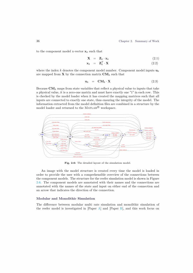
36 Chapter 2. Summary of Work
to the component model x-vector xk such that
X = Zk · xk (2.1)
xk = ZTk · X (2.2)
where the index k denotes the component model number. Component model inputs uk
are mapped from X by the connection matrix CMk such that
uk = CMk · X (2.3)
Because CMk maps from state variables that reflect a physical value to inputs that takea physical value, it is a zero-one matrix and must have exactly one "1" in each row. Thisis checked by the model loader when it has created the mapping matrices such that allinputs are connected to exactly one state, thus ensuring the integrity of the model. Theinformation extracted from the model definition files are combined in a structure by themodel loader and returned to the Matlab
R© workspace.
evap
boxTsup->Tsup
ctrl
pout->evap_psuc
hout->evap_hsuc
Tsup->Tsup
cpr
pout->pin
hout->hin_suc
econ
mdotin->mdotout1
Tret->Tret Tret->Tret
Talu->Talu
Tcargo->Tcargo
evap_vexp->Vexp
Tamb->Tamb
vfan_evap->vfan
Hevap->Hevap
Tamb->Tamb
vfan_evap->vfan
QHeat->QHeat
cpr_speed->cpr_speed
econ_vexp->Vexp
condTamb->Tamb
vfan_cond->vfan
recv
Tamb->Tamb
mdotin_suc->mdotout
hout->hdis
pim->econ_psuc
Tfc->Tfc
pim->pout2hout->hin
mdotout->mdotin
pout1->pin
hout1->hin
hout2->econ_hsuc
hout2->hin_im
mdotout2->mdotin_im
sj
mdotin1->mdotout1
mdotin2->mdotout2
pin->pdis pin->pout
mdotout->mdotin
h->hin
p->pout p->pin
hout->hin
pout1->pin1
hout1->hin1
pout2->pin2
hout2->hin2
mdotin->mdotout
Fig. 2.6: The detailed layout of the simulation model.
An image with the model structure is created every time the model is loaded inorder to provide the user with a comprehensible overview of the connections betweenthe component models. The structure for the reefer simulation model is shown in Figure2.6. The component models are annotated with their names and the connections areannotated with the names of the state and input on either end of the connection andan arrow that indicates the direction of the connection.
Modular and Monolithic Simulation
The difference between modular multi rate simulation and monolithic simulation ofthe reefer model is investigated in [Paper A] and [Paper B], and this work focus on

2. Simulation 37
the difference in speed and accuracy of the two methods. This research is enabledby a monolithic wrapper function that combines the output of the component modelfunctions into on large output vector, using the mapping matrices in the model. Theinterface of the wrapper has the same form as the component models and is compatiblewith standard ODE solvers such that it can be simulated by a solver.
Fig. 2.7: The monolithic wrapper.
Each time the monolithic wrapper function is called, it iterates through the list ofcomponent models and calls each of them with their respective input and state vectors.The outputs are then combined in the global state gradient vector X and returned tothe solver. This means that the model can be simulated as a monolithic block withoutchanging the model definition or rewriting the model equations and that ensures that atrue comparison between the two methods can be achieved. Figure 2.7 shows a diagramof how the monolithic wrapper encapsulates the component models and handles theconnections between them.
The model may also be simulated as a modular system, using the multi rate method,where the component models are simulated individually by a numerical solver overa fixed period after which the global state vector is updated. This corresponds toinserting zero order holds between the component models as shown on Figure 2.8, butthe advantage is that each component can be simulated using a solver and a step size thatis just right for that particular component. In a system where there is a large differencebetween the time constants in the component models, significant increases in simulationspeed can be achieved because slower components do not have to be simulated with an

38 Chapter 2. Summary of Work
Fig. 2.8: .
unnecessarily small step size, which reduces the computational load. The drawback ofthe approach is that the zero order holds introduces abrupt changes on the inputs tothe component models, which results in larger gradients on the states that requires asmaller step size in the simulation in order to achieve the necessary accuracy. This canbe remedied by using a higher order extrapolation algorithm than the zero order holdthat is currently used but this can result in numerical instability for tightly coupled fastand slow component models [35].
This means that there exists a trade-off between accuracy, stability and speed thatmust be considered when applying the multi-rate method. An example of the impactof inserting ZOH’s in series with the component models is shown on Figure 2.9 wherethe frequency responses of a simple linear system has been augmented with varyingdelays. The delay very significantly reduce the gain margin of the system close to thefrequency D
2 where the delay alone have decreased the phase by 180◦. Consequently, it
is necessary to ensure that the systems gain crossover frequency is lower than D2 by a
safe margin, in order to ensure stability, but also to ensure that the impact on accuracyis low. Theoretical analysis of the problems regarding optimal selection of the dataexchange rate in modular simulation can be found in the literature [71, 36, 35], butfor the reefer model it has not been necessary to apply advanced analysis, because thedynamics of the system are slow compared to the data exchange rate. This means thatit is probable, that the simulation speed can be increased through the application ofmore advanced data exchange scheduling, but that is outside the scope of this project.
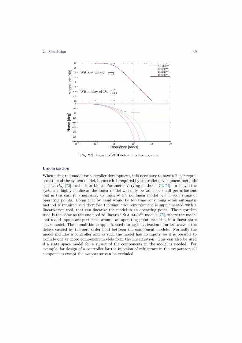
2. Simulation 39
−20
−15
−10
−5
0
5
10
15
20
Mag
nitu
de [d
B]
Without delay: 1s+0.1
With delay of Ds: e−D·s
s+0.1
10−3
10−2
10−1
100
101
102
−360
−315
−270
−225
−180
−135
−90
−45
0
Pha
se [d
eg]
Frequency [rad/s]
No delay1s delay2s delay4s delay
Fig. 2.9: Impact of ZOH delays on a linear system.
Linearization
When using the model for controller development, it is necessary to have a linear repre-sentation of the system model, because it is required by controller development methodssuch as H∞ [72] methods or Linear Parameter Varying methods [73, 74]. In fact, if thesystem is highly nonlinear the linear model will only be valid for small perturbationsand in this case it is necessary to linearize the nonlinear model over a wide range ofoperating points. Doing that by hand would be too time consuming so an automaticmethod is required and therefore the simulation environment is supplemented with alinearization tool, that can linearize the model in an operating point. The algorithmused is the same as the one used to linearize Simulink
R© models [75], where the modelstates and inputs are perturbed around an operating point, resulting in a linear statespace model. The monolithic wrapper is used during linearization in order to avoid thedelays caused by the zero order hold between the component models. Normally themodel includes a controller and as such the model has no inputs, so it is possible toexclude one or more component models from the linearization. This can also be usedif a state space model for a subset of the components in the model is needed. Forexample, for design of a controller for the injection of refrigerant in the evaporator, allcomponents except the evaporator can be excluded.

40 Chapter 2. Summary of Work
VS-FE Solver
During the work on modular and monolithic simulation of the model it was discoveredthat the ode15s solver has a significant startup overhead which impacted the resultsin modular simulations where the solver was called for each of the overall multi ratesteps during the simulation. In order to investigate this impact a simple Variable StepForward Euler (VS-FE) solver, that is an adaptation of text book solvers presented in[76] and [44], was introduced. The step size selection algorithm was adapted to workon systems with large numerical differences of the states, by using a normalized secondorder derivative for step size calculation. The local error E for the first order explicitEuler method is given by
E =1
2h2|y| (2.4)
where h is the step size and y is the second order derivative of the state. Substituting Ewith the acceptable local error tolerance T OL and isolating h yields the step size thatlimits how much the first order gradient is allowed to change in each step and thereforealso the magnitude of the local error.
h =
√
2 · T OL
|y|(2.5)
T OL is the absolute tolerance for the second order derivative of the system state, thusbounding the step size with respect to how fast the first order derivative changes andthereby bounding the local error.
The states in the container model are numerically very different and therefore thesecond order derivatives are also numerically very different. This causes the states thatare numerically small to have the smallest second order derivatives, even during fastchanges for that particular state. The consequence of this is that states that are smallmay have a relatively large second order derivative, but it will still be smaller than thesecond order derivatives of the larger states, and that can result in numerical instabilityfor states of small magnitude. For the reefer model the notion of an absolute errortolerance is therefore impractical and this is addressed by normalizing the second orderderivative with respect to the size of the states as shown in (2.6).
ynorm =|y|
|y| + 1(2.6)
h =
√
2 · T OL
max(ynorm)(2.7)
The drawback of normalizing the second order derivative is that as a state approacheszero the normalized second order derivative will approach infinity and result in very

2. Simulation 41
small steps. This issue is addressed by adding one to the state vector and therefore asa state approaches zero, its normalized second order derivative will approach the realsecond order derivative. Due to the normalization of the second order derivatives, T OLis a measure of error relative to the state size for large states and it approaches a measureof absolute error as the states approach zero. It was expected that the proposed VS-FEsolver would be less accurate than the built-in Matlab
R© solvers but it was found thatthere was no loss of accuracy but instead a significant increase in simulation speed.
2.3 Results
The work on simulation of the reefer model focused on the differences between modularand monolithic configurations and solver choice. A range of experiments was conductedto uncover the differences in speed and accuracy, and the nature of the errors introducedby the zero order holds in the modular approach. The main results can be seen in Figure2.10 where the mean error, the maximum error and the simulation times are shown. The
0 0.5 1 1.5 2 2.5 3 3.5 4 4.5
2
3
4
5
6
Error with respect to the Reference Simulation [%]Simulation time [s]
Tes
t num
ber
Monolithic Stepwise ODE412.0 s
0.06%0.01%
Monolithic Continuous ODE28.6 s
0.71%0.10%
Monolithic Variable Step FE − (Proposed Method)15.3 s
0.49%0.10%
Modular Stepwise ODE − (Previous Method)54.6 s
3.00%0.46%
Modular Variable Step FE − (Proposed Method)15.6 s
2.79%0.42%
Simulation timeMaximum errorMean error
Fig. 2.10: Comparison of test results for monolithic and modular methods.

42 Chapter 2. Summary of Work
model is simulated using different methods with a sequence that changes the coolingcapacity every 100 seconds to make sure that the model is properly excited. The ModularStepwise ODE method was presented in [Paper A] and the Modular Variable Step FEmethod is the improved method using the VS-FE solver that was presented in [PaperB]. The results show that the proposed VS-FE solver is able to maintain accuracywhile simulating the model at higher speed and the same is true for the monolithicconfiguration illustrated by Monolithic Variable Step FE and Monolithic ContinuousODE. The large startup overhead for the ode15s solver can be seen from the comparisonof the Monolithic Continuous ODE and the Monolithic Stepwise ODE test where theonly difference is that the ODE solver is called once for the first test and for every ofthe 1000 time steps in the second test. The large overhead is caused by the internallinearization that is done in ode15s to obtain the Jacobian of the system [33] beforesimulation can begin. While the ode15s solver achieves higher accuracy with fewersteps than the VS-FE solver the overhead exceeds this advantage when used for manysuccessive short simulations. This can be seen for the detailed results shown in Table2.1 where it can be seen that the VS-FE solver uses approximately twice the stepscompared to the ODE solver in the modular configuration. Another interesting result
No Description Solver Time Mean Err. Max Err. Steps2. Monolithic Stepwise ODE ode15s 412s 0.013% 0.058% 1096833. Monolithic Cont. ODE ode15s 28.6s 0.095% 0.709% 76214. Monolithic VS-FE VS-FE 15.3s 0.099% 0.488% 42365. Modular ODE ode15s 54.6s 0.457% 3.002% 152476. Modular VS-FE VS-FE 15.6s 0.418% 2.790% 3407210. Modular Runge-Kutta(4,5) ode45 29.9s 0.433% 2.828% 34409
Table 2.1: Simulation results compared to the monolithic reference.
is that the VS-FE solver manages to complete the monolithic simulation of the systemat a lower error and a higher speed than the ODE solver even though the ODE solver isonly called once and therefor the startup overhead is not significant. This is caused bythe ode15s solver’s automatic update of the Jacobian when it is deemed too inaccurate.The implicit nature of the ode15s solver makes it well suited for stiff systems, but alsoslow, compared to explicit methods like the VS-FE solver. The stiff solver was usedbecause the model, under certain operating conditions, can exhibit stiff behavior andin this case the choice of a stiff solver, instead of an explicit method such as ode45,ensures a robust simulation. While ode45 not normally is used to simulate the model,it can run reliably in the present test scenario and the results can be seen in Table 2.1.The accuracy of ode45 is comparable to ode15s and the VS-FE solver and it is fasterthan ode15s but slower than the VS-FE solver. The number of steps used by ode45 isclose to the number of steps used by the VS-FE solver, and that indicates that there isa larger overhead in ode45 than in the VS-FE solver.
2. Simulation 43
The modular simulation approach has been found to be efficient for simulation ofthe reefer container model and considering the nature of the system this is in line withother results from the literature [71, 35, 36]. The speed of the VS-FE simulation in thisexample is roughly 64 times faster than real time which is better than the requirementthat was set in Section 4, of a speed that was at least an order of magnitude fasterthan real time. Furthermore, it was required that the error introduced by the chosensimulation method was smaller than the variation between refrigeration units in thefield. This variation is due to hardware tolerances and wear and tear os the system, andwhile it is difficult to ascertain the exact size of the error it is deemed to be larger than5%. In [Paper D] the model was simulated for 21 days at different loads, fulfilling thelast requirement from objective III.
Therefore, objective III has been achieved.
2.4 Contributions
A proposal for an efficient and accurate simulation method for the nonlinear modelof the refrigeration container. The analysis of solver choice demonstrates that, formodular simulation, using a simple solver can be faster than more advanced solvers,without sacrificing accuracy. The simulation tool provides a necessary and solid basefor development and test of controllers in the last phase of the project.
The contributions from this work related to the commercial interests, are the sim-ulation environment and its associated tools, which will enable Lodam to improve andspeed up the efforts for model based controller development for the Star Cool reefer.The tools are flexible and extensible, which enables integration with current and futurecontroller development tools.

44 Chapter 2. Summary of Work
3 Energy Optimizing Control
In this section the work regarding development of an adaptive temperature controller,that aims to reduce the amount of energy used by the reefer during normal operation, isdescribed. The controller is described in [Paper D] and it consists of a model predictivecontroller used for long term optimization, a linearizing low level controller, a parameterestimator that estimates the unknown parameters and states of the cargo and a predictorfor future ambient temperature.
3.1 Objectives
The primary objective of the controller is that is must be able to keep the temperatureof the cargo within its limits such that damage to the cargo can be avoided and thesecondary objective is that the controller should minimize energy consumption. Two po-tential methods for reduced energy consumption must be investigated; The first methodis adaptation to daily variations in ambient temperature [62] and the second methodis a reduced ventilation rate [54]. Exploitation of the daily variations in ambient tem-perature has the potential to reduce energy consumption through the utilization of thethermal inertia of the cargo as a storage for cooling. The efficiency of the refrigera-tion system is inversely proportional to the difference between the ambient temperatureand the temperature inside the container, and by cooling extra during low temperatureperiods and less during high temperature periods the overall energy consumption ofthe system can be reduced. A reduced ventilation rate has the potential to reduce theenergy consumption because the fans would use less power but also because the energyused by the fans eventually ends up as heat inside the container and must be removedby the refrigeration system. This means that a reduced ventilation rate will result inless energy consumed by both the refrigeration system and the evaporator fans.
3.2 Controller Design
Model predictive control is used to exploit the daily variations in ambient temperaturebecause it is able to consider the trajectory of the predicted future ambient temperature.The required length of the prediction horizon is at least one period of the variation whichis 24 hours that must be divided into discrete steps for the controller to optimize over.The total number of steps should be kept as low as possible in order to minimize theoptimization problem but if the MPC has to control the refrigeration system directly,the required resolution would result in an optimization problem that is infeasible tosolve on a normal computer. Therefore, the proposed controller is a two level designwith a lower level linearizing controller that controls the compressor and expansionvalves such that the system delivers the requested cooling capacity and a high levelMPC that outputs a cooling capacity request. The structure of the controller can be
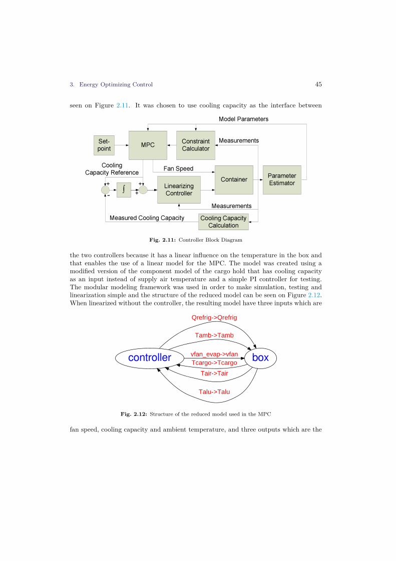
3. Energy Optimizing Control 45
seen on Figure 2.11. It was chosen to use cooling capacity as the interface between
ContainerLinearizingController
MPC
∫
ConstraintCalculator
+
+
-
Cooling CapacityCalculation
Measured Cooling Capacity
Cooling Capacity Reference
Model Parameters
Set-point
+
Fan SpeedParameter Estimator
Measurements
Measurements
Fig. 2.11: Controller Block Diagram
the two controllers because it has a linear influence on the temperature in the box andthat enables the use of a linear model for the MPC. The model was created using amodified version of the component model of the cargo hold that has cooling capacityas an input instead of supply air temperature and a simple PI controller for testing.The modular modeling framework was used in order to make simulation, testing andlinearization simple and the structure of the reduced model can be seen on Figure 2.12.When linearized without the controller, the resulting model have three inputs which are
controller box
Qrefrig->Qrefrig
Tamb->Tamb
vfan_evap->vfanTcargo->Tcargo
Tair->Tair
Talu->Talu
Fig. 2.12: Structure of the reduced model used in the MPC
fan speed, cooling capacity and ambient temperature, and three outputs which are the

46 Chapter 2. Summary of Work
temperatures of the air, the floor and the cargo. The linearizing controller between theMPC and the container shown on Figure 2.11 must follow the cooling capacity referenceas accurately as possible such that the system seen by the MPC resembles the reducedmodel. This is achieved through a nonlinear feed-forward that gives the compressorspeed and expansion valve opening degree that is required to provide the requestedcooling capacity and integrators to remove any errors. Because the cooling capacityreference is discrete, it is impossible to follow due to the time constants of the systemand therefore any accumulated cooling capacity error that is due to lag is removed bythe integrator shown in Figure 2.11.
The MPC minimize an objective function that must represent the cost of runningthe system at its current operating point and therefore the system COP was mappedfor different ambient temperatures, giving the result visible on Figure 2.13. The dotted
0 1 2 3 4 5 6 7 80
0.5
1
1.5
2
2.5
3
3.5
4
Tamb = 0°C
Tamb = 10°C
Tamb = 20°C
Tamb = 30°C
Tamb = 40°C
Tamb = 50°C
CO
P [−
]
Cooling Capacity [kW]
COP at setpoint −20°C
COPPWM
COPCOP
MAX
Fig. 2.13: The COP of the refrigeration system at varying ambient temperatures
line is the COP of the system when the compressor is running in PWM mode, where thecompressor is stopped and started with a duty cycle that matches the required cooling

3. Energy Optimizing Control 47
capacity. The reason for the sharp decline of COP in PWM mode is that the evaporatorfan continues running, while the compressor is off and therefore the contribution fromthe fan compared to the cooling capacity is increased as the duty cycle approaches zero.The ambient temperature has a big impact on both the level and the shape of the COPcurve and in order to effectively exploit this, the objective of the MPC must accuratelyreflect the cost over the length of the prediction horizon. This requires knowledge of thefuture ambient temperature which is not available, and therefore the predictor outlinedin section 3.3 is used.
The predicted ambient temperature is used to select the appropriate COP curveduring operation and the COP data is converted to a series of linear segments in theform y = ax + b that is used in an epigraph representation of the cost of running thecompressor in the constraints. The epigraph representation of the nonlinear natureof the COP ensures that a linear method can be used to solve the problem and thiscontributes to keeping the computational load of running the controller low. This isimportant in order to enable the controller to be run on embedded hardware, therebymaking the controller commercially interesting. Multi rate optimization step length [77]is introduced, to further reduce the computational load, while fine grained control ofthe present step is ensured.
Pc(k) + Vfan(k) · 195 + Ts(k) · 104 (2.8)
The objective function in Equation (2.8) consists of the epigraph variable that representsthe compressor power Pc, the cost of running the fan on low speed Vfan, and the slackvariable Ts that is introduced as a soft constraint in order to ensure that the problem canstill be solved if the temperatures drift outside the constraints due to model inaccuracies.
Vfan(k) · Qmin(k) ≤ Qcool(k) ≤ Vfan(k) · Qmax(k) (2.9)
Vfan−min ≤ Vfan(k) ≤ 1 (2.10)
Qcool(k) · a1(k) + b1(k) ≤ Pc(k) (2.11)
Qcool(k) · a2(k) + b2(k) ≤ Pc(k) (2.12)
Qcool(k) · a3(k) + b3(k) ≤ Pc(k) (2.13)
Qcool(k) · a4(k) + b4(k) ≤ Pc(k) (2.14)
0 ≤ Ts(k), (2.15)
Tcargo−min − Ts(k) ≤ Tcargo(k) ≤ Tcargo−max + Ts(k), (2.16)
Tair(k) < Tair−max + Ts(k) (2.17)
Equations (2.9) to (2.17) are the constraints where (2.9) and (2.10) are the actuatorlimits, and (2.11) to (2.14) are the constraints used in the piecewise affine epigraphrepresentation of the COP. The temperature constraints for the cargo and the air aregiven by Equation (2.16) and (2.17).
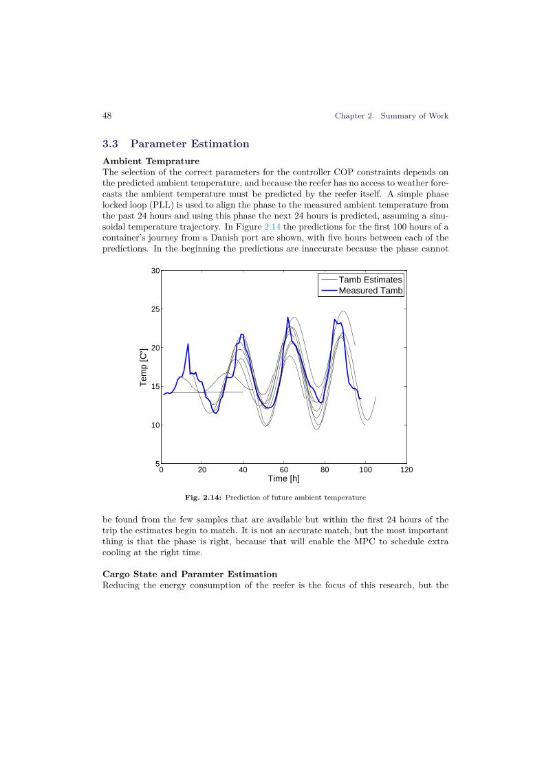
48 Chapter 2. Summary of Work
3.3 Parameter Estimation
Ambient TempratureThe selection of the correct parameters for the controller COP constraints depends onthe predicted ambient temperature, and because the reefer has no access to weather fore-casts the ambient temperature must be predicted by the reefer itself. A simple phaselocked loop (PLL) is used to align the phase to the measured ambient temperature fromthe past 24 hours and using this phase the next 24 hours is predicted, assuming a sinu-soidal temperature trajectory. In Figure 2.14 the predictions for the first 100 hours of acontainer’s journey from a Danish port are shown, with five hours between each of thepredictions. In the beginning the predictions are inaccurate because the phase cannot
0 20 40 60 80 100 1205
10
15
20
25
30
Time [h]
Tem
p [C
°]
Tamb EstimatesMeasured Tamb
Fig. 2.14: Prediction of future ambient temperature
be found from the few samples that are available but within the first 24 hours of thetrip the estimates begin to match. It is not an accurate match, but the most importantthing is that the phase is right, because that will enable the MPC to schedule extracooling at the right time.
Cargo State and Paramter EstimationReducing the energy consumption of the reefer is the focus of this research, but the

3. Energy Optimizing Control 49
most important objective of the controller is to ensure that the temperature of thecargo stays within its constraints, and while the parameters of the refrigeration systemare well known, there is no direct reliable temperature measurement of the cargo andthere are large uncertainties on its parameters. This makes it very difficult to ensurethat the constraints are not violated without reducing the allowed temperature range inorder to create safety zones which would impact the potential energy savings negatively.Therefore, an estimator for the latent cargo parameters was introduced. The estimatoris based on the model equations for the cargo hold and the cargo, and it estimates thefollowing latent variables:
Description UnitCargo heat capacity, Ccargo J/KCargo heat transfer coefficient, αcargo W/KCargo temperature, Tcargo
◦C
The estimator is based on the assumption that the system is Linear Time Invariant (LTI)and it derives that value of the parameters Ccargo and αcargo from two measurementsof the cargo at either end of a long period of sustained cooling at high capacity. The
−30
−25
−20
−15
−10
Tem
p [°
C]
T
sup
Tret
Tcargo
Tcargo−est
0 100 200 300 400 50010
20
30
40
50
60
Time [h]
[−]
α
cargo
Mcargo
Fig. 2.15: Startup of the cargo parameter estimator
50 Chapter 2. Summary of Work
reason for this is that in order to estimate the cargo dynamics they must be excited, andsince the thermal inertia of the cargo is very large, a significant amount of cooling mustbe applied before the dynamics can be estimated reliably through the air temperature.A first order filter with the air temperature as input and a time constant calculatedfrom Ccargo and αcargo, was used to estimate the cargo temperature. Therefore, theestimate of the cargo temperature will only be accurate if the parameters Ccargo andαcargo are correct. For a thorough description of the parameter estimator, please see[Paper D Section 2.2]. Figure 2.15 shows the result of the estimator running on datafrom a simulation of the model, with added measurement noise. The estimated heatcapacity of the cargo has been converted to mass in metric tons, using the specific heatcapacity for bacon which is 1050 J
kg·K[78]. The values of αcargo and Mcargo have been
scaled by 10 and 1000 respectively, in order to better show the details of the results.In this test, it is expected that αcargo levels out at 55 and that Mcargo level out at 20,and from the first update of the estimate the values are close to the real value. Theresulting estimated cargo temperature tracks the real value well and while there is someinaccuracy in the parameter estimates, it is deemed good enough for feedback control.
It is important that the estimator finds a set of parameters that makes the linearmodel behave the same way as the real system. If the model is inaccurate the estimatedparameters may also be inaccurate to compensate for the model inaccuracy, but aslong as the behavior of the model matches the real system this is not important. Theparameters from the estimator is applied to the linear model of the cargo hold beforeevery execution of the MPC and that ensures that the controller is able to perform wellon different types of cargo.
3.4 Results
The controller was tested in two different configurations, such that the energy savingsfrom reduced ventilation and exploitation of ambient temperature cycles could be iso-lated. Each configuration was run at three different ambient temperatures and the resultfrom the first 50 hours of the reference test and the two MPC configurations at 20◦Cambient temperature can be seen on Figure 2.16. The reference test is a PI controllerthat sets the cooling capacity reference to the linearizing controller and it is shown inthe two upper panels. This shows how the reefer would normally run with its currentcapacity controller; the cooling capacity is increased during the hotter periods, which isthe opposite of the desired behavior for reduced energy consumption.
The two panels in the middle show the results from the MPC where the fans arerunning continuously and it can be seen that the MPC uses the cargo’s thermal inertiato move cooling from cold to hot periods. The air and cargo temperature rise to itsupper constraint during the period where the ambient temperature is at its highest.The compressor is running in PWM most of the time because there is nothing to gainby running the compressor faster, at a lower efficiency, if it is not possible to turn off

3. Energy Optimizing Control 51
−22
−20
−18
TcargoTair
0
20
40
Cool ActCool ReqTamb
−22
−20
−18
TcargoTair
0
20
40
Cool ActCool ReqTamb
−22
−20
−18
TcargoTair
0 10 20 30 400
20
40
Time[h]
Cool ActCool ReqTamb
Fig. 2.16: Test results for the reference and the two test scenarios at 20◦C ambient temperature.
the fans for a longer period afterwards.The result from the test where the MPC is allowed to turn the fan off when the
compressor is not running, is shown in the two panels in the bottom of the figure. Thecompressor is no longer running PWM but instead at a higher capacity that allows thecompressor and fans to be turned off for longer periods, thus saving power. During theperiods of high ambient temperature the compressor is only turned on to keep the airtemperature within the constraints, while the cargo temperature is slowly increasingand this show that the controller behaves as intended.
The tests were all executed using the full simulation model of the container duringa 21 day simulation, in order to minimize the impact of any errors at the start of thesimulation. The model was simulated in a modular configuration and the full set oftests was completed in four days, which saved a lot of time compared to a real life test.The power savings found in the six tests are listed in the following table:

52 Chapter 2. Summary of Work
Ambient Temperature Fans Always ON Fans ON/OFF10 ± 5◦C 2.53% 21.9%20 ± 5◦C 3.07% 11.1%30 ± 5◦C 2.70% 3.96%
From the results it can be seen that the potential power savings are dependent onthe operating conditions and the reason for this is found in the way the refrigerationsystem is designed. It must be able to cool down a hot cargo within reasonable timeand therefore it runs at a small fraction of the available capacity when the cargo is atthe set-point, which is also where the system is most efficient. The COP curve for thecompressor alone is monotonically decreasing as the speed increases but when the powerfrom the fans is added, the COP curves shown in Figure 2.13 with a maximum in thelower capacity range emerge. This means that when the amount of cooling needed tokeep the set-point matches the most efficient capacity, the potential energy reductionfrom turning off the fans is zero and this is reflected by the results, that shows that theenergy savings decrease as the ambient temperature increases. When the most efficientmode of operation is running the system continuously, the cargo can still be used asa cooling storage and therefore there will always be something to gain from using thiscontrol strategy.
Studies of exploitation of large thermal inertias for reduction of energy consumptionor handling of peak demands in other applications have shown that it is often possibleto store significant amounts of cooling, leading to savings up to 30% or much improvedprevention of refrigeration system saturation. In [64] a learning based algorithm wasused to prevent saturation of system capacity in a supermarket refrigeration systembased on previous saturation events. This method has the advantage of being simpleand easily applied to an embedded system, but it would require some modificationsif it were to be used on a reefer due to the large variation in set points and cargotype that is transported. Different sets of learning data for each set point would haveto be stored and maintained by the controller and the method should be enhanced toconsider the economical aspect of the control problem. It has been shown in many worksthat the combination of MPC and large thermal inertias can yield considerable savings[63, 62, 79], and this is also reflected by the findings in this study.
In the present study the potential saving for the Star Cool reefer was investigatedand it was found that a saving between 2.5% and 3% is possible with a 10K variation inambient temperature. With a consumption of 8.9MW [80] for all the containers on a shipa 2.5% reduction yields 403.7GJ over a 21 day trip which is roughly 10000kg of heavyfuel oil. This results in a significant reduction in pollution and cost for transportationof refrigerated cargo, that will be even larger if the reduced ventilation rate is appliedas well. The six tests presented here show a big difference in potential savings andtherefore further experiments should be run to test the entire range of operation for thecontainer, but it is expected that the largest savings will be found where the differencebetween temperature set-point and ambient temperature is low.

3. Energy Optimizing Control 53
The investigation have uncovered the potential for energy savings in frozen reefercargo, by using the thermal inertia of the cargo as a buffer, and thereby objective IV isfulfilled.
3.5 Contributions
Proposal for a control strategy that is able to reduce the power consumption of a reeferthrough the use of the cargo as storage for cooling, and by being able to estimate impor-tant cargo parameters and adapt the controller accordingly. A series of optimizationson the MPC reduces the computational load and makes it commercially interesting.Adaptive model predictive control has not previously been used on a reefer, but thiswork shows that it is feasible, and that significant savings can be achieved.

54 Chapter 2. Summary of Work

Chapter 3
Conclusion
The work in this thesis concerns model based control for reefer containers used to trans-port perishable cargo worldwide. The aim of the project was to reduce the amountof energy consumed by the refrigeration system, without compromising the quality ofthe transported goods. The results of this work have been summarized in the previouschapters and the details are presented in the four papers that may be found in [Part II].In this chapter the conclusions of the research are presented and recommendations forfuture work and possible applications of the research are given.
1 Discussion
A model based controller was developed to handle the problems that exist on refrigeratedcontainers and tested using an accurate nonlinear simulation model of the system. Thecontributions in this project are divided in three categories: Modeling and Verification,Simulation and Controller Design and Validation. Objectives and requirements weredefined in Chapter 1 and subsequently verified in Chapter 2.
Modeling and VerificationObjective I described the need to create a non-linear dynamical model of the reefer withadequate accuracy for development of controllers and objective II described that thenon-linear dynamical model of the reefer was required to be formulated such that itcould be used as a simulation model for test and verification of controllers. An accuratemodel of the relevant parts of the container was created using a modular approach thatallows components to be changed easily when needed. The used methodology was basedon observations done on car air conditioning systems where it was found that the salientdynamics of the refrigeration system are defined by the thermal inertia of the metal in theheat exchangers, and this was shown to also be true for the larger refrigeration system
55

56 Chapter 3. Conclusion
in the Star Cool reefer. The model was verified against data from a real reefer withcargo. A collection of component models was selected from the literature and combinedinto a system model of the Star Cool reefer that showed good accuracy on the statesimportant for control. The modeling of the reefer and subsequent verification of themodel is presented in [Paper C]. In Section 1.4 it was concluded that the requirementswere fulfilled and objectives I and II had been reached.
SimulationObjective III stated that a simulation method, which met certain demands for speedand accuracy, had to be identified in order to enable a reduction in controller develop-ment time. Therefore, it was investigated how to most efficiently simulate the nonlinearmodel of the reefer, using a purpose made simulation framework for Matlab
R©, thatenabled simulation experiments in different configurations. An adaptation to a variablestep forward Euler solver was made, and when the resulting method was compared toMatlab
R©’s built-in solvers it was found to be significantly faster, while keeping compa-rable accuracy for simulations on the reefer model. It was investigated how monolithicand modular methods impacted the speed and accuracy of simulation on the model, andit was found that the modular method is faster when using Matlab
R© solvers. Whenthe adapted variable step forward Euler solver were used, there was no significant dif-ference between the modular and monolithic methods, but they were both faster thanwhen using Matlab
R©’s built-in solvers. The simulation framework and its associatedtools were used to verify the reefer model, and supported the development and testof the model based controller. The research has shown that it is possible to speed upsimulations of refrigeration systems using the modular method and shed light on theimplications of solver choice for modular simulation. Today the model is actively usedfor test and verification of controllers at Lodam, which have resulted in much shorterdevelopment time, due to the accuracy of the model and the high speed of the simula-tion. In Section 2.3 it was concluded that the requirements for simulation were fulfilledand that Objective III had been achieved.
Controller Design and ValidationObjective IV required an investigation of the potential energy savings by using thecargo as a storage for cooling and by reducing the ventilation rate. An adaptive modelpredictive controller was developed and tested using the simulation model and showedthat power savings of up to 21% can be achieved, by reducing the ventilation rateand using the cargo thermal inertia to store cooling. The largest savings were foundto originate from the reduced ventilation rate and found to be very dependent on theoperating point, but it is assessed that a typical container vessel will be able to saveat least 10000 kg of heavy fuel oil during a 21 day trip, if the proposed controller isapplied to the reefers on board. A parameter estimator for the unknown parametersand states of the cargo was introduced, and enabled the model predictive controller to
2. Perspective and Future Work 57
fully exploit the maximum allowed temperature variations of cargo and the air in thecontainer. The proposed controller consists of an inner loop controller that handlesthe fast refrigeration system dynamics and follows a cooling capacity reference that isgiven by the model predictive controller in the outer loop. This linearizes the nonlinearrefrigeration system from the perspective of the model predictive controller and greatlyreduces the problem that must be optimized, leading to a lower computational load. Arange of techniques were used to further reduce the computational load of the MPC, inorder to make it commercially interesting. The non-linear nature of the system COPwere embedded into the constraints using a piecewise affine epigraph representation,which ensured that the MPC problem could be solved using linear methods and multirate optimization step lengths were used to ensure fine grained control, while limitingthe size of the problem. In Section 3.4 it was verified that the proposed controllerfulfills the requirements and therefore objective IV, and the main objective of reducingthe energy consumption through model based control, have been reached.
2 Perspective and Future Work
In this section the perspectives of the scientific work in relation to other fields andrecommendations on future work are given.
2.1 Perspective
The nonlinear simulation model is very specific to the Star Cool reefer but due to themodular design it can easily be reconfigured to match other types of vapor compressionsystems, in for example heat pumps or cold storage facilities. The modeling metho-dology, where steady state equations for the refrigeration circuit are combined with adynamical model of the metal in the heat exchangers, has proven to be a good tradeoff between physical detail and accuracy and it is assessed that this methodology canbe used advantageously, for a large class of energy systems that have a phase change inthe working fluid.
The work done on simulation has highlighted some implications of the choice of simu-lation method and solver that may be useful in applications where large systems withvery different time constants are simulated. This type of system can be found withintransportation, aviation, process industry and energy systems.
The principle of the proposed controller structure, with an inner loop cooling capac-ity controller and an outer loop optimizing controller, works well for a reefer but thisstructure could also be used on other refrigeration systems with variable capacity. Theparameter and state estimator for the cargo requires that a model of the cargo holdis available to achieve acceptable accuracy. For other types of cold stores where the

58 Chapter 3. Conclusion
dynamics of the store itself are known and the details of the goods are unknown, anestimate may be acquired using the proposed estimator and thereby the possibility foroptimal exploitation of varying ambient temperature is achieved.
The tools that were developed to support the research will be beneficial to the taskof developing a unified, modern controller for the Star Cool reefer and the work hasshown that a flexible simulation environment can be built directly in Matlab
R©, result-ing in strong synergies with the available toolboxes.
2.2 Future Work
A model for the latent heat in moist air and buildup of ice on the evaporator would makethe simulation model of the reefer a more useful tool, because it would then be possibleto use it for optimization of defrost scheduling, and the injection controller could betested under more realistic conditions where the dynamics of the evaporator change asice builds up. It would also be beneficial to add the ability of tracking the location of theoil used to lubricate the compressor that circulates the refrigeration system. It wouldbe particularly useful to be able to predict oil accumulation in the evaporator and thedischarge of oil from the compressor, because this could be used to make a controllerthat ensure proper oil return to the compressor, at all times. The condenser model istoo simple and added physics could help improve the accuracy of the modeled dischargepressure.
The modeling and simulation tools would benefit from integration with an automaticparameter tuning tool such as Senstools, [81] that can tune the parameters of a model,based on recorded data from a real system. Advanced data exchange scheduling meth-ods are described in the literature and application of such a method, could provideguaranteed stability of the modular simulation and possibly also a higher simulationspeed. Alternatively, the current ZOH data exchange could be replaced by a simplerextrapolation method, such as a first or second order hold, which would increase speedand accuracy but not guarantee stability.
Development of a robust controller to replace the current feedback linearized innerloop capacity controller would improve system reliability under varying system charac-teristics. Fault tolerant control methods that are capable of self-reconfiguration shouldbe investigated such that the system may handle larger mechanical faults that cannotbe handled by the robust controller. Implementing a model predictive controller on anembedded system is deemed to be very demanding for the existing Star Cool controllerCPU, and therefore the problem should be reduced further or simpler methods shouldbe investigated. This could be in the form of a self learning controller that was adaptedto the present problem or a through a further reduction of the MPC problem. Explicit

2. Perspective and Future Work 59
solutions that reduce the quadratic problem of an MPC to a simple linear functionhas been described in the literature and could be used to enable implementation of thedeveloped control laws on the current reefers in the field.

60 References
References
[1] Lodam, “Lodam electronics homepage,” 2013. [Online]. Available: http://www.lodam.
com
[2] MCI, “Maersk container industry, starcool refrigerated container specifications,” 2013.[Online]. Available: http://www.maerskbox.com/
[3] D. S. C. Limited, “Reefer shipping market annual report,” Drewry House, 213 MarshWall, London, E14 9FJ,England, 2009. [Online]. Available: http://www.drewry.co.uk/get_file.php?id=1161
[4] Wageningen, “Agrotechnology & food sciences group, quest-leaflet,” 2015. [Online].Available: https://www.wageningenur.nl/upload_mm/d/6/b/2b3cd77e-4c34-4a62-95a9-1142267427de_Questleaflet2008.pdf
[5] S. Jonsson, “Performance simulations of twin-screw compressors with economizer,”International Journal of Refrigeration, vol. 14, no. 6, pp. 345 – 350, 1991. [Online].Available: http://www.sciencedirect.com/science/article/pii/014070079190031B.doi:10.1016/0140-7007(91)90031-B
[6] Carrier, “Carrier: Specifications for the primeline reefer,” 2006. [Online]. Available:http://www.container.carrier.com/StaticFiles/Carrier.com/Carrier%20Brand%20Sites%20Content/Carrier-Container/Files/Product_Solutions/Container_Equipment/PrimeLine.pdf
[7] ThermoKing, “Thermoking: Specifications for the magnumplus reefer,” 2011. [Online].Available: http://www.na.thermoking.com/content/dam/tki-na/pdf/Marketing%20Literature/60281_MagnumPlus_2011.pdf
[8] B. Rasmussen, Control-oriented Modeling of Transcritical Vapor Compression Systems.University of Illinois at Urbana-Champaign, 2002. [Online]. Available: http://books.google.dk/books?id=dQ0jywAACAAJ
[9] E. W. Grald and J. MacArthur, “A moving-boundary formulation for modelingtime-dependent two-phase flows,” International Journal of Heat and Fluid Flow, vol. 13,no. 3, pp. 266 – 272, 1992. [Online]. Available: http://www.sciencedirect.com/science/article/pii/0142727X9290040G. doi:http://dx.doi.org/10.1016/0142-727X(92)90040-G
[10] P. Mithraratne and N. Wijeysundera, “An experimental and numerical study of thedynamic behaviour of a counter-flow evaporator,” International Journal of Refrigeration,vol. 24, no. 6, pp. 554 – 565, 2001. [Online]. Available: http://www.sciencedirect.com/science/article/pii/S0140700700000530.doi:http://dx.doi.org/10.1016/S0140-7007(00)00053-0
[11] B. Rasmussen, A. Musser, and A. Alleyne, “Model-driven system identification oftranscritical vapor compression systems,” IEEE Transactions on Control SystemsTechnology, vol. 13, no. 3, pp. 444–451, 2005. doi:10.1109/TCST.2004.839572
[12] M. Willatzen, N. Pettit, and L. Ploug-Sørensen, “A general dynamic simulation modelfor evaporators and condensers in refrigeration. part i: moving-boundary formulation oftwo-phase flows with heat exchange,” International Journal of Refrigeration, vol. 21,
http://www.na.thermoking.com/content/dam/tki-na/pdf/Marketing%20Literature/60281_MagnumPlus_2011.pdf

References 61
no. 5, pp. 398 – 403, 1998. [Online]. Available: http://www.sciencedirect.com/science/article/pii/S0140700797000911. doi:10.1016/S0140-7007(97)00091-1
[13] N. Pettit, M. Willatzen, and L. Ploug-Sørensen, “A general dynamic simulation modelfor evaporators and condensers in refrigeration. part ii: simulation and control of anevaporator,” International Journal of Refrigeration, vol. 21, no. 5, pp. 404 – 414, 1998.[Online]. Available: http://www.sciencedirect.com/science/article/pii/S0140700797000923. doi:10.1016/S0140-7007(97)00092-3
[14] W.-J. Zhang and C.-L. Zhang, “A generalized moving-boundary model for transientsimulation of dry-expansion evaporators under larger disturbances,” InternationalJournal of Refrigeration, vol. 29, no. 7, pp. 1119 – 1127, 2006. [Online]. Available:http://www.sciencedirect.com/science/article/pii/S0140700706000570.doi:10.1016/j.ijrefrig.2006.03.002
[15] R. Shah, Dynamic Modeling and Control of Single and Multi Evaporator SubcriticalVapor Compression Systems. University of Illinois at Urbana-Champaign, 2003.[Online]. Available: http://books.google.dk/books?id=Tni2JgAACAAJ
[16] L.-X. Zhao, C.-L. Zhang, and B. Gu, “Neural-network-based polynomial correlation ofsingle- and variable-speed compressor performance,” HVAC&R Research, vol. 15, no. 2,pp. 255–268, 2009. [Online]. Available: http://www.tandfonline.com/doi/abs/10.1080/10789669.2009.10390836. doi:10.1080/10789669.2009.10390836
[17] H. Qiao, R. Rademacher, and V. Aute, “A review for numerical simulation of vaporcompression systems,” in Proceedings of 2010 International Refrigeration Conference,Purdue University, Indiana, USA, 2010. [Online]. Available: http://docs.lib.purdue.edu/cgi/viewcontent.cgi?article=2089&context=iracc
[18] H. Air-Conditioning and R. Institute, “Standard for positive displacement refrigerantcompressors and compressor units.” [Online]. Available: http://www.ari.org/App_Content/ahri/files/standards%20pdfs/ANSI%20standards%20pdfs/ANSI-ARI-540-2004%20latest.pdf
[19] C. Co, Flow of fluids through valves, fittings, and pipe, ser. Technical paper. Crane Co.,1988. [Online]. Available: http://books.google.dk/books?id=-fdRAAAAMAAJ
[20] D. Green and R. Perry, Perry’s Chemical Engineers’ Handbook, Eighth Edition, ser.McGraw Hill professional. McGraw-Hill Education, 2007. [Online]. Available: http://books.google.dk/books?id=tH7IVcA-MX0C
[21] R. Miller, Flow measurement engineering handbook, ser. Chemical engineering books.McGraw-Hill, 1996. [Online]. Available: https://books.google.dk/books?id=0e9RAAAAMAAJ
[22] H. Li and J. E. Braun, “A method for modeling adjustable throat-area expansion valvesusing manufacturers rating data,” HVAC&R Research, vol. 14, no. 4, pp. 581–595, 2008.[Online]. Available: http://www.tandfonline.com/doi/abs/10.1080/10789669.2008.
10391027. doi:10.1080/10789669.2008.10391027
[23] T. Zaleski and K. Klepacka, “Approximate method of solving equations for plate heatexchangers,” International Journal of Heat and Mass Transfer, vol. 35, no. 5, pp. 1125 –

62 References
1130, 1992. [Online]. Available: http://www.sciencedirect.com/science/article/pii/001793109290173P. doi:10.1016/0017-9310(92)90173-P
[24] S. K. Al-Dawery, A. M. Alrahawi, and K. M. Al-Zobai, “Dynamic modeling and controlof plate heat exchanger,” International Journal of Heat and Mass Transfer, vol. 55, no.23-24, pp. 6873 – 6880, 2012. [Online]. Available: http://www.sciencedirect.com/science/article/pii/S001793101200525X. doi:10.1016/j.ijheatmasstransfer.2012.06.094
[25] J. Kay and R. Nedderman, Fluid Mechanics and Transfer Processes. CambridgeUniversity Press, 1985. [Online]. Available: https://books.google.dk/books?id=43U7AAAAIAAJ
[26] K. Prölss, G. Schmitz, D. Limperich, and M. Braun, “Influence of refrigerant chargevariation on the performance of an automotive refrigeration system,” in InternationalRefrigeration and Air Conditioning Conference, Paper 843, 2006. [Online]. Available:http://docs.lib.purdue.edu/iracc/843
[27] Guo-liang Ding, “Recent developments in simulation techniques for vapour-compressionrefrigeration systems,” International Journal of Refrigeration, vol. 30, no. 7, pp.1119–1133, 2007. doi:10.1016/j.ijrefrig.2007.02.001
[28] “Trnsys.” [Online]. Available: http://sel.me.wisc.edu/trnsys/
[29] M. Skovrup, “Windali - an open-structured component modeling and simulationprogram based on standard programming languages,” in Proceedings of SIMSConference. Lyngby, 2000, pp. 157–172.
[30] “Dymola.” [Online]. Available: http://www.dynasim.se/index.htm
[31] P. Fritzson and P. Bunus, “Modelica – a general object-oriented language for continuousand discrete-event system modeling,” in IN PROCEEDINGS OF THE 35TH ANNUALSIMULATION SYMPOSIUM, 2002, pp. 14–18.
[32] L. Liu, F. Felgner, and G. Frey, “Comparison of 4 numerical solvers for stiff and hybridsystems simulation,” in Emerging Technologies and Factory Automation (ETFA), 2010IEEE Conference on, Sept 2010, pp. 1–8. doi:10.1109/ETFA.2010.5641330
[33] L. F. Shampine and M. W. Reichelt, “The matlab ode suite,” Journal on ScientificComputing, vol. 18, pp. 1–22, 1997. doi:10.1137/S1064827594276424
[34] C. Rosen, D. Vrecko, K. Gernaey, and U. Jeppsson, “Implementing adm1 for benchmarksimulations in matlab/simulink,” Journal of Water science and technology, vol. 54, no. 4,pp. 11–19, 2006. doi:10.2166/wst.2006.521
[35] R. M. Howe, “Accuracy and stability tradeoffs in multirate simulation,” in Proceedings ofSPIE, vol. 4367, 2001, pp. 113–126. doi:10.1117/12.440011
[36] J. G. Pearce, R. E. Crosbie, J. J. Zenor, R. Bednar, D. Word, and N. G. Hingorani,“Developments and applications of multi-rate simulation.” in UKSim, D. Al-Dabass, Ed.IEEE, 2009, pp. 129–133. [Online]. Available: http://dblp.uni-trier.de/db/conf/uksim/uksim2009.html#PearceCZBWH09. doi:10.1109/UKSIM.2009.23
[37] R. Kübler and W. Schiehlen, “Modular simulation in multibody systems,” MultibodySystem Dynamics, vol. 4, pp. 107–127, 2000. doi:10.1023/A:1009810318420

References 63
[38] J. Läckel, F. Junker, and S. Toepper, “Block-oriented modelling of rigid multibodysystems with regard to subsystem techniques,” in Advanced Multibody System Dynamics,ser. Solid Mechanics and Its Applications, W. Schiehlen, Ed. Springer Netherlands,1993, vol. 20, pp. 49–66. [Online]. Available: http://dx.doi.org/10.1007/978-94-017-0625-4_3. doi:10.1007/978-94-017-0625-4_3
[39] R. Kübler and W. Schiehlen, “Two methods of simulator coupling,” Mathematical andComputer Modelling of Dynamical Systems, vol. 6, no. 2, pp. 93–113, 2000. [Online].Available: http://www.tandfonline.com/doi/abs/10.1076/1387-3954%28200006%296%3A2%3B1-M%3BFT093. doi:10.1076/1387-3954(200006)6:2;1-M;FT093
[40] J. Butcher, “General linear methods for ordinary differential equations,” Mathematicsand Computers in Simulation, vol. 79, no. 6, pp. 1834 – 1845, 2009, applied andComputational MathematicsSelected Papers of the Sixth PanAmerican WorkshopJuly23-28, 2006, Huatulco-Oaxaca, Mexico. [Online]. Available: http://www.sciencedirect.com/science/article/pii/S0378475407001462.doi:http://dx.doi.org/10.1016/j.matcom.2007.02.006
[41] J. C. Butcher, “General linear methods,” Acta Numerica, vol. 15, pp. 157–256, 5 2006.[Online]. Available: http://journals.cambridge.org/article_S0962492906220014.doi:10.1017/S0962492906220014
[42] J. Butcher, “General linear methods,” Computers & Mathematics with Applications,vol. 31, no. 4-5, pp. 105 – 112, 1996, selected Topics in Numerical Methods. [Online].Available: http://www.sciencedirect.com/science/article/pii/0898122195002227.doi:http://dx.doi.org/10.1016/0898-1221(95)00222-7
[43] U. Ascher and L. Petzold, Computer Methods for Ordinary Differential Equations andDifferential-Algebraic Equations. Society for Industrial and Applied Mathematics, 1998.[Online]. Available: http://books.google.dk/books?id=AqQ6QMthXkMC
[44] J. C. Butcher, Numerical methods for ordinary differential equations. J. Wiley, 2003.[Online]. Available: http://www.worldcat.org/isbn/9780471967583
[45] K. Atkinson, An introduction to numerical analysis. Wiley, 1978. [Online]. Available:http://books.google.dk/books?id=ByPpQ1nt3esC
[46] K. J. AAström and T. Hägglund, PID Controllers: Theory, Design, and Tuning, 2nd ed.Instrument Society of America, Research Triangle Park, NC, 1995.
[47] G. F. Franklin, D. J. Powell, and A. Emami-Naeini, Feedback Control of DynamicSystems, 4th ed. Upper Saddle River, NJ, USA: Prentice Hall PTR, 2001.
[48] H. K. Khalil and J. Grizzle, Nonlinear systems. Prentice hall Upper Saddle River, 2002,vol. 3.
[49] W. Leithead, “Survey of gain-scheduling analysis design,” International Journal ofControl, vol. 73, pp. 1001–1025, 1999.
[50] J. Shamma and M. Athans, “Gain scheduling: potential hazards and possible remedies,”Control Systems, IEEE, vol. 12, no. 3, pp. 101–107, June 1992. doi:10.1109/37.165527
[51] F. Wu, “Control of linear parameter varying systems,” Ph.D. dissertation, University ofCalifornia, 1995.

64 References
[52] G. J. Balas, “Linear, parameter-varying control and its application to a turbofan engine,”International Journal of Robust and Nonlinear Control, vol. 12, no. 9, pp. 763–796, 2002.[Online]. Available: http://dx.doi.org/10.1002/rnc.704. doi:10.1002/rnc.704
[53] I. Postlethwaite, Multivariable Feedback Control: Analysis and Design. New York, NY,USA: John Wiley & Sons, Inc., 1996.
[54] G. J. C. Verdijck, “Model-based product quality control applied to climate controlledprocessing of agro-material,” 2003. [Online]. Available: http://alexandria.tue.nl/extra2/200310443.pdf
[55] G. J. C. Verdijck, M. Weiss, and H. A. Preisig, “Model-based product quality control fora potato storage facility,” in American Control Conference, 1999. Proceedings of the1999, vol. 4, 1999, pp. 2558–2562 vol.4. doi:10.1109/ACC.1999.786522
[56] G. J. C. Verdijck and G. van Straten, “A modelling and control structure for productquality control in climate-controlled processing of agro-material,” Control EngineeringPractice, vol. 10, no. 5, pp. 533 – 548, 2002. [Online]. Available: http://www.
sciencedirect.com/science/article/pii/S0967066102000035.doi:10.1016/S0967-0661(02)00003-5
[57] G. J. C. Verdijck, G. van Straten, and H. Preisig, “Optimisation of product quality andminimisation of its variation in climate controlled operations,” Computers andElectronics in Agriculture, vol. 48, no. 2, pp. 103–122, 2005.doi:10.1016/j.compag.2005.02.009
[58] R. G. M. van der Sman and G. J. C. Verdijck, “Model predictions and control ofconditions in a ca-reefer container,” in ISHS Acta Horticulturae 600: VIII InternationalControlled Atmosphere Research Conference, Agrotechnological Research Institute ATO,P.O. box 17, 6700 AA Wageningen, the Netherlands, 2003, pp. 163–171. [Online].Available: http://www.actahort.org/members/showpdf?booknrarnr=600_20
[59] J. Maciejowski, Predictive Control: With Constraints, ser. Pearson Education. PrenticeHall, 2002. [Online]. Available: http://books.google.dk/books?id=HV_Y58c7KiwC
[60] A. Bemporad, M. Morari, V. Dua, and E. Pistikopoulos, “The explicit solution of modelpredictive control via multiparametric quadratic programming,” in American ControlConference, 2000. Proceedings of the 2000, vol. 2, 2000, pp. 872–876 vol.2.doi:10.1109/ACC.2000.876624
[61] A. Bemporad, M. Morari, V. Dua, and E. N. Pistikopoulos, “The explicit linearquadratic regulator for constrained systems,” Automatica, vol. 38, no. 1, pp. 3 – 20, 2002.[Online]. Available: http://www.sciencedirect.com/science/article/pii/S0005109801001741. doi:http://dx.doi.org/10.1016/S0005-1098(01)00174-1
[62] L. S. Larsen, C. Thybo, and H. Rasmussen, “Intelligent control - optimizing theoperation of refrigeration systems under daily variations in ambient temperature,” inDanske Køledage, March 15th-16th, 2007. Proceedings of Danske Køledage 2007., 2007.
[63] J. Cai, J. Stoustrup, and J. Jorgensen, “Preventing refrigerated foodstuffs insupermarkets from being discarded on hot days by mpc,” in Proceedings of the 17th IFACWorld Congress, Seoul, Korea, 2008. [Online]. Available: http://www.control.aau.dk/~jakob/selPubl/papers2008/ifacwc_2008_3.pdf. doi:10.3182/20080706-5-KR-1001.01880
References 65
[64] K. Vinther, H. Rasmussen, R. Izadi-Zamanabadi, J. Stoustrup, and A. Alleyne,“Learning-based precool algorithms for exploiting foodstuff as thermal energy reserve,”Control Systems Technology, IEEE Transactions on, vol. PP, no. 99, pp. 1–1, 2014.doi:10.1109/TCST.2014.2328954
[65] A. Jakobsen, B. Rasmussen, and M. Skovrup, “Development of energy optimal capacitycontrol in refrigeration systems,” in Proceedings of 2000 International RefrigerationConference. Purdue University, Indiana, USA: http://docs.lib.purdue.edu/cgi/viewcontent.cgi?article=1498&context=iracc, 2000, pp. 329–336.
[66] R. Zhou, T. Zhang, J. Catano, J. T. Wen, G. J. Michna, Y. Peles, and M. K. Jensen,“The steady-state modeling and optimization of a refrigeration system for high heat fluxremoval,” Applied Thermal Engineering, vol. 30, no. 16, pp. 2347 – 2356, 2010. [Online].Available: http://www.sciencedirect.com/science/article/pii/S135943111000219X.doi:10.1016/j.applthermaleng.2010.05.023
[67] R. Koury, L. Machado, and K. Ismail, “Numerical simulation of a variable speedrefrigeration system,” International Journal of Refrigeration, vol. 24, no. 2, pp. 192 –200, 2001. [Online]. Available: http://www.sciencedirect.com/science/article/pii/S0140700700000141. doi:10.1016/S0140-7007(00)00014-1
[68] B. P. Rasmussen and A. G. Alleyne, “Control-oriented modeling of transcritical vaporcompression systems,” Journal of dynamic systems, measurement, and control, vol. 126,no. 1, pp. 54–64, 2004.
[69] B. Rasmussen and A. Alleyne, “Dynamic modeling and advanced control of airconditioning and refrigeration systems,” Air Conditioning and Refrigeration Center.College of Engineering. University of Illinois at Urbana-Champaign., 2006. [Online].Available: http://hdl.handle.net/2142/12355
[70] “MatlabR©- ordinary differential equation solvers.” [Online]. Available: http://www.
mathworks.se/help/matlab/ordinary-differential-equations.html
[71] C. B. Brosilow, Y.-C. Liu, J. Cook, and J. Klatt, “Modular Integration Methods forSimulation of Large-Scale Dynamic Systems,” Modeling, Identification and Control,vol. 6, no. 3, pp. 153–179, 1985. doi:10.4173/mic.1985.3.4
[72] S. Skogestad and I. Postlethwaite, Multivariable Feedback Control: Analysis and Design,2nd ed. Wiley, 2005. [Online]. Available: http://eu.wiley.com/WileyCDA/WileyTitle/productCd-047001167X.html
[73] F. Wu, “Control of linear parameter varying systems,” Ph.D. dissertation, University ofCalifornia, 1995. [Online]. Available: http://www.mae.ncsu.edu/wu/paper/PhDthesis.ps
[74] D. Petersson and J. Löfberg, “LPV H2-controller synthesis using nonlinearprogramming,” in Proceedings of the 18th IFAC World Congress :, 2011, pp. 6692–6696.doi:10.3182/20110828-6-IT-1002.02028
[75] “MatlabR©
SimulinkR© linearization algorithm.” [Online]. Available: http://www.
mathworks.se/help/slcontrol/ug/exact-linearization-algorithm.html
[76] E. Kreyszig, Advanced Engineering Mathematics, 9th ed. Wiley, Nov. 2005. [Online].Available: http://www.amazon.com/exec/obidos/redirect?tag=citeulike07-20&path=ASIN/0471488852

66 References
[77] U. Halldorsson, M. Fikar, and H. Unbehauen, “Nonlinear predictive control withmultirate optimisation step lengths,” IEE Proceedings - Control Theory andApplications, vol. 152, no. 3, pp. 273–285, 2005. doi:10.1049/ip-cta:20041310
[78] “Specific heats of common food and foodstuff,” 2015. [Online]. Available: http://www.
engineeringtoolbox.com/specific-heat-capacity-food-d_295.html
[79] R. Halvgaard, N. K. Poulsen, H. Madsen, and J. B. Jorgensen, “Economic modelpredictive control for building climate control in a smart grid,” in Innovative Smart GridTechnologies (ISGT), 2012 IEEE PES, IEEE. http://orbit.dtu.dk/fedora/objects/orbit:74519/datastreams/file_6543920/content, 2012, pp. 1–6.
[80] Container-Handbook, “8.1.2 actual power consumption,” 2009. [Online]. Available:http://www.containerhandbuch.de/chb_e/wild/index.html?/chb_e/wild/wild_08_01_02.html
[81] M. Knudsen, Senstools: A Matlab Toolkit for Parameter Estimation in Linear andNonlinear Systems Using a Sensitivity Approach. Department of Control Engineering,Aalborg University, 1996. [Online]. Available: http://books.google.dk/books?id=ygHPQwAACAAJ

Part II
Papers
67


Paper A
Modular Modeling and Simulation Approach - Applied to
Refrigeration Systems
Kresten K. Sørensena,b and Jakob Stoustrupa
aSection for Automation and Control, Department of Electronic Systems
Aalborg University, Fredrik Bajers Vej 7C, 9220 Aalborg, DenmarkbLodam electronics a/s, Kærvej 77, 6400 Sønderborg, Denmark
E-mail: [email protected] [email protected]
The paper has been published in the proceedings of the2008 IEEE Multi-conference on Systems and Control , pp. 983-988.

2008 IEEEThe layout has been revised.
1. Introduction 71
Abstract
This paper presents an approach to modeling and simulation of the thermal dynamics of arefrigeration system, specifically a reefer container. A modular approach is used and theobjective is to increase the speed and flexibility of the developed simulation environment.The refrigeration system is divided into components where the inputs and outputs aredescribed by a set of XML files that can be combined into a composite system modelthat may be loaded into Matlab
R©. A set of tools that allows the user to easily loadthe model and run a simulation are provided. The results show a simulation speed-upof more than a factor of three by partitioning the model into smaller parts, and therebyisolating fast and slow dynamics. As a cost there is a reduction in accuracy which inthe example considered is less than one percent.
1 Introduction
Numerical simulation is extensively used for experiments within the field of controlengineering, and with the increasing power of computers it has become possible tosimulate very large dynamical systems on a normal desktop PC at reasonable speed.But larger system models results in larger and more complex equation sets that aredifficult to handle and therefore a range of simulation tools capable of handling largesystem models is available. When choosing a simulation tool it is worth considering theease of modeling, simulation speed and accuracy because these parameters vary fromtool to tool.
A common tool utilized within control engineering is SimulinkR© [1], which allows
the user to create and simulate large models from built-in or user developed componentlibraries through a Graphical User Interface (GUI). The simulation model composed ofcomponent models may be solved by a range of block oriented input/output solvers thatautomatically adjusts the size of the numerical integration step. Simulink
R© variable-step solvers change the step size during simulation [2], reducing the step size to increaseaccuracy when the states of a simulation model are changing rapidly and increasingthe step size to avoid taking unnecessary steps when the models states are changingslowly. Computing the step size adds to the computational overhead at each step butcan reduce the total number of steps, and hence simulation time, required to maintaina specified level of accuracy for models with rapidly changing or piecewise continuousstates. The selected integrations step is however inherited by blocks further down thesignal path and if the components further down the path have slow dynamics comparedto the preceding blocks they will be simulated with unnecessarily small integration stepsizes, leading to a computational overhead. Such a system is referred to as stiff andwhile Matlab
R© and SimulinkR© have specific solvers for these types of problems they
do not address the problem with computational overhead in stiff systems.

72 Paper A.
Another approach is used by Dymola [3] that implements the Modelica [4] lan-guage which is an equation-based object-oriented modelling language. In Modelica
symbolic equations that define the dynamical behavior of a component may be enteredin a non-causal way, leaving the task of ordering and reducing the final set of equationsto the simulation engine before a simulation can be run. Stiff problems may be solvedusing implicit methods that allow larger step-sizes at the cost of solving a set of non-linear equations at each time step. Dymola uses mixed-mode integration [5] that takesa middle course where the system is split up into fast and slow states. Only the faststates are discretized implicitly leaving a smaller set of nonlinear equations to solve ateach time step and thus a faster simulation. To speed up the simulation even furtherinline integration [6] is supported. The discretization formulas are inserted (in-lined)into the problem and Dymola’s symbolic engine is applied to the resulting equations[5]. The automatic model reduction and partitioning approach used by Dymola doesnot, however, take advantage of a-priori system knowledge that already exists.
In this paper an attempt was made to build a small and fast simulation environmentthat provides easy modular modelling and rapid prototyping of refrigeration systemsfrom a library of component models. A modelling and simulation environment forMatlab
R© has been developed to enable simulation experiments on nonlinear modelsconsisting of a mix of models based on Ordinary Differential Equations (ODE), Dif-ferential Algebraic Equations (DAE) and purely algebraic equations. The objective ofthe tool is to provide rapid and flexible refrigeration system model development from apredefined set of refrigeration component models. A refrigeration container model hasbeen chosen as an example for this study.
Refrigeration containers are used to move many different types of cargo betweenall areas in the world and this puts some unusual requirements on the refrigerationsystem with respect to the temperature range on both the cold and the hot side. Thegoods transported may require a stable temperature between -30C◦ and +20C◦ andthe temperature of the air around the container can be between -30C◦ and +50C◦.Because of the nonlinear nature of the refrigeration system and the large temperaturerange it is infeasible to use a linear model for simulation experiments and therefore anonlinear model must be used. The requirements for such a model is that it shouldmatch the real system close enough to be used for closed loop control experiments andsimulations should run at least one order of magnitude faster than experiments on thereal system. Another important requirement is that it must be possible to change themodel configuration without having to rewrite or reorganize the entire set of equationsfor the model by hand. Therefore a modular approach is selected where the model ofthe refrigeration system is composed of a set of interchangeable component models thatare based on first principles and assumptions where appropriate.
A model of a refrigeration container is developed and used as a test case for thesimulation environment. The system has both fast and slow states but the fast statesare isolated in a single component leading to a potential speed-up of the simulation with

2. Modelling 73
a modular approach. Therefore it was attempted to decouple component models withslower dynamics from models with fast dynamics by simulating each of the componentmodels separately and only exchange input/output values between the component mo-dels at fixed discrete times. The number of steps and average step time for the solversfor each of the components is used to calculate the difference in simulation time of theexample system, as either a modular model or a monolithic model.
2 Modelling
The model of the refrigeration system is divided into components that each represent aphysical component of the system, i.e. a condenser or an evaporator. Each componentmodel is described by two files; an m file that holds the input/output equations of themodel and an XML file that describes the properties of the inputs and outputs of them file. The simulation model is the overall model for the refrigeration plant and itsproperties are described by an XML file that holds a list of included component modelsand the connections between them. Therefore the structure of the simulation modelis defined by the simulation model definition file, and from this the model loader cancreate a simulation object that is used by the simulator.
2.1 Component Model Syntax
Modelling of component models is basically the same as for normal ODE model functionsthat may be solved by Matlab
R©’s built-in ode solvers, but additional info is needed bythe model loader in order to do type-checking when connecting the inputs and outputsof the component models. Each component model is described by an m file containingthe input/output equations, an XML file describing the input/output properties of themodel, its execution mode, and the name of the corresponding m file. The syntax forwriting the component model XML file is shown in the box below:

74 Paper A.
Listing A.1: Component Model Syntax
<?xml version="1.0" encoding="UTF-8"?>
<component name=["Component Name]">
<inputs>
<input name=["Input1 Name"] type=["Input1 Type"]
description=["Input1 Description"]/>
.
.
<input name=["InputN Name"] type=["InputN Type"]
description=["InputN Description"]/>
</inputs>
<states>
<state name=["State1 Name"] type=["State1 Type"]
default=["State1 Start Value"]
description=["State1 Description"]/>
.
.
<state name=["StateN Name"] type=["StateN Type"]
default=["StateN Start Value"]
description=["StateN Description"]/>
</states>
<connectors>
<connector type=["type"] conid=["Conn. Name"]>
<{input, state} name=["Name"]
type="Physical Entity"/>
<{input, state} name=["Name"]
type="Physical Entity"/>
</connector>
.
.
</connectors>
<control_inputs>
<input name=["Input Name"] type=["Input Type"]
description=["Input Description"]/>
.
.
</control_inputs>
<simulation method={"ode15s", "call"}
call=[".m File Function Name"]/>
<filename>[.m File Name]</filename>
</component>
The <inputs> section contains a list of the inputs to the component model, and it isimportant that the inputs are listed in the same order as they occur in the input vectorof the model function. Each input has a name, a type used for type-checking when
2. Modelling 75
inputs are connected, and a description. There must be the same number of inputs inthe input list as the length of the input vector of the corresponding model function.The <states> section is similar to the input section except that it describes the states oroutputs of the function and that a default value must be declared. The default value isused as initial value in simulations when the simulation tool is not given an initial statevector to start from. Signals may be grouped together in connectors that allows theuser to connect a set of signals from one component model to a similar set on anothercomponent model in one operation.
Because this environment is used for refrigeration systems it has a built-in connec-tor class for refrigeration pipe interfaces but obviously, for other applications, otherconnections will be relevant - see Simulation Model Syntax in Subsection II.B. On therefrigeration pipe interface three variables exist; a mass flow m, a pressure p, and an en-thalpy h. The model loader will return an error if each refrigeration pipe interface doesnot contain exactly one of each of the mentioned aforementioned types. The individualvariables may be either an input or a state but the model loader will check that each ofthe inputs can be connected to a state of the correct type when two refrigeration pipeinterfaces are connected. This saves the user the work of having to connect the variablesmanually, but when building the component models attention must be given to wherethe different states that are shared between models are located.
2.2 Simulation Model Syntax
The syntax for the simulation model XML file are listed below:

76 Paper A.
Listing A.2: Simulation Model Syntax
<?xml version="1.0" encoding="UTF-8"?>
<simulation_model name=["Simulation Model Name"]>
<component_path>[Component Library Path]
</component_path>
<components>
<component name=["Component Model Name"]
file=["Component Model XML File Name"]/>
.
.
<component name=["Component Model Name"]
file=["Component Model XML File Name"]/>
</components>
<connections>
<connector name=["Connector Name"]>
<component name=["Component Name"]
conid=["Connection Name"]/>
<component name=["Component Name"]
conid=["Connection Name"]/>
</connector>
<connection name=["Connection Name"]>
<component name=["Component Name"]
type="Input" input=["Input Name"]/>
<component name=["Component Name"]
type="Output" output=["Output Name"]/>
</connection>
</connections>
</simulation_model>
The simulation model is composed of a set of component models and their connec-tions described by the simulation model XML file, containing a list of the included compo-nent models and a description of how the components are connected. The <components>
section lists the component models used in the simulation model and it is allowed to usea component model more than once if they are given unique names. In the <connections>
section all the connections in the simulation model are listed. A connector connectionis established as in the <connector> sections by giving the name of the two componentmodels and the connector on each of the components. Inputs and outputs that are notassociated with connector interfaces, such as control inputs to actuators, are connectedin a <connection> section by listing the two components one by one. In each of the<component> sections it must be stated whether the signal is an input or an output, andwhat the name of the signal is. The model loader provides type checking on connectionsbetween components and gives a precise description, with the names of the implicated

3. Simulation 77
components and signals, in case of an eventual error in the set of connections betweencomponents.
The model may be loaded into MatlabR© with a model loader function that loads
each of the components and creates a struct containing all the information necessary forsimulation. During simulation the states of the component models are kept in a singlevector, denoted X, and therefore two matrices that maps between X and componentmodel I/O are generated for each component model. The matrix Zn maps from X tothe component model x-vector xn such that
X = Zn · xn (A.1)
xn = ZTn · X (A.2)
where the index n denotes the component model number. Component model inputs un
are mapped from X by the matrix CMn such that
un = CMn · X (A.3)
Because CMn maps from state variables that reflect a physical value to inputs thattake a physical value, it is a one-zero matrix and must have exactly one "1" in each row.When the model loader has created the mapping matrices they are used to check theconnection integrity of the system model such that all inputs are connected to exactlyone state.
3 Simulation
Simulation of the system model is done in discrete time steps defined in the time vectorgiven in the simulation function call. In each of the time steps the component modelsare simulated separately, according to the method defined in the component model XML
file and the results are then combined into the X vector containing the states for all ofthe component models. Component models that are purely algebraic are evaluated inone operation like a normal Matlab
R© function, and dynamical models are solved byone of Matlab
R©’s built-in ode functions. Fig. (A.1) shows a possible structure for asimulation model consisting of four component models.
The discretization of the signals between the component models is equivalent toinserting a zero order hold between all models as shown on Fig. (A.1).
The input to the individual component models are calculated by applying (A.2) and(A.3) and given as arguments to the appropriate simulation function such that
xn(k) = fn ([t(k − 1) t(k)], Zn · xn, CMn · X) (A.4)
where fn is the simulation function for the referenced component model and [t(k −1) t(k)] is the time interval in which to simulate. The results from the each of the

78 Paper A.
Fig. A.1: Example of a Simulation Model Structure
component simulations are then combined into the system state-vector X by
X(k) =
N∑
n=1
Zn · xn(k) (A.5)
where N is the total number of components in the model. The simulation environmentmay then proceed and simulate the next time step with the same procedure as above.
4 Reefer Model
The refrigeration system used as an example here utilize an economizer to increase theefficiency of the system at high pressure differences between the cold and hot side. Thecompressor efficiency is lower at high pressure differences which is exist when there isa large difference between the evaporation and condensation temperatures.The econo-mizer arrangement increases the refrigeration capacity and improves the coefficient ofperformance (COP) [7]. A schematic of the system can be seen in Fig. A.2. The ele-ments of the model are described in the sequel. The explicit 44 equations of the modelare not derived here due to space limitations, but they are available in [8].
The system consists of a two-stage piston compressor, a condenser, an evaporator,and an economizer [7] which is a counterflow plate heat exchanger. The compressor isequipped with a frequency converter which enables it to run at variable speed. Theexpansion valves are electromagnetically pulsed on/off valves and the fans may run at

4. Reefer Model 79
Fig. A.2: Refrigeration System for a Reefer Container
half speed, full speed, or be turned off entirely. There are three major pressure levels inthis setup; p1 is the evaporator pressure, p2 is the intermediate pressure between the twocompressor stages, and p3 is the condenser pressure. Since p2 is also the evaporationpressure on the cold side of the economizer it is coupled closely to the evaporationtemperature of the economizer, and hence influential on the inlet temperature of therefrigerant to the evaporator.
According to [9] the dominant dynamics of a refrigeration system are the thermaltime constants of the metal surfaces in the heat exchangers and refrigerant mass timeconstants, with respect to control applications. Also according to [9] some of the com-ponents have dynamics that are so fast compared to the dominant dynamics that theymay be replaced with algebraic equations, thus reducing the model order while preserv-ing the physical behavior of the model on the dominant dynamics. The componentsthat may be modeled algebraically are the expansion valves and the compressors whilethe rest of the components are modeled using first principles or assumptions. Two pipejunction models are needed in order to model the joining and splitting of refrigerantflows that occur between the compressor stages and after the receiver, respectively.
4.1 Pipe Joining Junction
The pipe junction model has three states; Pressure p, internal mass M , and outputenthalpy hout. It also has five inputs; the mass flows on all three interfaces min1, min2,mout, and the input enthalpy for both refrigerant inputs hin1 and hin2. The pressureof this component model has fast dynamics because it is a small volume containingvapor with a high mass flow and no boiling liquid to dampen pressure oscillations and
80 Paper A.
therefore the exact dynamics are neglected and the absolute pressure simply calculatedinstead.
4.2 Compressor
The compressor has two almost identical stages where the only difference is that thedisplacement volume of the first stage is twice as large as that of the second stage. Thecompressor stages are modelled by two algebraic functions giving the mass flow andoutput enthalpy as a function of input pressure, output pressure, input enthalpy, thespeed of the compressor, and the temperature of the compressor. The compression isassumed adiabatic and the physical behavior of the model includes harmful volume,and valve pressure loss. The mass of the refrigerant in the compressor is neglected andtherefore the mass flows on the input and output are equal.
4.3 Expansion Valve
The expansion valve model is purely algebraic and modelled as a continuous valve givingthe average mass flow of the electromagnetically pulsed on/off valves used on the reefer.A lookup table is used to find the mass flow at full opening as a function of the pressureson both sides and this is multiplied with the ON time, which is the fraction of time itis turned on. The expansion is assumed adiabatic end therefore there is no change tothe enthalpy of the refrigerant.
4.4 Economizer
The hot side of the economizer is filled with liquid refrigerant running from the receiverto the evaporator expansion valve and is therefore modelled as a single region withuniform heat transfer from liquid to metal. The liquid volume is assumed to haveuniform pressure and enthalpy and a constant pressure drop from input to output. Thecold side, where refrigerant evaporates, is modelled as a single volume where the amountof energy transferred from the metal to the refrigerant is dependent on the differencein temperature between the refrigerant and the metal walls. The thermal capacitanceof the metal walls acts as a damper on the dynamics and it is therefore included in themodel.
4.5 Evaporator
The evaporator is modelled as in [10] which is a lumped model with a moving boundarybetween the two phase and the vapor volume.
5. Results 81
4.6 Condenser
The condenser is modelled as in [11] and [12] which is a lumped model with a movingboundary between the two-phase volume and the vapor volume.
4.7 Receiver
The receiver is a buffer tank for excess refrigerant. The refrigerant is led from thecondenser into the top of the receiver and liquid refrigerant to the expansion valves aretaken from the bottom. The receiver is usually either neglected in dynamical modelsof refrigeration plants or not existing in the modelled plant. It is, however, not entirelywithout influence on the refrigeration system’s dynamics, especially in startup situationsand during fast pressure changes. The reason for this is that the liquid in the receiveracts as a buffer and has a dampening effect on pressure transients from the condenser,but this can also lead to problems with vapor bubbles in the feed line to the expansionvalves which severely degrades the mass flow. The liquid in the receiver that goes to theexpansion valves may be either sub-cooled or at the boiling point. If the liquid startsto boil it will turn into a two phase mixture of liquid and vapor with a quality thatdepends on how much it is boiling. When the condenser fan is switched on, the pressurein the receiver can drop rapidly, and if the temperature of the liquid in the receiver isclose to the boiling point it will begin to boil until the temperature drops below theboiling point.
4.8 Box
The box is the largest thermodynamic capacitance in the reefer due to its mass, butin this example an empty container has been used and therefore the thermodynamiccapacitance consists mainly of the aluminium T-floor and the air inside the container.Energy is exchanged by air circulating from the evaporator, over the floor, and back tothe evaporator again along the sides and roof of the container. The air is heated byenergy leaking through the insulated walls, floor and roof of the container.
5 Results
5.1 Simulation Speed
An experiment has been carried out in order to measure the increase in speed gainedby simulating the system as separate component model functions instead of a largesingle-function model. The reefer model used in the experiment has 17 discrete and35 continuous states and are divided into 10 component models, where four are purelyalgebraic and the remaining six are continuous. A simulation of a 4000 s period has

82 Paper A.
been carried out using a laptop equipped with a 2.0 GHz Core 2 Duo processor and 2GB of RAM.
0 500 1000 1500 2000 2500 3000 3500 40000
0.002
0.004
0.006
0.008
0.01
0.012
0.014
0.016
0.018
0.02
Time Step
Sim
ulat
ion
Tim
e [s
]
boxevaporatorcpr stage onecpr stage twocondenserreceiversplitting junctioneconomizerjoining junctioncontroller
Fig. A.3: Simulation Time for Each of the Components
The discrete time step size of the simulation environment was set to one second andthe simulation completed in 156.8 s, i.e., 25.5 times faster than real time experiments.
0 500 1000 1500 2000 2500 3000 3500 40000
1
2
3
4
5
6
7
8
9
10
11
Time Step
Sim
ulat
ion
Ste
ps
boxevaporatorcpr stage onecpr stage twocondenserreceiversplitting junctioneconomizerjoining junctioncontroller
Fig. A.4: Number of Simulation Steps for Each of the Components
Fig. A.3 shows the time used to simulate each of the components at the discrete

6. Discussion and Future Work 83
time steps during the 4000 s simulation, and Fig. A.4 shows the number of simulationsteps used by each of the components for each discrete time step. The time, Tuni, thatit would have taken a solver to simulate the model if it had been unified into a single,monolithic, function is calculated using the total number of simulation steps and theaverage time for a single simulation step for each model. The total number of simulationsteps Sn is the number of times that a model component function has been called duringthe entire simulation, either by the ODE solver if it it is continuous or directly by thesimulation environment if it is algebraic. The average time for a single simulation steptn is found by
tn =Tn
Sn
(A.6)
where Tn is the total time that the CPU has spent solving a particular model duringthe entire simulation.
The time saved by simulating in smaller components has been calculated by averagingover the entire simulation period as in
Tuni =
N∑
n=1
Smax · tnx (A.7)
where N is the total number of component models, Smax is the number of simulationsteps used by the component model that used the most simulation steps during the entiresimulation. Equation (A.7) yields a total simulation time of 528.7 s for a monolithicmodel which corresponds to a speed-up of
528.7s
156.8s= 337.2% (A.8)
for the modular model compared to a monolithic model. The average error of themodular simulation is 0.734%, relative to a simulation of the same model unified into amonolithic function, which is acceptable when considering the improvement in simula-tion speed.
6 Discussion and Future Work
6.1 Discussion
There are both benefits and drawbacks to the modular approach; it is up to the user todetermine a suitable size of the discrete time steps with respect to the fastest dynamicsin the set of component model states that are used as inputs to other component models.It is however possible for a component model to have fast internal dynamics, that is, a

84 References
state that is not used as input to other component models and thereby discretized bythe simulation environment.
The separation of the component models, however, makes it possible to simulatesystems with both fast and slow dynamics faster than it is possible with a unifiedsystem model, where all the equations of the composite model are rewritten as onefunction that can be used for simulation. The reason for this is that a solver for aunified model would need to evaluate all the equations for the entire model for each ofthe time steps, which would be sized with respect to the fastest dynamics of the unifiedmodel. By simulating the system as separate component models it is possible to haveone or more components with fast internal dynamics that are simulated using smallertime steps than is necessary for components with slow dynamics. This results in anoverall reduction in calculations needed to simulate the system for a given period oftime and thereby a faster simulation.
The decentralized nature of the simulation has a potential cost on the achievedaccuracy of the simulation result due to the sequential computation. On the other handsolving smaller algebraic equations might have a positive influence on the accuracy ofthe result. In fact, in some cases, a numerically infeasible simulation might be renderedfeasible by decentralization for some systems.
6.2 Future Work
A mathematical formulation that describes the implications that the discretization hason the accuracy of the simulation results and provides a guideline, or even automaticidentification of the largest possible discrete integration step that can be used for a givenmodel without exceeding the target accuracy of the simulation.
7 Aknowledgements
The authors gratefully acknowledge the assistance from Kim Madsen, Maersk ContainerIndustri and Lars Mou Jessen, Lodam electronics a/s, for counseling on modeling of thereefer container components.
References
[1] “MatlabR© Simulink
R©.” [Online]. Available: http://www.mathworks.com/products/simulink/
[2] “MatlabR©- ordinary differential equation solvers.” [Online]. Available: http://
www.mathworks.se/help/matlab/ordinary-differential-equations.html
[3] “Dymola.” [Online]. Available: http://www.dynasim.se/index.htm

References 85
[4] P. Fritzson and P. Bunus, “Modelica – a general object-oriented language forcontinuous and discrete-event system modeling,” in IN PROCEEDINGS OF THE35TH ANNUAL SIMULATION SYMPOSIUM, 2002, pp. 14–18.
[5] M. T. Soejima S, “Application of mixed mode integration and new implicit inlineintegration at toyota,” in In proceedings of 2nd International Modelica Conference,Oberpfaffenhofen, Germany, 2002, pp. 65–1 – 65–5. [Online]. Available: http://www.modelica.org/events/Conference2002/papers/p09_Soejima.pdf
[6] H. Elmqvist, M. Otter, and F. E. Cellier, “Inline integration: A new mixedsymbolic/numeric approach for solving differential-algebraic equation systems,” inIn Proceedings of ESM 1995, European Simulation Multiconference, 1995.
[7] S. Jonsson, “Performance simulations of twin-screw compressors witheconomizer,” International Journal of Refrigeration, vol. 14, no. 6, pp. 345 – 350,1991. [Online]. Available: http://www.sciencedirect.com/science/article/pii/014070079190031B. doi:10.1016/0140-7007(91)90031-B
[8] K. Sørensen, M. Skovrup, L. Jessen, and J. Stoustrup, “Modular modelling of areefer container,” Submitted for publication, 2013.
[9] B. Rasmussen, A. Musser, and A. Alleyne, “Model-driven system identification oftranscritical vapor compression systems,” IEEE Transactions on Control SystemsTechnology, vol. 13, no. 3, pp. 444–451, 2005. doi:10.1109/TCST.2004.839572
[10] W.-J. Zhang and C.-L. Zhang, “A generalized moving-boundary model fortransient simulation of dry-expansion evaporators under larger disturbances,”International Journal of Refrigeration, vol. 29, no. 7, pp. 1119 – 1127, 2006.[Online]. Available: http://www.sciencedirect.com/science/article/pii/S0140700706000570. doi:10.1016/j.ijrefrig.2006.03.002
[11] M. Willatzen, N. Pettit, and L. Ploug-Sørensen, “A general dynamic simulationmodel for evaporators and condensers in refrigeration. part i: moving-boundaryformulation of two-phase flows with heat exchange,” International Journal ofRefrigeration, vol. 21, no. 5, pp. 398 – 403, 1998. [Online]. Available: http://www.sciencedirect.com/science/article/pii/S0140700797000911.doi:10.1016/S0140-7007(97)00091-1
[12] N. Pettit, M. Willatzen, and L. Ploug-Sørensen, “A general dynamic simulationmodel for evaporators and condensers in refrigeration. part ii: simulation andcontrol of an evaporator,” International Journal of Refrigeration, vol. 21, no. 5,pp. 404 – 414, 1998. [Online]. Available: http://www.sciencedirect.com/science/article/pii/S0140700797000923. doi:10.1016/S0140-7007(97)00092-3

86 References
Paper B
Modular Simulation of Reefer Container Dynamics
Kresten K. Sørensena,b , Jens D. Nielsena and Jakob Stoustrupa
aSection for Automation and Control, Department of Electronic Systems
Aalborg University, Fredrik Bajers Vej 7C, 9220 Aalborg, DenmarkbLodam electronics a/s, Kærvej 77, 6400 Sønderborg, Denmark
E-mail: [kresten,jdn,jakob]@es.aau.dk
The paper has been published online before print in Simulation,December 29, 2013, doi:10.1177/0037549713515542.

201X IEEEThe layout has been revised.

1. Introduction 89
Abstract
The amount of food transported long distances in reefer containers is constantly increas-ing and so is the cost per mile because of rising fuel prices. One way to reduce the cost isto minimize the energy consumed by reefer containers through a better controller but inorder to achieve this a fast and flexible simulation model is needed for controller devel-opment. The simulation model may also be used for developing fault diagnosis methodsfor the reefer container and thereby further lowering costs by reducing the amount offunctioning spare parts that is replaced and by providing early warning for faults en-abling preventive maintenance. In this paper the feasibility of using different simulationmethods is assessed with the goal of identifying a fast but accurate method that workswell in a multi-rate environment. A modular multi-rate simulation environment for adynamical system consisting of components with different dynamical speeds is presentedwith an improvement of previous results. The simulation speed is improved by 350% withno reduction in accuracy of the solution, by substituting the Matlab
R©ode15s solver
with an explicit first order solver with a step size calculation algorithm that ensures nu-merical stability and that the error is bounded using a minimum of calculations. Thereefer container model is simulated using both ode15s and the proposed method both inmulti-rate and monolithic configurations. The results are analyzed and compared withrespect to speed and accuracy.
1 Introduction
Reefer containers are used extensively to transport food all over the world and by mid2008 there was a worldwide fleet of 11.4 million TEU (Twenty Foot Equivalent) predictedto grow by 69% to 19.3 million TEU by 2013, according to [1]. The container cargomarket is highly competitive and therefore it is interesting to examine any possiblemeans of lowering the Total Cost of Ownership (TCO), which covers the cost of initialprocurement and operation during the lifetime, of a reefer container. The averagelifetime expectancy for a reefer is 12 years and the cost of procurement is small comparedto the cost of inspection, repairs and energy over the lifetime of the container. This ofcourse means that there is a potential for lowering the TCO through a reduction ofthese three factors; that will be clarified in the following. Before every trip a reefermust complete a Pre Trip Inspection (PTI) test which is a self test where the containertests that its cooling capacity is as specified and that there is no other obvious problems.This requires that the container is taken to a special PTI area on the harbor where itis plugged in and the PTI test is started by an operator, for a fee that covers handlingand power. The PTI test is executed in this way because it is a programmed sequencethat requires the container to be empty such that it may change the temperature setpoint and cooling capacity without risk of damaging the cargo. But if this self check

90 Paper B.
could be done by examining the relationship between control signals and sensor inputswithout changing set point or cooling capacity it would be possible to avoid the PTItest because the container controller would be aware of the capabilities of the containerat all times. This self check may be extended further from covering just the availablecooling capacity and elementary faults to accurate detection and identification of themajority of likely failures on the container, thereby lowering the time and effort neededto carry out maintenance during the trip. It can also enable early warning on errors thatincrease over time, which opens up the possibility to carry out preventive maintenancebetween trips where parts that is close to failing can be replaced and that is alwayspreferable over repairs that has to be carried out at sea while the container is in use.These measures would increase reliability due to better and in-time maintenance of thecontainer and thereby also the chance of loosing a cargo due to system failure. Butin order to accurately identify faults it is necessary to use model or observer basedFDI techniques and for that an accurate model that can be embedded in the containercontroller is needed. In general, a fairly high-fidelity model can be required in order todetect certain types of faults. Some faults might require a good static model fit, whereasother faults might require the model to fit well dynamically [2]. In this paper, we willmainly focus on the latter class of faults.
The average power consumption of a reefer is 3.6kW per TEU [3] and assumingan idle time of 50% the total power consumption of the worlds reefer container fleetis above 20GW. In recent years the shipping business have been looking into ways tocut costs and the energy consumed by reefers, that earlier were deemed insignificantcompared to the main engine energy consumption, has now come into focus. Thereare two ways to lower energy consumption; By changing the mechanical design of thereefer and the cooling system or by optimizing the way it is controlled. This paperuse the Star Cool container [4] as an example but the mechanical design of this reeferis already nearly optimal, leaving control optimization as the best option for efficiencyimprovements. The refrigeration unit is controlled by a microprocessor with a controlalgorithm already optimized for energy efficiency, on the short term. On the long term,however, the potential for energy savings is large if daily variations in ambient tempera-ture are exploited by cooling more when the ambient temperature is low and less whenit is high [5, 6]. This method "stores" some cooling in the cargo during low ambienttemperature periods where refrigeration system efficiency is higher and takes it backwhen the ambient temperature is high and refrigeration system efficiency is lower. Thecargo in a reefer container is the single largest thermal capacitance of the system witha time constant that is several orders of magnitude higher than the smallest time con-stant of the refrigeration system dynamics, which yields a very stiff system. Controllerdevelopment is an iterative process where a design is tested, evaluated, modified andtested over again and again until a satisfactorily result is achieved. On a system likethis the time consumed can be very long because a test must last several days, due todaily temperature variations and since the system in general has large time constants.

1. Introduction 91
If many iterations are needed the time required will be too much and too expensive.Therefore a simulation model is needed to speed up the iterative cycle, and in orderto optimize the controller with respect to energy consumption the model must captureboth the dynamics of the cargo and the refrigeration plant. The control optimizationproblem for the reefer container is to keep the cargo within certain temperature limitswhile using as little energy as possible. Because the efficiency of the refrigeration sys-tem is inversely proportional to the ambient temperature and the ambient temperaturecycles during a day it is beneficial to apply the cooling when the ambient temperaturesis at its lowest and use the cargo mass as a "storage" for cooling. This will howeverrequire that the simulator and the model are stable, fast, have adequate accuracy andare computationally light-weight enough to run on an embedded system.
There exist many different modeling and simulation tools where models composed ofdifferent components may be simulated numerically and in the following a few generalpurpose simulators and energy system simulators are described.
Within the field of energy system simulation the modular approach is well knownand has been used in i.e. the simulation environment TRNSYS [7] for more than 35years to simulate the behavior of a composition of system components over time, usinga numerical solver. TRNSYS provides a library of common energy system componentsthat may be combined using a custom system description language.
Another approach is used by Dymola [8] that implements the Modelica [9] lan-guage which is an equation-based object-oriented modeling language. In Modelica
symbolic equations that define the dynamical behavior of a component may be enteredin a non-causal way, leaving the task of ordering and reducing the final set of equationsto the simulation engine before a simulation can be run.
WinDali is a tool developed at the Department of Energy Engineering at TechnicalUniversity of Denmark that is aimed specifically at simulation of refrigeration systems[10]. It uses a semi-explicit DAE solver that can handle discontinuities and models canbe programmed in any language that can be compiled to a DLL that can be used bythe simulation environment. Because the model runs as native machine code simulationWinDali is very fast.
MatlabR© is a high level language for numerical computing that provides state of
the art toolboxes for a wide range of engineering disciplines, including modelling andcontroller design. A range of solvers are available that enables simulation of ODE’s,PDE’s, and DAE’s. Most active research in control engineering uses Matlab
R© as atool because it is easy to use and has a flexible external interface.
SimulinkR© is a tool from the Matlab
R© suite that is used extensively by researchersand engineers to simulate complex systems built from blocks in a GUI. The user maydefine blocks consisting of many smaller elements and thereby a highly complex modelcan be arranged in a manageable way. Simulink
R© has a large library of pre-definedblocks that covers a wide area of applications, and a selection of explicit and implicitsolvers that may be set to both variable and fixed step size. The model connections

92 Paper B.
are examined prior to simulation and existing algebraic loops are attempted solved bya built-in algebraic loop solver [11].
Fault detection and estimation has been shown to work well for refrigeration systemsand in [12] a complete FDI approach consisting of an extended Kalman filter and a bankof unknown input observers are described. The combination is shown to have detectionand identification capability for sensor and parametric faults on a refrigeration systembut it depends on an accurate model for design of the extended kalman filter and theunknown input observers.
In [13] a modular multi-rate approach where the components may be simulated bydifferent solvers is presented. The component interconnections are managed by a time-discrete linker and scheduler that connects the inputs and outputs of the componentsand exchanges data at discrete time instants. The advantage of this approach is that itis possible to combine simulators from multiple domains in science and engineering thatwas not originally designed to work together. When coupling systems with differentdynamical behavior with a discrete-time linker algebraic loops may cause instabilityand in [13] this problem is described and a method that guarantees stability whenalgebraic loops are present is proposed. The modular approach has several advantages;It is faster to build a new simulation model from a library of components than startingfrom scratch and it is also easier to maintain because the code is naturally divided andtherefore less likely to be entangled across component models. Simulating a stiff systemas a monolithic block has some drawbacks especially under changing conditions on thefast states [14], because the stiff solver must evaluate the entire system in steps smallenough to achieve satisfactorily accuracy on the fast states. This is however more thanadequate for the slow states and therefore many of the calculations done on them isessentially a waste of computer power. A way to lessen this problem is to convert theordinary differential equations of the fastest states into algebraic equations [14, 15], butthis can not be used on all states in the current application because too much precision islost. Another way of reducing the computational load is by using a multi-rate simulatorthat divides the model in components by their dynamical speeds and thereby yield asignificant increase in speed, as shown by [16] and [17], because slow components areno longer simulated at an unnecessary small step size. In [18] a modular multi-ratesimulation environment for simulations of a refrigeration container was described andthe theoretical increase in speed was calculated.
For the reefer container application there is a need to simulate the model in smallsingle steps in order to incorporate an external controller, and this is possible withthe modular multi-rate approach. It is attempted to quantify the impact of the multi-rate method on speed and accuracy through multiple simulation experiments on therefrigeration system using different simulator configurations on the refrigeration con-tainer model and comparing the results. Furthermore it is attempted to increase thesimulation speed by using a simple solver tailored for the problem at hand instead ofMatlab
R©’s built-in solvers in order to enable the model to be used as an observer on

2. Methods 93
an embedded system. The simple solver should be fast, reliable and easy to implementbut it is not required to be as accurate or versatile as the Matlab
R© solvers.This paper presents a simulation environment for Matlab
R© that provides modularmulti-rate simulation of a system consisting of fast and slow dynamic components. Anearly version of the environment was described in [18] and some preliminary results werereported but the implications of multi-rate simulation of this system was not treatedin detail. In the present effort the calculations of the speed increase is backed up byexperiments and the implications of replacing Matlab
R©’s numerical solvers with anexplicit first order solver with a simple step-size algorithm is investigated. This leadsto an improvement to the simulator that increase the simulation speed by 350% whilemaintaining adequate accuracy and the ability to interact with the model during sim-ulation. The numerical stability of the new solver is investigated and it is shown thatit is possible to determine a solver setup for each of the modular components a-priorithat guarantees stability and a bounded local error. Simulations of the refrigerationcontainer using different combinations of single and multi-rate, modular and monolithicsimulator configurations are compared in order to identify the source and nature of de-creased accuracy that arise due to the multi-rate ZOH delay between component models.Finally the simulator and model stability for long term simulations are demonstratedby simulating the model in open-loop with control signals recorded on a real systemas inputs. The aim of this work is to find a simple and robust algorithm that is capa-ble of simulating the refrigeration container model using a minimum of CPU time butwith adequate accuracy for development of model based controllers and for use as a fullsystem observer. Currently the Matlab
R© ode15s is used to simulate the model andtherefore it is attempted to find a simpler replacement, tailored for this task.
2 Methods
This Section investigates the benefits and disadvantages for multi-rate and monolithicsimulation methods applied to a modular model of the Star Cool refrigeration container,with special emphasis on finding a simple solver that is suitable for implementation onan embedded platform. The simple solver should be able to simulate the model witha precision that is adequate for FDI and for the model to be used as an observer fora model based controller. Furthermore it must be able to simulate the model in shortsteps such that it can produce an output at regular intervals that may be used by theFDI and control algorithms on the container controller.
2.1 Refrigeration System Model
The model of the Star Cool refrigeration container is used for development, testing andvalidation of control and fault detection algorithms and therefore the model reflectsthe system properties that are important for these tasks. The salient properties are the

94 Paper B.
dynamics of the refrigeration system used for control of the evaporator and the dynamicsof the container walls and cargo that are relevant for control of the compressor speed.The equations are based on first principles where infinitesimal terms that has littleimpact on the accuracy or stability of the solution has been removed. This resultsin a set of mainly first order equations that due to the highly nonlinear relationshipbetween evaporation temperature and pressure of the refrigerant have varying timeconstants. One good thing about a refrigeration system is that while operating withinthe normal limits for the system it settles at a steady state when the control inputsand ambient conditions are steady. Therefore the accuracy of the model is adequateif the equations can capture the varying rates of exponential decay towards an inputdependent steady state. The system has the property that the slow states are isolatedin the component that models the container walls and the cargo, and the fast statesare present in five different refrigeration system component models. The refrigerationsystem are divided in components because it is easier to maintain code that is dividedin modules with clean interfaces but it also gives the advantage that each componentmodel can easily be substituted with another component if needed. This division alsoenables the use of custom solvers for each component, depending on what is bettersuited for the component. A schematic of the refrigeration system is shown on FigureB.1 and the details of the system model have been described in detail in [19].
Fig. B.1: Refrigeration System for the Reefer Container
The model has 80 states of which 30 are discrete and 50 continuous, divided in threediscrete and six continuous component models. The model framework is described inthe following Section 2.2, and the simulation methods are described in Section 2.3.

2. Methods 95
2.2 Modelling
The model of the refrigeration system is divided into components that each represent aphysical component of the system, i.e. a condenser or an evaporator. Each componentmodel is described by two files; an m file that holds the input/output equations of themodel and an XML file that describes the properties of the inputs and outputs of them file. The simulation model is the overall model for the refrigeration plant and itsproperties are described by an XML file that holds a list of included component modelsand the connections between them. Therefore the structure of the simulation modelis defined by the simulation model definition file, and from this the model loader cancreate a simulation object that is used by the simulator.
Component Model Syntax
Modelling of component models is basically the same as for normal ODE model func-tions that may be solved by Matlab
R©’s built-in ode solvers, but additional info isneeded by the model loader in order to do type-checking when connecting the inputsand outputs of the component models. Each component model is described by anm file containing the input/output equations, an XML file describing the input/outputproperties of the model, its execution mode, and the name of the corresponding m
file. The syntax for writing the component model XML file is shown in Listing B.1.
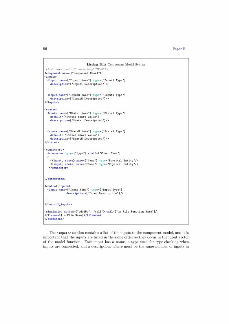
96 Paper B.
Listing B.1: Component Model Syntax
<?xml version="1.0" encoding="UTF-8"?>
<component name=["Component Name]">
<inputs>
<input name=["Input1 Name"] type=["Input1 Type"]
description=["Input1 Description"]/>
.
.
<input name=["InputN Name"] type=["InputN Type"]
description=["InputN Description"]/>
</inputs>
<states>
<state name=["State1 Name"] type=["State1 Type"]
default=["State1 Start Value"]
description=["State1 Description"]/>
.
.
<state name=["StateN Name"] type=["StateN Type"]
default=["StateN Start Value"]
description=["StateN Description"]/>
</states>
<connectors>
<connector type=["type"] conid=["Conn. Name"]
>
<{input, state} name=["Name"] type="Physical Entity"/>
<{input, state} name=["Name"] type="Physical Entity"/>
</connector>
.
.
</connectors>
<control_inputs>
<input name=["Input Name"] type=["Input Type"]
description=["Input Description"]/>
.
.
</control_inputs>
<simulation method={"ode15s", "call"} call=[".m File Function Name"]/>
<filename>[.m File Name]</filename>
</component>
The <inputs> section contains a list of the inputs to the component model, and it isimportant that the inputs are listed in the same order as they occur in the input vectorof the model function. Each input has a name, a type used for type-checking wheninputs are connected, and a description. There must be the same number of inputs in

2. Methods 97
the input list as the length of the input vector of the corresponding model function.The <states> section is similar to the input section except that it describes the states oroutputs of the function and that a default value must be declared. The default value isused as initial value in simulations when the simulation tool is not given an initial statevector to start from. Signals may be grouped together in connectors that allows theuser to connect a set of signals from one component model to a similar set on anothercomponent model in one operation.
Because this environment is used for refrigeration systems, it has a built-in con-nector class for refrigeration pipe interfaces but obviously, for other applications, otherconnections will be relevant - see Simulation Model Syntax in Subsection 2.2. On therefrigeration pipe interface three variables exist; a mass flow m, a pressure p, and an en-thalpy h. The model loader will return an error if each refrigeration pipe interface doesnot contain exactly one of each of the mentioned aforementioned types. The individualvariables may be either an input or a state but the model loader will check that each ofthe inputs can be connected to a state of the correct type when two refrigeration pipeinterfaces are connected. This saves the user the work of having to connect the variablesmanually, but when building the component models attention must be given to wherethe different states that are shared between models are located.

98 Paper B.
Simulation Model Syntax
The syntax for the simulation model XML file are shown in Listing B.2.
Listing B.2: Simulation Model Syntax
<?xml version="1.0" encoding="UTF-8"?>
<simulation_model name=["Simulation Model Name"]>
<component_path>[Component Library Path]
</component_path>
<components>
<component name=["Component Model Name"]
file=["Component Model XML File Name"]/>
.
.
<component name=["Component Model Name"]
file=["Component Model XML File Name"]/>
</components>
<connections>
<connector name=["Connector Name"]>
<component name=["Component Name"] conid=["Connection Name"]/>
<component name=["Component Name"] conid=["Connection Name"]/>
</connector>
<connection name=["Connection Name"]>
<component name=["Component Name"] type="Input" input=["Input Name"]/>
<component name=["Component Name"] type="Output" output=["Output Name"]/>
</connection>
</connections>
</simulation_model>
The simulation model is composed of a set of component models and their connec-tions described by the simulation model XML file, containing a list of the included compo-nent models and a description of how the components are connected. The <components>
section lists the component models used in the simulation model and it is allowed to usea component model more than once if they are given unique names. In the <connections>
section all the connections in the simulation model are listed. A connector connectionis established as in the <connector> sections by giving the name of the two componentmodels and the connector on each of the components. Inputs and outputs that are notassociated with connector interfaces, such as control inputs to actuators, are connectedin a <connection> section by listing the two components one by one. In each of the<component> sections it must be stated whether the signal is an input or an output, andwhat the name of the signal is. The model loader provides type checking on connectionsbetween components and gives a precise description, with the names of the implicated
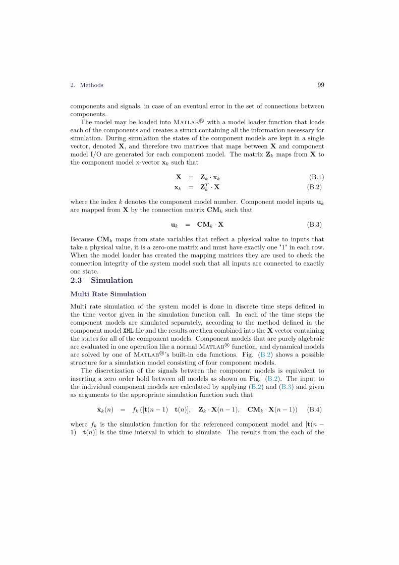
2. Methods 99
components and signals, in case of an eventual error in the set of connections betweencomponents.
The model may be loaded into MatlabR© with a model loader function that loads
each of the components and creates a struct containing all the information necessary forsimulation. During simulation the states of the component models are kept in a singlevector, denoted X, and therefore two matrices that maps between X and componentmodel I/O are generated for each component model. The matrix Zk maps from X tothe component model x-vector xk such that
X = Zk · xk (B.1)
xk = ZTk · X (B.2)
where the index k denotes the component model number. Component model inputs uk
are mapped from X by the connection matrix CMk such that
uk = CMk · X (B.3)
Because CMk maps from state variables that reflect a physical value to inputs thattake a physical value, it is a zero-one matrix and must have exactly one "1" in each row.When the model loader has created the mapping matrices they are used to check theconnection integrity of the system model such that all inputs are connected to exactlyone state.
2.3 Simulation
Multi Rate Simulation
Multi rate simulation of the system model is done in discrete time steps defined inthe time vector given in the simulation function call. In each of the time steps thecomponent models are simulated separately, according to the method defined in thecomponent model XML file and the results are then combined into the X vector containingthe states for all of the component models. Component models that are purely algebraicare evaluated in one operation like a normal Matlab
R© function, and dynamical modelsare solved by one of Matlab
R©’s built-in ode functions. Fig. (B.2) shows a possiblestructure for a simulation model consisting of four component models.
The discretization of the signals between the component models is equivalent toinserting a zero order hold between all models as shown on Fig. (B.2). The input tothe individual component models are calculated by applying (B.2) and (B.3) and givenas arguments to the appropriate simulation function such that
xk(n) = fk ([t(n − 1) t(n)], Zk · X(n − 1), CMk · X(n − 1)) (B.4)
where fk is the simulation function for the referenced component model and [t(n −1) t(n)] is the time interval in which to simulate. The results from the each of the

100 Paper B.
h
Fig. B.2: Example of a Simulation Model Structure
component simulations are then combined into the system state vector X by
X(n) =K
∑
k=1
Zk · xk(n) (B.5)
where K is the total number of components in the model. The simulation environmentmay then proceed and simulate the next time step with the same procedure as above.
Monolithic Simulation
In a monolithic simulation the entire collection of component models are lumped to-gether by a wrapper function and treated as a single model that may be simulated byode15s or another solver that accepts functions with a similar interface. This meansthat for every iteration of the solver all component functions are evaluated in order tofind a derivative for the entire collection of component models.
In [18] the multi-rate simulation speed of the reefer container system was comparedto the calculated speed for a monolithic simulation of the same system, showing thatthe modular approach was more than three times faster than the monolithic. There wasno comparison to an actual monolithic simulation of the system but by introducing amonolithic wrapper this is now possible.
The monolithic wrapper encapsulates the entire model into one function as shown onthe example in Figure B.3. The function simulate _model_monolithic() is used tosimulate the model by letting ode15s [20] simulate the wrapper for the desired period.Therefore the exact same component functions can be simulated as a monolithic blockwithout the need to combine them into one function or changing them in any way, giving

2. Methods 101
h
Fig. B.3: The monolithic wrapper
a lower probability for user errors. ode15s is as default set to use at least ten iterativesteps for each time period of the supplied time vector which in this case is 1000 stepsof one second, similar to the one used for the modular simulation.
In order to achieve a fair comparison to the modular simulation the monolithic solversmaximum step size is increased from the default 0.1s to 1s such that it can use multiplesteps if the dynamics require it, but also run faster if possible. The wrapper will forwardresults from the ODE and DAE components directly because their output is the statevector gradient, but for the algebraic functions the output is simply the new state atthe next sample point and therefore the gradient must be calculated and forwarded tothe solver. This is simply the difference between the new and the old state because thealgebraic functions of this model is designed for a sample time of one second.
Implications of using the ode15s solver
When calling the ode15s solver there is a considerable startup overhead and becausethe solver is called for each of the continuous components in every discrete time step thetotal time lost to this is large. According to [20] the ode15s solver relies on a Jacobianthat is generated automatically when it is not supplied by the user, as is the case inthis study. Because the calculation of the jacobian is requires a lot of computationsthe solver only generates the Jacobian when simulation is started, when the order andstep size is changed or if the solution is converging too slowly. Another drawback ofusing the solver in short steps is that it uses a very small step size in the beginning ofthe simulation period and then gradually increases it. Because the simulation periodis so short the solver never reaches larger step sizes and therefore it never reaches theefficiency expected of a variable time step solver, leading to a longer simulation time.
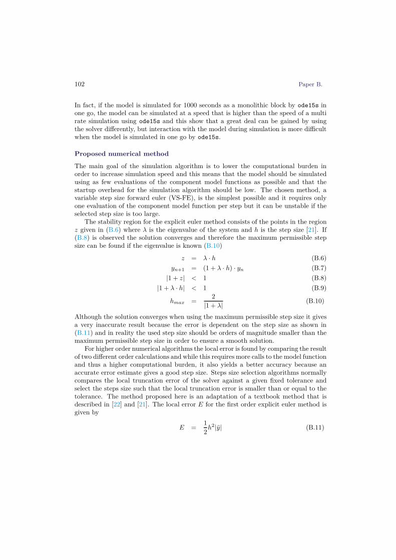
102 Paper B.
In fact, if the model is simulated for 1000 seconds as a monolithic block by ode15s inone go, the model can be simulated at a speed that is higher than the speed of a multirate simulation using ode15s and this show that a great deal can be gained by usingthe solver differently, but interaction with the model during simulation is more difficultwhen the model is simulated in one go by ode15s.
Proposed numerical method
The main goal of the simulation algorithm is to lower the computational burden inorder to increase simulation speed and this means that the model should be simulatedusing as few evaluations of the component model functions as possible and that thestartup overhead for the simulation algorithm should be low. The chosen method, avariable step size forward euler (VS-FE), is the simplest possible and it requires onlyone evaluation of the component model function per step but it can be unstable if theselected step size is too large.
The stability region for the explicit euler method consists of the points in the regionz given in (B.6) where λ is the eigenvalue of the system and h is the step size [21]. If(B.8) is observed the solution converges and therefore the maximum permissible stepsize can be found if the eigenvalue is known (B.10)
z = λ · h (B.6)
yn+1 = (1 + λ · h) · yn (B.7)
|1 + z| < 1 (B.8)
|1 + λ · h| < 1 (B.9)
hmax =2
|1 + λ|(B.10)
Although the solution converges when using the maximum permissible step size it givesa very inaccurate result because the error is dependent on the step size as shown in(B.11) and in reality the used step size should be orders of magnitude smaller than themaximum permissible step size in order to ensure a smooth solution.
For higher order numerical algorithms the local error is found by comparing the resultof two different order calculations and while this requires more calls to the model functionand thus a higher computational burden, it also yields a better accuracy because anaccurate error estimate gives a good step size. Steps size selection algorithms normallycompares the local truncation error of the solver against a given fixed tolerance andselect the steps size such that the local truncation error is smaller than or equal to thetolerance. The method proposed here is an adaptation of a textbook method that isdescribed in [22] and [21]. The local error E for the first order explicit euler method isgiven by
E =1
2h2|y| (B.11)

2. Methods 103
where h is the step size and y is the second order derivative of the state. SubstitutingE with the acceptable error local error tolerance T OL and isolating h yields the stepsize that limits how much the first order gradient is allowed to change in each step andtherefore also the magnitude of the local error
h =
√
2 · T OL
|y|(B.12)
where T OL is the absolute tolerance for the second order derivative of the system statethus bounding the step size with respect to how fast the first order derivative changesand thereby bounding the local error.
The different types of states in the container model are numerically very differentand therefore the second order derivative is also numerically very different. This meansthat if the step size is to be determined from the largest second order derivative givenby a model with multiple states the larger states will usually also have the larger secondorder derivative. The consequence of this is that states that are small may have arelatively large second order derivative but it will be ignored and that can result innumerical instability for states of small magnitude. For this model the notion of anabsolute error tolerance is therefore impractical and in order to address this problemthe second order derivative is normalized with respect to the size of the states as shownin (B.13).
ynorm =|y|
|y| + 1(B.13)
h =
√
2 · T OL
max(ynorm)(B.14)
h =
√
2 · T OL · (|y| + 1)
|y|(B.15)
Normalizing the second order derivative has a drawback: if a state approaches zerothe normalized second order derivative will approach infinity and result in very smallsteps. This issue is addressed by adding one to the state vector and therefore as a stateapproaches zero its normalized second order derivative will approach the real secondorder derivative. Due to the normalization of the second order derivative T OL is now ameasure of error relative to the state size for large states and it approaches a measure ofabsolute error as the states approach zero. For the solvers in the Matlab
R© ODE suitethe absolute and relative tolerances can be set independently [20], but that flexibility isnot needed for this application and therefore it is left out in order to have as simple asolver as possible.
In the remaining part of this section the proposed simulation algorithm and its stepsize calculation method is described and analyzed, starting with the Matlab
R© code
104 Paper B.
for the resulting simulation algorithm that is shown in Listing B.3. The algorithmshown above uses exactly one call of the model function for every step and because therest of the calculations are quite simple the function has a low overhead. In order toaccommodate the different experiments carried out in Section 2.4 it is possible to forcea fixed step size and limit the variable step size between a minimum and a maximum.Each step is started with an evaluation of the function that is being simulated in order toobtain the first order derivative. The second order derivative is then calculated from theold and the newly obtained first order derivatives and it is then normalized accordingto (B.13). Then the step size is calculated and limited and finally the step is takenwhereafter the sequence is repeated until the simulation reaches the end time. In thenext section the different experiments that are used to verify the performance of thesimulation environment and the solver is described.

2. Methods 105
Listing B.3: Proposed simulation algorithm
1 function [T, Y, error] = FESolver (fct_handle , t, y0, opts , u, p)23 N = (t(2) - t(1))/ opts.FE_minstep; % Maximum number of steps.45 T = zeros(1,N); % Time output vector6 Y = zeros(length (y0),N); % Solution output vector78 T(1) = t(1); % Set up initial values9 T_end = t(2);
10 Y(:,1) = y0;11 h = 1;12 y_dot_old = zeros(length(y0),1); % Assume zero gradient at beginning.
13 n = 1;14 error = 0;
15 while(T(n) < T_end)16 % Evaluate component function and obtain first order derivative.
17 y_dot = feval(fct_handle , T(n) , Y(:,n), u, p);18 % Calculate second order derivative from previously stored first19 % order derivative and step size.
20 y_dotdot = (y_dot - y_dot_old)/h;2122 if(opts.FE_Stepsize == 0)23 % Normalize the second order derivative with respect to the size of the24 % states, with one added in order to avoid high values for states near
25 % zero.26 norm_y_dotdot = abs(y_dotdot ) ./ (abs(Y(:,n)) + 1);
2728 % Use the largest change in gradient to calculate the step size.
29 h = sqrt(2*opts.FE_reltol / max(norm_y_dotdot));3031 % Limit the stepsize between min and max step size and ensure that it
32 % does not exceed the simulation end time.33 h = LimitValue(h, opts.FE_minstep , min(T_end - T(n), opts.FE_maxstep));
3435 else36 h = opts.FE_Stepsize; % For fixed step size.
37 end3839 % Update outputs40 T(n+1) = T(n) + h;
41 Y(:,n+1) = Y(:,n) + y_dot * h;42 y_dot_old = y_dot;43 % Check for faults and stop simulation on error
44 if(sum(isnan(y_dot)) > 0 || sum(abs(imag(y_dot ))) > 0)45 disp(’FESolver :␣Warning ␣NaN␣or␣IMAG␣returned ␣from␣simulation␣’)
46 error = 1;47 T(n+1) = T_end;48 end
49 n = n + 1;50 end
5152 % Only return the number of steps that was executed .
53 T = T(1:n);54 Y = Y(:,1:n);

106 Paper B.
2.4 Experiments
The required accuracy for the problem at hand is given by the objectives of the model;It must be adequate to do controller experiments and for the model to be used as anobserver for FDI in an embedded system. For the controller experiments it is importantthat the closed loop dynamical behavior of the system is accurate but because thecontrollers are designed to be robust to a rather large variance in the mechanical systemof the containers due to wear and tear and faulty or inadequate maintenance, a maxerror of 2% is acceptable. The average error is the normalized average error on all statesand the max error is the largest error on any of the states. The errors are calculatedfrom the states of all components except the controller because it will be replaced byan external controller when the model is moved to the embedded system.
When used as an observer for fault detection it is important that the faults are lowbecause a large uncertainty on the simulation result will require higher fault detectionthresholds to avoid false positives and thus the ability to detect small faults will belimited or the time to detect a fault will be too long. As an observer the model will berunning in open loop and therefore it is important that the long term static behavior isaccurate. It has been chosen to require that the max error on the variables importantfor control of the system stays below 5% for a three hour open loop simulation wherethe control inputs are recorded from a real container.
The proposed simulation method is tested in a variety of different scenarios on orderto qualify its performance and accuracy in the modes of operation where it is to be used.Furthermore a series of experiments are carried out to investigate the ode15s overheadand the nature of the reduction in accuracy caused by the proposed VS-FE method.Table B.1 shows a short list of the test carried out:
No. Description Solver1. Reference simulation - Fixed 1ms step monolithic FS-FE2. Reference simulation - Fixed 1ms step modular FS-FE3. Continuous monolithic ode15s
4. Stepwise monolithic ode15s
5. Modular ODE (previous method) ode15s
6. Modular variable step FE (new method) VS-FE7. Monolithic variable step FE VS-FE8. Open loop modular variable step FE VS-FE9. Open loop modular ODE ode15s
Table B.1: List of tests
Test 1 and 2: Reference simulations. In order to calculate the error of thedifferent experiments it is necessary to have a reference simulation that represents thetrue solution and this is achieved by simulating the model with a fixed step size that

2. Methods 107
is very small compared to the dynamics of the system. In this case a 1ms step size isfound to be adequate by simulating at both 1ms and 2ms step size and comparing theresults from which it was concluded that the error had converged. Two reference simu-lations are made; The first test is a monolithic simulation where the model is simulatedas one large block at 1ms resolution and that represents the true solution without theimpact from the ZOH of the modular simulation environment. The second reference isa modular simulation where the components are simulated independently with 1ms stepsize for one second at a time and the purpose is to isolate the error introduced by theZOH between the component models.
Test 3 and 4: Stepwise and Continuous monolithic ODE.In these two tests the model is simulated monolithically by the ode15s solver as a se-quence of one second steps and in one continuous go in order to identify the startupoverhead of the solver.
Test 5: Modular ODE (previous method).This is the simulation method presented in [18] and it is used as a baseline for verifica-tion of the new VS-FE solver.
Test 6: Modular variable step FE (new method).The VS-FE solver is compared to both reference simulations and to Test 5 in order toverify the performance of the simple solver in a modular environment.
Test 7: Monolithic variable step FE.It may be a viable option to simulate the model monolithically in order to avoid anyimplications from the modular simulation and therefore this test is carried out to verifythe speed and accuracy of this solution.
Test 8 and 9: Open loop modular VS-FE and ODE.In order to verify the long term stability and accuracy of the simulation environmentand the VS-FE solver is used to simulate the system in open loop over a three hourperiod with control signals recorded from a real container. The output of the modelon the measurements that are important for control of the system is then tested foraccuracy by comparing them to sensor measurements from the same real life data setas the control signals.
Test sequenceThe simulation model controller used in this experiment is programmed to ramp thecompressor speed 9 times during a 1000 second simulation in order to excite the systemand create some events that challenge the solver with large gradients on the systemstates. The modular simulation model that was presented in [18] was not excited as

108 Paper B.
much as in this test, leading to a low error due to the small gradients on the model states.When the system is excited more strongly the state gradients will be higher yielding alarger difference to the zero-gradient of the ZOH in the modular environment, whichgives a larger error.
3 Results
In this section the results of the tests carried out in Section 2.4 are listed and analyzedin order to identify viable options for simulating the model for controller experimentsand for use as an observer on an embedded system. The measured variables are thesimulation time, the average error and the max error. The average error is the nor-malized average error on all states and the max error is the largest error on any of thestates. The errors are calculated from the states of all components except the controllerbecause its states may go to zero and yield an infinite normalized error.On Figure B.4 the main results are shown and the references for calculating the errors
are the monolithic reference for the monolithic simulations and the modular referencefor the modular simulations. The error tolerance for the VS-FE method has been se-lected such that the error is approximately the same as produced by the ode15s solverwith standard tolerance settings [20] in order to make comparison of the results easier.From the results on Figure B.4 it can be seen that the simple VS-FE solver are able tooutperform the more advanced ode15s solver and in the following the reason for thiswill be analyzed.
Closed loop testsThe results of the relevant tests compared to the monolithic reference can be seen inTable B.2, where the time column is the time used simulating the 1000 second test andthe steps column has the number of steps used by the solver. For modular simulationsthe number of steps are the sum of steps used on the 9 components and for monolithicsimulations it is the number of times the monolithic wrapper function has been calledby the solver.
No Description Solver Time Mean Err. Max Err. Steps2. Modular Reference FS-FE 1458s 0.311% 1.615% 10000003. Cont. Monolithic ODE ode15s 35.6s 0.059% 0.447% 118784. Stepwise Monolithic ODE ode15s 399s 0.007% 0.029% 1269425. Modular ODE ode15s 37.2s 0.315% 1.654% 165626. Modular VS-FE VS-FE 11.3s 0.298% 1.499% 362887. Monolithic VS-FE VS-FE 9.89s 0.065% 0.273% 3970
Table B.2: Simulation results compared to the monolithic reference.

3. Results 109
0 0.5 1 1.5 2 2.5 3 3.5 4 4.5
2
3
4
5
6
Error wrt. Reference Simulation [%]Simulation time [s]
Tes
t num
ber
Monolithic Stepwise ODE412.0s
0.06%0.01%
Monolithic Continuous ODE28.6s
0.71%0.10%
Monolithic Variable Step FE − (Proposed Method)15.3s
0.49%0.10%
Modular Stepwise ODE − (Previous Method)54.6s
3.00%0.46%
Modular Variable Step FE − (Proposed Method)15.6s
2.79%0.42%
Simulation timeMax errorMean error
Fig. B.4: Comparison of test results for monolithic and modular methods.
The error for Test 2 - Modular reference shows the magnitude of the error introducedfrom the multi-rate simulation itself and it is a consequence of the ZOH delays betweencomponent models. Therefore this error is also large when gradients are as large as theyare in this test, due to the high excitation of the model. In a controller experimentsetup the ZOH delays are not critical because they are small compared to the dynamicsthat are important for control which according to [23] for a refrigeration system arethe thermal masses of the evaporator and the condenser. Under normal operation therefrigeration system is in steady state most of the time and therefore the temporalinaccuracy during steep gradients imposed by the ZOH delays has little impact on theaccuracy of long term simulations.

110 Paper B.
0 100 200 300 400 500 600 700 800 900 10000
10
20
30
Sim
ulat
ion
Ste
psSimulation Profile for: "Test 5: Modular Stepwise ODE"
boxevapcprcondrecvsjecon
0 100 200 300 400 500 600 700 800 900 10000
50
100
Sim
ulat
ion
Tim
e [m
s]
boxevapcprcondrecvsjecon
0 100 200 300 400 500 600 700 800 900 10000
10
20
30
Time Step
Sim
ulat
ion
Tim
e / S
tep
[ms]
boxevapcprcondrecvsjecon
Fig. B.5: Simulation profile for the modular simulation with the ode15s solver.
Test 3 - Continuous Monolithic ODE and 4 - Stepwise Monolithic ODE illustratesthe importance of using the ode15s solver as it is intended to be used, which is visiblethrough the large difference in simulation time. Test 3 simulates the model in onego, that is the solver controls the simulation from start to end and can run withoutinterruptions. In Test 4 the solver simulates one second at a time, and therefore it hasto linearize the model before every step and it is only able to step 1s forward. Thiscauses it to use more than ten times as many calls to the monolithic wrapper as is usedby the solver in Test 3, resulting in a very inefficient solution of the problem.
The results for the old method [18] running on this test sequence is shown in Test5 - Modular ODE and it can be seen that the error is a bit higher than the error forTest 2 which indicates that the ode15s does a good job. The simulation profile thatshow the number of steps and time consumed for each of the components in this testare shown on Figure B.5.
The simple solver show an unexpected result in Test 6 - Modular VS-FE, it has ashorter simulation time than the old method but it still manages to produce a smaller
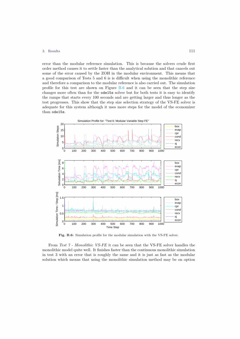
3. Results 111
error than the modular reference simulation. This is because the solvers crude firstorder method causes it to settle faster than the analytical solution and that cancels outsome of the error caused by the ZOH in the modular environment. This means thata good comparison of Tests 5 and 6 is is difficult when using the monolithic referenceand therefore a comparison to the modular reference is also carried out. The simulationprofile for this test are shown on Figure B.6 and it can be seen that the step sizechanges more often than for the ode15s solver but for both tests it is easy to identifythe ramps that starts every 100 seconds and are getting larger and thus longer as thetest progresses. This show that the step size selection strategy of the VS-FE solver isadequate for this system although it uses more steps for the model of the economizerthan ode15s.
0 100 200 300 400 500 600 700 800 900 10000
5
10
15
20
Sim
ulat
ion
Ste
ps
Simulation Profile for: "Test 6: Modular Variable Step FE"
boxevapcprcondrecvsjecon
0 100 200 300 400 500 600 700 800 900 10000
2
4
6
8
Sim
ulat
ion
Tim
e [m
s]
boxevapcprcondrecvsjecon
0 100 200 300 400 500 600 700 800 900 10000
0.5
1
1.5
Time Step
Sim
ulat
ion
Tim
e / S
tep
[ms]
boxevapcprcondrecvsjecon
Fig. B.6: Simulation profile for the modular simulation with the VS-FE solver.
From Test 7 - Monolithic VS-FE it can be seen that the VS-FE solver handles themonolithic model quite well. It finishes faster than the continuous monolithic simulationin test 3 with an error that is roughly the same and it is just as fast as the modularsolution which means that using the monolithic simulation method may be on option

112 Paper B.
when there is a need for high accuracy.Because of the large error from the modular simulators ZOH it is difficult to verify the
performance of test 5 and 6 and they are therefore compared to the modular reference,with the results shown in Table B.3. from the results it is clear that the VS-FE solver
No Description Solver Time Mean Err. Max Err. Steps5. Modular ODE ode15s 54.6s 0.021% 0.213% 152476. Modular VS-FE VS-FE 15.6s 0.032% 0.190% 34072
Table B.3: Simulation results compared to the modular reference.
are capable of simulating this system with the same accuracy as the ode15s solver 3.5times faster, even though it needs twice the amount of steps to do it. The ode15s solveruses approximately 3.75ms per step due to the solvers startup overhead and because theVS-FE solver uses only 0.455ms per step and has almost no startup overhead its speedadvantage increases if the error tolerance of the two solvers are increased. Therefore theVS-FE solver is a better choice for a solver in the modular configuration.
Open loop testsThe test sequence in Tests 1 to 7 are designed to show dynamical errors that are relevantwhen doing controller experiments but they do not verify the long term stability of thesimulation environment and the model. Long term stability and accuracy are two veryimportant parameters for a simulation model and this is verified with an open loop testthat simulates the system model without feedback control for three hours. The initialstate for the model is set to match the initial state for a real container and the model isthen simulated with the sampled control signals from the refrigeration container. Fivemeasurements that are characteristic for the system are then compared to the result ofthe simulation in order to verify that the model is stable for longer runs and that theVS-FE solver does not compromise the accuracy of the solution. In Table B.4 the resultsof these two tests are shown. Tret and Tsup are the return and supply air temperatures
No Solver Time Tret Tsup Tsuc Pdis Psuc8. Modular ODE 622s 0.541% 0.957% 0.790% 2.183% 1.369%9. Modular VS-FE 97.6s 0.545% 0.954% 0.795% 2.183% 1.369%
Table B.4: Open loop simulation results.
for the container, respectively and they are important for the temperature control andestimation of actual cooling capacity. The suction temperature Tsuc is the temperatureof the refrigerant vapor going from the evaporator to the compressor and combined withthe suction pressure Psuc it forms the control signal for control of the evaporator. Thelast signal Pdis is the discharge pressure of the compressor. With feedback from these
4. Conclusion 113
five signals it is possible to control the refrigeration system. As it can be seen, the errorof the two simulations are almost identical but the VS-FE solver is six times faster thanthe previous method that use the ode15s solver and therefore the obvious choice for asolver in an observer is the VS-FE method.
4 Conclusion
A modular simulation environment was presented with a dynamical model of a refrig-eration container. Different options for simulating the model for controller experimentsor as a full system observer to be used in the embedded controller for the refrigerationcontainer was tested and analyzed. It was demonstrated that the variable step forwardeuler modular simulation approach may be used to simulate vapor compression cycleswithout the loss of accuracy but with a significant increase in speed. The impact ofsimulating a model of a refrigeration system with the multi-rate method has been ana-lyzed with respect to dynamical and static errors and it was shown that the multi-ratemethod combined with the variable step forward euler solver was the best option for anembedded observer. A comparison between monolithic and multi-rate simulations onthe same model was done and showed that the variable step forward euler solver wasfaster than the ode15s solver in both scenarios without increasing the error. From thetests it can be concluded that it is very important to use a solver with low overhead in amulti-rate environment because simulation times are short and therefore a an advancedsolver never reaches its true potential. Design and simulation of reefer systems based ona modular simulation concept have shown very promising results. Simulation speed hasbeen increased by up to 350% and it has been shown that the trade-off - inaccuracy - hasno real impact on results. The simulation environment and the model have been verifiedto be more accurate than necessary for control experiments and therefore a decrease insimulator accuracy is acceptable when modular simulation is used.
114 References
References
[1] D. S. C. Limited, “Reefer shipping market annual report,” Drewry House, 213Marsh Wall, London, E14 9FJ,England, 2009. [Online]. Available: http://www.drewry.co.uk/get_file.php?id=1161
[2] M. Blanke, M. Kinnaert, J. Lunze, and M. Staroswiecki, Diagnosis andFault-Tolerant Control. Springer, 2003.
[3] “Container haandbook, cargo loss prevention information from german marineinsurers.” [Online]. Available: http://www.containerhandbuch.de/chb_e/wild/index.html?/chb_e/wild/wild_08_01_02.html
[4] MCI, “Maersk container industry, starcool refrigerated container specifications,”2013. [Online]. Available: http://www.maerskbox.com/
[5] L. S. Larsen, C. Thybo, and H. Rasmussen, “Intelligent control - optimizing theoperation of refrigeration systems under daily variations in ambient temperature,”in Danske Køledage, March 15th-16th, 2007. Proceedings of Danske Køledage2007., 2007.
[6] J. Cai, J. Stoustrup, and J. Jorgensen, “Preventing refrigerated foodstuffs insupermarkets from being discarded on hot days by mpc,” in Proceedings of the17th IFAC World Congress, Seoul, Korea, 2008. [Online]. Available: http://www.control.aau.dk/~jakob/selPubl/papers2008/ifacwc_2008_3.pdf.doi:10.3182/20080706-5-KR-1001.01880
[7] “Trnsys.” [Online]. Available: http://sel.me.wisc.edu/trnsys/
[8] “Dymola.” [Online]. Available: http://www.dynasim.se/index.htm
[9] P. Fritzson and P. Bunus, “Modelica – a general object-oriented language forcontinuous and discrete-event system modeling,” in IN PROCEEDINGS OF THE35TH ANNUAL SIMULATION SYMPOSIUM, 2002, pp. 14–18.
[10] M. Skovrup, “Windali - an open-structured component modeling and simulationprogram based on standard programming languages,” in Proceedings of SIMSConference. Lyngby, 2000, pp. 157–172.
[11] “MatlabR© Simulink
R©.” [Online]. Available: http://www.mathworks.com/products/simulink/
[12] Z. Yang, K. Rasmussen, A. Kieu, and R. Izadi-Zamanabadi, “Fault detection andisolation for a supermarket refrigeration system - part two,” Proceedings of the18th IFAC World Congress, 2011, pp. 4238–4243, 2011, iFAC Workshop Series2011.

References 115
[13] R. Kübler and W. Schiehlen, “Modular simulation in multibody systems,”Multibody System Dynamics, vol. 4, pp. 107–127, 2000.doi:10.1023/A:1009810318420
[14] C. Rosen, D. Vrecko, K. Gernaey, and U. Jeppsson, “Implementing adm1 forbenchmark simulations in matlab/simulink,” Journal of Water science andtechnology, vol. 54, no. 4, pp. 11–19, 2006. doi:10.2166/wst.2006.521
[15] Guo-liang Ding, “Recent developments in simulation techniques forvapour-compression refrigeration systems,” International Journal of Refrigeration,vol. 30, no. 7, pp. 1119–1133, 2007. doi:10.1016/j.ijrefrig.2007.02.001
[16] R. M. Howe, “Accuracy and stability tradeoffs in multirate simulation,” inProceedings of SPIE, vol. 4367, 2001, pp. 113–126. doi:10.1117/12.440011
[17] J. G. Pearce, R. E. Crosbie, J. J. Zenor, R. Bednar, D. Word, and N. G.Hingorani, “Developments and applications of multi-rate simulation.” in UKSim,D. Al-Dabass, Ed. IEEE, 2009, pp. 129–133. [Online]. Available: http://dblp.uni-trier.de/db/conf/uksim/uksim2009.html#PearceCZBWH09.doi:10.1109/UKSIM.2009.23
[18] K. Sørensen and J. Stoustrup, “Modular modelling and simulation approach -applied to refrigeration systems,” in Proceedings of IEEE InternationalConference on Control Applications, San Antonio, Texas, USA, September 2008,pp. 983 – 988. doi:10.1109/CCA.2008.4629691
[19] K. Sørensen, M. Skovrup, L. Jessen, and J. Stoustrup, “Modular modelling of areefer container,” Submitted for publication, 2013.
[20] L. F. Shampine and M. W. Reichelt, “The matlab ode suite,” Journal onScientific Computing, vol. 18, pp. 1–22, 1997. doi:10.1137/S1064827594276424
[21] J. C. Butcher, Numerical methods for ordinary differential equations. J. Wiley,2003. [Online]. Available: http://www.worldcat.org/isbn/9780471967583
[22] E. Kreyszig, Advanced Engineering Mathematics, 9th ed. Wiley, Nov. 2005.[Online]. Available: http://www.amazon.com/exec/obidos/redirect?tag=citeulike07-20&path=ASIN/0471488852
[23] B. Rasmussen, A. Musser, and A. Alleyne, “Model-driven system identification oftranscritical vapor compression systems,” IEEE Transactions on Control SystemsTechnology, vol. 13, no. 3, pp. 444–451, 2005. doi:10.1109/TCST.2004.839572

116 References

Paper C
Modular Modeling of a Refrigerated Container
Kresten K. Sørensen, Lars M. Jessen, Morten Juel Skovrup, Jakob
Stoustrup
Submitted to: International Journal of Refrigeration, November 2013.

Copyright c© 2013 Elsevier Ltd and the International Institute of Refrigeration (IIR).All rights reservedThe layout has been revised.

119
Abstract
This paper presents the modeling of a refrigeration container for use as a reference forenergy-optimizing controller design. The model is based on first principles in order toconserve mass and energy, but various assumptions are used to simplify the equations,resulting in a unified model for the Star Cool refrigeration unit, the container and thecargo. Comparisons between simulations using the model and measurements from a realcontainer show an average error of less than ±1K on the states important for control.
Nomenclature
Latin symbolsM Mass (kg)m Mass flow (kg/s)Q Energy flow (W)V Volume (m3)v Specific Volume (m3/kg)h Specific enthalpy (J/kg)p Pressure (Bar)T Temperature (C◦)X Refrigerant Quality (kg/kg)c Specific heat (J/(Kg K))UA Overall heat transfer coefficient (W/K)s Second
Greek symbols∆ Property variationγ Heat capacity ratioK Expansion device characteristic constantλ Pressure drop ratio (Bar s/kg)ω Compressor Speed (Hz)σ Control volume boundaryρ Density (kg/m3)
Subscriptsa Airm Metalamb Ambientc CargoCp Constant pressureCv Constant volumef FloorC Clearancei Control volume, il Liquidv Vaporr Refrigerantsc Sub-cooledaa Ambient to airaf Ambient to floorca Cargo to airret Return air from cargosup Supply air to cargoamv Air to metal around vapor volumeaml Air to metal around liquid volumefa Floor to air

120 Paper C.
1 Introduction
Modern control theory is a discipline in which controllers are designed from mathemati-cal models of the dynamical systems that they are intended to control. The performanceof the controller relies on good system models, and therefore, the modeling of the systemshould receive as much attention as designing the controller itself. Another importantapplication of system models is simulations, in which a computer is used to simulate thebehavior of a real system. Numerical simulations are extensively used for experimentswithin the field of control engineering, and with the increasing power of computers,faster than real time simulations of very large dynamical systems have become possibleusing ordinary desktop PCs. The model presented in this paper is constructed for themodular simulation environment presented in [1, 2].
A refrigeration container is an insulated container with an integrated refrigerationunit that is used for the international transport of different types of chilled or frozenfoods. Good controller performance is essential for these systems if both high foodquality and energy efficiency are to be achieved [3]; consequently, a good model isrequired. The subject of refrigeration plant modeling is well covered for industrialand HVAC systems, but the modeling of refrigeration containers is only covered in afew works [4, 5, 6], which primarily focus on product quality control of chilled foods.Chilled foods generally ripen in the container and that must be controlled if the cargois to survive the trip, and therefore, the focus of these models is the cargo dynamicsand not the refrigeration plant itself. It has been shown by [7, 3] that a significantamount of energy can be saved by adapting to daily variations in ambient temperatureusing a Model Predictive Controller (MPC). To enable simulation experiments usingthis technology, a detailed model of the refrigeration plant and container is needed.
The objective of the present was to develop a model that captures the dynamicsrequired to test and design an energy-optimizing controller for a refrigeration container.The requirements for such a model are that the static and dynamic behaviors shouldsufficiently match those of the real system to be used for closed-loop control experimentsand that the simulations should run at least one order of magnitude faster than experi-ments on the real system. Another important requirement is that it must be possible tochange the model configuration without having to rewrite or reorganize the entire set ofequations for the model by hand. Therefore, a modular approach is selected, in whichthe model of the refrigeration system is composed of a set of interchangeable componentmodels that are based on a mix of first principles and assumptions. First principles aresubstituted by assumptions where it has a positive effect on simulation speed and asmall effect on model accuracy.
We present a simulation model of a refrigeration container that focuses on the dyna-mics that are important from a control perspective. The presented model is nonlinearto properly reflect the static performance of the system under different operating condi-tions, and it is primarily used as a tool for testing and validating controllers; however,

2. Modeling 121
linear models derived from the nonlinear simulation model are also used for controllerdesign. The container modeled in this paper is constructed by Maersk Container Indus-try (MCI) and is equipped with a Star Cool refrigeration unit. This unit possesses someunique properties that make it an obvious target for advanced control. The compressoris controlled by a Variable Frequency Drive (VFD) that allows the compressor speed tobe adjusted from 20Hz to 110Hz and electronic expansion valves that can be controlledfrom 0% to 100%. The fact that the control inputs can be controlled independentlymeans that a certain cooling power can be achieved with a range of different controlset-point combinations. However, not all combinations of set-points are equally efficient,and therefore, it is important that the model is able to reflect the overall efficiency ofthe system such that an energy-optimizing controller can be designed from the model.
2 Modeling
The container consists of a large insulated box with a refrigeration unit at one endand a loading door at the other. The refrigeration unit cools and circulates cold airaround the cargo, as depicted in Figure C.1. The cold air is injected into the floor ofthe container by the evaporator fans and travels below the cargo to the far end of thecontainer. The air heats up as it rises between the cargo and along the walls to the topof the container, where the air flows back to the refrigeration unit. A schematic of therefrigeration system is presented in Figure C.2.
Fig. C.1: Airflow in the Refrigeration Container
The refrigeration system consists of a two-stage piston compressor, a condenser, anevaporator, two expansion valves, three fans and an economizer. The economizer is acounter-flow plate heat exchanger used to increase the capacity of the system when thereare high temperature differences between the cold and hot sides. The expansion valves

122 Paper C.
are electromagnetically pulsed on/off valves, and the fans may run at half or full speedor be turned off completely. There are three major pressure levels in this setup: p1 isthe evaporator pressure, p2 is the intermediate pressure between the two compressorstages, and p3 is the condenser pressure.
Fig. C.2: Refrigeration System for a Refrigeration Container
The objective of the model of the refrigeration container is to capture the dynamicsthat are important to the temperature inside the box to create a model-based controllerfor the container. Additionally, for future studies, it is desired to be able to track themovement of the refrigerant charge in the system to enable experiments aiming to reducethe overall refrigerant charge needed.
According to [8], the salient dynamics of a refrigeration system are the thermaltime constants of the metal surfaces in the heat exchangers. Furthermore, accordingto [8], some components have dynamics that are so fast compared to the dominantdynamics that they may be replaced with algebraic equations, thereby reducing themodel order while preserving the physical behavior of the model. The components thatmay be modeled algebraically are the expansion valves and the compressor [9], whilethe remainder of the components are modeled using a mix of differential and algebraicequations. The resulting model is a dynamical model of the thermal masses in the heatexchangers, the cargo and the metal in the cargo hold with a model of the refrigerationcycle that includes the mass balances for the refrigerant in each control volume but withsteady-state equations for the momentum and energy balances [10]. The disadvantage ofthis approach is that some dynamics are missing, but the advantage is that the resultingsystem is less stiff, which results in a higher simulation speed [11].
The model is composed of a set of component models, where each model correspondsto a physical component in the refrigeration system. The state in each control volume isgiven by pressure and enthalpy. Pressure is used to balance the exchange of refrigerantflow between component models, and therefore, two connected components must haveaccess to the pressure of the other component. Refrigerant conversion calculations are

2. Modeling 123
performed using the WinDali [12] refrigeration equation toolbox for MatlabR©.
A typical set of state equations for a control volume containing refrigerant wouldthen be
dM
dt= min − mout (C.1)
hout = hin +Qin
min
(C.2)
Equation (C.1) is the mass balance, where the change in mass dMdt
is the net mass flowinto the volume given by the difference between min and mout. Equation (C.2) is theenergy balance.
In most cases, the interface between the component models is the pipes carryingrefrigerant, and such an interface has three states: pressure, mass flow and specificenthalpy. Zero-order-holds are inserted between the component models by the modularsimulation environment [1, 2], and therefore, changes in the states in one componentare not effective in the other components until the next step in the simulation.
This means that the dynamics of the states on the interfaces should be slow comparedto the sampling time of the simulation environment to avoid simulation instability andimprecise results.
The refrigeration system has some very fast, pulsating, pressure dynamics around thecompressor, which are not interesting from a control perspective. The primary objectiveof the control algorithm is to keep the supply air temperature steady; therefore, fastdynamics that have little influence on the supply air temperature can be neglected. Toavoid modeling fast pressure transients, it was decided to place the pressure equationsin the components with the slowest dynamics. Therefore, at the interface between theevaporator and the compressor, the pressure is modeled by the evaporator and the massflow is modeled by the compressor.
Two pipe junction models are required to model the joining and splitting of refriger-ant flows that occur between the compressor stages and after the receiver, respectively.
2.1 Pipe Joining Junction
The pipe joining junction model is located between the two compressor stages and theeconomizer and joins the mass flows from the first compressor stage and the economizerinto one mass flow that is fed to the second compressor stage. This model includes theinternal volume of the compressor and has two states, refrigerant mass M and outputenthalpy hout, and five inputs, which are the mass flows on all three interfaces min1,min2, and mout and the input enthalpy for both refrigerant inputs hin1 and hin2. The

124 Paper C.
governing equations of the model are
dM
dt= min1 + min2 − mout (C.3)
hout =hin1 · min1 + hin2 · min2
min1 + min2(C.4)
The change in internal mass is modeled by Equation (C.3) as the net sum of themass flow on the three interfaces. Equation (C.4) is the energy balance, where it isassumed that no heat transfer to the surroundings occurs.
2.2 Pipe Splitting Junction
The splitting junction is located between the receiver and the economizer, and the modelis very simple because it is only a division of one mass flow into two. The pressure andenthalpy on the outputs are equal to the input pressure and enthalpy, and the massflows on the inputs are equal to the sum of the mass flows on the two outputs. Becausethere are no slow internal dynamics, this model is implemented as an algebraic function.The equations for this component are as follows:
min = mout1 + mout2 (C.5)
pout1 = pin (C.6)
pout2 = pin (C.7)
hout1 = hin (C.8)
hout2 = hin (C.9)
2.3 Compressor
The compressor has two almost identical stages, in which the only difference is thatthe displacement volume of the first stage is twice as large as that of the second stage;therefore, only the equations for one stage are shown here. The compressor stages aremodeled by two algebraic functions that give the mass flow m and output enthalpyhout as a function of the input and output pressures pin and pout, the input enthalpyhin and the speed of the compressor ω. The physical behavior in the model includesadiabatic compression, clearance volume, and valve pressure loss. The dynamics causedby the piston strokes are decoupled from the slower evaporator dynamics because asingle piston stroke has a very small impact on the evaporator temperature. Therefore,the dynamics from the pulsating pressure caused by the piston strokes can be neglectedand substituted with an algebraic model in which the mass flows on the input andoutput are equal. The model calculates the mass displaced in a single stroke from thedensity of the incoming refrigerant vapor and the clearance volume, and then the mass

2. Modeling 125
is scaled with the compressor speed. The pressures p1 and p2 are the actual input andoutput pressures at the piston and are calculated from the valve loss as
p1 = pin − kl1 · ω (C.10)
p2 = pout + kl2 · ω (C.11)
where ω is the compressor speed and kl is the valve loss constant. The subscript 1 isused for variables calculated on the basis of pin, and the subscript 2 is used for variablescalculated on the basis of pout. Assuming an adiabatic compression, the mass flow andoutput enthalpy can be calculated as
γ = Ccp/Ccv (C.12)
v2 =
(
p2
p1
)
−1
γ
· v1 (C.13)
m =
(
V1
v1−
VC
v2
)
·ω
2(C.14)
Tout = Tin ·
(
pout
pin
)
γ−1
γ
(C.15)
hout = HT P (Tout, pout) (C.16)
Equation (C.12) yields the ratio γ between the specific heat of the refrigerants at con-stant pressure Ccp and constant volume Ccv. In Equation (C.13), the specific volume ofthe refrigerant at the discharge pressure p2 is calculated, assuming adiabatic compres-sion, from the specific volume v1 and pressure of the input refrigerant p1. In Equation(C.14), V1 and v1 are the internal volume of the cylinder and the specific volume ofthe refrigerant before the stroke, respectively; VC is the clearance volume and thus theinternal cylinder volume after the stroke; and v2 is the specific volume of the refrigerantafter the stroke. The mass displaced in a single stroke is the difference between the massof the gas in the cylinder with the piston in either extremity, and this is multiplied bythe compressor speed to obtain the mass flow. The output temperature Tout is givenby Equation (C.15) and is used to find the output enthalpy in Equation (C.16) by tablelookup [13].
2.4 Condenser
The condenser models the discharge pressure of the refrigeration system, and the accu-racy of this state is important because the energy consumption of the compressor andthe mass flow through the expansion valves are dependent on the discharge pressure.In [8], it is shown that the dominant dynamics in the condenser are determined by thetemperature of the metal, and therefore, a simple model with a single refrigerant controlvolume is used.
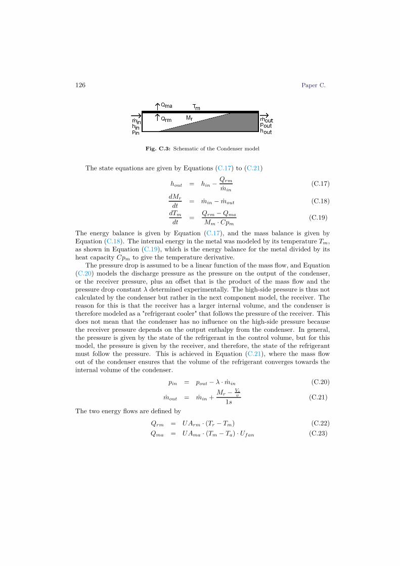
126 Paper C.
Fig. C.3: Schematic of the Condenser model
The state equations are given by Equations (C.17) to (C.21)
hout = hin −Qrm
min
(C.17)
dMr
dt= min − mout (C.18)
dTm
dt=
Qrm − Qma
Mm · Cpm
(C.19)
The energy balance is given by Equation (C.17), and the mass balance is given byEquation (C.18). The internal energy in the metal was modeled by its temperature Tm,as shown in Equation (C.19), which is the energy balance for the metal divided by itsheat capacity Cpm to give the temperature derivative.
The pressure drop is assumed to be a linear function of the mass flow, and Equation(C.20) models the discharge pressure as the pressure on the output of the condenser,or the receiver pressure, plus an offset that is the product of the mass flow and thepressure drop constant λ determined experimentally. The high-side pressure is thus notcalculated by the condenser but rather in the next component model, the receiver. Thereason for this is that the receiver has a larger internal volume, and the condenser istherefore modeled as a "refrigerant cooler" that follows the pressure of the receiver. Thisdoes not mean that the condenser has no influence on the high-side pressure becausethe receiver pressure depends on the output enthalpy from the condenser. In general,the pressure is given by the state of the refrigerant in the control volume, but for thismodel, the pressure is given by the receiver, and therefore, the state of the refrigerantmust follow the pressure. This is achieved in Equation (C.21), where the mass flowout of the condenser ensures that the volume of the refrigerant converges towards theinternal volume of the condenser.
pin = pout − λ · min (C.20)
mout = min +Mr − Vi
v
1s(C.21)
The two energy flows are defined by
Qrm = UArm · (Tr − Tm) (C.22)
Qma = UAma · (Tm − Ta) · Ufan (C.23)

2. Modeling 127
where Qrm is the flow from refrigerant to metal and Qma is the flow from metal to air.Tm is the temperature of the metal, and Ta is the temperature of the air that is blownover the condenser coil by the fan. Tr is the refrigerant temperature at the output of thecondenser calculated from pout and hout, under the assumption that the heat transferis independent of the refrigerant mass flow. It is assumed that the energy flow from themetal to the air is linearly dependent on the airflow, and therefore, the energy flow ismultiplied by the speed of the condenser fan, which is denoted Ufan. The fan speedcan have the values of 0.05, 1 and 2, which correspond to stopped, low speed and highspeed, respectively. When the fan is stopped, some natural convection still exists, andthis is modeled by assuming a fan speed of 0.05 when the fan is off. The value wasfound to be the best match for the data used to verify the model, but the amount ofconvection when the fan is off is expected to vary depending on the wind conditions.
The heat transfer coefficients UArm and UAma determine the steady-state condens-ing pressure, and they were found in a steady-state experiment on a special test unitequipped with extra temperature and pressure sensors. The mass flow of refrigerant wascalculated from the compressor speed and suction pressure, using manufacturer data forthe compressor. This was used to calculate the heat flux from the refrigerant to themetal, which in steady state is equal to the heat flux from the metal to the air. Us-ing the air, metal and refrigerant temperatures, the heat transfer coefficients were thencalculated to be 650 J/K for UAma and 1500 J/K for UArm. The same method wasapplied when the UA values for the heat transfers between metal, air and refrigerantwere found for the evaporator.
2.5 Receiver
The receiver is a buffer tank for excess refrigerant; the refrigerant is led from the con-denser into the top of the receiver, and liquid refrigerant to the expansion valves istaken from the bottom. The receiver is generally either neglected in dynamical modelsof refrigeration plants or not existent in the modeled plant, but the receiver is, however,not entirely without influence on the refrigeration systems dynamics, particularly duringrapid pressure changes [14]. The reason for this is that the liquid in the receiver actsas a buffer and has a dampening effect on pressure transients from the condenser andrefrigerant temperature transients on the input of the expansion valves. The liquid inthe receiver that flows to the expansion valves may be either sub-cooled or at the boilingpoint, and if the liquid starts to boil, it will turn into a two-phase mixture of liquid andvapor with a quality that depends on the size of the pressure drop. When the condenserfan is turned on, the pressure in the receiver can drop rapidly, and if the temperatureof the liquid in the receiver is close to the boiling point, it will begin to boil until therefrigerant temperature drops below the boiling point or the pressure increases abovethe bubble point. The liquid boiling into vapor counteracts the pressure drop, and thehybrid [15] behavior caused by this is included in the model.

128 Paper C.
The receiver has two control volumes, one with vapor and one with liquid, and eachof these volumes has four possible sets of equations that are determined by the qualityof the refrigerant entering the control volumes and the quality of the refrigerant in thecontrol volume itself. The input refrigerant is divided between the liquid and vaporcontrol volumes when the refrigerant entering the receiver has a quality above zero andto the liquid control volume only when the quality of the input refrigerant is less thanor equal to zero. Figure C.4 presents a schematic of the mass and heat flows modeledin the receiver.
Fig. C.4: Schematic of the Receiver
The inputs of the model are the input mass flow min, the input enthalpy of therefrigerant coming from the condenser hin and the mass flow of the refrigerant leavingthe receiver mout. The states of the model are the pressure p, the enthalpy of the liquidcontrol volume hl, the enthalpy of the vapor control volume hv, the mass of refrigerantin the liquid volume ml and the mass of refrigerant in the vapor volume mv.
The hybrid behaviour related to the input refrigerant is given by Equations (C.24)to (C.27).
mlin = min · (1 − Xin)∣
∣
Xin=[0,1](C.24)
mvin = min · Xin
∣
∣
Xin=[0,1](C.25)
Equations (C.24) and (C.25) show the mass flows into the two control volumes ofthe receiver, which are the input mass flow split by the void fraction of the refrigerant.
The enthalpy of the refrigerant that flows from the condenser to the two receiver

2. Modeling 129
control volumes are given by Equations (C.26) and (C.27):
hvin = HDewP (pin) (C.26)
hlin =
{
HBubP (pin) if Xin > 0;
hin otherwise.(C.27)
The vapor entering the vapor volume, hvin, is modeled as being at the dew point,under the assumption that the condenser always manages to condense at least a fractionof the refrigerant. The mass flow into the liquid control volume, mlin, may be either atthe bubble point or sub-cooled depending on the performance of the condenser.
The mass flow from the liquid volume to the vapor volume, mblv, is positive whenthe liquid is boiling and otherwise zero, as given by:
mblv =
{
Xl · Ml if hl > HBubP (p);
0 otherwise.(C.28)
It is assumed that the mass flow between the two control volumes is instant andtherefore equal to the product of the fraction of vapor or liquid and the mass of refriger-ant in the control volume. The following equation models the mass flow from the vaporvolume to the liquid volume, given by condensation in the vapor volume.
mcvl =
{
(1 − Xv) · Mv if hv < HDewP (p);
0 otherwise.(C.29)
The two control volumes are thermally connected through the surface of the liquidvolume and through the metal housing of the receiver. The resulting heat flow is givenby Equation (C.30):
Qvl = UA · (Tv − Tl) (C.30)
The equations for mass and energy balances are given by Equations (C.31) to (C.34):
hl = hlin +Qvl
mlin
(C.31)
hv = hvin −Qvl
mvin
(C.32)
dMl
dt= mlin + mvl − mout (C.33)
dMv
dt= mvin − mvl (C.34)

130 Paper C.
where mvl is the flow of refrigerant from the vapor volume to the liquid volume givenby the difference between mcvl and mblv
mvl = mcvl − mblv (C.35)
2.6 Expansion Valve
It is important for the mass flow given by the expansion valve model to be accuratebecause the mass flow is one of the determining factors for the cooling capacity of thesystem. According to [16], the expansion process can be considered adiabatic due to thevery small internal volume of the expansion valve. Therefore, the expansion valve modelis purely algebraic and modeled as a continuous valve that gives the average mass flowof the electromagnetically pulsed on/off valves used in the container. The continuousmodel was chosen because the pressure transients on the suction side of the evaporator,caused by the on/off action of the valves, are small when the evaporator is adequatelyfilled with refrigerant. According to [17], the mass flow through an expansion valve maybe calculated as shown by Equation (C.36)
m = C · A ·√
ρ · ∆P (C.36)
where C is the discharge coefficient, A is the cross-sectional area, ρ is the density ofrefrigerant entering the valve, and ∆P is the pressure difference over the device. Theparameters C and A were unavailable for the expansion valves on the refrigerationcontainer, and therefore, they were combined into the expansion device characteristicconstant K, as shown in [16]. The resulting calculation of the mass flow is shownin Equation (C.37), where the density is calculated from the specific volume of therefrigerant on the input of the valve. The mass flow is multiplied by Ton, which is thefraction of time where the valve is on. The values of K were determined for both valvesin the system through measurements of the refrigerant flow and are 1.18 · 10−5 for theevaporator expansion valve and 3.37 · 10−6 for the economizer expansion valve.
m = Ton · K ·
√
1
vin
· (pin − pout) (C.37)
hout = hin (C.38)
In the implementation of the model, the expansion valves are included in the modelsof the evaporator and the economizer rather than being standalone models.
2.7 Economizer
The economizer cools the refrigerant going from the receiver to the evaporator to atemperature that is close to the evaporation temperature at the intermediate pressure.

2. Modeling 131
This adds some additional cooling potential to the refrigerant going into the evaporatorin the sense that more cooling can be achieved at the same mass flow into the evaporatorand at the same pressure difference from the evaporator to the condenser. Because theextra cooling potential is achieved by evaporating over a smaller pressure difference, lesswork is required by the compressor to reach a certain cooling capacity, and thus, theefficiency and capacity of the overall system are increased. The most important aspectto be reflected by the economizer model is the heat transfer from the hot side to thecold side because the heat transfer has a large impact on the enthalpy of the refrigerantentering the evaporator. The pressure dynamics in the cold side of the economizer areless important because they have a slower and more indirect effect on the remainder ofthe system. Figure C.5 presents a schematic of the economizer.
Fig. C.5: Schematic of the Economizer
The hot side of the economizer is filled with liquid refrigerant that runs from thereceiver to the evaporator expansion valve and is modeled as a single region with heattransfer directly to the cold side. The equations related to the hot side of the economizerare denoted with the subscript "1". The cold side is also modeled as a single controlvolume, and the equations related to this control volume are denoted with the subscript"2". The dynamics caused by the metal of the economizer is not included in the modelbecause its heat capacity is small compared to the energy flow, which results in a smallimpact on the overall dynamics of the economizer model.
The energy flow from the hot side to the cold side is calculated as a logarithmicmean temperature difference
Q = UA ·∆T 1 − ∆T 2
ln(∆T 1∆T 2 )
(C.39)
The overall heat transfer coefficient UA was obtained from the rated conditions givenin the data sheet of the economizer [18] and is 333 W/K. The temperature differences∆T 1 and ∆T 2 used in the log mean temperature difference are given by:
∆T 1 = Tin1 − Tout2 (C.40)
∆T 2 = Tout1 − Tin2 (C.41)
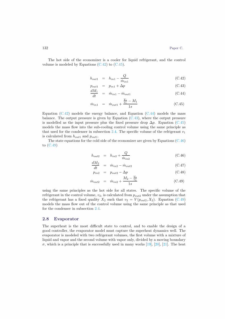
132 Paper C.
The hot side of the economizer is a cooler for liquid refrigerant, and the controlvolume is modeled by Equations (C.42) to (C.45).
hout1 = hin1 −Q
min1(C.42)
pout1 = pin1 + ∆p (C.43)
dM1
dt= min1 − mout1 (C.44)
min1 = mout1 +V1
v1− M1
1s(C.45)
Equation (C.42) models the energy balance, and Equation (C.44) models the massbalance. The output pressure is given by Equation (C.43), where the output pressureis modelled as the input pressure plus the fixed pressure drop ∆p. Equation (C.45)models the mass flow into the sub-cooling control volume using the same principle asthat used for the condenser in subsection 2.4. The specific volume of the refrigerant v1
is calculated from hout1 and pout1.The state equations for the cold side of the economizer are given by Equations (C.46)
to (C.49)
hout2 = hin2 +Q
min2(C.46)
dM2
dt= min2 − mout2 (C.47)
pin2 = pout2 − ∆p (C.48)
mout2 = min2 +M2 − V2
v2
1s(C.49)
using the same principles as the hot side for all states. The specific volume of therefrigerant in the control volume, v2, is calculated from pout2 under the assumption thatthe refrigerant has a fixed quality X2 such that v2 = V (pout2, X2). Equation (C.49)models the mass flow out of the control volume using the same principle as that usedfor the condenser in subsection 2.4.
2.8 Evaporator
The superheat is the most difficult state to control, and to enable the design of agood controller, the evaporator model must capture the superheat dynamics well. Theevaporator is modeled with two refrigerant volumes, the first volume with a mixture ofliquid and vapor and the second volume with vapor only, divided by a moving boundaryσ, which is a principle that is successfully used in many works [19], [20], [21]. The heat
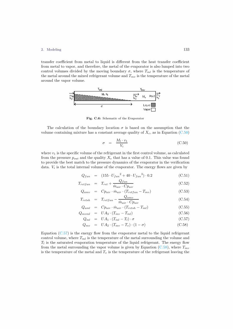
2. Modeling 133
transfer coefficient from metal to liquid is different from the heat transfer coefficientfrom metal to vapor, and therefore, the metal of the evaporator is also lumped into twocontrol volumes divided by the moving boundary σ, where Tml is the temperature ofthe metal around the mixed refrigerant volume and Tmv is the temperature of the metalaround the vapor volume.
Fig. C.6: Schematic of the Evaporator
The calculation of the boundary location σ is based on the assumption that thevolume containing mixture has a constant average quality of Xe, as in Equation (C.50)
σ =Ml · v1
Vi
(C.50)
where v1 is the specific volume of the refrigerant in the first control volume, as calculatedfrom the pressure pout and the quality Xe that has a value of 0.1. This value was foundto provide the best match to the pressure dynamics of the evaporator in the verificationdata. Vi is the total internal volume of the evaporator. The energy flows are given by
Qfan = (155 · Ufan2 + 40 · Ufan
3) · 0.2 (C.51)
Tretfan = Tret +Qfan
mair · Cpair
(C.52)
Qamv = Cpair · mair · (Tretfan − Tmv) (C.53)
Tretsh = Tretfan −Qamv
mair · Cpair
(C.54)
Qaml = Cpair · mair · (Tretsh − Tml) (C.55)
Qmvml = UA3 · (Tmv − Tml) (C.56)
Qml = UA1 · (Tml − Tl) · σ (C.57)
Qmv = UA2 · (Tmv − Tv) · (1 − σ) (C.58)
Equation (C.57) is the energy flow from the evaporator metal to the liquid refrigerantcontrol volume, where Tml is the temperature of the metal surrounding the volume andTl is the saturated evaporation temperature of the liquid refrigerant. The energy flowfrom the metal surrounding the vapor volume is given by Equation (C.58), where Tmv
is the temperature of the metal and Tv is the temperature of the refrigerant leaving the

134 Paper C.
evaporator calculated from the output pressure and enthalpy. The heat transfer coeffi-cients UA1 and UA2 were found to be 3510 J/K and 1930 J/K, respectively, through thesteady-state experiment described in Section 2.4. The value of UA3 was set to 50 J/K.Because the salient dynamics of the refrigeration system are closely related to the metaldynamics [8], it is assumed that the air that passes through the evaporator is cooled tothe metal temperature, and therefore, the energy flows from air to metal given in Equa-tions (C.53) and (C.55) yield the energy that is required to reach the metal temperature.The evaporator is a counter-flow heat exchanger, and therefore, the air passes over thesuper heating section of the evaporator before the evaporation section. Therefore, tocalculate the energy flow for each of the sections, the air temperatures at the input andoutput of the sections must be available. When the air enters the refrigeration unit, itpasses over the fans before it enters the evaporator, and therefore, the input air tem-perature on the evaporator is slightly higher than Tret due to the energy added by thefan given in Equation (C.51). The fan motor has a heat loss of 20%, and its speed isgiven by Ufan, which is an integer between 0 and 2, corresponding to off, low speed andhigh speed, respectively. Equation (C.52) calculates the air temperature after the fanTretfan as the return temperature from the container, Tret, plus the heat added by thefan. In Equation (C.53), the energy required to decrease the airflow temperature fromTretfan to Tmv, the temperature of the metal around the vapor volume, is calculated.Qamv is then used to calculate the temperature drop of the air over the super heatingpart of the evaporator in Equation (C.54), and the resulting air temperature, Tretsh,is then used to calculate Qaml, which is the energy required to decrease the airflowtemperature from Tretsh to the metal temperature around the liquid volume, Tml. Themetals around the two control volumes are divided by the artificial moving boundaryσ but are still physically connected, and therefore, there is also an energy flow betweenthe two volumes, which is modeled by Equation (C.56).
The energy flow from refrigerant to the metal is modeled by simple heat transfersin Equations (C.57) and (C.58), where the energy flow is the product of a heat transferconstant and the temperature difference between metal and refrigerant in the controlvolume. The sizes of UA1, UA2 and UA3 were determined by simulation experimentson the evaporator model over a range of working points that spans the normal area ofoperation for the refrigeration system.
The airflow over the evaporator is driven by a fan that has rotational inertia, andthe air has some inertia itself; therefore, the airflow does not instantly change when thefan speed is changed. This behavior is modeled by Equations (C.59) and (C.60):
¯mair =Ufan
2 · 3400.5 + Ufan3 · −1103.5
3600 · ρair
(C.59)
∆mair
∆t=
¯mair − mair
10s(C.60)
In Equation (C.59), the instant mass flow of the air, ¯mair, is calculated by a polynomial

2. Modeling 135
fit that yields the correct mass flow at the discrete speeds of the fan. The instant massflow is then used in Equation (C.60) as a reference for the actual airflow, mair, in afirst-order difference with a time constant of 10 seconds.
The remaining state equations are given by Equations (C.61) to (C.68)
dTml
dt=
Qaml − Qml + Qmvml
Mm · Cpm · σ(C.61)
dTmv
dt=
Qamv − Qmv − Qmvml
Mm · Cpm · (1 − σ)(C.62)
pout = P HV
(
hv,Vi − Vl
Mv
)
(C.63)
hl = hin +Qml
min
(C.64)
hv = hlv +Qmv
mlv
(C.65)
dMl
dt= min − mlv (C.66)
dMv
dt= mlv − mout (C.67)
Tsup = Tretfan +Qaml + Qamv
Cpair · mair
(C.68)
Equations (C.61) and (C.62) model the change in metal temperature as the net flow ofenergy into the control volume divided by the specific heat Cpm and mass Mm of themetal. The amount of metal in each of the control volumes depends on σ, and therefore,the mass is divided by the boundary.
The pressure in the evaporator, pout, is calculated by table lookup and given byEquation (C.63). It is assumed that the pressure is the same in both control volumesand calculated from the state of the refrigerant in the vapor volume using the specificenthalpy and the density of the vapor. The density is calculated from the mass ofthe vapor and the volume of the vapor, which is the total volume of the evaporatorminus the volume of the liquid refrigerant. Mv and vv are the mass and specific volumefor the vapor volume, respectively, and Vl is the volume occupied by the liquid in theevaporator. The energy balances for the liquid and vapor control volumes are given byEquations (C.64) and (C.65), respectively. The enthalpy of the refrigerant moving fromthe liquid to the vapor volume, hlv, is the dew point enthalpy at the pressure in theevaporator, pout. The mass flow between the two volumes is given by
mlv =Qml
hdew − hin
(C.69)
which is the amount of refrigerant that can be evaporated by Qml. The mass balancesfor the two control volumes are given in Equations (C.66) and (C.67) as the net sum

136 Paper C.
of the mass flows in and out of the respective volumes. The final state equation ofthe evaporator is for the supply air to the cargo hold of the container, Tsup, whichis modeled as the instantaneous temperature drop from the temperature after the fanTretfan calculated from the cooling energy flows Qaml and Qamv, the air mass flow mair
and the specific heat of air Cpair. The air flow over the evaporator is high comparedto the mass of the air around the evaporator, and therefore, the dynamics of the airaround the evaporator is neglected.
2.9 Box
The box is the main thermodynamic capacitance in the container due to the large massesof the aluminum T-floor and the cargo. The cargo and the T-floor have a large surfacearea; therefore, the temperature of the air inside the container has a strong couplingto the temperature of these two control volumes. The model of the box consists of thethree main thermal capacities: the temperatures of the cargo, the T-floor and the air;their state equations are shown in Equations (C.70) to (C.72).
dTair
dt=
Qca + Qaa + Qfa + Qfan − Qcool
Mair · Cpair
(C.70)
dTfloor
dt=
Qaf − Qfa
Mfloor · Cpfloor
(C.71)
dTcargo
dt=
−Qca
Mcargo · Cpcargo
(C.72)
The change in air temperature is modeled by Equation (C.70), where Qca is the energyflow from the cargo to the air, Qaa is the energy flow through the walls from the outsideto air, Qfa is the energy flow from the floor to the air, Qfan is the energy from inertiaadded to the air by the fan that is converted to heat as the air slows down, and Qcool
is the cooling provided by the evaporator. Qcool is calculated from the mass flow ofthe air, the specific heat of air and the temperature difference between the return andsupply temperature:
Qcool = Cpair · mair · (Tret − Tsup) (C.73)
Qaa = (Tamb − Tair) · UAamb · 0.81 (C.74)
Qaf = (Tamb − Tfloor) · UAamb · 0.19 (C.75)
Qca = (Tcargo − Tair) · UAcargo (C.76)
Qfa = (Tfloor − Tair) · UAfloor (C.77)
Qfan = (155 · Ufan2 + 40 · Ufan
3) · 0.8 (C.78)
The energy flows between control volumes are all modeled as standard heat transferswith a temperature difference multiplied by a heat transfer coefficient UA∗. The heat

3. Results 137
transfer coefficients UAcargo and UAfloor were determined through experiments on acontainer with cargo in which the cooling capacity was increased, and the heat transfercoefficients were calculated from the dynamical response of the floor and cargo tem-peratures to the change in air temperature. The determined values were 500 J/K forUAcargo and 1100 J/K for UAfloor. The heat transfer coefficient for the walls and floorof the container is UAamb and specified by the manufacturer to be 43 J/K. The area ofthe floor corresponds to 0.19 times the total surface area of the container, and therefore,Equations (C.75) and (C.74) are multiplied by 0.19 and 0.81, respectively.
3 Results
The performance of the model is evaluated by running the model in open-loop withcontrol inputs sampled from a real container running with closed-loop control. Mea-surements from the container are then compared with the corresponding states from themodel, and the error distribution for each of the measured variables is presented. Thetest sequence inputs were obtained from a container loaded with pork that was steppedthrough different cooling capacities at a set point of -20◦C. The sampled variables thatare used as model inputs are all the control inputs plus the ambient temperature. Theinitial conditions of the model was set to reflect the initial conditions of the sampleddata from the real container. The simulation period is three hours, during which thecontainer is running in both start/stop and continuous modes at different cooling pow-ers. The fact that the model is able to run in open loop for such a long period withoutdiverging outside the stable operational envelope of the model is due to the slow dy-namics and a certain degree of self-stabilization that exists in the refrigeration system.The error distributions for the measured variables are shown in the histogram in FigureC.7, the results from the three-hour test run can be seen in Figure C.8, and a closeupof the first 30 minutes can be seen in Figure C.9.
In the first subplot of Figures C.8 and C.9, the control signals applied to the modelare shown. Fcpr is the compressor speed, Vexp is the evaporator expansion valve open-ing, Veco is the economizer expansion valve opening, Fcond is the condenser fan speed,and Fevap is the evaporator fan speed.
The measurements that are available for verification of the model cannot be used todirectly verify that certain component models, such as the compressor and expansionvalves, have the correct mass flow. There is no significant drift on the suction pressure,which indicates that the mass flow of the evaporator expansion valve and the first stageof the compressor are the same, but it does not provide any indication that the massflow is correct. To obtain indication that the mass flow is correct, the cooling capacitiesof the real unit and the model were calculated from the supply and return temperaturesand the airflow. If the two cooling capacities match and the energy balance of the modelholds, then the mass flow of the compressor and the expansion valve models matchesthe real system. The cooling capacity of the model is accurate when the unit is running

138 Paper C.
−3 −2 −1 0 1 2 30
10
20
30Temperature Error Distribution
Error [K]
Fre
quen
cy [%
]
TcTsupTretTsucT0
−400 −300 −200 −100 0 100 200 300 4000
5
10Cooling Capacity Error Distribution
Error [W]
Fre
quen
cy [%
]
Fig. C.7: Model error distribution
continuously, but it is too large in the initial start/stop phase of the test, which couldbe due to a compressor model that removes too much refrigerant from the evaporator atlow speed or due to too much sub-cooling on the refrigerant from the economizer model.When the compressor is running continuously, the cooling capacity shows a very goodmatch to the model data throughout the simulation, indicating that the componentmodels are able to accurately reflect the static behavior of the real system.
The saturated discharge temperature of the condenser matches the overall trends,but the dynamics are inaccurate due to the simple single control volume model thatwas used. From the start/stop phases of the test, it can be observed that the pressureincreases rapidly just after the start of the compressor and the slowly drops again. Thisbehavior is caused by the inertia of the liquid in the condenser, which is not modeled,and therefore, this dynamic behavior is missing from the model. The dynamic responsefrom changes in Tamb to changes in Tc is too weak, and this could be due to the lumpedmodel. Due to the proximity of the condenser air intake and discharge, some amountof recirculation that is highly sensitive to the air flow around the container occurs. Thecontainer was located in a yard with other running containers when the data used forverification of the model were recorded, and this could have also caused disturbances in

3. Results 139
0
20
40
FcprVexpVecoFcondFevap
0
1000
2000
3000
Coo
ling
Cap
[W]
QCool measQCool model
10
15
20
Tc
[°C
]
Tc measTc modelTamb
0 20 40 60 80 100 120 140 160 180−24
−22
−20
Tsu
p, T
ret [
°C]
Tsup measTsup modelTret measTret model
0 20 40 60 80 100 120 140 160 180
−24
−22
−20
Time [min]
Tsu
c, T
0 [°
C]
Tsuc measTsuc modelT0 measT0 model
Fig. C.8: Model verification results
the airflow around the refrigeration unit end of the container that impacts the recircu-lation of the condenser air.
The return temperature has very slow dynamics due to the large thermal inertiaof the cargo, but the model is within ±0.25K of the measured return temperature.Because the cargo heat transfer coefficient and thermal inertia change depending onwhat is shipped in the container, it is only important to have an accurate model of the
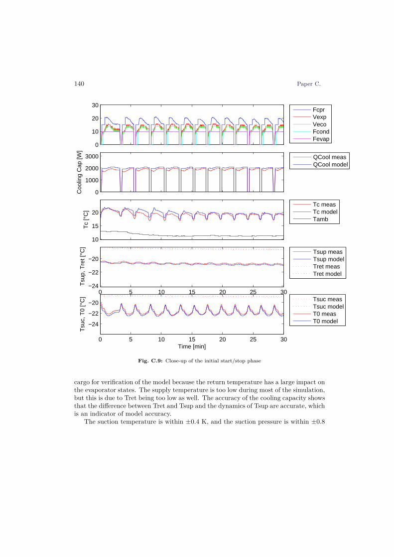
140 Paper C.
0
10
20
30
FcprVexpVecoFcondFevap
0
1000
2000
3000
Coo
ling
Cap
[W]
QCool measQCool model
10
15
20
Tc
[°C
]
Tc measTc modelTamb
0 5 10 15 20 25 30−24
−22
−20
Tsu
p, T
ret [
°C]
Tsup measTsup modelTret measTret model
0 5 10 15 20 25 30
−24
−22
−20
Time [min]
Tsu
c, T
0 [°
C]
Tsuc measTsuc modelT0 measT0 model
Fig. C.9: Close-up of the initial start/stop phase
cargo for verification of the model because the return temperature has a large impact onthe evaporator states. The supply temperature is too low during most of the simulation,but this is due to Tret being too low as well. The accuracy of the cooling capacity showsthat the difference between Tret and Tsup and the dynamics of Tsup are accurate, whichis an indicator of model accuracy.
The suction temperature is within ±0.4 K, and the suction pressure is within ±0.8

3. Results 141
K, which shows that the model of the evaporator is a good match to the real systemboth statically and dynamically and that there is some accumulation of errors over time.This is however in open loop where small inaccuracies can accumulate over time, andwhen the loop is closed in controller experiments, this buildup disappears because thecontroller compensates for model inaccuracy. In the beginning of the test, there is amismatch because the initial conditions of the model were not perfectly established,but the model quickly stabilized. A close-up of the beginning of the test is shown inFigure C.9, where the match is good because errors have not yet accumulated. Theperformance of the model on the temperatures on the evaporator is very accurate in thefirst 110 minutes, but later in the test, sequence errors begin to accumulate, resultingin an inaccurate suction pressure two hours into the test sequence.
From the temperature error distribution shown in Figure C.7, it can be observed thatall temperatures except the saturated condenser pressure are within ±0.8 K, demon-strating that the model matches the real system well on these parameters. The modelis intended to be used to test controllers that are being developed for the container,as a simulation tool and as the basis for generating linear models that can be used todevelop controllers. These controllers must be robust to sensor inaccuracies that can bean order of magnitude larger than the model inaccuracy, and therefore, it is concludedthat the model accuracy is adequate for the measurements on the evaporator and thecargo hold. To design a good controller for the condenser, a better model with more ac-curate dynamics and a better response to changes in ambient temperature is required,but because the salient dynamics are present in the current model, it would also bepossible to use it for controller design.

142 References
4 Conclusion and Future Work
4.1 Conclusion
In this study, a dynamical simulation model of a refrigeration container and its refriger-ation unit has been developed, with the objective of being sufficiently accurate for use incontroller design and simulation experiments. The results demonstrated that adequateperformance can be reached with a model in which small terms and fast dynamics areneglected and assumptions are used rather than first principles, which corresponds toa reduction in the model order. The results verify that the dynamics of a containerrefrigeration system can be modeled by the thermal masses in the heat exchangers, themetal in the cargo hold and the cargo, with a model of the refrigeration cycle thatincludes normal mass balances but with steady-state momentum and energy balances.The model exhibits good matching of both static and dynamical behaviors, and there-fore, the model can be used for controller development where little or no tuning isnecessary when moving from the model to the real system.
4.2 Future Work
Because the model is to be used in the development of controllers for use on a realsystem, the model also has to reflect the important aspects of this system. One aspectthat has been ignored in this work is ice buildup on the evaporator. Ice degrades theairflow over the evaporator and the heat transfer coefficient from the evaporator metalto the air and has an impact on efficiency that cannot be neglected. The dynamicalresponse of the discharge pressure to the ambient temperature must be improved to beable to develop a controller that has proper disturbance rejection of sudden changesin the ambient temperature. Another useful improvement would be better robustnessof the equations on which the model is based, particularly with respect to the model’sability to handle both liquid and vapor refrigerants in all control volumes.
5 Acknowledgment
The authors gratefully acknowledge the assistance from Kim Madsen from MCI forcounseling on modeling of the refrigeration container components and MCI for providinga container with cargo for testing.
References
[1] K. Sørensen and J. Stoustrup, “Modular modelling and simulation approach - ap-plied to refrigeration systems,” in Proceedings of IEEE International Conference on
References 143
Control Applications, San Antonio, Texas, USA, September 2008, pp. 983 – 988.doi:10.1109/CCA.2008.4629691
[2] K. Sørensen, D. Jens, and J. Stoustrup, “Modular simulation of reefer con-tainer dynamics,” Published online before print in Simulation, December 2013.doi:10.1177/0037549713515542
[3] J. Cai, J. Stoustrup, and J. Jorgensen, “Preventing refrigerated foodstuffsin supermarkets from being discarded on hot days by mpc,” in Pro-ceedings of the 17th IFAC World Congress, Seoul, Korea, 2008. [Online].Available: http://www.control.aau.dk/~jakob/selPubl/papers2008/ifacwc_2008_3.pdf. doi:10.3182/20080706-5-KR-1001.01880
[4] R. G. M. van der Sman and G. J. C. Verdijck, “Model predictions andcontrol of conditions in a ca-reefer container,” in ISHS Acta Horticulturae 600:VIII International Controlled Atmosphere Research Conference, AgrotechnologicalResearch Institute ATO, P.O. box 17, 6700 AA Wageningen, the Netherlands,2003, pp. 163–171. [Online]. Available: http://www.actahort.org/members/showpdf?booknrarnr=600_20
[5] G. J. C. Verdijck, H. A. Preisig, and G. van Straten, “Direct productquality control for energy efficient climate controlled transport of agro-material,”Journal of Process Control, vol. 15, no. 2, pp. 235 – 246, 2005. [Online].Available: http://www.sciencedirect.com/science/article/pii/S0959152404000514.doi:10.1016/j.jprocont.2004.04.004
[6] L. Filina and S. Filin., “An analysis of influence of lack of the electricity sup-ply to reefer containers serviced at sea ports on storing conditions of cargoescontained in them,” in Polish Maritime Research, vol. 15, 2009, pp. 96–102.doi:10.2478/v10012-008-0002-z
[7] L. S. Larsen, C. Thybo, and H. Rasmussen, “Intelligent control - optimizing theoperation of refrigeration systems under daily variations in ambient temperature,”in Danske Køledage, March 15th-16th, 2007. Proceedings of Danske Køledage 2007.,2007.
[8] B. Rasmussen, A. Musser, and A. Alleyne, “Model-driven system identification oftranscritical vapor compression systems,” IEEE Transactions on Control SystemsTechnology, vol. 13, no. 3, pp. 444–451, 2005. doi:10.1109/TCST.2004.839572
[9] Guo-liang Ding, “Recent developments in simulation techniques for vapour-compression refrigeration systems,” International Journal of Refrigeration, vol. 30,no. 7, pp. 1119–1133, 2007. doi:10.1016/j.ijrefrig.2007.02.001
144 References
[10] R. Zhou, T. Zhang, J. Catano, J. T. Wen, G. J. Michna, Y. Peles, and M. K.Jensen, “The steady-state modeling and optimization of a refrigeration system forhigh heat flux removal,” Applied Thermal Engineering, vol. 30, no. 16, pp. 2347 –2356, 2010. [Online]. Available: http://www.sciencedirect.com/science/article/pii/S135943111000219X. doi:10.1016/j.applthermaleng.2010.05.023
[11] L. F. Shampine and S. Thompson, “Stiff systems,” vol. 2, no. 3, p. 2855, 2007.
[12] M. Skovrup, “Windali - an open-structured component modeling and simulationprogram based on standard programming languages,” in Proceedings of SIMS Con-ference. Lyngby, 2000, pp. 157–172.
[13] M. J. Skovrup, “Refrigerant equations library,” Department of MechanicalEngineering, Section of Energy Engineering, Technical University of Denmark,Nils Koppels Allé, Building 402 DK-2800 Lyngby, DENMARK. [Online]. Available:http://www.et.web.mek.dtu.dk/WinDali/Files/RefEqns3.10.ZIP
[14] K. Prölss, G. Schmitz, D. Limperich, and M. Braun, “Influence of refrigerantcharge variation on the performance of an automotive refrigeration system,” inInternational Refrigeration and Air Conditioning Conference, Paper 843, 2006.[Online]. Available: http://docs.lib.purdue.edu/iracc/843
[15] T. Henzinger, “The theory of hybrid automata,” in Logic in Computer Science,1996. LICS ’96. Proceedings., Eleventh Annual IEEE Symposium on, 1996, pp.278–292. doi:10.1109/LICS.1996.561342
[16] R. Koury, L. Machado, and K. Ismail, “Numerical simulation of a variablespeed refrigeration system,” International Journal of Refrigeration, vol. 24, no. 2,pp. 192 – 200, 2001. [Online]. Available: http://www.sciencedirect.com/science/article/pii/S0140700700000141. doi:10.1016/S0140-7007(00)00014-1
[17] H. Li, J. E. Braun, and B. Shen, “Modeling adjustable throat-area expansionvalves.” International Refrigeration and Air Conditioning Conference, 2004, p.Paper 705. [Online]. Available: http://docs.lib.purdue.edu/iracc/705/
[18] Danfoss, “Brazed plate heat exchanger datasheet,” 2014. [Online].Available: http://www.ra.danfoss.com/TechnicalInfo/Literature/Manuals/24/DKQBPD000B102.pdf
[19] M. Willatzen, N. Pettit, and L. Ploug-Sørensen, “A general dynamic simulationmodel for evaporators and condensers in refrigeration. part i: moving-boundary formulation of two-phase flows with heat exchange,” InternationalJournal of Refrigeration, vol. 21, no. 5, pp. 398 – 403, 1998. [Online].Available: http://www.sciencedirect.com/science/article/pii/S0140700797000911.doi:10.1016/S0140-7007(97)00091-1
References 145
[20] N. Pettit, M. Willatzen, and L. Ploug-Sørensen, “A general dynamic simulationmodel for evaporators and condensers in refrigeration. part ii: simulation andcontrol of an evaporator,” International Journal of Refrigeration, vol. 21, no. 5,pp. 404 – 414, 1998. [Online]. Available: http://www.sciencedirect.com/science/article/pii/S0140700797000923. doi:10.1016/S0140-7007(97)00092-3
[21] H. Rasmussen, C. Thybo, and L. Larsen, Nonlinear Superheat and EvaporationTemperature Control of a Refrigeration Plant. Pergamon Press, 2006, pp. 252–254. doi:10.3182/20061002-4-BG-4905.00043

146 References

Paper D
Adaptive MPC for a Refrigerated Container
Kresten K. Sørensen and Jakob Stoustrup
Submitted to: Control Engineering Practice, November 2013.

Copyright c© 2013 Elsevier Science Ltd. All rights reserved.The layout has been revised.

149
Abstract
In this work, the potential energy savings from adapting to daily ambient temperaturedifferences for frozen cargo in reefer containers are studied using a model of the StarCool reefer. The objective is to create a controller that can be implemented on anembedded system, and a range of methods are used to reduce the computational load. Acombination of MPC and traditional control is used, and the accuracy of the MPC isenhanced with an on-line update of the model parameters. The simulation experimentsshow that potential energy savings of up to 21% are achieved when the MPC is allowedto control both the cooling capacity and the ventilation of the cargo area. The largestcost reduction is achieved through a reduced ventilation rate.
Nomenclature
Latin symbolsM Mass (kg)Q Energy flow (W)V Fan speedT Temperature (C◦)Cp Specific heat (J/(Kg K))C Heat capacity (J/K))α Heat transfer coefficient (W/K)P Power (W)
Subscripts
air Air in the cargo hold
amb Ambientfloor Floor of the cargo holdcool Cooling capacityfan Evaporator fancargo Cargo inside the cargo holdsup Supply air to cargo holdret Return air from cargo holdbox Walls of the cargo holds Slackc Compressormin Minimummax Maximum

150 Paper D.
1 Introduction
A large amount of perishable cargo is currently transported by sea in reefer containers.By mid-2008, the fleet consisted of 4500 reefer vessels with a combined reefer capac-ity of 11.4 million TEU1, and the capacity is predicted to increase by 69% by 2013;see [1]. These reefer containers are powered by electricity with a consumption of upto 6kW per TEU, depending on the ambient temperature and the temperature insidethe container itself. With an average consumption of 3.6 kW per TEU, this yields acombined consumption of 41 GW, which is, on average, 8.9 MW per ship; see [2] and[3]. Previously, this energy consumption was considered to be insignificant with respectto the large amount of energy used to propel the ship, but due to increasing oil prices,greater competition in the shipping market and the environmental impact of shipping,reducing the energy consumption of reefer containers has become of interest.
The control solutions currently employed are based on classical control theory, inwhich the individual components are controlled by separate controllers, with a limitedamount of controller interconnections and gain scheduling. The objective of these con-trollers is to maintain the temperature inside the container close to a setpoint at ambienttemperatures between -20C◦ and +37C◦ (hot side). The setpoint is in the range of -29C◦ to +25C◦ (cold side). Due to the large range of operation on the hot and coldsides and the non-linearities in the refrigeration system, the controllers used must beconservative to provide stability over the entire area of operation.
Fruits and vegetables are generally quite sensitive to atmosphere and temperaturevariations, which means that the cargo temperature and air composition in the containermust be kept within certain limits. This reduces the potential for control optimizationswith respect to energy consumption by using the thermal inertia of the cargo as a buffer.It has been shown that the cost of operating a refrigeration system may be decreasedby using thermal inertias in the system as a buffer to offset cooling to periods where thecost is low. In [4], the cost of a running household heat pump is lowered by using anMPC that is fed the forecasted cost of electricity. Exploiting ambient conditions to lowerthe energy consumption of building HVAC systems while respecting occupant comfortconstraints is demonstrated in [5, 6, 7, 8] and is shown to significantly reduce energyconsumption while ensuring good occupant comfort. A learning-based approach for thepre-cooling of foodstuffs to avoid saturation of the refrigeration system on hot daysis demonstrated by [9] using an MPC that is updated on-line with the learning-basedconstraints and predicted future load. In [10], an MPC is used to control the productquality of chilled cargo in refrigerated containers with the primary focus on modellingand controlling the cargo quality, resulting in a reduction of mass loss in the cargo dueto evaporation and lower energy consumption due to a reduced ventilation rate.
An existing energy saving control strategy that is in use is QUEST (see [11]), whichis a control scheme for fruits and vegetables that allows for larger supply air temperature
1Twenty Foot Equivalent. The equivalent of a twenty foot reefer container.

1. Introduction 151
variances and lower fan speeds based on a predefined set of rules. This can be allowedbecause research has shown that there is no degradation in produce quality if the supplyair temperature is varied around the setpoint due to the thermal insulation of theproduce packaging and the slow metabolic rates of the produce; see [12]. The rules forventilation rate and temperature variation have been determined by testing a wide rangeof different types of fruits and vegetables and ensuring that the cargo quality remainsunaffected by the variations. There are various rules for different product classes, andthey have been designed dependent of the temperature setpoint to make it easy tooperate. This is important because it is infeasible to educate loading crews all overthe world in complex set up procedures. For reefer containers without a VSD (variablespeed drive) on the compressor, the energy savings from using QUEST can be as high as53% because the refrigeration system is very inefficient at part load, and for containerswith a VSD on the compressor, the energy savings are smaller but still significant.
For frozen goods, the rules that must be followed to preserve cargo quality are morelenient than those for chilled goods, and therefore, the cargo thermal inertia can beused to offset cooling from the periods where the system is less efficient to periodswhere the system is more efficient. The ambient temperature has a direct influenceon the condensation pressure and thus also on the system efficiency, which leads tothe possibility of moving some cooling from the day where the ambient temperatureis high to the night where the ambient temperature is lower. Another approach forreducing energy consumption is to reduce the amount of ventilation inside the cargohold because the power consumed by the fans has a dual impact on the cost of runningthe system. The fans consume energy, which is added to the cost of running the system,but the kinetic energy that the air receives from the fans is eventually converted to heatinside the container, which means that it must be removed by the refrigeration system.Therefore, investigating the potential of optimizing how the fans are used is of interest.
Model predictive control (MPC) was introduced in the petro-chemical industry tocontrol difficult processes with long delays and unknown states, but today, MPC is usedin a wide range of applications, such as power plant control and the automotive industry.MPC is used for optimizing control of processes with respect to known future demandsor known future changes in external conditions while remaining within a given set ofconstraints. The performance of MPC is dependent on the quality of the model on whichit is based because it is used to predict the behaviour of the system over the predictionhorizon. For systems where the model dynamics may change, either a non-linear or anadaptive linear approach must be used to retain the performance and to avoid violatingthe imposed constraints.
A refrigeration system has several degrees of freedom, meaning that the same coolingcapacity can be obtained with different actuator setpoints. [13] showed that selectingthe correct setpoints can have a high impact on the efficiency of the refrigeration system,and therefore, any controller aiming to save energy should focus on selecting the correctsetpoints.

152 Paper D.
In this study, the potential for energy savings by adapting to daily ambient tempe-rature differences is studied for frozen cargo in refrigerated containers. The observationfrom [10] that adequate cooling may be achieved at a lower ventilation rate is used toformulate control laws for an MPC that ensures optimal utilization of the fans whenthey are running. Cargo parameters such as thermal inertia and heat transfer coefficientare estimated and used as the basis for the MPC model, resulting in flexibility towardschanges in these parameters that does not exist in QUEST. Furthermore, the MPCis set up to exploit daily variations in ambient temperature by cooling more when theambient temperature is low and when the efficiency of the refrigeration system is higher.This extra cooling is "stored" in the cargo thermal inertia, allowing for a smaller coolingeffort during the day when the ambient temperature is high and the refrigeration systemefficiency is low. The future ambient temperature is predicted from measurements fromthe last 24 hours by an oscillator and a simple phase-locked loop and fed to the MPC.
In this paper, we present an adaptive MPC controller that utilizes the same principlesas QUEST but with the added benefit of adapting to cargo parameters and daily cyclesin ambient temperature for increased energy efficiency. The potential energy savings atdifferent ambient temperatures and fan control methods are investigated and presented.The computational load is reduced due to varying step sizes in the prediction horizonand linearizing local controllers, which enables the use of a reduced linear model for theMPC.
In the following, the methods used in this paper are described, starting with a shortintroduction to the refrigeration system in Section 2.1. Then, a description of theparameter and state estimators used by the controller follows in Section 2.2. Finally,the controller itself is described in Section 2.3.
2 Methods
2.1 Refrigeration System Simulation Model
The refrigeration container used in this paper is constructed by Maersk Container In-dustry and is equipped with a Star Cool refrigeration unit; see [14]. A refrigerationcontainer is an insulated box with a door for loading cargo at one end and a refrigera-tion system at the other end, as shown in Figure D.1.
The cargo is kept cold by air that is circulated from the evaporator towards thedoor end of the container through a T-profile floor, which allows air to enter small gapsbetween the produce. The air is heated by the produce or the walls and rises to theceiling of the box, where the hot air flows back to the evaporator. Natural convectionis not sufficient to ensure an even distribution of air in the box, and therefore, the airflow is driven by fans located above the evaporator. The energy from these fans endsup as heat in the box and has to be removed by the refrigeration system. Therefore, itis desirable to run the fans as little as possible. It is however necessary to start the fans

2. Methods 153
Fig. D.1: Airflow in the Refrigeration Container
at regular intervals to be able to measure the air temperature in the box itself becauseno air temperature sensors are placed here and to prevent local hot-pockets of air fromforming and spoiling the produce.
Fig. D.2: Refrigeration System Schematic
A schematic of the refrigeration system used in this study is shown in Figure D.2.This refrigeration system is a two-stage cycle that uses an economizer to increase theefficiency of the system under high temperature differences between the cold and hotsides.
The compressor has high- and low-pressure stages, which are shown as two single-stage compressors in the figure. The compressor is equipped with a VSD, and the fansmay be either stopped, at half speed or at full speed. The expansion valves are pulsemodulated, that is, they can be either closed or fully open. These expansion valves arecontrolled by a PWM signal with a period of six seconds.

154 Paper D.
0
20
40
FcprVexpVecoFcondFevap
0
1000
2000
3000
Coo
ling
Cap
[W]
QCool measQCool model
10
15
20
Tc
[°C
]
Tc measTc modelTamb
0 20 40 60 80 100 120 140 160 180−24
−22
−20
Tsu
p, T
ret [
°C]
Tsup measTsup modelTret measTret model
0 20 40 60 80 100 120 140 160 180
−24
−22
−20
Time [min]
Tsu
c, T
0 [°
C]
Tsuc measTsuc modelT0 measT0 model
Fig. D.3: Simulation model verification results
−3 −2 −1 0 1 2 30
10
20
30Temperature Error Distribution
Error [K]
Fre
quen
cy [%
]
TcTsupTretTsucT0
−400 −300 −200 −100 0 100 200 300 4000
5
10Cooling Capacity Error Distribution
Error [W]
Fre
quen
cy [%
]
Fig. D.4: Simulation model error distribution
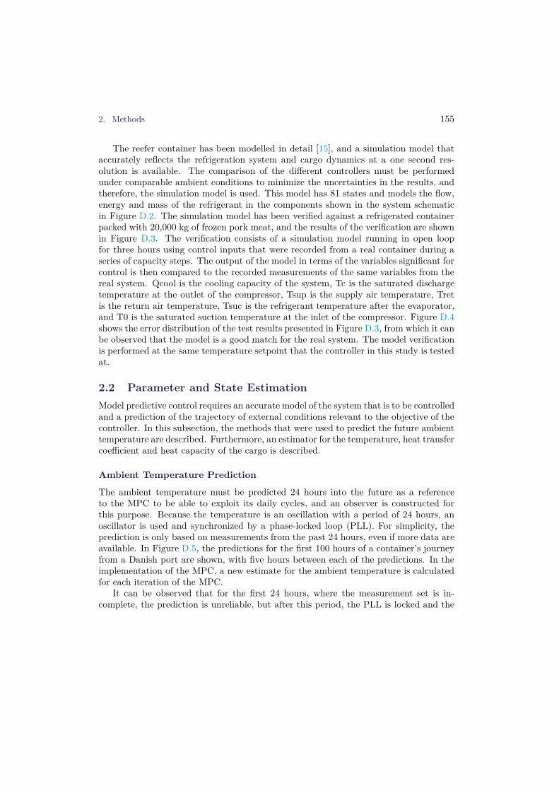
2. Methods 155
The reefer container has been modelled in detail [15], and a simulation model thataccurately reflects the refrigeration system and cargo dynamics at a one second res-olution is available. The comparison of the different controllers must be performedunder comparable ambient conditions to minimize the uncertainties in the results, andtherefore, the simulation model is used. This model has 81 states and models the flow,energy and mass of the refrigerant in the components shown in the system schematicin Figure D.2. The simulation model has been verified against a refrigerated containerpacked with 20,000 kg of frozen pork meat, and the results of the verification are shownin Figure D.3. The verification consists of a simulation model running in open loopfor three hours using control inputs that were recorded from a real container during aseries of capacity steps. The output of the model in terms of the variables significant forcontrol is then compared to the recorded measurements of the same variables from thereal system. Qcool is the cooling capacity of the system, Tc is the saturated dischargetemperature at the outlet of the compressor, Tsup is the supply air temperature, Tretis the return air temperature, Tsuc is the refrigerant temperature after the evaporator,and T0 is the saturated suction temperature at the inlet of the compressor. Figure D.4shows the error distribution of the test results presented in Figure D.3, from which it canbe observed that the model is a good match for the real system. The model verificationis performed at the same temperature setpoint that the controller in this study is testedat.
2.2 Parameter and State Estimation
Model predictive control requires an accurate model of the system that is to be controlledand a prediction of the trajectory of external conditions relevant to the objective of thecontroller. In this subsection, the methods that were used to predict the future ambienttemperature are described. Furthermore, an estimator for the temperature, heat transfercoefficient and heat capacity of the cargo is described.
Ambient Temperature Prediction
The ambient temperature must be predicted 24 hours into the future as a referenceto the MPC to be able to exploit its daily cycles, and an observer is constructed forthis purpose. Because the temperature is an oscillation with a period of 24 hours, anoscillator is used and synchronized by a phase-locked loop (PLL). For simplicity, theprediction is only based on measurements from the past 24 hours, even if more data areavailable. In Figure D.5, the predictions for the first 100 hours of a container’s journeyfrom a Danish port are shown, with five hours between each of the predictions. In theimplementation of the MPC, a new estimate for the ambient temperature is calculatedfor each iteration of the MPC.
It can be observed that for the first 24 hours, where the measurement set is in-complete, the prediction is unreliable, but after this period, the PLL is locked and the

156 Paper D.
0 20 40 60 80 100 1205
10
15
20
25
30
Time [h]
Tem
p [C
°]
Tamb EstimatesMeasured Tamb
Fig. D.5: Prediction of future ambient temperature
prediction improves. Due to a non-sinusoidal oscillation of the measured ambient tem-perature, the amplitude estimate can be off, but as shown later, the most importantfactor is that the phase is correct, and therefore, this predictor is adequate for the MPC.
Cargo State and Parameter Estimation
The quality of the solution to the optimization problem in the MPC is dependent on theaccuracy of the linear model used. Although the properties of the refrigeration systemare well defined, the properties of the cargo are very uncertain because reefer containersare used to transport a wide range of different goods. The largest thermal mass isgenerally the cargo, and therefore, it is also the most interesting property with respectto exploiting the daily variances in ambient temperature. If the cargo heat capacityis not known, the lowest value must be used to ensure that the constraints are notviolated because the lowest heat capacity also provides the fastest dynamics. Using thelowest possible heat capacity will limit the degree to which the variations in COP canbe exploited. To resolve this issue, a combined parameter estimator and unknown inputobserver is introduced, and the estimates are then used to update the MPC on-line.The observer is based on the model of the cargo hold and cargo of the reefer containers,which is presented in the simulation model described in Section 2.1. It has been modifiedto simulate the unknown states and estimate and update the parameters for the cargowhen conditions allow. Knowledge of parameter and state constraints are incorporated
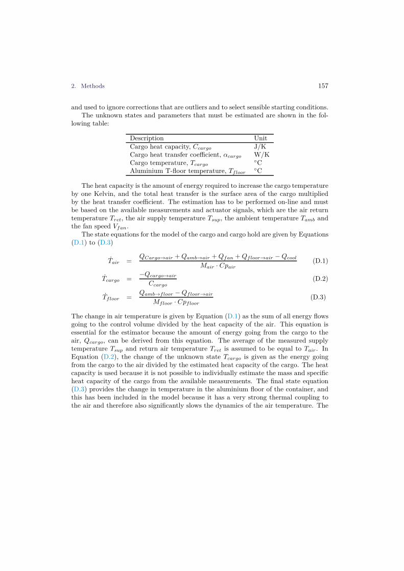
2. Methods 157
and used to ignore corrections that are outliers and to select sensible starting conditions.The unknown states and parameters that must be estimated are shown in the fol-
lowing table:
Description UnitCargo heat capacity, Ccargo J/KCargo heat transfer coefficient, αcargo W/KCargo temperature, Tcargo
◦CAluminium T-floor temperature, Tfloor
◦C
The heat capacity is the amount of energy required to increase the cargo temperatureby one Kelvin, and the total heat transfer is the surface area of the cargo multipliedby the heat transfer coefficient. The estimation has to be performed on-line and mustbe based on the available measurements and actuator signals, which are the air returntemperature Tret, the air supply temperature Tsup, the ambient temperature Tamb andthe fan speed Vfan.
The state equations for the model of the cargo and cargo hold are given by Equations(D.1) to (D.3)
Tair =QCargo→air + Qamb→air + Qfan + Qfloor→air − Qcool
Mair · Cpair
(D.1)
Tcargo =−Qcargo→air
Ccargo
(D.2)
Tfloor =Qamb→floor − Qfloor→air
Mfloor · Cpfloor
(D.3)
The change in air temperature is given by Equation (D.1) as the sum of all energy flowsgoing to the control volume divided by the heat capacity of the air. This equation isessential for the estimator because the amount of energy going from the cargo to theair, Qcargo, can be derived from this equation. The average of the measured supplytemperature Tsup and return air temperature Tret is assumed to be equal to Tair. InEquation (D.2), the change of the unknown state Tcargo is given as the energy goingfrom the cargo to the air divided by the estimated heat capacity of the cargo. The heatcapacity is used because it is not possible to individually estimate the mass and specificheat capacity of the cargo from the available measurements. The final state equation(D.3) provides the change in temperature in the aluminium floor of the container, andthis has been included in the model because it has a very strong thermal coupling tothe air and therefore also significantly slows the dynamics of the air temperature. The

158 Paper D.
heat transfers in the above equations are given by Equations (D.4) to (D.7):
Qamb→air = (Tamb − Tair) · (1 − β) · αbox (D.4)
Qamb→floor = (Tamb − Tfloor) · β · αbox (D.5)
Qfloor→air = (Tfloor − Tair) · αfloor (D.6)
BQcargo→air = (Tcargo − Tair) · αcargo (D.7)
Qcool = f (Tsup, Tret, Vfan) (D.8)
Qamb→air is the heat transfer from the surroundings to the air in the container throughthe walls, roof and ends of the cargo hold given by the temperature difference multipliedby the fraction of total surface area represented by the walls, roof and ends and the heattransfer coefficient αbox, which is 43 W
K[16]. The floor of the container also receives
some heat from the outside, as given by Equation (D.5) as the temperature differencemultiplied by the heat transfer coefficient αbox and the fraction of total surface arearepresented by the floor β, which is 0.190. The heat transfer from the floor to the air isgiven by Equation (D.6), where the heat transfer coefficient αfloor has been estimatedto be 5000 W
Kin a step response experiment. The energy going from the cargo to the
air, Qcargo→air, is given by Equation (D.7), and it includes two unknowns: the cargotemperature Tcargo and the heat transfer coefficient from the cargo to the air αcargo.Tair is the mean of the supply and return temperature for the air entering and leavingthe cargo hold, which is measured and thus very reliable. The cooling capacity deliveredby the refrigeration system is given by Equation (D.8), which is the calculated coolingcapacity from the temperature difference between the return and supply air and the airflow calculated from the fan speed Vfan.
There is an uncertainty in the heat influx through the container wall that dependson the air flow over the outside surface, rain and direct exposure to the sun. FromEquation (D.1), it can be observed that this will lead to an uncertainty in the estimationof Qcargo→air because Qfan, Qfloor→air and Qcool are known or can be measured.
The easiest state to estimate is the floor temperature because it will reach steadystate equilibrium between the ambient and air temperatures, which are both measured;therefore, if the floor temperature is estimated using Equations (D.5), (D.6) and (D.3),the estimated floor temperature will over time track the actual floor temperature.
The cargo temperature may be estimated using the same method as for the floorbecause it converges towards the air temperature, but this estimate includes the uncer-tainty of the parameters αcargo and Ccargo. If Equation (D.7) is inserted into Equation(D.2) and rearranged
Tcargo = (Tair − Tcargo) ·αcargo
Ccargo
(D.9)
it is clear that the change in cargo temperature is a first-order filter on the temperaturedifference between the air and the cargo, with a time constant that is given by the

2. Methods 159
two unknown parameters. Therefore, the cargo temperature estimate will convergetowards the mean air temperature, but it will only be accurate if the estimates ofαcargo and Ccargo are also accurate. It is assumed that the cargo is lumped and hasa uniform temperature, which is a simplification, but the model is able to reflect thesalient dynamics of the cargo on the time scale required by the controller.
A controller that uses the thermal inertia of the cargo to offset cooling to moreefficient conditions will cool the cargo in pulses, which in this case have a duration ofseveral hours, where the cargo temperature is decreased towards the lower temperatureconstraint. This excitation of the cargo dynamics is exploited to estimate the twounknown cargo parameters αcargo and Ccargo.
It is assumed that the system is linear and time invariant (LTI), and therefore, itcan be assumed that the heat transfer constant and the heat capacity of the cargo areconstant over time. This can be used to estimate αcargo by combining Equation (D.7)and Equation (D.10) and setting up two equations with two unknowns, which are solvedfor αcargo.
Qcargo→air−calc = Qcool − Qamb→air − Qfloor→air − Qfan (D.10)
Qcargo→air−calc−t1 = (Tcargo−t1 − Tair−t1) · αcargo (D.11)
Qcargo→air−calc−t2 = (Tcargo−t1 + Tcargo−delta − Tair−t2) · αcargo (D.12)
αcargo =Qcargo→air−calc−t2 − Qcargo→air−calc−t1
Tair−t1 − Tair−t2 + Tcargo−delta
(D.13)
The measurements of Qcargo→air−calc, Tcargo and Tair in Equations (D.11) and(D.12) must be taken at two different times that have a significant difference in Qcargo→air−calc
to produce a reliable estimate of αcargo. Tcargo−delta is the estimated change in cargotemperature between the two sample points, and because the cargo dynamics are sig-nificantly slower than the dynamics of the air, this change can be obtained from theestimated cargo temperature given by Equation (D.2). To prevent inaccurate estimatesdue to disturbances from the controller, it is required that the slope of Tsup is smallerthan 0.01K/s before the first set of measurements are acquired because this means thatthe cooling capacity is stable. This also ensures that fast higher-order dynamics havesettled and do not interfere with the accuracy of the estimate. The first measurement istaken at time = t1, and after 15 minutes, the second set of measurements are acquired,at time = t2. If the energy flows to the cargo, given by Equations (D.11) and (D.12),differs by more than 100 W, an update of αcargo is performed.
The heat capacity of the cargo is more difficult to estimate because the estimate hasto be inferred from the rate of change in air temperature measurements and the rateof change in the calculated energy flow from the cargo to the air. At a temperaturesetpoint of -20◦C, the refrigeration system is able to cool the cargo with up to 4 kW,which over a period of one hour is sufficient to cool the cargo used in this study by 0.686

160 Paper D.
K. This means that the slopes involved are very small and that the result is sensitiveto noise and disturbances. For αcargo, this may be resolved by determining the slopesover a period, thereby reducing the impact from noise and disturbances.
The slope of the difference between the cargo temperature and the mean air tempe-rature is given by Equation (D.14), where Qcargo→air−calc is the derivative of the energygoing from the cargo to the air.
Tcargo→air−diff =Qcargo→air−calc
αcargo
(D.14)
Tcargo = Tcargo→air−diff + Tair−mean (D.15)
Ccargo =Qcargo→air−calc
Tcargo
(D.16)
It is then possible to calculate the derivative of the cargo temperature as in Equation(D.15), where Tair−mean is the derivative of the measured mean air temperature inthe container. To acquire accurate derivatives, the acquisition period should be aslong as possible. The estimator requires 15 minutes where the cooling capacity of therefrigeration system is constant and large enough to ensure that at least 100 W of coolingis applied to the cargo before an update of the heat capacity of the cargo is calculated,as shown in Equation (D.16). In Figure D.6, the result of running the estimator on datafrom a real reefer container packed with 20,000 kg of bacon is shown.
On the top axes, the measured and estimated cargo temperature are shown. Theestimated heat capacity of the cargo has been converted to mass in metric tons, usingthe specific heat capacity for bacon, which is 1050 J
kg·K[17], and should therefore level
out at approximately 20. The data were obtained from a reefer that was located in anopen field and therefore subject to weather disturbances.
The controller was an early attempt at offsetting some cooling from day to nightusing MPC but without the estimator for the cargo parameters. The cooling thatis applied is mainly in pulses of 10 minutes, which is unfortunately a poor basis forestimating the cargo heat capacity because the pulses are too short to reliably estimatethe change in cargo temperature through the air temperature. Therefore, the estimateof the cargo heat capacity is updated only 15 times. The heat transfer coefficient forthis cargo has been estimated to be 550 W
Kfrom the measured cargo and air temperature
and the calculated power to the cargo.In Figure D.7, the result of the parameter estimation algorithm running on results
from the simulation model with an αcargo of 550 WK
and a 20,000 kg cargo mass with
a specific heat capacity of 1050 Jkg·K
is shown. Measurement noise has been added to
the simulation results. It is expected that αcargo converges towards 550 WK
and thatMcargo converges towards 20 t. The estimates quickly converge towards the true valuesimmediately after start up, and within 24 hours, the estimates are close to the correctvalues. In this test, the starting values have been set to demonstrate convergence,

2. Methods 161
−22
−21
−20
−19
−18T
emp
[°C
]
T
cargo
Tcargo−est
400
450
500
550
600
[W/K
]
α
cargo
0 50 100 150 200 250 30014
16
18
20
22
Time [h]
[t]
M
cargo
Fig. D.6: Cargo parameter estimator on reefer container measurements
but it is often possible to deduce the type of cargo from the temperature setpoint andsubsequently select better start values that will enable faster estimator convergence.
2.3 Controller Setup
A non-linear simulation model has been developed as described in Section 2.1, but thismodel has 81 states and a reduced model is desired because the controller eventually isto be used on an embedded hardware platform with limited resources. The objectiveof this study is to exploit the daily cycles in ambient temperature and COP. To exploitdaily variations in ambient temperature, the MPC prediction horizon must be at least24 hours, and if it is to control the fast dynamics directly, the resolution must be high.This leads to a high computational load due to the many steps in the prediction horizon,and an alternative must be found. A large part of the simulation model dynamics areconsiderably faster than the ones relevant to the long-term objective, and therefore, areduced model containing only the slow states is derived for the MPC. The proposedset up is shown in Figure D.8.
Because the MPC only handles the slow dynamics, a classical controller is insertedbetween the MPC and the plant (reefer) to perform closed loop control of the fast dy-namics while accepting setpoints from the MPC; see [18, 19]. This has several benefits.First, the model for the MPC can be heavily reduced because only the states directly
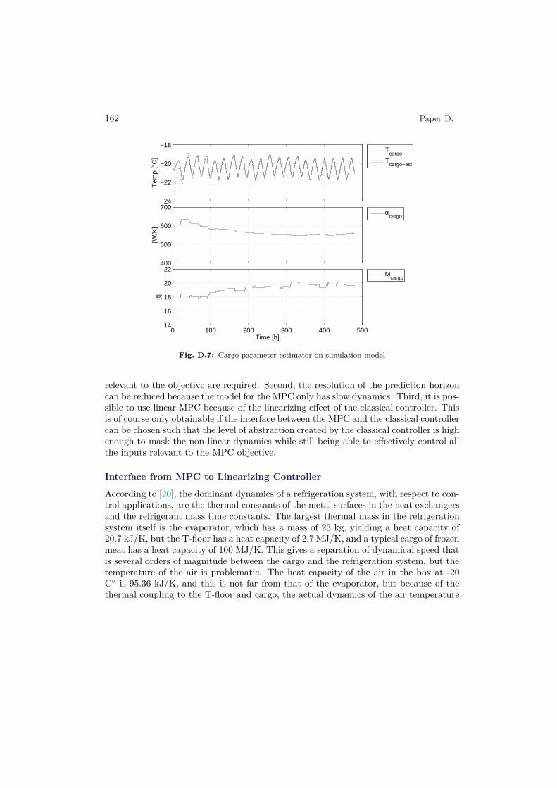
162 Paper D.
−24
−22
−20
−18T
emp
[°C
]
T
cargo
Tcargo−est
400
500
600
700
[W/K
]
α
cargo
0 100 200 300 400 50014
16
18
20
22
Time [h]
[t]
M
cargo
Fig. D.7: Cargo parameter estimator on simulation model
relevant to the objective are required. Second, the resolution of the prediction horizoncan be reduced because the model for the MPC only has slow dynamics. Third, it is pos-sible to use linear MPC because of the linearizing effect of the classical controller. Thisis of course only obtainable if the interface between the MPC and the classical controllercan be chosen such that the level of abstraction created by the classical controller is highenough to mask the non-linear dynamics while still being able to effectively control allthe inputs relevant to the MPC objective.
Interface from MPC to Linearizing Controller
According to [20], the dominant dynamics of a refrigeration system, with respect to con-trol applications, are the thermal constants of the metal surfaces in the heat exchangersand the refrigerant mass time constants. The largest thermal mass in the refrigerationsystem itself is the evaporator, which has a mass of 23 kg, yielding a heat capacity of20.7 kJ/K, but the T-floor has a heat capacity of 2.7 MJ/K, and a typical cargo of frozenmeat has a heat capacity of 100 MJ/K. This gives a separation of dynamical speed thatis several orders of magnitude between the cargo and the refrigeration system, but thetemperature of the air is problematic. The heat capacity of the air in the box at -20C◦ is 95.36 kJ/K, and this is not far from that of the evaporator, but because of thethermal coupling to the T-floor and cargo, the actual dynamics of the air temperature

2. Methods 163
ContainerParameter
Estimator
MPCConstraint
Calculator
Model Parameters
Measurements
Classical
Controller
Fig. D.8: Overall Controller Block Diagram
are considerably slower. The important factor is the response from the supply tempe-rature Tsup to the return temperature Tret, and because the air has to flow over boththe T-floor and the cargo, the response is slowed considerably. The T-floor alone issufficient to leave a comfortable gap in dynamical speeds between the dynamics thatmust be controlled by the MPC and the non-linear refrigeration system dynamics.
The cooling capacity Qcool is chosen as the reference from the MPC to the classicalcontroller because it has a direct and nearly linear effect on the cargo temperature. Theproposed controller set up is shown in Figure D.9.
ContainerLinearizingController
MPC
∫
ConstraintCalculator
+
+
-
Cooling CapacityCalculation
Measured Cooling Capacity
Cooling Capacity Reference
Model Parameters
Set-point
+
Fan SpeedParameter Estimator
Measurements
Measurements
Fig. D.9: Controller Block Diagram
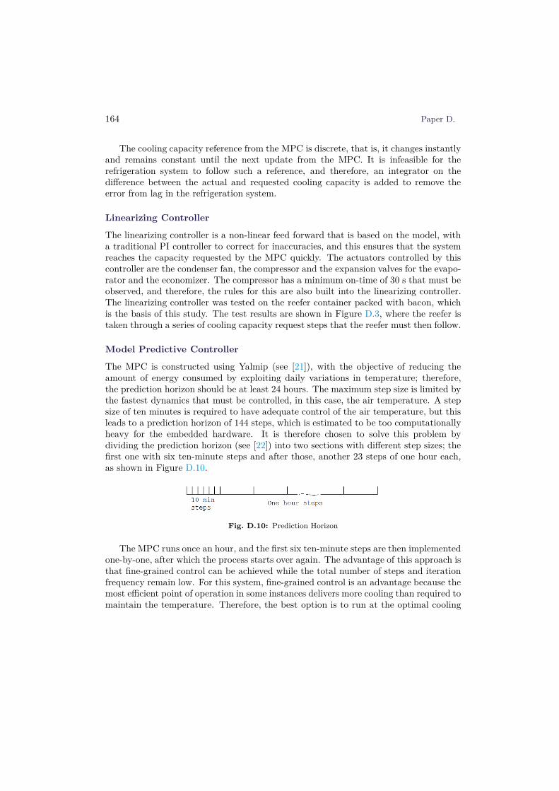
164 Paper D.
The cooling capacity reference from the MPC is discrete, that is, it changes instantlyand remains constant until the next update from the MPC. It is infeasible for therefrigeration system to follow such a reference, and therefore, an integrator on thedifference between the actual and requested cooling capacity is added to remove theerror from lag in the refrigeration system.
Linearizing Controller
The linearizing controller is a non-linear feed forward that is based on the model, witha traditional PI controller to correct for inaccuracies, and this ensures that the systemreaches the capacity requested by the MPC quickly. The actuators controlled by thiscontroller are the condenser fan, the compressor and the expansion valves for the evapo-rator and the economizer. The compressor has a minimum on-time of 30 s that must beobserved, and therefore, the rules for this are also built into the linearizing controller.The linearizing controller was tested on the reefer container packed with bacon, whichis the basis of this study. The test results are shown in Figure D.3, where the reefer istaken through a series of cooling capacity request steps that the reefer must then follow.
Model Predictive Controller
The MPC is constructed using Yalmip (see [21]), with the objective of reducing theamount of energy consumed by exploiting daily variations in temperature; therefore,the prediction horizon should be at least 24 hours. The maximum step size is limited bythe fastest dynamics that must be controlled, in this case, the air temperature. A stepsize of ten minutes is required to have adequate control of the air temperature, but thisleads to a prediction horizon of 144 steps, which is estimated to be too computationallyheavy for the embedded hardware. It is therefore chosen to solve this problem bydividing the prediction horizon (see [22]) into two sections with different step sizes; thefirst one with six ten-minute steps and after those, another 23 steps of one hour each,as shown in Figure D.10.
Fig. D.10: Prediction Horizon
The MPC runs once an hour, and the first six ten-minute steps are then implementedone-by-one, after which the process starts over again. The advantage of this approach isthat fine-grained control can be achieved while the total number of steps and iterationfrequency remain low. For this system, fine-grained control is an advantage because themost efficient point of operation in some instances delivers more cooling than required tomaintain the temperature. Therefore, the best option is to run at the optimal cooling

2. Methods 165
capacity for shorter time, and by dividing the first hour into six smaller steps, theeffective minimum capacity that can be delivered per hour is reduced to a level that ismore suitable for this application.
Cost Calculation and Constraint Setup
The evaporator fan circulates the air that moves energy from the box to the evaporator;therefore, it is required to run while the compressor is turned on. The power consump-tion of the fan has an impact on the cost of running the system in two ways: there is thedirect power driving the fan and the heat generated by the fan that must be removedagain by the refrigeration system. The fan speed is controlled in discrete steps; thus,it is important to model this behaviour in the actuator constraints of the controller.This is performed by declaring the fan speed as a binary variable, which transforms theproblem to a mixed-integer program. The resulting constraint is shown in Equation(D.19).
The fan speed variable Vfan is 1 when the fan is turned on, and Qmin and Qmax
are the constraints on the cooling capacity, which are calculated based on the currentoperating point. From Equation (D.19), it is obvious that Qcool is required to be zerowhen the fan is turned off, and it is constrained by Qmin and Qmax when the fan isturned on.
The maximal cooling capacity of the refrigeration system is dependent on suctionpressure and thus the temperature in the box, and therefore, Qmax and Qmin fromEquation D.19 must be calculated from the box temperature. This is performed usingmanufacturer data given as polynomials according to [23].
In many real systems, we encounter a non-linear cost on a control input, typicallydue to decreasing efficiency as the speed of an actuator increases. This is also the casefor this system, but only to a limited degree for the compressor. The largest change inCOP for the refrigeration system is dependent on the ambient temperature because ithas a strong coupling to the discharge pressure, which is a determining factor on theefficiency of the compressor. In Figure D.11, the COP of the system is shown for a fixedsetpoint of -20◦C and varying cooling capacity and ambient temperature is shown.
The dotted line is the COP of the system when the compressor is running in PWMmode, where the compressor is stopped and started with a duty cycle that matches therequired cooling capacity. It is necessary to perform this when the cooling capacityrequired to maintain the setpoint in the container is lower than that provided by therefrigeration system at the lowest possible compressor speed. The reason for the sharpdecline of COP in PWM mode is that the evaporator fan continues running while thecompressor is off, and therefore, the contribution from the fan compared to the coolingcapacity is increased as the duty cycle approaches zero. The expression for the COP in

166 Paper D.
0 1 2 3 4 5 6 7 80
0.5
1
1.5
2
2.5
3
3.5
4
Tamb = 0°C
Tamb = 10°C
Tamb = 20°C
Tamb = 30°C
Tamb = 40°C
Tamb = 50°C
CO
P [−
]
Cooling Capacity [kW]
COP at setpoint −20°C
COPPWM
COPCOP
MAX
Fig. D.11: The COP of the refrigeration system at varying ambient temperatures
PWM mode is given in Equation (D.17)
COPP W M =D · Qcool−min − Qfan
D · Pcpr−min + Qfan
(D.17)
where D is the duty cycle, Qcool−min is the cooling capacity at minimum compressorspeed, Pcpr−min is the consumed compressor power at minimum compressor speed, andQfan is the power consumed by the fan. The ambient temperature has a substantialimpact on both the level and the shape of the COP curve, and to effectively exploitthis property, the objective of the MPC must accurately reflect the cost over the lengthof the prediction horizon. This requires knowledge of the future ambient temperature,which is not available; therefore, the predictor outlined in Section 2.2 is used. Thepredicted ambient temperature is used to select the appropriate COP curve, whichmust be converted to an affine cost that reflects the shape of the COP curve. TheCOP curve shown here has 9 points because it is generated by simulating the model,as described in Section 2.1, to steady state at fixed compressor speeds from 20 Hz to110 Hz in increments of 10 Hz. For the MPC, a set of COP curves is generated athigher resolution for the ambient temperature to ensure optimal conditions for the cost

2. Methods 167
optimization.A linear solver is used, and therefore, the COP data are converted to a series of
linear segments in the form y = ax + b such that they may be used in an epigraphrepresentation of the cost of running the compressor in the objective function. Theobjective and constraints are listed in Equations (D.18) to (D.27):
Objective:Pc(k) + Vfan(k) · 195 + Ts(k) · 104 (D.18)
Constraints:
Vfan(k) · Qmin(k) <= Qcool(k) <= Vfan(k) · Qmax(k) (D.19)
Qcool(k) · a1(k) + b1(k) <= Pc(k) (D.20)
Qcool(k) · a2(k) + b2(k) <= Pc(k) (D.21)
Qcool(k) · a3(k) + b3(k) <= Pc(k) (D.22)
Qcool(k) · a4(k) + b4(k) <= Pc(k) (D.23)
Vfan−min <= Vfan(k) <= 1 (D.24)
0 <= Ts(k), (D.25)
Tcargo−min − Ts(k) <= Tcargo(k) <= Tcargo−max + Ts(k), (D.26)
Tair(k) < Tair−max + Ts(k) (D.27)
The objective function shown in Equation (D.18) reflects the power used by thecontainer, expressed by the first and second terms, where Pc is the power used by thecompressor and condenser fan and Vfan(k)·195 is the power consumed by the evaporatorfans. The constraints given in Equations (D.20) to (D.23) are the linear approximationof the convex COP, where the parameters an(k) and bn(k) are derived from the COPcurve that matches the predicted ambient temperature at the time of the solution point,which results in a cost for the compressor that forms a surface with cooling capacity onone axis and time on the other.
The third term of the objective, the slack variable Ts, is the cost of violating theconstraints for cargo and air temperatures, which are defined in Equation (D.26) and(D.27). It ensures that the controller will keep running and produce solutions in theevent that one of the temperature constraints is violated. The cost of violating theconstraint is very high, and therefore, the controller will prioritize getting back insidethe constraints over all other objectives, and this is the desired behaviour.
It is not expected that the constraints will be violated under normal operation, buta violation could occur if the ambient conditions of the reefer change suddenly. Becausethe MPC is recalculated only once every hour, the applied cooling might be incorrectfor up to an hour; however, for frozen cargo, this is not critical. When reefers areunloaded from the ship, they are unpowered and may remain so for up to four hourswhile being transported by truck. For chilled cargo, it is critical not to cause chill

168 Paper D.
injuries by injecting air that is too cold into the cargo hold, and if the weather suddenlychanges from sunshine to rain, this situation might occur. Therefore, this controllerwould need to be supervised and the MPC recalculated ahead of time if the constraintswere violated to ensure adequate disturbance rejection.
The temperature constraint that has been selected for the cargo is Tset±0.25 K,which ensures that the variation in cargo temperature remains small, thereby reducingthe risk of damaging the cargo. The model used for the controller lumps the entire cargointo one large volume, but in reality, the temperature distribution inside the containeris non-uniform; see [10]. Therefore, the air temperature has been constrained to Tset+2K because this will ensure that the air is cooled and circulated regularly, which preventsthe formation of local hot-spots.
3 Results
The objective of the experiments conducted in this work is to identify potential reduc-tions in energy consumption by introducing modern control methods, and two differentscenarios are investigated at three different ambient temperatures in an attempt to mapthe energy savings potential. The traditional approach for controlling the evaporatorfan is that it must always be running because the measurement of the cargo tempera-ture is performed indirectly through the return air temperature, and this measurementbecomes invalid when the fans are turned off. However, with the cargo estimator, itis possible to turn off the fans and use the estimate of the air and cargo temperatureinstead, which results in a substantial reduction in consumed energy. It is however in-teresting to know the fraction of the reduction that comes from cooling storage in thecargo and how much that comes from savings on the fans. Therefore, the first scenariouses the MPC with the fans forced to be always on, and the second scenario allowsthe MPC to control both the fans and the cooling capacity. The references used in theexperiments are simulations using the same linearizing controller as for the MPC butwith a traditional PI controller for generation of the cooling capacity reference. In Fig-ure D.12, a section of the simulation results for the reference and the two test scenariosare shown. The two panels on top are the reference simulation, the two panels in themiddle are the scenario where the fans are always on, and the two panels in the bottomare the scenario where the controller is allowed to turn off the fans. In the referencesimulation, the fans are running continuously and the controller keeps the cargo and airtemperature close to the setpoint. The compressor is running in PWM mode, and itcan be observed that the duty cycle and cooling request are increased at high ambienttemperatures to compensate for the higher influx of heat into the cargo hold.
For the scenario where the fans are always on, it can be observed that the MPCuses the cargo’s thermal inertia, allowing the air and cargo temperature to rise to itsupper constraint during the period where the ambient temperature is at its highest.The compressor is running in PWM most of the time because there is nothing to gain
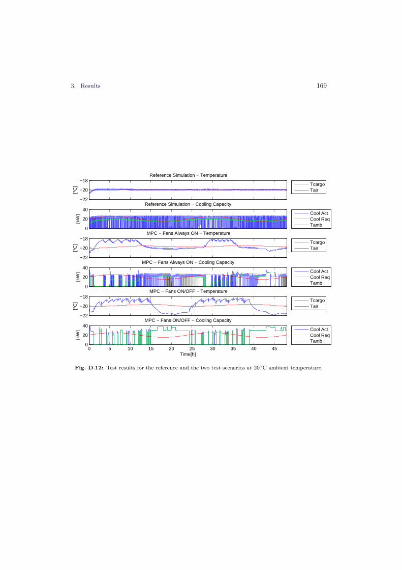
3. Results 169
−22
−20
−18
[°C
]
Reference Simulation − Temperature
TcargoTair
0
20
40
[kW
]
Reference Simulation − Cooling Capacity
Cool ActCool ReqTamb
−22
−20
−18
[°C
]
MPC − Fans Always ON − Temperature
TcargoTair
0
20
40
[kW
]
MPC − Fans Always ON − Cooling Capacity
Cool ActCool ReqTamb
−22
−20
−18
[°C
]
MPC − Fans ON/OFF − Temperature
TcargoTair
0 5 10 15 20 25 30 35 40 450
20
40
Time[h]
[kW
]
MPC − Fans ON/OFF − Cooling Capacity
Cool ActCool ReqTamb
Fig. D.12: Test results for the reference and the two test scenarios at 20◦C ambient temperature.

170 Paper D.
by running the compressor faster, at a lower efficiency, if it is not possible to turn offthe fans for a longer period afterwards.
In the last scenario, the fans are turned off when the compressor is not running, andthe compressor is now running at a higher capacity, which allows the compressor andfans to be turned off for longer periods, thus saving power. During the periods of highambient temperature, the compressor is only turned on to keep the air temperaturebelow the upper limit while the cargo temperature is slowly increasing, and this showsthat the controller behaves as intended.
The power savings found in the six tests are listed in Table D.1.From the results, it is clear that the potential power savings are highly dependent on
the operating conditions, and the reason for this is found in the COP curves in FigureD.11 and in the way the refrigeration system was designed. During normal operationof the container, when the cargo is at its setpoint, the system is typically running at afraction of the cooling capacity that is available because the system is designed to beable to cool a hot cargo within a reasonable amount of time. However, the system isalso most efficient when it is running at low capacity because the losses in the systemare smaller at low capacity. The COP curve for the compressor alone is monotonicallydecreasing as the speed increases, but when the power from the fans is added, the COPcurves shown in Figure D.11 with a maximum in the lower capacity range emerge.
Ambient Temperature Fans Always ON Fans ON/OFF10 ± 5◦C 2.53% 21.9%20 ± 5◦C 3.07% 11.1%30 ± 5◦C 2.70% 3.96%
Table D.1: Results from the different test scenarios.
This means that when the amount of cooling required to maintain the setpoint inthe cargo hold matches the most efficient capacity, the potential energy reduction frombeing able to turn off the fans is low. This is reflected by the results that show thatthe energy savings decrease as the ambient temperature increases. When the mostefficient mode of operation is running the fans continuously, the cargo may still beused as a cooling storage, and therefore, there will always be a gain from using thiscontrol strategy. In the present experiments, potential savings between 2.5% and 3%are possible with a 10 K variation in ambient temperature. With a consumption of 8.9MW for all the containers on a ship, a 2.5% reduction yields 403.7 GJ over a 21 day trip,which is approximately 10000 kg of heavy fuel oil. The six tests presented here showthat there is a large difference in potential savings depending on the cooling demand.Therefore, further tests should be conducted to test the entire range of operation ofthe container. It is expected that the largest savings will be found where the differencebetween the temperature setpoint and ambient temperature is low because, in this case,the majority of the heat input to the cargo hold is from the evaporator fans. This means

4. Conclusion 171
that switching off the fans yields a large decrease in the required cooling capacity andresults in relatively large savings on both the fan and the compressor. Therefore, it isexpected that it is possible to save a larger percentage of the power for shipments offruits and vegetables that run at a higher setpoint.
4 Conclusion
In this study, a model predictive controller that reduced the power consumption of arefrigerated container by turning off the cargo hold fans when they were not neededand by using the cargo thermal inertia to store cooling was presented. Simulationexperiments were performed using a detailed model of the refrigeration system at threedifferent ambient temperatures, with savings in power consumption found to be upto 21% depending on the ambient temperature. It is expected that larger savings arepossible for cargoes that requires a higher setpoint. The largest savings were found to bepossible only if the controller could control the fans and turn them off when they were notneeded. An estimator for cargo temperature, heat capacity, and heat transfer value wasdeveloped and used to update the MPC on-line, thereby enabling optimal exploitation ofthe available thermal inertia while keeping the cargo temperature within its constraints.The controller was divided into two layers, with the MPC on top providing a coolingpower request to a linearizing controller, which handled the faster non-linear dynamics ofthe refrigeration system. A prediction horizon with varying step sizes led to a reductionin the computational demand from the MPC.
References
[1] Marinelink, “World trade in perishable cargo to grow,”2013. [Online]. Available: http://www.marinelink.com/news/article/world-trade-in-perishable-cargo-to-grow/328311.aspx
[2] Container-Handbook, “8.1.2 actual power consumption,” 2009. [Online]. Avail-able: http://www.containerhandbuch.de/chb_e/wild/index.html?/chb_e/wild/wild_08_01_02.html
[3] R. G. M. van der Sman and G. J. C. Verdijck, “Model predictions andcontrol of conditions in a ca-reefer container,” in ISHS Acta Horticulturae 600:VIII International Controlled Atmosphere Research Conference, AgrotechnologicalResearch Institute ATO, P.O. box 17, 6700 AA Wageningen, the Netherlands,2003, pp. 163–171. [Online]. Available: http://www.actahort.org/members/showpdf?booknrarnr=600_20
172 References
[4] R. Halvgaard, N. K. Poulsen, H. Madsen, and J. B. Jorgensen, “Economic modelpredictive control for building climate control in a smart grid,” in Innovative SmartGrid Technologies (ISGT), 2012 IEEE PES, IEEE. http://orbit.dtu.dk/fedora/objects/orbit:74519/datastreams/file_6543920/content, 2012, pp. 1–6.
[5] Y. Ma and F. Borrelli, “Fast stochastic predictive control for building temperatureregulation,” in American Control Conference (ACC), 2012, June 2012, pp. 3075–3080. doi:10.1109/ACC.2012.6315347
[6] F. Oldewurtel, A. Parisio, C. Jones, M. Morari, D. Gyalistras, M. Gw-erder, V. Stauch, B. Lehmann, and K. Wirth, “Energy efficient building cli-mate control using stochastic model predictive control and weather predic-tions,” in American Control Conference (ACC), 2010, June 2010, pp. 5100–5105.doi:10.1109/ACC.2010.5530680
[7] J. E. Braun, “Reducing energy costs and peak electrical demand through optimalcontrol of building thermal mass,” ASHRAE Transactions, pp. 264–273, 1990.
[8] J. E. Braun and R. W. H. Laboratories, “Load control using building thermal mass,”in Transactions of the ASME Vol. 125, 2003, pp. 292–301. doi:10.1115/1.1592184
[9] K. Vinther, H. Rasmussen, R. Izadi-Zamanabadi, J. Stoustrup, and A. Alleyne,“A learning based precool algorithm for utilization of foodstuff as thermal energystorage,” in Control Applications (CCA), 2013 IEEE International Conference on,Aug 2013, pp. 314–321. doi:10.1109/CCA.2013.6662777
[10] G. J. C. Verdijck, “Model-based product quality control applied to climatecontrolled processing of agro-material,” 2003. [Online]. Available: http://alexandria.tue.nl/extra2/200310443.pdf
[11] Wageningen, “Agrotechnology & food sciences group, quest-leaflet,”2015. [Online]. Available: https://www.wageningenur.nl/upload_mm/d/6/b/2b3cd77e-4c34-4a62-95a9-1142267427de_Questleaflet2008.pdf
[12] J. d. Boogaard, G.J.P.M. van den; Kramer, “Quest: Quality and energy in storageand transport of agro-materials, final public report,” Wageningen Agrotechnology& Food Sciences Group, (Rapport / AFSG 657), 2006.
[13] A. Jakobsen, B. Rasmussen, and M. Skovrup, “Development of energy optimalcapacity control in refrigeration systems,” in Proceedings of 2000 International Re-frigeration Conference. Purdue University, Indiana, USA: http://docs.lib.purdue.edu/cgi/viewcontent.cgi?article=1498&context=iracc, 2000, pp. 329–336.
[14] MCI, “Maersk container industry, starcool refrigerated container specifications,”2013. [Online]. Available: http://www.maerskbox.com/
References 173
[15] K. Sørensen, M. Skovrup, L. Jessen, and J. Stoustrup, “Modular modelling of areefer container,” Accepted - In press, International Journal of Refrigeration, 2015.[Online]. Available: http://authors.elsevier.com/sd/article/S0140700715000766.doi:10.1016/j.ijrefrig.2015.03.017
[16] “Star cool reefer specification,” 2015. [Online]. Available: http://ipaper.ipapercms.dk/MCI/Brochures/MarkQ/
[17] “Specific heats of common food and foodstuff,” 2015. [Online]. Available: http://www.engineeringtoolbox.com/specific-heat-capacity-food-d_295.html
[18] S. Engell, “Feedback control for optimal process operation,” Journalof Process Control, vol. 17, no. 3, pp. 203 – 219, 2007. [Online].Available: http://www.sciencedirect.com/science/article/pii/S0959152406001326.doi:10.1016/j.jprocont.2006.10.011
[19] L. F. S. Larsen, “Model based control of refrigeration systems,” 2005. [Online].Available: http://www.control.aau.dk/~jakob/phdStudents/lfslThesis.pdf
[20] B. Rasmussen, A. Musser, and A. Alleyne, “Model-driven system identification oftranscritical vapor compression systems,” IEEE Transactions on Control SystemsTechnology, vol. 13, no. 3, pp. 444–451, 2005. doi:10.1109/TCST.2004.839572
[21] J. Löfberg, “Yalmip is a modelling language for defining and solving advancedoptimization problems,” 2009. [Online]. Available: http://users.isy.liu.se/johanl/yalmip/
[22] U. Halldorsson, M. Fikar, and H. Unbehauen, “Nonlinear predictive control withmultirate optimisation step lengths,” IEE Proceedings - Control Theory and Appli-cations, vol. 152, no. 3, pp. 273–285, 2005. doi:10.1049/ip-cta:20041310
[23] BS, “British standard/en 12900, refrigerant compressors. rating conditions, toler-ances and presentation of manufacturer’s performance data,” ISBN: 0 580 32694 2,2005.


![Automating Reefer Monitoring in Terminalswebinar-1]-automating-reefer... · •No terminal solution for full site coverage Stable and Proven Reefer Monitoring Solution RMM Slave PowerLine](https://static.fdocuments.in/doc/165x107/5dd0cf52d6be591ccb62ce92/automating-reefer-monitoring-in-terminals-webinar-1-automating-reefer-ano.jpg)