Model-Based Clustering of High-Dimensional Data:Variable Selection versus Facet DeterminationI

Leonard K. M. Poona, Nevin L. Zhanga, Tengfei Liua, April H. Liua

aDepartment of Computer Science and Engineering, The Hong Kong University of Science and Technology, Hong Kong,China

Abstract

Variable selection is an important problem for cluster analysis of high-dimensional data. It is also adifficult one. The difficulty originates not only from the lack of class information but also the fact thathigh-dimensional data are often multifaceted and can be meaningfully clustered in multiple ways. In such acase the effort to find one subset of attributes that presumably gives the “best” clustering may be misguided.It makes more sense to identify various facets of a data set (each being based on a subset of attributes),cluster the data along each one, and present the results to the domain experts for appraisal and selection.In this paper, we propose a generalization of the Gaussian mixture models and demonstrate its ability toautomatically identify natural facets of data and cluster data along each of those facets simultaneously. Wepresent empirical results to show that facet determination usually leads to better clustering results thanvariable selection.

Keywords: Model-based clustering, Facet determination, Variable selection, Latent tree models, Gaussianmixture models

1. Introduction

Variable selection is an important issue for cluster analysis of high-dimensional data. The cluster struc-ture of interest to domain experts can often be best described using a subset of attributes. The inclusion ofother attributes can degrade clustering performance and complicate cluster interpretation. Recently thereis a growing interest in the issue [2, 3, 4]. This paper is concerned with variable selection for model-basedclustering.

In classification, variable selection is a clearly defined problem, i.e., to find the subset of attributes thatgives the best classification performance. The problem is less clear for cluster analysis due to the lack ofclass information. Several methods have been proposed for model-based clustering. Most of them introduceflexibility into the generative mixture model to allow clusters to be related to subsets of (instead of all)attributes and determine the subsets alongside parameter estimation or during a separate model selectionphase. Raftery and Dean [5] consider a variation of the Gaussian mixture model (GMM) where the latentvariable is related to a subset of attributes and is independent of other attributes given the subset. A greedyalgorithm is proposed to search among those models for one with high BIC score. At each search step, twonested models are compared using the Bayes factor and the better one is chosen to seed the next searchstep. Law et al. [6] start with the Naıve Bayes model (i.e., GMM with diagonal covariance matrices) andadd a saliency parameter for each attribute. The parameter ranges between 0 and 1. When it is 1, theattribute depends on the latent variable. When it is 0, the attribute is independent of the latent variableand its distribution is assumed to be unimodal. The saliency parameters are estimated together with other

IAn earlier version of this paper appears in [1].Email addresses: lkmpoon@cse.ust.hk (Leonard K. M. Poon), lzhang@cse.ust.hk (Nevin L. Zhang), liutf@cse.ust.hk

(Tengfei Liu), aprillh@cse.ust.hk (April H. Liu)

Preprint submitted to International Journal of Approximate Reasoning July 18, 2012

model parameters using the EM algorithm. The work is extended by Li et al. [7] so that the saliency ofan attribute can vary across clusters. The third line of work is based on GMMs where all clusters share acommon diagonal covariance matrix, while their means may vary. If the mean of a cluster along an attributeturns out to coincide with the overall mean, then that attribute is irrelevant to cluster. Both Bayesianmethods [8, 9] and regularization methods [10] have been developed based on this idea.

Our work is based on two observations. First, while clustering algorithms identify clusters in data basedon the characteristics of data, domain experts are ultimately the ones to judge the interestingness of theclusters found. Second, high-dimensional data are often multifaceted in the sense that there may be multiplemeaningful ways to partition them. The first observation is the reason why variable selection for clusteringis such a difficult problem, whereas the second one suggests that the problem may be ill-conceived from thestart.

Instead of the variable selection approach, we advocate a facet determination approach. The idea is tosystematically identify all the different facets of a data set, cluster the data along each one, and presentthe results to the domain experts for appraisal and selection. The analysis would be useful if one of theclusterings is found interesting.

The difference between the two approaches can be elucidated by comparing their objectives. In variableselection, the aim is to find one subset of attributes that gives the “best” or “good” clustering result. Infacet determination, the aim is to find multiple subsets of attributes such that each subset gives meaningfulpartition of data. In other words, performing facet determination can be considered as performing multiplevariable selection simultaneously, without assuming that there is only a single “best” solution.

To realize the idea of facet determination, we generalize the GMMs to allow multiple latent variables.For computational tractability, we restrict that each attribute can be connected to only one latent variableand the relationships among the latent variables can be represented as a tree. The result is what we callpouch latent tree models (PLTMs). Analyzing data using a PLTM may result in multiple latent variables.Each latent variable represents a partition (clustering) of the data and is usually related primarily to onlya subset of attributes. Consequently, facets of data can be identified by those subsets of attributes.

Facet determination has been investigated under different designations in previous work. Two otherclasses of models have been considered. Galimberti and Soffritti [11] use a collection of GMMs, each on adisjoint subset of attributes, for facet determination. We refer to their method as the GS method. Themethod starts by obtaining a partition of attributes using variable clustering. A GMM is built on eachsubset of attributes and the collection of GMMs is evaluated using the BIC score. To look for the optimalpartition of attributes, the method repeatedly merges the two subsets of attributes that lead to the largestimprovement in the BIC score. It stops when no subsets can be merged to improve the score. Similar to theGS models, PLTMs can be considered as containing a collection of GMMs on disjoint subsets of attributes.However, the GMMs in PLTMs are connected by a tree structure, whereas those in the GS models aredisconnected.

Latent tree models (LTMs) [12, 13] are another class of models that have been used for facet determina-tion [14]. LTMs and PLTMs are much alike. However, LTMs include only discrete variables and can handleonly discrete data. PLTMs generalize LTMs by allowing continuous variables. As a result, PLTMs can alsohandle continuous data.

Two contributions are made in this paper. The first one is a new class of models in PLTMs, resultingfrom the marriage between GMMs and LTMs. PLTMs not only generalize GMMs to allow multiple latentvariables, but they also generalize LTMs for handling continuous data. The generalization of LTMs isinteresting for two reasons. First, it is desirable to have a tool for facet determination on continuous data.Second, the generalization is technically non-trivial. It requires new algorithms for inference and structurallearning.

The second contribution is that we compare the variable selection approach and the facet determinationapproach for model-based clustering. The two approaches have not been compared in the previous studieson facet determination [11, 14]. In this paper, we show that facet determination usually leads to betterclustering results than variable selection.

The rest of the paper is organized as follows. Section 2 reviews traditional model-based clusteringusing GMMs. PLTMs is then introduced in Section 3. In Sections 4–6, we discuss inference, estimation,

2

and structural learning for PLTMs. The empirical evaluation is divided into two parts. In Section 7, weanalyze real-world basketball data using PLTMs. We aim to demonstrate the effectiveness of using PLTMsfor facet determination. In Section 8, we compare PLTMs with other methods on benchmark data. Weaim to compare the facet determination approach and the variable selection approach. After the empiricalevaluation, we discuss related work in Section 9 and conclude in Section 10.

2. Background and Notations

In this paper, we use capital letters such as X and Y to denote random variables, lower case letters suchas x and y to denote their values, and bold face letters such as X, Y , x, and y to denote sets of variablesor values.

Finite mixture models are commonly used in model-based clustering [15, 16]. In finite mixture modeling,the population is assumed to be made up from a finite number of clusters. Suppose a variable Y is used toindicate this cluster, and variables X represent the attributes in the data. The variable Y is referred to asa latent (or unobserved) variable, and the variables X as manifest (or observed) variables. The manifestvariables X is assumed to follow a mixture distribution

P (x) =∑y

P (y)P (x|y).

The probability values of the distribution P (y) are known as mixing proportions and the conditional distri-butions P (x|y) are known as component distributions. To generate a sample, the model first picks a clustery according to the distribution P (y) and then uses the corresponding component distribution P (x|y) togenerate values for the observed variables.

Gaussian distributions are often used as the component distributions due to computational convenience.A Gaussian mixture model (GMM) has a distribution given by

P (x) =∑y

P (y)N (x|µy,Σy),

where N (x|µy,Σy) is a multivariate Gaussian distribution, with mean vector µy and covariance matrix Σy

conditional on the value of Y .The Expectation-Maximization (EM) algorithm [17] can be used to fit the model. Once the model is fit,

the probability that a data point d belongs to cluster y can be computed by

P (y|d) ∝ P (y)N (d|µy,Σy),

where the symbol ∝ implies that the exact values of the distribution P (y|d) can be obtained by using thesum

∑y P (y)N (d|µy,Σy) as a normalization constant.

The number G of components (or clusters) can be given manually or determined by model selectionautomatically. In the latter case, a score is used to evaluate a model with G clusters. The G that leads tothe highest score is then chosen as the estimated number of components. The BIC score has been empiricallyshown to perform well for this purpose [18].

3. Pouch Latent Tree Models

A pouch latent tree model (PLTM) is a rooted tree, where each internal node represents a latent variable,and each leaf node represents a set of manifest variables. All the latent variables are discrete, while all themanifest variables are continuous. A leaf node may contain a single manifest variable or several of them.Because of the second possibility, leaf nodes are called pouch nodes.1 Figure 1a shows an example of PLTM.

1In fact, PLTMs allow both discrete and continuous manifest variables. The leaf nodes may contain either a single discretevariable, a single continuous variable, or multiple continuous variables. For brevity, we focus on continuous manifest variablesin this paper.

3

(a) (b) (c)

Figure 1: (a) An example of PLTM. The latent variables are shown in shaded nodes. The numbers inparentheses show the cardinalities of the discrete variables. (b) Generative model for synthetic data. (c)GMM as a special case of PLTM.

y1 P (y1)s1 0.33s2 0.33s3 0.34

P (y2|y1)y2 y1 = s1 y1 = s2 y1 = s3s1 0.74 0.13 0.13s2 0.13 0.74 0.13s3 0.13 0.13 0.74

Table 1: Discrete distributions in Example 1.

In this example, Y1–Y4 are discrete latent variables, where Y1–Y3 have three possible values and Y4 hastwo. X1–X9 are continuous manifest variables. They are grouped into five pouch nodes, {X1, X2}, {X3},{X4, X5}, {X6}, and {X7, X8, X9}.

Before we move on, we need to explain some other notations. We use capital letter Π(V ) to indicate theparent variable of a variable V and lower case letter π(V ) to denote its value. Also, we reserve the use ofbold capital letter W for denoting the variables of a pouch node. When the meaning is clear from context,we use the terms ‘variable’ and ‘node’ interchangeably.

In a PLTM, the dependency of a discrete latent variable Y on its parent Π(Y ) is characterized by aconditional discrete distribution P (y|π(Y )).2 Let W be the variables of a pouch node with a parent nodeY = Π(W ). We assume that, given a value y of Y , W follows the conditional Gaussian distributionP (w|y) = N (w|µy,Σy) with mean vector µy and covariance matrix Σy. A PLTM can be written as a pairM = (m,θ), where m denotes the model structure and θ denotes the parameters.

Example 1. Figure 1b gives another example of PLTM. In this model, there are two discrete latent variablesY1 and Y2, each having three possible values {s1, s2, s3}. There are six pouch nodes, namely {X1, X2}, {X3},{X4}, {X5}, {X6}, and {X7, X8, X9}. The variables in the pouch nodes are continuous.

Each node in the model is associated with a distribution. The discrete distributions P (y1) and P (y2|y1),associated with the two discrete nodes, are given in Table 1.

The pouch nodes W are associated with conditional Gaussian distributions. These distributions haveparameters for specifying the conditional means µπ(W ) and conditional covariances Σπ(W ). For the fourpouch nodes with single variables, {X3}, {X4}, {X5}, and {X6}, these parameters have scalar values. Theconditional means µy for each of these variables are either −2.5, 0, and 2.5, depending on whether y = s1, s2,or s3, where y is the value of the corresponding parent variable Y ∈ {Y1, Y2}. The conditional covariances Σycan also have different values for different values of their parents. However, for simplicity in this example,we set Σy = 1,∀y ∈ {s1, s2, s3}.

2 The root node is regarded as the child of a dummy node with only one value, and hence is treated in the same way asother latent nodes.

4

Let p be the number of variables in a pouch node. The conditional means are specified by p-vectors andthe conditional covariances by p × p matrices. For example, the conditional means and covariances of thepouch node {X1, X2} are given by:

µy1 =

(−2.5,−2.5) : y1 = s1

(0, 0) : y1 = s2

(2.5, 2.5) : y1 = s3

and Σy1 =

(1 0.5

0.5 1

),∀y1 ∈ {s1, s2, s3}.

The conditional means and covariances are specified similarly for pouch node {X7, X8, X9}. The conditionalmeans for Xi, i ∈ {7, 8, 9}, can be -2.5, 0, or 2.5. The variance of any of these variables is 1, and thecovariance between any pair of these variables is 0.5.

PLTMs have a noteworthy two-way relationship with GMMs. On the one hand, PLTMs generalize thestructure of GMMs to allow more than one latent variable in a model. Thus, a GMM can be consideredas a PLTM with only one latent variable and one pouch node containing all manifest variables. As anexample, a GMM is depicted as a PLTM in Figure 1c, in which Y1 is a discrete latent variable and X1–X9

are continuous manifest variables.On the other hand, the distribution of a PLTM over the manifest variables can be represented by a

GMM. Consider a PLTM M . Suppose W 1, . . . ,W b are the b pouch nodes and Y1, . . . , Yl are the l latentnodes in M . Denote as X =

⋃bi=1W i and Y = {Yj : j = 1, . . . , l} the sets of all manifest variables and all

latent variables in M , respectively. The probability distribution defined by M over the manifest variablesX is given by

P (x) =∑y

P (x,y)

=∑y

l∏j=1

P (yj |π(Yj))

b∏i=1

N (wi|µπ(W i),Σπ(W i)) (1)

=∑y

P (y)N (x|µy,Σy). (2)

Equation 1 follows from the model definition. Equation 2 follows from the fact that Π(W i),Π(Yj) ∈ Yand the product of Gaussian distributions is also a Gaussian distribution. Equation 2 shows that P (x) is amixture of Gaussian distributions. Although it means that PLTMs are not more expressive than GMMs onthe distributions of observed data, PLTMs have two advantages over GMMs. First, numbers of parameterscan be reduced in PLTMs by exploiting the conditional independence between variables, as expressed bythe factorization in Equation 1. Second, and more important, the multiple latent variables in PLTMs allowmultiple clusterings on data.

Example 2. In this example, we compare the numbers of parameters in a PLTM and in a GMM. Consider adiscrete node and its parent node with c and c′ possible values, respectively. It requires (c−1)×c′ parametersto specify the conditional discrete distribution for this node. Consider a pouch node with p variables, andits parent variable with c′ possible values. This node has p× c′ parameters for the conditional mean vectors

and p(p+1)2 × c′ parameters for the conditional covariance matrices. Now consider the PLTM in Figure 1a

and the GMM in Figure 1c. Both of them define a distribution on 9 manifest variables. Based on the aboveexpressions, the PLTM has 77 parameters and the GMM has 164 parameters.

Given the same number of manifest variables, a PLTM may appear to be more complex than a GMM,due to a larger number of latent variables. However, this example shows that a PLTM can still require fewerparameters than a GMM.

The graphical structure of PLTMs looks similar to that of the Bayesian networks (BNs) [19]. In fact, aPLTM is different from a BN only because of the possibility of multiple variables in a single pouch node.It has been shown that any nonsingular multivariate Gaussian distribution can be converted to a complete

5

Gaussian Bayesian network (GBN) with an equivalent distribution [20]. Therefore, a pouch node can beconsidered as a shorthand notation of a complete GBN. If we convert each pouch node into a completeGBN, a PLTM can be considered as a conditional Gaussian Bayesian network (i.e., a BN with discretedistributions and conditional Gaussian distributions), or a BN in general.

Cluster analysis based on PLTMs requires learning PLTMs from data. It involves parameter estimationand structure learning. We discuss the former problem in Section 5, and the two problems as a whole inSection 6. Since parameter estimation involves inference on the model, we discuss this problem in the nextsection before the other two problems.

4. Inference

A PLTM defines a probability distribution P (X,Y ) over manifest variables X and latent variables Y .Consider observing values e for the evidence variables E ⊆ X. For a subset of variables Q ⊆ X ∪ Y , weare often required to compute the posterior probability P (q|e). For example, classifying a data point d toone of the clusters represented by a latent variable Y requires us to compute P (y|X = d).

Inference refers to the computation of the posterior probability P (q|e). It can be done on PLTMs simi-larly as the clique tree propagation on conditional GBNs [21]. However, due to the existence of pouch nodesin PLTMs, this propagation algorithm requires some modifications. The inference algorithm is discussed indetails in Appendix A.

The structure of PLTMs allows an efficient inference. Let n be the number of nodes in a PLTM, c be themaximum cardinality of a discrete variable, and p be the maximum number of variables in a pouch node.The time complexity of the inference is dominated by the steps related to message passing and incorporationof evidence on continuous variables. The message passing step requires O(nc2) time, since each clique hasat most two discrete variables due to the tree structure. Incorporation of evidence requires O(ncp3) time.

Suppose we have the same number of manifest variables. Since PLTMs generally has smaller pouchnodes than GMMs, and hence a smaller p, the term O(ncp3) shows that inference on PTLMs can be fasterthan that on GMMs. This happens even though PLTMs can have more nodes and thus a larger n.

5. Parameter Estimation

Suppose there is a data set D with N samples d1, . . . ,dN . Each sample consists of values for the manifestvariables. Consider computing the maximum likelihood estimate (MLE) θ∗ of the parameters for a given

PLTM structure m. We do this using the EM algorithm. The algorithm starts with an initial estimate θ(0)

and improves the estimate iteratively.Suppose the parameter estimate θ(t−1) is obtained after t − 1 iterations. The t-th iteration consists of

two steps, an E-step and an M-step. In the E-step, we compute, for each latent node Y and its parent Π(Y ),

the distributions P (y, π(Y )|dk,θ(t−1)) and P (y|dk,θ(t−1)) for each sample dk. This is done by the inferencealgorithm discussed in the previous section. For each sample k, let wk be the values of variables W of apouch node for the sample dk. In the M-step, the new estimate θ(t) is obtained as follows:

P (y|π(Y ),θ(t)) ∝N∑k=1

P (y, π(Y )|dk,θ(t−1))

µ(t)y =

∑Nk=1 P (y|dk,θ(t−1))wk∑Nk=1 P (y|dk,θ(t−1))

Σ(t)y =

∑Nk=1 P (y|dk,θ(t−1))(wk − µ(t)

y )(wk − µ(t)y )′∑N

k=1 P (y|dk,θ(t−1)),

where µ(t)y and Σ(t)

y here correspond to the distribution P (w|y,θ(t)) for node W conditional on its parentY = Π(W ). The EM algorithm proceeds to the (t+ 1)-th iteration unless the improvement of log-likelihood

logP (D|θ(t))− logP (D|θ(t−1)) falls below a certain threshold.

6

The starting values of the parameters θ(0) are chosen as follows. For P (y|π(Y ),θ(0)), the probabilitiesare randomly generated from a uniform distribution over the interval (0, 1] and are then normalized. The

initial values of µ(0)y are set to equal to a random sample from data, while those of Σ(0)

y are set to equal tothe sample covariance.

Like in the case of GMMs, the likelihood is unbounded in the case of PLTMs. This might lead to spuriouslocal maxima [15]. For example, consider a mixture component that consists of only one data point. If weset the mean of the component to be equal to that data point and set the covariance to zero, then the modelwill have an infinite likelihood on the data. However, even though the likelihood of this model is higher thansome other models, it does not mean that the corresponding clustering is better. The infinite likelihood canalways be achieved by trivially grouping one of the data points as a cluster. This is why we refer to thiskind of local maxima as spurious.

To mitigate this problem, we use a variant of the method by Ingrassia [22]. In the M-step of EM, we

need to compute the covariance matrix Σ(t)y for each pouch node W . We impose the following constraints

on the eigenvalues λ(t) of Σ(t)y : σ2

min/γ ≤ λ(t) ≤ σ2max × γ, where σ2

min and σ2max are the minimum and

maximum of the sample variances of the variables W and γ is a parameter for our method.

6. Structure Learning

Given a data set D, we aim at finding the model m∗ that maximizes the BIC score [23]:

BIC(m|D) = logP (D|m,θ∗)− d(m)

2logN,

where θ∗ is the MLE of the parameters and d(m) is the number of independent parameters in m. The firstterm is known as the likelihood term. It favors models that fit data well. The second term is known as thepenalty term. It discourages complex models. Hence, the BIC score provides a trade-off between model fitand model parsimoniousness.

We have developed a hill-climbing algorithm to search for m∗. It starts with a model m(0) that containsone latent node as root and a separate pouch node for each manifest variable as a leaf node. The latentvariable at the root node has two possible values. Suppose a model m(j−1) is obtained after j− 1 iterations.In the j-th iteration, the algorithm uses some search operators to generate candidate models by modifyingthe base model m(j−1). The BIC score is then computed for each candidate model. The candidate modelm′ with the highest BIC score is compared with the base model m(j−1). If m′ has a higher BIC scorethan m(j−1), m′ is used as the new base model m(j) and the algorithm proceeds to the (j + 1)-th iteration.Otherwise, the algorithm terminates and returns m∗ = m(j−1) (together with the MLE of the parameters).

We now describe the search operators used. There are four aspects of the structure m, namely, thenumber of latent variables, the cardinalities of these latent variables, the connections between variables,and the composition of pouches. The search operators used in our hill-climbing algorithm modify all theseaspects to effectively explore the search space. There are totally seven search operators. Five of them areborrowed from Zhang and Kocka [24], while two of them are new for PLTMs.

We first described the five operators borrowed from others. A node introduction (NI) operator involvesone latent node Y and two of its neighbors. It creates a new model by introducing a new latent node Ynew tomediate between Y and the two neighbors. The cardinality of Ynew is set to be that of Y . A node deletion(ND) operator is the opposite of NI. It involves two neighboring latent nodes Y and Ydelete. It creates a newmodel by deleting Ydelete and making all neighbors of Ydelete (other than Y ) neighbors of Y . Given a latentvariable in PLTM, a state introduction (SI) operator creates a new model by adding a state to the domainof the variable. A state deletion (SD) operator does the opposite. A node relocation (NR) involves a nodeV , one of its latent node neighbors Yorigin and another latent node Ydest. The node V can be a latent nodeor a pouch node. The NR operator creates a new model by relocating V to Ydest, i.e., removing the linkbetween V and Yorigin and adding a link between V and Ydest. Figure 2 gives some examples of the use ofNI, ND, and NR operators.

7

(a) m1 (b) m2 (c) m3

Figure 2: Examples of applying the node introduction, node deletion, and node relocation operators. Intro-ducing Y3 to mediate between Y1, {X4, X5} and {X6} in m1 gives m2. Relocating {X4, X5} from Y3 to Y2in m2 gives m3. In reverse, relocating {X4, X5} from Y2 to Y3 in m3 gives m2. Deleting Y3 in m2 gives m1.

(a) m1 (b) m2 (c) m3

Figure 3: Examples of applying the pouching and unpouching operators. Pouching {X4} and {X5} in m1

gives m2, and pouching {X4, X5} and {X6} in m2 gives m3. In reverse, unpouching X6 from {X4, X5, X6}in m3 gives m2, and unpouching X5 from {X4, X5} gives m1.

The two new operators are pouching (PO) and unpouching (UP) operators. The PO operator creates anew model by combining a pair of sibling pouch nodesW 1 andW 2 into a new pouch nodeW po = W 1∪W 2.The UP operator creates a new model by separating one manifest variable X from a pouch node W up,resulting in two sibling pouch nodes W 1 = W up\{X} and W 2 = {X}. Figure 3 shows some examples ofthe use of these two operators.

The purpose of the PO and UP operators is to modify the conditional independencies entailed by themodel on the variables of the pouch nodes. For example, consider the two models m1 and m2 in Figure 3.In m1, X4 and X5 are conditionally independent given Y3, i.e., P (X4, X5|Y3) = P (X4|Y3)P (X5|Y3). Inother words, covariance between X4 and X5 is zero given Y3. On the other hand, X4 and X5 need not beconditionally independent given Y3 in m2. The covariances between them are allowed to be non-zero in the2× 2 conditional covariance matrices for the pouch node {X4, X5}.

The PO operator in effect postulates that two sibling pouch nodes are correlated given their parentnode. It may improve the BIC score of the candidate model by increasing the likelihood term, when thereis some degree of local dependence between those variables on the empirical data. On the other hand, theUP operator postulates that one variable in a pouch node is conditionally independent from other variablesin the pouch node. It reduces the number of parameters in the candidate model and hence may improvethe BIC score by decreasing the penalty term. These postulates are tested by comparing the BIC scores ofthe corresponding models in each search step. The postulate that leads to the model with the highest BICscore is considered as most appropriate.

For the sake of computational efficiency, we do not consider introducing a new node to mediate betweenY and more than two of its neighbors. This restriction can be compensated by considering a restrictedversion of node relocation after a successful node introduction. Suppose Ynew is introduced to mediatebetween Y and its two neighbors. The restricted version of NR relocates one of the neighbors of Y (other

8

Figure 4: PLTM obtained on NBA data. The latent variables represent different clusterings on the players.They have been renamed based on our interpretation of their meanings. The abbreviations in these namesstand for: role (Role), general ability (Gen), technical fouls (T), disqualification (D), tall-player ability(Tall), shooting accuracy (Acc), and three-pointer ability (3pt).

than Ynew) to Ynew. The PO operator also has similar issue. Hence, after a successful pouching, we considera restricted version of PO. The restricted version combines the new pouch node resulting from PO with oneof its sibling pouch nodes.

The above explains the basic principles for the hill-climbing algorithm. However, the algorithm asoutlined above is inefficient and can handle only small data sets. We have developed acceleration techniquesthat make the algorithm efficient enough for some real-world applications. We leave these details in AppendixB.

7. Facet Determination on NBA Data

In the first part of our empirical study, we aim to demonstrate the effectiveness of facet determinationby PLTMs. Real-world basketball data were used in this study. The objective is to see whether the facetsidentified and the clusterings given by PLTM on this data set are meaningful or not. The analysis can beconsidered as effective if the facets and clusterings are meaningful in general. We interpret the clusteringsbased on our basic basketball knowledge.

The data contain seasonal statistics of National Basketball Association (NBA) players. They werecollected from 441 players who played in at least one game in the 2009/10 season.3 Each sample correspondsto one player. It includes the numbers of games played (games) and started (starts) by the player in thatseason. It also contains 16 other per game averages or seasonal percentages, including minutes (min),field goals made (fgm), field goal percentage (fgp), three pointers made (3pm), three pointer percentage(3pp), free throws made (ftm), free throw percentage (ftp), offensive rebounds (off), defensive rebounds(def), assists (ast), steals (stl), blocks (blk), turnovers (to), personal fouls (pf), technical fouls (tf), anddisqualifications (dq). In summary, the data set has 18 attributes and 441 samples.

7.1. Facets Identified

We built a PLTM on the data and the structure of the resulting model is shown in Figure 4. The modelcontains 7 latent variables. Each of the them identifies a different facet of data. The first facet consists ofattributes games and starts, which are related to the role of a player. The second one consists of attributesmin, fgm, ftm, ast, stl, and to, which are related to some general performance of a player. The third andfourth facets each contain only one attribute. They are related to tf and dq, respectively. The fifth facetcontains attributes blk, off, def, and pf. A player usually needs to jump higher than other players to geta block (blk) or a rebound (off or def). Therefore, the facet is mainly related to an aspect of performancein which taller players have an advantage. The sixth facet consists of two attributes ftp and fgp, which arerelated to the shooting accuracy. The last facet contains 3pm and 3pp, which are related to three pointers.

The facets identified consist mostly of related attributes. Hence, they appear to be reasonable in general.

3 The data were obtained from: http://www.dougstats.com/09-10RD.txt

9

Role P(Role) games starts

occasional players 0.32 29.1 2.0irregular starters 0.11 46.1 31.7regular substitutes 0.19 68.2 5.4regular players 0.13 75.8 32.8regular starters 0.25 76.0 73.7

overall 1.00 56.3 27.9

(a) Role of player (Role)

3pt P(3pt) 3pm 3pp

never 0.29 0.00 0.00seldom 0.12 0.08 0.26fair 0.17 0.33 0.28good 0.40 1.19 0.36extreme 0.02 0.73 0.64

overall 1.00 0.55 0.23

(b) Three-pointer ability (3pt)

Acc P(Acc) fgp ftp

low ftp 0.10 0.44 0.37low fgp 0.16 0.39 0.72high ftp 0.47 0.44 0.79high fgp 0.28 0.52 0.67

overall 1.00 0.45 0.71

(c) Shooting accuracy (Acc)

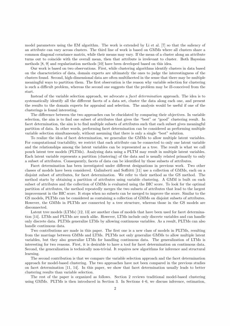
Table 2: Attribute means on three different facets on NBA data. The means are conditional on the specifiedlatent variables. The second columns show the marginal distributions of those latent variables. The lastrows show the unconditional means of the attributes. The clusters are named based on our interpretation.

7.2. Meanings of Clusters

To understand the meanings of the clusters, we may examine the mean values of attributes of eachcluster. We use three clusterings, Role, 3pt, and Acc, for illustration.

Table 2a shows the means of games and starts conditional on the clustering variable Role. Note thatthere are 82 games in a NBA season. We see that the mean value of games for the players in the first clusteris far below the overall mean. Hence, the first cluster contains players who played occasionally. The secondgroup of players also played less often than average, but they usually started in a game when they played.This may look counter-intuitive. However, the cluster probably refers to those players who had the calibreof starters but had missed part of the season due to injuries. The third group of players played often, butusually as substitutes (not as starters). The fourth group of players played regularly and sometimes startedin a game. The last group contains players who played and started regularly.

Table 2b shows the means of 3pm (three-pointer made) and 3pp (three-pointer percentage) conditionalon 3pt (three-pointer ability). The variable 3pt partitions players into five clusters. The first two clusterscontain players that never and seldom made a three-pointer, respectively. The next two clusters containsplayers that have fair and good three-pointer accuracies, respectively. The last group is an extreme case.It contains players shooting with unexpectedly high accuracy. As indicated by the marginal distribution, itconsists of only a very small proportion of players. This is possibly a group of players who had made somethree pointers during the sporadic games that they had played. The accuracy remained very high since theydid not play often.

Table 2c shows the means of fgp (field goal percentage) and ftp (free throw percentage) conditionalon Acc (shooting accuracy). The first three groups contain players of low ftp, low fgp, and high ftp,respectively. The fourth group of players had high fgp. However, those players also had below-average ftp.Both ftp and fgp are related to the shooting accuracies. Hence, one may expect that the two attributesshould be positively correlated and the fourth group may look unreasonable. However, the group is indeedsensible due to the following observation. Taller players usually stay closer to basket in games. Therefore,they take high-percentage shots more often and have higher field goal percentage. On the other hand, tallerplayers are usually poorer in making free throws and have lower free throw percentage. A typical example

10

Gen

Role poor fair goodoccasional players 0.81 0.19 0.00irregular starters 0.00 0.69 0.31regular substitutes 0.22 0.78 0.00regular players 0.00 0.81 0.19regular starters 0.00 0.06 0.94

(a) P (Gen|Role): relationship between general ability(Gen) and role (Role)

Acc

Tall low ftp low fgp high ftp high fgppoor 0.28 0.53 0.00 0.18fair 0.00 0.02 0.95 0.03good 0.00 0.00 1.00 0.00good big 0.11 0.04 0.00 0.86very good 0.00 0.00 0.14 0.86

(b) P (Acc|Tall): relationship between shooting accuracy (Acc)and tall-player ability (Tall)

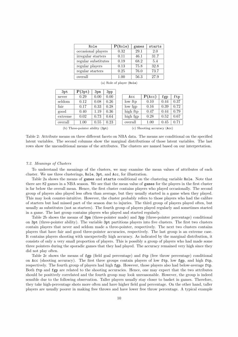
Table 3: Conditional distributions of Gen and Acc on NBA data.

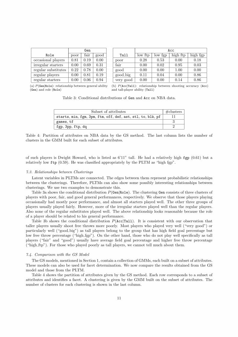
Subset of attributes #clustersstarts, min, fgm, 3pm, ftm, off, def, ast, stl, to, blk, pf 11games, tf 3fgp, 3pp, ftp, dq 2

Table 4: Partition of attributes on NBA data by the GS method. The last column lists the number ofclusters in the GMM built for each subset of attributes.

of such players is Dwight Howard, who is listed as 6’11” tall. He had a relatively high fgp (0.61) but arelatively low ftp (0.59). He was classified appropriately by the PLTM as “high fgp”.

7.3. Relationships between Clusterings

Latent variables in PLTMs are connected. The edges between them represent probabilistic relationshipsbetween the clusterings. Therefore, PLTMs can also show some possibly interesting relationships betweenclusterings. We use two examples to demonstrate this.

Table 3a shows the conditional distribution P (Gen|Role). The clustering Gen consists of three clusters ofplayers with poor, fair, and good general performances, respectively. We observe that those players playingoccasionally had mostly poor performance, and almost all starters played well. The other three groups ofplayers usually played fairly. However, more of the irregular starters played well than the regular players.Also none of the regular substitutes played well. The above relationship looks reasonable because the roleof a player should be related to his general performance.

Table 3b shows the conditional distribution P (Acc|Tall). It is consistent with our observation thattaller players usually shoot free throws more poorly. Most players who played very well (“very good”) orparticularly well (“good big”) as tall players belong to the group that has high field goal percentage butlow free throw percentage (“high fgp”). On the other hand, those who do not play well specifically as tallplayers (“fair” and “good”) usually have average field goal percentage and higher free throw percentage(“high ftp”). For those who played poorly as tall players, we cannot tell much about them.

7.4. Comparison with the GS Model

The GS models, mentioned in Section 1, contain a collection of GMMs, each built on a subset of attributes.These models can also be used for facet determination. We now compare the results obtained from the GSmodel and those from the PLTM.

Table 4 shows the partition of attributes given by the GS method. Each row corresponds to a subset ofattributes and identifies a facet. A clustering is given by the GMM built on the subset of attributes. Thenumber of clusters for each clustering is shown in the last column.

11

Compared to the results obtained from PLTM analysis, those from the GS method have three weaknesses.First, the facets found by the GS method appear to be less natural than those by PLTM analysis. Inparticular, attribute games can be related to many aspects of the game statistics. However, it is groupedtogether by the GS method with a less interesting attribute tf, which indicates the number of technical fouls,in the second subset. In the third subset, attributes fgp, 3pp, ftp are all related to shooting percentages.However, they are also grouped together with an apparently unrelated attribute dq (disqualifications). Thefirst subset lumps together a large number of attributes. This means it has missed some more specific andmeaningful facets that have been identified by PLTM analysis.

The second weakness is related to the numbers of clusters given by the GS method. One the one hand,there are a large number of clusters on the first subset. This makes it difficult to comprehend the clustering,especially with many attributes in this subset. On the other hand, there are only few clusters on the secondand third subsets. This means some subtle clusters found in PLTM analysis were not found by the GSmethod. The third weakness is inherent in the structure of the GS models. Since disconnected GMMs areused, the latent variables are assumed to be independent. Consequently, the GS models cannot show thosepossibly meaningful relationships between the clusterings as PLTMs do.

7.5. Discussions

The results presented above in general show that PLTM analysis identified reasonable facets and suggestthat it gave meaningful clusterings on those facets. We also see that better results were obtained fromPLTM analysis than the GS method. Therefore, we conclude that PLTMs can perform facet determinationeffectively on NBA data.

If we think about how basketball games are played, we can expect that the heterogeneity of players canoriginate from various aspects, such as positions of the players, their competence on their correspondingpositions, or their general competence. As our results show, PLTM analysis identified these different facetsfrom the NBA data and allowed users to partition data based on them separately. If traditional clusteringmethods are used, only one clustering can be obtained, regardless of whether variable selection is used ornot. Therefore, some of the facets cannot be identified by the traditional methods.

The number of attributes in NBA data may be small relatively to those data available nowadays. Nev-ertheless, we can still identify multiple facets and obtain multiple meaningful clusterings from the data. Wethus can expect real-world data with higher dimensions are also multifaceted. Consequently, it is in generalmore appropriate to use the facet determination approach with PLTMs than the variable selection selectionapproach for clustering high-dimensional data.

8. Facet Determination versus Variable Selection

In the previous section, we have demonstrated that multiple meaningful clusters can be found on a dataset. In such cases, variable selection methods are inadequate in the sense they can produce only singleclustering solutions and thus cannot identify all the meaningful clusterings. However, it is still possiblethat the single clustering produced by a variable selection method is more interesting to users than all theclusterings produced by a facet determination method.

In the second part of the empirical study, we aim to address this issue and compare the two approachesfor clustering. We want to see which method can produce the most interesting clustering. Due to the lackof domain experts, we use data with class labels. We assume that the partition indicated by the class labelsis the partition most interesting to users on a data set. The method that can produce a partition closest tothe class partition is deemed to be the best method in this study.

8.1. Data Sets and Methods

We used both synthetic and real-world data sets in this study. The synthetic data were generated fromthe model described in Example 1, of which the variable Y1 is designated as the class variable. The real-world data sets were borrowed from the UCI machine learning repository.4 We chose 9 labeled data sets

4 http://www.ics.uci.edu/~mlearn/MLRepository.html

12

Data Set #Attributes #Classes #Samples #Latents

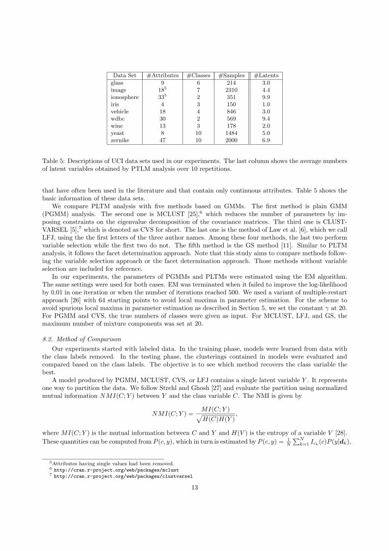
glass 9 6 214 3.0image 185 7 2310 4.4ionosphere 335 2 351 9.9iris 4 3 150 1.0vehicle 18 4 846 3.0wdbc 30 2 569 9.4wine 13 3 178 2.0yeast 8 10 1484 5.0zernike 47 10 2000 6.9

Table 5: Descriptions of UCI data sets used in our experiments. The last column shows the average numbersof latent variables obtained by PTLM analysis over 10 repetitions.

that have often been used in the literature and that contain only continuous attributes. Table 5 shows thebasic information of these data sets.

We compare PLTM analysis with five methods based on GMMs. The first method is plain GMM(PGMM) analysis. The second one is MCLUST [25],6 which reduces the number of parameters by im-posing constraints on the eigenvalue decomposition of the covariance matrices. The third one is CLUST-VARSEL [5],7 which is denoted as CVS for short. The last one is the method of Law et al. [6], which we callLFJ, using the the first letters of the three author names. Among these four methods, the last two performvariable selection while the first two do not. The fifth method is the GS method [11]. Similar to PLTManalysis, it follows the facet determination approach. Note that this study aims to compare methods follow-ing the variable selection approach or the facet determination approach. Those methods without variableselection are included for reference.

In our experiments, the parameters of PGMMs and PLTMs were estimated using the EM algorithm.The same settings were used for both cases. EM was terminated when it failed to improve the log-likelihoodby 0.01 in one iteration or when the number of iterations reached 500. We used a variant of multiple-restartapproach [26] with 64 starting points to avoid local maxima in parameter estimation. For the scheme toavoid spurious local maxima in parameter estimation as described in Section 5, we set the constant γ at 20.For PGMM and CVS, the true numbers of classes were given as input. For MCLUST, LFJ, and GS, themaximum number of mixture components was set at 20.

8.2. Method of Comparison

Our experiments started with labeled data. In the training phase, models were learned from data withthe class labels removed. In the testing phase, the clusterings contained in models were evaluated andcompared based on the class labels. The objective is to see which method recovers the class variable thebest.

A model produced by PGMM, MCLUST, CVS, or LFJ contains a single latent variable Y . It representsone way to partition the data. We follow Strehl and Ghosh [27] and evaluate the partition using normalizedmutual information NMI(C;Y ) between Y and the class variable C. The NMI is given by

NMI(C;Y ) =MI(C;Y )√H(C)H(Y )

,

where MI(C;Y ) is the mutual information between C and Y and H(V ) is the entropy of a variable V [28].

These quantities can be computed from P (c, y), which in turn is estimated by P (c, y) = 1N

∑Nk=1 Ick(c)P (y|dk),

5Attributes having single values had been removed.6 http://cran.r-project.org/web/packages/mclust7 http://cran.r-project.org/web/packages/clustvarsel

13

Facet Determination Variable Selection No Variable SelectionData Set PLTM GS CVS LFJ PGMM MCLUST

synthetic .85 (.00) .69 (.00) .34 (.00) .56 (.02) .56 (.00) .64 (.00)glass .43 (.03) .38 (.00) .29 (.00) .35 (.03) .28 (.03) .33 (.00)image .71 (.03) .65 (.00) .41 (.00) .51 (.03) .52 (.04) .66 (.00)vehicle .40 (.04) .31 (.00) .23 (.00) .27 (.01) .25 (.08) .36 (.00)wine .97 (.00) .83 (.00) .71 (.00) .70 (.19) .50 (.06) .69 (.00)zernike .50 (.02) .39 (.00) .33 (.00) .45 (.01) .44 (.03) .41 (.00)ionosphere .36 (.01) .26 (.00) .41 (.00) .13 (.07) .57 (.04) .32 (.00)iris .76 (.00) .74 (.00) .87 (.00) .68 (.02) .73 (.08) .76 (.00)wdbc .45 (.03) .36 (.00) .34 (.00) .41 (.02) .44 (.08) .68 (.00)yeast .18 (.00) .22 (.00) .04 (.00) .11 (.04) .16 (.01) .11 (.00)

Table 6: Clustering performances as measured by NMI. The averages and standard deviations over 10repetitions are reported. Best results are highlighted in bold. The first row categorizes the methods accordingto their approaches.

where d1, . . . ,dN are the samples in testing data, Ick(c) is an indicator function having value of 1 whenc = ck and 0 otherwise, and ck is the class label for the k-th sample.

A model resulting from PLTM analysis or the GS method contains a set Y of latent variables. Each ofthe latent variables represents a partition of the data. In practice, the user may find several of the partitionsinteresting and use them all in his work. In this section, however, we are talking about comparing differentclustering algorithms in terms of the ability to recover the original class partition. So, the user needs tochoose one of the partitions as the final result. The question becomes whether this analysis provides thepossibility for the user to recover the original class partition. Consequently, we assume that the user chooses,among all the partitions produced, the one closest to the class partition and we evaluate the performanceof PLTM analysis and the GS method using this quantity:

maxY ∈Y

NMI(C;Y ).

Note that NMI was used in our experiments due to the absence of a domain expert to evaluate theclustering results. In practice, class labels are not available when we cluster data. Hence, NMI cannot beused to select the appropriate partitions in the facet determination approach. A user needs to interpret theclusterings and find those interesting to her. It might also be possible to use clustering validity indices [29]for selection. Investigation into this possibility is left for future research.

8.3. Results

The results of our experiments are given in Table 6. In terms of NMI, PLTM had clearly superiorperformances over the two variable selection methods, CVS and LFJ. Specifically, it outperformed CVSon all but one data sets and LFJ on all data sets. PLTM also performed better than GS, the other facetdetermination method. It outperformed GS on all but one data. Besides, PLTM has clear advantages overPGMM and MCLUST, the two methods that do not do variable selection. PLTM outperformed PGMMon all but one data sets and outperformed MCLUST except for two data sets. On those data sets in ourexperiments, PLTM usually outperformed the other methods by large margins.

Note that multiple clusterings are produced by PLTMs and maximum NMI scores are used for compar-ison. It is therefore possible that not all of the clusterings produced by PLTM analysis have higher NMIscores than clusterings obtained by other methods, even if PLTM analysis has a higher maximum NMI score.Moreover, the clusterings produced by other methods may appear more interesting if the interest of userslies not in the class partitions. Nevertheless, our comparison assumes that users are only interested in theclass partitions. Indeed, this is an assumption taken implicitly when the class partitions are used for the

14

Y1Y2

Z1Z2

0.0

0.1

0.2

0.3

0.4

0.5

X1 X2 X3 X4 X5 X6 X7 X8 X9Features

NMI

(a) PLTM analysis

Y1Y2CVS

LFJGS1GS2

0.0

0.1

0.2

0.3

0.4

0.5

X1 X2 X3 X4 X5 X6 X7 X8 X9Features

NMI

(b) Variable selection methods and GS

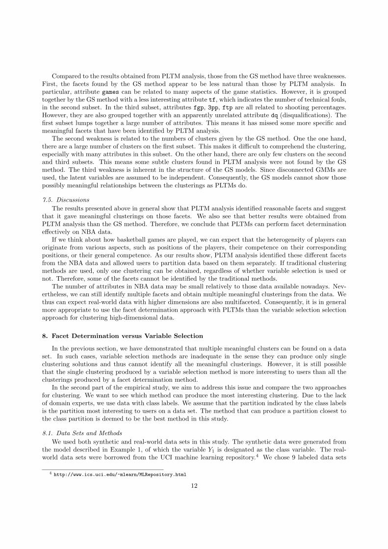
Figure 5: Feature curves of the partitions obtained by various methods and that of the original class partitionon synthetic data.

evaluation of clusterings. Based on this assumption, the experimental results indicate that PLTM analysisusually provides the best possibility for recovering the partitions of interest.

8.4. Explaining the Results

We next examine models produced by the various methods to gain insights about the superior perfor-mance of PLTM analysis. This also allows us to judge the facets identified by PLTM analysis.

8.4.1. Synthetic Data

Before examining models obtained from synthetic data, we first take a look at the data set itself. Thedata were sampled from the model shown in Figure 1b, with information about the two latent variables Y1and Y2 removed. Nonetheless, the latent variables represent two natural ways to partition the data. Tosee how the partitions are related to the attributes, we plot the NMI8 between the latent variables and theattributes in Figure 5a. We call the curve for a latent variable its feature curve. We see that Y1 is stronglycorrelated with X1–X3, but not with the other attributes. Hence it represents a partition based on thosethree attributes. Similarly, Y2 represents a partition of the data based on attributes X4–X9. So, we say thatthe data has two facets, one represented by X1–X3 and another by X4–X9. The designated class partitionY1 is a partition along the first facet.

The model produced by PLTM analysis has the same structure as the generative model. We name thetwo latent variables in the model Z1 and Z2 respectively. Their feature curves are also shown in Figure 5a.We see that the feature curves of Z1 and Z2 match those of Y1 and Y2 well. This indicates that PLTManalysis has successfully recovered the two facets of the data. It has also produced a partition of the dataalong each of the facets. If the user chooses the partition Z1 along the facet X1–X3 as the final result, thenthe original class partition is well recovered. This explains the good performance of PLTM (NMI=0.85).

The feature curves of the partitions obtained by LFJ and CVS are shown in Figure 5b. We see thatthe LFJ partition is not along any of the two natural facets of the data. Rather it is a partition based ona mixture of those two facets. Consequently, the performance of LFJ (NMI=0.56) is not as good as thatof PLTM. CVS did identify the facet represented by X4–X9, but it is not the facet of the designated classpartition. In other words, it picked the wrong facet. Consequently, the performance of CVS (NMI=0.34) isthe worst among all the methods considered. GS succeeded to identify two facets. However, the their feature

8To compute NMI(X;Y ) between a continuous variable X and a latent variable Y , we discretized X into 10 equal-widthbins, so that P (X,Y ) could be estimated as a discrete distribution.

15

classY1Y2Y3Y4

0.0

0.2

0.4

0.6

line.density.5

line.density.2

vedge.mean

vedge.sd

hedge.mean

hedge.sd

intensityrawred

rawblue

rawgreenexredexblue

exgreenvalue

saturationhu

e

centroid.row

centroid.col

Features

NMI

(a) PLTM analysis

classCVSLFJ

0.0

0.2

0.4

0.6

line.density.5

line.density.2

vedge.mean

vedge.sd

hedge.mean

hedge.sd

intensityrawred

rawblue

rawgreenexredexblue

exgreenvalue

saturationhu

e

centroid.row

centroid.col

Features

NMI

(b) Variable selection methods

classGS1GS2

0.0

0.2

0.4

0.6

line.density.5

line.density.2

vedge.mean

vedge.sd

hedge.mean

hedge.sd

intensityrawred

rawblue

rawgreenexredexblue

exgreenvalue

saturationhu

e

centroid.row

centroid.col

Features

NMI

(c) GS

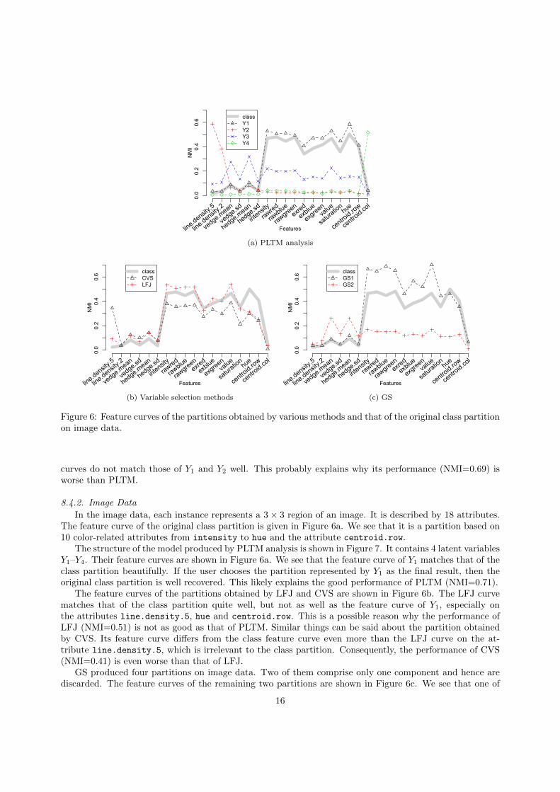
Figure 6: Feature curves of the partitions obtained by various methods and that of the original class partitionon image data.

curves do not match those of Y1 and Y2 well. This probably explains why its performance (NMI=0.69) isworse than PLTM.

8.4.2. Image Data

In the image data, each instance represents a 3× 3 region of an image. It is described by 18 attributes.The feature curve of the original class partition is given in Figure 6a. We see that it is a partition based on10 color-related attributes from intensity to hue and the attribute centroid.row.

The structure of the model produced by PLTM analysis is shown in Figure 7. It contains 4 latent variablesY1–Y4. Their feature curves are shown in Figure 6a. We see that the feature curve of Y1 matches that of theclass partition beautifully. If the user chooses the partition represented by Y1 as the final result, then theoriginal class partition is well recovered. This likely explains the good performance of PLTM (NMI=0.71).

The feature curves of the partitions obtained by LFJ and CVS are shown in Figure 6b. The LFJ curvematches that of the class partition quite well, but not as well as the feature curve of Y1, especially onthe attributes line.density.5, hue and centroid.row. This is a possible reason why the performance ofLFJ (NMI=0.51) is not as good as that of PLTM. Similar things can be said about the partition obtainedby CVS. Its feature curve differs from the class feature curve even more than the LFJ curve on the at-tribute line.density.5, which is irrelevant to the class partition. Consequently, the performance of CVS(NMI=0.41) is even worse than that of LFJ.

GS produced four partitions on image data. Two of them comprise only one component and hence arediscarded. The feature curves of the remaining two partitions are shown in Figure 6c. We see that one of

16

Figure 7: Structure of the PLTM learned from image data.

Figure 8: Structure of the PLTM learned from wine data.

them corresponds to the facet of the class partition, but does not match that well. This likely explains whythe performance of GS (NMI=0.65) is better than the other methods but is not as good as that of PLTM.

Two remarks are in order. First, the 10 color-related attributes semantically form a facet of the data.PLTM analysis has identified the facet in the pouch below Y1. Moreover, it obtained a partition based onnot only the color attributes, but also the attribute centroid.row, the vertical location of a region in animage. This is interesting. It is because centroid.row is closely related to the color facet. Intuitively, thevertical location of a region should correlate with the color of the region. For example, the color of the skyoccurs more frequently at the top of an image and that of grass more frequently at the bottom.

Second, the latent variable Y2 is strongly correlated with the two line density attributes. This is anotherfacet of the data that PLTM analysis has identified. PLTM analysis has also identified the edge-relatedfacet in the pouch node below Y3. However, it did not obtain a partition along the facet. The partitionrepresented by Y3 depends on not only the edge attributes but others as well. The two coordinate attributescentroid.row and centroid.col semantically form one facet. The facet has not been identified probablybecause the two attributes are not correlated.

8.4.3. Wine Data

The PLTM learned from wine data is shown in Figure 8. The model structure also appears to beinteresting. While we are not experts on wine, it seems natural to have Ash and Alcalinity of ash in onepouch as both are related to ash. Similarly, Flavanoids, Nonflavanoid phenols, and Total phenols arerelated to phenolic compounds. These compounds affect the color of wine, so it is reasonable to have them inone pouch along with the opacity attribute OD280/OD315. Moreover, both Magnesium and Malic acid playa role in the production of ATP (adenosine triphosphate), the most essential chemical in energy production.So, it is not a surprise to find them connected to a second latent variable.

17

Figure 9: Structure of the PLTM learned from wdbc data.

classY1Y1(2)

0.0

0.2

0.4

0.6

0.8

radius.w

radius.s

radius.m

perimeter.w

perimeter.s

perimeter.m

compactness.marea.warea.s

area.m

fractal_dim.w

concavity.w

concavity.m

concave_pts.w

concave_pts.m

compactness.w

symmetry.w

symmetry.m

smoothness.w

smoothness.m

concave_pts.s

concavity.s

compactness.s

fractal_dim.s

fractal_dim.m

smoothness.s

texture.w

texture.s

texture.m

symmetry.s

Features

NMI

Figure 10: Features curves of the partition Y1, obtained by PLTM, and that of the original class partitionon wdbc data. Y1(2) is obtained by setting the cardinality of Y1 to 2.

8.4.4. WDBC Data

After examining some positive cases for PLTM analysis, we now look at a data set that PLTM did notperform so well. Here we consider wdbc data. The data were obtained from 569 digitalized images of cellnuclei aspirated from breast masses. Each image corresponds to a data instance. It is labeled as eitherbenign or malignant. There are 10 computed features of the cell nuclei in the images. The attributes consistof the mean value (m), standard error (s), and worst value (w) for each of these features.

Figure 9 shows the structure of a PLTM learned from this data. We can see that this model identifiessome meaningful facets. The pouch below Y1 identifies a facet related to the size of nuclei. It mainly includesattributes related to area, perimeter, and radius. The second facet is identified by the pouch below Y2. Itis related to concavity and consists primarily of the mean and worst values of the two features related toconcavity. The third facet is identified by the pouch below Y3. It includes the mean and worst values ofsmoothness and symmetry. The facet appears to show whether the nuclei have regular shapes or not. Thepouch below Y9 identifies a facet primarily related to texture. This facet includes three texture-relatedattributes but also the attribute symmetry.s. The remaining attributes are mostly standard errors of somefeatures and may be considered as the amount of variation of the features. They are connected to the restof the model through Y4 and Y8.

Although the model appears to have a reasonable structure, it did not achieve a high NMI on this data(NMI=0.45). To have better understanding, we compare the feature curve of the class partition with that of

18

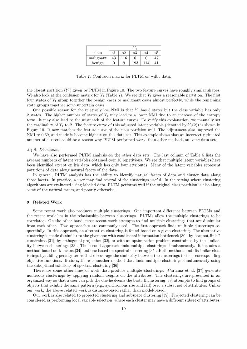
Y1class s1 s2 s3 s4 s5

malignant 43 116 6 0 47benign 0 9 193 114 41

Table 7: Confusion matrix for PLTM on wdbc data.

the closest partition (Y1) given by PLTM in Figure 10. The two feature curves have roughly similar shapes.We also look at the confusion matrix for Y1 (Table 7). We see that Y1 gives a reasonable partition. The firstfour states of Y1 group together the benign cases or malignant cases almost perfectly, while the remainingstate groups together some uncertain cases.

One possible reason for the relatively low NMI is that Y1 has 5 states but the class variable has only2 states. The higher number of states of Y1 may lead to a lower NMI due to an increase of the entropyterm. It may also lead to the mismatch of the feature curves. To verify this explanation, we manually setthe cardinality of Y1 to 2. The feature curve of this adjusted latent variable (denoted by Y1(2)) is shown inFigure 10. It now matches the feature curve of the class partition well. The adjustment also improved theNMI to 0.69, and made it become highest on this data set. This example shows that an incorrect estimatednumber of clusters could be a reason why PLTM performed worse than other methods on some data sets.

8.4.5. Discussions

We have also performed PLTM analysis on the other data sets. The last column of Table 5 lists theaverage numbers of latent variables obtained over 10 repetitions. We see that multiple latent variables havebeen identified except on iris data, which has only four attributes. Many of the latent variables representpartitions of data along natural facets of the data.

In general, PLTM analysis has the ability to identify natural facets of data and cluster data alongthose facets. In practice, a user may find several of the clusterings useful. In the setting where clusteringalgorithms are evaluated using labeled data, PLTM performs well if the original class partition is also alongsome of the natural facets, and poorly otherwise.

9. Related Work

Some recent work also produces multiple clusterings. One important difference between PLTMs andthe recent work lies in the relationship between clusterings. PLTMs allow the multiple clusterings to becorrelated. On the other hand, most recent work attempts to find multiple clusterings that are dissimilarfrom each other. Two approaches are commonly used. The first approach finds multiple clusterings se-quentially. In this approach, an alternative clustering is found based on a given clustering. The alternativeclustering is made dissimilar to the given one with conditional information bottleneck [30], by “cannot-links”constraints [31], by orthogonal projection [32], or with an optimization problem constrained by the similar-ity between clusterings [33]. The second approach finds multiple clusterings simultaneously. It includes amethod based on k-means [34] and one based on spectral clustering [35]. Both methods find dissimilar clus-terings by adding penalty terms that discourage the similarity between the clusterings to their correspondingobjective functions. Besides, there is another method that finds multiple clusterings simultaneously usingthe suboptimal solutions of spectral clustering [36].

There are some other lines of work that produce multiple clusterings. Caruana et al. [37] generatenumerous clusterings by applying random weights on the attributes. The clusterings are presented in anorganized way so that a user can pick the one he deems the best. Biclustering [38] attempts to find groups ofobjects that exhibit the same pattern (e.g., synchronous rise and fall) over a subset set of attributes. Unlikeour work, the above related work is distance-based rather than model-based.

Our work is also related to projected clustering and subspace clustering [39]. Projected clustering can beconsidered as performing local variable selection, where each cluster may have a different subset of attributes.

19

It produces only a single clustering as variable selection methods do. Subspace clustering considers denseregions as clusters and tries to identify all clusters in all subspaces. However, it does not partition dataalong those identified subspaces. In other words, some data points may not be assigned to any cluster in anidentified subspace. This is different from the facet determination approach, in which data are partitionedalong every identified facet.

In terms of model definition, the AutoClass models [40] and the MULTIMIX models [41] are some mixturemodels that are related to our work. The manifest variables in those models have multivariate Gaussiandistributions and are similar to the pouch nodes in PLTMs. However, those models do not allow multiplelatent variables.

10. Concluding Remarks

In this paper, we have proposed PLTMs as a generalization of GMMs and empirically compared PLTManalysis with several GMM-based methods. Real-world high-dimensional data are usually multifaceted andinteresting clusterings in such data often are relevant only to subsets of attributes. One way to identifysuch clusterings is to perform variable selection. Another way is to perform facet determination by PLTManalysis. Our work has shown that PLTM analysis is often more effective than the first approach.

One drawback of PLTM analysis is that the training is slow. For example, one run of PLTM analysistook around 5 hours on data sets of moderate size (e.g., image, ionosphere, and wdbc data) and around 2.5days on the largest data set (zernike data) in our experiments. This prohibits the use of PLTM analysis ondata with very high dimensions. For example, PLTM analysis is currently infeasible for data with hundredsor thousands of attributes, such as those for text mining and gene expression analysis. On the other hand,even though NBA data has only 18 attributes, our experiment demonstrated that PLTM analysis on thatdata could still identify multiple meaningful facets. This suggests that PLTM analysis can be useful for datasets that have tens of attributes. One possibly fruitful application of PLTMs is for analyzing survey data.Those data usually have only tens of attributes and are likely to be multifaceted.

A future direction of this work is to speed up the learning of PLTMs, so that PLTM analysis can beapplied in more areas. This can possibly be done by parallelization. Recently, some structural learningmethods for LTMs have been proposed to follow a variable clustering approach [13, 42, 43] or a constraint-based approach [44, 45]. The learning of PLTMs can also possibly be sped up by following those approaches.

We have made available online the data sets and the Java implementation of the algorithm used in theexperiments. They can be found on http://www.cse.ust.hk/faculty/lzhang/ltm/index.htm.

Acknowledgements

Research on this work was supported by National Basic Research Program of China (aka the 973 Pro-gram) under project No. 2011CB505101 and HKUST Fok Ying Tung Graduate School.

Appendix A. Inference Algorithm

Consider a PLTM M with manifest variables X and latent variables Y . Recall that inference on Mrefers to the computation of the posterior probability P (q|e) of some variables of interest, Q ⊆X ∪Y , afterobserving values e of evidence variables E ⊆X. To perform inference, M has to be converted into a cliquetree T . A propagation scheme for message passing can then be carried out on T .

Construction of clique trees is simple due to the tree structure of PLTMs. To construct T , a clique C isadded to T for each edge in M , such that C = V ∪{Π(V )} contains the variable(s) V of the child node andvariable Π(V ) of its parent node. Two cliques are then connected in T if they share any common variable.The resulting clique tree contains two types of cliques. The first type are discrete cliques. Each one containstwo discrete variables. The second type are mixed cliques. Each one contains the continuous variables of apouch node and the discrete variable of its parent node. Observe that in a PLTM all the internal nodes are

20

Algorithm 1 Inference Algorithm

1: procedure Propagate(M, T ,E, e)2: Initialize ψ(C) for every clique C3: Incorporate evidence to the potentials4: Choose an arbitrary clique in T as CP

5: for all C ∈ Ne(CP ) do6: CollectMessage(CP , C)7: end for8: for all C ∈ Ne(CP ) do9: DistributeMessage(CP , C)

10: end for11: Normalize ψ(C) for every clique C12: end procedure

13: procedure CollectMessage(C,C′)14: for all C′′ ∈ Ne(C′)\{C} do15: CollectMessage(C′, C′′)16: end for17: SendMessage(C′, C)18: end procedure

19: procedure DistributeMessage(C,C′)20: SendMessage(C,C′)21: for all C′′ ∈ Ne(C′)\{C} do22: DistributeMessage(C′, C′′)23: end for24: end procedure

25: procedure SendMessage(C,C′)26: φ← RetrieveFactor(C ∩ C′)27: φ′ ←

∑C\C′ ψ(C)

28: SaveFactor(C ∩ C′, φ′)29: ψ(C′)← ψ(C′)× φ′/φ30: end procedure

31: procedure RetrieveFactor(S)32: If SaveFactor(S, φ) has been called, return φ;

otherwise, return 1.33: end procedure

// Ne(C) denotes the neighbors of C

discrete and only leaf nodes are continuous. Consequently, the clique tree can be considered as a clique treeconsisted of all discrete cliques, with some mixed cliques attaching to it on the boundary.

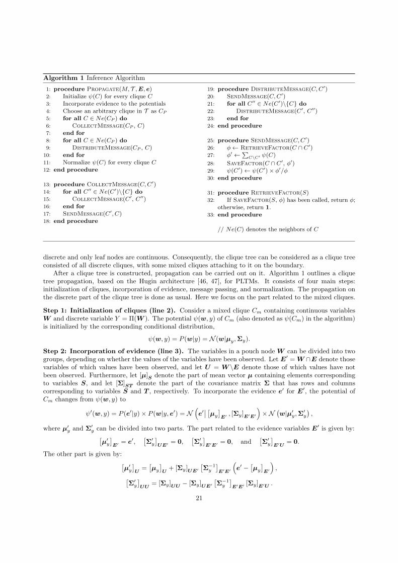
After a clique tree is constructed, propagation can be carried out on it. Algorithm 1 outlines a cliquetree propagation, based on the Hugin architecture [46, 47], for PLTMs. It consists of four main steps:initialization of cliques, incorporation of evidence, message passing, and normalization. The propagation onthe discrete part of the clique tree is done as usual. Here we focus on the part related to the mixed cliques.

Step 1: Initialization of cliques (line 2). Consider a mixed clique Cm containing continuous variablesW and discrete variable Y = Π(W ). The potential ψ(w, y) of Cm (also denoted as ψ(Cm) in the algorithm)is initialized by the corresponding conditional distribution,

ψ(w, y) = P (w|y) = N (w|µy,Σy).

Step 2: Incorporation of evidence (line 3). The variables in a pouch node W can be divided into twogroups, depending on whether the values of the variables have been observed. Let E′ = W ∩E denote thosevariables of which values have been observed, and let U = W \E denote those of which values have notbeen observed. Furthermore, let [µ]S denote the part of mean vector µ containing elements correspondingto variables S, and let [Σ]ST denote the part of the covariance matrix Σ that has rows and columnscorresponding to variables S and T , respectively. To incorporate the evidence e′ for E′, the potential ofCm changes from ψ(w, y) to

ψ′(w, y) = P (e′|y)× P (w|y, e′) = N(e′∣∣ [µy]E′ , [Σy]E′E′

)×N

(w|µ′y,Σ

′y

),

where µ′y and Σ′y can be divided into two parts. The part related to the evidence variables E′ is given by:[µ′y]E′ = e′,

[Σ′y]UE′ = 0,

[Σ′y]E′E′ = 0, and

[Σ′y]E′U

= 0.

The other part is given by:[µ′y]U

=[µy]U

+ [Σy]UE′

[Σ−1y

]E′E′

(e′ −

[µy]E′

),[

Σ′y]UU

= [Σy]UU − [Σy]UE′

[Σ−1y

]E′E′ [Σy]E′U .

21

Step 3: Message passing (lines 5–10). In this step, Cm involves two operations, marginalization andcombination. Marginalization of ψ′(w, y) over W is required for sending out a message from Cm (line 27).It results in a potential ψ′(y), involving only the discrete variable y, as given by:

ψ′(y) = P (e′|y) = N(e′∣∣ [µy]E′ , [Σy]E′E′

).

Combination is required for sending a message to Cm (line 29). The combination of the potential ψ′(w, y)with a discrete potential φ(y) is given by ψ′′(w, y) = ψ′(w, y)× φ(y). When the message passing completes(line 10), ψ′′(w, y) represents the distribution

ψ′′(w, y) = P (y, e)× P (w|y, e′) = P (y, e)×N(w|µ′y,Σ

′y

).

Step 4: Normalization (line 11). In this step, a potential changes from ψ′′(w, y) to

ψ′′′(w, y) = P (y|e)× P (w|y, e′) = P (y|e)×N(w|µ′y,Σ

′y

).

For implementation, the potential of a mixed clique is usually represented by two types of data structures:one for the discrete distribution and one for the conditional Gaussian distribution. More details for thegeneral clique tree propagation can be found in [46, 21, 48].

Appendix B. Search Algorithm

Some issues for the search algorithm of latent tree models are studied in [49, 14]. These issues also affectPLTMs. In this section, we discuss how these issues are addressed for PTLMs. We summarize the entiresearch algorithm for PLTMs at the end of this section.

Appendix B.1. Three Search Phases

In every search step, a search operator generates all possible candidate models for consideration. Let land b be the numbers of latent nodes and pouch nodes, respectively, and n = l+ b be total number of nodes.Let p, q, and r be the maximum number of variables in a pouch node, the maximum number of siblingpouch nodes, and the maximum number of neighbors of a latent node, respectively. The numbers of possiblecandidate models that NI, ND, SI, SD, NR, PO, and UP can generate are O(lr(r − 1)/2), O(lr), O(l),O(l), O(nl), O(lq(q − 1)/2), and O(bp), respectively. If we consider all seven operators in each search step,many candidate models are generated but only one of them is chosen for the next step. Those suboptimalmodels are discarded and are not used for the next step. Therefore, in some sense, much time are wastedfor considering the suboptimal models.

A more efficient way is to consider fewer candidate models in each search step. This can be achieved byconsidering only a subset of search operators at a time. The search operators can be naturally partitionedinto three categories. SI, NI, and PO belong to the expansion category, since all of them can create candidatemodels that are more complex than the current one. SD, ND, and UP, which simplify a model, belong tothe simplification category. NR does not change the complexity considerably. It belongs to the adjustmentcategory. We therefore perform search in three phases, each of which considers only operators in onecategory. The best model found in each phase is used to seed the next phase, and the search repeats thesethree phases until all three phases cannot find a better model. This search is called EAST, since it doesExpansion, Adjustment, and Simplification until Termination.

Appendix B.2. Efficient Model Evaluation

Suppose m is the current model after a number of search steps. A candidate model m′ can be obtainedfrom m by applying a search operator. Very often, the search operator modifies only a small part of m, sothat m and m′ share a large number of parameters. For example, consider the model m2, that is obtainedfrom model m1 using the PO operator, as shown in Figure 3. m1 and m2 shares many parameters such asP (x1, x2|y2), P (y2|y1), P (y3|y1), P (x6|y3), etc. On the other hand, some parameters are not shared by m

22

and m′. In this example, parameters P (x4|y3) and P (x5|y3) are specific to m1, while parameter P (x4, x5|y3)is specific to m2. We can divide the parameters of m′ into two groups and write the parameters θ′ of m′ as(θ′1,θ

′2). θ′1 consists of parameters shared with m, while θ′2 consists of parameters specific to m′. Similarly,

we write the parameters of m as θ = (θ1,θ2).Suppose we have computed the MLE θ∗ = (θ∗1,θ

∗2) of the parameters of m. θ∗1 can be used as estimates

for the shared parameters of m′. Consequently, we can obtain a likelihood function P (D|m′,θ∗1,θ′2) that

depends on only the unshared parameters θ′2. This function is referred to as restricted likelihood functionof m′. As previously described, we use the BIC score to evaluate a candidate model. This requires themaximum log-likelihood (ML) of m′. Instead of computing the ML over all parameters of m′, we mayapproximate it by maximizing the restricted log-likelihood over only the subset of parameters θ′2. Thisresults in an approximate score given by

BICRL(m′|D) = maxθ′2

logP (D|m′,θ∗1,θ′2)− d(m′)

2logN.

The advantage of using BICRL is that it allows a more efficient implementation of EM. This is due totwo reasons. First, it involves a maximization of fewer parameters in the M-step. This also means fewercomputations in the E-step, since only distributions relevant to θ′2 need to be computed. Second, the E-stepcan exploit the fixed parameters θ∗1 to allow sharing of computation among all iterations of EM. Specifically,the E-step requires inference on a PLTM, which in turn requires passing messages in the clique tree. As theparameters θ∗1 do not change in these iterations, the messages that depend on only these parameters remainthe same in all iterations. Therefore, some messages can be cached for each data case and can be shared forthe inference used in subsequent E-steps.

In our implementation, both BIC and BICRL are used to evaluate models, but at different situations.The approximation BICRL is used for quickly evaluating candidate models generated by the same searchoperator, while the real BIC is used for accurately evaluating the candidate model with the highest BICRLfor each of the search operators. This improves the speed for the evaluation of models within search operators,but maintains the accuracy for the evaluation of models across search operators.

Appendix B.3. Operation Granularity

Operation granularity refers to the phenomenon where some search operators might increase the com-plexity of the current model much more than other search operators. If we use BIC to evaluate candidatemodels given by the search operators, those having a much larger increase in complexity are usually pre-ferred. This might lead to local maxima. Therefore, we adopt a simple and effective strategy called thecost-effectiveness principle for evaluating the candidate models. Let m be the current model and m′ be acandidate model. Define the improvement ratio of m′ over m given data D to be

IR(m′,m|D) =BIC(m′|D)−BIC(m|D)

d(m′)− d(m).

It is the increase in model score per unit increase in model complexity. The cost-effectiveness principlestipulates that one chooses, among a list of candidate models, the one with the highest improvement ratio.

The principle is applied only on candidate models generated by the SI, NI, and PO operators. In otherwords, it is used only during the expansion phase. The principle is not applied for other operators sincethey do not or do not necessarily increase model complexity.

Appendix B.4. PLTM-EAST

The entire search algorithm for PLTMs is named PLTM-EAST. It is outlined in Algorithm 2. Thesearch process starts with the initial model m(0) described in Section 6. The procedure PLTM-EAST usesm(0) as the first current model. It then repeatedly tries to improve the current model in the three differentphases.

In procedure Expand, the improvement ratio IR is used to pick the best models among the candidatemodels generated by SI, NI, and PO. It stops when the best candidate model fails to improve over the

23

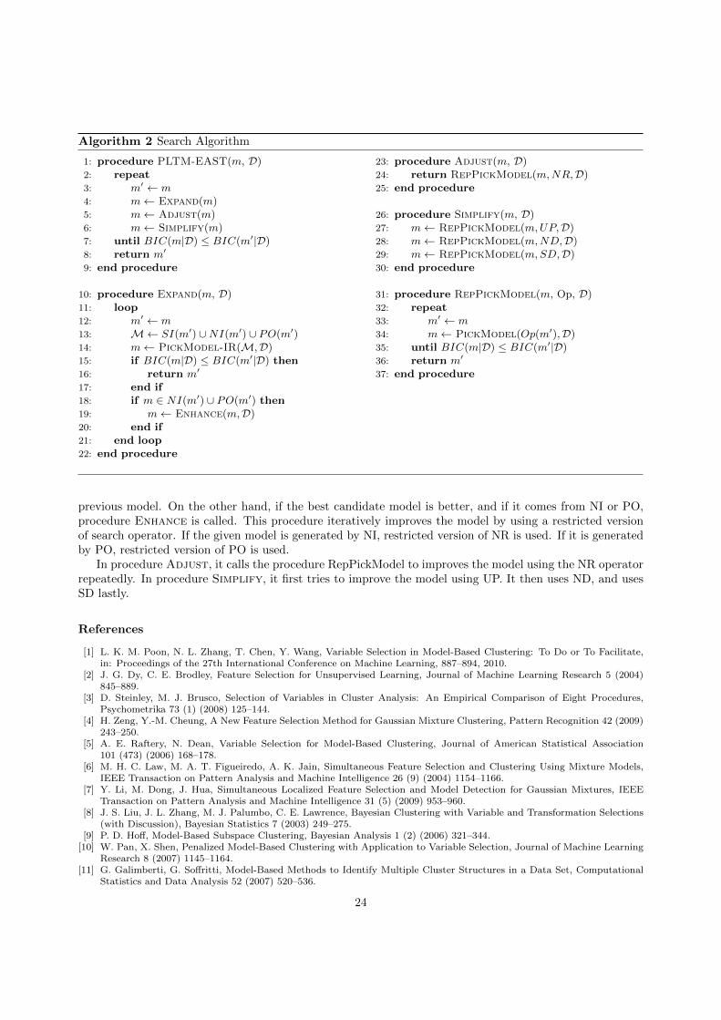
Algorithm 2 Search Algorithm

1: procedure PLTM-EAST(m, D)2: repeat3: m′ ← m4: m← Expand(m)5: m← Adjust(m)6: m← Simplify(m)7: until BIC(m|D) ≤ BIC(m′|D)8: return m′

9: end procedure

10: procedure Expand(m, D)11: loop12: m′ ← m13: M← SI(m′) ∪NI(m′) ∪ PO(m′)14: m← PickModel-IR(M,D)15: if BIC(m|D) ≤ BIC(m′|D) then16: return m′

17: end if18: if m ∈ NI(m′) ∪ PO(m′) then19: m← Enhance(m,D)20: end if21: end loop22: end procedure

23: procedure Adjust(m, D)24: return RepPickModel(m,NR,D)25: end procedure

26: procedure Simplify(m, D)27: m← RepPickModel(m,UP,D)28: m← RepPickModel(m,ND,D)29: m← RepPickModel(m,SD,D)30: end procedure

31: procedure RepPickModel(m, Op, D)32: repeat33: m′ ← m34: m← PickModel(Op(m′),D)35: until BIC(m|D) ≤ BIC(m′|D)36: return m′

37: end procedure

previous model. On the other hand, if the best candidate model is better, and if it comes from NI or PO,procedure Enhance is called. This procedure iteratively improves the model by using a restricted versionof search operator. If the given model is generated by NI, restricted version of NR is used. If it is generatedby PO, restricted version of PO is used.

In procedure Adjust, it calls the procedure RepPickModel to improves the model using the NR operatorrepeatedly. In procedure Simplify, it first tries to improve the model using UP. It then uses ND, and usesSD lastly.

References

[1] L. K. M. Poon, N. L. Zhang, T. Chen, Y. Wang, Variable Selection in Model-Based Clustering: To Do or To Facilitate,in: Proceedings of the 27th International Conference on Machine Learning, 887–894, 2010.

[2] J. G. Dy, C. E. Brodley, Feature Selection for Unsupervised Learning, Journal of Machine Learning Research 5 (2004)845–889.

[3] D. Steinley, M. J. Brusco, Selection of Variables in Cluster Analysis: An Empirical Comparison of Eight Procedures,Psychometrika 73 (1) (2008) 125–144.

[4] H. Zeng, Y.-M. Cheung, A New Feature Selection Method for Gaussian Mixture Clustering, Pattern Recognition 42 (2009)243–250.

[5] A. E. Raftery, N. Dean, Variable Selection for Model-Based Clustering, Journal of American Statistical Association101 (473) (2006) 168–178.

[6] M. H. C. Law, M. A. T. Figueiredo, A. K. Jain, Simultaneous Feature Selection and Clustering Using Mixture Models,IEEE Transaction on Pattern Analysis and Machine Intelligence 26 (9) (2004) 1154–1166.

[7] Y. Li, M. Dong, J. Hua, Simultaneous Localized Feature Selection and Model Detection for Gaussian Mixtures, IEEETransaction on Pattern Analysis and Machine Intelligence 31 (5) (2009) 953–960.

[8] J. S. Liu, J. L. Zhang, M. J. Palumbo, C. E. Lawrence, Bayesian Clustering with Variable and Transformation Selections(with Discussion), Bayesian Statistics 7 (2003) 249–275.

[9] P. D. Hoff, Model-Based Subspace Clustering, Bayesian Analysis 1 (2) (2006) 321–344.[10] W. Pan, X. Shen, Penalized Model-Based Clustering with Application to Variable Selection, Journal of Machine Learning

Research 8 (2007) 1145–1164.[11] G. Galimberti, G. Soffritti, Model-Based Methods to Identify Multiple Cluster Structures in a Data Set, Computational

Statistics and Data Analysis 52 (2007) 520–536.

24

[12] N. L. Zhang, Hierarchical Latent Class Models for Cluster Analysis, Journal of Machine Learning Research 5 (2004)697–723.

[13] Y. Wang, N. L. Zhang, T. Chen, Latent Tree Models and Approximate Inference in Bayesian Networks, Journal of ArtificialIntelligence Research 32 (2008) 879–900.

[14] T. Chen, N. L. Zhang, T. Liu, K. M. Poon, Y. Wang, Model-Based Multidimensional Clustering of Categorical Data,Artificial Intelligence 176 (2012) 2246–2269.

[15] G. J. McLachlan, D. Peel, Finite Mixture Models, Wiley, New York, 2000.[16] C. Fraley, A. E. Raftery, Model-Based Clustering, Discriminant Analysis, and Density Estimation, Journal of American

Statistical Association 97 (458) (2002) 611–631.[17] A. P. Dempster, N. M. Laird, D. B. Rubin, Maximum Likelihood from Incomplete Data Via the EM Algorithm, Journal

of the Royal Statistical Society. Series B (Methodological) 39 (1) (1977) 1–38.[18] J. R. S. Fonseca, M. G. M. S. Cardoso, Mixture-Model Cluster Analysis Using Information Theoretical Criteria, Intelligent

Data Analysis 11 (2007) 155–173.[19] J. Pearl, Probabilistic Reasoning in Intelligent Systems: Networks of Plausible Inference, Morgan Kaufmann Publishers,

San Mateo, California, 1988.[20] D. Geiger, D. Heckerman, Learning Gaussian Networks, Tech. Rep. MSR-TR-94-10, Microsoft Research, 1994.[21] S. L. Lauritzen, F. Jensen, Stable Local Computation with conditional Gaussian Distributions, Statistics and Computing

11 (2001) 191–203.[22] S. Ingrassia, A Likelihood-Based Constrained Algorithm for Multivariate Normal Mixture Models, Statistical Methods

and Applications 13 (2) (2004) 151–166.[23] G. Schwarz, Estimating the Dimension of a Model, The Annals of Statistics 6 (2) (1978) 461–464.[24] N. L. Zhang, T. Kocka, Efficient Learning of Hierarchical Latent Class Models, in: Proceedings of the 16th IEEE Inter-

national Conference on Tools with Artificial Intelligence, 585–593, 2004.[25] C. Fraley, A. E. Raftery, MCLUST Version 3 for R: Normal Mixture Modeling and Model-Based Clustering, Tech. Rep.

504, Department of Statistics, University of Washington, (revised 2009), 2006.[26] D. M. Chickering, D. Heckerman, Efficient Approximations for the Marginal Likelihood of Bayesian Networks with Hidden

Variables, Machine learning 29 (1997) 181–212.[27] A. Strehl, J. Ghosh, Cluster Ensembles — A Knowledge Reuse Framework for Combining Multiple Partitions, Journal of

Machine Learning Research 3 (2002) 583–617.[28] T. M. Cover, J. A. Thomas, Elements of Information Theory, Wiley, 2nd edn., 2006.[29] M. Halkidi, Y. Batistakis, M. Vazirgiannis, On Clustering Validation Techniques, Journal of Intelligent Informaiton Sys-

tems 17 (2/3) (2001) 107–145.[30] D. Gondek, T. Hofmann, Non-Redundant Data Clustering, in: Proceedings of the Fourth IEEE International Conference

on Data Mining, 75–82, 2004.[31] E. Bae, J. Bailey, COALA: A Novel Approach for the Extraction of an Alternative Clustering of High Quality and High

Dissimilarity, in: Proceedings of the Sixth IEEE International Conference on Data Mining, 53–62, 2006.[32] Y. Cui, X. Z. Fern, J. G. Dy, Non-Reduntant Multi-View Clustering Via Orthogonalization, in: Proceedings of the Seventh

IEEE International Conferene on Data Mining, 133–142, 2007.[33] Z. Qi, I. Davidson, A Principled and Flexible Framework for Finding Alternative Clusterings, in: Proceedings of the 15th

ACM SIGKDD International Conference on Knowledge Discovery and Data Mining, 717–726, 2009.[34] P. Jain, R. Meka, I. S. Dhillon, Simultaneous Unsupervised Learning of Disparate Clusterings, in: Proceedings of the

Seventh SIAM International Converence on Data Mining, 858–869, 2008.[35] D. Niu, J. G. Dy, M. I. Jordan, Multiple Non-Redundant Spectral Clustering Views, in: Proceedings of the 27th Interna-

tional Conference on Machine Learning, 831–838, 2010.[36] S. Dasgupta, V. Ng, Mining Clustering Dimensions, in: Proceedings of the 27th International Conference on Machine

Learning, 263–270, 2010.[37] R. Caruana, M. Elhawary, N. Nguyen, C. Smith, Meta Clustering, in: Proceedings of the Sixth International Conference

on Data Mining, 107–118, 2006.[38] S. C. Madeira, A. L. Oliveria, Biclustering Algorithms for Biological Data Analysis: A Survey, IEEE Transactions on

Computational Biology and Bioinformatics 1 (1) (2004) 24–45.[39] H.-P. Kriegel, P. Kroger, A. Zimek, Clustering High Dimensional Data: A Survey on Subspace Clustering, Pattern-Based

Clustering, and Correlation Clustering, ACM Transactions on Knowledge Discovery from Data 3 (1) (2009) 1–58.[40] P. Cheeseman, J. Stutz, Bayesian Classification (AutoClass): Theory and Results, in: Advances in Knowledge Discovery

and Data Mining, AAAI Press, 153–180, 1996.[41] L. Hunt, M. Jorgensen, Mixture Model Clustering Using the MULTIMIX Program, Australian & New Zealand Journal of

Statistics 41 (2) (1999) 154–171.[42] Y. Wang, Latent Tree Models for Multivarite Density Estimation: Algorithms and Applications, Ph.D. thesis, Department

of Computer Science and Engineering, The Hong Kong University of Science and Technology, 2009.[43] S. Harmeling, C. K. I. Williams, Greedy Learning of Binary Latent Trees, IEEE Transaction on Pattern Analysis and

Machine Intelligence 33 (6) (2011) 1087–1097.[44] M. J. Choi, V. Y. F. Tan, A. Anandkumar, A. S. Willsky, Learning Latent Tree Graphical Models, Journal of Machine

Learning Research 12 (2011) 1771–1812.[45] A. Anandkumar, K. Chaudhuri, D. Hsu, S. M. Kakade, L. Song, T. Zhang, Spectral Methods for Learning Multivariate

Latent Tree Structure, in: Advances in Neural Information Processing Systems 24, 2025–2033, 2012.[46] R. G. Cowell, A. P. Dawid, S. L. Lauritzen, D. J. Spiegelhalter, Probabilistic Networks and Expert Systems, Springer,

25

1999.[47] A. Darwiche, Modeling and Reasoning with Bayesian Networks, Cambridge University Press, 2009.[48] R. G. Cowell, Local Propagation in Conditional Gaussian Bayesian Networks, Journal of Machine Learning Research 6

(2005) 1517–1550.[49] T. Chen, N. L. Zhang, Y. Wang, Efficient Model Evaluation in the Search-Based Approach to Latent Structure Discovery,

in: Proceedings of the Fourth European Workshop on Probabilistic Graphical Models, 57–64, 2008.

26