Modal dynamics of structures with bladed isotropic rotors ...
26
Wind Energ. Sci., 1, 271–296, 2016 www.wind-energ-sci.net/1/271/2016/ doi:10.5194/wes-1-271-2016 © Author(s) 2016. CC Attribution 3.0 License. Modal dynamics of structures with bladed isotropic rotors and its complexity for two-bladed rotors Morten Hartvig Hansen Dept. of Wind Energy, Technical University of Denmark, Frederiksborgvej 399, 4000 Roskilde, Denmark Correspondence to: Morten H. Hansen ([email protected]) Received: 2 August 2016 – Published in Wind Energ. Sci. Discuss.: 23 August 2016 Accepted: 7 November 2016 – Published: 30 November 2016 Abstract. The modal dynamics of structures with bladed isotropic rotors is analyzed using Hill’s method. First, analytical derivation of the periodic system matrix shows that isotropic rotors with more than two blades can be represented by an exact Fourier series with 3/rev (three per rotor revolution) as the highest order. For two-bladed rotors, the inverse mass matrix has an infinite Fourier series with harmonic components of decreasing norm; thus, the system matrix can be approximated by a truncated Fourier series of predictable accuracy. Second, a novel method for automatically identifying the principal solutions of Hill’s eigenvalue problem is introduced. The corresponding periodic eigenvectors can be used to compute symmetric and antisymmetric components of the two-bladed rotor motion, as well as the additional forward and backward whirling components for rotors with more than two blades. To illustrate the use of these generic methods, a simple wind turbine model is set up with three degrees of freedom for each blade and seven degrees of freedom for the nacelle and drivetrain. First, the model parameters are tuned such that the low-order modal dynamics of a three-bladed 10 MW turbine from previous studies is recaptured. Second, one blade is removed, leading to larger and higher harmonic terms in the system matrix. These harmonic terms lead to modal couplings for the two-bladed turbine that do not exist for the three-bladed turbine. A single mode of a two-bladed turbine will also have several resonance frequencies in both the ground-fixed and rotating frames of reference, which complicates the interpretation of simulated or measured turbine responses. 1 Introduction A fundamental understanding of the modal dynamics of structures with bladed rotors is relevant for the design and analysis of wind turbines, helicopters, and other rotating ma- chinery because their vibrational responses are composed of their structural modes. It is important to understand how these modes are excited by resonances or aeroelastic instabil- ities, i.e., at which frequencies and where on the structure or rotor the individual modes can be excited. Such knowledge is necessary not only for the interpretation of design simula- tions but also for the understanding of real measurements. The modal dynamics of three-bladed turbines is well un- derstood, also including the interaction with aerodynamic forces and a controller. For isotropic rotors, the Coleman transformation (Coleman and Feingold, 1958) is often used to transform the periodic system into a time-invariant sys- tem and then solving the associated eigenvalue problem with the blade motion described by the multi-blade coordinates (Hansen, 2003, 2004, 2007; van Engelen and Braam, 2004; Riziotis et al., 2008; Bir, 2008; Skjoldan and Hansen, 2009; Bergami and Hansen, 2016). The turbine modes may ei- ther be dominated by vibrations of the rotor support struc- ture and drivetrain, e.g., tower bending and shaft torsion modes, or by blade vibrations which herein are called the ro- tor modes. The rotor modes of the three-bladed isotropic ro- tor consist of a symmetric mode and two whirling modes for each blade mode (edgewise/flapwise bending and torsion). In the whirling modes, the order of blade vibration describes a backward (regressive) and a forward (progressive) whirling direction relative to the rotor rotation. Due to the anisotropy of the rotor support, the rotor modes are not “pure”, meaning that, for example, a backward whirling mode will also con- Published by Copernicus Publications on behalf of the European Academy of Wind Energy e.V.
Transcript of Modal dynamics of structures with bladed isotropic rotors ...

Wind Energ. Sci., 1, 271–296, 2016www.wind-energ-sci.net/1/271/2016/doi:10.5194/wes-1-271-2016© Author(s) 2016. CC Attribution 3.0 License.
Modal dynamics of structures with bladed isotropicrotors and its complexity for two-bladed rotors
Morten Hartvig HansenDept. of Wind Energy, Technical University of Denmark, Frederiksborgvej 399, 4000 Roskilde, Denmark
Correspondence to: Morten H. Hansen ([email protected])
Received: 2 August 2016 – Published in Wind Energ. Sci. Discuss.: 23 August 2016Accepted: 7 November 2016 – Published: 30 November 2016
Abstract. The modal dynamics of structures with bladed isotropic rotors is analyzed using Hill’s method. First,analytical derivation of the periodic system matrix shows that isotropic rotors with more than two blades can berepresented by an exact Fourier series with 3/rev (three per rotor revolution) as the highest order. For two-bladedrotors, the inverse mass matrix has an infinite Fourier series with harmonic components of decreasing norm;thus, the system matrix can be approximated by a truncated Fourier series of predictable accuracy. Second, anovel method for automatically identifying the principal solutions of Hill’s eigenvalue problem is introduced.The corresponding periodic eigenvectors can be used to compute symmetric and antisymmetric components ofthe two-bladed rotor motion, as well as the additional forward and backward whirling components for rotorswith more than two blades. To illustrate the use of these generic methods, a simple wind turbine model is setup with three degrees of freedom for each blade and seven degrees of freedom for the nacelle and drivetrain.First, the model parameters are tuned such that the low-order modal dynamics of a three-bladed 10 MW turbinefrom previous studies is recaptured. Second, one blade is removed, leading to larger and higher harmonic termsin the system matrix. These harmonic terms lead to modal couplings for the two-bladed turbine that do not existfor the three-bladed turbine. A single mode of a two-bladed turbine will also have several resonance frequenciesin both the ground-fixed and rotating frames of reference, which complicates the interpretation of simulated ormeasured turbine responses.
1 Introduction
A fundamental understanding of the modal dynamics ofstructures with bladed rotors is relevant for the design andanalysis of wind turbines, helicopters, and other rotating ma-chinery because their vibrational responses are composedof their structural modes. It is important to understand howthese modes are excited by resonances or aeroelastic instabil-ities, i.e., at which frequencies and where on the structure orrotor the individual modes can be excited. Such knowledgeis necessary not only for the interpretation of design simula-tions but also for the understanding of real measurements.
The modal dynamics of three-bladed turbines is well un-derstood, also including the interaction with aerodynamicforces and a controller. For isotropic rotors, the Colemantransformation (Coleman and Feingold, 1958) is often usedto transform the periodic system into a time-invariant sys-
tem and then solving the associated eigenvalue problem withthe blade motion described by the multi-blade coordinates(Hansen, 2003, 2004, 2007; van Engelen and Braam, 2004;Riziotis et al., 2008; Bir, 2008; Skjoldan and Hansen, 2009;Bergami and Hansen, 2016). The turbine modes may ei-ther be dominated by vibrations of the rotor support struc-ture and drivetrain, e.g., tower bending and shaft torsionmodes, or by blade vibrations which herein are called the ro-tor modes. The rotor modes of the three-bladed isotropic ro-tor consist of a symmetric mode and two whirling modes foreach blade mode (edgewise/flapwise bending and torsion). Inthe whirling modes, the order of blade vibration describes abackward (regressive) and a forward (progressive) whirlingdirection relative to the rotor rotation. Due to the anisotropyof the rotor support, the rotor modes are not “pure”, meaningthat, for example, a backward whirling mode will also con-
Published by Copernicus Publications on behalf of the European Academy of Wind Energy e.V.

272 M. H. Hansen: Modal dynamics of structures with bladed isotropic rotors
tain symmetric and forward whirling components when ob-served from the rotating blade frame of reference. The modalfrequency obtained from the eigenvalue problem describesthe frequency observed from the ground-fixed frame of ref-erence in which the multi-blade coordinates describes the ro-tor motion. In the rotating blade frame, the symmetric rotorresponse will be observable at the same frequency but thebackward and forward whirling components of a rotor modewill be shifted by +1/rev and −1/rev, respectively. Since arotor mode is not pure, its response may therefore be observ-able at three different frequencies in a signal measured on theblade (Hansen, 2003, 2007).
For anisotropic three-bladed rotors, Floquet theory orHill’s method is needed to obtain an eigenvalue problemwhich leads to the periodic eigenvectors of the principaleigenvalue solutions (Skjoldan and Hansen, 2009; Skjoldan,2009; Skjoldan and Hansen, 2009; Bottasso and Cacciola,2015). To handle the frequency indeterminacy of the peri-odic eigenvalue solutions from these methods, Skjoldan andHansen (2009) suggest to select the principal solution suchthat the harmonic components on the ground-fixed degreesof freedom are minimized. Bottasso and Cacciola (2015) in-troduce the concept of modal participation factors in whichthe norm of the individual harmonic components of a peri-odic eigenvector determines how much the particular com-ponent contributes to the response of the particular mode.They also introduce the concept of periodic Campbell dia-grams to plot the frequencies of these harmonic componentsalong with the principal frequency. All studies show that pe-riodic mode shapes of turbines with three-bladed anisotropicrotors can contain harmonic components whose frequenciescan be shifted more than ±1/rev from the principal modalfrequency. The sizes of these higher harmonic componentsdepend on the size of rotor anisotropy.
The modal analysis of structures with two-bladed ro-tors is complicated by the strong periodicity of the sys-tem. The use of Floquet theory or Hill’s method is unavoid-able, unless both rotor and support structure are isotropicwith respect to rotation (Coleman and Feingold, 1958). Earlystudies (Warmbrodt and Friedmann, 1980; Wendell, 1982;Kirchgäßner, 1984) have used Floquet theory to investi-gate the aeroelastic stability of two-bladed rotors withoutfocusing on their modal dynamics. However, Kirchgäßner(1984) introduces the concept of dominant eigenfrequenciesfor the harmonic components of the Floquet solutions withthe largest magnitude in the corresponding eigenvector, andhe plotted the frequencies of all harmonic components withmagnitudes larger than a threshold relative to the dominantcomponent in a periodic Campbell diagram similar to Bot-tasso and Cacciola (2015). A later study by Stol et al. (2002)considers the dynamic stability of a teetered two-bladed tur-bine using Floquet theory on a model with up to seven de-grees of freedom. Their focus is mainly on the parametric ex-citation of the system and less on its modal dynamics. Recentstudies of two-bladed turbines have focused on their aero-
servo-elastic control (Solingen, 2015; Solingen et al., 2016a,b; Wang and Wright, 2016) and on their design loads (Kimet al., 2015). In the latter study, Kim et al. (2015) plots thespectrogram of the tower top signal obtained from nonlin-ear time simulations of a two-bladed turbine and comparesit to the spectrogram of a three-bladed version of the sameturbine. There are similarities between these spectrogramswhich lead the authors to conclude that two-bladed turbineshave similar modes as three-bladed turbines. In experimentalstudy of a scaled turbine, Larsen and Kim (2015) concludethat asymmetric rotor modes split into backward and forwardwhirling modes with ±1/rev, similar to whirling modes ofthree-bladed turbines except that there are also componentsat multiple of the rotor speed.
In this paper, the modal dynamics of structures with a ro-tor that have two or more blades are considered, first from ageneric model-independent perspective and then with focuson the differences between the modal dynamics of two- andthree-bladed turbines. In Sect. 2, analytical derivations of thelinear equations of motion in a generic form and analyticalinversion of the mass matrix show that the periodic systemmatrix for isotropic rotors with more than two blades hasa finite and exact Fourier series, with 3/rev being the high-est harmonic order. The system matrix for structures withtwo-bladed rotors has an infinite Fourier series of harmoniccomponents that decrease in norm for increasing order. UsingHill’s method to obtain the periodic mode shapes of the prin-cipal eigen-solutions, it is shown in Sect. 3 how the modalamplitudes for rotating blade degrees of freedom in the pe-riodic eigenvectors can be used to decompose the rotor mo-tion into symmetric and antisymmetric components for two-bladed turbines and additional whirling components for ro-tors with more than two blades; we note, however, that an-tisymmetric components do not exist for odd numbers ofblades and that whirling components do not exist for two-bladed turbines. In Sect. 4, a low-fidelity kinematic model ofa 10 MW turbine consisting of three blade modes and sevendegrees of freedom for the nacelle and drivetrain is used toexemplify the differences between the modal dynamics oftwo- and three-bladed turbines using the presented genericmethods. It is shown that although a two-bladed turbine doesnot have whirling modes, the response of an antisymmetricrotor mode observed from a ground-fixed signal, such as atower acceleration or moment, looks similar to the ±1/revfrequency splitting from the a whirling mode pair for a three-bladed turbine. This similarity explains the incorrect conclu-sions made in the previous studies (Kim et al., 2015; Larsenand Kim, 2015). The present analytical study also shows thatthe additional harmonics observed for two-bladed rotors leadto several significant modal couplings when the frequenciesof higher harmonic components in a periodic mode shape co-incide with other modal frequencies.
Wind Energ. Sci., 1, 271–296, 2016 www.wind-energ-sci.net/1/271/2016/

M. H. Hansen: Modal dynamics of structures with bladed isotropic rotors 273
2 Analytical system matrix for isotropic rotors
Analytical expressions for the harmonic components of theperiodic system matrix for structures with an isotropic rotorare derived in this section. The first-order state-space equa-tion for a periodic system with the period T is given by
x = A(t)x, (1)
where ( )= d/dt and A(t)=A(t + T ) is the T -periodic sys-tem matrix of dimension 2ND× 2ND, where ND is the num-ber of degrees of freedom (DOFs). With the state vector or-dered as x={u, u}T where u and u are the DOFs and theirtime derivatives, the system matrix can be derived from lin-ear second-order equations of motion as
A(t)=[
0 I−M−1(t)K(t) −M−1(t)C(t)
], (2)
where I is a identity matrix and M, C, and K are the T -periodic mass, gyroscopic/damping, and stiffness ND×NDmatrices, respectively. Periodicity of these matrices ensuresthat the system matrix can be written as a Fourier series:
A(t)=∞∑
n=−∞
Aneιn�t , (3)
where ι=√−1 and �≡ 2π/T is the constant mean rota-
tional speed. Note that the mean component of the systemmatrix A0 is a real matrix, and the complex matrices of theharmonic components come in conjugated pairs:
A−n = An, n= 1,2,3, . . ., (4)
where the bar denotes the complex conjugated operator. Theperiodic matrices of the second-order equations of motion arederived in the next section. In Sect. 2.2, the mass matrix is in-verted analytically to obtain its Fourier series. The mean andharmonic component matrices of the periodic system matrixare finally presented in Sect. 2.3.
2.1 Equations of motion
Let the Lagrangian for a structure with a rotor be written as
L= T (t,u, u)−V (u), (5)
where it is assumed that the potential energy of the conserva-tive forces is time-independent and only depends on the gen-eralized coordinates V =V (u), e.g., the elastic forces. Thetotal kinetic energy is given by an integral of the kinetic en-ergy of each particle over the entire volume V of the structureas
T =
∫V
12ρrT rdV, (6)
where (·)T denotes to the transpose matrix operator and r isthe velocity vector of the particle given as the time derivativeof its position vector r = r(t , u), which for the rotor part ofthe structure will be explicitly time-dependent.
Through substitution of the Lagrangian Eq. (5) withEq. (6) into Lagrange’s equations and linearization abouta steady-state deflection of the structure u=u0 and u= 0,the coefficients of the matrices of Eq. (2) can be written as(Meirovitch, 1970)
mij =
∫V
ρ
(∂rT
∂ui
∂r
∂uj
)dV
cij=∂
∂tmij +
∫V
ρ
(∂rT
∂ui
∂
∂uj
(∂r
∂t
)−∂rT
∂uj
∂
∂ui
(∂r
∂t
))dV
+∂2D
∂ui∂uj
kij =
∫V
ρ∂
∂uj
(∂rT
∂ui
∂2r
∂t2
)dV +
∂2V
∂ui∂uj, (7)
where all derivatives are evaluated at u=u0 and D isRayleigh’s dissipation function. Note that only the partialtime derivatives of the position vector are needed, not thefull velocity or acceleration vectors.
Let ug denote the DOFs for the ground-fixed substructureand ubk denote the DOFs for rotating blade number k (bladesin this paper are always numbered in the direction of the ro-tation); then the position vector r in the ground-fixed inertialframe to a particle point on the substructure is written as afunction of ug as
r = rg(ug)
(8)
and on the blade number k as
r = rc(ug)+Tc
(ug)(
R0+R1eιψk +R1e
−ιψk)rb(ubk),
(9)
where the vector rc and the rotation matrix Tc describe theposition of the rotor center and the orientation of the rota-tional axis, respectively, both of which are functions of theground-fixed DOFs ug. The local position vector rb of a par-ticle on blade number k is a function of ubk , which is thesame function for all blades due to the isotropy of the rotorand its discretization. The prescribed rotation of the blade isgiven by the angle ψk =�t + 2π (k− 1)/B, where B is thenumber of blades. The rotation matrix is written in exponen-tial form using a real matrix R0 and a complex matrix R1,which are constant and given by the initial orientation of therotational axis.
Let the conservative and dissipative forces be linear anddepend only on the local DOFs and their time derivatives,
www.wind-energ-sci.net/1/271/2016/ Wind Energ. Sci., 1, 271–296, 2016

274 M. H. Hansen: Modal dynamics of structures with bladed isotropic rotors
such that the potential energy and Rayleigh’s dissipationfunction can be written as
V = uTg Kgug+
B∑k=1
uTbkKbubk
and D = uTg Cgug+
B∑k=1
uTbkCbubk , (10)
where Cg and Kg are local damping and stiffness matricesfor the ground-fixed substructure, and Cb and Kb are localand identical damping and stiffness matrices for each bladeof the isotropic rotor.
Through insertion of Eq. (10) and the position vectorsEqs. (8) and (9) into the coefficients Eq. (7) and summationover all volumes of the entire structure, the linear equationsof motion can be written in a generic matrix form as[
Mr MTgr
Mgr Mg
]u+
[Cr GrgGgr Gg+Cg
]u
+
[Kr+Sr 0
Sgr Kg
]u= 0, (11)
where the ND DOFs are ordered as
u={ur,ug
}T with ur ={ub1 , . . .,ubb
}T. (12)
Note thatND=Ng+BNb, whereNg andNb are the numberof DOFs on the substructure and each blade, respectively.The block matrices of Eq. (11) can be written as
Mr = diag {Mb,Mb, · · ·,Mb} , Cr = diag {Cb,Cb, · · ·,Cb} ,
Kr = diag {Kb,Kb, · · ·,Kb} , Sr = diag {Sb,Sb, · · ·,Sb} ,
Mg(t)=Mg,0+Mg,2eι2�t+Mg,2e
−ι2�t
Gg(t)=Gg,0+Gg,2eι2�t+Gg,2e
−ι2�t
Mgr(t)=Mgr,0+Mgr,1eι�t+Mgr,1e
−ι�t ,
Ggr(t)=Ggr,0+Ggr,1eι�t+Ggr,1e
−ι�t ,
Grg(t)=Grg,1eι�t+Grg,1e
−ι�t ,
Sgr(t)= Sgr,1eι�t+Sgr,1e
−ι�t , (13)
where the time-dependent coupling matrices can be subdi-vided further into constant single blade components as
Mgr,0 =[Mgb,0Mgb,0· · ·Mgb,0
],
Mgr,1 =[Mgb,1Mgb,1e
i2π/B· · ·Mgb,1e
i2π (B−1)/B],
Ggr,0 =[Ggb,0Ggb,0· · ·Ggb,0
],
Ggr,1 =[Ggb,1Ggb,1e
i2π/B· · ·Ggb,1e
i2π (B−1)/B],
Grg,1 =[GT
bg,1GTbg,1e
i2π/B· · ·GT
bg,1ei2π (B−1)/B
]T,
Sgr,1 =[Sgb,1Sgb,1e
i2π/B· · ·Sgb,1e
i2π (B−1)/B]. (14)
The matrices in Eqs. (13) and (14) related to inertia forcesare listed in Appendix A. Note that the 2/rev components ofthe mass and gyroscopic matrices for the ground-fixed sub-structure only exist in the case of a two-bladed rotor.
2.2 Inversion of mass matrix
The inverse of the mass matrix in Eq. (11) can be written as
M−1=
[E FTF H
], (15)
where
E=M−1r +M−1
r MTgrHMgrM−1
r , F=−HMgrM−1r ,
H=(
Mg−MgrM−1r MT
gr
)−1. (16)
Using Eqs. (13) and (14), it can be shown that the inverse ofH can be written as
H−1=Q0+Q2e
ι2�t+Q2e
−ι2�t , (17)
where the mean and 2/rev components for a B-bladedisotropic rotor are
Q0 =Mg,0−B(
Mgb,0M−1b MT
gb,0+Mgb,1M−1b MT
gb,1
+Mgb,1M−1b MT
gb,1
), (18)
Q2 =
{Mg,2− 2Mgb,1M−1
b MTgb,1 for B = 2
0 for B > 2. (19)
Thus, H=Q−10 is a real, symmetric, and constant matrix for
isotropic rotors with more than two blades. Using Eqs. (16)and (13), this property implies that the inverse mass ma-trix of such rotors have a finite Fourier series with 2/rev asthe highest harmonic component. Note that the second har-monic component for two-bladed rotors is also symmetric,QT
2 =Q2.For two-bladed rotors, H−1 is periodic and H can therefore
be written as a Fourier series:
H=∞∑
n=−∞
Hneιn�t , (20)
where H−n=Hn. Insertion into the equation H−1 H= I andcollection of terms of equal harmonics yields
Q0H0+Q2H2+Q2H2 = I mean terms, (21a)
Q0H1+Q2H3+Q2H1 = 0 1/rev terms, (21b)Q0H2m+1+Q2H2m+3+Q2H2m−1 = 0 (2m+ 1)/rev terms, (21c)Q0H2m+Q2H2m+2+Q2H2m−2 = 0 (2m)/rev terms, (21d)
where m= 1, 2, . . . is a positive integer. The equations forodd terms are homogeneous and regular; thus, all odd har-monic components vanish H2m−1= 0 for m= 1, 2, . . . .
Wind Energ. Sci., 1, 271–296, 2016 www.wind-energ-sci.net/1/271/2016/

M. H. Hansen: Modal dynamics of structures with bladed isotropic rotors 275
To solve the equations for the even terms, the mean com-ponent H0 is obtained from Eq. (21a) as a linear function ofthe second harmonic component H2 and a constant matrix:
H0 =Q−10 −Q−1
0
(Q2H2+Q2H2
). (22)
The remaining even equations can be solved recursively forH2m by insertion of the solution for H2m−2 into the 2m/revequation. It is convenient to split the equations into real andimaginary parts and solve for each part to obtain[
Re(H2m)Im(H2m)
]=
(m∏k=1
(−PkQT
s
))B0
−PmQs
[Re(H2m+2)Im(H2m+2)
]for m= 1,2, . . ., (23)
where the following real matrices have been introduced,
Qs =
[Re(Q2) Im(Q2)−Im(Q2) Re(Q2)
], B0 =
[Q−1
00
], (24)
and the recursive matrices
Pk =(
I−Q−1d QT
s Pk−1Qs
)−1Q−1
d for k = 1,2, . . ., (25)
where Qd= diag{Q0, Q0} and P0= diag{2Q−10 , 0}, are 2× 2
block diagonal matrices. Symmetries of Q0 and Q2 and theresulting antisymmetry of Qs causes the matrices Pk to besymmetric. Note that Qd is a regular matrix due to the posi-tive definiteness of the mass matrix.
If ||Q−1d QT
s Pk−1 Qs||< 1 then an inequality for the p-norm of the product Pk QT
s can be derived (Golub and VanLoan, 1996) as
∥∥∥PkQTs
∥∥∥≤∥∥∥Q−1
d QTs
∥∥∥1−
∥∥∥Q−1d QT
s Pk−1Qs
∥∥∥ for k = 1,2, . . ., (26)
where ‖ · ‖ here and subsequently denotes any p-norm ofa matrix. The condition ||Q−1
d QTs Pk−1 Qs||< 1 is fulfilled
for k≥ 1 if ||Q−1d QT
s P0 Qs||< 1. It is not straightforwardto prove this inequality, but its validity for a given modelcan easily be checked. Intuitively, the p-norm of the con-stant part Q0 of the mass matrix for the ground-fixed co-ordinates should be much larger then the p-norm of thesecond-order harmonic part Q2. It is therefore also assumedthat ||Pk QT
s ||< 1 for k= 1, 2, . . . based on the inequalityEq. (26). From the recursive solution Eq. (23), this assump-tion is sufficient (but not necessary) to ensure that the p-normof harmonic components H2m decreases with their order:
‖H2m‖ ≤
(m∏k=1
∥∥∥PkQTs
∥∥∥)‖B0‖+‖PmQs‖‖H2m+2‖
→ 0 for m→∞. (27)
Thus, closure to the recursive equation (Eq. 23) can thereforebe obtained by choosing H2Nh+2= 0, where 2Nh is the high-est harmonic component used in the Fourier series (Eq. 20).The recursive solution of Eq. (23) is computed backwardstarting with H2Nh and ending with H0 given by Eq. (22).
Truncation of Eq. (20) to 2Nh and insertion into Eq. (16)shows that the block matrices of the inverse mass matrix are
E=2Nh+2∑
n=−(2Nh+2)Eneιn�t , F=
2Nh+1∑n=−(2Nh+1)
Fneιn�t , and
H=Nh∑
m=−Nh
H2meι2m�t , (28)
where the component matrices En and Fn are written out inAppendix B. Thus, the highest order of the harmonics in theinverse mass matrix for a two-bladed rotor is 2Nh+ 2 andinvolves only the rotor coordinates.
2.3 Harmonic components in system matrix
Insertion of Eq. (15) with Eq. (28) into the system matrixEq. (2) with the gyroscopic/damping and stiffness matricesof Eq. (11) shows that the Fourier series of the periodic sys-tem matrix Eq. (3) can be truncated to the order N as
A(t)=N∑
n=−N
Aneιn�t , (29)
where
N =
{2Nh+ 3 for B = 23 for B > 2, (30)
and the matrices An can be found in Appendix C. This ana-lytical derivation of the system matrix is exact for isotropicrotors with more than two blades. In fact, if the anisotropy ofthe rotor is only related to the stiffnesses of the blades and notthe mass distributions or rotor geometry, as in previous stud-ies (e.g., Skjoldan and Hansen, 2009; Skjoldan, 2009), thenthe system matrices for such rotors also have finite Fourierseries. For two-bladed isotropic rotors, the series convergeswhen the Fourier series of the inverse mass matrix converges;sufficient but not necessary criteria for convergence are givenin the previous section.
3 Modal analysis using Hill’s method
This section contains a description of Hill’s method and howit can be applied for modal analysis of structures with bladedrotors. First, the concept of periodic mode shapes and Hill’struncated eigenvalue problem is introduced. Then, a novelmethod for automatic identification of the principal solu-tions among all eigen-solutions of this eigenvalue problemis briefly presented. The section ends with a description ofthe modes of bladed rotors, including the identification ofthe different rotor mode components based on the periodiceigenvectors of Hill’s eigenvalue problem.
www.wind-energ-sci.net/1/271/2016/ Wind Energ. Sci., 1, 271–296, 2016

276 M. H. Hansen: Modal dynamics of structures with bladed isotropic rotors
3.1 Periodic mode shapes and Hill’s truncatedeigenvalue problem
Floquet theory defines that the eigen-solution of the linearperiodic system Eq. (1) consists of an eigenvalue and a cor-responding periodic eigenvector. A homogeneous solution toEq. (1) can therefore be written as
x =
∞∑m=−∞
vmeιm�teλt , (31)
where vm are harmonic components of the periodic eigen-vector and λ is the complex eigenvalue. Insertion into Eq. (1)with the 2ND× 2ND periodic system matrix written as theinfinite Fourier series (Eq. 3) and collecting terms of equalharmonics yields an infinite set of 2ND equations:
∞∑n=−∞
Anvm−n− (λ+ ιm�)vm = 0 ∀m ∈ Z. (32)
These equations constitute the algebraic eigenvalue problemof infinite dimension that forms the basis of Hill’s method(Hill, 1886; Xu and Gasch, 1995). The eigenvalue is λ andthe eigenvector can written as v={. . . , vT
−2, vT−1, vT0 , vT1 ,
vT2 , . . . }T and is of infinite dimension. If the harmonic in-dex in the eigenvector is shifted by an integer s, then the re-sulting vector v={. . . , vT
−2−s , vT−1−s , vT−s , vT1−s , vT2−s , . . . }T
and the complex number λ+ ιs� are also an eigen-solution.Thus, although the eigenvalue problem has infinitely manyeigen-solutions, there are only 2ND principal solutions fromwhich all other solutions can be constructed. This construc-tion is also clear when inserting the shifted eigen-solutioninto Eq. (31):
x=
∞∑m=−∞
vm−seιm�te(λ+ιs�)t
=
∞∑m=−∞
vmeι(m−s)�te(λ+ιs�)t
=
∞∑m=−∞
vmeιm�teλt . (33)
This arbitrary s/rev shift between the periodicity of the eigen-vector and the frequency of the eigenvalue is identical tothe frequency indeterminacy in Floquet analysis due to thelogarithm of the complex Floquet multipliers (Skjoldan andHansen, 2009; Bottasso and Cacciola, 2015). The advantageof Floquet analysis is that there are only 2ND solutions andthe frequency indeterminacy can be chosen arbitrarily foreach of them; here the concept of participation factors intro-duced by Bottasso and Cacciola (2015) is helpful. In Hill’smethod, the problem is to link all eigen-solutions into 2NDsubsets in which a principal eigen-solution can be used toconstruct all eigen-solutions in the particular subset. A novelmethod for this linking into subsets and identification of theprincipal solutions to Hill’s eigenvalue problem is presentedin the next section.
To numerically solve Hill’s eigenvalue problem Eq. (32)is truncated. When the periodic system matrix has a finite
Fourier series (Eq. 29), the periodic eigenvectors can also berepresented by a finite Fourier series (Curtis, 2010) in thehomogeneous solution
x =
M∑m=−M
vmeιm�teλt , (34)
whereM is the number of harmonics. The infinite eigenvalueproblem Eq. (32) can then be truncated to finite dimension as
Nm∑n=−Nm
Anvm−n− (λ+ ιm�)vm = 0 ∀m ∈ [−M :M], (35)
where Nm=min(N , |M −m|) is the limit for the summa-tion over the product of the harmonic components of the sys-tem matrix and the eigenvector. This limit is lower than thenumber of harmonics in the system matrix N for the matrixequations where |m|>M −N , showing that truncation er-rors are introduced in those 2N of the 2M + 1 matrix equa-tions in Eq. (35). The truncation error has been investigatedby Skjoldan (2009) and Lee et al. (2007), who show a conver-gence of the principal eigen-solutions of the truncated Hill’smatrix for their particular systems whenM ≥ 2N . This finitematrix can be easily set up from Eq. (35) by arranging theharmonic components of the periodic eigenvector as
v ={vT−M , . . .,v
T−1,v
T0 ,v
T1 , . . .,v
TM
}T. (36)
The 2ND(2M + 1) solutions to the truncated eigenvalueproblem Eq. (35) will still follow the above rules for in-dex shift, except that the eigen-solutions with the largestharmonic components of their eigenvectors closest to the“edges” at±M will be affected by the truncation error. Therestill exist 2ND subsets of 2M + 1 eigen-solutions that can beconstructed from a principal solution; however, these solu-tions with periodic eigenvectors of highest harmonic orderwill be less accurately constructed. Note that the eigenvectorEq. (36) can be given a norm of 1, such that ||vm|| is the par-ticipation factor of the mth harmonic component (Bottassoand Cacciola, 2015).
3.2 Automatic identification of principal solutions
The identification of the principal solutions can be done man-ually for small systems (Skjoldan, 2009; Christensen andSantos, 2005; Lee et al., 2007; Kim and Lee, 2012). A moresystematic approach is to select the 2ND eigen-solutionsamong the 2ND(2M + 1) solutions that have periodic eigen-vectors where the harmonic components are most centeredaround the mean component; different methods of this con-cept can be found in Xu and Gasch (1995), Ertz et al. (1995),and Lazarus and Thomas (2010). However, these methodsdo not always ensure that the identified principal solutions2ND can construct all 2ND(2M + 1) solutions, because twoselected principal solutions may come from the same subset,
Wind Energ. Sci., 1, 271–296, 2016 www.wind-energ-sci.net/1/271/2016/
M. H. Hansen: Modal dynamics of structures with bladed isotropic rotors 277
whereby one subset is not represented. A novel method istherefore suggested, where the principal solutions are identi-fied in three steps:
1. remove half the eigen-solutions with eigenvectors dom-inated by harmonic components of the highest order;
2. link the remaining eigen-solutions in 2ND subsets basedon a modal assurance criterion (Allemang, 2003);
3. pick the principal solution in each subset that has thelargest mean component v0 in its eigenvector.
Step 1 ensures that the eigen-solutions with the largest trun-cation errors are removed. Step 2 ensures that all 2ND subsetsare represented. The choice of the particular solution in step 3as the principal one in each subset is less important (simi-lar to Floquet analysis). If the eigenvector with the largestnorm of its mean ground-fixed components ||v0,g|| is chosen,then the frequency of the principal eigenvalue will also bethe dominant frequency observed in the ground-fixed frame(Skjoldan and Hansen, 2009). For drawing of Campbell dia-grams, it is convenient to link the subsets across the variationof rotor speed. Step 3 is therefore only done for one rotorspeed computation, and the selection of the principal solu-tions in each subset for subsequent rotor speeds is based ona modal assurance criterion with the previous speed.
3.3 Modes of B-bladed isotropic rotors
Modes of a structure with a bladed rotor may be domi-nated by the motion of the substructure and therefore namedafter its dominant component of the periodic eigenvector,e.g., “tower fore–aft” or “drivetrain torsion” modes of windturbines. The name of a rotor mode dominated by blade mo-tion will depend on the number of blades.
The naming conventions of symmetric and whirling rotormodes of three-bladed rotors deduced from the modal analy-sis using the multi-blade coordinates (Hansen, 2003) can begeneralized. For isotropic rotors with more than two blades,the Coleman transformation will render the system matrixtime-invariant with constant eigenvectors described in multi-blade coordinates (Skjoldan and Hansen, 2009). The Cole-man transformation can be written in a complex form, wherethe cosine and sine parts of the multi-blade coordinates arecombined into backward and forward whirling coordinates,similar to complex wave coordinates for vibrations of spin-ning disks (Lee and Kim, 1995; Hansen, 1999). If we let themodal response in these coordinates be written as zr e
ιωt , thenthe Coleman-transformed responses in rotating blade coordi-nates will be given as
ur =
I −I Ieιψ1 Ie−ιψ1 · · · IeιBψ1 Ie−ιBψ1
I I Ieιψ2 Ie−ιψ2 · · · IeιBψ2 Ie−ιBψ2
I −I Ieιψ3 Ie−ιψ3 · · · IeιBψ3 Ie−ιBψ3
.
.
.
.
.
.
.
.
.
.
.
.
.
.
.
.
.
.
I I IeιψB Ie−ιψB · · · IeιBψB Ie−ιBψB
zreιωt , (37)
where B = (B − 1)/2 for odd and B =B/2− 1 for an evennumber of blades, ψk =�t + 2π (k− 1)/B is the azimuth an-gle of blade number k, the second column in the matrix isonly present for an even number of blades, and the harmonicazimuth dependent parts are omitted for two-bladed rotors.These harmonic parts come in pairs for each harmonic orderwith plus and minus on the blade azimuth angle, defining thedirection of the whirling. The constant eigenvector in com-plex whirling coordinates can be written as zr={AT0 , ATd ,ATBW,1, ATFW,1, . . . , AT
BW,B, AT
FW,B}T , which by substitution
into Eq. (37) shows that the modal response of blade num-ber k of the isotropic rotor can be written as
ubk =(
A0+ (−I)kAd
)eιωt
+
B∑p=1
ABW,peι(ω+p�)teι
2πp(k−1)B
+
B∑p=1
AFW,peι(ω−p�)te−ι
2πp(k−1)B , (38)
showing that A0 are symmetric components, Ad are anti-symmetric components, and ABW,p and AFW,p are back-ward (BW) and forward whirling (FW) components of theblade motion in the mode. The direction of the whirl is givenby the sign of the phase shifts 2πp
B(k− 1) for each blade.
Note that for BW components, the angular frequency p/revis added to the eigenfrequency ω, and it is subtracted for FWmodes. As explained in Hansen (2003, 2007), the eigenfre-quencies of a three-bladed rotor system described in multi-blade coordinates are measured in the ground-fixed frame, inwhich the frequencies of a pure BW mode ωBW and pure FWmode ωFW decrease and increase with 1/rev, respectively,such that their frequencies in the rotating blade frame givenby Eq. (38) are close to the frequency of the correspond-ing blade mode ωb≈ωBW+�≈ωFW−�. Equation (38)shows that generally there will be whirling mode pairs thatsplit with up to 2B/rev in the ground-fixed frame, wherethe general relationship ωb≈ωBW+p�≈ωFW−p� to theblade frequencies holds. Note that the phase speed 2πp
Bof the
rotor whirling will be a factor p higher. Note also that the fre-quencies of antisymmetric components for an even numberof blades (except for two) are unchanged by the transforma-tion from ground-fixed to rotating blade frame. These prop-erties shared by the symmetric components are caused by thefact that the reaction forces due to these components of ro-tor motion is neutral with respect to the rotation; the centerof gravity of the entire rotor is only moved axially by sym-metric components and remains stationary for antisymmetriccomponents.
Each harmonic component of each DOF of a rotor modemay therefore be named symmetric, antisymmetric (existsonly for an even number of blades), backward whirling (ex-ists only for B ≥ 3), or forward whirling (exists only for
www.wind-energ-sci.net/1/271/2016/ Wind Energ. Sci., 1, 271–296, 2016
278 M. H. Hansen: Modal dynamics of structures with bladed isotropic rotors
B ≥ 3), followed by the name of the DOF. For rotors withmore than four blades, the whirling components must alsohave the phase speed index p= 1, 2, . . . B added to thename of the particular component. The symmetric, antisym-metric, and whirling components of the rotor motion givenby Eq. (38) can be derived by inverting the transformationEq. (37). By inserting the rotor motion ur= vm,r e
ιm�t eλt ofthe mth harmonic of the periodic eigenvector into Eq. (37)and setting the time to zero t = 0, the symmetric, antisym-metric, and whirling components of this harmonic can be de-rived as
A0Ad
ABW,1AFW,1...
ABW,BAFW,B
m
=1B
I I . . . I I−I I . . . −I II Ie−ι2π/B . . . Ie−ι2π (B−1)/B II Ieι2π/B . . . Ieι2π (B−1)/B I...
.
.
.
.
.
.
.
.
.
I Ie−ιB2π/B . . . Ie−ιB2π (B−1)/B II IeιB2π/B . . . IeιB2π (B−1)/B I
vm,r, (39)
where vm,r is the rotor part of a harmonic component vm ofthe eigenvector v, and the last row of matrices is omitted forrotors with odd number of blades. The harmonic order m ofeach component is also relevant for its naming, but we againnote that it is directly dependent on the choice of the principalsolution. Note that two-bladed rotors only have symmetricand antisymmetric components.
4 Modal analysis of two- and three-bladed windturbines
The theories presented in the previous sections are applicableto structures with isotropic rotors with any number of bladeshigher than one. In this section, the modal dynamics of two-and three-bladed turbines are investigated because they areof the highest interest to the wind turbine industry, but alsobecause the finite Fourier series of the system matrix showsthat there are no qualitative difference between turbines withthree or more identical blades.
The turbine used for the analysis is the DTU 10 MW ref-erence wind turbine (RWT) by Bak et al. (2012) with threeidentical blades. For the sake of comparability of the modaldynamics, the two-bladed version is obtained by reusing thesame blade. In reality, the optimal aerodynamic solidity ofthe rotor would require a redesign (Bergami et al., 2014);the blades would get a larger chord and the increased abso-lute thickness (assuming the same relative thickness of theairfoils) would be used to either decrease the blade mass, in-crease the blade stiffness (keeping the same bending stresses)or combine these two objectives. In any case, the blade forthe two-bladed turbine will have different blade modal fre-quencies and possible mass distribution, which would com-plicate the direct comparison of turbine modes to the three-bladed version.
The turbine model derived in the next section is based onthe simple model presented in Hansen (2003), except that thebending of the main shaft is omitted here and the generator
rotation has been added as a new DOF. The model param-eters are tuned such that the modal frequencies of the first11 modes of the three-bladed turbine are as close as possi-ble to the modal frequencies computed for the 10 MW RWTwith the high-fidelity linear model of the software HAWC-Stab2 using beam elements and the method of the Colemantransformation (Hansen, 2004). Minor modifications of theturbine have been introduced such that the center of gravityin the blade cross sections coincides with the pitch axis andthe coning is also set to zero.
The convergence of the Fourier series of the system ma-trix for the two-bladed turbine is analyzed in Sect. 4.2. TheCampbell diagrams of the principal modal frequencies arepresented for 3- and two-bladed turbines in Sect. 4.3. Thewell-known periodic mode shapes of three-bladed turbinesare repeated in Sect. 4.4, and more complex periodic modeshapes for two-bladed turbines are presented in Sect. 4.5. Thesection ends with a discussion of the differences between themodal dynamics of the two turbine types.
4.1 Model kinematics and parameters
Figure 1 shows an illustration of the structural turbine model.The nacelle and tower motions are described by five DOFs.The nacelle can translate in the two horizontal directions de-scribed in the ground-fixed inertial frame (X, Y , Z) by ux(side–side) and uy (fore–aft). It can tilt, roll, and yaw de-scribed by the angles θx , θy , and θz, respectively. The az-imuthal angle of the blade number one isψ1=�t +ψs+ψg,where � is the constant mean speed and ψs and ψg are thetorsional and rigid-body rotations of the drivetrain, respec-tively. The generator is rotating at the speed �+ ψg.
The blade motion is described in their own rotating frames(x, y, z), where the z axis is the blade axis and the y axis atrest coincides with the y axis. The local position vector forthe center of gravity on blade number k is described by anexpansion in the first three blade modes at standstill as
rb(ubk)=
φx,f1 (z)φy,f1 (z)z
qf1,k(t)+
φx,e(z)φy,e(z)z
qe,k(t)
+
φx,f2 (z)φy,f2 (z)z
qf2,k(t) (40)
for z∈ [Rh :R] and rb={0, 0, z}T for z∈ [0 :Rh], where Rhand Lb are the hub radius and blade length, respectively. Theouter rotor radius is R=Rh+Lb. The edgewise and flap-wise deflections in the first flapwise blade mode are φx,f1 (z)and φy,f1 (z), respectively, and qf1,k is the DOF of this de-flection shape for blade number k. Similar, the subscripts “e”and “f2” denote the contributions from the first edgewise andsecond flapwise deflection shapes. All shape functions areobtained by polynomial fits to the isolated blade mode shapescomputed with the beam element model of HAWCStab2 (see
Wind Energ. Sci., 1, 271–296, 2016 www.wind-energ-sci.net/1/271/2016/

M. H. Hansen: Modal dynamics of structures with bladed isotropic rotors 279
Tilt roll
yaw
Side-side
Out of plane (blade 1)
Azimuth In-plane (blade 1)
Fore-aft
Figure 1. Illustration of the simple turbine model.
0 20 40 60 80
0
0.5
1
Def
lect
ions
[m]
First flapwise mode
0 20 40 60 80
0
0.5
1
Def
lect
ions
[m]
First edgewise mode
0 20 40 60 80
Blade length [m]
0
0.5
1
Def
lect
ions
[m]
Second flapwise mode
0 20 40 60 80
Blade length [m]
0
200
400
600
800
1000
1200
Bla
de m
ass
per
unit
leng
th [m
]
Figure 2. Edgewise (dashed curves) and flapwise (solid curves) deflections in the blade mode shapes (left plots) and the blade mass distri-bution (right plot) for the blade of the DTU 10 MW RWT. Circles in the left plots are results from the beam element model of the softwareHAWCStab2 and the curves are polynomial fits used in the present model.
Fig. 2). The vector containing the system DOFs is defined ac-cording to Eq. (12) as
u={qf1,1,qe,1,qf2,1, . . .,qf1,B ,qe,B ,qf2,B ,ux,uy,θx,
θy,θz,ψg,ψs}T, (41)
where the number of DOFs is dependent on the number ofblades asND= 3B + 7. To obtain the linear equations of mo-tion using the derivations of Sect. 2.1, the blade mass motionis written in the form of Eq. (9) using Eq. (40) and the fol-lowing rotor center position and orientation of the rotationalaxis,
rc =
1 −θz θyθz 1 −θx−θy θx 1
0−Ls
0
Tc =
1 −θz θyθz 1 −θx−θy θx 1
cos
(ψs+ψg
)0 sin
(ψs+ψg
)0 1 0
−sin(ψs+ψg
)0 cos
(ψs+ψg
) , (42)
and constant rotation matrices
R0 =
1 0 00 0 00 0 1
and R1 =
1/2 0 −ι/20 0 0ι/2 0 1/2
. (43)
These vector and matrix functions of the DOFs are insertedinto the volume integrals for the matrix elements in Ap-pendix A, which reduce to line integrals over z∈ [0 :R]. Themass distribution of hub is defined as m(z)=Mh/B/Rh forz∈ [0 :Rh], where Mh is the total hub mass. The mass distri-bution of the blade is plotted in Fig. 2.
www.wind-energ-sci.net/1/271/2016/ Wind Energ. Sci., 1, 271–296, 2016
280 M. H. Hansen: Modal dynamics of structures with bladed isotropic rotors
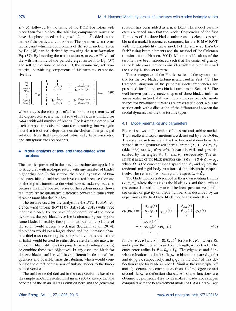
Table 1. Tuned parameters of simple model to fit the modal prop-erties of the DTU 10 MW RWT up to its 11th mode.
Parameter description Symbol Value
Blade length Lb 86.366 mFirst blade flap frequency ωf1 0.610 HzFirst blade edge frequency ωe 0.934 HzSecond blade flap frequency ωf2 1.738 HzHub radius Rh 2.8 mHub mass Mh 105 520 kgTower to rotor distance Ls 7.1 mGenerator inertia on low-speed shaft Ig 3 751 000 kg m2
Drivetrain stiffness Gs 0.668 GNm rad−1
Nacelle/effective tower mass M 446 040 kgNacelle tilt inertia Ix 4 106 000 kg m2
Nacelle roll inertia Iy 410 600 kg m2
Nacelle yaw inertia Iz 4 106 000 kg m2
Tower top side–side stiffness Kx 7.4 MN m−1
Tower top fore–aft stiffness Ky 7.4 MN m−1
Tower top tilt stiffness Gx 7.462 GNm rad−1
Tower top roll stiffness Gy 7.462 GNm rad−1
Tower top coupling stiffness gxy 0.2035 GNTower top yaw stiffness Gz 3.5 GNm rad−1
The ground-fixed substructure is modeled as a lumpedmass, and the inertia forces from the nacelle and effectivetower masses and the generator rotational inertia are derivedfrom the kinetic energy:
Tg =12M(ux + uy
)2+
12Ix θ
2x +
12Iy θ
2y +
12Izθ
2z +
12Igψ
2g , (44)
such that the first term of mg,0,ij in Eq. (A2) is replacedby ∂2 Tg/∂ui ∂uj . The potential energy for the linear elas-tic stiffnesses of the nacelle/tower motion, shaft torsion, andblade deflections is written as
V =12Kxu
2x +
12Kyu
2y +
12Gxθ
2x +
12Gyθ
2y +
12Gzθ
2z
− gxyθxuy + gxyθyux +12Gsψ
2s +
B∑k=1
Vbk , (45)
where Vbk is the potential energy of blade number k given as
Vbk =∑
β=[f1,e,f2]
12Mβω
2βq
2β,k +�
2∑
β=[f1,e,f2]
R∫0(∂2φx,β
∂z2
)2(∂2φy,β
∂z2
)2q2
β,k
R∫z
m(s)dsdz, (46)
where Mβ and ωβ are the modal mass and frequency of theorthogonal blade modes β = [f1, e, f2]. The last term is thepotential energy of the centrifugal forces proportional to thesquared rotor speed.
The damping matrices of Rayleigh’s dissipation functionin Eq. (10) for the blades Cb and the nacelle/tower motion
0 2 4 6 8 10 12 14 16 18 20 22 24
Number of harmonics [-]
10-15
10-10
10-5
100
105
2-no
rm o
f har
mon
ic c
ompo
nent
[s-1
]
Tw o-bladed rotorThree-bladed rotor
Figure 3. The 2-norms of the Fourier components of the systemmatrices for the two- and three-bladed simple models of the DTU10 MW RWT.
and shaft torsion Cg are set up using a spectral dampingmodel (Clough and Penzien, 1975). The first and second flap-wise blade modes are set to have logarithmic decrementsof 20 and 10 %, respectively, whereas all other modes aredamped 2–5 %. These choices of damping are simply crudeapproximations to the aeroelastic damping of the turbine inoperation (Bak et al., 2012), and they have no significant ef-fect on the results of Hill’s method. Damping is very impor-tant for solutions using Floquet theory where the system istime-integrated.
The linear equations of motion (Eq. 11) can be derivedfrom Eq. (7) and the integrals in Appendix A using the abovekinematic description of the blade motion, the kinetic energyof the nacelle/tower and generator inertia, the total potentialenergy, and the spectral damping matrices. For brevity, theblock matrices of Eq. (11) are not explicitly included. Allparameters (except for the blade properties in Fig. 2) of thetuned model are listed in Table 1.
4.2 Convergence of Fourier series for two-bladed rotor
Convergence of the Fourier series for the system ma-trix of two-bladed isotropic rotors is ensured if the con-stant part of the mass matrix for the ground-fixed DOFsis sufficiently larger then the second-order harmonic part.Using Eqs. (24) and (25), it can be computed that||Q−1
d QTs P0 Qs|| ≈ 0.22< 1 and ||Pk QT
s ||< 0.67 for k= 1,2, . . . , i.e., the inverse mass matrix and therefore the systemmatrix have finite Fourier series for the two-bladed rotor.
Figure 3 shows the 2-norms of the Fourier components ofthe system matrices for the models with the two- and three-bladed isotropic rotors. The convergence for the two-bladedrotor is observed and for the following analysis the numberof harmonics is chosen to be N = 7. The largest norm forthe 1/rev component is 46 480 s−1 and the largest norm of anomitted component (9/rev) is 0.03 s−1. For the three-bladedrotor all N = 3 harmonic components are used although thethird harmonic is effectively zero.
Wind Energ. Sci., 1, 271–296, 2016 www.wind-energ-sci.net/1/271/2016/

M. H. Hansen: Modal dynamics of structures with bladed isotropic rotors 281
0 2 4 6 8 10 12
Rotor speed [rpm]
0
0.2
0.4
0.6
0.8
1
1.2
1.4
1.6
1.8
2
Mod
al fr
eque
ncy
[Hz]
DT rotation
Tower fore-aftTower side-side
Sym flap 1
Anti flap 1
Anti edge 1
Anti flap 2
Sym edge 1Sym flap 2
0 2 4 6 8 10 12
Rotor speed [rpm]
0
0.2
0.4
0.6
0.8
1
1.2
1.4
1.6
1.8
2
Mod
al fr
eque
ncy
[Hz]
DT rotation
Tower fore-aftTower side-side
BW flap 1
Sym flap 1FW flap 1
BW edge 1
FW edge 1
BW flap 2
FW flap 2
Sym flap 2Sym edge 1
Figure 4. Campbell diagrams of the principal modal frequencies of the three-bladed (left plot) and two-bladed (right plot) version of theDTU 10 MW RWT computed with Hill’s method (circles) and with the software HAWCStab2 (crosses) for the three-bladed turbine.
4.3 Campbell diagrams of two- and three-bladedturbines
The number of harmonics in the periodic eigenvectors usedfor Hill’s truncated eigenvalue problem is set to M = 2N forboth rotors; thus, M = 14 and M = 6 for the two- and three-bladed rotor, respectively. The eigenvalue problem is solvedfor 33 equidistant rotor speeds ranging from 2 to 10 rpm(nominal speed of the DTU 10 MW RWT is 9.6 rpm). Theprincipal solutions at the lowest speed of 2 rpm are selectedamong the subsets of solutions as the one that has the largestmean component on the ground-fixed DOFs (see Sect. 3.2).For the remaining rotor speeds, the principal solutions are se-lected as the ones that have the largest modal assurance crite-rion relative to the principal solutions selected at the previousrotor speed.
Figure 4 shows the Campbell diagrams of principal modalfrequencies versus rotor speed for the three-bladed (left) andtwo-bladed (right) versions of the DTU 10 MW RWT. Themode names are deduced from the dominant components inthe periodic mode shapes (see Sects. 4.4 and 4.5). For thethree-bladed rotor, the principal modal frequencies computedwith Hill’s method (circles) are in close agreement with themodal frequencies computed with the high-fidelity softwareHAWCStab2 (crosses). This agreement shows that the sim-ple model combined with the automatic identification of theprincipal solutions is able to predict the same modal frequen-cies in the ground-fixed frame as computed using the Cole-man transformation method.
Comparison of the two Campbell diagrams shows that thetower modes of the two-bladed turbine have slightly higherfrequencies due to the lighter rotor. The ±1/rev frequencysplitting for the pairs of whirling rotor modes in the ground-fixed frame is clear for the three-bladed turbine (noting thatout-of-plane blade deflections are stiffened by the centrifu-gal forces). For the two-bladed turbine, there are no whirling
modes but the antisymmetric modes are still either increasing(first edge and flap) or decreasing (second flap) with 1/rev,because the principal solutions are selected as the solutionswith the largest mean components on ground-fixed DOFs.Campbell diagrams containing only the principal frequenciesare not very informative for two-bladed turbines. Instead, theperiodic mode shapes of the selected principal solutions arenow analyzed. Note that first mode of both turbines is thetrivial rigid-body rotation of the drivetrain, which is omittedfrom this analysis.
4.4 Periodic mode shapes of three-bladed turbines
Figures 5–15 show the dominant modal components of se-lected DOFs in the periodic mode shapes of the three-bladedturbine. The modal amplitudes are plotted as functions ofboth the rotor speed � and the frequency of the particu-lar component ω0+m�, where ω0 is the principal modalfrequency and m is the harmonic order of the component(see Eq. 34). Only amplitudes higher than 10 % of the over-all maximum amplitude across all rotor speeds are plotted.The generator rotation and shaft torsion angles are multipliedby 10 for better scaling of these small angles compared toblade deflections. Scaling of the tower translations are alsoapplied to show weak couplings for some modes. The plotlayout is the same in all figures: a three-dimensional plot inthe top and its projections onto the amplitude–rotor speed(left) and frequency–rotor speed (right) planes in the lowerplots. The principal frequencies ω0 are always denoted byblack filled circles in the frequency–rotor speed planes. Thecolor coding of the modal components is also the same inall figures: black markers denote amplitudes of ground-fixedDOFs. Red, green, and blue markers denote amplitudes ofthe rotor components of the first flapwise, first edgewise, andsecond flapwise deflection shapes, respectively, computedusing Eq. (39). Note that the frequency–rotor speed diagrams
www.wind-energ-sci.net/1/271/2016/ Wind Energ. Sci., 1, 271–296, 2016

282 M. H. Hansen: Modal dynamics of structures with bladed isotropic rotors
10
50
Modal frequencies [Hz]
2
0.5
0
Mod
al a
mpl
itude
s1.8 1.6 1.4 1.2 1 0.8 0.6 0.4 0.2 0
1
Rotor speed [rp
m]
FW flap 1 -1/revFore-aft +0/revSym flap 1 +0/revBW flap 1 +1/rev
0 2 4 6 8 10
Rotor speed [rpm]
0
0.5
1
1.5
2
Mod
al fr
eque
ncie
s [H
z]
0 2 4 6 8 10
Rotor speed [rpm]
0
0.2
0.4
0.6
0.8
1
Mod
al a
mpl
itude
s
Figure 5. Harmonic modal components for the three-bladed turbine mode dominated by tower fore–aft motion. Top panel: modal amplitudesplotted versus rotor speed and frequency of the particular harmonic component. Lower left panel: projection onto the plane of modal ampli-tudes and rotor speed. Lower right panel: projection onto the plane of component frequencies and rotor speed (periodic Campbell diagram).Filled black circles show the principal modal frequencies in the frequencies and rotor speed planes. Only modal components with amplitudeslarger than 10 % of the overall maximum amplitude are plotted.
10
50
Modal frequencies [Hz]
2
0.5
0
Mod
al a
mpl
itude
s
1.8 1.6 1.4 1.2 1 0.8 0.6 0.4 0.2 0
1
Rotor speed [rp
m]
FW edge 1 -1/revSide-side +0/rev10 x gen rot +0/revBW edge 1 +1/rev
0 2 4 6 8 10
Rotor speed [rpm]
0
0.5
1
1.5
2
Mod
al fr
eque
ncie
s [H
z]
0 2 4 6 8 10
Rotor speed [rpm]
0
0.2
0.4
0.6
0.8
1
Mod
al a
mpl
itude
s
Figure 6. Harmonic modal components for the three-bladed turbine mode dominated by tower side–side motion. Plot layout as in Fig. 5.
(lower right) are similar to the periodic Campbell diagramsin Bottasso and Cacciola (2015), except that each curve rep-resents the magnitude of the harmonic component for a par-ticular DOF and not the vector norm of all DOFs like theparticipation factors.
The naming of the modes shown in Fig. 4 is deduced fromthe harmonic components that dominate the periodic modeshapes observed in Figs. 5–15 across a large part of the rotor
speed range. Note that the first flapwise symmetric and for-ward whirling modes interchange their mode shapes at lowrotor speeds. The routine for sorting the modes based on amodal assurance criterion cannot always distinguish stronglycoupled modes from each other. This issue is dependent onthe resolution of the rotor speed range.
A general observation for the three-bladed turbine modesis that no harmonic component of the rotor response is
Wind Energ. Sci., 1, 271–296, 2016 www.wind-energ-sci.net/1/271/2016/

M. H. Hansen: Modal dynamics of structures with bladed isotropic rotors 283
10
50
Modal frequencies [Hz]
2
0.5
0
Mod
al a
mpl
itude
s1.8 1.6 1.4 1.2 1 0.8 0.6 0.4 0.2 0
1
Rotor speed [rp
m]
FW flap 1 -1/rev10 x fore-aft +0/revSym flap 1 +0/revBW flap 1 +1/rev
0 2 4 6 8 10
Rotor speed [rpm]
0
0.5
1
1.5
2
Mod
al fr
eque
ncie
s [H
z]
0 2 4 6 8 10
Rotor speed [rpm]
0
0.2
0.4
0.6
0.8
1
Mod
al a
mpl
itude
s
Figure 7. Harmonic modal components for the three-bladed turbine mode dominated by backward whirling (BW) of the rotor in the firstflapwise DOF. Plot layout as in Fig. 5.
10
50
Modal frequencies [Hz]
2
0.5
0
Mod
al a
mpl
itude
s
1.8 1.6 1.4 1.2 1 0.8 0.6 0.4 0.2 0
1
Rotor speed [rp
m]
FW flap 1 -1/rev10 x fore-aft +0/revSym flap 1 +0/revBW flap 1 +1/rev
0 2 4 6 8 10
Rotor speed [rpm]
0
0.5
1
1.5
2
Mod
al fr
eque
ncie
s [H
z]
0 2 4 6 8 10
Rotor speed [rpm]
0
0.2
0.4
0.6
0.8
1
Mod
al a
mpl
itude
s
Figure 8. Harmonic modal components for the three-bladed turbine mode dominated by symmetric deflection of the rotor in the first flapwiseDOF across the rotor speed range. Plot layout as in Fig. 5.
more than±1/rev from the principal frequency. Lowering thethreshold for the plotted amplitudes to 0.1 % of the overallmaximum amplitude did not change this observation. Thisagrees with Eq. (38) and previous studies of isotropic three-bladed turbines using the Coleman transformation method(Hansen, 2003, 2007): an inverse Coleman transformationfrom the ground-fixed frame with a single modal frequencyback to the rotating frame shows that symmetric componentswill have the same frequency as in the ground-fixed frame,but BW and FW components will have frequencies that are
+1/rev and −1/rev, respectively, from a principal frequencydefined in the ground-fixed frame. If the three-bladed rotorwas anisotropic, then secondary harmonics will arise whosemagnitudes will depend on the magnitude of the anisotropy(Skjoldan and Hansen, 2009).
Looking at the individual mode shapes, there are couplingsof the different DOFs in each mode of three-bladed turbines.The tower fore–aft mode (Fig. 5) contains symmetric, BW,and FW components in the first flapwise blade mode. Sim-ilarly, the tower side–side mode (Fig. 6) contains BW and
www.wind-energ-sci.net/1/271/2016/ Wind Energ. Sci., 1, 271–296, 2016

284 M. H. Hansen: Modal dynamics of structures with bladed isotropic rotors
10
50
Modal frequencies [Hz]
2
0.5
0
Mod
al a
mpl
itude
s1.8 1.6 1.4 1.2 1 0.8 0.6 0.4 0.2 0
1
Rotor speed [rp
m]
FW flap 1 -1/rev10 x fore-aft +0/revSym flap 1 +0/revBW flap 1 +1/revBW edge 1 +1/rev
0 2 4 6 8 10
Rotor speed [rpm]
0
0.5
1
1.5
2
Mod
al fr
eque
ncie
s [H
z]
0 2 4 6 8 10
Rotor speed [rpm]
0
0.2
0.4
0.6
0.8
1
Mod
al a
mpl
itude
s
Figure 9. Harmonic modal components for the three-bladed turbine mode dominated by forward whirling (FW) of the rotor in the firstflapwise DOF across the rotor speed range. Plot layout as in Fig. 5.
10
50
Modal frequencies [Hz]
2
0.5
0
Mod
al a
mpl
itude
s
1.8 1.6 1.4 1.2 1 0.8 0.6 0.4 0.2 0
1
Rotor speed [rp
m]
FW flap 1 -1/revFW edge 1 -1/rev10 x fore-aft +0/rev10 x side-side +0/revSym flap 1 +0/revBW flap 1 +1/revBW edge 1 +1/rev
0 2 4 6 8 10
Rotor speed [rpm]
0
0.5
1
1.5
2
Mod
al fr
eque
ncie
s [H
z]
0 2 4 6 8 10
Rotor speed [rpm]
0
0.2
0.4
0.6
0.8
1
Mod
al a
mpl
itude
s
Figure 10. Harmonic modal components for the three-bladed turbine mode dominated by backward whirling (BW) of the rotor in theedgewise DOF. Plot layout as in Fig. 5.
FW components in the first edgewise blade mode and gen-erator rotation due to the nacelle roll. The first BW flap-wise mode (Fig. 7) is not pure and also contains symmetricand FW components. The strongly coupled first symmetric(Fig. 8) and FW (Fig. 9) flapwise modes are also not pureand contain other components as well. Note that a BW edge-wise component (in green) appears in the first FW flapwisemode at the highest rotor speeds where its BW flapwise com-ponent approaches the edgewise blade frequency of about0.93 Hz. Similarly, the FW flapwise components appear in
the first BW edgewise mode (Fig. 10) at higher rotor speeds.The first FW edgewise mode (Fig. 11) contains a small BWedgewise component and a larger FW flapwise component.Similar couplings can be seen for the remaining modes. Thesecond flapwise whirling modes (Figs. 12 and 13) have thelargest blade response at a frequency of about 1.5 Hz (the+1/rev for BW and −1/rev for the FW components). Theamplitude ratio of these flapwise DOFs are almost constant,indicating that the rotor modes are constructed as a combina-tion of the two blade modes with the isolated modal frequen-
Wind Energ. Sci., 1, 271–296, 2016 www.wind-energ-sci.net/1/271/2016/

M. H. Hansen: Modal dynamics of structures with bladed isotropic rotors 285
10
50
Modal frequencies [Hz]
2
0.5
0
Mod
al a
mpl
itude
s1.8 1.6 1.4 1.2 1 0.8 0.6 0.4 0.2 0
1
Rotor speed [rp
m]
FW flap 1 -1/revFW edge 1 -1/rev10 x side-side +0/revBW edge 1 +1/rev
0 2 4 6 8 10
Rotor speed [rpm]
0
0.5
1
1.5
2
Mod
al fr
eque
ncie
s [H
z]
0 2 4 6 8 10
Rotor speed [rpm]
0
0.2
0.4
0.6
0.8
1
Mod
al a
mpl
itude
s
Figure 11. Harmonic modal components for the three-bladed turbine mode dominated by forward whirling (FW) of the rotor in the edgewiseDOF. Plot layout as in Fig. 5.
10
50
Modal frequencies [Hz]
2
0.5
0
Mod
al a
mpl
itude
s
1.8 1.6 1.4 1.2 1 0.8 0.6 0.4 0.2 0
1
Rotor speed [rp
m]
FW flap 1 -1/revFW edge 1 -1/revFW flap 2 -1/rev10 x side-side +0/revBW flap 1 +1/revBW edge 1 +1/revBW flap 2 +1/rev
0 2 4 6 8 10
Rotor speed [rpm]
0
0.5
1
1.5
2
Mod
al fr
eque
ncie
s [H
z]
0 2 4 6 8 10
Rotor speed [rpm]
0
0.2
0.4
0.6
0.8
1
Mod
al a
mpl
itude
s
Figure 12. Harmonic modal components for the three-bladed turbine mode dominated by backward whirling (BW) of the rotor in the secondflapwise DOF. Plot layout as in Fig. 5.
cies 0.61 and 1.74 Hz. The first symmetric edgewise mode(Fig. 15) couples with both the generator rotation and theshaft torsion, but not with any whirling components. Thesecond symmetric flapwise mode (Fig. 14) contains whirlingcomponents that are just below the selected threshold for theplotted amplitudes and therefore not shown.
4.5 Periodic mode shapes of two-bladed turbines
Figures 16–23 show the dominant modal components of se-lected DOFs in the periodic mode shapes of the two-bladedturbine. The scaling of DOF amplitudes, plot layout, andcolor coding are the same as for the three-bladed turbine. Theamplitudes of rotor motion are again computed from the pe-riodic eigenvector using Eq. (39).
A general observation for the two-bladed turbine modes isthe larger amplitudes and the higher order of the harmoniccomponents compared to the three-bladed turbine. Another
www.wind-energ-sci.net/1/271/2016/ Wind Energ. Sci., 1, 271–296, 2016
286 M. H. Hansen: Modal dynamics of structures with bladed isotropic rotors
10
50
Modal frequencies [Hz]
2
0.5
0
Mod
al a
mpl
itude
s1.8 1.6 1.4 1.2 1 0.8 0.6 0.4 0.2 0
1
Rotor speed [rp
m]
FW flap 1 -1/revFW edge 1 -1/revFW flap 2 -1/rev10 x fore-aft +0/revSym flap 2 +0/revBW flap 1 +1/revBW flap 2 +1/rev
0 2 4 6 8 10
Rotor speed [rpm]
0
0.5
1
1.5
2
Mod
al fr
eque
ncie
s [H
z]
0 2 4 6 8 10
Rotor speed [rpm]
0
0.2
0.4
0.6
0.8
1
Mod
al a
mpl
itude
s
Figure 13. Harmonic modal components for the mode dominated by forward whirling (FW) of the rotor in the second flapwise DOF. Plotlayout as in Fig. 5.
observation is that symmetric rotor components always havefrequencies that are an even number of 1/rev away from theprincipal frequency, whereas frequencies for antisymmetriccomponents are shifted an odd number.
Looking at the individual mode shapes, the increased num-ber of harmonics also increases the number of couplings be-tween the different DOFs in each mode. The tower fore–aftmode in Fig. 16 couples again with ±1/rev asymmetric rotormotion as for the three-bladed turbine. However, couplingsto higher harmonic components of the blade DOFs are muchmore dominant at rotor speeds where their frequency crossesthe corresponding blade frequency. Such resonant couplingsoccur for the symmetric +4/rev and +6/rev components andantisymmetric +3/rev and +5/rev components of the firstflapwise DOF when their frequencies are close to the firstflapwise blade frequency, 0.61 Hz, as well as for the antisym-metric+5/rev component of the first edgewise DOF when itsfrequency crosses 0.93 Hz.
The tower side–side mode in Fig. 17 is similar to the samemode of the three-bladed turbine with the coupling to thegenerator rotation and the ±1/rev harmonics of asymmetricrotor responses.
The symmetric and antisymmetric flapwise modes inFigs. 18 and 19 interchange mode shapes at low rotor speeds;however, they are here named after their dominant compo-nents at the higher rotor speeds. The antisymmetric flapwisemode couples with tower fore–aft motion around 6.5 rpm,where the frequency of the −4/rev component of this DOFis crossing the tower fore–aft frequency of about 0.28 Hz.A similar coupling is seen for the −6/rev component of thetower fore–aft DOF in the antisymmetric edgewise modein Fig. 20 at 8.2 rpm. This mode also contains 0/rev and
−2/rev components of the tower side–side DOF such thatthe ±1/rev splitting known from three-bladed rotors appearsin the ground-fixed frame.
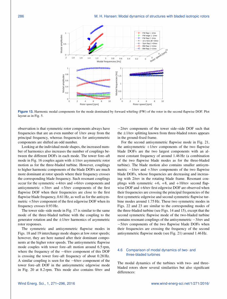
For the second antisymmetric flapwise mode in Fig. 21,the antisymmetric +1/rev components of the two flapwiseblade DOFs are the two largest components with an al-most constant frequency of around 1.46 Hz (a combinationof the two flapwise blade modes as for the three-bladedturbine). The blade motion also contains smaller antisym-metric −1/rev and +3/rev components of the two flapwiseblade DOFs, whose frequencies are decreasing and increas-ing with 2/rev in the rotating blade frame. Resonant cou-plings with symmetric +6, +8, and +10/rev second flap-wise DOF and+6/rev first edgewise DOF are observed whentheir frequencies are crossing the principal frequencies of thefirst symmetric edgewise and second symmetric flapwise tur-bine modes around 1.75 Hz. These two symmetric modes inFigs. 22 and 23 are similar to the corresponding modes ofthe three-bladed turbine (see Figs. 14 and 15), except that thesecond symmetric flapwise mode of the two-bladed turbinecontains resonant couplings of the antisymmetric−3/rev and−5/rev components of the two flapwise blade DOFs whentheir frequencies are crossing the frequency of the secondantisymmetric flapwise mode (see Fig. 21) around 1.46 Hz.
4.6 Comparison of modal dynamics of two- andthree-bladed turbines
The modal dynamics of the turbines with two- and three-bladed rotors show several similarities but also significantdifferences:
Wind Energ. Sci., 1, 271–296, 2016 www.wind-energ-sci.net/1/271/2016/

M. H. Hansen: Modal dynamics of structures with bladed isotropic rotors 287
10
50
Modal frequencies [Hz]
2
0.5
0
Mod
al a
mpl
itude
s1.8 1.6 1.4 1.2 1 0.8 0.6 0.4 0.2 0
1
Rotor speed [rp
m]
Sym edge 1 +0/revSym flap 2 +0/rev
0 2 4 6 8 10
Rotor speed [rpm]
0
0.5
1
1.5
2
Mod
al fr
eque
ncie
s [H
z]
0 2 4 6 8 10
Rotor speed [rpm]
0
0.2
0.4
0.6
0.8
1
Mod
al a
mpl
itude
s
Figure 14. Harmonic modal components for the mode dominated by symmetric deflection of the rotor in the second flapwise mode. Plotlayout as in Fig. 5.
10
50
Modal frequencies [Hz]
2
0.5
0
Mod
al a
mpl
itude
s
1.8 1.6 1.4 1.2 1 0.8 0.6 0.4 0.2 0
1
Rotor speed [rp
m]
10 x gen rot +0/rev10 x shaft tors +0/revSym flap 1 +0/revSym edge 1 +0/revSym flap 2 +0/rev
0 2 4 6 8 10
Rotor speed [rpm]
0
0.5
1
1.5
2
Mod
al fr
eque
ncie
s [H
z]
0 2 4 6 8 10
Rotor speed [rpm]
0
0.2
0.4
0.6
0.8
1
Mod
al a
mpl
itude
s
Figure 15. Harmonic modal components for the mode dominated by symmetric deflection of the rotor in the edgewise mode. Plot layout asin Fig. 5.
– The rigid-body drivetrain rotation mode (trivial andtherefore not shown) is identical for the two turbines.
– Tower bending modes are similar in frequencies andshapes, except that the fore–aft mode for the two-bladedturbine may contain large components of the first flap-wise blade mode when the rotor speed is such thatthese frequencies of the higher harmonic componentsare crossing the modal frequency of this blade mode.
– The first symmetric edgewise rotor mode is very similarin frequency and shape because its reaction forces donot couple to other DOFs through large periodic termsin the system matrix.
– The symmetric flapwise rotor modes are similar in fre-quency and shape, except that the first symmetric flap-wise mode of the two-bladed turbine in Fig. 18 has asmall -2/rev component of the tower fore–aft DOF, andthe second symmetric flapwise mode in Fig. 23 has res-onant couplings to antisymmetric flapwise mode.
www.wind-energ-sci.net/1/271/2016/ Wind Energ. Sci., 1, 271–296, 2016

288 M. H. Hansen: Modal dynamics of structures with bladed isotropic rotors
10
50
Modal frequencies [Hz]
2
0.5
0
Mod
al a
mpl
itude
s1.8 1.6 1.4 1.2 1 0.8 0.6 0.4 0.2 0
1
Rotor speed [rp
m]
Anti flap 1 -1/revFore-aft +0/revSym flap 1 +0/revAnti flap 1 +1/revSym flap 1 +2/revAnti flap 1 +3/revSym flap 1 +4/revAnti flap 1 +5/revAnti edge 1 +5/revSym flap 1 +6/rev
0 2 4 6 8 10
Rotor speed [rpm]
0
0.5
1
1.5
2
Mod
al fr
eque
ncie
s [H
z]
0 2 4 6 8 10
Rotor speed [rpm]
0
0.2
0.4
0.6
0.8
1
Mod
al a
mpl
itude
s
Figure 16. Harmonic modal components for the two-bladed turbine mode dominated by tower fore–aft motion. Plot layout as in Fig. 5.
10
50
Modal frequencies [Hz]
2
0.5
0
Mod
al a
mpl
itude
s
1.8 1.6 1.4 1.2 1 0.8 0.6 0.4 0.2 0
1
Rotor speed [rp
m]
Anti edge 1 -1/revSide-side +0/rev10 x gen rot +0/revAnti edge 1 +1/rev
0 2 4 6 8 10
Rotor speed [rpm]
0
0.5
1
1.5
2
Mod
al fr
eque
ncie
s [H
z]
0 2 4 6 8 10
Rotor speed [rpm]
0
0.2
0.4
0.6
0.8
1
Mod
al a
mpl
itude
s
Figure 17. Harmonic modal components for the two-bladed turbine mode dominated by tower side–side motion. Plot layout as in Fig. 5.
– Asymmetric rotor modes: the antisymmetric modes forthe two-bladed turbine and the whirling mode pairs ofthe three-bladed turbine may seem similar when ob-served from the ground-fixed frame such as a top toweracceleration signal, where the well-known ±1/rev split-ting of the frequency peaks is seen. For example, thetower side–side responses at ±1/rev around the bladeedgewise frequency is observed for both the antisym-metric edgewise mode in Fig. 20 and for the edgewisewhirling mode pair in Figs. 10 and 11. This similarityhas probably caused the misinterpretation of the sim-ulated and measured two-bladed responses in Kim et
al. (2015) and Larsen and Kim (2015), but rotor modesof a two-bladed turbine will often have more frequencypeaks in both the ground-fixed frame and the rotatingblade frame.
The additional modal couplings that exist for two-bladed tur-bines have the effect that there are additional ways that themodes can be excited by either resonances or interactionswith external forces, and that it becomes difficult to interpretfrequency spectra from simulations and measurements. To il-lustrate these effects, the harmonic components of the towerside–side DOF in all modes are plotted in three-dimensionalperiodic Campbell diagrams for both turbines in Fig. 24.
Wind Energ. Sci., 1, 271–296, 2016 www.wind-energ-sci.net/1/271/2016/

M. H. Hansen: Modal dynamics of structures with bladed isotropic rotors 289
10
50
Modal frequencies [Hz]
2
0.5
0
Mod
al a
mpl
itude
s1.8 1.6 1.4 1.2 1 0.8 0.6 0.4 0.2 0
1
Rotor speed [rp
m]
Anti flap 1 -3/rev10 x fore-aft -2/revAnti flap 1 -1/rev10 x fore-aft +0/revSym flap 1 +0/revAnti flap 1 +1/rev
0 2 4 6 8 10
Rotor speed [rpm]
0
0.5
1
1.5
2
Mod
al fr
eque
ncie
s [H
z]
0 2 4 6 8 10
Rotor speed [rpm]
0
0.2
0.4
0.6
0.8
1
Mod
al a
mpl
itude
s
Figure 18. Harmonic modal components for the two-bladed turbine mode dominated by symmetric deflection of the rotor in the first flapwiseDOF across the rotor speed range. Plot layout as in Fig. 5.
10
50
Modal frequencies [Hz]
2
0.5
0
Mod
al a
mpl
itude
s
1.8 1.6 1.4 1.2 1 0.8 0.6 0.4 0.2 0
1
Rotor speed [rp
m]
10 x fore-aft -4/revAnti flap 1 -3/rev10 x fore-aft -2/revAnti flap 1 -1/rev10 x fore-aft +0/revSym flap 1 +0/revAnti flap 1 +1/revAnti edge 1 +1/rev
0 2 4 6 8 10
Rotor speed [rpm]
0
0.5
1
1.5
2
Mod
al fr
eque
ncie
s [H
z]
0 2 4 6 8 10
Rotor speed [rpm]
0
0.2
0.4
0.6
0.8
1
Mod
al a
mpl
itude
s
Figure 19. Harmonic modal components for the two-bladed turbine mode dominated by antisymmetric deflection of the rotor in the firstflapwise DOF across the rotor speed range. Plot layout as in Fig. 5.
These plots show qualitatively the response in a tower side–side signal when all modes are excited equally. There areclear similarities between the dominant side–side responsesfor the two turbines. However, where these responses in theground-fixed frame for the three-bladed turbine only occuron the principal modal frequencies plotted in its conventionalCampbell diagram (see Fig. 4), the modes of two-bladed tur-bine lead to responses in the ground-fixed frame at manyother frequencies. The conventional Campbell diagram con-taining only the principal modal frequencies of a two-bladed
turbine therefore has little value, and one should be carefulwhen interpreting frequency response plots for two-bladedturbines.
5 Conclusions
The modal dynamics of structures with bladed isotropic ro-tors (identical and equidistantly spaced blades) have been an-alyzed using the periodic mode shapes obtained using Hill’smethod on the linear periodic first-order system equation.
www.wind-energ-sci.net/1/271/2016/ Wind Energ. Sci., 1, 271–296, 2016
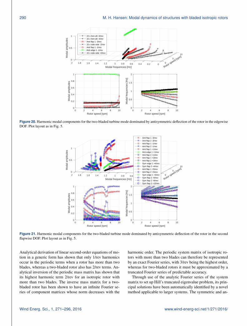
290 M. H. Hansen: Modal dynamics of structures with bladed isotropic rotors
10
50
Modal frequencies [Hz]
2
0.5
0
Mod
al a
mpl
itude
s1.8 1.6 1.4 1.2 1 0.8 0.6 0.4 0.2 0
1
Rotor speed [rp
m]
15 x fore-aft -6/rev15 x fore-aft -4/revAnti flap 1 -3/rev15 x side-side -2/revAnti flap 1 -1/revAnti edge 1 -1/rev15 x side-side +0/rev
0 2 4 6 8 10
Rotor speed [rpm]
0
0.5
1
1.5
2
Mod
al fr
eque
ncie
s [H
z]
0 2 4 6 8 10
Rotor speed [rpm]
0
0.2
0.4
0.6
0.8
1
Mod
al a
mpl
itude
s
Figure 20. Harmonic modal components for the two-bladed turbine mode dominated by antisymmetric deflection of the rotor in the edgewiseDOF. Plot layout as in Fig. 5.
10
50
Modal frequencies [Hz]
2
0.5
0
Mod
al a
mpl
itude
s
1.8 1.6 1.4 1.2 1 0.8 0.6 0.4 0.2 0
1
Rotor speed [rp
m]
Anti flap 1 -3/revAnti flap 2 -3/revAnti flap 1 -1/revAnti flap 2 -1/revAnti flap 1 +1/revAnti edge 1 +1/revAnti flap 2 +1/revAnti flap 1 +3/revAnti flap 2 +3/revSym edge 1 +4/revSym flap 2 +4/revAnti flap 1 +5/revAnti flap 2 +5/revSym edge 1 +6/revSym flap 2 +6/revSym flap 2 +8/revSym flap 2 +10/rev
0 2 4 6 8 10
Rotor speed [rpm]
0
0.5
1
1.5
2
Mod
al fr
eque
ncie
s [H
z]
0 2 4 6 8 10
Rotor speed [rpm]
0
0.2
0.4
0.6
0.8
1
Mod
al a
mpl
itude
s
Figure 21. Harmonic modal components for the two-bladed turbine mode dominated by antisymmetric deflection of the rotor in the secondflapwise DOF. Plot layout as in Fig. 5.
Analytical derivation of linear second-order equations of mo-tion in a generic form has shown that only 1/rev harmonicsoccur in the periodic terms when a rotor has more than twoblades, whereas a two-bladed rotor also has 2/rev terms. An-alytical inversion of the periodic mass matrix has shown thatits highest harmonic term 2/rev for an isotropic rotor withmore than two blades. The inverse mass matrix for a two-bladed rotor has been shown to have an infinite Fourier se-ries of component matrices whose norm decreases with the
harmonic order. The periodic system matrix of isotropic ro-tors with more than two blades can therefore be representedby an exact Fourier series, with 3/rev being the highest order,whereas for two-bladed rotors it must be approximated by atruncated Fourier series of predictable accuracy.
Through use of the analytic Fourier series of the systemmatrix to set up Hill’s truncated eigenvalue problem, its prin-cipal solutions have been automatically identified by a novelmethod applicable to larger systems. The symmetric and an-
Wind Energ. Sci., 1, 271–296, 2016 www.wind-energ-sci.net/1/271/2016/

M. H. Hansen: Modal dynamics of structures with bladed isotropic rotors 291
10
50
Modal frequencies [Hz]
2
0.5
0
Mod
al a
mpl
itude
s1.8 1.6 1.4 1.2 1 0.8 0.6 0.4 0.2 0
1
Rotor speed [rp
m]
10 x gen rot +0/rev10 x shaft tors +0/revSym flap 1 +0/revSym edge 1 +0/revSym flap 2 +0/rev
0 2 4 6 8 10
Rotor speed [rpm]
0
0.5
1
1.5
2
Mod
al fr
eque
ncie
s [H
z]
0 2 4 6 8 10
Rotor speed [rpm]
0
0.2
0.4
0.6
0.8
1
Mod
al a
mpl
itude
s
Figure 22. Harmonic modal components for the two-bladed turbine mode dominated by symmetric deflection of the rotor in the edgewiseDOF for the higher rotor speeds. Plot layout as in Fig. 5.
10
50
Modal frequencies [Hz]
2
0.5
0
Mod
al a
mpl
itude
s
1.8 1.6 1.4 1.2 1 0.8 0.6 0.4 0.2 0
1
Rotor speed [rp
m]
Anti flap 1 -5/revAnti flap 2 -5/revAnti flap 1 -3/revAnti flap 2 -3/rev10 x gen rot +0/rev10 x shaft tors +0/revSym edge 1 +0/revSym flap 2 +0/rev
0 2 4 6 8 10
Rotor speed [rpm]
0
0.5
1
1.5
2
Mod
al fr
eque
ncie
s [H
z]
0 2 4 6 8 10
Rotor speed [rpm]
0
0.2
0.4
0.6
0.8
1
Mod
al a
mpl
itude
s
Figure 23. Harmonic modal components for the two-bladed turbine mode dominated by symmetric deflection of the rotor in the secondflapwise DOF. Plot layout as in Fig. 5.
tisymmetric modal components of rotors with two bladesand the additional whirling components of rotors with moreblades have been extracted directly from the periodic eigen-vector corresponding to each principal eigen-solution.
As relevant examples, the generic methods have been usedto model and analyze the modal dynamics of both two- andthree-bladed versions of a 10 MW turbine. The motion ofeach blade has been described by its three first mode shapes,and the nacelle motion and drivetrain rotations have been de-scribed by seven DOFs. Similarities and significant differ-
ences between the modal dynamics of the turbines with two-and three-bladed rotors have been found and summarized inSect. 4.6. A difference is that the larger number and magni-tudes of the harmonic components in the system matrix oftwo-bladed turbines leads to resonant couplings in the modeshapes that have not been observed for the three-bladed tur-bine. These couplings between DOFs arise when the rotorspeed is such that the frequency of a higher harmonic com-ponent of one turbine mode is in the vicinity of the frequencyof another blade or turbine mode. Another difference is that
www.wind-energ-sci.net/1/271/2016/ Wind Energ. Sci., 1, 271–296, 2016
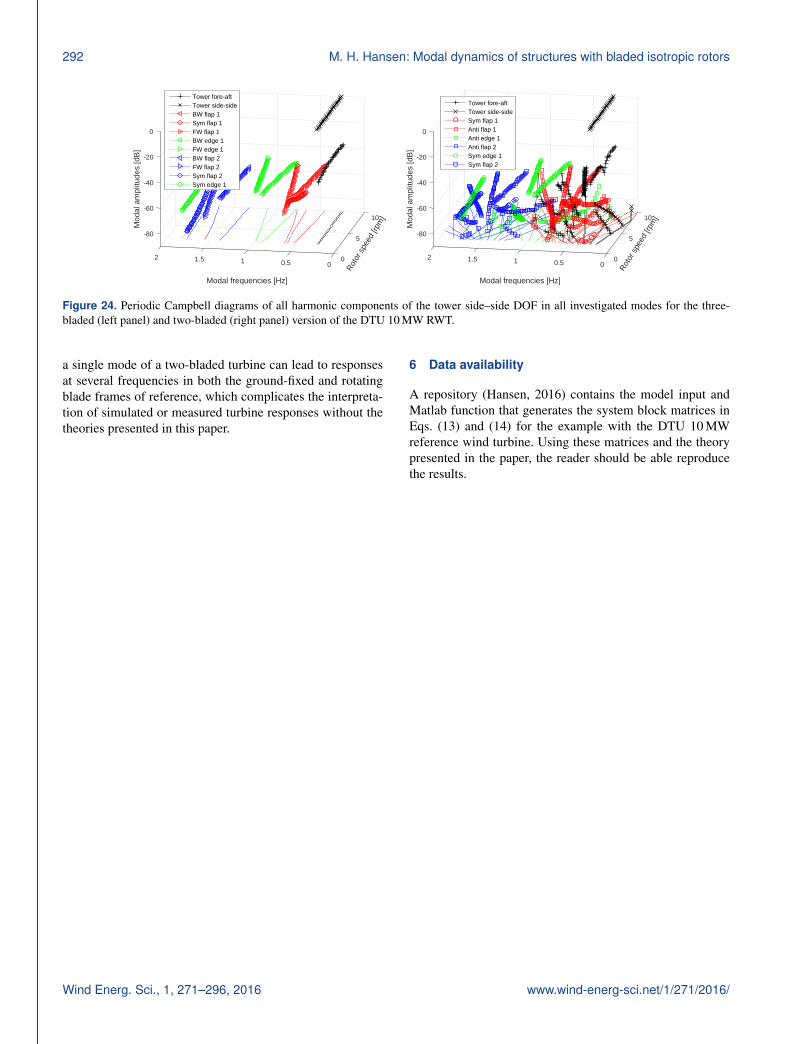
292 M. H. Hansen: Modal dynamics of structures with bladed isotropic rotors
10
5-80
Modal frequencies [Hz]
-60
2 1.5 0
Mod
al a
mpl
itude
s [d
B]
-40
1 0.5
-20
0
0
Rot
or s
peed
[rpm
]
Tower fore-aftTower side-sideSym flap 1Anti flap 1Anti edge 1Anti flap 2Sym edge 1Sym flap 2
10
5-80
Modal frequencies [Hz]
-60
2 1.5 0
Mod
al a
mpl
itude
s [d
B]
-40
1 0.5
-20
0
0
Rot
or s
peed
[rpm
]
Tower fore-aftTower side-sideBW flap 1Sym flap 1FW flap 1BW edge 1FW edge 1BW flap 2FW flap 2Sym flap 2Sym edge 1
Figure 24. Periodic Campbell diagrams of all harmonic components of the tower side–side DOF in all investigated modes for the three-bladed (left panel) and two-bladed (right panel) version of the DTU 10 MW RWT.
a single mode of a two-bladed turbine can lead to responsesat several frequencies in both the ground-fixed and rotatingblade frames of reference, which complicates the interpreta-tion of simulated or measured turbine responses without thetheories presented in this paper.
6 Data availability
A repository (Hansen, 2016) contains the model input andMatlab function that generates the system block matrices inEqs. (13) and (14) for the example with the DTU 10 MWreference wind turbine. Using these matrices and the theorypresented in the paper, the reader should be able reproducethe results.
Wind Energ. Sci., 1, 271–296, 2016 www.wind-energ-sci.net/1/271/2016/
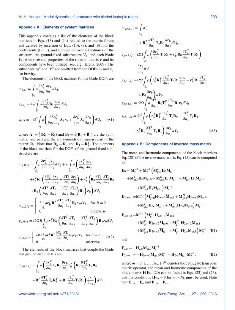
M. H. Hansen: Modal dynamics of structures with bladed isotropic rotors 293
Appendix A: Elements of system matrices
This appendix contains a list of the elements of the blockmatrices in Eqs. (13) and (14) related to the inertia forcesand derived by insertion of Eqs. (10), (8), and (9) into thecoefficients (Eq. 7), and summation over all volumes of thestructure, the ground-fixed substructure Vg , and each bladeVb, where several properties of the rotation matrix r and itscomponents have been utilized (see, e.g., Krenk, 2009). Thesubscripts “g” and “b” are omitted from the DOFs ui and ujfor brevity.
The elements of the block matrices for the blade DOFs are
mb,ij =
∫Vb
ρ∂rTb∂ui
∂rb
∂ujdVb
gb,ij = 4�∫Vb
ρ∂rTb∂ui
B1∂rb
∂ujdVb
sb,ij =−�2∫Vb
ρ
(∂2rTb∂ui∂uj
A1rb+∂rTb∂ui
A1∂rb
∂uj
)dVb, (A1)
where A1=12 (R1−R1) and B1=
12 (R1+R1) are the sym-
metric real part and the antisymmetric imaginary part of thematrix R1. Note that RT0 =R0 and R1=RT1 . The elementsof the block matrices for the DOFs of the ground-fixed sub-structure are
mg,0,ij =
∫Vg
ρ∂rTg
∂ui
∂rg
∂ujdVg+B
∫Vb
ρ
(∂rTc∂ui
∂rc
∂uj
+rTb R0
(∂TTc∂ui
∂rc
∂uj+∂TTc∂uj
∂rc
∂ui
)+ rTb
(R0∂TTc∂ui
∂Tc
∂ujR0
+R1
(∂TTc∂ui
∂Tc
∂uj+∂TTc∂uj
∂Tc
∂ui
)R1
)rb
)dVb
mg,2,ij =
2∫Vb
ρrTb RT1∂TTc∂ui
∂Tc
∂ujR1rbdVb for B = 2
0 otherwise
gg,0,ij = ι2�B∫Vb
ρrTb R1
(∂TTc∂ui
∂Tc
∂uj−∂TTc∂uj
∂Tc
∂ui
)R1rbdVb
gg,2,ij =
ι4�∫Vb
ρrTb RT1∂TTc∂ui
∂Tc
∂ujR1rbdVb for B = 2
0 otherwise. (A2)
The elements of the block matrices that couple the bladeand ground-fixed DOFs are
mgb,0,ij =
∫Vb
ρ
(∂rTc∂ui
TcR0∂rb
∂ujrTb
(R0∂TTc∂ui
TcR0
+RT1∂TTc∂ui
TcRT1 +R1∂TTc∂ui
TcR1
)∂rb
∂uj
)dVb
mgb,1,ij =
∫Vb
ρ (
. . .+RT1∂TTc∂ui
TcR0∂rb
∂ujdVb,
ggb,1,ij =ι2�∫Vb
ρ
(∂rTc∂ui
TcR1+ rTb R0∂TTc∂ui
TcR1
)∂rb
∂ujdVb
gbg,0,ij =ι2�∫Vb
ρ
(rTb RT1
∂TTc∂uj
TcR1∂rb
∂ui− rTb R1
∂TTc∂uj
TcR1∂rb
∂ui
)dVb
gbg,1,ij = ι2�∫Vb
ρ∂rTb∂ui
R0TTc∂Tc
∂ujR1rbdVb
sgb,1,ij =�2∫Vb
ρ
(rTb RT1
∂TTc∂ui
TcR0−∂rTc∂ui
TcR1
−rTb R0∂TTc∂ui
TcR1
)∂rb
∂ujdVb. (A3)
Appendix B: Components of inverted mass matrix
The mean and harmonic components of the block matricesEq. (28) of the inverse mass matrix Eq. (15) can be computedas
E0 =M−1r +M−1
r
(MH
gr,1H2Mgr,1
+MTgr,0H0Mgr,0+MH
gr,1H0Mgr,1+MTgr,1H0Mgr,1
+MTgr,1H2Mgr,1
)M−1
r
E2m+1 =M−1r
(MT
gr,0H2m+2Mgr,1+MHgr,1H2m+2Mgr,0
+MTgr,0H2mMgr,1+MT
gr,1H2mMgr,0
)M−1
r
E2m+2 =M−1r
(MH
gr,1H2m+4Mgr,1
+MTgr,0H2m+2Mgr,0+MH
gr,1H2m+2Mgr,1
+MTgr,1H2m+2Mgr,1+MT
gr,1H2mMgr,1
)M−1
r (B1)
and
F2m =−H2mMgr,0M−1r
F2m+1 =−H2m+2Mgr,1M−1r −H2mMgr,1M−1
r , (B2)
wherem= 0, 1, . . . ,Nh, (·)H denotes the conjugate transposematrix operator, the mean and harmonic components of theblock matrix H Eq. (20) can be found in Eqs. (22) and (23),and the conditions H2m= 0 for m>Nh must be used. Notethat E−n=En and F−n=Fn.
www.wind-energ-sci.net/1/271/2016/ Wind Energ. Sci., 1, 271–296, 2016

294 M. H. Hansen: Modal dynamics of structures with bladed isotropic rotors
Appendix C: Components of system matrix
The components of the system matrix Eq. (29) can be writtenas
An =
[0 A12
A21,11,n A21,12,nA21,21,n A21,22,n
A22,11,n A22,12,nA22,21,n A22,22,n
], (C1)
where A12= I for n= 0 and A12= 0 for n> 0, and the blockmatrices can be computed as
A21,11,n =−En (Kr+Sr)−FTn−1Sgr,1−FTn+1Sgr,1
A21,21,n =−Fn (Kr+Sr)−HTn−1Sgr,1−HT
n+1Sgr,1
A21,12,n =−FTnKg
A21,22,n =−HnKg
A22,11,n =−EnCr−FTnGgr,0−FTn−1Ggr,1−FTn+1Ggr,1
A22,21,n =−FnCr−HnGgr,0−Hn−1Ggr,1−Hn+1Ggr,1
A22,12,n =−FTn(Gg,0+Cg
)−En−1Grg,1−En+1Grg,1
−FTn−2Gg,2−FTn+2Gg,2
A22,22,n =−Hn
(Gg,0+Cg
)−Fn−1Grg,1−Fn+1Grg,1
−Hn−2Gg,2−Hn+2Gg,2 (C2)
for n= 0, 1, . . . , 2Nh+ 3 using the following properties ofthe matrices En, Fn, and Hn:
E−n = En, E−n = En, H−n =Hn, andEn+2 = Fn+1 =Hn = 0 for n > 2Nh.
Note that Nh= 0 for isotropic rotors with more than twoblades, whereas Nh is selected for two-bladed rotors basedon the required accuracy of the system matrix.
Wind Energ. Sci., 1, 271–296, 2016 www.wind-energ-sci.net/1/271/2016/
M. H. Hansen: Modal dynamics of structures with bladed isotropic rotors 295
Acknowledgements. The support by the Danish Energy Agencythrough the EUDP-2011 II project “Demonstration of PartialPitch 2-Bladed Wind Turbine Performance” is gratefully acknowl-edged. The author would also like to thank Anders M. Hansen,Ilmar F. Santos, Torben J. Larsen, Riccardo Riva, and projectpartners at Envision Energy for valuable discussions.
Edited by: A. KoliosReviewed by: V. A. Riziotis and D. Ossmann
References
Allemang, R. J.: The Modal Assurance Criterion – Twenty years ofuse and abuse, Sound Vibrat., 37, 14–21, 2003.
Bak, C., Bitsche, R., Yde, A., Kim, T., Hansen, M. H., Zahle, F.,Gaunaa, M., Blasques, J. P. A. A., Døssing, M., Wedel Heinen,J. J., and Behrens, T.: Light Rotor: The 10-MW reference windturbine, European Wind Energy Association Conference and Ex-hibition, 16–19 April 2012, Copenhagen, Denmark, 2012.
Bergami, L. and, Hansen, M. H.: High-fidelity linear time-invariantmodel of a smart rotor with adaptive trailing edge flaps, WindEnergy., doi:10.1002/we.2014, in press, 2016.
Bergami, L., Madsen, H. A., and Rasmussen, F.: A Two-BladedTeetering Hub configuration for the DTU 10 MW RWT: loadsconsiderations, European Wind Energy Association Conferenceand Exhibition, 11–13 March 2014, Barcelona, Spain, 2014.
Bir, G.: Multi-blade coordinate transformation and its applicationto wind turbine analysis, ASME Wind Energy Symposium, Jan-uary 2008, Reno, USA, 1–15, 2008.
Bottasso, C. and Cacciola, S.: Model-independent periodic sta-bility analysis of wind turbines, Wind Energy, 18, 865–887,doi:10.1002/we.1735, 2015.
Christensen, R. H. and Santos, I. F.:Design of active controlledrotor-blade systems based on time-variant modal analysis, J. Vi-brat. Control, 11, 801–828, 2005.
Clough, R. W. and Penzien, J.: Dynamics of Structures, McGraw-Hill, New Yori, USA, 1975.
Coleman, R. P. and Feingold, A. M.: Theory of self-excited mechan-ical oscillations of helicopter rotors with hinged blades, Techni-cal Report NACA-TN-3844, NACA-TR-1351, Langley ResearchCenter, Langley Field, VA, USA, 1958.
Curtis, C. W.: On the convergence of Hill’s method, Math. Comput.,79, 169–187, 2010.
Ertz, M., Reister, A., and Nordmann, R.: Zur Berechnung der Eigen-schwingungen von Strukturen mit periodisch zeitvarianten Be-wegungsgleichungen, in: Schwingungen in rotierendenMaschi-nen (SIRM) III, Vieweg-Verlag, Braunschweig, Wiesbaden,288–296, 1995.
Golub, G. H. and Van Loan, C. F.: Matrix Computations, 3rd Edn.,The Johns Hopkins University Press, Baltimore, MD, 1996.
Hansen, M. H.: Aeroelasticity and Dynamics of Spinning Disks,PhD Thesis, Technical University of Denmark, Lyngby, Den-mark, 1999.
Hansen, M. H.: Improved Modal Dynamics of Wind Turbines toAvoid Stall-Induced Vibrations, Wind Energy, 6, 179–195, 2003.
Hansen, M. H.: Aeroelastic Stability Analysis of Wind Turbines Us-ing an Eigenvalue Approach, Wind Energy, 7, 133–143, 2004.
Hansen, M. H.: Aeroelastic Instability Problems for Wind Turbines,Wind Energy, 10, 551–577, 2007.
Hansen, M. H.: Data for Wind Energy Science paper “Modal dy-namics of structures with bladed isotropic rotors and its com-plexity for 2-bladed rotors”, doi:10.5281/zenodo.168442, 2016.
Hill, G. W.: On the part of the motion of the lunar perigee whichis a function of the mean motions of the sun and moon, ActaMathematica, 8, 1–36, doi:10.1007/BF02417081, 1886.
Kim, K. T. and Lee, C. W.:Dynamic analysis of asymmetric bladed-rotors supported by anisotropic stator, J. Sound Vibrat., 331,5224–5246, doi:10.1016/j.jsv.2012.06.014, 2012.
Kim, T., Larsen, T. J., and Yde, A.: Investigation of potential ex-treme load reduction for a two-bladed upwind turbine with par-tial pitch, Wind Energy, 18, 1403–1419, doi:10.1002/we.1766,2015.
Kirchgäßner, B.: ARLIS – A Program System for Aeroelastic Anal-ysis of Rotating Linear Systems, in: Proceedings of the EuropeanWind Energy Conference 1984 edited by: Palz, W., Hamburg,Germany, 253–264, 1984.
Krenk, S.: Non-linear modeling and analysis of solids and struc-tures, Cambridge University Press, Cambridge, 2009.
Larsen, T. J. and Kim, T.: Experimental and Numerical Study of aNew Dynamic Phenomenon for Two-bladed Wind Turbines, in:Proceedings of the Twenty-fifth (2015) International Ocean andPolar Engineering Conference, International Society of Offshoreand Polar Engineers (ISOPE), Kona, Big Island, Hawaii, USA,547–553, 2015.
Lazarus, A. and Thomas, O.: A harmonic-based method forcomputing the stability of periodic solutions of dynami-cal systems, Comptes Rendus Mécanique, 338, 510–517,doi:10.1016/j.crme.2010.07.020, 2010.
Lee, C. W. and Kim, M. E.: Separation and identification of travel-ling wave modes in rotating disk via directional spectral analy-sis, J. Sound Vibrat., 187, 851–864, doi:10.1006/jsvi.1995.0568,1995.
Lee, C. W., Han, D. J., Suh, J. H., and Hong, S. W.: Modal anal-ysis of periodically time-varying linear rotor systems, J. SoundVibrat., 303, 553–574, 2007.
Meirovitch, L.: Methods of Analytical Dynamics, McGraw-Hill,New York, 1970.
Riziotis, V. A., Politis, E. S., Voutsinas, S. G., and Chaviaropoulos,P. K.: Stability Analysis of Pitch-regulated, Variable-speed WindTurbines in Closed Loop Operation Using a Linear EigenvalueApproach, Wind Energy, 11, 517–535, 2008.
Skjoldan, P. F.: Modal Dynamics of Wind Turbines withAnisotropic Rotors, in: 47th AIAA Aerospace Sciences MeetingIncluding The New Horizons Forum and Aerospace Exposition,AIAA, Reno, 2009.
Skjoldan, P. F. and Hansen, M. H.: On the similarity of the Cole-man and Lyapunov–Floquet transformations for modal analysisof bladed rotor structures, J. Sound Vibrat., 327, 424–439, 2009.
Skjoldan, P. F. and Hansen, M. H.: Effects of extreme wind shearon aeroelastic modal damping of wind turbines, Wind Energy,16, 401–415, doi:10.1002/we.1495, 2013.
Stol, K., Balas, M., and Bir, G.: Floquet Modal Analysis of aTeetered-Rotor Wind Turbine, J. Sol. Energy Eng., 124, 364–371, 2002.
van Engelen, T. G. and Braam, H.: TURBU Offshore, computer pro-gram for frequency-domain analysis of horizontal-axis offshorewind turbines – Implementation, Technical Report ECN-C-04-079, ECN, Petten, the Netherlands, 2004.
www.wind-energ-sci.net/1/271/2016/ Wind Energ. Sci., 1, 271–296, 2016

296 M. H. Hansen: Modal dynamics of structures with bladed isotropic rotors
van Solingen, E.: Linear individual pitch control design fortwo-bladed wind turbines, Wind Energy, 18, 677–697,doi:10.1002/we.1720, 2015.
van Solingen, E., Beerens, J., Mulders, S., De Breuker, R., and vanWingerden, J.: Control design for a two-bladed downwind teeter-less damped free-yaw wind turbine, Mechatronics, 36, 77–96,doi:10.1016/j.mechatronics.2016.03.008, 2016a.
van Solingen, E., Fleming, P. A., Scholbrock, A., van Wingerden, J.W.: Field testing of linear individual pitch control on the two-bladed controls advanced research turbine, Wind Energy, 19,421–436, doi:10.1002/we.1841, 2016b.
Wang, N. and Wright, A.: Disturbance Accommodating Controlbased Independent Blade Pitch Control Design on CART2,34th Wind Energy Symposium, January 2016, San Diego, CA,USA, 1–17, doi:10.2514/6.2016-1736, 2016.
Warmbrodt, W. and Friedmann, P. P.: Coupled Rotor/Tower Aeroe-lastic Analysis of Large Horizontal Axis Wind Turbines, AIAAJ., 18, 1118–1124, 1980.
Wendell, J. H.: Simplified Aeroelastic Modeling of Horizontal AxisWind Turbines, MIT Report, Aeroelastic and Structures Re-search Lab., Cambridge, MA, USA, 1982.
Xu, J. and Gasch, R.: Modale Behandlung linearer periodisch zeit-varianter Bewegungsgleichungen, Arch. Appl. Mech., 65, 178–193, 1995.
Wind Energ. Sci., 1, 271–296, 2016 www.wind-energ-sci.net/1/271/2016/