Modal content and noise characteristics of a cw argon ion laser with an optical feedback: Numerical...

Optics Communications 249 (2005) 273–284

www.elsevier.com/locate/optcom

Modal content and noise characteristics of a cw argon ionlaser with an optical feedback: Numerical simulations

of experimental results

David Gay, Nathalie McCarthy *

Equipe Laser et Optique Guidee, Departement de physique, de genie physique et d�optique, Centre d�Optique,

Photonique et Laser (COPL), Universite Laval, Pavillon Vachon, Quebec City, Que., Canada G1K 7P4

Received 14 October 2004; received in revised form 20 January 2005; accepted 20 January 2005

Abstract

We have shown that significant reduction of the optical noise can occur in a cw argon ion laser when the laser cavity

is coupled to an empty external cavity. When the external cavity was terminated by a phase conjugate mirror, noise

reduction reaching 15 dB for the frequency components below 1 MHz and reaching 58 dB at the frequencies of the

beating of the longitudinal modes has been observed experimentally. It was also possible to reduce the number of oscil-

lating longitudinal modes from �40 to 2 without loss of optical power. A numerical model taking into account the

description of the lineshape by a Voigt profile and the presence of an optical feedback has been developed. The numer-

ical results were found to be in good agreement with experimental results.

� 2005 Elsevier B.V. All rights reserved.

PACS: 42.55.Ah; 42.55.Lt; 42.60.Da; 42.60.Mi; 42.60.Pk

Keywords: Laser noise; External cavity; Phase conjugation; Argon laser; Voigt profile; Numerical model

1. Introduction

In the 1990s, several authors have reported on

experimental results about optical noise reduction

0030-4018/$ - see front matter � 2005 Elsevier B.V. All rights reserv

doi:10.1016/j.optcom.2005.01.029

* Corresponding author. Tel.: +1 418 656 3120; fax: +1 418

656 2623.

E-mail address: [email protected] (N. McCarthy).

in mode-locked and continuous laser emission.

With mode-locked lasers, the reinjection of few

photons in the laser cavity, called coherent photon

seeding (CPS), has provided significant noisereduction [1–12]; it was characterized by a smaller

AC component of the output power as measured

on a millisecond timescale and a smaller product

DmDs (bandwidth-pulse duration) of the pulses.

ed.

mailto:[email protected]

M1

gain medium

M2

LextL

Icirc Iout

Ifeedback

M3

Fig. 1. Configuration of the main laser cavity of length L

coupled to an empty external cavity of length Lext. The

circulating intensity Icirc is partially transmitted through M2;

the transmitted part Iout is partially reflected by M3 and returns

into the laser cavity.

274 D. Gay, N. McCarthy / Optics Communications 249 (2005) 273–284

These improvements were accompanied by a

reduction of the pulse jitter and by smoother pulse

shapes. These results have been interpreted by

invoking that the pulse is constructed from coher-

ent injected photons and not from incoherentspontaneous emission [13–15].

In lasers operated in continuous regime, the re-

ported works on optical noise reduction tend to

indicate that the stabilization is related to the

reduction of the number of oscillating longitudinal

modes. In [16], an intracavity etalon in an argon

ion laser, used as a pump for a dye laser, has re-

duced by 50 dB the optical noise of the dye laseremission. The insertion of the etalon restricted

the emission of the pump beam to only one longi-

tudinal mode. However this was accompanied by a

diminution by half of the output power of the ar-

gon laser. Another technique consisting in the rein-

jection of a small part of the output in the laser

cavity can restrict the emission to fewer longitudi-

nal modes without loss of power [17–19]. Thistechnique has provided significant reduction of

the noise components below 1 MHz (by up to 15

dB) and in the range of the beating of longitudinal

modes (by up to 58 dB). Other works have shown

theoretically and experimentally that the polarisa-

tion of a vertical-cavity surface-emitting laser

beam can be controlled by an optical feedback

[20,21]. The same technique was also studied usinga development based on a Airy function and has

been applied to fibre lasers [22]. The behavior

resulting from this technique was described as an

optical Vernier effect. It has been successfully

exploited to realise a step-tunable hybrid laser

using a fibre-Bragg-grating external cavity [23].

In this paper, we present a numerical model

developed to explain the results we reported in[19]. We first scheme the configuration of the laser

and the external cavity in Section 2. This is fol-

lowed in Sections 3 and 4 by the description of

the analytical model and the numerical procedure,

respectively. Numerical results are summarized in

Sections 5 and 6 and compared to the related

experimental results. The good agreement between

numerical and experimental results confirms thatthe suppression of longitudinal modes is at the ori-

gin of the optical noise reduction in the continuous

argon ion laser. It also suggests that the low-

frequency components of the noise are related to

the sum of the amplitudes of the beating of longi-

tudinal modes through a crossed-phase modula-

tion mechanism in the gain medium.

2. Laser configuration

Fig. 1 shows the experimental setup for noise

reduction in an argon ion laser (Spectra-Physics

series 2000). The gain medium of length Lgain

(=0.84 m) was comprised between mirrors M1

and M2 which had amplitude reflection coefficientsr1 = 1.0 and r2 = 0.97622 (reflectivity R2 = 95.3%),

respectively. These mirrors were separated by a

distance L (=1.2197 m). The external cavity of

length Lext was terminated by mirror M3 and pro-

vides the optical feedback which was adjusted in

numerical simulations with the amplitude reflec-

tion coefficient r3. Mirror M3 could be either a

phase conjugate mirror or a conventional mirror.Experimentally, the feedback was adjusted with a

variable attenuator inserted in the external cavity;

the length Lext was also varied to minimize the

optical noise. The feedback level is defined as the

ratio of the intensities of the beam returned inside

the laser cavity and of the beam circulating in it

(feedback ¼ t22 � I feedback=Icirc, where t2 is the ampli-

tude transmission coefficient of mirror M2). Thefree-running argon ion laser was oscillating on

the fundamental Gaussian transverse mode but

on numerous longitudinal modes. The central

wavelength koa was set at 514.5 nm with an intra-

cavity prism located at M1.

D. Gay, N. McCarthy / Optics Communications 249 (2005) 273–284 275

3. Analytical model

In the laser medium, the complex electrical

susceptibility ~vðxiÞ is a function of the angular fre-

quency xi of the individual longitudinal modes.As the width Dxd of the Doppler broadening in

the gain medium is of the same order of magnitude

as the width Dxa of the homogeneous broadening,~vðxiÞ must be described by a Voigt profile [24] for

which the real and imaginary parts are respectively,

v0 xið Þ ¼ � 2Ngovox3

i

Z 1

�1

S xð Þ xi � xð Þ=Dxa

1þ 4 xi � xð Þ2=Dx2a

� exp �4 ln 2x� xoað Þ2

Dx2d

" #dx ð1Þ

and

v00 xið Þ ¼ � Ngovox3

i

Z 1

�1

S xð Þ1þ 4 xi � xð Þ2=Dx2

a

� exp �4 ln 2x� xoað Þ2

Dx2d

" #dx: ð2Þ

The origin of these equations is presented in

Appendix A along with the definition and the

value of the different parameters. The real and

imaginary parts of the electrical susceptibility are

used in the determination of the intensities Ii and

of the angular frequencies xi of the oscillating lon-gitudinal modes.

Since we are looking for a steady-state descrip-

tion of the spectral content of the laser beam, the

following relation should be satisfied:

r1reff exp 2amðxiÞLgain

� �exp �2jbiL½

�2jDbmðxiÞLgain

�¼ 1; ð3Þ

where bi = xi/c is the wavenumber of the i th longi-

tudinal mode and c, the speed of the light in

vacuum. The net gain coefficient am(xi) and the dis-

persion Dbm(xi) are related to the imaginary part

and the real part of the electrical susceptibility by

amðxiÞ ¼bi

2v00ðxiÞ ð4aÞ

and

DbmðxiÞ ¼bi

2v0ðxiÞ: ð4bÞ

In Eq. (3), reff is the effective reflection coefficient

that replaces the coefficient r2 usually found in

the expression used when a standard two-mirror

laser cavity is considered. The complex quantity

reff takes into account the partial reflection/trans-mission of M2, the propagation in the external cav-

ity, and the reflection coefficient of M3. For an

empty external cavity,

reff � reffj jej/eff ¼ r2 þ r3 expð�2jbiLextÞ1þ r2r3 expð�2jbiLextÞ

: ð5Þ

The total phase shift of the left-hand side of Eq. (3)

is used to determine the angular frequencies xi ofthe modes; it is done self-consistently with Eqs.

(1)–(5) giving

xi ¼ 2 nþ ið Þp� /1 � /eff xið Þ½ �

� c2L

1þ v0 xið Þ2

Lgain

L

� ��1

; ð6Þ

where

/eff xið Þ

¼ tan�1�r3 1� r22

� �sin 2xiLext=cð Þ

r2 1þ r23ð Þ þ r3 1þ r22ð Þ cos 2xiLext=cð Þ

� �:

ð7Þ

In Eq. (6), /1 is the phase of r1 and n refers to the

longitudinal mode number at the center of the line

while i is the mode number with respect to the

center.

4. Numerical procedure

The numerical procedure is divided into two

main steps. The first one consists in determining

the exact angular frequencies xi of the longitudinal

modes and their corresponding optical intensities

Ii. In the second step, the spectrum of the beating

of the longitudinal modes above threshold is calcu-

lated. The origin of the low-frequency noise com-

ponents (<5 MHz) will then be related to thefact that the frequency difference of adjacent long-

itudinal modes is not constant over the spectrum

of oscillating modes.


4.1. Longitudinal mode spectrum

The simulations are initiated with values of the

angular frequencies that differ by DxL = pc/L for

adjacent longitudinal modes and with an initialGaussian distribution of the intensities centered

on xoa with a full width at half maximum equal

to Dxd. It has been verified that neither the ampli-

tude nor the width of the initial intensity spectrum

has an effect on the final spectrum obtained after

convergence of the numerical procedure. The

roundtrip in the laser cavity is started at M2 with

the propagation towards M1. The optical path be-tween the mirrors is divided into Nseg segments of

equal length Lseg. The propagation is achieved by

calculating the saturation factor S(x), the satu-

rated gain am(xi) and the intensity spectrum

Ik + 1(xi) given by

Ikþ1 xið Þ ¼ Ik xið Þ exp 2amðxiÞLseg

� �ð8Þ

for each segment up to mirror M1, k being an inte-

ger between 1 and Nseg � 1. The intensity distribu-

tion is then multiplied by r21, propagated again

towards M2 where it is multiplied by r22. The

resulting distribution is compared to that at the

preceding roundtrip. Roundtrips are performed

until the convergence of the intensity spectrum isreached.

The intensity spectrum is then used to readjust

the calculated resonance angular frequencies xi,

taking into account the dispersion of the gain med-

ium and the presence of the optical feedback. With

the last iteration of the saturation factor S(x) andby calculating /eff(xi), Eq. (6) is numerically

solved for the frequencies xi using the bisectionmethod. The final intensity spectrum is then deter-

mined by computing further roundtrips with the

new resonance frequencies and with the effective

reflection coefficient reff(xi) in place of r2. A special

attention must be paid to the frequency differences

in numerical simulations; each frequency value

must be considered with respect to the line center

xoa when subtraction of very high numbers occurs.

4.2. Beat note spectrum

The second step consists in calculating the beat

note spectrum of the oscillating longitudinal

modes. The intensity of the beating of two longi-

tudinal modes is proportional to the product of

their respective amplitude and the detectable beat

frequency is the difference between their frequen-

cies. The beat spectrum is calculated by multiply-ing each longitudinal mode with all the others.

The intensities associated with the same beating

frequency are added. The dispersion of the gain

medium and of the optical feedback yield to beat

frequencies that are not exactly multiples of

c/2L but rather forming groups of peaks close

to them.

4.3. Low-frequency noise components

The low-frequency noise components have

been attributed to the crossed phase modulation

produced by the interaction between the spectrum

of discrete frequencies forming the first beat note

(around c/2L) with the population inversion of

the gain medium. In the argon laser, the spacingbetween the angular frequency of neighboring

longitudinal modes (DxL = 7.7 · 108 rad/s) is rel-

atively close to the inverse of the relaxation time

of the atomic levels N2 and N1 (1/s1 = 2.9 · 109 s

and 1/s2 = 1.6 · 108 s) of the radiative transition.

The inversion N(t) is then modulated at frequen-

cies contained in the sub-structure of the first

beat note generated by the gain medium disper-sion. Consequently, we will compare the simula-

tions of the influence of the external cavity

length and of the feedback level on the sum of

intensities of the first beat note with the experi-

mental measurements of the low-frequency noise

components.

5. Results without optical feedback

The first simulations have been done to choose

numerical values of some parameters and to estab-

lish convergence criteria. We have adjusted the

value of the density N of the inversion to get an

output power Pout around 130 mW. By considering

the losses due to mirror M2 as distributed over thedouble length of the gain medium (al = �0.0143

0

0.01

0.02

0.03

-50 -25 0 25 50

gain

coe

ffici

ent [

m-1

]

mode number

Fig. 2. Unsaturated (solid line) and saturated (dashed line) gain

coefficients for Pout � 130 mW as a function of the longitudinal

mode number. The mode number is set to 0 at ko = 514.5 nm.

The dotted line is the loss coefficient due to partial reflection

on M2.


m�1), this output power was obtained with an

unsaturated gain coefficient amo(xoa) at the center

of the line equal to 0.0310 m�1, thus giving a netgain coefficient Damo of 0.0167 m�1 at the center.

Fig. 2 shows the unsaturated gain relation with

the mode number i; it corresponds to a Voigt pro-

file obtained from the convolution of a 0.802-GHz

wide Lorentzian profile with a 4.65-GHz wide

Gaussian profile. After convergence of the intensity

spectrum, we obtained the saturated gain profile

also shown in Fig. 2. As expected, the maximumgain value corresponds to the level of losses intro-

duced by the partial reflection coefficient r2. Let

us note that the gain is completely saturated for

about the thirty central modes with no dip at each

longitudinal mode as usually seen in gain medium

with inhomogeneous broadening. This is due to a

much smaller separation between adjacent modes

(123 MHz) than the width of homogeneous broad-ening (802 MHz).

Preliminary simulations have shown that at

least 8000 roundtrips in the laser cavity were re-

quired to reach numerical convergence for the cen-

tral modes. Between 10,000 and 20,000 roundtrips,

the output power remains stable to within 1% and

the intensity distribution of beat notes stays the

same for the first 25 beat notes. In all simulationspresented below, 10,000 roundtrips were run. The

appropriate number of segments Nseg was deter-

mined after 10,000 roundtrips by comparing the

intensity spectral profile using 1 segment with the

calculated spectra using 4 and 8 segments per sin-

gle pass. The intensities obtained with Nseg = 4 or 8were slightly lower than with Nseg = 1. This con-

firms that the gain saturates more with the increase

of segments since it experiences at mid-round trip

an averaged electric field higher than at the begin-

ning of the first segment of the round trip. How-

ever, the spectral profiles normalized to their

respective peak intensity were nearly identical

whatever the value of Nseg. At most, a discrepancyof only 0.003% was found between normalized

intensities for different Nseg of a given mode num-

ber. As the CPU time calculation is multiplied by

Nseg, the difference did not justify to use more than

one segment.

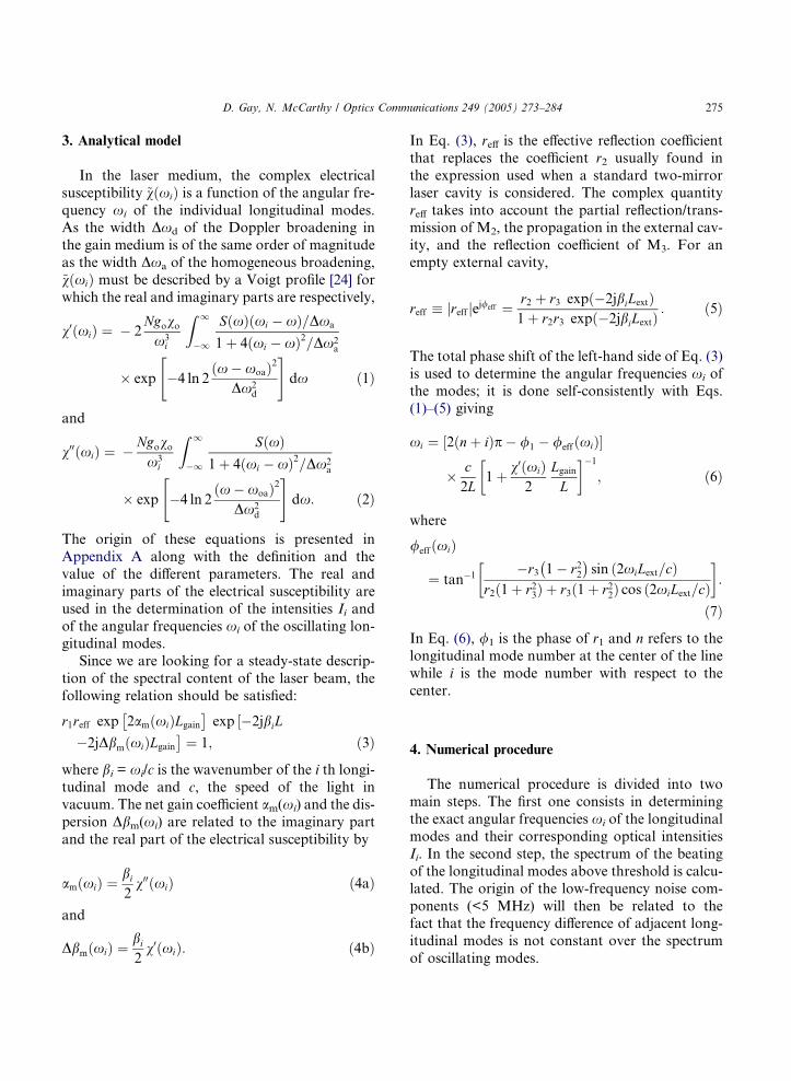
The total number of longitudinal modes con-

sidered in the calculations has been fixed to 91.

Fig. 3(a) shows the intensity spectral profile ob-tained after 10,000 roundtrips without external

cavity. Even if there were only 27 remaining

longitudinal modes, it was necessary to perform

calculations with so many modes in order to

completely saturate the gain. The spectral distri-

bution exhibits side modes with a relatively high

intensity due to the partially homogeneous

broadening of the gain medium. Each modecompetes with 6–8 neighboring modes while the

modes located on the sides of the intensity spec-

trum have to compete with only three or four

modes. That explains, for example, the relative

importance of modes i = ±12 with respect to

modes i = ±9. It has been also necessary to take

into account the effect of spontaneous emission

to represent adequately the evolution of the sat-uration of the gain medium. The spontaneous

emission was added at each roundtrip; its inten-

sity corresponds to one photon per mode per

half-life duration in the laser cavity. At

koa = 514.5 nm and for a loss coefficient of

0.0143 m�1, the intensity of the spontaneous

emission added at each roundtrip was about

10�6 W/m2.The numerical model includes a dispersion

term generated by the gain medium through

the Kramers–Kronig relations. Its effect on the

10-4

10-3

10-2

10-1

100

-50 -25 0 25 50

Inte

nsity

[MW

/m2 ]

mode number

(a)

10-3

10-2

10-1

100

101

1.349 1.35 1.351 1.352

Inte

nsity

(a.

u.)

frequency (GHz)

(b)

Fig. 3. (a) Calculated intensity of oscillating longitudinal

modes without feedback after numerical convergence and (b)

corresponding substructure of the 11th beat note of the

oscillating longitudinal modes.

10-4

10-3

10-2

10-1

100

101

-50 -25 0 25 50In

tens

ity [M

W/m

2 ]mode number

(a)∆L = 0.0 cm

10-4

10-3

10-2

10-1

100

101

-50 -25 0 25 50

Inte

nsity

[MW

/m2 ]

mode number

(b)∆L = -5.0 cm

10-4

10-3

10-2

10-1

100

101

-50 -25 0 25 50mode number

(c)

∆L = -10.7 cm

Inte

nsity

[MW

/m2 ]

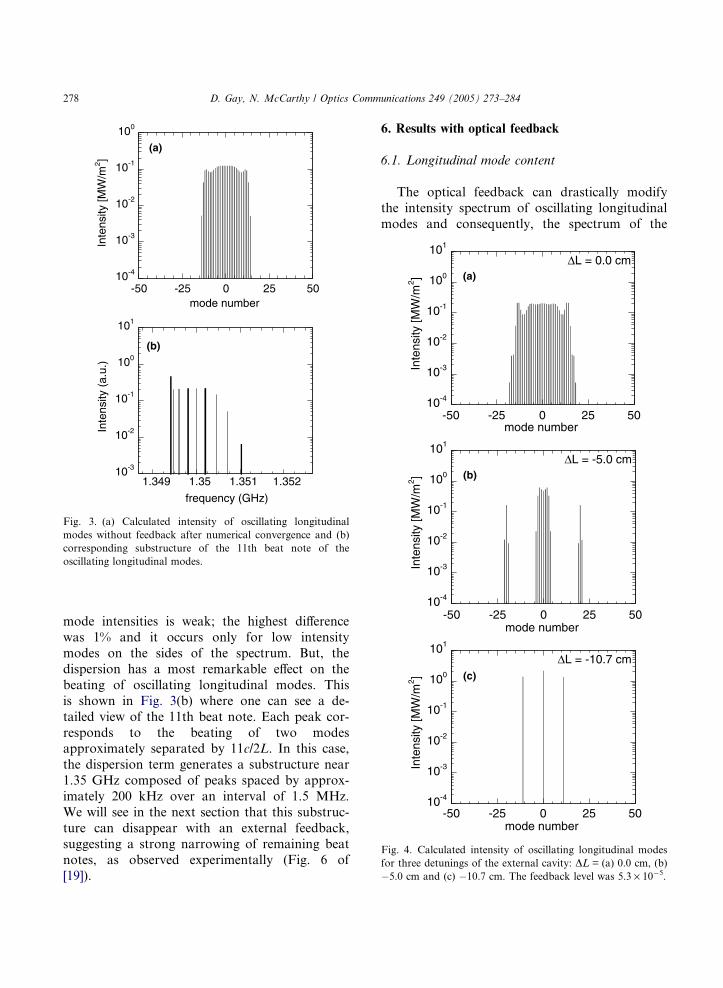
Fig. 4. Calculated intensity of oscillating longitudinal modes

for three detunings of the external cavity: DL = (a) 0.0 cm, (b)

�5.0 cm and (c) �10.7 cm. The feedback level was 5.3 · 10�5.


mode intensities is weak; the highest difference

was 1% and it occurs only for low intensity

modes on the sides of the spectrum. But, the

dispersion has a most remarkable effect on the

beating of oscillating longitudinal modes. This

is shown in Fig. 3(b) where one can see a de-

tailed view of the 11th beat note. Each peak cor-

responds to the beating of two modesapproximately separated by 11c/2L. In this case,

the dispersion term generates a substructure near

1.35 GHz composed of peaks spaced by approx-

imately 200 kHz over an interval of 1.5 MHz.

We will see in the next section that this substruc-

ture can disappear with an external feedback,

suggesting a strong narrowing of remaining beat

notes, as observed experimentally (Fig. 6 of[19]).

6. Results with optical feedback

6.1. Longitudinal mode content

The optical feedback can drastically modifythe intensity spectrum of oscillating longitudinal

modes and consequently, the spectrum of the

10-3

10-2

10-1

100

101

102

0 10 20 30 40 50

Inte

nsity

(a.

u.)

beat notes

(a) ∆L = 0.0 cm

10-3

10-2

10-1

100

101

102

0 10 20 30 40 50

Inte

nsity

(a.

u.)

beat notes

(b) ∆L = -5.0 cm

10-3

10-2

10-1

100

101

102

0 10 20 30 40 50

Inte

nsity

(a.

u.)

beat notes

(c) ∆L = -10.7 cm

10-3

10-2

10-1

100

101

1.349 1.35 1.351 1.352

Inte

nsity

(a.

u.)

frequency (GHz)

(d)11th beat note

Fig. 5. (a)–(c) Calculated beat notes corresponding to the spectra of Fig. 4. (d) Zoom of the 11th beat note shown in (c) using the same

scales as in Fig. 3 (b).


beat notes. Fig. 4 shows intensity spectra for

three different detunings DL(= Lext � L) of the

external cavity and Fig. 5 shows the correspond-

ing beat spectra. The feedback was set at

5.3 · 10�5; that was the experimental value pro-viding the best reduction of the low-frequency

noise components as shown later. For DL = 0

(Fig. 4(a)), the spectrum is nearly identical to

that calculated without feedback (see Fig. 3(a)).

The same statement is made when we compare

the beat spectrum of Fig. 5(a) to that obtained

without feedback (not shown). In that case,

the feedback does not reduce the number of lon-gitudinal modes but only slightly reduces the

losses of the laser cavity. However, for other

external cavity lengths, many modes are reduced

in intensity or eliminated (see Fig. 4(b) and (c)).

This behavior has been observed experimentally,

as reported in Figs. 7 and 8 of [19]. One may

also notice that a smaller number of remaining

modes produces an increase of their intensities.

For DL = �10.7 cm, only three modes have

survived (Fig. 4(c)) resulting in the presence of

only two strong beat notes in Fig. 5(c). The

effect of the feedback on the mode intensity

spectra is found to be symmetrical with respectto DL = 0. We observed both experimentally

and numerically that the strongest beat note

numbers, occurring when Lext is close to L, are

multiples of L/|DL|; this can be explained by

the periodicity of reff. The same behavior occurs

for Lext around 2L, as it has been observed

experimentally. The numerical simulations (and

the experiments) have also shown that the effectsobserved when the external mirror is located

near the output coupler M2 are very similar to

those obtained for L � Lext; the spectrum ob-

tained for DL = ±11 cm is identical to the one

obtained for DL = �111 cm (Lext = 11 cm).

However, for very short external cavities, the

strongest beat note numbers are rather multi-

ples of L/Lext. Finally, Fig. 5(d) shows a zoom

103

104

105

-15 -10 -5 0 5 10 15

Nor

mal

ized

sum

of b

eat n

otes

∆L (cm)

(a)

a

b

c

100

101

102

-15 -10 -5 0 5 10 15

Sen

sitiv

ity to

δL ex

t

∆L (cm)

(b)

Fig. 7. (a) Normalized sum of beat intensities as a function of

DL, for a feedback of 5.3 · 10�5. The black circles refer to the

cases illustrated in Figs. 4 and 5. (b) Sensitivity of the sum of

beat intensities to a small detuning of Lext as a function of DL.Each data was averaged with its 12 closest neighbors to bring

out the general behavior.


of the strong 11th beat note of Fig. 5(c). We

clearly see that the feedback can eliminate the

substructure of the remaining beat notes; exper-

imentally, a narrowing of them has also been

observed.

6.2. Noise reduction as a function of DL

By performing a sum on the beat note intensi-

ties, it is possible to roughly reproduce the

measured reduction of the low-frequency noise

components as a function of DL (experimental re-

sults recalled in Fig. 6). The sum is normalized tothe laser output power (which also depends on DL)and is shown in Fig. 7(a) for a feedback level of

5.3 · 10�5; the points a, b, and c on the graph refer

to the case of Figs. 4 and 5. One can see that this

calculation alone is not sufficient to explain the in-

crease of the noise components in the interval 1

cm < |DL| < 5 cm observed experimentally. In or-

der to reproduce more adequately this behavior,we have also simulated the effect of mechanical

vibrations of the external cavity and of the fluctu-

ations of the discharge (gain level) in the gain med-

ium, for the interval �15 cm < DL < 15 cm. We

assumed that mechanical vibrations cause a fluctu-

ation of 100 lm on the length of the external cav-

ity. Fig. 7(b) was obtained from the local average

of the subtraction of the data of Fig. 7(a) to thedata calculated with a small variation dL of 100

lm on Lext. The averaged sensitivity is shown to

-10

0

10

-15 -10 -5 0 5 10 15∆L (cm)

Rel

ativ

e no

ise

leve

l (dB

)

7 cm

7 cm

7 cm

7 cm

Fig. 6. Experimental measurements of the relative noise level

(averaged between 0 and 100 kHz) as a function of DL with a

feedback of 4 · 10�5. The shaded areas correspond to noise

reduction.

be lower for |DL| > 5 cm. On the other hand, it

reveals an increase of the sensitivity to dL in the

interval 1 cm < |DL| < 5 cm which indicates that

the relative mechanical vibrations of the cavities

may contributes to the low-frequency noise com-

ponents, as observed experimentally. Each curve

in Fig. 7 contains 500 calculated points, therefore,

the smooth aspect in some regions cannot be con-sidered as an artefact. Finally, we have simulated

the effect of the gain level fluctuations by assuming

a variation of the reflectivity dr1 of the rear mirror

M1. The variation was set to 10�4 generating a cal-

culated fluctuation of the output power of 7% (not

shown) as observed experimentally (see Fig. 2 of

[17]). Once again, the averaged sensitivity of the

sum of beat intensities to dr1 tends to be lowerfor |DL| > 5 cm which could add a contribution

to the relative noise level reduction in the interval

5 cm < |DL| < 12 cm (Fig. 6).

103

104

105

10-7 10-6 10-5 10-4 10-3 10-2

Nor

mal

ized

sum

of b

eat n

otes

Feedback level

∆L = -7.0 cm

a

b

c

Fig. 9. Normalized sum of beat note intensities as a function of

the feedback level for DL = �7 cm. The black circles refer to the

cases illustrated in Figs. 10 and 11.


6.3. Noise reduction as a function of the feedback

level

In this part, we show that the reduction of the

low-frequency noise components as a function ofthe feedback level (Fig. 8 displays the experimen-

tal results) can be reproduced numerically. The

detuning of the external cavity DL was set to �7

cm (the optimum value as shown in Fig. 6) and

the feedback level was varied from 10�7 to 10�3.

The experimental results exhibits a maximal noise

reduction close to a feedback of 5 · 10�5. The in-

crease of the feedback is equivalent to lower lossesand results in higher intracavity power. Thus, in

the numerical simulations, the sum of the beat

note intensities had to be normalized with respect

to the latter. Fig. 9 shows the normalized sum as a

function of the feedback level for DL = �7 cm.

Contrary to the intracavity power, the sum of beat

notes does not evolve monotonically with the feed-

back increase. There is an interval of feedbacklevel (close to 10�4) that minimizes the sum of beat

notes.

The observation of the calculated intensity spec-

tra of longitudinal modes has shown that a very

small feedback digs two small depressions in the

longitudinal mode spectra (see Fig. 10(a)). In that

case, the beat note distribution (Fig. 11(a)) is sim-

ilar to that obtained without feedback (Fig. 5(a)).As the feedback increases, these depressions get

-10

-5

0

5

10

10-7 10-6 10-5 10-4 10-3 10-2

Rel

ativ

e no

ise

leve

l (dB

)

Feedback level

Fig. 8. Relative noise level (averaged between 0 and 100 kHz)

as a function of the feedback level for DL = �7 cm: exper-

imental results.

deeper. For feedback higher than 2 · 10�6, the to-

tal power is shared between three clusters of longi-

tudinal modes. The narrowest clusters are

obtained for a feedback of 1.5 · 10�4 (Fig.

10(b)). In the beat note spectrum (Fig. 11(b)), only

few notes remain for this feedback; this situation

corresponds to the minimum of the curve in Fig.9(b). For feedback level further increased (Fig.

10(c)), mode groups get asymmetrical, more longi-

tudinal modes oscillate and more beat notes are

generated (Fig. 11(c)).

When we compare the experimental results

(Fig. 8) with the numerical ones (Fig. 9), we

clearly see that the same behavior, that is, the

feedback level can be optimized to reduce thelow-frequency noise components. But there is a

discrepancy on the optimum value of the feed-

back. Thus, numerical simulations have been car-

ried on to take into account the effect of

mechanical vibrations and of gain level fluctua-

tions. The sensitivity of the sum of beat notes

to fluctuations of DL and of r1 has been numeri-

cally evaluated for DL = �7 cm; results areshown in Fig. 12. Both curves exhibit a minimal

sensitivity for feedback between 6 · 10�5 and

1.2 · 10�4. These results suggest that those fluctu-

ations create a shift of the optimum feedback (see

Fig. 9) towards lower values, allowing conse-

quently a very good mapping with the experimen-

tal curve of Fig. 8.

10-3

10-2

10-1

100

101

102

0 10 20 30 40 50

Inte

nsity

(a.

u.)

beat notes

(a) 2.2x10-7

10-3

10-2

10-1

100

101

102

0 10 20 30 40 50

Inte

nsity

(a.

u.)

beat notes

(b) 1.5x10-4

10-3

10-2

10-1

100

101

102

0 10 20 30 40 50

Inte

nsity

(a.

u.)

beat notes

(c) 2.0x10-3

Fig. 11. Calculated beat notes corresponding to the spectra of

Fig. 10.

10-3

10-2

10-1

100

101

102

-50 -25 0 25 50

Inte

nsity

[MW

/m2 ]

mode number

(a)2.2x10-7

10-3

10-2

10-1

100

101

102

-50 -25 0 25 50

Inte

nsity

[MW

/m2 ] (b)

1.5x10-4

mode number

10-3

10-2

10-1

100

101

102

-50 -25 0 25 50

Inte

nsity

[MW

/m2 ]

mode number

(c) 2.0x10-3

Fig. 10. Calculated intensity of oscillating longitudinal modes

for three feedback levels: (a) 2.2 · 10�7, (b) 1.5 · 10�4, and (c)

2.0 · 10�3. The cavity detuning was DL = �7 cm.


7. Discussion

We have developed a model to describe the

behavior of the optical intensity noise in a cw ar-

gon ion laser coupled or not to an external empty

cavity. The partially inhomogeneous and homoge-neous nature of the broadening of the gain med-

ium has been included to better describe the

noise reduction. This model has been elaborated

in the spectral domain since the addition of the

external cavity implies an equivalent coupler

reflectivity that is function of the individual modefrequencies and thus modifies the distribution of

the power between the longitudinal laser modes.

The treatment in the spectral domain was justified

by the experimentally observed symmetry of the

reduction of the low-frequency noise components

as well as of the mode spectrum with respect to

100

101

102

10-7 10-6 10-5 10-4 10-3 10-2

Sen

sitiv

ity to

L ex

t

Feedback level

(a)

101

102

103

10-7 10-6 10-5 10-4 10-3 10-2

Sen

sitiv

ity to

δδ

r 1

Feedback level

(b)

Fig. 12. Sensitivity of the sum of beat intensities to a small

variation of (a) Lext and of (b) r1, as a function of the feedback

level.


Lext = L. Since the noise reduction is a function of

|DL| , it is not explained by a temporal effect as it

rather can be in mode-locked lasers [14].

The noise reduction, as observed experimentally

in three different intervals of frequencies and re-

ported in [19], has been reproduced by numerical

simulations. First, a large diminution of longitudi-

nal mode number caused by the filtering effect ofan external cavity with the appropriate length

and feedback has been obtained. Consequently,

it affected the calculated spectra of the notes, in

the hundreds of MHz (�nc/2L), generated by the

beating of oscillating longitudinal modes as we

observed experimentally. The low-frequency noise

level (<5 MHz) has been found to behave similarly

to the sum of the beating note intensities accordingto the experimental and simulated data as well as a

function of the external cavity length and of the

feedback level. This confirms that the low-

frequency noise in a cw argon ion laser originates

from a crossed-phase modulation phenomenon

between the beat notes and the population inver-

sion of the gain medium.

For some particular |DL| and reff, the few

remaining longitudinal modes are clustered; the

dispersion has then less effect on the widening ofthe beating notes. For example in Fig. 3(b), the

addition of an external cavity with DL = �10.7

cm and a feedback of 5.3 · 10�5 has reduced the

number of notes to only one component at 1.35

GHz (Fig. 5(d)). This has also been observed

experimentally as shown in Fig. 6 of [19].

Acknowledgments

This workwas supported by grants fromNatural

Sciences and Engineering Research Council

(Canada), the Fonds pour la Formation de Cherch-

eurs et l�Aide a la Recherche (Quebec), and the

Canadian Institute for Photonic Innovations CIPI

(Canada).

Appendix A. Electrical susceptibility of the argon

ion laser

In the expression of the electrical susceptibility~vðxiÞ of mode i, the Voigt profile comes from the

product of the Gaussian Doppler broadeninggd(x) of width Dxd and the Lorentzian lineshape~vh of width Dxa describing the homogeneous

broadening as formulated in the following integral

which also includes the saturation factor S(x) andthe density N of the population inversion [24]:

~v xið Þ ¼ NZ 1

�1gd xð ÞS xð Þ~vh xi; xð Þ dx; ðA:1Þ

where

gd xð Þ ¼ go exp �4 ln 2x� xoa

Dxd

� �2" #

; ðA:2Þ

~vh xi; xð Þ ¼ �jvox3

i

1

1þ 2j xi � xð Þ=Dxa

ðA:3Þ

and

S xð Þ ¼ 1þXi

I i=I sat1þ 2 xi � xð Þ=Dxa½ �2

( )�1

ðA:4Þ


with

go ¼1

Dxd

ffiffiffiffiffiffiffiffiffiffiffi4 ln 2

p

rðA:5Þ

and

vo ¼2pc3cradDxa

: ðA:6Þ

The frequency xoa is the center of the laser line

and corresponds to the wavelength koa (=514.5

nm). The full width at half maximum of Eq.

(A.2) is given by

Dxd ¼2pkoa

ffiffiffiffiffiffiffiffiffiffiffiffiffiffiffiffiffiffiffi8 ln 2kBT

M

r; ðA:7Þ

where kB is the Boltzmann constant and M, theatomic mass. The longitudinal temperature T of

ions has been determined from an extrapolation

of the curves (T versus discharge current) reported

in [25,26]. For a discharge current maintained be-

tween 20 and 30 A, the temperature is approxi-

mated to 5000 K and

Dxd ¼ 2p� 4:65 ½GHz�: ðA:8ÞThe width of the homogeneous broadening is

related to the decay rates s1 and s2 of the two levels

of the laser transition and to the dephasing time

due to collisional effects represented by a correc-

tion factor d [26]

Dxa ¼1

s1þ 1

s2

� �1þ dð Þ: ðA:9Þ

From [24–27], we found s1 = 3.5 · 10�10 s,

s2 = 6.2 · 10�9 s and d = 0.67 for discharge cur-rents between 20 and 30 A, giving

Dxa ¼ 2p� 0:8016� 109 ½rad=s�: ðA:10ÞThe radiative transition rate crad was considered

equal to 9.17 · 106 s�1 [27]. In Eq. (A.4), Ii is the

intensity of each longitudinal mode and Isat, the

saturation intensity

I sat ¼2phc s1 þ s2ð Þk3oacrads1s2 seffð Þ

1þ dð Þ

ffi 4:6� 105 1þ dð Þ ½W=m2�;ðA:11Þ

where seff = s1 + s2 � s1s2crad and h is the Planckconstant.

References

[1] P. Beaud, J.Q. Bi, W. Hodel, H.P. Weber, Opt. Commun.

80 (1990) 31.

[2] J.Q. Bi, W. Hodel, H.P. Weber, Opt. Commun. 81 (1991)

408.

[3] D. Cotter, Opt. Commun. 83 (1991) 76.

[4] J.Q. Bi, W. Hodel, H.P. Weber, Opt. Commun. 89 (1992)

240.

[5] H. Ammann, W. Hodel, H.P. Weber, Opt. Commun. 95

(1993) 345.

[6] N.I. Michailov, M. Chamel, Opt. Quant. Electron. 28

(1996) 653.

[7] D.S. Peter, P. Beaud, W. Hodel, H.P. Weber, Opt. Lett. 16

(1991) 405.

[8] P. Langlois, D. Gay, N. McCarthy, M. Piche, Opt. Lett.

23 (1998) 114.

[9] D. Gay, N. McCarthy, Opt. Commun. 137 (1996) 83.

[10] K. Mollmann, W. Gellermann, Opt. Lett. 19 (1994)

490.

[11] C.J.B. Riviere, R. Baribault, D. Gay, N. McCarthy, M.

Piche, Opt. Commun. 161 (1999) 31.

[12] N. McCarthy, S. Mailhot, J.-F. Cormier, Opt. Commun.

88 (1992) 403.

[13] J.M. Catherall, G.H.C. New, IEEE J. Quant. Electron. 22

(1986) 1593.

[14] G.H.C. New, Opt. Lett. 15 (1990) 1306.

[15] Y.A. Rzhanov, J.V. Moloney, Opt. Quant. Electron. 25

(1993) 63.

[16] M.C. Nuss, U. Keller, G.T. Harvey, M.S. Heutmaker,

P.R. Smith, Opt. Lett. 15 (1990) 1026.

[17] N. McCarthy, D. Gay, Opt. Lett. 16 (1991) 1004.

[18] S. Mailhot, N. McCarthy, Can. J. Phys. 71 (1993)

429.

[19] D. Gay, N. McCarthy, Opt. Commun. 193 (2001)

197.

[20] P. Besnard, F. Robert, M.L. Chares, G.M. Stephan, Phys.

Rev. A 56 (1997) 3191.

[21] P. Besnard, M.L. Chares, G. Stephan, F. Robert, J. Opt.

Soc. Am. B 16 (1999) 1059.

[22] A. Mihaescu, T.T. Tam, P. Besnard, G.M. Stephan, J.

Opt. B: Quant. Semiclass. Opt. 4 (2002) 67.

[23] J.-F. Lemieux, A. Bellemare, C. Latrasse, M. Tetu,

Electron. Lett. 35 (1999) 904.

[24] A.E. Siegman, Lasers, University Science Books, Mill

Valley, 1986, pp. 1292.

[25] M.H. Dunn, J.N. Ross, Prog. Quant. Electron. 4 (1976)

233.

[26] R.C. Sze, W.R. Bennett Jr., Phys. Rev. A: Gen. Phys. 5

(1972) 837.

[27] R.I. Rudko, C.L. Tang, J. Appl. Phys. 38 (1967) 4731,

Erratum: J. Appl. Phys. 39 (1968) 4046.

Modal content and noise characteristics of a cw argon ion laser with an optical feedback: Numerical...

Documents

Transcript of Modal content and noise characteristics of a cw argon ion laser with an optical feedback: Numerical...