Mod

Superv

Aug 20

K

dular Hy

visor: Jam

012

KTH School oEnDiv

ybridiz

Fo

mes Spellin

Masteroof Industriaergy Technvision of ApSE-100 4

zation o

or Deve

Ma

Maz

ng

fScienceTal Engineeriology EGI-2pplied heat a44 STOCKH

of Solar

eloping

aster Th

Of

zen Dar

Thesisng and Man2012-0823and powerOLM

Therm

Nation

hesis

rwish

nagement

mal Pow

ns

wer Plan

nts

Acknowledgment

I own the sincerest thanks to my thesis supervisor James Spelling, his continuous support and the time

he dedicated for this project has been an immense help, I would also like to thank my family that have

supported me throughout my two years of Masters studies in Sweden.

I would like also to express my gratitude for my friends who supported me personally and technically

and for the friendly and good times we have spent together throughout this period.

Abstract

The current energy scenario in the developing nations with abundant sun resource (e.g. southern

Mediterranean countries of Europe, Middle-East & North Africa) relies mainly on fossil fuels to supply

the increasing energy demand. Although this long adopted pattern ensures electricity availability on

demand at all times through the least cost proven technology, it is highly unsustainable due to its drastic

impacts on depletion of resources, environmental emissions and electricity prices. Solar thermal Hybrid

power plants among all other renewable energy technologies have the potential of replacing the central

utility model of conventional power plants, the understood integration of solar thermal technologies into

existing conventional power plants shows the opportunity of combining low cost reliable power and

Carbon emission reduction.

A literature review on the current concentrating solar power (CSP) technologies and their suitability for

integration into conventional power cycles was concluded, the best option was found be in the so called

Integrated solar combined cycle systems (ISCCS); the plant is built and operated like a normal combined

cycle, with a solar circuit consisting of central tower receiver and heliostat field adding heat to the

bottoming Rankine cycle.

A complete model of the cycle was developed in TRNSYS simulation software and Matlab environment,

yearly satellite solar insolation data was used to study the effect of integrating solar power to the cycle

throw-out the year. A multi objective thermo economic optimization analysis was conducted in order to

identify a set of optimum design options. The optimization has shown that the efficiency of the

combined cycle can be increased resulting in a Levelized electricity cost in the range of 10 -14 USDcts

/Kwhe. The limit of annual solar share realized was found to be around 7 %

The results of the study indicate that ISCCS offers advantages of higher efficiency, low cost reliable

power and on the same time sends a green message by reducing the environmental impacts in our

existing power plant systems.

1

CONTENTS

List of Figures 4

List of Tables 6

Nomenclature 7

1  Introduction ............................................................................................................................................... 9 

1.1  Objectives ......................................................................................................................................... 10 

1.2  Approach .......................................................................................................................................... 10 

2  Background .............................................................................................................................................. 11 

2.1  Solar Radiation ................................................................................................................................. 11 

2.2  Concentration of Solar Radiation ................................................................................................. 12 

2.3  Power conversion cycles ................................................................................................................ 14 

2.3.1  Rankine power generation cycle ........................................................................................... 15 

2.3.2  Brayton power generation cycle ............................................................................................ 16 

2.4  Over View of Concentrating Solar Power Technologies .......................................................... 17 

2.4.1  Parabolic Trough (Line focus, Mobile receiver) ................................................................. 17 

2.4.2  Linear Fresnel (Line focus, fixed receiver) .......................................................................... 18 

2.4.3  Tower power systems (Point focus, fixed receiver) ........................................................... 20 

2.4.4  Dish engine (Point focus, mobile receiver) ......................................................................... 23 

2.4.5  Comparison and Development Status ................................................................................. 24 

2.5  Integration options: ......................................................................................................................... 29 

2.5.1  Water / steam tower in a natural gas fired Combined cycle ( High temperature) ........ 29 

2.5.2  Atmospheric solar tower in natural gas fired Combined cycle ( High temperature) .... 30 

3  Power cycle model .................................................................................................................................. 30 

3.1  Introduction ..................................................................................................................................... 30 

3.2  The simulation software trnsys ..................................................................................................... 31 

3.3  Component models ......................................................................................................................... 33 

3.3.1  The heliostat field ................................................................................................................... 33 

3.3.2  The Tower ................................................................................................................................ 36 

3.3.3  The receiver ............................................................................................................................. 38 

2

3.3.4  The gas turbine ........................................................................................................................ 40 

3.3.5  Flow Mixer ............................................................................................................................... 42 

3.3.6  The heat recovery steam generator ...................................................................................... 42 

3.3.7  The steam turbine ................................................................................................................... 45 

3.3.8  The condenser ......................................................................................................................... 46 

3.3.9  Pumps ....................................................................................................................................... 46 

3.3.10  Open Feedwater heater (Deaerator)..................................................................................... 47 

3.3.11  Closed Feedwater heater ........................................................................................................ 47 

3.3.12  Other components .................................................................................................................. 48 

4  Economic analysis .................................................................................................................................. 49 

4.1  Cost functions .................................................................................................................................. 53 

4.2  Cost function of the gas turbine cycle .......................................................................................... 53 

4.2.1  Compressor .............................................................................................................................. 53 

4.2.2  Combustor ............................................................................................................................... 53 

4.2.3  Turbine unit ............................................................................................................................. 54 

4.2.4  Turbine auxiliaries ................................................................................................................... 54 

4.3  Cost functions for the steam cycle................................................................................................ 54 

4.3.1  HRSG ....................................................................................................................................... 54 

4.3.2  Steam turbine ........................................................................................................................... 55 

4.3.3  Turbine Auxiliaries.................................................................................................................. 56 

4.3.4  Pumps ....................................................................................................................................... 56 

4.3.5  Condenser and cooling tower ............................................................................................... 56 

4.4  Cost functions for the solar components .................................................................................... 57 

4.4.1  The heliostat field ................................................................................................................... 57 

4.4.2  Central tower ........................................................................................................................... 58 

4.4.3  Solar receiver ........................................................................................................................... 58 

4.4.4  Centrifugal Air Blower ........................................................................................................... 59 

4.5  Balance of plant costs ..................................................................................................................... 59 

4.5.1  Electrical generators ............................................................................................................... 59 

4.5.2  Civil engineering ...................................................................................................................... 59 

4.5.3  Natural Gas Substation .......................................................................................................... 60 

3

4.5.4  Contingencies and Decommissioning .................................................................................. 60 

4.6  Integrated solar combined cycle total investment ...................................................................... 61 

4.7  Operation and maintenance cost .................................................................................................. 61 

4.7.1  Fuel and water cost ................................................................................................................. 61 

4.7.2  Spare parts and repairs ........................................................................................................... 61 

4.7.3  Labour costs ............................................................................................................................ 62 

4.7.4  Service contracts ..................................................................................................................... 63 

4.8  Performance indicators .................................................................................................................. 63 

4.8.1  Solar share ................................................................................................................................ 63 

4.8.2  Carbon dioxide emissions ...................................................................................................... 63 

4.8.3  Power plant Fuel efficiency ................................................................................................... 64 

4.9  Data Transfer from Trnsys ............................................................................................................ 64 

5  Optimization of the integrated solar combined cycle ....................................................................... 65 

5.1  Multi-Objective Optimization ....................................................................................................... 65 

5.2  The optimization procedure .......................................................................................................... 68 

5.2.1  Thermoeconomic Objective functions ................................................................................ 69 

5.2.2  decision variables / Constants .............................................................................................. 69 

6  Optimization Results & Discussion ..................................................................................................... 70 

6.1  Effect of fuel cost increase ............................................................................................................ 79 

6.2  Effect of Heliostat Mirror Cost Reduction ................................................................................. 80 

7  Conclusions and Future work ............................................................................................................... 81 

8  Bibliography ............................................................................................................................................. 83 

4

List of Figures

Figure 1-1:The thesis flow chart .................................................................................................................... 10 Figure 2-1: Direct Normal Irradiance of the year 2002 in kWh/m²/y . .................................................. 12 Figure 2-2: Schematic of sun at Ts at distance R from a concentrator with aperture area. ................. 13 Figure 2-3 : Solar collector efficiency as a function of upper temperature for different concentration ratios and an ideal selective or a black body absorber . .............................................................................. 14 Figure 2-4: The ideal Carnot cycle ................................................................................................................. 14 Figure 2-5: Ideal Rankine cycle ..................................................................................................................... 15 Figure 2-6:Ideal Brayton Cycle ..................................................................................................................... 16 Figure 2-7: Parabolic trough collector field in Almeria Spain .................................................................. 18 Figure 2-8: Linear Fresnel test collector loop at the Plataforma Solar de Almería, Spain ................... 20 Figure 2-9: Solar tower power plant ............................................................................................................. 21 Figure 2-10: Dish-Sterling-System ................................................................................................................ 24 Figure 3-1: Plant process flow ....................................................................................................................... 30 Figure 3-2: information flow diagram for Gas turbine .............................................................................. 31 Figure 3-3: The Integrated Solar Combined Cycle in TRNSYS ............................................................... 32 Figure 3-4: Artist Illustration of a 46 MW plant ........................................................................................ 34 Figure 3-5: eSolar heliostat ............................................................................................................................ 35 Figure 3-6:Heliostat cleaning system ............................................................................................................ 35 Figure 3-7: The cosine effect for two heliostats in opposite directions from the tower. ..................... 36 Figure 3-8: Solar towers in California (Sierra commercial demonstration plant) .................................. 37 Figure 3-9: Open volumetric receiver principle and shape of hexagonal module cups of The Phoebus receiver . ............................................................................................................................................ 39 Figure 3-10: The SGT-800 ............................................................................................................................. 41 Figure 3-12: Energy/temperature diagram of a single-pressure HRSG .................................................. 42 Figure 3-11: Flow Mixer ................................................................................................................................. 42 Figure 3-13: Steam turbine stage ................................................................................................................... 45 Figure 3-14: Water cooled condenser ........................................................................................................... 46 Figure 3-15: open feedwater heater flow diagram ....................................................................................... 47 Figure 3-16: Temperature profiles for the feedwater heater. .................................................................... 48 Figure 4-1: Economic Indicators ................................................................................................................... 49 Figure 4-2: Estimated LCOE for new technologies ................................................................................... 51 Figure 4-3: NPV vs.Internal rate of return ................................................................................................. 52 Figure 5-1: Pareto optimal front ................................................................................................................... 66 Figure 5-2: Optimization data flow ............................................................................................................... 68 Figure 6-1: Typical POF curve ....................................................................................................................... 70 Figure 6-2: Annual solar share vs. Levelized cost of electricity ................................................................ 71 Figure 6-3 : Pareto optimal total mirror area vs. solar share ..................................................................... 72 

5

Figure 6-4: Live Steam pressure of Rankine cycle at 6 % solar share ...................................................... 73 Figure 6-5: Annual Solar share vs.NPV ........................................................................................................ 74 Figure 6-6: Annual solar share vs. Total equipment cost ........................................................................... 75 Figure 6-7: Specific CO2 emissions vs. solar share .................................................................................... 76 Figure 6-8: Selected design points on the POF ........................................................................................... 77 Figure 6-9 : Cost Breakdown for two design options, California Site ..................................................... 78 Figure 6-10 : Cost Breakdown for two design options, Palermo Site ...................................................... 78 Figure 6-11: Effect of natural gas price on LCOE ..................................................................................... 79 Figure 6-12: LCOE vs. solar share at different heliostat prices ................................................................ 80 

6

List of Tables

Table 2-1: Overview of main Technical Characteristics of CSP technologies ..................................... 26 Table 2-2: Overview of main commercial characteristics of CSP technologies ................................... 27 Table 2-3: Estimated current (2010) and future costs (2020) for parabolic Trough & Power Tower Systems. ............................................................................................................................................................. 29 Table 3-1: Single heliostat field charecteristics ............................................................................................ 34 Table 3-2: Correlation used for Nusselt number ....................................................................................... 38 Table 3-3: Insulation material properties .................................................................................................... 38 Table 3-4: Characteristics of receiver module material ............................................................................. 39 Table 3-5:Technical specifications for SGT-800 gas turbine .................................................................... 41 Table 3-6: HRSG design parameters ............................................................................................................. 43 Table 3-7: Effectiveness-NTU relations for different heat exchanger types ......................................... 45 Table 3-8: Condenser assumed values .......................................................................................................... 46 Table 4-1: Costs / Prices and economical settings .................................................................................... 50 Table 4-2: Infrastructure & building cost ..................................................................................................... 59 Table 4-3: Labour Rates (in USD/yr) and Plant Labour Requirements .................................................. 62 Table 5-1: Selected decision variable and ranges ......................................................................................... 69 Table 5-2: Selected constants and values ...................................................................................................... 69 Table 6-1: Selected point’s characteristics .................................................................................................... 77 

7

Nomenclature

Abbreviations

CSP Concentrated solar power

LCOE Levelized cost of electricity

NPV Net present value

DNI Direct normal irradiation

DLR Deutsches Zentrum Für Luft- und Raumfahrt (German Aerospace Center)

HTF Heat transfer fluid

PTC Parabolic trough collector

DSG Direct steam generation

LFR Linear Fresnel reflector

ISCC Integrated solar combined cycle

DOE US Department of energy

EIA International energy agency : check if eia or iea

HRSG Heat recovery steam generator.

STEC Solar thermal electric component library

NTU Number of transfer units

UA Overall heat transfer coefficient

CRF Capital recovery factor

M&S Marshall and Swift index

MMBTU One million British thermal units

MOO Multi objective optimizer

POF Pareto optimal front

EA Evolutionary algorithm

OSMOSE OptimiSation Multi Objectivs de Systemes Energetiques integers

8

Characters Symbols

A Surface Area [m2] α Absorptance [-] B Net Annual benefits [USD] ε Emmitance [-] c Concentration Ratio [-] σ Stefan Boltzman constant [W/m2k4] C Cost [USD] θs Acceptance Angle [Rad] cp Specific heat capacity [ J/KgK] ηc Carnot Efficiency [-] d Diameter [m] Є Porosity [-] Dh Hydraulic Diameter [m] μ Dynamic Viscosity [Kg/ms] DTPP Evaporator pinch point [-] Density [Kg/m3]

DTAP Economizer water approach [-] Mirror field reflectivity [-]

Cr Capacitance Heat ratio [-] ∏ Pressure ratio [-] E Produced Electricity [Kwh] f Friction factor [-] Indices fT Temperature correction factor [-] abs Absorber fη Efficiency correction factor [-] act Actual fM&S Marshal & Swift Index [-] aux Auxiliary Gsc Solar constant [W/m2] comb Combustion

Chamber Go Air mass velocity [Kg/m2s] cond Condenser h Specific enthalpy [J/Kg] cw Cooling water H Tower Height [m] eco Economizer IT Incident solar radiation [W/m2] elec Electric k Thermal conductivity [W/mk] evap Evaporator Kins Insurance rate [USD] fire Firing L Length [m] gen Generator m Mass [Kg] gt Gas Turbine N Number [-] helio Heliostats Nu Nusselt Number [-] ins Insurance p Pressure [Bar] inv Investment Pr Prandtl number [-] max Maximum P/Q Power [W] mec Mechanical Q Heat transfer [KJ] min Minimum R Sun earth mean distance [m] mir Mirror r Radius [m] opt Optical Re Reynolds number [-] rec Receiver T Temperature [K] ref Reference U Overall heat transfer coefficient [w/m2k] sat Saturated v Velocity [m/s] sh Superheater V Volumetric flow rate [m3/s] sol Solar W Work [ J] st Steam Turbine X Decision space [-] tec Technician

9

1 INTRODUCTION The current energy scenario in the developing nations with abundant sun resource (e.g. southern Mediterranean countries of Europe, Middle-East & North Africa) relies mainly on fossil fuels to supply the increasing energy demand. Although this long adopted pattern ensures electricity availability on demand at all times through the least cost proven technology, it is highly unsustainable due to its drastic impacts on depletion of resources, environmental emissions and electricity prices. Solar thermal Hybrid power plants among all other renewable energy technologies have the potential of replacing the central utility model of conventional power plants[1], the understood integration of solar thermal technologies into existing conventional power plants shows the opportunity of combining reliable power despicability without the added cost of thermal storage and Carbon emission reduction . The main barriers of up taking solar energy systems in developing countries are: the high initial investments of renewable only power plants especially at high capacities needed for developing countries in the upcoming future, fossil fuel subsidies especially to natural gas, which leads to misleading prices and impedes the development of renewable energy. One solution to overcome the initial cost barriers and to make use of lower price fossil fuel like natural gas is the deployment of modular hybrid solar thermal power plants; the concept is based on attaching a small solar field to a newly built conventional fossil fuel power plant with the power block designed to accommodate for increasing share of solar heat input over time by increasing the area of the solar field thus reducing the barrier of high initial investment and fuel escalation rates in the coming years. Several projects have been implemented where heat from solar energy is introduced into a combined cycle power plant (e.g. Hassi Rmel plant in Algeria and Ain Beni Mathar plant in Morocco)[2], up until now the only concentrating power technology considered for this type of plants is the parabolic trough collectors, this study will present an option for using different technology ( Central receiver tower systems) in the integrated solar combined cycle power plant.

10

1.1 OBJECTIVES The main objectives of this thesis can be summarized as follows:

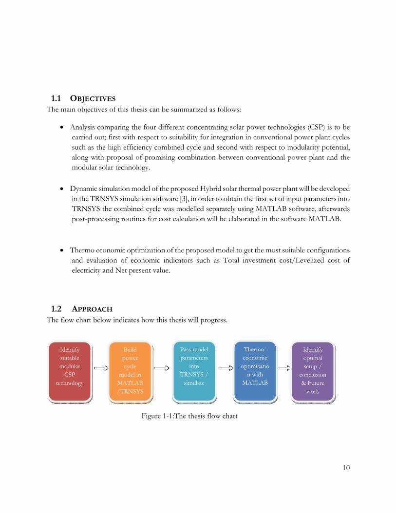
Analysis comparing the four different concentrating solar power technologies (CSP) is to be carried out; first with respect to suitability for integration in conventional power plant cycles such as the high efficiency combined cycle and second with respect to modularity potential, along with proposal of promising combination between conventional power plant and the modular solar technology.

Dynamic simulation model of the proposed Hybrid solar thermal power plant will be developed in the TRNSYS simulation software [3], in order to obtain the first set of input parameters into TRNSYS the combined cycle was modelled separately using MATLAB software, afterwards post-processing routines for cost calculation will be elaborated in the software MATLAB.

Thermo economic optimization of the proposed model to get the most suitable configurations and evaluation of economic indicators such as Total investment cost/Levelized cost of electricity and Net present value.

1.2 APPROACH The flow chart below indicates how this thesis will progress.

Identify suitable modular

CSP technology

Build power cycle

model in MATLAB /TRNSYS

Pass model parameters

into TRNSYS /

simulate

Thermo-economic

optimization with

MATLAB

Identify optimal setup /

conclusion& Future

work

Figure 1-1:The thesis flow chart

11

2 BACKGROUND In this chapter the basic concepts for concentrating solar energy engineering are explained, followed by an overview of concentrating power technologies. A comparison between the different concentrating technologies is viewed, finally, the integration issues between solar technologies and conventional power plant is explained and the option most suitable for this work is decided.

2.1 SOLAR RADIATION The solar radiation that reaches the earth’s surface radiates from the sun, continuous fusion reactions at the sun’s core result in temperatures between 8x106 to 40x106 Kelvin [4] , this heat is then transferred to the radiative surface of the sun (Photosphere) which has an effective black body temperature of around 5800 Kelvin. The rate of radiant energy incident upon a unit area of surface is called irradiance [W/m2], when irradiance is integrated over a specified period of time (e.g. day, hour) it becomes solar irradiation which has units of [Wh/m2]. Irradiation over a period of one complete day becomes solar insolation [kWh/m2/day].

The mean earth-sun distance is estimated at 1.49x1011 m; radiation emitted by the sun measured on the outside of the earth atmosphere results in a nearly constant flux density, and is called the solar constant:

GSC = 1367 [W/m2]

(2.1)

This amount varies by ±3% as the earth orbits around the sun[4], the amount of this flux density that reaches the earth surface is around 1000W/m2[5], this amount is affected by several factors; variation with the time of day and year, latitude variation and most important weather conditions affects the solar radiation reaching the earth’s surface.

Solar radiation consists generally of two main components; direct beam radiation is defined as the radiation received from the sun without being scattered by the atmosphere while the second component is the diffuse (scattered) radiation, the sum of the two components is the total solar radiation. In Concentrating solar power applications direct beam radiation is important since CSP systems can only collect this component, for this reason CSP systems are designed to track the sun during the day.

Solar irradiance is a crucial factor for CSP plant design, location and economics of the plant. Available solar data sources are ground level measurements and Meteorological satellite data. While ground measurements are more accurate than satellite data they are expensive with no possibility of delivering past data [6], the combination of both ground and satellite measurement yields accurate irradiation maps that can be used in planning and cost calculation of a solar power venture.

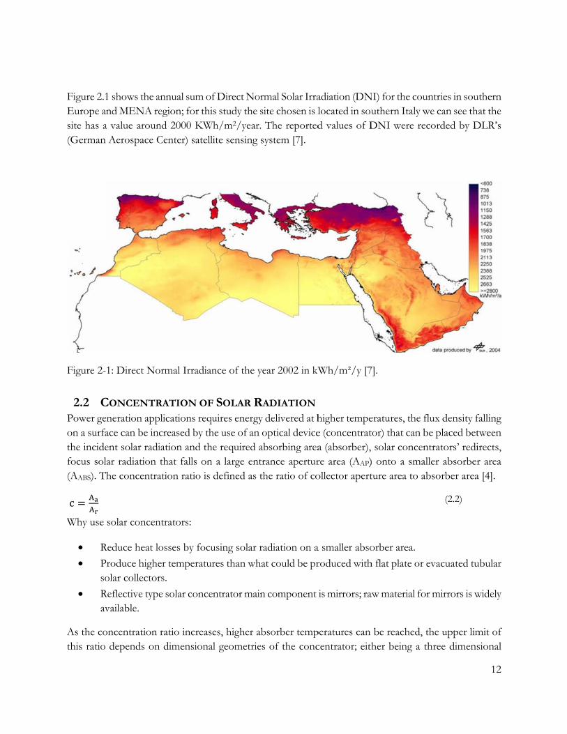
Figure 2.1Europe asite has a(German

Figure 2-

2.2 CPower geon a surfathe incidefocus sol(AABS). T c =

Why use

R

Pso

Rav

As the cothis ratio

1 shows the and MENA re

a value arounAerospace C

1: Direct No

CONCENTR

eneration appace can be incent solar radilar radiation he concentra

solar concen

Reduce heat lo

Produce higheolar collector

Reflective typevailable.

oncentration depends on

annual sum ofegion; for thind 2000 KWCenter) satell

ormal Irradian

RATION OF

plications requcreased by thiation and ththat falls on

ation ratio is

ntrators:

osses by focu

er temperaturrs.

e solar conce

ratio increasn dimensiona

f Direct Normis study the si

Wh/m2/year. Tlite sensing sy

nce of the ye

F SOLAR RA

uires energy he use of an ohe required ab

a large entrdefined as th

using solar ra

res than wha

entrator main

es, higher abal geometries

mal Solar Irraite chosen is lThe reportedystem [7].

ear 2002 in kW

ADIATION

delivered at hoptical devicebsorbing arearance aperturhe ratio of co

adiation on a

at could be pr

n component

bsorber temp of the conc

adiation (DNlocated in soud values of D

Wh/m²/y [7

higher tempee (concentrata (absorber), re area (AAP)ollector apert

a smaller abso

roduced with

is mirrors; ra

peratures can centrator; eith

NI) for the couuthern Italy wDNI were re

7].

eratures, the ftor) that can b solar concen) onto a smature area to a

orber area.

h flat plate or

aw material fo

be reached, her being a t

untries in souwe can see thecorded by D

flux density fbe placed betntrators’ redialler absorberabsorber area

(2.2)

evacuated tu

or mirrors is w

the upper limthree dimens

12

uthern hat the DLR’s

falling tween irects, r area a [4].

ubular

widely

mit of sional

(circular) aperture a

radius of

Figure 2-

Solar conreceiver tfocusing concentra

For a poiC =For two d

C =

The maxiupper limopaque flT ,Where: Ta : Amb

α: Absorpσ: Stefan ε : EmmiIT : IncideA A ⁄ :

concentratorarea AAP and

the sun. The

2: Schematic

ncentrators catowers, dish

systems (e.ated along a

int focus (circ= dimensional = 21imum theore

mit of concenlat surface tak= T + (∝bient tempera

ptance of abs

Boltzmann citance of the ent solar radiConcentratio

r or two-dimd absorber are

e angle subte

c of sun at Ts

an be classifiesystems) whg. parabolicfocal line.

cular concen45,000

(linear) conc2

etical temperantration ratioking into acc∝ ε)(⁄ I /σ)(ature.

sorber surfac

constant (5.6absorber suriation from ton ratio.

ensional (lineea AABS facin

nded by the

s at distance

ed by their fohere all solar c trough, lin

ntrator) the m

centrators the

ature that cano given by eqcount radiativ(A A )⁄ ⁄

ce.

67 x 10-8 W/mrface. the sun at 580

ear) concentrng the sun, R

sun (θS) appr

R from a con

cus geometryradiation can

near Fresnel

maximum pos

e maximum p

n be attainedquation 2.5. Tve heat losses

m2 K4).

00 K.

rator, Figure (is the sun-ea

roximately eq

ncentrator w

y; either as pon be concent

systems) w

ssible concen

possible conc

d is the sun’sThe maximums only and no

(2.2) shows a arth mean dis

quals 0.27 °

with aperture

oint focus systrated to a si

where solar

ntration ratio

centration ra

s temperaturem temperatuo heat extrac

concentratorstance where

[4].

area. [8]

stems (e.g. Cingle point oradiation ca

o is given by:

(2.3)

atio is given b

(2.4)

e of 5800 K ure achieved ction is given

(2.5)

13

r with e r the

entral or line an be

by:

at the by an

n by:

Figure (2the efficie(high Absa significathe achievdo not ex

Figure 2-ratios and

2.3 PHigh temconventioBrayton (Plants [9]

Thermal eshows thprocesses

T

.3) shows theency drops asorptance of ant gain in thved temperatxist and the e

3 : Solar colld an ideal sele

POWER CON

mperature solaonal power cy( gas turbine .

efficiency of he T_S diagras and two ise

TL

TH

T[K]

Figure

e solar collect higher temp

f wave lengthhe efficiency tures will be

efficiency var

ector efficienective or a bl

NVERSION

ar heat produycles describecycle). Curre

the two convam of a theo

entropic proc

S

1

2

e 2-4: The id

ctor efficiencyperatures due

hs in the solarcan be achievlower than th

riation due to

ncy as a funclack body ab

N CYCLES uced by conceed in the folloently the stea

ventional poworetical Carn

cesses.

S [J/kg]

3

deal Carnot cy

y increases ae to the increr spectrum anved especiallhe values sho

o fluctuation

ction of uppesorber [7].

entrating systowing sectionam turbine cy

wer cycles is lnot cycle wh

4

ycle

as concentratieased heat lond low emmly at lower coown due to tin solar radia

er temperatur

tems, is convns; the Rankinycles are the

limited by thehich consists

ion ratios incosses. For sel

mitance in theoncentration the fact that pation.

re for differe

verted to electne (steam turbmost used in

e Carnot efficof two reve

crease. Howeective absorb

e infrared regratios. In rea

perfect absor

ent concentra

tricity by usinbine) cycle ann commercial

ciency. Figureersible, isoth

14

ever bers

gion) ality rbers

ation

ng two nd the l CSP

e (2.4) ermal

Heat is aworking fcycle’s lowη =In order then rejecabsorber HoweverconcentraCSP pow

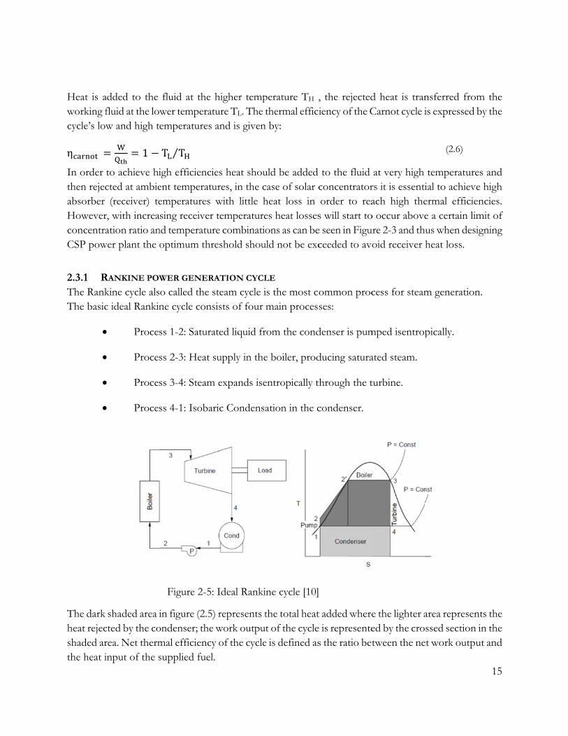
2.3.1 RThe RankThe basic

The dark heat rejecshaded arthe heat i

added to the fluid at the low and high t= = 1 −to achieve hicted at ambie(receiver) te

r, with increaation ratio an

wer plant the

RANKINE POW

kine cycle alsc ideal Rankin

Proce

Proce

Proce

Proce

shaded area icted by the corea. Net therminput of the s

fluid at the wer temperatemperatures T T⁄

igh efficiencient temperatuemperatures sing receiver

nd temperaturoptimum thr

WER GENER

o called the ne cycle cons

ss 1-2: Satura

ss 2-3: Heat

ss 3-4: Steam

ss 4-1: Isoba

Figure 2-5:

in figure (2.5)ondenser; themal efficiencysupplied fuel

higher tempture TL. The tand is given

ies heat shouures, in the cwith little h

r temperaturere combinatioreshold shou

RATION CYCL

steam cycle isists of four

ated liquid fr

supply in the

m expands ise

aric Condensa

: Ideal Ranki

) represents te work outpuy of the cyclel.

perature TH ,thermal effici

n by:

uld be added case of solar cheat loss in es heat lossesons as can be

uld not be exc

LE is the most comain proces

rom the cond

e boiler, prod

entropically t

ation in the c

ine cycle [10]

the total heatt of the cycle

e is defined as

, the rejectediency of the C

to the fluid concentratororder to rea

s will start toe seen in Figuceeded to av

ommon procses:

denser is pum

ducing satura

through the t

condenser.

t added wheree is representes the ratio bet

d heat is tranCarnot cycle i

at very high rs it is essentiach high the

o occur aboveure 2-3 and thoid receiver

cess for steam

mped isentrop

ated steam.

turbine.

e the lighter aed by the crotween the ne

nsferred fromis expressed b

(2.6)

temperatureial to achieveermal efficiee a certain limus when desiheat loss.

m generation

pically.

area represenssed section

et work outpu

15

m the by the

es and e high ncies. mit of igning

n.

nts the in the ut and

Thermal superheatimprovinsteam quafterwardOther moin one or

In commsuccessfumodelledtwo sourc

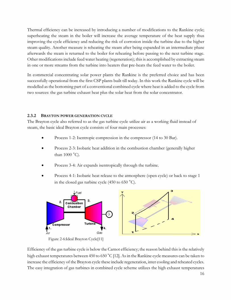
2.3.2 BThe Braysteam, th

Efficienc

high exhaincrease tThe easy

efficiency cating the stea

ng the cycle eality. Anothe

ds the steam odifications inmore stream

mercial conceully operationd as the bottomces: the gas t

BRAYTON PO

yton cycle alse basic ideal

Proce

Proce

than 1

Proce

Proce

in the

Figure 2-6

y of the gas tu

aust temperatthe efficiencyintegration o

an be increasam in the bofficiency and

er measure isis returned tnclude feed w

ms from the t

entrating solanal from the fming part of turbine exhau

OWER GENER

o referred toBrayton cycl

ss 1-2: Isentr

ss 2-3: Isoba

1000 °C).

ss 3-4: Air ex

ss 4-1: Isoba

closed gas tu

:Ideal Brayton

urbine cycle i

tures betweeny of the Braytof gas turbine

ed by introduoiler will incrd reducing th reheating th

to the boiler water heatingturbine into h

ar power plafirst CSP plana convention

ust heat plus

RATION CYCL

o as the gas tule consists of

ropic compre

aric heat addi

xpands isentr

aric heat relea

urbine cycle

n Cycle[11]

is below the C

n 450 to 650 °on cycle theses in combin

ucing a numrease the avehe risk of corhe steam afte

for reheatingg (regeneratioheaters that p

nts the Ranknts built till tonal combinedthe solar hea

LE urbine cycle uf four main p

ession in the

tion in the co

ropically thro

ase to the atm

(450 to 650 °

Carnot effici

°C [12]. As inse include regned cycle sch

mber of modierage temperrrosion insideer being expag before pas

on); this is accpre-heats the

kine is the poday. In this d cycle whereat from the s

utilize air as processes:

compressor

ombustion c

ough the turb

mosphere (op

°C).

iency; the rea

n the Rankinegeneration, ineme utilizes

fications to trature of thee the turbineanded in an inssing to the ncomplished be feed water t

preferred chowork the Ran

e heat is addedsolar concent

a working flu

(14 to 30 Ba

hamber (gen

bine.

pen cycle) or

son behind th

e cycle measuter cooling anthe high exh

the Rankine e heat supplye due to the hntermediate pnext turbine by extracting sto the boiler.

oice and has nkine cycle wd to the cycletrator.

uid instead o

ar).

nerally higher

back to stag

his is the rela

res can be taknd reheated c

haust tempera16

cycle; y thus higher phase stage. steam .

been will be e from

of

r

ge 1

atively

ken to cycles. atures

17

that provide heat input to the bottoming Rankine cycle leading to higher efficiency. In commercial CSP power plants today hybrid gas turbine solar cycle has only be tested on a small scale prototypes which is further discussed in section 2.4.3.4, in this work the gas turbine is introduced as a part of an integrated solar combined cycle power plant.

2.4 OVER VIEW OF CONCENTRATING SOLAR POWER TECHNOLOGIES

2.4.1 PARABOLIC TROUGH (LINE FOCUS, MOBILE RECEIVER)

Parabolic trough systems concentrate solar radiation by redirecting the incident rays parallel to the optical axis of a parabolic shaped reflector (mirror) onto a focus line which contains the receiver. Radiation is absorbed in the receiver and converted to another energy form [4] thus increasing the temperature of the circulating heat transfer fluid (HTF) inside the receiver. Parabolic trough power plants consist of many parallel rows of single axis-tracking concentrators and are modular in nature; they can be deployed at a wide range of capacities. For the current time the optimal capacity for trough plants is estimated to be 150-200 MW [1].

The receiver contains stainless steel pipes treated with selective coating that absorbs solar radiation while at the same time has very low infra-red radiation emmitance, the pipes are enclosed in evacuated glass tubes to minimize convective losses. The heat transfer fluid from the collector’s transfers’ heat in the heat exchangers where water is evaporated and high pressure super-heated steam expands through the turbine of a Rankine cycle, which drives a generator for electricity production. Steam is then cooled and condensed, after which water returns to the heat exchangers. Currently the maximum operating

temperature in most PTC plants is around 390°C and that is due to damage to the HTF which is mostly

synthetic oil if heated above 400 °C, the use of other heat transfer fluids such as molten salts or direct steam can help achieve higher temperatures as they have higher heat resilience than oil. The Archimede project developed by the Italian National Environmental & Renewable Research center (ENEA) is a 5 MW parabolic trough system using a mixture of nitrate salts as a HTF with solar field outlet temperature

up to 550 °C, the plant started production in July 2010.[13]. However the high freezing temperatures and the related investment costs pose a challenge to molten salts as a HTF. Direct Steam Generation (DSG) in parabolic trough holds advantages over the use of oil as a HTF [14]; the temperature of the HTF can be increased over the currently limited 400 C ͦ of oils and the overall costs of the plants are lower due to unnecessary oil/ steam heat exchanger. However, research is still going on DSG technology to solve potential problems relating to two phase flows and control systems. Parabolic trough is the most mature technology in large concentrating power schemes that is due to the experience gained from the success operation of the Solar Energy Generating Systems (SEGS) trough plants built in the Mohave Desert in California between 1984 and 1991. Current installed capacity of parabolic trough plants exceeds all other CSP technologies with large number of projects in the pipeline [15]

F

2.4.2 L Linear Frparabolica fixed reHTF and Linear Frgeneratiosteam genC ͦ (Saturbefore enfired heat

Figure 2-7: Pa

LINEAR FRES

resnel reflecto troughs, theceiver which

d mounted on

resnel plants n as a HTF,

neration systeated steam),

ntering the tuter or a boile

arabolic troug

SNEL (LINE

ors (LFR’s) c arrays of mir

h can be coupn a tower wit

can be operathis holds an

em is requiredthe produce

urbine , wet sr is placed pa

gh collector f

FOCUS, FIXE

onsists of flarrors are laid

pled with a seth a height ra

ated with oil n advantage d, operating sed steam is sesteam and coarallel to the

field in Alme

ED RECEIVE

at or slightly cclose to the gcondary refle

anging from

or molten saover parabolteam conditient afterwardondensed wasolar field to

eria Spain [16

ER)

curved mirrorground in lonector from ab10-15 meters

alts HTF fluilic trough plaons in Fresneds to a separater are circulo ensure desp

6]

rs which rougng rows to rebove the absos high [17].

ids but mainlants since noel plants are urator in orderlated throughpicability.

ghly approximflect sunlightorber contain

ly use direct so need of sepusually 50 barr to dry the sh the cycle . A

18

mates t onto ning a

steam parate r/ 270 steam A gas

19

Latest developments in Fresnel technology show that production of superheated steam is possible; in 2011 Novatec’s solar Fresnel collector in Spain successfully generated super-heated steam with temperatures above 500C ͦ [18]. The main advantages over parabolic troughs can be summarized as:

Cheap flat or slightly curved mirrors.

Fixed absorber tubes eliminating the need for flexible high pressure joints.

Low wind loads and reduced material used in the structure due to ground proximity.

Direct steam generation, eliminating the need for steam generators.

Low land use, developers like AREVA claim their Fresnel technology is the most land efficient in all CSP technologies.

Fresnel collector major drawback lies in higher optical losses of the fixed receiver compared to parabolic troughs , shading and blocking between the closely spaced mirrors reduced the efficiency and leads to increased spacing or receiver height. A new concept was developed to overcome the above mentioned problems, compact linear Fresnel collector (CLFR) technology [19]. In CLFR systems a large number of linear receivers on elevated tower structures that are close enough for individual mirror rows to have the option of directing the reflected solar rays to at least two alternative receivers on separate towers. This allows for more densely packed reflectors with less shading and blocking. Although LFR’s are less efficient than parabolic troughs in converting solar energy to electricity the low cost of the technology can bridge the gap making LFR’s a main competitor to parabolic troughs in the near future [20].

Figure 2-

2.4.3 T

Power towtwo-axis about 100

temperatuthe receivconventio Power topower codecades:

8: Linear Fre

TOWER POWE

wer systems tracking syst0 meters. Hel

ures from 800ver absorbs onal power c

ower plants aonversion cyc

esnel test coll

ER SYSTEMS

concentrate stems) to refleliostats can re

0 to over 100the solar en

cycle.

are often chacle. Four main

lector loop a

(POINT FOC

sunlight by uect sunlight oeach concent

00 °C. The recnergy convert

aracterized byn configurati

at the Platafo

CUS, FIXED R

sing a field oonto a receivtration ratios

ceiver collectting it into t

y the heat trions of tower

orma Solar de

RECEIVER)

f heliostats (lver on top of

between 300

s the heat andthermal ener

ransfer fluid,r systems hav

e Almería, Sp

large individuf a tower wit0-1500 suns,

d a HTF that rgy to produ

, thermal stove been studi

pain [16]

ual mirrors thth a height uachieving rec

circulates thruce electricity

orage mediumies in the last

20

hat use usually ceiver

rough y in a

m and three

W

M

A

P

2.4.3.1 W

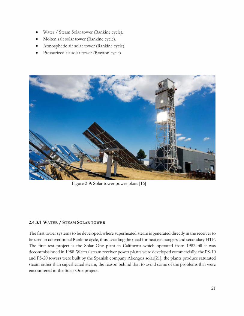
The first tbe used inThe firstdecommiand PS-20steam ratencounte

Water / Steam

Molten salt so

Atmospheric

Pressurized ai

WATER / STE

tower systemn convention

test projectissioned in 190 towers werher than sup

ered in the So

m Solar tower

olar tower (R

air solar tow

ir solar tower

Figure 2-9:

EAM SOLAR T

ms to be develnal Rankine cyt is the Sola988. Water/ sre built by theerheated stea

olar One proj

r (Rankine cy

ankine cycle)

er (Rankine c

r (Brayton cy

: Solar tower

TOWER

loped; whereycle, thus avoar One plantsteam receivee Spanish comam, the reasoject.

ycle).

).

cycle).

ycle).

r power plant

superheated oiding the neet in Californer power planmpany Aben

on behind tha

t [16]

steam is geneed for heat exnia which opnts were devengoa solar[21at to avoid so

erated directlxchangers anperated fromeloped comm], the plants

ome of the p

ly in the receivnd secondary m 1982 till imercially; the P

produce saturoblems that

21

ver to HTF. t was PS-10 urated t were

22

2.4.3.2 MOLTEN SALT SOLAR TOWER Molten salt mixtures offers excellent performance as heat transfer fluids in advanced power plant concepts, the best mixture was found to be 60 % sodium nitrate / 40 % potassium nitrate[22]. The main benefits of molten salts as HTF’s are the excellent heat transfer properties and lower pressure, high temperature energy storage in another important advantage thus increasing the capacity factor of the plant , salts can be stored in large tanks at atmospheric pressure to be used when the sun is not shining or at nights. Disadvantages of using salts as a HTF lies in the high freezing temperatures (120 to 220 C ͦ ) and the increased operational and maintenance costs related to freeze protection, piping and fitting materials. In a molten salt tower plant, salt mixture enters the receiver at 290 C ͦ and exists around 565 C ͦ, the hot salt is then pumped to the steam generator producing superheated steam to be used for electricity production in a conventional Rankine cycle[22]. The first test facility to demonstrate molten salt tower technology as a commercial technology was the Solar Two project in California.

2.4.3.3 ATMOSPHERIC AIR SOLAR TOWER Another concept is Central receiver solar power plants working with atmospheric air as a HTF based on the PHOEBUS scheme [23]; a blower circulates air through the receiver consisting of metallic or ceramic materials on top of the tower, which is heated by the concentrated sunlight to temperatures

between 650 and 850 °C afterwards the hot air is used to produce steam in a steam generator to power a conventional Rankine cycle steam turbine. The produced steam temperatures and pressures range from

480-540 °C and 35-140 bar, Air as a HTF offers benefits of being available for free, offers no phase change associated problems and easy to handle. The main disadvantages low heat transfer properties and the lack of storage solutions since the heat transfer from air to storage materials is poor and contains high heat losses[1]. However, the waste heat from the gas turbine can be used in an integrated solar combined cycle (ISCC) thus removing the need for thermal energy storage and achieving high capacity factors.

2.4.3.4 PRESSURIZED AIR SOLAR TOWER In this concept, air is compressed and then heated in a pressurized air receiver on top of a tower called the REFOS receiver [24] before entering the combustion chamber stage of a gas turbine. The

combustion chamber compensates between solar receiver outlet temperature (800-1000 °C) and the

required inlet temperature of the gas turbine (950-1300 °C) thus providing constant design point turbine conditions in hybrid mode. The waste heat from the gas turbine can be used in an integrated solar

23

combined cycle (ISCC) to drive a bottoming steam cycle and thus achieving higher efficiencies. Small systems have been simulated and an Incremental solar share of 28 % is shown possible in 16 MW systems [25]

2.4.4 DISH ENGINE (POINT FOCUS, MOBILE RECEIVER)

This concept like the solar tower is a point focusing concentrator , Dish engine technology is highly modular technology and can be used either in decentralized power generation or in big centralized power plants, each single parabolic shaped dish tracks the sun in two-axis’s concentrating sunlight onto a receiver located at the focal point of the dish . Concentration ratios achieved are the highest in all CSP systems and can go up to 2000 suns [26]. The receiver is part of a high efficiency engine and generator assembly which converts the collected to mechanical work and finally to electricity. Sterling engines are the most commonly used in dish system with net efficiency reaching to 40 % [27], sizes are usually around 25 KWe. Brayton engines can also be used in dish engine receivers; solar heat cis sued to increase the temperature of the compressed gas which expands in a turbine generating work for electricity production. Thermal to electric efficiency can reach 30 % in Brayton dish engines [28], sizes are usually around 30 KWe. The main advantages of Dish-engine systems are as follows:

High modularity with a range of system sizes from several kilowatts to hundreds of megawatts.

Low water use; only used for maintenance.

Highest efficiency of all CSP technologies.

Low land footprint.

Short construction times.

The main disadvantages of dish systems are the high operation and maintenance cost especially in large MW installations that consist of many KW-sized engines and the lack of commercial hybrid and storage solutions. Solar dish engines with their high efficiency and low water use have the possibility of becoming one of the cheapest CSP technologies if mass produced and long term reliability is proved [29].

2.4.5 C One of thdifferent lots of facsolar techconditionbe very cdifferent screening Power plutility scaloads requlack of cobankable,solar concelectricityparabolicfrom the experienc/steam) Brightsou

COMPARISON

he key issues options. Choctors need tohnologies facns need to be critical in thetechnical an

g tool in the s

ants can be cale applicationuired by utilit

ommercial hy, usually invecentrating poy successfully trough systeUS Departm

ce from severas a comm

urce Ivanpah

Fig

N AND DEVE

in building thoosing the beo be considerctors such aconsidered. O

e selection pnd economicselection pro

categorized bn will be consties Hybrid c

ybrid and storestors tend toower, paraboly since 1984 [2ems , huge leament of enerral European

mercially feasSolar tower c

gure 2-10: Di

ELOPMENT S

his simulatioest technologred. As reporas: Design opOther imporrocess since

c aspects of ocess.

by their capacsidered; in or

concepts musrage solutiono choose teclic trough sola26] and whileaps have beenrgy (DOE) s

n projects havsible technolcomplex, the

ish-Sterling-S

STATUS

n model is pigical option inrted by previptions, Effic

rtant factors sthey are sitethe different

city factor, inrder for the Sst be used [30s stated earliehnologies thar electric gene solar powern achieved in solar one an

ve proven thelogy [1]. La392 MW com

System [16]

icking one Cn power geneious studies [ciency, invessuch as watere specific [31t CSP techn

n these studySolar power p0], that rules oer. In order fo

hat are commnerating syster towers are le the last two

nd solar two e solar tower tatest projectmplex will use

SP technologeration is a co[30] when costment costs r consumptio1] . Tables (2

nologies and

y only technoplant to meet out Dish-Eng

for power planmercially matuem (SEGS) hess technologdecades , the projects , co

technology ( t under cone former Sola

gy among theomplex issueomparing diff

and metroloon and land us2-1) and (2-2can be used

ologies suitabthe base andgine option dnt to be finanure. In the ca

has been prodgically matureexperience g

ombined witMolten salt ,

nstruction inar energy com

24

e four since ferent ogical se can 2) list d as a

ble for d peak due to ncially ase of

ducing e than gained th the water

nclude mpany

25

Luz LPT-550 technology, financing has been secured with $1.6 billion in loans guaranteed by the US Department of energy [32]. Fresnel reflector technology is less mature compared to both trough and tower systems, only a few small scale demonstration projects have been tested so far, the Australian company AUSRA ( now Areva Solar) in 2004 developed a Compact linear Fresnel collector (CLFR) to be used for feed water heating in The existing coal Power Station Liddell in Australia , Ausra constructed a 5 MW plant the plant located in Bakersfield California started operations in 2008 , the Bakersfield compound is used to test Ausra’s

CLFR technology , steam conditions of 400 °C and 106 bars have been realized and the company claims

to be able to generate steam at 482 °C and 106 bars[2]. In Europe Puerto Erado 1 developed by Novatec Biosol is the only power plant based on Fresnel reflector technology operating today, the plant has a capacity of 1.4 MW. The company is constructing the second Puerto Erado plant with a capacity of 30 MW. Despite the advances in Fresnel reflector technology, issues such as suitable hydraulic components, two phase flow related problems in cloudy weather when a boundary forms between the constant temperature saturated steam and the superheated steam stage need to addressed , furthermore the technology need to be proved as commercially feasible for large scale plants. This work will not include Fresnel technology in the modelling phase.

26

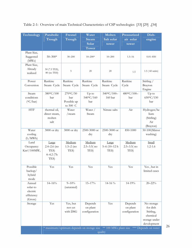
Table 2-1: Overview of main Technical Characteristics of CSP technologies [33] [29] ,[34]

Technology Parabolic Trough

Fresnel Trough

Water Steam Solar

Tower

Molten Salt solar

tower

Pressurized air solar

tower

Dish-engine

Plant Size, Suggested

(MWe) 50–300* 30–200 10–200* 10–200 1.5–16 0.01–850

Plant Size, Already realized

50 (7.5 TES), 80 (no TES) 5 20 20

1.5 1.5 ( 60 units)

Power Conversion

Rankine Steam Cycle

Rankine Steam Cycle

Rankine Steam Cycle

Rankine Steam Cycle

Rankine Cycle

Stirling / Brayton Engine

Steam conditions (*C/bar)

380*C/100 bar

270*C/50 bar

Possible up to 500 C

Up to 540*C/160

bar

540*C/100–160 bar

480*C/100–bar

Up to 650*C/150

bar

HTF thermal oil, direct steam,

molten salt

Water /steam

Water / Steam

Nitrate salts

Air Hydrogen/helium

(Stirling) Air

(Brayton) Water

cooling (L/MWh)

3000 or dry

3000 or dry

2500-3000 or dry

2500-3000 or dry

850-1000 50-100(Mirror washing)

Land Occupancy

Km2/100MWe

Large 2.4–2.6 (no

TES) 4–4.2 (7h

TES)

Medium 1.5–2 (no

TES)

Medium 2.5–3.5( no

TES)

Large 5–6 (10–12 h

TES)

Medium 2.5–3.5( no

TES)

Small 1.2-1.6

Possible backup/ hybrid mode

Yes

Yes

Yes

Yes

Yes Yes , but in limited cases

Annual solar-to electric

efficiency (Gross)

14–16%

9–10% (saturated)

15–17%

14-16 %

14-19% 20–22%

Storage Yes

Yes, but not yet

with DSG

Depends on plant

configuration

Yes

Depends on plant

configuration

No storage for dish Stirling, chemical

storage under development

* maximum/optimum depends on storage size ** 100 MWe plant size *** Depends on water quality

27

Table 2-2: Overview of main commercial characteristics of CSP technologies [33][29]

Technology Outlook for improvements

Maturity investment costs

USD/KW(2)

O & M costs

Technology Risk

Trough Limited - Proven Technology on

large scale; -Commercially viable

today

4,000–5,000 (no storage)

6,000–7,000 (7–8h storage)

Large Low

LFR Significant -Demonstration projects, first

commercial projects under construction

3,500–4,500 (no storage)

Medium Medium

Water Steam Solar Tower

Very significant -Saturated steam projects in operation -Superheated steam

demonstration projects, first

commercial projects under construction

-Commercially viable 2013 onwards

4,000–5,000 (no storage)

Medium Medium

Molten Salt solar tower

Very significant Demonstration projects, first

commercial projects Operating from late

2011.

8,000–10,000 (10th storage)

Medium Medium

Dish-engine Through mass production

-Demonstration projects, Largest

operating project is 1.5 MW;

4,500–8,000 (depending on volume production)

small High

Troughs and Central receiver power plants are the two most commercially mature and proven technologies, both having advantages and disadvantages which makes it not easy to pick one over the other.

Parabolic Trough systems using oil as HTF have solar operating temperatures restricted to 390 °C

which leads to steam temperature around 370 °C, while Tower systems can achieve higher receiver

temperatures of up to 1200 °C and steam temperatures of up to 565 °C, this gives Solar tower systems an advantage over parabolic troughs in running standards Rankine steam turbines and achieving higher annual solar to electric efficiencies (Table 2-2). Both technologies offer simple hybrid solutions with fuel oil and natural gas and can be integrated in combined cycle schemes, although the higher temperatures

28

achieved by Solar towers gains an advantage to be used in higher efficiency cycles such as the Brayton gas combined cycle. In the integrated solar combined cycle (ISCC), Solar steam from parabolic trough’s feeds the bottoming cycle with an maximum annual solar share of about 10% [35] while by using Tower systems an annual solar fraction between 10 and 25 % can be reached in molten salt towers [36] and up to 30 % in pressurized air towers [25]. As for thermal energy storage, the latest parabolic trough project with storage is the Andaso-1 plant in Spain; the 50 MWe plant incorporated 7.5 hours two tank molten storage while the SolarTres power tower in Spain with a capacity of 15 MWe incorporated 15 hour storage capacity [37].Solar towers have the potential of reaching higher amounts of storage due to the higher temperatures reached and the use of direct molten salt storage. Both technologies have modular solar components suitable for mass production, although new advancement in tower technology especially by the company eSolar offers a more modular solution , a 5 MW demonstration project has been operated successfully since 2010 [38]. In the case of land use which is one of the critical factors in the location decided in this work, Table 2-1 shows that for Molten salt solar towers with storage the land use is higher than parabolic trough plans, the land use for water/ steam type tower is close to that of parabolic troughs, with new developments promising lower land use. The Solar power company BrightSource claimed that there new tower project complex Ivanpah currently under construction will require 33 % less land than trough power plants due to increased tower heights[32]. Investment and O&M costs are shown in Table 2-2, while more complex analysis is needed to compare the total investment for parabolic trough and central receiver options, a general conclusion with the above analysis can be reached. Molten salt tower systems are the most capital intensive followed by parabolic trough’s with storage and finally by water/steam towers. Three studies were used to predict the cost reduction potential for Troughs and Solar tower systems:

U.S. Department of Energy CSP Program: Power Tower Technology Roadmap and Cost Reduction Plan [39]

International Energy Agency: Technology Roadmap Concentrating Solar Power [29]

Sargent & Lundy: Assessment of Parabolic Trough and Power Tower Solar Technology Cost and Performance Forecasts [36]

The three main drivers for cost reduction in CSP power plants are: technology improvements, economy of scale and volume production. It is worth to mention that the studies by Sandia and Sargent & Lundy compared molten salt tower system versus parabolic troughs using oil as HTF, on the other hand the EIA study considered power tower system in general against parabolic troughs using oil as HTF. The

29

analysis shown in (Table 2-3) clearly shows that the cost reduction potential for solar power towers exceeds that of parabolic trough systems. Table 2-3: Estimated current (2010) and future costs (2020) for parabolic Trough & Power Tower Systems.

Parabolic Trough Systems Power Tower Systems

Sargent & Lundy 35 % 40 %

Sandia 45 % 50 %

EIA 30 - 40 % 40 - 75 %

Four concentrating solar technologies were considered (Parabolic troughs, Solar Tower systems, Linear Fresnel and dish-engine). Using existing and projected data for large scale solar plants the simple analysis showed favourable results for solar tower option more than the other three options, it should be noted that for other case studies other options could be more favourable depending on the limiting factors, for this report the required simplicity of the total system, investment costs and modularity is three of the most important factors.

2.5 INTEGRATION OPTIONS: In this work two Integration options of Central receiver systems with conventional combined power cycles will be considered:

2.5.1 WATER / STEAM TOWER IN A NATURAL GAS FIRED COMBINED CYCLE ( HIGH

TEMPERATURE) Superheated steam is produced and mixed with superheated steam produced in the heat recovery steam generator (HRSG) hp drum, superheating is done in the HRSG. The steam turbine need to be oversized in order to accommodate for the increased amount of solar steam. In the case of a small solar share a small increase in the steam turbine size above the Combined cycle capacity results in high solar to electric efficiency and the penalty of operating the Rankine cycle at part load conditions when the solar steam is not available is small. For large solar contributions the penalty in part load Rankine cycle efficiency increases and can reach up to 10/15 %[40].Steam turbine and HRSG need to be optimized for the final solar share from the beginning which is expensive and can result in reduced efficiencies. To date this scheme has only been implemented with parabolic trough technology; however central receiver systems producing saturated steam can play the same role as parabolic troughs in the combined cycle.

2.5.2 AT

As discussimplicityworking aconjuncti

3 P

3.1 IN

This chapderived fr

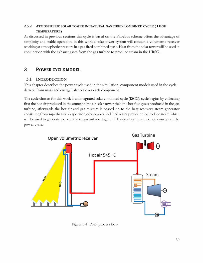
The cyclefirst the hturbine, aconsistingwill be uspower cy

ATMOSPHERI

EMPERATUR

ssed in previoy and stable at atmospherion with the

POWERCY

NTRODUCT

pter describerom mass an

e chosen for thot air producafterwards thg from supersed to generacle.

IC SOLAR TO

RE) ous sections operation, in

ric pressure inexhaust gase

YCLEMODE

TION s the power

nd energy bal

this work is aced in the atmhe hot air anrheater, evapote work in th

Fig

OWER IN NAT

this cycle is n this work an a gas fired ces from the g

EL

cycle used inances over e

an integrated mospheric airnd gas mixtuorator, econohe steam turb

gure 3-1: Plan

TURAL GAS F

based on thea solar towercombined cycas turbine to

n the simulatiach compon

solar combinr solar tower

ure is passed omizer and febine. Figure (3

nt process flo

FIRED COMB

e Phoebus scr system will cle. Heat fromo produce ste

ion, componnent.

ned cycle (ISthen the hot

d on to the heed water pre3.1) describe

ow

BINED CYCLE

cheme offerscontain a vo

m the solar toeam in the HR

nent models u

SCC); cycle bet flue gases prheat recoveryeheater to proes the simplifi

E ( HIGH

s the advantaolumetric rec

ower will be uRSG.

used in the cy

egins by colleroduced in thy steam geneoduce steam wfied concept o

30

age of ceiver sed in

ycle

ecting he gas erator which of the

31

3.2 THE SIMULATION SOFTWARE TRNSYS TRNSYS (Transient system simulation) is modular software tool used for simulation of solar systems, buildings, electrical systems and numerous other applications. TRNSYS graphical interface allows the user to choose pre-configured component represented as icons from the software library, a wide range of component models are available such as heat exchangers, electrical components, and solar thermal collectors. TRNSYS components are black boxes where the user defines a set of inputs and parameters; inputs are time dependent variable where parameters do not change with time. The system produces a set of outputs by solving sets of equations. An example of component flow diagram for a gas turbine is shown in figure (3.2).

The different types can be connected to each other where the output of one component becomes the input to the next component producing a system such as a power cycle. A special collection of TRNSYS components assembled to simulate solar thermal power generation will be used in this work; The STEC library is used extensively in this work ; it contains four component sub libraries: Rankine cycle components, Brayton cycle components, solar thermal components and thermal storage components.

The Library developed in a joint effort between three institutions DLR (German Aerospace Center), Sandia labs and IVTAN Institute for High Temperatures of the Russian Academy of Science, Russia. [41]. In this work the model will be run in 1 h time step for the whole year. The solar DNI data was obtained for a whole year from the Meteonorm software database

Gas Turbine

T combustion air

T cooling air

Inlet pressure

Mass flow

Isentropic efficiency

T OUT

Mass flow out

Actual power

Relative power

Outlet enthalpy

Figure 3-2: information flow diagram for Gas turbine

Gas Turbine

As can betower at tare used cycle is mwater madependinflows to tsecond to

Figure

e seen from fithe same temfor superhea

maintained by ass flow “to ang on the avathe three turo supply the D

e 3-3: The In

figure (3.3), homperature areating and prothe feedwateachieve com

ailable heat inrbine stages wDeaerator.

ntegrated Sola

ot exhaust gae combined inoducing saturer pump whicplete evapor

nput coming where it is ex

ar Combined

ases from then the flow mrated steam, tch is connecteration; the evfrom the ho

xtracted twic

d Cycle in TR

e gas turbine amixer before b

the feedwateed to the evapvaporator wilot air and the ce, first to su

RNSYS

at 544 ͦ C andbeing passed er flow throuporator that “ll demand a flue gases. S

upply the feed

d hot air fromto the HRSG

ugh the botto“demands a ccertain mass

Superheated sdwater heate

32

m solar G and oming ertain s flow steam er and

33

3.3 COMPONENT MODELS The power plant is composed of three main sub-cycles; the gas turbine cycle, steam turbine and solar air cycle. Each one of these cycles contains subsystems such as compressor, heat exchangers, heliostat field and many others. These subsystems are realised by constructing component models in a MATLAB function and a TRNSYS project. In the following sections detailed descriptions of the thermodynamic components will be introduced.

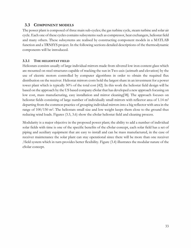
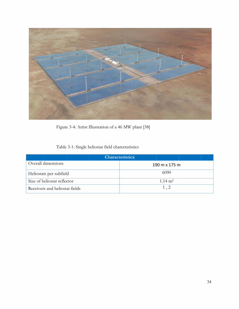
3.3.1 THE HELIOSTAT FIELD Heliostats consists usually of large individual mirrors made from silvered low iron content glass which are mounted on steel structures capable of tracking the sun in Two-axis (azimuth and elevation) by the use of electric motors controlled by computer algorithms in order to obtain the required flux distribution on the receiver. Heliostat mirrors costs hold the largest share in an investment for a power tower plant which is typically 50% of the total cost [42]. In this work the heliostat field design will be based on the approach by the US based company eSolar that has developed a new approach focusing on low cost, mass manufacturing, easy installation and mirror cleaning[38]. The approach focuses on heliostat fields consisting of large number of individually small mirrors with reflector area of 1.14 m2 departing from the common practice of grouping individual mirrors into a big reflector with area in the range of 100/150 m2. The heliostats small size and low weight keeps them close to the ground thus reducing wind loads. Figures (3.5, 3.6) show the eSolar heliostat field and cleaning process.

Modularity is a major objective in the proposed power plant; the ability to add a number of individual solar fields with time is one of the specific benefits of the eSolar concept, each solar field has a set of piping and auxiliary equipment that are easy to install and can be mass manufactured, in the case of receiver maintenance the solar plant can stay operational since there will be more than one receiver /field system which in turn provides better flexibility. Figure (3.4) illustrates the modular nature of the eSolar concept.

Overall d

Heliostat

Size of he

Receivers

Figure

Table

dimensions

s per subfield

eliostat reflec

s and heliosta

e 3-4: Artist I

3-1: Single h

d

ctor

at fields

Illustration o

heliostat field

Cha

of a 46 MW p

d charecteristi

aracteristics

plant [38]

tics

s

1990 m x 175 m

6090

1.14 m2 1 , 2

m 

34

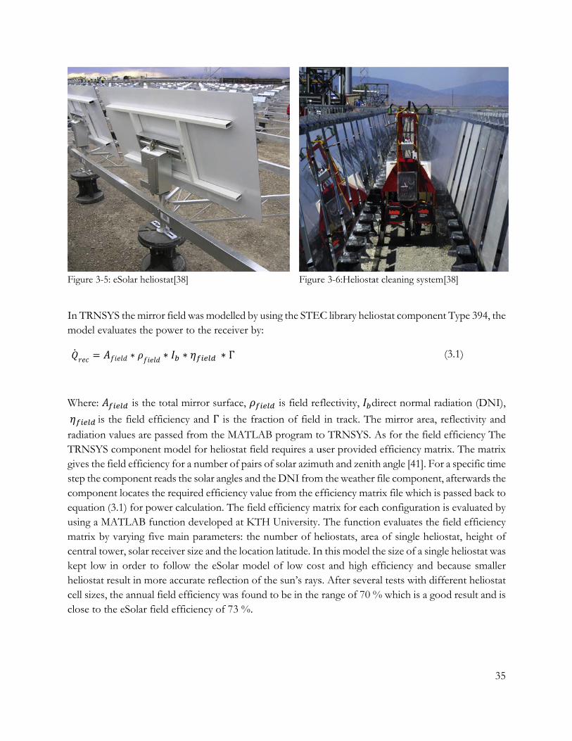
Figure 3-5

In TRNSYmodel ev=

Where: is radiation TRNSYSgives the step the ccomponeequation using a Mmatrix bycentral tokept low heliostat rcell sizes,close to t

5: eSolar helios

YS the mirrovaluates the p∗

is the t

the field effivalues are p

S componentfield efficienomponent re

ent locates th(3.1) for pow

MATLAB funy varying fiveower, solar rec

in order to result in mor the annual fhe eSolar fie

stat[38]

or field was mpower to the ∗ ∗total mirror s

ficiency and Γassed from tt model for hcy for a numbeads the solare required ef

wer calculationction develoe main paramceiver size anfollow the e

re accurate refield efficiencld efficiency

modelled by usreceiver by:

∗ Γ

surface, Γ is the fractthe MATLABheliostat fieldber of pairs o

r angles and thfficiency valuon. The field oped at KTHmeters: the nnd the locatioeSolar modeleflection of thcy was found of 73 %.

Figure

sing the STEC

is field ref

tion of field B program tod requires a uof solar azimuhe DNI from

ue from the efefficiency m

H University. number of heon latitude. Inl of low coshe sun’s raysto be in the

e 3-6:Heliosta

C library helio

flectivity, d

in track. Tho TRNSYS. Auser provideduth and zenit

m the weather fficiency mat

matrix for eachThe functio

eliostats, arean this model tt and high e

s. After severrange of 70 %

at cleaning sys

ostat compon

direct norma

he mirror areAs for the fi

d efficiency mth angle [41]. r file compontrix file whichh configuratin evaluates ta of single hthe size of a sefficiency andral tests with % which is a

tem[38]

nent Type 39

(3.1)

l radiation (D

ea, reflectivityeld efficiency

matrix. The mFor a specificent, afterwardh is passed baion is evaluatthe field efficheliostat, heigingle heliostad because smdifferent helgood result a

35

94, the

DNI),

ty and y The

matrix c time ds the ack to ted by ciency ght of at was maller liostat and is

Losses ocmajor facthe reflecbetween teffect of treflected from diff[43].

Figure 3-

Shadowinblocking lit from reand sun a

3.3.2 TAir is mositting onbottominfrom the library. Tsupport th

ccurs that inftor affecting

cted power pthe sun’s beatwo heliostatrays is almo

ferent positio

7: The cosin

ng losses occulosses occur

eaching the reangles and ca

THE TOWER ved through

n top of a tong cycle. In th

Hydronics liThe tower hei

he weight of

fluence the fifield efficien

per unit area am and a line mirrors on dst pointing tons of the mir

e effect for t

ur at low sunone heliostat

eceiver. Shadan be determi

pipes by the ower. Afterwhis work the ibrary) due toight is approxreceiver and

ield efficienccy ,the heliosis decreasedfrom the hel

different direco the receiverror and the r

two heliostats

n angels whent blocks the reowing and blined by the u

use of a centwards the hot

tower was mo the fact thaximately 100give access to

cy these inclutats are not g

d by the cosinliostat to thections. Helioer whereas foreceiver. For

s in opposite

n one heliostaeflected radialocking lossesuse of compu

trifugal air blt air is move

modelled as sat no compon0 meters; struo maintenanc

ude: Cosine egenerally perpne of half the receiver[43]ostat A has higor heliostat Bdetailed calcu

e directions f

at shadows onation from a hs depends onuter analysis

lower on the ed to the HRseries of hot nent for the

uctural mass oce work for th

effect losses apendicular to he angle θ de .Figure (3.7)gher cosine eB higher lossulation of co

from the tow

ne or more hheliostat behi

n tower heightechniques.

way to the vRSG to prodand cold ductower is avaiof the tower he pipe netwo

are considerethe solar radi

efined as the ) shows the cefficiency sincses occur resusine losses re

wer [43]

heliostats behiind it and pret, heliostat sp

olumetric recduce steam ict pipes (Typilable in the Sshould be ab

ork situated in

36

ed the iation, angle

cosine ce the ulting

efer to

ind it, events pacing

ceiver in the pes 31 STEC ble to nside.

Ambient to the recHeat tranthe hot anvalue to t=Convectivnumber acalculate

Figure 3-

air is moved ceiver outlet nsfer, insulationd cold ductthe TRNSYS

∆

ve heat transaccording to Reynolds an

8: Solar towe

by the centritemperatureon material thts. Over all hS model:

sfer coefficienthe correlatiod Prandtls nu

ers in Califor

fugal blower ; afterwards hickness, pre

heat loss coef

nts inside anon by Gnielinumbers.

rnia (Sierra co

from groundthe hot air is

essure losses afficient is calc

d outside thenski , a fluid

ommercial de

d level up to ts moved dowand investmeculated for th

e duct is evalvelocity of 1

emonstration

the receiver wwn the hot dent costs mushe hot duct b

luated by the10 m/s was a

n plant) [38]

where it gets huct to the H

st be accountebefore passin

(3.2)

e use of Nussassumed to

37

heated HRSG.

ed for ng the

selt

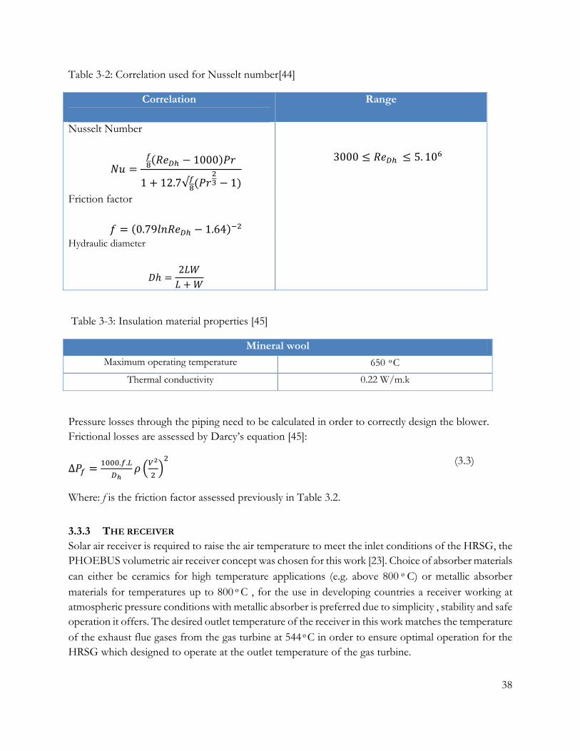
38

Table 3-2: Correlation used for Nusselt number[44]

Correlation

Range

Nusselt Number = ( − 1000)1 + 12.7√ ( − 1)

3000 ≤ ≤ 5. 10

Friction factor = (0.79 − 1.64)

Hydraulic diameter ℎ = 2+

Table 3-3: Insulation material properties [45]

Mineral wool

Maximum operating temperature 650 ͦ C

Thermal conductivity 0.22 W/m.k

Pressure losses through the piping need to be calculated in order to correctly design the blower. Frictional losses are assessed by Darcy’s equation [45]:

∆ = . .

(3.3)

Where: f is the friction factor assessed previously in Table 3.2.

3.3.3 THE RECEIVER Solar air receiver is required to raise the air temperature to meet the inlet conditions of the HRSG, the PHOEBUS volumetric air receiver concept was chosen for this work [23]. Choice of absorber materials can either be ceramics for high temperature applications (e.g. above 800 ͦ C) or metallic absorber materials for temperatures up to 800 ͦ C , for the use in developing countries a receiver working at atmospheric pressure conditions with metallic absorber is preferred due to simplicity , stability and safe operation it offers. The desired outlet temperature of the receiver in this work matches the temperature of the exhaust flue gases from the gas turbine at 544 ͦ C in order to ensure optimal operation for the HRSG which designed to operate at the outlet temperature of the gas turbine.

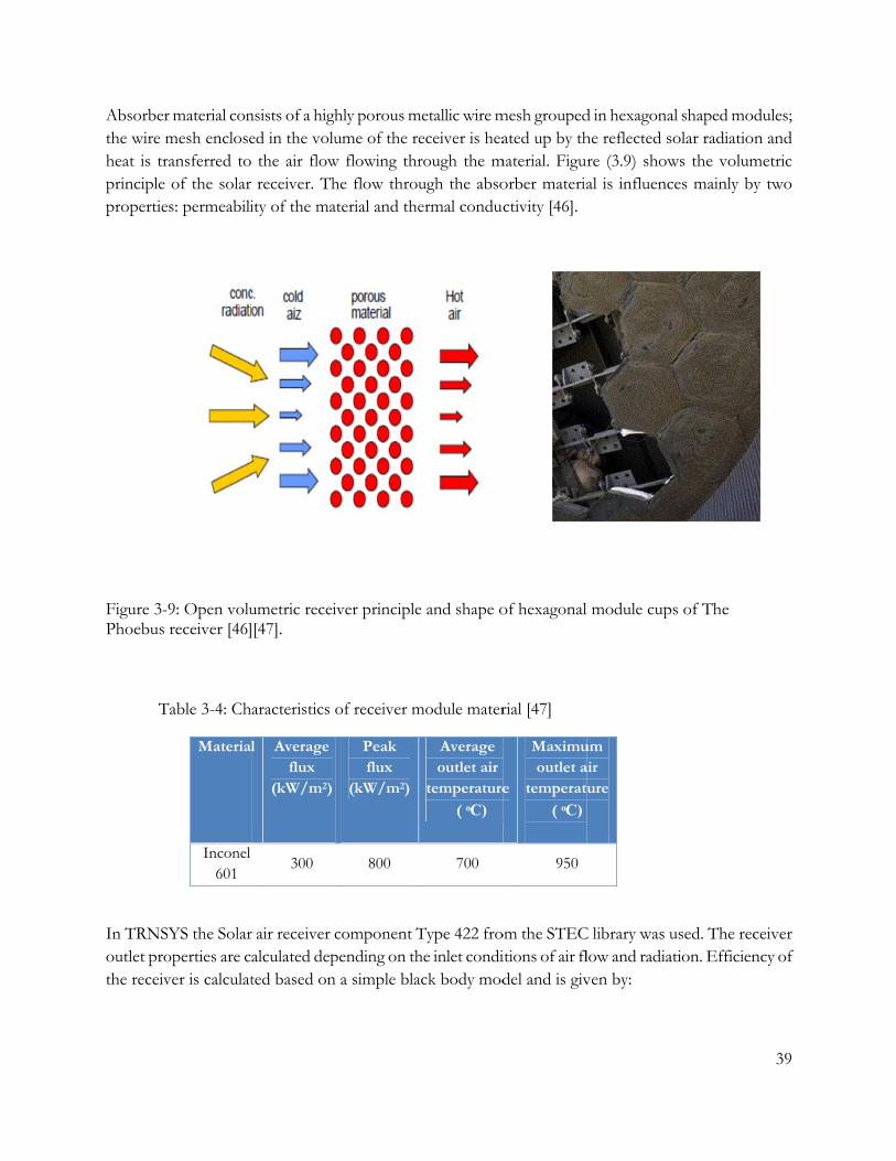
Absorberthe wire mheat is trprinciple propertie

Figure 3-Phoebus

T

In TRNSoutlet prothe receiv

r material conmesh encloseransferred to

of the solar s: permeabili

9: Open volureceiver [46]

Table 3-4: Ch

Material

Inconel 601

SYS the Solaroperties are cver is calculat

nsists of a highed in the volu the air flowreceiver. Th

ity of the ma

umetric recei[47].

aracteristics

l Average flux

(kW/m2)

300

r air receiver calculated depted based on

hly porous mume of the re

w flowing thrhe flow throuaterial and the

iver principle

of receiver m

Peak flux

(kW/m2)

800

component Tpending on thn a simple bla

metallic wire meceiver is hearough the mugh the absoermal conduc

e and shape o

module mater

Averageoutlet air

temperature

( ͦC)

700

Type 422 frohe inlet condiack body mod

mesh groupedated up by th

material. Figurorber materiactivity [46].

of hexagonal

rial [47]

e

Maximuoutlet a

temperat

( ͦC)

950

om the STECitions of air fldel and is giv

d in hexagonahe reflected sre (3.9) showal is influenc

l module cup

um air ure

C library was ulow and radiaven by:

al shaped modsolar radiationws the volumces mainly by

ps of The

used. The recation. Efficien

39

dules; n and

metric y two

ceiver ncy of

40

= − . (3.4)

Where ε: the emissivity of the absorber material is set to 0.85 and the optical efficiency is set to 0.90.

4 = 0.5. , + , + 273.15 (3.5)

The pressure drop through the wire mesh material of the receiver is approximated by using one correlation developed by Mccorquodala et al for flow of air through porous material of rock beds[48]: Δ = 4.74 ( )⁄ + 166 . (3.6)

Where: L is the width of the receiver module; GO is the mass velocity of air in material (air mass flow rate divided by the module area). μ is the viscosity of air , α is the shape factor of the material grains and is set to 1.4 and ε is the absorber open porosity.

3.3.3.1 RECEIVER CONTROL STRATEGY

The outlet air temperature at of the receiver desired value is (544 °C) equalling the temperature of the exhaust gases from the gas turbine, in order to ensure that the desired temperature do not increase above this value a temperature limit control is attached to the receiver, a second control loop is connected to heliostat field component to ensure that the maximum flux limit is not violated; the control will force the heliostat field to “defocus” if the flux limit is violated. Air flow through the receiver is set by a control switch , after repeated trials it was found that starting the air pump from 10:00 AM to 16:00 PM will ensure that the receiver maintain the desired outlet temperature.

3.3.4 THE GAS TURBINE The gas turbine using natural gas as fuel provides the main power source to the ISCC; exhaust gases from the turbine combined with hot air coming from the solar tower receiver provide necessary heat to produce steam in the heat recovery steam generator.

At night time the system is operated as a regular combined cycle with all the heat produced by the exhaust gases, SGT-800 gas turbine from Siemens was chosen for this work, this turbine has been widely used in combined cycle applications table (3.5) lists technical details of the gas turbine.

The compspecifies chosen fospecifies tnatural gaset to 120

The turbiuser specmanufactstandard

pressor modan isentropicor the air inlethe lower heaas was taken f00 ͦ C [49].

ine model simcified isentropturer’s specifiTRNSYS ge

Table 3-5:

Power G Compre Exhaust

Combus Exhaust

el in TRNSYc efficiency inet. The combating value anfrom the turb

milar to the cpic efficiency

fication sheetnerator comp

Figure 3

Technical sp

Generation:

ssor pressure

Gas flow :

stion tempera

temperature

YS calculates n this work abustion chamnd the mass rbine specifica

compressor my, an isentrop. Net electricponent with

3-10: The SG

pecifications

(I

e ratio: 1

13

ature ~

e: 5

the outlet coa value of 0.8mber model dratios of the eation sheet. Co

model calculapic efficiencycal power is c

a user specif

GT-800 [49]

for SGT-800

ISO) 47.0 M

19.9:1

31.5 kg/s

~ 1200° C

544° C

onditions from9 was chosen

describes an aelements in thombustion ch

ates outlet coy of 0.90 showalculated by cfied mechani

0 gas turbine

MW(e)

m the inlet con. A pressureadiabatic comhe fuel, lowehamber outle

onditions fromwed the closconnecting thical efficiency

e [49]

onditions; thee drop of 0.0mbustion; ther heating valuet temperatur

m inlets by usest result withe gas turbiny of 0.99.

41

e user 3 was e user ue for re was

sing a th the

ne to a

42

3.3.5 FLOW MIXER Hot air from the solar receiver mixes with hot flue gases from the gas turbine before entering the HRSG. The simple flow mixer model in TRNSYS is simulated by using an equation block where a mass and energy balances is performed before passing the hot mixture to the superheater component in the HRSG.

3.3.6 THE HEAT RECOVERY STEAM GENERATOR Hot air from the solar receiver and Exhaust flue gases from the turbine are transferred to the HRSG which consists of Superheater, Evaporator and Economizer.

In the economizer the feed water temperature is raised to close saturation point. In the evaporator the feed water evaporates at constant pressure and temperature producing saturated steam. The steam is then passed to the Superheater to raise its temperature to the desired turbine inlet conditions. Figure (3-12) shows the Temperature / Energy diagram for the Single pressure HRSG.

Figure 3-12: Energy/temperature diagram of a single-pressure HRSG

0 5 10 15 20 25 30 35 40 45200

250

300

350

400

450

500

550

600

Energy Transfer [MW]

Tem

pera

ture

[°C

]

Energy/Temperature diagram for a single-pressure HRSG

Superheater

Economizer

Approach Temperature

Evaporator

Pinch Point

Hot Air

Flue Gas Hot Mixture

Figure 3-11: Flow Mixer

43

In order to calculate relevant values for the TRNSYS component models such as the heat exchanger UA values and effectiveness, a separate model was built in MATLAB software environment. Two approaches have been used in the model, a pinch point analysis in order to obtain the steam mass flow and effectiveness-NTU method for determining the UA (overall heat transfer conductance-area) values and the effectiveness of the heat exchangers.

Pinch point analysis directly affects the amount of steam to be generated in the HRSG; the evaporator pinch point temperature can be defined as the difference between evaporator temperature on the cold side (water/steam) and the outlet temperature on the hot side( gas exhaust/hot air). The economizer approach temperature can be defined as the difference between the saturation temperature in the drum and the outlet economizer temperature, this difference helps to prevent evaporation in the economizer.

The lower the pinch point temperature difference the more heat can be collected by the heat exchangers; however the required heating surface area also increases resulting in increased costs. Typical values for pinch point range from 8 to 15 K. typical values for economizer approach temperatures range from 5 to 12K[12] . Table (3.6) show the values used for pinch point and approach temperatures in the HRSG.

Table 3-6: HRSG design parameters

Pinch Point 10 ͦ C Economiser water approach 5 ͦ C

Steam Turbine inlet conditions 100 Bar , 480 ͦ C

Pressure drop superheater 1 Bar Pressure drop economiser 0.7 Bar

The Matlab function XSteam [50] for evaluating steam and water properties was used to evaluate enthalpies and temperatures of the required streams.

The heat available to evaporator and superheater from turbine exhaust/hot air is calculated from: = , − + ℎ (3.7)

And so the mass of steam can be calculated from: = ℎ − (3.8)

44

The effectiveness-NTU design method [44] is used for calculating UA values and effectiveness for the heat exchanger before passing it to TRNSYS. The effectiveness is defined as the ratio of the actual heat transfer achieved to the maximum possible heat transfer achieved.

= ⁄

(3.9)

In order for to be evaluated the heat capacitance of the hot and cold streams need to be calculated: = ∗ (3.10)

= ∗ (3.11)

The average specific heat for the steam/water stream is acquired from the XSteam function in Matlab, for the flue gases and dry air the function CpGAS was developed in Matlab based on the work of Walsh [51]. The maximum heat transfer can then be calculated from: = , − , (3.12)

Where = ( , ) (3.13)

The effectiveness of a heat exchanger is a function of two parameters: the number of transfer units (NTU) and the capacitance rate ratio of the two streams (Cr) which is defined as: = ⁄ (3.14)

Where = ( , ) (3.15)

The NTU is defined as:

= ⁄ (3.16)

Table (3.7) lists the different effectiveness-NTU relations for different heat exchangers, economizer and Superheater are treated as a Counterflow heat exchanger where the evaporator and condenser are treated as a special case due to the infinite heat capacity of the steam/feed water.

45

Table 3-7: Effectiveness-NTU relations for different heat exchanger types [44]

Exchanger Type Relation Condition

Counter Flow

= 1 − 1− 1 < 1

= 1 − = 1

Evaporator/Condenser

= − (1 − ) = 0

The UA values for the heat exchangers at nominal conditions can be found from the above relations and passed on to the TRNSYS models.

3.3.7 THE STEAM TURBINE The steam turbine model consists of a high pressure stage, intermediate pressure stage and a low pressure stage. Steam extraction to the feedwater heaters is taken from the first and second stage. Outlet power of the steam turbine is the sum of all three stages.

The user specifies values for inlet pressure, outlet pressure, reference mass flow rate and isentropic efficiency. The model evaluates the inlet pressure from the outlet pressure using Stoidolas law of the eclipse.[41]. Isentropic efficiencies of the Turbine stages are calculated based on the work of [52] in MATLAB before passing the values to TRNSYS using: = 0.835 + 0.02 (3.17)

Where: is the volumetric flow rate in m3/s.

For the first turbine stage can be calculated from the ratio of mass flow of steam to the density, since the first stage temperature is know and equals TSH , the density can be calculated with the XSteam

function. For the second and third stages the outlet temperatures are unknown therefore is calculated using a polytrop expansion using: = ( ) ⁄ (3.18)

The polytrop expansion coefficient (n) is set to 1.32[52].

Steam inlet

Extracted steam

Steam to the next stage

Figure 3-13: Steam turbine stage

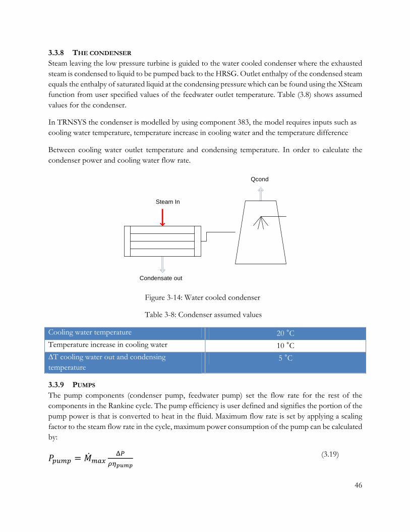
46

3.3.8 THE CONDENSER Steam leaving the low pressure turbine is guided to the water cooled condenser where the exhausted steam is condensed to liquid to be pumped back to the HRSG. Outlet enthalpy of the condensed steam equals the enthalpy of saturated liquid at the condensing pressure which can be found using the XSteam function from user specified values of the feedwater outlet temperature. Table (3.8) shows assumed values for the condenser.

In TRNSYS the condenser is modelled by using component 383, the model requires inputs such as cooling water temperature, temperature increase in cooling water and the temperature difference

Between cooling water outlet temperature and condensing temperature. In order to calculate the condenser power and cooling water flow rate.

Steam In

Condensate out

Qcond

Figure 3-14: Water cooled condenser

Table 3-8: Condenser assumed values

Cooling water temperature 20 °C Temperature increase in cooling water 10 °C ∆T cooling water out and condensing temperature

5 °C

3.3.9 PUMPS The pump components (condenser pump, feedwater pump) set the flow rate for the rest of the components in the Rankine cycle. The pump efficiency is user defined and signifies the portion of the pump power is that is converted to heat in the fluid. Maximum flow rate is set by applying a scaling factor to the steam flow rate in the cycle, maximum power consumption of the pump can be calculated by: = (3.19)

47

Where: M ̇ max is the maximum flow rate through the pump components, Δ is the pressure difference before and after the pump, is the fluid density and is the pump efficiency, a value of 0.85 was set for the two pumps.

3.3.10 OPEN FEEDWATER HEATER (DEAERATOR) The open feedwater heater is modelled as mixing water preheater with three inlets and one outlet. Open feedwater heater is used to remove dissolved gases and non-condensables from the feedwater. Extracted steam from second turbine stage and hot condensate flow coming from the closed feedwater heater are used to preheat the feedwater coming from the condenser.

Mass flow rate of the outlet feedwater equals the sum of all three inlet mass flows, the demanded mass flow of the extraction steam can be found by conducting an energy balance around the Deaerator. ℎ + _ ℎ _ + , ℎ , = , ℎ , (3.20)

Where: _ can be found by applying an energy balance over the closed feedwater heater as shown later. Enthalpies of the inlet /outlet streams are found by using the XSteam function with the related temperatures /pressures.

3.3.11 CLOSED FEEDWATER HEATER In the closed feedwater heater, high pressure water comes into contact with condensing steam extracted from the first turbine stage. Heat transfer occurs in three zones; desuperheating zone where superheated steam becomes saturated steam, condensing zone where saturated steam condenses to saturated liquid and the subcooling zone where the saturated liquid is cold to a temperature below the saturation temperature. In the TRNSYS model the closed feedwater heater is represented by a steam condenser and a subcooler, desuperheating is neglected. UA values for both components are computed using the NTU-effectiveness method in MATLAB before passing them to TRNSYS.

Extracted steam Feedwater, inlet

Condensed steam Feedwater, outlet

Figure 3-15: open feedwater heater flow diagram

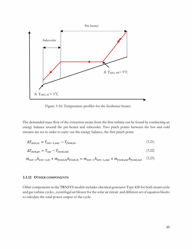
48

Figure 3-16: Temperature profiles for the feedwater heater.

The demanded mass flow of the extraction steam from the first turbine can be found by conducting an energy balance around the pre-heater and subcooler. Two pinch points between the hot and cold streams are set in order to carry out the energy balance, the first pinch point: ∆ , = , − , (3.21) ∆ , = − , (3.22) ℎ , + , ℎ , = ℎ , + , ℎ , (3.23)

3.3.12 OTHER COMPONENTS Other components in the TRNSYS models includes electrical generator Type 428 for both steam cycle and gas turbine cycles , centrifugal air blower for the solar air circuit and different set of equation blocks to calculate the total power output of the cycle.

Subcooler

Pre-heater

∆ TMIN, PR= 9°C

∆ TMIN, SC= 5°C

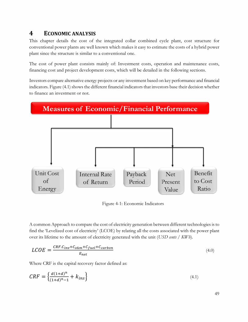
4 EThis chaconventioplant sinc

The costfinancing

Investorsindicatorsto finance

A commofind the ‘Lover its li

Where CR=

ECONOMICapter details onal power pce the structu

t of power pg cost and pro

s compare altes. Figure (4.1)e an investm

on ApproachLevelized coifetime to the= .RF is the cap( )( )

CANALYSIthe cost of

plants are welure is similar

plant consistoject develop

ernative energ) shows the d

ment or not.

h to compare st of electricie amount of

&pital recovery+

Sf the integrall known whito a convent

s mainly of:pment costs,

gy projects ordifferent finan

Figure 4

the cost of elity’ (LCOE) electricity ge

y factor defin

ated collar cch makes it etional one.

Investmentwhich will b

r any investmncial indicato

4-1: Econom

lectricity genby relating al

enerated with

ned as:

combined cyeasy to estima

t costs, operbe detailed in

ment based onrs that invest

mic Indicators

eration betwll the costs as

h the unit (US

ycle plant, cate the costs

ration and mthe followin

n key performtors base their

s

ween differentssociated witSD cents / KW

cost structurof a hybrid p

maintenance ng sections.

mance and finr decision wh

t technologieth the power Wh).

(4

(4.1)

49

re for power

costs,

nancial hether

es is to plant

4.0)

50

Where CINV is the total investment cost for the project, CO&M the operation and maintenance costs,

CFUEL is the fuel costs for running the gas turbine, CCARBON is the carbon emissions costs and ENET is the annual net electric power produced by the integrated solar combined cycle power plant. The capital recovery factor (CRF) accounts for the time value of money for the investment costs at a specific interest rate (d) and over a uniform specified period of time (n). It should be noted that only the generation costs are included in the analysis of the power system, transmission and distribution costs are out of the project scope. In this work the interest rate will be set to 10 % based on the values issued by the World Bank for the ISCC plant in morocco (Ain Beni Mathar) that was completed in 2011 as for the lifetime of the plant will be set to 30 years. Table (4.1) lists values for different components used in the LCOE such as fuel and water costs.

Table 4-1: Costs / Prices and economical settings (Sources: [53][a], [54][b], [55][c], [56][d]

Component Abbreviation Value Unit

Discount ratea D 10 %

Insurance Rate kINS 1 %

Life time N 25 Years

Natural gas costb CFuel 10 USD/MMBTU

Fresh water costc CWater 1 USD/1000 L

Carbon taxd CCarbon 0.688 USD/MWh

Figure (4.2) lists the estimated Levelized cost of electricity for new plant concepts [54], it can be seen that stand alone solar thermal technologies have the highest figure due to the high investment costs while the combined cycle concepts have one of the lowest; which leads to the conclusion that mix between the two technologies can lead to favourable LCOE levels.

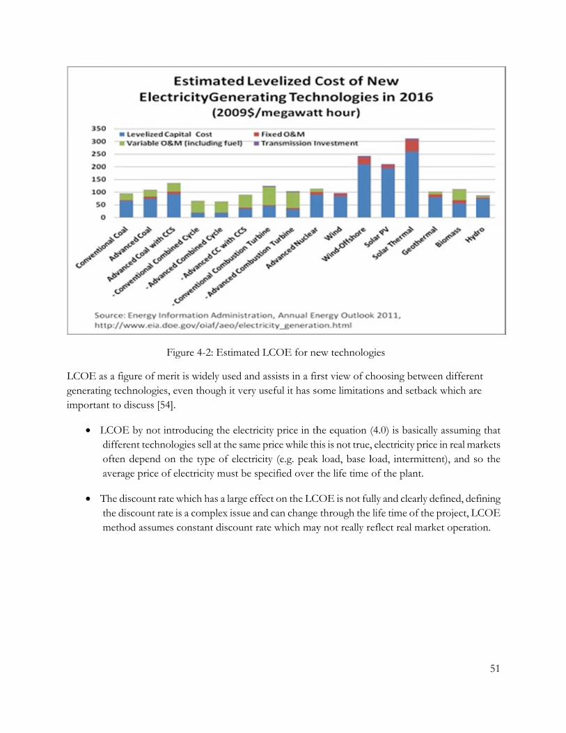
LCOE asgeneratinimportan

Ldoa

Ttm

s a figure of mng technologint to discuss [

LCOE by notdifferent techoften dependaverage price

The discount rhe discount r

method assum

Figure 4-2:

merit is wideies, even thou[54].

t introducinghnologies sell d on the type

of electricity

rate which harate is a compmes constant

: Estimated L

ly used and augh it very u

g the electriciat the same p

e of electriciy must be spe

as a large effeplex issue andt discount rat

LCOE for ne

assists in a firseful it has so

ity price in thprice while thty (e.g. peakecified over t

ect on the LCd can change te which may

ew technolog

rst view of chome limitatio

he equation (his is not true,k load, base lthe life time

COE is not fue through the y not really re

gies

hoosing betwons and setba

(4.0) is basic, electricity prload, intermiof the plant.

ully and clearlylife time of teflect real ma

ween differenack which ar

ally assumingrice in real maittent), and s

y defined, defthe project, Larket operati

51

nt re

g that arkets so the

fining LCOE ion.

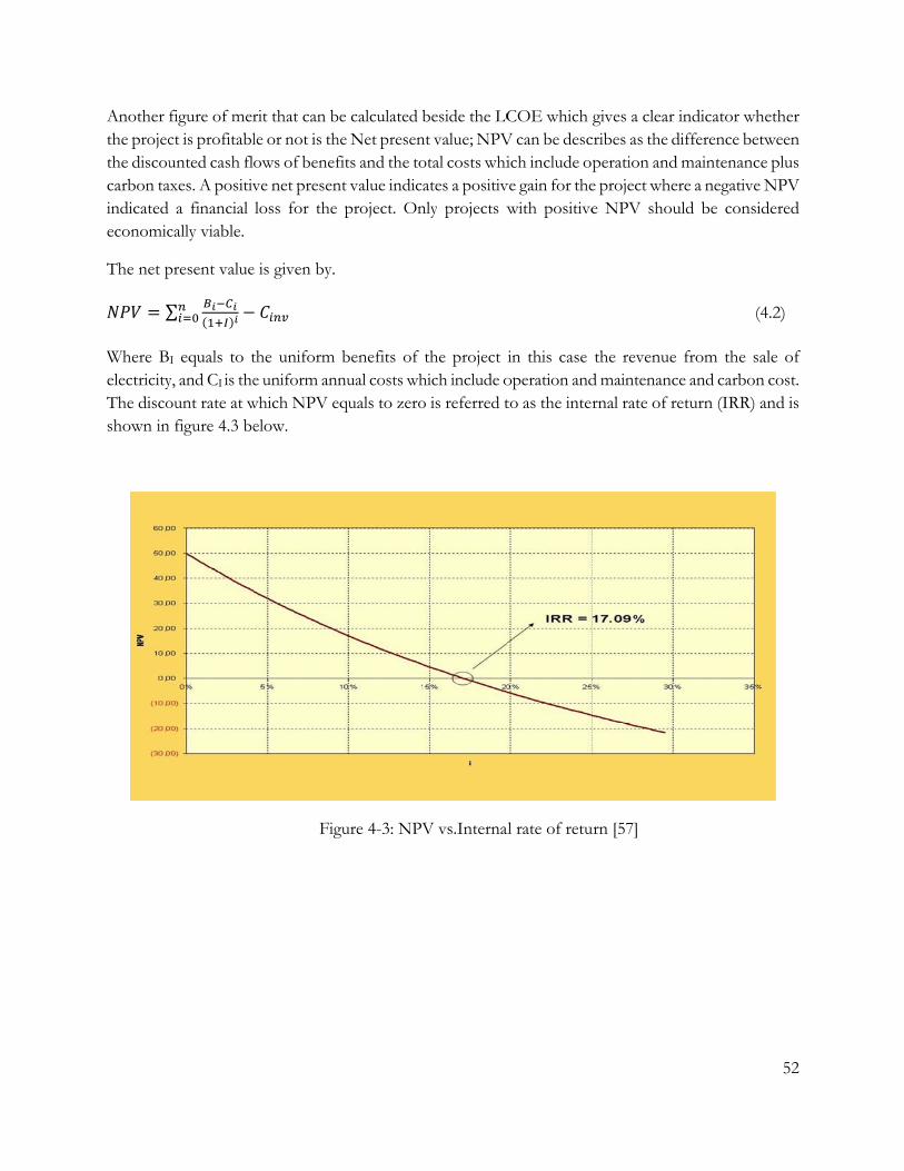
Another the projecthe discoucarbon taindicated economic

The net p= ∑Where BelectricityThe discoshown in

figure of merct is profitablunted cash fl

axes. A positiva financial

cally viable.

present value∑ ( ) −I equals to t

y, and CI is theount rate at wn figure 4.3 be

rit that can ble or not is thows of benefve net presenloss for the

e is given by. −

the uniform e uniform ann

which NPV eelow.

Fig

be calculated bhe Net presenfits and the tont value indic

project. On

benefits of nual costs wh

equals to zero

gure 4-3: NPV

beside the LCnt value; NPVotal costs whiates a positiv

nly projects w

the project ihich include oo is referred t

V vs.Internal

COE whichV can be descich include o

ve gain for thewith positive

in this case operation andto as the inter

al rate of retu

gives a clear cribes as the dperation ande project whee NPV shou

the revenued maintenancrnal rate of r

urn [57]

indicator whdifference betd maintenanceere a negative uld be consi

(4

from the sace and carbonreturn (IRR) a

52

hether tween e plus NPV dered

4.2)

ale of n cost. and is

53

4.1 COST FUNCTIONS In order to calculate the total costs of the plant (investment, operation and maintenance and fuel), cost functions for the conventional combined cycle components were adapted from the work of Pelster[52] with modifications introduced by Spelling [58].The work of Pelster is originally based on Frangopoulos[59].

To take into account the inflation effects from the year where the original cost functions, the Marshal and Swift equipment cost index for 2011[60] is multiplied by each cost function. For example he cost index for relating to the year 1991 is calculated as:

& = && = . . = 1.662 (4.3)

4.2 COST FUNCTION OF THE GAS TURBINE CYCLE Cost functions for the gas turbine components are based on original models by Frangopoulos with modifications by Pelster, the Marshal and Swift index for the year of Frangopoulos s work (1991) equals to 930.6.

4.2.1 COMPRESSOR The cost function for the compressor is given by: = 1. , ,

. Π , ln Π & (4.4)

, is the reference mass flow of air through the compressor and has a value of 515 kg/s, Π , is the reference pressure ratio has a value of 15 and c1 has a value of 27.7 (kg/s)-0.7.

Is the correction factor for the efficiency of the compressor and is given by: = (4.5)

Where the polytropic efficiency of the compressor, the constant C2 is has a value of 0.96, which accounts for the increase in efficiency since the time of original publication of Pelster’s work.

4.2.2 COMBUSTOR The cost function for the combustion chamber is given by: = 1. , ,

. & (4.6)

Where is the exhaust mass flow of the combustion chamber at design conditions, , is the reference mass flow rate with a value of 460 kg/s, and c1 has a value of 27.7

54

(kg/s)-0.7. And represent correction factors for the temperature and pressure drop, and is given by equations (4.7, 4.8) respectively. = 1 + 0.025. ( − 1600) (4.7) = . (4.8)

Where is the outlet temperature and the pressure drop in the combustion chamber.

4.2.3 TURBINE UNIT Cost function for the turbine is similar to that of the compressor and is given by: = 1. , ,

. Π , ln(Π ) (4.9)

The constant c1 have a value of 12.4 (kg/s)-0.7, exhaust reference mass flow a value of 460 kg/s and the turbine reference pressure ratio equals 15. The efficiency correction factor is calculated using equation (4.5) with the difference in the value of C2 which is 0.94; the temperature correction factor is calculated using equation (4.7).

4.2.4 TURBINE AUXILIARIES Auxiliary equipment costs in the gas turbine must be included and is given by: = , ,

. (4.10)

For a reference power output of 160MW ( , ) the reference purchase cost ( , ) equals 4 million USD.

4.3 COST FUNCTIONS FOR THE STEAM CYCLE Cost functions for the steam cycle like those of the gas turbine cycle are also taken from Pelster’s work [52].

4.3.1 HRSG The total cost of the HRSG includes the cost functions of all heat exchangers, piping, gas conduit and pumps.

55

= ( + + + ) & (4.11)

The cost function for heat exchangers includes the cost of (superheater, evaporator, economizer and feedwater heater), where the function for a single heat exchanger is given by: = ∑ . , . , . (4.12)

Where C1 equals to 3650$/(kW/K)0.8. K is given by = ∆ , (4.13)

Where ∆ , is the log mean temperature difference between the hot and cold streams of each heat

exchanger. The pressure correction factor is a function of live steam pressure and is given by: = 0.0971. +0.9029 (4.15)

The temperature correction factors are given by:

, = 1 + , (4.16)

, = 1 + , (4.17)

The cost function for piping and gas conduit are given by: = ∑ . , (4.18)

= . (4.19)

Where C2 equals 11820$/ (kg/s) and C3 = 658$/ (kg/s) 1.2.

4.3.2 STEAM TURBINE The cost of the steam turbine unit includes the turbogenerator plus the alternator as a function of the power output and is given by: = , & (4.20)

Where represents the specific costs. = , . (4.21)

56

Cref and Pref were taken from the work of Pelster and values were chosen that fits the current plant Size. The value for Cref is 275$/kW which corresponds to a Pref of 25MW. A temperature correction is Applied. = 1 + 0.096. ( − 866) (4.22)

4.3.3 TURBINE AUXILIARIES Cos function for piping and auxiliary equipment of the steam turbine unit is given by: = , .

(4.23)

In the work of Pelster a reference cost value of 10 Million USD is used for a 75MW combined cycle without reheat.

4.3.4 PUMPS Cost functions for the feedwater and condensate pumps are given b: = 422. . 1.41 & (4.24)

Where is the efficiency correction factor and is given by = 1 + ., (4.25)

The pump isentropic efficiency is set to 0.85.

4.3.5 CONDENSER AND COOLING TOWER Total cost of the condensing unit includes the cost of the steam condenser and cooling tower. = + (4.26)

The steam condenser cost is calculated as a function of the condensing area ACOND and the cooling water flow rate. = ( + ) & (4.27)

57

Where C1 is 248$/m2 and C2 = 659$(kg/s). The condensing area is found by

= .∆ (4.28)

Where the overall heat transfer coefficient k = 2200W (m2/K). ∆ Is the log mean temperature difference.

The investment for the cooling tower is given by. = 72 3 . ∆ , ∆ , . 2.35 & (4.29)

Where the factor 2.35 is introduced to take into account the cost associated with the foundations and basin. ∆ , is the temperature correction factor taking into account the increase in cost due to the small

temperature difference between the main cooling water temperature and = − 2⁄ and the wet bulb temperature of air which can be read from the weather data in TRNSYS.

∆ , = −0.6936. ln( − ) + 2.8981 (4.30)

The factor ∆ , accounts for the temperature reduction in the cooling tower and is given by.

∆ , = −0.0013. ∆ + 0.0144. ∆ + 0.0929. ∆ + 0.501 (4.31)

4.4 COST FUNCTIONS FOR THE SOLAR COMPONENTS

4.4.1 THE HELIOSTAT FIELD Cost functions for the Heliostat field are taken from the work of Kistler, total cost of the heliostat field is a function of total mirror size, wiring costs and required land area[61] . The Marshal and Swift index for the year of Kistler’s work (1986) equals to 815. = ( + ) & (4.32)

= . . + 1 6 (4.33) = . (1.3 + 0.18.1 6) (4.34)

58

Where the cost of the mirrors is given as 120 USD/m2, land cost is 2.9 USD/m2; the additional million dollar cost in the heliostat cost is to account for aligning and metrological equipment. The 30 % plus the fixed increase in the cost of land is to account for roads and additional land surrounding the plant.

4.4.2 CENTRAL TOWER The cost of the central tower is a function of tower height with the assumption that below a height of 120 m the tower will be made of steel whereas above 120 m the towers will be made of concrete[61]. = 1.0903. exp(0.0088ℎ) ℎ < 120 0.7823. exp(0.0113ℎ) ℎ ≥ 120 (4.35)

The piping cost for the hot and cold piping between the receiver and the HRSG is based on the simple piping model in 3.32 and is given as a function of tower height. = ℎ , + + , (4.36)

The cost of hot piping includes cost of civil engineering at 1300 USD / m and the cost of the pipe itself which according to Pelster obtained from Gaznat[62] and is given by. = (22.4 + 11.6 − 0.20 ) & (4.37)

The factor is introduced to account for the length of pipe used from the receiver to the flow mixer; a value of 1.5 is used to account for expansion and extra piping needed. The insulation material cost is only included in the hot piping and is given by = . (4.38)

Where ASUR is the surface area of the pipe and the constant C is the cost of insulation material (e.g. Fiberglass blankets) at 12 USD/m2.

4.4.3 SOLAR RECEIVER Due to the modular nature of the receiver it can be assumed that cost is a function of receiver surface area AREC, the cost function is given by.

= , . , & (4.39)

Where , = 227 with a reference cost of = 5.766.1 6 USD, the values are based on the Phoebus plant design [63]. The Marshal and Swift index for the year of Grasse’s work (1989) equals to 815.

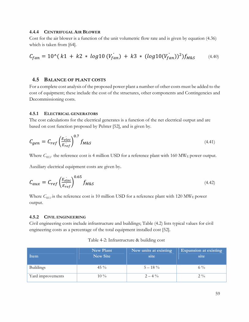
59

4.4.4 CENTRIFUGAL AIR BLOWER Cost for the air blower is a function of the unit volumetric flow rate and is given by equation (4.36) which is taken from [64]. = 10^( 1 + 2 ∗ 10 ( ) + 3 ∗ ( 10( )) ) & (4.40)

4.5 BALANCE OF PLANT COSTS For a complete cost analysis of the proposed power plant a number of other costs must be added to the cost of equipment; these include the cost of the structures, other components and Contingencies and Decommissioning costs.

4.5.1 ELECTRICAL GENERATORS The cost calculations for the electrical generates is a function of the net electrical output and are based on cost function proposed by Pelster [52], and is given by. = . & (4.41)

Where CREF the reference cost is 4 million USD for a reference plant with 160 MWE power output.

Auxiliary electrical equipment costs are given by.

= . & (4.42)

Where CREF is the reference cost is 10 million USD for a reference plant with 120 MWE power output.

4.5.2 CIVIL ENGINEERING Civil engineering costs include infrastructure and buildings; Table (4.2) lists typical values for civil engineering costs as a percentage of the total equipment installed cost [52].

Table 4-2: Infrastructure & building cost

Item

New Plant New Site

New units at existing site

Expansion at existing site

Buildings 45 % 5 – 18 % 6 %

Yard improvements 10 % 2 – 4 % 2 %

60

Table (4-2) leads to a simple way to calculate the Civil engineering costs which according to Pelster [52] can be misleading and will overestimate the cost estimation; for example the use of different technologies inside a gas turbine of a certain size will require the same Infrastructure with A similar gas turbine with the same size but not employing the same technologies or materials and so the cost can be estimated as a function of a the size the plant . For a combined cycle power plant the reference cost for civil engineering CREF, CIVIL = 66.9 million USD for reference power plant with a size of 226 MW.

, = . & (4.43)

4.5.3 NATURAL GAS SUBSTATION Natural gas delivered to the Integrated combined cycle power plant needs to be transported through a new pipeline connecting the plant with a gas main. According to Pelster [52] the cost function for the pipe branch is a function of the maximum flow rate of natural gas required by the power plant and is given by.

= ,. + & (4.43)

Where and are 219,000 USD and 221,000 USD respectively. A station for reducing pressure is required to lower the pressure from the pipeline pressure (~ 70 Bar) to the combustor pressure; the cost is also a function of the gas flow rate and is given by.

= ,. & (4.44)

4.5.4 CONTINGENCIES AND DECOMMISSIONING Unexpected costs related to technical and regulatory difficulties must be taken into account, according to the international energy agency [65] a typical contingency cost for combined cycle power plant is 5 % of investment costs. In the case of new technologies such as ISCC or first of a kind concepts a higher contingency cost can be assumed which is 10 % of investment costs.

When the plant reach the end of its useful lifetime, the equipment must be dismantled and the site restored to the original state, in the case of combined cycle power plants the decommissioning costs can be assumed to be equal to the salvage value of the equipment ( e.g. scrap metal value , carbon permits . etc). Since the share of the solar part of the power plant is relatively small comparing to the gas fired combined cycle a net zero costs for decommission will be assumed [65].

61

4.6 INTEGRATED SOLAR COMBINED CYCLE TOTAL INVESTMENT The total investment cost of the plant is then the sum of the costs of the three sub cycles and the balance of plant components.

, = , + , + , + , (4.45)

4.7 OPERATION AND MAINTENANCE COST

4.7.1 FUEL AND WATER COST The cost of fuel represents the highest share in O&M costs which depends on the price of the fuel as well on the amount of fuel burned annually; the price of natural gas depends on prices in the world market. Currently the price of natural gas in importing European countries is around USD 10.5/MMBtu [53]. Different fuel prices and their effect on LCOE will be studies later on in the optimization section.

Water consumption is mainly attributed to mirror and compressor washing. For mirror washing the cost is a function of total mirror area and is given by. = (4.46)

Where = 50 / is a constant for typical water consumption in mirror washing according to data obtained from the US department of energy, Ch20 = 4 USD/1000Galons represents the Price of water for washing and cooling in dry areas for combined cycle power plants [55].

As for compressor washing the cost function is derived from figures of an online washing technique [66] and is given by. = + (4.47)

Where & are 90 lith2o and 0.5 lith2o /(kg/s) respectively , based on data obtained from [66], MA is the mass flow through the compressor and f wash is the washing frequency of the equipment which is taken as once per day for each day of plant operation.

4.7.2 SPARE PARTS AND REPAIRS Costs for repairs and spare parts are taken as a percentage of the total equipment costs, building and other civil engineering component are assumed to have 1%/yr service charge, the gas turbine cycle components at of 2 %/yr , for the Heliostat field due to high probability of mirror breakage a value of 3 % / yr and for solar receiver , gas piping a value of 4 % /yr is assumed to harsh conditions met by these components such as high temperatures.

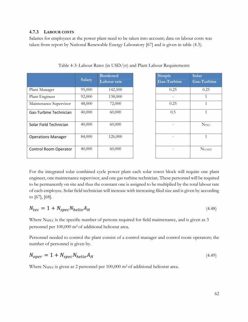
62

4.7.3 LABOUR COSTS Salaries for employees at the power plant need to be taken into account; data on labour costs was taken from report by National Renewable Energy Laboratory [67] and is given in table (4.3).

Table 4-3: Labour Rates (in USD/yr) and Plant Labour Requirements

Salary

Burdened Labour rate

Simple Gas-Turbine

Solar Gas-Turbine

Plant Manager 95,000 142,500 0.25 0.25

Plant Engineer 92,000 138,000 - 1

Maintenance Supervisor 48,000 72,000 0.25 1

Gas‐Turbine Technician  

40,000 60,000 0.5 1

Solar Field Technician  

40,000 60,000 - NTEC

Operations Manager  

84,000 126,000 - 1

Control Room Operator  

40,000 60,000 - NCONT

For the integrated solar combined cycle power plant each solar tower block will require one plant engineer, one maintenance supervisor, and one gas turbine technician. These personnel will be required to be permanently on site and thus the constant one is assigned to be multiplied by the total labour rate of each employee. Solar field technician will increase with increasing filed size and is given by according to [67], [68]. = 1 + (4.48)

Where NSPEC is the specific number of persons required for field maintenance, and is given as 3

personnel per 100,000 m2 of additional heliostat area.

Personnel needed to control the plant consist of a control manager and control room operators; the number of personnel is given by. = 1 + (4.49)

Where NSPEC is given as 2 personnel per 100,000 m2 of additional heliostat area.

63

4.7.4 SERVICE CONTRACTS For solar thermal power plants three service contracts are usually necessary [67] which are: Ground keeping and mirror washing and field control systems.

Field control systems are given as a fixed value of 100,000 USD, where for ground keeping and mirror washing are given by. = 100,000. .

(4.50) = 350,000. (4.51)

4.8 PERFORMANCE INDICATORS Alongside the LCOE other important figures of merit can be calculated with the use of the total costs of the plant and the net energy produced.

4.8.1 SOLAR SHARE The solar share ( fSOL) is an indicator to measure the percentage of the heat input the solar component contribute to the ISCC and is given by. = (4.52)

Where QSOL is the heat input of the solar circuit into the cycle and QFUEL is the heat input from the combustion chamber. These values were obtained after running the simulation for one year.

4.8.2 CARBON DIOXIDE EMISSIONS Reducing carbon emissions is a benefit of adding a solar component to the combined cycle, by increasing the solar share of the power plant the amount of fuel burned will be reduced and thus carbon emissions to the environment in reduced, furthermore the financial benefits of reducing the cost of carbon emissions increases as the mass of CO2 rejected per KWh is reduced. It is assumed that the natural gas fuel consists of pure methane, the chemical reaction of burning the fuel is given by. 4 + 3 2 → 2 + 2 2 (4.53)

The mass of CO2 rejected is given by.

64

= . ,, (4.54)

Where MFUEL,NET annual amount of fuel burned in Kg and PFUEL,NET is the annual power output.

4.8.3 POWER PLANT FUEL EFFICIENCY The overall efficiency of the power plant is based on the ratio of the produced power to the total fuel input, and is given by: = , (4.55)

4.9 DATA TRANSFER FROM TRNSYS The previous performance indicators and the component cost functions are written into MATLAB functions, in order to obtain the required yearly values such as the yearly total electricity output and the total mass of fuel consumed, data is exported from TRNSYS through type 65 printer component for each time step into a TXT file, afterwards the data file is imported in MATLAB and summation is applied to obtain yearly values before assigning to the functions.

65

5 OPTIMIZATIONOFTHEINTEGRATEDSOLARCOMBINEDCYCLEThis chapter introduces a brief description of the multi objective optimization concept, followed by a detailed description of the integration of the TRNSYS model within a multi-objective optimization program in order to find the most feasible plant setup. Objective functions and boundary conditions for the optimization process will also be described.

5.1 MULTI-OBJECTIVE OPTIMIZATION The process of simultaneously optimizing two or more objectives is called multi objective optimization (MOO). The optimization process is governed by a number of constraints, these constraints plus the objectives are functions of the decision variables. Multi objective optimization can be used in many fields to maximize profit, minimize cost and numerous other complex problems. In this work multi objective optimization will be applied to selected objective functions such as the Levelized cost of electricity and solar share or carbon dioxide emissions and solar share. In the following sections a brief introduction of the multi objective optimization followed by the selection of objective value and decision variables is given.

The mathematical definition of a multi objective optimization problem can be described as follows [69].

Maximize = ( ) = [ ( ), ( ), … , ( )] (5.1)

Subject to ( ) ≤ 0 , = 1, … … … . . = ( , , … … . ) ∈ = ( , , … … . ) ∈

Where k is the objective functions, x and y is the decision and objective vectors respectively, X and Y are the decision and objective spaces, respectively.

A unique solution to the optimization problem that satisfies all objectives cannot be found due to the nature of the conflicting objectives, one example can be made when the solar share of the power plant and the investment cost are chosen as objective functions, we would like to maximize the solar share of the plant and minimize the investment cost function. This requires us to increase the relatively expensive solar components leading to an increase in the second objective, thus we cannot increase the solar share without also increasing the investment cost.

There exist several approaches to obtaining solutions for multi objective optimization problems such as combing all the objective functions into a single objective function ,one example is the enviro -economic

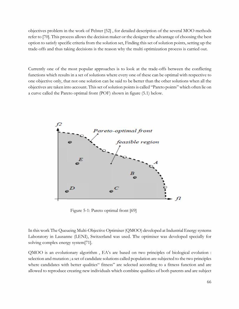
objectiverefer to [7option totrade-offs

Currentlyfunctionsone objecobjectivea curve ca

In this woLaboratosolving co

QMOO selection where canallowed to

s problem in70]. This proc satisfy specis and thus ta

y one of the s which resultctive only, ths are taken inalled the Pare

ork The Queury in Lausanomplex energ

is an evolutiand mutationndidates witho reproduce

n the work ofcess allows thfic criteria froking decision

most popults in a set of sat not one so

nto account. Teto optimal f

Figure 5-1:

ueing Multi-Onne (LENI), gy system[71

ionary algorin ; a set of canh better qualcreating new

f Pelster [52]he decision mom the solutins is the reas

ar approachesolutions wholution can bThis set of sofront (POF)

: Pareto optim

Objective OpSwitzerland

1].

ithm , EA’s ndidate solutilities“ fitness

w individuals w

, for detailedmaker or the dion set, Findion why the m

es is to lookhere every onebe said to be bolution pointsshown in fig

mal front [69

ptimiser (QMOwas used. T

are based oions called pos” are selectewhich combi

d descriptiondesigner the aing this set ofmulti optimiz

k at the tradee of these canbetter than ths is called “Pagure (5.1) belo

9]

OO) developThe optimise

n two princiopulation areed accordingine qualities o

n of the severadvantage off solution poization proces

e-offs betwen be optimal he other soluareto points” ow.

ped at Industrer was develo

iples of biole subjected tog to a fitnessof both paren

ral MOO mef choosing theints, setting uss is carried o

en the conflwith respect

utions when awhich often

rial Energy syoped speciall

logical evolu the two prin

s function annts and are su

66

thods e best up the out.

licting tive to all the lie on

ystems ly for

ution : nciples nd are ubject

67

to random mutation resulting in new candidates competing with the parents to be in the next generation. EA are highly suitable for solving multi objective optimization problems due to the ability to acquire numerous Pareto-optimal solutions in a single simulation run[69].

The algorithm of the QMOO can be described in six steps as follows [71]:

Creation: New individuals are created and stored in the queue for assignment.

Assignment: The individual is removed from the queue and assigned a set of parameter values; the assignment parameters are selected at random when the algorithm is still initializing or by applying mutation and reproduction operator when the initialization process is finished.

Evaluation: Objective functions area evaluated and the individual is queued for grouping or ranking.

Grouping: The individual is assigned to a group to be ranked.

Ranking: Individuals are ranked and given permission as parents to reproduce.

Removal: Individuals are finally removed from the group if their fitness does not meet specific requirements.

The QMOO is integrated into the MATLAB environment. It is connected to another toolbox, called OSMOSE (A tool for design and analysis of integrated energy systems) developed at LENI. That handles and organizes the computation of the MOO.

68

5.2 THE OPTIMIZATION PROCEDURE The optimization program follows a black box approach. Figure (5.2) shows a simplified data flow of the program.

The optimizer block consists of a numerous Matlab functions; however the user need only modify two functions for the optimization process to start. The first function frontend_ISCC is where all the optimization specifications are modified, population size is chosen first, a value of 32 is taken and the population cluster is set to one, afterwards the number of objective functions is entered with the option to either be maximized or minimized during the optimization, following this the number of decision variables and their limits is set, finally the number and values of the optimization constants is specified. The second function in the optimizer that needs to be modified by the user is osmoseInterface which provides the interface between the optimizer and the ISCC Matlab function, osmoseInterface receives the decision variables from the frontend_ISCC and passes them to MOO, and then the optimizer assigns values to the decision variable for the first evaluation set and passes them back to osmoseInterface which creates an input vector containing the decision variables from MOO and passes them on to ISCC function. Now the TRNSYS model is called and the results of the simulation are imported back into ISCC for calculation of the objective functions and the performance parameters. Afterwards ISCC passes these parameters back to osmoseInterface. Now the objective functions are passed on to MOO where the optimization commences once the population size is created.

TRNSYS Model Simulation

ISCC MATLAB Model

Optimizer

Decision variables Objective functions

Simulation parameters Simulation results

Figure 5-2: Optimization data flow

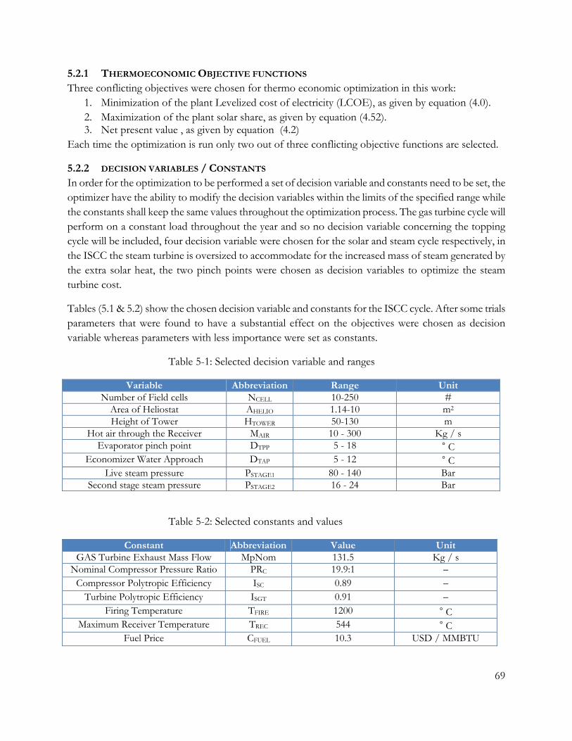
69

5.2.1 THERMOECONOMIC OBJECTIVE FUNCTIONS Three conflicting objectives were chosen for thermo economic optimization in this work:

1. Minimization of the plant Levelized cost of electricity (LCOE), as given by equation (4.0). 2. Maximization of the plant solar share, as given by equation (4.52). 3. Net present value , as given by equation (4.2)

Each time the optimization is run only two out of three conflicting objective functions are selected.

5.2.2 DECISION VARIABLES / CONSTANTS In order for the optimization to be performed a set of decision variable and constants need to be set, the optimizer have the ability to modify the decision variables within the limits of the specified range while the constants shall keep the same values throughout the optimization process. The gas turbine cycle will perform on a constant load throughout the year and so no decision variable concerning the topping cycle will be included, four decision variable were chosen for the solar and steam cycle respectively, in the ISCC the steam turbine is oversized to accommodate for the increased mass of steam generated by the extra solar heat, the two pinch points were chosen as decision variables to optimize the steam turbine cost.

Tables (5.1 & 5.2) show the chosen decision variable and constants for the ISCC cycle. After some trials parameters that were found to have a substantial effect on the objectives were chosen as decision variable whereas parameters with less importance were set as constants.

Table 5-1: Selected decision variable and ranges

Variable Abbreviation Range Unit Number of Field cells NCELL 10-250 #

Area of Heliostat AHELIO 1.14-10 m2 Height of Tower HTOWER 50-130 m

Hot air through the Receiver MAIR 10 - 300 Kg / s Evaporator pinch point DTPP 5 - 18 ° C

Economizer Water Approach DTAP 5 - 12 ° C Live steam pressure PSTAGE1 80 - 140 Bar

Second stage steam pressure PSTAGE2 16 - 24 Bar

Table 5-2: Selected constants and values

Constant Abbreviation Value Unit GAS Turbine Exhaust Mass Flow MpNom 131.5 Kg / s

Nominal Compressor Pressure Ratio PRC 19.9:1 - Compressor Polytropic Efficiency ISC 0.89 -

Turbine Polytropic Efficiency ISGT 0.91 - Firing Temperature TFIRE 1200 ° C

Maximum Receiver Temperature TREC 544 ° C Fuel Price CFUEL 10.3 USD / MMBTU

6

In this seimportanthe solar carbon ta

The optimoptimizatfurther eva minimuprogressiallowed t

In this wCalifornia

OPTIMIZA

ection the resnt trade off cu

share and thax will be eva

mization is alltion is terminvaluations wium of 1000 iton of the opto run for a s

work the sima (2,792 KW

ATIONRE

sults of the ourves are studhe carbon dioaluated.

lowed to runnated when tll not extend terations to atimization prufficient num

Fig

mulations werWh / m2/ yr) a

ESULTS&

optimization died such as: toxide emissio

until a smoothe points at the curve mu

a maximum orocess; a well-mber of evalu

gure 6-1: Typ

re conductedand one site w

DISCUSSI

for the objecthe investmenons. Further

oth and continthe end of t

uch. In this wof 4000 iterat-defined Pareuations.

pical POF cu

d for two lowith medium

ON

ctive functiont cost and thrmore the eff

nuous Paretothe curve are

work the optimtions. Figure eto curve is e

urve

ocations, onem to high DN

ons is detailedhe Levelized fect of varyin

o-front curvee in very closmization was (6.1) shows stablished aft

e with high NI level, Paler

d, moreover cost of electrng fuel price

e is establishese value rangallowed to ruan example oter the optimi

DNI, Daggrmo in Italy

70

other ricity , es and

ed, the ge and un for of the izer is

gett in (1850

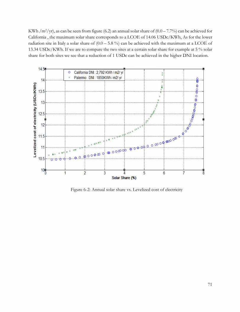
KWh /mCaliforniaradiation 13.34 USshare for

m2/yr), as can a , the maximsite in Italy aDc/KWh. Ifboth sites w

be seen frommum solar shaa solar share f we are to co

we see that a r

Figure 6-2:

m figure (6.2) are corresponof (0.0 – 5.8

ompare the twreduction of

: Annual sola

an annual solnds to a LCO8 %) can be awo sites at a c1 USDc can

ar share vs. L

lar share of (0OE of 14.06 Uachieved withcertain solar be achieved

Levelized cos

0.0 – 7.7%) cUSDc/KWhh the maximshare for exa

d in the highe

st of electricit

can be achieveh, As for the l

mum at a LCOample at 5 %er DNI locati

ty

71

ed for lower

OE of % solar

ion.

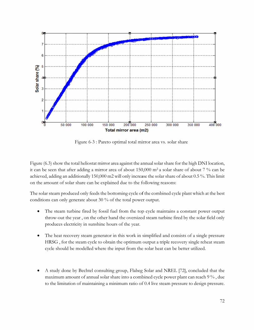
Figure (6.it can be achieved,on the am

The solarcondition

Tthp

THcy

Amto

.3) show the tseen that aft

, adding an admount of sola

r steam produns can only g

The steam turhrow-out theroduces elect

The heat recoHRSG , for thycle should b

A study done maximum amo the limitatio

Figure 6-3

total heliostater adding a mdditionally 15ar share can b

uced only feeenerate abou

rbine fired be year , on thetricity in sun

overy steam ghe steam cyclbe modelled w

by Bechtel count of annuon of mainta

: Pareto opti

at mirror area mirror area o50,000 m2 wibe explained

eds the bottomut 30 % of th

y fossil fuel e other hand shine hours

generator in te to obtain thwhere the inp

consulting grual solar shareining a minim

imal total mi

against the anof about 150ill only increa due to the f

ming cycle ofhe total powe

from the topthe oversizedof the year.

this work in she optimum put from the

roup, Flabege into a combmum ratio of

irror area vs.

nnual solar sh0,000 m2 a soase the solar sfollowing rea

f the combineer output.

p cycle maintd steam turb

simplified anoutput a trip

e solar heat c

g Solar and Nbined cycle pf 0.4 live stea

solar share

hare for the holar share of share of abouasons:

ed cycle plan

tains a constbine fired by t

nd consists ople recovery scan be better

NREL [72], cpower plant cam pressure t

high DNI locabout 7 % c

ut 0.5 %. This

nt which at th

tant power othe solar field

f a single preingle reheat sutilized.

concluded thaan reach 9 %

to design pre

72

ation, can be s limit

e best

output d only

essure steam

at the % , due

ssure.

Tthth

To see atsolar sharelectricitycalculate solar onlyFeed-in-t

This agrees wihat is due to through.

t what solar sre for the higy, statistical dthe benefits y share of thtariff scheme

ith Figure (6.the turbine be

Figure 6-4:

shares the prgh DNI case. data for the Sresulting froe electricity a was adapted

.4) we see thaeing too large

: Live Steam

roject is deemin order to c

Spanish markm the sale ofa value of 0.3d[74].

at the steam pe for the heat

pressure of R

med profitablcorrectly calcket electricityf the fossil fu35 USDc /K

pressure durit input when t

Rankine cycl

le or not, theculate the beny pool pricesuel electricity

KWh (0.28 €c

ing non-solarthe hot air is

le at 6 % sola

e NPV is evanefits resultins in the year y share of thec/KWh) from

r hour’s dropnot being pum

ar share

aluated againng from the s2008 was us

e plant[73], fom the late Sp

73

ps and mped

nst the sale of sed to or the panish

The NPVconsideremade.

The upfrpower tecinvestmenincreasedjustify theinvestmen

V in figure (6ed and thus so

ont investmechnology, in ant cost must

d efficiency ane investment nt cost for th

Fig

6.5) is positivolar shares be

ent cost is thaddition to thbe studied; innd reduced Ccosts. Figure

he two sites.

gure 6-5: Ann

ve above a soelow 3.5 are d

he most impohe Levelized ntroducing soCO2 emissione (6.6) shows

nual Solar sh

olar share valdeemed unfea

ortant barriecost of energolar power tons although itthe progressi

hare vs.NPV

lue of 3.5 %asible against

er to the pengy the effect oo the combinet must be ecoion of the ann

, negative NPthe amount o

netration of cof increased sed cycle has aonomically fnual solar sha

PV should nof new invest

concentrated solar share onadvantages sufeasible in ordare versus the

74

not be tment

solar n total uch as der to e total

At zero soMillion Uexponentabove a vcosts of thalso showMillion Unecessary

olar shares thUSD, the tottially, as with value of abouthe solar cycle

w that for theUSD comparey to achieve t

Figure 6-6:

he total investal cost initialthe solar shat 7.7 % for the componente same solar sed to 147 Mithe same pow

: Annual sola

tment cost is lly increases

are limit in Fighe California ts, but also foshare (e.g.: 5 illion USD fower output pe

ar share vs. T

equal to the linearly with

gure (6.2) thesite. The incr

or the increase%) the site w

or the site in ercentage wh

Total equipm

cost of a comh the increase limit of the rease in total ed size of thewith high DNItaly, this is d

hen the DNI

ment cost

mbined cycle psing solar shasolar share cacost is mainl

e steam turbinNI will have due to the in is lower.

power plant aare and thenannot be incrly due to the ane unit, the ga total cost o

ncreased solar

75

at 100 n rises reased added

graphs of 120 r field

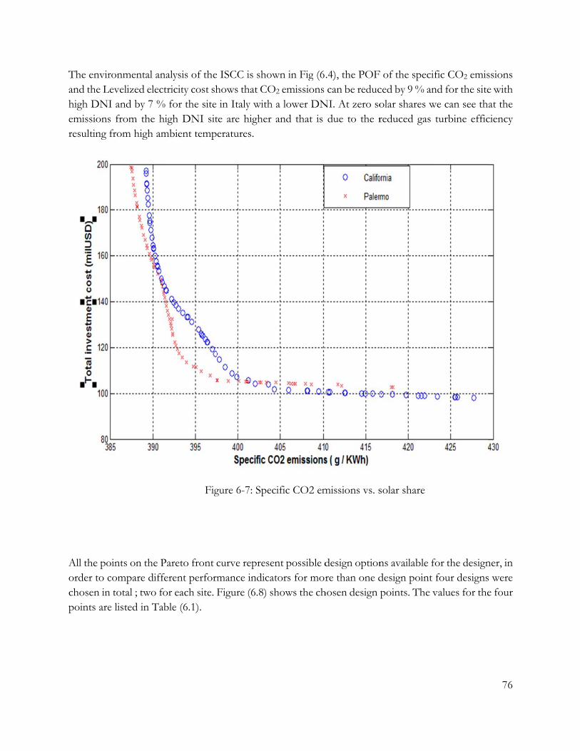
The envirand the Lhigh DNemissionsresulting

All the poorder to cchosen inpoints are

ronmental anLevelized elecI and by 7 %s from the hfrom high am

oints on the Pcompare diffn total ; two fe listed in Ta

nalysis of thectricity cost sh% for the site high DNI sitmbient temp

Fig

Pareto front cferent performfor each site. Fable (6.1).

ISCC is shohows that COin Italy with

te are highereratures.

gure 6-7: Spe

curve represemance indicaFigure (6.8) s

own in Fig (6O2 emissions h a lower DNr and that is

cific CO2 em

ent possible dators for morshows the ch

.4), the POFcan be reduc

NI. At zero sodue to the r

missions vs. s

design optionre than one d

hosen design

F of the speciced by 9 % anolar shares wreduced gas

solar share

ns available fdesign point points. The v

fic CO2 emisnd for the sitewe can see th

turbine effic

for the designfour designsvalues for the

76

ssions e with at the ciency

ner, in s were e four

IndiLC

SolarCombin

EfficMaximu

OuAnnual pTotal In

Specific i

Number oTotal m

Tower

dicator COE r share ned cycle ciency um Plant utput production nvestment nvestment

of heliostats mirror area r Height

Figure 6-8:

Table 6-1:

Californ

Point 1 10.8 7.0 52.5

63.03

552 141.7 2248

29500 157080

96

: Selected de

Selected poin

nia Site

Point 214.1 7.65 54.5

66

571.2 197.552993

353160353160

130

sign points o

nt’s characte

Pale

Point 112.9 5.0 48

61.8

541.2 129.2 2090

113640113640

104

on the POF

eristics

ermo Site

Point 214.25.950

64.5

566.91963038

356320356320

130

2 UUSDc

M

GWMillioUSD

0 0 m

Units c/KWhe % %

MWe

Whe on USD / KWe

# m2 m

77

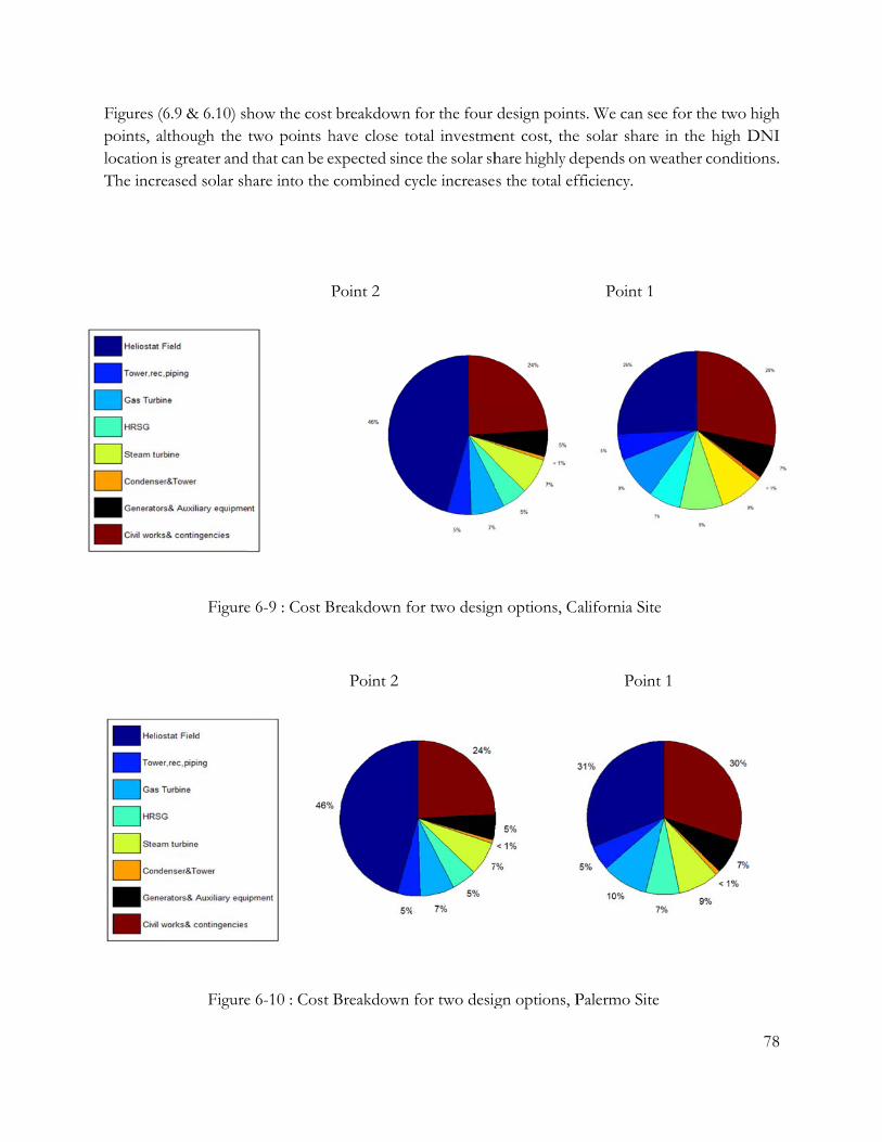
Figures (6points, allocation iThe incre

6.9 & 6.10) shlthough the s greater and

eased solar sh

Figure

Figure

how the costtwo points h

d that can be ehare into the

e 6-9 : Cost B

e 6-10 : Cost

t breakdown have close toexpected sinccombined cy

Point 2

Breakdown fo

Point 2

Breakdown

for the four otal investmece the solar shycle increase

or two design

for two desig

design pointent cost, thehare highly ds the total ef

n options, C

gn options, P

ts. We can see solar share depends on wfficiency.

Point 1

alifornia Site

Point

Palermo Site

ee for the twoin the high

weather condi

e

t 1

78

o high DNI

itions.

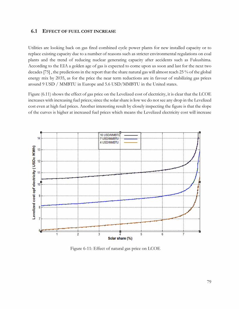
6.1 E

Utilities areplace explants anAccordindecades [energy maround 9

Figure (6.increases cost evenof the cur

EFFECT OF

are looking bxisting capacind the trend ng to the EIA75] , the pred

mix by 2035, USD / MM

.11) shows thwith increasi

n at high fuel rves is higher

F FUEL COS

back on gas fity due to a nof reducing

A a golden agdictions in theas for the pr

MBTU in Euro

he effect of ging fuel priceprices. Anothr at increased

Figure 6-11

ST INCREAS

fired combinnumber of reag nuclear gee of gas is exe report that trice the near ope and 5.6 U

gas price on thes; since the sher interestind fuel prices w

1: Effect of n

SE

ned cycle powasons such asnerating cap

xpected to cothe share natterm reduct

USD/MMBT

he Levelized olar share is lng result by cwhich means

natural gas pr

wer plants fos stricter envipacity after aome upon us tural gas will ations are in fTU in the Un

cost of electlow we do no

closely inspecs the Leveliz

rice on LCO

or new instalvironmental raccidents sucsoon and las

almost reach favour of stanited states.

tricity, it is cleot see any drocting the figuzed electricity

OE

lled capacity regulations onch as Fukusst for the nex25 % of the gbilizing gas p

ear that the Lop in the Levere is that the

y cost will inc

79

or to n coal hima.

xt two global prices

LCOE elized slope

crease

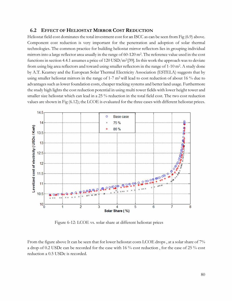
6.2 EHeliostat Componetechnologmirrors infunctionsfrom usinby A.T. Kusing smaadvantagethe study smaller sivalues are

From thea drop ofreduction

EFFECT OF

field cost doent cost redgies. The comnto a large refs in section 4.ng big area reKearney and aller heliostates such as lowhigh lights th

ize heliostat we shown in Fi

Figure

e figure abovef 0.2 USDc cn a 0.5 USDc

F HELIOSTA

ominates the tduction is vemmon practicflector area u.4.1 assumes flectors and tthe Europeat mirrors in t

wer foundatiohe cost reducwhich can leaig (6.12); the

e 6-12: LCOE

e It can be sean be record

c is recorded.

AT MIRRO

total investmery importance for buildin

usually in the ra price of 120toward usingn Solar Therthe range of on costs, cheaction potentiaad in a 25 % rLCOE is eva

E vs. solar sh

en that for loded for the ca

OR COST RE

ent cost for ant for the peng heliostat mrange of 60-10 USD/m2 [3

g smaller reflermal Electrici1-7 m2 will leaper tracking al in using mureduction in aluated for th

hare at differ

ower heliostatase with 16 %

EDUCTION

an ISCC as caenetration anmirror reflect120 m2. The r39]. In this woectors in the rity Associatioead to cost resystems and

ulti tower fielthe total field

he three cases

ent heliostat

t costs LCOE% cost reduct

N an be seen frond adoption tors lies in grreference valuork the approrange of 1-10on (ESTELAeduction of abetter land ulds with lowed cost. The tws with differe

prices

E drops , at ation , for the

om Fig (6.9) aof solar th

rouping indivue used in th

oach was to de0 m2. A studyA) suggests thabout 16 % dusage. Furtherer height towetwo cost redunt heliostat p

a solar share ocase of 25 %

80

above. ermal vidual e cost eviate

y done hat by due to rmore er and uction prices.

of 7% % cost

81

7 CONCLUSIONSANDFUTUREWORK

The first part of the study concluded that central receiver tower systems working with atmospheric air as a HTF fluid are a suitable option for integrating concentrating solar power into conventional power cycles. The simplicity, safe operation and predicted cost reduction gives this technology an edge over the existing CSP technologies.

A model of the Integrated Solar combined cycle was created in the simulation software TRNSYS, transient simulation covering the performance for a complete year was evaluated, t weather data for the two locations were generated by the software Meteonorm, the data contains hourly values of solar radiation and metrological data, the model can be tested for different locations by simply changing the weather data file and update the heliostat field efficiency matrix function in MATLAB.

The thermo economic optimization was done by suing an evolutionary multi objective optimiser in MATLAB. The results of the investigated model show that an annual solar share of about 5, 7 % can be achieved in low, high DNI locations respectively. These results show reasonable values when compared with solar share values (around 4 %) from recently built ISCC plants in Egypt and Morocco[76]. The limited solar shares is attributed to limitations in the oversized steam cycle, first the increased amount of steam generated in the unit cannot go above a certain limit, second the heat input to the cycle in non-solar hours is too low to produce the design live steam pressure resulting in a pressure drop reaching in some designs to almost 50 %.

Reduction of CO2 emissions in the ISCC is small; by increasing the total power output of the plant the carbon emissions can be reduced relatively (compared to the same power output from a complete fossil fired plant which burn fuel to achieve the same increased output), although the reduced share is small it can amount to a significant reduction if the cycle size was increased.

The economic analysis showed that the Levelized cost of electricity to be in the range of 10.5-14 USDc/ KWh, comparing these values with CSP only plant having LCOE in the range of 15-20 USDc/KWh [29],[39] shows that ISCCS offers attractive and favourable levelized electricity costs . It should be noted though for a thorough comparison the two different plants should have the same conditions (DNI, Capacity ...etc) but the values in general show that for ISCC generation costs are lower. NPV analysis showed that for a positive return on the solar investment a minimum solar share of 3.5 % and maximum of 7.2 % should be followed in the design.

The result from this study show the potential of integrating atmospheric central receiver tower into combined cycle power plants, for future work a number of measures can be implemented to further improve the design:

A better design for the air circuit should be studied, the mixture of flue gasses and hot air should be pumped back to the solar receiver raising the efficiency and resulting in a more stable

82

operation since the receiver will be able to maintain the maximum temperature for a longer period of time.

The HRSG in the steam cycle should be simulated for two pressure levels instead of one in order to better use the exhaust heat; furthermore a single reheat steam cycle can be modelled thus further increasing the efficiency.

Different sizes of the combined cycle should be studies to find the most economical designs.

The simulations show that ISCC are a low cost, highly dispatchable source of power, even though only small amount of solar share can be incorporated (3.5 % - 7 %), the potential of deploying this technology in all newly built combined cycle plants should lead to an important amount of reduced emissions, drive for cost reduction for the solar components and job creation. the green message the ISCC can pave the way for wider acceptance of renewable energy sources on a big scale.

83

8 BIBLIOGRAPHY[1] Natalia Kulichenko and Jens Wirth, "Regulatory and Financial Incentives for Scaling Up

Concentrating Solar Power in Developing Countries," Washington, DC, 2011.

[2] Ausra. (2010, January ) Solar Steam Boosters for Coal-fired Power Plants.. [Online]. www.ausra.com

[3] TRNSYS, "TRNSYS – A Transient System Simulation Program," Madison, Wisconsin, 2006.

[4] John Duffie and William Beckman, Solar Engineering of Thermal Processes, Third Edition. New Jersey: John Wiley & Sons, 2006.

[5] M Romero, Martinez D, and Zarza E, "Terrestrial solar thermal power plants: on the verge of

commercialization," in 4th int conf on sol power from space, 2004.

[6] Robert Pitz-Paal. (2007) http://www.nrel.gov. [Online]. http://www.nrel.gov/csp/troughnet/pdfs/2007/pitz_paal_dlr_solar_resource_assessment.pdf

[7] DLR, "Concentrating Solar Power for the Mediterranean Region ," Stuttgart, 2005.

[8] A Rabl, "Comparison of solar concentrators," Solar energy, p. pp.93, 1976a.

[9] R Pitz-Paal, "High Temperature Solar Concentrators Solar Energy Conversion and PhotoenergySystems.In Encyclopedia of Life Support Systems," in Future Energy - Improved, Sustainable and Clean Options for Our Planet. Oxford: Eolss Publishers, 2008, pp. 171-191.

[10] Yogi Goswami and Frank Kreith, Energy Conversion.: CRC Press, 2007.

[11] Samuel Roy. (1998) compeduhpt. [Online].

http://www.energy.kth.se/compedu/Compedu_home_asp/main/default.asp

[12] Rolf Kehlhofer, Bert Rukes, Frank Hannemann, and Franz Stirnimann,

Combined - Cycle Gas & Steam Turbine Power Plants. Tulsa: PennWell Corp, 2009.

[13] Enea. (2011) ENEA. [Online]. http://www.enea.it

[14] E Zarza , "Generacion directa de vapor con Colectores solares cilindro para parabolicos

proyecto Direct Solar Steam (DISS). ," Madrid, 2004.

84

[15] Wikipedia. (2012, Feb.) Wikipedia. [Online]. http://en.wikipedia.org

[16] DLR. (2012) dlr.de/media. [Online]. http://www.dlr.de/media/desktopdefault.aspx/tabid-4984/

[17] Soteris A Kalogirou, Solar Energy Engineering - Processes and Systems. California: Academic Press, 2009.

[18] NOVATEC. (2011) novatecsolar.com. [Online]. http://www.novatecsolar.com;

[19] DAVID R MILLS and GRAHAM L MORRISON, "COMPACT LINEAR FRESNEL REFLECTOR SOLAR THERMAL POWER PLANTS," Solar Energy Vol. 68, No. 3, pp. 263–283, 2000.

[20] Bernhard et al, "Linear Fresnel Collector demonstration at the PSA – operation and investigation.," in 15th International SolarPACES Symposium, Berlin, Germany., 2009.

[21] Abengoa. (2011) http://www.abengoasolar.com. [Online]. http://www.abengoasolar.com/corp/web/en/nuestras_plantas/plantas_en_operacion/espana/PS20_la_mayor_torre_comercial_del_mundo.html.

[22] Tyner et al, "Solar Two: A Molten Salt Power Tower Demonstration," Albuquerque, 1995.

[23] M Schmitz-Goeb and G Keintzel, "The Phoebus Solar Power Tower," in ASME Int. Solar Energy Conf, Washington D.C., 1997, pp. pp. 47–53.

[24] Heller et al, "Test and evaluation of a solar powered gas turbine system," Solar Energy,Vol 80 ,

Issue 10, pp. 1225-1230, 2006.

[25] Schwarzbo¨zl et al, "Solar gas turbine systems: Design, cost and perspectives," Solar Energy Vol.80, pp. 1231–1240, 2006.

[26]

Solarpaces. (2010) solarpaces.org. [Online].

http://www.solarpaces.org/CSP_Technology/csp_technology.htm

[27] W.B. Stine and R.P Diver,"A Compendium of Solar Dish/Stirling Technology,"Albuquerque, 1994.

85

[28] D.R Gallup and J.B Kesseli, "A Solarized Brayton Engine Based on Turbo-Charger Technology

and the DLR Receiver," in IECEC, AIAA-94-3945-CP, Monterey, CA, 1994.

[29] IEA, "Technology Roadmap Concentrating solar power," Paris, 2010.

[30] Trieb et al, "SOLAR ELECTRICITY GENERATION- A COMPARATIVE VIEW OF TECHNOLOGIES , COSTS AND ENVIRONMENTAL IMPACT," Solar energy vol.59, pp. 89-99, 1997.

[31] Farid bensebaa, "Solar based large scale power plants: what is the best option?," PROGRESS IN PHOTOVOLTAICS: RESEARCH AND APPLICATIONS, pp. 240-246, 2011.

[32] Brighsource Energy inc. (2011, October) Brighsource Energy. [Online]. www.brightsourceenergy.com

[33] Fichtner, "Technology Assessment of Concentrated Solar Thermal Power Technologies for a Site Specific Project in South Africa," 2010.

[34] C TURCHI, M MEHOS, C. K HO, and G. J KOLB, "Current and future costs for

parabolic trough and power tower systems in the US market.," in SolarPACES 2010., Perpignan ,France, 2010.

[35] M Geyer, "Geyer M. Introducing concentrated solar power on the international market-

worldwide incentives, policies and benefits," in SolarPACES 2008, 14th int symp on conc sol power

and chem energy technology, Las Vegas, 2008.

[36] Sargent & Lundy LLC Consulting Group, "Assessment of Parabolic Trough and Power Tower Solar Technology Cost and Performance Forecasts," Chicago, Illinois, 2003.

[37] Viebahn Peter, Kronshage Stefan, and Franz Trieb, "New Energy Externalities Developments for Sustainability ( NEEDS)," 2008.

[38] Craig E Tyner and James E Pacheco, "eSolar’s POWER PLANT ARCHITECTURE," California, 2009.

[39] Sandia National Laboratories, "Power Tower Technology Roadmap and Cost Reduction Plan,"

Albuquerque, New Mexico, 2011.

86

[40] B Kelly, U Herrmann, and M.J Hale, "Optimization Studies for Integrated Solar

Combined Cycle Systems," in Solar Forum 2001, Solar Energy: The Power to choose, Washington, DC, 2001.

[41] Peter Schwarzbözl and Deutsches Zentrum, A TRNSYS Model Library for Solar Thermal Electric

Components (STEC). Köln: DLR, 2006.

[42] Kolb et al., "Heliostat Cost Reduction Study," California, 2007.

[43] William B. Stine and Michael Geyer. (2001) Power from the sun chapter 10. [Online]. http://www.powerfromthesun.net/Book/chapter10/chapter10.html

[44] Incropera and DeWitt, Fundementals of Heat and Mass transfer.: Wiley and sons, 1996.

[45] ASHRAE, ASHRAE Handbook - Fundamentals.: American Society of Heating, Refrigerating and Air;, 2009.

[46] B Hoffschmidt, "Vergleichende Bewertung verschiedener Konzepte Volumetrischer Strahlungsempfanger," 1997.

[47] Antonio Avila Marin, "Volumetric receivers in Solar Thermal Power Plants with Central Receiver System technology: A review," Solar Energy, pp. 891-910, 2011.

[48] H P Garg, Advances in soalr energy technology. Dordrecht: D.Reidel, 1987.

[49] "SIEMENS SGT-800 INDUSTRIAL GAS TURBINE ENHANCED TO 47MW DESIGN MODIFICATIONS AND OPERATION EXPERIENCE," in Proceedings of ASME Turbo Expo 2008, Berlin, 2008.

[50] Magnus Holngren. (2006, Jan) X-eng. [Online]. www.X-eng.com

[51] P Walsh and P Fletcher, Gas Turbine performance, 2nd ed. Oxford: WileyBlackwell, 2004.

[52] Stefan Pelster, Environomic Modeling and Optimization of Advanced Combined Cycle Power Plants including CO2 Separation Options. Lausanne, Switzerland: Ecole Polytechnique Fédérale de Lausanne, 1998.

[53] Development Prospects Group. World Bank, "Commodity Price Forecast Update," 2012.

[54] IEA. (2011) IEA. [Online]. http://IEA.doe.gov/oiaf/aeo/electricity_generation.html

[55] John S. Maulbetsch and Michael N DiFilippo, "COST AND VALUE OF WATER USE AT

87

COMBINED-CYCLE POWER PLANTS," California, 2006.

[56] EUROPEAN COMMISION, "A Roadmap for moving to a competitive low carbon economy in 2050," Brussels, 2011.

[57] Wikipedia. (2012) Wikipedia. [Online]. http://en.wikipedia.org

[58] James Spelling, "Thermo-Economic Optimisation of Solar Tower Thermal Power Plants,"

Ecole Polytechnique Fédérale de Lausanne, Master Thesis 2009.

[59] C. A Frangopoulos, "Comparison of Thermoeconomic and Thermodynamic Optimal Designs of a Combined-Cycle Plant," in proceedings of the international conferenceon the Analysis ofThermal and Energy Systems, Athens, Athens, 1991.

[60] Chemical Engineering. (2011, DEC) CHE. [Online]. www.che.com

[61] B. L Kistler, "A User's Manual for DELSOL3 A Computer Code for Calculating the Optical

Performance and Optimal System Design for Solar Thermal Central Receiver Plants," California, 1986.

[62] S.A Gaznat, Personal communication, 1995.

[63] Wilfried Grasse, "PHOEBUS international 30MWe solar tower plant," Solar Energy Materials, pp. 82-94, 1991.

[64] R.K Turton, Principles of. Turbomachinery. London: Chapman and Hall, 1995.

[65] IEA and NEA, "Projected Costs of Generating Electricity," Paris, 2010.

[66] Friederike C. Mund and Pericles Pilidis, "Gas Turbine Compressor Washing: Historical Developments,

Trends and Main Design Parameters for Online Systems," Journal of Engineering for Gas Turbines and Power, pp. 344-353, 2006.

[67] C Turchi, "Parabolic Trough Reference Plant for Cost Modeling with the Solar Advisor Model," 2010.

[68] Robert Pitz-Paal, Jürgen Dersch, and Barbara Milow, "European Concentrated Solar Thermal Road-Mapping ( ECOSTAR)," 2003.

88

[69] Eckart Zitzler, Evolutionary Algorithms for Multiobjective Optimization:Multiobjective Optimization,Phd Thesis. Zurich: Swiss Federal Institute of Technology Zurich, 1999.

[70] R.T. Marler and J.S. Arora, "Survey of multi-objective optimization methods for engineering,"

Structural and Multidiciplinary Optimization , Volume 26, pp. 369-395, 2004.

[71] Geoffrey Basil Leyland, Multi-Objective Optimisation applied to Industrial Energy Problems. Lussane :

EPFL-STI, Laboratoire d’Energétique Industrielle, 2002.

[72] Bruce Kelly, Ulf Herrmann, and Mary Jane Hale, "Optimization Studies for Integrated Solar

Combined Cycle Systems," in ASME Forum 2001, 2001.

[73] omie. (2011) Operador del Mercado Ibérico de Energía. [Online]. http://www.omie.es

[74] CSP Today. (2011) csptoday. [Online]. www.csptoday.com (accessed 15th June 2012)

[75] IEA, "Golden Rules for a Golden Age of Gas," Paris, 2012.

[76] Abengoa Solar, "Experiences in developing , building and operating concentrating solar power plants," Melbourne, 2009.

[77] EPA. (2007) energystar.gov. [Online]. http://www.energystar.gov/index.cfm?c=business

[78] EIA, "Annual Energy Outlook 2010 with projections to 2035," Washington, 2010.

[79] AT Kearney and ESTELA, "Solar Thermal Electricity 2025 ,Clean electricity on demand: attractive STE cost stabilize energy production," 2010.

[80] Dersch et al, "Trough integration into power plants—a study on the performance and economy of integrated solar combined cycle systems," Energy, pp. 947–959, 2004.

89