Mobile Edge Computing Network Control: Tradeoff Between ...

arX

iv:2

005.

0785

4v2

[cs

.NI]

31

Jul 2

020

1

Mobile Edge Computing Network Control:

Tradeoff Between Delay and Cost

Yang Cai∗, Student Member, IEEE, Jaime Llorca†, Member, IEEE, Antonia M.

Tulino†‡, Fellow, IEEE, and Andreas F. Molisch∗, Fellow, IEEE

Abstract

As mobile edge computing (MEC) finds widespread use for relieving the computational burden of

compute- and interaction-intensive applications on end user devices, understanding the resulting delay

and cost performance is drawing significant attention. While most existing works focus on single-

task offloading in single-hop MEC networks, next generation applications (e.g., industrial automation,

augmented/virtual reality) require advance models and algorithms for dynamic configuration of multi-

task services over multi-hop MEC networks. In this work, we leverage recent advances in dynamic cloud

network control to provide a comprehensive study of the performance of multi-hop MEC networks,

addressing the key problems of multi-task offloading, timely packet scheduling, and joint computation

and communication resource allocation. We present a fully distributed algorithm based on Lyapunov

control theory that achieves throughput optimal performance with delay and cost guarantees. Simulation

results validate our theoretical analysis and provide insightful guidelines on overall system design and

the interplay between communication and computation resources.

I. INTRODUCTION

Resource- and interaction-intensive applications such as augmented reality, real-time computer

vision will increasingly dominate our daily lives [1]. Due to the limited computation capabilities

and restricted energy supply of end user equipments (UEs), many resource-demanding tasks that

cannot be executed locally end up being offloaded to centralized cloud data centers. However,

the additional delays incurred in routing data streams from UEs to distant clouds significantly

∗Y. Cai and A. F. Molisch are with University of Southern California, CA 90089, USA. (E-mail: [email protected],

[email protected]). †J. Llorca and A. M. Tulino are with Nokia Bell Labs, NJ 07733, USA. (E-mail: jaime.llorca@nokia-

bell-labs.com, [email protected]). ‡A. M. Tulino is also with Universitya degli Studi di Napoli Federico II, 80138

Naples, Italy. (E-mail: [email protected]).

August 3, 2020 DRAFT

http://arxiv.org/abs/2005.07854v2

2

Edge Cloud

Computing Server

Antennas

Wireless Links

(Directed Beams)

Wired Links

Core Cloud

UEs

… …

Fig. 1. An illustrative multi-hop MEC network consisting of UEs, edge cloud servers, and the core cloud. Edge servers

communicate with UEs via wireless links, and among each other and the core cloud via wired connections.

Video Source

(Input)Tracker

Overlay Image

(Output)

Object

Recognizer

Fig. 2. A function chain representation of an augmented reality service, composed of Tracker, Object Recognizer, and Renderer

functions [2].

degrade the performance of real-time interactive applications. To address this challenge, mobile

edge computing (MEC) emerges as an attractive alternative by bringing computing resources to

edge servers deployed close to end users (e.g., at base stations), which allows easier access from

the UEs, as well as reducing the computation expenditure.

Delay and cost are hence two crucial criteria when evaluating the performance of MEC

networks. Offloading intensive tasks to the cloud reduces overall resource cost (e.g., energy

consumption) by taking advantage of more efficient and less energy-constrained cloud servers,

at the expense of increasing the delay. In order to optimize such cost-delay tradeoff, MEC

operators have to make critical decisions including:

• Task offloading: decide whether a task should be processed at the UE (locally) or at the

edge cloud, and in which edge server;

• Packet scheduling: decide how to route incoming packets to the appropriate servers assigned

with the execution of the corresponding tasks;


3

• Resource allocation: determine the amount of computation resources to allocate for the

execution of tasks at edge servers and the amount of communication resources (e.g., trans-

mission power) to allocate for the transmission of data streams through the MEC network.

Some of these problems have been addressed in existing literature. We refer the readers to

[1], [2] and the references therein for an overview of recent MEC studies. For example, the task

offloading problem for minimizing average delay under UE battery constraints is addressed in

[3]; the dual problem of minimizing energy consumption subject to worst-case delay constraint,

is studied in [4]; [5] investigates the same problem under an objective function that trades off

the two criteria. However, most existing works on MEC focus on simplified versions of a subset

of the problems listed above, lacking a framework that jointly optimizes these aspects.

Recent advances in network virtualization and programmability have enabled even more

complex services including multiple tasks (see Fig. 2), which allow the individual tasks to be

completed at multiple cloud locations. A number of recent works have addressed the placement of

service function chains over the cloud network [6]–[8]. However, they generally leave out aspects

such as uncertain channel conditions, time-varying service demands, and delay optimization,

which are critical to MEC networks.

Driven by the proliferation of these multi-task services, in this work we focus on the design of

dynamic control policy for multi-hop MEC networks hosting multi-task services (see Fig. 1). To

achieve this goal, we leverage recent developments of applying Lyapunov optimization theory

in distributed computing network management [9], [10]. Our contributions can be summarized

as follows:

• We develop an efficient algorithm for dynamic MEC network control, which jointly solves

the problems of multi-task offloading, packet scheduling, and computation/communication

resource allocation;

• We prove that the proposed algorithm is throughput-optimal while striking graceful cost-

delay tradeoff, and validate our claims via numerical simulations.

II. SYSTEM MODEL

Consider a MEC network, as is shown in Fig. 1. Let Va and Vb be the sets of UEs and edge

servers in the network, and V = {Va,Vb}. The UEs can communicate with the edge cloud via

wireless channels, while wired connections are constructed between nearby edge servers and the


4

core cloud;1 wireless and wireline links are collected in Ea and Eb, respectively. A communication

link with node i as the transmitter and j as the receiver is denoted by (i, j) ∈ E , {Ea, Eb}. The

incoming and outgoing neighbors of node i are collected in the sets δ−i and δ+i , respectively;

specially, δ+i denotes the set of wireless outgoing neighbors of node i.

Time is divided into slots of appropriate length τ , chosen such that the uncontrollable processes

(channel state information (CSI), packet arrivals, etc) are independent and identically distributed

(i.i.d.) across time slots. Each time slot is divided into three phases. In the sensing phase,

neighboring nodes exchange local information (e.g., queue backlog) and collect CSI. Then, in

the outgoing phase, decisions on task offloading, resource allocation, and packet scheduling

are made and executed by each node. Finally, during the incoming phase, each node receives

incoming packets from neighbor nodes, local processing unit, and (possibly) sensing equipment.

The following parameters characterize the available computation resources in the MEC net-

work:

• Ki = {1, · · · , Ki}: the possible levels of computational resource that can be allocated at

node i;

• Cki: the compute capability (e.g., computing cycles) when ki ∈ Ki resources are allocated

at node i;

• ski: the setup cost to allocate ki ∈ Ki computational resources at node i;

• cpr,i: the computation unit operational cost (e.g., cost per computing cycle) at node i.

Similarly, for the wireline transmission resources on links Eb:

• Kij = {1, · · · , Kij}: the possible levels of transmission resources that can be allocated on

link (i, j);

• Ckij : the transmission capability (e.g., bits per second) of kij ∈ Kij transmission resources

on link (i, j);

• skij : the setup cost of allocating kij ∈ Kij transmission resources on link (i, j);

• ctr,ij: the transmission unit operational cost (e.g., cost per packet) on link (i, j).

We denote by k(t) = {{ki(t) : i ∈ V}, {kij(t) : (i, j) ∈ Eb}} the resource allocation vector at

time t.

1While, in line with most works on MEC, we do not consider cooperation between UEs, i.e., we assume UEs do NOT

compute/transmit/receive packets irrelevant to their own, it is straightforward to extend the proposed model to include cooperation

between UEs.


5

Finally, we assume that each node i has a maximum power budget Pi for wireless transmission,

and each unit of energy consumption leads to a cost of cwt,i at node i. More details on the wireless

transmission are presented in the next subsection.

A. Wireless Transmission Model

This section focuses on the wireless transmissions between the UEs and edge cloud. We em-

ploy the channel model proposed in [11], as is depicted in Fig. 1. Massive antennas are deployed

at each edge server, and with the aid of beamforming techniques, it can transmit/receive data

to/from multiple UEs simultaneously using the same band. The interference between different

links can be neglected, given that the UEs are spatially well separated. Different edge servers

are separated by a frequency division scheme, where a bandwidth of B is allocated to each edge

server. Each UE is assumed to associate with only one edge server at a time.

The transmission power pij(t) of each wireless link (i, j) is assumed to be constant during a

time slot, and we define pi(t) = {pij(t) : j ∈ δ+i } as the power allocation decision of node i.

The packet rate of link (i, j) then follows

Rij(t) = (B/F ) log2(

1 + gij(t)pij(t)/

σ2ij

)

, (1)

where gij(t) denotes the channel gain, which is assumed to be i.i.d. over time; σ2ij is the

noise power. We denote by Rij(pi, gi) the data rate on link (i, j) given that node i adopts

the transmission vector pi under the CSI gi = {gij : j ∈ δi}. Recall that each node i has a

maximum transmission power of Pi, and it follows

∑

j∈δ+ipij(t) ≤ Pi, ∀i ∈ V. (2)

For each UE i, a binary vector xi(t) = {xij(t) : j ∈ δ+i } is defined to indicate its decision of

task offloading, where the link (i, j) is activated if the corresponding element xij(t) = 1. It then

follows that

∑

j∈δ+ixij(t) ≤ 1, ∀i ∈ Va. (3)

Finally, we define the aggregated vectors as x(t) = {xi(t) : i ∈ Va} and p(t) = {pi(t) : i ∈ V},

respectively.

Remark 1: The length of each time slot τ is set to match the channel coherence time, which is

on the order of milliseconds for millimeter wave communication (e.g., slowly moving pedestrian


6

using sub-6GHz band). On this basis, the change in network topology (and hence path loss) is

assumed to be negligible between adjacent time slots.

Remark 2: While out of the scope of this paper, the use of wireless transmissions via broadcast

can potentially increase route diversity, thus enhancing network performance when aided by

techniques such as superposition coding [10].

B. Service Model

Suppose that the possible services that UEs might request are collected in set Φ, and each

service φ ∈ Φ is completed by sequentially performing Mφ − 1 tasks on the input data stream.

All data streams are assumed to be composed of packets of equal size F , which can be processed

individually. We denote by a(φ)i (t) the number of exogenous packets of service φ arriving at node

i ∈ Va at time t, which is assumed to be i.i.d. across time, with mean value λ(φ)i .

We denote by ξ(m)φ the scaling factor of the m-th function of service φ, i.e., the ratio of

the output stream size to the input stream size; and by r(m)φ its workload, i.e., the required

computational resource (e.g., number of computing cycles) to process a unit of input data stream.

For a given service φ, a stage m packet refers to a packet that is part of the output stream of

function (m−1), or the input stream of function m. Hence, a service input packet (exogenously

arriving to the network) is a stage 1 packet, and a service output packet (fully processed by the

sequence of Mφ − 1 functions) is a stage Mφ packet.

C. Queueing System

Based on the service model introduced in the previous subsection, the state of a packet is

completely described by a 3-tuple (u, φ,m), where u is the destination of the packet (i.e., the

user requesting the service), φ is the requested service, m is the current service stage. Packets

with the same description (u, φ,m) are considered equivalent and collected in the commodity

(u, φ,m). A distinct queue is created for each commodity at every node i, with queue length

denoted by Q(u,φ,m)i (t). Define Q(t) = {Q

(u,φ,m)i (t)}.

To indicate the number of packets that each node plans to compute and transmit, corresponding

flow variables are defined.2 For commodity (u, φ,m), we denote by µ(u,φ,m)i,pr (t) the number of

2The planned flow does NOT take the number of available packets into consideration, i.e., a node can plan to compute/transmit

more packets than it actually has. It is defined in this way for mathematical convenience.


7

packets node i plans to send to its central processing unit (CPU), µ(u,φ,m)pr,i (t) the number of

packets node i expects to collect from its CPU, and µ(u,φ,m)ij (t) the number of packets node

i plans to transmit to node j. According to the definitions, all the flow variables, which are

collected in µ(t), must satisfy: 1) non-negativity, µ(t) ≥ 0; 2) service chaining constraints,

µ(u,φ,m+1)pr,i (t) = ξ

(m)φ µ

(u,φ,m)i,pr (t), ∀i ∈ V; (4)

3) capacity constraints,

∑

(u,φ,m)µ(u,φ,m)i,pr (t)r

(m)φ ≤ Cki(t), ∀i ∈ V (5a)

∑

(u,φ,m)µ(u,φ,m)ij (t) ≤

Ckij(t) ∀(i, j) ∈ Eb

Rij(t)τ ∀(i, j) ∈ Ea

(5b)

and 4) boundary conditions, i.e., for ∀i ∈ V , u ∈ Va, and (i, j) ∈ Ea, we force

µ(u,φ,1)pr,i (t) = µ

(u,φ,Mφ)i,pr (t) = µ

(i,φ,Mφ)ij (t) = 0. (6)

The queueing dynamics is then given by3

Q(u,φ,m)i (t + 1) ≤

[

Q(u,φ,m)i (t)− µ

(u,φ,m)i,pr (t)−

∑

j∈δ+i

µ(u,φ,m)ij (t)

]+

+ µ(u,φ,m)pr,i (t) +

∑

j∈δ−iµ(u,φ,m)ji (t) + a

(u,φ,m)i (t) (7)

where [ · ]+ , max{ · , 0}. For the exogenous packets, a(i,φ,1)i (t) = a

(φ)i (t) and 0 otherwise (i.e.,

u 6= i or m 6= 1). Specially, Q(i,φ,M)i (t) = 0 for completely processed packets.

D. Problem Formulation

Two metrics will be considered to evaluate the performance of the MEC network, i.e., the

operation cost and the average delay. More concretely, the instantaneous operation cost of the

entire network at time t is given by

h1(t) =∑

i∈V

[

ski(t) + cpr,i

∑

(u,φ,m)r(m)φ µ

(u,φ,m)i,pr (t)

]

+∑

(i,j)∈Eb

[

skij(t) + ctr,ij

∑

(u,φ,m)µ(u,φ,m)ij (t)

]

+∑

i∈Vcwt,i

∑

j∈δ+ixij(t)pij(t)τ , (8)

3The inequality is due to the definition of planned flow, i.e., the last line in (7) can be larger than the packets that node i

actually receives.


8

which includes the costs of computation, wired transmission, and wireless transmission. On the

other hand, the average delay4 h2 is derived according to Little’s theorem [12] as

h2 = κT{

Q(t)}

=∑

i,(u,φ,m)κ(u,φ,m)i

{

Q(u,φ,m)i (t)

}

(9)

where

κ(u,φ,m)i ,

1∏m−1

z=1 ξ(z)φ

∑

i∈Va, φ∈Φλ(φ)i

, (10)

and

{x(t)} = limT→∞

1

T

T∑

t=1

E {x(t)} (11)

denotes the expected long-term average of the random process {x(t) : t ≥ 1}.

The optimal MEC network control problem is then formulated as making operation decisions

{x(t),k(t),p(t),µ(t)} over time t = 1, 2, · · · , such that

min h1 , {h1(t)} (12a)

s. t. h2 <∞ (12b)

(1) − (7) (12c)

where (12b) is a necessary condition for the MEC network to operate properly. Bearing this goal

in mind, we propose a parameter-dependent control policy which achieves suboptimal operation

cost h1, while yielding a delay performance h2 that is explicitly bounded beyond (12b). In

addition, we can tune the parameter to strike different trade-off between the two metrics. Details

are presented in Section IV-C.

III. MEC NETWORK CAPACITY REGION

In this section, we present a characterization for the capacity region Λ of the MEC network,

assuming that the network topology is static (which approximates the actual network with slowly-

changing topology over time). The capacity region is defined as the set of arrival vectors λ =

{λ(φ)i : i ∈ Va, φ ∈ Φ} that makes problem (12) feasible, i.e., there exists some control algorithm

to stabilize the network.

4Note that various service functions can change the size of the data stream differently, and we calculate the average delay

using not the output, but the input stream size as the weight, out of consideration for fairness.


9

Theorem 1: An arrival vector λ is within the capacity region Λ if and only if there exist

flow variables f ≥ 0, probability values{

α(i)ki

: ki ∈ Ki

}

,{

α(ij)kij

: kij ∈ Kij

}

, conditional

probability density function (pdf) ψ(i)pi|gi

,5 and conditional probabilities6{

ℓ(i)(u,φ,m)|ki

: ∀(u, φ,m)}

,{

ℓ(ij)(u,φ,m)|kij

: ∀(u, φ,m)}

,{

ℓ(ij)(u,φ,m)|pi,gi

: ∀(u, φ,m)}

for any i ∈ V , (i, j) ∈ E , ki ∈ Ki, kij ∈ Kij

and any commodity (u, φ,m), such that

f(u,φ,m)pr,i +

∑

j∈δ−i

f(u,φ,m)ji + λ

(u,φ,m)i ≤ f

(u,φ,m)i,pr +

∑

j∈δ+i

f(u,φ,m)ij (13a)

f(u,φ,m+1)pr,i = ξ

(m)φ f

(u,φ,m)i,pr (13b)

f(u,φ,m)i,pr ≤

1

r(m)φ

∑

ki∈Ki

α(i)kiℓ(i)(u,φ,m)|ki

Ci,ki (13c)

f(u,φ,m)ij ≤

∑

kij∈Kij

α(ij)kijℓ(ij)(u,φ,m)|kij

Cij,kij (13d)

f(u,φ,m)ij ≤ τ

∫

Pi

Egi

{


ψ(i)pi|gi

Rij(pi, gi)}

dpi (13e)

f(u,φ,1)pr,i = f

(u,φ,Mφ)i,pr = f

(u,φ,Mφ)uj = 0 (13f)

where (13d) and (13e) are for wired and wireless transmission, respectively; and∫

in (13e)

denotes the multiple integral with domain Pi, which is defined as

Pi =

{

pi ≥ 0 :∑

j∈δipij ≤ Pi

}

i ∈ Vb

{

pi ≥ 0 :∑

j∈δipij ≤ Pi, only one element of pi is non-zero

}

i ∈ Va

. (14)

In addition, the stationary randomized policy ∗ defined by the above values satisfies

limt→∞

1

T

T∑

t=1

h(D∗(t)) = h⋆(λ) (15)

where the decision variable D(t) = [x(t),k(t),µ(t),p(t)] and D∗(t) denotes the decisions made

by ∗, and h⋆(λ) denotes the optimal cost that can be achieved under the arrival rate λ while

stabilizing the network.

Proof: See Appendix A.

5We denote by gi = [gij : j ∈ δi] the possible CSIs that can be observed by node i. The pdf of the transmission vector

satisfies ψ(i)

pi|gi= ψ

(i)

pi|giI{pi ∈ Pi} with Pi given by (14), i.e., we only allow pi to take feasible values in practice.

6 The sample space of the conditional probability includes empty packets, accounting for the situation where no

packet is computed/transmitted. We clarify that in Theorem 1, only non-empty packets are considered, which implies that∑

(u,φ,m) ℓ(i)(u,φ,m)|ki

, ℓ(ij)(u,φ,m)|kij

, or ℓ(ij)(u,φ,m)|pi,gi

≤ 1.


10

The stationary randomized policy mentioned in above theorem makes decisions only depending

on the current observation of the uncontrollable process. In every time slot, the policy select

the resource assignment decision randomly according to pdf{

α(i)ki

: ki ∈ Ki

}

(processing),{

α(ij)kij

: kij ∈ Kij

}

(wired transmission) and ψ(i)pi|gi

(wireless transmission, which depends on the

observed CSIs gi); besides, a random commodity (u, φ,m) is selected by ℓ(i)(u,φ,m)|ki

, ℓ(ij)(u,φ,m)|kij

and ℓ(ij)(u,φ,m)|pi

to perform the corresponding operation (processing or transmission).

IV. MEC NETWORK CONTROL

An equivalent expression of the above problem is to replace (12b) by (noting (9) and the

boundedness of κ)

{

Q(u,φ,m)i (t)

}

<∞, ∀i, (u, φ,m). (16)

which is within the scope of Lyapunov optimization theory.

A. Lyapunov Drift-Plus-Penalty (LDP)

Let the Lyapunov function of the MEC queuing system be defined as

L(t) =Q(t)T diag{κ}Q(t)

2(17)

where diag{κ} denotes a diagonal matrix with κ as its elements. The standard procedure of

the Lyapunov optimization is to 1) observe the current queue status Q(t), as well as the CSI

g(t) = {gij(t) : (i, j) ∈ Ea}, and then 2) minimize an upper bound of

LDP , ∆(t) + V h1(t) = [L(t + 1)− L(t)] + V h1(t) (18)

where parameter V controls the tradeoff between the drift ∆(t) and penalty h1(t), and the upper

bound is given by7

LDP ≤ B0 + λTQ(t)−∑

(u,φ,m)

{

∑

i∈V

[(

w(u,φ,m)i − V cpr,i r

(m)φ

)

µ(u,φ,m)i,pr (t)− V ski(t)

]

+∑

(i,j)∈Eb

[(

w(u,φ,m)ij − V ctr,ij

)

µ(u,φ,m)ij (t)− V skij(t)

]

+∑

(i,j)∈Ea

[

w(u,φ,m)ij µ

(u,φ,m)ij (t)− V cwt,i pij(t)τ

]

}

(19)

7The inequality holds under the mild assumption that there exists a constant Amax that bounds the arrival process, i.e.,

a(φ)i (t) ≤ Amax for ∀ i, φ, t.


11

where

Q(t) = diag{κ}Q(t) (20)

and the weights are given by

w(u,φ,m)i =

[

Q(u,φ,m)i (t)− ξ

(m)φ Q

(u,φ,m+1)i (t)

]+(21a)

w(u,φ,m)ij =

[

Q(u,φ,m)i (t)− Q

(u,φ,m)j (t)

]+; (21b)

and B0 is a constant that is irrelevant to queue status and decision variables (see [9] for the

details of derivation).

The control algorithm developed in this paper aims to minimize the upper bound (19) based

on observed Q(t) and g(t), which includes three parts (last three lines), relating to computation,

wired transmission, and wireless transmission, respectively. Each part can be optimized sepa-

rately, with the solutions to the first two parts provided in [9] and the third problem addressed

in the following.

The goal is to minimize the last term in (19) subject to (2), (3), and (5b). Note that the

objective function is linear in µ(t), which leads to Max Weight mannered solution, i.e., finding

the commodity with largest weight:

(u, φ,m)⋆ = argmax(u,φ,m)

w(u,φ,m)ij , w⋆

ij = w(u,φ,m)⋆

ij . (22)

If w⋆ij = 0, no packets will be transmitted, and thus no power will be allocated; otherwise, the

optimal flow assignment is

[

µ(u,φ,m)ij (t)

]⋆= Rij(t)τ (23)

when (u, φ,m) = (u, φ,m)⋆, and 0 otherwise. Substituting the above result into the objective

function leads to a reduced problem with respect to (w.r.t.) x(t) and p(t), i.e.,

min∑

(i,j)∈Ea

xij(t)τ[

V cwt,i pij(t)− w⋆ijRij(t)

]

(24)

subject to (2) and (3). Note that we can rearrange the above objective function according to the

transmitting node as

τ∑

i∈V

{

∑

j∈δ+ixij(t)

[


]

}

(25)

which enables separate decision making at different nodes. The optimal solution for the UEs

and edge servers are presented in next section, depending on the following proposition.


12

Proposition 1: The solution to the following problem

minpi(t)

∑

j∈δ+i

[


]

, s. t. (2) (26)

is p⋆ij(t) =[

w⋆ijB/F/(V cwt,i + ⋆)− σ2

ij/gij(t)]+

, where ⋆ is the minimum positive value that

makes (2) satisfied.

B. MEC Network Control (MECNC) Algorithm

In this section, we present the MECNC algorithm, which optimizes (19) in a fully distributed

manner.

1) Computing Decision: For each node i ∈ V:

• Calculate the weight for each commodity:

W(u,φ,m)i =

[

w(u,φ,m)i /r

(m)φ − V cpr,i

]+; (27)

• Find the commodity (u, φ,m) with the largest weight:

(u, φ,m)⋆ = argmax(u,φ,m) W(u,φ,m)i (28)

• The optimal choice for computing resource allocation is

k⋆i (t) = argmaxki∈Ki

[

W(u,φ,m)⋆

i Cki − V ski]

(29)

• The optimal flow assignment is

[

µ(u,φ,m)i,pr (t)

]⋆=[

Ck⋆i (t)/r

(m)φ

]

I{

W(u,φ,m)⋆

i > 0}

(30)

when (u, φ,m) = (u, φ,m)⋆, and 0 otherwise, with I{·} denoting the indicator function.

2) Wired Transmission Decision: For each link (i, j) ∈ Eb:

• Calculate the weight for each commodity:

W(u,φ,m)ij =

[

w(u,φ,m)ij − V ctr,ij

]+(31)

• Find the commodity (u, φ,m) with the largest weight:

(u, φ,m)⋆ = argmax(u,φ,m) W(u,φ,m)ij (32)

• The optimal choice for computing resource allocation is

k⋆ij(t) = argmaxkij∈Kij

[

W(u,φ,m)⋆

ij Ckij − V skij]

(33)

• The optimal flow assignment is

[

µ(u,φ,m)ij (t)

]⋆= Ck⋆

ij(t) I{

W(u,φ,m)⋆

ij > 0}

(34)

when (u, φ,m) = (u, φ,m)⋆, and 0 otherwise.


13

3) Wireless Transmission Decision: For each wireless link (i, j) ∈ Ea, find the optimal

commodity (u, φ,m)⋆ and the corresponding weight w⋆ij by (22); then,

• for each edge server i ∈ Vb: determine the transmission power by Proposition 1;

• for each UE i ∈ Va: since it only associates with one edge server and noting the fact that

generally each user can only access a limited number of edge servers, we can decide the

optimal edge server by brute-forced search. More concretely, for any edge server k ∈ δ+i ,

assume that UE i associates with it, i.e., let xij(t) = 1 if j = k, and 0 otherwise in (25), and

solve the one-variable sub-problem by Proposition 1, which gives the optimal transmission

power p⋆ik(t) and the corresponding objective value ρ⋆ik. By comparing the values, the optimal

edge server to associate with is k⋆ = argmink∈δ+iρ⋆ik.

C. Performance Analysis

As is introduced in Section III, for a given arrival vector λ within the capacity region Λ,

the queueing system can be stabilized by some control algorithms, while achieving the optimal

cost h⋆1(λ). It serves as a benchmark to evaluate the performance of the developed MECNC

algorithm, which is described in the following theorem.

Theorem 2: For any arrival vector λ lying in the interior of Λ, the MECNC algorithm can

stabilize the queueing system, with the average cost and delay satisfying

h1 ≤ h⋆1(λ) +B0

V(35)

h2 ≤B0

ǫ+

[

h⋆1(λ+ ǫ1)− h⋆1(λ)]

V

ǫ(36)

where ǫ1 denotes a vector with all elements equal to ǫ > 0 that satisfies λ + ǫ1 ∈ Λ (since λ

is in the interior of Λ).

Proof: See Appendix B.

Since the queueing system is stabilized, the proposed algorithm is throughput optimal. In

addition, there exists an [O(V ), O(1/V )] tradeoff between the upper bounds of the average

delay and the incurred cost. By increasing the value of V , the average cost can be reduced,

while increasing the average delay (but still guaranteed), which accords with the motivation

behind the definition of the LDP function (19).


14

TABLE I

AVAILABLE RESOURCES AND COSTS OF THE MEC NETWORK (ON THE BASIS OF SECOND)

UE i ∈ Va

Computation Ki = {0, 1}, Cki= ki CPUs, ski

= 5ki, cpr,i = 1 /CPU

Wired Links No wired transmission between UEs

Wireless Links Pi = 200mW, cwt,i = 1 /W

Edge Server i ∈ Vb

Computation Ki = {0, · · · , 10}, Cki= 5ki CPUs, ski

= 5ki, cpr,i = .2 /CPU

Wired Links Kij = {0, · · · , 5}, Ckij= 10kij Gbps, skij

= kij , ctr,ij = 1 /Gb

Wireless Links Pi = 10W, cwt,i = .2 /W

V. NUMERICAL RESULTS

Consider the square micro-cell as is shown in Fig. 3, which includes Na = 100 UEs and

Nb = 4 edge servers. Each edge server covers the UEs within the surrounding 3 × 3 clusters.

We set the length of each time slot as τ = 1 ms. The movements of the UEs is modeled by i.i.d.

random walk (reflecting when hitting the boundary), with the one-slot displacement distributing

in Gaussian N(0, 10−2I2) (the average speed of the UEs ≈ 3.9 m/s under this setting).

Each user can request two services (there are two functions in each service), with the following

parameter

Service 1 : ξ(1)1 = 1, ξ

(2)1 = 2; 1/r

(1)1 = 300, 1/r

(2)1 = 400

Service 2 : ξ(1)2 =

1

3, ξ

(2)2 =

1

2; 1/r

(1)2 = 200, 1/r

(2)2 = 100

where 1/r(m)φ [Mb/CPU] is the supportable input size (in one slot) given 1 CPU resource. The

size of each packet is F = 1 kb, and the number of packets arriving at each UE is modeled by

i.i.d. Poisson processes of parameter λ.

The available resources and corresponding costs are summarized in Table I. For wireless trans-

mission, millimeter wave communication is employed, operating in the band of fc = 30 GHz,

and a bandwidth of B = 100 MHz is allocated to each edge server; the 3GPP path-loss model

32.4 + 20 log10(fc) + 31.9 log10(distance) dB for urban microcell is adopted, and the standard


15

Server 1Coverage area of

Server 1

50 m

25,+25

+25,+25

+25, 25 25, 25

UE

Possible

links

Coordinate

of servers

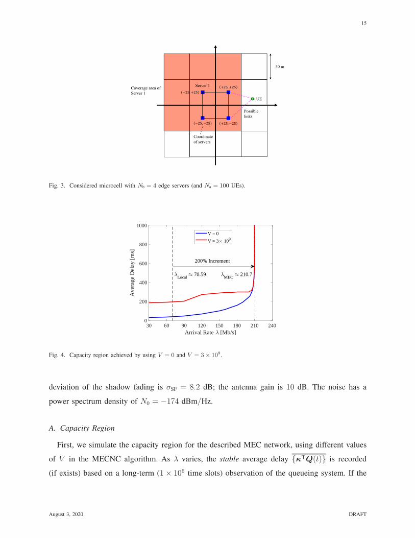
Fig. 3. Considered microcell with Nb = 4 edge servers (and Na = 100 UEs).

30 60 90 120 150 180 210 240Arrival Rate [Mb/s]

0

200

400

600

800

1000

Ave

rage

Del

ay [

ms]

V = 0

V = 3 109

Local 70.59

MEC 210.7

200% Increment

Fig. 4. Capacity region achieved by using V = 0 and V = 3× 109.

deviation of the shadow fading is σSF = 8.2 dB; the antenna gain is 10 dB. The noise has a

power spectrum density of N0 = −174 dBm/Hz.

A. Capacity Region

First, we simulate the capacity region for the described MEC network, using different values

of V in the MECNC algorithm. As λ varies, the stable average delay {κTQ(t)} is recorded

(if exists) based on a long-term (1 × 106 time slots) observation of the queueing system. If the


16

0 1 2 3 4 5

V 1010

0

0.5

1

1.5

2

2.5D

elay

[s]

0

0.1

0.2

0.3

0.4

0.5

0.6

Cost

optimal cost = 0.0084

45% Reduction

delay = 218 ms

cost = 0.033

Fig. 5. Delay and cost performance under various V .

0 1 2 3 4 5V 1010

0

0.05

0.1

0.15

0.2

0.25

0.3

Cos

t

Processing CostTransmission Cost (wired)Transmission Cost (wireless)

Fig. 6. Cost breakdown for processing and transmission part.

average delay is constantly growing even at the end of the time window, the average delay is

defined as ∞, which implies that the network is not stable under the given arrival rate.

As depicted in Fig. 4, the average delay rises as the arrival rate λ increases, which blows

up when approaching λMEC ≈ 210 Mb/s. This critical point can be interpreted as the boundary

of the capacity region of the MEC network. On the other hand, if all the computations are

constrained to be executed at the UEs, the capacity region is reduced to λLocal ≈ 70 Mb/s.8

That is, a gain of 200% is achieved with the aid of edge servers. Last but not least, note that

different V values lead to identical critical points, although they result in different average delay

performance, which validates the throughput-optimality of the MECNC algorithm.

B. Cost-Delay Tradeoff

Next, we study the delay and cost performance of the MEC network, when tuning the parameter

V . The arrival rate is set as λ = 100 Mb/s (i.e., 100 packets per slot).

The results are shown in Fig. 5. Evidently, the average delay9 grows almost linearly with

V , while the cost reduces as V grows (with a vanishing rate at the end), which support the

[O(V ), O(1/V )] tradeoff between the delay and cost bound. In addition, we observe two regions

of significant cost reduction, i.e., V ∈ [0, 3 × 109] and [2 × 1010, 3 × 1010]. The first reduction

8At the boundary of the capacity region, the computing capability constraint is active, i.e. λLocal

∑2φ=1

∑2m=1 Ξ

(m)φ w

(m)φ =

CKi(i ∈ Va).

9The result here is obtained by counting the age of the packets.


17

TABLE II

OFFLOADING RATIO UNDER DIFFERENT VALUES OF V

Service 1 Service 2

Function 1 Function 2 Function 1 Function 2

V = 0 20.0% 19.3% 56.7% 63.9%

V = 1× 109 59.8% 56.3% 75.1% 91.4%

V = 3× 109 98.8% 98.1% 99.7% 100%

is due to the task offloading to the edge cloud; while the second one results from cutting off

the connections between the edge servers, which lessens the transmission cost within the edge

cloud, while dramatically increasing the queueing delay (since we are not able to balance the

load between the edge servers in favor of delay performance). A more detailed cost breakdown

for the cost of each part is shown in Fig. 6.

Based on the tradeoff relationship, we can tune the value of V to optimize the performance

of practical MEC networks. For example, the value V ⋆ = 3× 109 leads to an average delay of

218 ms, which is acceptable for real-time applications; while a cost of 0.33, which reduces the

gap to the optimal cost 0.084 by 45% (compared with 0.53 when V = 0).

Finally, we observe the offloading ratios for different computation tasks and various V values in

Table II. As we expect, a growing value of V puts more attention to the induced cost, motivating

the UEs to offload the tasks to the cloud. In addition, we find that for all listed values of V ,

the functions of Service 2 tend to have a higher offloading ratio. An intuitive explanation is

that Service 2 is more compute-intensive, while resulting in lower communication overhead than

Service 1, and thus more preferable for offloading.

VI. CONCLUSIVE REMARKS

In this paper, we leveraged recent advances in the use of Lyapunov optimization theory to study

the stability of computing networks, in order to address key open problems in MEC network

control. We designed a distributed algorithm, MECNC, that makes joint decisions about task

offloading, packet scheduling, and computation/communication resource allocation. Numerical

experiments were carried out on the capacity region, cost-delay tradeoff, and task assignment


18

performance of the proposed solution, proving to be a promising paradigm to manage next

generation MEC networks.

APPENDIX A

PROOF OF THEOREM 1

Necessity: We start with the discrete case, where we collect the possible CSIs that can be

observed by node i in Gi, and the transmission actions that node i can take in Zi, and we

assume that the cardinalities of the sets are G and Z, respectively. We clarify that 1) each

element in both sets is a vector composed of all the information of node i’s outgoing links,

which will be represented by its index in the set, i.e., 1 ≤ g ≤ G and 1 ≤ z ≤ Z; 2) given

the CSI and the transmission vector, the data rate of all the outgoing links are fixed, denoted

by Rij(g, z). The following discussions are straightforward to extend to the continuous scenario,

where we push G→ ∞ and Z → ∞ assuming uniform discretization.

Suppose there exists some control algorithm to stabilize the queueing system. We define the

following quantities within the first t time slots:

• X(u,φ,m)ip,k (t): the number of (u, φ,m)-packets that are processed at node i when the allocation

choice is k ∈ Ki, and later on successfully delivered to the destination;

• X(u,φ,m)pi,k (t): the number of (u, φ,m)-packets that are received by node i from its local

processor when the allocation choice is k ∈ Ki, and later on successfully delivered to the

destination;

• X(u,φ,m)ij,k (t): the number of (u, φ,m)-packets that are transmitted through wired link (i, j)

when the allocation choice is k ∈ Lij , and later on successfully delivered to the destination.

• X(u,φ,m)ij,(g,z) (t): the number of (u, φ,m)-packets that are transmitted through wireless link (i, j)

when the observed CSI is g ∈ Gi and the adopted transmission vector is z ∈ Zi, and later

on successfully delivered to the destination.

• A(u,φ,m)i (t): the number of exogenous (u, φ,m)-packets that arrives at node i, and later on

successfully delivered to the destination.

Define the consumed computing resource

Si,k(t) =∑

(u,φ,m)

r(m)φ X

(u,φ,m)ip,k (t) (∀ k ∈ Ki), Si(t) =

∑

k∈Ki

Si,k(t) (37)


19

for wired transmission (i, j) ∈ Eb,

Xij,k(t) =∑

(u,φ,m)

X(u,φ,m)ij,k (t) (∀ k ∈ Kij), X

(u,φ,m)ij (t) =

∑

k∈Kij

X(u,φ,m)ij,k (t) (38)

and for wireless transmission (i, j) ∈ Ea,

Xij,(g,z)(t) =∑

(u,φ,m)

X(u,φ,m)ij,(g,z) (t) (∀ g ∈ Gi, z ∈ Zi), X

(u,φ,m)ij (t) =

∑

(g,z)∈Gi×Zi

X(u,φ,m)ij,(g,z) (t) (39)

In addition, we define N(i)k (t) as the number of time slots when node i assigns k ∈ Ki processing

resource; similarly, N(ij)k (t) can be defined for wired transmission with k ∈ Kij . For wireless

transmission, we define N(i)(g,z)(t) the number of time slots that the observed CSIs is g ∈ Gi, and

the transmission vector z ∈ Gi; and define N(i)g (t) =

∑

z∈ZiN

(i)(g,z)(t).

The following relationship then follows

∑

j∈δ−i

X(u,φ,m)ji (t) +X

(u,φ,m)pi (t) + A

(u,φ,m)i (t) =

∑

j∈δ+i

X(u,φ,m)ij (t) +X

(u,φ,m)ip (t) (40a)

X(u,φ,m+1)pi (t) = ξ

(m)φ X

(u,φ,m)ip (t) (40b)

r(m)φ X

(u,φ,m)ip (t) ≤

∑

k∈Ki

N(i)k (t)

(

r(m)φ X

(u,φ,m)ip,k (t)

Si,k(t)

)

Ci,k (40c)

X(u,φ,m)ij (t) ≤

∑

k∈Kij

N(ij)k (t)

(

X(u,φ,m)ij,k (t)

Xij,k(t)

)

Cij,k (40d)

X(u,φ,m)ij (t) ≤ τ

∑

(g,z)∈Gi×Zi

(

X(u,φ,m)ij,(g,z) (t)

Xij,(g,z)(t)

)(

N(i)(g,z)(t)

N(i)g (t)

)

N (i)g (t)Rij(z, g) (40e)

where (40d) is for (i, j) ∈ Eb and (40e) is for (i, j) ∈ Ea. The last three inequalities are interpreted

as follows, which are derived from the resource constraints. For the processing resource at node

i, consider the subset of time slots where k ∈ Ki processing resource is assigned, and we obtain

Si,k(t) ≤ N(i)k (t)Cij,k (∀ k ∈ Ki). (41)

Multiply by(

r(m)φ X

(u,φ,m)ip (t)

)

/Si,k(t), then sum over k ∈ Ki, and it leads to (40c). Similar

technique can be used to derive (40d) and (40e).


20

Divide (40) by t, and push t→ ∞. For simplicity, assume that all the limits exist, and define

limt→∞

X(u,φ,m)ip (t)

t= f

(u,φ,m)ip , lim

t→∞

X(u,φ,m)ij (t)

t= f

(u,φ,m)ij , lim

t→∞

A(u,φ,m)i (t)

t= λ

(u,φ,m)i

limt→∞

r(m)φ X

(u,φ,m)ip,k (t)

Si,k(t)= ℓ

(i)(u,φ,m)|k, lim

t→∞

X(u,φ,m)ij,k (t)

Xij,k(t)= ℓ

(ij)(u,φ,m)|k, lim

t→∞

X(u,φ,m)ij,(g,z) (t)

Xij,(g,z)(t)= ℓ

(ij)(u,φ,m)|(g,z)

limt→∞

N(i)k (t)

t= α

(i)k , lim

t→∞

N(ij)k (t)

t= α

(ij)k , lim

t→∞

N(i)(g,z)(t)

N(i)g (t)

= ϕ(i)z|g, lim

t→∞

N(i)g (t)

t= P

(i)g (42)

where P(i)g is the probability that the observed CSIs by node i is g. Substitute the above definitions

into the previous relationships, and the proof is concluded.

Furthermore, let G→ ∞ and Z → ∞, and we assume ϕ(i)z|g → ψ

(i)p|g, and P

(i)g converges to the

true CSIs distribution. In this case, (40e) becomes

f(u,φ,m)ij (t) ≤ τ

∑

(g,z)∈Gi×Zi

ℓ(ij)(u,φ,m)|(g,z)ϕ

(i)z|gP

(i)g Rij(z, g)

→ τ

∫

z∈Zi

ℓ(ij)(u,φ,m)|(g,z)ψ

(i)z|gp

(i)g Rij(z, g)dzdg

= τ

∫

Pi

Egi

{

ℓ(ij)(u,φ,m)|(gi,pi)

ψ(i)pi|gi

Rij(pi, gi)}

dpi

(43)

where we recall that each index z (or g) corresponds to an action (or CSI) vector.

Finally, assume that the control algorithm considered above leads to the optimal cost h⋆(λ).

By definition, we can obtain

h⋆(λ) =1

T

T∑

t=1

h(D(t)) =1

T

∑

D∈D

ND(T )h(D) (44)

where D denotes the action space, and ND(T ) is the number of time slots that action D is

selected within the observed interval. Further note that the constructed randomized policy ∗ (as

is introduced in Section III) satisfies that (by law of large number)

limT→∞

N∗D(T )

T= lim

T→∞

ND(T )

T(45)

where N∗D(T ) is the number of time slots that policy ∗ chooses the action D. It follows that

limt→∞

1

T

T∑

t=1

h(D∗(t)) = limt→∞

1

T

∑

D∈D

N∗D(T )h(D) = lim

t→∞

1

T

∑

D∈D

ND(T )h(D) = h⋆(λ) (46)

Therefore, the policy ∗ also achieves the optimal cost.


21

Sufficiency: We consider the stationary randomized policy constructed using the probability

value α, ψ and ℓ, as is explained in Section III. The resulting flow variables µ(u,φ,m)ij (t) is i.i.d.

over time slots, and by (13c) to (13e) we have

E

{

µ(u,φ,m)i,pr (t)

}

= E

{

E

{

µ(u,φ,m)i,pr (t)

∣

∣

∣ki

}}

= E

{

ℓ(i)(u,φ,m)|ki

(

Ci,ki

r(m)φ

)}

=1

r(m)φ

∑

ki∈Ki

α(i)kiℓ(i)(u,φ,m)|ki

Ci,ki = f(u,φ,m)i,pr (47)

E

{

µ(u,φ,m)ij (t)

}

= E

{

E

{

µ(u,φ,m)ij (t)

∣

∣

∣kij

}}

= E

{

ℓ(ij)(u,φ,m)|kij

Cij,kij

}

=∑

kij∈Kij

α(ij)k ℓ

(ij)(u,φ,m)|kij

Cij,kij = f(u,φ,m)ij (48)

E

{

µ(u,φ,m)ij (t)

}

= E

{

E

{

µ(u,φ,m)ij (t)

∣

∣

∣gi

}}

= E

{

τ

∫

Pi


Rij(pi, gi)ψ(i)pi|gi

dpi

}

= τ

∫

Pi

Egi

{


Rij(pi, gi)ψ(i)pi|gi

}

dpi = f(u,φ,m)ij (49)

Besides, it follows (13b) that

E

{

µ(u,φ,m)pr,i (t)

}

= E

{

ξ(φ,m)µ(u,φ,m−1)i,pr (t)

}

= ξ(φ,m)f(u,φ,m−1)i,pr = f

(u,φ,m)pr,i (50)

Substitute the above results into (13a), we obtain

E

{

∑

j

µ(u,φ,m)ji (t) + µ

(u,φ,m)pr,i (t) + a

(u,φ,m)i (t)

}

≤ E

{

∑

j

µ(u,φ,m)ij (t) + µ

(u,φ,m)i,pr (t)

}

(51)

Recall the queueing dynamics of Q(u,φ,m)i (t), where left-side and right-side in above equation

denote the incoming and outgoing packets of the queue, respectively. It indicates that Q(u,φ,m)i (t)

is mean rate stable [12].

APPENDIX B

PROOF FOR THEOREM 2

Note that the LDP expression satisfies

∆(t) + V h1(D(t)) ≤ B0 + V h1(D(t))

−∑

i,(d,φ,m)

[

∑

j∈δ+i


(u,φ,m)i,pr (t)−

∑

j∈δ−i

µ(u,φ,m)ji (t)− µ

(u,φ,m)pr,i (t)− a

(u,φ,m)i (t)

]

Q(u,φ,m)i (t)

≤ B0 + V h1(D(t))

−∑

i,(d,φ,m)

[

∑

j∈δ+i


(u,φ,m)i,pr (t)−

∑

j∈δ−i



(u,φ,m)i (t)

]

Q(u,φ,m)i (t)

(52)


22

where D (which includes the decisions on flow assignment µ) is the decision made by the

stationary randomized policy that achieves minimum cost for arrival rate λ+ ǫ1, which can be

constructed according to Appendix A (the existence of ǫ is guaranteed since λ is in the interior

of the capacity region).

Note the following facts about the decision D(t): 1) it is a stationary randomized policy, thus

the decisions, specially µ(t), are independent with Q(t), 2) this policy is cost optimal for arrival

rate λ+ ǫ1, i.e., E{

h(D(t))}

= h⋆(λ+ ǫ1), 3) the network is stabilized using this randomized

algorithm under λ+ ǫ1, thus

E

∑

j∈δ+i


(u,φ,m)i,pr (t)−

∑

j∈δ−i



(u,φ,m)i (t)

≥ 0 (53)

where a(u,φ,m)i (t) is an (imaginary) arriving process with mean λ

(u,φ,m)i + ǫ, which indicates

E

∑

j∈δ+i


(u,φ,m)i,pr (t)−

∑

j∈δ−i


(u,φ,m)pr,i (t)

− λ(u,φ,m)i ≥ ǫ. (54)

Then we take expectation of (52), and use the above facts

E {∆(t) + V h1(D(t))} ≤ B0 + V h⋆1(λ+ ǫ1)− ǫ∑

i,(d,φ,m)

E

{

Q(u,φ,m)i (t)

}

(55)

It immediately gives (by telescoping sum, see [12] for details)

limT→∞

1

T

T−1∑

t=0

E {h1(D(t))} ≤ h⋆1(λ+ ǫ1) +B0

V(56)

limT→∞

1

T

T−1∑

t=0

∑

i,(d,φ,m)

E

{

Q(u,φ,m)i (t)

}

≤B0

ǫ+

[

h⋆1(λ+ ǫ1)− h⋆1(λ)

ǫ

]

V. (57)

Recall the definition of Q(t) in (20), as well as its relationship to the average (queueing) delay

(9), and (57) is equivalent to

h2 =∑

i,(d,φ,m)

{

Q(u,φ,m)i (t)

}

≤B0

ǫ+

[

h⋆1(λ+ ǫ1)− h⋆1(λ)

ǫ

]

V. (58)

On the other hand, note that (56) holds for every ǫ > 0, and therefore it holds for a sequence

{ǫn}n>0 ↓ 0, which implies

h1 = {h1(D(t))} ≤ h⋆1(λ) +B0

V. (59)


23

REFERENCES

[1] H. T. Dinh, C. Lee, D. Niyato, and P. Wang, “A survey of mobile cloud computing: architecture, applications, and

approaches,” Wirel. Commun. Mob. Comput., vol. 13, no. 18, pp. 1587–1611, Dec. 2013.

[2] P. Mach and Z. Becvar, “Mobile edge computing: A survey on architecture and computation offloading,” IEEE

Communications Surveys & Tutorials, vol. 19, no. 3, pp. 1628–1656, Mar. 2017.

[3] M. Chen and Y. Hao, “Task offloading for mobile edge computing in software defined ultra-dense network,” IEEE J. Sel.

Areas Commun., vol. 36, no. 3, pp. 587–597, Mar. 2018.

[4] X. Lyu, H. Tian, W. Ni, Y. Zhang, P. Zhang, and R. P. Liu, “Energy-efficient admission of delay-sensitive tasks for mobile

edge computing,” IEEE Trans. Commun., vol. 66, no. 6, pp. 2603–2616, Jun. 2018.

[5] T. X. Tran and D. Pompili, “Joint task offloading and resource allocation for multi-server mobile-edge computing networks,”

IEEE Trans. Veh. Technol., vol. 68, no. 1, pp. 856–868, Jan. 2019.

[6] M. Barcelo, J. Llorca, A. M. Tulino, and N. Raman, “The cloud service distribution problem in distributed cloud networks,”

in Proc. IEEE Int. Conf. Commun., London, UK, May 2015, pp. 344–350.

[7] M. F. Bari, S. R. Chowdhury, R. Ahmed, and R. Boutaba, “On orchestrating virtual network functions in NFV,” in 11th

Int. Conf. on Network and Service Management (CNSM), Barcelona, Spain, Nov. 2015, pp. 50–56.

[8] D. Bhamare, R. Jain, M. Samaka, and A. Erbad, “A survey on service function chaining,” Journal of Network and Computer

Applications, vol. 75, no. 1, pp. 138–155, Nov. 2016.

[9] H. Feng, J. Llorca, A. M. Tulino, and A. F. Molisch, “Optimal dynamic cloud network control,” IEEE/ACM Trans. Netw.,

vol. 26, no. 5, pp. 2118–2131, Oct. 2018.

[10] ——, “Optimal control of wireless computing networks,” IEEE Trans. Wireless Commun., vol. 17, no. 12, pp. 8283–8298,

Dec. 2018.

[11] A. Adhikary, J. Nam, J.-Y. Ahn, and G. Caire, “Joint spatial division and multiplexing – The large-scale array regime,”

IEEE Trans. Inf. Theory, vol. 59, no. 10, pp. 6441–6463, Oct. 2013.

[12] M. J. Neely, Stochastic network optimization with application to communication and queueing systems. San Rafael, CA,

USA: Morgan & Claypool, 2010.


Mobile Edge Computing Network Control: Tradeoff Between ...

Documents

Transcript of Mobile Edge Computing Network Control: Tradeoff Between ...