Mobile Communications: Technology and QoS · Mobile Communications: Technology and QoS Course...
37
Mobile Communications: Technology and QoS Course Overview Marc Kuhn, Yahia Hassan [email protected] / [email protected] Institut für Kommunikationstechnik (IKT) Wireless Communications Group ETH Zürich 1
Transcript of Mobile Communications: Technology and QoS · Mobile Communications: Technology and QoS Course...

Mobile Communications: Technology and QoS
Course Overview !
Marc Kuhn, Yahia Hassan [email protected] / [email protected] Institut für Kommunikationstechnik (IKT)
Wireless Communications Group ETH Zürich
1

MCTQ: Overview of the Course
(a few selected slides per chapter) !
Dr.- Ing. Marc Kuhn [email protected] !
Institut für Kommunikationstechnik (IKT), !Wireless Communications Group !
ETH Zürich!!
2

Contents
Introduction!
Wireless Channel !
Mobile Communication!
Wireless Networks!
Quality of Service – QoS !
Future Technologies
3

Contents
Introduction!
Wireless Channel !
Mobile Communication!
Wireless Networks!
Quality of Service – QoS !
Future Technologies
4

Wireless Channel
Propagation Channel !Maxwell equations, system functions of wireless channels!
Multipath Propagation !
Path loss!
Doppler Effect!
Channel Characterization, Channel Models!Fading, delay spread, Doppler spread, coherence time and bandwidth, channel models !
Antennas
5

Wireless Channel: Observations
Channel strength (attenuation) and thus SNR at Rx varies !
depending on the location (space-selective fading)!
over time (time-selective fading)!
over frequency (frequency-selective fading)!
Bandwidth limited!
Shared medium!interference
6

Basic Propagation Mechanisms
Reflection!Propagating electromagnetic wave impinges on object with very large dimension compared to wavelength !
Reflection e.g. from buildings and walls (or from surface of earth)!
Diffraction!Radio path between Tx and Rx obstructed by a surface that has sharp irregularities!
Scattering!Between Tx and Rx: objects with dimensions small compared to the wavelength
7

Multipath Propagation: Location-Dependent Fading
8
at a given frequency f1 r1
r2
r4
rTX
Position BPosition Ar2
rTX
r3
r1
|rTX| [dB]
location x

Wireless Channel
Large-scale fading!Received power decreases with distance r!
e.g. free space: 1/r² !
can even be faster due to shadowing and scattering effects!
!
Small-scale fading!Variation of signal strength over distances of the order of the carrier wavelength, due to constructive and destructive interference of multi-paths!
Doppler spread, coherence time (e.g. due to velocity of mobile)!
Delay spread, coherence bandwidth (lengths of shortest and longest path)
9
➡ Relevant to design of communication systems
➡ Relevant to cell-site planning

Narrowband System
[Molisch, “Wireless Communications“]
10
Wideband and Directional Channel Characterization 105
The above considerations also lead us to a mathematical formulation for narrowband and wide-band from a time domain point of view: a system is narrowband if the inverse of the systembandwidth 1/W is much larger than the maximum excess delay τmax. In that case, all echoes fallinto a single delay bin, and the amplitude of this delay bin is α(t). A system is wideband in allother cases. In a wideband system, the shape and duration of the arriving signal is different fromthe shape of the transmitted signal; in a narrowband system, they stay the same.
If the impulse response has a finite extent in the delay domain, it follows from the theoryof Fourier transforms (FTs) that the transfer function F{h(τ )} = H(f ) is frequency dependent.Delay dispersion is thus equivalent to frequency selectivity . A frequency-selective channel cannotbe described by a simple attenuation coefficient, but rather the details of the transfer function mustbe modeled. Note that any real channel is frequency selective if analyzed over a large enoughbandwidth; in practice, the question is whether this is true over the bandwidth of the consideredsystem. This is equivalent to comparing the maximum excess delay of the channel impulse responsewith the inverse system bandwidth. Figure 6.4 sketches these relationships, demonstrating thevariations of wideband systems in the delay and frequency domain.
We stress that the definition of a wideband wireless system is fundamentally different fromthe definition of “wideband” in the usage of Radio Frequency (RF) engineers. The RF definition
Wideband system
Narrowband system
|Hc(f )| |Hs(f )| |H(f )|
1/∆tmax f f f
X =
=
|hc(t )| |hs(t )| |h(t )|
|Hc(f )| |Hs(f )| |H(f )|
|hc(t )| |hs(t )| |h(t )|
∆tmax t t t
X =
=
f f f
t t t
1/∆tmax
∆tmax
Figure 6.4 Narrowband and wideband systems. HC(f ), channel transfer function; hC(τ ), channel impulseresponse.Reproduced with permission from Molisch [2000] © Prentice Hall.

Wideband (or Broadband) System
[Molisch, “Wireless Communications“]
11
Wideband and Directional Channel Characterization 105
The above considerations also lead us to a mathematical formulation for narrowband and wide-band from a time domain point of view: a system is narrowband if the inverse of the systembandwidth 1/W is much larger than the maximum excess delay τmax. In that case, all echoes fallinto a single delay bin, and the amplitude of this delay bin is α(t). A system is wideband in allother cases. In a wideband system, the shape and duration of the arriving signal is different fromthe shape of the transmitted signal; in a narrowband system, they stay the same.
If the impulse response has a finite extent in the delay domain, it follows from the theoryof Fourier transforms (FTs) that the transfer function F{h(τ )} = H(f ) is frequency dependent.Delay dispersion is thus equivalent to frequency selectivity . A frequency-selective channel cannotbe described by a simple attenuation coefficient, but rather the details of the transfer function mustbe modeled. Note that any real channel is frequency selective if analyzed over a large enoughbandwidth; in practice, the question is whether this is true over the bandwidth of the consideredsystem. This is equivalent to comparing the maximum excess delay of the channel impulse responsewith the inverse system bandwidth. Figure 6.4 sketches these relationships, demonstrating thevariations of wideband systems in the delay and frequency domain.
We stress that the definition of a wideband wireless system is fundamentally different fromthe definition of “wideband” in the usage of Radio Frequency (RF) engineers. The RF definition
Wideband system
Narrowband system
|Hc(f )| |Hs(f )| |H(f )|
1/∆tmax f f f
X =
=
|hc(t )| |hs(t )| |h(t )|
|Hc(f )| |Hs(f )| |H(f )|
|hc(t )| |hs(t )| |h(t )|
∆tmax t t t
X =
=
f f f
t t t
1/∆tmax
∆tmax
Figure 6.4 Narrowband and wideband systems. HC(f ), channel transfer function; hC(τ ), channel impulseresponse.Reproduced with permission from Molisch [2000] © Prentice Hall.
Quasi-Static CIR
Quasi-static, h(t, τ) varies only slowly over time: !Variable t parameterizes the impulse response: which (out of a large ensemble) impulse response h(τ) is currently valid
12From [“Wireless Communications: Principles & Practice” T. Rappaport]

Multipath Propagation, Narrowband Fading
13
Multipath propagation:!constructive and destructive interference!
random fluctuations of receive power – (small-scale) Fading!
strong influence on quality of the transmission
mea
n

Contents
Introduction!
Wireless Channel !
Mobile Communication!
Wireless Networks!
Quality of Service – QoS !
Future Technologies
14
Mobile Communication
PHY Layer !OFDM !
MIMO !
Receiver structures !
MAC Layer !MAC: IEEE 802.11, .11e
15

OFDM
Continuous-time vs. discrete-time model !
16
Orthogonal Frequency Division Multiplexing (OFDM) 419
(a)
(b)
c0, i
c1, i
cN 1, i
cN 1, i
c0, i
c1, i
cN 1, i
Transmitter
Datasource
S/Pconversion
Datasource
S/Pconversion
c0, i
c1, i
Channel Receiver
e j2π(W/N)t
e j2π(N 1) (W/N)te j2π(N 1) (W/N)t
cN 1, i
s(t ) Hs(t )H
s(t ) Hs(t )H
e j0
c1, i
c0, i
P/Sconversion
P/Sconversion
Datasink
Datasink
e j2π(W/N)t
e j0
IFFT P/S S/P FFT
Figure 19.2 Transceiver structures for orthogonal frequency division multiplexing in purely analog technology(a), and using inverse fast Fourier transformation (b).
An alternative implementation is digital . It first divides the transmit data into blocks of Nsymbols. Each block of data is subjected to an Inverse Fast Fourier Transformation (IFFT), andthen transmitted (see Figure 19.2b). This approach is much easier to implement with integratedcircuits. In the following, we will show that the two approaches are equivalent.
Let us first consider the analog interpretation. Let the complex transmit symbol at time instanti on the nth carrier be cn,i . The transmit signal is then:
s(t) =∞!
i=−∞si(t) =
∞!
i=−∞
N−1!
n=0
cn,ign(t − iTS) (19.2)
where the basis pulse gn(t) is a normalized, frequency-shifted rectangular pulse:
gn(t) ="
1√TS
exp#j2πn t
TS
$for 0 < t < TS
0 otherwise(19.3)
Let us now – without restriction of generality – consider the signal only for i = 0, and sample itat instances tk = kTs/N :
sk = s(tk) = 1√TS
N−1!
n=0
cn,0 exp%
j2πnk
N
&(19.4)
Now, this is nothing but the inverse Discrete Fourier Transform (DFT) of the transmit symbols.Therefore, the transmitter can be realized by performing an Inverse Discrete Fourier Transform(IDFT) on the block of transmit symbols (the blocksize must equal the number of subcarriers).In almost all practical cases, the number of samples N is chosen to be a power of 2, and theIDFT is realized as an IFFT. In the following, we will only speak of IFFTs and Fast FourierTransforms (FFTs).
[A. Molisch, “Wireless Communications]

OFDMA
17
User 1 2 3 OFDM sub-carriers
Distributed OFDMA mode
Localized OFDMA mode

Diversity Techniques
18
Marc Kuhn
Tx Diversity: Alamouti Code (ST-Code)
! Vectors: elements in spatial domain
! Matrix S: 2 vectors in 2 time-slots
! Orthogonalize decision variables ! Two-fold diversity ! ! One symbol per time slot (more
efficient!) 22
s1 =s1
−s2*
⎛
⎝⎜⎜
⎞
⎠⎟⎟
s2 =s 2
s1*
⎛
⎝⎜⎜
⎞
⎠⎟⎟
S = s1s2⎡⎣ ⎤⎦ =s1
−s2*
s 2
s1*
⎛
⎝⎜⎜
⎞
⎠⎟⎟
r1 (1) = h1,1s1 − h1,2 s2* + w1 (1)
r1 (2) = h1,2 s1* + h1,1s2 + w1 (2) → r1
*(2) = h1,2* s1 + h1,1
* s2* + w1
*(2)
d(1) = h1,1* r1 (1) + h1,2r1
*(2) = h1,12s1 + h1,2
2s1 + n1
d(2) = −h1,2* r1 (1) + h1,1r1
*(2) = h1,12s2* + h1,2
2s2* +m1
Diversity, MIMO
Assume channel const. for 2 time slots:
2s
1,1h
1,2h
1s1r

MIMO
19
Marc Kuhn 33
TX RX
Diversity, MIMO
Telatar, Foschini:
MT: number of TX antennas, MR: number of RX antennas.
Multiple Input Multiple Output – MIMO
C = E log2 det I MR
+ES
MT N0
HHH⎛
⎝⎜⎞
⎠⎟⎡
⎣⎢⎢
⎤
⎦⎥⎥
⎧⎨⎪
⎩⎪
⎫⎬⎪
⎭⎪

20
Marc Kuhn
Capacity of MIMO Channels: Perfect CSIT
41
Diversity, MIMO
γ i = E si
2( ) , for i = 1, 2, ..., N
γ ii=1
N
∑ = MT
yi =
ES
MT
λi si + ni
! With perfect CSIT: - Tx combining to orthogonalize MIMO channel (multiply with unitary matrix V)
- Tx power per Eigenvalue has to be optimized (Water-filling algorithm) => choose optimal γi (energy allocated to sub-channel i) to maximize capacity
Tx signal : s = Vs where H = USV H
! λi +!si! yi!
wi!
CpCSIT = max
γ i1
N∑ =MT
log2 1+ES
MT N0
λi HHH{ } ⋅γ i
⎛
⎝⎜⎞
⎠⎟i=1
N
∑⎡
⎣⎢⎢
⎤
⎦⎥⎥

Multi-User MIMO
Uplink: Multiple Access Channel (MIMO-MAC) !
!
!
!
Downlink: Broadcast Channel (MIMO-BC)
21
WLAN IEEE 802.11
22
|!|!MCTQ: Wireless Networks, 802.11
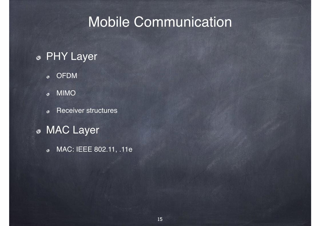
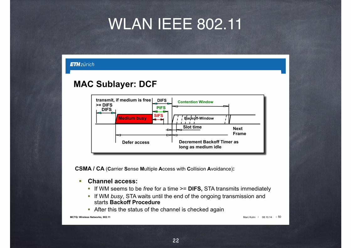
MAC Sublayer: DCF
! Channel access: ! If WM seems to be free for a time >= DIFS, STA transmits immediately ! If WM busy, STA waits until the end of the ongoing transmission and
starts Backoff Procedure ! After this the status of the channel is checked again
DIFS Contention Window
Slot time
Defer access
Backoff-Window
Next Frame
Decrement Backoff Timer as long as medium idle
SIFS PIFS DIFS
Medium busy
transmit, if medium is free >= DIFS
CSMA / CA (Carrier Sense Multiple Access with Collision Avoidance):
Wireless Networks, 802.11
Marc Kuhn 08.10.14 50

Contents
Introduction!
Wireless Channel !
Mobile Communication!
Wireless Networks!
Quality of Service – QoS !
Future Technologies
23

Wireless Networks
Current (and future) wireless networks:!How do they work?!
For which services are they used?!
Cellular Networks!GSM!
UMTS!
LTE, LTE-Advanced !
WLAN IEEE 802.11n
24

Cellular Networks
25
Mobile Communication
! Omnipresent ! 9.9 Mio. SIM cards in CH
(2012)
! 99.9 % of Swiss population covered
! Exponential increase in data traffic
! Different standards (GSM, UMTS, LTE, ... ) (2G, 3G, 4G)
11
Cellular Networks

Cellular Networks
26
Cellular Wireless: max. Downlink Rates
0.0096
0.1152 0.1712 0.4736 0.384
14.4
84.4 150
1000
0.001
0.01
0.1
1
10
100
1000
GSM CSD
HSCSD
GPRS
EDGE
UMTS
HSDPA
HSPA+ LT
E
LTE-A
dvan
ced
Pea
k da
ta r
ate
[Mbi
t/s]
! Techniques to achieve this almost exponential growth in peak rate
! Closer look on LTE and LTE-Advanced
Cellular Networks 12

Cellular Networks
27
Structure of Cellular Networks
x Position [m]
y Po
sitio
n [m
]
Mean Rate Rmean(SINR), DL, with BS interference
−1500 −1000 −500 0 500 1000 1500
−1500
−1000
−500
0
500
1000
1500 1e+07
2e+08
4e+08
6e+08
8e+08 1e+09 1.2e+091.4e+091.6e+091.8e+092e+09
200 Mbit/s
10 Mbit/s
2 Gbit/s
16
Cellular Networks

Coordinated Multi Point - CoMP
28

Contents
Introduction!
Wireless Channel !
Mobile Communication!
Wireless Networks!
Quality of Service – QoS !
Future Technologies
29

Quality of Service - QoS
What does QoS mean?!How is QoS support implemented in wireless networks?!
Which problems do occur? !
Theoretical analysis of QoS at PHY and MAC of wireless systems!
How can we measure QoS? !End-to-End QoS Measurements!
Statistical evaluation of QoS measurements!
Benchmarking (drive tests, methods)
30

PHY QoS KPIs
31
0 5 10 15 2010−5
10−4
10−3
10−2
10−1
100
P out
S / N [dB]
MIMO: Outage Probability for Outage Rate 6
(3x3) MIMO
(2x2) MIMO
(2x3) MIMO
(3x2) MIMO
0 2 4 6 8 10 120
0.1
0.2
0.3
0.4
0.5
0.6
0.7
0.8
0.9
1
Capacity [bit/channel use]
Cum
ulat
ive D
istrib
utio
n Fu
nctio
n
SISO: CDF of channel capacity ; Rayleigh fading
SNR = [0, 5, 10, 15, 20] dB
Outage Rate: 2 bit/ channel use!

MAC QoS KPIs
Example: IEEE 802.11 MAC
32

Quality of Service - QoS
What does QoS mean?!How is QoS support implemented in wireless networks?!
Which problems do occur? !
Theoretical analysis of QoS at PHY and MAC of wireless systems!
How can we measure QoS? !End-to-End QoS Measurements!
Statistical evaluation of QoS measurements!
Benchmarking (drive tests, methods)
33
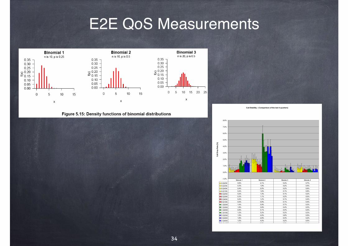
E2E QoS Measurements
34
Call Stability ( Comparison of the last 4 quarters)
-1,0%
0,0%
1,0%
2,0%
3,0%
4,0%
5,0%
6,0%
7,0%
8,0%
Cal
l Dro
p R
ate
[%]
A Q2/04 0,6% 2,1% 0,4% 0,7%
A Q3/04 0,3% 1,9% 0,2% 0,5%
A Q4/04 0,4% 2,0% 0,2% 0,6%
A Q1/05 0,4% 1,6% 0,1% 0,8%
B Q2/04 0,2% 1,3% 0,1% 0,2%
B Q3/04 0,3% 1,1% 0,2% 0,5%
B Q4/04 0,4% 1,2% 0,1% 0,4%
B Q1/05 0,5% 0,9% 0,1% 0,4%
C Q2/04 1,4% 5,9% 0,7% 0,5%
C Q3/04 1,8% 3,9% 0,4% 0,5%
C Q4/04 0,9% 3,1% 0,4% 0,4%
C Q1/05 1,2% 3,2% 0,2% 0,2%
D Q2/04 1,5% 4,0% 0,8% 0,5%
D Q3/04 1,8% 2,8% 0,4% 0,2%
D Q4/04 1,5% 4,0% 0,2% 0,5%
D Q1/05 1,4% 2,5% 0,0% 0,4%
Module 1 Module 2 Module 3 Module 4

35
Call Stability ( all Modules)
-0.5%
0.0%
0.5%
1.0%
1.5%
2.0%
2.5%
3.0%
3.5%
4.0%
4.5%
Cal
l Dro
p R
ate
[%]
A 0.4% 1.6% 0.1% 0.8%
B 0.5% 0.9% 0.1% 0.4%
C 1.2% 3.2% 0.2% 0.2%
D 1.4% 2.5% 0.0% 0.4%
Module 1 Module 2 Module 3 Module 4
Won Pairwise comparisons: Coverage Quality ()
-6
-5
-4
-3
-2
-1
0
1
2
3
4
5
Won
Pai
rwis
e co
mpa
rison
s: C
all S
etup
Suc
cess
Rat
e
A 0 2 -2 0 0
B 0 2 2 0 4
C 1 -2 2 0 1
D -1 -2 -2 0 -5
Module 1 Module 2 Module 3 Module 4 All Modules

Contents
Introduction!
Wireless Channel !
Mobile Communication!
Wireless Networks!
Quality of Service – QoS !
Future Technologies
36

Future Technologies
Base station or user cooperation!
Relaying !
Interference alignment !
...
37