MNC Related Doc
82
Accounting for the Growth of MNC-based T rade using a Structural Model of U.S. MNCs † Susan E. Feinberg Robert H. Smith School of Business University of Maryland 3423 Van Munching Hall College Park, MD 20742-1815 (301) 405-2251 [email protected] Michael P. Keane Department of Economics Yale University 37 Hillhouse Avenue Room 29 New Haven, CT 06520-8264 (203) 432-3548 [email protected] January, 2003 † The statistical analysis of the confidential firm-level data on U.S. multinational corporations reported in this study was conducted at the International Investment Division, Bureau of Economic Analysis, U.S. Department of Commerce, under arrangemen ts that maintained l egal confidentiality requirements. The views expressed are those o f the authors and do not necessarily reflect those of the Department of Commerce. Suggestions and assistance from William Zeile, Raymond Mataloni and Lorraine Eden are gratefully acknowledged. Comments by Keith Head, Kala Krishna, Jim Tybout, Sam Kortum, Bernie Yeung and other participants in the NBER Universities Research Conference on Firm Level Responses to Trade Policy are greatly appreciated. We have also received helpful comments from seminar participants at Yale, ASU and the U.S. International Trade Commission, especially Penny Goldberg and T.N. Srinivasan, along with Russ Hilberry, Jason Cummins and Richard Rogerso n.
-
Upload
owaiskhanm -
Category
Documents
-
view
219 -
download
0
Transcript of MNC Related Doc
7/29/2019 MNC Related Doc
http://slidepdf.com/reader/full/mnc-related-doc 1/82
Accounting for the Growth of MNC-based Trade
using a Structural Model of U.S. MNCs†
Susan E. FeinbergRobert H. Smith School of Business
University of Maryland
3423 Van Munching HallCollege Park, MD 20742-1815(301) 405-2251
Michael P. KeaneDepartment of Economics
Yale University37 Hillhouse Avenue Room 29 New Haven, CT 06520-8264
(203) [email protected]
January, 2003
† The statistical analysis of the confidential firm-level data on U.S. multinational corporations reported in this studywas conducted at the International Investment Division, Bureau of Economic Analysis, U.S. Department of Commerce, under arrangements that maintained legal confidentiality requirements. The views expressed are those of the authors and do not necessarily reflect those of the Department of Commerce. Suggestions and assistance fromWilliam Zeile, Raymond Mataloni and Lorraine Eden are gratefully acknowledged. Comments by Keith Head, KalaKrishna, Jim Tybout, Sam Kortum, Bernie Yeung and other participants in the NBER Universities ResearchConference on Firm Level Responses to Trade Policy are greatly appreciated. We have also received helpfulcomments from seminar participants at Yale, ASU and the U.S. International Trade Commission, especially PennyGoldberg and T.N. Srinivasan, along with Russ Hilberry, Jason Cummins and Richard Rogerson.

7/29/2019 MNC Related Doc
http://slidepdf.com/reader/full/mnc-related-doc 2/82
Abstract
U.S. foreign trade has grown much more rapidly than GDP in recent decades. But there isno consensus as to why. More than half of U.S. foreign trade consists of arms-length and intra-firm trade activity by multinational corporations (MNCs). Thus, in order to better understand the
growth of trade, it is important to understand the reasons for the rapid growth in MNC-basedtrade.This paper uses confidential BEA data on the activities of U.S. MNCs to shed light on
this issue. Specifically, we estimate a simple structural model of the production and tradedecisions of U.S. MNCs with affiliates in Canada, the largest trading partner of the U.S., usingdata from 1983-96. We then use the model as a framework to decompose the growth in intra-firm and arms-length trade flows into components due to tariff reductions, changes intechnology, changes in wages, and other factors.
We find that tariff reductions can account for a substantial part of the increase in arms-length MNC-based trade. But our model attributes most of the growth of intra-firm trade totechnical change, with tariff reductions playing only a secondary role. Simple descriptive
statistics provide face validity for this result, since arms-length trade grew much more rapidly inindustries with the largest tariff reductions, while intra-firm trade grew rapidly even in industrieswhere tariffs were negligible to begin with.
Our work makes a number of other contributions: Our descriptive analysis of the BEAfirm level data, which has rarely been made available for research, suggests that few MNCs fitinto the neat vertical vs. horizontal dichotomy of the theoretical literature. Also, we find thatMNC decisions to engage in intra-firm and arms-length trade are unrelated to tariff levels. Thegrowth in MNC-based trade due to tariff reductions has been almost entirely on the intensivemargin, among the subset of firms already engaged in such activities.
Finally, the estimation of our model requires the development of a number of neweconometric procedures. We present new recursive importance sampling algorithms that are thecontinuous and discrete/continuous analogues of the GHK method.

7/29/2019 MNC Related Doc
http://slidepdf.com/reader/full/mnc-related-doc 3/82
1
I. Introduction
In recent decades, trade has grown much more rapidly than GDP. Indeed, between 1982
and 1994, the growth of U.S. foreign trade (exports plus imports) averaged more than 5% per
year in real terms, while real GDP grew only 3% per year. Although the rapid growth of trade
has been widely documented, there is no consensus on its source (see Bergoeing and Kehoe
(2001) and Yi (2000) for recent discussions of this issue).
In order to understand the sources of growth of trade, it is important to understand the
behavior of multinational corporations (MNCs). According to Rugman (1988), over half of
world trade involves MNCs. Such MNC-based trade includes two components: arms-length
trade, which are shipments between a division of an MNC and unaffiliated buyers/suppliers in
other countries, and intra-firm trade, which are internal shipments between an MNC parent and
its foreign affiliates. Between 1982 and 1994, the total trade of U.S. based MNCs grew an
average of 4.5% per year. And the intra-firm component grew more rapidly than the arms-length
component.1 Indeed, between 1982 and 1994, intra-firm trade increased from 35.5% to 45% of
the total trade of US-based MNCs. What explains the rapid growth in MNC-based trade in
general, and the even faster growth of intra-firm trade between divisions of MNCs in particular?
In this paper, we analyze the sources of the growth in trade activity by U.S. MNCs with
affiliates in Canada, the largest trading partner of the U.S.. We estimate a structural model of the
MNCs’ production and trade decisions, using a confidential disaggregated panel data set from
the Bureau of Economic Analysis on more than 500 U.S. MNCs and their Canadian affiliates
from 1983-1996. We then use the model as a framework to decompose changes in intra-firm and
arms-length trade flows into components due to changes in tariffs, changes in technology,
changes in wages, and other factors (i.e., changes in prices, exchange rates, etc.).
There were significant bilateral tariff reductions between the U.S. and Canada during our
sample period, arising both from the GATT/WTO and the Canada-U.S. Free Trade Agreement
(FTA) in 1989, as is shown in Figure 1. This figure makes clear that tariff reductions were
gradual, and not concentrated in the immediate aftermath of the FTA. As we will see, there was
also substantial variation across industries in the extent of tariff reductions. Thus, the U.S.-
Canada context provides an excellent opportunity to examine the contribution of trade
liberalization to the observed increases in MNC based trade.2
1 For US MNCs, these trade flows grew an average of 3.4% and 6.3% per year, respectively. We do not include inthese statistics trade to and from U.S. affiliates of foreign MNCs. All our aggregate statistics on the growth of tradeare derived from figures presented in Zeile (1997).2 As Trefler (2001) points out, most trade liberalizations are accompanied by packages of economic reforms, makingthe pure effect of tariffs difficult to isolate. A notable example is NAFTA, which included removal of constraints on
7/29/2019 MNC Related Doc
http://slidepdf.com/reader/full/mnc-related-doc 4/82
2
One significant contribution of our work is simply to use the confidential firm level BEA
data to provide a description of the production and trade arrangements of U.S. MNCs and their
foreign affiliates. Many aspects of MNC organization that we observe in the data are rather
surprising from the perspective of the extant theories of the MNC. As a consequence, there is no
“off-the-shelf” model of MNC behavior that we can estimate structurally on the BEA data. The
main problem is that existing theories of the MNC cannot explain the multiplicity of MNC
production arrangements we see in the data.
Markusen and Maskus (1999a, b) provide an excellent discussion of the existing theories
of the MNC. As they note, these theories can be divided into those that generate vertical vs.
horizontal MNCs. Classic examples of these two types of models are Helpman (1984) and
Markusen (1984), respectively. Vertical MNCs fragment the production process across countries
to take advantage of factor price differentials, e.g., by locating unskilled-labor intensive parts of
the process in low wage countries. Horizontal MNCs basically replicate the entire production
process in multiple countries, thus avoiding tariff and transport costs.
The MNC forms we observe in the BEA data do not, for the most part, fall into the neat
vertical/horizontal taxonomy that exists in the theories. Models of horizontal MNCs rule out
substantial intra-firm flows of intermediates essentially by definition.3 But inspection of the
BEA firm level data on US. MNC parents and their Canadian affiliates suggests that vertical
specialization – the fragmentation of production processes into parts that are performed in
different countries - is indeed pervasive. We find that the value of intermediates shipped from
U.S. parents to their Canadian affiliates is, on average, more than one-third of affiliate total sales.
And the value of intermediates shipped by affiliates to parents is, on average, 39% of affiliate
total sales. Only about 12% of the firms in the BEA data are pure “horizontal” MNCs, in the
sense of having negligible intra-firm flows of intermediates.
But standard vertical MNC models do not describe the data either. The classic models of
Helpman (1984, 1985) and Helpman and Krugman (1985) do generate intra-firm trade in
intermediates, but it goes in only one direction. For instance, in Helpman and Krugman, MNCs
foreign direct investment (FDI) in Mexico. To a great extent, the U.S.-Canada FTA did not combine tariff reductionswith other major policy changes, making it, according to Trefler, an “unusually clean trade policy exercise.”3 Obviously, simple horizontal models also fail to generate arms-length sales of final goods (either by the parent tothe host country or by the affiliate back to the home country), since FDI is used to avoid such trade in these models.But Brander (1981) showed how horizontal models can be modified to generate bilateral arms length trade in similar goods by assuming the final goods produced by the parent and affiliate are differentiated. Recently, Baldwin andOttaviano (1998) have extended Brander’s model to also generate intra-industry FDI. We note that Rugman (1985)has quantified the importance of bilateral intra-industry trade and FDI at the aggregate industry/country level.

7/29/2019 MNC Related Doc
http://slidepdf.com/reader/full/mnc-related-doc 5/82
3
produce a differentiated product in three stages that require descending levels of capital intensity:
headquarters services, production of intermediates and production of final goods. Suppose the
factor prices are such that headquarters services and intermediate goods production are located in
the home country and final assembly is done by the foreign affiliate. This leads to a one-way
flow of intermediates from parent to affiliate.4 But a striking aspect of the BEA data is the
number of cases in which intra-firm flows actually go in both directions - 69% of observations.5
Furthermore, this prevalence of bilateral intra-firm flows of intermediates is not a special
feature of U.S.-Canada trade. While the MNC affiliates in U.S.-Canada sample tend to be more
vertically specialized than affiliates in the entire BEA population (all countries), we find broadly
similar patterns worldwide. For example, among all foreign manufacturing affiliates, nearly 34%
have some two-way trade with their U.S. parents.
Helpman and Krugman noted that the failure to generate bilateral intra-firm flows of
intermediates was a problem for their model. However, they also noted that in aggregate data,
intermediates and final goods often share the same industry code, so their model would appear to
generate two-way intra-industry trade. At the firm level, however, this does not resolve the
problem. If we define vertical MNCs only as those that exhibit a one-way flow in intermediates,
only 19% of the firms in the BEA data are purely vertical. To our knowledge, prior empirical
work has not documented the great extent of intra-firm flows in intermediates, and the fact that
less than a third of U.S. MNCs fall into the neat vertical vs. horizontal dichotomy.
An obvious way to generate bilateral intra-firm trade in intermediates in a vertical model
is to fragment the production process into additional stages. Dixit and Grossman (1982) and
Deardorff (1998) discuss this possibility. Absent a strictly descending or ascending ordering of
stages by factor intensity, this creates the possibility for bilateral flows of intermediates.
But it is not possible to estimate a multi-stage MNC production process with available (or
even prospectively available) data. The BEA data only contain the total values of the intra-firm
flows of intermediates, and do not break these down by stage of processing. Regarding other
inputs, the BEA data only contain total employment of the parent and the affiliate, and we have
no way to determine how much labor input was used in each stage of the production process.
Thus, estimation of a multi-stage process appears to be hopeless. Furthermore, the BEA data is
4 Note that, in this example, all final goods are produced by the affiliate, which it sells in both the host and homecountries. In the BEA data on U.S. MNCs and Canadian affiliates, it always the case that both the parent andaffiliate have final sales. As Helpman (1985) notes, vertical models can generate final sales by both parent andaffiliate if one adds a distribution/marketing stage that must be tied to the point of sale. Alternatively, one couldsimply assume that intermediates can be sold as final goods to third parties (which is what we assume in our model).5 It is also common for arms length flows to go in both directions - 39% of cases in the U.S.-Canada sample. Nearlyone third of the MNCs we examine have bilateral intra-firm flows and bilateral arms-length flows simultaneously.
7/29/2019 MNC Related Doc
http://slidepdf.com/reader/full/mnc-related-doc 6/82
4
by far the best available data on MNCs, and better data is not likely to become available.
Thus, one of the key challenges we face is how to specify a model that generates bilateral
intra-firm trade, yet that is estimable given available data. We chose to do this in the most direct
possible way. We simply assume a production process in which the final good produced by the
parent may be required as an intermediate input in the affiliate’s production process, and,
simultaneously, the final good produced by the affiliate may be required as an intermediate input
in the parent’s production process. If both the parent and affiliate simultaneously require
intermediates produced by the other party, we have what might be called “parallel” or “circular”
(as opposed to “vertical”) specialization.6 If only one party needs the output of the other as an
intermediate, we obtain a traditional vertical model, and if neither party requires intermediates
produced by the other, we obtain a traditional horizontal model. Our model allows for firm
heterogeneity in terms of which of these three possible organizational structures is chosen.
Another key problem we confront is that, while the BEA data is in some ways very rich,
many basic quantities that one would like to use in estimating a structural model of MNC
behavior are not measured. One major data problem is that the BEA data do not allow one to
separate quantities of production from prices. Similarly, while one can observe values of intra-
firm flows, imports and exports – the prices and quantities for these trade flows cannot be
observed separately. Absent information on physical quantities of outputs or of intermediates
shipped intra-firm, it would be very difficult to estimate plant level returns to scale, or, for that
matter, any very flexible production technology. Griliches and Mairesse (1995) discuss the
fundamental problems in identifying returns to scale when output prices and quantities are not
observed separately and firms have market power (as is obviously the case with MNCs).
A second data problem arises because theories of the MNC stress multi-plant economies
of scale as the reason for multinational organization. These typically arise from “intangible” firm
level fixed inputs, such as a proprietary production process or a widely recognized brand name,
that serve as joint inputs for MNC operations in all countries. But the BEA data contain no
information on such intangible inputs. It is important to note however, that such firm level fixed
costs would not affect marginal production and trade decisions of the MNC (conditional on its
6 As an example of this type of circular process, consider the petroleum industry. Finished products from a petroleum refinery include fuel oil, lubricants and Naphtha. In turn, these products are also used as intermediates inoil drilling. Consider Mobil’s off shore drilling operation in the Hibernia field off Newfoundland. Since Mobil hadlittle refining capacity in Canada, the crude was primarily shipped to Mobile refineries in Texas and Louisiana.Lubricants and fuel oil were then shipped back to Hibernia as inputs to run the rig. Fuel oil requirements aresubstantial in off shore oil drilling, since all power must be generated at the rig. Similarly, Venezuelan crude oilfrom the Oronoco flow is unusually heavy. Naphtha produced at Mobil refineries in Louisiana is shipped toVenezuela and pumped into the crude oil flow to facilitate extraction.
7/29/2019 MNC Related Doc
http://slidepdf.com/reader/full/mnc-related-doc 7/82

7/29/2019 MNC Related Doc
http://slidepdf.com/reader/full/mnc-related-doc 8/82
6
and trade aspects of MNC behavior.7 Soboleva (1998) models MNC decisions to locate foreign
production facilities across a portfolio of potential host countries, and also models production in
each location. But she does not examine intra-firm trade or bilateral arms-length trade.
Our main findings are as follows: First there is a clear bifurcation of MNCs into two
types: those that have intra-firm flows and those that do not. The increase in U.S.-Canada intra-
firm trade over our sample period occurred almost entirely on the intensive rather than the
extensive margin. It did not occur because more MNCs organized to trade intra-firm. A similar
pattern holds for arms-length flows. For this reason, our failure to structurally model the decision
to become an MNC, or to structurally model MNCs’ trade flow decisions on the extensive
margin, does not appear to be a significant limitation of our analysis.
Second, we find that tariff reductions explain a substantial fraction of the increase in
arms-length trade, but they can only explain a small portion of the increase in intra-firm trade.
Our estimates imply that technical change, in the form of changes in the Cobb-Douglas share
parameters, accounts for a large portion of the increase in intra-firm trade.
According to our estimates, the MNCs that were initially organized to trade intra-firm
experienced technical change that made it optimal to substantially increase intra-firm flows. In
contrast, if an MNC parent did not use intermediate inputs from the affiliate, our model is able to
explain its behavior using share parameters that are essentially fixed over time. Similarly, our
model also implies basically fixed share parameters for affiliates that did not use intermediate
inputs from the parent. These findings of stable shares are strong support for a Cobb-Douglas
specification of technology, since as Figure 2 reveals, there were substantial changes in relative
prices of capital, labor and materials during our sample period.
An interesting question is whether our key finding - that tariff reductions can explain a
substantial increase in arms-length MNC based trade between the U.S. and Canada, but that
tariffs explain little of the growth of intra-firm trade – is an artifact of some special feature of our
model, or whether the data clearly “speaks” on this point. Figures 3 and 4, address this issue. The
left panel of Figure 3 plots the change in U.S. parent arms-length exports between 1989 (the year
of the FTA) and 1995, for four groups of firms. The firms are grouped into quartiles according to
the magnitude of the Canadian tariff reduction for their industry over the period. The figure
reveals a clear pattern whereby exports to Canada increased more in industries where Canadian
tariff reductions were greater. For industries where the Canadian tariff reductions were
7 Cummins (1995) models marginal investment decisions of U.S. parents with affiliates in Canada. He allows for capital adjustment costs that are interrelated across the parent and affiliate. Ihrig (2000) models MNC decisionsabout repatriation of profits, which we abstract from (i.e., we assume all profits are repatriated each year).

7/29/2019 MNC Related Doc
http://slidepdf.com/reader/full/mnc-related-doc 9/82
7
negligible, arms-length exports actually fell. In industries where tariff reductions were greatest
(4 percentage points at the median), the growth in arms-length exports was roughly 35%.
The right panel of Figure 3 reports a similar graph, except for U.S. parent intra-firm sales
to Canadian affiliates. Here, there is no clear relationship between the magnitude of the tariff
reduction and the increase in intra-firm flows. In fact, the largest increase in intra-firm trade
(roughly 140%!) occurred in the 3rd quartile industries, where Canadian tariffs reductions were
quite small. Many of these industries had very low tariffs to begin with.
Figure 4 tells a similar story for Canadian affiliate arms-length and intra-firm shipments
to the U.S.. The former are closely related to tariff changes, while the later are not. Even in the
3rd and 4th quartile industries where U.S. tariffs changed very little (and were small to begin
with), intra-firm shipments to parents grew roughly 100% and 30%, respectively. Given these
figures, it seems obvious that trade liberalization cannot explain much of the growth in intra-firm
trade. Instead, our model attributes most of this growth to technical change (i.e., an upward trend
in the Cobb-Douglas share parameters for intra-firm intermediates).8 In the conclusion we
discuss recent developments in logistics that may be inducing this technical change.
Aside from our substantive results, we also make four methodological contributions. Our
structural model is dynamic because we allow for labor force adjustment costs. Estimation using
a full solution method would require us to specify how firms form expectations of future labor
force size (which in turn depends on forecasts of future demand, technology, prices, tariffs,
exchange rates, etc.). To avoid these serious complications, we adopt the common approach of
working with the Euler conditions of the firm’s optimization problem. However, our model
contains multiple stochastic terms that enter the Euler equations non-linearly, preventing us from
obtaining moment conditions based on a single additive error. This precludes us from estimating
the model using non-linear GMM, so we instead use simulated maximum likelihood (SML).
The SML approach has no problem with multiple sources of error, but it introduces the
new problem that we must specify a distribution for forecast errors. Such an approach has
typically been avoided (in favor of GMM), because there is no clear basis for assuming a
distribution on forecast errors. However, Krussell, Ohanian, Rios-Rull and Violante (2000)
recently faced a similar problem (multiple stochastic terms) and dealt with it using an approach
somewhat similar to ours. They assumed normality for forecast errors, and implemented a
pseudo-SML procedure. We go beyond their econometric contribution in a number of ways.
Our first innovation is to show how to test the distributional assumption by simulating the
8 In a sense, our effort is analogous to the growth accounting literature (Solow, 1957). We obtain “technologicalchange” as a residual not accounted for by other factors, and we do not structurally model its ultimate source.
7/29/2019 MNC Related Doc
http://slidepdf.com/reader/full/mnc-related-doc 10/82

7/29/2019 MNC Related Doc
http://slidepdf.com/reader/full/mnc-related-doc 11/82
9
(1993) finds little relation between factor endowments and patterns of FDI.
Brainard (1997) examines sales of U.S. affiliates abroad, and reaches conclusions similar
to Markusen and Maskus. Using the BEA industry level data for 1989, she notes that 64% of the
affiliates’ sales are in the host country (on average), while only 13% are back to the U.S.. She
argues that such a concentration of affiliate sales in the foreign market is consistent with
horizontal rather than vertical specialization.
On the other hand, Hanson, Mataloni and Slaughter (2001) challenge this view, arguing
that a closer look at the BEA data on U.S. affiliates abroad provides strong evidence that vertical
fragmentation is important and growing. For instance, manufacturing affiliate exports as a share
of total sales rose from 33.9% in 1992 to 44.4% in 1998. And, most obviously, more than a third
of the manufacturing affiliates are not in the same industry as the parent. Our work is related to
Hanson, Mataloni and Slaughter in that we provide an even more detailed analysis of the BEA
firm level data. But our analysis is focused exclusively on Canadian manufacturing affiliates.
Several studies have examined the impact of U.S.-Canada trade liberalization on
Canadian manufacturing. Gaston and Trefler (1997) and Trefler (2001) use industry level data to
identify the effects of tariff reductions. Their identification strategy exploits the fact that tariff
decreases differed substantially across industries. Trefler (2001) concludes that the FTA reduced
employment of production workers, increased earnings of production workers, reduced output,
and raised labor productivity. He concludes that the FTA did not affect either the number or
scale of Canadian manufacturing plants. Head and Ries (1997) show that theoretical predictions
regarding effects of tariffs on the number and scale of manufacturing plants are quite ambiguous.
Again relying on variation across industries in the extent of tariff reduction, they estimate that
the FTA had little effect on the scale of Canadian manufacturing plants.
It has often been argued that tariff jumping FDI led to inefficiently small Canadian
manufacturing plants – see Eastman and Stykolt (1967), Caves (1984, 1990), Baldwin and
Gorecki (1986). This led to concern that the FTA would “hollow out” Canadian industry, since
U.S. MNCs could most efficiently serve both markets from large U.S. plants. But our own
previous work using the BEA firm level data – Feinberg, Keane and Bognanno (1998) and
Feinberg and Keane (2001) – contradicts this view. In fact, we find that assets, employment and
value added of Canadian affiliates of U.S. MNCs actually increased following tariff reductions.
Our positive employment result may appear to contradict Gaston and Trefler, who find
(small) negative employment effects. But they examine all of Canadian manufacturing while our
results are only for affiliates of U.S. MNCs.. Since tariffs are a tax on internal flows within
MNCs, it would not be surprising if tariff reductions benefited MNCs relative to national firms.

7/29/2019 MNC Related Doc
http://slidepdf.com/reader/full/mnc-related-doc 12/82
10
III. The Model
III.1. Overview
This subsection provides a non-mathematical overview of our model. At the outset, we
stress that we do not model an MNC’s decision to place an affiliate in Canada, which we take as
exogenous. In theoretical models of MNCs (both vertical and horizontal), a key reason for
existence of multinational operations is some firm level fixed cost that serves as a joint input (or
“public good”) for MNC operations in all countries, thus creating multi-plant economies of scale.
We simply assume there exists such a firm level fixed cost, and that it does not affect marginal
production decisions (so we can ignore it in setting up our model).9
The main assumptions of our model are as follows:
1) The parent and affiliate each produce a different good.
2) The good produced by the affiliate may serve a dual purpose: it can be sold as a final
good to third parties (in Canada or the U.S.), or it may be used as an intermediate input by the
parent. We make a symmetric assumption for the good produced by the parent.
3) Both the parent and affiliate have market power in final goods markets. They each
produce a variety of a differentiated product. These products are non-rival (i.e., not substitutes).
4) The parent and affiliate both produce output using a CRTS Cobb-Douglas production
function that takes labor, capital and materials as inputs. In addition, intermediates produced by
the affiliate may be a required input in the parent’s production process, and intermediates
produced by the parent may be a required input in the affiliate’s production process.
5) The affiliate and the parent both face iso-elastic demand functions in both the U.S. and
Canadian final goods markets.
6) The parent and affiliate both face labor force adjustment costs.
7) The MNC maximizes the expected present value of profits in U.S. dollars, converting
Canadian earnings to U.S. dollars using the nominal exchange rate.
8) The expected rate of profit is equalized across firms.
9) Parameters of technology and of demand are allowed to be heterogeneous both across
firms and within firms over time.
Tariffs and transport costs will enter the MNC’s profit function, because these costs are
levied on cross border flows. Exchange rates enter implicitly because the MNC cares about U.S.
dollar profits (and hence U.S. dollar output and input prices).
9 For instance we could assume that firms have market power by virtue of a fixed investment they have made inestablishing brand names or inventing a proprietary production process, and that licensing out of foreign operationswould potentially dissipate brand equity or risk revelation of proprietary knowledge.

7/29/2019 MNC Related Doc
http://slidepdf.com/reader/full/mnc-related-doc 13/82

7/29/2019 MNC Related Doc
http://slidepdf.com/reader/full/mnc-related-doc 14/82
12
goods to third parties in both the U.S. and Canada (and vice-versa for parents).
The lack of information on stage of processing of intermediates also motivates our
assumption that the parent may potentially need output from the affiliate’s production process as
an input into its own production process, and vice-versa. As we discussed in the introduction, our
model must generate the potential for bilateral intra-firm trade in intermediates, because this is a
pervasive feature of the data. Since the data preclude modeling a multi-stage production process
explicitly, our assumption is the most direct way to generate bilateral intra-firm flows.
Finally, our assumption that the parent and affiliate produce two different goods enables
us to generate bilateral arms-length trade in finished goods, which is a pervasive feature of the
data. Our assumption that each is a variety of a differentiated product generates market power for
both the parent and affiliate in final goods markets. We must assume the goods are not
substitutable (e.g., U.S. demand facing the parent does not depend on imports from the affiliate)
in order to identify the demand elasticities given only information on revenues and costs.
Many MNCs do not utilize all four trade flows that are potentially present in our model
(i.e., arms-length imports and exports and the two intra-firm flows of intermediates). Our model
implies that these decisions should be based on expected present values of profits under each of
24 = 16 possible MNC configurations. Thus, estimation of a complete structural model would
require nested solution of a discrete/continuous stochastic dynamic programming problem with
16 discrete alternatives each period. It is well beyond available computational capacity to
implement such a model, especially given that we are required to conduct our analysis on site at
the BEA. In fact, the current state of the art in this literature is dynamic modeling of the export
decision alone, as in Das, Roberts and Tybout (1997) or Bernard and Jensen (2001).
While it is beyond the scope of our work to structurally model the firm’s decision to
engage in each of the four trade flows, we did not wish to assume that these decisions are
exogenous, in the sense of being unrelated to the stochastic terms in our structural model. As a
practical compromise, we estimate reduced form decision rules for the utilization of each flow,
and estimate these jointly with the structural model of the production process.
Preliminary investigation of the data suggests, and our results confirm, that most of the
action in increasing trade flows was at the intensive rather than the extensive margin. Loosely
speaking, the MNCs engaged in exporting, importing and trading intra-firm at the start of our
sample period were the same ones engaged in these activities at the end. Hence, fortuitously, it
turns out that a model of marginal decisions conditional on MNC structure is what is most
important for understanding changes in trade flows. Thus, to conserve on space, we relegate our
model of MNC decisions whether or not to engage in the four trade flows to Appendix 6.

7/29/2019 MNC Related Doc
http://slidepdf.com/reader/full/mnc-related-doc 15/82
13
III.2. Basic Structure of the Model
Figure 5 illustrates the most general case, in which a single MNC exhibits all four of the
potential trade flows (arms-length imports and exports and bilateral intra-firm trade). Instances
where an MNC has only a subset of these four flows are special cases. Qd and Q f denote total
output of the parent and affiliate, respectively. N d denotes the part of affiliate output shipped to
the parent for use as intermediate. Similarly, N f denotes intermediates transferred from the parent
to the affiliate. I (imports) denotes the quantity of goods sold arms-length by the Canadian
affiliate to consumers in the U.S., and E (exports) denotes arms-length exports from the U.S.
parent to consumers in Canada. Thus, S d ≡ (Qd -N f -E) is the quantity of its output the parent sells
in the U.S., and S f ≡ (Q f -N d -I) is the quantity of its output the affiliate sells in Canada.
Finally, the P denote prices, with the superscript j=1,2 denoting the good (i.e., that
produced by the parent or the affiliate) and the subscript c=d,f denoting the point of sale. Since
we do not observe prices and quantities separately in the data, we will work with the six MNC
firm-level trade and domestic sales flows, which are I P d
2 , E P f 1 , f d N P 1 , d f N P 2 , d
1d S P , and f
2 f S P .
In Figure 5, note that the price on N d , the intermediate good shipped from the Canadian
affiliate to the parent, is set equal to the price on the same good if sold to final customers in
Canada (and vice versa for N f ).10 Thus, we ignore issues of transfer price manipulation.
The corporate tax structures of the U.S. and Canada create incentives to manipulate
transfer prices to shift profits to Canada, since corporate tax rates are lower in Canada for
manufacturing firms. But transfer price manipulation is illegal under both U.S. and Canadian tax
law. IRS code section 482 and the Canadian Income Tax Code section 69 impose an “arms-
length” standard on transfer prices, meaning they should be set in the same way as prices
charged to unaffiliated buyers.
Eden (1998) reviews the empirical work on transfer price manipulation and shows that
the evidence for any such behavior by MNCs in the U.S.-Canada context is quite weak. It is
possible that MNCs avoid transfer price manipulation because they can use other means, such as
licensing fees, to shift profits. According to Eden (1998) such methods may be more common
since they are more difficult to detect than transfer price manipulation on tangible intermediate
goods. In light of this, we view our “arms-length” pricing assumption as reasonable.
The MNC’s domestic and Canadian production functions are Cobb-Douglas, given by:
(1) Md Nd Ld Kd
d d d d d d M N L K H Q α α α α =
10 Suppose we had assumed that the price on N d , the intermediate good shipped from the affiliate to the parent, was P d
2, the price on imports from the affiliate to final consumers in the U.S., rather than P d 1. This would make it
impossible to solve our model for firms with N d >0 but I =0, because then P d 2 is undefined.

7/29/2019 MNC Related Doc
http://slidepdf.com/reader/full/mnc-related-doc 16/82
14
(2) Mf Nf Lf Kf
f f f f f f M N L K H Q α α α α =
Note that there are four factor inputs: capital ( K ), labor ( L), intermediate goods ( N ) and materials
( M ). We assume that the share parameters α sum to one for both the parent and affiliate (CRTS).
We allow the constants H d and H f to follow time trends in order to capture TFP growth.11
For the domestically produced good (good 1), the MNC faces the following iso-elastic
demand functions in the U.S. and Canada:
(3) 1 g d
1d 0
1d S P P
−= 1 g 1 f 0
1 f E P P
−= 0<g 1<1
Similarly, for the good produced in Canada (good 2), the MNC faces the demand functions:
(4) 2 g f
2 f 0
2 f S P P
−= 2 g 2d 0
2d I P P
−= 0<g 2<1
Recall that S d denotes the quantity of the U.S. produced good sold in the U.S., and S d denotes the
quantity of affiliate sales in Canada. The g 1 and g 2 are the (negative) inverses of the price
elasticities of demand for the domestic and foreign produced good, respectively.
Notice that the price elasticity of demand is a property of the good, and not the country.
For instance, the price elasticity of demand for the U.S. produced good is -1/g 1 in both the U.S.
and Canadian markets. But the demand function intercepts, 1d 0 P and 1
f 0 P , differ.12 We also
11 Interestingly, estimation of an aggregate MNC production technology can lead to misleading conclusionsregarding returns to scale. To see this, note that the production function (1) can be expressed directly in terms of capital, labor and materials inputs of the parent and affiliate, by substituting out for N d . If the decision rules for
intermediates are N d =λ Nd Q f and N f =λ Nf Qd (where, obviously, optimal λ Nd and λ Nf depend on prices), then: Nd Nf Mf Lf Kf Md Ld Kd
f f f f f Nd d d d d d N M L K H M L K H Qα
α α α α α α α λ
= .
Substituting for Nf and solving for Qd we can express (1) as:
Nd Nf Nd Mf Lf Kf Md Ld Kd Nf Nd Nd Nd 1
1
f f f d d d Nf Nd f d d M L K M L K H H Qα α α
α α α α α α α α α α λ λ −
=
Note that λ Nd and λ Nf are combined with the TFP terms H d and H f . Thus, the “aggregate” technology for the MNC as
a whole exhibits CRTS only if λ Nd and λ Nf are fixed as capital, labor and material inputs vary. However, the
aggregate technology may exhibit increasing or decreasing RTS if λ Nd and/or λ Nf vary along with capital, labor and
materials inputs as input prices, output prices and/or tariffs vary. We would expect tariff reductions to both lead toincreases in the size of MNCs (increases in K, L, M inputs) and to increases in the λ . Thus, it may appear thatMNCs have increasing RTS if an aggregate production function rather than separate parent and affiliate productionfunctions are estimated, and if intra-firm flows of intermediates are ignored. Another problem arises if one adopts a
standard approach of estimating the ln(Qd ) equation. Then, the stochastic terms will subsume changes in the λ Nd and
λ Nf terms. Since these depend on input prices, input prices will not be valid instruments for the input quantities.12 With the isoelastic functional form, gross revenue from exports is P d
2 E = P 0d 2 E (1-g1). Since 0<g 1<1, as E goes to
zero, revenue goes to zero, despite the fact that P d 2 approaches infinity. Thus, the model can rationalize a decision
not to export, although we do not model this decision structurally. The same is true with imports. See Appendix 6for a discussion of our reduced form decision rules for exports and imports that we estimate jointly with the model.

7/29/2019 MNC Related Doc
http://slidepdf.com/reader/full/mnc-related-doc 17/82
15
assume the two goods are not substitutable. As we will see in section IV.5.B and Appendix 1,
these assumptions are critical in order to identify the price elasticities and the parameters of
technology using only information on nominal quantities.
Next, we assume the MNC faces labor force adjustment costs. It is often assumed such
costs are quadratic, e.g.: [ ]2
1, −−= t d dt d dt L L AC δ , where 0>d δ . However, we found that a
generalization of this function led to a substantial improvement in fit and could accommodate
many reasonable adjustment cost processes13:
(5) ( )( ) ∆− −
−=1,
2
1, t d L L L AC t d dt d dt
µ
δ where .0,0,0 ≥∆>> µ δ d
A similar adjustment cost function is specified for the affiliate, which will be allowed to have a
different δ parameter (δ f ). The curvature parameters µ and ∆ are assumed to be common.
We can write the MNC’s period specific profits (suppressing the time subscripts) as:
(6) )C T I ( E P )C T ( N P ) E N Q( P f f 1
f f f f 1
d f d 1
d −−++−−−=Π
)C T I ( I P )C T ( N P ) I N Q( P d d 2
d d d d 2
f d f 2
f −−++−−−+
) L , L( AC ) L , L( AC K K M M Lw Lw )1(
f f f )1(
d d d f f d d f f d d f f d d −− −−−−−−−− γ γ φ φ
Here, T f and C f are the Canadian tariff and transportation costs the MNC faces when shipping
products from the U.S. to Canada (and similarly for T d and C d ). The exchange rate enters the
problem implicitly through the fact that Canadian affiliate costs and revenues are converted into
U.S. dollars using the nominal exchange rate. wd and w f are the domestic and foreign real wagerates respectively, and φ d and φ f are the domestic and foreign materials prices. γ is the price of
capital, which we will assume is equal for the parent and the affiliate (γ d = γ f ).
The MNC’s problem is to maximize the expected present value of profits in real U.S.
dollars ∑ Π∞
=+
1τ τ
τ β t E by choice of eight control variables ft , ft , ft , ft ,dt ,dt ,dt ,dt N K M L N K M L .
The final feature of our model is the assumption that the expected rate of profit is
equalized across firms (a condition that should hold in equilibrium if there are no capital
adjustment costs – which we assume – and ignoring risk adjustments). This assumption is driven
by the problem that we do not feel there are reliable measures of the payments to capital, d d K γ
and f f K γ , for parents and affiliates in the BEA data. But, by assuming a particular profit rate,
13 For example, setting 1=µ and 0=∆ produces [ ]2
1, −− t d dt d L Lδ . Similarly,21=µ and 1=∆ gives
1,1, /)( −−− t d t d dt d L L Lδ .

7/29/2019 MNC Related Doc
http://slidepdf.com/reader/full/mnc-related-doc 18/82
16
we can back out the payment to capital and profit from data on total revenues and payments to
the other factors.14 Thus, we treat the profit rate, which we denote by R, as an unknown
parameter to be estimated. We discuss the intuition for its identification in Appendix 2.
This completes the exposition of our model, which is obviously very simple. As we have
discussed, the strong simplifying assumptions we have made are motivated by the need to obtain
a model that is estimable using the rather limited available data on MNC operations.
III.3 Stochastic Specification
Our model contains eight parameters ( R, β , δ d , δ f , µ , ∆ , H d and H f ) that we assume are
common across firms. Our model also contains eight technology parameters (α Kd , α Ld
, α Nd , α Md
,
α Kf , α Lf
, α Nf , α Mf ) and six demand function parameters (g1,
1d 0 P , 1
f 0 P , g2,2d 0 P and 2
f 0 P ) that we
allow to be heterogeneous both across firms and within firms over time. In the following
subsections we describe our stochastic specification for the firm specific parameters.
Since we impose CRTS, two of the share parameters (α) are determined by the other six.
Thus, we have a vector of twelve fundamental parameters that can vary independently. In section
III.3.A we describe how we let the share parameters be stochastic while still imposing CRTS. In
section III.3.B we describe the stochastic specification for the demand function parameters.
Naturally, we expect (hope) that the firm specific parameters will exhibit strong
persistence within firms over time, so we adopt a random effects specification, which we
describe in section III.3.D. Each parameter has a mean, a firm specific component, and a
firm/time specific component. This adds a substantial number of parameters to our model, since
we must estimate variance-covariance matrices for the random effects and the time varying error
components. These variance-covariance matrices are each 12×12, giving 210 unique elements.
Below we describe how we constrain these matrices in order to conserve on parameters.
14 The procedure works as follows. Denote domestic revenue by RD, domestic costs by CD* and domestic costs
excluding capital costs by CD1. These quantities are given by:
) E P )( C T 1( N P S P RD 1 f f f f
1d d
1d
−−++=
d d d d 2
f d
d d
d d
d
* AC )C T 1( N P M K LwCD ++++++= φ γ
d d K CD1CD γ −≡
Now, let R K denote the fraction of operating profit that is pure profit, leaving (1-R K ) as the fraction that is the
payment to capital. This gives Π d = R K ⋅ [RD-CD1] and thus:
]1CD RD[ ) R1( K K d d −⋅−=γ
Thus, the rate of profit for domestic operations is R = Π d / γ d K d = R K /(1-R K ). We treat R as a common parameter across firms and countries that we estimate (we also assume it is equal for the parent and the affiliate). That is, for the affiliate we have the analogous equation:
]1CF RF [ ) R1( K K f f −⋅−=γ

7/29/2019 MNC Related Doc
http://slidepdf.com/reader/full/mnc-related-doc 19/82
17
A key point is that we allow each of the twelve fundamental technology and demand
parameters to have a time trend. This enables the model to capture changes in production and
trade decisions that are not explicable by changes in tariffs, wages, exchange rates, etc.
In preliminary analysis, we found that parents (affiliates) that do not use intermediate
inputs from affiliates (parents) have very stable Cobb-Douglas share parameters over time.
Given the large relative changes in factor input prices from 1984-1996 (see Figure 2), this is
striking evidence in favor of a simple Cobb-Douglas specification. But we also found that
parents and affiliates that use intermediate inputs have important time trends in the share
parameters. Therefore, we allow the time trends and base values of the technology and demand
parameters to differ across firms depending on whether or not they use intermediates.
III.3.A. Production Function Parameters
Allowing the Cobb-Douglas share parameters to be stochastic, while also imposing that
they are positive and sum to one (CRTS), is challenging. To impose these constraints, we use a
logistic transformation, treating the share parameters as analogous to choice probabilities in a
multinomial logit (MNL) model. For instance, looking at the domestic share parameters, we
have, suppressing firm and time subscripts:
(7) Ld R Kd Md Ld
Ld
1α
α α α
α ≡
−−−
Analogous expressions define Md Rα and Kd
Rα . The quantity Nd Rα is normalized to equal 1. Next, we
specify that the quantities Ld Rα , Md
Rα and Kd Rα are stochastic. As long as we choose a stochastic
specification that guarantees that the quantities Ld Rα , Md
Rα and Kd Rα are positive, then the implied
share parameters α Ld , α Kd
, α Md and Nd α will be positive and sum to one.
A natural specification would be log normality (although we generalize this below).
Then, for example, the stochastic term Ld Rα would be given by:
Ld Ld Ld R x ε α α +=ln Ld ε ~ ) ,0( N
2 Ld σ
where the vector xit includes all firm characteristics that shift the share parameters, and Ld α is a
vector of parameters. This insures that 0 Ld R >α for all Ld ε . Similar equations could be specified
for Md Rα , Kd
Rα . Then, given a vector Ld Rα , Md
Rα , Kd Rα we can solve for α Ld
and obtain:
1)8(
Kd R
Md R
Ld R
Ld R Ld
α α α
α α
+++=
{ } { } { } Kd Kd Md Md Ld Ld
Ld Ld
x x x
x
ε α ε α ε α
ε α
++++++
+=
expexpexp1
exp
Similar expressions give α Kd and α Md . Note that the expression for α Nd is:
(9){ } { } { } Kd Kd Md Md Ld Ld
Nd
x x x ε α ε α ε α α
++++++=
expexpexp1
1
7/29/2019 MNC Related Doc
http://slidepdf.com/reader/full/mnc-related-doc 20/82
18
So Nd α plays the role of the “base alternative” in a multinomial logit model. This specification
insures that, given any values for the xit ϖ and any draw for the ε it , the technology parameters are
guaranteed to be positive and sum to 1.
In our empirical application we allow xit to include just an intercept and a time trend t
(t=0 in 1983). But, as we noted above, we allow different intercepts and time trends for parents
(affiliates) that do and do not use intermediate inputs from affiliates (parents).
If the U.S. parent is not structured to use intermediate inputs from the affiliate, then
α Nd =0, and we must constrain the remaining three share parameters, α Ld
, α Md and α Kd
, to sum to
one. This is done just as above, except that now we let α Kd play the role of the base alternative. A
similar construct is used for affiliates that do not use intermediates from the parent. Because the
scale of the coefficients in a MNL model with three alternatives is quite different from that of a
MNL model with four alternatives, we also introduce a scaling parameter that scales down the
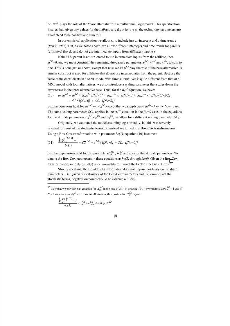
error terms in the three alternative case. Thus, for the α R Ld equation, we have:
(10) ln α R Ld
= α 0 Ld
+ α shift Ld
I[N d >0] + α Time Ld ⋅ t ⋅ I[N d >0] + α Time
Ld ⋅ t ⋅ I[N d =0]⋅ SC d
+ ε Ld { I[N d >0] + SC d ⋅ I[N d =0]}
Similar equations hold for α R Md and α R
Kd , except that we simply have α R Kd
=1 in the N d =0 case.
The same scaling parameter, SCd, applies in the α R Md equation in the N d =0 case. In the equations
for the affiliate parameters α R Ld , α R
Md and α R Kd , we allow for a different scaling parameter, SC f .
Originally, we estimated the model assuming log normality, but this was severely
rejected for most of the stochastic terms. So instead we turned to a Box-Cox transformation.
Using a Box-Cox transformation with parameter bc(1), equation (10) becomes:
(11)( ) Ld Ld
bc Ld R x
bcε α
α +=
−)1(
1)1(
{ I[N d >0] + SC d ⋅ I[N d =0]}
Similar expressions hold for the parameters Md Rα , Kd
Rα and also for the affiliate parameters. We
denote the Box-Cox parameters in these equations as bc(2) through bc(6). Given the Box-Cox
transformation, we only (mildly) reject normality for two of the twelve stochastic terms.15
Strictly speaking, the Box-Cox transformation does not impose positivity on the share
parameters. But, given our estimates of the Box-Cox parameters and the variances of the
stochastic terms, negative outcomes would be extreme outliers.
15 Note that we only have an equation for Kd Rα in the case of N d > 0, because if Nd = 0 we normalize
Kd Rα = 1 and if
N f = 0 we normalize α R Kf = 1. Thus, for illustration, the equation for
Kd Rα is just:
( ) Kd
d Kd time
Kd 0
)3( bc Kd R SC t aa
)3( bc
1ε
α ⋅+⋅+=
−

7/29/2019 MNC Related Doc
http://slidepdf.com/reader/full/mnc-related-doc 21/82
19
Turning to the correlations of the ε , we specify that
(12) ( )′ Nd Md Ld ε ε ε ~ ( )d N Σ,0 ,
where Σ d is unrestricted. Similarly, for affiliates, Σ f is unrestricted. But, in order to conserve on
parameters, we do not allow for covariances between the parent and affiliate share parameters.16
Finally, consider the TFP parameters H d and H f in equations (1) and (2). Since we do not
observe output prices and quantities separately, we cannot identify the scale of the H (either
absolutely or for the affiliate relative to the parent. However, we can identify technical progress.
Thus we normalize H d = H f = 1 at t=0 (1983) and let each have a time trend:
(13) H jt = (1 + h j )t
for j=d,f .
We could not reject a specification with equal time trends, so we set hd = h f = h.
III.3.B. Demand Function Parameters
Now, we turn to the stochastic specification for the demand function parameters. For the inverse price elasticity of demand, or market power, parameters, g 1 and g 2, we specify:
( )
( )2
1
g shift 2,time ,220
8bc2
g shift 1,time ,110
7 bc1
0]·I[Nf g t g g )8( bc
1 g
0]·I[Nd g t g g )7 ( bc
1 g
ε
ε
+>+⋅+=−
+>+⋅+=−
(14)
and, for the demand function intercepts, we specify:17
(15)
2d 0
1 f 0
2 f 0
1d 0
P 2shift 0d,
2time ,d 0
20 ,d 0
)12( bc2d 0
P 1shift 0f,
1time , f 0
10 , f 0
)11( bc1 f 0
P 2 shift 0f,
2time , f 0
20 , f 0
)10( bc2 f 0
P 1shift 0d,
1time ,d 0
10 ,d 0
)9( bc1d 0
0]·I[Nf P t P P )12( bc
1 ) P (
0]·I[Nd P t P P )11( bc
1 ) P (
0]·I[Nf P t P P )10( bc
1 ) P (
0]·I[Nd P t P P )9( bc
1 ) P (
ε
ε
ε
ε
+>+⋅+=−
+>+⋅+=−
+>+⋅+=−
+>+⋅+=−
16 Interpretation of the Σ d and Σ f terms is rather subtle. The logistic transformation already incorporates the negative
correlation among the share parameters that is generated by the CRTS assumption. If Σ d = I , we have an “IIA”setup, where if one domestic share parameter increases, the other share parameters decrease proportionately. The
correlations in Σ d and Σ f allow firms to depart from this IIA situation. For example, if Σ d 12 is very large, then we get
a pattern where firms with large domestic labor shares also have large domestic materials shares.17 Technically, we should impose that g 1 and g 2 are positive and less than 1, and that the P o terms are positive.Equations (14)-(15) do not impose these constraints. But, given our estimates, violations would be extreme outliers.

7/29/2019 MNC Related Doc
http://slidepdf.com/reader/full/mnc-related-doc 22/82
20
Preliminary estimations of the model suggested that cross correlations between the 3 groups of
parameters (technology, price elasticities, and demand function intercepts), were not important.
Also, allowing for all possible cross correlations leads to a substantial proliferation of
parameters, which, in turn, leads to extreme difficulty in obtaining convergence of the search
algorithm. Thus, we specified 1 g ε and 2 g ε as independent of other stochastic terms and allowed
the ) , , ,( 2d 0
1 f 0
2 f 0
1d 0 P P P P
ε ε ε ε vector to be correlated within itself but not with the other stochastic
terms. We denote the covariance matrix of the latter vector by Σ P .
III.3.C Labor Force Adjustment Cost Parameters
Recall that labor force adjustment costs are given by equation (6). The parameters δ d and δ f are
allowed to vary across firms as follows:
(16) { } ]0 N [ I t wexp dt d d dt d 0 ,1d dt >⋅+⋅++= δ δ δ δ δ
]0 N [ I t wexp ft f f ft f 0 ,1 f ft >⋅+⋅++= δ δ δ δ δ
As with the other structural parameters, we allow for the possibility that adjustment costs vary
over time, and we allow for the possibility that the adjustment costs differ between firms that do
and do not have intra-firm flows. We also allow the δ to be functions of the wage rate, on the
premise that search and severance costs for high wage/highly skilled labor are higher).
III.3.D Serial Correlation
Since we have a panel, it is important to allow for serial correlation of the errors within each firm
over time. We specify a permanent-transitory (random effects) structure. Thus, e.g, for the
stochastic part of the parent labor share parameter ε Ld we have:
)()()( it Ld i Ld it Ld ν µ ε += for t=1,…T i
and similarly for the other eleven parameters. Let µ i ∼ N(0, Σ µ ) denote the 12×1 vector of random
effects for firm i, and let ν it ∼ N(0, Σ ν ) denote the 12×1 vector of firm/time specific error
components. Then, V t ≡ Var( ε it ) = Σ µ + Σ ν and C t-j, t ≡ Cov( ε it , ε i,t-j ) = Σ µ . Note that Σ µ and Σ ν
each contain 78 unique elements, but these are restricted as described earlier. For instance, the
non-zero elements of Σ µ + Σ ν consist entirely of elements of P f d , Σ Σ Σ and along
with 21 g σ and 2
2 g σ . Other cross-correlations are set to zero. Defining ) ,....,( iiT 1ii ε ε ε = we have:
(17)
=
ii T T 1
212
1
i
V C
V C
V
)( Var
!!
"#ε
So far, we have only considered the most general case where a firm has all 4 potential trade
flows. If a firm has N dt =0 (or N ft =0) at time t , then there is no value for ε Kd (it) (or ε Kf
(it)).
7/29/2019 MNC Related Doc
http://slidepdf.com/reader/full/mnc-related-doc 23/82
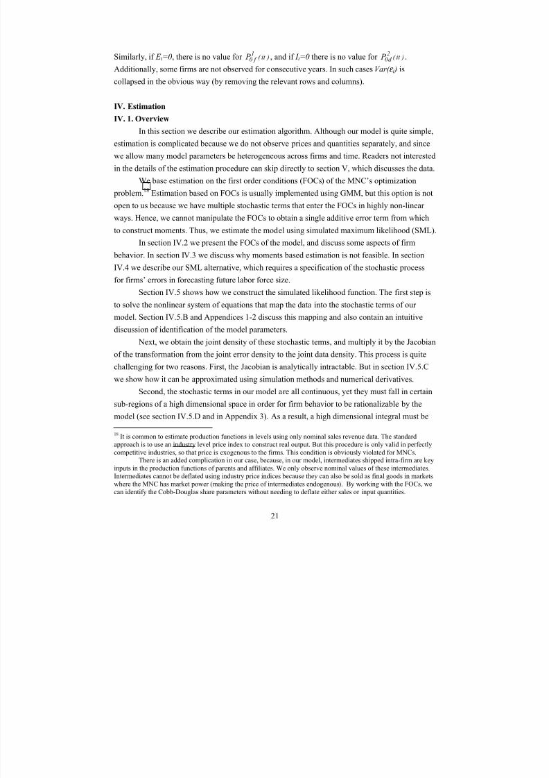
21
Similarly, if E t =0, there is no value for )it ( 1 f 0 P , and if I t =0 there is no value for )it (
2d 0 P .
Additionally, some firms are not observed for consecutive years. In such cases Var( ε i ) is
collapsed in the obvious way (by removing the relevant rows and columns).
IV. Estimation
IV. 1. Overview
In this section we describe our estimation algorithm. Although our model is quite simple,
estimation is complicated because we do not observe prices and quantities separately, and since
we allow many model parameters be heterogeneous across firms and time. Readers not interested
in the details of the estimation procedure can skip directly to section V, which discusses the data.
We base estimation on the first order conditions (FOCs) of the MNC’s optimization
problem.18 Estimation based on FOCs is usually implemented using GMM, but this option is not
open to us because we have multiple stochastic terms that enter the FOCs in highly non-linear
ways. Hence, we cannot manipulate the FOCs to obtain a single additive error term from which
to construct moments. Thus, we estimate the model using simulated maximum likelihood (SML).
In section IV.2 we present the FOCs of the model, and discuss some aspects of firm
behavior. In section IV.3 we discuss why moments based estimation is not feasible. In section
IV.4 we describe our SML alternative, which requires a specification of the stochastic process
for firms’ errors in forecasting future labor force size.
Section IV.5 shows how we construct the simulated likelihood function. The first step is
to solve the nonlinear system of equations that map the data into the stochastic terms of our
model. Section IV.5.B and Appendices 1-2 discuss this mapping and also contain an intuitive
discussion of identification of the model parameters.
Next, we obtain the joint density of these stochastic terms, and multiply it by the Jacobian
of the transformation from the joint error density to the joint data density. This process is quite
challenging for two reasons. First, the Jacobian is analytically intractable. But in section IV.5.C
we show how it can be approximated using simulation methods and numerical derivatives.
Second, the stochastic terms in our model are all continuous, yet they must fall in certain
sub-regions of a high dimensional space in order for firm behavior to be rationalizable by the
model (see section IV.5.D and in Appendix 3). As a result, a high dimensional integral must be
18 It is common to estimate production functions in levels using only nominal sales revenue data. The standardapproach is to use an industry level price index to construct real output. But this procedure is only valid in perfectlycompetitive industries, so that price is exogenous to the firms. This condition is obviously violated for MNCs.
There is an added complication in our case, because, in our model, intermediates shipped intra-firm are keyinputs in the production functions of parents and affiliates. We only observe nominal values of these intermediates.Intermediates cannot be deflated using industry price indices because they can also be sold as final goods in marketswhere the MNC has market power (making the price of intermediates endogenous). By working with the FOCs, wecan identify the Cobb-Douglas share parameters without needing to deflate either sales or input quantities.

7/29/2019 MNC Related Doc
http://slidepdf.com/reader/full/mnc-related-doc 24/82
22
evaluated to construct the joint density of a firm’s stochastic terms. In section IV.5.E and
Appendix 4 we present a recursive importance sampling algorithm that can deal with this
integration problem. The algorithm is the discrete/continuous analogue of the GHK algorithm
(see, e.g., Keane (1994)) for discrete choice data. Just as GHK has found wide application in
discrete choice problems, the new algorithm may have wide application in discrete/continuous
problems. For instance, it would be useful in any situation where, in certain regions of the space
of stochastic terms, a firm would shut down or discontinue certain activities, etc., and where one
needs to simulate the density of marginal decisions conditional on the firm being active.
Evaluating our model’s distributional assumptions (as well as simulation of the model) is
also challenging. To do this we need a practical way to draw ex-post from the joint distribution
of the model’s stochastic terms, given our estimates. The vector of stochastic terms is 14×1, but
is constrained to lie in a 12 dimensional sub-space determined by the12×1 data vector. In section
IV.6 and Appendix 5 we present another new GHK type algorithm to draw a K
×1 vector of
continuous random variables subject to the constraint it lie in a space of dimension less than K.
Finally, in section IV.7 and Appendix 6 we present the reduced form heterogeneous logit
model that we use to model firms’ decisions about whether to engage in each of the four possible
trade flows. We allow for both heterogeneity and state dependence in these decisions using a
new approach recently suggested by Wooldridge (2001).
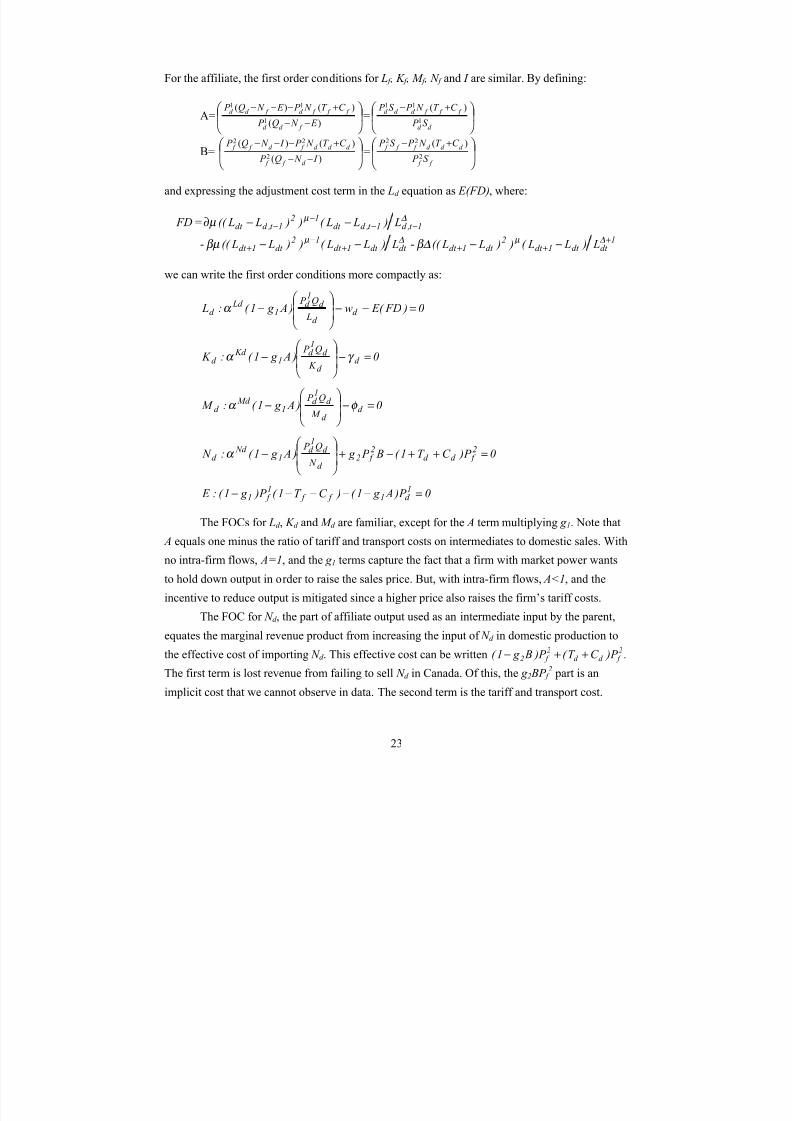
IV.2. Solution of the firm’s problem and Derivation of Estimable FOCs
The first order conditions for parent factor inputs and parent’s exports to Canada are:
0:
)1(
)(
)()(
1
111
1
1
=
−−−
−
∂
∂
∂
∂
−−
+−−− +
d
d
d
d
d f d d
f f f d f d d
d
d d Ld
d
d d Ld
d L
AC
L
AC
E N Q P
C T N P E N Q P
L
Q P
L
Q P
E w g L β α α
0:)(
)()(
1
111
1
1
=−
−
−−
+−−−d
f d d
f f f d f d d
d
d d Kd
d
d d Kd
d E N Q P
C T N P E N Q P
K
Q P
K
Q P g K γ α α
0:)(
)()(
1
111
1
1
=−
−
−−
+−−−d
f d d
f f f d f d d
d
d d Md
d
d d Md
d E N Q P
C T N P E N Q P
M
Q P
M
Q P g M φ α α
−
−−
+−−−
) E N Q( P
)C T ( N P ) E N Q( P
N
Q P
N
Q P
f d 1d
f f f 1d f d
1d
d
d 1d Nd
1d
d 1d Nd
d g : N α α
0 P )C T 1( P g 2 f d d
d f 2
f
d d d 2
f d f 2
f 2 f 2
) I N Q( P
)C T ( N P ) I N Q( P =++−
+
−−
+−−−
0)1()1(: 1
11
111
1
1
)(
)()(=−−−+
+
−−+−−−
f f f f d d
f f f d f d d
d d C T P g P g P E E N Q P
C T N P E N Q P
7/29/2019 MNC Related Doc
http://slidepdf.com/reader/full/mnc-related-doc 25/82

7/29/2019 MNC Related Doc
http://slidepdf.com/reader/full/mnc-related-doc 26/82
24
Similarly, the first order condition for E equates the marginal revenue from exports of the
domestically produced good to Canada with the marginal revenue from domestic (U.S.) sales.
Observe that if the Canadian tariff and transport costs are zero, ( C f + T f ) = 0, then A = 1. As a
result, the FOC for E reduces to P f 1= P d
1, which means that the MNC exports the domestically
produced good to the point where price in the US and Canada are equalized.
Tariffs and transport costs create a wedge between the U.S. and Canadian prices for final
goods. For instance, if the affiliate does not use the good produced by the parent (good 1) as an
intermediate input, then A=1, and the FOC for exports reduces to P d 1 /P f
1= (1-T f -C f )<1. Thus,
Canadian tariff and transport costs cause good 1 to cost more in Canada.19 However, if the
affiliate uses good 1 as an intermediate, then A<1. The parent then has an incentive to hold down
P d 1
because the tariff and transport cost of shipping intermediates to Canada is increasing in P d 1.
This effect is stronger the less elastic is demand (i.e., the larger is g 1) and the higher are tariffs.20
Since prices and quantities are not separately observed, we cannot take these FOCs
directly to the data. We now describe how we can manipulate the FOCs to obtain estimable
equations that contain only observed quantities and unknown model parameters. First, if we
multiply each first order condition by the associated control variable, we obtain:
0 L ) FD( E Lw )Q P )( A g 1( : L d d d d d 1d 1
Ld d =−−− δ α
0 K )Q P )( A g 1( : K d d d 1
d 1 Kd
d =γ −−α
(18) 0 M )Q P )( A g 1( : M d d 1
d 1 Md
d =φ−−α
0 ) N P )( C T 1( B ) N P ( g )Q P )( A g 1( : N d 2
f d d d 2
f 2d 1
d 1 Nd
d =++−+−α
0 ) E P )( A g 1( )C T 1 )( E P )( g 1( : E 1
d 1 f f 1
f 1 =−−−−−
Note that in the first order condition for E , the endogenous quantity ) E P ( 1d is not observable.21
However, we can exploit the fact that:
(19) ) E P ( 1d = ) E P ( 1
f 1 f
1d
P
P
= ) E P ( 1
f
1 g
1 f
d 1d
1 f 0
1d 0
E P
S P
P
P ⋅
−
19 Without our assumption that price elasticity of demand for good 1 is equal in both countries, the price ratio wouldalso depend on the difference in demand elasticities. But with equal elasticities, the incentive to raise price byreducing sales is equally strong in both countries, so price is equalized except for the tariff and transport cost wedge.20 If the parent tries to lower P d
1 too much relative to P f 1 it might create an arbitrage opportunity whereby third
parties could buy the good in the U.S. and resell it in Canada. We could invoke a segmented markets (or no resale)condition as in Brander (1981) to rule out this possibility. Such an assumption is common in trade models withdifferentiated products. Alternatively, we could assume transport costs are higher for third parties.21 Note: P d
1 E is the physical quantity of exports times their domestic (not foreign) price – an object we cannotconstruct since we do not observe prices and quantities separately
7/29/2019 MNC Related Doc
http://slidepdf.com/reader/full/mnc-related-doc 27/82
25
to express the first order condition for E in terms of observable quantities and the ratio of
demand function intercept parameters )1 f 0
1d 0 P P as follows:
(20) E: 0 ) E P ( ) A g 1( )C T 1 )( E P )( g 1( 1 f
1 g
1
f
d 1d
1
f 0
1d 0
1 f f 1
f 1 E P
S P
P
P =⋅
−−−−−
−
Similarly, in the FOCs for the factor inputs, the quantity )Q P ( d 1
d is also not observed. We
can rewrite this quantity as ( ) ) E P ( P P N P S P Q P 1 f
1 f
1d f
1d d
1d d
1d ++= but, again, E P 1d is not
observed. We therefore repeat the same type of substitution to obtain, for domestic labor:
(21) 0 L ) FD( E Lw ) E P ( N P S P ) A g 1( : L d d d d 1
f
g
1 f
d 1d
1 f 0
1d 0
f 1d d
1d 1
Ld d
1
E P
S P
P
P =−−
++−
−
δ α
The FOCs for K d , M d and N d are obtained similarly, so we do not repeat them. The FOCs for the
affiliate have a similar form.
We now have ten first order conditions ( Ld , K d , M d , N d , L f , K f , M f , N f , E , I ) expressed in
terms of observable quantities, unknown parameters, and an unmeasured expectation term.
Below, we show how these FOCs can be used to identify the Cobb-Douglas share parameters,
the price elasticities of demand, and the ratios of the demand function intercepts for the two
goods – i.e., ( )1 f 0
1d 0 P P and ( )2
f 02d 0 P P . We will need price indices for capital and materials in
order to identify the demand function intercepts separately (and the TFP terms). It is important to
note however, that an important subset of parameters, and hence some of our key results, are
identified without needing to deflate any of the nominal quantities we observe in the data.
IV.3. The Choice of Estimation Method
We could in principle use nonlinear GMM to estimate our model using the ten FOCs
derived in section IV.2, along with a sufficiently large set of instruments to identify all the model
parameters. Since a GMM approach is so commonly used for estimation based on FOCs, we first
describe why it is not feasible for our model. Then we describe our SML approach.
To illustrate the problems with GMM, it is useful to consider a simpler stochastic
specification than that in section III.3. Consider the Ld equation (21), which contains threestochastic terms (α it
Ld , g 1it and 1
d 0 P / 1 f 0 P ). Suppose we specify that:
)it ( Ld Ld Ld
it exp ε α α +=
)it ( 1
1it 1 g g exp g +=
( ) { } )it ( 11it
1 f 0
1d 0 pr PRexp P P +=
7/29/2019 MNC Related Doc
http://slidepdf.com/reader/full/mnc-related-doc 28/82
26
Here, we have only imposed that the share parameter for labor be positive. We have not imposed
CRTS. Thus, this specification is simpler than what is needed, but will suffice to make our point.
Next, to deal with the expectation term in (21), we invoke a rational expectations assumption:
(22) d it dit it dit it t L FD L ) FD( E η−=
and obtain the following equation for Ld , incorporating forecast errors, d it η :
(23)
⋅
++−
−−
− ) E P ( ee N P S P ) Aee1 )( e( e: L 1
f
ee
1 f
d 1d )it ( 1 pr 1 PR
f 1d d
1d
g 1 g d
1it g 1 g
1it
Ld it
Ld
E P
S P ε α
0=+−− d it d dit it d d d L FD Lw ηδ δ
The other equations of the model could be obtained similarly, by substituting expression for the
stochastic parameters into the other FOCs.The problem with a GMM approach in this context is obvious. The four stochastic terms,
ε it Ld , ε it
g1, ε it pr1, and ηit
d , appear in (23) in such a highly nonlinear way that it is not possible to
express the equation as a moment condition with a single additive error term. The key pr oblem is
that there are multiple stochastic terms, and also that the ε it g1
term appears in two places.22 If
there were only a single stochastic term that appeared in only one place, we could always find
appropriate transformations so that the FOC could be written in terms of a single additive error.
Krusell, Ohanian, Ríos-Rull and Violante (2000) confronted a problem similar to what
we face here when they estimated a production function that included unobserved quality of skilled and unskilled labor as two latent (stochastic) inputs. Because they had two stochastic
labor quality shocks, both of which entered nonlinearly, along with a forecast error term, the
FOCs of their model could not be written in terms of a single additive error term.
More fundamentally, even if we could implement a GMM approach successfully, it
would not be adequate for our purposes. The usual argument for GMM over ML is that one
avoids making distributional assumptions – in this case on the technology, market power and
demand shift parameters that are assumed heterogeneous across firms, and on the forecast errors
– and thereby obtains more robust estimates of model parameters. But we need to assume (andestimate) the distribution of the firm specific parameters in order to be able to simulate the
response of the population of firms to changes in tariffs or other features of the environment.
22 A second problem is that, even if we could linearize equation (23), the choice of instruments is not at all obvious.Usual candidates like input prices might well be correlated with other firm specific technology parameters if technology changes over time in response to price changes. Third, nonlinear GMM is known to often suffer fromsevere numerical instability, even in much simpler models than this.

7/29/2019 MNC Related Doc
http://slidepdf.com/reader/full/mnc-related-doc 29/82
27
IV.4 The SML Approach, and the Stochastic Process for Forecast Errors
Given the problems with a GMM approach, we decided to estimate the model by
simulated maximum likelihood (SML). SML can deal with the fact that multiple stochastic terms
enter the FOCs in (20)-(21) in a highly nonlinear way. But the use of SML raises a new problem,
which is how to handle the unmeasured expectation term in (21). In a full information ML
approach, one would specify how firms form expectations of future labor inputs. This would
require us to specify how they forecast future demand and technology shocks, tariffs, exchange
rates, etc. This in turn would require us to completely specify the stochastic processes for all
these forcing variables. This would go well beyond the scope of the present investigation.
Our approach is a compromise in which we assume particular parametric distributions for
the demand and taste shocks, as in a full ML approach. But, rather than specifying stochastic
processes for all the forcing variables (e.g., tariffs, exchange rates, etc.), we simply substitute
realizations of the t+1 labor demand terms for their expectations, as in a typical GMM approach.That is, we substitute equation (22) into FOCs like (21) to obtain estimable equations. Then, we
specify distributions of the forecast errors, ηit d and ηit
f , and estimate the model using SML.23
Krusell et al (2000) adopted a similar approach. Their model contained an unmeasured
expectation of next period’s price of capital. Since they used parametric likelihood methods to
estimate their model (for reasons discussed in IV.3) they also had to specify a forecast error
distribution. They assumed normality. We also assume normality for the forecast errors in our
model (equation (22)). But we generalize the Krusell et al (2000) approach by showing how to
test the distributional assumption. We also relax normality by using a Box-Cox transformation,
and we show how to implement SML (Krusell et al used a simulated pseudo-ML procedure).
In terms of what we can do with our model once it is estimated, our approach also
represents a compromise between the full solution ML approach and the GMM approach. Since
we estimate the complete distribution of technology and demand parameters for the MNCs, we
can do steady state simulations of the responses of the whole population of firms to changes in
the tariffs and other features of the environment. But, since we do not model the evolution over
time of all the forcing processes, we cannot simulate transition paths to a new steady state.
Without loss of generality we rewrite (22), the equation for forecast errors, as follows:
(24)d
it dit it dit it L FD L ) FD( E η+= *dt dt dit it L FD ησ +=
where *dt η is standard normal. We tried applying a Box-Cox parameter in (24) rather than
assuming normality for *dt η . But the estimated Box-Cox parameter was extremely close to one.
23 It is worth emphasizing that the key difficulty in estimating our model arises not from the dynamics, but rather from the nonlinear way in which the set of stochastic terms that capture firm heterogeneity enter the FOCs. This problem would still be present even if we eliminated labor force adjustment costs and estimated a static model.

7/29/2019 MNC Related Doc
http://slidepdf.com/reader/full/mnc-related-doc 30/82
28
As we’ll see, the distribution of the forecast errors appears to be strikingly well described by
normality. Clearly, we expect that σ dt , the standard deviation of the domestic labor adjustment
cost forecast error, will be an increasing function of Ldit , so we write:
(25) { }dt 10d dt Lexp τ τ σ +=
ft 10 f ft Lexp τ σ τ +=
Regarding serial correlation, we assume that the forecast errors are independent over time, as
implied by rational expectations. But we allow parent and affiliate forecast errors to be correlated
within a period, as must be the case if their production processes are integrated, or if they face
common shock components. Thus, we let ( )′ f d ηη ∼ N(0 , Σ η ). We also let Σ η = CC ′ , where C
is the lower triangular Cholesky decomposition
2212
11
C C
0C . Finally, let τ = ( τ d0 , τ f0 , τ 1 ).
IV.5 Construction of the Simulated Likelihood FunctionIV.5.A Overview
To construct the likelihood function, we need two things: 1) the mapping from the
observed data for a firm to the set of firm specific parameters that rationalize the data, and 2) the
Jacobian of the transformation from the joint density of the stochastic terms to the joint density
of the data. In this section we consider these two problems in turn.
Suppose we wish to evaluate the likelihood function at a particular trial parameter value.
This includes values for the common (or non-stochastic) parameters of the model, which are R,
β , δ d , δ f , µ , ∆, τ and h, and also for the parameters of the joint distribution of the 12 firm specific
stochastic terms (see section III.3). Further suppose we have draws for the forecast errors, ηd and
η f , in hand. (We discuss how to obtain these draws below). Then, we can use the ten first FOCs
(see equations 20-21), and the production functions (1) and (2) to solve for the 12 stochastic
terms for each firm and time period. Next, calculate the joint density of the stochastic terms and
multiply by the Jacobian to obtain the data density. Repeating this process at independent draws
for ηd and η f , and averaging the data densities obtained in each case, we obtain a simulation
consistent estimator of the likelihood contribution for the firm.
IV.5.B Solving for the Error Terms (and Identification of the Model Parameters)
Solving the system of 12 nonlinear equations for the 12 stochastic parameters in themodel is cumbersome. We describe the details in Appendix 1. Here we give a brief summary:
The market power parameters g 1 and g 2 are identified by simple markup relationships
(i.e., Lerner conditions), which we can construct using data on sales revenues and costs. These
relationships are modified slightly to account for labor force adjustment costs, and also for the
complication that the MNC has an incentive to hold down prices of final goods it ships intra-firm

7/29/2019 MNC Related Doc
http://slidepdf.com/reader/full/mnc-related-doc 31/82
29
as intermediates (in order to avoid tariff costs). The U.S./Canadian price ratios for goods 1 and 2,
denoted PR1 and PR2, are determined by the tariff and transport cost wedge, again modified by
the incentive to hold down prices of intra-firm intermediates. Since the strength of this incentive
depends only on g 1 and g 2, we can solve for PR1 and PR2 once g 1 and g 2 are obtained. Also, given
g 1 and g 2, the Cobb-Douglas share parameters are identified by cost shares of modified revenues.
Finally, given g 1 and PR1, we can infer the ratio of the U.S. to Canadian demand function
intercepts for good 1 (i.e., P 0d 1 /P 0f
1) by observing the ratio of U.S. to Canadian sales for good 1.
Similarly, by comparing affiliate sales in Canada vs. imports to the U.S., we can infer the ratio of
domestic to foreign demand function intercepts for good 2 (i.e., P 0f 2 /P 0d
2).
Thus, without separate data on prices and quantities (other than wages and employment,
which we need only because we estimate the labor force adjustment cost function), we can use
the 10 FOCs of the model identify the market power parameters g 1 and g 2, the Cobb-Douglas
share parameters, and the ratios of the demand function intercepts for good 1, P 0d 1 /P 0f
1, and good
2, P 0f 2 /P 0d
2. To identify the levels of the demand intercepts, we need capital and materials price
indices. Then, we can separate price and quantity for the capital and materials inputs, and utilize
the production functions (1)-(2) as additional equations to determine quantities of output.24
Having solved for all the firm specific parameters, we use the equations of the stochastic
specification (see section III.3) to construct the vector of error terms for the firm. Let ε it denote
the vector of (up to) 12 error terms for firm i in period t (or, as few as 8 if N d = N f = E = I = 0):
ε it ≡ ( ε it Ld
, ε it Md
, ε it Nd
, ε it Lf , ε it
Mf , ε it
Nf , ε it
g1 , ε it
g2 , ) , , ,
2d 0
1 f 0
2 f 0
1d 0 P
it P
it P
it P
it ε ε ε ε
Finally, we construct the joint multivariate normal density of the error vector for firm i, which
we denote by ε i ≡ ( ε i1 , … , ε iT(i) ), where T(i) is the number of time periods that firm i is observed,
using the covariance structure given by equation (17).
IV.5.C The Jacobian of the Transformation from the Error to the Data Density
Of course, the likelihood is the joint density of the data, not of the stochastic terms. We
now turn to the construction of the Jacobian. If yi denotes the vector of data elements for firm i,
then )(||)( iiii f y y f ε ε ∂∂= where ii y∂∂ε is the Jacobian of the transformation from the data
to the stochastic terms. In our case, the 12 data items observed for the firm (or as few as 8 if N d =
N f = E = I = 0) at time t are:
{ } f f d d 2
d 1
f f 1
d d 2
f f f d d f d f 2
f d 1
d it M , M , I P , E P , N P , N P , Lw , Lw , L , L ,S P ,S P y φ φ =
Observe that the Jacobian is not block diagonal by period t , because ε it is affected by Ld,t-1, L f,t-1,
24 Appendix 2 augments Appendix 1 by giving an intuitive explanation of how the time trends in TFP (h) and in thedemand function intercepts (the P 0) are separately identified, and how the profit rate is identified. To the extent thatgrowth is more than proportionately slower for firms with more market power, it implies that growth is induced byTFP rather than growth in demand. The profit rate governs the relationship between market power and capital share.

7/29/2019 MNC Related Doc
http://slidepdf.com/reader/full/mnc-related-doc 32/82
30
Ld,t+1 and L f,t+1. It is not possible (as far as we can determine) to obtain an analytic expression for
the Jacobian, because the mapping from the data to the stochastic terms is so highly nonlinear.
Furthermore, the mapping depends on the values of the forecast errors (which we condition on
here, but which must be integrated out). Therefore, we construct the Jacobian numerically.
To calculate the numerical Jacobian we bump the elements of the data vector (y) one at a
time. When a data element is bumped, we recalculate all the elements of ε i, and form numerical
derivatives of ε i with respect to that element of y. We then use these numerical derivatives to fill
in the column of the Jacobian that corresponds to the bumped element of y. We have:
∂∂⋅⋅⋅⋅⋅⋅∂∂
⋅⋅
⋅∂∂
∂∂
⋅⋅⋅⋅∂∂
∂∂
=
12 ,iT
12 ,iT
1 ,1i
12 ,iT
1 ,1i
2 ,1i
12 ,iT
1 ,1i
2 ,1i
1 ,1i
1 ,1i
1 ,1i
ii
i
ii
i
y y
. y
y y y
) y ,( J
ε ε
ε
ε ε ε
η
where yitk denotes the k th element of the data vector for firm i in year t . For instance, if we bump
yi11= )1i( d 1
d S P , and form numerical derivatives of the ε i elements, we obtain the first column of
the Jacobian. We denote the Jacobian J( ηi , yi ) to highlight that it depends on the forecast errors.
IV.5.D Simulating the Likelihood Function: Naïve Approach
We form the likelihood by integrating the data density over the forecast error distribution:
L iiii
N
1i
d ) f( ) ,| y( f )(
i
ηηθ ηθ
η
Π ∫ =
=
iiiiiiii
N
1i
d ) y ,( f )| ) y ,( ( f ) y ,( J
i
ηηθ ηε ηη
Π ∫ =
=
Here, , ) ,....., ,( f
iiT d
iiT f 1i
d 1ii ηηηηη ≡ f (ηi ) denotes the joint density of forecast errors for firm i, and
θ denotes the vector of model parameters. The notation ε i ( ηi , yi ) emphasizes that the mapping
from the data to the stochastic terms for a firm depends on the vector of forecast errors ηi.
Naively, we could simulate the likelihood function by taking iid draws from the
distribution of ηi. An important complication arises here, however. Firm behavior cannot be
rationalized by any arbitrary values for the forecast errors. Conditional on a particular draw for
(ηd , η f ), firm behavior is only rationalizable if, when we solve the mapping from the data to the
model parameters, we obtain 1>g 1 > 0 , 1>g 2 > 0, all technology parameters positive, and all
demand shift parameters positive. But this will not be the case for all possible (ηd , η f ) draws.

7/29/2019 MNC Related Doc
http://slidepdf.com/reader/full/mnc-related-doc 33/82
31
In Appendix 1 we derive the following equation relating g 1 and the forecasts E(FD)Ld :
(26) B ) N P ( L ) FD( E CD RD ] AYE [ g d 2
f BVI
) L ) FF ( E CF RF ( d d BVI
) N P )( N P ( AB1
f f d 2
f f 1
d δ δ
−−+−−=−
In our data, the term BVI / ) N P )( N P ( AB AYE d 2
f f 1d
− is always positive.25 So, the right-hand
side of (26) must be positive in order for g 1 to be positive. But if the forecasted adjustment costs
E(FD) = FD - ηd or E(FF) = FF - η
f are too large, the right-hand side will be driven negative.
Thus, observed firm behavior implies bounds on the forecast errors. We derive the bounds on
(ηd , η f ) in Appendix 3.
For any draw (ηd , η
f ) that does not satisfy the bounds, no values of the firm specific
parameters can rationalize firm behavior. Let BDi denote the region of the space of forecast
errors such that behavior of firm i is rationalizable. Then, we can rewrite the likelihood as:
1i BD
iT iiiii BD
N
1i d ...d ) f( ... ) f( )| ) y ,( ( f ) y ,( J .......... )iiT iiT
i
1i1i
ηηηηθ ηε ηθ ηηΠ ∫ ∫ ∈∈==( i1iTi
L
1iiT iiiii
N
1i
d ...d ) f( ....... ) f( ] BD[ I ....... ] BD[ I )| ) y ,( ( f ) y ,( J ...i
iiT 1i
ηηηηηηθ ηε ηηη
Π i1iTi1i1iTiT iii∫ ∈∈∫ ==
where I[ ηit ∈ BDit ] is an event indicator. Then, given M iid draws from the unconditional
distribution of the forecast errors, the likelihood contribution for firm i can approximated using a
simple frequency simulator as follows:
(27) ] BD[ I ... ] BD[ I )| ) y ,( ( f ) y ,( J M )( ˆ iT
m
iiT m1ii
mii
M
1m
imi
1
ii1i ∈∈∑==
− ηηθ ηε ηθ L
There are two fundamental problems with this approach, however:
1) For some draws m, the likelihood contribution is zero. For example, suppose P( ηit ∈ BDit ) =
.95 ∀ t and there are 11 periods. Then only 56% of draws would belong to BDi on average.
This creates a serious numerical inefficiency, since many draws are useless for evaluating the
|J( ηi ,yi )| f (ε i( ηi ,yi )|θ ) term. They are only used (implicitly) to evaluate event probabilities
P( ηi ∈ Β Di ), which could be much more accurately evaluated by other means (see below).
2) The simulated likelihood in (27) is not a smooth function of the model parameters θ . It takes
discrete jumps at θ values such that one of the draws miη is exactly on the boundary of Β Di.
This means that gradient-based search algorithms cannot be used to maximize the likelihood
function, and derivatives are not available to calculate standard errors of parameter estimates.
25 A and B are usually close to 1. Therefore, AYE is close to sales of good 1, and BVI is close to sales of good 2 (seeAppendix 1 for definitions). Thus, the second term includes ( P f
2 N d / BVI ), a number < 1, times P d 1 N f , which is just
one component of sales of good 1. So the whole term in brackets is roughly sales of good 1 minus a fraction thereof.

7/29/2019 MNC Related Doc
http://slidepdf.com/reader/full/mnc-related-doc 34/82
32
IV.5.E A Recursive Importance Sampling Approach
We implement a more efficient smooth simulator of the likelihood using a recursive
importance sampling algorithm that is a discrete/continuous data analogue of the GHK algorithm
for simulating event probabilities in discrete choice models. As in GHK, the idea is to draw the
ηi from the “wrong” density, chosen so that all ηi with positive mass under this density are
consistent with firm behavior. The likelihood is then simulated using a weighted average over
these draws, where the weights are ratios of the likelihood of a draw under the correct density
f (ηi) to the likelihood of a draw under the incorrect density f( ηi | ηi ∈ Β Di ). We describe the
implementation of the algorithm in Appendix 4.
Define BDt as the region in which (ηt d , ηt
f ) must fall in order for firm behavior to be
rationalizable in year t . Then, as described in Appendix 4, we obtain the following smooth
unbiased simulator for the likelihood contribution of firm i:
| BD( P ) BD( P .... )| BD( P ) BD( P )| ) y ,( ( f ) y ,( J M )( ˆ T fT T dT
m1d 11 f 11d i
mii
M
1mi
mi
1iiii
ηηηηηηθ ηε ηθ ∈∈⋅⋅∈∈∑==
−iL
Since many economic models have a structure where certain stochastic terms must be in
particular ranges in order for a continuous outcome to be observed, the basic approach used here
can be useful in many contexts. Since the simulator is recursive it can be extended trivially to
accommodate serial correlation in the ηt . The bounds for η2 would then be a function of m1η , and
so on. We rule out such correlation here because of the forecast error interpretation of η.
IV.6 Testing Distributional Assumptions
Our model contains a 14×1 vector of stochastic terms for each firm and time period (i.e.,
12 firm specific parameters, and two forecast errors). We assume this vector is multivariate
normal. But drawing from its posterior distribution conditional on firm behavior is a nontrivial
problem. The 12×1 vector of data elements places complex constraints on the 14×1 vector of
stochastic terms. Appendix 5 describes the recursive importance sampling algorithm that we use
to draw the stochastic terms. We use these draws to test the normality assumption.
IV.7 The Firm’s Decision Rules for Import, Export, and Intra-Firm Trade Activities
We also estimate reduced form approximations to MNCs’ decision rules for whether to
utilize each of the four potential trade flows. We condition on these decisions in our structural
estimation, which could lead to endogeneity bias if they are influenced by firm specific
unobservables. To accommodate this, our structural estimation is fully simultaneous with our
estimation of the reduced form decision rules for the four trade flows. We allow firms’ capital
share and market power parameters to enter the rules, which we specify as logits. Tariffs, wages
prices and exchange rates are also included as covariates.
Das, Roberts and Tybout (2001) estimated a structural model of firms’ decisions to
7/29/2019 MNC Related Doc
http://slidepdf.com/reader/full/mnc-related-doc 35/82
33
export. In their model, there is a fixed cost of commencing export activity. As noted by Bernard
and Jensen (2001), fixed costs generate state dependence in reduced form export decision rules.
We allow for both state dependence and unobserved firm heterogeneity, and use a new procedure
due to Wooldridge (2001) to deal with the initial conditions problem that arises in such models.
The basic idea is to let the firm effect be correlated with the initial decisions and the initial tariff
level. For a detailed exposition of our logit decision rules see Appendix 6.
V. Data
V.1 Construction of the Panel
Our data are from the Benchmark and Annual Surveys of U.S. Direct Investment Abroad
administered by the Bureau of Economic Analysis (BEA). These confidential surveys contain the
most comprehensive information available on the activities of U.S.-based MNCs and their
foreign affiliates. They contain observations for every U.S. MNC with one or more affiliates
(above a specified size). The BEA collects data separately from parents and affiliates, which can
be merged using an identifier for the parent.
For this study, we use the BEA data on U.S. MNCs with one or more Canadian affiliates,
disaggregated at the individual foreign affiliate level. The sample period is 1983-1996. Overall,
this sub-sample contains 24,313 affiliate-year observations.
We made several alterations to the original BEA data to construct our panel data set.
First, note that the BEA classifies firms into roughly 120 2-3 digit ISI industry codes, of which
50 are manufacturing industries. Since many non-manufacturing industries produce non-
tradeables (i.e., retailing, real estate and hotels), we use only data on manufacturing affiliates.
This screen reduced the total number of affiliate-year observations from 24,313 to 12,241.
Second, we must assign each affiliate to an industry, in order to match it with the
appropriate tariff and transport cost data. The large majority of affiliates are not diversified, so
the appropriate assignment is clear.26 There were, however, cases that appeared to be spurious
changes in industry classification, or where affiliates consistently had less than 80% of sales in a
single industry. We dropped such cases, leading to a loss of 1677 affiliate-year observations.
Third, it is important to note that the Benchmark and Annual Surveys have different
coverage. The Benchmark Surveys, conducted in 1977, 1982, 1989 and 1994 include the whole
population of MNCs and their foreign affiliates. But, in the Annual Surveys, the smaller affiliates
are exempt from filing. If an affiliate reports data in a Benchmark Survey but is exempt from the
Annual Surveys, the BEA carries it forward by estimating data. As a result, most of the data for
26 On average 91% of Canadian manufacturing affiliate sales were in only one industry. The median affiliate sells alloutput in one industry. By contrast, only 65% of U.S. parent sales were in one industry.

7/29/2019 MNC Related Doc
http://slidepdf.com/reader/full/mnc-related-doc 36/82
34
smaller affiliates in non-Benchmark years is estimated rather than reported.
Ideally, we would remove all the estimated data. However, our panel data analysis relies
on having several consecutive observations on parent/affiliate pairs. In particular, recall that we
need lead and lag data to deal with labor force adjustment costs, so an affiliate must be observed
for three consecutive years to contribute one observation to our analysis, four consecutive years
to contribute two observations, etc. We did not want to lose several observations for an affiliate
because just a few of its observations were estimated.
As a compromise, the decision rule we used in this step was: 1) remove all observations
for affiliates that did not have at least three consecutive reported observations, and 2) keep
estimated observations for the remaining affiliates only if they were bracketed at t-1 and t+1 by
valid reported observations.27 This procedure led to the elimination of most of the estimated data
(altogether, we removed 4247 affiliate-year obser vations in this screen).
This left 6358 affiliate-year observations.28 Data were removed several more times to
arrive at the final sample. First, same industry affiliates of the same parent were combined,
reducing the sample to 5583 affiliate-year observations. Second, data were removed because of
missing affiliate or parent data for sales, employment or employee compensation. Third,
observations that were not elements of a string of three consecutive observations were removed.
This left a total of 5175 firm-year observations on 551 parents and 716 affiliates in our sample.
Our model abstracts from the possibility that an MNC might have multiple Canadian
affiliates. For our purposes, we care about how changes in tariffs and other factors affect the
allocation of the MNC’s production and trade activities between the U.S. and Canada, and not
the organizational form of the MNC’s Canadian operations. Therefore, if a parent had multiple
affiliates we merged them into a single “composite” affiliate in two steps. First, if the parent had
multiple affiliates in the same industry, we merge them into a composite affiliate, simply by
adding up the employment, sales, etc. of the individual affiliates. Second, if the parent had
affiliates in multiple industries, we take only the largest, based on total sales. This size
comparison is done after the merging of same industry affiliates in step one.
Finally, our model does not allow for the possibility that an affiliate would have no
domestic sales in Canada (this is a very rare event in the data). We deleted 8 cases of parent-
affiliate pairs where the affiliate had zero Canadian sales. After this step, our final data set
contained 3385 unique affiliate-year observations on 543 unique parents and affiliates.
27 For example, suppose an affiliate had a string of observations 11011011101101 over the fourteen years of data,where a “1” denotes a reported observation, and a “0” denotes estimated data. If we keep all the estimatedobservations, this affiliate contributes 12 valid data points, but if we drop all estimated observations, it contributesonly 1 valid data point. Under our procedure, we would keep all observations for this affiliate, since each estimatedobservation is bracketed by two valid reported observations.28 There are 41 observations that would have been removed by both the second and third screens.
7/29/2019 MNC Related Doc
http://slidepdf.com/reader/full/mnc-related-doc 37/82
35
It is important to emphasize that our analysis sample contains only manufacturing
affiliates. This is important, because in our model we assume that intermediates shipped between
the parent and affiliate are goods destined for further processing. Such an assumption would
obviously be invalid if we included, for instance, wholesale and retail trade affiliates.
V.2 Construction of Variables
The BEA data contain U.S. parents’ domestic sales, affiliates’ domestic sales (in
Canada), the value of intermediates shipped intra-firm (in both directions), and affiliates’ arms-
length sales to the U.S.. These are five of the six key sales variables in our model. Unfortunately,
we do not directly observe US parents’ arms-length sales to Canada. To construct arms-length
sales to Canada, we used data from Compustat on total parent sales to Canada, and subtracted out
the value of intra-firm shipments from parents to Canadian affiliates.29
We also need measures of capital, labor and materials inputs. The BEA data contain
information on employment and the wage bill for both parents and affiliates. We use the ratio of
these variables as our measures of wage rates, which are assumed to be specific to each parent
and affiliate.30 This is the only instance where we observe separate data on price and quantity.
To construct measures of materials input, we used information on cost of goods sold
(CGS). For affiliates, the BEA data contain direct information on CGS. We calculate affiliate
materials input by subtracting the wage bill, imports from U.S. parents, and current depreciation
from CGS. U.S. parents do not report CGS, so we needed to obtain this item from Compustat. 31
As discussed in section III.2, we constructed the payments to capital inside our estimation
algorithm, since we did not feel there were reliable measures of payments to capital for parents
and affiliates in the BEA data. The BEA data do include property plant and equipment (PPE) at
historical cost, and such measures are often used to construct payments to capital (by assuming a
required rate of return and a depreciation rate). However, given the well-known limitations of
historical PPE data, we preferred to implement our new procedure, described in section III.2 and
Appendix 2, of estimating a profit rate and backing out payments to capital as a residual.
Interestingly, our residual measures turned out to be highly correlated with PPE.
All data on nominal quantities (i.e., sales, trade flows, costs of labor and materials inputs)
were put in real terms using the U.S. GDP deflator (results were little changed by using the CPI
29
If Compustat data were not available, we assumed that a given parent’s ratio of arms-length to intra-firm exportswas the same for Canada as for other countries. Then, we multiplied U.S. parent intra-firm exports to Canadianaffiliates by the parents overall (i.e., worldwide) ratio of arms-length to intra-firm exports (which is contained in theBEA data). But if the U.S. parent had zero sales to the affiliate, this formula could not be used. In these cases, wemultiplied a U.S. parent’s total (worldwide) arms-length sales by the ratio of Canadian to worldwide arms-lengthsales for all U.S. parents (obtained from the Benchmark Survey published data).30 That is, each firm requires a particular type of labor (e.g. a particular skill level), with its own specific wage rate.31 Since cusip numbers are not regularly reported by US parents in the BEA data, we generally used the name of the parent firm to match up the BEA and Compustat data. For parents with no Compustat data, we used the averagevalue of the CGS to Sales ratio for their industry to calculate CGS.

7/29/2019 MNC Related Doc
http://slidepdf.com/reader/full/mnc-related-doc 38/82
36
or PPI instead). The BEA instructs firms to report Canadian values in current US dollars, so we
did not need to make any exchange rate adjustment. We implicitly assume that firms use the
nominal U.S./Canada exchange rate to do the conversion.
Our use of the GDP deflator amounts to an assumption that the MNC’s objective is to
maximize the present value of profits in GDP-deflated U.S. dollar terms. It is crucial to note that
this assumption has no implication for the within period producer prices of capital, labor and
materials. This is because we estimate firm specific demand functions, implying firm specific
output prices. The ratio of nominal input prices to these firm specific output prices determines
producer prices. Our choice of price deflator only comes into play when the firm considers how
its current period labor input will affect future labor force adjustment costs. Firms are assumed to
evaluate these future costs in GDP-deflated U.S. dollar terms.
As we discussed in Section IV.5.B, all the parameters of our model except the levels of
the demand function intercepts are identified without needing measures of real capital and
materials inputs. But to identify these intercepts in levels we need to measure real inputs. To put
materials costs in real terms, we use, for U.S. parents, the BLS producer price index (PPI) for
intermediate supplies, materials and components for manufacturing, and for Canadian affiliates,
the PPI for manufacturing intermediates, obtained from Statistics Canada. For the cost of capital
we use the price index for gross private domestic (non-residential) investment in producer
durables from the BLS. The cost of capital is assumed to be the same in the U.S. and Canada.32
Key variables of interest in our model are tariffs and transport costs. We measure U.S.
and Canadian tariffs on an ad valorem basis for each of our 50 manufacturing industries. That is,
the tariff on imported goods in industry j in year t is measured as the ratio of duties paid to the
value of the imports. A measure of transportation costs was constructed by dividing the industry-
level cost of insurance and freight by the total value of imports in each industry j at time t .33
Although these tariff and transport cost measures are more aggregated than the level at which
tariffs are actually imposed, they are more disaggregated than measures often used in empirical
work (see Grubert and Mutti, 1991).
As shown in Figure 1, U.S. and Canadian tariffs fell substantially over the 1983-1996
32 The assumption that the price of capital is the same in both countries is motivated by the assumption that the
required rate of return on capital is equalized across the MNC as a whole, and that the MNC can raise funds for allits operations in international capital markets. But our assumption also requires that real prices of physical capitalmove in sync over time in each country. Substantial relative movements of the price of physical capital would createarbitrage opportunities if capital goods can be shipped across the border. Implicitly, we are assuming that transportcost is a trivial fraction of total cost for capital goods but not for materials inputs (whose real price we do allow todiffer across the two countries). This assumption on transport costs is reasonably accurate.33 U.S. tariff and transportation cost data were obtained from the Census Bureau. Canadian tariff data were obtainedfrom Statistics Canada. Canadian tariffs were reported at the three-digit SIC code level, which were converted intoUS SIC codes, then BEA ISI codes. Transportation cost data for imports into Canada was not available fromStatistics Canada, so we simply assumed that these costs were the same as for imports into the U.S..

7/29/2019 MNC Related Doc
http://slidepdf.com/reader/full/mnc-related-doc 39/82
37
period. Canadian tariffs fell from an average of nearly 6% to 1.75%, and U.S. tariffs fell from
4% to less than 1%. There is also considerable cross-industry variation in tariffs. U.S. tariffs are
highest in tobacco (average 13%) and lowest in motor vehicles and pulp and paper (average less
than 0.2%). Canadian tariffs are highest in tobacco and apparel (both averaging over 17%), and
lowest in agricultural chemicals, autos and farm machinery (all averaging approximately 1%).
Since the affiliates in our data are predominantly single-industry, it was straightforward
to assign then the appropriate U.S. tariff and transport cost data. For diversified U.S. parents, we
constructed sales-weighted average Canadian tarif f and transport cost measures across the (up to)
eight industries in which U.S. parents report sales.34
VI. Empirical Results
VI.A. Descriptive Statistics
Table 1 gives descriptive statistics for the firms in our sample. To estimate our structural
model, we need one-period lags and leads of the labor force data in order to construct current and
future labor force adjustment costs. Thus, although our panel extends from 1983-1996, we use
data from 1983 and 1996 only to model labor adjustment costs. Table 1 reports summary
statistics on the “complete” data set (which includes 1983 and 1996), and also the “analysis” data
set that only includes the data from 1984-1995 that the model attempts to fit.
In the complete data set, parents’ intra-firm sales to the Canadian affiliates make up 35%
of affiliates’ total sales (which average about 275 million in 1984 US$). Affiliates’ intra-firm
sales to parents are 39% of affiliate total sales. These figures imply a high degree of integration
of the production processes of parents and affiliates. Note that Canadian affiliates’ intra-firm
sales to U.S. parents are larger, on average, than U.S. parents’ sales to Canadian affiliates.
Table 1 also reports the fraction of firms that utilize each of the four trade flows. In the
complete data set, affiliate arms-length sales to the U.S. are positive for 42% of firm-year
observations, while affiliate intra-firm sales to parents are positive 75% of the time. For parents,
the fraction with arms-length sales to Canada is 86%, and the fraction with intra-firm sales to the
affiliate is 82%. These percentages are quite stable over time, despite tariff reductions.
Table 2 provides descriptive statistics on the cost shares for labor, materials and capital. It
reports mean and median cost shares for the firms in the analysis sample. Statistics are presented
for three-year intervals, because there is some noise in the means and medians induced by the
rather frequent entry and exit of small firms from the data set.
34 Note that, in Figures 3-4, Canadian tariffs actually increase slightly for firms in the fourth quartile. This is becausewe construct weighted average tariffs for U.S. parent flows to Canada. A change in the industry mix of sales maylead to an increase in our tariff measure, even if industry level tariffs are decreasing. This is an unavoidableconsequence of the need to aggregate sales and tariffs across industries.

7/29/2019 MNC Related Doc
http://slidepdf.com/reader/full/mnc-related-doc 40/82
38
Our model with Cobb-Douglas technology implies that cost shares should be stable over
time, except for minor fluctuations induced by labor force adjustment costs (see equation A1.13).
In Table 2 we assume zero profits and measure the capital share as the residual of revenues
minus other factor costs. This is not exactly consistent with our model, in which firms have
market power and have positive profits. Thus, in Table 2, the capital share may appear to change
simply because the price elasticity of demand facing firms is changing.
Nevertheless, Table 2 provides evidence that cost shares were quite stable for those
parents and affiliates that did not use intermediates. Given the large movements in relative factor
prices apparent in Figure 2, this suggests that a Cobb-Douglas specification is reasonable. For
instance, between 1984-86 and 1990-92, the price of labor in Canada rose roughly 20% relative
to the prices of materials and capital. Yet, for affiliates that did not use intermediate inputs from
parents ( N f =0), the mean labor share rose only 0.6 percentage points (about 2.4%) over this
period. Thus, unit elastic demand does not seem like too bad an assumption. Input cost shares
also seem stable for parents that do not use intermediates shipped from the affiliate ( N d =0).
But cost shares were much less stable for affiliates that use intermediates from parents.
For such affiliates, the mean (median) capital share dropped from 28.1% (27.5%) in 1984-86 to
21.2% (21.2%) in 1993-95. At the same time, the mean (median) cost share for intermediates
shipped from the parent rose substantially, from 15.0% (9.8%) in 1984-86 to 18.9% (13.6%) in
1993-95. These figures understate the growth in intermediate shares, because there was rapid
growth in both the first and last three years of the sample. Taking a three-year average dampens
this out. Figure 6 makes the rapid growth in affiliates’ intermediate input shares more obvious.
Figure 6 also shows that the share of intra-firm intermediates in parents’ costs increased
by roughly 230% over the sample period. At the same time, parents that use intermediates
shipped from affiliates ( N d >0) had downward trending labor shares. Prima facie, it appears quite
implausible that the drop in the mean U.S. tariff rate from about 3.8% in 1984 to 1.2% in 1995
could explain this huge increase in intermediates shipped from affiliates. This tariff decline
decreased the cost of intermediates to parents by only about 2.5 percent. Thus, enormous demand
elasticities would be needed to rationalize the observed increase in affiliate-to-parent flows of
intermediates on this basis. A similar story holds for parent-to-affiliate flows of intermediates.
VI.B. Parameter Estimates for the Structural Model
Table 3 reports estimates of our structural model of MNCs’ marginal production and
trade decisions. Our smooth SML algorithm (based on 50 draws) was numerically very well
behaved and converged without difficulties in about 300 iterations (that required several minutes
each). Results were not affected when we tried alternative starting values.
The first panel of Table 3 reports estimates of parameters related to the labor share in the
parent’s Cobb-Douglas production technology. Recall that these parameters map into the share

7/29/2019 MNC Related Doc
http://slidepdf.com/reader/full/mnc-related-doc 41/82
39
parameter itself through the transformation given by equations (8), (10) and (11). The estimates
in Table 3 are for the parameters in equation (10). The first term is the intercept (α 0 Ld ). The
second term, α shift Ld , is a shift parameter that allows the labor share to differ for the subset of
firms with positive intra-firm flows (i.e., it multiplies I[N d >0]). The third and fourth terms are
time trends, which are relevant for parents that do and do not use intermediate inputs from the
affiliate, respectively. Finally, the fifth term is the Box-Cox parameter from equation (11) that
captures departures of the stochastic term in the labor share equation from log normality (bc(1)).
The second and third panels of Table 3 report parameters relevant to the parent’s
materials and capital shares, respectively. Note that the capital share equation has fewer
parameters. When a parent does not utilize intermediates from the affiliate, it has only three
inputs, so the capital share is just 1-α Ld -α Md . Thus, the capital share equation is only relevant for
parents that do use intermediates from the affiliate, and so it does not include the shift parameter
or the extra time trend that are included in the labor and material share equations. The fourth
through sixth panels of Table 3 contain exactly the same types of parameters, but for the affiliate.
A fascinating aspect of the results is that the time trends on the share parameters are small
and insignificant for parents and affiliates that do not use intermediates that are shipped intra-
firm. That is, in Table 3, the terms α Time Ld ⋅t ⋅ I[N d =0], α Time
Md ⋅t ⋅ I[N d =0], α Time L f ⋅t ⋅ I[N f =0] and
α Time Mf ⋅t ⋅ I[N f =0] are all insignificant and quantitatively small. Thus, the behavior of these
parents and affiliates is well described by a CRTS Cobb-Douglas technology with fixed share
parameters, consistent with the descriptive statistics on cost shares presented in Table 2.
In contrast, for the subset of MNC parents that do utilize intermediates from affiliates,
and affiliates that use intermediates from parents, the time trends for the share parameters are all
highly significant. The direction of all the trends is negative, but this result should be interpreted
with care. Since the trends feed into logistic transformations like (8)-(9), it is only the share of
the input with the largest negative time trend that necessarily falls. The behavior of shares for
inputs with smaller negative trends is ambiguous. Clearly, however, the fact that the time trends
are negative for labor, capital and materials means the share of the omitted category
(intermediates) must be rising. Thus, conditional on MNCs having had positive intra-firm flows
initially, the estimates imply that technical change was driving up the share of intermediates.
For parents, the strongest negative time trend is on the labor share, while for affiliates it’s
on the capital share. This is consistent with the descriptive statistics in Table 2, which showed
that the labor share trended down for parents while the capital share trended down for affiliates.
For all the technology parameters, the Box-Cox parameters (i.e., bc(1) through bc(6)) are
(slightly) less than zero, implying that a transformation function (slightly) more strongly concave
than the log is necessary to bring them into line with normality.
The next panel of Table 3 contains estimates of the two scale parameters, SC d and SC f

7/29/2019 MNC Related Doc
http://slidepdf.com/reader/full/mnc-related-doc 42/82
40
which account for the fact that the scale of the parameters and stochastic terms in the logistic
equations (8)-(9) that determine shares is not comparable across the three-outcome ( N d = 0, N f
= 0) and four-outcome ( N d > 0, N f >0) specifications. As expected both parameters are less than
one, since the scale should be reduced in the three-outcome case.
The bottom panel on the first page of Table 3 reports estimates of some key parameters of
the model that are common across firms. The estimated profit rate R is16.5% and estimated rate
of TFP growth, h, is 4.5%. We could not reject a specification in which h was common across
the parent and affiliate. Both of these estimates seem reasonable. The high rate of TFP growth
for U.S. MNCs is consistent with prior work in this area (see Cummins (1998)), and the profit
rate estimate seems reasonable given prior estimates (see, e.g., Fraumeni and Jorgenson (1980)).
The top four panels on the second page of Table 3 contain estimates of the labor force
adjustment cost parameters. The estimates for δ d w and δ f w are both close to one, implying that
the cost of a given change in the labor force increases one-for-one with the wage rate. It is
reasonable that search costs are higher (as are severance costs) for high-wage, high-skill workers.
The intercept shift for N f >0 is significant and positive in the δ f equation, suggesting that labor
force adjustment costs are greater for affiliates that ship intermediates to parents. (A dummy for
N d >0 was not significant in this equation, and similarly, a dummy for N f >0 was not significant in
the parent adjustment cost equation). The time trends in the δ d and δ f equations are both
significant and positive, suggesting that labor force adjustment costs increased over time.
The third panel contains estimates of the generalized labor force adjustment cost
function. The estimates of µ and ∆ imply that adjustment costs are not well described by the
common linear-quadratic in levels specification, since they depart substantially from µ =1 and
∆=0. The fact that µ <1 and ∆>0 implies that the cost of a given absolute change in labor force
size is smaller to the extent that the change represents a smaller fraction of the initial labor force.
That is, adjustment costs are determined by something in between the squared absolute labor
force size change and the percentage labor force size change.
The fourth panel contains estimates of the parameters that determine the variance of labor
adjustment forecast errors (τ ). Not surprisingly, the forecast error variances are an increasing
function of labor force size. Interestingly, the domestic forecast error variance is higher (for a
given labor force size), and domestic and foreign forecast errors are positively correlated.
The middle two panels on the second page of Table 3 contain estimates of the parameters
that determine the (negative) inverse price elasticities of demand for the U.S. and Canadian
produced good ( g 1 and g 2). These market power parameters are estimated with an intercept shift
and a differential time trend for firms that use intra-firm flows. Note that the intercept shift is not
significant for either the domestic or foreign market power parameter. Also, the domestic market
power does not vary significantly over time. But market power for Canadian produced goods
7/29/2019 MNC Related Doc
http://slidepdf.com/reader/full/mnc-related-doc 43/82
41
trends downward. The Box-Cox parameter for g 1 implies that a transform close to the square root
is needed to induce normality of the residuals, while the transform for g 2 is closer to linear.
Finally, the last four panels of Table 3 contain estimates of the four demand function
intercept parameters (i.e. U.S. and Canadian demand for the U.S. and Canadian produced goods).
All four demand function intercepts exhibit significant negative time trends, implying reduced
demand at any given price level. The Box-Cox transform parameters for these four equations are
all close to zero, implying that the demand shocks are well described by log normality.
Recall that we allow the technology and demand function parameters to be heterogeneous
across firms and over time. Each of these 12 parameters has a firm/time specific component that
consists of a random effect, µ i, and a transitory error, ν it . Appendix 8 reports estimates of the
correlation matrices of these stochastic terms. Panel 1 presents the cross-sectional correlation
matrix of the composite error µ i+ν it . Although all correlations are highly significant, the smallest
(about 0.4) are for the country specific demand shifters across the two different goods (i.e.,
between 1d 0 P and 2
d 0 P , and between 1d 0 P and 2
f 0 P ). By contrast, the correlation between the U.S.
and Canadian demand shifters for the domestically produced good (i.e., between 1d 0 P and 1
f 0 P ) is
0.97! That is, demand for the same good across the two countries is extremely highly correlated,
while demand for the two different goods in the same country is not so highly correlated.
Panel 2 of Appendix 8 reports correlations of the firm specific parameters at time t and
t+1. The random effects structure implies equal correlations at all leads and lags, all the way out
to t+11. As we would expect, all the firm specific parameters are highly serially correlated. The
technology and demand function intercept parameters show more persistence (i.e., correlations in
the 0.72 to 0.80 range) than do the market power parameters (i.e., correlations of 0.46 and 0.53).
VI.C. Fit of the Structural Model
Our model appears to fit the data quite well, in the sense that our assumptions about the
distributions of the stochastic terms appear (for the most part) to be strongly supported. As we
discussed in section IV.3, we assume the stochastic terms are normally distributed, subject to a
Box-Cox transformation. In order to investigate the validity of this assumption, we used the
importance sampling algorithm of Appendix 5 to simulate ten vectors of simulated residuals (and
associated importance sampling weights) for each observation in our data. Appendix 7 reports
two different tests of the normality assumption based on these simulated residuals.
Panel 1 presents χ2 tests of normality based on the deciles of the normal distribution.
These tests show that the normality assumption is substantially supported. Indeed, we reject
normality at the 1% level for only one of the 12 residuals—the affiliate materials share—and at
the 5% level, we reject normality only for one additional residual—the parent capital share.35
35 The test statistic is χ2 (9), based upon the deciles of the normal distribution. We bootstrap the critical values todeal with the fact that residuals for a firm are highly serially correlated.

7/29/2019 MNC Related Doc
http://slidepdf.com/reader/full/mnc-related-doc 44/82

7/29/2019 MNC Related Doc
http://slidepdf.com/reader/full/mnc-related-doc 45/82
43
reduced tariff levels were important factors in the MNC’s decisions to ship goods intra-firm or to
engage in export or import activities.
The most important predictors of the decision to ship goods intra-firm or to engage in
import or export activity are the lagged choice, the choice at t=1, and the firm effects. The
bottom panel of Table 4 shows that the firm effects have very large estimated variances.
Essentially, our model says that MNC decisions to engage in intra-firm trade and arms-length
imports and exports are driven primarily by state dependence and unobserved firm specific
characteristics. Tariffs have little effect on these decisions. Thus, the response of MNC-based
trade to tariffs appears to be almost entirely on the intensive rather than the extensive margin.
While is tangential to our main results, we do find a few factors, aside from lagged
choices, that are significant determinants of MNC-based trade. The affiliate capital share is
negatively related to the decision to export intermediates to the parent. The decision to ship
intermediates from parent to affiliate is positively related to parent capital share and negatively
related to affiliate capital share. The affiliate’s market power parameter ( g 2) is positively
associated with the parent’s decision to ship goods intra-firm to the affiliate, but not vice-versa.
In contrast to intra-firm trade, decisions to engage in arms-length trade are not strongly
related to capital intensity. Parent wages are positive and significantly associated with the
parent’s decision to export goods arms-length to Canada. Thus, high-wage U.S. parents are more
likely to export. Affiliate market power is significantly negatively associated with the decision to
ship goods arms-length to the U.S. At first this may seem counterintuitive, but it is consistent
with the conventional wisdom that Canada has comparative advantage in resource based
manufactured goods (see Eden (1998)) which are less easily differentiated.
VII. Simulations of Tariff Effects on Trade
In Table 5 we use simulations of our model to examine the effect of tariff reductions on
MNC-based trade. Specifically, using a steady-state simulation, we compare the baseline levels
of intra-firm and arms-length trade in the last year of our sample (1995), given actual tariffs in
that year, to the levels that would have obtained under two different counterfactual scenarios: (1)
no tariff reductions (i.e., keeping tariffs at their 1984 levels) and (2) complete tariff elimination.
Since we have not implemented a full-solution algorithm,36 we cannot simulate the short-
run outcomes generated by our dynamic model. However, we can use a steady-state version of
our model (which assumes no labor force adjustment costs) to simulate the long-run response of
the population of firms to changes in the policy environment. The simulations are done using 543
36 To do so would require us to specify how expected future labor force size is determined, which in turn wouldrequire specification of the driving processes for demand shocks, tariffs, wages, prices of materials and capital, andtechnical change. All this is well beyond the scope of the paper.
7/29/2019 MNC Related Doc
http://slidepdf.com/reader/full/mnc-related-doc 46/82
44
vectors of technology and demand parameters drawn from the posterior distribution of the firm
specific parameters of our model, obtained using the algorithm described in Appendix 5.
The first row of Table 5 shows the mean levels of domestic sales, intra-firm and arms-
length trade flows and U.S. and Canadian labor that MNCs are predicted to choose (in the long-
run steady state) under the actual policy regime that prevailed in 1995. The second panel shows
the levels that would have obtained under the counterfactual that U.S. and Canadian tariffs are
held fixed at their 1984 levels. And the third row simulates the complete elimination of tariffs. In
each case, the technology and demand parameters are held fixed at their 1995 levels. The
simulations assume that firms only adjust to tariff changes on the intensive margin, since our
estimates imply that tariffs have no significant effect on the extensive margin.
Our simulations imply that arms-length trade is quite sensitive to tariffs. If tariffs were
raised to their 1984 levels, U.S. arms-length exports to Canada would drop 19%, while affiliate
arms-length sales to the U.S. would drop 31%. And our model predicts that complete elimination
of tariffs would increase these arms-length trade flows by about 28% and 21%, respectively.
A key result in Table 5 is the difference in sensitivity of the intra-firm and arms-length
trade flows to changes in tariff levels. For instance, the intra-firm trade flow from U.S. parents to
Canadian affiliates is predicted to drop only about 4% if tariffs were raised back to their 1984
level, and the intra-firm flow from affiliates to parents is predicted to drop only about 2%.
This contrast between a strong effect of tariffs on arms-length trade and a weak effect on
intra-firm trade is consistent with the raw data that we reported in Figures 3-4. There, we saw
that at the industry level there was a rather close relationship between the extent of tariff
reductions and increases in arms-length trade. But there was no obvious relationship between the
extent of tariff reductions and increases in intra-firm trade.
What accounts for the differential sensitivity of arms-length and intra-firm trade to tariffs
in our model? Our model is able to generate rather substantial increases in arms-length trade
from the historically observed tariff reductions (of about 2 to 4 percentage points) because our
median estimates of price elasticities of demand for final goods are –17.6 for the domestically
produced goods and –21.5 for the goods produced in Canada.37 It is worth noting that our model
cannot pick these elasticities just to match tariff effects, since, as we stressed in our discussion of
identification, they are pinned down by revenue vs. cost differentials (i.e., Lerner conditions).
On the other hand, it would be difficult for any model to generate the observed increase
in intra-firm trade based on historical tariff reductions for two reasons: First, the price elasticity
of demand for intra-firm intermediates would have to be implausibly large relative to that for
other inputs. Demands for other inputs appear to be rather close to unit elastic, in light of the
37 These figures are obtained by looking at the posteriors for –1/g1 and –1/g2. Note that these elasticities imply amedian markup of about 5%, which, combined with a capital share of about 30%, gives a profit rate of about 16%.

7/29/2019 MNC Related Doc
http://slidepdf.com/reader/full/mnc-related-doc 47/82
45
rather stable cost shares observed in Table 2. Second, lower tariffs reduce firm costs and may
therefore increase demand for all inputs via a scale effect. But the potential of scale effects to
account for increased factor demands is limited, since the average scale of U.S. MNCs and their
Canadian affiliates actually fell over the sample period (see Table 6 below). Thus, our model
implies that most of the increase in intra-firm trade is due to “technical change,” as reflected in
the upward trends in the share parameters for intermediates that we discussed in Section VI.B.
Although we have highlighted the finding that arms-length trade is much more sensitive
to tariffs than intra-firm trade, it would be incorrect to conclude that intra-firm trade is
insensitive. For example, our model predicts that if tariffs were eliminated completely (starting
from the 1995 baseline), then US parents would ship 6.6% more products to their Canadian
affiliates, affiliates would ship 2.1% more intermediates back to parents, and affiliate
employment would increase 5.6%. These are quantitatively important effects, and they imply
that tariffs continue to be a factor restraining intra-firm trade in some industries.
Table 5 also reports effects of the tariff experiments on employment and sales. When
tariffs are raised to the 1984 level, Canadian affiliate domestic sales and employment fall by
5.6% and 8.5%, respectively. Not surprisingly, U.S. parent domestic sales and labor change less
under the high-tariff regime, with the former dropping by 0.7% and the latter dropping by 1.2%.
As we saw in Figure 2, tariffs were not the only factor that changed substantially during
our sample period. There were also substantial changes in relative wages, and in prices of capital
and materials. And our estimates imply substantial technical change. In Table 6 we decompose
changes in key variables of interest into parts due to tariffs vs. technology vs. wages vs. all other
factors. The first column of Table 6 reports the actual changes in several variables of interest that
occurred from 1984-1995. The second column reports the predicted change from 1984 to 1995 in
the steady state level of each variable, given all changes in the environment. The third, fourth
and fifth columns report the predicted changes due to changes in tariffs, technology and wages,
respectively. The last column reports the combined effect of all other factors.
Of course, the predicted change in steady state levels is not directly comparable to the
change in actuals, since the latter include transition dynamics. However, from a face validity
standpoint it is comforting that the predicted changes line up reasonably well with the actual
changes. Our model predicts that all factors combined led to an increase of 99% in U.S. parent
intra-firm sales to affiliates, and a 79% increase in U.S. parent arms-length sales to Canada. The
actual changes were 73% and 75% respectively. And the model predicts that all factors
combined lead to a 123% increase in affiliate intra-firm sales to parents, and a 9% increase in
affiliates arms-length sales to the U.S.. The actual changes were 95% and 4% respectively.

7/29/2019 MNC Related Doc
http://slidepdf.com/reader/full/mnc-related-doc 48/82
46
Interestingly, the model predicts that tariff reductions alone would have increased
affiliates’ arms-length sales to the U.S. by 32.5%. The model implies that technical change was
also driving up affiliate arms-length sales. Yet, overall, affiliate arms-length sales to the U.S.
only increases 9% in the model simulation and 4% in the data. According to the model, rising
Canadian real wages were a key factor holding down exports to the U.S.. As we saw in Figure 2,
the real wage (in U.S. dollar terms) paid by Canadian affiliates increased by 20% from 1984-
1995. Our model predicts that this reduced affiliates’ arms-length exports to the U.S. by 20%.
Table 6 reveals the important role our model assigns to technical change in increasing
intra-firm trade. Of the 99% increase in parents’ intra-firm sales to affiliates, the model attributes
72 percentage points to technical change. And of the 123% increase in affiliates’ intra-firm sales
to parents, the model attributes 84 percentage points to technical change. The changes attributed
to tariff reductions are only about 10 and 5 percentage points, respectively. While these tariff
effects are not trivial, they are an order of magnitude smaller than the impact of technology.
Finally, a fascinating aspect of both the data and the simulations is the radically changing
nature of the parent/affiliate relationship. Affiliate sales in Canada have been falling at the same
time that shipments to parents have doubled. In Feinberg and Keane (2001) we pointed out that
the growth of affiliate shipments of intermediates to parents was clear evidence that Canadian
manufacturing is not being “hollowed out” by free trade, as many opponents of the FTA had
feared. But Canadian manufacturing affiliates are clearly being transformed into production units
that are more fully integrated into the MNCs’ overall production process. In 1984, sales of
intermediates to parents were about 38% of affiliate total sales. By 1995, this figure had risen to
63%! Our model attributes most of this dramatic change not to tariff reductions, but to
technology.
VIII. Conclusions
In this paper, we estimated a structural model MNC production and trade decisions to
gain insight into the factors causing the substantial observed increase in MNC-based trade
between the U.S. and Canada over the past two decades. Our model implies that bilateral tariff
reductions led to roughly a one-third increase in the volume of arms-length MNC-based trade
between the U.S. and Canada over the 1984-1995 period. On the other hand, tariff reductions can
only account for a 5 to 10% increase in intra-firm trade. Intra-firm trade nearly doubled over this
period, and our model implies that technological change accounted for most of the increase.
We find that almost all the substantial increases in both intra-firm and arms-length MNC-
based trade that occurred from 1984-1995 were on the extensive rather than the intensive margin.
Only a small percentage of MNCs changed their initial status regarding whether or not to engage
in intra-firm or arms-length trade, and tariffs were not significantly related to these decisions.

7/29/2019 MNC Related Doc
http://slidepdf.com/reader/full/mnc-related-doc 49/82
47
Organizing to trade intra-firm involves complex decisions about the organization of
production. Thus, it is not surprising that decisions to begin trading intra-firm are insensitive to
moderate tariff changes. An executive at a Canadian affiliate of a U.S. auto paint manuf acturer,
interviewed as part of this study, discussed the minimal role of tariffs in such decisions:38
When duty rates existed, or tariffs got in the way, when you looked at all the considerations, youreally didn’t save any money [by moving production]. Unless there was a shift in technology whichmade sense in addition to something like the tariff or the duty. You need more than one componentto make it a worthwhile move (1996).
What does the “technical change” that our model says accounts for most of the growth of
intra-firm trade really represent? Over the past two decades, significant advances in operations
and logistics software tools, along with the growth of third party logistics services, have enabled
MNCs to more efficiently segment their production globally, while at the same time reducing
inventory and shipping times. We speculate that such advances may have reduced governance
costs (e.g., by enabling MNCs to outsource many administrative and logistics functions), thus
making it optimal for MNCs to produce more intermediates in-house (see, e.g., Grossman and
Helpman (2002)).
For example, Enterprise Resource Planning (ERP) systems collect and integrate
transactional data within the firm and feed the data into manufacturing scheduling and other
basic business functions such as finance and accounting. ERP systems help firms reduce
inventory by synchronizing upstream and downstream activities both across units of the firm and
between a firm and its customers and suppliers. Advance Planning System (APS) packages use
data collected by ERP systems to optimize production. APS programs produce production and
distribution schedules, taking into account requirements for plant capacity, labor and raw
material availability, distribution facility status and the impact on existing orders (Canadian
Business, 1998). These new technologies have been widely discussed in the business press and
the operations research and logistics literatures (see Taylor, 1999, Xenakis, 1999, Glasse, 2002).
Another important development has been the growth of services offered by third party
logistics providers (3PLs). Traditionally, logistics services such as trucking, warehousing,
regulatory compliance, customs clearance, and after-sales service support have been performed
by different firms, both domestically and internationally. Recently, however, there has been
considerable consolidation in these services, and large 3PLs are increasingly bundling diverse
activities internationally. With reliable single sources for nearly all outbound logistics services,
MNCs have achieved both cost and time savings (Gooley, 1999, 2000, 2002a, 2002b).
In light of these developments, we think that technical change is a plausible explanation
for the increasing share of intra-firm intermediates in the production technologies of both parents
38 More detail on the interview data is available from the authors.
7/29/2019 MNC Related Doc
http://slidepdf.com/reader/full/mnc-related-doc 50/82
48
and affiliates during our sample period.39 But there are alternative explanations. One story is that
the increase is not a real phenomenon, but is rather the result of transfer price manipulation. As
discussed in Eden (1998), U.S. effective corporate tax rates are higher than Canadian rates in
manufacturing (46% vs. 36% in 1995), and this creates an incentive for the MNC to shift profits
to Canada. To do this, the MNC should overprice intermediates shipped from the affiliate to the
parent, and underprice intermediates shipped from parent to affiliate. As noted by Mathewson
and Quirin (1979) tariffs counteract the incentive to overprice shipments to parents. Thus, a U.S.
tariff reduction might lead to higher transfer prices on intermediates shipped from affiliates to
parents. Similarly, a high Canadian tariff provides an incentive for the MNC to underprice
intermediates shipped to the affiliate. A tariff reduction would diminish this incentive, perhaps
inducing the MNCs to increase transfer prices on intermediates shipped from parents to affiliates.
But this transfer price manipulation story for the increase in intra-firm intermediate trade
is implausible for two reasons. First, as we noted in section III.2, MNCs’ ability to manipulate
transfer prices is heavily constrained by U.S. and Canadian tax regulations that require an “arms-
length” pricing standard. In fact, there is little or no solid empirical evidence that MNCs engage
in transfer price manipulation in the U.S.-Canada context (see Eden (1998)). Second, the transfer
price story cannot explain large increases in intra-firm trade in industries where tariffs were
already low or nonexistent prior to the FTA and fell very little over our sample period.
We examined data on real trade quantities to externally validate our finding of substantial
increases in intra-firm trade. The US ITC provides data from the Census Bureau on real trade
quantities at its website (dataweb.usitc.gov). The data are not broken down into arms-length vs.
intra-firm. However, our data indicate that the vast majority of U.S./Canada trade in the
computer and office equipment industry (SIC 357) is intra-firm. This is also the industry with the
second highest volume of intra-firm trade (after autos and auto parts). In SIC 3577 (computer
peripheral equipment and parts) the quantity of U.S. exports to Canada increased 446% from
1989 to 1995, while the quantity of imports from Canada increased 169%. Since we know that
almost all trade in this industry is intra-firm, this is clear evidence that the quantity of intra-firm
trade really did increase substantially. The same is true in other sub-categories of SIC 357.
Finally, we also examined the effects of U.S. and Canadian wages on MNC-based trade.
Our data indicates that real wage rates paid by Canadian manufacturing affiliates increased byroughly 20% over our sample period. Our model implies that affiliate arms-length sales to the
U.S. market would have been 20% greater in 1995 if this increase in labor costs hadn’t occurred.
39 It is possible that the increase in intra-firm trade has occurred in part because MNCs have acquired firms that were previously third party suppliers. This is consistent with our story of technical change reducing governance costs. Butwe find this story implausible because the total sales and employment figures in Table 6 indicate that in terms of both net sales and employment MNCs have been shrinking slightly over our sample period.

7/29/2019 MNC Related Doc
http://slidepdf.com/reader/full/mnc-related-doc 51/82
49
References
Baldwin, J.R., and P. Gorecki. 1986. The role of scale in Canada-U.S. productivity differences.Toronto: University of Toronto Press.
Baldwin, R. E. and G.I.P. Ottaviano, Gianmarco I. P. 2001. Multiproduct Multinationals andReciprocal FDI Dumping. Journal of International Economics, 54, pp 429-448.
Bernard, Andrew and J. Bradford Jensen. 2001. Why Some Firms Export. NBER WP #8349.
Bergoeing, Raphael and Timothy Kehoe. 2001. Trade Theory and Trade Facts. Federal ReserveBank of Minneapolis Research Department Staff Report #284.
Brainard, S.L. 1993. An Empirical Assessment of the Factor Proportions Explanation of Multinational Sales. NBER Working Paper # 4583.
Brainard, S.L. 1997. An Empirical Assessment of the Proximity-Concentration Trade-off Between Multinational Sales and Trade. American Economic Review, 87: 520-544.
Brander, J.A. 1981. Intra-Industry Trade in Identical Commodities. Journal of International Economics, 11(1): 1-14.
Canadian Business. 1998. The Business of Supply Chain Management. November 13.
Caves, R. E. 1982. Multinational enterprise and economic analysis. New York : CambridgeUniversity Press.
Caves, R.E. 1990. Adjustment to International Competition. Ottawa: Canadian GovernmentPublishing Centre.
Cummins, J. G. and R. G. Hubbard. 1995. The Tax Sensitivity of Foreign Direct Investment:Evidence from Firm-Level Panel Data, in Feldstein, M., Hines, J.R., and R. G. Hubbard (eds.)The Effects of Taxation on Multinational Corporations. Chicago, IL: University of ChicagoPress.
Cummins, Jason G. 1998. Taxation and the Sources of Growth: Estimates from United StatesMultinational Corporations. NBER Working Paper #6533.
Das, Sanghamitra, Roberts, Mark and James Tybout. 2001. Market Entry Costs, Producer Heterogeneity, and Export Dynamics. NBER Working Paper #8629.
Davis, D. R. and D. E. Weinstein. 2001. An Account of Global Factor Trade. American
Economic Review, 91(5): 1423-53.
Deardorff, A.V. 1998. Fragmentation in Simple Trade Models. University of MichiganDepartment of Economics working paper 98-11.

7/29/2019 MNC Related Doc
http://slidepdf.com/reader/full/mnc-related-doc 52/82
50
Dixit, Avinash and Gene Grossman. 1982. Trade and Protection with Multistage Production. The
Review of Economic Studies, 49:4: 583-594.
Dunning, J. H. 1975. Economic analysis and the multinational enterprise. New York, Praeger.
Eden, Lorraine. 1998. Taxing Multinationals: Transfer Pricing and Corporate Income Taxationin North America. Toronto: University of Toronto Press.
Eastman, H.C., and S. Stykolt. 1967. The Tariff and Competition in Canada. Toronto:Macmillan.
Feinberg, S. E., Keane, M. P. and M. F. Bognanno. 1998. Trade Liberalization and'Delocalization': New Evidence from Firm-Level Panel Data. Canadian Journal of Economics 31(4): 749-77 .
Feinberg, S. E. and M.P. Keane. 2001. US-Canada Trade Liberalization and MNC Production
Location. The Review of Economics and Statistics, 83(1): 118-132.
Fraumeni, Barbara M. and Dale W. Jorgenson. 1980. Rates of Return by Industrial Sector inthe United States, 1948-76. The American Economic Review, 70(2): 326-330.
Gaston, N., and D. Trefler. 1997. The labour market consequences of the Canada-US Free TradeAgreement. Canadian Journal of Economics, 30: 18-41.
Glasse, J. 2002. Survey –IT: The Supply Chain. The Financial Times. June 19, sup1 p.2.
Gooley, T. B.1999. Service Stars: 3Com relies on logistics to provide world-class post-salesservice to its customers in Latin America. Logistics Management and Distribution Report .June 30, p.36.
Gooley, T.B. 2000. Game Plans for Sale. Logistics Management and Distribution Report .October 1, p. 75.
Gooley, T.B. 2002a. Can Latin America make the grade?. Logistics Management. March 1, p.53.
Gooley, T.B. 2002b. Brave new world for 3PLs?: Kuehne & Nagel's deal with Nortel Networksis truly global in scope. Warehousing Management . March 1, p. 9.
Grossman, Gene and Elhanan Helpman. 2002. Integration versus Outsourcing in IndustryEquilibrium. Quarterly Journal of Economics. 85-120.
Grubert, H. and J. Mutti. 1991. Taxes, Tariffs and Transfer Pricing in Multinational CorporateDecision Making. The Review of Economics and Statistics, 73(2): 285-293.

7/29/2019 MNC Related Doc
http://slidepdf.com/reader/full/mnc-related-doc 53/82

7/29/2019 MNC Related Doc
http://slidepdf.com/reader/full/mnc-related-doc 54/82
52
Mathewson, G.F and G.D. Quirin. 1979. Fiscal Transfer Pricing in Multinational Corporations.Ontario Economic Council Research Series. Toronto: University of Toronto Press.
Rugman, Alan M. 1985a. The Determinants of Intra-industry Direct Foreign Investment . NewYork: St. Martin's Press.
Rugman, Alan M. 1985b. Transfer Pricing in the Canadian Petroleum Industry. In Multinationals
and Transfer Pricing , A. Rugman and L. Eden (eds.), London: Croon Helm, p. 173-192.
Soboleva, Nadia. 2000. Foreign Direct Investment: A Dynamic Model of a Firm’s LocationChoice. Working paper, University of Toronto.
Solow, R. M. 1957. Technical Change and the Aggregate Production Function. The Review of Economics and Statistics, 39(3): 312-320.
Taylor, P. 1999. The Revolutionary Shape of Things to Come: Pivotal Role for Information
Technology Managers. The Financial Times. January 13, Survey Edition p. 1.
Trefler, D. 2001. The Long and Short of the Canada-U.S. Free Trade Agreement. NBER
Working Paper #8293.
Yi, K. M. 2001. Can Vertical Specialization Explain the Growth of World Trade?. Forthcoming, Journal of Political Economy.
Wooldrige, Jeffrey M. 2002. Econometric Analaysis of Cross Section and Panel Data.Cambridge, Mass.: MIT Press.
Xenakis, J. 1999. A Mile Wide and a Mile Deep. CFO. February, 15(2): 57-60.
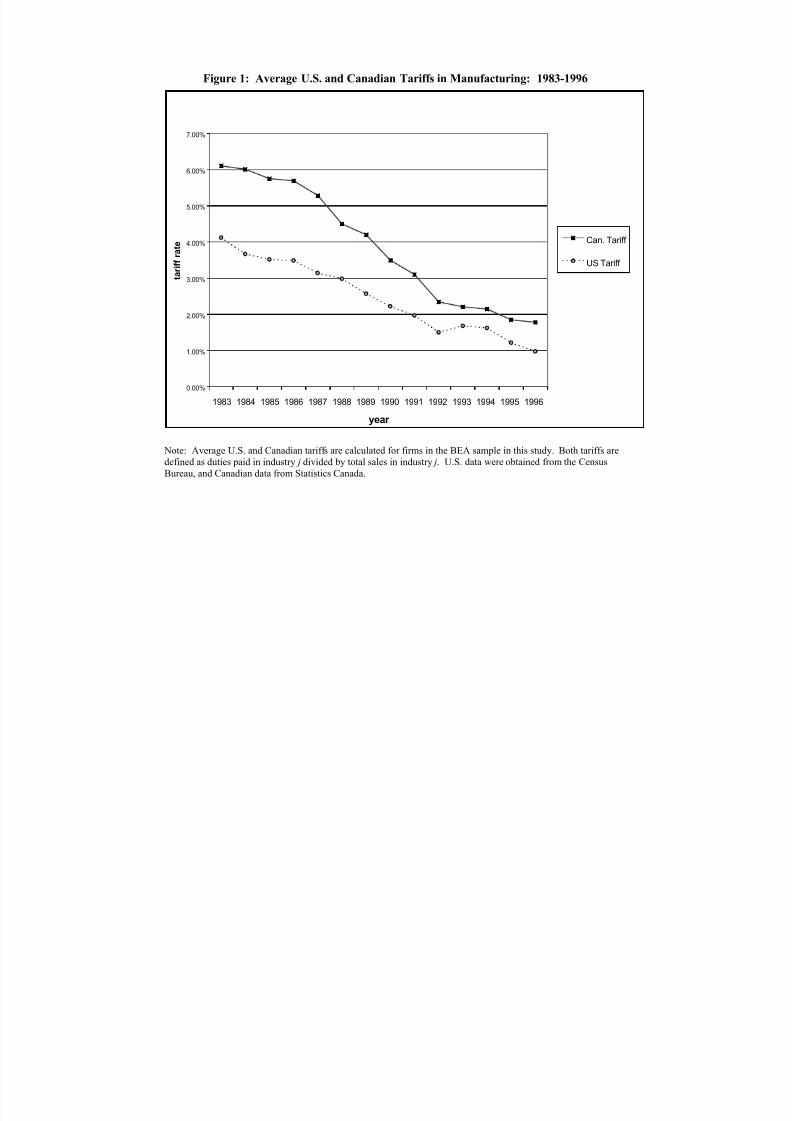
7/29/2019 MNC Related Doc
http://slidepdf.com/reader/full/mnc-related-doc 55/82
Figure 1: Average U.S. and Canadian Tariffs in Manufacturing: 1983-1996
Note: Average U.S. and Canadian tariffs are calculated for firms in the BEA sample in this study. Both tariffs aredefined as duties paid in industry j divided by total sales in industry j. U.S. data were obtained from the CensusBureau, and Canadian data from Statistics Canada.
0.00%
1.00%
2.00%
3.00%
4.00%
5.00%
6.00%
7.00%
1983 1984 1985 1986 1987 1988 1989 1990 1991 1992 1993 1994 1995 1996
year
t a r i f f r a t e
Can. Tariff
US Tariff
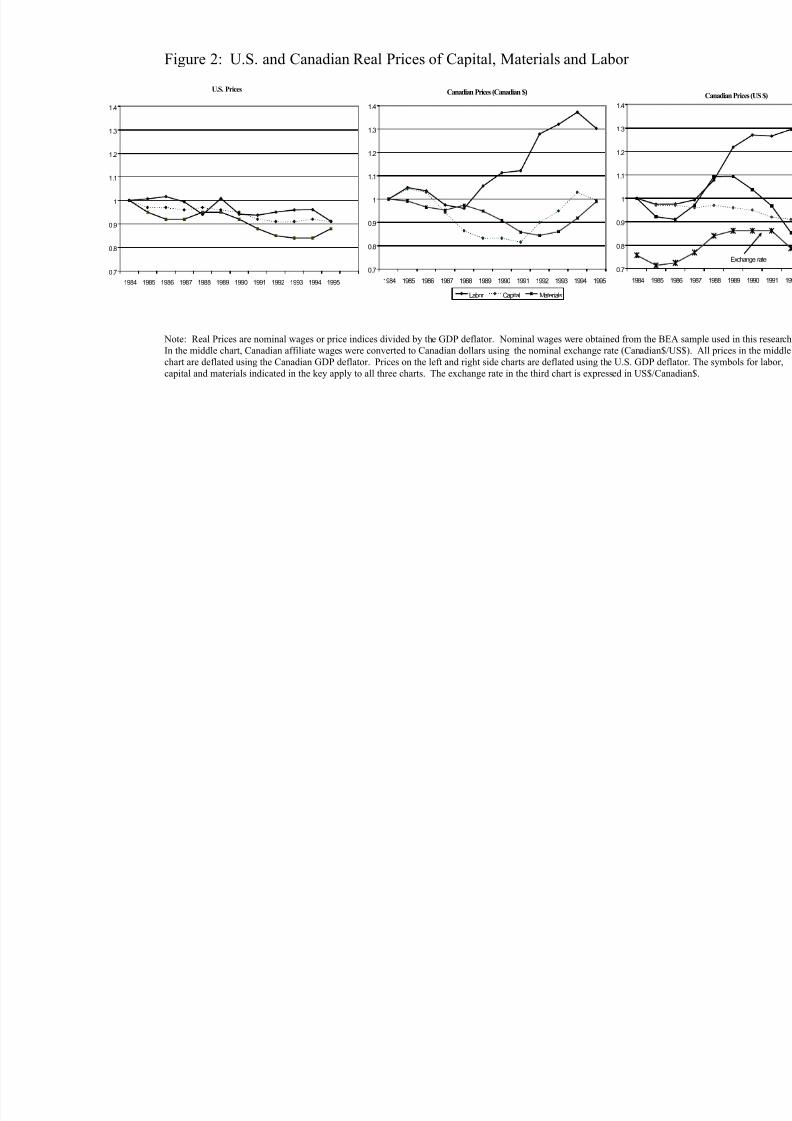
7/29/2019 MNC Related Doc
http://slidepdf.com/reader/full/mnc-related-doc 56/82
Figure 2: U.S. and Canadian Real Prices of Capital, Materials and Labor
Note: Real Prices are nominal wages or price indices divided by the GDP deflator. Nominal wages were obtained from the BIn the middle chart, Canadian affiliate wages were converted to Canadian dollars using the nominal exchange rate (Canadian$chart are deflated using the Canadian GDP deflator. Prices on the left and right side charts are deflated using the U.S. GDP decapital and materials indicated in the key apply to all three charts. The exchange rate in the third chart is expressed in US$/Ca
U.S. Prices
7
8
9
2
3
4
1984 1985 1986 1987 1988 1989 1990 1991 1992 1993 1994 1995
Canadian Prices (Canadian $)
0.7
0.8
0.9
1
1.1
1.2
1.3
1.4
1984 1985 1986 1987 1988 1989 1990 1991 1992 1993 1994 1995
Labor Capital Materials
0.7
0.8
0.9
1
1.1
1.2
1.3
1.4
1984 1985

7/29/2019 MNC Related Doc
http://slidepdf.com/reader/full/mnc-related-doc 57/82
Figure 3: Change in U.S. Parent flows to Canada by changes in Canadian tariffs, 1989-1995
Figure 4: Change in Canadian Affiliate Flows to the U.S. by changes in U.S. tariffs: 1989-1995
Notes: Tariff changes are calculated conditional on each flow being greater than zero in both periods. Tariff changes are in pshown are the medians of each quartile.
Arms-Length Sales to Canada
-20%
-10%
0%
10%
20%
30%
40%
-4.07
<25%
-2.30
25-50%
-1.55
50-75%
0.29
>75%
Percentage point change in Canadian tariff
P e r c e n t c h a n g e i n f l o w
Sales of Intermediates to Canadian Af
-20%
0%
20%
40%
60%
80%
100%
120%
140%
160%
-3.88
<25%
-2.07
25-50%
-0.9
50-75
Percentage point change in Canad
P e r c e n t c h a n g e i n f l o w
Sales of Intermediates to U.S. Pare
0%
20%
40%
60%
80%
100%
120%
-1.91
<25%
-1.02
25-50%
-0.60
50-75%
Percentage point change in U.S.
P e r c e n t c h a n g e i n f l o w
Arms-Length Sales to the U.S.
0%
20%
40%
60%
80%
100%
120%
140%
-1.91
<25%
-0.97
25-50%
-0.43
50-75%
-0.03
>75%
Percentage point change in U.S. tariffs
P e r c e n t c h a n g e i n f l o w
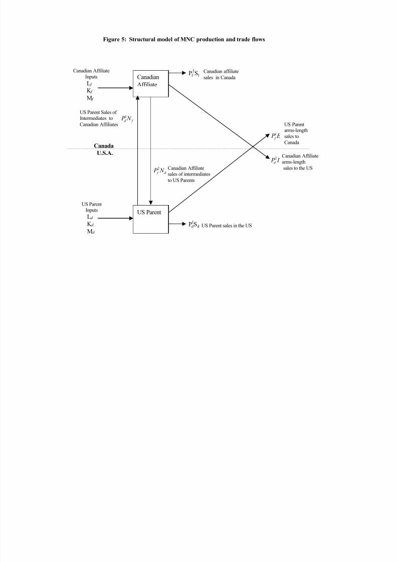
7/29/2019 MNC Related Doc
http://slidepdf.com/reader/full/mnc-related-doc 58/82
Figure 5: Structural model of MNC production and trade flows
US Parent Sales of Intermediates to
Canadian Affiliates
Canadian Affiliatearms-length
sales to the USCanadian Affiliatesales of intermediates
to US Parents
US Parent sales in the US
f
2
f SP
f d N P 1
E P f 1
Canada
U.S.A. I P d
2
d f N P 2
d
1
dSP
US Parentarms-lengthsales to
Canada
Canadian affiliate
sales in Canada
US Parent
CanadianAffiliate
Canadian Affiliate
InputsL f K f
M f
US ParentInputs
Ld K d
Md

7/29/2019 MNC Related Doc
http://slidepdf.com/reader/full/mnc-related-doc 59/82
Figure 6: Average and Median Intermediate Real Input Shares for U.S. Parents and Canadian Af
Notes: Intermediate shares for parents and affiliates are calculated conditional on the shares being greater than zero.
Parent Intermediate Input Shares (mean)
0.0%
0.5%
1.0%
1.5%
2.0%
2.5%
3.0%
3.5%
1984 1985 1986 1987 1988 1989 1990 1991 1992 1993 1994 1995
Affiliate Intermediate Input Share (mean)
12%
14%
16%
18%
20%
22%
1984 1985 1986 1987 1988 1989 1990 1991 1992 1993 1994 1995
Parent Intermediate Inp
0.0%
0.2%
0.4%
0.6%
0.8%
1.0%
1.2%
1.4%
1984 1985 1986 1987 1988 1989
Affiliate Intermediate Inp
6.0%
8.0%
10.0%
12.0%
14.0%
16.0%
18.0%
1984 1985 1986 1987 1988 1989

7/29/2019 MNC Related Doc
http://slidepdf.com/reader/full/mnc-related-doc 60/82
Table 1: Descriptive Statistics ( $ 000’s )
Complete Data Setn=3385
Analysis Data Setn=2335
Mean(St. Dev.)
Mean(St. Dev.)
Canadian Affiliate Flows
Sales in Canada f S 2 f P 156305
(566636)138493(531427)
Sales of Intermediates to US Parents d 2
f N P 108167(740065)
88164(667864)
Percent positive observations 75.2% 71.8%
Arms-Length Sales to US I P d
2 12393
(41440)
10660(38389)
Percent positive observations 41.9% 39.1%
U.S. Parent Flows
Sales in the U.S. d 1d S P 2894530(7711666) 2638408(7137572)
Sales of Intermediates to Canadian Affiliates f d N P 1 96772(673554)
78218(598080)
Percent positive observations 82.4% 81.2%
Arms-Length Sales to Canada E P f 1 29316
(136145)
25290(119988)
Percent positive observations 86.1% 84.9%
Canadian Affiliate Inputs
Employee Compensation 38803(123593)
33082(110112)
Employment 1279(3724)
1110(3315)
Materials Cost 93551(373064)
83345(353366)
U.S. Parent Inputs
Employee Compensation 674557(1881555)
605531(1711614)
Employment 20781(47196)
19111(43198)
Materials Cost 1240438(3546697)
1132683(3293377)
Notes: US Parent and Canadian Affiliate employment are not in ($000’s). All dollar variables are in 1984 USdollars.
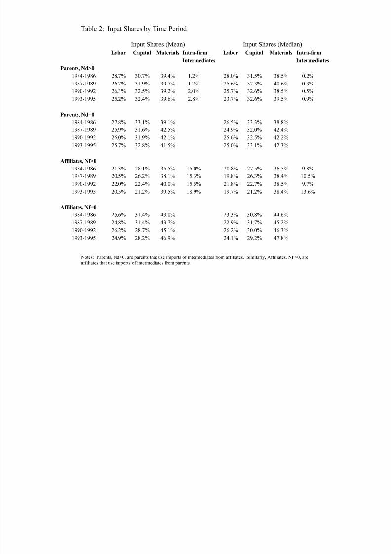
7/29/2019 MNC Related Doc
http://slidepdf.com/reader/full/mnc-related-doc 61/82
Table 2: Input Shares by Time Period
Notes: Parents, Nd>0, are parents that use imports of intermediates from affiliates. Similarly, Affiliates, NF>0, areaffiliates that use imports of intermediates from parents.
Input Shares (Mean) Input Shares (Median)
Labor Capital Materials Intra-firm Labor Capital Materials Intra-firm
Intermediates Intermediate
Parents, Nd>0
1984-1986 28.7% 30.7% 39.4% 1.2% 28.0% 31.5% 38.5% 0.2%1987-1989 26.7% 31.9% 39.7% 1.7% 25.6% 32.3% 40.6% 0.3%
1990-1992 26.3% 32.5% 39.2% 2.0% 25.7% 32.6% 38.5% 0.5%
1993-1995 25.2% 32.4% 39.6% 2.8% 23.7% 32.6% 39.5% 0.9%
Parents, Nd=0
1984-1986 27.8% 33.1% 39.1% 26.5% 33.3% 38.8%
1987-1989 25.9% 31.6% 42.5% 24.9% 32.0% 42.4%
1990-1992 26.0% 31.9% 42.1% 25.6% 32.5% 42.2%
1993-1995 25.7% 32.8% 41.5% 25.0% 33.1% 42.3%
Affiliates, Nf>0
1984-1986 21.3% 28.1% 35.5% 15.0% 20.8% 27.5% 36.5% 9.8%
1987-1989 20.5% 26.2% 38.1% 15.3% 19.8% 26.3% 38.4% 10.5%
1990-1992 22.0% 22.4% 40.0% 15.5% 21.8% 22.7% 38.5% 9.7%
1993-1995 20.5% 21.2% 39.5% 18.9% 19.7% 21.2% 38.4% 13.6%
Affiliates, Nf=0
1984-1986 25.6% 31.4% 43.0% 23.3% 30.8% 44.6%
1987-1989 24.8% 31.4% 43.7% 22.9% 31.7% 45.2%1990-1992 26.2% 28.7% 45.1% 26.2% 30.0% 46.3%
1993-1995 24.9% 28.2% 46.9% 24.1% 29.2% 47.8%

7/29/2019 MNC Related Doc
http://slidepdf.com/reader/full/mnc-related-doc 62/82
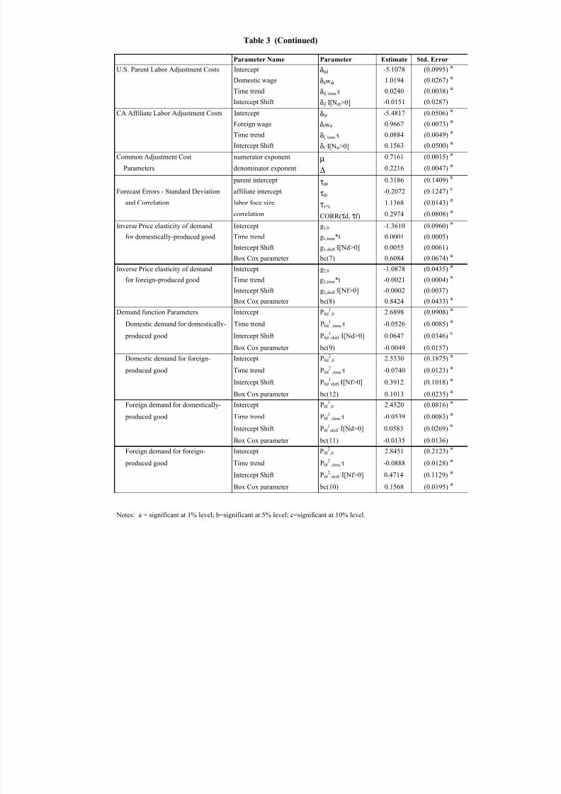
7/29/2019 MNC Related Doc
http://slidepdf.com/reader/full/mnc-related-doc 63/82
Table 3 (Continued)
Parameter Name Parameter Estimate Std. Error
U.S. Parent Labor Adjustment Costs Intercept δ0d -5.1078 (0.0995)a
Domestic wage δdwdt 1.0194 (0.0267)a
Time trend δd, time·t 0.0240 (0.0038)a
Intercept Shift δd·I[Ndt>0] -0.0151 (0.0287)
CA Affiliate Labor Adjustment Costs Intercept δ0f -5.4817 (0.0506)a
Foreign wage δf wft 0.9667 (0.0073)a
Time trend δf, time·t 0.0884 (0.0049)a
Intercept Shift δf ·I[Nft>0] 0.1563 (0.0500)a
Common Adjustment Cost numerator exponent µ 0.7161 (0.0015)a
Parameters denominator exponent ∆ 0.2216 (0.0047)a
parent intercept τd00.3186 (0.1409)
b
Forecast Errors - Standard Deviation affiliate intercept τf0-0.2072 (0.1247)
c
and Correlation labor foce size τ1*L1.1368 (0.0143)
a
correlation CORR(τd, τf) 0.2974 (0.0808)a
Inverse Price elasticity of demand Intercept g1,0 -1.3610 (0.0960)a
for domestically-produced good Time trend g1,time*t 0.0001 (0.0005)
Intercept Shift g1,shift·I[Nd>0] 0.0055 (0.0061)
Box Cox parameter bc(7) 0.6084 (0.0674)a
Inverse Price elasticity of demand Intercept g2,0 -1.0878 (0.0435)a
for foreign-produced good Time trend g2,time*t -0.0021 (0.0004)a
Intercept Shift g2,shift·I[Nf>0] -0.0002 (0.0037)
Box Cox parameter bc(8) 0.8424 (0.0433)a
Demand function Parameters Intercept P0d1,0 2.6898 (0.0908)
a
Domestic demand for domestically- Time trend P0d1 ,time·t -0.0526 (0.0085) a
produced good Intercept Shift P0d1shift·I[Nd>0] 0.0647 (0.0346)
c
Box Cox parameter bc(9) -0.0049 (0.0157)
Domestic demand for foreign- Intercept P0d2,0 2.5330 (0.1875)
a
produced good Time trend P0d2
,time·t -0.0740 (0.0123)a
Intercept Shift P0d2shift·I[Nf>0] 0.3912 (0.1018)
a
Box Cox parameter bc(12) 0.1013 (0.0235)a
Foreign demand for domestically- Intercept P0f 1,0 2.4520 (0.0816)
a
produced good Time trend P0f 1
,time·t -0.0539 (0.0083)a
Intercept Shift P0f 1shift·I[Nd>0] 0.0583 (0.0269)
b
Box Cox parameter bc(11) -0.0135 (0.0136)
Foreign demand for foreign- Intercept P0f 2,0 2.8451 (0.2123)
a
produced good Time trend P0f 2
,time·t -0.0888 (0.0128)a
Intercept Shift P0f 2,
shift·I[Nf>0] 0.4714 (0.1129)a
Box Cox parameter bc(10) 0.1568 (0.0195)a
Notes: a = significant at 1% level; b=significant at 5% level; c=significant at 10% level.

7/29/2019 MNC Related Doc
http://slidepdf.com/reader/full/mnc-related-doc 64/82
Table 4: Heterogeneous Logit Estimates for Trade Flows
Canadian Affiliate sales of Intermediates to U.S. parents
Parameter Name Symbol Estimate Std. Error
Exogenous covariates
Intercept
ψ 1o
-1.8682 (1.3094)
Domestic Capital share ψ 11αitKd 2.6540 (3.5285)
Foreign Capital share ψ 12αitKf -3.9909 (1.3219)
a
U.S. Tariff plus transportation cost at time t ψ 13(τdit +cdit) -3.5521 (9.4507)
Domestic Market power ψ 14g1it14.8839 (24.2639)
Domestic wages ψ 15wdit0.0025 (0.0155)
Foreign wages ψ 16wfit-0.0040 (0.0175)
Time trend ψ 17t -0.0640 (0.0404)
State Dependence
Indicator for positive flows at t-1 ψ 18I[Ndit-1>0] 2.7082 (0.2613) a
Initial conditions
Indicator for positive flows at t=1 ψ 19I[Ndi1>0] 2.0432 (0.3885)
a
U.S. Tariff plus transportation cost at time t=1 ψ 1,10(τdi1 +cdi ) 0.6535 (8.1493)
U.S. Parent Sales of Intermediates to Canadian Affiliates
Parameter Name Symbol Estimate Std. Error
Exogenous covariates
Intercept ψ 2o -1.2835 (1.6649)Foreign Capital share ψ 21αit
Kf -17.6723 (3.9726)a
Domestic Capital share ψ 22αitKd 5.3974 (2.9113)
c
Canadian Tariff plus transportation cost at time t ψ 23(τfit +cfit) -3.8424 (9.6310)
Foreign Market power ψ 24g2it62.1002 (19.1856)
a
Domestic wages ψ 25wdit0.0057 (0.0227)
Foreign wages ψ 26wfit-0.0276 (0.0264)
Time trend ψ 27t -0.0923 (0.0732)
State Dependence
Indicator for positive flows at t-1 ψ 28I[Nf it-1>0] 2.6841 (0.3699)
a
Initial conditions
Indicator for positive flows at t=1 ψ 29I[Nf i1>0] 3.1723 (0.6660)
a
Canadian Tariff plus transportation cost at time t=1 ψ 2,10(τfi1 +cfi1) -0.3242 (7.7293)
Notes: a = significant at 1% level; b=significant at 5% level; c=significant at 10% level.

7/29/2019 MNC Related Doc
http://slidepdf.com/reader/full/mnc-related-doc 65/82
Table 4: Heterogeneous Logit Estimates for Trade Flows (continued)
U.S. Parent Arms-Length Sales to Canada
Parameter Name Symbol Estimate Std. Error
Exogenous covariates
Intercept ψ 3o -2.3931 (1.5575)Domestic Capital share ψ 31αit
Kf 4.0199 (5.2116)
Canadian Tariff plus transportation cost at time t ψ 32(τfit +cfit) 6.7880 (9.7591)
Domestic Market power ψ 33g1it-33.2785 (25.1416)
Domestic wages ψ 34wdit0.0763 (0.0269)
a
Foreign wages ψ 35wfit-0.0295 (0.0323)
Time trend ψ 36t 0.0022 (0.0633)
State Dependence
Indicator for positive flows at t-1 ψ 37I[Eit-1>0] 2.9516 (0.4054)a
Initial conditionsIndicator for positive flows at t=1 ψ 38I[Ei1>0] 3.3328 (0.7916)
a
Canadian Tariff plus transportation cost at time t=1 ψ 39(τfi1 +cfi1) -7.6606 (7.8508)
Canadian Affiliate Arms-Length Sales to the U.S.
Parameter Name Symbol Estimate Std. Error
Exogenous covariates
Intercept ψ 4o-0.3746 (0.7916)
Foreign Capital share ψ 41αitKf 2.6306 (1.9747)
U.S. Tariff plus transportation cost at time t
ψ 42(τdit +cdit)-0.0552 (9.9939)
Foreign Market power ψ 43g1it-30.3235 (10.8977)
a
Domestic wages ψ 44wdit-0.0165 (0.0162)
Foreign wages ψ 45wfit-0.0018 (0.0156)
Time trend ψ 46t -0.0430 (0.0364)
State Dependence
Indicator for positive flows at t-1 ψ 47I[Iit-1>0] 2.5033 (0.2408)a
Initial conditions
Indicator for positive flows at t=1 ψ 48I[Ii1>0] 2.0843 (0.3913)a
U.S. Tariff plus transportation cost at time t=1 ψ 49(τdi1 +cdi1) -12.0584 (8.9857)
Covariance Matrix: Logit Random Effects
µ ND µ NF µE µI
µ ND 1.8843a
µ NF 1.9975a 2.9511 b
µE 1.0310 b 1.0927 b 3.1797 b
µI 1.4941a 1.0196 b 0.9690c 2.2521a
Notes: a = significant at 1% level; b=significant at 5% level; c=significant at 10% level.

7/29/2019 MNC Related Doc
http://slidepdf.com/reader/full/mnc-related-doc 66/82
Table 5: Simulated Responses to Tariff Changes
Notes: Trade flows are expressed in thousands 1984 dollars. The table reports mean valuesover firms with a positive value for the indicated flow.
U.S. Canadian U.S. Parent U.S. Parent Canadian
Parent affiliate intermediates Arms-Length affiliate sales in sales in sales to sales to intermediates Ar
the U.S. Canada to Canadian Canada sales to
affiliates U.S. Parents
Pd1Sd Pf
2Sf Pd
1 Nf Pf
1E Pf
2 Nd
1995 Baseline Simulation Steady State Level 3619683 213074 241630 37700 325587
Experiment: Fixed tariffs at 1984 level 3588695 198422 229852 30116 317977
% difference from Base -0.9% -6.9% -3.9% -19.0% -2.2%
Experiment: Eliminate tariffs 3640632 226825 253316 48014 330548
% difference from Base 0.6% 6.5% 6.6% 28.4% 2.1%
% difference from Tariffs=1984 1.4% 14.3% 11.0% 58.5% 4.4%

7/29/2019 MNC Related Doc
http://slidepdf.com/reader/full/mnc-related-doc 67/82
Table 6: Percentage Changes 1984-1995: Data and Model Predictions
Model Decomposition
Data Model Tariffs Technology Wages Other
USP Sales
Domestic (Pd1Sd) -19.6 -9.0 0.8 4.0 -4.3 -9.5
Intra-firm (Pd1 Nf ) 73.3 99.1 9.7 71.8 14.4 3.2Arms-Length (Pf
1E) 75.3 79.1 36.0 9.0 -1.3 35.4
Total -17.1 -6.0 1.1 7.3 -3.9 -10.5
Total Net -20.2 -9.8 1.0 3.8 -3.9 -10.7
CA Sales
Domestic (Pf 2Sf ) -17.9 -6.9 6.4 -71.9 18.3 40.3
Intra-firm (Pf 2 Nd) 94.5 123 5.2 84.1 -2.9 36.6
Arms-Length (Pd2I) 4.0 8.9 32.5 37.9 -20.5 -41.0
Total 18.7 38.3 7.3 7.8 11.2 12.0Total Net -0.5 14.2 6.3 -23.3 9.9 21.3
MNC Sales -19.0 -8.4 1.3 2.4 -3.0 -9.1
USP Employment -24.4 -12.6 1.4 12.4 -1.6 -24.8
CA Employment -14.1 -3.0 9.0 15.5 -7.0 -20.5
Notes: "Data" shows percentage change in our analysis data set. "Model" shows percentage change from 1984-95
in the model simulation. Under "Model Decomposition," we compare the % change predicted by the model under the baseline simulation, with the % change the model predicts under the counterfactual that the indicated forcingvariable (tariffs, technology or wages) stayed fixed at the 1984 level. The difference is the percentage changeattributable to changes in that particular forcing variable.

7/29/2019 MNC Related Doc
http://slidepdf.com/reader/full/mnc-related-doc 68/82
A1
Appendix 1: The Mapping from the Data to the Stochastic Terms of the Model
The mapping from the data to the stochastic terms of the model is obtained by solving thesystem of nonlinear equations given by the FOCs and the production functions. If the MNCutilizes all four trade flows (bilateral intra-firm and arms length flows) this is a system of 12
equations in 12 unknowns. We describe the solution in this general case.
Step 1: By summing the FOCs for Ld , K d , M d and N d (see eqn. (19) in Section IV.2) we obtain:
(A1.1) 0 L ) FD( E B ) N P ( g CD )Q P )( A g 1( d d d 2
f 2d 1
d 1 =δ−+−−
Similarly, for the affiliate, we obtain:
(A1.2) 0 L ) FF ( E A ) N P ( g CF )Q P )( B g 1( f f f 1
d 1 f 2
f 2 =δ−+−−
where CD and CF are U.S. and Canadian costs, respectively (including capital, labor, materialsand intermediates, but not adjustment costs). We have utilized the CRTS assumption to eliminate
the share parameters, leaving g 1 and g 2 as the only unknown parameters in (A1.1) and (A1.2).However, the variables d
1d Q P and f
2 f Q P are not observed, so we cannot yet solve for g 1 and g 2.
Step 2: We can express d 1
d Q P and f 2
f Q P in terms of observed data as follows:
(A1.3) ) E P ( ) P P ( N P S P Q P 1 f
1 f
1d f
1d d
1d d
1d
++=
(A1.4) ) I P ( ) P P ( N P S P Q P 1d
2d
2 f d
2 f f
2 f f
2 f
++=
Here, only the price ratios P d 1 /P f
1and P f
2 /P d
2are not observed. At this point, it is convenient to
denote these price ratios as PR1 and PR2, and treat them as unknown parameters.Before proceeding, it is useful to give an intuition for identification of g 1 and g 2. First,
consider what (A1.1) and (A2.1) imply in the special case of no intra-firm intermediates. In thatcase, the g 2(P f
2 N d )B and g 1(P d
1 N f )A terms drop out, so we can consider each equation separately.
Furthermore, A=B=1, and, as we discussed in section IV.2, the domestic to foreign price ratios
depend only on the wedge created by tariff and transport costs. Therefore, d 1
d Q P and f 2
f Q P are
observable, and they are exactly equal to total revenues (net of tariff and transport costs) of the
parent and affiliate. Denote these by RD and RF .40 Then we get g 1 = (RD-CD- δ d E(FD)Ld )/RD,which is the usual Lerner markup equation in the CRTS case, modified to account for expectedlabor force adjustment costs. Thus, g 1 and g 2 are basically identified from price/cost markups.
With, intra-firm trade in intermediates, the price ratios PR1 and PR2 are not observed, wehave 0<A<1 and 0<B<1, and the g 2(P f
2 N d )B and g 1(P d
1 N f )A terms matter, so (A1.1) and (A1.2)
must be solved jointly. All three of these changes reflect the fact that with intra-firm trade inintermediates, the firm’s incentive to hold down output to increase prices is mitigated becausehigher output prices also imply higher tariff and transport costs.
Fortunately, the price ratios PR1 and PR2 depend only on tariff and transport costs and on g 1 and g 2. For instance, the FOC for E shows how the parent’s incentive to hold down P d
1to
avoid tariff and transport costs on shipping N f to the Canadian affiliate depends on g 1, tariffs and
40 Note that RD=P d 1S d + P d
1 N f + (1-T f -C f )(P f 1 E). In the absence of intra-firm trade in intermediates, P f
1 / P d 1 = 1/(1-
T f -C f ), so the last term reduces to P d 1 E , the value of exports at domestic prices. Hence, P d
1Qd = RD.
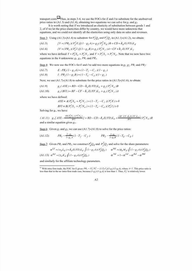
7/29/2019 MNC Related Doc
http://slidepdf.com/reader/full/mnc-related-doc 69/82
A2
transport costs.41 Thus, in steps 3-4, we use the FOCs for E and I to substitute for the unobserved price ratios in (A1.3) and (A1.4), obtaining two equations we can solve for g 1 and g 2.
It is worth noting that if we introduced an elasticity of substitution between goods 1 and2, of if we let the price elasticities differ by country, we would have more unknowns thatequations, and we could not identify all the elasticities using only data on sales and revenues.
Step 3: Using (A1.3)-(A1.4) to substitute for d 1
d Q P and f 2
f Q P in (A1.1)-(A1.2), we obtain:
(A1.5) d d d 2
f 211
f 1 L ) FD( E CD B ) N P ( g ) A g 1 )]( E P )( PR( Y [ δ +=+−+
(A1.6) f f f 1
d 121
d 2 L ) FF ( E CF A ) N P ( g ) B g 1 )]( I P )( PR( V [ δ+=+−+
where we have defined f 1
d d 1
d N P S P Y += and d 2
f f 2
f N P S P V += . Note that we now have two
equations in the 4 unknowns: g 1, g 2, PR1 and PR2.
Step 4: We now use the FOCs for E and I to add two more equations in g 1, g 2, PR1 and PR2:
(A1.7) ) g 1 )( C T 1( ) A g 1( PR: E 1 f f 11 −−−=−
(A1.8) ) g 1 )( C T 1( ) B g 1( PR: I 2d d 22 −−−=−
Next, we use (A1.7)-(A1.8) to substitute for the price ratios in (A1.5)-(A1.6), to obtain:
(A1.9) B ) N P ( g L ) FD( E CD RD ) AYE ( g d 2
f 2d d 1 +δ−−=
(A1.10) A ) N P ( g L ) FF ( E CF RF ) BVI ( g f 1
d 1 f f 2 +δ−−=
where we have defined:
0 ) E P )( C T 1( ) N P S P ( A AYE 1
f f f f 1
d d 1
d >−−++≡
0 ) I P )( C T 1( ) N P S P ( B BVI 2
d d d d 2
f f 2
f >−−++≡
Solving for g1, we have:
B ) N P ( L ) FD( E CD RD ] AYE [ g )11.1 A( d 2
f BVI
) L ) FF ( E CF RF (
d d BVI
) N P )( N P ( AB
1 f f d
2 f f
1d δ
δ −−
+−−=−
and a similar equation gives g 2.
Step 6: Given g 1 and g 2, we can use (A1.7)-(A1.8) to solve for the price ratios:
(A1.12) )C T 1( PR f f A g 1
g 11
1
1 −−=−−
)C T 1( PR d d B g 1
g 12
2
2 −−= −−
Step 7: Given PR1 and PR2, we construct d d Q P 1 and f f
Q P 2 and solve for the share parameters:
)Q P )( A g 1( L ) FD( E ) Lw( d 1d 1d d d d
Ld −+= δ α )Q P )( A g 1( ) M ( d 1d 1d d
Md −= φ α
(A1.13) )Q P )( A g 1( ) K ( d 1d 1d d
Kd −= γ α Md Kd Ld Nd α α α α −−−= 1
and similarly for the affiliate technology parameters.
41 With intra firm trade, the FOC for E gives: PR1 = P d 1 /P f
1 = (1-T f -C f )(1-g 1 )/(1-g 1 A), where A<1. This price ratio isless than that in the no intra-firm trade case, because (1-g 1 )/(1-g 1 A) is less than 1. Thus, P d
1 is relatively lower.
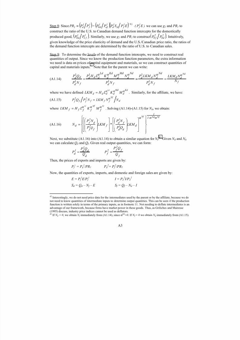
7/29/2019 MNC Related Doc
http://slidepdf.com/reader/full/mnc-related-doc 70/82
A3
Step 8: Since ( ) ( )( ) ) E P ( E P S P P P P P PR 1 f
1 f d
1d
1of
1d 0
1 f
1d 1
1 g ⋅
−=≡ we can use g 1 and PR1 to
construct the ratio of the U.S. to Canadian demand function intercepts for the domestically
produced good, )1 f 0
1d 0 P P . Similarly, we use g 2 and PR2 to construct )2
d 02 f 0 P P . Intuitively,
given knowledge of the price elasticity of demand and the U.S./Canadian price ratio, the ratios of
the demand function intercepts are determined by the ratio of U.S. to Canadian sales.
Step 9: To determine the levels of the demand function intercepts, we need to construct realquantities of output. Since we know the production function parameters, the extra informationwe need is data on prices of ca pital equipment and materials, so we can construct quantities of capital and materials inputs.42 Note that for the parent we can write:
(A1.14) f
d d
f d
Nd
d d d
f d
Nd
d
Md
d
Kd
d
Ld
d d d
f d
d d N
N LKM
N P
N LKM P
N P
N M K L H P
N P
Q P Nd α α α α α α
=≡=1
1
1
1
1
1
where we have defined Kd Md
d d d d d M K L H LKM Ld
α α α = . Similarly, for the affiliate, we have:
(A1.15) d f f f 2
f f 2
f N N LKM N P Q P
Nf α =
where Kf M Lf
f f f f f M K L H LKM f α α α = . Solving (A1.14)-(A1.15) for N d , we obtain:
(A1.16)
Nf Nd Nf 11
d
d 1d
f 1d
f
f Q2
f
d 2
f d LKM
Q P
N P * LKM
P
N P N
α α α −
=
Next, we substitute (A1.16) into (A1.14) to obtain a similar equation for N f .43 Given N d and N f ,we can calculate Qd and Q f . Given real output quantities, we can form:
d
d 1d 1
d Q
Q P P =
f
f 2
f 2 f Q
Q P P =
Then, the prices of exports and imports are given by:
P f 1
= P d 1 /PR1 P d
2= P f
2 /PR2
Now, the quantities of exports, imports, and domestic and foreign sales are given by:
E = P f 1 E/P f
1 I = P d 2 I/P d
2
S d = Qd – N f – E S f = Q f – N d – I
42 Interestingly, we do not need price data for the intermediates used by the parent or by the affiliate, because we donot need to know quantities of intermediate inputs to determine output quantities. This can be seen if the productionfunction is written solely in terms of the primary inputs, as in footnote 11. Not needing to deflate intermediates is anadvantage of our framework, because firms have market power in these goods. Thus, as Griliches and Mairesse(1995) discuss, industry price indices cannot be used as deflators.43 If N d = 0, we obtain N f immediately from (A1.14), since α Nd =0. If N f = 0 we obtain N d immediately from (A1.15).

7/29/2019 MNC Related Doc
http://slidepdf.com/reader/full/mnc-related-doc 71/82
A4
Finally, we can write the demand function intercepts as:
2
2
g 2d
2d 0
g f
2 f
2 f 0
I P P
S P P
=
=
1 g 1 f
1 f 0
g d
1d
1d 0
E P P
S P P 1
=
=
In the case that I=0,
2
d P and
2
d 0 P will be undefined, but
2
f 0 P can still be calculated since
d f f N QS −= . In the case that E=0, 1 f P and 1
f 0 P will be undefined, but 1d 0 P can still be calculated
since f d d N QS −= .
Step 10: Once we have solved for the 12 firm specific technology and demand parameters, it is
straightforward to map these into the ε vector using the equations of the stochastic specificationdescribed in section III.3.
Appendix 2: Identification of H, P0 and R
As discussed in Appendix 1, the sources of identification for the Cobb-Douglas share
parameters, price elasticities of demand, and demand function intercept ratios are rather obviousin the context of our model. This is also true of the labor force adjustment cost parameters, whichare pinned down by the persistence of employment over time. Much more subtle, however, is thesource of identification of the H , P 0 and R parameters, which are TFP, the demand interceptlevels, and the profit rate. Here we give the intuition for how these parameters are identified.
Regarding TFP, recall that we normalize H t =1 and t=0 in 1983, and specify that TFPgrowth is determined by H t = (1+h)
t , where h is an estimated parameter. It is not immediately
obvious is how growth in H would be separately identified from changes in the demand functionintercepts P 0 if output prices and quantities are not separately observed. One might think that,since any observed revenue level can be explained by a locus of price and quantity values, itwould be impossible to disentangle H and the P 0. However, this is not the case.
Consider a simple autarky case (a single firm with no affiliate), and with K and L as theonly inputs, and no adjustment costs. Then we have:
L K
L K H Q α α ⋅= g 0Q P P
−= wL K PQ −−= γ Π
In this case, labor demand is:
g 1
g 1
L
K ) g 1(
0
L K
w H P ) g 1(
w L
−
=
−
−α
α γ
α α
Calculating elasticities of labor demand with respect to H and P 0, we obtain:
(A2.1) 0 g
1
P
L
L
P
0
0 >=∂∂ 0)1(1 >−=
∂∂ g
g H
L
L
H
Thus, both TFP growth and growth in demand ( P 0) cause growth of the firm. If all growth is dueto growth in demand, then a firm’s growth rate will be inversely proportional to its g . But if allgrowth is due to TFP growth, then firm growth rates will decline even more quickly with g .Thus, to the extent that firm employment growth is less than proportional to 1/g (i.e., it is muchslower among high g firms), we will conclude that TFP is a bigger factor in growth than P 0.
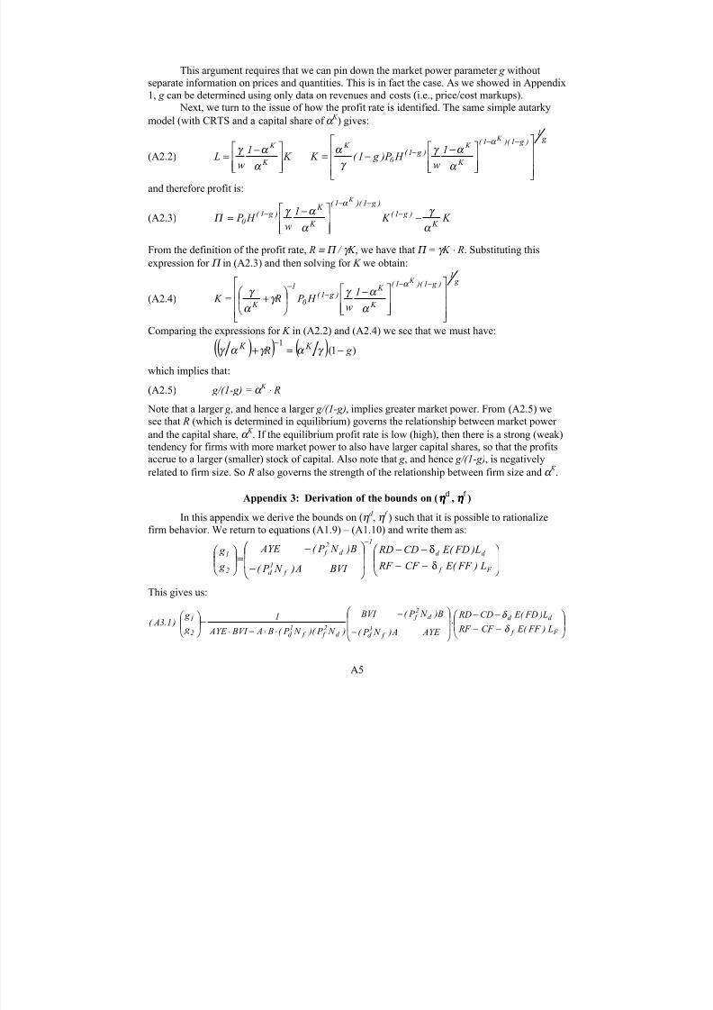
7/29/2019 MNC Related Doc
http://slidepdf.com/reader/full/mnc-related-doc 72/82
A5
This argument requires that we can pin down the market power parameter g withoutseparate information on prices and quantities. This is in fact the case. As we showed in Appendix1, g can be determined using only data on revenues and costs (i.e., price/cost markups).
Next, we turn to the issue of how the profit rate is identified. The same simple autarky
model (with CRTS and a capital share of α K ) gives:
(A2.2) K 1
w L
K
K
−=
α
α γ
g 1 ) g 1 )( 1(
K
K ) g 1(
0
K K
1
w H P ) g 1( K
−−=
−−−
α
α
α γ
γ
α
and therefore profit is:
(A2.3) K K 1
w H P
K
) g 1(
) g 1 )( 1(
K
K ) g 1(
0
K
α
γ
α
α γ Π
α
−
−= −
−−−
From the definition of the profit rate, R ≡ Π / γ K , we have that Π = γ K ⋅ R. Substituting this
expression for Π in (A2.3) and then solving for K we obtain:
(A2.4)
g 1
) g 1 )( 1(
K
K ) g 1(
0
1
K
K
1
w H P R K
−
+=−−
−− α
α
α γ γ
α
γ
Comparing the expressions for K in (A2.2) and (A2.4) we see that we must have:
( )( ) ( ) )1(1
g R K K −=+
−γ α γ α γ
which implies that:
(A2.5) g/(1-g) = α K ⋅ R
Note that a larger g , and hence a larger g/(1-g), implies greater market power. From (A2.5) wesee that R (which is determined in equilibrium) governs the relationship between market power
and the capital share, α K . If the equilibrium profit rate is low (high), then there is a strong (weak)
tendency for firms with more market power to also have larger capital shares, so that the profitsaccrue to a larger (smaller) stock of capital. Also note that g , and hence g/(1-g), is negatively
related to firm size. So R also governs the strength of the relationship between firm size and α K .
Appendix 3: Derivation of the bounds on (ηηηηd, ηηηηf
)
In this appendix we derive the bounds on (ηd , η f ) such that it is possible to rationalizefirm behavior. We return to equations (A1.9) – (A1.10) and write them as:
δ−−δ−−
−
−=
−
F f
d d
1
f 1
d
d 2
f
2
1
L ) FF ( E CF RF
L ) FD( E CD RD
BVI A ) N P (
B ) N P ( AYE
g
g
This gives us:
−−−−
⋅
−
−
⋅⋅−⋅=
F f
d d
f 1d
d 2
f
d 2
f f 1d 2
1
L ) FF ( E CF RF
L ) FD( E CD RD
AYE A ) N P (
B ) N P ( BVI
) N P )( N P ( B A BVI AYE
1
g
g )1.3 A(
δ
δ
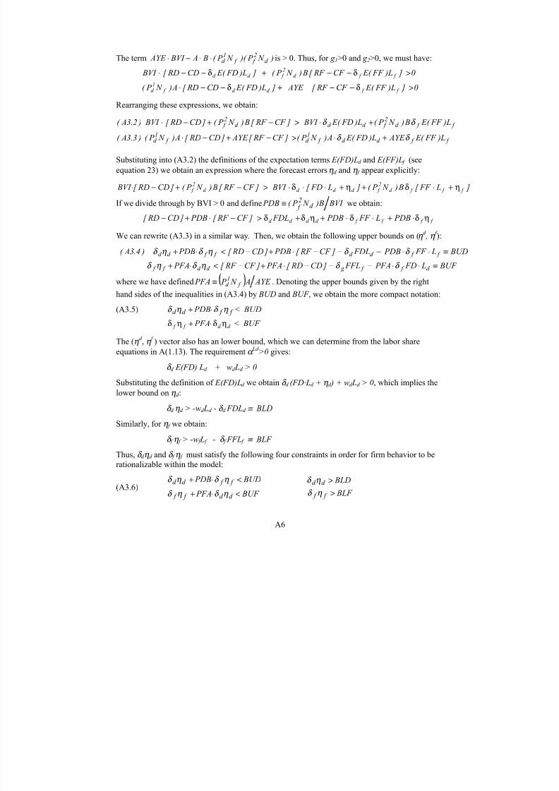
7/29/2019 MNC Related Doc
http://slidepdf.com/reader/full/mnc-related-doc 73/82
A6
The term ) N P )( N P ( B A BVI AYE d 2
f f 1d ⋅⋅−⋅ is > 0. Thus, for g 1>0 and g 2>0, we must have:
0 ] L ) FF ( E CF RF [ B ) N P ( ] L ) FD( E CD RD[ BVI f f d 2
f d d >δ−−+δ−−⋅
0 ] L ) FF ( E CF RF [ AYE ] L ) FD( E CD RD[ A ) N P ( f f d d f 1
d >δ−−+δ−−⋅
Rearranging these expressions, we obtain:
f f d 2
f d d d 2
f L ) FF ( E B ) N P ( L ) FD( E BVI ]CF RF [ B ) N P ( ]CD RD[ BVI )2.3 A( δ δ +⋅>−+−⋅
f f d d f 1d f
1d L ) FF ( E AYE L ) FD( E A ) N P ( ]CF RF [ AYE ]CD RD[ A ) N P ( )3.3 A( δ δ +⋅>−+−⋅
Substituting into (A3.2) the definitions of the expectation terms E(FD)Ld and E(FF)L f (see
equation 23) we obtain an expression where the forecast errors ηd and η f appear explicitly:
] L FF [ B ) N P ( ] L FD[ BVI ]CF RF [ B ) N P ( ]CD RD[ BVI f f f d 2
f d d d d 2
f η+⋅δ+η+⋅⋅δ⋅>−+−⋅
If we divide through by BVI > 0 and define BVI B ) N P ( PDB d 2
f ≡ we obtain:
f f f f d d d d PDB L FF PDB FDL ]CF RF [ PDB ]CD RD[ ηδ⋅+⋅δ⋅+ηδ+δ>−⋅+−
We can rewrite (A3.3) in a similar way. Then, we obtain the following upper bounds on (ηd , η f ):
BUF L FD PFA FFL ]CD RD[ PFA ]CF RF [ PFA
BUD L FF PDB FDL ]CF RF [ PDB ]CD RD[ PDB )4.3 A(
d f f g d d f f
f f d d f f d d
≡⋅⋅−−−⋅+−<⋅+
≡⋅⋅−−−⋅+−<⋅+
δ δ ηδ ηδ
δ δ ηδ ηδ
where we have defined ) AYE A N P PFA f 1d ≡ . Denoting the upper bounds given by the right
hand sides of the inequalities in (A3.4) by BUD and BUF , we obtain the more compact notation:
(A3.5) f f d d PDB ηδ ηδ ⋅+ < BUD
d d f f PFA ηδ⋅+ηδ < BUF
The (ηd , η f ) vector also has an lower bound, which we can determine from the labor share
equations in A(1.13). The requirement α Ld >0 gives:
δ d E(FD) Ld + wd Ld > 0
Substituting the definition of E(FD)Ld we obtain δ d (FD·Ld + ηd ) + wd Ld > 0, which implies the
lower bound on ηd :
δ d ηd > -wd Ld - δ d FDLd ≡ BLD
Similarly, for η f we obtain:δ f η f > -w f L f - δ f FFL f ≡ BLF
Thus, δ d ηd and δ f η f must satisfy the following four constraints in order for firm behavior to berationalizable within the model:
(A3.6) BUF PFA
BUD PDB
d d f f
f f d d
<⋅+
<⋅+
ηδ ηδ
ηδ ηδ
BLF
BLD
f f
d d
>>
ηδ
ηδ
7/29/2019 MNC Related Doc
http://slidepdf.com/reader/full/mnc-related-doc 74/82
A7
Note that the upper bound for δ d ηd depends on δ f η f , and vice-versa. We can write an
unconditional upper bound for δ d ηd in terms of BLF , the lower bound for δ f η f , as follows:
δ d ηd + (PDB) (BLF) < BUD
This equation defines the largest possible δ d ηd such that firm behavior can be rationalized by
some value of η f . If δ d ηd is larger than [BUD – (PDB) · (BLF)] then it is impossible to find a δ f η f small enough so that the first equation in (A3.6) is satisfied. So the feasible range for δ d ηd is:
BLD < δ d ηd < BUD – (PDB)(BLF).
This translates into an (unconditional) feasible range for ηd of:
d
d
d
) BLF )( PDB( BUD BLD
δ−
<η<δ
or, substituting in the definitions of BLD, BUD, BLF and PDB we have:
(A3.7)d d
f f
d d d
d d L FD Lw PDB ]CF RF [ PDB ]CD RD[
L FD Lw
⋅−δ
⋅+−⋅+−<η<⋅−
δ−
We rewrite (A3.7) more compactly as:
(A3.9) BLd
< ηd < BU d
Now, suppose we have drawn a value of ηd that satisfies (A3.9), and denote this value by
ηd,m where m indicates the draw. Then the conditional bounds on η f are determined as follows:
Substituting ηd,m into (A3.3) we have:
] L FF [ AYE
] L FD[ A ) N P ( ]CF RF [ AYE ]CD RD[ A ) N P (
f f f
m ,d d d f 1d f
1d
ηδ
ηδ
+⋅⋅+
+⋅⋅>−⋅+−⋅
which implies that:
)] L FD( CD RD[ AYE
A ) N P ( L FF
CF RF m ,d d d
f 1
f f
f f ηδ
δ η +⋅⋅−−⋅+⋅−
−<
Thus, draw m for η f must satisfy this upper bound. We write this more compactly as:
(A3.10) )m( f m
f BU <η
Recall we have already derived δ f η f > BLF , which we can write as η f > BLF/ δ f ≡ BL f .Combining this with (A3.9) and (A3.10) we have the following bounds for sequential draws of
ηd and η f :
(A3.11)
<η<
<η<
)m( f m
f f
d d
d
BU BL
BU BL⇒ η ∈ Β D
The recursive simulation algorithm described in Appendix 4 will work by first drawing a value
for ηd from its truncated distribution given the first set of unconditional bounds in (A3.11), and
then drawing a value for η f from the second set of conditional bounds in (A3.11). Of course,draws obtained in this sequential fashion will not have the correct joint distribution. The draws

7/29/2019 MNC Related Doc
http://slidepdf.com/reader/full/mnc-related-doc 75/82
A8
so obtained must be weighted using an importance sampling algorithm in order to obtainsimulation consistent estimates of likelihood contributions. Appendix 4 derives the weights.
Appendix 4: Algorithm for Implementing the Smooth Recursive Simulator
In this appendix we present the recursive importance sampling algorithm for simulating
the likelihood contribution of a firm. Since the firm’s choice variables are continuous, but thestochastic terms must satisfy certain bounds in order for firm behavior to be rationalizable (seeAppendix 3), this algorithm is a discrete/continuous analogue of the GHK method.
Consider first the simulation for firm i in period t . We define ηt ≡ ( ηd t , η f
t ). From
(A3.11), the constraints on ηt are (suppressing firm subscripts):d t dt
d t BU BL <<η )( BU BL
dt f t ft
f t ηη <<
Let:
=
* ft ft
*dt dt
ft
dt
ησ
ησ
η
η
where σ dt and σ ft are the standard deviations of ηdt and η ft , and *dt η and *
ft η are standard normal.
We allow the forecast errors to be correlated across the parent and affiliate within a period.
Given the structure of the model, any shock that affects Ld,t+1 would also potentially affect
L f,t+1. Then, employing a lower triangular Cholesky decomposition, we have:
=
f
d
ft
dt
aa ζ
ζ
η
η
2212*
*01
where dζ and f ζ are iid N(0,1) and .1222
212 =+ aa Let F( ⋅ ) denote the standard normal distribution
function. The simulation algorithm proceeds as follows:
Step 1: Calculate
σdt
d t BL
F and
σdt
d t BU
F
Step 2: Draw a uniform random variable on [0,1]. Denote it by mt 1u .
Step 3: Construct
σ−
σ⋅+
σ=
dt
d t
dt
d t m
t 1
dt
d t *
1
BL F
BU F u
BL F u
Step 4: Construct )u( F *1
1md
−=ζ and md dt
mdt
ζ σ η =
Step 5: Calculate the bounds on f ζ , given md
ζ . These are:
)(2212 mdt f t f md ft f t BU aa BL ηζ ζ σ <+<
Or, rearranging terms:
ζ−
σ<ζ<
ζ−
σmd 12
ft
f t
22
f md 12
ft
f t
22
a BU
a
1a
BL
a
1

7/29/2019 MNC Related Doc
http://slidepdf.com/reader/full/mnc-related-doc 76/82

7/29/2019 MNC Related Doc
http://slidepdf.com/reader/full/mnc-related-doc 77/82
A10
conditional on data in the general class of continuous nonlinear models where this distribution isnot degenerate (e.g., random effects models, mixture models, factor models).
To describe the algorithm, it is useful to first explain implementation for a single time period (ignoring the panel aspect of the data). First we establish some definitions. Let D denotethe vector of data elements for a particular firm, and let S denote the vector of stochastic terms
for this firm (in our case D is 12x1 and S = (ε , η) where ε is 12x1 and η is 2x1, so S is 14x1). Let M denote the mapping from S to D: D=M(S). Note that M is not invertible, because thedimension of S exceeds that of D. Let B(D) denote the set of S values that are consistent with D:
B(D) = { S | D = M(S) }
If we partition S into sub-vectors S = (S 1 , S
2 ), then we can also define sets of values for the sub-
vectors that are consistent with D:
B1(D) = { S
1| D = M(S
1 ,S
2 ) for some S
2 } = { S
1| ∃ S
2such that D=M(S
1 ,S
2 )}
We can construct these sets recursively:
B2
(D | S 1
) = { S 2
| D = M(S 1
, S 2
) }Use P(X) to denote the measure of a set X and note that P(B(D))=0 under the unconditionaldistribution of S . The fact that P(B(D))=0 means that not only is A/R sampling impractical, it isimpossible in this case. A recursive algorithm is essential.
Since D = M(S) we have f( S , D ) = f(S) and:
f(S | D) = ) D( BS if 0
) D( BS if f(S)/f(D)
∉∈
Observe that:
[ ]∫ =∈ )(
)()( D BS
S d D f S f 1)()()(
1 ∫ =∈
−
D BS
S d S f D f
Thus, we have that f(S | D) ∝ f(S) if S ∈ B(D). But this is not immediately useful, because we
cannot draw directly from f(S) subject to the constraint that S ∈ B(D), since P(B(D)) = 0.Feasible methods to obtain draws from B(D) will generally involve drawing from an
incorrect “source” density φ (S) chosen so that P φ (B(D)) > 0, or ideally, P φ (B(D)) = 1, and φ (S)
>0 for all S ∈ B(D) subject to f(S) > 0. Thus, the general problem is to simulate draws from the
target density f(S | D) given that we only have access to draws from the source density φ (S) .The solution is an importance sampling algorithm in which the draws {S m }m=1, M from
φ (S) are weighted using weights wm such that wm ∝ f(S m )/ φ (S m ) for S m∈ B(D) and wm = 0 otherwise. Since weights must sum to 1, we have:
wm =otherwise 0
B(D)S if )(S )/ Kf(S mmm ∈φ where ∑=
∈=
M
) D( BS .t . s1m
mm
m
)S ( )S ( f K φ .
Maximal efficiency of an importance sampling algorithm is achieved by choosing a φ (S) as
“close” as possible to f(S | D), e.g., using Kullback–Liebler distance. Note that if φ (S) is veryclose to f(S | D), then the wm will be close to 1/M .
We now describe the application of this algorithm to our model. Consider a single periodof data for a firm. The data vector D is 12x1. The vector of stochastic terms S is 14x1. It consists

7/29/2019 MNC Related Doc
http://slidepdf.com/reader/full/mnc-related-doc 78/82
A11
of ε which is 12x1, and η which is 2x1. We have that D = M( ε , η ) and consider a partition:
B(D) = { ( ε , η ) | D = M( ε , η ) } B
1(D) = { η | ∃ ε s.t. D = M( ε , η ) }
B2(D | η ) = { ε | D= M( ε , η ) }
Given our model and distributional assumptions, we have seen that P(B(D)) = 0, 0<P(B1
(D))<1,and P(B
2(D| η ))=0. It is not feasible to draw directly from the joint distribution f( ε , η | D).
Rather, we draw sequentially, first obtaining ηm ∈ B1(D) and then constructing the implied ε m
using the relation D= M( ε m , ηm ), which is given by the nonlinear system of equations describedin Appendix 1. Thus, we use the source density:
φ (ε , η) =otherwise0
) D( Bif ) g( 1∈ηη
where g( η ) is the density from which we draw the ηm.
We emphasize that g(η) is not the “correct” density of η, given by f( η |η∈ B1(D)).
Rather, g( η ) is the density induced by the procedure of drawing η using the recursive importance
sampling algorithm discussed in Appendices 4. Recall that we draw η =(ηd , η f ) sequentially,rather than drawing directly from the correct joint density f (ηd , η f
| η ∈ B1(D)). Thus, we
sequentially partition the set B1(D) as follows:
B1d
(D) = { ηd | ∃ η f s.t. ( ηd
, η f ) ∈ B
1(D) }
B1f
(D, ηd ) = { η f | ( η
d , η f
) ∈ B1(D) }
We first draw ηd ∈ B
1d (D) and then, conditional on the draw ηd,m, we draw η f,m ∈ B
1f (D, ηd,m ).
Given this procedure, we have that g(η) is given by:
)())((/)()(
)()(
)(
)()(
)(),( ),(
11
),(1)(1
d m D
f d f m
d m
d m D f B f
f f
f m
Dd Bd
d d
d m f
md m B P D B P f f
d f
f
d f
f g ηηη
ηη
η
ηη
ηηη
ηηη
=
∫ ∫
=
∈∈
Thus we have that our source density is:
φ ( ε m , ηm ) =otherwise0
) D( Bif ) B( P ) B( P )( f )( f 1m
d m
f 1d 1 f m
d m ) , D( ) D( ∈ηηηη
Therefore, the importance sampling weights wm = f (ε m, ηm )/ φ ( ε m , ηm ) are:
wm =otherwise0
) D( B ) ,( if ) B( P ) B( P )( f K 1mm
d m
f 1d 1m ) , D( ) D( ∈ε ηηε
where:1 M
1m
)d m , D(
f 1 ) D(
d 1m ) B( P ) B( P )( f K
−
=
= ∑ ηε
Since we have chosen the source density φ (·) so that all draws (ε m, ηm) ∈ B(D), and since P(B
1d (D) ) appears in the numerator and denominator of wm , we can simplify to:
∑==
M
1m
d m
f 1d m
f 1mm ) B( P ) B( P )( f w ) , D( ) , D( ηηε .
7/29/2019 MNC Related Doc
http://slidepdf.com/reader/full/mnc-related-doc 79/82
A12
The sequential construction of the importance sampling weight for draw sequence m is exactlyanalogous to the construction of sequence weights in the GHK algorithm. The sequence that
begins with d mη is given more (less) weight to the extent that d
mη makes a valid draw for η f more
(less) likely. And a sequence that begins with ),( f m
d m ηη is given more (less) weight if the implied
ε m is more (less) likely. In fact, the algorithm described here is the continuous data analogue tothe algorithm for constructing and weighting draw sequences that underlies the GHK algorithm.
Given the recursive structure of the sequence weights, extension to the multi-period caseis obvious – but notationally burdensome – so we omit the specific expressions.
Appendix 6: The Firm’s Decisions to Engage in Imports, Exports, and Intra-Firm Trade
Finally, we turn to the problem that not all firms utilize all four trade flows ( N d , N
f , E, I )
in each period. We specify reduced form approximations to the firm’s decision rule regarding N
d >0, N f >0, E >0 and I >0 and estimate these jointly with the structural model of the firm’s
marginal production and trade decisions. We specify the approximate decision rule as aheterogeneous multinomial logit with alternative value functions (latent indices) given by:
]0 N [ I t ww g ]c[ V d 1it 1817 fit 16 dit 15it 114dit dit 13
Kf it 12
Kd it 1110
NDit >+++++++++= −ψ ψ ψ ψ ψ τ ψ α ψ α ψ ψ
ND ND
it i1di1di10 ,1d 1i19 ]c[ ]0 N [ I ν µ τ ψ ψ ++++>+
]0 N [ I t ww g ]c[ V f
1it 1827 dit 26 fit 25it 224 fit fit 23 Kd it 22
Kf it 2120
NF it >+++++++++= −ψ ψ ψ ψ ψ τ ψ α ψ α ψ ψ
NF NF
it i1 fi1 fi10 ,2 f 1i29 ]c[ ]0 N [ I ν µ τ ψ ψ ++++>+
]0 E [ I t ww g ]c[ V 1t ,i37 36 fit 35dit 34it 133 fit fit 32 Kd it 3130
E it >++++++++= −ψ ψ ψ ψ ψ τ ψ α ψ ψ
E E
it i1 fi1 fi391i38 ]c[ ]0 E [ I ν+µ++τψ +>ψ +
]0 I [ I t ww g ]c[ V 1t ,i47 46 fit 45dit 44it 243dit dit 42 Kf it 4140
I it >++++++++= −ψ ψ ψ ψ ψ τ ψ α ψ ψ
I I
it i1di1di491i48 ]c[ ]0 I [ I ν+µ++τψ +>ψ +
The name “heterogeneous” logit refers to the heterogeneity terms µ i, which we assume have a joint normal distribution:
( )′ I i
E iii
NF ND µ µ µ µ ∼ ) ,0( N V µΣ ( )′ I
it E it it it
NF ND ν ν ν ν ∼ iid extreme value.
Note that the decision rules for intra-firm flows include the capital share and market power
parameters. For instance, we let NDit V depend on Kd
it α and Kf it α , the capital intensities of both the
parent and the affiliate, and on g 1it , the market power parameter of the parent. The decision toexport the good produced in the U.S. (good 1), given by V it
E , depends on the capital intensity of
its production and the extent of the firm’s market power for that good ( g 1), and vice-versa for the
decision to import good 2. We tried including other latent variables in these decision rules (e.g.,
g2 in the V ND equation, materials shares in all equations, etc.) but these were not significant.
Because unobserved structural parameters appear in the choice model, it and the
continuous component of our model must be estimated jointly. Thus, e.g., if ψ 11 > 0, our model

7/29/2019 MNC Related Doc
http://slidepdf.com/reader/full/mnc-related-doc 80/82
A13
would implement a selection correction for the case that more capital intensive parents are morelikely to have ND>0. Of course, our reduced form decision rules also include tariffs and transportcosts. We have also included the (firm specific) wage rates of the parent and affiliate (which may proxy for the skilled labor intensity of the goods), and time trends.
To accommodate state dependence (as would arise due to fixed costs of commencing
export, import or intra-firm trade activity) we include the lagged choice in each value function.Including lagged choices introduces an initial conditions problem (Heckman (1991)) which we
accommodate using a recent suggestion by Wooldridge (2002, p.495). The idea is to specify the
distribution of the random effects conditional on the initial condition. For example, letting ,*
i NDµ denote the firm effect in the ND
it V equation, we assume ,*i NDµ ∼ ) , Z ( N 2
1i ND ND
ND σ Γ . Here, ND
1i Z contains covariates that characterize the initial condition – including both ]0 N [ I d 1i > and
other covariates dated at t =1. In our case, we included both ]0 N [ I d 1i > and the t =1 tariff and
transport cost variable in ND
1i Z . The reasoning is as follows: Obviously, the distribution of the firm
effect should depend on ]0 N [ I d 1i > , since the latter is a function of the firm effect. Also, it is
often argued, based on political economy considerations, that tariffs placed on a particular
industry may be affected by the importance of trade flows to that industry (e.g., if ,*i NDµ is large,
then that firm may lobby for low tariffs, leading to a negative covariance between ,*i NDµ and 1diτ ).
Writing ]c[ ]0 N [ I Z didi10 ,1d 1i191i ND
ND ++>= τ ψ ψ Γ we obtain the NDit V equation (and
similarly for the other equations). We expect to find ψ 1,9>0, ψ 1,10< 0.
The intuition behind this approach is as follows: If there is no true state dependence, then
]0 N [ I d 1it >− may still appear significant just because ]0 N [ I d
1i > is correlated with the random
effect, ,*i NDµ , and because the lagged choice proxies for ]0 N [ I
d 1i > . But if the lagged choice is
significant even after controlling for ]0 N [ I d 1i > , then there is clear evidence of dynamics.
Appendix 7: Tests of Normality for the Distributions of Residuals
1. χχχχ2Tests of Normality based on Deciles of the Normal (0,1) Distribution
Residual χχχχ2Residual χχχχ2
Residual χχχχ2
ααααLd 9.549 g1 8.583 ττττd0 9.138
ααααMd 8.559 g2 11.195 ττττf0 0.512
ααααKd 18.454* P0d1 4.257
ααααLf 2.983 P0d2 2.759
ααααMf 27.958* P0f 1 5.131
ααααKf
11.889 P0f 2
7.978
*Rejected at p<.05, based on the bootstrapped critical value of the χ2 distribution

7/29/2019 MNC Related Doc
http://slidepdf.com/reader/full/mnc-related-doc 81/82
A14
2. Comparison of Quantile Points of Residual Distributions versus the Normal (0,1)
Z -2.58 -2.24 -1.96 -1.65 -1.28 -0.52 -0.25 0.00 0.25 0.52 1.28 1.65 1.96 2.24 2.58
Prob ε < Z 0.01 0.025 0.05 0.1 0.2 0.3 0.4 0.5 0.6 0.7 0.8 0.9 0.95 0.975 0.99
Parameter:
ααααLd0.008 0.023 0.043 0.094 0.214 0.296 0.385 0.492 0.614 0.721 0.823 0.907 0.945 0.966 0.984
(.003) (.006) (.009) (.012) (.018) (.020) (.021) (.021) (.019) (.018) (.014) (.010) (.008) (.006) (.004)
ααααMd0.011 0.027 0.052 0.096 0.195 0.288 0.391 0.489 0.623 0.726 0.806 0.895 0.950 0.971 0.986
(.004) (.007) (.009) (.012) (.017) (.019) (.021) (.020) (.019) (.018) (.015) (.011) (.007) (.005) (.003)
ααααKd0.022 0.046 0.078 0.147* 0.261* 0.362* 0.453 0.539 0.621 0.691 0.778 0.867* 0.920 0.960 0.981
(.007) (.010) (.013) (.017) (.022) (.024) (.025) (.025) (.023) (.022) (.019) (.015) (.011) (.007) (.005)
ααααLf 0.006 0.022 0.043 0.095 0.198 0.311 0.412 0.521 0.615 0.717 0.814 0.899 0.939 0.966 0.980
(.002) (.005) (.008) (.011) (.016) (.020) (.022) (.021) (.020) (.018) (.016) (.011) (.009) (.006) (.005)
ααααMf 0.008 0.017 0.041 0.099 0.194 0.290 0.385 0.476 0.659* 0.737* 0.814 0.904 0.937 0.971 0.980
(.003) (.004) (.007) (.012) (.016) (.019) (.020) (.020) (.020) (.017) (.015) (.012) (.010) (.006) (.006)
ααααKf 0.011 0.023 0.058 0.115 0.226 0.349 0.467 0.566 0.650 0.726 0.803 0.901 0.941 0.957 0.977
(.004) (.006) (.010) (.014) (.018) (.021) (.023) (.023) (.023) (.021) (.017) (.012) (.010) (.008) (.007)
g1 0.007 0.020 0.044 0.093 0.188 0.281 0.381 0.485 0.596 0.708 0.821 0.923 0.966 0.985 0.996
(.001) (.002) (.004) (.006) (.009) (.011) (.012) (.012) (.012) (.011) (.009) (.007) (.004) (.003) (.001)
g2 0.012 0.035 0.066 0.119 0.197 0.281 0.372 0.474 0.584 0.696 0.807 0.908 0.951 0.969 0.982
(.003) (.005) (.007) (.011) (.014) (.016) (.017) (.017) (.016) (.015) (.013) (.009) (.007) (.006) (.004)
P0d1
0.005 0.018 0.045 0.093 0.182 0.283 0.393 0.504 0.609 0.719 0.822 0.908 0.950 0.974 0.991(.002) (.004) (.007) (.011) (.014) (.017) (.018) (.018) (.017) (.016) (.013) (.010) (.008) (.005) (.003)
P0d2
0.015 0.025 0.044 0.086 0.184 0.274 0.380 0.493 0.616 0.720 0.815 0.900 0.944 0.971 0.987
(.007) (.009) (.011) (.016) (.022) (.026) (.028) (.029) (.028) (.026) (.022) (.017) (.012) (.009) (.005)
P0f 1
0.006 0.020 0.049 0.100 0.187 0.276 0.390 0.496 0.603 0.719 0.822 0.904 0.948 0.975 0.991
(.003) (.005) (.009) (.013) (.017) (.019) (.020) (.021) (.020) (.018) (.015) (.011) (.009) (.006) (.003)
P0f 2
0.012 0.028 0.053 0.093 0.183 0.265 0.384 0.503 0.614 0.721 0.817 0.908 0.953 0.975 0.990
(.005) (.007) (.009) (.012) (.016) (.018) (.019) (.019) (.018) (.017) (.014) (.010) (.007) (.005) (.003)
ττττd0 0.011 0.030 0.057 0.112 0.215 0.311 0.406 0.502 0.596 0.690 0.789 0.888 0.940 0.968 0.986
(.001) (.003) (.004) (.006) (.009) (.010) (.011) (.012) (.011) (.010) (.009) (.006) (.005) (.003) (.002)
ττττf0 0.010 0.025 0.049 0.100 0.202 0.301 0.398 0.498 0.600 0.698 0.798 0.900 0.950 0.974 0.989
(.001) (.001) (.001) (.002) (.003) (.004) (.004) (.004) (.004) (.003) (.003) (.002) (.001) (.001) (.001)
Note: *Rejected at p<.05, based on bootstrapped distribution of the quantile points

7/29/2019 MNC Related Doc
http://slidepdf.com/reader/full/mnc-related-doc 82/82
Appendix 8: Correlation Matrices for the Firm-Specific Stochastic Terms
1. Correlation Matrix: Composite Error: µµµµi + εεεεit
2. Correlation Matrix: Composite Error: t and t+1
Parameter:
ααααLd
αααα
ΜΜΜΜd
ααααKd
ααααLf
αααα
ΜΜΜΜf
ααααKf
g1 g2 P0d
1
P0d
2
P0f
1
P0f
2
ααααLd0.72 0.59 0.69
ααααΜΜΜΜd0.59 0.73 0.68
ααααKd0.69 0.68 0.73
ααααLf 0.79 0.68 0.68
ααααΜΜΜΜf 0.68 0.78 0.68
ααααKf 0.68 0.68 0.73
1 0.46
Parameter:
ααααLd α
αααΜΜΜΜd α
αααKd α
αααLf α
αααΜΜΜΜf α
αααKf
g1
g2
P0d
1P
0d
2P
0f
1P
0f
2
ααααLd1.00
ααααΜΜΜΜd0.84 1.00
ααααKd0.95 0.93 1.00
ααααLf 1.00
ααααΜΜΜΜf 0.85 1.00
ααααKf 0.88 0.89 1.00
g1 1.00
g2 1.00
P0d1
1.00P0d
20.40 1.00
P0f 1
0.97 0.44 1.00
P0f 2
0.42 0.97 0.44 1.00