MMJ 1113 Computational Methods for Engineers - @let@token Numerical...
46
Faculty of Mechanical Engineering Engineering Computing Panel MMJ 1113 Computational Methods for Engineers Numerical Differentiation Abu Hasan Abdullah Feb 2013 MMJ 1113 Computational Methods for Engineers Numerical Differentiation 1 / 41
Transcript of MMJ 1113 Computational Methods for Engineers - @let@token Numerical...

Faculty of Mechanical EngineeringEngineering Computing Panel
MMJ 1113 Computational Methods for Engineers
Numerical Differentiation
Abu Hasan Abdullah
Feb 2013
abu.hasan.abdullah�dev.null MMJ 1113 Computational Methods for Engineers Numerical Differentiation 1 / 41

Outline
1 Introduction
abu.hasan.abdullah�dev.null MMJ 1113 Computational Methods for Engineers Numerical Differentiation 2 / 41

Outline
1 Introduction
2 Sample Engineering Problems
abu.hasan.abdullah�dev.null MMJ 1113 Computational Methods for Engineers Numerical Differentiation 2 / 41

Outline
1 Introduction
2 Sample Engineering Problems
3 Definition
abu.hasan.abdullah�dev.null MMJ 1113 Computational Methods for Engineers Numerical Differentiation 2 / 41
Outline
1 Introduction
2 Sample Engineering Problems
3 Definition
4 Finite Difference Approximation
Taylor Series Expansions
Approximating Derivatives
Centred Difference Formulae
Improving Derivative Estimates
Finite Difference in PDE
5 Polynomial Interpolation
Direct Fit Polynomials
Lagrange Polynomials
Divided Difference Polynomialsabu.hasan.abdullah�dev.null MMJ 1113 Computational Methods for Engineers Numerical Differentiation 2 / 41

Outline
1 Introduction
2 Sample Engineering Problems
3 Definition
4 Finite Difference Approximation
Taylor Series Expansions
Approximating Derivatives
Centred Difference Formulae
Improving Derivative Estimates
Finite Difference in PDE
5 Polynomial Interpolation
Direct Fit Polynomials
Lagrange Polynomials
Divided Difference Polynomials
6 Bibliographyabu.hasan.abdullah�dev.null MMJ 1113 Computational Methods for Engineers Numerical Differentiation 2 / 41
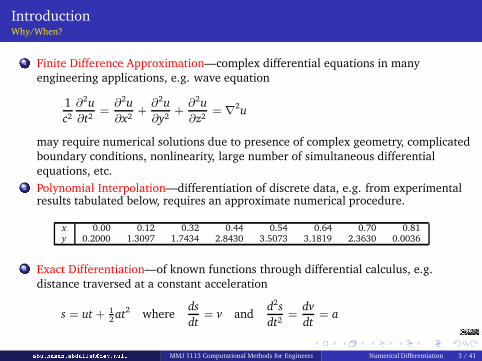
IntroductionWhy/When?
1 Finite Difference Approximation—complex differential equations in many
engineering applications, e.g. wave equation
1
c2
∂2u
∂t2=
∂2u
∂x2+
∂2u
∂y2+
∂2u
∂z2= ∇
2u
may require numerical solutions due to presence of complex geometry, complicated
boundary conditions, nonlinearity, large number of simultaneous differential
equations, etc.
2 Polynomial Interpolation—differentiation of discrete data, e.g. from experimentalresults tabulated below, requires an approximate numerical procedure.
x 0.00 0.12 0.32 0.44 0.54 0.64 0.70 0.81y 0.2000 1.3097 1.7434 2.8430 3.5073 3.1819 2.3630 0.0036
3 Exact Differentiation—of known functions through differential calculus, e.g.
distance traversed at a constant acceleration
s = ut + 12at2 where
ds
dt= v and
d2s
dt2=
dv
dt= aabu.hasan.abdullah�dev.null MMJ 1113 Computational Methods for Engineers Numerical Differentiation 3 / 41
IntroductionFinite Difference Approximation
Differential equations in many engineering applications require numericalsolutions due to
presence of complex geometry and/or complicated boundary conditionsnonlinearity and/or large number of simultaneous differential equations, etc.
Derivatives in these differential equations are replaced by their discrete forms,
known as finite-difference approximations. Use of finite-differences transforms an
ordinary differential equation into an algebraic equation
Taylor series used in computing derivatives using discrete methods is cumbersome
for approximations of increasingly high accuracy or higher-order derivatives
abu.hasan.abdullah�dev.null MMJ 1113 Computational Methods for Engineers Numerical Differentiation 4 / 41

IntroductionPolynomial Interpolation
If a function is very complicated or
known only from values in a table (e.g.
from experiments), it may be necessary
to resort to numerical differentiation.
In cases especially where data are
obtained experimentally it is best to
perform a least squares curve fit to
data and then find the resulting
polynomial.
Formulae for numerical differentiation
may easily be obtained by
differentiating interpolation
polynomials. The essential idea is that
the derivatives f ′, f ′′, . . . of a function
are represented by the derivatives P′
n,
P′′
n , . . . of the interpolating polynomial
Pn—more on this towards the end!Figure 1 : Interpolating polynomial.abu.hasan.abdullah�dev.null MMJ 1113 Computational Methods for Engineers Numerical Differentiation 5 / 41
IntroductionErrors in Numerical Differentiation
Numerical differentiation is avoided wherever it is possible because of several inherent
difficulties:
1 Integration describes an overall property of a function, whereas differentiation
describes the slope of a function at a point. Integration is not sensitive to minor
changes in the shape of a function, whereas differentiation is. Any small changes in
a function can easily create large changes in its slope in the neighborhood of the
change. Compared to integration, numerical differentiation is less reliable.
2 Large errors may also occur in numerical differentiation based on Taylor series,
which is cumbersome for approximations of high accuracy or higher-order
derivatives.
abu.hasan.abdullah�dev.null MMJ 1113 Computational Methods for Engineers Numerical Differentiation 6 / 41
Sample Engineering ProblemsProblem 1
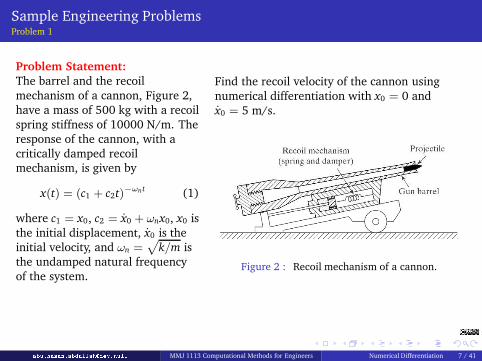
Problem Statement:
The barrel and the recoil
mechanism of a cannon, Figure 2,
have a mass of 500 kg with a recoil
spring stiffness of 10000 N/m. The
response of the cannon, with a
critically damped recoil
mechanism, is given by
x(t) = (c1 + c2t)−ωnt(1)
where c1 = x0, c2 = x0 + ωnx0, x0 is
the initial displacement, x0 is the
initial velocity, and ωn =p
k/m is
the undamped natural frequency
of the system.
Find the recoil velocity of the cannon using
numerical differentiation with x0 = 0 and
x0 = 5 m/s.
Figure 2 : Recoil mechanism of a cannon.
abu.hasan.abdullah�dev.null MMJ 1113 Computational Methods for Engineers Numerical Differentiation 7 / 41
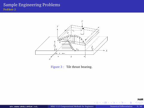
Sample Engineering ProblemsProblem 2
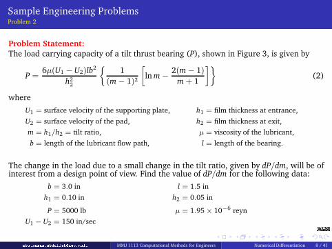
Problem Statement:
The load carrying capacity of a tilt thrust bearing (P), shown in Figure 3, is given by
P =6µ(U1 − U2)lb
2
h22
1
(m − 1)2
»
ln m −2(m − 1)
m + 1
–ff
(2)
where
U1 = surface velocity of the supporting plate, h1 = film thickness at entrance,
U2 = surface velocity of the pad, h2 = film thickness at exit,
m = h1/h2 = tilt ratio, µ = viscosity of the lubricant,
b = length of the lubricant flow path, l = length of the bearing.
The change in the load due to a small change in the tilt ratio, given by dP/dm, will be ofinterest from a design point of view. Find the value of dP/dm for the following data:
b = 3.0 in l = 1.5 in
h1 = 0.10 in h2 = 0.05 in
P = 5000 lb µ = 1.95 × 10⁻⁶ reyn
U1 − U2 = 150 in/secabu.hasan.abdullah�dev.null MMJ 1113 Computational Methods for Engineers Numerical Differentiation 8 / 41
Sample Engineering ProblemsProblem 2
Figure 3 : Tilt thrust bearing.
abu.hasan.abdullah�dev.null MMJ 1113 Computational Methods for Engineers Numerical Differentiation 9 / 41
Sample Engineering ProblemsProblem 3
Problem Statement:
The pressure (p)–specific volume (v) relationship of superheated water vapour at 350◦C
is given by van der Waals equation
p =RT
v − b−
a
v2(3)
where
T = absolute temperature = 623.15 K a = 1.7048
R = specific gas constant = 0.461889 kJ/kg-K b = 0.0016895
Expand the pressure in Taylor’s series and estimate the value of p at
v = 0.051, 0.054, and 0.060 assuming that the value of p and its derivatives are known
at v = 0.05.
abu.hasan.abdullah�dev.null MMJ 1113 Computational Methods for Engineers Numerical Differentiation 10 / 41

Derivative Defined
Derivative of a function f(x) is defined as
df(x)
dx
˛˛˛˛x
= f′(x) = lim
h→0
f(x + h) − f(x)
h
(4)
h does not approach zero but remains a
finite quantity. As h = ∆x, Eq. (4) can
also be written as
f′(x) ≈
f(x + ∆x) − f(x)
∆x(5)
Figure 4 : Derivative defined.
abu.hasan.abdullah�dev.null MMJ 1113 Computational Methods for Engineers Numerical Differentiation 11 / 41
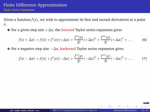
Finite Difference ApproximationTaylor Series Expansions
Given a function f(x), we wish to approximate its first and second derivatives at a point
x.
For a given step size +∆x, the forward Taylor series expansion gives
f(x + ∆x) = f(x) + f′(x)(+∆x) +
f ′′(x)
2!(+∆x)2 +
f ′′′(x)
3!(+∆x)3 + . . . (6)
For a negative step size −∆x, backward Taylor series expansion gives
f(x − ∆x) = f(x) + f′(x)(−∆x) +
f ′′(x)
2!(−∆x)2 +
f ′′′(x)
3!(−∆x)3 + . . . (7)
abu.hasan.abdullah�dev.null MMJ 1113 Computational Methods for Engineers Numerical Differentiation 12 / 41

Finite Difference ApproximationApproximating First Derivative to O(h) Accuracy
Solving Eq. (6) for (df(x)/dx)i,j
df(x)
dx= f
′(x) =f(x + ∆x) − f(x)
∆x| {z }
finite difference
−f ′′
2!(∆x) −
f ′′′
3!(∆x)2
− . . .| {z }
truncation error, O(∆x)
=f(x + ∆x) − f(x)
∆x+ O(∆x)
For ∆x = h and ignoring
O(∆x), we get a forward
difference formula
f′(x) ≈
f(x + h) − f(x)
h(8)
which is first-order accurate.
Figure 5 : Forward difference formulation.abu.hasan.abdullah�dev.null MMJ 1113 Computational Methods for Engineers Numerical Differentiation 13 / 41
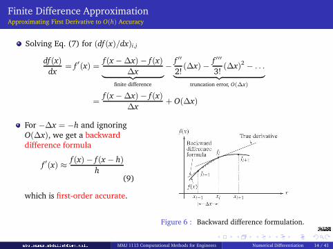
Finite Difference ApproximationApproximating First Derivative to O(h) Accuracy
Solving Eq. (7) for (df(x)/dx)i,j
df(x)
dx= f
′(x) =f(x − ∆x) − f(x)
∆x| {z }
finite difference
−f ′′
2!(∆x) −
f ′′′
3!(∆x)2
− . . .| {z }
truncation error, O(∆x)
=f(x − ∆x) − f(x)
∆x+ O(∆x)
For −∆x = −h and ignoring
O(∆x), we get a backward
difference formula
f′(x) ≈
f(x) − f(x − h)
h(9)
which is first-order accurate.
Figure 6 : Backward difference formulation.abu.hasan.abdullah�dev.null MMJ 1113 Computational Methods for Engineers Numerical Differentiation 14 / 41

Finite Difference ApproximationApproximating First Derivative to O(h2) Accuracy
Substract Eq. (7) from Eq. (6) to
give centred difference formula for
f ′(x)
f′(x) =
f(x + h) − f(x − h)
2h
−f ′′′(x)
3!h
2 + . . .
≈f(x + h) − f(x − h)
2h(10)
which is second-order accurate.
Figure 7 : Central difference formulation.
abu.hasan.abdullah�dev.null MMJ 1113 Computational Methods for Engineers Numerical Differentiation 15 / 41
Finite Difference ApproximationApproximating Second Derivative to O(h2) Accuracy
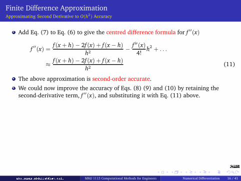
Add Eq. (7) to Eq. (6) to give the centred difference formula for f ′′(x)
f′′(x) =
f(x + h) − 2f(x) + f(x − h)
h2−
f iv(x)
4!h
2 + . . .
≈f(x + h) − 2f(x) + f(x − h)
h2(11)
The above approximation is second-order accurate.
We could now improve the accuracy of Eqs. (8) (9) and (10) by retaining the
second-derivative term, f ′′(x), and substituting it with Eq. (11) above.
abu.hasan.abdullah�dev.null MMJ 1113 Computational Methods for Engineers Numerical Differentiation 16 / 41

Finite Difference ApproximationCentred Difference Formulae of Orders O(h2) and O(h4)
Centred Difference Formulae of Order O(h2)
f′(x) ≈
f(x + h) − f(x − h)
2h(12)
f′′(x) ≈
f(x + h) − 2f(x) + f(x − h)
h2(13)
f′′′
(x) ≈
f(x + 2h) − f(x + h) + 2f(x − h) − f(x − 2h)
2h3(14)
f(4)
(x) ≈
f(x + 2h) − 4f(x + h) + 6f(x) − 4f(x − h) + f(x − 2h)
h4(15)
Centred Difference Formulae of Order O(h4)
f′(x) ≈
−f(x + 2h) + 8f(x + h) − 8f(x − h) + f(x − 2h)
12h(16)
f′′(x) ≈
−f(x + 2h) + 16f(x + h) − 30f(x) + 16f(x − h) − f(x − 2h)
12h2(17)
f′′′
(x) ≈
−f(x + 3h) + 8f(x + 2h) − 13f(x + h) + 13f(x − h) − 8f(x − 2h) + f(x − 3h)
8h3(18)
f(4)
(x) ≈
−f(x + 3h) + 12f(x + 2h) − 39f(x + h) + 56f(x) − 39f(x − h) + 12f(x − 2h) − f(x − 3h)
6h4(19)abu.hasan.abdullah�dev.null MMJ 1113 Computational Methods for Engineers Numerical Differentiation 17 / 41

Finite Difference ApproximationImproving Derivative Estimates–Richardson Extrapolation
Two approaches normally used to improve derivative estimates
decrease step size huse higher-order formula that employs more points
There is also a third approach–Richardson extrapolation–a method often used to
improve the results of a numerical method, from a method of order O(hn) it gives
us a method of order O(hn+1). Richardson extrapolation uses two derivatives to
compute a third, more accurate approximation.
In integration, Richardson extrapolation provides a means to obtain an improved
integral estimate I by formula
I ≈ I(h2) +1
„h1
h2
«2
− 1
[I(h2) − I(h1)] (20)
where I(h1) and I(h2) are integral estimates using two step sizes h1 and h2.
Eq. (20) is usually written for the case where h2 = 12h1 to give
I ≈4
3I(h2) −
1
3I(h1) (21)abu.hasan.abdullah�dev.null MMJ 1113 Computational Methods for Engineers Numerical Differentiation 18 / 41
Finite Difference ApproximationImproving Derivative Estimates–Richardson Extrapolation
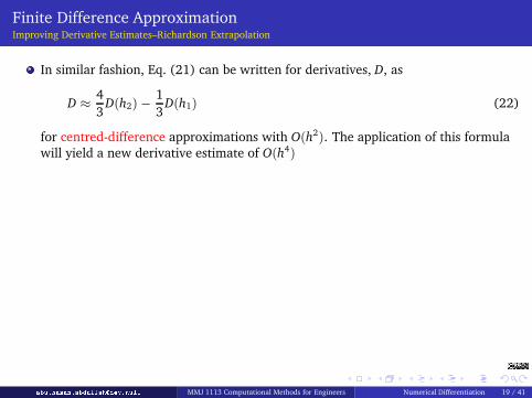
In similar fashion, Eq. (21) can be written for derivatives, D, as
D ≈4
3D(h2) −
1
3D(h1) (22)
for centred-difference approximations with O(h2). The application of this formula
will yield a new derivative estimate of O(h4)
abu.hasan.abdullah�dev.null MMJ 1113 Computational Methods for Engineers Numerical Differentiation 19 / 41

Finite Difference ApproximationCentred Difference Formulae–Example 1
Problem Statement:
Let f(x) = sin(x), where x is measured in radians.
1 Calculate approximations to f ′(0.8) using the centred difference formula of order
O(h2) with ∆x = h = 0.1, ∆x = h = 0.01, ∆x = h = 0.001. Carry eight or nine
decimal places.
2 Compare with the value f ′(0.8) = cos(0.8).
Solution:
Work through the example.
abu.hasan.abdullah�dev.null MMJ 1113 Computational Methods for Engineers Numerical Differentiation 20 / 41
Finite Difference ApproximationCentred Difference Formulae–Example 2
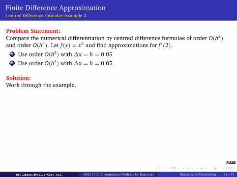
Problem Statement:
Compare the numerical differentiation by centred difference formulae of order O(h2)and order O(h4). Let f(x) = x3 and find approximations for f ′(2).
1 Use order O(h2) with ∆x = h = 0.05
2 Use order O(h4) with ∆x = h = 0.05
Solution:
Work through the example.
abu.hasan.abdullah�dev.null MMJ 1113 Computational Methods for Engineers Numerical Differentiation 21 / 41
Finite Difference ApproximationCentred Difference Formulae–Example 3 (Programming)
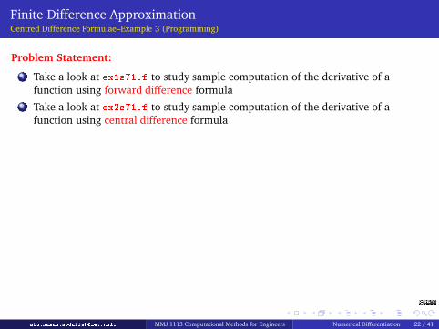
Problem Statement:
1 Take a look at ex1s71.f to study sample computation of the derivative of a
function using forward difference formula
2 Take a look at ex2s71.f to study sample computation of the derivative of a
function using central difference formula
abu.hasan.abdullah�dev.null MMJ 1113 Computational Methods for Engineers Numerical Differentiation 22 / 41

Finite Difference ApproximationCentred Difference Formulae–Example 4 (Richardson extrapolation)
Problem Statement:
Using the function
f(x) = −0.1x4− 0.15x
3− 0.5x
2− 0.25x + 1.2
estimate the first derivative at x = 0.5 employing step sizes h1 = 0.5 and h2 = 0.25.
Compute an improved estimate with Richardson extrapolation. As a comparison, the
true value is −0.9125.
Solution:
Work through the example.
abu.hasan.abdullah�dev.null MMJ 1113 Computational Methods for Engineers Numerical Differentiation 23 / 41
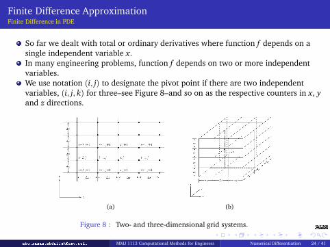
Finite Difference ApproximationFinite Difference in PDE
So far we dealt with total or ordinary derivatives where function f depends on a
single independent variable x.
In many engineering problems, function f depends on two or more independent
variables.
We use notation (i, j) to designate the pivot point if there are two independent
variables, (i, j, k) for three–see Figure 8–and so on as the respective counters in x, y
and z directions.
(a) (b)
Figure 8 : Two- and three-dimensional grid systems.abu.hasan.abdullah�dev.null MMJ 1113 Computational Methods for Engineers Numerical Differentiation 24 / 41

Finite Difference ApproximationFinite Difference in PDE
Consider f(x, y). Finite-difference approximation for the partial derivative
∂f(x, y)
∂xat (x = xi, y = yj)
can be found by fixing value of y at yj and treat f(x, yj) as a one-variable function.
Forward-difference approximation of ∂f/∂x is
∂f
∂x
˛˛˛˛i,j
≈f(xi + ∆x, yj) − f(xi, yj)
∆x(23)
Backward-difference approximation of ∂f/∂x is
∂f
∂y
˛˛˛˛i,j
≈f(xi, yj) − f(xi − ∆x, yj)
∆x(24)
Central-difference approximation of ∂f/∂x is
∂f
∂y
˛˛˛˛i,j
≈f(xi + ∆x, yj) − f(xi − ∆x, yj)
2∆x(25)abu.hasan.abdullah�dev.null MMJ 1113 Computational Methods for Engineers Numerical Differentiation 25 / 41
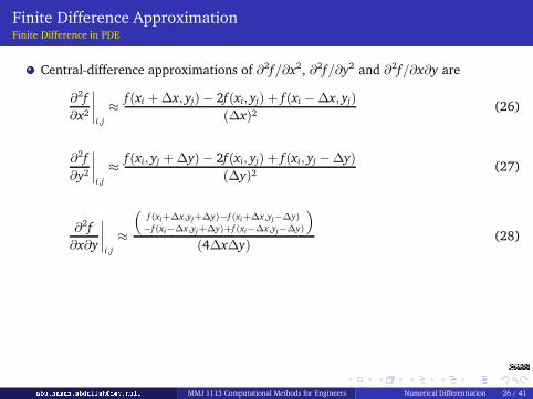
Finite Difference ApproximationFinite Difference in PDE
Central-difference approximations of ∂2f/∂x2, ∂2f/∂y2 and ∂2f/∂x∂y are
∂2f
∂x2
˛˛˛˛i,j
≈f(xi + ∆x, yj) − 2f(xi, yj) + f(xi − ∆x, yj)
(∆x)2(26)
∂2f
∂y2
˛˛˛˛i,j
≈f(xi, yj + ∆y) − 2f(xi, yj) + f(xi, yj − ∆y)
(∆y)2(27)
∂2f
∂x∂y
˛˛˛˛i,j
≈
“f(xi+∆x,yj+∆y)−f(xi+∆x,yj−∆y)
−f(xi−∆x,yj+∆y)+f(xi−∆x,yj−∆y)
”
(4∆x∆y)(28)
abu.hasan.abdullah�dev.null MMJ 1113 Computational Methods for Engineers Numerical Differentiation 26 / 41

Polynomial Interpolation
The function f(x), which is to be differentiated, may be
a known function, ora set of discrete data.
In general, known functions can be differentiated exactly.
Differentiation of discrete data, however, requires an approximate numerical
procedure. To perform numerical differentiation, an approximating polynomial is
fit to the discrete data, or a subset of the discrete data, and the approximating
polynomial is differentiated.
We’ll look at differentiation of1 direct fit polynomials,2 Lagrange polynomials, and3 divided difference polynomials
which can be applied to both unequally spaced data and equally spaced data.
abu.hasan.abdullah�dev.null MMJ 1113 Computational Methods for Engineers Numerical Differentiation 27 / 41
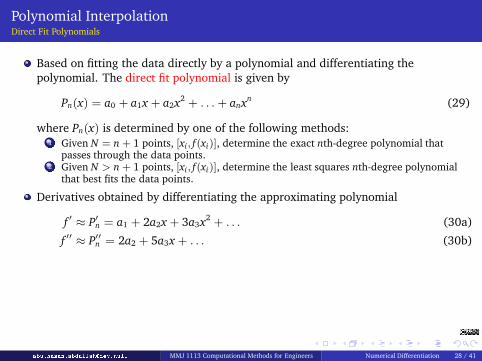
Polynomial InterpolationDirect Fit Polynomials
Based on fitting the data directly by a polynomial and differentiating the
polynomial. The direct fit polynomial is given by
Pn(x) = a0 + a1x + a2x2 + . . . + anx
n(29)
where Pn(x) is determined by one of the following methods:1 Given N = n + 1 points, [xi, f(xi)], determine the exact nth-degree polynomial that
passes through the data points.2 Given N > n + 1 points, [xi, f(xi)], determine the least squares nth-degree polynomial
that best fits the data points.
Derivatives obtained by differentiating the approximating polynomial
f′
≈ P′
n = a1 + 2a2x + 3a3x2 + . . . (30a)
f′′
≈ P′′
n = 2a2 + 5a3x + . . . (30b)
abu.hasan.abdullah�dev.null MMJ 1113 Computational Methods for Engineers Numerical Differentiation 28 / 41
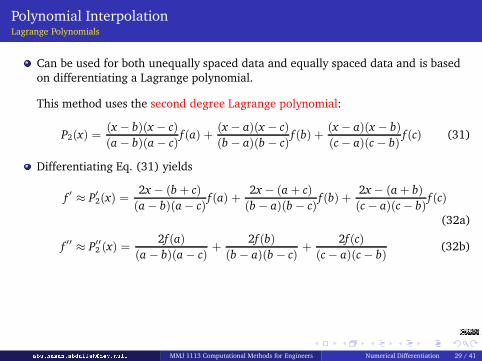
Polynomial InterpolationLagrange Polynomials
Can be used for both unequally spaced data and equally spaced data and is based
on differentiating a Lagrange polynomial.
This method uses the second degree Lagrange polynomial:
P2(x) =(x − b)(x − c)
(a − b)(a − c)f(a) +
(x − a)(x − c)
(b − a)(b − c)f(b) +
(x − a)(x − b)
(c − a)(c − b)f(c) (31)
Differentiating Eq. (31) yields
f′
≈ P′
2(x) =2x − (b + c)
(a − b)(a − c)f(a) +
2x − (a + c)
(b − a)(b − c)f(b) +
2x − (a + b)
(c − a)(c − b)f(c)
(32a)
f′′
≈ P′′
2 (x) =2f(a)
(a − b)(a − c)+
2f(b)
(b − a)(b − c)+
2f(c)
(c − a)(c − b)(32b)
abu.hasan.abdullah�dev.null MMJ 1113 Computational Methods for Engineers Numerical Differentiation 29 / 41
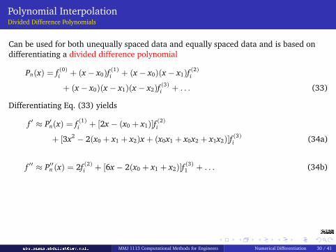
Polynomial InterpolationDivided Difference Polynomials
Can be used for both unequally spaced data and equally spaced data and is based on
differentiating a divided difference polynomial
Pn(x) = f(0)i + (x − x0)f
(1)i + (x − x0)(x − x1)f
(2)i
+ (x − x0)(x − x1)(x − x2)f(3)i + . . . (33)
Differentiating Eq. (33) yields
f′
≈ P′
n(x) = f(1)i + [2x − (x0 + x1)]f
(2)i
+ [3x2− 2(x0 + x1 + x2)x + (x0x1 + x0x2 + x1x2)]f
(3)i (34a)
f′′
≈ P′′
n (x) = 2f(2)i + [6x − 2(x0 + x1 + x2)]f
(3)1 + . . . (34b)
abu.hasan.abdullah�dev.null MMJ 1113 Computational Methods for Engineers Numerical Differentiation 30 / 41
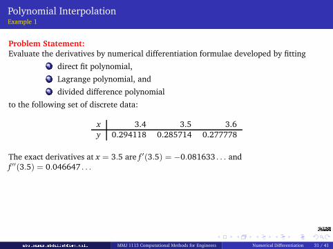
Polynomial InterpolationExample 1
Problem Statement:
Evaluate the derivatives by numerical differentiation formulae developed by fitting
1 direct fit polynomial,
2 Lagrange polynomial, and
3 divided difference polynomial
to the following set of discrete data:
x 3.4 3.5 3.6
y 0.294118 0.285714 0.277778
The exact derivatives at x = 3.5 are f ′(3.5) = −0.081633 . . . and
f ′′(3.5) = 0.046647 . . .
abu.hasan.abdullah�dev.null MMJ 1113 Computational Methods for Engineers Numerical Differentiation 31 / 41
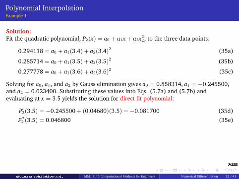
Polynomial InterpolationExample 1
Solution:
Fit the quadratic polynomial, P2(x) = a0 + a1x + a2x22, to the three data points:
0.294118 = a0 + a1(3.4) + a2(3.4)2(35a)
0.285714 = a0 + a1(3.5) + a2(3.5)2(35b)
0.277778 = a0 + a1(3.6) + a2(3.6)2(35c)
Solving for a0, a1, and a2 by Gauss elimination gives a0 = 0.858314, a1 = −0.245500,
and a2 = 0.023400. Substituting these values into Eqs. (5.7a) and (5.7b) and
evaluating at x = 3.5 yields the solution for direct fit polynomial:
P′
2(3.5) = −0.245500 + (0.04680)(3.5) = −0.081700 (35d)
P′′
2 (3.5) = 0.046800 (35e)
abu.hasan.abdullah�dev.null MMJ 1113 Computational Methods for Engineers Numerical Differentiation 32 / 41
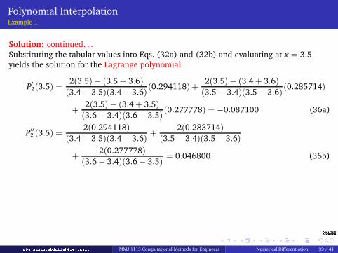
Polynomial InterpolationExample 1
Solution: continued. . .
Substituting the tabular values into Eqs. (32a) and (32b) and evaluating at x = 3.5yields the solution for the Lagrange polynomial
P′
2(3.5) =2(3.5) − (3.5 + 3.6)
(3.4 − 3.5)(3.4 − 3.6)(0.294118) +
2(3.5) − (3.4 + 3.6)
(3.5 − 3.4)(3.5 − 3.6)(0.285714)
+2(3.5) − (3.4 + 3.5)
(3.6 − 3.4)(3.6 − 3.5)(0.277778) = −0.087100 (36a)
P′′
2 (3.5) =2(0.294118)
(3.4 − 3.5)(3.4 − 3.6)+
2(0.283714)
(3.5 − 3.4)(3.5 − 3.6)
+2(0.277778)
(3.6 − 3.4)(3.6 − 3.5)= 0.046800 (36b)
abu.hasan.abdullah�dev.null MMJ 1113 Computational Methods for Engineers Numerical Differentiation 33 / 41
Polynomial InterpolationExample 1
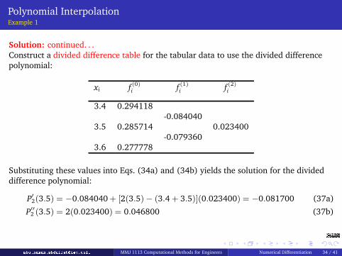
Solution: continued. . .
Construct a divided difference table for the tabular data to use the divided difference
polynomial:
xi f(0)i f
(1)i f
(2)i
3.4 0.294118
-0.084040
3.5 0.285714 0.023400
-0.079360
3.6 0.277778
Substituting these values into Eqs. (34a) and (34b) yields the solution for the divided
difference polynomial:
P′
2(3.5) = −0.084040 + [2(3.5) − (3.4 + 3.5)](0.023400) = −0.081700 (37a)
P′′
2 (3.5) = 2(0.023400) = 0.046800 (37b)abu.hasan.abdullah�dev.null MMJ 1113 Computational Methods for Engineers Numerical Differentiation 34 / 41

Polynomial InterpolationExample 1
Solution: continued. . .
The results obtained by the three procedures are identical since the same three points
are used in all three procedures.
The error in f ′(3.5) is
Error = f′(3.5) − P
′
2(3.5)
= −0.081700− (−0.081633)
= −0.000067
The error in f ′′(3.5) is
Error = f′′(3.5) − P
′′
2 (3.5)
= 0.046800− 0.046647
= 0.000153
abu.hasan.abdullah�dev.null MMJ 1113 Computational Methods for Engineers Numerical Differentiation 35 / 41
Polynomial InterpolationExample 2: Using Matlab
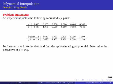
Problem Statement:
An experiment yields the following tabulated x-y pairs:
x 0.000 0.100 0.200 0.300 0.400 0.500
y -0.447 1.978 3.280 6.160 7.080 7.340
x (cont. . . ) 0.600 0.700 0.800 0.900 1.000
y (cont. . . ) 7.660 9.560 9.480 9.300 11.20
Perform a curve fit to the data and find the approximating polynomial. Determine the
derivative at x = 0.5.
abu.hasan.abdullah�dev.null MMJ 1113 Computational Methods for Engineers Numerical Differentiation 36 / 41
Polynomial InterpolationExample 2: Using Matlab
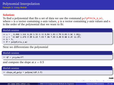
Solution:
To find a polynomial that fits a set of data we use the command polyfit(x,y,n),where x is a vector containing x-axis values, y is a vector containing y-axis values and nis the order of the polynomial that we want to fit:
Matlab session>> x = [ 0.000 0.100 0.20 0.30 0.40 0.50 0.60 0.70 0.80 0.90 1.00℄;>> y = [-0.447 1.978 3.28 6.16 7.08 7.34 7.66 9.56 9.48 9.30 11.2℄;>> n = 2;>> P = polyfit(x,y,n)Next we differentiate the polynomial
Matlab session>> dP = polyder(P)and compute the slope at x = 0.5
Matlab session>> slope_of_poly = polyval(dP,0.5)abu.hasan.abdullah�dev.null MMJ 1113 Computational Methods for Engineers Numerical Differentiation 37 / 41
Polynomial InterpolationExample 2: Using Matlab
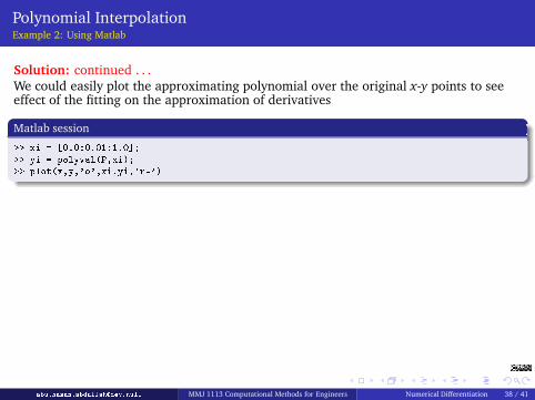
Solution: continued . . .
We could easily plot the approximating polynomial over the original x-y points to seeeffect of the fitting on the approximation of derivatives
Matlab session>> xi = [0.0:0.01:1.0℄;>> yi = polyval(P,xi);>> plot(x,y,'o',xi,yi,'r-')
abu.hasan.abdullah�dev.null MMJ 1113 Computational Methods for Engineers Numerical Differentiation 38 / 41

Polynomial InterpolationExample 3: Using Matlab
Problem Statement:
An experiment yields unequally spaced data in x and y
x y x y x y
0.00 0.2000 0.36 2.0749 0.64 3.18190.12 1.3097 0.40 2.4560 0.70 2.36300.22 1.3052 0.44 2.8430 0.80 0.23200.32 1.7434 0.54 3.5073 0.81 0.0036
Determine the differences between adjacent elements of both x and y vectors and
compute divided-difference approximations of the derivative.
abu.hasan.abdullah�dev.null MMJ 1113 Computational Methods for Engineers Numerical Differentiation 39 / 41

Polynomial InterpolationExample 3: Using Matlab
Solution:
To differentiate unequally spaced data in x and y we use the command diff(x) anddiff(y), where x is a vector containing x values, y is a vector containing y values
Matlab session>> diff(x);>> diff(y);To compute divided-difference approximations of the derivative we perform vectordivision of y differences by x differences
Matlab session>> dydx = diff(y)./diff(x)abu.hasan.abdullah�dev.null MMJ 1113 Computational Methods for Engineers Numerical Differentiation 40 / 41
Bibliography
1 SINGIRESU S. RAO (2002): Applied Numerical Methods for Engineers and Scientists, ISBN0-13-089480-X, Prentice Hall
2 STEVEN C. CHAPRA, RAYMOND P. CANALE (2006): Numerical Methods for Engineers, 5ed,ISBN 007-124429-8, McGraw-Hill
3 DAVID KINCAID AND WARD CHENEY (1991): Numerical Analysis: Mathematics of ScientificComputing, ISBN 0-534-13014-3, Brooks/Cole Publishing Co.
4 STEVEN C. CHAPRA (2005): Applied Numerical Methods with MATLAB for Engineers andScientists, ISBN 007-124484-0, McGraw-Hill
5 WILLIAM J. PALM III (2005): Introduction to Matlab 7 for Engineers, ISBN 007-123262-1,McGraw-Hill
6 JOHN D. ANDERSON, JR. (1995): Computational Fluid Dynamics–The Basics withApplications, ISBN 007-113210-4, McGraw-Hill
abu.hasan.abdullah�dev.null MMJ 1113 Computational Methods for Engineers Numerical Differentiation 41 / 41