€¦ · 2 Gravity ﬁeld of the earth 2.1 Gravity Thetotal force acting on a bodyat rest on the...

2 Gravity field of the earth

2.1 Gravity

The total force acting on a body at rest on the earth’s surface is the resultantof gravitational force and the centrifugal force of the earth’s rotation and iscalled gravity.

Take a rectangular coordinate system whose origin is at the earth’s centerof gravity and whose z-axis coincides with the earth’s mean axis of rotation(Fig. 2.1). The x- and y-axes are so chosen as to obtain a right-handedcoordinate system; otherwise they are arbitrary. For convenience, we mayassume an x-axis which is associated with the mean Greenwich meridian (it“points” towards the mean Greenwich meridian). Note that we are assumingin this book that the earth is a solid body rotating with constant speedaround a fixed axis. This is a rather simplified assumption, see Moritz andMueller (1987). The centrifugal force f on a unit mass is given by

f = ω2p , (2–1)

where ω is the angular velocity of the earth’s rotation and

p =√

x2 + y2 (2–2)

is the distance from the axis of rotation. The vector f of this force has the

Pp

x

y p

x

y

z

f

!

Fig. 2.1. The centrifugal force

44 2 Gravity field of the earth

direction of the vectorp = [x, y, 0] (2–3)

and is, therefore, given by

f = ω2p = [ω2x, ω2y, 0] . (2–4)

The centrifugal force can also be derived from a potential

Φ =12

ω2(x2 + y2) , (2–5)

so that

f = grad Φ ≡[∂Φ∂x

,∂Φ∂y

,∂Φ∂z

]. (2–6)

Substituting (2–5) into (2–6) yields (2–4).In the introductory remark above, we mentioned that gravity is the resul-

tant of gravitational force and centrifugal force. Accordingly, the potential ofgravity, W , is the sum of the potentials of gravitational force, V , cf. (1–12),and centrifugal force, Φ:

W = W (x, y, z) = V + Φ = G

∫∫v

∫�

ldv +

12

ω2(x2 + y2) , (2–7)

where the integration is extended over the earth.Differentiating (2–5), we find

∆Φ ≡ ∂2Φ∂x2

+∂2Φ∂y2

+∂2Φ∂z2

= 2ω2 . (2–8)

If we combine this with Poisson’s equation (1–17) for V , we get the general-ized Poisson equation for the gravity potential W :

∆W = −4π G� + 2ω2 . (2–9)

Since Φ is an analytic function, the discontinuities of W are those of V : somesecond derivatives have jumps at discontinuities of density.

The gradient vector of W ,

g = grad W ≡[∂W

∂x,

∂W

∂y,

∂W

∂z

](2–10)

2.1 Gravity 45

with components

gx =∂W

∂x= −G

∫∫v

∫x − ξ

l3� dv + ω2x ,

gy =∂W

∂y= −G

∫∫v

∫y − η

l3� dv + ω2y ,

gz =∂W

∂z= −G

∫∫v

∫z − ζ

l3� dv ,

(2–11)

is called the gravity vector ; it is the total force (gravitational force pluscentrifugal force) acting on a unit mass. As a vector, it has magnitude anddirection.

The magnitude g is called gravity in the narrower sense. It has the phys-ical dimension of an acceleration and is measured in gal (1 gal = 1 cm s−2),the unit being named in honor of Galileo Galilei. The numerical value of gis about 978 gal at the equator, and 983 gal at the poles. In geodesy, anotherunit is often convenient – the milligal, abbreviated mgal (1 mgal = 10−3 gal).

In SI units, we have

1 gal = 0.01 m s−2 ,

1 mgal = 10µm s−2 .(2–12)

The direction of the gravity vector is the direction of the plumb line, or thevertical; its basic significance for geodetic and astronomical measurementsis well known.

In addition to the centrifugal force, another force called the Coriolis forceacts on a moving body. It is proportional to the velocity with respect to theearth, so that it is zero for bodies resting on the earth. Since in classicalgeodesy (i.e., not considering navigation) we usually deal with instrumentsat rest relative to the earth, the Coriolis force plays no role here and neednot be considered.

Gravitational and inertial massThe reader may have noticed that the mass m has been used in two con-ceptually completely different senses: as inertial mass in Newton’s law ofinertia, force=mass×acceleration and as gravitational mass in Newton’slaw of gravitation (1–1). Thus, m in gravitation, which is a “true” force, isthe gravitational mass, but m in the centrifugal “force”, which is an accel-eration, is the inertial mass. The Hungarian physicist Roland Eotvos hadshown experimentally already around 1890 that both kinds of masses are


equal within 10−11, which is a formidable accuracy. He used the same typeof instrument by which experimental physicists have been able to determinethe numerical value of the gravitational constant G only to a poor accuracyof about 10−4, as we have seen at the beginning of this book. The coinci-dence between the inertial and the gravitational mass was far too good to bea physical accident, but, within classical mechanics, it was an inexplicablemiracle. It was not before 1915 that Einstein made it one of the pillars ofthe general theory of relativity!

2.2 Level surfaces and plumb lines

The surfacesW (x, y, z) = constant , (2–13)

on which the potential W is constant, are called equipotential surfaces orlevel surfaces.

Differentiating the gravity potential W = W (x, y, z), we find

dW =∂W

∂xdx +

∂W

∂ydy +

∂W

∂zdz . (2–14)

In vector notation, using the scalar product, this reads

dW = grad W · dx = g · dx , (2–15)

wheredx = [dx, dy, dz] . (2–16)

If the vector dx is taken along the equipotential surface W = constant, thenthe potential remains constant and dW = 0, so that (2–15) becomes

g · dx = 0 . (2–17)

If the scalar product of two vectors is zero, then these vectors are orthogonalto each other. This equation therefore expresses the well-known fact that thegravity vector is orthogonal to the equipotential surface passing through thesame point.

The surface of the oceans, after some slight idealization, is part of acertain level surface. This particular equipotential surface was proposed asthe “mathematical figure of the earth” by C.F. Gauss, the “Prince of Mathe-maticians”, and was later termed the geoid. This definition has proved highlysuitable, and the geoid is still frequently considered by many to be the fun-damental surface of physical geodesy. The geoid is thus defined by

W = W0 = constant . (2–18)

2.2 Level surfaces and plumb lines 47

geoid

W W= 0

PH

g

level surfaceW = constant

Fig. 2.2. Level surfaces and plumb lines

If we look at equation (2–7) for the gravity potential W , we can see thatthe equipotential surfaces, expressed by W (x, y, z) = constant, are rathercomplicated mathematically. The level surfaces that lie completely outsidethe earth are at least analytical surfaces, although they have no simple ana-lytical expression, because the gravity potential W is analytical outside theearth. This is not true of level surfaces that are partly or wholly inside theearth, such as the geoid. They are continuous and “smooth” (i.e., withoutedges), but they are no longer analytical surfaces; we will see in the next sec-tion that the curvature of the interior level surfaces changes discontinuouslywith the density.

The lines that intersect all equipotential surfaces orthogonally are notexactly straight but slightly curved (Fig. 2.2). They are called lines of force,or plumb lines. The gravity vector at any point is tangent to the plumb line atthat point, hence “direction of the gravity vector”, “vertical”, and “directionof the plumb line” are synonymous. Sometimes this direction itself is brieflydenoted as “plumb line”.

As the level surfaces are, so to speak, horizontal everywhere, they sharethe strong intuitive and physical significance of the horizontal; and they sharethe geodetic importance of the plumb line because they are orthogonal toit. Thus, we understand why so much attention is paid to the equipotentialsurfaces.

The height H of a point above sea level (also called the orthometricheight) is measured along the curved plumb line, starting from the geoid


(Fig. 2.2). If we take the vector dx along the plumb line, in the direction ofincreasing height H, then its length will be

‖dx‖ = dH (2–19)

and its direction is opposite to the gravity vector g, which points downward,so that the angle between dx and g is 180◦. Using the definition of the scalarproduct (i.e., for two vectors a and b it is defined as a · b = ‖a‖‖b‖ cos ω,where ω is the angle between the two vectors), we get

g · dx = g dH cos 180◦ = −g dH (2–20)

accordingly, so that Eq. (2–15) becomes

dW = −g dH . (2–21)

This equation relates the height H to the potential W and will be basic forthe theory of height determination (Chap. 4). It shows clearly the insepara-ble interrelation that characterizes geodesy – the interrelation between thegeometrical concepts (H) and the dynamic concepts (W ).

Another form of Eq. (2–21) is

g = −∂W

∂H. (2–22)

It shows that gravity is the negative vertical gradient of the potential W , orthe negative vertical component of the gradient vector grad W .

Since geodetic measurements (theodolite measurements, leveling, butalso satellite techniques etc.) are almost exclusively referred to the systemof level surfaces and plumb lines, the geoid plays an essential part. Thus,we see why the aim of physical geodesy has been formulated as the de-termination of the level surfaces of the earth’s gravity field. In a still moreabstract but equivalent formulation, we may also say that physical geodesyaims at the determination of the potential function W (x, y, z). At a firstglance, the reader is probably perplexed about this definition, which is dueto Bruns (1878), but its meaning is easily understood: If the potential W isgiven as a function of the coordinates x, y, z, then we know all level surfacesincluding the geoid; they are given by the equation

W (x, y, z) = constant. (2–23)

2.3 Curvature of level surfaces and plumb lines

The formula for the curvature of a curve y = f(x) is

κ =1�

=y′′

(1 + y′2)3/2, (2–24)

2.3 Curvature of level surfaces and plumb lines 49

y f x= ( )

P

x

||x

y

Fig. 2.3. The curvature of a curve

where κ is the curvature, � is the radius of curvature, and

y′ =dy

dx, y′′ =

d2y

dx2. (2–25)

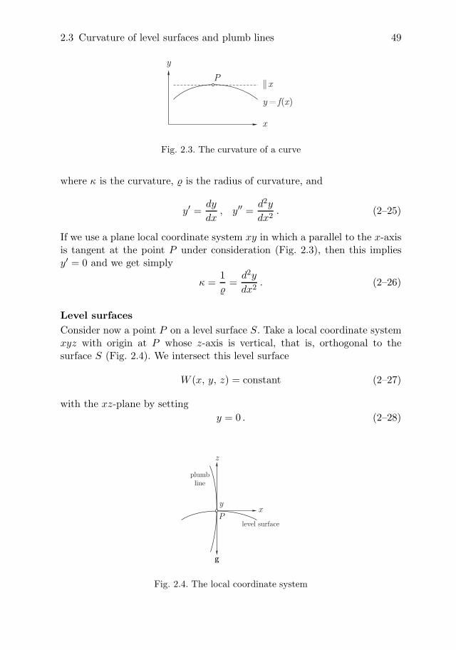
If we use a plane local coordinate system xy in which a parallel to the x-axisis tangent at the point P under consideration (Fig. 2.3), then this impliesy′ = 0 and we get simply

κ =1�

=d2y

dx2. (2–26)

Level surfacesConsider now a point P on a level surface S. Take a local coordinate systemxyz with origin at P whose z-axis is vertical, that is, orthogonal to thesurface S (Fig. 2.4). We intersect this level surface

W (x, y, z) = constant (2–27)

with the xz-plane by settingy = 0 . (2–28)

Px

y

g

z

plumbline

level surface

Fig. 2.4. The local coordinate system


Comparing Fig. 2.4 with Fig. 2.3, we see that z now takes the place ofy. Therefore, instead of (2–26) we have for the curvature of the intersectionof the level surface with the xz-plane:

K1 =d2z

dx2. (2–29)

If we differentiate W (x, y, z) = W0 with respect to x, considering that yis zero and z is a function of x, we get

Wx + Wzdz

dx= 0 ,

Wxx + 2Wxzdz

dx+ Wzz

(dz

dx

)2

+ Wzd2z

dx2= 0 ,

(2–30)

where the subscripts denote partial differentiation:

Wx =∂W

∂x, Wxz =

∂2W

∂x∂z, . . . . (2–31)

Since the x-axis is tangent at P , we get dz/dx = 0 at P , so that

d2z

dx2= −Wxx

Wz. (2–32)

Since the z-axis is vertical, we have, using (2–22),

Wz =∂W

∂z=

∂W

∂H= −g . (2–33)

Therefore, Eq. (2–29) becomes

K1 =Wxx

g. (2–34)

The curvature of the intersection of the level surface with the yz-plane isfound by replacing x with y:

K2 =Wyy

g. (2–35)

The mean curvature J of a surface at a point P is defined as the arith-metic mean of the curvatures of the curves in which two mutually perpen-dicular planes through the surface normal intersect the surface (Fig. 2.5).Hence, we find

J = −12(K1 + K2) = −Wxx + Wyy

2g. (2–36)


P

surface normal

Fig. 2.5. Definition of mean curvature

Here the minus sign is only a convention. This is an expression for the meancurvature of the level surface.

From the generalized Poisson equation

∆W ≡ Wxx + Wyy + Wzz = −4π G� + 2ω2 , (2–37)

we find−2g J + Wzz = −4π G� + 2ω2 . (2–38)

Considering

Wz = −g , Wzz = −∂g

∂z= − ∂g

∂H, (2–39)

we finally obtain∂g

∂H= −2g J + 4π G� − 2ω2 . (2–40)

This important equation, relating the vertical gradient of gravity ∂g/∂H tothe mean curvature of the level surface, is also due to Bruns (1878). It isanother beautiful example of the interrelation between the geometric anddynamic concepts in geodesy.

Plumb linesThe curvature of the plumb line is needed for the reduction of astronomicalobservations to the geoid. A plumb line may be defined as a curve whoseline element vector

dx = [dx, dy, dz] (2–41)

has the direction of the gravity vector

g = [Wx, Wy, Wz] ; (2–42)


that is, dx and g differ only by a proportionality factor. This is best expressedin the form

dx

Wx=

dy

Wy=

dz

Wz. (2–43)

In the coordinate system of Fig. 2.4, the curvature of the projection ofthe plumb line onto the xz-plane is given by

κ1 =d2x

dz2; (2–44)

this is equation (2–26) applied to the present case. Using (2–43), we have

dx

dz=

Wx

Wz. (2–45)

We differentiate with respect to z, considering that y = 0:

d2x

dz2=

1W 2

z

[Wz

(Wxz + Wxx

dx

dz

)− Wx

(Wzz + Wzx

dx

dz

)]. (2–46)

In our particular coordinate system, the gravity vector coincides with thez-axis, so that its x- and y-components are zero:

Wx = Wy = 0 . (2–47)

Figure 2.4 shows that we also have

dx

dz= 0 . (2–48)

Therefore,d2x

dz2=

Wz Wxz

W 2z

=Wxz

Wz=

Wzx

Wz. (2–49)

Considering Wz = −g, we finally obtain

κ1 =1g

∂g

∂x(2–50)

and, similarly,

κ2 =1g

∂g

∂y. (2–51)

These are the curvatures of the projections of the plumb line onto the xz- andyz-plane, the z-axis being vertical, that is, coinciding with the gravity vector.The total curvature κ of the plumb line is given, according to differentialgeometry (essentially Pythagoras’ theorem), by

κ =√

κ21 + κ2

2 =1g

√g2x + g2

y . (2–52)


For reducing astronomical observations (Sect. 5.12), we need only theprojection curvatures (2–50) and (2–51).

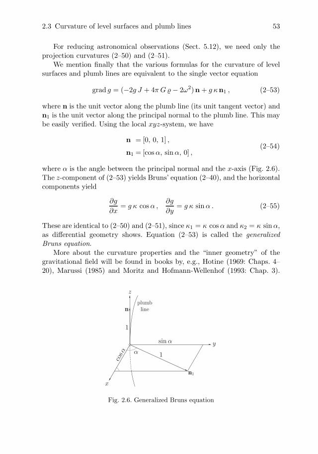
We mention finally that the various formulas for the curvature of levelsurfaces and plumb lines are equivalent to the single vector equation

grad g = (−2g J + 4π G� − 2ω2)n + g κn1 , (2–53)

where n is the unit vector along the plumb line (its unit tangent vector) andn1 is the unit vector along the principal normal to the plumb line. This maybe easily verified. Using the local xyz-system, we have

n = [0, 0, 1] ,

n1 = [cos α, sin α, 0] ,(2–54)

where α is the angle between the principal normal and the x-axis (Fig. 2.6).The z-component of (2–53) yields Bruns’ equation (2–40), and the horizontalcomponents yield

∂g

∂x= g κ cos α ,

∂g

∂y= g κ sin α . (2–55)

These are identical to (2–50) and (2–51), since κ1 = κ cos α and κ2 = κ sin α,as differential geometry shows. Equation (2–53) is called the generalizedBruns equation.

More about the curvature properties and the “inner geometry” of thegravitational field will be found in books by, e.g., Hotine (1969: Chaps. 4–20), Marussi (1985) and Moritz and Hofmann-Wellenhof (1993: Chap. 3).

x

y

z

®

cos®

sin ®

1

plumbline

1

n

n1

Fig. 2.6. Generalized Bruns equation


2.4 Natural coordinates

The system of level surfaces and plumb lines may be used as a three-dimensional curvilinear coordinate system that is well suited to certain pur-poses; these coordinates can be measured directly, as opposed to local rectan-gular coordinates x, y, z. Note, however, that global rectangular coordinatesmay be measured directly using satellites, see Sect. 5.3.

The direction of the earth’s axis of rotation and the position of the equa-torial plane (normal to the axis) are well defined astronomically. The astro-nomical latitude Φ of a point P is the angle between the vertical (directionof the plumb line) at P and the equatorial plane, see Fig. 2.7. From thisfigure, we also see that line PN is parallel to the rotation axis, plane GPFnormal to it, that is, parallel to the equatorial plane; n is the unit vectoralong the plumb line; plane NPF is the meridian plane of P , and planeNPG is parallel to the meridian plane of Greenwich.

Consider now a straight line through P parallel to the earth’s axis ofrotation. This parallel and the vertical at P together define the meridianplane of P . The angle between this meridian plane and the meridian planeof Greenwich (or some other fixed plane) is the astronomical longitude Λ ofP . (Exercise: define Φ and Λ without using the unit sphere. The solutionmay be found in Sect. 5.9).

equator

Gre

enw

ich

mer

idia

n

��

PG

F

vertical

unit sphereN

earth

n

Fig. 2.7. Definition of the astronomical coordinates Φ and Λ of P bymeans of a unit sphere with center at P

2.4 Natural coordinates 55

The astronomical coordinates, latitude Φ and longitude Λ, form two ofthe three spatial coordinates of P . As third coordinate we may take theorthometric height H of P or its potential W . Equivalent to W is the geopo-tential number C = W0 − W , where W0 is the potential of the geoid. Theorthometric height H was defined in Sect. 2.2; see also Fig. 2.2. The relationsbetween W , C, and H are given by the equations

W = W0 −∫ H

0g dH = W0 − C ,

C = W0 − W =∫ H

0g dH ,

H = −∫ W

W0

dW

g=∫ C

0

dC

g,

(2–56)

which follow from integrating (2–21). The integral is taken along the plumbline of point P , starting from the geoid, where H = 0 and W = W0 (see alsoFig. 2.8).

The quantitiesΦ, Λ, W or Φ, Λ, H (2–57)

are called natural coordinates. They are the real-earth counterparts of theellipsoidal coordinates. They are related in the following way to the geocen-tric rectangular coordinates x, y, z of Sect. 2.1. The x-axis is associated withthe mean Greenwich meridian; from Fig. 2.7 we read that the unit vector ofthe vertical n has the xyz-components

n = [cos Φ cos Λ, cos Φ sinΛ, sin Φ] ; (2–58)

the gravity vector g is known to be

g = [Wx, Wy, Wz] . (2–59)

earth's surface

level surfaceP

H

sea level

0geoid

W W= 0

W = constant

Fig. 2.8. The orthometric height H


On the other hand, since n is the unit vector corresponding to g but ofopposite direction, it is given by

n = − g‖g‖ = −g

g, (2–60)

so thatg = −g n . (2–61)

This equation, together with (2–58) and (2–59), gives

−Wx = g cos Φ cos Λ ,

−Wy = g cos Φ sin Λ ,

−Wz = g sin Φ .

(2–62)

Solving for Φ and Λ, we finally obtain

Φ = tan−1 −Wz√W 2

x + W 2y

,

Λ = tan−1 Wy

Wx,

W = W (x, y, z) .

(2–63)

These three equations relate the natural coordinates Φ, Λ, W to the rectan-gular coordinates x, y, z, provided the function W = W (x, y, z) is known.

We see that Φ, Λ, H are related to x, y, z in a considerably more com-plicated way than the spherical coordinates r, ϑ, λ of Sect. 1.4. Note alsothe conceptual difference between the astronomical longitude Λ and the geo-centric longitude λ.

2.5 The potential of the earth in terms of sphericalharmonics

Looking at the expression (2–7) for the gravity potential W , we see that thepart most difficult to handle is the gravitational potential V , the centrifugalpotential being a simple analytic function.

The gravitational potential V can be made more manageable for manypurposes if we keep in mind the fact that outside the attracting masses it isa harmonic function and can therefore be expanded into a series of sphericalharmonics.

2.5 The potential of the earth in terms of spherical harmonics 57

l

P

dM

r

ÃO

r'

Fig. 2.9. Expansion into spherical harmonics

We now evaluate the coefficients of this series. The gravitational potentialV is given by the basic equation (1–12):

V = G

∫∫∫earth

dM

l, (2–64)

where we now denote the mass element by dM ; the integral is extended overthe entire earth. Into this integral we substitute the expression (1–104):

1l

=∞∑

n=0

r′n

rn+1Pn(cos ψ) , (2–65)

where the Pn are the conventional Legendre polynomials, r is the radiusvector of the fixed point P at which V is to be determined, r′ is the radiusvector of the variable mass element dM , and ψ is the angle between r andr′ (Fig. 2.9).

Since r is a constant with respect to the integration over the earth, itcan be taken out of the integral. Thus, we get

V =∞∑

n=0

1rn+1

G

∫∫∫earth

r′n Pn(cos ψ) dM . (2–66)

Writing this in the usual form as a series of solid spherical harmonics,

V =∞∑

n=0

Yn(ϑ, λ)rn+1

, (2–67)


we see by comparison that the Laplace surface spherical harmonic Yn(ϑ, λ)is given by

Yn(ϑ, λ) = G

∫∫∫earth

r′n Pn(cos ψ) dM , (2–68)

the dependence on ϑ and λ arises from the angle ψ since

cos ψ = cos ϑ cos ϑ′ + sin ϑ sin ϑ′ cos(λ′ − λ) . (2–69)

The spherical coordinates ϑ, λ have been defined in Sect. 1.4.A more explicit form is obtained by using the decomposition formula

(1–108):

1l

=∞∑

n=0

n∑m=0

12n + 1

[Rnm(ϑ, λ)rn+1

r′nRnm(ϑ′, λ′) +Snm(ϑ, λ)

rn+1r′nSnm(ϑ′, λ′)

].

(2–70)Substituting this relation into the integral (2–64), we obtain

V =∞∑

n=0

n∑m=0

[Anm

Rnm(ϑ, λ)rn+1

+ BnmSnm(ϑ, λ)

rn+1

], (2–71)

where the constant coefficients Anm and Bnm are given by

(2n + 1) Anm = G

∫∫∫earth

r′n Rnm(ϑ′, λ′) dM ,

(2n + 1) Bnm = G

∫∫∫earth

r′n Snm(ϑ′, λ′) dM .

(2–72)

These formulas are very symmetrical and easy to remember: the coefficient,multiplied by 2n + 1, of the solid harmonic

Rnm(ϑ, λ)rn+1

(2–73)

is the integral of the solid harmonic

r′nRnm(ϑ′, λ′) . (2–74)

An analogous relation results for Snm.Note the nice analogy: V is a sum and the coefficients are integrals!Since the mass element is

dM = � dx′ dy′ dz′ = � r′2 sin ϑ′ dr′ dϑ′ dλ′ , (2–75)

2.5 The potential of the earth in terms of spherical harmonics 59

the actual evaluation of the integrals requires that the density � be expressedas a function of r′, ϑ′, λ′. Although no such expression is available at present,this fact does not diminish the theoretical and practical significance of spher-ical harmonics, since the coefficients Anm, Bnm can be determined from theboundary values of gravity at the earth’s surface. This is a boundary-valueproblem (see Sect. 1.13) and will be elaborated later.

Recalling the relations (1–91) and (1–98) between conventional and fullynormalized spherical harmonics, we can also write equations (2–71) and (2–72) in terms of conventional harmonics, readily obtaining

V =∞∑

n=0

n∑m=0

[Anm

Rnm(ϑ, λ)rn+1

+ BnmSnm(ϑ, λ)

rn+1

], (2–76)

where

An0 = G

∫∫∫earth

r′n Pn(cos ϑ′) dM ;

Anm = 2(n − m)!(n + m)!

G

∫∫∫earth

r′n Rnm(ϑ′, λ′) dM

Bnm = 2(n − m)!(n + m)!

G

∫∫∫earth

r′n Snm(ϑ′, λ′) dM

⎫⎪⎪⎪⎪⎪⎬⎪⎪⎪⎪⎪⎭(m �= 0) .

(2–77)

In connection with satellite dynamics, the potential V is often written inthe form

V =GM

r

{1 +

∞∑n=1

n∑m=0

(a

r

)n [Cnm Rnm(ϑ, λ) + Snm Snm(ϑ, λ)

]}, (2–78)

where a is the equatorial radius of the earth, so that

Anm = GM an Cnm

Bnm = GM an Snm

}(n �= 0) . (2–79)

Distinguish the coefficient Snm and the function Snm! The coefficient Cn0

has formerly been denoted by −Jn. Note that C is related to cosine and Sis related to sine.


The corresponding fully normalized coefficients

Cn0 =1√

2n + 1Cn0 ,

Cnm =

√(n + m)!

2(2n + 1)(n − m)!Cnm

Snm =

√(n + m)!

2(2n + 1)(n − m)!Snm

⎫⎪⎪⎪⎪⎪⎪⎬⎪⎪⎪⎪⎪⎪⎭(m �= 0)

(2–80)

are also used.It is obvious that the nonzonal terms (m �= 0) would be missing in

all these expansions if the earth had complete rotational symmetry, sincethe terms mentioned depend on the longitude λ. In rotationally symmetricalbodies there is no dependence on λ because all longitudes are equivalent. Thetesseral and sectorial harmonics will be small, however, since the deviationsfrom rotational symmetry are slight.

Finally, we discuss the convergence of (2–71), or of the equivalent seriesexpansions, of the earth’s potential. This series is an expansion in powersof 1/r. Therefore, the larger r is, the better the convergence. For smaller rit is not necessarily convergent. For an arbitrary body, the expansion of Vinto spherical harmonics can be shown to converge always outside the small-est sphere r = r0 that completely encloses the body (Fig. 2.10). Inside thissphere, the series is usually divergent. In certain cases it can converge partlyinside the sphere r = r0. If the earth were a homogeneous ellipsoid of about

r0

O

r r= 0

Fig. 2.10. Spherical-harmonic expansion of Vconverges outside the sphere r = r0

2.6 Harmonics of lower degree 61

the same dimensions, then the series for V would indeed still converge at thesurface of the earth. Owing to the mass irregularities, however, the series ofthe actual potential V of the earth can be divergent or also convergent at thesurface of the earth. Theoretically, this makes the use of a harmonic expan-sion of V at the earth’s surface somewhat difficult; practically, it is alwayssafe to regard it as convergent. For a detailed discussion see Moritz (1980 a:Sects. 6 and 7) and Sect. 8.6 herein.

It need hardly be pointed out that the spherical-harmonic expansion,always expressing a harmonic function, can represent only the potential out-side the attracting masses, never inside.

2.6 Harmonics of lower degree

It is instructive to evaluate the coefficients of the first few spherical harmonicsexplicitly. For ready reference, we first state some conventional harmonicfunctions Rnm and Snm, using (1–60), (1–66), and (1–82):

R00 = 1 , S00 = 0 ,

R10 = cos ϑ , S10 = 0 ,

R11 = sin ϑ cos λ , S11 = sinϑ sin λ ,

R20 = 32 cos2ϑ − 1

2 , S20 = 0 ,

R21 = 3 sin ϑ cos ϑ cos λ , S21 = 3 sin ϑ cos ϑ sin λ ,

R22 = 3 sin2ϑ cos 2λ , S22 = 3 sin2ϑ sin 2λ .

(2–81)

The corresponding solid harmonics rn Rnm and rn Snm are simply homoge-neous polynomials in x, y, z. For instance,

r2S22 = 6r2 sin2ϑ sin λ cos λ = 6(r sinϑ cos λ)(r sinϑ sin λ) = 6xy . (2–82)

In this way, we find

R00 = 1 , S00 = 0 ,

rR10 = z , r S10 = 0 ,

rR11 = x , r S11 = y ,

r2R20 = −12 x2 − 1

2 y2 + z2, r2S20 = 0 ,

r2R21 = 3x z , r2S21 = 3y z ,

r2R22 = 3x2 − 3y2 , r2S22 = 6x y .

(2–83)


Substituting these functions into the expression (2–77) for the coefficientsAnm and Bnm yields for the zero-degree term

A00 = G

∫∫∫earth

dM = GM ; (2–84)

that is, the product of the mass of the earth times the gravitational constant.For the first-degree coefficients, we get

A10 = G

∫∫∫earth

z′ dM , A11 = G

∫∫∫earth

x′ dM , B11 = G

∫∫∫earth

y′ dM ;

(2–85)and for the second-degree coefficients

A20 =12

G

∫∫∫earth

(−x′2 − y′2 + 2z′2) dM ,

A21 = G

∫∫∫earth

x′ z′ dM , B21 = G

∫∫∫earth

y′ z′ dM ,

A22 =14

G

∫∫∫earth

(x′2 − y′2) dM , B22 =12

G

∫∫∫earth

x′ y′ dM .

(2–86)

It is known from mechanics that

xc =1M

∫∫∫x′ dM , yc =

1M

∫∫∫y′ dM , zc =

1M

∫∫∫z′ dM (2–87)

are the rectangular coordinates of the center of gravity (center of mass,geocenter). If the origin of the coordinate system coincides with the centerof gravity, then these coordinates and, hence, the integrals (2–85) are zero.If the origin r = 0 is the center of gravity of the earth, then there will beno first-degree terms in the spherical-harmonic expansion of the potential V .Therefore, this is true for our geocentric coordinate system.

The integrals∫∫∫x′y′ dM ,

∫∫∫y′z′ dM ,

∫∫∫z′x′ dM (2–88)

are the products of inertia. They are zero if the coordinate axes coincide withthe principal axes of inertia. If the z-axis is identical with the mean rotationalaxis of the earth, which coincides with the axis of maximum inertia, at leastthe second and third of these products of inertia must vanish. Hence, A21 andB21 will be zero, but not so B22, which is proportional to the first product of

2.6 Harmonics of lower degree 63

inertia; B22 would vanish only if the earth had complete rotational symmetryor if a principal axis of inertia happened to coincide with the Greenwichmeridian.

The five harmonics A10 R10, A11 R11, B11 S11, A21 R21, and B21 S21 –all first-degree harmonics and those of degree 2 and order 1 – which must,thus, vanish in any spherical-harmonic expansion of the earth’s potential,are called forbidden or inadmissible harmonics.

Introducing the moments of inertia with respect to the x-, y-, z-axes bythe definitions

A =∫∫∫

(y′2 + z′2) dM ,

B =∫∫∫

(z′2 + x′2) dM ,

C =∫∫∫

(x′2 + y′2) dM ,

(2–89)

and denoting the xy-product of inertia, which cannot be said to vanish, by

D =∫∫∫

x′y′ dM , (2–90)

we finally haveA00 = GM ,

A10 = A11 = B11 = 0 ,

A20 = G[(A + B)/2 − C

],

A21 = B21 = 0 ,

A22 = 14 G (B − A) ,

B22 = 12 GD .

(2–91)

Now let the x- and y-axes actually coincide with the corresponding prin-cipal axes of inertia of the earth. This is only theoretically possible, sincethe principal axes of inertia of the earth are only inaccurately known. ThenB22 = 0; taking into account (2–78) and (2–79), we may write explicitly

V =GM

r+

G

r3

{12[C − (A + B)/2

](1 − 3 cos2ϑ) +

34

(B − A) sin2ϑ cos 2λ}

+ O(1/r4) .

(2–92)


In rectangular coordinates this assumes the symmetrical form

V =GM

r+

G

2r5

[(B + C − 2A)x2 + (C + A − 2B) y2 +

(A + B − 2C) z2]

+ O(1/r4) ,

(2–93)

which is obtained by taking into account the relations (1–26) between rect-angular and spherical coordinates.

Terms of order higher than 1/r3 may be neglected for larger distances(say, for the distance to the moon), so that (2–92) or (2–93), omitting thehigher-order terms 0(1/r4), are sufficient for many astronomical purposes,cf. Moritz and Mueller (1987). Note that the notation 0(1/r4) means termsof the order of 1/r4. For planetary distances even the first term,

V =GM

r, (2–94)

is generally sufficient; it represents the potential of a point mass. Thus, forvery large distances, every body acts like a point mass.

Using the form (2–78) of the spherical-harmonic expansion of V , thenthe coefficients of lower degree are obtained from (2–79) and (2–91). We find

C10 = C11 = S11 = 0 ,

C20 = −C − (A + B)/2M a2

,

C21 = S21 = 0 ,

C22 =B − A

4M a2,

S22 =D

2M a2.

(2–95)

The first of these formulas shows that the summation in (2–78) actuallybegins with n = 2; the others relate the coefficients of second degree to themass and the moments and products of inertia of the earth.

2.7 The gravity field of the level ellipsoid

As a first approximation, the earth is a sphere; as a second approximation,it may be considered an ellipsoid of revolution. Although the earth is not an

2.7 The gravity field of the level ellipsoid 65

exact ellipsoid, the gravity field of an ellipsoid is of fundamental practicalimportance because it is easy to handle mathematically and the deviationsof the actual gravity field from the ellipsoidal “normal” field are so small thatthey can be considered linear. This splitting of the earth’s gravity field into a“normal” and a remaining small “disturbing” field considerably simplifies theproblem of its determination; the problem could hardly be solved otherwise.

Therefore, we assume that the normal figure of the earth is a level ellip-soid, that is, an ellipsoid of revolution which is an equipotential surface ofa normal gravity field. This assumption is necessary because the ellipsoid isto be the normal form of the geoid, which is an equipotential surface of theactual gravity field. Denoting the potential of the normal gravity field by

U = U(x, y, z) , (2–96)

we see that the level ellipsoid, being a surface U = constant, exactly corre-sponds to the geoid, which is defined as a surface W = constant.

The basic point here is that by postulating that the given ellipsoid bean equipotential surface of the normal gravity field, and by prescribing thetotal mass M , we completely and uniquely determine the normal potentialU . The detailed density distribution inside the ellipsoid, which produces thepotential U , is quite uninteresting and need not be known at all. In fact,we do not know of any “reasonable” mass distribution for the level ellipsoid(Moritz 1990: Chap. 5). Pizzetti (1894) unsuccessfully used a homogeneousdensity distribution combined with a surface layer of negative density, whichis quite “unnatural”.

This determination is possible by Dirichlet’s principle (Sect. 1.12): Thegravitational potential outside a surface S is completely determined by know-ing the geometric shape of S and the value of the potential on S. Originallyit was shown only for the gravitational potential V , but it can be applied tothe gravity potential

U = V + 12 ω2(x2 + y2) (2–97)

as well if the angular velocity ω is given. The proof follows that in Sect. 1.12,with obvious modifications. Hence, the normal potential function U(x, y, z)is completely determined by

1. the shape of the ellipsoid of revolution, that is, its semiaxes a and b,2. the total mass M , and3. the angular velocity ω.

The calculation will now be carried out in detail. The given ellipsoid S0,

x2 + y2

a2+

z2

b2= 1 , (2–98)


is by definition an equipotential surface

U(x, y, z) = U0 . (2–99)

It is now convenient to introduce the ellipsoidal-harmonic coordinates u, β, λof Sect. 1.15. The ellipsoid S0 is taken as the reference ellipsoid u = b.

Since V (u, β), the gravitational part of the normal potential U , will beharmonic outside the ellipsoid S0, we use the second equation of the series(1–174). The field V has rotational symmetry and, hence, does not dependon the longitude λ. Therefore, all nonzonal terms, which depend on λ, mustbe zero, and there remains

V (u, β) =∞∑

n=0

Qn

(i

u

E

)Qn

(i

b

E

) AnPn(sin β) , (2–100)

whereE =

√a2 − b2 (2–101)

is the linear eccentricity. The centrifugal potential Φ(u, β) is given by

Φ(u, β) = 12 ω2(u2 + E2) cos2β . (2–102)

Therefore, the total normal gravity potential may be written

U(u, β) =∞∑

n=0

Qn

(i

u

E

)Qn

(i

b

E

) AnPn(sin β) + 12 ω2(u2 + E2) cos2β . (2–103)

On the ellipsoid S0 we have u = b and U = U0. Hence,

∞∑n=0

AnPn(sin β) + 12 ω2(u2 + E2) cos2β = U0 . (2–104)

This equation applies for all points of S0, that is, for all values of β. Since

b2 + E2 = a2 (2–105)

andcos2β = 2

3

[1 − P2(sin β)

], (2–106)

we have∞∑

n=0

AnPn(sin β) + 13 ω2a2 − 1

3 ω2a2P2(sin β) − U0 = 0 (2–107)

2.7 The gravity field of the level ellipsoid 67

or (A0 + 1

3 ω2a2 − U0

)P0(sin β) + A1P1(sin β)

+(A2 − 1

3 ω2a2)P2(sin β) +

∞∑n=3

AnPn(sin β) = 0 . (2–108)

This equation applies for all values of β only if the coefficient of everyPn(sin β) is zero. Thus, we get

A0 = U0 − 13 ω2a2 , A1 = 0 ,

A2 = 13 ω2a2 , A3 = A4 = . . . = 0 .

(2–109)

Substituting these relations into (2–100) gives

V (u, β) =(U0 − 1

3 ω2a2) Q0

(i

u

E

)Q0

(i

b

E

) + 13 ω2a2

Q2

(i

u

E

)Q2

(i

b

E

) P2(sin β) . (2–110)

This formula is basically the solution of Dirichlet’s problem for the levelellipsoid, but we can give it more convenient forms. It is a closed formula!

First, we determine the Legendre functions of the second kind, Q0 andQ2. As

coth−1(i x) =1i

cot−1x = −i tan−1 1x

, (2–111)

we find by (1–80) with z = i u/E:

Q0

(i

u

E

)= −i tan−1 E

u,

Q2

(i

u

E

)=

i

2

[(1 + 3

u2

E2

)tan−1 E

u− 3

u

E

].

(2–112)

By introducing in (2–112) the abbreviations

q =12

[(1 + 3

u2

E2

)tan−1 E

u− 3

u

E

],

q0 =12

[(1 + 3

b2

E2

)tan−1 E

b− 3

b

E

] (2–113)

and substituting them in equation (2–110), we obtain

V (u, β) =(U0 − 1

3 ω2a2) tan−1 E

u

tan−1 E

b

+ 13 ω2a2 q

q0P2(sin β) . (2–114)


Now we can express U0 in terms of the mass M . For large values of u, wehave

tan−1 E

u=

E

u+ O(1/u3) . (2–115)

From the expressions (1–26) for spherical coordinates and from equations(1–151) for ellipsoidal-harmonic coordinates, we find

x2 + y2 + z2 = r2 = u2 + E2 cos2β , (2–116)

so that for large values of r we have

1u

=1r

+ O(1/r3) (2–117)

andtan−1 E

u=

E

r+ O(1/r3) , (2–118)

where O(x) means “small of order x”, i.e., small of order 1/r3 in our case.For very large distances r, the first term in (2–114) is dominant, so thatasymptotically

V =(U0 − 1

3 ω2a2) E

tan−1(E/b)1r

+ O(1/r3) . (2–119)

We know from Sect. 2.6 that

V =GM

r+ O(1/r3) . (2–120)

Substituting this expression for V into the left-hand side of (2–119) yields

GM

r=(U0 − 1

3 ω2a2) E

tan−1(E/b)1r

+ O(1/r3) . (2–121)

Now multiply this equation by r and let then r → 0. The result is (rigor-ously!)

GM =(U0 − 1

3 ω2a2) E

tan−1(E/b), (2–122)

which may be rearranged to

U0 =GM

Etan−1 E

b+ 1

3 ω2a2 . (2–123)

This is the desired relation between mass M and potential U0.Substituting the result for U0 obtained in (2–123) into (2–114), simplifies

the expression for V to

V =GM

Etan−1 E

u+ 1

3 ω2a2 q

q0P2(sin β) . (2–124)

2.8 Normal gravity 69

Expressing P2 asP2(sin β) = 3

2 sin2β − 12 (2–125)

and, finally, adding the centrifugal potential Φ = ω2(u2 + E2) cos2β/2 from(2–102), the normal gravity potential U results as

U(u, β) =GM

Etan−1 E

u+ 1

2 ω2a2 q

q0

(sin2β − 1

3

)+ 1

2 ω2(u2 + E2) cos2β .

(2–126)The only constants that occur in this formula are a, b, GM , and ω. This isin complete agreement with Dirichlet’s theorem.

2.8 Normal gravity

Referring to the line element in ellipsoidal-harmonic coordinates accordingto (1–155), replacing ϑ by its complement 90◦ − β, we get

ds2 = w2 du2 + w2(u2 + E2) dβ2 + (u2 + E2) cos2β dλ2 , (2–127)

where

w =

√u2 + E2 sin2β

u2 + E2(2–128)

has been introduced. Thus, along the coordinate lines we have

u = variable, β = constant, λ = constant, dsu = w du ,

β = variable, u = constant, λ = constant, dsβ = w√

u2 + E2 dβ ,

λ = variable, u = constant, β = constant, dsλ =√

u2 + E2 cos β dλ .(2–129)

The components of the normal gravity vector

γ = grad U (2–130)

along these coordinate lines are accordingly given by

γu =∂U

∂su=

1w

∂U

∂u,

γβ =∂U

∂sβ=

1w√

u2 + E2

∂U

∂β,

γλ =∂U

∂sλ=

1√u2 + E2 cos β

∂U

∂λ= 0 .

(2–131)


The component γλ is zero because U does not contain λ. This is also evidentfrom the rotational symmetry.

Performing the partial differentiations, we find

−w γu =GM

u2 + E2+

ω2a2E

u2 + E2

q′

q0

(12 sin2β − 1

6

)− ω2u cos2β ,

−w γβ =(− ω2a2

√u2 + E2

q

q0+ ω2

√u2 + E2

)sin β cos β ,

(2–132)

where we have set

q′ = −u2 + E2

E

dq

du= 3

(1 +

u2

E2

)(1 − u

Etan−1 E

u

)− 1 . (2–133)

Note that q′ does not mean dq/du; this notation has been borrowed from Hir-vonen (1960), where q′ is the derivative with respect to another independentvariable which we are not using here.

For the level ellipsoid S0 itself, we have u = b and get

γβ,0 = 0 . (2–134)

(Note that we will often mark quantities referred to S0 by the subscript0.) This is also evident because on S0 the gravity vector is normal to thelevel surface S0. Hence, in addition to the λ-component, the β-componentis also zero on the reference ellipsoid u = b. Note that the other coordinateellipsoids u = constant are not equipotential surfaces U = constant, so thatthe β-component will not in general be zero.

Thus, the total gravity on the ellipsoid S0, which we simply denote byγ, is given by

γ = |γu,0| =GM

a√

a2 sin2β + b2 cos2β·

·[1 +

ω2a2E

GM

q′0q0

(12 sin2β − 1

6

)− ω2a2b

GMcos2β

],

(2–135)

since on S0 we get the relations√

u2 + E2 =√

b2 + E2 = a ,

w0 =1a

√b2 + E2 sin2β =

1a

√a2 sin2β + b2 cos2β .

(2–136)

Now we introduce the abbreviation

m =ω2a2b

GM(2–137)

2.8 Normal gravity 71

and the second eccentricity

e′ =E

b=

√a2 − b2

b. (2–138)

The prime on e does not denote differentiation, but merely distinguishes thesecond eccentricity from the first eccentricity which is defined as e = E/a.

Removing the constant terms by noting that

1 = cos2β + sin2β , (2–139)

we obtain

γ =GM

a√

a2 sin2β + b2 cos2β·

·[(

1 +m

3e′q′0q0

)sin2β +

(1 − m − m

6e′q′0q0

)cos2β

].

(2–140)

At the equator (β = 0), we find

γa =GM

ab

(1 − m − m

6e′q′0q0

); (2–141)

at the poles (β = ±90◦), normal gravity is given by

γb =GM

a2

(1 +

m

3e′q′0q0

). (2–142)

Normal gravity at the equator, γa, and normal gravity at the pole, γb, satisfythe relation

a − b

a+

γb − γa

γa=

ω2b

γa

(1 +

e′q′02q0

), (2–143)

which should be verified by substitution. This is the rigorous form of an im-portant approximate formula published by Clairaut in 1738. It is, therefore,called Clairaut’s theorem. Its significance will become clear in Sect. 2.10.

By comparing expression (2–141) for γa and expression (2–142) for γb

with the quantities within parentheses in formula (2–140), we see that γ canbe written in the symmetrical form

γ =a γb sin2β + b γa cos2β√

a2 sin2β + b2 cos2β. (2–144)

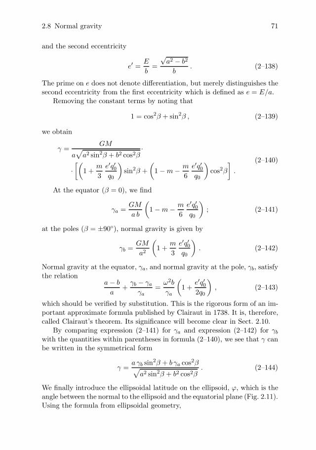
We finally introduce the ellipsoidal latitude on the ellipsoid, ϕ, which is theangle between the normal to the ellipsoid and the equatorial plane (Fig. 2.11).Using the formula from ellipsoidal geometry,


Oa

b

N

''¯

P

Fig. 2.11. Ellipsoidal latitude ϕ, geocentric latitude ϕ, reduced(ellipsoidal-harmonic) latitude β for a point P on the ellipsoid

tan β =b

atan ϕ , (2–145)

we obtain

γ =a γa cos2ϕ + b γb sin2ϕ√

a2 cos2ϕ + b2 sin2ϕ. (2–146)

The computation is left as an exercise for the reader. This rigorous formulafor normal gravity on the ellipsoid is due to Somigliana from 1929.

We close this section with a short remark on the vertical gradient ofgravity at the reference ellipsoid, ∂γ/∂su = ∂γ/∂h. Bruns’ formula (2–40),applied to the normal gravity field with the corresponding ellipsoidal heighth and with � = 0, yields

∂γ

∂h= −2γ J − 2ω2 . (2–147)

The mean curvature of the ellipsoid is given by

J =12

(1M

+1N

), (2–148)

where M and N are the principal radii of curvature: M is the radius in thedirection of the meridian, and N is the normal radius of curvature, takenin the direction of the prime vertical. From ellipsoidal geometry, we use theformulas

M =c

(1 + e′2 cos2ϕ)3/2, N =

c

(1 + e′2 cos2ϕ)1/2, (2–149)

2.9 Expansion of the normal potential in spherical harmonics 73

where

c =a2

b(2–150)

is the radius of curvature at the pole. The normal radius of curvature, N ,admits a simple geometrical interpretation (Fig. 2.11). It is, therefore, alsoknown as the “normal terminated by the minor axis” (Bomford 1962: p. 497).

2.9 Expansion of the normal potential in sphericalharmonics

We have found the gravitational potential of the normal figure of the earthin terms of ellipsoidal harmonics in (2–124) as

V =GM

Etan−1 E

u+

13

ω2a2 q

q0P2(sin β) . (2–151)

Now we wish to express this equation in terms of spherical coordinatesr, ϑ, λ.

We first establish a relation between ellipsoidal-harmonic and sphericalcoordinates. By comparing the rectangular coordinates in these two systemsaccording to Eqs. (1–26) and (1–151), we get

r sin ϑ cos λ =√

u2 + E2 cos β cos λ ,

r sin ϑ sinλ =√

u2 + E2 cos β sin λ ,

r cos ϑ = u sin β .

(2–152)

The longitude λ is the same in both systems. We easily find from theseequations

cot ϑ =u√

u2 + E2tan β ,

r =√

u2 + E2 cos2β .

(2–153)

The direct transformation of (2–151) by expressing u and β in terms ofr and ϑ by means of equations (2–153) is extremely laborious. However, theproblem can be solved easily in an indirect way.

We expand tan−1(E/u) into the well-known power series

tan−1 E

u=

E

u− 1

3

(E

u

)3

+15

(E

u

)5

− . . . . (2–154)

The substitution of this series into the first equation of formula (2–113), i.e.,

q =12

[(1 + 3

u2

E2

)tan−1 E

u− 3

u

E

], (2–155)


leads, after simple manipulations, to

q = 2

[1

3 · 5(

E

u

)3

− 25 · 7

(E

u

)5

+3

7 · 9(

E

u

)7

− . . .

]. (2–156)

More concisely, we have

tan−1 E

u=

E

u+

∞∑n=1

(−1)n1

2n + 1

(E

u

)2n+1

,

q = −∞∑

n=1

(−1)n2n

(2n + 1)(2n + 3)

(E

u

)2n+1

.

(2–157)

By inserting these relations into (2–151) we obtain

V =GM

u+

GM

E

∞∑n=1

(−1)n1

2n + 1

(E

u

)2n+1

− ω2a2

3q0

∞∑n=1

(−1)n2n

(2n + 1)(2n + 3)

(E

u

)2n+1

P2(sin β) .

(2–158)

Introducing m, defined by (2–137), and the second eccentricity e′ = E/b, wefind

V =GM

u+

∞∑n=1

(−1)nGM

(2n + 1)E

(E

u

)2n+1

·

·[1 − m e′

3q0

2n2n + 3

P2(sin β)]

. (2–159)

We expand the potential V into a series of spherical harmonics. Becauseof the rotational symmetry, there will be only zonal terms, and because ofthe symmetry with respect to the equatorial plane, there will be only evenzonal harmonics. The zonal harmonics of odd degree change sign for negativelatitudes and must, therefore, be absent. Accordingly, the series has the form

V =GM

r+ A2

P2(cos ϑ)r3

+ A4P4(cos ϑ)

r5+ · · · . (2–160)

We next have to determine the coefficients A2, A4, . . . . For this purpose, weconsider a point on the axis of rotation, outside the ellipsoid. For this point,we have β = 90◦, ϑ = 0◦, and, by (2–153), u = r. Then (2–159) becomes

V =GM

r+

∞∑n=1

(−1)nGM E2n

2n + 1

(1 − 2n

2n + 3m e′

3q0

)1

r2n+1, (2–161)

2.9 Expansion of the normal potential in spherical harmonics 75

and (2–160) takes the form

V =GM

r+

A2

r3+

A4

r5+ · · · =

GM

r+

∞∑n=1

A2n1

r2n+1. (2–162)

Here we have used the fact that for all values of n

Pn(1) = 1 (2–163)

(see also Fig. 1.4). Comparing the coefficients in both expressions for V , wefind

A2n = (−1)nGM E2n

2n + 1

(1 − 2n

2n + 3m e′

3q0

). (2–164)

Equations (2–160) and (2–164) give the desired expression for the potentialof the level ellipsoid as a series of spherical harmonics.

The second-degree coefficient A2 is

A2 = G (A − C) . (2–165)

This follows from (2–91) by using A = B for reasons of symmetry. The Cis the moment of inertia with respect to the axis of rotation, and A is themoment of inertia with respect to any axis in the equatorial plane. By lettingn = 1 in (2–164), we obtain

A2 = −13

GM E2

(1 − 2

15m e′

q0

). (2–166)

Comparing this with the preceding Eq. (2–165), we find

G (C − A) =13

GM E2

(1 − 2

15m e′

q0

). (2–167)

Thus, the difference between the principal moments of inertia is expressedin terms of “Stokes’ constants” a, b, M , and ω.

It is possible to eliminate q0 from Eqs. (2–164) and (2–167), obtaining

A2n = (−1)n3GM E2n

(2n + 1)(2n + 3)

(1 − n + 5n

C − A

M E2

). (2–168)

If we write the potential V in the form

V =GM

r

[1 + C2

(a

r

)2P2(cos ϑ) + C4

(a

r

)4P4(cos ϑ) + · · ·

]

=GM

r

[1 +

∞∑n=1

C2n

(a

r

)2nP2n(cos ϑ)

],

(2–169)


then the C2n are given by

C2n = −J2n = (−1)n3e2n

(2n + 1)(2n + 3)

(1 − n + 5n

C − A

M E2

). (2–170)

Here we have introduced the first eccentricity e = E/a. For n = 1 this givesthe important formula

C20 = −C − A

M a2(2–171)

or, equivalently,

J2 =C − A

M a2, (2–172)

which is in agreement with the respective relation in (2–95) when taking intoaccount the rotational symmetry causing A = B.

Finally, we note that on eliminating q0 = (1/i)Q2(i(b/E)) by usingEq. (2–167), and U0 by using Eq. (2–122), we may write the expansion of Vin ellipsoidal harmonics, Eq. (2–110), in the form

V (u, β) =i

EGM Q0

(i

u

E

)+

15i2E3

G(C − A − 1

3 M E2)Q2

(i

u

E

)P2(sin β) .

(2–173)

This shows that the coefficients of the ellipsoidal harmonics of degrees zeroand two are functions of the mass and of the difference between the twoprincipal moments of inertia. The analogy to the corresponding spherical-harmonic coefficients (2–91) is obvious. This is a closed formula, not a trun-cated series!

2.10 Series expansions for the normal gravity field

Since the earth ellipsoid is very nearly a sphere, the quantities

E =√

a2 − b2 , linear eccentricity,

e =E

a, first (numerical) eccentricity,

e′ =E

b, second (numerical) eccentricity,

f =a − b

a, flattening,

(2–174)

2.10 Series expansions for the normal gravity field 77

and similar parameters that characterize the deviation from a sphere aresmall. Therefore, series expansions in terms of these or similar parameterswill be convenient for numerical calculations.

Linear approximationIn order that the readers may find their way through the subsequent practicalformulas, we first consider an approximation that is linear in the flattening f .Here we get particularly simple and symmetrical formulas which also exhibitplainly the structure of the higher-order expansions.

It is well known that the radius vector r of an ellipsoid is approximatelygiven by

r = a (1 − f sin2ϕ) . (2–175)

As we will see subsequently, normal gravity may, to the same approximation,be written

γ = γa (1 + f∗ sin2ϕ) . (2–176)

For ϕ = ±90◦, at the poles, we have r = b and γ = γb. Hence, we may write

b = a (1 − f) , γb = γa (1 + f∗) , (2–177)

and solving for f and f∗, we obtain

f =a − b

a,

f∗ =γb − γa

γa,

(2–178)

so that f is the flattening defined by (2–174), and f∗ is an analogous quantitywhich may be called gravity flattening.

To the same approximation, (2–143) becomes

f + f∗ = 52 m , (2–179)

where

m.=

ω2a

γa=

centrifugal force at equatorgravity at equator

. (2–180)

This is Clairaut’s theorem in its original form. It is one of the most strikingformulas of physical geodesy: the (geometrical) flattening f in (2–178) canbe derived from f∗ and m, which are purely dynamical quantities obtainedby gravity measurements; that is, the flattening of the earth can be obtainedfrom gravity measurements.

Clairaut’s formula is only a first approximation and must be improved,first by the inclusion of higher-order ellipsoidal terms in f , and secondly bytaking into account the deviation of the earth’s gravity field from the normalgravity field. But the principle remains the same.


Second-order expansion

We now expand the closed formulas of the two preceding sections into seriesin terms of the second numerical eccentricity e′ and the flattening f , ingeneral up to and including e′4 or f2. Terms of the order of e′6 or f3 andhigher will usually be neglected.

We start from the series

tan−1 E

u=

E

u− 1

3

(E

u

)3

+15

(E

u

)5

− 17

(E

u

)7

+ · · · ,

q = 2

[1

3 · 5(

E

u

)3

− 25 · 7

(E

u

)5

+3

7 · 9(

E

u

)7

− · · ·]

,

q′ = 6

[1

3 · 5(

E

u

)3

− 15 · 7

(E

u

)5

+1

7 · 9(

E

u

)7

− · · ·]

.

(2–181)

The first two series have already been used in the preceding section in (2–154) and (2–156), respectively; the third is obtained by substituting thetan−1 series into the closed formula (2–133) for q′.

On the reference ellipsoid S0, we have u = b and

E

u=

E

b= e′ , (2–182)

so that

tan−1e′ = e′ − 13 e′3 + 1

5 e′5 · · · ,

q0 = 215 e′3

(1 − 6

7 e′2 · · · ) ,

q′0 = 25 e′2

(1 − 3

7 e′2 · · · ) ,

e′ q′0q0

= 3(1 + 3

7 e′2 · · · ) .

(2–183)

We also need the series

b =a√

1 + e′2= a

(1 − 1

2 e′2 + 38 e′4 · · · ) . (2–184)


Potential and gravityBy substituting these expressions into the closed formulas (2–123), (2–141),(2–142), and (2–143), we obtain, up to and including the order e′4, the fol-lowing relations.Potential:

U0 =GM

b

(1 − 1

3 e′2 + 15 e′4

)+ 1

3 ω2a2 . (2–185)

Gravity at the equator and the pole:

γa =GM

ab

(1 − 3

2 m − 314 e′2m

),

γb =GM

a2

(1 + m + 3

7 e′2m).

(2–186)

Clairaut’s theorem:

f + f∗ =52

ω2b

γa

(1 +

935

e′2)

. (2–187)

The ratio ω2a/γa may be expressed as

ω2a

γa= m + 3

2 m2 , (2–188)

which is a more accurate version of (2–180).From the first equation of (2–186), we find

GM = a b γa

(1 + 3

2 m + 314 e′2m + 9

4 m2), (2–189)

which gives the mass in terms of equatorial gravity. Using this equation, wecan express GM in Eq. (2–185) in terms of γa, obtaining

U0 = a γa

(1 − 1

3 e′2 + 116 m + 1

5 e′4 − 27 e′2m + 11

4 m2). (2–190)

Here we have eliminated ω2a by replacing it with GM m/b.Now we can turn to Eq. (2–146) for normal gravity. A simple manipula-

tion yields

γ = γa

1 + b γb−a γa

a γbsin2ϕ√

1 − a2−b2

a2 sin2ϕ. (2–191)

The denominator is expanded into a binomial series:

1√1 − x

= 1 + 12 x + 3

8 x2 + · · · . (2–192)


Then the abbreviated series

a2 − b2

a2=

e′2

1 + e′2= e′2 − e′4 ,

b γb − a γa

a γa= −e′2 + 5

2 m2 + e′4 − 137 e′2m + 15

4 m2

(2–193)

are introduced and we obtain, upon substitution,

γ = γa

[1 +

(− 12 e′2 + 5

2 m + 12 e′4 − 13

7 e′2m + 154 m2

)sin2 ϕ

+(− 1

8 e′4 + 54 e′2m

)sin4ϕ

].

(2–194)

We may also express these quantities in terms of the flattening f by substi-tuting the equation

e′2 =1

(1 − f)2− 1 = 2f + 3f2 + · · · . (2–195)

The flattening f is most commonly used; it offers a slight advantage overthe second eccentricity e′ in that it is of the same order of magnitude as m:it is not immediately apparent that m2, e′2m, and e′4 are quantities of thesame order of magnitude. We obtain

GM = a b γa

(1 + 3

2 m + 37 f m + +9

4 m2), (2–196)

U0 = a γa

(1 − 2

3 f + 116 m − 1

5 f2 − 47 f m + 11

4 m2), (2–197)

γ = γa

[1 +

(− f + 52 m + 1

2 f2 − 267 f m + 15

4 m2)

sin2ϕ

+(− 1

2 f2 + 52 f m

)sin4ϕ

].

(2–198)

The last formula is usually abbreviated as

γ = γa (1 + f2 sin2ϕ + f4 sin4ϕ) , (2–199)

so that we have

f2 = −f + 52 m + 1

2 f2 − 267 f m + 15

4 m2 ,

f4 = −12 f2 + 5

2 f m .

(2–200)

By substitutingsin4ϕ = sin2ϕ − 1

4 sin2 2ϕ , (2–201)


we finally obtain

γ = γa (1 + f∗ sin2ϕ − 14 f4 sin2 2ϕ) , (2–202)

wheref∗ =

γb − γa

γa= f2 + f4 (2–203)

is the “gravity flattening”.

Coefficients of spherical harmonicsEquation (2–167) for the principal moments of inertia yields at once

C − A

M E2=

13− 2

45m e′

q0. (2–204)

Expanding q0 by means of (2–183), we find

C − A

M E2=

1e′2(

13 e′2 − 1

3 m − 27 e′2m

). (2–205)

Substituting this into (2–170) yields

−C20 = J2 =C − A

M E2= 1

3 e′2 − 13 m − 1

3 e′4 + 121 e′2m

= 23 f − 1

3 m − 13 f2 + 2

21 f m ,

(2–206)

−C40 = J4 = −15 e′4 + 2

7 e′2m = −45 f2 + 4

7 f m . (2–207)

The higher C or J , respectively, are already of an order of magnitude thatwe have neglected.

Gravity above the ellipsoidDenoting the height above the ellipsoid as ellipsoidal height h, then, in caseof a small height, the normal gravity γh at this height can be expanded intoa series in terms of h:

γh = γ +∂γ

∂hh +

12

∂2γ

∂h2h2 + · · · , (2–208)

where γ and its derivatives are referred to the ellipsoid, where h = 0.The first derivative ∂γ/∂h may be obtained by applying Bruns’ formula

(2–147) together with (2–148) to the ellipsoidal height h (instead of H):

∂γ

∂h= −γ

(1M

+1N

)− 2ω2 , (2–209)


where M, N are the principal radii of curvature of the ellipsoid, defined by(2–149). Since

1M

=b

a2

(1 + e′2 cos2ϕ

)3/2 =b

a2

(1 + 3

2 e′2 cos2ϕ · · · ) ,

1N

=b

a2

(1 + e′2 cos2ϕ

)1/2 =b

a2

(1 + 1

2 e′2 cos2ϕ · · · ) ,

(2–210)

we have

1M

+1N

=b

a2

(2 + 2e′2 cos2ϕ

)=

2ba2

(1 + 2f cos2ϕ) . (2–211)

Here we have limited ourselves to terms linear in f , since the elevation h isalready a small quantity. Thus, we find from (2–209) after simple manipula-tions:

∂γ

∂h= −2γ

a(1 + f + m − 2f sin2ϕ) . (2–212)

The second derivative ∂2γ/∂h2 may be taken from the spherical approxima-tion, obtained by neglecting e′2 or f :

γ =GM

a2,

∂γ

∂h=

∂γ

∂a= −2GM

a3,

∂2γ

∂h2=

∂2γ

∂a2=

6GM

a4, (2–213)

so that∂2γ

∂h2=

6γa2

. (2–214)

Thus we obtain

γh = γ

[1 − 2

a(1 + f + m − 2f sin2ϕ)h +

3a2

h2

]. (2–215)

Using Eq. (2–198) for γ, we may also write the difference γh − γ in the form

γh − γ = −2γa

a

[1 + f + m +

(− 3f + 52 m

)sin2ϕ)

]h +

3γa

a2h2 . (2–216)

The symbol γh denotes the normal gravity for a point at latitude ϕ, situatedat height h above the ellipsoid; γ is the gravity at the ellipsoid itself, for thesame latitude ϕ, as given by (2–202) or equivalent formulas.

Second-order series developments for the inner gravity field are found inMoritz (1990: Chap. 4); this is the main reason for such a development here,because today one uses the closed formulas wherever possible.

2.11 Reference ellipsoid – numerical values 83

2.11 Reference ellipsoid – numerical values

Some historyThe reference ellipsoid and its gravity field are completely determined by fourconstants. Before the satellite era, one took the following four parameters:

a . . . semimajor axis ,f . . . flattening ,

γa . . . equatorial gravity ,ω . . . angular velocity .

(2–217)

The values best known and most widely used have been those of the Inter-national Ellipsoid:

a = 6378 388.000 m ,f = 1/297.000 ,

γa = 978.049 000 gal ,ω = 0.729 211 51 · 10−4 s−1 .

(2–218)

The geometric parameters a and f were determined by Hayford in 1909 fromisostatically reduced astrogeodetic data in the United States. They wereadopted for the International Ellipsoid by the assembly of the InternationalAssociation of Geodesy (IAG) at Madrid in 1924. The equatorial gravityvalue γa was computed by Heiskanen (1924, 1928) from isostatically reducedgravity data. The corresponding international gravity formula,

γ = 978.0490 (1 + 0.005 2884 sin2ϕ − 0.000 0059 sin2 2ϕ) gal , (2–219)

was adopted by the assembly of IAG at Stockholm in 1930; whose coefficientswere computed from the assumed values for a, f, γa, ω by Cassinis (1930)using Eqs. (2–200), (2–202), (2–203).

All parameters of the International Ellipsoid and its gravity field canbe computed from (2–218) to any desired degree of accuracy, which merelyexpresses the inner consistency. In this way, we find (rounded values)

b = 6356 912 m ,E = 522 976 m ,e′2 = 0.006 7682 ,m = 0.003 4499 .

(2–220)

For the constants in the spherical-harmonic expansion of the normalgravity field, we find the values

−C20 = J2 =C − A

M a2= 0.001 0920 ,

−C40 = J4 = −0.000 002 43 .

(2–221)


The change of normal gravity with elevation is given by the formula(2–216), which for the International Ellipsoid becomes

γh = γ − (0.308 77 − 0.000 45 sin2ϕ)h + 0.000 072h2 , (2–222)

where γh and γ are measured in gal, and h is the elevation in kilometer.Although the International Ellipsoid can no longer be considered the

closest approximation of the earth by an ellipsoid, it may still be used asa reference ellipsoid for geodetic purposes. An official change of a referencesystem must be very carefully considered because a large amount of datamay be referred to such a system.

The eastern countries have used the ellipsoid of Krassowsky:

a = 6378 245 m ,f = 1/298.3 .

(2–223)

Contemporary dataAfter the start of Sputnik, the first artificial satellite, in 1957, the Interna-tional Astronomical Union, in 1964, adopted a new set of constants, amongthem a = 6378 160 m and f = 1/298.25. The value of a, which is consid-erably smaller than that for the International Ellipsoid, incorporates astro-geodetic determinations; the change in the value of J2, and consequently off , is due to the results from artificial satellites.

In 1967, these values were taken by the International Union of Geodesyand Geophysics (IUGG) as the Geodetic Reference System 1967.

This decision was soon seen to be wrong; especially the value of a wasrecognized to be too large: now we believe to be on the order of 6 378 137 m,the value of the Geodetic Reference System 1980 (GRS 1980) and, based onit, the World Geodetic System 1984 (WGS 84). More details of these twosystems are given below.

Geodetic Reference System 1980 (GRS 1980)The GRS 1980 has been adopted at the XVII General Assembly of the IUGGin Canberra, December 1979, by Resolution No. 7. Inherently, this resolu-tion recognizing that the Geodetic Reference System 1967 adopted at theXIV General Assembly of IUGG, Lucerne, 1967, no longer represents thesize, shape, and gravity field of the earth to an accuracy adequate for manygeodetic, geophysical, astronomical, and hydrographic applications and con-sidering that more appropriate values are now available, recommends thatthe Geodetic Reference System 1967 be replaced by the new Geodetic Refer-ence System 1980 which is also based on the theory of the geocentric equipo-tential ellipsoid. The four defining parameters of the GRS 1980 are given in


Table 2.1. Defining parameters of the GRS 1980

Parameter and value Descriptiona = 6378 137 m semimajor axis of the ellipsoidGM = 3986 005 · 108 m3 s−2 geocentric gravitational constant of the

earth (including the atmosphere)J2 = 108 263 · 10−8 dynamical form factor of the earth (ex-

cluding the permanent tidal deforma-tion)

ω = 7292 115 · 10−11 rad s−1 angular velocity of the earth

Table 2.1. Note that these parameters, as given in the table, are definedas exact! Note also that GM , the “geocentric gravitational constant” of theearth, may also more figuratively be denoted as “product of the (Newtonian)gravitational constant and the earth’s mass”.

On the basis of these defining parameters and by the computationalformulas given in Moritz (1980 b), the geometrical and physical constants ofTable 2.2 may be derived.

The GRS 1980 is still (2005) valid as the official reference system of theIUGG and it forms the fundamental basis of the WGS 84.

World Geodetic System 1984 (WGS 84)As just mentioned, the WGS 84 may be regarded as a descendant of theGRS 1980. Due to its still increasing importance, we consider it appropriateto describe the WGS 84 in some more detail.

Following the National Imagery and Mapping Agency (2000) of the USA,the definition of the WGS 84 may be described in the following way. TheWGS 84 is a Conventional Terrestrial Reference System (CTRS). The def-inition of this coordinate system follows the criteria as outlined by the In-ternational Earth Rotation Service (IERS). The criteria for this system arethe following:

• it is geocentric, the center of mass being defined for the whole earthincluding oceans and atmosphere;

• its scale is that of the local earth frame, in the meaning of a relativistictheory of gravitation;

• its orientation was initially given by the Bureau International de l’Heure(BIH) orientation of 1984.0;

• its time evolution in orientation will create no residual global rotationwith regards to the crust.


Table 2.2. GRS 1980 derived constants

Parameter and value Description

Geometrical constants

b = 6356 752.3141 m semiminor axis of the ellipsoidE = 521 854.0097 m linear eccentricityc = 6399 593.6259 m polar radius of curvaturee2 = 0.006 694 380 022 90 first eccentricity squarede′2 = 0.006 739 496 775 48 second eccentricity squaredf = 0.003 352 810 681 18 flattening1/f = 298.257 222 101 reciprocal flattening

Physical constants

U0 = 62636 860.850 m2 s−2 normal potential at the ellipsoidJ4 = −0.000 002 370 912 22 spherical-harmonic coefficientJ6 = 0.000 000 006 083 47 spherical-harmonic coefficientJ8 = −0.000 000 000 014 27 spherical-harmonic coefficientm = 0.003 449 786 003 08 m = ω2a2b/(GM)γa = 9.780 326 7715 m s−2 normal gravity at the equatorγb = 9.832 186 3685 m s−2 normal gravity at the pole

The WGS 84 is a right-handed, earth-fixed orthogonal coordinate system.The origin and axes are defined in the following way:

• Origin: earth’s center of mass.• Z-axis: the direction of the IERS Reference Pole (IRP); this direction

corresponds to the direction of the BIH Conventional Terrestrial Pole(CTP) (epoch 1984.0). In other terms, the Z-axis is, by convention,identical to the mean position of the earth’s rotational axis.

• X-axis: intersection of the IERS Reference Meridian (IRM) and theplane passing through the origin and normal to the Z-axis; the IRM iscoincident with the BIH Zero Meridian (epoch 1984.0); in other terms,the X-axis is associated with the mean Greenwich meridian.

• Y -axis: this axis completes a right-handed, earth-centered-earth-fixed(ECEF) orthogonal coordinate system.

The WGS 84 origin also serves as the geometric center of the WGS 84 ellip-soid and the Z-axis serves as the rotational axis of this ellipsoid of revolution.

This completes the definition of the WGS 84 as given in National Imageryand Mapping Agency (2000). Note that the definition of the WGS 84 CTRShas not changed in any fundamental way.


Reference frames: WGS 84 and ITRFNow we need the distinction between definition and realization. When usingthe term “coordinate system” or “reference system”, then this implies thedefinition only; however, when using the term “coordinate frame”, then arealization is implied (Mueller 1985). So far, we have only given a definitionof the WGS 84; therefore, we ought to denote this as WGS 84 CTRS. Nowwe consider a realization and, therefore, use the term “coordinate frame”.

Following closely National Imagery and Mapping Agency (2000) andHofmann-Wellenhof et al. (2001: Sect. 3.2.1), an example of a terrestrialreference frame is – on the basis of the previous definition – the WGS 84reference frame (often simply denoted as WGS 84 – as we will also do).Associated to this frame is a geocentric ellipsoid of revolution, originally de-fined by the four parameters (1) semimajor axis a, (2) normalized seconddegree zonal gravitational coefficient C20, (3) truncated angular velocity ofthe earth ω, and (4) earth’s gravitational constant G. This frame has beenused for GPS since 1987.

Another example for a terrestrial reference frame is the one producedby the IERS and is called International Terrestrial Reference Frame (ITRF)(McCarthy 1996). The definition of the axes is analogous to the WGS 84, i.e.,the Z-axis is defined by the IERS Reference Pole (IRP) and the X-axis liesin the IERS Reference Meridian (IRM); however, the realization differs! TheITRF is realized by a number of terrestrial sites where temporal effects (platetectonics, tidal effects) are also taken into account. Thus, ITRF is regularlyupdated (almost every year) and the acronym is supplemented by the lasttwo digits of the last year whose data were used in the formation of theframe, e.g., ITRF89, ITRF90, ITRF91, ITRF92, ITRF93, ITRF94, ITRF95,ITRF96, ITRF97, or the full designation of the year, e.g., ITRF2000.

The comparison of the original WGS 84 and ITRF revealed remarkabledifferences (Malys and Slater 1994):

1. The WGS 84 was established through Doppler observations from theTRANSIT satellite system, while ITRF is based on Satellite LaserRanging (SLR) and Very Long Baseline Interferometry (VLBI) obser-vations. The accuracy of the TRANSIT reference stations was esti-mated to be in the range of 1 to 2 meters, while the accuracy of theITRF reference stations is at the centimeter level.

2. The numerical values for the original defining parameters differ fromthose in the ITRF. The only significant difference, however, was inthe earth’s gravitational constant GWGS −GITRF = 0.582 · 108 m3 s−2,which resulted in measurable differences in the satellite orbits.

On the basis of this information, the former U.S. Defense Mapping Agency


(DMA) has proposed to replace the value of G in the WGS 84 by the standardIERS value and to refine the coordinates of the GPS tracking stations. Therevised WGS 84, valid since January 2, 1994, has been given the designationWGS 84 (G 730), where the ‘G’ indicates that the respective coordinatesused were obtained through GPS and the following number 730 indicatesthe GPS week number when DMA has implemented the refined system.

In 1996, the U.S.National Imagery and Mapping Agency (NIMA) – thesuccessor of DMA – has implemented a revised version of the frame denotedas WGS 84 (G 873) and being valid since September 29, 1996. The frame isrealized by monitor stations with refined coordinates. The associated ellip-soid and its gravity field are now defined by the four parameters a, f,GM,ω,which are slightly different compared to the respective ITRF values, e.g., thecurrent WGS 84 (G 873) frame and the ITRF97 show insignificant systematicdifferences of less than 2 cm. Hence, they are virtually identical.

Note that the refinements applied to the WGS 84 reference frame havereduced the uncertainties in the coordinates of the frame, the uncertaintyof the gravitational model, and the uncertainty of the geoid undulations;however, they have not changed the WGS 84 coordinate system in the senseof definition !

More general, the relationship between the WGS 84 and the ITRF ischaracterized by two statements: (1) WGS 84 and ITRF are consistent; (2)the differences between WGS 84 and ITRF are in the centimeter range world-wide (National Imagery and Mapping Agency 2000).

However, if a transformation between reference frames is required, thisis accomplished by a datum transformation (see Sect. 5.7).

Numerical values for the WGS 84 (reference frame)As mentioned at the very beginning of Sect. 2.11, the reference ellipsoid andits gravity field are completely determined by four constants. The currentdefining parameters for WGS 84 are listed in Table 2.3.

Table 2.3. Defining parameters of the WGS 84

Parameter and value Descriptiona = 6378 137 m semimajor axis of the ellipsoidf = 1/298.257 223 563 flattening of the ellipsoidGM = 3986 004.418 · 108 m3 s−2 geocentric gravitational constant of

the earth (including the atmosphere)ω = 7292 115 · 10−11 rad s−1 angular velocity of the earth


Table 2.4. WGS 84 reference ellipsoid derived constants

Parameter and value Description

Geometrical constants

C20 = −0.484 166 774 985 · 10−3 normalized second-degree harmonicb = 6356 752.3142 m semiminor axis of the ellipsoide = 8.181 919 084 2622 · 10−2 first eccentricitye2 = 6.694 379 990 14 · 10−3 first eccentricity squarede′ = 8.209 443 794 9696 · 10−2 second eccentricitye′2 = 6.739 496 742 28 · 10−3 second eccentricity squaredE = 5.218 540 084 2339 · 105 linear eccentricityc = 6399 593.6258 m polar radius of curvature

b/a = 0.996 647 189 335 axis ratio

Physical constants

U0 = 62636 851.7146 m2 s−2 normal potential at the ellipsoidγa = 9.780 325 3359 m s−2 normal gravity at the equatorγb = 9.832 184 9378 m s−2 normal gravity at the poleγ = 9.797 643 2222 m s−2 mean value of normal gravityM = 5.973 3328 · 1024 kg mass of the earth (includes atmosphere)m = 0.003 449 786 506 84 m = ω2a2b/(GM)

Some history (even if only some years old) is important here becausethe parameters selected to originally define the WGS 84 reference ellipsoidwere the semimajor axis a, the product of the earth’s mass and the grav-itational constant GM (also denoted as “geocentric gravitational constantof the earth”), the normalized second-degree zonal gravitational coefficientC20, and the earth’s angular velocity ω. Due to significant refinements ofthese original defining parameters, the DMA recommended, e.g., a refinedvalue for the GM parameter.

Anyway, a decision was made to retain the original WGS 84 referenceellipsoid values for the semimajor axis a = 6378 137 m and for the flatteningf = 1/298.257 223 563. For this reason, the four defining parameters werechosen to be a, f,GM,ω.

Readers who like some confusion may continue right here; otherwise skipthis short paragraph. Due to this new choice of the defining parameters,there are in addition two distinct values for the C20 term, one is dynami-cally derived and the other geometrically by the defining parameters. The


geometric derivation based on the four defining parameters a, f,GM,ω yieldsC20 = −0.484 166 774 985 · 10−3 which differs from the original value by7.5015 · 10−11. For many more details refer to National Imagery and Map-ping Agency (2000).

We conclude these considerations by a useful table. Using the four defin-ing parameters, it is possible to derive the more commonly used geometricconstants and physical constants (Table 2.4) associated with the WGS 84reference ellipsoid.

Numerical comparison of GRS 1980 and WGS 84As mentioned previously, the GRS 1980 is the basis of the WGS 84. However,due to different defining parameters on the one hand and, e.g., a refined valuefor GM for the WGS 84 on the other hand, numerical differences betweenthe GRS 1980 and the WGS 84 arise. Some of these differences are given inTable 2.5.

Table 2.5. Numerical comparison between GRS 1980 and WGS 84

Parameter GRS 1980 WGS 84

GM 3 986 005 · 108 m3 s−2 3 986 004.418 · 108 m3 s−2

1/f 298.257 222 101 298.257 223 563b 6 356 752.3141 m 6356 752.3142 me2 0.006 694 380 022 90 0.006 694 379 990 14e′2 0.006 739 496 775 48 0.006 739 496 742 28E 521 854.0097 m 521 854.0084 mc 6 399 593.6259 m 6399 593.6258 mU0 62 636 860.850 m2 s−2 62 636 851.7146 m2 s−2

γa 9.780 326 7715 m s−2 9.780 325 3359 m s−2

γb 9.832 186 3685 m s−2 9.832 184 9378 m s−2

m 0.003 449 786 003 08 0.003 449 786 506 84

2.12 Anomalous gravity field, geoidal undulations,and deflections of the vertical

The small difference between the actual gravity potential W and the normalgravity potential U is denoted by T , so that

W (x, y, z) = U(x, y, z) + T (x, y, z) ; (2–224)

2.12 Anomalous gravity field 91

P

n'

°°Q°

gP

n

Q

geoid

W W= 0

referenceellipsoid

U W= 0

N

Fig. 2.12. Geoid and reference ellipsoid

T is called the anomalous potential, or disturbing potential. We compare thegeoid

W (x, y, z) = W0 (2–225)

with a reference ellipsoidU(x, y, z) = W0 (2–226)

of the same potential U0 = W0. A point P of the geoid is projected ontothe point Q of the ellipsoid by means of the ellipsoidal normal (Fig. 2.12).The distance PQ between geoid and ellipsoid is called the geoidal height, orgeoidal undulation, and is denoted by N . Unfortunately, there is a conflict ofnotation here. Denoting both the normal radius of curvature of the ellipsoidand the geoidal height by N is well established in geodetic literature. Wecontinue this practice, as there is little chance of confusion.

Consider now the gravity vector g at P and the normal gravity vector γat Q. The gravity anomaly vector ∆g is defined as their difference:

∆g = gP − γQ . (2–227)

A vector is characterized by magnitude and direction. The difference in mag-nitude is the gravity anomaly

∆g = gP − γQ ; (2–228)

the difference in direction is the deflection of the vertical.The deflection of the vertical has two components, a north-south com-

ponent ξ and an east-west component η (Fig. 2.13). As the direction of thevertical is directly defined by the astronomical coordinates latitude Φ andlongitude Λ, the components ξ and η can be expressed by them in a sim-ple way. The actual astronomical coordinates of the geoidal point P , which


||z

Gre

enw

ich

mer

idia

n�

¸

�

P'

´

»

ellip

soid

alno

rmal

plu

mb

line

�–¸

cos'

�–¸

nn'

Fig. 2.13. The deflection of the vertical as illustrated by means of aunit sphere with center at P

define the direction of the plumb line n or of the gravity vector g, can bedetermined by astronomical measurements. The ellipsoidal coordinates (orgeodetic coordinates in the sense of geographical coordinates on the ellip-soid) given by the direction of the ellipsoidal normal n′ have been denotedby ϕ and λ – these coordinates should not be confused with the ellipsoidal-harmonic coordinates of Sect. 1.15 ! It is evident that this λ is identical withthe geocentric longitude (and also with the ellipsoidal-harmonic longitude).Thus,

geoidal normal n, astronomical coordinates Φ, Λ ;

ellipsoidal normal n′, ellipsoidal coordinates ϕ, λ .(2–229)

From Fig. 2.13, we read

ξ = Φ − ϕ ,

η = (Λ − λ) cos ϕ .(2–230)

It is also possible to compare the vectors g and γ at the same point P . Thenwe get the gravity disturbance vector

δg = gP − γP . (2–231)


Accordingly, the difference in magnitude is the gravity disturbance

δg = gP − γP . (2–232)

The difference in direction – i.e., the deflection of the vertical – is the sameas before, since the directions of γP and γQ coincide virtually.

The gravity disturbance is conceptually even simpler than the gravityanomaly, but it has not been that important in terrestrial geodesy. Thesignificance of the gravity anomaly is that it is given directly: the gravityg is measured on the geoid (or reduced to it), see Chap. 3, and the normalgravity γ is computed for the ellipsoid.

A very important remarkSo far, for historical reasons, much more gravity anomalies ∆g are availableand are being processed than gravity disturbances δg. By GPS, however, thepoint P is determined rather than Q. Therefore, in future, we may expectthat δg will become more important than ∆g.

However, mirroring the present state of practice of physical geodesy, wecontinue mainly to work with ∆g. Most statements about ∆g will also applyfor δg, with obvious modifications, such as with Molodensky’s corrections(see Chap. 8), and Stokes’ formula will be replaced by Koch’s formula (seebelow in this chapter).

RelationsThere are several basic mathematical relations between the quantities justdefined. Since

UP = UQ +(

∂U

∂n

)Q

N = UQ − γ N , (2–233)

we haveWP = UP + TP = UQ − γ N + TP . (2–234)

BecauseWP = UQ = W0 , (2–235)

we findT = γ N (2–236)

(where we have omitted the subscript P on the left-hand side) or

N =T

γ. (2–237)

This is the famous Bruns formula, which relates the geoidal undulation tothe disturbing potential.


Next we consider the gravity disturbance. Since

g = grad W ,

γ = grad U ,(2–238)

the gravity disturbance vector (2–231) becomes

δg = grad (W − U) = grad T ≡[∂T

∂x,

∂T

∂y,

∂T

∂z

]. (2–239)

Theng = −∂W

∂n, γ = −∂U

∂n′.= −∂U

∂n, (2–240)

because the directions of the normals n and n′ almost coincide. Therefore,the gravity disturbance is given by

δg = gP − γP = −(

∂W

∂n− ∂U

∂n′

).= −

(∂W

∂n− ∂U

∂n

)(2–241)

orδg = −∂T

∂n. (2–242)

Since the elevation h is reckoned along the normal, we may also write

δg = −∂T

∂h. (2–243)

Comparing (2–242) with (2–239), we see that the gravity disturbance δg, be-sides being the difference in magnitude of the actual and the normal gravityvector, is also the normal component of the gravity disturbance vector δg.

We now turn to the gravity anomaly ∆g. Since

γP = γQ +∂γ

∂hN , (2–244)

we have−∂T

∂h= δg = gP − γP = gP − γQ − ∂γ

∂hN . (2–245)

Remembering the definition (2–228) of the gravity anomaly and taking intoaccount Bruns’ formula (2–237), we find the following equivalent relations:

−∂T

∂h= ∆g − ∂γ

∂hN , (2–246)

∆g = −∂T

∂h+

∂γ

∂hN , (2–247)


∆g = −∂T

∂h+

1γ

∂γ

∂hT , (2–248)

δg = ∆g − ∂γ

∂hN , (2–249)

δg = ∆g − 1γ

∂γ

∂hT , (2–250)

relating different quantities of the anomalous gravity field.Another equivalent form is

∂T

∂h− 1

γ

∂γ

∂hT + ∆g = 0 . (2–251)

This expression has been called the fundamental equation of physical geodesy,because it relates the measured quantity ∆g to the unknown anomalouspotential T . In future, the relation

∂T

∂h+ δg = 0 (2–252)

may replace it.It has the form of a partial differential equation. If ∆g were known

throughout space, then (2–251) could be discussed and solved as a real par-tial differential equation. However, since ∆g is known only along a surface(the geoid), the fundamental equation (2–251) can be used only as a bound-ary condition, which alone is not sufficient for computing T . Therefore, thename “differential equation of physical geodesy”, which is sometimes usedfor (2–251), is rather misleading.

One usually assumes that there are no masses outside the geoid. This isnot really true. But neither do we make observations directly on the geoid;we make them on the physical surface of the earth. In reducing the measuredgravity to the geoid, the effect of the masses outside the geoid is removed bycomputation, so that we can indeed assume that all masses are enclosed bythe geoid (see Chaps. 3 and 8).

In this case, since the density � is zero everywhere outside the geoid, theanomalous potential T is harmonic there and satisfies Laplace’s equation

∆T ≡ ∂2T

∂x2+

∂2T

∂y2+

∂2T

∂z2= 0 . (2–253)

This is a true partial differential equation and suffices, if supplemented bythe boundary condition (2–251), for determining T at every point outsidethe geoid. If we write the boundary condition in the form

−∂T

∂n+

1γ

∂γ

∂nT = ∆g , (2–254)


where ∆g is assumed to be known at every point of the geoid, then we see thata linear combination of T and ∂T/∂n is given upon that surface. Accordingto Sect. 1.13, the determination of T is, therefore, a third boundary-valueproblem of potential theory. If it is solved for T , then the geoidal height,which is the most important geometric quantity in physical geodesy, can becomputed by Bruns’ formula (2–237).

Therefore, we may say that the basic problem of physical geodesy, thedetermination of the geoid from gravity measurements, is essentially a thirdboundary-value problem of potential theory.

2.13 Spherical approximation and expansion of thedisturbing potential in spherical harmonics

The reference ellipsoid deviates from a sphere only by quantities of the orderof the flattening, f

.= 3 · 10−3. Therefore, if we treat the reference ellipsoidas a sphere in equations relating quantities of the anomalous field, this maycause a relative error of the same order. This error is usually permissible inN, T, ∆g, δg, etc. For instance, the absolute effect of this relative error onthe geoidal height is of the order of 3 ·10−3 N ; since N hardly exceeds 100 m,this error can usually be expected to be less than 1m.

As a spherical approximation, we have

γ =GM

r2,

∂γ

∂h=

∂γ

∂r= −2

GM

r3,

1γ

∂γ

∂h= −2

r. (2–255)

We introduce a mean radius R of the earth. It is often defined as the radius ofa sphere that has the same volume as the earth ellipsoid; from the condition

43 π R3 = 4

3 π a2 b , (2–256)

we getR = 3

√a2 b . (2–257)

In a similar way, we may define a mean value of gravity, γ0, as normal gravityat latitude ϕ = 45◦ (Moritz 1980b: p. 403). Numerical values of about

R = 6371 km, γ0 = 980.6 gal (2–258)

are usual. Then1γ

∂γ

∂h= − 2

R,

∂γ

∂h= −2γ0

R.

(2–259)

2.13 Spherical approximation 97

Since the normal to the sphere is the direction of the radius vector r, wehave to the same approximation

∂

∂n=

∂

∂h=

∂

∂r. (2–260)

In Bruns’ theorem (2–237) we may replace γ by γ0, and Eqs. (2–246)through (2–250) and (2–251) become

−∂T

∂h= ∆g +

2γ0

RN , (2–261)

∆g = −∂T

∂r− 2γ0

RN , (2–262)

∆g = −∂T

∂r− 2

RT , (2–263)

δg = ∆g +2γ0

RN , (2–264)

δg = ∆g +2R

T , (2–265)

∂T

∂r+

2R

T + ∆g = 0 . (2–266)

The last equation is the spherical approximation of the fundamental bound-ary condition.

RemarkThe meaning of this spherical approximation should be carefully kept inmind. It is used only in equations relating the small quantities T, N, ∆g, δg,etc. The reference surface is never a sphere in any geometrical sense, butalways an ellipsoid. As the flattening f is very small, the ellipsoidal formulascan be expanded into power series in terms of f , and then all terms containingf, f2, etc., are neglected. In this way one obtains formulas that are rigorouslyvalid for the sphere, but approximately valid for the actual reference ellipsoidas well. However, normal gravity γ in the gravity anomaly ∆g = g − γmust be computed for the ellipsoid to a high degree of accuracy. To speakof a “reference sphere” in space, in any geometric sense, may be highlymisleading.

Since the anomalous potential T = W −U is a harmonic function, it can beexpanded into a series of spherical harmonics:

T (r, ϑ, λ) =∞∑

n=0

(R

r

)n+1

Tn(ϑ, λ) . (2–267)


Tn(ϑ, λ) is Laplace’s surface harmonic of degree n. On the geoid, which as aspherical approximation corresponds to the sphere r = R, we have formally

T = T (R, ϑ, λ) =∞∑

n=0

Tn(ϑ, λ) . (2–268)

We need not be concerned with questions of convergence here. Differentiatingthe series (2–267) with respect to r, we find

δg = −∂T

∂r=

1r

∞∑n=0

(n + 1)(

R

r

)n+1

Tn(ϑ, λ) . (2–269)

On the geoid, where r = R, this becomes

δg = −∂T

∂r=

1R

∞∑n=0

(n + 1) Tn(ϑ, λ) . (2–270)

These series express the gravity disturbance in terms of spherical harmonics.The equivalent of (2–263) outside the earth is

∆g = −∂T

∂r− 2

rT . (2–271)

Its exact meaning will be discussed at the end of the following section. Thesubstitution of (2–269) and (2–267) into this equation yields

∆g =1r

∞∑n=0

(n − 1)(

R

r

)n+1

Tn(ϑ, λ) . (2–272)

On the geoid, this becomes

∆g =1R

∞∑n=0

(n − 1) Tn(ϑ, λ) . (2–273)

This is the spherical-harmonic expansion of the gravity anomaly.Note that even if the anomalous potential T contains a first-degree spher-

ical term T1(ϑ, λ), it will in the expression for ∆g be multiplied by the factor1−1 = 0, so that ∆g can never have a first-degree spherical harmonic – evenif T has one.

2.14 Gravity anomalies outside the earth 99

2.14 Gravity anomalies outside the earth

If a harmonic function H is given at the surface of the earth, then, as aspherical approximation, the values of H outside the earth can be computedby Poisson’s integral formula (1–123)

HP =R

4π

∫σ

∫r2 − R2

l3H dσ . (2–274)

The symbol∫∫

σ is the usual abbreviation for an integral extended over thewhole unit sphere. The meaning of the other notations is read from Fig. 2.14.The value of the harmonic function at the variable surface element R2 dσ isdenoted simply by H, whereas HP refers to the fixed point P . Then we get

l =√

r2 + R2 − 2R r cos ψ . (2–275)

The harmonic function H can be expanded into a series of spherical har-monics:

H =(

R

r

)H0 +

(R

r

)2

H1 +∞∑

n=2

(R

r

)n+1

Hn . (2–276)

By omitting the terms of degrees one and zero, we get a new function

H ′ = H −(

R

r

)H0 −

(R

r

)2

H1 =∞∑

n=2

(R

r

)n+1

Hn . (2–277)

P

terrestrial sphere

ÃÃ

Rd¾

R d2 ¾

unit sphere

r R=

r = 1

lr

Fig. 2.14. Notations for Poisson’s integral and derived formulas


The surface harmonics are given by

H0 =14π

∫σ

∫H dσ , H1 =

34π

∫σ

∫H cos ψ dσ (2–278)

according to equation (1–89). Hence, we find from (2–277), on expressing Hby Poisson’s integral (2–274) and substituting the integrals (2–278) for H0

and H1, the basic formula

H ′P =

14π

∫σ

∫ (r2 − R2

l3− 1

r− 3R

r2cos ψ

)H dσ . (2–279)

The reason for this modification of Poisson’s integral is that the formulasof physical geodesy are simpler if the functions involved do not contain har-monics of degrees zero and one. It is therefore convenient to split off theseterms. This is done automatically by the modified Poisson integral (2–279).

We now apply these formulas to the gravity anomalies outside the earth.Equation (2–272) yields at once

r ∆g =∞∑

n=0

(R

r

)n+1

(n − 1) Tn(ϑ, λ) . (2–280)

Just as Tn(ϑ, λ) is a Laplace surface harmonic, so is (n−1)Tn. Consequently,r ∆g, considered as a function in space, can be expanded into a series ofspherical harmonics and is, therefore, a harmonic function. Hence, we canapply Poisson’s formula to r ∆g, getting

r ∆gP =R

4π

∫σ

∫ (r2 − R2

l3− 1

r− 3R

r2cos ψ

)R ∆g dσ (2–281)

or

∆gP =R2

4π r

∫σ

∫ (r2 − R2

l3− 1

r− 3R

r2cos ψ

)∆g dσ . (2–282)

This is the formula for the computation of gravity anomalies outside theearth from surface gravity anomalies, or for the upward continuation of grav-ity anomalies.

Finally, we discuss the exact meaning of the gravity anomaly δgP outsidethe earth. We start with a convenient definition. The level surfaces of theactual gravity potential, the surfaces

W = constant , (2–283)

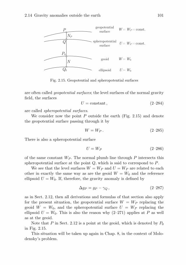
2.14 Gravity anomalies outside the earth 101

P

Q

geoid W W= 0

ellipsoid U W= 0

N

geopotentialsurface

spheropotentialsurface

W W= P = const.

U W= P = const.

Q0

P0

NP

Fig. 2.15. Geopotential and spheropotential surfaces

are often called geopotential surfaces; the level surfaces of the normal gravityfield, the surfaces

U = constant , (2–284)

are called spheropotential surfaces.We consider now the point P outside the earth (Fig. 2.15) and denote

the geopotential surface passing through it by

W = WP . (2–285)

There is also a spheropotential surface

U = WP (2–286)

of the same constant WP . The normal plumb line through P intersects thisspheropotential surface at the point Q, which is said to correspond to P .

We see that the level surfaces W = WP and U = WP are related to eachother in exactly the same way as are the geoid W = W0 and the referenceellipsoid U = W0. If, therefore, the gravity anomaly is defined by

∆gP = gP − γQ , (2–287)

as in Sect. 2.12, then all derivations and formulas of that section also applyfor the present situation, the geopotential surface W = WP replacing thegeoid W = W0, and the spheropotential surface U = WP replacing theellipsoid U = W0. This is also the reason why (2–271) applies at P as wellas at the geoid.

Note that P in Sect. 2.12 is a point at the geoid, which is denoted by P0

in Fig. 2.15.This situation will be taken up again in Chap. 8, in the context of Molo-

densky’s problem.


2.15 Stokes’ formula

The basic Eq. (2–271),

∆g = −∂T

∂r− 2

rT , (2–288)

can be regarded as a boundary condition only, as long as the gravity anoma-lies ∆g are known only at the surface of the earth. However, by the up-ward continuation integral (2–282), we are now able to compute the gravityanomalies outside the earth. Thus, our basic equation changes its meaningradically, becoming a real differential equation that can be integrated withrespect to r. Note that this is made possible only because T , in addition tothe boundary condition, satisfies Laplace’s equation ∆T = 0.

Multiplying (2–288) by −r2, we get

−r2 ∆g = r2 ∂T

∂r+ 2r T =

∂

∂r(r2 T ) . (2–289)

Integrating the formula

∂

∂r(r2 T ) = −r2 ∆g(r) (2–290)

between the limits ∞ and r, we find

r2 T∣∣∣r∞

= −∫ r

∞r2 ∆g(r) dr , (2–291)

where ∆g(r) indicates that ∆g is now a function of r, computed from sur-face gravity anomalies by means of the formula (2–282). Since this formulaautomatically removes the spherical harmonics of degrees one and zero from∆g(r), the anomalous potential T , as computed from ∆g(r), cannot containsuch terms. Thus, we have

T =∞∑

n=2

(R

r

)n+1

Tn =R3

r3T2 +

R4

r4T3 + · · · . (2–292)

Therefore,

limr→∞(r2 T ) = lim

r→∞

(R3

rT2 +

R4

r2T3 + · · ·

)= 0 , (2–293)

so thatr2 T

∣∣∣r∞

= r2 T − limr→∞(r2 T ) = r2 T (2–294)

andr2 T = −

∫ r

∞r2 ∆g(r) dr . (2–295)

2.15 Stokes’ formula 103

The fact that r is used both as an integration variable and as an upperlimit should not cause any difficulty. Substituting the upward continuationintegral (2–282), we get

r2 T =R2

4π

∫ r

∞

⎡⎣∫σ

∫ (−r3 − R2 r

l3+ 1 +

3Rr

cos ψ

)∆g dσ

⎤⎦ dr . (2–296)

Interchanging the order of the integrations gives

r2 T =R2

4π

∫σ

∫ [∫ r

∞

(−r3 − R2 r

l3+ 1 +

3Rr

cos ψ

)dr

]∆g dσ . (2–297)

The integral in brackets can be evaluated by standard methods. The indefi-nite integral is∫ (

−r3 − R2 r

l3+ 1 +

3Rr

cos ψ

)dr

=2r2

l− 3l − 3R cos ψ ln(r − R cos ψ + l) + r + 3R cos ψ ln r .

(2–298)The reader is advised to perform this integration, taking into account (2–275), or at least to check the result by differentiating the right-hand sidewith respect to r.

For large values of r, we have

l = r

(1 − R

rcos ψ · · ·

)= r − R cos ψ · · · (2–299)

and, hence, we find that as r → ∞, the right-hand side of the above indefiniteintegral approaches

5R cos ψ − 3R cos ψ ln 2 . (2–300)

If we subtract this from the indefinite integral, we get the definite integral,since infinity is its lower limit of integration. Thus,

r∫∞

(−r3 − R2 r

l3+ 1 +

3Rr

cos ψ

)dr

=2r2

l+ r − 3l − R cos ψ

(5 + 3 ln

r − R cos ψ + l

2r

).

(2–301)

Hence, we obtain Pizzetti’s formula

T (r, ϑ, λ) =R

4π

∫σ

∫S(r, ψ)∆g dσ , (2–302)


where

S(r, ψ) =2Rl

+R

r− 3

R l

r2− R2

r2cos ψ

(5 + 3 ln

r − R cos ψ + l

2r

). (2–303)

On the geoid itself, we have r = R, and denoting T (R,ϑ, λ) simply by T , wefind

T =R

4π

∫σ

∫∆g S(ψ) dσ , (2–304)

where

S(ψ) =1

sin(ψ/2)−6 sin

ψ

2+1−5 cos ψ−3 cos ψ ln

(sin

ψ

2+ sin2 ψ

2

)(2–305)

is obtained from S(r, ψ) by setting

r = R and l = 2R sinψ

2. (2–306)

By Bruns’ theorem, N = T/γ0, we finally get

N =R

4π γ0

∫σ

∫∆g S(ψ) dσ . (2–307)

This formula was published by G.G. Stokes in 1849; it is, therefore, calledStokes’ formula, or Stokes’ integral. It is by far the most important formulaof physical geodesy because it performs to determine the geoid from gravitydata. Equation (2–304) is also called Stokes’ formula, and S(ψ) is known asStokes’ function.

Using formula (2–302), which was derived by Pizzetti (1911) and later onby Vening Meinesz (1928), we can compute the anomalous potential T at anypoint outside the earth. Dividing T by the normal gravity at the given pointP (Bruns’ theorem), we obtain the separation NP between the geopotentialsurface W = WP and the corresponding spheropotential surface U = WP ,which, outside the earth, takes the place of the geoidal undulation N (seeFig. 2.15 and the explanations at the end of the preceding section).

We mention again that these formulas are based on a spherical approx-imation; quantities of the order of 3 · 10−3 N are neglected. This results inan error of probably less than 1 m in N , which can be neglected for manypractical purposes. Sagrebin (1956), Molodenskii et al. (1962: p. 53), Bjer-hammar, and Lelgemann have developed higher approximations, which takeinto account the flattening f of the reference ellipsoid; see Moritz (1980 a:Sect. 39).

2.16 Stokes’ integral and Stokes’ function 105

We next see from the derivation of Stokes’ formula by means of theupward continuation integral (2–282) that it automatically suppresses theharmonic terms of degrees one and zero in T and N . The implications of thiswill be discussed later. We will see that Stokes’ formula in its original form(2–304) and (2–307) only applies for a reference ellipsoid that (1) has thesame potential U0 = W0 as the geoid, (2) encloses a mass that is numericallyequal to the earth’s mass, and (3) has its center at the center of gravity ofthe earth. Since the first two conditions are not accurately satisfied by thereference ellipsoids that are in current practical use, and can hardly ever berigorously fulfilled, Stokes’ formula will later be modified for the case of anarbitrary reference ellipsoid.

Finally, T is assumed to be harmonic outside the geoid. This means thatthe effect of the masses above the geoid must be removed by suitable gravityreductions. This will be discussed in Chaps. 3 and 8.

A bonus application to satellite geodesyAs a somewhat unexpected application, not related to Stokes’ formula, wenote that Eq. (2–280) can be used to compute gravity anomalies ∆g froma satellite-determined spherical-harmonic series of the external gravitationalpotential V !

2.16 Explicit form of Stokes’ integral and Stokes’function in spherical harmonics

We now write Stokes’ formula (2–307) more explicitly by introducing suitablecoordinate systems on the sphere.

The use of spherical polar coordinates with origin at P offers the ad-vantage that the angle ψ, which is the argument of Stokes’ function, is onecoordinate, the spherical distance. The other coordinate is the azimuth α,reckoned from north. Their definitions are seen in Fig. 2.16. Denoting by Pboth a fixed point on the sphere r = R (or in space) and its projection onthe unit sphere is common practice and will not cause any trouble.

If P coincides with the north pole, then ψ and α are identical with ϑ andλ. According to Sect. 1.9, the surface element dσ is then given by

dσ = sinψ dψ dα . (2–308)

Since all points of the sphere are equivalent, this relation applies for anarbitrary origin P . In the same way, we have∫

σ

∫=∫ 2π

α=0

∫ π

ψ=0. (2–309)


P

PN

Ãd¾

dÃsinÃ ®d

®

north pole

Fig. 2.16. Polar coordinates on the unit sphere

Hence, we find

N =R

4π γ0

∫ 2π

α=0

∫ π

ψ=0∆g(ψ,α)S(ψ) sin ψ dψ dα (2–310)

as an explicit form of (2–307). Performing the integration with respect to αfirst, we obtain

N =R

2γ0

∫ π

ψ=0

[12π

∫ 2π

α=0∆g(ψ,α) dα

]S(ψ) sin ψ dψ . (2–311)

The expression in brackets is the average of ∆g along a parallel of sphericalradius ψ. We denote this average by ∆g(ψ), so that

∆g(ψ) =12π

∫ 2π

α=0∆g(ψ,α) dα . (2–312)

Thus, Stokes’ formula may be written

N =R

γ0

∫ π

ψ=0∆g(ψ)F (ψ) dψ , (2–313)

where we have introduced

12 S(ψ) sin ψ = F (ψ) . (2–314)

The functions S(ψ) and F (ψ) are shown in Fig. 2.17. Alternatively, we may

2.16 Stokes’ integral and Stokes’ function 107

0

1

2

–1

–2

30° 60° 90° 120° 150° 180°

3

4

F( )Ã

S( )Ã

Fig. 2.17. Stokes’ functions S(ψ) and F (ψ)

use ellipsoidal coordinates ϕ, λ. As a spherical approximation, ϑ is the com-plement of ellipsoidal latitude:

ϑ = 90◦ − ϕ . (2–315)

Hence, we have ∫σ

∫dσ =

∫ 2π

λ=0

∫ π/2

ϕ=−π/2cos ϕ dϕ dλ , (2–316)

so that Stokes’ formula now becomes

N(ϕ, λ) =R

4π γ0

∫ 2π

λ′=0

∫ π/2

ϕ′=−π/2∆g(ϕ′, λ′)S(ψ) cos ϕ′ dϕ′ dλ′ , (2–317)

where ϕ, λ are the ellipsoidal coordinates of the computation point and ϕ′, λ′

are the coordinates of the variable surface element dσ. The spherical distanceψ is expressed as a function of these coordinates by

cos ψ = sin ϕ sin ϕ′ + cos ϕ cos ϕ′ cos(λ′ − λ) . (2–318)

Stokes’ function in terms of spherical harmonicsIn Sect. 2.13, Eq. (2–273), we have found

∆g(ϑ, λ) =1R

∞∑n=0

(n − 1) Tn(ϑ, λ) . (2–319)


We may also directly express ∆g(ϑ, λ) as a series of Laplace surface sphericalharmonics:

∆g(ϑ, λ) =∞∑

n=0

∆gn(ϑ, λ) . (2–320)

Comparing these two series yields

∆gn(ϑ, λ) =n − 1

RTn(ϑ, λ) or Tn =

R

n − 1∆gn , (2–321)

so that

T =∞∑

n=0

Tn = R

∞∑n=0

∆gn

n − 1. (2–322)

This equation shows again that there must not be a first-degree term in thespherical-harmonic expansion of ∆g; otherwise the term ∆gn/(n− 1) wouldbe infinite for n = 1. As usual, we now assume that the harmonics of degreeszero and one are missing. Therefore, we start the summation with n = 2.

By Eq. (1–89), we may write

∆gn =2n + 1

4π

∫σ

∫∆g Pn(cos ψ) dσ , (2–323)

so that the preceding formula becomes

T =R

4π

∞∑n=2

2n + 1n − 1

∫σ

∫∆g Pn(cos ψ) dσ . (2–324)

By interchanging the order of summation and integration, we get

T =R

4π

∫σ

∫ [ ∞∑n=2

2n + 1n − 1

Pn(cos ψ)

]∆g dσ . (2–325)

Comparing this with Stokes’ formula (2–304), we find the expression forStokes’ function in terms of Legendre polynomials (zonal harmonics):

S(ψ) =∞∑

n=2

2n + 1n − 1

Pn(cos ψ) . (2–326)

In fact, the analytic expression (2–305) of Stokes’ function could havebeen derived somewhat more simply by direct summation of this series,but we believe that the derivation given in the preceding section is moreinstructive because it also throws sidelights on important related problemssuch as the “bonus equation” (2–280).

2.17 Generalization to an arbitrary reference ellipsoid 109

2.17 Generalization to an arbitrary reference

ellipsoid

As we have seen, Stokes’ formula, in its original form, suppresses the sphericalharmonics of degrees zero and one in the anomalous potential T and is,therefore, strictly valid only if these terms are missing. This fact and thecondition U0 = W0 impose restrictions on the reference ellipsoid and on itsnormal gravity field that are difficult to fulfil in practice.

Therefore, we generalize Stokes’ formula so that it will apply to an arbi-trary ellipsoid of reference, which must satisfy only the condition that it isso close to the geoid that the deviations of the geoid from the ellipsoid canbe treated as linear.

Consider the anomalous potential T at the surface of the earth. Its ex-pression in surface spherical harmonics is given by

T (ϑ, λ) =∞∑

n=0

Tn(ϑ, λ) . (2–327)

By separating the terms of degrees zero and one, we may write

T (ϑ, λ) = T0 + T1(ϑ, λ) + T ′(ϑ, λ) , (2–328)

where

T ′(ϑ, λ) =∞∑

n=2

Tn(ϑ, λ) . (2–329)

In the general case this function T ′, rather than T itself, is the quantity givenby Stokes’ formula. It is equal to T only if T0 and T1 are missing. Otherwise,we have to add T0 and T1 in order to get the complete function T .

The zero-degree term in the spherical-harmonic expansion of the poten-tial is equal to

GM

r, (2–330)

where M is the mass. Hence, the zero-degree term of the anomalous potentialT = W − U at the surface of the earth, where r = R, is given by

T0 =G δM

R, (2–331)

whereδM = M − M ′ (2–332)

is the difference between the mass M of the earth and the mass M ′ of theellipsoid. It would be zero if both masses were equal – but since we do not


know the exact mass of the earth, how can we make M ′ rigorously equal toM?

Subsequently, we will see that the first-degree harmonic can always beassumed to be zero. Under this assumption, we can substitute (2–331) into(2–328) and express T ′ by the conventional Stokes formula (2–304). Thus weobtain

T =G δM

R+

R

4π

∫σ

∫∆g S(ψ) dσ . (2–333)

This is the generalization of Stokes’ formula for T . It holds for an arbitraryreference ellipsoid whose center coincides with the center of the earth.

First-degree termsThe coefficients of the first-degree harmonic in the potential W are, accordingto (2–85) and (2–87), given by

GM xc , GM yc , GM zc , (2–334)

where xc, yc, zc are the rectangular coordinates of the earth’s center of grav-ity. For the normal potential U , we have the analogous quantities

GM ′ x′c , GM ′ yc , GM ′ zc . (2–335)

As x′c, y′c, z′c are very small in any case, these are practically equal to

GM x′c , GM y′c , GM z′c . (2–336)

The coefficients of the first-degree harmonic in the anomalous potential T =W − U are, therefore, equal to

GM (xc − x′c) , GM (yc − y′c) , GM (zc − z′c) . (2–337)

They are zero, and there is no first-degree harmonic T1(ϑ, λ) if and only ifthe center of the reference ellipsoid coincides with the center of gravity ofthe earth. This is usually assumed.

In the general case, we find from the first-degree term of (2–76), onputting r = R and using the coefficients (2–85) together with (2–87),

T1(ϑ, λ) =GM

R2

[(zc − z′c)P10(cos ϑ) + (xc − x′

c)P11(cos ϑ) cos λ

+ (yc − y′c)P11(cos ϑ) sinλ].

(2–338)

If the origin of the coordinate system is taken to be the center of the referenceellipsoid, then x′

c = y′c = z′c = 0. With P10(cos ϑ) = cos ϑ, P11(cos ϑ) = sin ϑ,


and GM/R2 = γ0 we then obtain the following expression for the first-degreeharmonic of T :

T1(ϑ, λ) = γ0 (xc sin ϑ cos λ + yc sin ϑ sin λ + zc cos ϑ) . (2–339)

Dividing by γ0, we find the first-degree harmonic of the geoidal height:

N1(ϑ, λ) = xc sinϑ cos λ + yc sin ϑ sin λ + zc cos ϑ . (2–340)

Introducing the vectorxc = [xc, yc, zc] (2–341)

and the unit vector of the direction (ϑ, λ),

e = [sin ϑ cos λ, sin ϑ sin λ, cos ϑ] , (2–342)

(2–340) may be written as

N1(ϑ, λ) = xc · e , (2–343)

which is interpreted as the projection of the vector xc onto the direction(ϑ, λ).

Hence, if the two centers of gravity do not coincide, then we need onlyadd the first-degree terms (2–339) and (2–340) to the generalized Stokesformula (2–333) and to its analogue for N , respectively, in order to get themost general solution for Stokes’ problem, the computation of T and N from∆g. Equation (2–273) shows that any value of T1(ϑ, λ) is compatible with agiven ∆g field because, for n = 1, the quantity (n − 1)T1 is zero and so T1,whatever be its value, does not at all enter into ∆g.

Hence, the most general solution for T and N contains three arbitraryconstants xc, yc, zc, which can, thus, be regarded as the constants of integra-tion for Stokes’ problem. In actual practice, one always sets xc = yc = zc = 0,thus placing the center of the reference ellipsoid at the center of the earth.This constitutes an essential advantage of the gravimetric determination ofthe geoid over the astrogeodetic method, where the position of the referenceellipsoid with respect to the center of the earth remains unknown.

Zero-degree terms in N and ∆g

Let us first extend Bruns’ formula (2–237) to an arbitrary reference ellipsoid.Suppose

W (x, y, z) = W0 ,

U(x, y, z) = U0

(2–344)


are the equations of the geoid and the ellipsoid, where in general the con-stants W0 and U0 are different. As in Sect. 2.12, we have, using Fig. 2.12,WP = UQ − γ N + T , but now UQ = U0 �= W0 = WP , so that

γ N = T − (W0 − U0) . (2–345)

Denoting the difference between the potentials by

δW = W0 − U0 , (2–346)

we obtain the following simple generalization of Bruns’ formula:

N =T − δW

γ. (2–347)

We also need the extension of Eqs. (2–246) through (2–250). Those for-mulas which contain N instead of T are easily seen to hold for an arbitraryreference ellipsoid as well, but the transition from N to T is now effected bymeans of (2–347). Hence, Eq. (2–247), i.e.,

∆g = −∂T

∂h+

∂γ

∂hN , (2–348)

remains unchanged, but (2–248) becomes

∆g = −∂T

∂h+

1γ

∂γ

∂hT − 1

γ

∂γ

∂hδW . (2–349)

Therefore, the fundamental boundary condition is now

−∂T

∂h+

1γ

∂γ

∂hT = ∆g +

1γ

∂γ

∂hδW . (2–350)

The spherical approximations of these equations are

N =T − δW

γ0(2–351)

and

∆g = −∂T

∂r− 2

RT +

2R

δW (2–352)

and

−∂T

∂r− 2

RT = ∆g − 2

RδW . (2–353)


Relations between T , N , and ∆g

By (2–347), we haveT = γ0 N + δW . (2–354)

Substituting this into (2–333) and dividing by γ0, we obtain

N =G δM

R γ0− δW

γ0+

R

4π γ0

∫σ

∫∆g S(ψ) dσ . (2–355)

This is the generalization of Stokes’ formula for N . It applies for an arbitraryreference ellipsoid whose center coincides with the center of the earth.

While formula (2–333) for T contains only the effect of a mass differenceδM , the formula (2–355) for N contains, in addition, the potential differ-ence δW . These formulas also show clearly that the simple Stokes integrals(2–304) and (2–307) hold only if δM = δW = 0, that is, if the reference el-lipsoid has the same potential as the geoid and the same mass as the earth.Otherwise, they give N and T only up to additive constants: putting

N0 =G δM

R γ0− δW

γ0(2–356)

and taking into account (2–331), we have

T = T0 +R

4π

∫σ

∫∆g S(ψ) dσ , (2–357)

N = N0 +R

4π γ0

∫σ

∫∆g S(ψ) dσ . (2–358)

Alternative forms of (2–355), which are sometimes useful, are obtained inthe following way. Substituting the series (2–268) and (2–270) into (2–352),we get

∆g(ϑ, λ) =1R

∞∑n=0

(n − 1) Tn(ϑ, λ) +2R

δW (2–359)

as the generalization of (2–273). Expanding the function ∆g(ϑ, λ) into theusual series of Laplace surface spherical harmonics,

∆g(ϑ, λ) =∞∑

n=0

∆gn(ϑ, λ) , (2–360)

and comparing the constant terms (n = 0) of these two equations, we get

− 1R

T0 +2R

δW = ∆g0 , (2–361)


where, by (1–89),

∆g0 =14π

∫σ

∫∆g dσ . (2–362)

Expressing T0 by (2–331) in terms of δM , we obtain

∆g0 = − 1R2

G δM +2R

δW . (2–363)

The two equations (2–356) for N0 and (2–363) for ∆g0 can now be solvedfor δM and δW :

G δM = R (R ∆g0 + 2γ0 N0) ,

δW = R ∆g0 + γ0 N0 .(2–364)

The constant N0 may be expressed by either of these equations:

N0 = − R

2γ0∆g0 +

G δM

2γ0 R,

N0 = −R

γ0∆g0 +

δW

γ0.

(2–365)

A final noteA direct consequence of Eq. (2–356) is that N0 has an immediate geometricalmeaning: if a is the equatorial radius (semimajor axis) of the given referenceellipsoid, then

aE = a + N0 (2–366)

is the equatorial radius of an ellipsoid whose normal potential U0 is equal tothe actual potential W0 of the geoid, and which encloses the same mass asthat of the earth, the flattening f remaining the same. The reason is thatfor such a new ellipsoid E the new N0 = 0 by (2–356) with δM = 0 andδW = 0.

A small additive constant N0 is equivalent to a change of scale for a nearlyspherical earth. To see this, imagine a nearly spherical orange. Increasing thethickness of the peel of an orange everywhere by 1mm (say) is equivalentto a similarity transformation (uniform increase of the size) of the orange’ssurface.

So, the usual Stokes formula, without N0, gives a global geoid that isdetermined only up to the scale which implicitly is contained in N0. It is,however, geocentric, at least in theory, because it contains no spherical har-monic of first degree, T1(ϑ, λ). It would be exactly geocentric if the earthwere covered uniformly by gravity measurements. The scale was formerly de-termined astrogeodetically, historically by grade measurements dating back

2.18 Gravity disturbances and Koch’s formula 115

to the 18th century (Clairaut, Maupertuis; see Todhunter [1873]). Today,the scale is furnished by satellites (laser, GPS).

2.18 Gravity disturbances and Koch’s formula

It is easy to find Koch’s formula, which is the alternative of Stokes’ formulafor gravity disturbances δg. We just indicate the road in its general outlines,leaving the reader to generate a four-lane highway.

Compare equations (2–269) and (2–270) with (2–272) and (2–273). Wesee that the main difference between gravity disturbances δg and gravityanomalies ∆g is the spherical harmonic factor n + 1 and n− 1, respectively.The other – very small – difference is that we omit in ∆g the terms n = 0and 1 (see comment after (2–273)), which is not necessary in δg.

Using almost literally the development of Sect. 2.14, we get an equa-tion for δg which is the exact equivalent of (2–282) for ∆g. Following theintegration in Sect. 2.15, we get a formula of form (2–302)

T (r, ϑ, λ) =R

4π

∫σ

∫K(r, ψ) δg dσ , (2–367)

and on the sphere r = R we get a formula of form (2–304) which we callKoch’s formula:

T =R

4π

∫σ

∫K(ψ) δg dσ , (2–368)

where K(ψ) is the Hotine–Koch function

K(ψ) =1

sin(ψ/2)− ln

(1 +

1sin(ψ/2)

), (2–369)

which is very similar to the Stokes function (2–305). By Bruns’ theorem, wefinally get

N =R

4πγ0

∫σ

∫K(ψ) δg dσ . (2–370)

In absolute analogy with (2–326), we have, simply by replacing n− 1 byn + 1 and leaving n = 0 as the lower limit of the sum,

K(ψ) =∞∑

n=0

2n + 1n + 1

Pn(cos ψ) (2–371)

as the expression of the Koch–Hotine function in terms of Legendre polyno-mials (zonal harmonics). It is really that simple!


A historical remarkThis remark is due to Mrs. M. I. Yurkina, Moscow. Mathematically, theabove is the solution of Neumann’s problem (the second boundary-valueproblem of potential theory) for the sphere, cf. Sect. 1.13. It is a classicalproblem of potential theory, with a history of at least 150 years, similarlyto Stokes’ formula. “Neumann’s problem” is named after the mathematicianCarl Neumann, who edited his father’s (Franz Neumann) lectures from the1850s (Neumann 1887: see especially p. 275). The external spherical Neu-mann problem also occurs in Kellogg (1929: p. 247). It is again found inHotine (1969: pp. 311, 318).

Their basic significance for modern physical geodesy with a known earthsurface was recognized and elaborated by Koch (1971). So the present inte-gral formula should perhaps be called F. Neumann–C. Neumann–Kellogg–Hotine–Koch formula. For brevity, we refer to it as Koch’s formula.

2.19 Deflections of the vertical and formula ofVening Meinesz

Stokes’ formula permits the calculation of the geoidal undulations from grav-ity anomalies. A similar formula for the computation of the deflections of thevertical from gravity anomalies has been given by Vening Meinesz (1928).

Figure 2.18 shows the intersection of geoid and reference ellipsoid witha vertical plane of arbitrary azimuth. If ε is the component of the deflectionof the vertical in this plane, then

dN = −ε ds (2–372)

orε = −dN

ds; (2–373)

the minus sign is a convention, its meaning will be explained later.

geoid

ellipsoid

dNds

s

"

"

ds

ellipsoidal normalplumb line

Fig. 2.18. The relation between the geoidal undulation and thedeflection of the vertical

2.19 Deflections of the vertical and formula of Vening Meinesz 117

In a north-south direction, we have

ε = ξ and ds = dsϕ = R dϕ ; (2–374)

in an east-west direction,

ε = η and ds = dsλ = R cos ϕ dλ . (2–375)

In the formulas for dsϕ and dsλ, we have again used the spherical approxi-mation; according to (1–30), the element of arc on the sphere r = R is givenby

ds2 = R2 dϕ2 + R2 cos2ϕ dλ2 . (2–376)

By specializing (2–373), we find

ξ = − dN

dsϕ= − 1

R

∂N

∂ϕ,

η = −dN

dsλ= − 1

R cos ϕ

∂N

∂λ,

(2–377)

which gives the connection between the geoidal undulation N and the com-ponents ξ and η of the deflection of the vertical.

As N is given by Stokes’ integral, our problem is to differentiate thisformula with respect to ϕ and λ. For this purpose, we use the form (2–317),

N(ϕ, λ) =R

4π γ0

∫ 2π

λ′=0

∫ π/2

ϕ′=−π/2∆g(ϕ′, λ′)S(ψ) cos ϕ′ dϕ′ dλ′ , (2–378)

where ψ is defined in (2–318) as a function of ϕ, λ and ϕ′, λ′.The integral on the right-hand side of this formula depends on ϕ and

λ only through ψ in S(ψ). Therefore, by differentiating under the integralsign,

∂N

∂ϕ=

R

4π γ0

∫ 2π

λ′=0

∫ π/2

ϕ′=−π/2∆g(ϕ′, λ′)

∂S(ψ)∂ϕ

cos ϕ′ dϕ′ dλ′ (2–379)

is obtained and a similar formula for ∂N/∂λ. Here we have

∂S(ψ)∂ϕ

=dS(ψ)

dψ

∂ψ

∂ϕ,

∂S(ψ)∂λ

=dS(ψ)

dψ

∂ψ

∂λ. (2–380)

Differentiating (2–318) with respect to ϕ and λ, we obtain

− sinψ∂ψ

∂ϕ= cos ϕ sin ϕ′ − sin ϕ cos ϕ′ cos(λ′ − λ) ,

− sinψ∂ψ

∂λ= cos ϕ cos ϕ′ sin(λ′ − λ) .

(2–381)


P

Ãd¾

®

north pole

90°– ' 90°– ''

¸'– ¸

Fig. 2.19. Relation between geographical and polar coordinates on the sphere

We now introduce the azimuth α, as shown in Fig. 2.16. From the sphericaltriangle of Fig. 2.19 we get, using well-known formulas of spherical trigonom-etry,

sin ψ cos α = cos ϕ sin ϕ′ − sinϕ cos ϕ′ cos(λ′ − λ) ,

sin ψ sin α = cos ϕ′ sin(λ′ − λ) .(2–382)

Substituting these relations into the preceding equations, we find the simpleexpressions

∂ψ

∂ϕ= − cos α ,

∂ψ

∂λ= − cos ϕ sin α , (2–383)

so that

∂S(ψ)∂ϕ

= −dS(ψ)dψ

cos α ,∂S(ψ)

∂λ= −dS(ψ)

dψcos ϕ sinα . (2–384)

These are substituted into (2–379) and the corresponding formula for ∂N/∂λand from equations (2–377) we finally obtain

ξ(ϕ, λ) =1

4π γ0

∫ 2π

λ′=0

∫ π/2

ϕ′=−π/2∆g(ϕ′, λ′)

dS(ψ)dψ

cos α cos ϕ′ dϕ′ dλ′ ,

η(ϕ, λ) =1

4π γ0

∫ 2π

λ′=0

∫ π/2

ϕ′=−π/2∆g(ϕ′, λ′)

dS(ψ)dψ

sin α cos ϕ′ dϕ′ dλ′

(2–385)or, written in the usual abbreviated form,

ξ =1

4π γ0

∫σ

∫∆g

dS(ψ)dψ

cos α dσ ,

η =1

4π γ0

∫σ

∫∆g

dS(ψ)dψ

sin α dσ .

(2–386)

2.20 The vertical gradient of gravity 119

These are the formulas of Vening Meinesz. Differentiating Stokes’ functionS(ψ), Eq. (2–305), with respect to ψ, we obtain Vening Meinesz’ function

dS(ψ)dψ

= − cos(ψ/2)2 sin2(ψ/2)

+ 8 sin ψ − 6 cos(ψ/2) − 31 − sin(ψ/2)

sin ψ

+ 3 sin ψ ln[sin(ψ/2) + sin2(ψ/2)

].

(2–387)

This can be readily verified by using the elementary trigonometric identities.The azimuth α is given by the formula

tan α =cos ϕ′ sin(λ′ − λ)

cos ϕ sin ϕ′ − sin ϕ cos ϕ′ cos(λ′ − λ), (2–388)

which is an immediate consequence of (2–382).The form (2–385) is an expression of (2–386) in terms of ellipsoidal co-

ordinates ϕ and λ. As with Stokes’ formula (Sect. 2.15), we may also use anexpression in terms of spherical polar coordinates ψ and α:

ξ =1

4π γ0

∫ 2π

α=0

∫ π

ψ=0∆g(ψ,α) cos α

dS(ψ)dψ

sin ψ dψ dα ,

η =1

4π γ0

∫ 2π

α=0

∫ π

ψ=0∆g(ψ,α) sin α

dS(ψ)dψ

sin ψ dψ dα .

(2–389)

The reader can easily verify that these equations give the deflection compo-nents ξ and η with the correct sign corresponding to the definition (2–230);see also Fig. 2.13. This is the reason why we introduced the minus sign in(2–373).

We note that the formula of Vening Meinesz is valid as it stands for anarbitrary reference ellipsoid, whereas Stokes’ formula had to be modified byadding a constant N0. If we differentiate the modified Stokes formula withrespect to ϕ and λ, to get Vening Meinesz’ formula, then this constant N0

drops out and we get Eqs. (2–386).For the practical application of Stokes’ and Vening Meinesz’ formulas

and problems, the reader is referred to Sect. 2.21 and to Chap. 3.

2.20 The vertical gradient of gravity

Bruns’ formula (2–40), with � = 0,

∂g

∂H= −2g J − 2ω2 , (2–390)


cannot be directly applied to determine the gradient ∂g/∂H because themean curvature J of the level surfaces is unknown. Therefore, we proceed inthe usual way by splitting ∂g/∂H into a normal and an anomalous part:

∂g

∂H=

∂γ

∂H+

∂∆g

∂H. (2–391)

The normal gradient ∂γ/∂H is given by (2–147) and (2–148). The anomalouspart, ∂∆g/∂H

.= ∂∆g/∂r, will be considered now.

Expression in terms of ∆g

Equation (2–272) may be written as (note that r ∆g is harmonic and thefactor must be 1 for r = R)

∆g(r, ϑ, λ) =∞∑

n=0

(R

r

)n+2

∆gn(ϑ, λ) . (2–392)

By differentiating with respect to r and setting r = R, we obtain at sea level:

∂∆g

∂r= − 1

R

∞∑n=0

(n + 2)∆gn = − 1R

∞∑n=0

n ∆gn − 2R

∆g . (2–393)

Now we can apply (1–149), setting V = ∆g and Yn = ∆gn. The result is

∂∆g

∂r=

R2

2π

∫σ

∫∆g − ∆gP

l30dσ − 2

R∆gP . (2–394)

In this equation, ∆gP is referred to the fixed point P at which ∂∆g/∂r isto be computed; l0 is the spatial distance between the fixed point P and thevariable surface element R2 dσ, expressed in terms of the angular distance ψby

l0 = 2R sinψ

2. (2–395)

Compare Fig. 1.9 of Sect. 1.14; the element R2 dσ is at the point P ′.The important integral formula (2–394) expresses the vertical gradient

of the gravity anomaly in terms of the gravity anomaly itself. Since theintegrand decreases very rapidly with increasing distance l0, it is sufficient inthis formula to extend the integration only over the immediate neighborhoodof the point P , as opposed to Stokes’ and Vening Meinesz’ formulas, wherethe integration must include the whole earth, if a sufficient accuracy is to beobtained.

2.20 The vertical gradient of gravity 121

Expression in terms of N

By differentiating equation (2–271),

∆g = −∂T

∂r− 2

rT , (2–396)

with respect to r, we get

∂∆g

∂r= −∂2T

∂r2− 2

r

∂T

∂r+

2r2

T . (2–397)

To this formula we add Laplace’s equation ∆T = 0, which in sphericalcoordinates has the form

∂2T

∂r2+

2r

∂T

∂r− tan ϕ

r2

∂T

∂ϕ+

1r2

∂2T

∂ϕ2+

1r2 cos2ϕ

∂2T

∂λ2= 0 ; (2–398)

see Eq. (1–35), modify by replacing V by T and substitute ϑ = 90− ϕ. Theresult, on setting r = R, is

∂∆g

∂r=

2R2

T − tan ϕ

R2

∂T

∂ϕ+

1R2

∂2T

∂ϕ2+

1R2 cos2ϕ

∂2T

∂λ2. (2–399)

Since T = γ0 N , we may also write

∂∆g

∂r=

2γ0

R2N − γ0

R2tan ϕ

∂N

∂ϕ+

γ0

R2

∂2N

∂ϕ2+

γ0

R2 cos2ϕ∂2N

∂λ2, (2–400)

where γ0 is a global mean value as usual. This equation expresses the verticalgradient of the gravity anomaly in terms of the geoidal undulation N andits first and second horizontal derivatives. It can be evaluated by numericaldifferentiation, using a map of the function N . However, it is less suited forpractical application than (2–394) because it requires an extremely accurateand detailed local geoidal map, which is hardly ever available; inaccuraciesof N are greatly amplified by forming the second derivatives.

Expression in terms of ξ and η

From equations (2–377), we find

∂N

∂ϕ= −R ξ ,

∂N

∂λ= −R η cos ϕ , (2–401)

so that∂2N

∂ϕ2= −R

∂ξ

∂ϕ,

∂2N

∂λ2= −R

∂η

∂λcos ϕ . (2–402)


Substituting these relations into (2–400) yields

∂∆g

∂r=

2γ0

R2N +

γ0

Rξ tan ϕ − γ0

R

∂ξ

∂ϕ− γ0

R cos ϕ

∂η

∂λ. (2–403)

Introducing local rectangular coordinates x, y in the tangent plane, we have

R dϕ = dsϕ = dx ,

R cos ϕ dλ = dsλ = dy ,(2–404)

so that (2–403) becomes

∂∆g

∂r=

2γ0

R2N +

γ0

Rξ tan ϕ − γ0

(∂ξ

∂x+

∂η

∂y

). (2–405)

The first two terms on the right-hand side can be shown to be very small incomparison to the third term; hence, to a sufficient accuracy

∂∆g

∂r= −γ0

(∂ξ

∂x+

∂η

∂y

)(2–406)

may be used. These beautiful formulas express the vertical gradient of thegravity anomaly in terms of the horizontal derivatives of the deflection of thevertical. They can again be evaluated by means of numerical differentiationif a map of ξ and η is available. They are somewhat better suited for practicalapplication than (2–400) because only first derivatives are required.

2.21 Practical evaluation of the integral formulas

Integral formulas such as Stokes’ and Vening Meinesz’ integrals must beevaluated approximately by summations. The surface elements dσ are re-placed by small but finite compartments q, which are obtained by suitablysubdividing the surface of the earth. Two different methods of subdivisionare used:

1. Templates (Fig. 2.20). The subdivision is achieved by concentric circlesand their radii. The template is placed on a gravity map of the samescale so that the center of the template coincides with the computationpoint P on the map. The natural coordinates for this purpose are polarcoordinates ψ, α with origin at P .

2. Grid lines (Fig. 2.21). The subdivision is achieved by the grid lines ofsome fixed coordinate system, in particular of ellipsoidal coordinatesϕ, λ. They form rectangular blocks – for example, of 10′×10′ or 1◦×1◦.These blocks are also called squares, although they are usually notsquares as defined in plane geometry.

2.21 Practical evaluation of the integral formulas 123

P

ÃÃ

=1

ÃÃ

=2

q

®

®=

1

® ®= 2

Fig. 2.20. A template

q

¸= 36°20' 30' 40' 36°50'

45°30'

20'

45°10''=

Fig. 2.21. Blocks formed by a grid of ellipsoidal coordinates

The template method is wonderfully easy to understand and to use fortheoretical considerations, but completely old-fashioned. Only the gridlinemethod has survived in the computer world.

As a simple and instructive example illustrating the principles of numer-ical integration consider Stokes’ formula

N =R

4π γ0

∫σ

∫∆g S(ψ) dσ (2–407)

with its explicit forms (2–310) for the template method and (2–317) for themethod that uses fixed blocks.


For each compartment qk, the gravity anomalies are replaced by theiraverage value ∆gk in this compartment. Hence, the above equation becomes

N =R

4π γ0

∑k

∫qk

∫∆gk S(ψ) dσ =

R

4π γ0

∑k

∆gk

∫qk

∫S(ψ) dσ (2–408)

orN =

∑k

ck ∆gk , (2–409)

where the coefficients

ck =R

4π γ0

∫qk

∫S(ψ) dσ (2–410)

are obtained by integration over the compartment qk; they do not dependon ∆g.

If the integrand – in our case, Stokes’ function S(ψ) – is reasonablyconstant over the compartment qk, it may be replaced by its value S(ψk) atthe center of qk. Then we have

ck =R

4π γ0S(ψ)

∫qk

∫dσ =

S(ψk)4π γ0 R

∫qk

∫R2 dσ . (2–411)

The final integral is simply the area Ak of the compartment and we obtain

ck =Ak S(ψk)4π γ0 R

. (2–412)

The advantage of the template method is its great flexibility. The influ-ence of the compartments near the computation point P is greater than thatof the distant ones, and the integrand changes faster in the neighborhoodof P . Therefore, a finer subdivision is necessary around P . This can easilybe provided by templates. Yet, the method is completely old-fashioned andthus obsolete.

The advantage of the fixed system of blocks formed by a grid of ellipsoidalcoordinates lies in the fact that their mean gravity anomalies are needed formany different purposes. These mean anomalies of standard-sized blocks,once they have been determined, can be easily stored and processed by acomputer. Also, the same subdivision is used for all computation points,whereas the compartments defined by a template change when the templateis moved to the next computation point. The flexibility of the method ofstandard blocks is limited; however, one may use smaller blocks (5′ × 5′, forexample) in the neighborhood of P and larger ones (1◦ × 1◦, for example)farther away. With current electronic computation, this method is the onlyone used in practice. The theoretical usefulness of polar coordinates will beshown now.


Effect of the neighborhoodThis issue is interesting and instructive. In the innermost zone, even thetemplate method may pose difficulties if the integrand becomes infinite asψ → 0. This happens with Stokes’ formula, since

S(ψ) .=2ψ

(2–413)

for small ψ. This can be seen from the definition (2–305), because the firstterm is predominant and is, for small ψ, given by

1sin(ψ/2)

.=1

(ψ/2)=

2ψ

. (2–414)

Vening Meinesz’ function becomes infinite as well, since to the same approx-imation,

dS(ψ)dψ

.= − 2ψ2

. (2–415)

In the gradient formula (2–394), the integrand

1l30

.=1

R3 ψ3(2–416)

behaves in a similar way.Therefore, it may be convenient to split off the effect of this innermost

zone, which will be assumed to be a circle of radius ψ0 around the compu-tation point. For instance, Stokes’ integral becomes in this way

N = Ni + Ne , (2–417)

where

Ni =R

4π γ0

∫ 2π

α=0

∫ ψ0

ψ=0∆g S(ψ) dσ ,

Ne =R

4π γ0

∫ 2π

α=0

∫ π

ψ=ψ0

∆g S(ψ) dσ .

(2–418)

The radius ψ0 of the inner zone corresponds to a linear distance of a fewkilometers. Within this distance, we may treat the sphere as a plane, usingpolar coordinates s, α, where

s.= R ψ

.= R sin ψ.= 2R sin

ψ

2, (2–419)

so that the element of area becomes

R2 dσ = s ds dα . (2–420)


It is consistent with this approximation to use (2–413) through (2–416),putting

S(ψ) .=2Rs

,dS

dψ

.= −2R2

s2,

1l30

.=1s3

. (2–421)

In Stokes’ and Vening Meinesz’ functions as well, the relative error of theseapproximations is about 1% for s = 10 km, and about 3% for s = 30 km.In 1/l30 it is even less. Hence, the effect of this inner zone on our integralformulas becomes

Ni =1

2π γ0

∫ 2π

α=0

∫ s0

s=0

∆g

ss ds dα , (2–422)

ξi = − 12π γ0

∫ 2π

α=0

∫ s0

s=0

∆g

s2cos α s ds dα ,

ηi = − 12π γ0

∫ 2π

α=0

∫ s0

s=0

∆g

s2sin α s ds dα ,

(2–423)

(∂∆g

∂H

)i

=12π

∫ 2π

α=0

∫ s0

s=0

∆g − ∆gP

s3s ds dα . (2–424)

In order to evaluate these integrals, we expand ∆g into a Taylor series atthe computation point P :

∆g = ∆gP + x gx + y gy +12!(x2gxx + 2x y gxy + y2gyy

)+ · · · . (2–425)

The rectangular coordinates x, y are defined by

x = s cos α , y = s sin α , (2–426)

so that the x-axis points north. We further have

gx =(

∂∆g

∂x

)P

, gxx =(

∂2∆g

∂x2

)P

, etc. (2–427)

This Taylor series may also be written as

∆g = ∆gP + s (gx cos α + gy sinα)

+s2

2(gxx cos2α + 2gxy cos α sin α + gyy sin2α

)+ · · · .

(2–428)


Inserting this into the above integrals, we can easily evaluate them. Perform-ing the integration with respect to α first and noting that∫ 2π

0 dα = 2π ,∫ 2π0 sin α dα =

∫ 2π0 cos α dα =

∫ 2π0 sin α cos α dα = 0 ,

∫ 2π0 sin2α dα =

∫ 2π0 cos2α dα = π ,

(2–429)

we find

Ni =1γ0

∫ s0

0

[∆gP +

s2

4(gxx + gyy) + · · ·

]ds , (2–430)

ξi = − 12γ0

∫ s0

0(gx + · · ·) ds ,

ηi = − 12γ0

∫ s0

0(gy + · · ·) ds ,

(2–431)

(∂∆g

∂H

)i

=14

∫ s0

s=0(gxx + gyy + · · ·) ds . (2–432)

We now perform the integration over s, retaining only the lowest nonvanish-ing terms. The result is

Ni =s0

γ0∆gP , (2–433)

ξi = − s0

2γ0gx , ηi = − s0

2γ0gy , (2–434)(

∂∆g

∂H

)i

=s0

4(gxx + gyy) . (2–435)

We see that the effect of the innermost circular zone on Stokes’ formuladepends, to a first approximation, on the value of ∆g at P ; the effect onVening Meinesz’ formula depends on the first horizontal derivatives of ∆g;and the effect on the vertical gradient depends on the second horizontalderivatives.

Note that the contribution of the innermost zone to the total deflectionof the vertical has the same direction as the line of steepest inclination ofthe “gravity anomaly surface”, because the plane vector

ϑ = [ξi, ηi] (2–436)

is proportional to the horizontal gradient of ∆g,

grad ∆g = [gx, gy] . (2–437)


line of steepest descentgrad �g

�g = 20 mgal

�g = 30 mgal

�g = 40 mgal

Fig. 2.22. Lines of constant ∆g and lines of steepest descent

The direction of grad ∆g defines the line of steepest descent (Fig. 2.22).The values of gx and gy can be obtained from a gravity map. They are theinclinations of north-south and east-west profiles through P . Values for gxx

and gyy may be found by fitting a polynomial in x and y of second degreeto the gravity anomaly function in the neighborhood of P .

A remark on accuracyDeflections of the vertical ξ, η, if combined with astronomical observationsof astronomical latitude Φ and astronomical longitude Λ, furnish positionson the reference ellipsoid, expressed by ellipsoidal coordinates

ϕ = Φ − ξ ,

λ = Λ − η sec ϕ ,(2–438)

just as vertical position is obtained by

h = H + N . (2–439)

Unfortunately, to get the same precision for horizontal as for vertical po-sition, is much more difficult, keeping in mind the relation 1′′ ∼= 30m onthe earth’s surface. So to get an accuracy of 1 m, which is not too difficultwith Stokes’ formula, means an accuracy better than 0.03′′ in both Φ and ξ(analogously to Λ and η), which is almost impossible to achieve practically.

€¦ · 2 Gravity ﬁeld of the earth 2.1 Gravity Thetotal force acting on a bodyat rest on the...

Documents

Transcript of €¦ · 2 Gravity ﬁeld of the earth 2.1 Gravity Thetotal force acting on a bodyat rest on the...