Mixing of two co-directional Rayleigh surface waves in a … Papers/Qu - JASA... · 2015-03-03 ·...
12
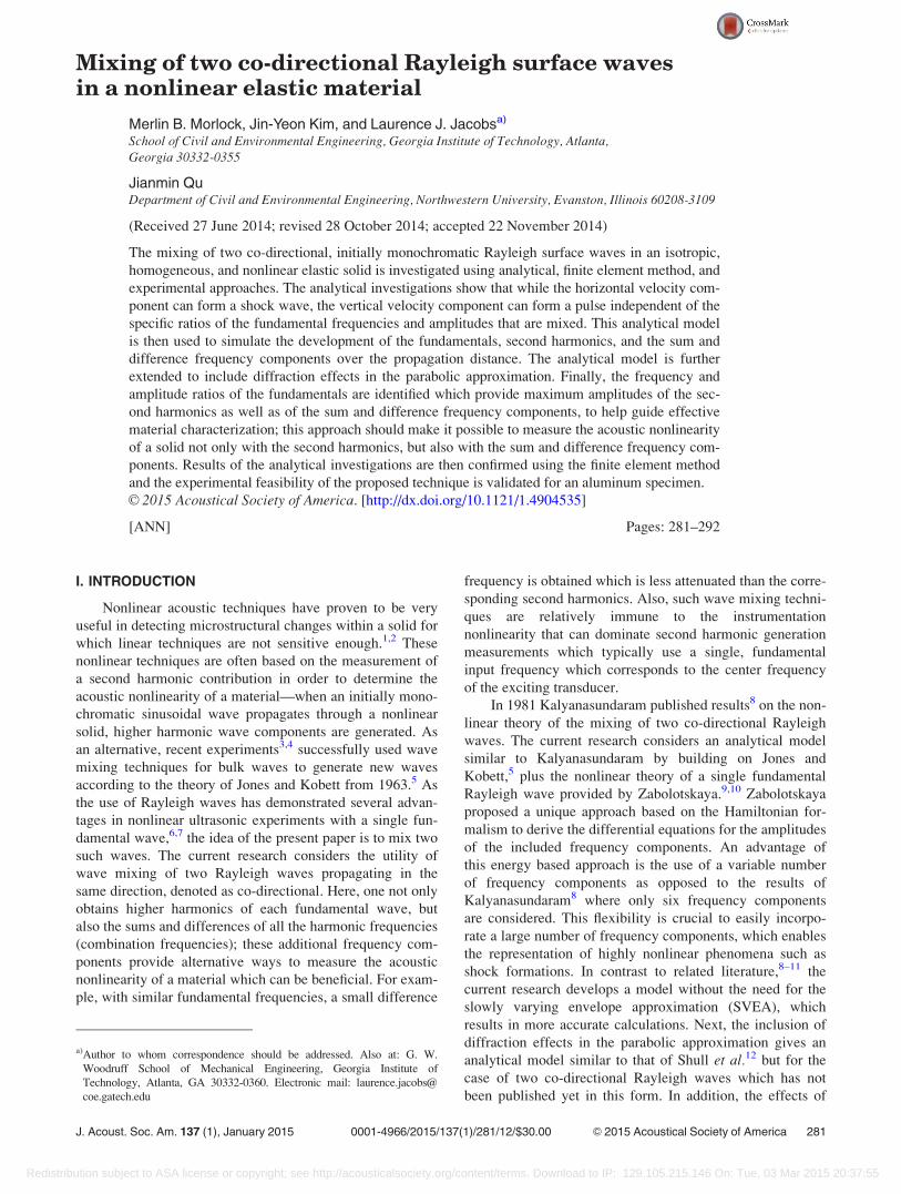
Mixing of two co-directional Rayleigh surface waves in a nonlinear elastic material Merlin B. Morlock, Jin-Yeon Kim, and Laurence J. Jacobs a) School of Civil and Environmental Engineering, Georgia Institute of Technology, Atlanta, Georgia 30332-0355 Jianmin Qu Department of Civil and Environmental Engineering, Northwestern University, Evanston, Illinois 60208-3109 (Received 27 June 2014; revised 28 October 2014; accepted 22 November 2014) The mixing of two co-directional, initially monochromatic Rayleigh surface waves in an isotropic, homogeneous, and nonlinear elastic solid is investigated using analytical, finite element method, and experimental approaches. The analytical investigations show that while the horizontal velocity com- ponent can form a shock wave, the vertical velocity component can form a pulse independent of the specific ratios of the fundamental frequencies and amplitudes that are mixed. This analytical model is then used to simulate the development of the fundamentals, second harmonics, and the sum and difference frequency components over the propagation distance. The analytical model is further extended to include diffraction effects in the parabolic approximation. Finally, the frequency and amplitude ratios of the fundamentals are identified which provide maximum amplitudes of the sec- ond harmonics as well as of the sum and difference frequency components, to help guide effective material characterization; this approach should make it possible to measure the acoustic nonlinearity of a solid not only with the second harmonics, but also with the sum and difference frequency com- ponents. Results of the analytical investigations are then confirmed using the finite element method and the experimental feasibility of the proposed technique is validated for an aluminum specimen. V C 2015 Acoustical Society of America.[http://dx.doi.org/10.1121/1.4904535] [ANN] Pages: 281–292 I. INTRODUCTION Nonlinear acoustic techniques have proven to be very useful in detecting microstructural changes within a solid for which linear techniques are not sensitive enough. 1,2 These nonlinear techniques are often based on the measurement of a second harmonic contribution in order to determine the acoustic nonlinearity of a material—when an initially mono- chromatic sinusoidal wave propagates through a nonlinear solid, higher harmonic wave components are generated. As an alternative, recent experiments 3,4 successfully used wave mixing techniques for bulk waves to generate new waves according to the theory of Jones and Kobett from 1963. 5 As the use of Rayleigh waves has demonstrated several advan- tages in nonlinear ultrasonic experiments with a single fun- damental wave, 6,7 the idea of the present paper is to mix two such waves. The current research considers the utility of wave mixing of two Rayleigh waves propagating in the same direction, denoted as co-directional. Here, one not only obtains higher harmonics of each fundamental wave, but also the sums and differences of all the harmonic frequencies (combination frequencies); these additional frequency com- ponents provide alternative ways to measure the acoustic nonlinearity of a material which can be beneficial. For exam- ple, with similar fundamental frequencies, a small difference frequency is obtained which is less attenuated than the corre- sponding second harmonics. Also, such wave mixing techni- ques are relatively immune to the instrumentation nonlinearity that can dominate second harmonic generation measurements which typically use a single, fundamental input frequency which corresponds to the center frequency of the exciting transducer. In 1981 Kalyanasundaram published results 8 on the non- linear theory of the mixing of two co-directional Rayleigh waves. The current research considers an analytical model similar to Kalyanasundaram by building on Jones and Kobett, 5 plus the nonlinear theory of a single fundamental Rayleigh wave provided by Zabolotskaya. 9,10 Zabolotskaya proposed a unique approach based on the Hamiltonian for- malism to derive the differential equations for the amplitudes of the included frequency components. An advantage of this energy based approach is the use of a variable number of frequency components as opposed to the results of Kalyanasundaram 8 where only six frequency components are considered. This flexibility is crucial to easily incorpo- rate a large number of frequency components, which enables the representation of highly nonlinear phenomena such as shock formations. In contrast to related literature, 8–11 the current research develops a model without the need for the slowly varying envelope approximation (SVEA), which results in more accurate calculations. Next, the inclusion of diffraction effects in the parabolic approximation gives an analytical model similar to that of Shull et al. 12 but for the case of two co-directional Rayleigh waves which has not been published yet in this form. In addition, the effects of a) Author to whom correspondence should be addressed. Also at: G. W. Woodruff School of Mechanical Engineering, Georgia Institute of Technology, Atlanta, GA 30332-0360. Electronic mail: laurence.jacobs@ coe.gatech.edu J. Acoust. Soc. Am. 137 (1), January 2015 V C 2015 Acoustical Society of America 281 0001-4966/2015/137(1)/281/12/$30.00 Redistribution subject to ASA license or copyright; see http://acousticalsociety.org/content/terms. Download to IP: 129.105.215.146 On: Tue, 03 Mar 2015 20:37:55
-
Upload
duongnguyet -
Category
Documents
-
view
216 -
download
0
Transcript of Mixing of two co-directional Rayleigh surface waves in a … Papers/Qu - JASA... · 2015-03-03 ·...
Mixing of two co-directional Rayleigh surface wavesin a nonlinear elastic material
Merlin B. Morlock, Jin-Yeon Kim, and Laurence J. Jacobsa)
School of Civil and Environmental Engineering, Georgia Institute of Technology, Atlanta,Georgia 30332-0355
Jianmin QuDepartment of Civil and Environmental Engineering, Northwestern University, Evanston, Illinois 60208-3109
(Received 27 June 2014; revised 28 October 2014; accepted 22 November 2014)
The mixing of two co-directional, initially monochromatic Rayleigh surface waves in an isotropic,
homogeneous, and nonlinear elastic solid is investigated using analytical, finite element method, and
experimental approaches. The analytical investigations show that while the horizontal velocity com-
ponent can form a shock wave, the vertical velocity component can form a pulse independent of the
specific ratios of the fundamental frequencies and amplitudes that are mixed. This analytical model
is then used to simulate the development of the fundamentals, second harmonics, and the sum and
difference frequency components over the propagation distance. The analytical model is further
extended to include diffraction effects in the parabolic approximation. Finally, the frequency and
amplitude ratios of the fundamentals are identified which provide maximum amplitudes of the sec-
ond harmonics as well as of the sum and difference frequency components, to help guide effective
material characterization; this approach should make it possible to measure the acoustic nonlinearity
of a solid not only with the second harmonics, but also with the sum and difference frequency com-
ponents. Results of the analytical investigations are then confirmed using the finite element method
and the experimental feasibility of the proposed technique is validated for an aluminum specimen.VC 2015 Acoustical Society of America. [http://dx.doi.org/10.1121/1.4904535]
[ANN] Pages: 281–292
I. INTRODUCTION
Nonlinear acoustic techniques have proven to be very
useful in detecting microstructural changes within a solid for
which linear techniques are not sensitive enough.1,2 These
nonlinear techniques are often based on the measurement of
a second harmonic contribution in order to determine the
acoustic nonlinearity of a material—when an initially mono-
chromatic sinusoidal wave propagates through a nonlinear
solid, higher harmonic wave components are generated. As
an alternative, recent experiments3,4 successfully used wave
mixing techniques for bulk waves to generate new waves
according to the theory of Jones and Kobett from 1963.5 As
the use of Rayleigh waves has demonstrated several advan-
tages in nonlinear ultrasonic experiments with a single fun-
damental wave,6,7 the idea of the present paper is to mix two
such waves. The current research considers the utility of
wave mixing of two Rayleigh waves propagating in the
same direction, denoted as co-directional. Here, one not only
obtains higher harmonics of each fundamental wave, but
also the sums and differences of all the harmonic frequencies
(combination frequencies); these additional frequency com-
ponents provide alternative ways to measure the acoustic
nonlinearity of a material which can be beneficial. For exam-
ple, with similar fundamental frequencies, a small difference
frequency is obtained which is less attenuated than the corre-
sponding second harmonics. Also, such wave mixing techni-
ques are relatively immune to the instrumentation
nonlinearity that can dominate second harmonic generation
measurements which typically use a single, fundamental
input frequency which corresponds to the center frequency
of the exciting transducer.
In 1981 Kalyanasundaram published results8 on the non-
linear theory of the mixing of two co-directional Rayleigh
waves. The current research considers an analytical model
similar to Kalyanasundaram by building on Jones and
Kobett,5 plus the nonlinear theory of a single fundamental
Rayleigh wave provided by Zabolotskaya.9,10 Zabolotskaya
proposed a unique approach based on the Hamiltonian for-
malism to derive the differential equations for the amplitudes
of the included frequency components. An advantage of
this energy based approach is the use of a variable number
of frequency components as opposed to the results of
Kalyanasundaram8 where only six frequency components
are considered. This flexibility is crucial to easily incorpo-
rate a large number of frequency components, which enables
the representation of highly nonlinear phenomena such as
shock formations. In contrast to related literature,8–11 the
current research develops a model without the need for the
slowly varying envelope approximation (SVEA), which
results in more accurate calculations. Next, the inclusion of
diffraction effects in the parabolic approximation gives an
analytical model similar to that of Shull et al.12 but for the
case of two co-directional Rayleigh waves which has not
been published yet in this form. In addition, the effects of
a)Author to whom correspondence should be addressed. Also at: G. W.
Woodruff School of Mechanical Engineering, Georgia Institute of
Technology, Atlanta, GA 30332-0360. Electronic mail: laurence.jacobs@
coe.gatech.edu
J. Acoust. Soc. Am. 137 (1), January 2015 VC 2015 Acoustical Society of America 2810001-4966/2015/137(1)/281/12/$30.00
Redistribution subject to ASA license or copyright; see http://acousticalsociety.org/content/terms. Download to IP: 129.105.215.146 On: Tue, 03 Mar 2015 20:37:55

different amplitudes and frequencies of the fundamental
waves and of the corresponding ratios are discussed.
Formulas are derived to calculate the acoustic nonlinearity
of a material similar to the case of a single fundamental
Rayleigh wave investigated by Herrmann et al.,6 but not
only based on the second harmonics but also on the sum and
difference frequency components. Finally, results from the
analytical model are compared to results from a finite ele-
ment model for validation purposes.
The overall objective of this research is to provide mod-
els that support experiments and enable the interpretation of
the measured data and the selection of the amplitudes and
frequencies of the two fundamental waves, in order to maxi-
mize the amplitudes of the second harmonics, as well as
those of the sum and difference frequency components. This
can help to enhance measurements by providing an
improved signal-to-noise ratio (SNR), which enables a more
accurate determination of the acoustic nonlinearity of a ma-
terial; this research demonstrates the feasibility and potential
of co-directional Rayleigh wave mixing in order to experi-
mentally quantify the acoustic nonlinearity of a solid, analo-
gously to longitudinal waves, in multiple ways within a
single measurement.
II. ANALYTICAL MODEL
A. Modeling
Consider an isotropic, homogeneous, elastic and weakly
nonlinear material. In order to determine significant solu-
tions to the nonlinear Rayleigh wave equation, it is a good
approximation to only take frequency components into
account for which resonance is fulfilled. It is assumed in the
following that the resonance condition of Jones and Kobett5
holds similarly for Rayleigh waves which can be written as
xa6xbð Þpc
¼ ka6kb !jpj¼1 jxa6xbj
c¼ jka6kbj: (1)
Here, c is the wave speed, p the propagation direction,
jxa6xbj the angular frequency, and jka6kbj the wavenum-
ber of the generated and significant wave. Moreover, ka and
kb as well as xa and xb are the wave vectors and angular fre-
quencies of the two fundamental waves that are mixed. The
absolute values jkaj ¼ ka and jkbj ¼ kb are the correspond-
ing wavenumbers. As we are interested in nonlinear ultra-
sonic measurements where fundamental Rayleigh waves are
compared to nonlinearly generated Rayleigh waves, we want
this generation to be directly out of the interaction of the fun-
damentals to obtain larger amplitudes and a better SNR.
Consequently, the wave speed c of the generated wave
within Eq. (1) is set to the Rayleigh wave speed cr which
results in
ðxa6xbÞ2 ¼ x2a þ x2
b 6 2xaxb cosðHÞ; (2)
where H is the angle between the fundamental wave vectors.
This leads to cosðHÞ ¼ 1 and confirms that the resonance
condition is only fulfilled for co-directional mixing.
As the individual fundamentals also fulfill the resonance
condition which leads to second harmonics, it can be con-
cluded that both of the second harmonics as well as the sum
and difference frequency components are directly generated
from the fundamentals, and are therefore of critical interest
for experiments. By generalizing the co-directional mixing
of the two fundamentals, it follows that the generated waves
interact again with all other waves leading to the formation
of all kinds of higher harmonics and combination frequen-
cies. They can be written as nxa, mxb, and jnxa6mxbj for
n¼ 1, 2, 3, and m¼ 1, 2, 3. Moreover, it is assumed that the
solution of the nonlinear problem is close to the solution of
the corresponding linear problem.9 Consequently, the solu-
tion form for the displacements in the x- and z-directions for
co-directional Rayleigh wave mixing in a semi-infinite solid
in the z< 0 half-space with the surface at z¼ 0 can be writ-
ten as
ux ¼X
n
bne�inxat|fflfflfflfflffl{zfflfflfflfflffl}an
in
jnj n1ejnjkan1z þ gejnjkan2z� �
|fflfflfflfflfflfflfflfflfflfflfflfflfflfflfflfflfflfflfflfflfflffl{zfflfflfflfflfflfflfflfflfflfflfflfflfflfflfflfflfflfflfflfflfflffl}uxn
einkax;
(3a)
uz ¼X
n
bne�inxat|fflfflfflfflffl{zfflfflfflfflffl}an
ðejnjkan1z þ gn2ejnjkan2zÞ|fflfflfflfflfflfflfflfflfflfflfflfflfflfflfflfflfflffl{zfflfflfflfflfflfflfflfflfflfflfflfflfflfflfflfflfflffl}uzn
einkax: (3b)
The material dependent constants g, n1, and n2 are defined
elsewhere.9 The imaginary unit is denoted by i and all waves
propagate in the positive x-direction. The variable bn repre-
sents the displacement amplitudes of the different frequency
components that are in demand. Moreover, each n describes
a distinct frequency component, and negative n are the corre-
sponding complex conjugates resulting in a�n ¼ a�n and
b�n ¼ b�n.
One thing that distinguishes Eqs. (3a) and (3b) from the
work of Kalyanasundaram8 is that all frequency components
are pulled into only one summation for each displacement
direction. This leads to a special definition of the control
variable n. With the frequency mixing ratio (FMR) /¼ xb=xa and 0 < / < 1 without loss of generality, n takes
the values
61;62;…;6/;62/;…;616/;626/;6162/;
6262/;…;617/;627/;6172/;6272/; ::: :
(4)
Integers and multiples of / represent harmonics, whereas
the other terms denote combination frequency components.
The zero frequency is not considered.
As Eqs. (3a) and (3b) are analogous to the solution form
Zabolotskaya postulated,9 we can take advantage of the cor-
responding derivation to solve for the unknown and varying
bn. To follow the approach of Zabolotskaya in obtaining the
kinetic and elastic energy, one needs to integrate over a dis-
tance in the x-direction that contains full periods of all fre-
quencies involved. If xa and xb are decimals with a finite
number of decimal places, fractions of such decimals or if
numbers with infinite decimal places cancel out in the FMR,
282 J. Acoust. Soc. Am., Vol. 137, No. 1, January 2015 Morlock et al.: Mixing of Rayleigh surface waves
Redistribution subject to ASA license or copyright; see http://acousticalsociety.org/content/terms. Download to IP: 129.105.215.146 On: Tue, 03 Mar 2015 20:37:55

then one can always find such a distance. When such a gen-
eral case is considered, the kinetic energy T as well as the
elastic energies V and W can be written analogously to
Zabolotskaya9 but with n given in Eq. (4). The energies are
then used for the Lagrange equations of the second kind for
the so far conservative system. The Lagrangian follows as
L ¼ T � V �W and the different a�n are chosen as gener-
alized coordinates. Based on the expressions used by
Zabolotskaya,9 the generalized momenta @L=@ _a�n are equal
to @T =@ _a�n ¼ M _an=ð2jnjÞ. The other necessary term for the
equations of motion is given by @L=@a�n ¼ �@V=@a�n
�@W=@a�n. Here, @V=@a�n ¼ Mx2ajnjan=2 holds, where M
depends on material properties and contains the wavenumber
ka. In order to calculate the partial derivative of W with
respect to a�n,
W ¼ lk2a
Xn¼mþl
wnlma�namal (5)
is utilized, where n has been replaced by �n within the
summation when compared to Zabolotskaya.9 Note that
wnlm stays unchanged as it only contains absolute values of
n and the condition n¼mþ l needs to be fulfilled. This
yields
@W@a�n
¼ �jnjlk2a
Xn¼mþl
mlSmlbmble�i mþlð Þxat: (6)
The variables wnlm as well as Sml, given by Zabolotskaya,9
solely depend on material properties and l denotes the
shear modulus of the solid. Also, m and l are control varia-
bles like n. This leads to the Lagrange equations of the sec-
ond kind of
M
2jnj€bn � 2inxa
_bn � n2x2abn
� �e�inxat
¼ �Mx2a
2jnjbne�inxat þ jnjlk2
a
�X
n¼mþl
mlSmlbmble�i mþlð Þxat: (7)
Making the assumption of periodic steady-state waves,9
i.e., @bn=@t ¼ @2bn=@t2 ¼ 0, one can evaluate the total
derivative _bn ¼ @bn=@tþ cr@bn=@x ¼ cr@bn=@x. Similarly, €bn
¼ c2r@
2bn=@x2. Based on these expressions, a multiplication of
Eq. (7) with einxat gives
� 1
2inka
@2bn
@x2þ @bn
@x¼ inlxa
Mc3r
Xn¼mþl
mlSmlbmbl � an2bn:
(8)
Here, an attenuation term has been implemented analogously
to the literature9,13 with the attenuation coefficient a. The
first term on the right-hand side describes wave interactions
caused by both geometric and material nonlinearities that
lead to the generation of higher harmonics and combination
frequency components. Equation (8) represents a system of
coupled second order ordinary differential equations with
quadratic terms, since the incorporated elastic energy is of
cubic order.
As a next step, the time derivatives of the displacements
need to be established to investigate particle velocities later
on. They are similar to Zabolotskaya9 given by
_ux ¼ vx ¼X
n
vne�inxatuxneinkax; (9a)
_uz ¼ vz ¼X
n
vne�inxatuzneinkax; (9b)
with the particle velocity amplitude of the different fre-
quency components vn ¼ cr@bn=@x� inxabn.
In a case where the amplitudes of the frequency
components under consideration change slowly, it is com-
mon to use the SVEA.8–11 This means that if j@2bn=@x2j� j2nka@bn=@xj holds the highest order derivative @2bn=@x2
can be neglected14 within Eq. (8). The result is equivalent to
Zabolotskaya’s formula for a single fundamental wave,9 but
with a different definition of n and the equation is formulated
with bn instead of vn. With the SVEA these amplitudes are
related by9
vn ¼ �inxabn: (10)
B. Simulation
A characteristic quantity in wave propagation is the dis-
continuity distance which will be used for numerical analy-
ses. At this distance, the slope of the waveform of the
particle velocity becomes infinitely large for a hypothetical
lossless nonlinear material.15 Based on the discontinuity dis-
tances for a single fundamental bulk wave13 and a single
fundamental Rayleigh wave,16 the empirical formula for the
discontinuity distance of two co-directionally mixed
Rayleigh waves can be written as
xd ¼Mc3
r
8ljS11jxa jbICaj þ /jbICbjð Þ ; (11)
where S11 denotes Sml for m¼ l¼ 1. This equation is related
to the expression for a single fundamental bulk wave by
Eq. (21) and to the expression for a single fundamental
Rayleigh wave by Eq. (10). The quantities bICa and bICb
denote the initial values of b1 and b/ and the ratio bICb /bICa
is called the amplitude mixing ratio (AMR).
To reduce the computational complexity at highly non-
linear effects such as shocks, the SVEA will be utilized for
the simulation of Eq. (8) in the following. Here, the behavior
of the waveforms and the development of the displacement
amplitudes in the case of low attenuation will be simulated
numerically with MATHEMATICA 9.0.
1. Waveforms
For an easier comparison to the behavior of a single fun-
damental Rayleigh wave, assume the same steel material
properties as in the literature9 which are given in Table I. The
amplitudes bICa and bICb are chosen of the same dimension as
the fundamentals of longitudinal waves.17 The initial ampli-
tudes of all other frequency components are set to zero.
Moreover, it is crucial to select low values for the attenuation
J. Acoust. Soc. Am., Vol. 137, No. 1, January 2015 Morlock et al.: Mixing of Rayleigh surface waves 283
Redistribution subject to ASA license or copyright; see http://acousticalsociety.org/content/terms. Download to IP: 129.105.215.146 On: Tue, 03 Mar 2015 20:37:55

coefficient to be able to observe effects such as shock forma-
tions before the waves decay. However, a simulation with a
very small attenuation coefficient can be numerically difficult
to handle and consequently a balance should be found.
The waveforms of the particle velocities are illustrated
in Fig. 1 for two different FMRs. Here, all plots are normal-
ized to vx0 which denotes the initial amplitude of vx. The hor-
izontal axis represents the dimensionless variable
s ¼ xaðt� x=crÞ=2p. In plots (a1) and (b1) the horizontal
velocity component forms a shock while in plots (a2) and
(b2) a pulse arises in the vertical velocity component with an
increasing propagation distance x. This behavior has been
similarly shown by Zabolotskaya9 but not for the case of co-
directional Rayleigh wave mixing as presented here.
Moreover, these effects occur independently of the FMR.
The increased peaks indicate that the energy is shifted to the
surface when higher frequencies are generated since they
have lower penetration depths.9,10 Additionally, the largest
peaks get larger for a higher FMR. In contrast, very different
fundamental frequencies lead to less sharp peaks as they
have different energy transfer characteristics and do not
form a shock and pulse at similar propagation distances in
the case of comparable initial fundamental displacement
amplitudes. Therefore, the amplitudes in plots (b1) and (b2)
will decline until the smaller fundamental frequency gener-
ates a second shock and pulse, at propagation distances that
are larger than the illustrated ones.
In addition, a shock and pulse can be formed independ-
ently of the AMR and for large FMRs as in (a1) and (a2) a
beat can occur.
2. Displacement amplitudes
In the following, the development over the propagation
distance of the displacement amplitudes bn of the fundamen-
tals, second harmonics as well as of the sum and difference
frequency components is discussed. They are typically the
largest, and therefore the most attractive components in
TABLE I. Material properties.
Material Young’s modulus E Poisson’s ratio r Mass density q Third order elastic constants A, B, C
Steel 2� 1011 N/m2 0.27 7850 kg/m3 �7.6� 1011 N/m2 �2.5� 1011 N/m2 �9� 1010 N/m2
Fused quartz 7.17� 1010 N/m2 0.17 2203 kg/m3 �5.28� 1010 N/m2 5.4� 1010 N/m2 2.15� 1011 N/m2
Aluminum 7.09� 1010 N/m2 0.34 2700 kg/m3 �3.5� 1011 N/m2 �1.5� 1011 N/m2 �1.03� 1011N/m2
FIG. 1. (Color online) Normalized waveforms of the horizontal (a1), (b1) and the vertical (a2), (b2) particle velocity component at z¼ 0. The attenuation coef-
ficient is set to a¼ 6� 10�4 Np/m and the fundamental frequency xa¼ 5p� 106 rad/s is fixed while xb¼ 4p� 106 rad/s (a1), (a2) as well as xb¼p� 106 rad/s
(b1), (b2). The initial conditions are chosen as bICa¼ bICb¼ i7.5� 10�10 m. All frequencies up to the 120th harmonic of each fundamental wave and all com-
bination frequencies up to 60xa 6 60xb are included.
284 J. Acoust. Soc. Am., Vol. 137, No. 1, January 2015 Morlock et al.: Mixing of Rayleigh surface waves
Redistribution subject to ASA license or copyright; see http://acousticalsociety.org/content/terms. Download to IP: 129.105.215.146 On: Tue, 03 Mar 2015 20:37:55

nonlinear ultrasonic measurements. Simulations are per-
formed for fused quartz given in Table I to facilitate compar-
isons to Kalyanasundaram.8 The results for two different
FMRs are illustrated in Fig. 2. As purely imaginary values
for bICa and bICb are utilized, the different bn also remain as
imaginary—this is analogous to the findings of
Kalyanasundaram.8 The reason for this behavior is that the
change of the displacement amplitudes @bn/@x within the
simulated equations equals an imaginary quantity.
The plots show that the energy transfer is larger for
higher frequencies. On the one hand this means that the
attenuation is obviously larger for higher frequencies, which
can be observed, among others, for the difference frequency
component at large propagation distances. On the other
hand, the absolute value of the slope for small propagation
distances tends to be larger if the frequency under considera-
tion is higher (and the corresponding fundamental frequen-
cies in the case that a non-fundamental component is
investigated). Thus, the initial slopes of the 2xb and the sum
frequency components are larger in plot (a), since these and
the corresponding fundamental xb component have higher
frequencies.
A more complicated behavior is present within the ini-
tial development of the difference frequency component—as
a high FMR results in a small difference frequency, and vice
versa, the development of the difference frequency compo-
nent depends on a balance of its own frequency and the fun-
damental frequencies. Therefore, the negative rise within
plots (a) and (b) appears to be pretty much the same for
small propagation distances.
These results are partially in line with the work of
Kalyanasundaram.8 The xb component changes more slowly
for small FMRs in both models. For the sum and difference
frequency components, the signs and the dependence of the
initial slope on the FMR match relatively well. However,
Kalyanasundaram states that for larger FMRs, the fundamen-
tals as well as the sum and difference frequency components
reach their first minima or maxima faster. This is not the
case for the xa and the difference frequency components in
the plots presented here. Also note that the overall behavior
of the xa component is quite different. These discrepancies
could be due to differing simulation parameters and model-
ing approaches. Especially, the number of included fre-
quency components can be important if the propagation
distances are large enough. Investigations have shown that
for the utilized setups and considered propagation distance,
more frequency components than only the fundamentals,
second harmonics as well as the sum and difference frequen-
cies as included by Kalyanasundaram are necessary to obtain
an accurate development of these six components.
C. Implementation of diffraction effects
In addition to the nonlinear interaction and attenuation,
diffraction effects can also be important to account for in
nonlinear Rayleigh wave experiments, since they are often
conducted in the far field where these effects might have a
significant influence. Consequently, the model derived is
extended to include these diffraction effects. Additionally,
the SVEA is applied again to simplify the modeling and the
computations as a system of coupled partial differential
equations will be obtained and numerically solved.
The starting point of the derivation is the assumption of
narrow angle diffraction which can be described using a para-
bolic approximation.12,18 Suppose that the wave vector of dif-
fracted Rayleigh waves can be written as nka ¼ nðkx; ky; 0ÞT .
Then the introduction of the small angle d between the wave
propagation direction and the x axis yields nkx ¼ nka cosðdÞand nky ¼ nka sinðdÞ. These wavenumbers can be approxi-
mated with a Taylor series around d¼ 0 as nkx � nkað1�d2=2Þ and nky � nkad. The solution form of Eqs. (3a) and
(3b) follows now as
ux ¼X
n
bneinkað�d2x=2þdyÞ|fflfflfflfflfflfflfflfflfflfflfflffl{zfflfflfflfflfflfflfflfflfflfflfflffl}bdn
uxneinðkax�xatÞ; (12a)
uz ¼X
n
bneinkað�d2x=2þdyÞ|fflfflfflfflfflfflfflfflfflfflfflffl{zfflfflfflfflfflfflfflfflfflfflfflffl}bdn
uzneinðkax�xatÞ; (12b)
FIG. 2. (Color online) Normalized displacement amplitudes of selected frequency components over the propagation distance. The attenuation coefficient is set
to a¼ 6� 10�4 Np/m and the fundamental frequency xa¼ 5p� 106 rad/s is fixed while xb¼ 4p� 106 rad/s (a) as well as xb¼p� 106 rad/s (b). The initial
conditions are chosen as bICa¼ bICb¼ i7.5� 10�10m. All frequencies up to the 120th harmonic of each fundamental wave and all combination frequencies up
to 60xa 6 60xb are included.
J. Acoust. Soc. Am., Vol. 137, No. 1, January 2015 Morlock et al.: Mixing of Rayleigh surface waves 285
Redistribution subject to ASA license or copyright; see http://acousticalsociety.org/content/terms. Download to IP: 129.105.215.146 On: Tue, 03 Mar 2015 20:37:55
where bdn denotes the diffracted displacement amplitudes
and is a function of x and y. Eventually, one can calculate
the partial derivatives
@bdn
@x¼ � inka
2d2bneinka �d2x=2þdyð Þ þ @bn
@xeinka �d2x=2þdyð Þ
(13)
and
i
2nka
@2bdn
@y2¼ � inka
2d2bneinka �d2x=2þdyð Þ: (14)
Now, Eqs. (13) and (14) are combined and @bn/@x is substi-
tuted by the expression of Eq. (8) after applying the SVEA.
This leads to
1
2inka
@2bdn
@y2þ @bdn
@x
¼ inlxa
Mc3r
Xn¼mþl
mlSmlbdmbdl � an2bdn: (15)
The model obtained is very similar to the case of a single
fundamental wave.12 The main differences are again that ntakes different values, and the formulation presented is writ-
ten for the displacement amplitudes instead of the particle
velocity amplitudes.
D. Simplified analytical model
1. General approach
In nonlinear ultrasonic experiments, having sufficiently
large amplitudes of the frequency components under consid-
eration is crucial to facilitate measurements with an
improved SNR. In order to find combinations of initial fun-
damental amplitudes and frequencies that maximize the
amplitudes of the second harmonics, and the sum and the
difference frequency components, a general approach with a
simplified model will be discussed as an alternative to a
case-by-case investigation. The SVEA is applied and attenu-
ation as well as diffraction effects are assumed to be negligi-
ble which is often a good approximation for small
propagation distances. Additionally, for such distances the
fundamentals are almost unaffected by other frequency com-
ponents and they represent the only significant impact on the
second harmonics, as well as on the sum and difference fre-
quency components.
Based on these assumptions as well as based on Eqs. (8)
and (15), the displacement amplitudes of the fundamentals
become
@b1
@x¼ 0! b1 ¼ bICa ¼ constant; (16a)
@b/
@x¼ 0! b/ ¼ bICb ¼ constant: (16b)
The displacement amplitudes of the second harmonics as
well as of the sum and difference frequency components are
given by
bn ¼inlxax
Mc3r
Xn¼mþl
mlSmlbmbl; (17)
where bm and bl solely represent fundamental displacement
amplitudes. Thus, the second harmonics depend on the
square of the corresponding fundamental displacement am-
plitude, whereas the sum and difference frequency compo-
nents depend on the product of both fundamental
displacement amplitudes. Consequently, the choice of the
initial fundamental displacement amplitudes is evident—the
product jbmblj should be maximized for the component of in-
terest within the given experimental constraints, for exam-
ple, by choosing an appropriate AMR.
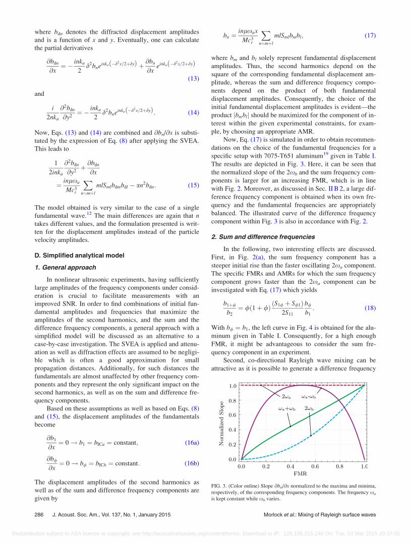
Now, Eq. (17) is simulated in order to obtain recommen-
dations on the choice of the fundamental frequencies for a
specific setup with 7075-T651 aluminum19 given in Table I.
The results are depicted in Fig. 3. Here, it can be seen that
the normalized slope of the 2xb and the sum frequency com-
ponents is larger for an increasing FMR, which is in line
with Fig. 2. Moreover, as discussed in Sec. II B 2, a large dif-
ference frequency component is obtained when its own fre-
quency and the fundamental frequencies are appropriately
balanced. The illustrated curve of the difference frequency
component within Fig. 3 is also in accordance with Fig. 2.
2. Sum and difference frequencies
In the following, two interesting effects are discussed.
First, in Fig. 2(a), the sum frequency component has a
steeper initial rise than the faster oscillating 2xa component.
The specific FMRs and AMRs for which the sum frequency
component grows faster than the 2xa component can be
investigated with Eq. (17) which yields
b1þ/
b2
¼ / 1þ /ð Þ S1/ þ S/1ð Þ2S11
b/
b1
: (18)
With b/ ¼ b1, the left curve in Fig. 4 is obtained for the alu-
minum given in Table I. Consequently, for a high enough
FMR, it might be advantageous to consider the sum fre-
quency component in an experiment.
Second, co-directional Rayleigh wave mixing can be
attractive as it is possible to generate a difference frequency
FIG. 3. (Color online) Slope @bn/@x normalized to the maxima and minima,
respectively, of the corresponding frequency components. The frequency xa
is kept constant while xb varies.
286 J. Acoust. Soc. Am., Vol. 137, No. 1, January 2015 Morlock et al.: Mixing of Rayleigh surface waves
Redistribution subject to ASA license or copyright; see http://acousticalsociety.org/content/terms. Download to IP: 129.105.215.146 On: Tue, 03 Mar 2015 20:37:55

component b1�/ which grows much faster than a second har-
monic ~b2 of a single fundamental wave at the same fre-
quency. By making use of Eq. (17) and by selecting the
initial fundamental displacement amplitudes b1 and b�/ of
the mixing case as half the initial fundamental displacement
amplitude of the single wave case, the ratio
b1�/
~b2
¼ �/1� /ð Þ
S1;�/ þ S�/1ð Þ2S11
(19)
can be found. Note that a comma is introduced in S1;�/ to
clearly show that two different indices are involved. A simu-
lation result is given in Fig. 4 for aluminum of Table I. It can
be seen that for high FMRs the mixing method is clearly
beneficial. The reason is that a high FMR in the mixing case
implies much larger fundamental frequencies when com-
pared to the case of a single fundamental wave. As a conse-
quence, the energy transfer from the fundamentals is much
higher in the former case, which finally leads to a larger ratio
b1�/=~b2.
E. Acoustic nonlinearity parameter
1. Modeling
One of the major objectives in nonlinear ultrasonic
experiments is the measurement of the acoustic nonlinearity
parameter (ANP) of a material. Therefore, the existing defi-
nition of the ANP within the literature6,12 is extended to the
case of co-directional Rayleigh wave mixing. By using the
expression of the ANP for longitudinal waves analogously
for Rayleigh waves, the definition
b ¼ 8b2
k2ab2
1x(20)
in terms of the higher fundamental frequency is obtained
which is based on and proportional to the definition by
Herrmann et al.6 As the ANP is a material property, a formu-
lation can be specified which only depends on the solid
under consideration. This is realized by inserting the dis-
placement amplitudes b1 and b2 of a Rayleigh wave model
into Eq. (20), at which the model is based on the same
assumptions that led to this equation. These assumptions
neglect both attenuation and diffraction effects, as well as
assume a constant fundamental and a linearly changing sec-
ond harmonic amplitude over the propagation distance.13,20
Since all these points are incorporated within the simplified
analytical model of Sec. II D, the corresponding displace-
ment amplitudes are used to express the ANP only with ma-
terial constants as
bmat ¼16ilS11
Mc2r ka
; (21)
which is given in a similar way by Shull et al.12 Note that
the wavenumber cancels out.
Now, for co-directional Rayleigh wave mixing, it might
be desirable to calculate a similar ANP with both second har-
monics as well as with the sum and difference frequency
components. This results in a high flexibility in choosing the
most attractive frequency component for a specific problem
and the possibility to compare the results. In a fashion analo-
gous to Eq. (20), the general expression for the four different
ANPs is defined as
bml ¼16sgn mlð Þbmþl
mþ lð Þkjmjkjljbmblx: (22)
Here, m and l are either 1 or 6/ and mþ l is 2; 2/; 1þ /;or 1� /. Moreover, k1¼ ka as well as k/ ¼ kb and sgn
denotes the sign function. Thus, b11 equals b of Eq. (20).
Subsequently, bml is related to b. With Eq. (17), the general
relationship between the different ANPs can be stated as
b ¼ bml
S11Xmþl¼iþj
Sij
: (23)
The variable Sij corresponds to Sml with new control varia-
bles at which i and j are either 1 or 6/.
2. Simulation
Next, the variation of the ANP b calculated in four dif-
ferent ways according to Eq. (23) is investigated when
including the interaction, attenuation and diffraction effects.
Therefore, Eq. (15) is simulated and Gaussian sources16 of
saðyÞ ¼ bICae�ðy=rÞ2 and sbðyÞ ¼ bICbe�ðy=rÞ2 are used for the
corresponding fundamental waves. Here, a value of
r¼ 6.35 mm is chosen which represents the radius of the
wedge transducer utilized in Sec. IV for the experiments. At
the limits in the y-direction, all the bn’s are set to zero.
The results of a simulation with the aluminum of
Table I are presented in Fig. 5. Here, all curves are normal-
ized to bmat. Consequently, the four formulations of the ANP
b yield indeed approximately the same absolute value of
jbmatj at small propagation distances and deviate for larger
propagation distances because of the interaction, attenuation,
and diffraction effects. This confirms, on the one hand, the
assumptions made in the simplified analytical model and, on
the other hand, Eqs. (21) and (23) for small propagation dis-
tances which have been derived based on these assumptions.
Thus, for such distances and measurements of absolute dis-
placements, it might be possible to approximately obtain
bmat in four ways within an experiment.
FIG. 4. (Color online) Amplitude ratios over the FMR.
J. Acoust. Soc. Am., Vol. 137, No. 1, January 2015 Morlock et al.: Mixing of Rayleigh surface waves 287
Redistribution subject to ASA license or copyright; see http://acousticalsociety.org/content/terms. Download to IP: 129.105.215.146 On: Tue, 03 Mar 2015 20:37:55

In addition, in Fig. 5, the ANP formulations related to
the second harmonics and the sum frequency component rise
in the beginning as the diffraction effects are higher for
lower frequencies. Consequently, the fundamentals are more
reduced than the second harmonics and the sum frequency
component. In contrast, as the difference frequency is much
smaller than both of the fundamental frequencies, the corre-
sponding ANP formulation initially drops. At larger distan-
ces attenuation becomes the dominant effect on the different
curves.
III. FINITE ELEMENT MODEL
A. Modeling
As a next step, a simplified model using the finite ele-
ment method (FEM) is set up with COMSOL MULTIPHYSICS 4.3a
in order to validate a basic version of an analytical mixing
model of Sec. II.
As the FEM is restricted by mesh resolution and time
step sizes of the solver, it is not feasible to compare the ana-
lytical and finite element (FE) model in a case where high-
frequency components have an essential influence on the
results. Because of this and the fact that in an experiment,
we are usually only interested in the fundamentals, the sec-
ond harmonics as well as the sum and difference frequency
components, the FE model is only used for propagation dis-
tances where other frequency components have insignificant
amplitudes. Additionally, attenuation and diffraction effects
are neglected. Consequently, a two dimensional FE model
without attenuation is set up which resolves waves only up
to the frequency 2xa. Accordingly, the FE model is com-
pared to Eq. (8) for a¼ 0, in which only the fundamentals,
second harmonics, as well as the sum and difference fre-
quency components are included.
A sketch of the FE model is illustrated in Fig. 6. Here,
the generation of Rayleigh waves with the wedge technique
is applied which allows for mixing of the fundamentals
already within the excitation signal. This signal consists of
two sine waves with constant frequencies and amplitudes,
which are added to obtain two co-directionally mixed longi-
tudinal waves in the wedge and to eventually generate two
co-directionally mixed Rayleigh waves in the specimen.
As the nonlinear effects we are interested in are small, it
has proven of value to multiply the third order elastic con-
stants (TOECs) by a relatively large positive factor in both
the analytical and the FE model. Thus, one obtains signifi-
cant amplitudes of the second harmonics as well as of the
sum and difference frequency components at smaller propa-
gation distances, which saves computational costs. The large
amplitudes are important to obtain reasonable data within a
discrete Fourier transform (DFT) of the measured time do-
main signal of the FE simulations. However, if the TOECs
are increased too much, this will result in wave components
other than the fundamentals, second harmonics, as well as
the sum and difference frequency components, with ampli-
tudes that are no longer negligible. A numerical analysis
based on the analytical model led to a desired performance
for a multiplication of the TOECs by a factor of 150 for the
case of a propagation distance of around 20 mm, and the set-
ups of the simulations of Sec. III B. Note that changing the
TOECs is only possible because the objective of this study is
to compare the behavior of both models, and not necessarily
to use realistic material parameters. Also, the strains stay
small. Moreover, the hyperelastic material model based on
Murnaghan is used which is predefined in the nonlinear
structural materials module of COMSOL.
Quadratic elements are selected, and the mesh size is
chosen around five times smaller than the smallest wave-
length under consideration, which is based on xa for the
wedge and 2xa for the specimen.
B. Simulation
For the simulation, a time dependent study is chosen
using the Pardiso solver as well as a Courant–Friedrichs–
Lewy number of around 0.2.
In order to compare the analytical and the FE model, the
time domain signal of the vertical displacements is extracted
within COMSOL at 32 points on the stress free surface of the
specimen. Note that the horizontal displacements lead to the
same qualitative results. As a next step, a Hann window is
applied to a steady-state portion of the measured time do-
main signal and a DFT is utilized. Eventually, the amplitudes
at the six frequencies considered in the frequency domain
are used to calculate the corresponding amplitudes in the
time domain, with the empirical formula
FIG. 5. (Color online) Absolute values of the normalized formulations of
the ANP b at y¼ 0 calculated with an attenuation coefficient of a¼ 0.71 Np/
m and included diffraction effects. The fundamental frequencies are set to
xa¼ 4.666666p� 106 rad/s and xb¼ 3.733334p� 106 rad/s, whereas
bICa¼ bICb¼ 7.5� 10�10 m are chosen for the Gaussian sources. All fre-
quencies up to the fourth harmonic of each fundamental wave and all combi-
nation frequencies up to 2xa 6 2xb are included.
FIG. 6. (Color online) Sketch of the geometry, the material and the physics
of the FE model.
288 J. Acoust. Soc. Am., Vol. 137, No. 1, January 2015 Morlock et al.: Mixing of Rayleigh surface waves
Redistribution subject to ASA license or copyright; see http://acousticalsociety.org/content/terms. Download to IP: 129.105.215.146 On: Tue, 03 Mar 2015 20:37:55
time domain amplitude
¼ 4� frequency domain amplitude
number of data points used for Hann window
(24)
similar to the literature.21 This equation holds for the com-
mon DFT convention for signal processing which can be
found, for example, in the MATHEMATICA 9 documentation.
Subsequently, the amplitudes of the fundamentals of the ana-
lytical model are fitted to the data of the FEM simulation by
adjusting the initial fundamental displacement amplitudes.
Nevertheless, the second harmonics as well as the sum and
difference frequency components are solely calculated by
solving the differential equations of the analytical model.
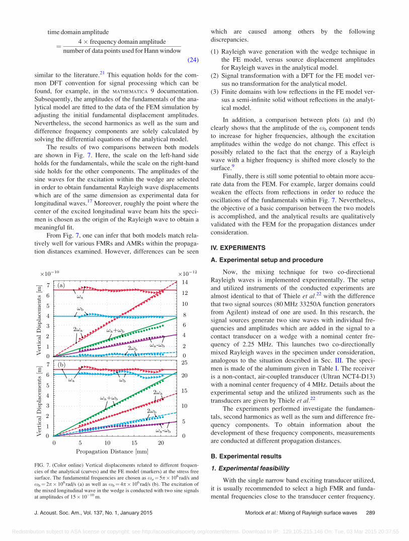
The results of two comparisons between both models
are shown in Fig. 7. Here, the scale on the left-hand side
holds for the fundamentals, while the scale on the right-hand
side holds for the other components. The amplitudes of the
sine waves for the excitation within the wedge are selected
in order to obtain fundamental Rayleigh wave displacements
which are of the same dimension as experimental data for
longitudinal waves.17 Moreover, roughly the point where the
center of the excited longitudinal wave beam hits the speci-
men is chosen as the origin of the Rayleigh wave to obtain a
meaningful fit.
From Fig. 7, one can infer that both models match rela-
tively well for various FMRs and AMRs within the propaga-
tion distances examined. However, differences can be seen
which are caused among others by the following
discrepancies.
(1) Rayleigh wave generation with the wedge technique in
the FE model, versus source displacement amplitudes
for Rayleigh waves in the analytical model.
(2) Signal transformation with a DFT for the FE model ver-
sus no transformation for the analytical model.
(3) Finite domains with low reflections in the FE model ver-
sus a semi-infinite solid without reflections in the analyt-
ical model.
In addition, a comparison between plots (a) and (b)
clearly shows that the amplitude of the xb component tends
to increase for higher frequencies, although the excitation
amplitudes within the wedge do not change. This effect is
possibly related to the fact that the energy of a Rayleigh
wave with a higher frequency is shifted more closely to the
surface.9
Finally, there is still some potential to obtain more accu-
rate data from the FEM. For example, larger domains could
weaken the effects from reflections in order to reduce the
oscillations of the fundamentals within Fig. 7. Nevertheless,
the objective of a basic comparison between the two models
is accomplished, and the analytical results are qualitatively
validated with the FEM for the propagation distances under
consideration.
IV. EXPERIMENTS
A. Experimental setup and procedure
Now, the mixing technique for two co-directional
Rayleigh waves is implemented experimentally. The setup
and utilized instruments of the conducted experiments are
almost identical to that of Thiele et al.22 with the difference
that two signal sources (80 MHz 33250A function generators
from Agilent) instead of one are used. In this research, the
signal sources generate two sine waves with individual fre-
quencies and amplitudes which are added in the signal to a
contact transducer on a wedge with a nominal center fre-
quency of 2.25 MHz. This launches two co-directionally
mixed Rayleigh waves in the specimen under consideration,
analogous to the situation described in Sec. III. The speci-
men is made of the aluminum given in Table I. The receiver
is a non-contact, air-coupled transducer (Ultran NCT4-D13)
with a nominal center frequency of 4 MHz. Details about the
experimental setup and the utilized instruments such as the
transducers are given by Thiele et al.22
The experiments performed investigate the fundamen-
tals, second harmonics as well as the sum and difference fre-
quency components. To obtain information about the
development of these frequency components, measurements
are conducted at different propagation distances.
B. Experimental results
1. Experimental feasibility
With the single narrow band exciting transducer utilized,
it is usually recommended to select a high FMR and funda-
mental frequencies close to the transducer center frequency.
FIG. 7. (Color online) Vertical displacements related to different frequen-
cies of the analytical (curves) and the FE model (markers) at the stress free
surface. The fundamental frequencies are chosen as xa¼ 5p� 106 rad/s and
xb¼ 2p� 106 rad/s (a) as well as xb¼ 4p� 106 rad/s (b). The excitation of
the mixed longitudinal wave in the wedge is conducted with two sine signals
at amplitudes of 15� 10�10 m.
J. Acoust. Soc. Am., Vol. 137, No. 1, January 2015 Morlock et al.: Mixing of Rayleigh surface waves 289
Redistribution subject to ASA license or copyright; see http://acousticalsociety.org/content/terms. Download to IP: 129.105.215.146 On: Tue, 03 Mar 2015 20:37:55

Nevertheless, the FMR should not be too close to a value of
one in order to avoid overlaps between the frequency
components considered in the DFT. Thus, the fundamental
frequencies of Sec. II E 2 which are fa¼ 2.333333 MHz and
fb¼ 1.866667 MHz are used for all following experiments
[with f¼x/(2p)]. In addition, as it was not possible to mea-
sure meaningful data for the difference frequency component
with the present setup due to bandwidth limitations of the
receiving transducer, the experiments focus solely on the fun-
damentals, second harmonics and the sum frequency
component.
The procedure for the data processing is similar to Thiele
et al.22 Initially, a time domain signal is measured at the cen-
ter of the wave beam. Based on this, a Hann window and the
DFT lead to a frequency domain representation such as in
Fig. 8, where the amplitudes have been back calculated to the
time domain with Eq. (24). Note that the utilized air-coupled
transducer measures the amplitude of the leaked longitudinal
wave in the air in volts which is approximately proportional
to the particle displacements in the material and will therefore
be used in the same sense throughout this section. In addition,
the maxima of the frequency components considered in Fig. 8
cannot be directly compared to each other because of the fre-
quency response of the receiving transducer.
As a next step, these maxima are determined at propaga-
tion distances from 30 to 78 mm in 1 mm increments, which
yields Fig. 9. Here, some typical characteristics can be
observed—the fundamentals transfer their energy to the
other frequency components and get attenuated as well as
diffracted leading to a decrease in amplitude. In contrast, the
second harmonics and the sum frequency component rise
essentially. However, as the measurements are conducted in
the far field, attenuation as well as diffraction effects tend to
significantly decrease the wave generation of these compo-
nents at larger propagation distances.
Subsequently, in Fig. 10 the ANP formulas of Eq. (22)
multiplied by x are used. At this, the measured amplitudes in
volts are representatively used for the displacement ampli-
tudes, which only gives relative ANPs. In addition, the scale
on the right-hand side solely holds for b11 and for the quali-
tative investigations of this research, only one set of meas-
urements is conducted because of the high repeatability.22
Thiele et al.22 used the same propagation distances and
a similar fundamental frequency to examine second har-
monic generation with a single fundamental, where they
observed a relatively constant behavior for the ANP. Also, it
can be inferred from the simulations of Fig. 5, where the
attenuation coefficient of the xa component and the frequen-
cies of the experiment have been used, that the behavior of
the three considered ANPs should also be approximately
constant for the propagation distances under consideration.
Note that as the initial fundamental amplitudes in the analyt-
ical investigations could be relatively different from the
experiments, the simulations are supposed to be only utilized
as an orientation. Nevertheless, useful measurements should
allow for acceptable linear fits with the different ANPs as
FIG. 8. (Color online) DFT of the time domain signal measured at 78 mm
propagation distance with a Hann window applied to a steady state portion.
Both function generator outputs are set to 700 mVpp. [Note, for example,
that fa¼xa /(2p), etc.]
FIG. 9. (Color online) Amplitudes of different frequency components over
the propagation distance normalized to their value at 30 mm. Both function
generator outputs are set to 700 mVpp.
FIG. 10. (Color online) Different ANPs times propagation distance x for ex-
perimental data (markers). The slopes of the corresponding linear fits (lines)
and the standard errors (SE) in m2/(Vmm) are specified. Both function gen-
erator outputs are set to 700 mVpp.
290 J. Acoust. Soc. Am., Vol. 137, No. 1, January 2015 Morlock et al.: Mixing of Rayleigh surface waves
Redistribution subject to ASA license or copyright; see http://acousticalsociety.org/content/terms. Download to IP: 129.105.215.146 On: Tue, 03 Mar 2015 20:37:55

corresponding slopes. In fact, the linear fits within Fig. 10
are reasonable.
Thus, it can be concluded that co-directional Rayleigh
wave mixing is experimentally feasible in order to obtain a
meaningful relative measure of the acoustic nonlinearity of a
material in at least three different ways.
2. Variation of initial fundamental amplitudes
Finally, a set of ultrasonic measurements is performed to
determine if the theory is in accordance with the behavior of
the experimental setup for variations of the output voltage of
the function generators. A range from 300 to 700 mVpp is
selected for which the overall setup behaves relatively
linearly. Thus, the initial fundamental amplitudes are approxi-
mately proportional to the output voltage of the corresponding
function generator. One set of measurements is conducted for
each combination of output voltages for propagation distances
from 30 to 78 mm at increments of 4 mm.
In Fig. 11 the results of the average amplitudes over the
propagation distance of the second harmonics and the sum
frequency component are shown. The second harmonics
scale approximately with the square of the corresponding
initial fundamental amplitude, and function generator output
voltage, respectively. The sum frequency component
increases nearly linearly, but in both axis directions.
The experimental dependence of the second harmonics
and the sum frequency component on the initial fundamental
amplitudes is similarly predicted by theoretical investiga-
tions—for example, by the quasilinear theory for a Gaussian
source of Shull et al.12 when applied to the problem under
consideration, or by Eq. (17) for small propagation distances.
V. CONCLUSION
This paper demonstrates a variety of effects and possi-
bilities concerning the mixing of two co-directional
Rayleigh waves in a weakly nonlinear solid by using analyti-
cal models, FEM simulations and experiments.
First, the existing nonlinear theory for a single funda-
mental Rayleigh wave9,12 is extended to the case of co-
directional mixing of two Rayleigh waves. Simulation mod-
els are developed which incorporate interaction as well as
attenuation and diffraction effects. Shock plus pulse forma-
tions in the waveforms of the particle velocities and the de-
velopment of the displacement amplitudes of the
fundamentals, second harmonics, as well as of the sum and
difference frequency components as a function of the propa-
gation distance are investigated. General recommendations
on the choice of the mixing parameters (FMR and AMR) in
order to maximize the second harmonics as well as the sum
and difference frequency components are given. Also, an im-
portant advantage of the difference frequency component
when compared to the second harmonic of a single funda-
mental wave is discussed. Furthermore, ANPs for the second
harmonics as well as for the sum and difference frequency
components are formulated, and related to each other in
order to specify the same ANP in four different ways.
Moreover, a basic version of the analytical model is
validated with a FEM simulation. In the end, experiments
show that meaningful data for the ANPs related to the sec-
ond harmonics and the sum frequency component can be
measured for co-directional Rayleigh wave mixing. This
allows the monitoring of the material state in different ways
which can be beneficial.
A next step is to confirm the proposed experimental
mixing technique with a study using different materials and
specimens.
ACKNOWLEDGMENTS
This research was performed using funding received
from the DOE Office of Nuclear Energy’s Nuclear Energy
University Programs and NST through CMMI-1363221 and
CMMI-1362204. The German Academic Exchange Service
(DAAD) and the Friedrich-Ebert-Foundation (FES) supported
this work through fellowships to M.B.M. The authors want to
thank Sebastian Thiele who installed the experimental setup.
1J. H. Cantrell, “Substructural organization, dislocation plasticity and har-
monic generation in cyclically stressed wavy slip metals,” Proc. R. Soc.
London, Ser. A 460, 757–780 (2004).2J.-Y. Kim, L. J. Jacobs, J. Qu, and J. W. Littles, “Experimental characteri-
zation of fatigue damage in a nickel-base superalloy using nonlinear ultra-
sonic waves,” J. Acoust. Soc. Am. 120, 1266–1273 (2006).3M. Liu, G. Tang, L. J. Jacobs, and J. Qu, “Measuring acoustic nonlinearity
parameter using collinear wave mixing,” J. Appl. Phys. 112, 024908
(2012).4A. J. Croxford, P. D. Wilcox, B. W. Drinkwater, and P. B. Nagy, “The use
of non-collinear mixing for nonlinear ultrasonic detection of plasticity and
fatigue,” J. Acoust. Soc. Am. 126, EL117–EL122 (2009).5G. L. Jones and D. R. Kobett, “Interaction of elastic waves in an isotropic
solid,” J. Acoust. Soc. Am. 35, 5–10 (1963).6J. Herrmann, J.-Y. Kim, L. J. Jacobs, J. Qu, J. W. Littles, and M. F.
Savage, “Assessment of material damage in a nickel-base superalloy using
nonlinear Rayleigh surface waves,” J. Appl. Phys. 99, 124913 (2006).7S. V. Walker, J.-Y. Kim, J. Qu, and L. J. Jacobs, “Fatigue damage evalua-
tion in A36 steel using nonlinear Rayleigh surface waves,” NDT&E Int.
48, 10–15 (2012).8N. Kalayanasundaram, “Nonlinear mode coupling of surface acoustic
waves on an isotropic solid,” Int. J. Eng. Sci. 19, 435–441 (1981).9E. A. Zabolotskaya, “Nonlinear propagation of plane and circular
Rayleigh waves in isotropic solids,” J. Acoust. Soc. Am. 91, 2569–2575
(1992).10E. A. Zabolotskaya, “Nonlinear propagation of Rayleigh waves,” Opt.
Acoust. Rev. 1, 133–140 (1990).11N. Kalyanasundaram, “Coupled amplitude theory of nonlinear surface
acoustic waves,” J. Acoust. Soc. Am. 72, 488–493 (1982).
FIG. 11. (Color online) Average amplitudes normalized to the maximum of
the corresponding frequency component for different output voltages of the
function generators.
J. Acoust. Soc. Am., Vol. 137, No. 1, January 2015 Morlock et al.: Mixing of Rayleigh surface waves 291
Redistribution subject to ASA license or copyright; see http://acousticalsociety.org/content/terms. Download to IP: 129.105.215.146 On: Tue, 03 Mar 2015 20:37:55

12D. J. Shull, E. E. Kim, M. F. Hamilton, and E. A. Zabolotskaya,
“Diffraction effects in nonlinear Rayleigh wave beams,” J. Acoust. Soc.
Am. 97, 2126–2137 (1995).13J. H. Cantrell and T. Kundu, Ultrasonic Nondestructive Evaluation:
Engineering and Biological Material Characterization - Fundamentalsand Applications of Nonlinear Ultrasonic Nondestructive Evaluation(CRC Press, Boca Raton, FL, 2003), pp. 363–433.
14R. Bonifacio, R. Caloi, and C. Maroli, “The slowly varying envelope
approximation revisited,” Opt. Commun. 101, 185–187 (1993).15R. N. Thurston, “Interpretation of ultrasonic experiments on finite-
amplitude waves,” J. Acoust. Soc. Am. 41, 1112–1125 (1967).16D. J. Shull, M. F. Hamilton, Y. A. II’insky, and E. A. Zabolotskaya,
“Harmonic generation in plane and cylindrical nonlinear Rayleigh waves,”
J. Acoust. Soc. Am. 94, 418–427 (1993).17D. J. Barnard, “Variation of nonlinearity parameter at low fundamental
amplitudes,” Appl. Phys. Lett. 74, 2447–2449 (1999).
18Y. V. Kopylov, A. V. Popov, and A. V. Vinogradov, “Application of the
parabolic wave equation to x-ray diffraction optics,” Opt. Commun. 118,
619–636 (1995).19D. M. Stobbe, “Acoustoelasticity in 7075-T651 aluminum and dependence
of third order elastic constants on fatigue damage,” Master’s thesis,
Georgia Institute of Technology, Atlanta, GA, 2005.20J.-Y. Kim, L. J. Jacobs, J. Qu, and T. Kundu, Ultrasonic and
Electromagnetic NDE for Structure and Material Characterization:Engineering and Biomedical Applications—Material Characterization byNonlinear Ultrasonic Technique (CRC Press, Boca Raton, FL, 2012), pp.
395–456.21A. Girgis and F. Ham, “A quantitative study of pitfalls in the FFT,” IEEE
Trans. Aero. Electr. Syst. AES-16, 434–439 (1980).22S. Thiele, J.-Y. Kim, J. Qu, and L. J. Jacobs, “Air-coupled detection of
nonlinear Rayleigh surface waves to assess material nonlinearity,”
Ultrasonics 54, 1470–1475 (2014).
292 J. Acoust. Soc. Am., Vol. 137, No. 1, January 2015 Morlock et al.: Mixing of Rayleigh surface waves
Redistribution subject to ASA license or copyright; see http://acousticalsociety.org/content/terms. Download to IP: 129.105.215.146 On: Tue, 03 Mar 2015 20:37:55