Mixing Measurements on an Equatorial Ocean...

Mixing Measurements on an Equatorial Ocean Mooring

J. N. MOUM AND J. D. NASH

College of Oceanic and Atmospheric Sciences, Oregon State University, Corvallis, Oregon

(Manuscript received 20 December 2007, in final form 9 April 2008)

ABSTRACT

Vaned, internally recording instruments that measure temperature fluctuations using FP07 thermistors,

including fluctuations in the turbulence wavenumber band, have been built, tested, and deployed on a

Tropical Atmosphere Ocean (TAO) mooring at 08, 1408W. These were supplemented with motion packages

that measure linear accelerations, from which an assessment of cable displacement and speed was made.

Motions due to vortex-induced vibrations caused by interaction of the mean flow with the cable are small

(rms , 0.15 cable diameters) and unlikely to affect estimates of the temperature variance dissipation rate xT.

Surface wave–induced cable motions are significant, commonly resulting in vertical displacements of 61 m

and vertical speeds of 60.5 m s21 on 2–10-s periods. These motions produce an enhancement to the mea-

surement of temperature gradient in the surface wave band herein that is equal to the product of the vertical

cable speed and the vertical temperature gradient (i.e., dT/dt ; wcdT/dz). However, the temperature gradient

spectrum is largely unaltered at higher and lower frequencies; in particular, there exists a clear scale sepa-

ration between frequencies contaminated by surface waves and the turbulence subrange. The effect of cable

motions on spectral estimates of xT is evaluated and determined to result in acceptably small uncertainties

(, a factor of two 95% of the time, based on 60-s averages). Time series of xT and the inferred turbulent

kinetic energy dissipation rate e are consistent with historical data from the same equatorial location.

1. Motivation

The need for extended observations of mixing is

highlighted by the potentially prominent role played by

mixing in changing equatorial SST on interannual (El

Nino) time scales. Coincident with the passage of a

downwelling Kelvin wave observed prior to the 1991–93

El Nino, reduced mixing observed by Lien et al. (1995)

may have provided positive feedback toward increasing

SST in the central Pacific. At the other extreme, en-

hanced subsurface mixing is a prime (but unproven)

candidate for the 88C surface cooling (in 1 month) at 0

1258W to abruptly conclude the strong 1997–98 El Nino

(McPhaden 1999; Wang and McPhaden 2001). This

enhanced mixing, inferred from bulk estimates, must

also be highly intermittent (characteristic of naturally

occurring turbulence) and not amenable to observation

from shipboard campaigns, which are infrequent, of

necessarily short duration, and must be planned years in

advance. This is exemplified by three experiments to

examine the nature of turbulent mixing in the central

equatorial Pacific: in 1984, TROPIC HEAT (Moum and

Caldwell 1989); in 1987, TROPIC HEAT 2 (Moum

et al. 1992a); and in 1991, the Tropical Instability Wave

Experiment (TIWE; Lien et al. 1995). All of these ex-

periments focused on the site at 08, 1408W, largely be-

cause of the presence of long-term moored observations

predating the full implementation of the Tropical Ocean

and Global Atmosphere–Tropical Atmosphere Ocean

(TOGA–TAO) equatorial array of moorings (McPhaden

1993). The sum duration of these intensive profiling ob-

servations was about 100 days over a period of 7 yr, with

none since 1991. Moreover, mixing parameterizations

based on these experiments have not been particularly

successful (Zaron and Moum 2008, manuscript submitted

to J. Phys. Oceanogr.). Reliably establishing the role of

mixing in interannual climate phenomena such as El

Nino is impossible without longer-term records.

To progress toward the goal of establishing extended

observations of mixing and internal gravity waves, we

have developed, tested, and deployed a string of

moored temperature microstructure recorders (xpods;

Fig. 1) at the 08, 1408W TAO mooring site. The initial

Corresponding author address: J. N. Moum, College of Oceanic

and Atmospheric Sciences, Oregon State University, COAS Ad-

min. Bldg. 104, Corvallis, OR 97331–5503.

E-mail: [email protected]

FEBRUARY 2009 M O U M A N D N A S H 317

DOI: 10.1175/2008JTECHO617.1

� 2009 American Meteorological Society

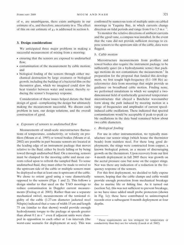
FIG. 1. (a) xpod attached to cable over the dock in Yaquina Bay for testing, (b) a closer look

at the cable attachment, and (c) close-up of thermistor sting with protector. The diameter of the

protective ring is 18 mm. The thermistor bead is set back 4 mm from the leading edge of

the ring.

318 J O U R N A L O F A T M O S P H E R I C A N D O C E A N I C T E C H N O L O G Y VOLUME 26

deployment yielded a highly resolved, 4-month time

series of temperature T, the rate of dissipation of tem-

perature gradient fluctuations xT, the turbulent kinetic

energy dissipation rate e, and the turbulence diffusion

coefficient KT at three depths over the range 30–90 m.

We have since attempted to maintain a presence at 08,

1408W and have deployed xpods at three to six depths

continually since September 2005.

Our objective is to provide a simple, reliable, and

affordable device that can be readily integrated into

existing moorings or autonomous vehicles. We expect

these measurements will provide a meaningful begin-

ning toward the objectives of dynamically linking the

mixing to the larger spatial scales and longer time scales

at this and other locations.

In this paper, we describe the basic configuration and

philosophy behind xpod, some of the lessons we have

learned from our first deployment, and some prelimi-

nary results. We begin with a set of definitions and our

procedure for estimating xT (section 2), followed by a

summary of design considerations (section 3). The

configuration of xpod is discussed in section 4. We then

present some basic results, including measurements of

the cable motion (section 5). The effect of cable motion

is critical to our estimate of xT and is discussed in sec-

tion 6. This is followed by a comparison to historical

data (section 7) and, finally, a summary and conclusions

(section 8).

2. Definitions and procedures

a. xT, e, and KT

The ultimate objective of these mixing measurements

is the computation of xT, e, KT, the turbulent heat and

buoyancy fluxes KT dT/dz and N2KT, and their vertical

divergences. Here, N2 5 2g/r � dr/dz is the squared

buoyancy frequency, g is the acceleration due to gravity,

and r is density.

With fully resolved measurements of =T in the dif-

fusive subrange of turbulence, the dissipation rate of

temperature variance can be computed as

xT 5 2DTdT

dxi

dT

dxi

� �; ð1Þ

which for isotropic turbulence becomes

xT 5 6DTdT

dx

dT

dx

� �5 6DT

ð‘

0

CTxðkÞdk; ð2Þ

where dT/dx is the alongpath (not necessarily horizontal

at all wavenumbers) component of temperature gradi-

ent, DT the thermal diffusivity, and CTxðkÞ the wave-

number spectrum of dT/dx. The brackets ideally refer to

an ensemble average; in this particular case, they refer

to a time average. We do not measure dT/dx directly;

rather, we infer it from the measured time derivative

dT/dt via Taylor’s frozen flow hypothesis

dT

dx5

1

u

dT

dt; ð3Þ

where u represents the flow speed past the thermistor.

Following Osborn and Cox (1972), the eddy diffusivity

is defined through the turbulent temperature variance

equation, assuming isotropic turbulence acts on a

background state with the only mean gradient in the

vertical coordinate direction, dT/dz. From this, the eddy

diffusivity for heat is

KT 512 xT

dT=dzh i2: ð4Þ

The wavenumber extent of CTxdepends on e through

the Batchelor wavenumber kb 5 e= nD2T

� �� 1= 4: Because

thermistors typically capture a small fraction of tem-

perature gradient variance (Lueck et al. 1977; Nash

et al. 1999), kb must be estimated to determine xT from

partially resolved spectra. In the absence of direct

measurement of the microscale velocity shear, we make

the assumption that Kr 5 KT to determine e and hence

kb (i.e., Alford and Pinkel 2000). Here,

Kr 5 Ge=N2 ð5Þ

is defined assuming a steady-state balance between

shear production, turbulence energy dissipation, and

buoyancy production Jb, with a constant mixing effi-

ciency G setting the ratio between e and Jb (Osborn

1980). Assuming the equality of Eqs. (4) and (5),

ex 5N2xT

2G dT=dzh i2; ð6Þ

where ex denotes e computed from xT.

b. Estimating xT

Because flow speeds are typically large (and variable)

and computations are made over short time intervals

(for reasons discussed in section 6), gradient spectra

contain only a small fraction of the diffusive subrange at

moderate dissipation rates, with the highest wavenumb-

ers almost always attenuated because of sensor re-

sponse. As a result, individual spectra seldom look like

the canonical Batchelor (1959) form, so curve-fitting

procedures (e.g., Luketina and Imberger 2000) fail to be

robust. In contrast, the procedure we use is insensitive

to the shape of the temperature gradient spectrum and

in no way requires that the diffusive roll-off be resolved.


Our procedure does require G; however, the depen-

dence on it is weak (see appendix).

To estimate xT when the spectrum is incompletely

resolved requires fitting observed spectra over limited

bandwidth to an accepted universal form. In practice,

we determine xT by integrating CTxðkÞ over a subrange

kmin , k , kmax that is resolved by the thermistor.

Because the frequency-response transfer functions we

determine for each thermistor (see section 4) are nei-

ther perfect nor do they extend to kb for high e and u, we

account for variance not resolved by the probe by as-

suming a universal form for the scalar spectrum at un-

resolved wavenumbers. The variance between the

measured CTxðkÞ½ �obs and theoretical CTx

ðkÞ½ �theory

spectra at resolved wavenumbers is assumed to be

equal:

ðkmax

kmin

CTxðkÞ½ �obsdk 5

ðkmax

kmin

CTxðkÞ½ �theorydk: ð7Þ

Then xT is computed from the full integral of the the-

oretical spectrum. Theoretical forms for the scalar

spectra have been proposed by Batchelor (1959) and

Kraichnan (1968). It has been found that Kraichnan’s

universal form more closely matches both field obser-

vations (Nash and Moum 2002) and fully resolved tur-

bulence simulations (Smyth 1999). We use the

Kraichnan form here but note that this choice has little

quantitative effect on our results.

The wavenumber extent of the theoretical scalar

gradient spectrum depends on the value of the universal

constant q and the Batchelor wavenumber, which we

estimate through Eq. (6) as kb5 ex= nD2T

� �� 1=4: We use

an iterative procedure to determine xT and ex that is

consistent with Eqs. (2), (6), and (7) for nominal values

of G(0.2) and q(7), initial values of kmin and kmax, and

measured values of N2, dT/dz, and CTx. The procedure

is as follows: First we estimate xT based on an initial

guess of kb. We set kmax 5 kb/2 or to a wavenumber

equivalent to f 5 40 Hz [i.e., kmax 5 2p(40)/u], which-

ever is smaller. We then use Eq. (6) to refine our esti-

mate of kb and recompute xT using Eqs. (2) and (7).

This sequence is repeated and converges after two or

three iterations. Estimates of xT from this iterative

procedure are equivalent to the explicit formulation of

Alford and Pinkel (2000), except that we use the

Kraichnan form of the spectrum. Biases associated with

this procedure are explored in the appendix.

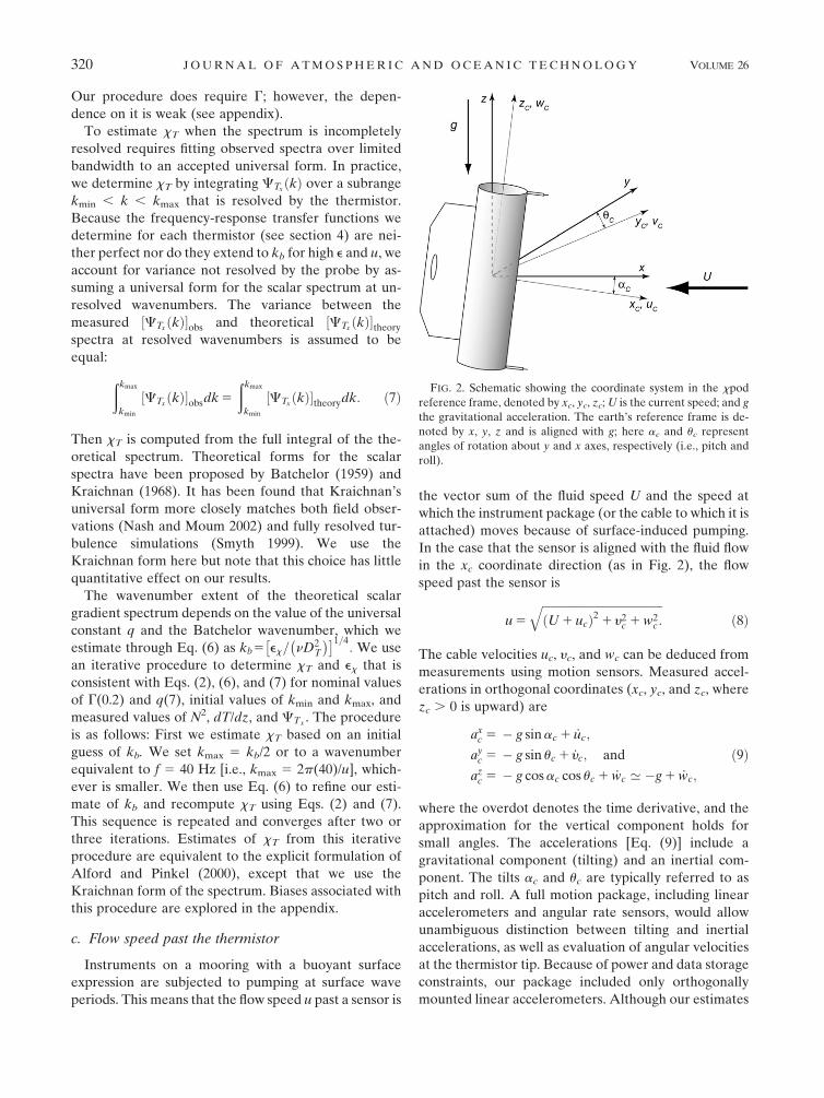
c. Flow speed past the thermistor

Instruments on a mooring with a buoyant surface

expression are subjected to pumping at surface wave

periods. This means that the flow speed u past a sensor is

the vector sum of the fluid speed U and the speed at

which the instrument package (or the cable to which it is

attached) moves because of surface-induced pumping.

In the case that the sensor is aligned with the fluid flow

in the xc coordinate direction (as in Fig. 2), the flow

speed past the sensor is

u 5

ffiffiffiffiffiffiffiffiffiffiffiffiffiffiffiffiffiffiffiffiffiffiffiffiffiffiffiffiffiffiffiffiffiffiffiffiffiffiffiffiffiffiðU 1 ucÞ2 1 y2

c 1 w2c :

qð8Þ

The cable velocities uc, yc, and wc can be deduced from

measurements using motion sensors. Measured accel-

erations in orthogonal coordinates (xc, yc, and zc, where

zc . 0 is upward) are

axc 5 � g sin ac 1 _uc;

ayc 5 � g sin uc 1 _yc; and

azc 5 � g cos ac cos uc 1 _wc ’ �g 1 _wc;

ð9Þ

where the overdot denotes the time derivative, and the

approximation for the vertical component holds for

small angles. The accelerations [Eq. (9)] include a

gravitational component (tilting) and an inertial com-

ponent. The tilts ac and uc are typically referred to as

pitch and roll. A full motion package, including linear

accelerometers and angular rate sensors, would allow

unambiguous distinction between tilting and inertial

accelerations, as well as evaluation of angular velocities

at the thermistor tip. Because of power and data storage

constraints, our package included only orthogonally

mounted linear accelerometers. Although our estimates

FIG. 2. Schematic showing the coordinate system in the xpod

reference frame, denoted by xc, yc, zc; U is the current speed; and g

the gravitational acceleration. The earth’s reference frame is de-

noted by x, y, z and is aligned with g; here ac and uc represent

angles of rotation about y and x axes, respectively (i.e., pitch and

roll).


of wc are unambiguous, there exists ambiguity in our

estimate of uc and therefore, uncertainty in u. The effect

of this on our estimate of xT is addressed in section 6.

3. Design considerations

We anticipated three major problems in making a

successful measurement of mixing from a mooring:

d ensuring that the sensors are exposed to undisturbed

flow;d contamination of the measurement by cable motion;

andd biological fouling of the sensors through either me-

chanical destruction by large creatures or biological

growth, including the buildup of a bacterial film on the

thermistor glass, which we imagined could slow the

heat transfer between water and sensor, thereby re-

ducing the sensor’s frequency response.

Consideration of these issues helped dictate the final

design of xpod—complicating the design but ultimately

making the measurement successful. We discuss each

problem in turn, our design solutions, and the overall

construction of xpod.

a. Exposure of sensors to undisturbed flow

Measurements of small-scale microstructure fluctua-

tions of temperature, conductivity, or velocity on pro-

filers (Moum et al. 1995) or towed bodies (Moum et al.

2002) are possible in part because sensors are located at

the leading edge of an instrument package that moves

relative to the fluid, either by freely falling or by being

towed through undisturbed fluid. On a mooring, sensors

must be clamped to the mooring cable and mean cur-

rents relied upon to refresh the sampled fluid. To sense

undisturbed fluid, they must either be made to swivel to

the upstream side of the cable or multiple sensors must

be deployed so that at least one is upstream of the cable.

We chose to orient xpod using a vane diametrically

opposed to the sensors (Figs. 1 and 2). This follows a

design similar to that used on the TAO moorings to

reduce contamination in Doppler current measure-

ments (Freitag et al. 2003). Rather than use a separate

mechanical swivel, measurements of the torsional ri-

gidity of the cable (1.27-cm diameter jacketed steel

Nilspin) indicated that a vane of width 15 cm and length

75 cm (similar to that shown) would provide enough

hydrodynamic torque to the package at speeds greater

than about 0.1 m s21 even if adjacent units were clam-

ped in opposition to each other at 1-m intervals (the

worst-case scenario for deployment at sea). This was

confirmed by numerous tests of multiple units on cabled

moorings in Yaquina Bay, in which currents change

direction on tidal periods and range from 0 to 1.5 m s21.

To monitor the relative directions of ambient currents

and the xpod vane, a compass was installed. In the event

that the vane did not provide sufficient steerage to ex-

pose sensors to the upstream side of the cable, data were

flagged.

b. Cable motion

Microstructure measurements from profilers and

towed bodies also require the instrument package to be

sufficiently quiet (in a hydrodynamic sense) that pack-

age motions do not contaminate the measurement.1 In

preparation for the proposal that funded this develop-

ment, we first sought high-frequency (0.1–100 Hz) ac-

celerometer data from moorings that might provide us

guidance on broadband cable motion. Finding none,

we performed simulations in which we sampled a two-

dimensional field of synthetically generated temperature

microstructure that obeyed a Batchelor wavenumber

form along the path induced by mooring motion at a

range of frequencies and amplitudes of current speed–

induced cable oscillations. These indicated that spectral

contaminations would be acceptable if peak-to-peak ca-

ble oscillations in the data band remained below about

two cable diameters.

c. Biological fouling

For use in other instrumentation, we typically man-

ufacture our sensor stings (which house the thermistor

beads) from stainless steel. For these long xpod de-

ployments, the stings were constructed from copper, a

known biological poison, as a means of discouraging

growth on the thermistors. Upon recovery from our first

4-month deployment in fall 2005 there was growth on

the acetal pressure case but none on the copper stings.

Nor was there any indication of a reduction in the fre-

quency response of the sensors.

For this first deployment, we decided to fully expose

sensors, hoping that the cable clamps and cable would

provide enough protection from mechanical breakage

due to marine life or fishing line. As it turned out

(section 5a), this was not sufficient to prevent breakage,

so we have since added small probe protectors (shown

in Fig. 1c); these have contributed to uninterrupted

records over a subsequent 8-month deployment at four

depths.

1 These requirements are less stringent for temperature or

conductivity than they are for velocity (Lueck et al. 2002).


4. Instrument configuration

Our final design included two FP07 thermistors sep-

arated by 0.9 m (for redundancy and, with both working,

to obtain a local estimate of heat flux divergence).

These were calibrated in our laboratory as a function of

temperature. For typical oceanic values of e, FP07

thermistors are not fast enough to completely resolve

the temperature variance at moderate flow speeds (i.e.,

u . 0.2 m s21). The frequency response of microbead

thermistors is unique to individual thermistors (Nash

and Moum 1999). For each thermistor, a frequency

transfer function was determined from measurements in

Yaquina Bay while mounted on our turbulence profiler

Chameleon beside a thermocouple with much faster

response (Nash et al. 1999). This, as well as a frequency

transfer function to correct for antialiasing filters, was

applied to restore lost variance to temperature gradient

spectra prior to integration to compute xT (section 2).

Error and bias associated with the response corrections

are discussed in the appendix.

The thermistors were mounted on both end caps of a

0.75-m-long, 0.1-m outside diameter pressure case con-

structed of acetal with wall thickness 0.0095 m. These

were sampled at 10 Hz and their differentiated signals

(dT/dt) at 120 Hz (Table 1). Three orthogonally ori-

ented 0–2-g linear accelerometers were sampled at 120

Hz. A compass was sampled at 1 Hz.2 A pressure sensor

ported through the lower end cap was sampled at 10 Hz.

Data were sampled as 24-bit words and the most sig-

nificant bits stored as 16-bit words. The total data rate of

631 16-bit words s21 required storage on an internal

IDE hard disk drive.3

To enable long deployments, the current load for

both analog and digital electronics was minimized. The

final design draws 24 mA average current over a 24-h

cycle. For a 6-month deployment, this requires 20 lith-

ium D-cell batteries. The pressure case is primarily a

battery pack.

5. Results from the first deployment

Three xpods were deployed by National Oceanic

and Atmospheric Administration (NOAA) personnel

aboard the R/V Ka’imimoana on the TAO mooring at 08,

1408W on 22 September 2005 and recovered on 16

January 2006. The TAO mooring configuration is dis-

cussed on NOAA’s TAO Project Web site (http://tao

.noaa.gov/). For this deployment, we purposely posi-

tioned xpods at 29, 49, and 84 m to be close to TAO

temperature sensors at 28, 48, and 80 m and TAO cur-

rent meters (Sontek Argonauts) at 25, 45, and 80 m. The

TAO temperature sensors were sampled at 10-min in-

tervals. The current data were sampled at 1 Hz and av-

eraged to 10 min before storage. A nearby subsurface

ADCP mooring provided hourly averaged currents from

3-s samples.

In this section, we discuss the temperature measure-

ments and survivability of the thermistors, as well as the

basic engineering measurements used to understand the

behavior of xpod.

a. Thermistor survivability

Measurements of temperature from the dual therm-

istors on each of three xpods are compared to nearby

TAO Sea-Bird Electronics MicroCat recorder (SBE37)

measurements on the mooring cable (Fig. 3). The upper

thermistor at 49 m was destroyed upon deployment. The

lower thermistor at 49 m shifted voltage rapidly after 3

weeks but steadied and continued to track fluctuations

in the TAO temperature measurement. The upper

thermistor at 84 m drifted slowly by 1 V after 2 weeks

and remained there for the remainder of the deploy-

ment. The lower thermistor at 84 m lasted the entire

deployment and was destroyed on recovery. The re-

maining thermistors were apparently mechanically

broken while on the mooring; the signal was lost (open

TABLE 1. xpod sensors.

Signal Sensor Manufacturer/model

Temporal

resolution

Signal

resolution

Sample rate

(Hz)

Pressure Piezoresistor Measurement Specialties 86 (0–100 psi) 0.1% FSO 10

Linear acceleration Piezoresistor IC Sensors 3052 (0–2g) 0–250 Hz 0.5% FSO 120

Compass direction Magneto-inductive Precision Navigation,

Inc. V2Xe (now using

Honeywell HMC6352)

,18 1

Temperature Thermistor GE/Thermometrics FP07 Variable nominal

3 db, 20–30 Hz

,100 mK 10

dT/dt Thermistor GE/Thermometrics 120

2 We have since switched from a Precision Navigation, Inc.

model V2Xe compass to a more reliable and higher-resolution

Honeywell HMC6352.3 We expect that continued expanded capacity of flash cards and

reduction in our data sampling will enable storage on compact

flash.


circuit voltage) between successive 10-Hz samples. The

upper thermistor at 29 m broke in mid-November and

the remaining two sensors (at 29 and 49 m) broke within

5 min of each other on 25 November. There was no

evidence of fishing line entangled in any of the mooring

gear recovered in January 2006. We suspect that

schooling fish caused the breakage. Subsequent designs

incorporate a protective copper housing to help prevent

mechanical breakage of the tip (Fig. 2c). These have

contributed to 80% data recovery in the August 2006–

May 2007 deployment. With this configuration, and the

dimensions noted in Fig. 2c, we do not expect there to

be any contamination when the flow remains aligned

within 6458 of head-on.

The temperature measurements shown were derived

from our laboratory calibrations of thermistors. Aside

from the drift at 49 m (Fig. 3c) that we cannot account

for because the sensor was later broken, our calibrations

agree to within 0.18C of the TAO temperature mea-

surements. The temperature difference (dT 5 Txpod 2

TTAO) and its variability can be attributed to the local

temperature gradient and its temporal variations. Both

the magnitude and variability in dT are largest at 84 m

for two reasons. First, the separation between sensors is

largest there: 4-m separation at 84 m compared to 1-m

separation at 29 and 49 m. Second, both dT/dz and its

variability is largest at 84 m. We note that dT is well

described by dz(dT/dz), where dz is the spacing between

sensors and dT/dz is estimated locally from Txpod using

the cable motion as described in section 5c.

b. Steering and tilts

Current speed and direction at 25-m depth are shown

in gray in Figs. 4a,b. The direction of the vane is rep-

resented by the black trace in Fig. 4b. Unfortunately,

our compass failed in mid-November. (In fact, all three

FIG. 3. (a),(c),(e) Temperature at 08, 1408W September 2005–January 2006. Plotted in gray

are temperature measurements at (a) 28, (c) 48, and (e) 80 m from SBE37 thermistors (10-min

averages reaveraged to 75 min). Red traces are derived from the upper xpod thermistors, blue

traces from the lower xpod thermistors at 29-, 49-, and 84-m depths. The data plotted are

75-min averages, which is the length of individual files written internally to xpod’s disk drive.

(b),(d),(f) Differences between xpod thermistor measurements and TAO temperature mea-

surements (dT 5 Txpod 2 TTAO).


compasses failed during the deployment; hence the

switch to a new manufacturer.) Even at relatively slow

current speeds (below 0.1 m s21) the vane was aligned

with the currents to within 208. At least on a mean basis,

the package maintains a relatively constant heading,

and the thermistors were steered into the flow to our

satisfaction.

Mean body tilts were defined from the 75-min aver-

ages of linear accelerations, via Eq. (9), with the as-

sumption that inertial accelerations do not contribute

over long time scales. Tilts were speed dependent but

limited to maxima of 138. These were not entirely re-

lated to the current speeds at 25 m because there is

strong veering of the currents in addition to direct at-

mospheric forcing on the surface float; both factors in-

fluence the shape of the cable.

c. Cable motion

The details of the motion of a point on the cable are

considerably more complex than can be discerned from

averaged data (Fig. 4). Without angular rate sensors, it

is impossible to reconstruct the details of the motion

because of the ambiguity in relative contributions of

gravitational and inertial accelerations represented by

Eq. (9); that is, we cannot tell the difference between

tilting and cable accelerations. Because knowledge of

the instantaneous speed of the fluid past the sensor is

critical to our estimate of xT, both through Eq. (3) and

in converting frequency to wavenumber for spectral

comparison to a theoretical standard, we first consider

the ranges of motions and later evaluate the conse-

quences of uncertainties in it (section 6).

FIG. 4. (a) Current speed at 25-m depth as measured from a SonTek Argonaut on the TAO

mooring. (b) Current direction from the measurement at 25-m depth (gray) and xpod direction

at 29 m (black); xpod direction is defined relative to the vane and is 1808 opposed to the

temperature sensors. (c) xpod tilts as defined in Fig. 2.


Typical acceleration spectra (Fig. 5) show the influ-

ence of surface gravity waves (at 0.1–1 Hz) and of

vortex-induced vibrations (at 5–20 Hz) in all compo-

nents and at all xpod depths; the source of the 40-Hz

signal is not clear. The effect of surface waves is largest

in the vertical component (Fig. 5c), where it is equal in

magnitude at all xpod depths. Wave signatures in the

two horizontal components (Figs. 5a,b) differ although

their magnitudes decay with increasing depth. Strouhal

frequencies (fd 5 U/5d) associated with the mean flow

(U; noted in the caption) past the cable (diameter d) are

16 Hz at 25 m, 9 Hz at 45 m, and 8 Hz at 80 m. There is

presumably broadband excitation associated with both

the range of current speeds over the upper 100 m and

the numerous other mooring components deployed

along the cable. Cable displacements at high frequen-

cies are found to be relatively small in the xc and yc

directions; rms , 2 mm over 1–45 Hz and rms , 0.1 mm

over 5–20 Hz.

For small tilts, the gravitational contribution to the

vertical acceleration is negligible, so that the vertical

speed is determined from _wc 5 azc 1 g [Eq. (9)]. This is

confirmed in Fig. 6a, which shows vertical cable velocity

spectra coincident with spectra of the time derivative of

depth (as sensed by xpod’s pressure sensor) over the

band of surface wave-induced motion; these two signals

are coherent and in phase at all depths. Vertical ex-

cursions of 61 m and vertical speeds of 60.5 m s21 at

surface wave frequencies are common and of equal

magnitude at all xpod depths. We conclude that the

vertical cable speed wc and displacement zc are reliably

determined from azc :

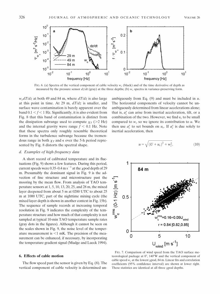
Because there is significant vertical motion in the wind

wave band that can be reliably estimated from our ac-

celerometer measurements, we test how well these cable

motions correspond to surface winds. Wind speeds mea-

sured from the surface buoy of the mooring were com-

pared to rms values of wc determined by integrating

velocity spectra over 0.1 , f , 1 Hz. This frequency band

includes both wind waves and swell (Fig. 6a), although the

vertical speed is dominated by frequencies in the wind

wave range (Fig. 6b). Surface winds and rms vertical cable

speeds are highly correlated (Fig. 7; rms values of wc and

mean values of Uwind were computed over 75-min periods

for the entire 116-day record). This suggests that im-

plementation of inexpensive and simple high-frequency

motion packages on TAO moorings may be useful for

determination of significant wave height.

One benefit of the large vertical excursions of xpod is

that we can use these to derive a robust local estimate of

dT/dz. We do this by fitting T to z over a time period

that includes at least several wave periods (in the

analysis to follow, we use 1 min).

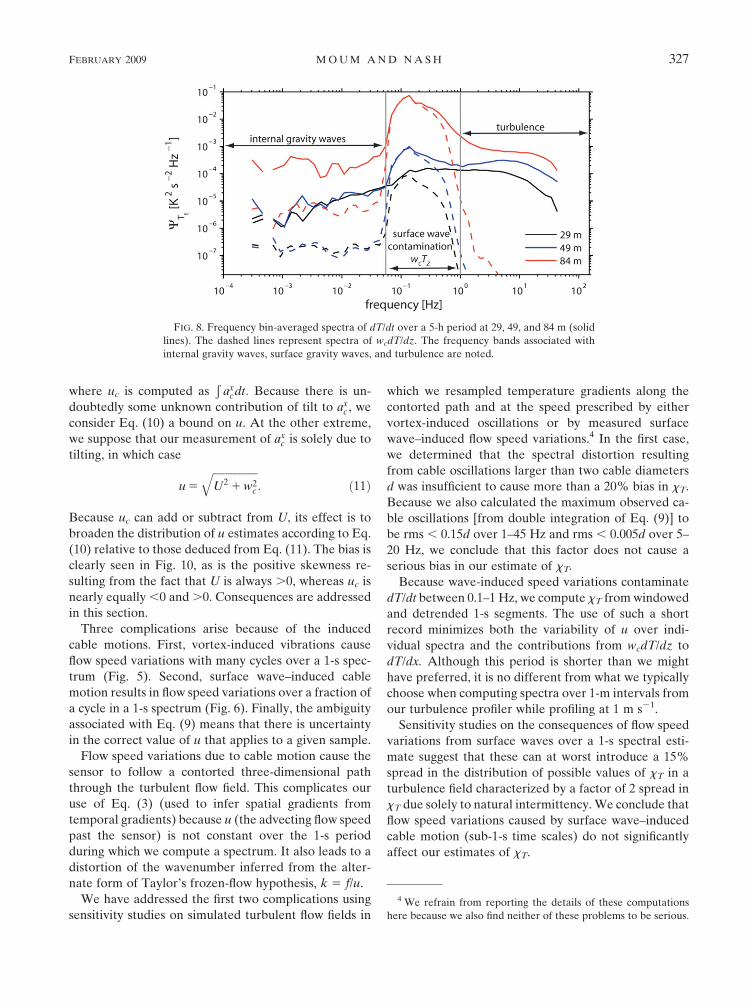
THE SPECTRUM OF dT=dt

One adverse consequence of the cable motion is that

the measured dT/dt can be dominated by vertical

pumping of the sensor through a background vertical

temperature gradient dT/dz when wc is large (Fig. 8). In

the swell data band (near 0.1 Hz), the example 5-h

spectrum of dT/dt corresponds identically with that of

FIG. 5. Acceleration spectra in the three component directions:

(a) xc, (b) yc, and (c) zc. Colors correspond to the xpod units at 29

(black), 49 (blue) and 84 m (red). These spectra were computed

from a 75-min record beginning at 2300 UTC 29 Sep 2005. Mean

current speeds over this period were 1.0 (25 m), 0.6 (45 m), and 0.5

m s21 (80 m).


wcdT/dz at both 49 and 84 m, where dT/dz is also large

at this point in time. At 29 m, dT/dz is smaller, and

surface wave contamination is barely apparent over the

band 0.1 , f , 1 Hz. Significantly, it is also evident from

Fig. 8 that this band of contamination is distinct from

the dissipation subrange used to compute xT (.2 Hz)

and the internal gravity wave range f , 0.1 Hz. Note

that these spectra only roughly resemble theoretical

forms in the turbulence subrange because the tremen-

dous range in both xT and e over the 5-h period repre-

sented by Fig. 8 distorts the spectral shape.

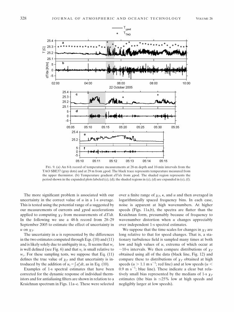
d. Examples of high-frequency data

A short record of calibrated temperature and its fluc-

tuations (Fig. 9) shows a few features. During this period,

current speeds were 0.35–0.4 m s21 at the xpod depth of 29

m. Presumably the dominant signal in Fig. 9 is the ad-

vection of fine structure and microstructure past the

mooring by the mean flow. From analysis of TAO tem-

perature sensors at 1, 5, 10, 13, 20, 25, and 28 m, the mixed

layer deepened from about 5 m at 0200 UTC to about 25

m at 1000 UTC, part of the nighttime mixing cycle (the

mixed layer depth is shown in another context in Fig. 15b).

The sequence of sample records at increasing temporal

resolution in Fig. 9 indicates the complexity of the tem-

perature structure and how much of that complexity is not

sampled at typical 10-min TAO temperature sample rates

(gray dots in the figures). Although it cannot be seen on

the scales shown in Fig. 9, the noise level of the temper-

ature measurement is ,1 mK. The precision of the mea-

surement can be enhanced, if necessary, by incorporating

the temperature gradient signal (Mudge and Lueck 1994).

6. Effects of cable motion

The flow speed past the sensor is given by Eq. (8). The

vertical component of cable velocity is determined un-

ambiguously from Eq. (9) and must be included in u.

The horizontal components of velocity cannot be un-

ambiguously determined from linear accelerations alone;

that is, axc can arise from inertial acceleration, tilt, or a

combination of the two. However, we find yc to be small

compared to wc so we ignore its contribution to u. We

then use axc to set bounds on uc. If ax

c is due solely to

inertial acceleration, then

u 5

ffiffiffiffiffiffiffiffiffiffiffiffiffiffiffiffiffiffiffiffiffiffiffiffiffiffiffiffiffiffiffiU 1 ucð Þ2 1 w2

c

q; ð10Þ

FIG. 6. (a) Spectra of the vertical component of cable velocity wc (black) and of the time derivative of depth as

measured by the pressure sensor dz/dt (gray) at the three depths; (b) wc spectra in variance-preserving form.

FIG. 7. Comparison of wind speed from the TAO surface me-

teorological package at 08, 1408W and the vertical component of

cable speed wc at the lowest xpod, 84 m. Linear fits and correlation

coefficients (95% confidence interval) are shown at lower right.

These statistics are identical at all three xpod depths.


where uc is computed asÐ

axcdt: Because there is un-

doubtedly some unknown contribution of tilt to axc , we

consider Eq. (10) a bound on u. At the other extreme,

we suppose that our measurement of axc is solely due to

tilting, in which case

u 5

ffiffiffiffiffiffiffiffiffiffiffiffiffiffiffiffiffiU2 1 w2

c

q: ð11Þ

Because uc can add or subtract from U, its effect is to

broaden the distribution of u estimates according to Eq.

(10) relative to those deduced from Eq. (11). The bias is

clearly seen in Fig. 10, as is the positive skewness re-

sulting from the fact that U is always .0, whereas uc is

nearly equally ,0 and .0. Consequences are addressed

in this section.

Three complications arise because of the induced

cable motions. First, vortex-induced vibrations cause

flow speed variations with many cycles over a 1-s spec-

trum (Fig. 5). Second, surface wave–induced cable

motion results in flow speed variations over a fraction of

a cycle in a 1-s spectrum (Fig. 6). Finally, the ambiguity

associated with Eq. (9) means that there is uncertainty

in the correct value of u that applies to a given sample.

Flow speed variations due to cable motion cause the

sensor to follow a contorted three-dimensional path

through the turbulent flow field. This complicates our

use of Eq. (3) (used to infer spatial gradients from

temporal gradients) because u (the advecting flow speed

past the sensor) is not constant over the 1-s period

during which we compute a spectrum. It also leads to a

distortion of the wavenumber inferred from the alter-

nate form of Taylor’s frozen-flow hypothesis, k 5 f/u.

We have addressed the first two complications using

sensitivity studies on simulated turbulent flow fields in

which we resampled temperature gradients along the

contorted path and at the speed prescribed by either

vortex-induced oscillations or by measured surface

wave–induced flow speed variations.4 In the first case,

we determined that the spectral distortion resulting

from cable oscillations larger than two cable diameters

d was insufficient to cause more than a 20% bias in xT.

Because we also calculated the maximum observed ca-

ble oscillations [from double integration of Eq. (9)] to

be rms , 0.15d over 1–45 Hz and rms , 0.005d over 5–

20 Hz, we conclude that this factor does not cause a

serious bias in our estimate of xT.

Because wave-induced speed variations contaminate

dT/dt between 0.1–1 Hz, we compute xT from windowed

and detrended 1-s segments. The use of such a short

record minimizes both the variability of u over indi-

vidual spectra and the contributions from wcdT/dz to

dT/dx. Although this period is shorter than we might

have preferred, it is no different from what we typically

choose when computing spectra over 1-m intervals from

our turbulence profiler while profiling at 1 m s21.

Sensitivity studies on the consequences of flow speed

variations from surface waves over a 1-s spectral esti-

mate suggest that these can at worst introduce a 15%

spread in the distribution of possible values of xT in a

turbulence field characterized by a factor of 2 spread in

xT due solely to natural intermittency. We conclude that

flow speed variations caused by surface wave–induced

cable motion (sub-1-s time scales) do not significantly

affect our estimates of xT.

FIG. 8. Frequency bin-averaged spectra of dT/dt over a 5-h period at 29, 49, and 84 m (solid

lines). The dashed lines represent spectra of wcdT/dz. The frequency bands associated with

internal gravity waves, surface gravity waves, and turbulence are noted.

4 We refrain from reporting the details of these computations

here because we also find neither of these problems to be serious.


The more significant problem is associated with our

uncertainty in the correct value of u in a 1-s average.

This is tested using the potential range of u suggested by

our measurements of currents and xpod accelerations

applied to computing xT from measurements of dT/dt.

In the following we use a 48-h record from 28–29

September 2005 to estimate the effect of uncertainty in

u on xT.

The uncertainty in u is represented by the differences

in the two estimates computed through Eqs. (10) and (11)

and is likely solely due to ambiguity in uc. It seems that wc

is well defined (see Fig. 6) and that yc is small relative to

wc. For these sampling tests, we suppose that Eq. (11)

defines the true value of xT and that uncertainty is in-

troduced by the addition of uc5Ð

axcdt, as in Eq. (10).

Examples of 1-s spectral estimates that have been

corrected for the dynamic response of individual therm-

istors and for antialiasing filters are shown in relation to a

Kraichnan spectrum in Figs. 11a–c. These were selected

over a finite range of xT, e, and u and then averaged in

logarithmically spaced frequency bins. In each case,

noise is apparent at high wavenumbers. At higher

speeds (Figs. 11a,b), the spectra are flatter than the

Kraichnan form, presumably because of frequency to

wavenumber distortion when u changes appreciably

over independent 1-s spectral estimates.

We suppose that the time scales for changes in xT are

long relative to that for speed changes. That is, a sta-

tionary turbulence field is sampled many times at both

low and high values of u, extrema of which occur at

;10-s intervals. We then compare distributions of xT

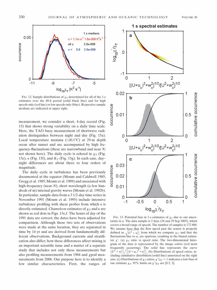
obtained using all of the data (black line, Fig. 12) and

compare these to distributions of xT obtained at high

speeds (u . 1.1 m s21; red line) and at low speeds (u ,

0.9 m s21; blue line). These indicate a clear but rela-

tively small bias represented by the medians of 1-s xT

estimates (the bias is ’25% low at high speeds and

negligibly larger at low speeds).

FIG. 9. (a) An 8-h record of temperature measurements at 28-m depth and 10-min intervals from the

TAO SBE37 (gray dots) and at 29 m from xpod. The black trace represents temperature measured from

the upper thermistor. (b) Temperature gradient dT/dx from xpod. The shaded region represents the

period shown in the expanded plots labeled (c), (d); the shaded regions in (c), (d) are expanded in (e), (f).


We now use 1-s spectral estimates of xT from the

same 48-h period to determine, on a point-to-point ba-

sis, the uncertainty in xT associated solely with our

presumed uncertainty in u. The result (Fig. 13) indicates

the uncertainty to be less than a factor of 3 95% of the

time on 1-s estimates; it is roughly predicted by the

curve U2 1 w2c

� �=½ U 1 ucð Þ2 1 w2

c �; which is how the es-

timate of xT is affected through Eq. (3).

Uncertainty is reduced considerably over a 60-s av-

erage (Fig. 14). This is due to the fact that the largest

unresolved speed fluctuations (both positive and nega-

tive) are on periods significantly less than 60 s, so these

are averaged. Presumably, the remaining (small) posi-

tive bias in xT results from the asymmetric curve in Fig.

13a. For further analysis of long time series, 60-s aver-

ages represent the base dataset.

It is very likely that short time scale variations cause

local velocity fluctuations that are unresolved in the

TAO velocity measurements. These may be due to

phenomena such as narrow band internal gravity waves,

for example, that are thought to play an important role

in equatorial mixing (Moum et al. 1992b). It is unlikely,

however, that the velocity signals of these are as large as

the cable speeds induced by surface waves.

Other sources of uncertainty in our estimates of xT

arise independently from uncertainties in the precise

form of the theoretical spectrum, the magnitude of the

mixing efficiency required to evaluate Eqs. (5) and (6),

and the cutoff frequency determined to represent the

dynamic response of individual thermistors. These are

discussed separately in the appendix.

7. Time series of xT, e, and KT and comparison tohistorical data

The purpose of this measurement is to obtain long,

uninterrupted time series of equatorial mixing. In ex-

amining the entire record of this and following de-

ployments, there appear to be many different mixing

states; this is a focus of ongoing scientific analysis. For

the purpose here of developing confidence in this new

FIG. 10. Distributions of u 5

ffiffiffiffiffiffiffiffiffiffiffiffiffiffiffiffiffiffiU2 1 w2

c

q(thick solid line), U

(thin solid line), and

ffiffiffiffiffiffiffiffiffiffiffiffiffiffiffiffiffiffiffiffiffiffiffiffiffiffiffiffiffiffiffiU 1 ucð Þ2 1 w2

c

q(dotted–dashed line) for the

48-h period of 28–29 Sep 2005 (also depicted in Figs. 11 and

12). The filled ranges at the top were used to select the data in

Fig. 11.

FIG. 11. Averaged 1-s spectra for the three filled ranges of flow

speed u shown in Fig. 10: (a) 1.2–1.4, (b) 0.9–1.1, and (c) 0.6–0.8

m s21. Data were also selected with the following requirements: 8 3

1029 , xT , 2 3 1028 K2 s21 and 7.5 3 10210 , e , 1 3 1029

m2 s23. Integration limits for the computation of xT are denoted

by the ticks on the upper axes.


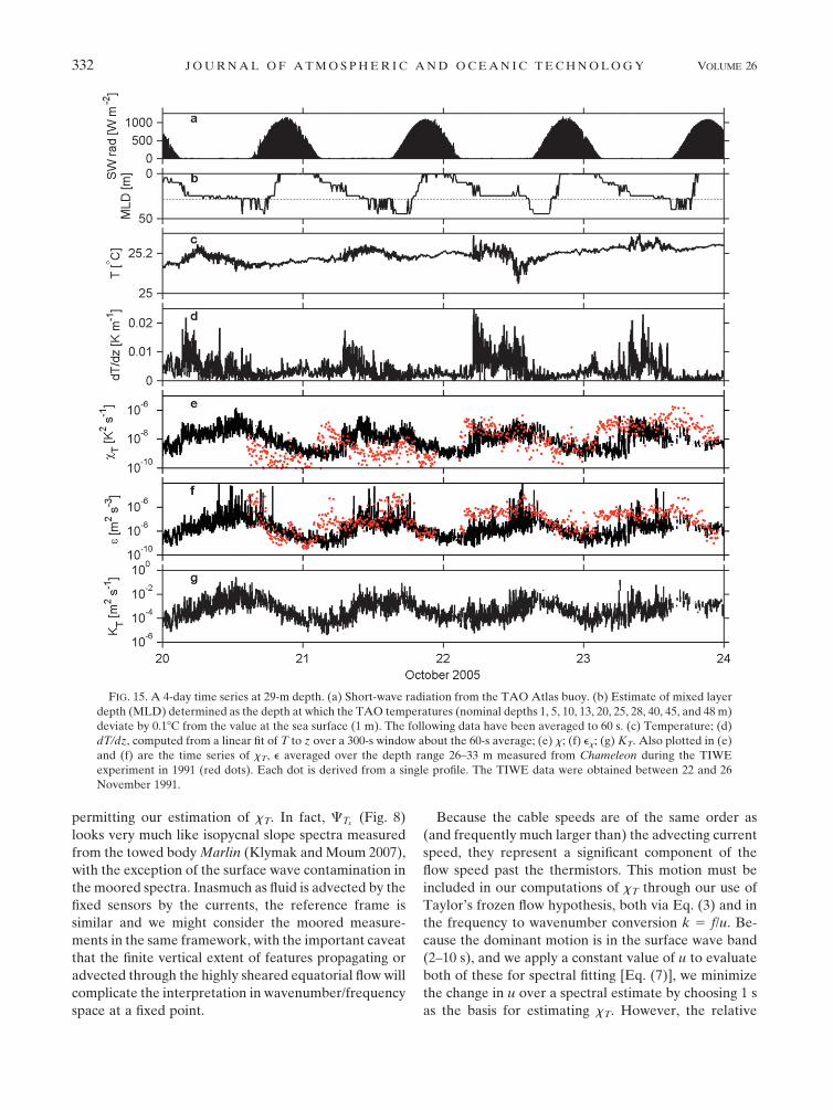
measurement, we consider a short, 4-day record (Fig.

15) that shows strong variability on a daily time scale.

Here, the TAO buoy measurement of shortwave radi-

ation distinguishes between night and day (Fig. 15a).

Local temperature maxima (’l0.18C) at 29-m depth

occur after sunset and are accompanied by high fre-

quency-fluctuations (these are narrowband and near N;

not shown here). The daily cycle is echoed in xT (Fig.

15e), e (Fig. 15f), and KT (Fig. 15g). In each case, day–

night differences are about three to four orders of

magnitude.

The daily cycle in turbulence has been previously

documented at the equator (Moum and Caldwell 1985;

Gregg et al. 1985; Moum et al. 1989) and associated with

high-frequency (near-N), short wavelength (a few hun-

dreds of m) internal gravity waves (Moum et al. 1992b).

In particular, sample data from a 3 1/2-day time series in

November 1991 (Moum et al. 1995) include intensive

turbulence profiling with shear probes from which e is

directly estimated. Chameleon estimates of xT and e are

shown as red dots in Figs. 15e,f. The hours of day of the

1991 data are correct; the dates have been adjusted for

comparision. Although these two sets of observations

were made at the same location, they are separated in

time by 14 yr and are derived from fundamentally dif-

ferent observations. Background currents and stratifi-

cation also differ; how these differences affect mixing is

an important scientific issue and a matter of a separate

study that includes not only these measurements but

also profiling measurements from 1984 and xpod mea-

surements from 2006. Our purpose here is to identify a

few similar characteristics. First, the ranges of

FIG. 12. Sample distributions of xT determined for all of the 1-s

estimates over the 48-h period (solid black line) and for high

speeds only (red line) or low speeds only (blue). Respective sample

medians are indicated at upper right.

FIG. 13. Potential bias in 1-s estimates of xT due to our uncer-

tainty in u. The data sample is 2 days (28 and 29 Sep 2005), which

covers a broad range of speeds. The number of samples is 172 800.

We assume here that the flow speed past the sensor is properly

defined asffiffiffiffiffiffiffiffiffiffiffiffiffiffiffiffiffiffiU2 1 w2

c

q; from which we compute xT, and that the

fluctuations due to uc are spurious, resulting in the biased estima-

tor x9. (a) xT ratio vs speed ratio. The two-dimensional histo-

gram of the data is represented by the image colors (red most

frequently occurring). The solid line represents the curve

U2 1 w2c

� �.U1ucð Þ21w2

c

h i. (b) Distributions of speed ratios, in-

cluding cumulative distribution (solid line) annotated on the right

axis. (c) Distributions of xT ratios; x9/xT . 1 indicates a low bias of

our estimate xT. 95% limits on x9/xT are [0.5, 3].


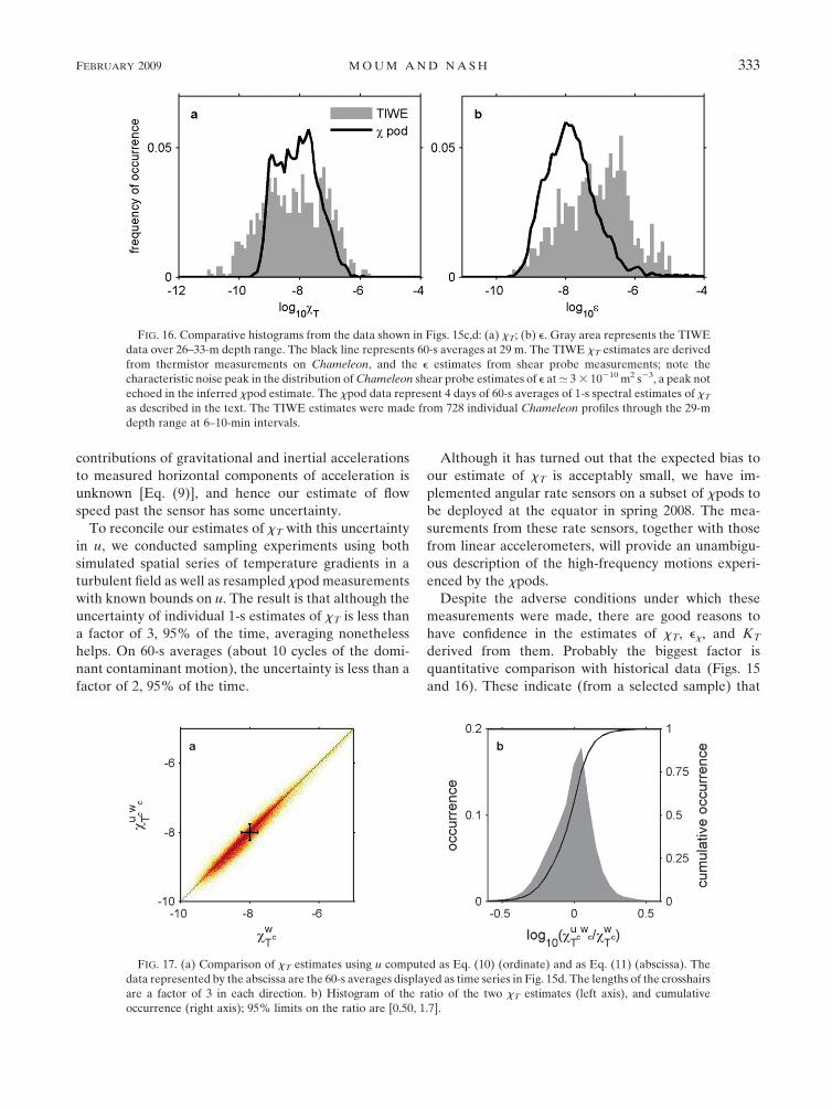
magnitudes of xT and e, although not identical, are not

very different. This is more easily seen in Fig. 16, which

shows perhaps a lower noise level in xT from the 1991

profiler measurements and a tendency to larger values

of e, which may be due to differing oceanographic

forcing of turbulence between the two measurement

periods. Second, the daytime suppression of xT and e is

in phase between the two datasets, although both the

timing and magnitude of nighttime excitation differ.

And finally, the total day/night variability is nearly the

same (three to four orders of magnitude in both xT

and e).

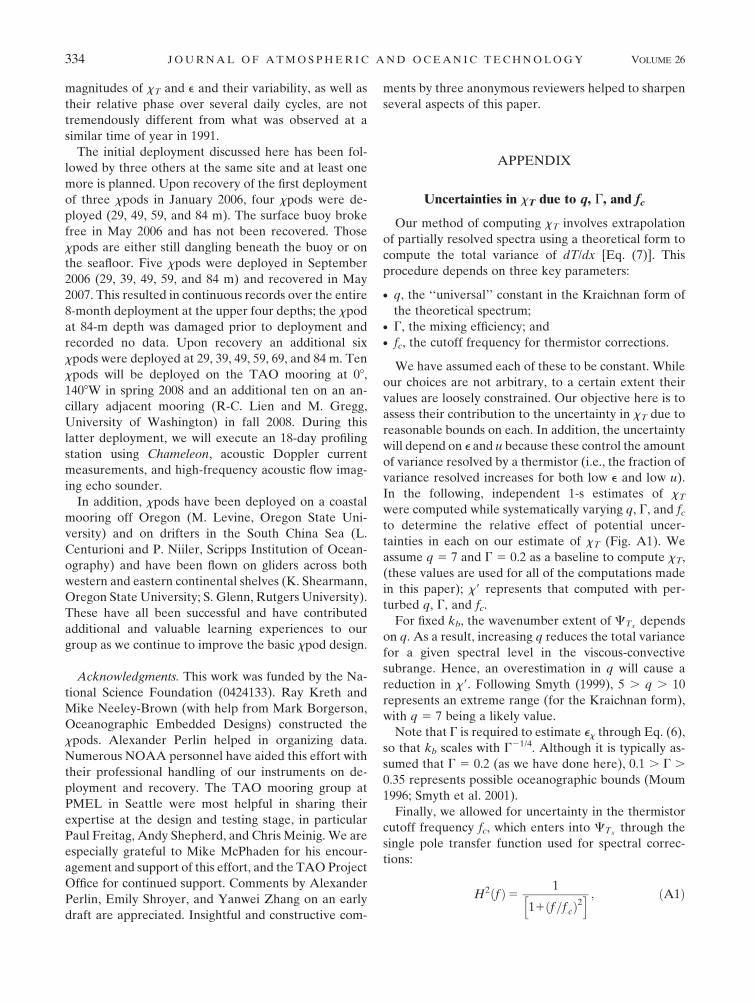
As a final sampling test on the uncertainty in xT

caused by uncertainty in u, we reconsider the xpod data

represented by Figs. 15 and 16. The entire 4-day record

was recomputed using both Eqs. (10) and (11) and the

results were summarized in Fig. 17. The result is that

95% of the values of 60-s estimates of xT are within a

factor of 2 of each other.

8. Summary and conclusions

At the design stage, we had full confidence that we

could reduce power consumption and increase data

storage sufficiently to execute long and continuous de-

ployments that included not only the basic measure-

ment of temperature and its high wavenumber gradients

but also a measure of the instrument package motion.

We were more concerned that bare thermistors would

not survive long deployments, that they would not be

reliably exposed to undisturbed flow, or that vortex-in-

duced vibrations might contaminate the measurement.

Fortunately, none of these factors have been limiting.

Although mechanical breakage of sensors on the first

deployment led to shortened records, our subsequent ad-

dition of protective rings to the sensors has resulted in

much higher data recoveries.

The use of a vane to steer the xpods has been a suc-

cessful means of keeping the sensors exposed to undis-

turbed fluid, at least at the range of current speeds

observed to date. Although vortex-induced vibrations

of the moored cable are clearly evident (Fig. 5), their

amplitudes are sufficiently small (no more than 0.15

cable diameters rms across all potentially excited fre-

quencies) that their effect on the measurement of xT is

imperceptible.

A potentially more critical problem has been the

large surface wave–induced cable motions that cause

vertical displacements of 61 m and vertical cable speeds

of 60.5 m s21 in the surface wave frequency band (2–10 s).

One of two unanticipated benefits has been that xpod

acts as a vertical profiler (at least over limited range),

yielding a robust local measure of dT/dz. Also, because

the spectral energy of wc is dominated by frequencies in

the wind wave band (Fig. 6), there exists a close corre-

lation to the surface wind speed (Fig. 7).

The vertical motion appears in the temperature gra-

dient spectrum CTxas wc dT/dz, which clearly defines

the band of frequencies contaminated by surface wave

pumping (Fig. 8). At lower frequencies, we expect in-

ternal gravity waves to dominate. At higher frequencies,

the turbulence subrange is apparently unaffected, thus

FIG. 14. As in Fig. 13, but the values are 60-s averages of the 1-s

data. Note scale changes; 95% limits on x9/xT are [0.9, 2].


permitting our estimation of xT. In fact, CTx(Fig. 8)

looks very much like isopycnal slope spectra measured

from the towed body Marlin (Klymak and Moum 2007),

with the exception of the surface wave contamination in

the moored spectra. Inasmuch as fluid is advected by the

fixed sensors by the currents, the reference frame is

similar and we might consider the moored measure-

ments in the same framework, with the important caveat

that the finite vertical extent of features propagating or

advected through the highly sheared equatorial flow will

complicate the interpretation in wavenumber/frequency

space at a fixed point.

Because the cable speeds are of the same order as

(and frequently much larger than) the advecting current

speed, they represent a significant component of the

flow speed past the thermistors. This motion must be

included in our computations of xT through our use of

Taylor’s frozen flow hypothesis, both via Eq. (3) and in

the frequency to wavenumber conversion k 5 f/u. Be-

cause the dominant motion is in the surface wave band

(2–10 s), and we apply a constant value of u to evaluate

both of these for spectral fitting [Eq. (7)], we minimize

the change in u over a spectral estimate by choosing 1 s

as the basis for estimating xT. However, the relative

FIG. 15. A 4-day time series at 29-m depth. (a) Short-wave radiation from the TAO Atlas buoy. (b) Estimate of mixed layer

depth (MLD) determined as the depth at which the TAO temperatures (nominal depths 1, 5, 10, 13, 20, 25, 28, 40, 45, and 48 m)

deviate by 0.18C from the value at the sea surface (1 m). The following data have been averaged to 60 s. (c) Temperature; (d)

dT/dz, computed from a linear fit of T to z over a 300-s window about the 60-s average; (e) x; (f) ex; (g) KT. Also plotted in (e)

and (f) are the time series of xT, e averaged over the depth range 26–33 m measured from Chameleon during the TIWE

experiment in 1991 (red dots). Each dot is derived from a single profile. The TIWE data were obtained between 22 and 26

November 1991.


contributions of gravitational and inertial accelerations

to measured horizontal components of acceleration is

unknown [Eq. (9)], and hence our estimate of flow

speed past the sensor has some uncertainty.

To reconcile our estimates of xT with this uncertainty

in u, we conducted sampling experiments using both

simulated spatial series of temperature gradients in a

turbulent field as well as resampled xpod measurements

with known bounds on u. The result is that although the

uncertainty of individual 1-s estimates of xT is less than

a factor of 3, 95% of the time, averaging nonetheless

helps. On 60-s averages (about 10 cycles of the domi-

nant contaminant motion), the uncertainty is less than a

factor of 2, 95% of the time.

Although it has turned out that the expected bias to

our estimate of xT is acceptably small, we have im-

plemented angular rate sensors on a subset of xpods to

be deployed at the equator in spring 2008. The mea-

surements from these rate sensors, together with those

from linear accelerometers, will provide an unambigu-

ous description of the high-frequency motions experi-

enced by the xpods.

Despite the adverse conditions under which these

measurements were made, there are good reasons to

have confidence in the estimates of xT, ex, and KT

derived from them. Probably the biggest factor is

quantitative comparison with historical data (Figs. 15

and 16). These indicate (from a selected sample) that

FIG. 16. Comparative histograms from the data shown in Figs. 15c,d: (a) xT; (b) e. Gray area represents the TIWE

data over 26–33-m depth range. The black line represents 60-s averages at 29 m. The TIWE xT estimates are derived

from thermistor measurements on Chameleon, and the e estimates from shear probe measurements; note the

characteristic noise peak in the distribution of Chameleon shear probe estimates of e at’ 3 3 10210 m2 s23, a peak not

echoed in the inferred xpod estimate. The xpod data represent 4 days of 60-s averages of 1-s spectral estimates of xT

as described in the text. The TIWE estimates were made from 728 individual Chameleon profiles through the 29-m

depth range at 6–10-min intervals.

FIG. 17. (a) Comparison of xT estimates using u computed as Eq. (10) (ordinate) and as Eq. (11) (abscissa). The

data represented by the abscissa are the 60-s averages displayed as time series in Fig. 15d. The lengths of the crosshairs

are a factor of 3 in each direction. b) Histogram of the ratio of the two xT estimates (left axis), and cumulative

occurrence (right axis); 95% limits on the ratio are [0.50, 1.7].


magnitudes of xT and e and their variability, as well as

their relative phase over several daily cycles, are not

tremendously different from what was observed at a

similar time of year in 1991.

The initial deployment discussed here has been fol-

lowed by three others at the same site and at least one

more is planned. Upon recovery of the first deployment

of three xpods in January 2006, four xpods were de-

ployed (29, 49, 59, and 84 m). The surface buoy broke

free in May 2006 and has not been recovered. Those

xpods are either still dangling beneath the buoy or on

the seafloor. Five xpods were deployed in September

2006 (29, 39, 49, 59, and 84 m) and recovered in May

2007. This resulted in continuous records over the entire

8-month deployment at the upper four depths; the xpod

at 84-m depth was damaged prior to deployment and

recorded no data. Upon recovery an additional six

xpods were deployed at 29, 39, 49, 59, 69, and 84 m. Ten

xpods will be deployed on the TAO mooring at 08,

1408W in spring 2008 and an additional ten on an an-

cillary adjacent mooring (R-C. Lien and M. Gregg,

University of Washington) in fall 2008. During this

latter deployment, we will execute an 18-day profiling

station using Chameleon, acoustic Doppler current

measurements, and high-frequency acoustic flow imag-

ing echo sounder.

In addition, xpods have been deployed on a coastal

mooring off Oregon (M. Levine, Oregon State Uni-

versity) and on drifters in the South China Sea (L.

Centurioni and P. Niiler, Scripps Institution of Ocean-

ography) and have been flown on gliders across both

western and eastern continental shelves (K. Shearmann,

Oregon State University; S. Glenn, Rutgers University).

These have all been successful and have contributed

additional and valuable learning experiences to our

group as we continue to improve the basic xpod design.

Acknowledgments. This work was funded by the Na-

tional Science Foundation (0424133). Ray Kreth and

Mike Neeley-Brown (with help from Mark Borgerson,

Oceanographic Embedded Designs) constructed the

xpods. Alexander Perlin helped in organizing data.

Numerous NOAA personnel have aided this effort with

their professional handling of our instruments on de-

ployment and recovery. The TAO mooring group at

PMEL in Seattle were most helpful in sharing their

expertise at the design and testing stage, in particular

Paul Freitag, Andy Shepherd, and Chris Meinig. We are

especially grateful to Mike McPhaden for his encour-

agement and support of this effort, and the TAO Project

Office for continued support. Comments by Alexander

Perlin, Emily Shroyer, and Yanwei Zhang on an early

draft are appreciated. Insightful and constructive com-

ments by three anonymous reviewers helped to sharpen

several aspects of this paper.

APPENDIX

Uncertainties in xT due to q, G, and fc

Our method of computing xT involves extrapolation

of partially resolved spectra using a theoretical form to

compute the total variance of dT/dx [Eq. (7)]. This

procedure depends on three key parameters:

d q, the ‘‘universal’’ constant in the Kraichnan form of

the theoretical spectrum;d G, the mixing efficiency; andd fc, the cutoff frequency for thermistor corrections.

We have assumed each of these to be constant. While

our choices are not arbitrary, to a certain extent their

values are loosely constrained. Our objective here is to

assess their contribution to the uncertainty in xT due to

reasonable bounds on each. In addition, the uncertainty

will depend on e and u because these control the amount

of variance resolved by a thermistor (i.e., the fraction of

variance resolved increases for both low e and low u).

In the following, independent 1-s estimates of xT

were computed while systematically varying q, G, and fc

to determine the relative effect of potential uncer-

tainties in each on our estimate of xT (Fig. A1). We

assume q 5 7 and G 5 0.2 as a baseline to compute xT,

(these values are used for all of the computations made

in this paper); x9 represents that computed with per-

turbed q, G, and fc.

For fixed kb, the wavenumber extent of CTxdepends

on q. As a result, increasing q reduces the total variance

for a given spectral level in the viscous-convective

subrange. Hence, an overestimation in q will cause a

reduction in x9. Following Smyth (1999), 5 . q . 10

represents an extreme range (for the Kraichnan form),

with q 5 7 being a likely value.

Note that G is required to estimate ex through Eq. (6),

so that kb scales with G21/4. Although it is typically as-

sumed that G 5 0.2 (as we have done here), 0.1 . G .

0.35 represents possible oceanographic bounds (Moum

1996; Smyth et al. 2001).

Finally, we allowed for uncertainty in the thermistor

cutoff frequency fc, which enters into CTxthrough the

single pole transfer function used for spectral correc-

tions:

H2 fð Þ5 1

11 f=f cð Þ2h i ; ðA1Þ


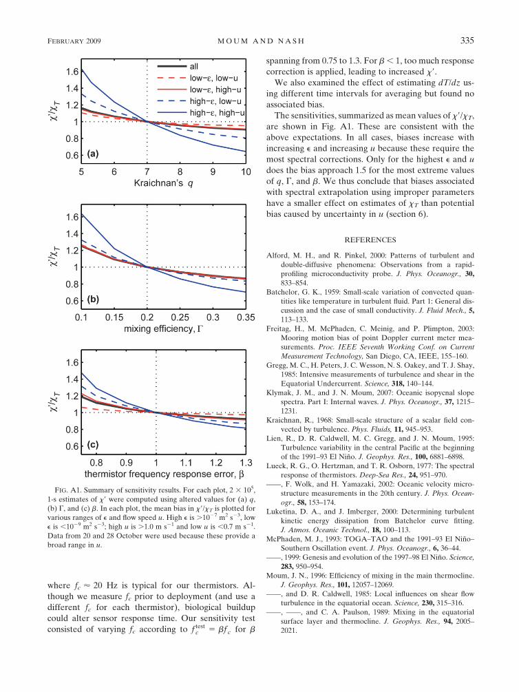
where fc ’ 20 Hz is typical for our thermistors. Al-

though we measure fc prior to deployment (and use a

different fc for each thermistor), biological buildup

could alter sensor response time. Our sensitivity test

consisted of varying fc according to f testc 5 bf c for b

spanning from 0.75 to 1.3. For b , 1, too much response

correction is applied, leading to increased x9.

We also examined the effect of estimating dT/dz us-

ing different time intervals for averaging but found no

associated bias.

The sensitivities, summarized as mean values of x9/xT,

are shown in Fig. A1. These are consistent with the

above expectations. In all cases, biases increase with

increasing e and increasing u because these require the

most spectral corrections. Only for the highest e and u

does the bias approach 1.5 for the most extreme values

of q, G, and b. We thus conclude that biases associated

with spectral extrapolation using improper parameters

have a smaller effect on estimates of xT than potential

bias caused by uncertainty in u (section 6).

REFERENCES

Alford, M. H., and R. Pinkel, 2000: Patterns of turbulent and

double-diffusive phenomena: Observations from a rapid-

profiling microconductivity probe. J. Phys. Oceanogr., 30,

833–854.

Batchelor, G. K., 1959: Small-scale variation of convected quan-

tities like temperature in turbulent fluid. Part 1: General dis-

cussion and the case of small conductivity. J. Fluid Mech., 5,

113–133.

Freitag, H., M. McPhaden, C. Meinig, and P. Plimpton, 2003:

Mooring motion bias of point Doppler current meter mea-

surements. Proc. IEEE Seventh Working Conf. on Current

Measurement Technology, San Diego, CA, IEEE, 155–160.

Gregg, M. C., H. Peters, J. C. Wesson, N. S. Oakey, and T. J. Shay,

1985: Intensive measurements of turbulence and shear in the

Equatorial Undercurrent. Science, 318, 140–144.

Klymak, J. M., and J. N. Moum, 2007: Oceanic isopycnal slope

spectra. Part I: Internal waves. J. Phys. Oceanogr., 37, 1215–

1231.

Kraichnan, R., 1968: Small-scale structure of a scalar field con-

vected by turbulence. Phys. Fluids, 11, 945–953.

Lien, R., D. R. Caldwell, M. C. Gregg, and J. N. Moum, 1995:

Turbulence variability in the central Pacific at the beginning

of the 1991–93 El Nino. J. Geophys. Res., 100, 6881–6898.

Lueck, R. G., O. Hertzman, and T. R. Osborn, 1977: The spectral

response of thermistors. Deep-Sea Res., 24, 951–970.

——, F. Wolk, and H. Yamazaki, 2002: Oceanic velocity micro-

structure measurements in the 20th century. J. Phys. Ocean-

ogr., 58, 153–174.

Luketina, D. A., and J. Imberger, 2000: Determining turbulent

kinetic energy dissipation from Batchelor curve fitting.

J. Atmos. Oceanic Technol., 18, 100–113.

McPhaden, M. J., 1993: TOGA–TAO and the 1991–93 El Nino–

Southern Oscillation event. J. Phys. Oceanogr., 6, 36–44.

——, 1999: Genesis and evolution of the 1997–98 El Nino. Science,

283, 950–954.

Moum, J. N., 1996: Efficiency of mixing in the main thermocline.

J. Geophys. Res., 101, 12057–12069.

——, and D. R. Caldwell, 1985: Local influences on shear flow

turbulence in the equatorial ocean. Science, 230, 315–316.

——, ——, and C. A. Paulson, 1989: Mixing in the equatorial

surface layer and thermocline. J. Geophys. Res., 94, 2005–

2021.

FIG. A1. Summary of sensitivity results. For each plot, 2 3 105,

1-s estimates of x9 were computed using altered values for (a) q,

(b) G, and (c) b. In each plot, the mean bias in x9/xT is plotted for

various ranges of e and flow speed u. High e is .1027 m2 s23, low

e is ,1029 m2 s23; high u is .1.0 m s21 and low u is ,0.7 m s21.

Data from 20 and 28 October were used because these provide a

broad range in u.


——, D. Hebert, C. A. Paulson, and D. R. Caldwell, 1992a: Tur-

bulence and internal waves at the equator. Part I: Statistics

from towed thermistors and a microstructure profiler. J. Phys.

Oceanogr., 22, 1330–1345.

——, M. J. McPhaden, D. Hebert, H. Peters, C. A. Paulson, and

D. R. Caldwell, 1992b: Internal waves, dynamic instabilities,

and turbulence in the equatorial thermocline: An introduction

to three papers in this issue. J. Phys. Oceanogr., 22, 1357–1359.

——, M. C. Gregg, R. C. Lien, and M. E. Carr, 1995: Comparison

of turbulence kinetic energy dissipation rate estimates from

two ocean microstructure profilers. J. Atmos. Oceanic Tech-

nol., 12, 346–366.

——, D. R. Caldwell, J. D. Nash, and G. Gunderson, 2002: Ob-

servations of boundary mixing over the continental slope.

J. Phys. Oceanogr., 32, 2113–2130.

Mudge, T. D., and R. G. Lueck, 1994: Digital signal processing to

enhance oceanographic observations. J. Atmos. Oceanic

Technol., 11, 825–836.

Nash, J. D., and J. N. Moum, 1999: Estimating salinity variance

dissipation rate from conductivity microstructure measure-

ments. J. Atmos. Oceanic Technol., 16, 263–274.

——, and ——, 2002: Microstructure estimates of turbulent salinity

flux and the dissipation spectrum of salinity. J. Phys. Ocean-

ogr., 32, 2312–2333.

——, D. R. Caldwell, M. J. Zelman, and J. N. Moum, 1999: A

thermocouple probe for high-speed temperature measure-

ment in the ocean. J. Atmos. Oceanic Technol., 16, 1474–

1482.

Osborn, T. R., 1980: Estimates of the local rate of vertical diffusion

from dissipation measurements. J. Phys. Oceanogr., 10, 83–89.

——, and C. S. Cox, 1972: Oceanic fine structure. Geophys. As-

trophys. Fluid Dyn., 3, 321–345.

Smyth, W. D., 1999: Dissipation–range geometry and scalar spec-

tra in sheared stratified turbulence. J. Fluid Mech., 401, 209–

242.

——, J. N. Moum, and D. R. Caldwell, 2001: The efficiency of

mixing in turbulent patches: Inferences from direct simula-

tions and microstructure observations. J. Phys. Oceanogr., 31,

1969–1992.

Wang, W., and M. McPhaden, 2001: Surface layer temperature

balance in the equatorial Pacific during the 1997–98 El Nino

and the 1998–99 La Nina. J. Climate, 14, 3393–3407.


Mixing Measurements on an Equatorial Ocean...

Documents

Transcript of Mixing Measurements on an Equatorial Ocean...