Mixed integer programming based maintenance scheduling for the

Hunter Valley coal chain∗

Natashia Boland Thomas Kalinowski Hamish Waterer Lanbo Zheng

Abstract

We consider the scheduling of the annual maintenance for the Hunter Valley Coal Chain. The coalchain is a system comprising load points, railway track and different types of terminal equipment, in-teracting in a complex way. A variety of maintenance tasks have to be performed on all parts of theinfrastructure on a regular basis in order to assure the operation of the system as a whole. The mainobjective in the planning of these maintenance jobs is to maximize the total annual throughput. Basedon a network flow model of the system we propose a mixed integer programming formulation for thisplanning task. In order to deal with the resulting large scale model which cannot be solved directly by ageneral purpose solver, we propose two steps. The number of binary variables is reduced by choosing arepresentative subset of the variables of the original problem, and a rolling horizon approach enables theapproximation of the long term (i.e. annual) problem by a sequence of shorter problems (for instancemonthly).

Keywords. maintenance scheduling, coal supply chain, capacity alignment, network flow, mixedinteger programming

1 Introduction

The Hunter Valley Coal Chain (HVCC) consists of mining companies, rail operators, rail track owners andterminal operators, together forming the world’s largest coal export facility. In 2008, the throughput of theHVCC was about 92 million tonnes, or more than 10 per cent of the world’s total trade in coal for that year.The coal export operation generates around $15 billion in annual export income for Australia. As demand hasincreased significantly in recent years and is expected to increase further in the future, efficient supply chainmanagement is crucial. Our industry partner, the Hunter Valley Coal Chain Coordinator Limited (HVCCC)was founded to enable integrated planning and coordination of the interests of all involved parties, so as toimprove the efficiency of the system as a whole. More details on the HVCC can be found in [4].

In this paper we are concerned with the infrastructure that is necessary to bring the coal all the wayfrom the mining areas in the Hunter Valley onto vessels transporting it to the final destination. The coalhas to go by rail to one of the terminals in the port of Newcastle, where it is assembled and finally loadedonto a vessel. There is a natural subdivision of the chain into three parts.

1. The rail network between the load points at the mines and the terminals.

2. The inbound part of the terminals. The coal is unloaded from the trains at dump stations, transportedto the stockyard via conveyor belts and stacked onto pads in the stockyard.

3. The outbound part of the terminals. The coal is reclaimed from the stockyard, and loaded onto thevessel at the berth.

We discuss the annual maintenance planning process carried out by the HVCCC. Supply chain componentssuch as railway track sections and terminal equipment have to undergo regular preventive and correctivemaintenance, causing a significant loss in system capacity (up to 15%). The HVCCC had observed thatcareful scheduling of the maintenance jobs – good alignment of them – could reduce the impact of maintenance

∗Journal of Scheduling, in press, doi:10.1007/s10951-012-0284-y

1

on the network capacity, and establish a regular planning activity to carry it out, called “capacity alignment”.Currently capacity alignment for the approximately 1,500 maintenance jobs planned each year is a labour-intensive, largely manual process, achieved by iterative negotiation between the HVCCC and the individualoperators. The items whose maintenance is considered in the process come in three groups corresponding tothe above partition of the coal chain:

1. railway track sections,

2. terminal inbound, in particular, dump stations and stackers, and

3. terminal outbound, in particular, reclaimers, ship loaders and berths.

The HVCCC currently uses an impact calculator written in a business rules management system toevaluate the quality of proposed maintenance schedules. This calculator is integral to the HVCCC CapacityModel, a software developed by the HVCCC. For a given set of maintenance activities, it determines threenumbers: a rail track impact, a terminal inbound impact and a terminal outbound impact. The totalsystem impact is taken to be the maximum of these three numbers. Summing over the time intervals ofconstant maintenance yields a single total impact for the full time horizon. In-depth analysis of rules forthe terminal impacts and the HVCC coal handling system revealed that the rules can be well captured bysolving maximum flow problems in certain networks. The arcs in these networks represent the differentterminal machines, and a maintenance job simply means that the corresponding arc cannot carry any flowfor the duration of the job. The railway track network is represented very coarsely in the HVCCC impactcalculator. Basically, the impact of a track section outage is taken to be the sum of the expected demands(scaled to the duration of the outage) of the load points L with the property that the outage prevents trainsfrom going between L and the terminals. This is motivated by the fact that, due to the tree structure ofthe rail network, there is a unique route from each load point to each terminal, and the terminals are veryclose to each other. This means that as long as the railway is not a bottleneck the sum of the affected loadpoint demands corresponds indeed to the reduction of the system capacity. In the future, with increasingdemands the rail network will become a bottleneck, so it is more accurate to model it also as a network, thenodes representing junctions and the arcs representing track sections. The additional conceptual advantageof having network models for all parts of the system is that they can easily be connected to capture theinteraction between different parts. In particular, the link between the inbound and the outbound part ofthe coal chain is an important feature of our proposed model that is missing in the current impact calculator.So the buffering function of the stockyard, where the coal typically stays for between three and ten days, canbe taken into account. This has the potential to enable more efficient coordination of inbound and outboundoutages.

The maintenance jobs are scheduled initially according to standard equipment requirements, which typic-ally dictate particular types of maintenance jobs to be performed at particular time points. Initial schedulesare produced by the providers (track owners and terminal operators) more or less independently of eachother. Based on this an iterative process begins, in which the coordinator evaluates the schedule, works outoptions for modifications that can release capacity, and negotiates these proposed changes with the providers.The purpose of our model is to support this process by providing an efficient way to explore and evaluate avariety of different rescheduling options.

Our paper is organized as follows. After a brief review of the relevant literature in Section 2, Section 3contains a precise definition of the considered maintenance scheduling problem. This includes the underlyingnetwork model, the form of the given initial maintenance schedule, and the rescheduling rules that have tobe followed by the optimizer. In Section 4, a mixed integer programming (MIP) formulation is given, andSection 5 contains two heuristic reduction steps necessary in order to make the problem computationallytractable. Computational results for two different real world data sets are presented in Section 6, and thefinal Section 7 contains concluding remarks and some directions for further investigation.

2 Literature Review

Maintenance in general is an essential activity of many production and transportations systems, and inmany cases accounts for a significant part of the cost of the operation. Maintenance is usually categorized

2

as either preventive or corrective. The former is a regular, planned activity, whereas the latter is carried outin response to a failure or breakdown. A third category, known as predictive maintenance, concerns the useof measurement to predict and diagnose equipment condition. We refer the reader to Sharma et al. [13] foran overview of maintenance activities and their optimization. In this work we are concerned with planningpreventive maintenance activities.

Much of the literature on preventive maintenance concerns identification of maintenance policies: howoften to perform each type of maintenance, or under what conditions. In addition to the review of Sharma etal. [13], we refer the reader to the review of Budai et al. [6], which recognizes the significant advantages thatcan be realized in taking into account the impact on production when planning maintenance. This papercategorizes approaches as either taking into account the production impact of maintenance in maintenanceplanning, taking into account resource implications (e.g. manpower) in maintenance scheduling, and produc-tion planning subject to maintenance requirements. Three streams of research are identified: those focusedon costing maintenance activity, those investigating the impact of carrying out maintenance at opportunemoments (when a breakdown or other interruption has occurred), and those which schedule maintenance inline with production. The HVCCC process has elements of the first and third: (1) the “cost” of a mainten-ance plan is assessed in terms of its impact on throughput, and is used to compare alternative plans; and (2)by seeking to re-time maintenance (align it, discussed further in the next paragraph), the HVCCC is seekingto schedule maintenance in line with production.

In our work, the preventive maintenance policy is already set, which yields initial schedules for allcomponents of the system. Rail and terminal equipment have initial maintenance schedules largely directedby their corresponding maintenance policy. However the maintenance policies do not determine the timesfor individual maintenance events exactly. There is some flexibility which can be exploited to re-timecertain jobs, or align them, so as to reduce the impact of the maintenance on the system capacity. Most ofthe literature that considers scheduling maintenance in line with production addresses maintenance policysetting. Exceptions occur in power generation, when maintenance outages must be scheduled, for example,as in [8, 9]. These are primarily concerned with minimizing the overall cost of maintenance and generation,while ensuring generation is sufficient to meet demand; in our context, by contrast, the cost of maintenanceactivities is fixed, and we want to maximize system capacity. Other exceptions can be found in the transportsector, for example, buses or airlines. These usually focus on the resource implications of maintenance,as in [10] and [11], or on how to cover the scheduled transport operations while still meeting maintenancerequirements, as in [1]. The focus is on scheduling maintenance for the transport equipment, as opposed tothe infrastructure over which it moves; the latter is closer to our case of interest.

Rail track and road maintenance does address transport infrastructure, and a number of interestingstudies are available, particularly for rail maintenance, see, for example, [5]. In these cases, the focus is onminimizing the disruption to scheduled activities, not on maximizing the number of trains that could bepushed through the system; the latter would be closer to the situation of interest to us. However there arestill some relevant papers: we discuss the most closely relevant and recent one, that of Budai et al. [7], insome detail further below.

In production systems, which perhaps more closely resemble the HVCCC situation, multi-componentsystem maintenance would appear to be relevant, since it is the interaction of subsystems and their main-tenance schedules that produces the benefit of alignment. Multi-component maintenance models are definedto be those in which a system consists of multiple units (equipment or machines) that may depend on eachother economically, stochastically or structurally (see [12] and references therein). Economic dependence isfocussed on the direct cost of the maintenance activity, and whether or not carry out maintenance on multipleunits simultaneously can decrease costs, e.g. via economies of scale, or increase them, e.g. via the need toemploy extra resources. Stochastic dependence concerns the failure probabilities and whether or not theseare related across units. Structural dependence applies, for example, when the part needing maintenance isinside or connected to other components, so in order to have maintenance on one component, others mayalso need maintenance, or at the least dismantling. Clearly these latter two types are not relevant to theHVCCC situation: here the failure probabilities are already accounted for in the preventive maintenancepolicies, which are set, and any structural connection between maintenance tasks simply implies a constraint,indicating that some maintenance tasks must be scheduled together. Neither of these addresses the primarymechanism of interest: that the alignment of maintenance tasks (by re-timing) can release capacity in thesystem. Clearly economic benefit is realized by releasing capacity, thus we would hope that work categorized

3

under economic dependence would address the HVCCC context. However that does not seem to be thecase, and all work highlighting the economic benefits of maintenance scheduling in multi-component systemsfocusses on the direct costs of the maintenance activities themselves, not on the consequent productionbenefits. We thus believe that a third type of economic dependence warrants attention, and that is whenscheduling maintenance tasks either together or apart affects the production capacity, and hence realizablerevenue, of the system.

The only work we are aware of which articulates the benefits of alignment as identified in our context isthat of [7] on preventive scheduling of railway track maintenance. As in our context, maintenance is plannedover a finite time horizon. They consider maintenance of two types: routine work and projects. The formerare cyclic, with given period, and so are not similar to the situation we consider. The projects are similar:input data is a list of maintenance projects, and for each, its duration, together with its earliest and lateststart time. However these are relatively infrequent (for each type, performed once every 6 months to a year),and a major part of the contribution of their paper is to explore the interaction between projects and routinework, which is an interesting challenge. Their objective is to minimize the combination of track possessioncosts, which reflect the train schedule disruption, and the direct costs of the maintenance activities. In oursetting, the latter are irrelevant, but the former could be viewed as a proxy for track capacity. They recognizethat by clustering jobs at the same time, the track possession cost may be minimized: this corresponds toone type of alignment in our context. Since their model focusses on a single link in the network, the othertype is not noticed. They develop an integer programming model, and for the scale of problem they consider(15 types of maintenance over a 3-4 year horizon), the solution times are too long, indeed for their randomlygenerated problems over 2-year horizons, less than 30% of instances are solved within three hours. Thusthey consider a restricted integer program, and four heuristics, to get good quality solutions in reasonabletime.

In this paper, we do not have cyclic maintenance tasks, but we do consider simultaneous scheduling overthe whole system, not a single link. Most significantly, the cost of the schedule is not a simple linear functionsuch as the track possession cost. Instead, because of the system-wide effects, and the interdependence ofsubsystems in achieving system capacity, we require solution of an optimization model to determine theimpact of a combination of maintenance tasks at scheduled times. Also important is the treatment of time.Budai et al. [7] are able to use a fairly coarse time discretization (weeks), needing only the order of 100periods in their model. In our context, maintenance tasks have start time specified to the nearest 15 minutesin some cases, (to the nearest hour in others), and are of the order of hours to days in duration. Thuswe need to address the challenge of how to handle time without leading to an extremely large number ofvariables.

A simplified version of the problem considered in the present work has been introduced in a more abstractsetting in [3]. That paper omits some of the complicating constraints specific to the coal chain maintenancescheduling to arrive at a problem that might be applied in different network related contexts. Even moresimplified special cases (unit processing time jobs with arbitrary start times) are studied from a computationalcomplexity viewpoint in [2]. In contrast, the present work focuses on modelling the actual problem of theplanners at HVCCC as closely as possible, and proposes solutions of immediate practical relevance.

To conclude, we believe our paper makes a quite unique contribution to the maintenance optimizationliterature. It considers a multi-component system, where maintenance activities on the components canbe scheduled so as to produce economic benefit of a new type, not previously considered. It exploits arelationship between production and maintenance in what appears to be a new way. There does not seem tobe any prior work that considers scheduling maintenance activities so as to maximize the production capacityof the system, unless one interprets minimizing track possession costs in rail track maintenance in that light,and in that case we see our paper makes further significant new contributions. In particular, maintenance isscheduled system-wide and the objective is a complex function of the interaction of the system as a whole,not a simple linear function. Furthermore, we provide insights and ideas for handling scheduling problemsof this type when maintenance tasks are of widely varying durations, and their start times are fine-grainedrelative to the planning time horizon.

We expect the models and methods presented here to have broader applicability beyond the HVCC:they could be applied in any setting in which production is reasonably modelled as a flow in a network,throughput (total production rate) is the key objective to be maximized, and regular maintenance needsto be scheduled on network components. Most mining supply chains, whether for coal, iron ore, or other

4

minerals, well fit this description. Applications to other bulk goods supply chains, such as for fertilizer orwheat, are also likely to be possible.

3 Problem description

In this section we set the scene. The first subsection contains details on the underlying network while thesecond subsection introduces the actual scheduling problem.

3.1 The network model

The network representing the HVCC consists of subnetworks for railway track and for terminals.

1. The railway track network has nodes for load points and for junctions, and the arcs represent rail tracksections.

2. There are two terminal networks whose arcs correspond to terminal equipment.

The full network is shown in Figure 1. The ellipses indicate the terminals and the part outside of them is the

Figure 1: The HVCC network. The terminal subnetworks are indicated by ellipses. For the rail network,rectangular nodes represent junctions while load points correspond to circle nodes.

rail network, where square nodes represent junctions while circle nodes are load points. The load point nodesare included in Figure 1 just for illustration. In the actual model they are identified to form a single sourcenode, and for every load point there is a corresponding arc linking the source to the respective junction. Thecapacities of these load point arcs are the demand forecasts, which may vary over the time horizon. Arcsbetween junctions have capacities determined by the number of trains that can pass the corresponding pieceof track per day.

For the terminal modelling we focus on Terminals 1 and 2, as Terminal 3 was commissioned only recently,and we did not implement a more detailed model yet. Both of the first two terminals have a column of fourlarger nodes in the middle, representing the pads on the stockyard where coal can be stored. In fact, realworld operation can be reflected quite accurately by requiring that the coal has to stay on the pad for acertain time. This dwelling time is restricted to be between two parameters D1 and D2 which might be takento be three and ten days to capture what typically happens in practice. The inbound and the outbound

5

part of the terminals are to the left and to the right of the pad nodes, respectively. Labeled arcs representterminal machines where the labels “D”, “S”, “R”, “SL” and “B” stand for dump station, stacker, reclaimer,ship loader and berth, respectively. Note that in the Terminal 1 network there are arcs labeled D2 and D2′,both corresponding to the same dump station, and similarly for dump station 3 and stackers 3 to 6. Thisis necessary to capture the following aspect of the operational practice at the terminal. The six stackers aregrouped into four stacker streams: {1, 2}, {3}, {4} and {5, 6}. A stream is available if at least one of itsstackers is available. The inbound capacity is determined by the following rules, where c1 = 85, c2 = 17.5and c3 = 15 are capacity parameters.

1. Every dump station can be combined with every stacker stream.

2. The basic capacity of a (dump station, stacker stream)-pair is c1.

3. Every combination of dump station 2 or 3 with a stacker stream different from {1, 2} (high-throughputpair) releases an additional capacity of c2.

4. If the number of available dump stations is greater than or equal to the number of available stackerstreams, and exactly one of the stackers 1 and 2 is available, there is a reduction of c3 due to inefficiency.

For the given values of the capacity parameters, the inbound capacity of Terminal 1 can be characterizedmore formally as follows. For i ∈ {1, 2, 3} and j ∈ {1, 2, . . . , 6}, let ai and bj indicate the availability ofdump station i and stacker j, respectively, i.e.

ai =

{1 if dump station i is available,

0 otherwise,

bj =

{1 if stacker j is available,

0 otherwise.

Then the inbound capacity equals the optimal value of the integer program (1)–(10).

max c1y1 + c2y2 − c3y3 (1)

s.t. x12 6 b1 + b2, (2)

x56 6 b5 + b6, (3)

y1 6 a1 + a2 + a3, (4)

y1 6 x12 + b3 + b4 + x56, (5)

y2 6 a2 + a3, (6)

y2 6 b3 + b4 + x56, (7)

3y3 > (a1 + a2 + a3)− y1 + 2x12 − (b1 + b2), (8)

x12, x56, y3 ∈ {0, 1}, (9)

y1 ∈ {0, 1, 2, 3}, y2 ∈ {0, 1, 2}. (10)

By (2) and (3), x12 and x56 are the indicator variables for the availability of the streams {1, 2} and {5, 6},respectively. Constraints (4) and (5) make y1 a bound for the number of available (dump station, stacker)-pairs, and similarly, y2 bounds the number of available high-throughput pairs by (6) and (7). Finally, (8)ensures that y3 = 1 if and only if the inefficiency condition holds, because in this case

2 > (a1 + a2 + a3)− y1 > 0 and 2x12 − (b1 + b2) = 1.

In order for this characterization to be valid (i.e. the equivalence between the four inbound capacity rulesand the integer program (1)–(10)), certain assumptions on the parameters c1, c2 and c3 are necessary. Forinstance, if c3 were larger than c1, the availability of stacker 1 does not enforce x12 = 1: In the situation

a1 = a2 = a3 = b1 = b3 = b4 = 1, b2 = b5 = b6 = 0,

6

the optimal solution of (1)–(10) is

x12 = x56 = y3 = 0, y1 = y2 = 2

with objective value 2(c1 + c2), while the capacity determined according to the rules is 3c1 + 2c2− c3: Thereare three (dump station, stacker stream)-pairs available, two of them high-throughput, but one of theminefficient.

We conclude, that the operational terminal logic is captured by the following capacities on the inboundarcs in the network for Terminal 1:

• capacity 85 for arcs D1, D2, D3, S3, S4, S5, S6,

• capacity 70 for arcs S1 and S2, and

• capacity 17.5 for arcs D2′, D3′, S3′, S4′, S5′, S6′.

Using these types of considerations, where the one explained in detail is by far the most involved, the fullterminal network structure including capacities can be derived.

3.2 Maintenance scheduling

The initial schedules from the track owners and the terminal operators are given as a list of maintenancejobs. Every entry of this list consists of the name of the asset to be maintained, the start and the end timeof the maintenance activity, and possibly an additional entry indicating the type of work to be done. Atthe terminals an outage simply makes the corresponding arcs unavailable for the job’s duration. In mostcases that means the deletion of a single arc, but in some cases for Terminal 1 two arcs may be affected asdescribed in the previous subsection. For the rail network a single asset can be associated with a sequenceof arcs in the network, and the effect of the outage on the capacity can be specified for each of the affectedarcs separately. For instance, if there is double track available an outage might reduce the capacity to 50%,while on a single track it is reduced to zero. There are also certain track inspection jobs that do not blockthe track completely for their whole duration, but still cause delays. The effect of these jobs is taken intoaccount by small capacity reductions: the exact value of this reduction is given as input data based on thepractical experience of maintenance planners at HVCCC and lies typically between 10% and 20%.

For a fixed schedule, we can collect the start and end times of the jobs and order the list of all thesetimes. This defines a partition of the time horizon into intervals of constant maintenance activity. We callthis partition the time slicing associated with the schedule, and the intervals time slices. In order to measurethe quality of the schedule we construct a time expanded network containing one copy of the basic networkper time slice. Flows in this network represent total tonnes of coal transported during the time slice. Thenetwork copies for consecutive time slices are connected via arcs linking the corresponding copies of padnodes. Flows on these linking arcs represent coal present on the pads at the transition time between thetime slices. The arc capacities in a time slice are taken to be the capacities of the basic network – whichexpress upper bounds on the rate of flow in each arc – discounted by the capacity reduction factor for anymaintenance job occurring on the arc during the time slice, and multiplied by the length of the time slice.The results are upper bounds on the amount of coal that can move along each arc during the time slice. Wesolve a max flow problem in this expanded network, the value of which is interpreted as a measure for thetotal system capacity. We take this as our primary optimization objective. In fact, it is more complicatedthan a pure max flow problem, as there are side constraints from the requirement that the coal stays on theground for some time.

In discussions with the maintenance planners, it emerged that they would be prepared to move the jobs,usually for intervals of plus or minus 7 days. We initially expected there would be some inter-maintenanceconstraints, for example, that a type of job carried out at 4-weekly intervals could not be carried out morethan 5 weeks apart. But the maintenance planners were not concerned about this issue, and preferred thesimple assumption that jobs could not deviate more than some fixed number of days around their initialscheduled time. The arising optimization problem is to take an input schedule and modify it according tocertain rules such that the total system capacity is maximized. The scheduling rules can be summarized asfollows.

7

1. No job can be moved by more than 7 days.

2. Major track outages (rail outages with a duration of more than 24 hours) must not be moved.

3. The track inspection jobs and jobs with certain specific work type tags must not be moved.

4. Rail jobs initially scheduled on a weekday (Monday to Friday) have to stay on a weekday.

5. Rail jobs initially scheduled between 7:00am and 4:30pm have to stay in this time window.

6. Jobs on the same item that do not overlap in the initial schedule are not allowed to overlap in theoptimized schedule.

7. Some jobs on stackers and reclaimers have an associated so-called washdown job which immediatelyprecedes them. These job pairs can only be moved together.

Our primary objective is to maximize the throughput, but from a practical point of view it is also desirablenot to deviate too much from the initial input schedule, as this was the result of independent decisionprocesses of the providers. So the final goal should be to treat the maintenance scheduling in a bi-objectiveframework with the objectives total throughput and (weighted) number of job movements. As a first step inthat direction we propose a lexicographic optimization: in a two-phase approach we first maximize the totalthroughput and then minimize the number of moved jobs subject to a lower bound on the throughput.

4 A mixed integer programming formulation

In this section we present a MIP formulation of the maintenance scheduling problem described in Section3. Let (N,A, s, s′, u) denote the network with node set N , arc set A, source s and sink s′, and capacitiesua ∈ R+ for a ∈ A. We denote the set of incoming and outgoing arcs of a node v ∈ V by δ−(v) and δ+(v),respectively. Recall that the source s replaces the load point nodes in Figure 1. In addition, let NP ⊆ Ndenote the set of nodes corresponding to the pads on the terminal stockyards. They are special in that theyallow the storage of flow, and each of them has associated upper and lower capacities ulower

v and uupperv ,representing the acceptable variation of the amount of coal on the pad. We represent the considered timehorizon by a real interval [0, T ] where time is measured in days, so for the complete annual problem, T = 365.A maintenance job j is specified by

• its arc set Aj ⊆ A with associated capacity reduction factors ρja ∈ [0, 1] for a ∈ Aj , meaning thatduring the processing of job j the capacity of arc a is reduced to (1− ρja)ua,

• a processing time pj ∈ R+,

• a finite set of possible start times Sj ⊆ [0, T ], and

• an initial start time S0j ∈ Sj .

Note that the first five scheduling rules listed in Section 3.2 will not appear as constraints in the MIP asthey can be enforced by simply restricting the sets Sj appropriately. Scheduling a job to start at timeSj ∈ Sj reduces the capacity of arcs a ∈ Aj in the time interval [Sj , Sj + pj ]. We have to schedule a set J ofmaintenance jobs in such a way that the total throughput over the interval [0, T ] is maximized. We denotethe set of job pairs that are not allowed to overlap due to rule 5 by R ⊆

(J2

), and we call a maximal clique C

in the graph with vertex set J and edge set R a conflict clique. Then the scheduling rule just says that forany conflict clique C, at any point of time at most one of the jobs in C can be processed.

In order to formulate the MIP, we need some more notation. Let T = {0 = t0 < t1 < · · · < tM = T} bethe set of all times relevant for the problem, i.e.

T =([0, T ] ∩ Z

)∪⋃j∈J

⋃a∈Aj

Sj ∪ (Sj + pj) .

Note that this implicitly defines M , the number of possible time slices that could occur in the resultingmaintenance schedule. We require T to contain all integers in the time horizon in order to control the daily

8

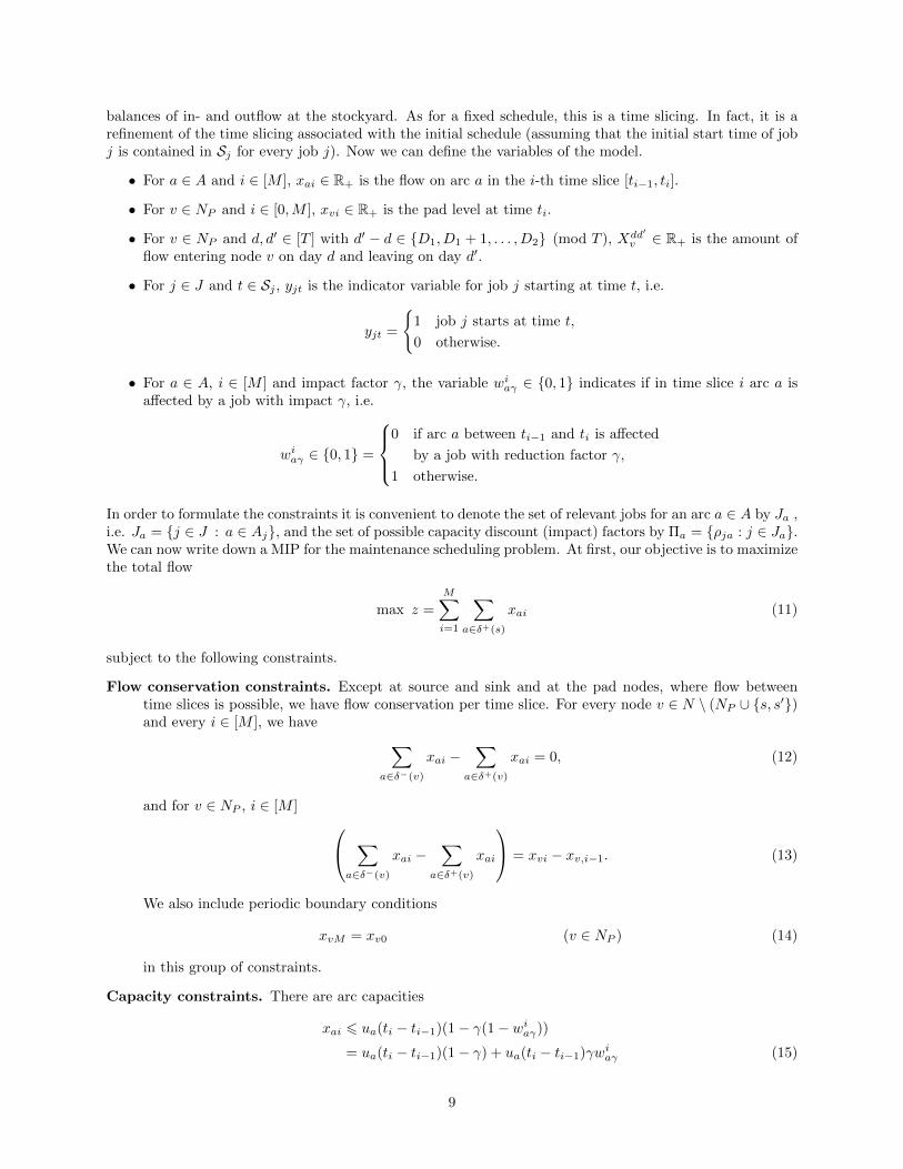
balances of in- and outflow at the stockyard. As for a fixed schedule, this is a time slicing. In fact, it is arefinement of the time slicing associated with the initial schedule (assuming that the initial start time of jobj is contained in Sj for every job j). Now we can define the variables of the model.

• For a ∈ A and i ∈ [M ], xai ∈ R+ is the flow on arc a in the i-th time slice [ti−1, ti].

• For v ∈ NP and i ∈ [0,M ], xvi ∈ R+ is the pad level at time ti.

• For v ∈ NP and d, d′ ∈ [T ] with d′ − d ∈ {D1, D1 + 1, . . . , D2} (mod T ), Xdd′

v ∈ R+ is the amount offlow entering node v on day d and leaving on day d′.

• For j ∈ J and t ∈ Sj , yjt is the indicator variable for job j starting at time t, i.e.

yjt =

{1 job j starts at time t,

0 otherwise.

• For a ∈ A, i ∈ [M ] and impact factor γ, the variable wiaγ ∈ {0, 1} indicates if in time slice i arc a isaffected by a job with impact γ, i.e.

wiaγ ∈ {0, 1} =

0 if arc a between ti−1 and ti is affected

by a job with reduction factor γ,

1 otherwise.

In order to formulate the constraints it is convenient to denote the set of relevant jobs for an arc a ∈ A by Ja ,i.e. Ja = {j ∈ J : a ∈ Aj}, and the set of possible capacity discount (impact) factors by Πa = {ρja : j ∈ Ja}.We can now write down a MIP for the maintenance scheduling problem. At first, our objective is to maximizethe total flow

max z =

M∑i=1

∑a∈δ+(s)

xai (11)

subject to the following constraints.

Flow conservation constraints. Except at source and sink and at the pad nodes, where flow betweentime slices is possible, we have flow conservation per time slice. For every node v ∈ N \ (NP ∪ {s, s′})and every i ∈ [M ], we have ∑

a∈δ−(v)

xai −∑

a∈δ+(v)

xai = 0, (12)

and for v ∈ NP , i ∈ [M ] ∑a∈δ−(v)

xai −∑

a∈δ+(v)

xai

= xvi − xv,i−1. (13)

We also include periodic boundary conditions

xvM = xv0 (v ∈ NP ) (14)

in this group of constraints.

Capacity constraints. There are arc capacities

xai 6 ua(ti − ti−1)(1− γ(1− wiaγ))

= ua(ti − ti−1)(1− γ) + ua(ti − ti−1)γwiaγ (15)

9

for all a ∈ A, i ∈ [M ] and impact factors γ ∈ Πa. Note that this constraint and the use of thew variables exposes the fixed charge network flow structure in the problem. The job start indicatorvariables are linked to the impact indicators via constraints

wiaγ 6 1−∑

t∈Sj : ti−pj6t6ti−1

yjt (16)

for all arcs a ∈ A, all impact factors γ ∈ Πa, all time slice indices i ∈ [M ] and all jobs j ∈ J withρja = γ. In addition, we have node capacities

ulowerv 6 xvi 6 uupperv (17)

for all v ∈ NP and i ∈ [M ]. Note that these are the only lower bounds on flow in the model, so a flowof zero on all arcs, and a flow which is between these bounds and identical for all variables linking astorage node across time slices, provides a feasible solution.

Scheduling constraints. Every job has to be scheduled exactly once, and the processing periods of incom-patible jobs must not overlap.∑

t∈Sj

yjt = 1 (j ∈ J) , (18)

∑j∈C

∑t∈Sj

t<ti6t+pj

yjt 6 1 (i ∈ [M ], C conflict clique), (19)

Dwell time constraints. The values of the flow variables xai determine the total daily in- and outflowsat the pad nodes. Now the inflow of day d has to leave between day d + D1 and day d + D2. This isenforced by the nonnegativity of the variables Xdd′

v and the constraints

d+D2∑d′=d+D1

Xdd′

v =∑

i : dtie=d

∑a∈δ−(v)

xai, (20)

d−D1∑d′=d−D2

Xd′dv =

∑i : dtie=d

∑a∈δ+(v)

xai (21)

for v ∈ NP and d ∈ {1, 2, . . . , T}.

Variable domains. The flow variables are nonnegative reals and the job start indicators are binary.

xai, xvi, Xdd′

v > 0 (a ∈ A, v ∈ NP , i ∈ [M ],

d, d′ ∈ [T ]), (22)

yjt ∈ {0, 1} (j ∈ J, t ∈ Sj), (23)

wiaγ ∈ {0, 1} (a ∈ A, i ∈ [M ], γ ∈ Πa). (24)

In a second phase we change the objective function to maximize the number of jobs starting at their initiallyscheduled start time S0

j :

max∑j∈J

yjS0j, (25)

and we add a lower bound for the total throughput, i.e. a constraint of the form

M∑i=1

∑a∈δ+(s)

xai > B, (26)

where the bound B is a function of the best objective value obtained in the first phase. For our computationalexperiments we just multiplied the maximal throughput by 0.999.

10

5 Solution strategies

In Section 4 we formulated a large scale MIP for the maintenance scheduling of the HVCC. In this sectionwe present some strategies for coping with this large problem. We focus on Phase 1 of the lexicographicoptimization, i.e. on the maximization of the total throughput, as this is the primary objective in practice.For the annual planning more than 2,000 jobs have to be scheduled. After some preprocessing taking intoaccount the rules described in Section 3.2 (fixed jobs, washdowns, etc.) there are still about 1,000 jobscontributing binary variables yjt. In practice, jobs are scheduled by the half-hour or on even finer timescales. If this is accurately modelled, allowing every half-hour in the time window as a potential starttime, a job without additional daylight or weekday constraints has about 14 · 48 = 672 potential start times,corresponding to binary variables. In Subsection 5.1 we describe a heuristic method to choose a representativesubset of the start times. Even with these reduced candidate start time sets initial computational test revealthat the problem for the complete annual time horizon cannot be solved by simple application of a commercialMIP solver (in our case CPLEX 12.3). On the other hand, we obtain promising results if the problem isrestricted to a shorter time horizon. This motivates a rolling horizon approach to the full problem as isdescribed in Subsection 5.2.

5.1 Reducing the number of potential start times

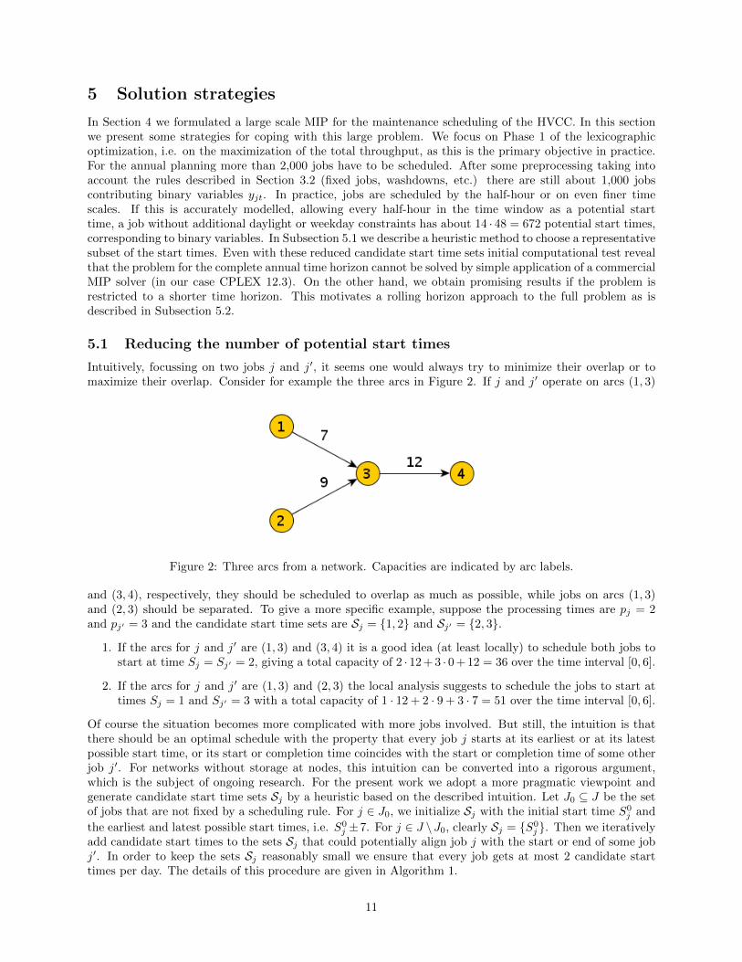
Intuitively, focussing on two jobs j and j′, it seems one would always try to minimize their overlap or tomaximize their overlap. Consider for example the three arcs in Figure 2. If j and j′ operate on arcs (1, 3)

Figure 2: Three arcs from a network. Capacities are indicated by arc labels.

and (3, 4), respectively, they should be scheduled to overlap as much as possible, while jobs on arcs (1, 3)and (2, 3) should be separated. To give a more specific example, suppose the processing times are pj = 2and pj′ = 3 and the candidate start time sets are Sj = {1, 2} and Sj′ = {2, 3}.

1. If the arcs for j and j′ are (1, 3) and (3, 4) it is a good idea (at least locally) to schedule both jobs tostart at time Sj = Sj′ = 2, giving a total capacity of 2 · 12 + 3 · 0 + 12 = 36 over the time interval [0, 6].

2. If the arcs for j and j′ are (1, 3) and (2, 3) the local analysis suggests to schedule the jobs to start attimes Sj = 1 and Sj′ = 3 with a total capacity of 1 · 12 + 2 · 9 + 3 · 7 = 51 over the time interval [0, 6].

Of course the situation becomes more complicated with more jobs involved. But still, the intuition is thatthere should be an optimal schedule with the property that every job j starts at its earliest or at its latestpossible start time, or its start or completion time coincides with the start or completion time of some otherjob j′. For networks without storage at nodes, this intuition can be converted into a rigorous argument,which is the subject of ongoing research. For the present work we adopt a more pragmatic viewpoint andgenerate candidate start time sets Sj by a heuristic based on the described intuition. Let J0 ⊆ J be the setof jobs that are not fixed by a scheduling rule. For j ∈ J0, we initialize Sj with the initial start time S0

j and

the earliest and latest possible start times, i.e. S0j ±7. For j ∈ J \J0, clearly Sj = {S0

j }. Then we iterativelyadd candidate start times to the sets Sj that could potentially align job j with the start or end of some jobj′. In order to keep the sets Sj reasonably small we ensure that every job gets at most 2 candidate starttimes per day. The details of this procedure are given in Algorithm 1.

11

Algorithm 1 Generating start time sets.

for j ∈ J0 do Sj ←{S0j , S

0j − 7, S0

j + 7}

S ←⋃j∈J Sj × {j}

while not STOP dofor j ∈ J0 do

for (t, j′) ∈ S with j′ 6= j dofor t′ ∈ {t, t+ pj′ , t− pj , t+ pj′ − pj} do

if t′ is a feasible start time for job j and∣∣Sj ∩ [bt′c, bt′ + 1c]∣∣ < 2 then

Add t′ to Sj and (t′, j) to Sif none of the sets Sj changed then STOP

5.2 A rolling horizon approach

Computational tests revealed that even after the reduction of the number of binary variables the completeannual problem is very hard. As the performance on restrictions of the problem to shorter time horizonsis better, the iterative solution of smaller subproblems is a natural approach to solving the problem, whichis also supported by the intuition that rescheduling of a job should have mainly local effects: the system’sperformance in September should be largely independent of rescheduling of jobs in March. This suggests thefollowing approach. Fix the binary start indicator variables for all jobs outside a time window [t, t′] and fixall flow variables outside a slightly larger time window [t − δ, t + δ], solve the resulting MIP, shift the timewindows by some value σ,and iterate. The whole procedure is described more precisely in Algorithm 2.

Algorithm 2 The rolling horizon algorithm.

Parameters: w – inner time window widthδ – margin between inner and outer time windowσ – time window shift

Initialize the MIP (11)–(24)for j ∈ J do

for t ∈ Sj doif t = S0

j then yjt ← 1 else yjt ← 0Generate an initial solution from the current values of the variables yjtwhile not STOP

t← 0; t′ ← wwhile t′ < T do

fix all binary variables for jobs j outside [t, t′]fix all continuous variables for time slices outside [t− δ, t′ + δ]solve the problemupdate the start times of jobs j that are not fixedunfix all fixed variablest← t+ σ; t′ ← t′ + σ

6 Computational Results

In this section we present computational results for two real world data sets. We use the raw schedules forthe years 2010 and 2011 as inputs. The capacities for the load point arcs are determined from the annualcapacity forecast numbers for these years. They specify for every load point on a quarterly level the expected

12

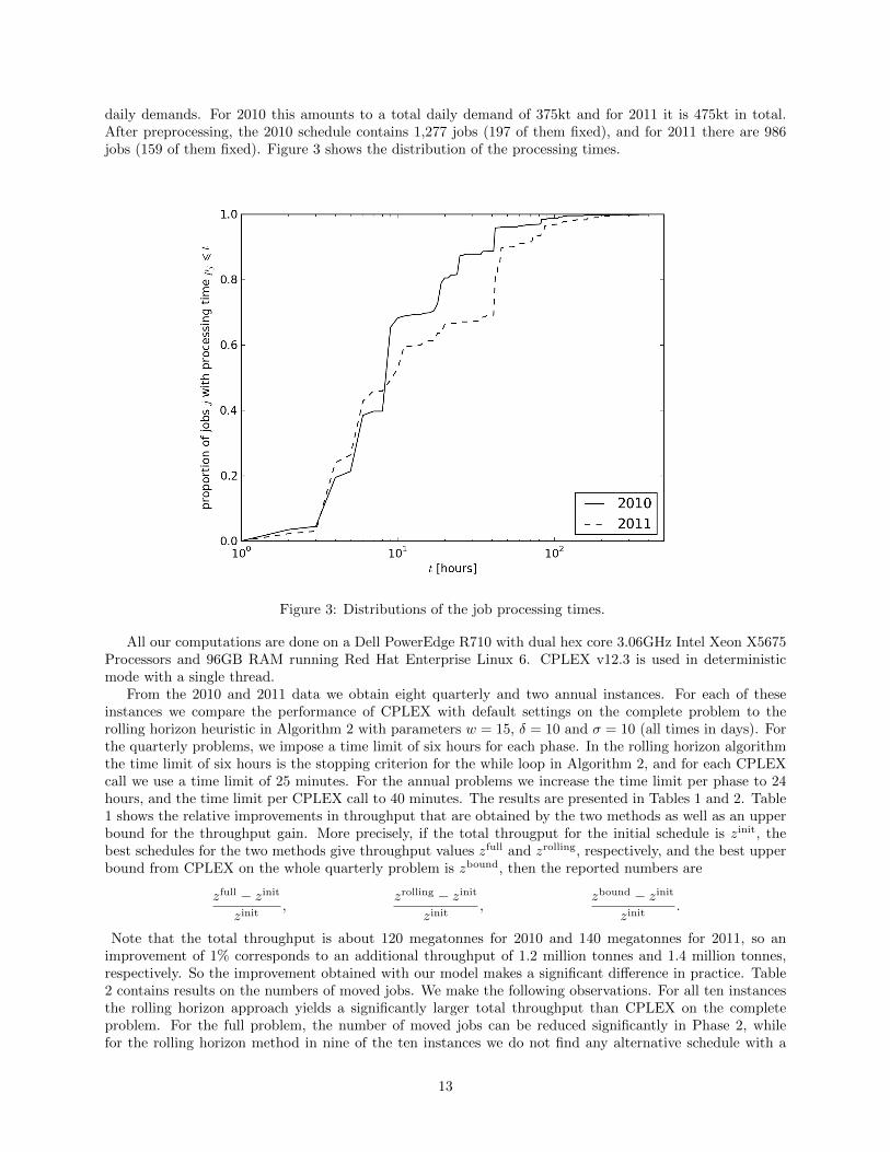
daily demands. For 2010 this amounts to a total daily demand of 375kt and for 2011 it is 475kt in total.After preprocessing, the 2010 schedule contains 1,277 jobs (197 of them fixed), and for 2011 there are 986jobs (159 of them fixed). Figure 3 shows the distribution of the processing times.

Figure 3: Distributions of the job processing times.

All our computations are done on a Dell PowerEdge R710 with dual hex core 3.06GHz Intel Xeon X5675Processors and 96GB RAM running Red Hat Enterprise Linux 6. CPLEX v12.3 is used in deterministicmode with a single thread.

From the 2010 and 2011 data we obtain eight quarterly and two annual instances. For each of theseinstances we compare the performance of CPLEX with default settings on the complete problem to therolling horizon heuristic in Algorithm 2 with parameters w = 15, δ = 10 and σ = 10 (all times in days). Forthe quarterly problems, we impose a time limit of six hours for each phase. In the rolling horizon algorithmthe time limit of six hours is the stopping criterion for the while loop in Algorithm 2, and for each CPLEXcall we use a time limit of 25 minutes. For the annual problems we increase the time limit per phase to 24hours, and the time limit per CPLEX call to 40 minutes. The results are presented in Tables 1 and 2. Table1 shows the relative improvements in throughput that are obtained by the two methods as well as an upperbound for the throughput gain. More precisely, if the total througput for the initial schedule is zinit, thebest schedules for the two methods give throughput values zfull and zrolling, respectively, and the best upperbound from CPLEX on the whole quarterly problem is zbound, then the reported numbers are

zfull − zinit

zinit,

zrolling − zinit

zinit,

zbound − zinit

zinit.

Note that the total throughput is about 120 megatonnes for 2010 and 140 megatonnes for 2011, so animprovement of 1% corresponds to an additional throughput of 1.2 million tonnes and 1.4 million tonnes,respectively. So the improvement obtained with our model makes a significant difference in practice. Table2 contains results on the numbers of moved jobs. We make the following observations. For all ten instancesthe rolling horizon approach yields a significantly larger total throughput than CPLEX on the completeproblem. For the full problem, the number of moved jobs can be reduced significantly in Phase 2, whilefor the rolling horizon method in nine of the ten instances we do not find any alternative schedule with a

13

Full problem Rolling horizon Upper bound

2010 Q1 2.21% 3.01% 4.14%

2010 Q2 1.90% 2.77% 3.28%

2010 Q3 1.70% 2.73% 3.10%

2010 Q4 1.47% 1.82% 2.27%

2010 full 1.61% 2.61% 3.40%

2011 Q1 2.24% 2.53% 2.60%

2011 Q2 1.58% 2.73% 2.96%

2011 Q3 2.39% 3.92% 4.27%

2011 Q4 1.49% 2.13% 2.90%

2011 full 0.00% 1.77% 2.76%

Table 1: Throughput improvements in Phase 1. All numbers are relative improvements compared to theinitial schedule that is used as a start solution. The last column contains upper bounds for the throughputgains.

smaller number of moved jobs that yields at least 99.9% of the throughput achieved in Phase 1. In Phase2 the difference between “full problem” and “rolling horizon” is that the “full problem” has a weaker lowerbound on the throughput from the result of Phase 1. A comparison of the lower bound columns “LB” inTable 2 indicates that there might be a tradeoff between throughput and the number of moved jobs whichshould be studied in more detail in future work.

14

Full problem Rolling horizon

Total P1 P2 LB P1 P2 LB

2010 Q1 342 284 20 14 289 39 26

2010 Q2 384 324 29 17 319 319 41

2010 Q3 293 248 60 16 242 242 40

2010 Q4 266 215 43 15 200 200 26

2010 full 1,277 1,049 1,049 46 1,040 1,040 108

2011 Q1 247 189 18 12 184 184 16

2011 Q2 257 198 11 10 207 207 32

2011 Q3 268 219 16 13 218 218 45

2011 Q4 222 175 17 11 257 257 23

2011 full 986 0 0 0 704 704 40

Table 2: Numbers of moved jobs. We report the total number of jobs (column “Total”), the numbers ofmoved jobs for the final schedule after Phase 1 and Phase 2 (columns “P1” and “P2”) and the lower boundfor the number of moved jobs to achieve the throughput that is enforced in Phase 2 (column “LB”).

7 Concluding remarks

In this paper we present a MIP model for the maintenance scheduling at the HVCC, where the primaryobjective is to maximize the throughput, and the secondary objective is to minimize deviations from a giveninitial schedule. The resulting large scale problems cannot be solved directly, so efficient solution strategiesare needed. We propose an iterative approach based on solving subproblems obtained by fixing most ofthe binary variables. Our computational tests show that this rolling horizon approach outperforms plainCPLEX in terms of the obtained total throughput. Also the experimental results indicate a tradeoff betweenthroughput and the number of moved jobs.

Clearly, more work is necessary in order to improve the performance of the model. Our experimentsindicate that the initial LP bounds are rather weak, so adding appropriate cutting planes is a promisingapproach. Another option for reducing the complexity of the problem is to put an explicit bound on thenumber of moved jobs. This seems to be a reasonable direction, especially as one outcome of discussionswith the maintenance planners was that the option to add more specific constraints on the set of allowedjob movements is a desirable feature. Another step towards a tool that is applicable in practice is thedevelopment of a true bi-objective framework to find (or at least approximate) the set of efficient solutionsfor the objectives “total throughput” and “number of schedule modifications”.

Acknowledgement We like to acknowledge the valuable contributions of Jonathon Vandervoort, RobOyston, Tracey Giles, and the Annual Capacity Alignment Team from the Hunter Valley Coal Chain Co-ordinator (HVCCC) P/L. Without their patience, support, and feedback, this research could not haveoccurred. We also thank the HVCCC and the Australian Research Council for their joint funding under theARC Linkage Grant no. LP0990739.

References

[1] C. Barnhart, N.L. Boland, L.W. Clarke, E.L. Johnson, G.L. Nemhauser and R.G. Shenoi. “Flightstring models for aircraft fleeting and routing”. In: Transportation Science 32.3 (1998), pp. 208–220.doi: 10.1287/trsc.32.3.208.

[2] N. Boland, T. Kalinowski, R. Kapoor and S. Kaur. “Scheduling unit processing time arc shutdownjobs to maximize network flow over time: complexity results”. submitted. 2013.

15

[3] N. Boland, T. Kalinowski, H. Waterer and L. Zheng. “Scheduling arc maintenance jobs in a networkto maximize total flow over time”. In: Discr. Appl. Math. (2012). in press. doi: 10.1016/j.dam.2012.05.027.

[4] N. Boland and M. Savelsbergh. “Optimizing the Hunter Valley coal chain”. In: Supply Chain Disrup-tions: Theory and Practice of Managing Risk. Ed. by H. Gurnani, A. Mehrotra and S. Ray. Springer-Verlag London Ltd., 2011, pp. 275–302.

[5] G. Budai and R. Dekker. “An overview of techniques used in planning railway infrastucture mainten-ance”. In: Proceedings of IFRIMmmm (maintenance modelling and management) Conference. Ed. byW. Geraerds and D. Sherwin. 2002, pp. 1–8.

[6] G. Budai, R. Dekker and R.P. Nicolai. “Maintenance and production: a review of planning models”. In:Complex Systems Maintenance Handbook, Part D. Ed. by K.A.H. Kobbacy and D.N.P. Murthy. Seriesin Reliability Engineering. Springer, 2008. Chap. 13, pp. 321–344. doi: 10.1007/978-1-84800-011-7.

[7] G. Budai, D. Huisman and R. Dekker. “Scheduling preventive railway maintenance activities”. In:Journal of the Operational Research Society 53 (2006), pp. 1035–1044. doi: 10.1057/palgrave.jors.2602085.

[8] D. Frost and R. Dechter. “Optimizing with Constraints: A Case Study in Scheduling Maintenance ofElectric Power Units”. In: Proc. 5th International Symposium on Artificial Intelligence and Mathem-atics. 1998, pp. 1–20.

[9] D. Frost and R. Dechter. “Optimizing with constraints: a case study in scheduling maintenance ofelectric power units”. In: Proc. 5th Int. Conf. on Principles and Practice of Constraint Programming– CP 1998. Ed. by M. Maher and J.-F. Puget. Vol. 1520. LNCS. Springer, 1998, p. 469. doi: 10.1007/3-540-49481-2.

[10] A. Haghani and Y. Shafahi. “Bus maintenance systems and maintenance scheduling: model formula-tions and solutions”. In: Transportation Research Part A: Policy and Practice 36.5 (2002), pp. 453–482.doi: 10.1016/S0965-8564(01)00014-3.

[11] G. Keysan, G.L. Nemhauser and M.W.P. Savelsbergh. “Tactical and operational planning of sched-uled maintenance for per-seat, on-demand air transportation”. In: Transportation Science 44.3 (2010),pp. 291–306. doi: 10.1287/trsc.1090.0311.

[12] R.P. Nicolai and R. Dekker. “Optimal maintenance of multi-component systems: a review”. In: Com-plex Systems Maintenance Handbook, Part D. Ed. by K.A.H. Kobbacy and D.N.P. Murthy. Series inReliability Engineering. Springer, 2008. Chap. 11, pp. 263–286.

[13] A. Sharma, G.S. Yadava and S.G. Deshmukh. “A literature review and future perspectives on main-tenance optimization”. In: Journal of Quality in Maintenance Engineering 17.1 (2011), pp. 5–25. doi:10.1108/13552511111116222.

16