Mixed-Integer Model Predictive Control of Variable-Speed Heat

Pumps

Zachary Lee, Kartikay Gupta, Kevin J. Kircher, K. Max Zhang∗

Sibley School of Mechanical and Aerospace Engineering, Cornell University, Ithaca, New York 14853,United States

Abstract

Heating and cooling buildings cause a large and growing portion of the world’s carbonemissions. These emissions could be reduced by replacing inefficient or fossil-fueled equip-ment with efficient electric heat pumps. Recent research has shown that variable-speedheat pumps (VSHPs) could also provide a variety of power system services, such as price-or carbon-based load shifting, peak demand reduction, emergency demand response, andfrequency regulation. By providing some or all of these services, VSHPs could facilitatethe integration of wind and solar power into the grid, accelerating decarbonization of othereconomic sectors. However, the provision of power system services poses new and challeng-ing VSHP control problems. Model predictive control (MPC) is a promising approach tothese problems. MPC combines weather and load predictions, online optimization, and amathematical model of a VSHP’s performance under varying ambient conditions. With fewexceptions, existing VSHP models neglect two important features that arise in practice: (1)dependence of efficiency and capacity on compressor speed and indoor and outdoor tem-peratures, and (2) inability of VSHPs to operate at low compressor speeds. In this paper,we develop a new VSHP control model that considers both features. The model expressesthe VSHP’s power consumption and heat production as affine functions of the driving tem-peratures and compressor speed. The model also includes a binary variable that constrainsthe VSHP to be either turned off, or operating within a range of acceptable compressorspeeds using mixed-integer programming (MIP). This VSHP model and optimization strat-egy is combined with neural network based heat load prediction in MPC simulations. Thesesimulations suggest that this approach could reduce energy costs by 9 to 22% and carbonemissions by up to 22%, relative to MPC with existing VSHP models.

Keywords: Energy systems; built environment; thermal energy storage; electrification ofthe heating sector

Highlights

• Mixed-integer programming (MIP) is used for variable speed heat pump (VSHP) con-trol.

∗Corresponding authorEmail address: kz33@cornell.edu (K. Max Zhang)

Preprint submitted to Elsevier April 30, 2019

• MIP allows the use of a more complete VSHP model than the current state of the art.

• The improved model reflects partial-load and temperature-dependent VSHP efficiency.5

• MIP reduces operating costs and energy use compared to the current state of the art.

1. Introduction

With rapid growth in population and the floor area of conditioned buildings, globalheating and cooling demand are projected to nearly double by 2050, which have enormous10

economic and environmental consequences [1, 2]. In the United States, for example, heatingand cooling residences cost about $88 billion in 2015 [3]. Heating and cooling costs areparticularly burdensome for people living near the poverty line, often comprising 7–15% oftheir annual income [4, 5]. Space cooling directly contributes to critical peak load during highenergy demand days, when the marginal electricity generation sources are most expensive and15

the atmosphere is most conducive to air pollution formation [6]. Moreover, 60% of UnitedStates homes use natural gas, oil, or propane as their main heating source, contributingto about 10% of the carbon emissions nationwide [3, 7]. Therefore, renewable heating andcooling (RHC), i.e., meeting heating and cooling demand with clean, renewable options atcosts competitive to fossil fuels, is a crucial component in the transition to sustainable energy20

systems.Electric heating and cooling technologies such as air- and ground-source heat pumps

have greatly advanced over the last decade. The leading air-source heat pump models havesignificantly improved their efficiencies at both extremely low (for heating) and high (cooling)ambient temperatures [8]. Powered by renewable electricity generation such as wind and25

solar, heat pumps can potentially become a viable RHC option. RHC viability increases whenthermal energy storage (TES) is added to the heat pump system. TES decouples heat pumpoperation from heating or cooling demand, allowing the heat pump to operate when efficiencyis high and when electricity is clean or inexpensive [9]. Optimal control of heat pumps withand without TES has become a large area of interest as integration of renewable energy30

sources requires more demand flexibility to match the fluctuations in electricity generation[10]. Several studies have already demonstrated the capability of controlling VSHPs withoutenergy storage to provide grid frequency regulation [11, 12]. However, researchers have shownthat coupling heat pumps with TES both increases the instantaneous power flexibility forfrequency regulation [13] and enables demand response and load shifting services on longer35

time scales [14]. These ancillary services are valuable to grid operators and can providenew revenue to VSHP operators [15]. Therefore, we posit that effective heat pump systemcontrol mechanisms that have the ability to provide reliable grid services (e.g., frequencyregulation, demand response, etc.) while maintaining thermal comfort are critical to realizingthe potential of renewable-powered heat pumps as a viable RHC option.40

A major challenge in VSHP control is balancing modeling accuracy with computationalefficiency. VSHP power consumption and heat production are governed by coupled nonlin-ear differential equations, which are unsuitable for control and optimization purposes [16].Thus, simplified but accurate models are needed for real-time control. Constant coefficient

2

of performance (COP) models were adopted in several heat pump control studies [17, 18, 14].45

However, constant COP models neglect the dependency of heat pump performance on com-pressor speed, indoor temperature, and ambient air temperature, thus degrading controllerperformance [19, 20]. In [21], a partial-load and temperature-dependent COP model using athird-order polynomial fit was used to minimize the energy required to cool an office build-ing. However, this model assumes operability over the entire range of partial-load ratios and50

does not consider the reliability constraints associated with running the compressor at lowload ratios.

Recently, Kim et al. [11] demonstrated that in a given compressor speed operatingrange, steady-state VSHP performance behaves linearly with respect to ambient air temper-ature, compressor shaft speed, and indoor air temperature. They formulated a linear model55

to describe the steady-state heat pump thermal output and power consumption in theirdemonstration of frequency regulation applications. However, this linear model is unable tocapture the true heat pump dynamics at low compressor speeds, as it can imply non-zeropower consumption or heat output at zero compressor speed. More discussion of this aspectcan be found in Section S1 of the Supplemental Information. It should be noted that this60

weakness was not an issue for Kim et al., since their study focused on VSHP control in theoperating range and did not consider low compressor speeds [11]. Nevertheless, problems canarise when these linear formulations are used in VSHP control over long time horizons andunder varying boundary conditions. In such applications, VSHP models must be accurateover the entire range of possible compressor speeds and driving temperatures.65

Furthermore, VSHPs are designed to not operate below the minimum manufacturer-ratedcompressor speed. The range of compressor speeds below this value is sometimes referredto as the dead zone. Operating in the dead zone adversely affects the reliability of thecompressor by reducing lubrication thickness and increasing frictional losses [22]. This canreduce the VSHP life and is generally not supported by manufacturers. To avoid this issue,70

if the desired heat load corresponds to a compressor speed in the dead zone, VSHPs will runat the minimum compressor speed for a shorter duration, increasing energy costs by cyclingon and off [23].

The main objective of this paper is to present an effective method for VSHP optimiza-tion and control through mixed-integer programming (MIP). MIP is a method used to solve75

optimization problems when the decision variables are a mixture of continuous and inte-ger variables. While MIP has been used in heat pump studies, the heat pumps are oftenconsidered as single or dual stage thermostatically controlled devices [24, 25]. To our knowl-edge, no studies have applied this method to VSHPs while considering both partial loadand temperature-dependent COPs. In this paper, we use the linear VSHP model developed80

in [11] over the operating range of compressor speeds. This enables the use of online opti-mization, while capturing the dependence of COP on compressor speed, indoor temperature,and outdoor temperature. In addition, we introduce a binary variable into the optimizationprocess to indicate whether the VSHP is turned on. This innovation allows the heat pumpto turn off rather than operate below the minimum rated compressor speed, preventing op-85

eration in the dead zone and solving the issue of unrealistic model results at low compressorspeeds. We demonstrate the effectiveness of the proposed MIP approach by applying modelpredictive control (MPC) to a realistic heat pump control problem. MPC has been widelyemployed in a range of heat pump and TES scenarios and has been shown to be an effective

3

way to optimize heat pump costs [26, 27, 28]. This simulation includes real-world electric-90

ity rates, historical meteorological conditions, a high-fidelity building thermal model, and aneural network based heat load prediction method to provide VSHP control performance fora winter season.

This paper is organized as follows. Section 2 models the heat pump, TES, and buildingthermal envelope. Section 3 formulates the control problem, describes the proposed mixed-95

integer MPC algorithm, and discusses three simpler but more common controllers. Section4 compares the performance of the four controllers. Section 5 concludes the paper.

2. Thermal modeling

We modeled a single corner apartment in a mid-rise apartment building. The unit isequipped with a VSHP in series with TES. The VSHP pumps heat from the outside air into100

the TES, which then serves the building heating demand. This design allows the TES tofunction as a heat battery, giving the VSHP more operational flexibility. While we focusedon heating, our methods can also be used for cooling, as VSHPs are reversible. We modelthe three physical components – the VSHP, TES and building envelope – in the remainderof this section.105

2.1. Variable speed heat pump

To capture the dynamics of a VSHP, we adopted the linear model formulated by Kimet al. [11] Shown in Equation 1, this model gives the steady-state power consumption Ptand heat production Ht at a time step t as affine functions of the compressor speed, indoortemperature, and outdoor air temperature:110

Power Consumption: Pt = α1 + α2ωt + α3Th,t + α4Ta,t

Heat Output: Ht = α5 + α6ωt + α7Th,t + α8Ta,t.(1)

Here ωt (rad/s) is the compressor speed, Th,t (◦C) is the TES temperature, and Ta,t (◦C) isthe ambient temperature. The model coefficients αi can be fit to empirical performance datavia multiple linear regression. Experimental results in [29] show that the efficiency reductionassociated with startup and shutdown of a heat pump is 2% or less for a duty cycle of 15minutes. Therefore, we assume this reduced performance during startup is negligible because115

the MPC updates each hour. The VSHP efficiency, referred to as the COP, is defined as theratio of the heat output to the power consumption:

COP =PtHt

. (2)

For this simulation, we used performance data from Carrier’s Infinity Series VSHP(Model: 25VNA024A) [30] to determine the best-fit model coefficients. Table 1 shows thebest-fit coefficients. Figure 1 shows a subset of the manufacturer data and the resulting120

linear equations for power consumption and heat output at an indoor air temperature of21.1◦C. The R-squared values for power consumption and heat output are given as .996 and.994, respectively. While publicly available data detailing partial load VSHP performance istypically very limited, linear performance in the operating range was already experimentally

4

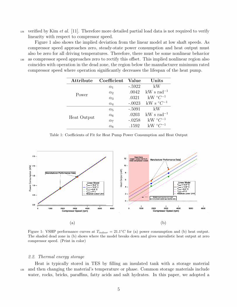
verified by Kim et al. [11]. Therefore more detailed partial load data is not required to verify125

linearity with respect to compressor speed.Figure 1 also shows the implied deviation from the linear model at low shaft speeds. As

compressor speed approaches zero, steady-state power consumption and heat output mustalso be zero for all driving temperatures. Therefore, there must be some nonlinear behavioras compressor speed approaches zero to rectify this offset. This implied nonlinear region also130

coincides with operation in the dead zone, the region below the manufacturer minimum ratedcompressor speed where operation significantly decreases the lifespan of the heat pump.

Attribute Coefficient Value Units

Power

α1 -.5922 kWα2 .0042 kW s rad−1

α3 .0321 kW ◦C−1

α4 -.0023 kW s ◦C−1

Heat Output

α5 -.5091 kWα6 .0203 kW s rad−1

α7 -.0258 kW ◦C−1

α8 .1592 kW ◦C−1

Table 1: Coefficients of Fit for Heat Pump Power Consumption and Heat Output

(a) (b)

Figure 1: VSHP performance curves at Tindoor = 21.1◦C for (a) power consumption and (b) heat output.The shaded dead zone in (b) shows where the model breaks down and gives unrealistic heat output at zerocompressor speed. (Print in color)

2.2. Thermal energy storage

Heat is typically stored in TES by filling an insulated tank with a storage materialand then changing the material’s temperature or phase. Common storage materials include135

water, rocks, bricks, paraffins, fatty acids and salt hydrates. In this paper, we adopted a

5

general model that can represent a variety of temperature- and phase-change thermal storagetechnologies. The basic model is a first-order continuous-time linear system:

E(t) = βE(t) + Q(t)

0 ≤ E(t) ≤ Emax.(3)

Here t (h) denotes time, E (kWh) is the stored heat, and Q (kW) is the net heat flow intostorage. For a given storage technology, the parameter β (1/h) and the storage capacity Emax140

(kWh) can be defined in terms of the storage dimensions and thermophysical properties. Forcontrol purposes, we considered a continuous time span t ∈ [0, K∆t], divided into K discretesteps of duration ∆t (h), indexed by k = 0, . . . , K. Assuming that the net heat flow Q isconstant over each time step, Q(t) = Q(k∆t) for all t ∈ [k∆t, (k + 1)∆t). With E andQ at a time step k denoted by Ek and Qk, respectively, the discrete-time analog of the145

continuous-time storage model (3) is

Ek+1 = aEk + bQk, k = 0, . . . , K − 1

0 ≤ Ek ≤ Emax, k = 1, . . . , K.(4)

The discrete-time parameters are defined in terms of β and ∆t:

a = eβ∆t, b =a− 1

β.

These definitions follow from the solution of the governing differential equation (3).

2.3. Building envelope

To determine space heating load, we simulated a mid-rise corner apartment facing south-150

east in Binghamton, NY, using EnergyPlus [31]. EnergyPlus is an open-source whole-building simulation software package that considers indoor and outdoor air temperatures,solar radiation, and other weather values, as well as internal heat loads and building oc-cupancy. The simulated building is the mid-rise commercial reference building developedin [32], which uses the most common construction materials, energy usage, and occupancy155

schedules. The indoor thermostat setpoint is 21.7 ◦C. The outside weather conditions camefrom three weather files for Binghamton, NY: a Typical Meteorological Year (TMY3) andreal data from the years 2001 and 2014 [31, 33]. The TMY3 file for Binghamton is derivedfrom 24 years of historical weather data and provides a weather profile that represents a typ-ical year [33]. The TMY3 and 2001 weather files provide a range of conditions that we used160

to train our model. We then simulated the controller performance under the 2014 weatherdata.

2.4. State-space system model

By combining the linear model in Equation 1 with the discrete time energy storageformulation in Equation 4, a state space model is developed:165

xk+1 = axk + α6buk + wk. (5)

6

Here the state xk (kWh) is the stored TES energy Ek, the control input uk (rad/s) is thecompressor speed ωk, and the disturbance wk is a function of the outdoor air temperature(◦C) and building heat demand (kW).

Specific disturbances can be defined for different TES types and system configurations.In our simulation, we modeled a stratified water tank, the most common form of residential170

TES. Stratified water tanks can be closely approximated to have two layers: a hot layer andcold layer with time-invariant temperatures Th and Tc, respectively [34]. Depending on theamount of thermal energy stored, the thermocline separating these layers will move up anddown in the tank, where the maximum and minimum energy storage limits correspond tothe minimum and maximum operating height of the thermocline. For a stratified water TES175

in series with a VSHP, the system’s disturbance is defined as

wk = b [α5 + α7Th − Tc/R + (α8 + 1/R)Ta,k −Qd,k] .

Here R (◦C/kW) is the thermal resistance of the thermal storage tank wall and Qd,k (kW)is the space heating demand.

3. Control and prediction

In this section, we formulate the problem of optimally operating the combined heat180

pump and thermal storage system using MPC. MPC is a control method that predictssystem behavior to develop an optimal control schedule for a receding time horizon. MPCis constructed of three main components: (1) a system control model, (2) an optimizationframework, and (3) an accurate prediction model for future system inputs.

3.1. Control policies185

MPC requires a detailed system control model to determine optimal control schedules.Increasing the physical accuracy of the control model should generally increase MPC per-formance. However, increasing complexity can cause models to switch from convex to non-convex. While convex optimization algorithms can quickly provide absolute optimal control,non-convex optimization is generally more computationally expensive and relies on heuristic190

solution methods that can only provide near optimal control. Therefore, the challenge isto design a physically realistic control model that does not significantly hurt optimizationtime and performance. In our study, we analyzed four VSHP control policies, each withdecreasing complexity. The proposed MIP control is used in Policy 1, while Policies 2, 3,and 4 are used as a comparison and represent simpler, more commonly used VSHP con-195

trol models. The minimum compressor speed constraint in Policy 1 is embedded into theoptimization through MIP, which allows the VSHP to turn off when below the minimumcompressor speed. For Policies 2, 3, and 4, this constraint is applied by post-processing thecontrol schedule after the optimization process. If the optimization calls for a compressorspeed below the minimum speed, the speed is set at the minimum and run for a percentage200

of the time step to provide an equivalent amount of heat. The true dynamics of the ther-modynamic system are updated using Equation 1, which was experimentally verified in [11]to be applicable across the range of operating compressor speeds. Table 2 summarizes thedetails of each of the control policies.

7

3.1.1. Policy 1: Mixed-integer MPC205

MIP is used to solve optimization problems when a portion of the decision variables areconstrained to be integer values. Constraining some variables to be integer values causesthe problem to become non-convex, and a global optimal solution becomes more difficult tofind. Common algorithms for solving MIP problems include branch and bound as well asheuristic methods such as tabu search and simulated annealing [35].210

Despite the increased difficulty of finding an optimal solution, MIP allows the use ofa more physically realistic control model that considers COP dependence on compressorspeed, outdoor air temperature, and TES temperature. It solves the issue of unrealisticmodel results at low compressor speeds by using a binary variable in the optimization toallow the heat pump to turn off when below the minimum compressor speed. When the215

heat pump is on, it operates between the minimum and maximum compressor speeds andcalculates power consumption and heat output using Equation 1. When the heat pump isoff, power consumption and heat output are zero, satisfying the boundary condition at zerocompressor speed. This model is shown in Equation 6 with ωmin and ωmax as the minimumand maximum rated compressor speeds, respectively,220

Pt,MIP , Ht,MIP =

{Pt, Ht ωmin ≤ ω ≤ ωmax

0 0 ≤ ω < ωmin

. (6)

3.1.2. Policy 2: MPC with linear COP

Policy 2 does not consider COP dependence on compressor speed and only considersCOP as a linear function of outdoor air temperature and TES temperature. This modelis therefore convex and can provide an absolute optimal solution. To determine the linearfunction for COP, Equation 1 was evaluated at the maximum compressor speed over the225

operating range of winter temperatures to create a linear regression model with the resultinglinear equation:

COP = .0446Tamb + 2.77. (7)

3.1.3. Policy 3: MPC with Constant COP

Policy 3 assumes a constant COP model regardless and neglects COP dependence oncompressor speed and driving temperatures. While seasonal average VSHP COPs are often230

given by the manufacturer in the form of the heating seasonal performance factor (HSPF), itis important that the constant COP used in the optimization is sized much lower to accountfor times of low ambient air temperature. Since VSHP COP and capacity are small whenambient temperatures are low, using an inflated COP can cause the control scheme to beunable to meet the required heat load at those times. For this reason, the constant COP235

for Policy 2 was conservatively set at 2.0, which corresponds to the COP at the low rangeof operating temperatures.

3.1.4. Policy 4: No TES or optimization

Policy 4 uses only a VSHP without optimization or thermal energy storage to providea baseline comparison. In this policy, the VSHP exactly provides the heat load from the240

residence, which is the most common way for VSHPs to operate. Any control optimization

8

worth implementing should first be able to outperform Policy 4. We assumed that the indoorair temperature remains constant at the same setpoint used in the EnergyPlus simulationat 21.7 ◦C.

PolicyControlPolicy

ConvexityThermal Energy

Storage1 Mixed-integer Non-convex Yes2 Linear COP Convex Yes3 Constant COP Convex Yes4 None N/A No

Table 2: Summary of Optimization Policy Details

3.2. Optimization framework245

The optimization framework must ensure that the VSHP electricity cost is minimizedwhile maintaining thermal comfort of the occupants. The discretized VSHP electricity costge,k at a time step k can be written as:

ge,k(uk, wk) = ψe,k∆tPkyk. (8)

Here ψe,k ($/kWh) is the utility’s hourly residential time-of-use rate given deterministically.In this simulation, we use New York State Electric and Gas Corporation’s (NYSEG) time-250

of-use electricity supply rate [36]. We only considered the electricity supply rate since taxesand delivery charges contributing to the total electricity cost are time invariant and varygeographically. The time step is given by ∆t (h). The heat pump power consumption ata time step k is given by Pk (W) and is calculated using Equation 1. The binary variableused to implement MIP is given by yk and can have values of zero or one. When yk is zero,255

the heat pump is turned off and the electricity cost is zero. When yk is one, the compressormust operate between the minimum and maximum speeds. For Policies 2, 3, and 4, yk wasset constant at one and the minimum compressor speed was set at zero, since the controlpost-processing described in Section 3.1 satisfies the compressor speed constraint.

In addition, the TES should not be over or undercharged, as this could be unsafe, decrease260

efficiency, and decrease occupant comfort. Therefore, an upper limit and lower limit tothe amount of energy stored in the thermal storage was imposed, given by EU and EL,respectively. Moreover, having a certain amount of energy storage stored at all times ispreferable, as prediction and model uncertainties can cause the scheduled heat supply to beinsufficient to meet heat load. Therefore, a tunable penalty parameter ψL was included to265

penalize when thermal energy is below a desired percentage of TES capacity γ,

gd,k(xk) = ψL(γEU − xk)+, (9)

Together, these constraints and cost functions construct the optimization framework andare shown in Equation 10, where N is the control horizon. To minimize this function we

9

used the Gurobi solver [37] in the convex optimization software CVX [38], which are capableof efficiently solving mixed-integer linear programs.270

minimizeu

N∑k=1

(ge,k + gd,k),

subject to EL ≤ xk+1 ≤ EU , k = 1, . . . , N,

ykωmin ≤ uk ≤ ykωmax k = 1, . . . , N.

(10)

3.3. Data-Driven Heat Load PredictionsTo efficiently plan the future control scheme, MPC requires predictions of future heat

load requirements and outdoor air temperature. We assumed a perfect temperature forecastsince publicly available day-ahead temperature forecasts are often within 1◦C of the actualtemperature values [39]. To predict heat load, we used a Long Short Term Memory (LSTM)275

recurrent neural network. LSTM networks excel in learning patterns in sequence data byencoding important information into memory cells that can be used many time steps in thefuture. This memory cell mitigates the problem of exploding and vanishing gradients whenusing a large number of previous time steps as an input to the network.

The main neural network architecture consists of an LSTM layer followed by three fully280

connected layers and an output layer. The previous 22 hours are used as an input into theLSTM layer, which has an auxiliary output layer to facilitate the LSTM layer training. Thisauxilliary output ensures that the LSTM layer can learn the patterns of the time-series datawithout them being distorted by the fully connected layers. The 24-hour ahead temperaturepredictions are then concatenated with the LSTM output as input into the fully connected285

layers. The main output layer then outputs the 24-hour ahead heat load predictions. Thenetwork is trained using the mean squared error loss function. Figure 2 shows the full neuralnetwork architecture. Optimal hyperparameters were determined through a randomized gridsearch and are shown in Table 3.

Figure 2: Neural network architecture

Layer Neurons ActivationLSTM 399 tanh

Fully Connected 1 139 sigmoidFully Connected 2 84 sigmoidFully Connected 3 323 relu

Hyperparameters ValueOptimizer Adam

Learning Rate .003

Input ValuePrevious Time Steps 22

Table 3: Neural network hyperparametersobtained through randomized grid search

Hourly training data came from the EnergyPlus simulation for an average mid-rise corner290

apartment in Binghamton, NY, over the the course of the TMY3 and 2001 winter seasons

10

(December 1 to February 28). The model was trained on 3,592 hourly samples with 634hourly samples used for model validation and hyperparameter tuning. The model was thenused to predict the hourly heat load for the same simulated building using real weather datafrom the specific year 2014 in a continuous learning model. Each week, the previous week’s295

hourly samples were added to the training dataset, and the neural network was retrained onthe slightly larger dataset. This most closely models a real world scenario where predictionmodels can continuously improve from the constant stream of new data. Figure 3 shows theFebruary 2014 heat load predictions for 1 hour ahead, 12 hours ahead, and 24 hours ahead.These figures show that apart from extremely high or low values, the prediction error is low300

and therefore does not compound to significantly effect heat load predictions many hours inthe future.

4. Results and discussion

Simulations provided optimal control schedules for each of the control policies for the win-ter of 2014. The simulations were run continuously from December 1st, 2013 until February305

28th, 2014 with an MPC horizon of 24 hours updating each hour. Figure 4 shows a subsetof the optimal control schedules and the corresponding temperature and electricity price fora five day range in January. Table 4 gives the total energy consumption and electricity costfor the entire winter. It is important to note that this table shows the electricity supply cost,which is only about 30% to 50% of the total electricity cost depending on residence location310

and taxes.

4.1. Control policy performance

Policy 1 (MIP) provided both the lowest energy consumption and the lowest electricitycost because it can optimize using all relevant knowledge: dynamic electricity price, com-pressor frequency, and ambient air temperature. Figure 4b shows Policy 1’s preference for315

running less often but with higher power consumption, since Equation 1 results in a higherCOP at higher compressor speeds. Policy 2 behaved similarly to Policy 1, concentratingpower consumption toward high efficiency, low cost hours. However, the linear COP modelof Policy 2 does not capture the COP dependence on compressor speed and therefore oper-ated at low compressor speeds for some hours, reducing the efficiency. Policy 3 concentrated320

operation toward times of low electricity cost during the night. However, this is often the

Policy ModelTotal Energy

Consumption (kWh)Electricity Supply

Cost ($)1 MIP 846 32.282 Linear COP 921 35.433 Constant COP 1086 41.66

4No TES or

optimization1086 48.77

Table 4: Total simulation results for winter of 2014: Using MIP in Policy 1 significantly reduces electricityusage compared to simpler, more commonly used VSHP control policies.

11

(a) 1 Hour Ahead Heat Load Predictions

(b) 12 Hours Ahead Heat Load Predictions

(c) 24 Hours Ahead Heat Load Predictions

Figure 3: Heat load predictions for (a) 1 hour ahead and (b) 12 hours ahead, and (c) 24 hours ahead. Apartfrom extreme values, the prediction error is low and does not accumulate for predictions many hours ahead.

least efficient time to operate due to low outdoor air temperatures, resulting in no decreasein energy consumption compared to the baseline Policy 4. The non-convexity of Policy 1also incurred only a marginal increase in average computational time of 19% when comparedto the convex models in Policies 2 and 3.325

Without any optimization or TES, Policy 4 performed significantly worse than the mod-els using TES and MPC, showing that MPC can have a large positive impact on reducingoperating costs. However, this reduction in operating costs is limited by the accuracy of theprediction model. For example, a perfect prediction model of future heat load and outdoortemperature can further reduce the operating cost by up to 6% when compared to the pro-330

12

Figure 4: A subset of the control plots for a five day period in January for each control policy. Policy 1(MIP) runs less frequently at a higher average speed compared to each of the comparison studies, giving ahigher average COP and less total energy consumption and cost.

13

posed prediction model. Therefore, an accurate prediction model is required to capture thefull potential benefit of MPC. While the proposed mixed-integer MPC significantly reducesoperating costs, the total economic viability of implementing TES and MPC into a homeheated by a VSHP requires a more detailed economic analysis on capital costs specific to theresidence.335

Finally, reducing energy consumption can have a direct impact on reducing carbon emis-sions. A recent report from the New York Independent System Operator (NYISO) statedthat the marginal energy source in Binghamton and Central New York is almost alwaysnatural gas [40]. In this case, assuming that a decrease in energy consumption correspondsto a proportional reduction in carbon emissions, Policy 1 (MIP) reduces carbon emissions340

by 8.1%, 22.1%, and 22.1% relative to Policies 2, 3, and 4, respectively.

4.2. Infeasibility of the linear model without MIP

Additional simulations were run using the linear program relaxation of the MIP formula-tion of Policy 1. This control policy used the linear model of Equation 1 without the integervariable, allowing the compressor speed to range from zero to the maximum. If the optimal345

compressor speed fell below the minimum, the compressor speed was post-processed in thesame format of Policies 2 through 4. However, this formulation proved to be unrealistic andcaused feasibility errors during the optimization process. This is because the linear modelgives non-zero heat output at zero compressor speed, disallowing the heat pump to turnoff. Under certain boundary conditions, this causes the TES to charge indefinitely, violating350

the TES limit constraints. Therefore, this type of control policy does not provide a validcomparison to Policies 1 through 4.

4.3. Effect of TES on control performance

The potential benefit of TES on MPC performance is highly dependent on the variance ofboth outdoor air temperature and electricity time-of-use rates. All else equal, with a higher355

difference between the maximum and minimum of these values, the optimization can takeadvantage of times of even higher efficiency or lower electricity costs. When compared to thebaseline Policy 4, the addition of cost-based optimization in Policy 3 provided a large decreasein energy cost of 14.6%. However, the addition of the complete efficiency-based optimizationin Policy 1 resulted in a further cost reduction of 22.5% when compared to Policy 3. This360

difference implies that the efficiency-based optimization is more effective than the cost-based optimization for this scenario. Binghamton, NY, with an above average number ofcloudy days, experiences relatively small temperature swings, limiting the potential benefitof efficiency-based optimization. Therefore, simulating the climate in Binghamton serves asa baseline to show that including the complete cost- and efficiency-based optimization of365

Policy 1 should outperform other control policies even more in most other climates.The size of the TES had relatively little effect on the efficiency of the control schemes

as long as the TES has the capacity to provide heat load for the control horizon. Theenergy stored in the TES is optimized to be low to reduce energy loss to the ambient, aswell as to minimize costs across the control horizon. Increasing the control horizon could370

take better advantage of increased TES capacity; however, this comes with a reductionin forecasting accuracy and increased computational time. Other effects that involve the

14

unsteady thermodynamics of the TES could have an effect on the optimization but wereassumed to be negligible due to the relatively long hourly time scale of the optimization.

5. Conclusion375

This paper presents a computationally efficient but realistic variable speed heat pumpcontrol optimization model using MIP that solves the unphysical characteristics of linearVSHP models at low compressor speeds. In addition, it prevents the operation of the heatpump in the compressor dead zone, which reduces the life span of the heat pump. By usingmachine learning methods to predict future heat load and ambient air temperatures, this380

method can provide optimal VSHP control schedules for a given time horizon using MPC.While existing VSHP control models often do not consider all variables affecting VSHP COP,using MIP allows the use of a more complete VSHP model that captures COP based onoutdoor air temperature, indoor temperature, and compressor speed. The proposed methodoutperforms existing VSHP control policies by reducing electricity costs by 9 and 22% and385

reducing carbon emissions by up to 22%. Since VSHPs and TES can provide ancillaryservices to the grid in the form of load shifting or frequency regulation, future work canexplore expanding this control scheme to include grid signals on faster time scales. Overall,this control method can go toward reducing electricity costs for residences with VSHPs andTES, diminishing barriers to more efficient and renewable heating and cooling options.390

15

Acknowledgments

The authors acknowledge the support from the National Science Foundation (NSF) un-der grant 1711546 and the valuable discussions with Prof. H. Ezzat Khalifa at SyracuseUniversity and Prof. Youngjin Kim at Pohang University of Science and Technology, Korea.

Declaration of Interest395

Declarations of interest: none

References

[1] B. Dean, J. Dulac, K. Petrichenko, P. Graham, Towards zero-emission efficient and re-silient buildings: Global Status Report, Global Alliance for Buildings and Construction(GABC), 2016.400

[2] D. Urge-Vorsatz, L. F. Cabeza, S. Serrano, C. Barreneche, K. Petrichenko, Heatingand cooling energy trends and drivers in buildings, Renewable and Sustainable EnergyReviews 41 (2015) 85–98.

[3] US Energy Information Administration, Residential Energy Consumption Survey,https://www.eia.gov/consumption/residential/data/2015/index.php/, 2018.405

[4] A. Drehobl, L. Ross, Lifting the high energy burden in Americas largest cities, AmericanCouncil for an Energy-Efficient Economy (ACEEE), 2016.

[5] NYSERDA Low- to moderate-income market characterization report, New York StateEnergy Research and Development Authority (NYSERDA), 2017.

[6] X. Zhang, K. M. Zhang, Demand response, behind-the-meter generation and air quality,410

Environmental Science & Technology 49 (2015) 1260–1267.

[7] S. Billimoria, M. Henchen, L. Guccione, L. Louis-Prescott, The Economics of Electri-fying Buildings: How Electric Space and Water Heating Supports Decarbonization ofResidential Buildings, Rocky Mountain Institute, 2018.

[8] R. Aldrich, J. Grab, D. Lis, Northeast/Mid-Atlantic Air-Source Heat Pump Market415

Strategies Report 2016 Update, Northeast Energy Efficiency Partnerships, 2017.

[9] S. N. Palacio, K. F. Valentine, M. Wong, K. M. Zhang, Reducing power system costswith thermal energy storage, Applied Energy 129 (2014) 228–237.

[10] P. Sorensen, N. A. Cutululis, A. Vigueras-Rodrıguez, L. E. Jensen, J. Hjerrild, M. H.Donovan, H. Madsen, Power fluctuations from large wind farms, IEEE Transactions on420

Power Systems 22 (2007) 958–965.

[11] Y. J. Kim, L. K. Norford, J. L. Kirtley, Modeling and Analysis of a Variable Speed HeatPump for Frequency Regulation Through Direct Load Control, IEEE Transactions onPower Systems 30 (2015) 397–408.

16

[12] E. Vrettos and G. Andersson, Scheduling and Provision of Secondary Frequency Re-425

serves by Aggregations of Commercial Buildings, IEEE Transactions on SustainableEnergy 7 (2016) 850–864.

[13] C. Finck, R. Li, R. Kramer, W. Zeiler, Quantifying demand flexibility of power-to-heatand thermal energy storage in the control of building heating systems, Applied Energy209 (2018) 409–425.430

[14] B. Alimohammadisagvand, J. Jokisalo, S. Kilpelainen, M. Ali, K. Siren, Cost-optimalthermal energy storage system for a residential building with heat pump heating anddemand response control, Applied Energy 174 (2016) 275–287.

[15] B. Kirby, Ancillary Services: Technical and Commercial Insights, Wartsila North Amer-ica Inc, 2007.435

[16] X.-D. He, Dynamic modeling and multivariable control of vapor compression cycles inair conditioning systems, Ph.D. thesis, Department of Mechanical Engineering, Mas-sachusetts Institute of Technology, 1996.

[17] M. Awadelrahman, Y. Zong, H. Li, C. Agert, Economic Model Predictive Control forHot Water Based Heating Systems in Smart Buildings, Energy and Power Engineering440

9 (2017) 112–119.

[18] R. Halvgaard, N. K. Poulsen, H. Madsen, J. B. Jorgensen, Economic model predictivecontrol for building climate control in a smart grid, 2012 IEEE PES Innovative SmartGrid Technologies (ISGT) (2012) 1–6.

[19] C. Verhelst, F. Logist, J. V. Impe, L. Helsen, Study of the optimal control problem445

formulation for modulating air-to-water heat pumps connected to a residential floorheating system, Energy and Buildings 45 (2012) 43–53.

[20] A. Bloess, W.-P. Schill, A. Zerrahn, Power-to-heat for renewable energy integration: Areview of technologies, modeling approaches, and flexibility potentials, Applied Energy212 (2018) 1611–1626.450

[21] T. Zakula, P. R. Armstrong, L. Norford, Modeling environment for model predictivecontrol of buildings, Energy & Buildings 85 (2014) 549–559.

[22] S. Shao, W. Shi, X. Li, H. Chen, Performance representation of variable-speed com-pressor for inverter air conditioners based on experimental data, International Journalof Refrigeration 27 (2004) 805 – 815.455

[23] N. Saraf, Predictive Control for Residential Capacity Controlled Heat Pumps in a SmartGrid Scenario, Master’s thesis, Delft University of Technology, 2015.

[24] M. C. Bozchalui, S. A. Hashmi, H. Hassen, C. A. Canizares, K. Bhattacharya, Optimaloperation of residential energy hubs in smart grids, IEEE Transactions on Smart Grid3 (2012) 1755–1766.460

17

[25] G. Bianchini, M. Casini, A. Vicino, D. Zarrilli, Demand-response in building heatingsystems: A model predictive control approach, Applied Energy 168 (2016) 159 – 170.

[26] D. Fischer, T. R. Toral, K. B. Lindberg, B. Wille-Haussmann, H. Madani, Investigationof thermal storage operation strategies with heat pumps in German multi-family houses,Energy Procedia 58 (2014) 137–144.465

[27] T. Q. Pean, J. Salom, R. Costa-Castello, Review of control strategies for improvingthe energy flexibility provided by heat pump systems in buildings, Journal of ProcessControl (2018).

[28] Candanedo, Jose and Dehkordi, Vahid R., Simulation of Model-based Predictive Con-trol Applied to a Solar-assisted Cold Climate Heat Pump System, International High470

Performance Buildings Conference (2014).

[29] M. Uhlmann, S. S. Bertsch, Theoretical and experimental investigation of startup andshutdown behavior of residential heat pumps, International Journal of Refrigeration 35(2012) 2138–2149.

[30] Carrier, 25VNA Infinity Variable Speed Heat Pump with Greenspeed Intelligence475

2 to 5 Nominal Tons, https://www.carrier.com/residential/en/us/products/

heat-pumps/25vna0, 2011.

[31] D. B. Crawley, C. O. Pedersen, L. K. Lawrie, F. C. Winkelmann, Energyplus: Energysimulation program, ASHRAE Journal 42 (2000) 49–56.

[32] M. Deru, K. Field, D. Studer, K. Benne, B. Griffith, P. Torcellini, B. Liu, M. Halverson,480

D. Winiarski, M. Rosenberg, et al., U.S. Department of Energy Commercial ReferenceBuilding Models of the National Building Stock, National Renewable Energy Labora-tory, 2011.

[33] S. Wilcox, W. Marion, Users Manual for TMY3 Data Sets (Revised), National Renew-able Energy laboratory, 2008. doi:10.2172/928611.485

[34] J. Waluyo, M. Abd Majid, Temperature profile and thermocline thickness evaluationof a stratified thermal energy storage tank, International Journal of Mechanical andMechatronics Engineering 10 (2010).

[35] A. Richards, J. How, Mixed-integer programming for control, Proceedings of the 2005,American Control Conference. (2005) 2676–2683 vol. 4.490

[36] New York State Electric and Gas Corporation, Electricity service rate, 2018. Serviceclass 12, Rate No. 115-12-00.

[37] Gurobi Optimization, Gurobi Optimizer Version 8.1, http://www.gurobi.com/, 2018.

[38] M. Grant and S. Boyd, CVX: Matlab Software for Disciplined Convex Programming,Version 2.1, Build 1123, http://cvxr.com/cvx/, 2018.495

18

[39] B. Rose, E. Floehr, Analysis of High Temperature Forecast Accuracy of ConsumerWeather Forecasts from 2005-2016, Intellovations, LLC, 2017.

[40] D. B. Patton, P. LeeVanSchaick, J. Chen, R. P. Naga, 2017 State of the Market Reportfor the New York ISO markets, New York Independent System Operator, Inc., 2017.

19