MIXED FINITE ELEMENTS, COMPATIBILITY CONDITIONS AND...
63
D.Boffi F.Brezzi L.Demkowicz R.G.Dur´ an R.S.Falk M.Fortin MIXED FINITE ELEMENTS, COMPATIBILITY CONDITIONS AND APPLICATIONS Lectures given at the C.I.M.E. Summer School held in Cetraro, Italy, June 26-July 1, 2006 Editors: D. Boffi, L. Gastaldi Springer Berlin Heidelberg NewYork Hong Kong London Milan Paris Tokyo
Transcript of MIXED FINITE ELEMENTS, COMPATIBILITY CONDITIONS AND...
D.Boffi F.Brezzi L.DemkowiczR.G.Duran R.S.Falk M.Fortin
MIXED FINITE ELEMENTS,COMPATIBILITYCONDITIONS ANDAPPLICATIONS
Lectures given atthe C.I.M.E. Summer Schoolheld in Cetraro, Italy,June 26-July 1, 2006
Editors:D. Boffi, L. Gastaldi
SpringerBerlin Heidelberg NewYorkHong Kong LondonMilan Paris Tokyo
Preface
This volume collects the notes of the C.I.M.E. course “Mixedfinite elements, com-patibility conditions, and applications” which has been held in Cetraro (CS), Italy,from June 26 to July 1, 2006.
Since early 70’s, mixed finite elements have been the object of a wide and deepstudy by the mathematical and engineering communities. Thefundamental role ofmixed methods for many application fields has been worldwiderecognized and theiruse has been introduced in several commercial codes. An important feature of mixedfinite elements is the interplay between theory and application: from one side, manyschemes used for real life simulations have been casted in a rigorous framework;from the other side, the theoretical analysis makes it possible to design new schemesor to improve existing ones based on their mathematical properties. Indeed, due tothe compatibility conditions required by the discretization spaces in order to providestable schemes, simple minded approximations generally donot work and the designof suitable stabilizations gives rise to challenging mathematical problems.
With the course we pursued two main goals. The first one was to review therigorous setting of mixed finite elements and to revisit it after more than 30 years ofpractice; this compounded in developing a detailed a prioriand a posteriori analysis.The second one consisted in showing some examples of possible applications of themethod.
We are confident this book will serve as a basic reference for people willing to ex-plore the field of mixed finite elements. This lecture notes cover the theory of mixedfinite elements and applications to Stokes problem, elasticity, and electromagnetism.
Ricardo G. Duran had the responsibility of reviewing the general theory. Hestarted with the description of the mixed approximation of second order elliptic prob-lems (a priori and a posteriori estimates) and then extendedthe theory to generalmixed problems, thus leading to the famous inf-sup conditions.
The second course on Stokes problem has been given by DanieleBoffi, FrancoBrezzi, and Michel Fortin. Starting from the basic application of the inf-sup theoryto the linear Stokes system, stable Stokes finite elements have been analyzed, andgeneral stabilization techniques have been described. Finally, some results on visco-elasticity have been presented.
VI Preface
Richard S. Falk dealt with the mixed finite element approximation of elasticityproblem and, more particularly, of the Reissner–Mindlin plate problem. The corre-sponding notes are split into two parts: in the first one, recent results linking the deRham complex to finite element schemes have been reviewed; inthe second one,classical Reissner–Mindlin plate elements have been presented, together with somediscussion on quadrilateral meshes.
Leszek Demkowicz gave a general introduction to the exact sequence (de Rhamcomplex) topic, which turns out to be a fundamental tool for the construction, theanalysis of mixed finite elements, and for the approximationof problem arising fromelectromagnetism. The presented results use special characterization of traces forvector valued functions in Sobolev spaces.
We would like to thank all the lecturers and, in particular, for his active participa-tion in this C.I.M.E. course, Franco Brezzi, who laid the foundation for the analysisof mixed finite elements.
Daniele Boffi, PaviaLucia Gastaldi, Brescia
Contents
Mixed Finite Element MethodsRicardo G. Duran . . . . . . . . . . . . . . . . . . . . . . . . . . . . . . . 1
1 Introduction . . . . . . . . . . . . . . . . . . . . . . . . . . . . . . . 12 Preliminary results . . . . . . . . . . . . . . . . . . . . . . . . . . . 23 Mixed approximation of second order elliptic problems . . .. . . . . 84 A posteriori error estimates . . . . . . . . . . . . . . . . . . . . . . . 265 The general abstract setting . . . . . . . . . . . . . . . . . . . . . . . 36References . . . . . . . . . . . . . . . . . . . . . . . . . . . . . . . . . . 44
Finite elements for the Stokes problemDaniele Boffi, Franco Brezzi, Michel Fortin. . . . . . . . . . . . . . . . . . 47
1 Introduction . . . . . . . . . . . . . . . . . . . . . . . . . . . . . . . 472 The Stokes problem as a mixed problem . . . . . . . . . . . . . . . . 49
2.1 Mixed formulation . . . . . . . . . . . . . . . . . . . . . . . . . . 493 Some basic examples . . . . . . . . . . . . . . . . . . . . . . . . . . 534 Standard techniques for checking the inf-sup condition . .. . . . . . 59
4.1 Fortin’s trick . . . . . . . . . . . . . . . . . . . . . . . . . . . . . 594.2 Projection onto constants . . . . . . . . . . . . . . . . . . . . . . 604.3 Verfurth’s trick . . . . . . . . . . . . . . . . . . . . . . . . . . . . 614.4 Space and domain decomposition techniques . . . . . . . . . . .. 624.5 Macroelement technique . . . . . . . . . . . . . . . . . . . . . . . 644.6 Making use of the internal degrees of freedom . . . . . . . . . .. 66
5 Spurious pressure modes . . . . . . . . . . . . . . . . . . . . . . . . 686 Two-dimensional stable elements . . . . . . . . . . . . . . . . . . . . 72
6.1 The MINI element . . . . . . . . . . . . . . . . . . . . . . . . . . 726.2 The Crouzeix–Raviart element . . . . . . . . . . . . . . . . . . . 746.3 PNC
1− P0 approximation . . . . . . . . . . . . . . . . . . . . . . 75
6.4 Qk − Pk−1 elements . . . . . . . . . . . . . . . . . . . . . . . . 757 Three-dimensional elements . . . . . . . . . . . . . . . . . . . . . . 76
7.1 The MINI element . . . . . . . . . . . . . . . . . . . . . . . . . . 777.2 The Crouseix–Raviart element . . . . . . . . . . . . . . . . . . . 77
VIII Contents
7.3 PNC1
− P0 approximation . . . . . . . . . . . . . . . . . . . . . . 787.4 Qk − Pk−1 elements . . . . . . . . . . . . . . . . . . . . . . . . 78
8 Pk − Pk−1 schemes and generalized Hood–Taylor elements . . . . . 788.1 Pk − Pk−1 elements . . . . . . . . . . . . . . . . . . . . . . . . . 788.2 Generalized Hood–Taylor elements . . . . . . . . . . . . . . . . . 80
9 Nearly incompressible elasticity, reduced integration methods andrelation with penalty methods . . . . . . . . . . . . . . . . . . . . . . 88
9.1 Variational formulations and admissible discretizations . . . . . . 889.2 Reduced integration methods . . . . . . . . . . . . . . . . . . . . 899.3 Effects of inexact integration . . . . . . . . . . . . . . . . . . . . 92
10 Divergence-free basis, discrete stream functions . . . . .. . . . . . . 9611 Other Mixed and Hybrid Methods for Incompressible Flows .. . . . 99References . . . . . . . . . . . . . . . . . . . . . . . . . . . . . . . . . . 101
Polynomial exact sequences and projection-based interpolation withapplication to Maxwell equationsLeszek Demkowicz. . . . . . . . . . . . . . . . . . . . . . . . . . . . . . . 105
1 Introduction . . . . . . . . . . . . . . . . . . . . . . . . . . . . . . . 1052 Exact Polynomial Sequences . . . . . . . . . . . . . . . . . . . . . . 107
2.1 One-dimensional sequences . . . . . . . . . . . . . . . . . . . . . 1072.2 Two-dimensional sequences . . . . . . . . . . . . . . . . . . . . . 109
3 Commuting Projections and Projection-Based Interpolation Operatorsin One Space Dimension . . . . . . . . . . . . . . . . . . . . . . . . 119
3.1 Commuting projections. Projection error estimates . . .. . . . . . 1193.2 Commuting interpolation operators. Interpolation error estimates . 1223.3 Localization argument . . . . . . . . . . . . . . . . . . . . . . . . 129
4 Commuting Projections and Projection-Based Interpolation Operatorsin Two Space Dimensions . . . . . . . . . . . . . . . . . . . . . . . . 133
4.1 Definitions and commutativity . . . . . . . . . . . . . . . . . . . . 1334.2 Polynomial preserving extension operators . . . . . . . . . .. . . 1364.3 Right-inverse of the curl operator. Discrete Friedrichs Inequality . 1374.4 Projection error estimates . . . . . . . . . . . . . . . . . . . . . . 1404.5 Interpolation error estimates . . . . . . . . . . . . . . . . . . . . .1424.6 Localization argument . . . . . . . . . . . . . . . . . . . . . . . . 144
5 Commuting Projections and Projection-Based Interpolation Operatorsin Three Space Dimensions . . . . . . . . . . . . . . . . . . . . . . . 146
5.1 Definitions and commutativity . . . . . . . . . . . . . . . . . . . . 1465.2 Polynomial preserving extension operators . . . . . . . . . .. . . 1505.3 Polynomial preserving, right-inverses of grad, curl, and div
operators. Discrete Friedrichs inequalities . . . . . . . . . . .. . 1515.4 Projection and interpolation error estimates . . . . . . . .. . . . . 155
6 Application to Maxwell equations. Open problems . . . . . . . .. . 1586.1 Time-harmonic Maxwell equations . . . . . . . . . . . . . . . . . 1586.2 So why does the projection-based interpolation matter ?. . . . . . 1606.3 Open problems . . . . . . . . . . . . . . . . . . . . . . . . . . . . 161
Contents IX
References . . . . . . . . . . . . . . . . . . . . . . . . . . . . . . . . . . 162
Finite Element Methods for Linear ElasticityRichard S. Falk. . . . . . . . . . . . . . . . . . . . . . . . . . . . . . . . . 165
1 Introduction . . . . . . . . . . . . . . . . . . . . . . . . . . . . . . . 1652 Finite element methods with strong symmetry . . . . . . . . . . . .. 168
2.1 Composite elements . . . . . . . . . . . . . . . . . . . . . . . . . 1692.2 Non-composite elements of Arnold and Winther . . . . . . . . .. 170
3 Exterior calculus onRn . . . . . . . . . . . . . . . . . . . . . . . . . 1743.1 Differential forms . . . . . . . . . . . . . . . . . . . . . . . . . . 174
4 Basic finite element spaces and their properties . . . . . . . . .. . . 1774.1 Differential forms with values in a vector space . . . . . . .. . . 180
5 Mixed formulation of the equations of elasticity with weaksymmetry 1836 From the de Rham complex to an elasticity complex with weak
symmetry . . . . . . . . . . . . . . . . . . . . . . . . . . . . . . . . 1857 Well-posedness of the weak symmetry formulation of elasticity . . . . 1878 Conditions for stable approximation schemes . . . . . . . . . . .. . 1889 Stability of finite element approximation schemes . . . . . . .. . . . 19010 Refined error estimates . . . . . . . . . . . . . . . . . . . . . . . . . 19211 Examples of stable finite element methods for the weak symmetry
formulation of elasticity . . . . . . . . . . . . . . . . . . . . . . . . . 19311.1Arnold, Falk, Winther families . . . . . . . . . . . . . . . . . . . 19411.2Arnold, Falk, Winther reduced elements . . . . . . . . . . . . .. 19511.3PEERS . . . . . . . . . . . . . . . . . . . . . . . . . . . . . . . . 19611.4A PEERS-like method with improved stress approximation . . . . 19711.5Methods of Stenberg . . . . . . . . . . . . . . . . . . . . . . . . . 198
References . . . . . . . . . . . . . . . . . . . . . . . . . . . . . . . . . . 200
Finite Elements for the Reissner-Mindlin PlateRichard S. Falk. . . . . . . . . . . . . . . . . . . . . . . . . . . . . . . . . 203
1 Introduction . . . . . . . . . . . . . . . . . . . . . . . . . . . . . . . 2032 A variational approach to dimensional reduction . . . . . . . .. . . . 205
2.1 The first variational approach . . . . . . . . . . . . . . . . . . . . 2052.2 An alternative variational approach . . . . . . . . . . . . . . . .. 206
3 The Reissner–Mindlin model . . . . . . . . . . . . . . . . . . . . . . 2084 Properties of the solution . . . . . . . . . . . . . . . . . . . . . . . . 2095 Regularity results . . . . . . . . . . . . . . . . . . . . . . . . . . . . 2106 Finite element discretizations . . . . . . . . . . . . . . . . . . . . . 2127 Abstract error analysis . . . . . . . . . . . . . . . . . . . . . . . . . 2138 Applications of the abstract error estimates . . . . . . . . . . .. . . . 216
8.1 The Duran–Liberman element . . . . . . . . . . . . . . . . . . . 2178.2 The MITC triangular families . . . . . . . . . . . . . . . . . . . . 2198.3 The Falk-Tu elements with discontinuous shear stresses[35] . . . . 2218.4 Linked interpolation methods . . . . . . . . . . . . . . . . . . . . 2248.5 The nonconforming element of Arnold and Falk [11] . . . . . .. . 226

X Contents
9 Some rectangular Reissner–Mindlin elements . . . . . . . . . . .. . 2299.1 Rectangular MITC elements and generalizations . . . . . . .. . . 2299.2 DL4 method [31] . . . . . . . . . . . . . . . . . . . . . . . . . . 2319.3 Ye’s method . . . . . . . . . . . . . . . . . . . . . . . . . . . . . 232
10 Extension to quadrilaterals . . . . . . . . . . . . . . . . . . . . . . . 23211 Other approaches . . . . . . . . . . . . . . . . . . . . . . . . . . . . 233
11.1Expanded mixed formulations . . . . . . . . . . . . . . . . . . . . 23311.2Simple modification of the Reissner-Mindlin energy . . .. . . . . 23411.3Least-squares stabilization schemes . . . . . . . . . . . . . .. . . 23411.4Discontinuous Galerkin methods [9], [8] . . . . . . . . . . . .. . 23611.5Methods using nonconforming finite elements . . . . . . . . .. . 23711.6A negative-norm least squares method . . . . . . . . . . . . . . .238
12 Summary . . . . . . . . . . . . . . . . . . . . . . . . . . . . . . . . 238References . . . . . . . . . . . . . . . . . . . . . . . . . . . . . . . . . . 239
Finite Elements for the Stokes Problem
Daniele Boffi1, Franco Brezzi2, and Michel Fortin3
1 Dipartimento di Matematica “F. Casorati”, Universita degli studi di Pavia, Via Ferrata 1,27100 Pavia, [email protected]
2 Istituto Universitario di Studi Superiori (IUSS) and I.M.A.T.I.–C.N.R., Via Ferrata 3,27100 Pavia Pavia, [email protected]
3 Departement de Mathematiques et de Statistique, Pavillon Alexandre-Vachon,Universite Laval, 1045, Avenue de la Me decine, Quebec G1V 0A6, [email protected]
1 Introduction
Given a domain Ω ⊂ Rn, the Stokes problem models the motion of an incompress-
ible fluid occupying Ω and can be written as the following system of variationalequations,
⎧⎪⎪⎪⎨
⎪⎪⎪⎩
2µ∫
Ω
ε(u) : ε(v) dx−∫
Ω
pdiv v dx =∫
Ω
f · v dx, ∀v ∈ V,
∫
Ω
q div u dx = 0, ∀q ∈ Q,
(1)
where V = (H10 (Ω))n and Q is the subspace of L2(Ω) consisting of functions with
zero mean value on Ω. In this formulation u is the velocity of the fluid and p itspressure. A similar problem arises for the displacement of an incompressible elasticmaterial.
An elastic material, indeed, can be modeled by the following variational equa-tion, λ and µ being the Lame coefficients
2µ∫
Ω
ε(u) : ε(v) dx + λ
∫
Ω
div u div v dx =∫
Ω
f · v dx, ∀v ∈ V. (2)
The case where λ is large (or equivalently when ν = λ/2(λ + µ) approaches1/2) can be considered as an approximation of (1) by a penalty method. The limitingcase is exactly (1) up to the fact that u is a displacement instead of a velocity. Prob-lems where λ is large are quite common and correspond to almost incompressiblematerials.
46 D. Boffi et al.
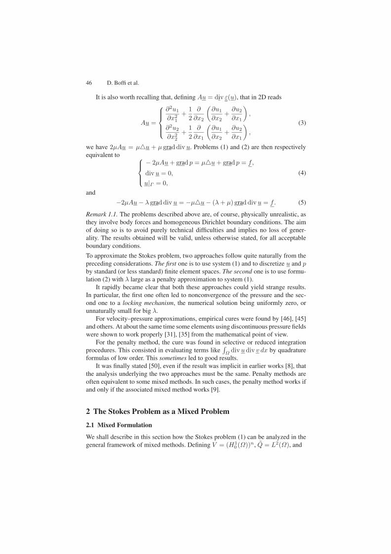
It is also worth recalling that, defining Au = div ε(u), that in 2D reads
Au =
⎧⎪⎪⎨
⎪⎪⎩
∂2u1
∂x21
+12
∂
∂x2
(∂u1
∂x2+
∂u2
∂x1
),
∂2u2
∂x22
+12
∂
∂x1
(∂u1
∂x2+
∂u2
∂x1
),
(3)
we have 2µAu = µu + µ grad div u. Problems (1) and (2) are then respectivelyequivalent to ⎧
⎪⎨
⎪⎩
− 2µAu + grad p = µu + grad p = f,
div u = 0,u|Γ = 0,
(4)
and−2µAu− λ grad div u = −µu− (λ + µ) grad div u = f. (5)
Remark 1.1. The problems described above are, of course, physically unrealistic, asthey involve body forces and homogeneous Dirichlet boundary conditions. The aimof doing so is to avoid purely technical difficulties and implies no loss of gener-ality. The results obtained will be valid, unless otherwise stated, for all acceptableboundary conditions.
To approximate the Stokes problem, two approaches follow quite naturally from thepreceding considerations. The first one is to use system (1) and to discretize u and pby standard (or less standard) finite element spaces. The second one is to use formu-lation (2) with λ large as a penalty approximation to system (1).
It rapidly became clear that both these approaches could yield strange results.In particular, the first one often led to nonconvergence of the pressure and the sec-ond one to a locking mechanism, the numerical solution being uniformly zero, orunnaturally small for big λ.
For velocity–pressure approximations, empirical cures were found by [46], [45]and others. At about the same time some elements using discontinuous pressure fieldswere shown to work properly [31], [35] from the mathematical point of view.
For the penalty method, the cure was found in selective or reduced integrationprocedures. This consisted in evaluating terms like
∫Ω
div u div v dx by quadratureformulas of low order. This sometimes led to good results.
It was finally stated [50], even if the result was implicit in earlier works [8], thatthe analysis underlying the two approaches must be the same. Penalty methods areoften equivalent to some mixed methods. In such cases, the penalty method works ifand only if the associated mixed method works [9].
2 The Stokes Problem as a Mixed Problem
2.1 Mixed Formulation
We shall describe in this section how the Stokes problem (1) can be analyzed in thegeneral framework of mixed methods. Defining V = (H1
0 (Ω))n, Q = L2(Ω), and
Finite Elements for the Stokes Problem 47
a(u, v) = 2µ∫
Ω
ε(u) : ε(v) dx, (6)
b(v, q) = −∫
Ω
q div v dx, (7)
problem (1) can clearly be written in the form: find u ∈ V and p ∈ Q such that
a(u, v) + b(v, p) = (f, v), ∀v ∈ V,
b(u, q) = 0, ∀q ∈ Q,(8)
which is a mixed problem. Indeed, it can be observed that p is the Lagrange multiplierassociated with the incompressibility constraint.
Remark 2.1. It is apparent, from the definition (7) of b(·, ·) and from the boundaryconditions of the functions in V , that p, if exists, is defined up to a constant. There-fore, we introduce the space
Q = L2(Ω)/R, (9)
where two elements q1, q2 ∈ L2(Ω) are identified if their difference is constant. Itis not difficult to show that Q is isomorphic to the subspace of L2(Ω) consisting offunctions with zero mean value on Ω.
With this choice, our problem reads: find u ∈ V and p ∈ Q such that
a(u, v) + b(v, p) = (f, v), ∀v ∈ V,
b(u, q) = 0, ∀q ∈ Q.(10)
Let us check that our problem is well-posed. With standard procedure, we canintroduce the following operators
B = −div : (H10 (Ω))n → L2(Ω)/R (11)
andBt = grad : L2(Ω)/R → (H−1(Ω))n. (12)
It can be shown (see, e.g., [64]) that
ImB = Q ∼=q ∈ L2(Ω) :
∫
Ω
q dx = 0
, (13)
hence the operator B has a continuous lifting, and the continuous inf–sup conditionis fulfilled. We also notice that, with our definition of the space Q, the kernel kerBt
reduces to zero.The bilinear form a(·, ·) is coercive on V (see [32, 64]), whence the ellipticity in
the kernel also will follow (i.e., A is invertible on kerB).
48 D. Boffi et al.
We state the well-posedness of problem (10) in the following theorem.
Theorem 2.1. Let f be given in (H−1(Ω))n. Then there exists a unique (u, p) ∈V ×Q solution to problem (10) which satisfies
||u||V + ||p||Q ≤ C||f ||H−1 . (14)
Now choosing an approximation Vh ⊂ V and Qh ⊂ Q yields the discrete problem⎧⎪⎪⎨
⎪⎪⎩
2µ∫
Ω
ε(uh) : ε(vh) dx−∫
Ω
ph div vh dx =∫
Ω
f · vhdx, ∀vh ∈ Vh,
∫
Ω
qh div uh dx = 0, ∀qh ∈ Qh.
(15)
The bilinear form a(·, ·) is coercive on V ; hence, according to the general theory ofmixed approximations, there is no problem for the existence of a solution uh, phto problem (15), while we might have troubles with the uniqueness of ph. We thustry to obtain estimates of the errors ||u− uh||V and ||p− ph||Q.
First we observe that, in general, the discrete solution uh needs not bedivergence-free. Indeed, the bilinear form b(·, ·) defines a discrete divergenceoperator
Bh = −divh : Vh → Qh. (16)
(It is convenient here to identify Q = L2(Ω)/R and Qh ⊂ Q with their dual spaces).In fact, we have
(divh uh, qh)Q =∫
Ω
qh div uh dx, (17)
and, thus, divh uh turns out to be the L2-projection of div uh onto Qh.The discrete divergence operator coincides with the standard divergence oper-
ator if div Vh ⊂ Qh. Referring to the abstract setting, we see that obtaining errorestimates requires a careful study of the properties of the operator Bh = −divh andof its transpose that we denote by gradh.
The first question is to characterize the kernel kerBth = ker(gradh). It might
happen that kerBth contains nontrivial functions In these cases ImBh = Im(divh)
will be strictly smaller than Qh = PQh(ImB); this may lead to pathologies. In par-
ticular, if we consider a modified problem, like the one that usually originates whendealing with nonhomogeneous boundary conditions, the strict inclusion ImBh ⊂ Qh
may even imply troubles with the existence of the solution. This situations is madeclearer with the following example.
Example 2.1. Let us consider problem (4) with nonhomogeneous boundary condi-tions, that is let r be such that
u|Γ = r,
∫
Γ
r · nds = 0, (18)
It is classical to reduce this case to a problem with homogeneous boundary conditionsby first introducing a function u ∈ (H1(Ω))n such that u|Γ = r. Setting u = u0 + uwith u0 ∈ (H1
0 (Ω))n we have to solve
Finite Elements for the Stokes Problem 49
− 2µAu0 + grad p = f + 2µAu = f ,
div u0 = −div u = g, u0|Γ = 0(19)
with A defined in (3). We thus find a problem with a constraint Bu0 = g whereg = 0. It may happen that the associated discrete problem fails to have a solution,because gh = PQh
g does not necessarily belongs to ImBh, whenever kerBth ⊂
kerBt. Discretization where ker(gradh) is nontrivial can therefore lead to ill-posedproblems in particular for some nonhomogeneous boundary conditions. Examples ofsuch conditions can be found in [56, 57]. In general, any method that relies on extracompatibility conditions is a source of trouble when applied to more complicated(nonlinear, time-dependent, etc.) problems.
Let us now turn our attention to the study of the error estimates. Since the bilinearform a(·, ·) is coercive on V , we only have to deal with the inf–sup condition. Thefollowing proposition will be the starting point for the analysis of any finite elementapproximation of (10).
Proposition 2.1. Let (u, p) ∈ V ×Q be the solution of (10) and suppose the follow-ing inf–sup condition holds true (with k0 independent of h)
infqh∈Qh
supvh∈Vh
∫Ωqh div vh dx
||qh||Q||vh||V≥ kh ≥ k0 > 0. (20)
Then there exists a unique (uh, ph) ∈ Vh × Qh solution to (15) and the followingestimate holds
||u− uh||V + ||p− ph||Q ≤ C infvh∈Vh, qh∈Qh
||u− vh||V + ||p− qh||Q . (21)
Remark 2.2. Actually, as it has been already observed, the existence of the discretesolution (uh, ph) (when the right-hand side in the second equation of (10) is zero)is not a consequence of the inf–sup condition (20). However, we should not forgetabout the possible situation presented in Example 2.1.
Remark 2.3. We shall also meet cases in which the constant kh is not bounded belowby k0. We shall then try to know precisely how it depends on h and to see whethera lower-order convergence can be achieved. When ker(gradh) is nontrivial, we areinterested in a weaker form of (20)
supvh∈Vh
∫Ωqh div vh dx
||vh||V≥ kh inf
q∈ker(gradh)||qh − q||L2(Ω), (22)
and in the dependence of kh in terms of h.
Several ways have also been proposed to get a more direct and intuitive evalua-tion of how a finite element scheme can approximate divergence-free functions. Oneof them is the constraint ratio, that we denote by Cr, and which is defined as
50 D. Boffi et al.
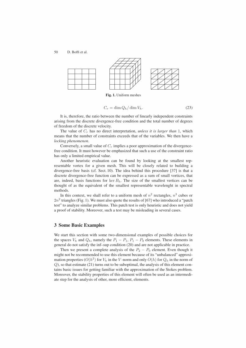
Fig. 1. Uniform meshes
Cr = dimQh/dimVh. (23)
It is, therefore, the ratio between the number of linearly independent constraintsarising from the discrete divergence-free condition and the total number of degreesof freedom of the discrete velocity.
The value of Cr has no direct interpretation, unless it is larger than 1, whichmeans that the number of constraints exceeds that of the variables. We then have alocking phenomenon.
Conversely, a small value of Cr implies a poor approximation of the divergence-free condition. It must however be emphasized that such a use of the constraint ratiohas only a limited empirical value.
Another heuristic evaluation can be found by looking at the smallest rep-resentable vortex for a given mesh. This will be closely related to building adivergence-free basis (cf. Sect. 10). The idea behind this procedure [37] is that adiscrete divergence-free function can be expressed as a sum of small vortices, thatare, indeed, basis functions for kerBh. The size of the smallest vertices can bethought of as the equivalent of the smallest representable wavelenght in spectralmethods.
In this context, we shall refer to a uniform mesh of n2 rectangles, n3 cubes or2n2 triangles (Fig. 1). We must also quote the results of [67] who introduced a “patchtest” to analyze similar problems. This patch test is only heuristic and does not yielda proof of stability. Moreover, such a test may be misleading in several cases.
3 Some Basic Examples
We start this section with some two-dimensional examples of possible choices forthe spaces Vh and Qh, namely the P1 − P1, P1 − P0 elements. These elements ingeneral do not satisfy the inf–sup condition (20) and are not applicable in practice.
Then we present a complete analysis of the P2 − P0 element. Even though itmight not be recommended to use this element because of its “unbalanced” approxi-mation properties (O(h2) for Vh in the V -norm and only O(h) for Qh in the norm ofQ), so that estimate (21) turns out to be suboptimal, the analysis of this element con-tains basic issues for getting familiar with the approximation of the Stokes problem.Moreover, the stability properties of this element will often be used as an intermedi-ate step for the analysis of other, more efficient, elements.
Finite Elements for the Stokes Problem 51
Example 3.1. The P1 − P1 elementLet us consider a very simple case, that is, a P1 continuous interpolation for both
velocity and pressure, namely, using the notation of [24],
Vh = (L11)
2 ∩ V, Qh = L11 ∩Q. (24)
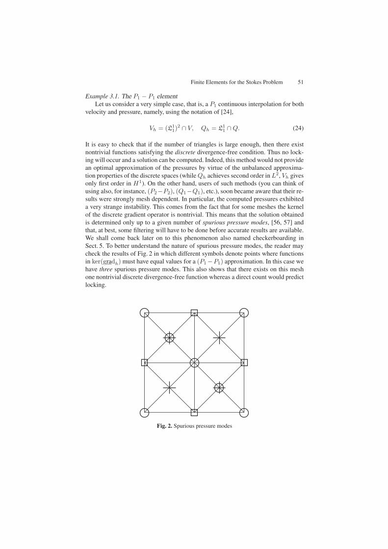
It is easy to check that if the number of triangles is large enough, then there existnontrivial functions satisfying the discrete divergence-free condition. Thus no lock-ing will occur and a solution can be computed. Indeed, this method would not providean optimal approximation of the pressures by virtue of the unbalanced approxima-tion properties of the discrete spaces (while Qh achieves second order in L2, Vh givesonly first order in H1). On the other hand, users of such methods (you can think ofusing also, for instance, (P2−P2), (Q1−Q1), etc.), soon became aware that their re-sults were strongly mesh dependent. In particular, the computed pressures exhibiteda very strange instability. This comes from the fact that for some meshes the kernelof the discrete gradient operator is nontrivial. This means that the solution obtainedis determined only up to a given number of spurious pressure modes, [56, 57] andthat, at best, some filtering will have to be done before accurate results are available.We shall come back later on to this phenomenon also named checkerboarding inSect. 5. To better understand the nature of spurious pressure modes, the reader maycheck the results of Fig. 2 in which different symbols denote points where functionsin ker(gradh) must have equal values for a (P1 −P1) approximation. In this case wehave three spurious pressure modes. This also shows that there exists on this meshone nontrivial discrete divergence-free function whereas a direct count would predictlocking.
Fig. 2. Spurious pressure modes
52 D. Boffi et al.
Example 3.2. P1 − P0 approximationThis is probably the simplest element one can imagine for the approximation of
an incompressible flow: one uses a standard P1 approximation for the velocities anda piecewise constant approximation for the pressures. With the notation of [24] thiswould read
Vh = (L11)
2 ∩ V, Qh = L00 ∩Q. (25)
As the divergence of a P1 velocity field is piecewise constant, this would lead to adivergence-free approximation. Moreover, this would give a well-balanced O(h) ap-proximation in estimate (21).
However, it is easy to see that such an element will not work for a generalmesh. Indeed, consider a triangulation of a (simply connected) domain Ω and letus denote by
— t the number of triangles,— vI the number of internal vertices,— vB the number of boundary vertices.
We shall thus have 2vI degrees of freedom (d.o.f.) for the space Vh (since the ve-locities vanish on the boundary) and (t− 1) d.o.f. for Qh (because of the zero meanvalue of the pressures) leading to (t − 1) independent divergence-free constraints.By Euler’s relations, we have
t = 2vI + vB − 2 (26)
and thust− 1 > 2vI (27)
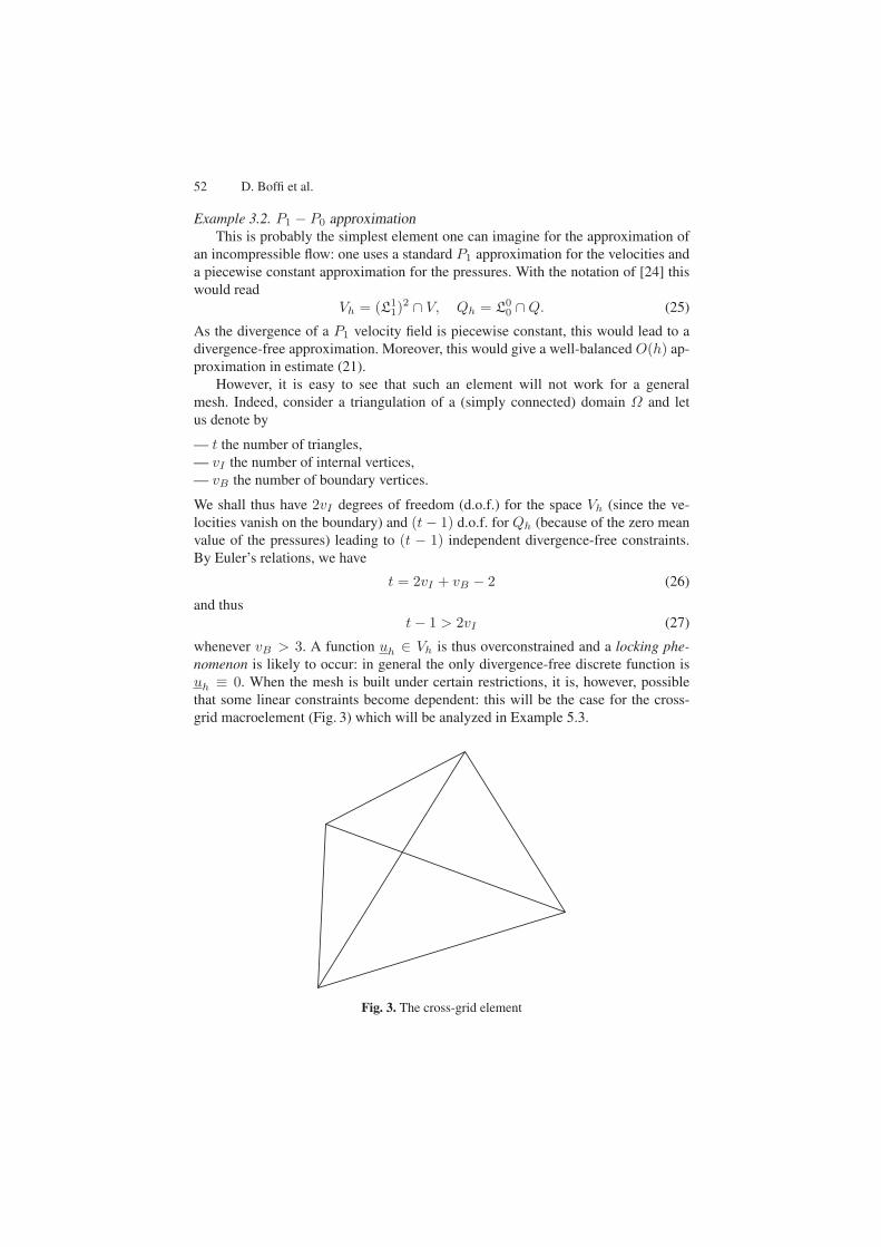
whenever vB > 3. A function uh ∈ Vh is thus overconstrained and a locking phe-nomenon is likely to occur: in general the only divergence-free discrete function isuh ≡ 0. When the mesh is built under certain restrictions, it is, however, possiblethat some linear constraints become dependent: this will be the case for the cross-grid macroelement (Fig. 3) which will be analyzed in Example 5.3.
Fig. 3. The cross-grid element
Finite Elements for the Stokes Problem 53
Example 3.3. A stable approximation: the P2 − P0 elementLet us now move to the stable P2 − P0 element; namely, we use continuous
piecewise quadratic vectors for the approximation of the velocities and piecewiseconstants for the pressures.
The discrete divergence-free condition can then be written as∫
K
div uh dx =∫
∂K
uh · nds = 0, ∀K ∈ Th, (28)
that is as a conservation of mass on every element. This is intuitively an approxi-mation of div uh = 0, directly related to the physical meaning of this condition.It is clear from error estimate (21) and standard approximation results that such anapproximation will lead to the loss of one order of accuracy due to the poor approxi-mation of the pressures. However, an augmented Lagrangian technique can be used,in order to recover a part of the accuracy loss (see Remark 3.2).
We are going to prove the following proposition.
Proposition 3.1. The choice
Vh = (L12)
2 ∩ V, Qh = L00 ∩Q (29)
fulfills the inf–sup condition (20).
Proof. Before giving the rigorous proof of Proposition 3.1 we are going to sketch themain argument.
If we try to check the inf–sup condition by building a Fortin operator Πh, then,given u, we have to build uh = Πhu such that
∫
Ω
div(u− uh)qh dx = 0, ∀qh ∈ Qh. (30)
Since qh is constant on every element K ∈ Th, this is equivalent to∫
K
div(u− uh) dx =∫
∂K
(u− uh) · nds = 0. (31)
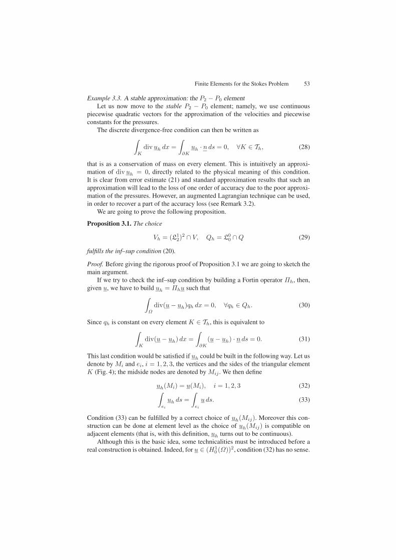
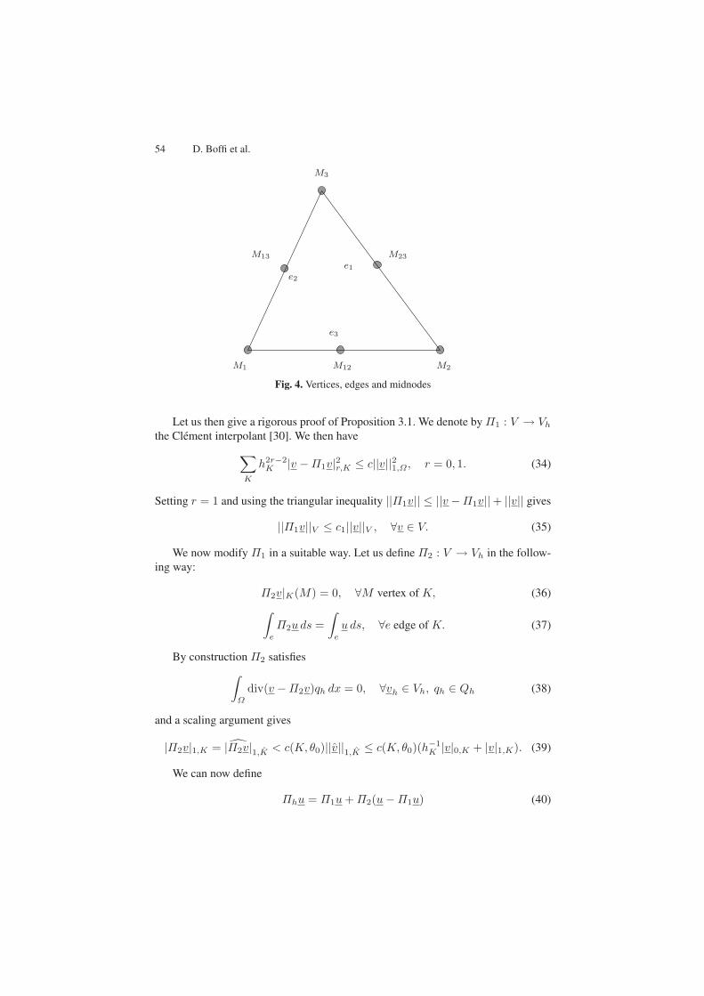
This last condition would be satisfied if uh could be built in the following way. Let usdenote by Mi and ei, i = 1, 2, 3, the vertices and the sides of the triangular elementK (Fig. 4); the midside nodes are denoted by Mij . We then define
uh(Mi) = u(Mi), i = 1, 2, 3 (32)∫
ei
uh ds =∫
ei
u ds. (33)
Condition (33) can be fulfilled by a correct choice of uh(Mij). Moreover this con-struction can be done at element level as the choice of uh(Mij) is compatible onadjacent elements (that is, with this definition, uh turns out to be continuous).
Although this is the basic idea, some technicalities must be introduced before areal construction is obtained. Indeed, for u ∈ (H1
0 (Ω))2, condition (32) has no sense.
54 D. Boffi et al.
M1 M2
M3
M12
M23M13
e1
e2
e3
Fig. 4. Vertices, edges and midnodes
Let us then give a rigorous proof of Proposition 3.1. We denote by Π1 : V → Vh
the Clement interpolant [30]. We then have∑
K
h2r−2K |v −Π1v|2r,K ≤ c||v||21,Ω , r = 0, 1. (34)
Setting r = 1 and using the triangular inequality ||Π1v|| ≤ ||v −Π1v||+ ||v|| gives
||Π1v||V ≤ c1||v||V , ∀v ∈ V. (35)
We now modify Π1 in a suitable way. Let us define Π2 : V → Vh in the follow-ing way:
Π2v|K(M) = 0, ∀M vertex of K, (36)∫
e
Π2u ds =∫
e
u ds, ∀e edge of K. (37)
By construction Π2 satisfies∫
Ω
div(v −Π2v)qh dx = 0, ∀vh ∈ Vh, qh ∈ Qh (38)
and a scaling argument gives
|Π2v|1,K = |Π2v|1,K < c(K, θ0)||v||1,K ≤ c(K, θ0)(h−1K |v|0,K + |v|1,K). (39)
We can now define
Πhu = Π1u + Π2(u−Π1u) (40)
Finite Elements for the Stokes Problem 55
M1
M12
M2
M23
M3
M13
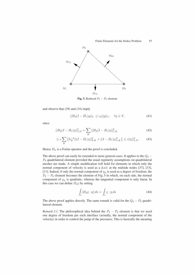
Fig. 5. Reduced P2 − P0 element
and observe that (39) and (34) imply
||Π2(I −Π1)u||V ≤ c2||u||V , ∀v ∈ V, (41)
since
||Π2(I −Π1)v||21,Ω =∑
K
||Π2(I −Π1)v||21,K (42)
≤ c∑
K
h−2
K ||(I −Π1)v||20,K + |(I −Π1)v|21,K
≤ c||v||21,Ω . (43)
Hence Πh is a Fortin operator and the proof is concluded.
The above proof can easily be extended to more general cases. It applies to the Q2 −P0 quadrilateral element provided the usual regularity assumptions on quadrilateralmeshes are made. A simple modification will hold for elements in which only thenormal component of velocity is used as a d.o.f. at the midside nodes [37], [33],[11]. Indeed, if only the normal component of uh is used as a degree of freedom, theP2 − P0 element becomes the element of Fig. 5 in which, on each side, the normalcomponent of uh is quadratic, whereas the tangential component is only linear. Inthis case we can define Π2v by setting
∫
e
(Π2v · n) ds =∫
e
v · nds (44)
The above proof applies directly. The same remark is valid for the Q2 − P0 quadri-lateral element.
Remark 3.1. The philosophical idea behind the P2 − P0 element is that we needone degree of freedom per each interface (actually, the normal component of thevelocity) in order to control the jump of the pressures. This is basically the meaning
56 D. Boffi et al.
of the Green’s formula (31). For three-dimensional elements, for instance, we wouldneed some midface node instead of a midside node in order to control the normalflux from one element to the other.
In particular, we point out that adding internal degrees of freedom to the veloc-ity space cannot stabilize elements with piecewise constant pressures which do notsatisfy the inf–sup condition.
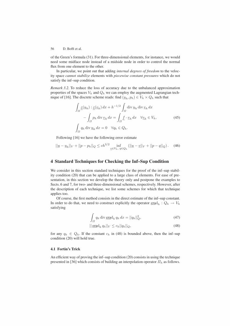
Remark 3.2. To reduce the loss of accuracy due to the unbalanced approximationproperties of the spaces Vh and Qh we can employ the augmented Lagrangian tech-nique of [16]. The discrete scheme reads: find (uh, ph) ∈ Vh ×Qh such that
∫
Ω
ε(uh) : ε(vh) dx + h−1/2
∫
Ω
div uh div vh dx
−∫
Ω
ph div vh dx =∫
Ω
f · vh dx ∀vh ∈ Vh,
∫
Ω
qh div uh dx = 0 ∀qh ∈ Qh.
(45)
Following [16] we have the following error estimate
||u− uh||V + ||p− ph||Q ≤ ch3/2 infv∈Vh, q∈Qh
(||u− v||V + ||p− q||Q) . (46)
4 Standard Techniques for Checking the Inf–Sup Condition
We consider in this section standard techniques for the proof of the inf–sup stabil-ity condition (20) that can be applied to a large class of elements. For ease of pre-sentation, in this section we develop the theory only and postpone the examples toSects. 6 and 7, for two- and three-dimensional schemes, respectively. However, afterthe description of each technique, we list some schemes for which that techniqueapplies too.
Of course, the first method consists in the direct estimate of the inf–sup constant.In order to do that, we need to construct explicitly the operator gradh : Qh → Vh
satisfying∫
Ω
qh div gradh qh dx = ||qh||2Q, (47)
|| gradh qh||V ≤ ch||qh||Q, (48)
for any qh ∈ Qh. If the constant ch in (48) is bounded above, then the inf–supcondition (20) will hold true.
4.1 Fortin’s Trick
An efficient way of proving the inf–sup condition (20) consists in using the techniquepresented in [36] which consists of building an interpolation operator Πh as follows.
Finite Elements for the Stokes Problem 57
Proposition 4.1. If there exists a linear operator Πh : V → Vh such that∫
Ω
div(u−Πhu)qh dx = 0, ∀v ∈ V, qh ∈ Qh, (49)
||Πhu||V ≤ c||u||V . (50)
then the inf–sup condition (20) holds true.
Remark 4.1. Condition (49) is equivalent to ker(gradh) ⊂ ker(grad). An elementwith this property will present no spurious pressure modes.
In several cases the operator Πh can be constructed in two steps as it has been donefor the P2–P0 element in Proposition 3.1. In general it will be enough to build twooperators Π1,Π2 ∈ L(V, Vh) such that
||Π1v||V ≤ c1||v||V , ∀v ∈ V, (51)||Π2(I −Π1)v||V ≤ c2||v||V , ∀v ∈ V, (52)∫
Ω
div(v −Π2v)qh = 0, ∀v ∈ V, ∀qh ∈ Qh, (53)
where the constants c1 and c2 are independent of h. Then the operator Πh satisfy-ing (49) and (50) will be found as
Πhu = Π1u + Π2(u−Π1u). (54)
In many cases, Π1 will be the Clement operator of [30] defined in H1(Ω).On the contrary, the choice of Π2 will vary from one case to the other, according
to the choice of Vh and Qh. However, the common feature of the various choices forΠ2 will be the following one: the operator Π2 is constructed on each element K inorder to satisfy (53). In many cases it will be such that
||Π2v||1,K ≤ c(h−1K ||v||0,K + |v|1,K). (55)
We can summarize this results in the following proposition.
Proposition 4.2. Let Vh be such that a “Clement’s operator”: Π1 : V → Vh existsand satisfies (34). If there exists an operator Π2 : V → Vh such that (53) and (55)hold, then the operator Πh defined by (54) satisfies (49) and (50) and therefore thediscrete inf–sup condition (20) holds.
Example 4.1. The construction of Fortin’s operator has been used, for instance, forthe sability proof of the P2 − P0 element (see Example 3.3).
4.2 Projection onto Constants
Following [19] we now consider a modified inf–sup condition.
infqh∈Qh
supv
h∈Vh
∫Ωqh div vh dx
||vh||V ||qh − qh||Q≥ k0 > 0, (56)
where qh is the L2-projection of qh onto L00 (that is, piecewise constant functions).
58 D. Boffi et al.
Proposition 4.3. Let us suppose that the modified inf–sup condition (56) holds withk0 independent of h. Assume moreover that Vh is such that, for any qh ∈ L0
0 ∩Q,
supv
h∈Vh
∫Ωqh div vh dx
||vh||V≥ γ0||qh||Q, (57)
with γ0 independent of h. Then the inf–sup condition (20) holds true.
Proof. For any qh ∈ Qh one has
supvh∈Vh
b(vh, qh)||vh||V
= supvh∈Vh
b(vh, qh − qh)
||vh||V+
b(vh, qh)||vh||V
≥ supv
h∈Vh
b(vh, qh)||vh||V
− supv
h∈Vh
b(vh, qh − qh)||vh||V
≥ γ0||qh||Q − ||qh − qh||0,
(58)
which implies
supvh∈Vh
b(vh, qh)||vh||V
≥ k0γ0
1 + k0||qh||Q. (59)
Putting together (56) and (59) proves the proposition.
Remark 4.2. In the case of continous pressures schemes, hypothesis (57) can be re-placed with the following approximation assumption: for any v ∈ V there existsvI ∈ Vh such that
||v − vI ||L2(Ω) ≤ c1h||v||V , ||vI ||V ≤ c2||v||V . (60)
The details of the proof can be found in [19] when the mesh is quasiuniform. Thequasiuniformity assumption is actually not needed, as it can be shown with an ar-gument similar to the one which will be presented in the next subsection (see, inparticular, Remark 4.3).
Example 4.2. The technique presented in this section will be used, for instance, forthe stability proof of the generalized two-dimensional Hood–Taylor element (seeSect. 8.2 and Theorem 8.1).
4.3 Verfurth’s Trick
Verfurth’s trick [66] applies to continuous pressures approximations and is essen-tially based on two steps. The first step is quite general and can be summarized inthe following lemma.
Lemma 4.1. Let Ω be a bounded domain in RN with Lipschitz continuous boundary.
Let Vh ⊂ (H10 (Ω))2 = V and Qh ⊂ H1(Ω) be closed subspaces. Assume that there
exists a linear operator Π0h from V into Vh and a constant c (independent of h)
such that
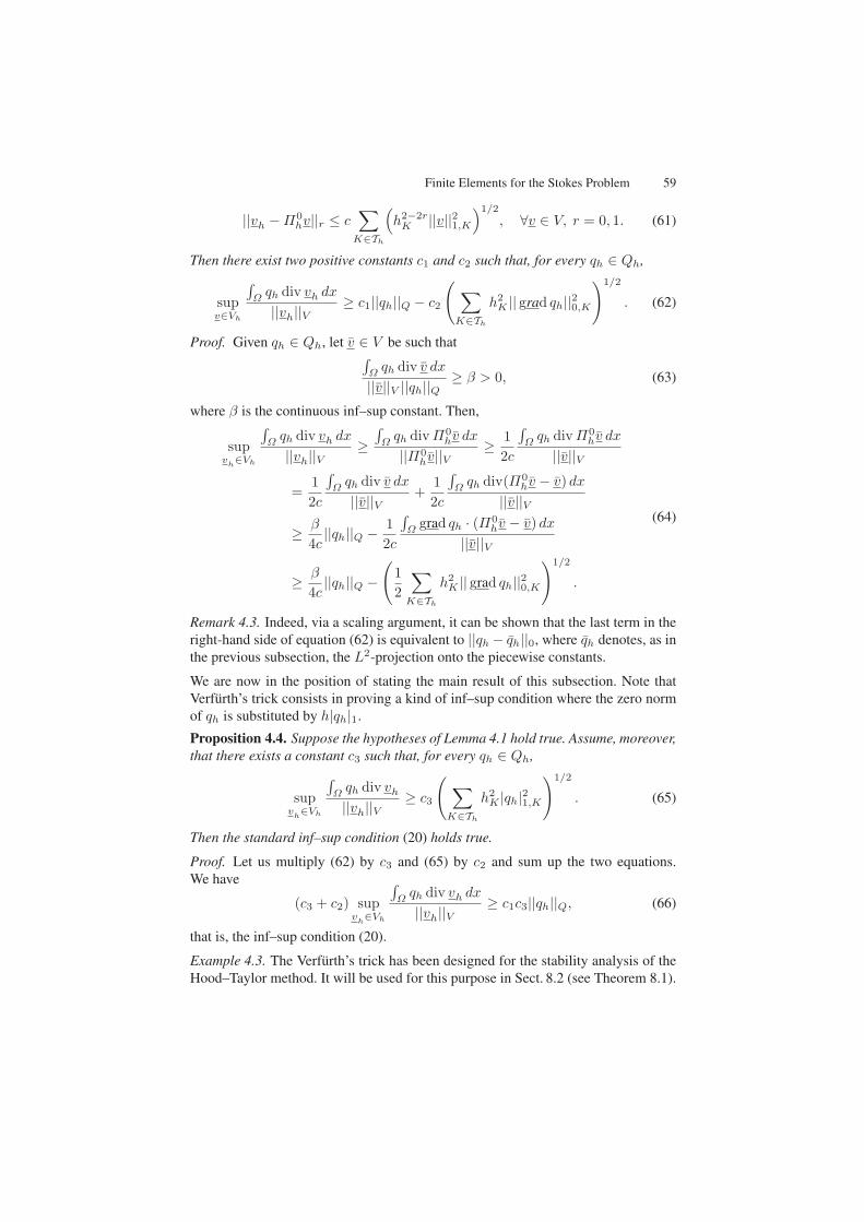
Finite Elements for the Stokes Problem 59
||vh −Π0hv||r ≤ c
∑
K∈Th
(h2−2r
K ||v||21,K
)1/2
, ∀v ∈ V, r = 0, 1. (61)
Then there exist two positive constants c1 and c2 such that, for every qh ∈ Qh,
supv∈Vh
∫Ωqh div vh dx
||vh||V≥ c1||qh||Q − c2
(∑
K∈Th
h2K || grad qh||20,K
)1/2
. (62)
Proof. Given qh ∈ Qh, let v ∈ V be such that∫
Ωqh div v dx
||v||V ||qh||Q≥ β > 0, (63)
where β is the continuous inf–sup constant. Then,
supvh∈Vh
∫Ωqh div vh dx
||vh||V≥∫
Ωqh divΠ0
hv dx
||Π0hv||V
≥ 12c
∫Ωqh divΠ0
hv dx
||v||V
=12c
∫Ωqh div v dx
||v||V+
12c
∫Ωqh div(Π0
hv − v) dx||v||V
≥ β
4c||qh||Q − 1
2c
∫Ω
grad qh · (Π0hv − v) dx
||v||V
≥ β
4c||qh||Q −
(12
∑
K∈Th
h2K || grad qh||20,K
)1/2
.
(64)
Remark 4.3. Indeed, via a scaling argument, it can be shown that the last term in theright-hand side of equation (62) is equivalent to ||qh − qh||0, where qh denotes, as inthe previous subsection, the L2-projection onto the piecewise constants.
We are now in the position of stating the main result of this subsection. Note thatVerfurth’s trick consists in proving a kind of inf–sup condition where the zero normof qh is substituted by h|qh|1.
Proposition 4.4. Suppose the hypotheses of Lemma 4.1 hold true. Assume, moreover,that there exists a constant c3 such that, for every qh ∈ Qh,
supv
h∈Vh
∫Ωqh div vh
||vh||V≥ c3
(∑
K∈Th
h2K |qh|21,K
)1/2
. (65)
Then the standard inf–sup condition (20) holds true.
Proof. Let us multiply (62) by c3 and (65) by c2 and sum up the two equations.We have
(c3 + c2) supvh∈Vh
∫Ωqh div vh dx
||vh||V≥ c1c3||qh||Q, (66)
that is, the inf–sup condition (20).
Example 4.3. The Verfurth’s trick has been designed for the stability analysis of theHood–Taylor method. It will be used for this purpose in Sect. 8.2 (see Theorem 8.1).
60 D. Boffi et al.
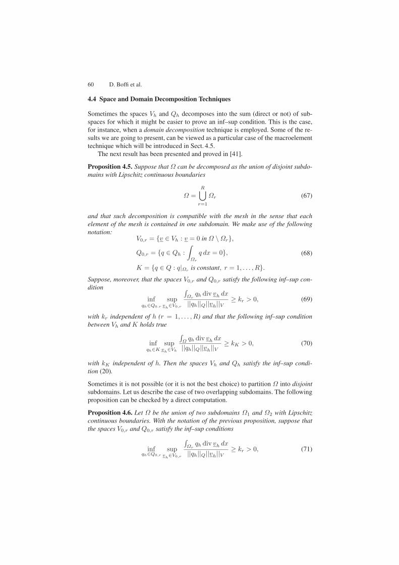
4.4 Space and Domain Decomposition Techniques
Sometimes the spaces Vh and Qh decomposes into the sum (direct or not) of sub-spaces for which it might be easier to prove an inf–sup condition. This is the case,for instance, when a domain decomposition technique is employed. Some of the re-sults we are going to present, can be viewed as a particular case of the macroelementtechnique which will be introduced in Sect. 4.5.
The next result has been presented and proved in [41].
Proposition 4.5. Suppose that Ω can be decomposed as the union of disjoint subdo-mains with Lipschitz continuous boundaries
Ω =R⋃
r=1
Ωr (67)
and that such decomposition is compatible with the mesh in the sense that eachelement of the mesh is contained in one subdomain. We make use of the followingnotation:
V0,r = v ∈ Vh : v = 0 in Ω \Ωr,
Q0,r = q ∈ Qh :∫
Ωr
q dx = 0,
K = q ∈ Q : q|Ωris constant, r = 1, . . . , R.
(68)
Suppose, moreover, that the spaces V0,r and Q0,r satisfy the following inf–sup con-dition
infqh∈Q0.r
supv
h∈V0,r
∫Ωr
qh div vh dx
||qh||Q||vh||V≥ kr > 0, (69)
with kr independent of h (r = 1, . . . , R) and that the following inf–sup conditionbetween Vh and K holds true
infqh∈K
supv
h∈Vh
∫Ωqh div vh dx
||qh||Q||vh||V≥ kK > 0, (70)
with kK independent of h. Then the spaces Vh and Qh satisfy the inf–sup condi-tion (20).
Sometimes it is not possible (or it is not the best choice) to partition Ω into disjointsubdomains. Let us describe the case of two overlapping subdomains. The followingproposition can be checked by a direct computation.
Proposition 4.6. Let Ω be the union of two subdomains Ω1 and Ω2 with Lipschitzcontinuous boundaries. With the notation of the previous proposition, suppose thatthe spaces V0,r and Q0,r satisfy the inf–sup conditions
infqh∈Q0,r
supvh∈V0,r
∫Ωr
qh div vh dx
||qh||Q||vh||V≥ kr > 0, (71)
Finite Elements for the Stokes Problem 61
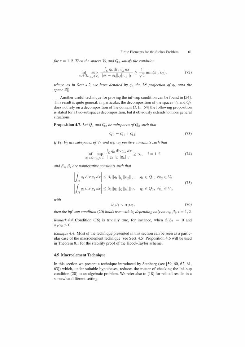
for r = 1, 2. Then the spaces Vh and Qh satisfy the condition
infqh∈Qh
supvh∈Vh
∫Ωqh div vh dx
||qh − qh||Q||vh||V≥ 1√
2min(k1, k2), (72)
where, as in Sect. 4.2, we have denoted by qh the L2 projection of qh onto thespace L0
0.
Another useful technique for proving the inf–sup condition can be found in [54].This result is quite general; in particular, the decomposition of the spaces Vh and Qh
does not rely on a decomposition of the domain Ω. In [54] the following propositionis stated for a two-subspaces decomposition, but it obviously extends to more generalsituations.
Proposition 4.7. Let Q1 and Q2 be subspaces of Qh such that
Qh = Q1 + Q2. (73)
If V1, V2 are subspaces of Vh and α1, α2 positive constants such that
infqh∈Qi
supvh∈Vi
∫Ωqh div vh dx
||qh||Q||vh||V≥ αi, i = 1, 2 (74)
and β1, β2 are nonnegative constants such that∣∣∣∣∫
Ω
q1 div v2 dx
∣∣∣∣ ≤ β1||q1||Q||v2||V , q1 ∈ Q1, ∀v2 ∈ V2,
∣∣∣∣∫
Ω
q2 div v1 dx
∣∣∣∣ ≤ β2||q2||Q||v1||V , q2 ∈ Q2, ∀v1 ∈ V1,
(75)
withβ1β2 < α1α2, (76)
then the inf–sup condition (20) holds true with k0 depending only on αi, βi, i = 1, 2.
Remark 4.4. Condition (76) is trivially true, for instance, when β1β2 = 0 andα1α2 > 0.
Example 4.4. Most of the technique presented in this section can be seen as a partic-ular case of the macroelement technique (see Sect. 4.5) Proposition 4.6 will be usedin Theorem 8.1 for the stability proof of the Hood–Taylor scheme.
4.5 Macroelement Technique
In this section we present a technique introduced by Stenberg (see [59, 60, 62, 61,63]) which, under suitable hypotheses, reduces the matter of checking the inf–supcondition (20) to an algebraic problem. We refer also to [18] for related results in asomewhat different setting.
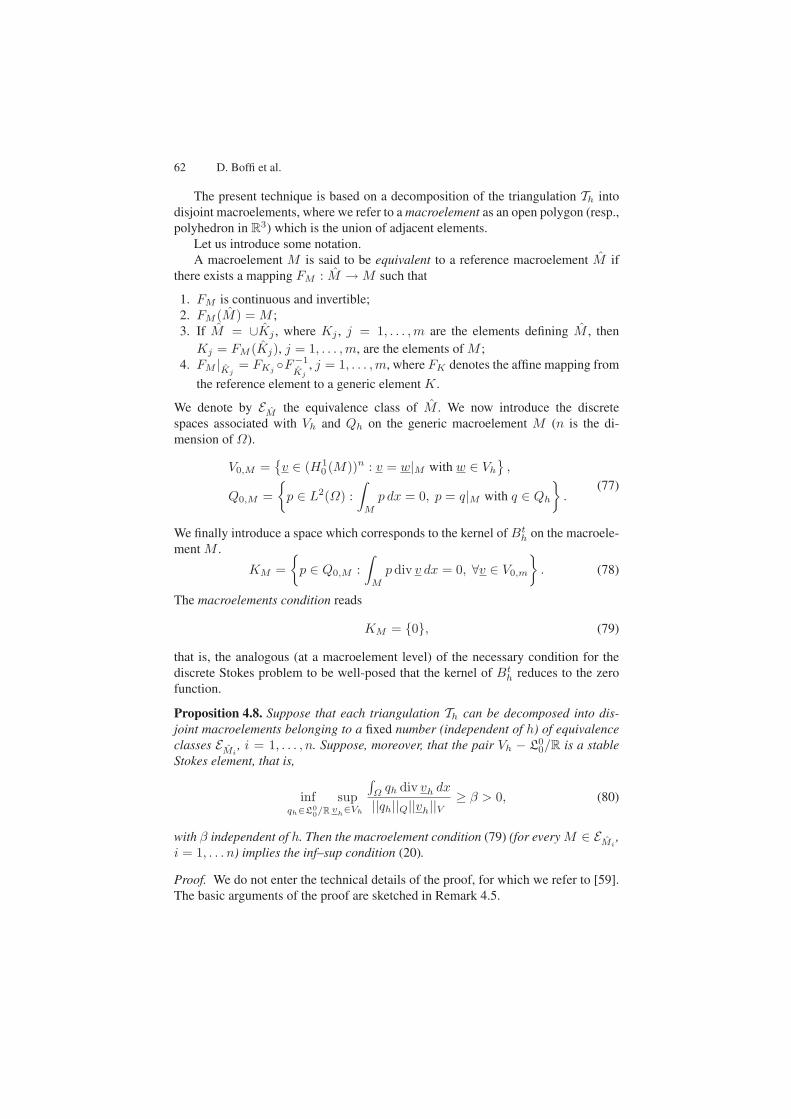
62 D. Boffi et al.
The present technique is based on a decomposition of the triangulation Th intodisjoint macroelements, where we refer to a macroelement as an open polygon (resp.,polyhedron in R
3) which is the union of adjacent elements.Let us introduce some notation.A macroelement M is said to be equivalent to a reference macroelement M if
there exists a mapping FM : M → M such that
1. FM is continuous and invertible;2. FM (M) = M ;3. If M = ∪Kj , where Kj , j = 1, . . . ,m are the elements defining M , then
Kj = FM (Kj), j = 1, . . . ,m, are the elements of M ;4. FM |Kj
= FKjF−1
Kj, j = 1, . . . ,m, where FK denotes the affine mapping from
the reference element to a generic element K.
We denote by EM the equivalence class of M . We now introduce the discretespaces associated with Vh and Qh on the generic macroelement M (n is the di-mension of Ω).
V0,M =v ∈ (H1
0 (M))n : v = w|M with w ∈ Vh
,
Q0,M =p ∈ L2(Ω) :
∫
M
p dx = 0, p = q|M with q ∈ Qh
.
(77)
We finally introduce a space which corresponds to the kernel of Bth on the macroele-
ment M .
KM =p ∈ Q0,M :
∫
M
pdiv v dx = 0, ∀v ∈ V0,m
. (78)
The macroelements condition reads
KM = 0, (79)
that is, the analogous (at a macroelement level) of the necessary condition for thediscrete Stokes problem to be well-posed that the kernel of Bt
h reduces to the zerofunction.
Proposition 4.8. Suppose that each triangulation Th can be decomposed into dis-joint macroelements belonging to a fixed number (independent of h) of equivalenceclasses EMi
, i = 1, . . . , n. Suppose, moreover, that the pair Vh − L00/R is a stable
Stokes element, that is,
infqh∈L0
0/R
supvh∈Vh
∫Ωqh div vh dx
||qh||Q||vh||V≥ β > 0, (80)
with β independent of h. Then the macroelement condition (79) (for every M ∈ EMi,
i = 1, . . . n) implies the inf–sup condition (20).
Proof. We do not enter the technical details of the proof, for which we refer to [59].The basic arguments of the proof are sketched in Remark 4.5.
Finite Elements for the Stokes Problem 63
Remark 4.5. The macroelement condition (79) is strictly related to the patch testcommonly used in the engineering practice (cf., e.g., [67]). However, the count ofthe degrees of freedom is clearly insufficient by itself. Hence, let us point out howthe hypotheses of Proposition 4.8 are important.
Hypothesis (79) (the macroelement condition) implies, via a compactness ar-gument, that a discrete inf–sup condition holds true between the spaces V0,M andQ0,M . The finite number of equivalent macroelements classes is sufficient to con-clude that the corresponding inf–sup constants are uniformly bounded below by apositive number.
Then, we are basically in the situation of the domain decomposition techniqueof Sect. 4.4. We now use hypothesis (80) to control the constant functions on eachmacroelement and to conclude the proof.
Remark 4.6. Hypothesis (80) is satisfied in the two-dimensional case whenever Vh
contains piecewise quadratic functions (see Sect. 3). In the three-dimensional casethings are not so easy (to control the constants we need extra degrees of freedomon the faces, as observed in Remark 3.1. For this reason, let us state the followingproposition which can be proved with the technique of Sect. 4.2 (see Remark 4.2)and which applies to the case of continuous pressures approximations.
Proposition 4.9. Let us make the same assumptions as in Proposition 4.8 with (80)replaced by the condition of Remark 4.2 (see (60)). Then, provided Qh ⊂ C0(Ω),the inf–sup condition (20) holds true.
Remark 4.7. The hypothesis that the macroelement partition of Th is disjoint can beweakened, in the spirit of Proposition 4.6, by requiring that each element K of Th
belongs at most to a finite number N of macroelements with N independent of h.
Example 4.5. The macroelement technique can be used in order to prove the stabilityof several schemes. Among those, we recall the Q2 − P1 element (see Sect. 6.4) andthe three-dimensional generalized Hood–Taylor scheme (see Theorem 8.2).
4.6 Making Use of the Internal Degrees of Freedom
This subsection presents a general framework providing a general tool for the analy-sis of finite element approximations to incompressible materials problems.
The basic idea has been used several times on particular cases, starting from [31]for discontinuous pressures and from [2] and [3] for continuous pressures. We aregoing to present it in its final general form given by [23]. It consists essentially instabilizing an element by adding suitable bubble functions to the velocity field.
In order to do that, we first associate to every finite element discretization Qh ⊂Q the space
B(gradQh) =β ∈ V : β|K = bK grad qh|K for some qh ∈ Qh
, (81)
where bK is a bubble function defined in K. In particular, we can take as BK the stan-dard cubic bubble if K is a triangle, or a biquadratic bubble if K is a square or other
64 D. Boffi et al.
obvious generalizations in 3D. In other words, the restriction of a β ∈ B(gradQh)to an element K is the product of the bubble functions bK times the gradient of afunction of Qh|K .
Remark 4.8. Notice that the space B(gradQh) is not defined through a basic spaceB on the reference element. This could be easily done in the case of affine elements,for all the reasonable choices of Qh. However, this is clearly unnecessary: if weknow how to compute qh on K we also know how to compute grad qh and there isno need for a reference element.
We can now prove our basic results, concerning the two cases of continuous or dis-continuous pressures.
Proposition 4.10. (Stability of continuous pressure elements). Assume that thereexists an operator Π1 ∈ L(V, Vh) satisfying the property of the Clement inter-polant (34). If Qh ⊂ C0(Ω) and Vh contains the space B(gradQh) then the pair(Vh, Qh) is a stable element, in the sense that it satisfies the inf–sup condition (20).
Proof. We shall build a Fortin operator, like in Proposition 4.2. We only need toconstruct the operator Π2. We define Π2 : V → B(gradQh), on each element, byrequiring
Π2v|K ∈ B(gradQh)|K = b3,K gradQh|K ,∫
K
(Π2v − v) · grad qh dx = 0, ∀qh ∈ Qh.(82)
Problem (82) has obviously a unique solution and Π2 satisfies (53). Finally (55)follows by a scaling argument. Hence Proposition 4.2 gives the desired result.
Corollary 4.1. Assume that Qh ⊂ Q is a space of continuous piecewise smoothfunctions. If Vh contains (L1
1)2 ⊕ B(gradQh) then the pair (Vh, Qh) satisfies the
inf–sup condition (20).
Proof. Since Vh contains piecewise linear functions, there exists a Clement inter-polant Π1 satisfying (34). Hence we can apply Proposition (4.10).
We now consider the case of discontinuous pressure elements.
Proposition 4.11. (Stability of discontinuous pressure elements). Assume that thereexists an operator Π1 ∈ L(V, Vh) satisfying
||Π1v||V ≤ c||v||V , ∀v ∈ V,∫
K
div(v − Π1v) dx = 0, ∀v ∈ V ∀K ∈ Th.(83)
If Vh contains B(gradQh) then the pair (Vh, Qh) is a stable element, in the sensethat it satisfies the inf–sup condition (20).
Finite Elements for the Stokes Problem 65
Proof. We are going to use Proposition 4.10. We take Π1 as operator Π1. We are notdefining Π2 on the whole V , but only in the subspace
V 0 =v ∈ V :
∫
K
div v dx = 0, ∀K ∈ Th
. (84)
This will be enough, since we need to apply Π2 to the difference v − Π1v which isin V 0 by (83).
For every v ∈ V 0 we define Π2v ∈ B(gradQh) by requiring that, in eachelement K,
Π2v|K ∈ B(gradQh)|K = b3,K gradQh|K ,∫
K
div(Π2v − v)qh dx = 0, ∀qh ∈ Qh|K .(85)
Note that (85) is uniquely solvable, if v ∈ V 0, since the divergence of a bubble func-tion has always zero mean value (hence the number of nontrivial equations is equalto dim(Qh|K) − 1, which is equal to the number of unknowns; the nonsingularitythen follows easily). It is obvious that Π2, as given by (85), will satisfy (53) for allv ∈ V 0. We have to check that
‖Π2v‖1 ≤ c‖v‖V , (86)
which actually follows by a scaling argument making use of the following bound
|Π2v|0,K ≤ c(θ0)|v|1,K . (87)
Corollary 4.2. (Two-dimensional case). Assume that Qh ⊂ Q is a space of piece-wise smooth functions. If Vh contains (L1
2)2 ⊕ B(gradQh) then the pair (Vh, Qh)
satisfies the inf–sup condition (20).
Proof. The stability of the P2 − P0 element (see Sect. 3 implies the existence of Π1
as in Proposition 4.11.
Propositions 4.10 and 4.11 are worth a few comments. They show that almost any el-ement can be stabilized by using bubble functions. For continuous pressure elementsthis procedure is mainly useful in the case of triangular elements. For discontinu-ous pressure elements it is possible to stabilize elements which are already stable forpiecewise constant pressure field. Examples of such a procedure can be found in [34].Stability with respect to piecewise constant pressure implies that at least one degreeof freedom on each side or face of the element is linked to the normal component ofvelocity (see [37] and Remark 3.1).
Example 4.6. The use of internal degrees of freedom can be used in the stabilityanalysis of several methods. For instance, we use it for the analysis of the MINIelement (see Sects. 6.1 and 7.1) in the case of continuous pressures and of theCrouzeix–Raviart element (see Remark 6.1 and Sect. 7.2) in the case of discontin-uous pressures.
66 D. Boffi et al.
5 Spurious Pressure Modes
For a given choice of Vh and Qh, the space Sh of spurious pressure modes is definedas follows
Sh = kerBth =
qh ∈ Qh :
∫
Ω
qh div vh dx = 0 ∀vh ∈ Vh
. (88)
It is clear that a necessary condition for the validity of the inf–sup condition (20)is the absence of spurios modes, that is,
Sh = 0. (89)
In particular, if Sh is nontrivial then the solution ph to the discrete Stokes prob-lem (15) is not unique, namely ph + sh is still a solution when sh ∈ Sh.
We shall illustrate how this situation may occur with the following example.
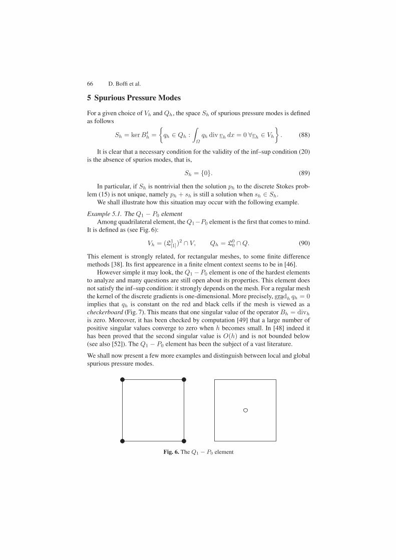
Example 5.1. The Q1 − P0 elementAmong quadrilateral element, the Q1−P0 element is the first that comes to mind.
It is defined as (see Fig. 6):
Vh = (L1[1])
2 ∩ V, Qh = L00 ∩Q. (90)
This element is strongly related, for rectangular meshes, to some finite differencemethods [38]. Its first appearence in a finite elment context seems to be in [46].
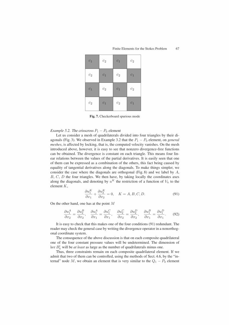
However simple it may look, the Q1 −P0 element is one of the hardest elementsto analyze and many questions are still open about its properties. This element doesnot satisfy the inf–sup condition: it strongly depends on the mesh. For a regular meshthe kernel of the discrete gradients is one-dimensional. More precisely, gradh qh = 0implies that qh is constant on the red and black cells if the mesh is viewed as acheckerboard (Fig. 7). This means that one singular value of the operator Bh = divh
is zero. Moreover, it has been checked by computation [49] that a large number ofpositive singular values converge to zero when h becomes small. In [48] indeed ithas been proved that the second singular value is O(h) and is not bounded below(see also [52]). The Q1 − P0 element has been the subject of a vast literature.
We shall now present a few more examples and distinguish between local and globalspurious pressure modes.
Fig. 6. The Q1 − P0 element
Finite Elements for the Stokes Problem 67
c1 c1
c1 c1
c1 c1
c1 c1
c2
c2
c2
c2
c2
c2
c2
c2
Fig. 7. Checkerboard spurious mode
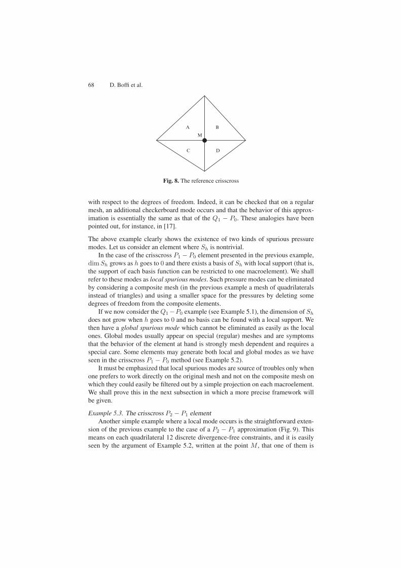
Example 5.2. The crisscross P1 − P0 elementLet us consider a mesh of quadrilaterals divided into four triangles by their di-
agonals (Fig. 3). We observed in Example 3.2 that the P1 − P0 element, on generalmeshes, is affected by locking, that is, the computed velocity vanishes. On the meshintroduced above, however, it is easy to see that nonzero divergence-free functionscan be obtained. The divergence is constant on each triangle. This means four lin-ear relations between the values of the partial derivatives. It is easily seen that oneof them can be expressed as a combination of the others, this fact being caused byequality of tangential derivatives along the diagonals. To make things simpler, weconsider the case where the diagonals are orthogonal (Fig. 8) and we label by A,B, C, D the four triangles. We then have, by taking locally the coordinates axesalong the diagonals, and denoting by uK the restriction of a function of Vh to theelement K,
∂uK1
∂x1+
∂uK2
∂x2= 0, K = A,B,C,D. (91)
On the other hand, one has at the point M
∂uA1
∂x2=
∂uB2
∂x2,
∂uA1
∂x1=
∂uC1
∂x1,
∂uC2
∂x2=
∂uD2
∂x2,
∂uB1
∂x1=
∂uD1
∂x1. (92)
It is easy to check that this makes one of the four conditions (91) redundant. Thereader may check the general case by writing the divergence operator in a nonorthog-onal coordinate system.
The consequence of the above discussion is that on each composite quadrilateralone of the four constant pressure values will be undetermined. The dimension ofkerBt
h will be at least as large as the number of quadrilaterals minus one.Thus, three constraints remain on each composite quadrilateral element. If we
admit that two of them can be controlled, using the methods of Sect. 4.6, by the “in-ternal” node M , we obtain an element that is very similar to the Q1 − P0 element
68 D. Boffi et al.
A B
C D
M
Fig. 8. The reference crisscross
with respect to the degrees of freedom. Indeed, it can be checked that on a regularmesh, an additional checkerboard mode occurs and that the behavior of this approx-imation is essentially the same as that of the Q1 − P0. These analogies have beenpointed out, for instance, in [17].
The above example clearly shows the existence of two kinds of spurious pressuremodes. Let us consider an element where Sh is nontrivial.
In the case of the crisscross P1 − P0 element presented in the previous example,dimSh grows as h goes to 0 and there exists a basis of Sh with local support (that is,the support of each basis function can be restricted to one macroelement). We shallrefer to these modes as local spurious modes. Such pressure modes can be eliminatedby considering a composite mesh (in the previous example a mesh of quadrilateralsinstead of triangles) and using a smaller space for the pressures by deleting somedegrees of freedom from the composite elements.
If we now consider the Q1−P0 example (see Example 5.1), the dimension of Sh
does not grow when h goes to 0 and no basis can be found with a local support. Wethen have a global spurious mode which cannot be eliminated as easily as the localones. Global modes usually appear on special (regular) meshes and are symptomsthat the behavior of the element at hand is strongly mesh dependent and requires aspecial care. Some elements may generate both local and global modes as we haveseen in the crisscross P1 − P0 method (see Example 5.2).
It must be emphasized that local spurious modes are source of troubles only whenone prefers to work directly on the original mesh and not on the composite mesh onwhich they could easily be filtered out by a simple projection on each macroelement.We shall prove this in the next subsection in which a more precise framework willbe given.
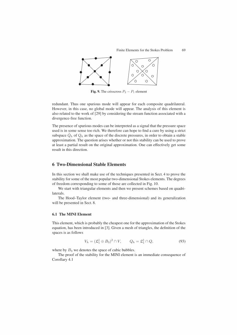
Example 5.3. The crisscross P2 − P1 elementAnother simple example where a local mode occurs is the straightforward exten-
sion of the previous example to the case of a P2 − P1 approximation (Fig. 9). Thismeans on each quadrilateral 12 discrete divergence-free constraints, and it is easilyseen by the argument of Example 5.2, written at the point M , that one of them is
Finite Elements for the Stokes Problem 69
Fig. 9. The crisscross P2 − P1 element
redundant. Thus one spurious mode will appear for each composite quadrilateral.However, in this case, no global mode will appear. The analysis of this element isalso related to the work of [29] by considering the stream function associated with adivergence-free function.
The presence of spurious modes can be interpreted as a signal that the pressure spaceused is in some sense too rich. We therefore can hope to find a cure by using a strictsubspace Qh of Qh as the space of the discrete pressures, in order to obtain a stableapproximation. The question arises whether or not this stability can be used to proveat least a partial result on the original approximation. One can effectively get someresult in this direction.
6 Two-Dimensional Stable Elements
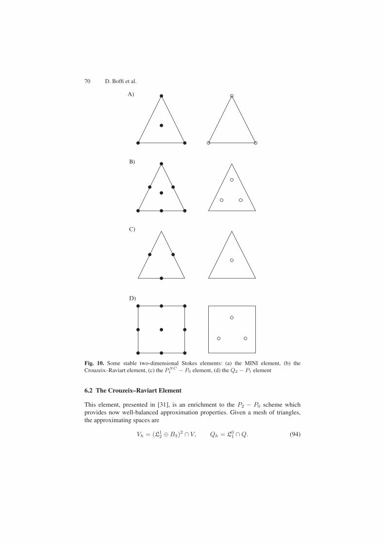
In this section we shall make use of the techniques presented in Sect. 4 to prove thestability for some of the most popular two-dimensional Stokes elements. The degreesof freedom corresponding to some of those are collected in Fig. 10.
We start with triangular elements and then we present schemes based on quadri-laterals.
The Hood–Taylor element (two- and three-dimensional) and its generalizationwill be presented in Sect. 8.
6.1 The MINI Element
This element, which is probably the cheapest one for the approximation of the Stokesequation, has been introduced in [3]. Given a mesh of triangles, the definition of thespaces is as follows
Vh = (L11 ⊕B3)2 ∩ V, Qh = L1
1 ∩Q, (93)
where by B3 we denotes the space of cubic bubbles.The proof of the stability for the MINI element is an immediate consequence of
Corollary 4.1
70 D. Boffi et al.
A)
B)
C)
D)
Fig. 10. Some stable two-dimensional Stokes elements: (a) the MINI element, (b) theCrouzeix–Raviart element, (c) the P NC
1 − P0 element, (d) the Q2 − P1 element
6.2 The Crouzeix–Raviart Element
This element, presented in [31], is an enrichment to the P2 − P0 scheme whichprovides now well-balanced approximation properties. Given a mesh of triangles,the approximating spaces are
Vh = (L12 ⊕B3)2 ∩ V, Qh = L0
1 ∩Q. (94)
Finite Elements for the Stokes Problem 71
The proof of the stability for this element can been carried out again with the help ofProposition 4.2. We use as operator Π1 the Fortin operator of the P2 − P0 element(see also Proposition 4.11) and we take advantage of the internal degrees of freedomin Vh to define Π2 : V → (B3)2. Actually, we shall define Π2v only in the casewhen div v has zero mean value in each K. This will be sufficient, since we shall usein practice Π2(v −Π1v) and Π1v satisfies (83). For all K and for all v with
∫
K
div v dx = 0, (95)
we then set Π2v as the unique solution of
Π2v ∈ (B3(K))2, (96)∫
K
div(Π2v − v)qh dx = 0, ∀qh ∈ P1(K). (97)
Note that (96), (97) is a linear system of three equations (dimP1(K) = 3) in twounknowns (dim(B3(K))2 = 2) which is compatible since v is assumed to satisfy(95) and, on the other hand, for every b ∈ (B3(K))2 we clearly have
∫
K
div b dx = 0. (98)
We have only to prove that
||Π2v||1,K ≤ c||v||1,K (99)
for all v ∈ V satisfying (95). Indeed (97) can be written as∫
K
(Π2v) · grad qh dx =∫
K
div v(qh − qh) dx (100)
where qh is any piecewise constant approximation of qh. A scaling argument yields
|Π2v|0,K ≤ c(θ0)|v|1,K (101)
that easily implies (99).
Remark 6.1. We could prove the same result also as a consequence of Proposition4.11. The same proof applies quite directly to the Q2 − P1 rectangular element (seeSect. 6.4). It can also be used to create nonstandard elements. For instance, in [34],bubble functions were added to a Q1−P0 element in order to use a P1 pressure field.This element is not more, but neither less, stable than the standard Q1−P0 and givesbetter results in some cases.
6.3 P NC1 − P0 Approximation
We consider the classical stable nonconforming triangular element introducedin [31], in which midside nodes are used as degrees of freedom for the veloci-ties. This generates a piecewise linear nonconforming approximation; pressures are
72 D. Boffi et al.
taken constant on each element (see Fig. 10). We do not present the stability analysisfor this element, which does not fit within the framework of our general results,since Vh is not contained in V . However, we remark that this method is attractive forseveral reasons. In particular, the restriction to an element K of the solution uh ∈ Vh
is exactly divergence-free, since div Vh ⊂ Qh. Another important feature of thiselement is that it can be seen as a “mass conservation” scheme. The present elementhas been generalized to second order in [39]. It must also be said that coercivenessmay be a problem for the PNC
1 − P0 element, as it does not satisfy the discreteversion of Korn’s inequality. This issue has been deeply investigated and clearlyillustrated in [5].
Remark 6.2. The generalization of nonconforming finite elements to quadrilateralsis not straightforward. In particular, approximation properties of the involved spacesare not obvious. More details can be found in [55].
6.4 Qk − Pk−1 Elements
We now discuss the stability and convergence of a familiy of quadrilateral elements.The lowest order of this family, the Q2 − P1 element, is one of the most popularStokes elements. Given k ≥ 2, the discrete spaces are defined as follows:
Vh = (L1[k])
2 ∩ V, Qh = L0[k−1] ∩Q.
If the mesh is built of rectangles, the stability proof is an immediate consequenceof Proposition 4.11, since (83) is satisfied for Vh (indeed, the Q2 − P0 is a stableStokes element, see Remark 3.1). In the case of a general quadrilateral mesh thingsare not so easy; even the definition of the space Qh is not so obvious and therehave been different opinions, during the years, about two possible natural definitions.Following [15], we discuss in detail the case k = 2.
The Q2 − P1 Element
This element was apparently discovered around a blackboard at the Banff Confer-ence on Finite Elements in Flow Problems (1979). Two different proofs of stabilitycan be found in [41] and [59] for the rectangular case. This element is a relativelylate comer in the field; the reason for this is that using a P1 pressure on a quadri-lateral is not a standard procedure. It appeared as a cure for the instability of theQ2 −Q1 element which appears quite naturally in the use of reduced integrationpenalty methods (see [9]). This last element is essentially related to the Q1 − P0
element and suffers the same problems altough to a lesser extent. Another cure canbe obtained by adding internal nodes (see [34]).
On a general quadrilateral mesh, the space Qh can be defined in two differentways: either Qh consists of (discontinuous) piecewise linear functions, or it is builtby considering three linear shape functions on the reference unit square and mappingthem to the general elements like it is usually done for continuous finite elements.We point out that, since the mapping FK from the reference element K to the general
Finite Elements for the Stokes Problem 73
element K in this case is bilinear but not affine, the two constructions are not equiv-alent. We shall refer to the first possibility as unmapped pressure approach and to thesecond one as mapped pressure approach.
In order to analyze the stability of either scheme, we use the macroelement tech-nique presented in section 4.5 with macroelements consisting of one single element.We start with the case of the unmapped pressure approach; this is the original proofpresented in [59]. Let M be a macroelement and qh = a0 + axx + ayy ∈ Q0,M
an arbitrary function in KM . If b(x, y) denote the biquadratic bubble function on K,then vh = (axb(x, y), 0) is an element of V0,M and
0 =∫
M
qh div vh dx dy = −∫
M
grad qh · vh dx dy = −ax
∫
M
b(x, y) dx dy
implies ax = 0. In a similar way, we get ay = 0 and, since the average of qh on Mvanishes, we have the macroelement condition qh = 0.
We now move to the mapped pressure approach, following the proof presentedin [15]. There, it is recalled that the macroelement condition (79) can be related toan algebraic problem in which we are led to proof that a 2× 2 matrix is nonsingular.Actually, it turns out that the determinant of such matrix is a multiple of the Jacobiandeterminant of the function mapping the reference square K onto M , evaluated atthe barycenter of K. Since this number must be nonzero for any element of a well-defined mesh, we can deduce that the macroelement condition is satisfied in this casealso, and then conclude that the stability holds thanks to Proposition 4.8.
So far, we have shown that either the unmapped and the mapped pressure ap-proach gives rise to a stable Q2 − P1 scheme. However, as a consequence of theresults proved in [6], we have that the mapped pressure approach cannot achieve op-timal approximation order. Namely, the unmapped pressure space provides a second-order convergence in L2, while the mapped one achieves only O(h) in the samenorm. In [15] several numerical experiments have been reported, showing that ongeneral quadrilateral meshes (with constant distortion) the unmapped pressure ap-proach provides a second-order convergence (for both velocity in H1 and pressurein L2), while the mapped approach is only suboptimally first-order convergent. Itis interesting to remark that in this case also the convergence of the velocities issuboptimal, according to the error estimate (21).
7 Three-Dimensional Elements
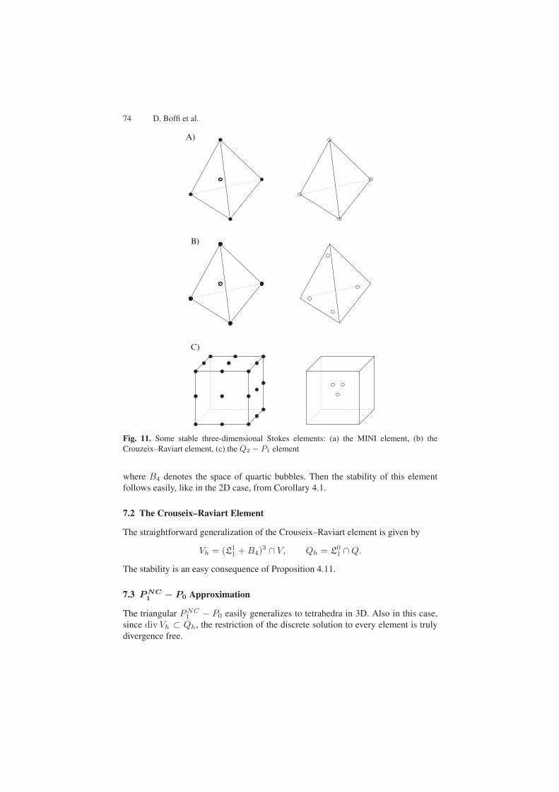
Most elements presented in Sect. 6 have a three-dimensional extension. Some ofthem are schematically plotted in Fig. 11.
7.1 The MINI Element
Consider a regular sequence of decompositions of Ω into tetrahedra. The spaces aredefined as follows:
Vh = (L11 + B4)3 ∩ V, Qh = L1
1 ∩Q,
74 D. Boffi et al.
C)
B)
A)
Fig. 11. Some stable three-dimensional Stokes elements: (a) the MINI element, (b) theCrouzeix–Raviart element, (c) the Q2 − P1 element
where B4 denotes the space of quartic bubbles. Then the stability of this elementfollows easily, like in the 2D case, from Corollary 4.1.
7.2 The Crouseix–Raviart Element
The straightforward generalization of the Crouseix–Raviart element is given by
Vh = (L11 + B4)3 ∩ V, Qh = L0
1 ∩Q.
The stability is an easy consequence of Proposition 4.11.
7.3 P NC1 − P0 Approximation
The triangular PNC1 − P0 easily generalizes to tetrahedra in 3D. Also in this case,
since div Vh ⊂ Qh, the restriction of the discrete solution to every element is trulydivergence free.
Finite Elements for the Stokes Problem 75
7.4 Qk − Pk−1 Elements
Given a mesh of hexahedrons, we define
Vh = (L1[k])
3 ∩ V, Qh = L0[k−1] ∩Q,
for k ≥ 2. We refer to the two-dimensional case (see Sect. 6.4) for the definition ofthe pressure space. In particular, we recall that Qh on each element consists of truepolynomials and is not defined via the reference element. With the correct definitionof the pressure space, the proof of stability for this element is a simple generalizationof the corresponding two-dimensional version.
8 Pk − Pk−1 Schemes and Generalized Hood–Taylor Elements
The main result of this section (see Theorems 8.1 and 8.2) consists in showing thata family of popular Stokes elements satisfies the inf–sup condition (20). The firstelement of this family has been introduced in [45] and for this reason the membersof the whole family are usually referred to as generalized Hood–Taylor elements.
This section is organized in two subsections. In the first one we discuss discon-tinuous pressure approximations for the Pk − Pk−1 element in the two-dimensionaltriangular case; it turns out that this choice is not stable in the lower-order cases andrequires suitable conditions on the mesh sequences for the stability of the higher-order elements.
The last subsection deals with the generalized Hood–Taylor elements, which pro-vide a continuous pressure approximation in the plane (triangles and quadrilaterals)and in the three-dimensional space (tetrahedrons and hexahedra).
8.1 Pk − Pk−1 Elements
In this subsection we shall recall the statement of a basic result by Scott andVogelius [58] which, roughly speaking, says: under suitable assumptions on the de-composition Th (in triangles) the pair Vh = (L1
2)2, Qh = L1
k−1 satisfies the inf–supcondition for k ≥ 4.
On the other hand, the problem of finding stable lower-order approximations hasbeen studied by Qin [54], where interesting remarks are made on this scheme andwhere the possibility of filtering out the spurious pressure modes is considered.
In order to state in a precise way the restrictions that have to be made on the tri-angulation for higher-order approximations, we assume that Ω is a polygon, and thatits boundary ∂Ω has no double points. In other words, there exists two continuouspiecewise linear maps x(t), y(t) from [0, 1[ into R such that
(x(t1) = x(t2) and y(t1) = y(t2)) implies t1 = t2,
∂Ω = (x, y) : x = x(t), y = y(t) for some t ∈ [0, 1[ .(102)
76 D. Boffi et al.
Clearly, we will have limt→1
x(t) = x(0) and limt→1
y(t) = y(0). We remark that we areconsidering a less general case than the one treated by [58]. We shall make furtherrestrictions in what follows, so that we are actually going to present a particular caseof their results.
Let now V be a vertex of a triangulation Th of Ω and let θ1, . . . , θp, be theangles, at V , of all the triangles meeting at V , ordered, for instance, in the counter-clockwise sense. If V is an internal vertex we also set θp+1 := θ1. Now we defineS(V ) according to the following rules:
p = 1 ⇒ S(V ) = 0 (103)p > 1, V ∈ ∂Ω ⇒ S(V ) = max
i=1,p−1(π − θ1 − θi+1) (104)
V /∈ ∂Ω ⇒ S(V ) = maxi=1,p
(π − θi − θi+1) (105)
It is easy to check that S(V ) = 0 if and only if all the edges of Th meeting at V fallon two straight lines. In this case V is said to be singular [58]. If S(V ) is positivebut very small, then V will be “almost singular”. Thus S(V ) measures how close Vis to be singular.
We are now able to state the following result.
Proposition 8.1 ([58]). Assume that there exists two positive constants c and δsuch that
ch ≤ hK , ∀K ∈ Th, (106)
andS(V ) ≥ δ, ∀V vertex of Th. (107)
Then the choice Vh = (L11)
2, Qh = L0k−1, k ≤ 4, satisfies the inf–sup condition
with a constant depending on c and δ but not on h.
Condition (107) is worth a few comments. The trouble is that S(V ) = 0 makes thelinear constraints on uh, arising from the divergence-free condition, linearly depen-dent (see, also, Examples 5.2 and 5.3). When this linear dependence appears, somepart of the pressure becomes unstable. In the present case, this unstable part could befiltered out.
Remark 8.1. The Pk−Pk−1 element can obviously be stabilized by adding bubbles tothe velocity space in the spirit of Sect. 4.6 (see Proposition 4.11). For a less expensivestabilization, consisting in adding bubbles only in few elements, see [13].
8.2 Generalized Hood–Taylor Elements
In this subsection we recall the results proved in [12, 14] concerning the stability ofthe generalized Hood–Taylor schemes. On triangles or tetrahedra, velocities are ap-proximated by a standard Pk element and pressures by a standard continuous Pk−1,that is vh ∈ (L1
k)n (n = 2, 3), p ∈ L1k−1. This choice has an analogue on rectangles
or cubes using a Qk element for velocities and a Qk−1 element for pressures. The
Finite Elements for the Stokes Problem 77
lowest order element (i.e., k = 2) has been introduced by Hood and Taylor [45].Several papers are devoted to the analysis of this popular element. The degrees offreedom of some elements belonging to this family are reported in Fig. 12.
The first proof of convergence was given for the two-dimensional case in [10]where a weaker form of the inf–sup condition was used. The analysis was subse-quently improved in [66] who showed that the classical inf–sup condition is indeedsatisfied (see Verfurth’s trick in Sect. 4.3). The macroelement technique can easilybe used for the stability proof of the rectangular and cubic element (of any order) aswell as of the tetrahedral case when k = 2 (see [59]). In [24] an alternative techniqueof proof has been presented for the triangular and tetrahedral cases when k = 2. Thisproof generalizes to the triangular case when k = 3 (see [21]). Finally, a generalproof of convergence can be found in [12] and [14] for the triangular and tetrahedralcase, respectively.
We now state and prove the theorem concerning the two-dimensional triangularcase (see [12]).
Theorem 8.1. Let Ω be a polygonal domain and Th a regular sequence of triangulardecompositions of it. Then the choice Vh = (L1
k∩H10 (Ω))2 and Qh = L1
k−1∩L20(Ω)
satisfies the inf–sup condition (20) for any k ≥ 2 if and only if each triangulationcontains at least three triangles.
Proof. Step 1: Necessary part. Let us show first that the hypothesis on the meshis necessary. If Th only contains one element, then it is easy to see that the inf–supconstant is zero (otherwise it should be div Vh ⊂ Qh, which is not the case since thefunctions in Qh are not zero at the vertices). We shall show that if Th contains onlytwo triangles T1 and T2, then there exists one spurious pressure mode. This impliesthat also in this case the inf–sup constant vanishes. We choose the coordinate system(x, y) in such a way that the common edge of T1 and T2 lies on the y-axis. Moreover,we suppose that T2 is the reference triangle and T1 the symmetric one with respectto the x-axis, see Fig. 13. The general case can then be handled by means of suitableaffine mappings.
We denote by λi,a and λi,b the barycentric coordinates relative to the vertices aand b, respectively, belonging to the element Ti, i = 1, 2. It is easy to check that itholds: λ1,a = 1 + x − y, λ1,b = y, λ2,a = 1 − x − y, and λ2,b = y. We shall alsomake use of the function λ2,c = x. Let L(x) be the Legendre polynomial of degreek− 2 on the unit interval with respect to the weight w(x) = x(1− x)3 and considerthe function p(x) ∈ Qh defined as follows:
p′(x) =
−L(−x) for x < 0,L(x) for x > 0.
(108)
We shall show that grad p is orthogonal to any velocity v ∈ Vh. Since p does notdepend on y, we can consider the first component v1 of v only, which, by virtue ofthe continuity at x = 0 and of the boundary conditions, has the following generalform:
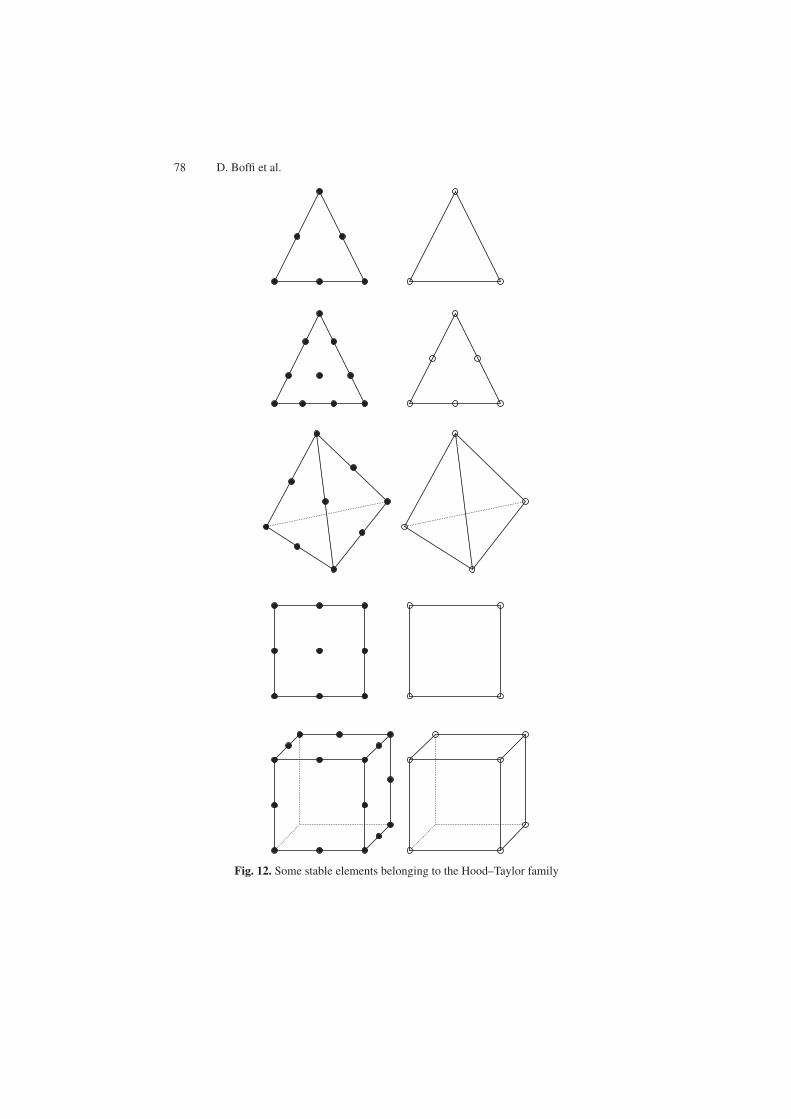
78 D. Boffi et al.
Fig. 12. Some stable elements belonging to the Hood–Taylor family
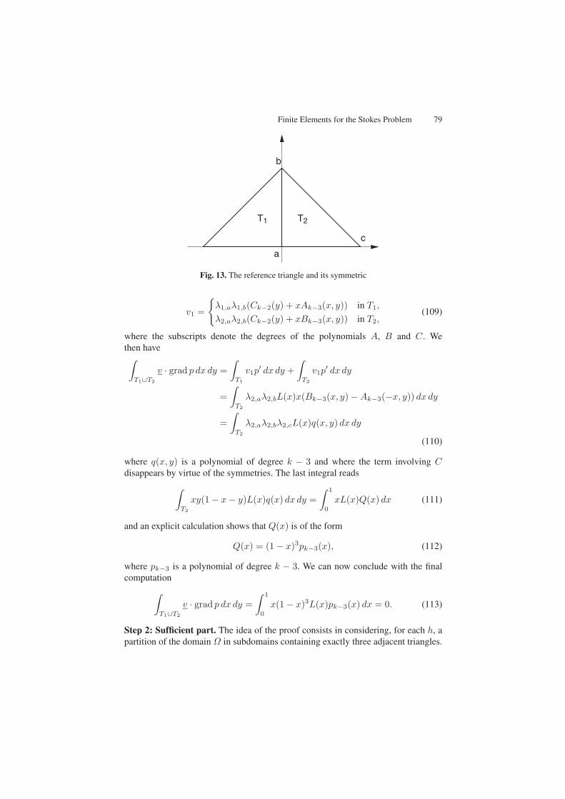
Finite Elements for the Stokes Problem 79
T1 T2
b
a
c
Fig. 13. The reference triangle and its symmetric
v1 =
λ1,aλ1,b(Ck−2(y) + xAk−3(x, y)) in T1,
λ2,aλ2,b(Ck−2(y) + xBk−3(x, y)) in T2,(109)
where the subscripts denote the degrees of the polynomials A, B and C. Wethen have∫
T1∪T2
v · grad p dx dy =∫
T1
v1p′ dx dy +
∫
T2
v1p′ dx dy
=∫
T2
λ2,aλ2,bL(x)x(Bk−3(x, y) −Ak−3(−x, y)) dx dy
=∫
T2
λ2,aλ2,bλ2,cL(x)q(x, y) dx dy
(110)
where q(x, y) is a polynomial of degree k − 3 and where the term involving Cdisappears by virtue of the symmetries. The last integral reads
∫
T2
xy(1 − x− y)L(x)q(x) dx dy =∫ 1
0
xL(x)Q(x) dx (111)
and an explicit calculation shows that Q(x) is of the form
Q(x) = (1 − x)3pk−3(x), (112)
where pk−3 is a polynomial of degree k − 3. We can now conclude with the finalcomputation
∫
T1∪T2
v · grad p dx dy =∫ 1
0
x(1 − x)3L(x)pk−3(x) dx = 0. (113)
Step 2: Sufficient part. The idea of the proof consists in considering, for each h, apartition of the domain Ω in subdomains containing exactly three adjacent triangles.
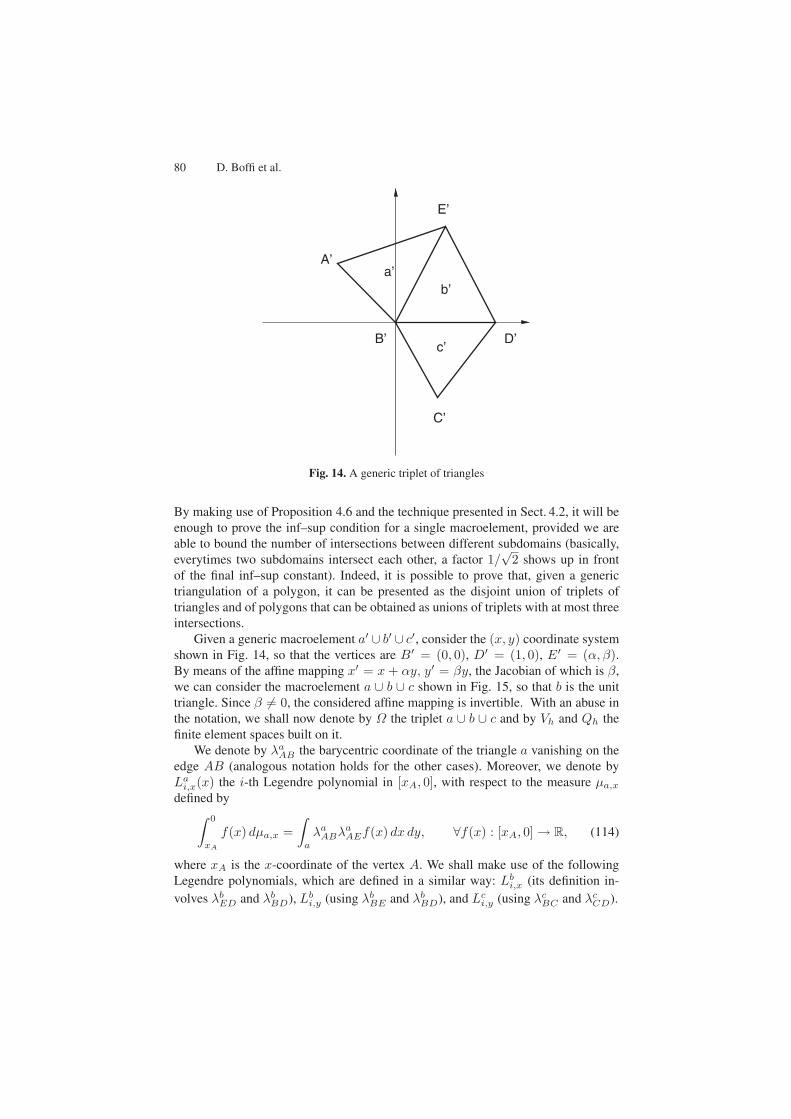
80 D. Boffi et al.
B’ D’
E’
a’b’
c’
A’
C’
Fig. 14. A generic triplet of triangles
By making use of Proposition 4.6 and the technique presented in Sect. 4.2, it will beenough to prove the inf–sup condition for a single macroelement, provided we areable to bound the number of intersections between different subdomains (basically,everytimes two subdomains intersect each other, a factor 1/
√2 shows up in front
of the final inf–sup constant). Indeed, it is possible to prove that, given a generictriangulation of a polygon, it can be presented as the disjoint union of triplets oftriangles and of polygons that can be obtained as unions of triplets with at most threeintersections.
Given a generic macroelement a′ ∪ b′ ∪ c′, consider the (x, y) coordinate systemshown in Fig. 14, so that the vertices are B′ = (0, 0), D′ = (1, 0), E′ = (α, β).By means of the affine mapping x′ = x + αy, y′ = βy, the Jacobian of which is β,we can consider the macroelement a ∪ b ∪ c shown in Fig. 15, so that b is the unittriangle. Since β = 0, the considered affine mapping is invertible. With an abuse inthe notation, we shall now denote by Ω the triplet a ∪ b ∪ c and by Vh and Qh thefinite element spaces built on it.
We denote by λaAB the barycentric coordinate of the triangle a vanishing on the
edge AB (analogous notation holds for the other cases). Moreover, we denote byLa
i,x(x) the i-th Legendre polynomial in [xA, 0], with respect to the measure µa,x
defined by∫ 0
xA
f(x) dµa,x =∫
a
λaABλa
AEf(x) dx dy, ∀f(x) : [xA, 0] → R, (114)
where xA is the x-coordinate of the vertex A. We shall make use of the followingLegendre polynomials, which are defined in a similar way: Lb
i,x (its definition in-volves λb
ED and λbBD), Lb
i,y (using λbBE and λb
BD), and Lci,y (using λc
BC and λcCD).
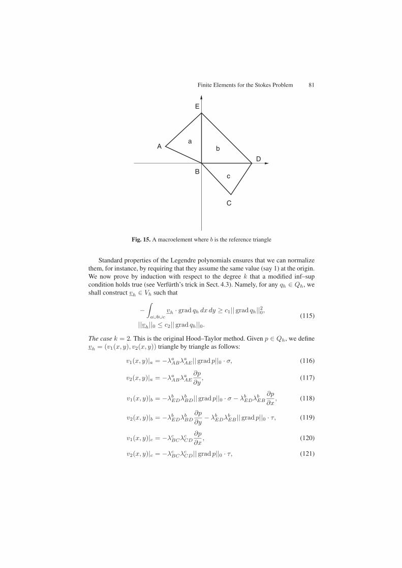
Finite Elements for the Stokes Problem 81
B
E
D
C
ab
c
A
Fig. 15. A macroelement where b is the reference triangle
Standard properties of the Legendre polynomials ensures that we can normalizethem, for instance, by requiring that they assume the same value (say 1) at the origin.We now prove by induction with respect to the degree k that a modified inf–supcondition holds true (see Verfurth’s trick in Sect. 4.3). Namely, for any qh ∈ Qh, weshall construct vh ∈ Vh such that
−∫
a∪b∪c
vh · grad qh dx dy ≥ c1|| grad qh||20,
||vh||0 ≤ c2|| grad qh||0.(115)
The case k = 2. This is the original Hood–Taylor method. Given p ∈ Qh, we definevh = (v1(x, y), v2(x, y)) triangle by triangle as follows:
v1(x, y)|a = −λaABλa
AE || grad p||0 · σ, (116)
v2(x, y)|a = −λaABλa
AE
∂p
∂y, (117)
v1(x, y)|b = −λbEDλb
BD|| grad p||0 · σ − λbEDλb
EB
∂p
∂x, (118)
v2(x, y)|b = −λbEDλb
BD
∂p
∂y− λb
EDλbEB|| grad p||0 · τ, (119)
v1(x, y)|c = −λcBCλc
CD
∂p
∂x, (120)
v2(x, y)|c = −λcBCλc
CD|| grad p||0 · τ, (121)
82 D. Boffi et al.
where the quantities σ and τ are equal to ±1 so that the expressions
H = σ|| grad p||0(∫
a
λaABλa
AE · ∂p∂x
+∫
b
λbEDλb
BD · ∂p∂x
), (122)
K = τ || grad p||0(∫
b
λbEBλb
ED · ∂p∂y
+∫
c
λcBCλc
CD · ∂p∂y
)(123)
are nonnegative. First of all, we observe that vh is an element of Vh: its degree is atmost two in each triangle, it vanishes on the boundary and it is continuous across thethe internal edges because so is the tangential derivative of p.
It easy to check that ||vh||0 ≤ c1|| grad p||0. In order to prove the first equationin (115), we shall show that the quantity ||| grad p||| := −
∫Ωvh · grad p vanishes
only when grad p is zero. From the equality
0 = ||| grad p||| =∫
a
λaABλa
AE
(∂p
∂y
)2
+ H
+∫
b
(λb
EDλbEB
(∂p
∂x
)2
+ λbEDλb
BD
(∂p
∂y
)2)
+ K +∫
c
λcBCλc
CD
(∂p
∂x
)2
(124)
it follows that
∂p
∂y= 0 in a, (125)
∂p
∂x=
∂p
∂y= 0 in b, (126)
∂p
∂x= 0 in c, (127)
H = K = 0. (128)
These last equations, together with the fact that each component of grad p is constantif p ∈ Qh, easily imply that
grad p = (0, 0) in Ω. (129)
The case k > 2. Given p in Qh, if p is locally of degree k − 2, then the resultfollows from the induction hypothesis. Otherwise, there exists at least one triangleof Ω in which p is exactly of degree k − 1. Like in the previous case, we definevh = (v1(x, y), v2(x, y)) as follows:
Finite Elements for the Stokes Problem 83
v1(x, y)|a = −λaABλa
AE || grad p||0Lak−2,x · σ, (130)
v2(x, y)|a = −λaABλa
AE
∂p
∂y, (131)
v1(x, y)|b = −λbEDλb
BD|| grad p||0Lbk−2,x · σ − λb
EDλbEB
∂p
∂x, (132)
v2(x, y)|b = −λbEDλb
BD
∂p
∂y− λb
EDλbEB|| grad p||0Lb
k−2,y · τ, (133)
v1(x, y)|c = −λcBCλc
CD
∂p
∂x, (134)
v2(x, y)|c = −λcBCλc
CD|| grad p||0Lck−2,y · τ, (135)
with the same assumption on σ and τ , so that the terms
H = σ|| grad p||0(∫
a
λaABλa
AELak−2,x · ∂p
∂x+∫
b
λbEDλb
BDLbk−2,x · ∂p
∂x
), (136)
K = τ || grad p||0(∫
b
λbEBλb
EDLbk−2,y · ∂p
∂y+∫
c
λcBCλc
CDLck−2,y · ∂p
∂y
)(137)
are nonnegative. The same arguments as for k = 2, together with the describednormalization of the Legendre polynomials, show that vh belongs to Vh.
In order to conclude the proof, we need show that if ||| grad p||| = 0 then thedegree of grad p is strictly less than k − 2. As before, ||| grad p||| = 0 implies
∂p
∂y= 0 in a, (138)
grad p = 0 in b, (139)∂p
∂x= 0 in c, (140)
H = K = 0. (141)
The last equalities imply∫
a
λaABλa
AELak−2,x · ∂p
∂x= 0 (142)
and ∫
c
λcBCλc
CDLck−2,y · ∂p
∂y= 0 (143)
It follows that the degree of grad p is strictly less than k − 2 in contrast to ourassumption.
Remark 8.2. The proof of the theorem shows that the continuity hypothesis on thepressure space Qh can be weakened up to require that qh is only continuous ontriplets of elements.

84 D. Boffi et al.
We conclude this subsection by stating the three-dimensional analogous to the pre-vious theorem and by recalling the main argument of the proof presented in [14].
Theorem 8.2. Let Ω be a polyhedral domain and Th a regular sequence of decompo-sitions of it into tetrahedra. Assume that every tetrahedron has at least one internalvertex. Then the choice Vh = (L1
k ∩ H10 (Ω))3 and Qh = L1
k−1 satisfies the inf–supcondition (20) for any k ≥ 2.
Proof. We shall make use of the macroelement technique presented in Sect. 4.5. Inparticular, we shall use Proposition 4.9 and the comments included in Remark 4.7.
We consider an overlapping macroelement partition of Th as follows: for eachinternal vertex x0 we define a corresponding macroelement Mx0 by collecting allelements which touch x0. Thanks to the regularity assumptions on the mesh, weonly have to show that the macroelement condition (79) holds true (see, in particular,Remark 4.7).
Let us consider an element K ∈ M = Mx0 and an edge e of K which touchesx0. With a suitable choice of the coordinate system, we can suppose that the directionof e coincides with that of the x axis. With the notation of Sect. 4.5 we shall showthat a function in KM cannot contain functions which depend on x in K. Namely,given a function p ∈ Q0,M , we can define a function v ∈ V0,M as follows.
v =(−λ1,iλ2,i
∂p
∂x, 0, 0
)in Ki,
where Ki is a generic element of M sharing the edge e with K and λj,i, j = 1, 2, arethe barycentric coordinates of Ki associated with the two faces of Ki which do nottouch e. On the remaining elements, each component of v is set equal to zero. It isclear that v is a kth-order polynomial in Ki and, since p is continuous in M , ∂p/∂xis continuous across the faces which meet at e and the function v is continuous aswell. Hence, v belongs to V0,M .
From the definition of Q0,M it turns out that
0 =∫
M
pdiv v = −∫
M
grad p · v =∑
i
∫
Ki
λ1,iλ2,i
∣∣∣∣∂p
∂x
∣∣∣∣2
The last relation implies that p does not depend on x in Ki for any i and, in particular,in K. On the other hand, we can repeat the same argument using as e the othertwo edges of K meeting at x0 and, since the directions of the three used edges areindependent, we obtain that p is constant in K.
Remark 8.3. From the previous proof we can deduce that the hypotheses on the trian-gulation can be weakened, by assuming that each tetrahedron has at least three edgeswhich do not lie on the boundary of Ω and which are not in the same plane. Onthe other hand, given a generic mesh of tetrahedra, it is not difficult to add suitableelements in order to meet the requirements of the previous theorem.
Remark 8.4. The main argument in the proof of the previous theorem is thestraightforward generalization of the two-dimensional case. Indeed, the proof ofTheorem 8.1 could be carried out using the macroelement technique as well.
Finite Elements for the Stokes Problem 85
9 Nearly Incompressible Elasticity, Reduced Integration Methodsand Relation with Penalty Methods
9.1 Variational Formulations and Admissible Discretizations
Let us now turn our attention on problems associated with approximations of nearlyincompressible materials. Considering, to make things simpler, a problem withhomogeneous Dirichlet conditions and the standard variational principle
infv∈(H1
0 (Ω))2µ
∫
Ω
|ε(v)|2 dx +λ
2
∫
Ω
|div v|2 dx−∫
Ω
f · v dx, (144)
it can be noticed that this problem is closely related to a penalty method to solve theStokes problem.
It was soon recognized in practice that a brute force use of (144) could lead, forlarge values of λ, to bad results, the limiting case being the locking phenomenonthat is an identically zero solution. A cure was found in using a reduced (that isinexact) numerical quadrature when evaluating the term λ
∫Ω|div v|2 dx associated
with compressibility effects. We refer the reader to the papers of [50] and [9] for adiscussion of the long history of this idea. We shall rather develop in details on thisexample the relations of reduced integrations and mixed methods and try to makeclear to what extent they may be claimed to be equivalent. For this we first recallthat problem (144) can be transformed by a straightforward application of dualitytechniques into a saddle point problem
infv
supq
µ
∫
Ω
|ε(v)|2 dx− 22λ
∫
Ω
|q|2 dx +∫
Ω
q div v dx−∫
Ω
f · v dx (145)
for which optimality conditions are, denoting (u, p) the saddle point,
µ
∫
Ω
ε(u) : ε(v) dx +∫
Ω
p div v dx =∫
Ω
f · v dx,∀v ∈ (H10 (Ω))2 (146)
∫
Ω
div u q dx =1λ
∫
Ω
pq dx,∀q ∈ L2(Ω). (147)
This is obviously very close to a Stokes problem and is also an example of a problemof the following nature
a(u, v) + b(v, p) = (f, v),∀v ∈ V, u ∈ V, (148)
b(u, q) − c(p, q) = (g, q),∀q ∈ Q, p ∈ Q. (149)
We can then derive that an approximation of (146) and (147) (that is a choiceof an approximation for both u and p) which leads to error estimates independentof λ must be a good approximation for Stokes problem. The preceding sections ofthis chapter therefore give us a good idea of what should (or should not) be used asan approximation. What we shall now see is that reduced integration methods cor-respond to an implicit choice of a mixed approximation. The success of the reducedintegration method will thus rely on the qualities of this underlying mixed method.
86 D. Boffi et al.
9.2 Reduced Integration Methods
Let us consider a (more or less) standard approximation of the original prob-lem (144). An exact evaluation of the “penalty term” λ
∫Ω|div v|2dx means that
for λ large one tries to get an approximation of u which is exactly divergence-free.But as we have already seen few finite elements can stand such a condition that will inmost cases lead to locking phenomenon due to overconstraining. In a mixed formu-lation one relaxes the incompressibility condition by the choice of the approximationfor p. Let us now see how this will be translated as a reduced integration method atleast in some cases. Let us then consider Vh ⊂ V = (H1
0 (Ω))2, Qh ⊂ Q = L2(Ω),these approximation spaces being built from finite elements defined on a partition ofΩ. On each element K, let there be given a set of k points xi and weights ωi defininga numerical quadrature formula
∫
K
f(x) dx =k∑
i=1
ωi f(xi). (150)
Remark 9.1. It will be convenient to define the numerical quadrature on a referenceelement K and to evaluate integrals by a change of variables.
∫
K
f(x) dx =∫
K
f(x) J(x) dx =k∑
i=1
ω1 f(xi) J(xi). (151)
The presence of the Jacobian J(x) should be taken into account when discussing theprecision of the quadrature rule on K.
Let us now make the hypothesis that for vh ∈ Vh and ph, qh ∈ Qh, one hasexactly ∫
K
qh div vh dx =k∑
i=1
ωi qh(xi)div vh(xi) J(xi) (152)
and ∫
K
ph qh dx =k∑
k=1
ωi ph(xi) qh(xi) J(xi). (153)
Let us now consider the discrete form of (147)∫
Ω
div uh qh dx =1λ
∫
Ω
ph qh dx, ∀qh ∈ Qh. (154)
When the space Qh is built from discontinuous functions, this can be read elementby element ∫
K
qh div uh dx =1λ
∫
K
ph qh dx, ∀qh ∈ Qh, (155)
so that using (152) and (153) one gets
ph(xi) = λdiv uh(xi) or ph(xi) = λ div uh(xi). (156)
Finite Elements for the Stokes Problem 87
Formula (151) can in turn be used in the discrete form of (146) which now gives⎧⎪⎪⎪⎨
⎪⎪⎪⎩
2µ∫
Ω
ε(uh) : ε(vh) dx+λ∑
K
( k∑
i=1
ωi J(xi)(div uh(xi)(div vh(xi)))
=∫
Ω
f · vhdx.
(157)
In general the term∑K
( k∑i=1
ωi J(xi)(div uh(xi)(div vh(xi)))
is not an exact eval-
uation of∫
Ωdiv uh div vh dx and reduced integration is effectively introduced.
In the case where (152) and (153) hold there is a perfect equivalence between themixed method and the use of reduced integration. Whatever will come from onecan be reduced to the other one. It will however not be in general possible to getequalities (152) and (153) so that a further analysis will be needed. But we shall firstconsider some examples of this complete equivalence case.
Example 9.1. Let us consider the Q1 − P0 approximation on a rectangle and a one-point quadrature rule. It is clear that div uh ∈ P1(K) and is integrated exactly. Inthe same way a one-point rule is exact for
∫Ωph qh dx whenever ph, qh ∈ P0(K).
There is thus a perfect equivalence between reduced integration and the exact penaltymethod defined by (154).
Example 9.2. We now consider again the same Q1 − P0 element on a generalquadrilateral. To show that we still have equivalence requires a somewhatmore delicate analysis. Indeed at first sight the quadrature rule is not exact for∫
Kdiv uh JK(x) dx. Let us however consider in detail the term div uh =
∂u1∂x1
+ ∂u2∂x2
. Let B = DF be the Jacobian matrix of the transformation F fromK into K. Writing explicitly
F =
a0 + a1x + a2y + a3xy
b0 + b1x + b2y + b3xy(158)
one has
B =(a1 + a3y a2 + a3xb1 + b3y b2 + b3x
)(159)
so that we get
B−1 =1
J(x)
(b2 + b3x −a2 − a3x−b1 − b3y a1 + a3y
). (160)
But
∂u1
∂x1=(∂u1
∂x1(b2 + b3x) − ∂u1
∂x2(b1 + b3y)
) 1J(x)
, (161)
∂u2
∂x2=(∂u2
∂x1(−a2 − a3x) +
∂u2
∂x2(a1 + a3y)
) 1J(x)
. (162)
88 D. Boffi et al.
When computing∫
Kdiv uh J(x) dx, Jacobians cancel and one is left with the
integral of a function which is linear in each variable and which can be computedexactly by a one-point formula.
Example 9.3. Using a four-point integration formula on a straight-sided quadrilateralcan be seen as in the previous example to be exactly equivalent to a Q2−Q1 approx-imation [8, 9].
The above equivalence is however not the general rule. Consider the followingexamples.
Example 9.4. We want to use a reduced integration procedure to emulate theCrouzeix–Raviart P2 − P1 element. To define a P1 pressure, we need three in-tegration points which can generate a formula that will be exact for second degreepolynomials (but not more). The bubble function included in velocity however makesdiv uh ∈ P2(K) and
∫K
div uh qhdx will not be evaluated exactly.
Example 9.5. A full isoparametric Q2−Q1 element is not equivalent to its four-pointreduced integration analogue.
Example 9.6. A Q2 − P0 approximation is not, even on rectangles, equivalent to aone-point reduced integration method for div uh contains second-order term whichare not taken into account by a one-point quadrature.
9.3 Effects of Inexact Integration
If we now consider into more details the cases where a perfect equivalence doesnot hold between the mixed method and some reduced integration procedure wefind ourselves in the setting of nonconforming approximation. In particular b(vh, qh)is replaced by an approximate bilinear form bh(vh, qh). We shall suppose to sim-plify that the scalar product on Qh is exactly evaluated. Two questions must then beanswered.
— Does bh(., .) satisfy the inf–sup condition?— Do error estimates still hold without loss of accuracy?
Example 9.7. We in fact come back to Example 9.6 and study on a rectangular mesh,the Q2 − P0 approximation (see Sect. 6.4) with a one-point quadrature rule. This isnot, as we have said, equivalent to the standard Q2 − P0 approximation. We nowwant to check, using Proposition 4.1, that it satisfies the inf–sup condition. We thushave to build a continuous operator (in H1(Ω)-norm) such that
∫
Ω
div uh qh dx =∑
K
[(div Πhuh)(M0,K)qK ] area(K) (163)
where M0,K is the barycenter of K and qK the restriction of qh to K. We can re-strict our analysis to one element as qh is discontinuous and we study both sides ofequality (163). We have of course, taking qK = 1,
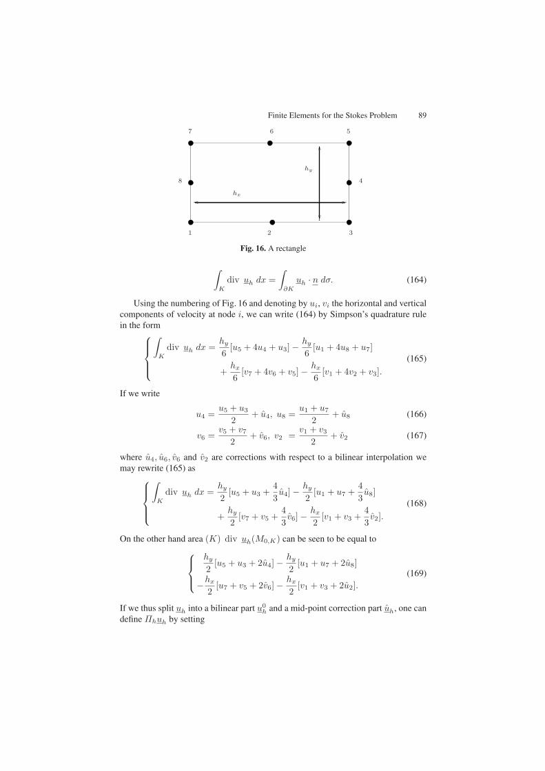
Finite Elements for the Stokes Problem 89
1 2
48
hx
hy
567
3
Fig. 16. A rectangle
∫
K
div uh dx =∫
∂K
uh · n dσ. (164)
Using the numbering of Fig. 16 and denoting by ui, vi the horizontal and verticalcomponents of velocity at node i, we can write (164) by Simpson’s quadrature rulein the form
⎧⎪⎪⎨
⎪⎪⎩
∫
K
div uh dx =hy
6[u5 + 4u4 + u3] −
hy
6[u1 + 4u8 + u7]
+hx
6[v7 + 4v6 + v5] −
hx
6[v1 + 4v2 + v3].
(165)
If we write
u4 =u5 + u3
2+ u4, u8 =
u1 + u7
2+ u8 (166)
v6 =v5 + v7
2+ v6, v2 =
v1 + v3
2+ v2 (167)
where u4, u6, v6 and v2 are corrections with respect to a bilinear interpolation wemay rewrite (165) as
⎧⎪⎪⎨
⎪⎪⎩
∫
K
div uh dx =hy
2[u5 + u3 +
43u4] −
hy
2[u1 + u7 +
43u8]
+hy
2[v7 + v5 +
43v6] −
hx
2[v1 + v3 +
43v2].
(168)
On the other hand area (K) div uh(M0,K) can be seen to be equal to⎧⎪⎨
⎪⎩
hy
2[u5 + u3 + 2u4] −
hy
2[u1 + u7 + 2u8]
−hx
2[u7 + v5 + 2v6] −
hx
2[v1 + v3 + 2u2].
(169)
If we thus split uh into a bilinear part u0h and a mid-point correction part uh, one can
define Πhuh by setting
90 D. Boffi et al.⎧⎨
⎩
(Πhuh)0 = u0h,
(Πhuh) =23uh.
(170)
Equality (164) will then hold and (170) is clearly continuous with a continuity con-stant independent of h.
Example 9.8. We come back to Example 9.4 that is a three-point quadrature rule usedin conjunction with the Crouzeix–Raviart element. We shall not give the analysis indetails but only sketch the ideas. The problem is again to check that the inf–supcondition holds through Proposition 4.1. As the quadrature rule is exact when qh ispiecewise constant, the obvious idea is to build Πhuh by keeping the trace of uh on∂K and only modifying the coefficients of the bubble functions. This can clearly bedone. Continuity is now to be checked and the proof is essentially the same as thestandard proof of the inf–sup condition (Sect. 7.2).
Example 9.9 (A modified Q1 − P0 element). We now present a puzzling exampleof an element which is stable but for which convergence is tricky due to a consis-tency error term. We have here a case where using a one-point quadrature rule willchange the situation with respect to the inf–sup condition. In fact it will make a sta-ble element from an unstable one but will also introduce an essential change in theproblem. The departure point is thus the standard Q1 − P0 element which, as weknow, does not satisfy the inf–sup condition. We now make it richer by adding to ve-locity uh|K = u1, u2 what we shall call wave functions. On the reference elementK =] − 1, 1[×] − 1, 1[, those functions are defined by
w1 = x b2(x, y),w2 = y b2(x, y),
(171)
where b2(x, y) = (1 − x2)(1 − y2) is the Q2 bubble function. If we now consider
uh|K = u1 + αKw1, u2 + αKw2 = uh|K + αKwK , (172)
we obtain a new element with an internal degree of freedom. The wave functionsthat we added vanish on the boundary and nothing is changed for the stability ofthe mixed method with exact integration. If we rather use a one-point quadraturerule, things become different. We shall indeed check that the modified bilinear formbh(vh, qh) satisfies the inf–sup condition. We thus have to show that
supu
h
∑K
div uh(M0,K)pK h2K
‖uh‖1≥ k0 |ph|0. (173)
This is easily checked by posing on K (we suppose a rectangular mesh to simplify)
uh|K = hK pKwK . (174)
We then have div uh = ph and
Finite Elements for the Stokes Problem 91
‖uh‖1,K = h pK ‖wK‖1,K , (175)
which implies‖uh‖1 ≤ c |ph|0, (176)
and (173) follows. A remarkable point is that even the hydrostatic mode has disap-peared. This is an indication that something incorrect has been introduced in the ap-proximation. An analysis of consistency error indeed shows that usual error estimatesfail and that we are actually approximating a continous problem in which the incom-pressibility condition has been replaced by div u+kp = 0 where k = 1575/416. Wethen see that if in general for Stokes problem, making the space of velocities richerimproves (at least does not reduce) the quality of the method, this fact can becomefalse when numerical integration is used.
Let us now turn our attention to the problem of error estimation. From [24] all wehave to do is to estimate the consistency terms
supvh
|bh(vh, p) − bh(vh, p)|‖vh‖V
(177)
and
supqh
|b(u, qh) − bh(u, qh)|‖qh‖0
. (178)
We thus have to estimate quadrature errors. It would be out of purpose to enter intodetails and we refer the reader to [27, 28] where examples of such analysis are pre-sented exhaustively. The first step is to transform (177) into a form which is some-times more tractable. We may indeed write
b(vh, p) − bh(vh, p) = (b(vh, p− qh) − bh(vh, p− qh))
+ (b(vh, qh) − bh(vh, qh))(179)
and b(u, qh) − bh(u, qh) = (b(u− vh, qh) − bh(u− vh, qh))
+ (b(vh, qh) − bh(vh, qh)).(180)
The first parenthesis in the right-hand side of (179) and (180) can be reduced to anapproximation error. The second parenthesis implies only polynomials.
Let us therefore consider (180) for the three approximations introduced above.(Coming back to the notations of the present section). For the Crouzeix–Raviart tri-angle taking vh the standard interpolate of u makes the second parenthesis vanishwhile the first yields an O(h) estimate. For the two other approximations taking vh
to be a standard bilinear approximation of u makes the second parenthesis vanishwhile the first yields on O(h) estimate, which is the best that we can hope any-way. The real trouble is therefore with (177) with or without (179). In the case ofthe Crouzeix–Raviart triangle, we can use directly (177) and the following resultof [27, 28], (Theorem IV.1.5).
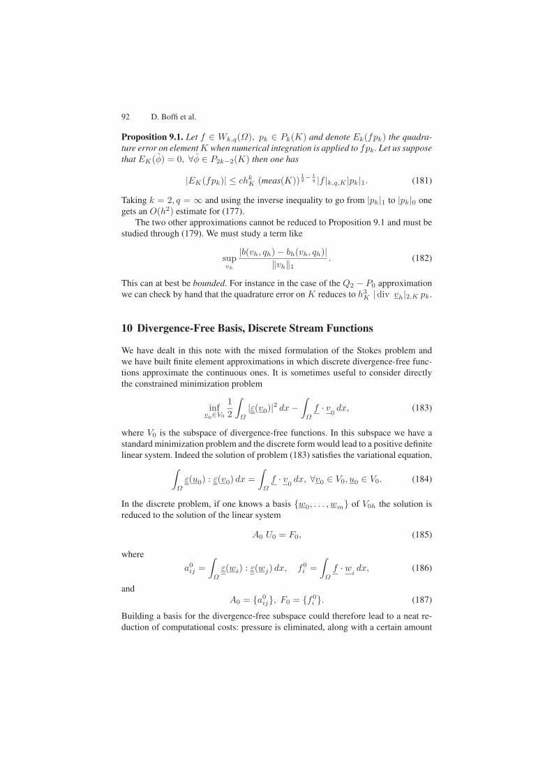
92 D. Boffi et al.
Proposition 9.1. Let f ∈ Wk,q(Ω), pk ∈ Pk(K) and denote Ek(fpk) the quadra-ture error on element K when numerical integration is applied to fpk. Let us supposethat EK(φ) = 0, ∀φ ∈ P2k−2(K) then one has
|EK(fpk)| ≤ chkK (meas(K))
12− 1
q |f |k,q,K |pk|1. (181)
Taking k = 2, q = ∞ and using the inverse inequality to go from |pk|1 to |pk|0 onegets an O(h2) estimate for (177).
The two other approximations cannot be reduced to Proposition 9.1 and must bestudied through (179). We must study a term like
supvh
|b(vh, qh) − bh(vh, qh)|‖vh‖1
. (182)
This can at best be bounded. For instance in the case of the Q2 − P0 approximationwe can check by hand that the quadrature error on K reduces to h3
K |div vh|2,K pk.
10 Divergence-Free Basis, Discrete Stream Functions
We have dealt in this note with the mixed formulation of the Stokes problem andwe have built finite element approximations in which discrete divergence-free func-tions approximate the continuous ones. It is sometimes useful to consider directlythe constrained minimization problem
infv0∈V0
12
∫
Ω
|ε(v0)|2 dx−∫
Ω
f · v0dx, (183)
where V0 is the subspace of divergence-free functions. In this subspace we have astandard minimization problem and the discrete form would lead to a positive definitelinear system. Indeed the solution of problem (183) satisfies the variational equation,
∫
Ω
ε(u0) : ε(v0) dx =∫
Ω
f · v0dx, ∀v0 ∈ V0, u0 ∈ V0. (184)
In the discrete problem, if one knows a basis w0, . . . , wm of V0h the solution isreduced to the solution of the linear system
A0 U0 = F0, (185)
wherea0
ij =∫
Ω
ε(wi) : ε(wj) dx, f0i =
∫
Ω
f · widx, (186)
andA0 = a0
ij, F0 = f0i . (187)
Building a basis for the divergence-free subspace could therefore lead to a neat re-duction of computational costs: pressure is eliminated, along with a certain amount
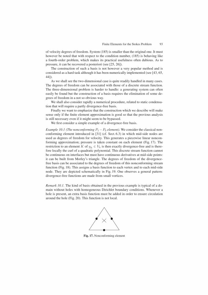
Finite Elements for the Stokes Problem 93
of velocity degrees of freedom. System (185) is smaller than the original one. It musthowever be noted that with respect to the condition number, (185) is behaving likea fourth-order problem, which makes its practical usefulness often dubious. As topressure, it can be recovered a posteriori (see [25, 26]).
The construction of such a basis is not however a very popular method and isconsidered as a hard task although it has been numerically implemented (see [43, 65,44]).
As we shall see the two-dimensional case is quite readily handled in many cases.The degrees of freedom can be associated with those of a discrete stream function.The three-dimensional problem is harder to handle: a generating system can ofteneasily be found but the construction of a basis requires the elimination of some de-grees of freedom in a not so obvious way.
We shall also consider rapidly a numerical procedure, related to static condensa-tion that will require a partly divergence-free basis.
Finally we want to emphasize that the construction which we describe will makesense only if the finite element approximation is good so that the previous analysisis still necessary even if it might seem to be bypassed.
We first consider a simple example of a divergence-free basis.
Example 10.1 (The nonconforming P1−P0 element). We consider the classical non-conforming element introduced in [31] (cf. Sect. 6.3) in which mid-side nodes areused as degrees of freedom for velocity. This generates a piecewise linear noncon-forming approximation; pressure is taken constant on each element (Fig. 17). Therestriction to an element K of uh ∈ Vh is then exactly divergence-free and is there-fore locally the curl of a quadratic polynomial. This discrete stream function cannotbe continuous on interfaces but must have continuous derivatives at mid-side points:it can be built from Morley’s triangle. The degrees of freedom of the divergence-free basis can be associated to the degrees of freedom of this nonconforming streamfunction (Fig. 18). This assigns a basis function to each vertex and to each mid-sidenode. They are depicted schematically in Fig. 19. One observes a general pattern:divergence-free functions are made from small vortices.
Remark 10.1. The kind of basis obtained in the previous example is typical of a do-main without holes with homogeneous Dirichlet boundary conditions. Whenever ahole is present, an extra basis function must be added in order to ensure circulationaround the hole (Fig. 20). This function is not local.
Fig. 17. Nonconforming element
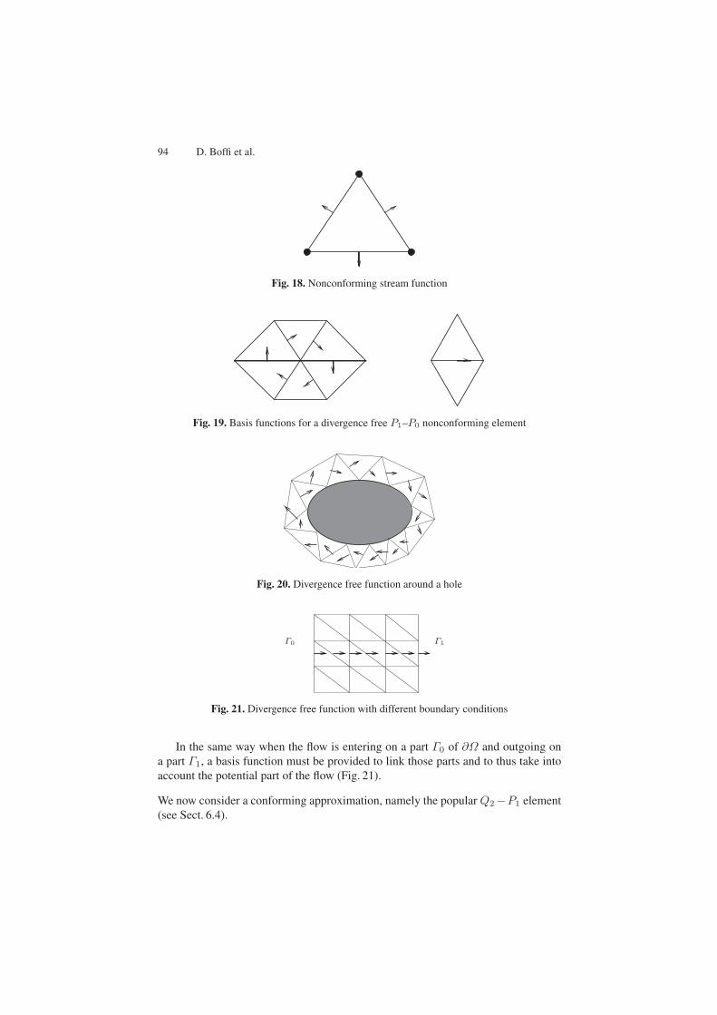
94 D. Boffi et al.
Fig. 18. Nonconforming stream function
Fig. 19. Basis functions for a divergence free P1–P0 nonconforming element
Fig. 20. Divergence free function around a hole
Γ0 Γ1
Fig. 21. Divergence free function with different boundary conditions
In the same way when the flow is entering on a part Γ0 of ∂Ω and outgoing ona part Γ1, a basis function must be provided to link those parts and to thus take intoaccount the potential part of the flow (Fig. 21).
We now consider a conforming approximation, namely the popular Q2−P1 element(see Sect. 6.4).
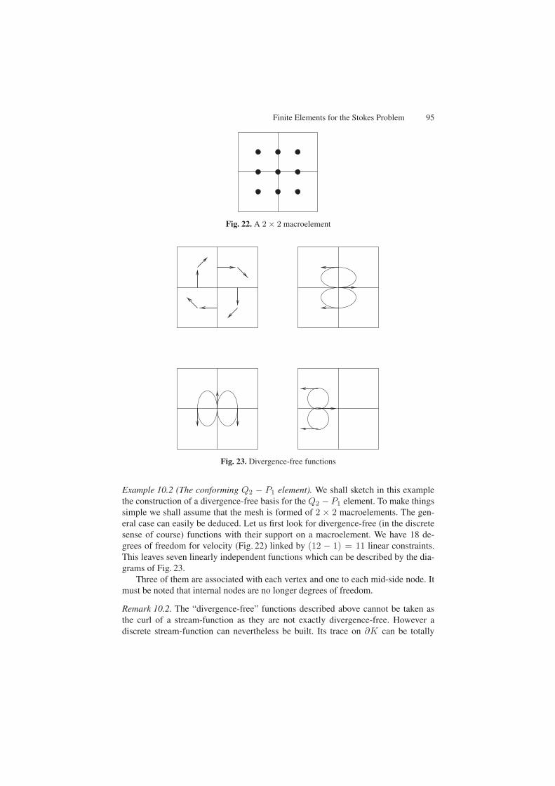
Finite Elements for the Stokes Problem 95
Fig. 22. A 2 × 2 macroelement
Fig. 23. Divergence-free functions
Example 10.2 (The conforming Q2 − P1 element). We shall sketch in this examplethe construction of a divergence-free basis for the Q2 − P1 element. To make thingssimple we shall assume that the mesh is formed of 2 × 2 macroelements. The gen-eral case can easily be deduced. Let us first look for divergence-free (in the discretesense of course) functions with their support on a macroelement. We have 18 de-grees of freedom for velocity (Fig. 22) linked by (12 − 1) = 11 linear constraints.This leaves seven linearly independent functions which can be described by the dia-grams of Fig. 23.
Three of them are associated with each vertex and one to each mid-side node. Itmust be noted that internal nodes are no longer degrees of freedom.
Remark 10.2. The “divergence-free” functions described above cannot be taken asthe curl of a stream-function as they are not exactly divergence-free. However adiscrete stream-function can nevertheless be built. Its trace on ∂K can be totally
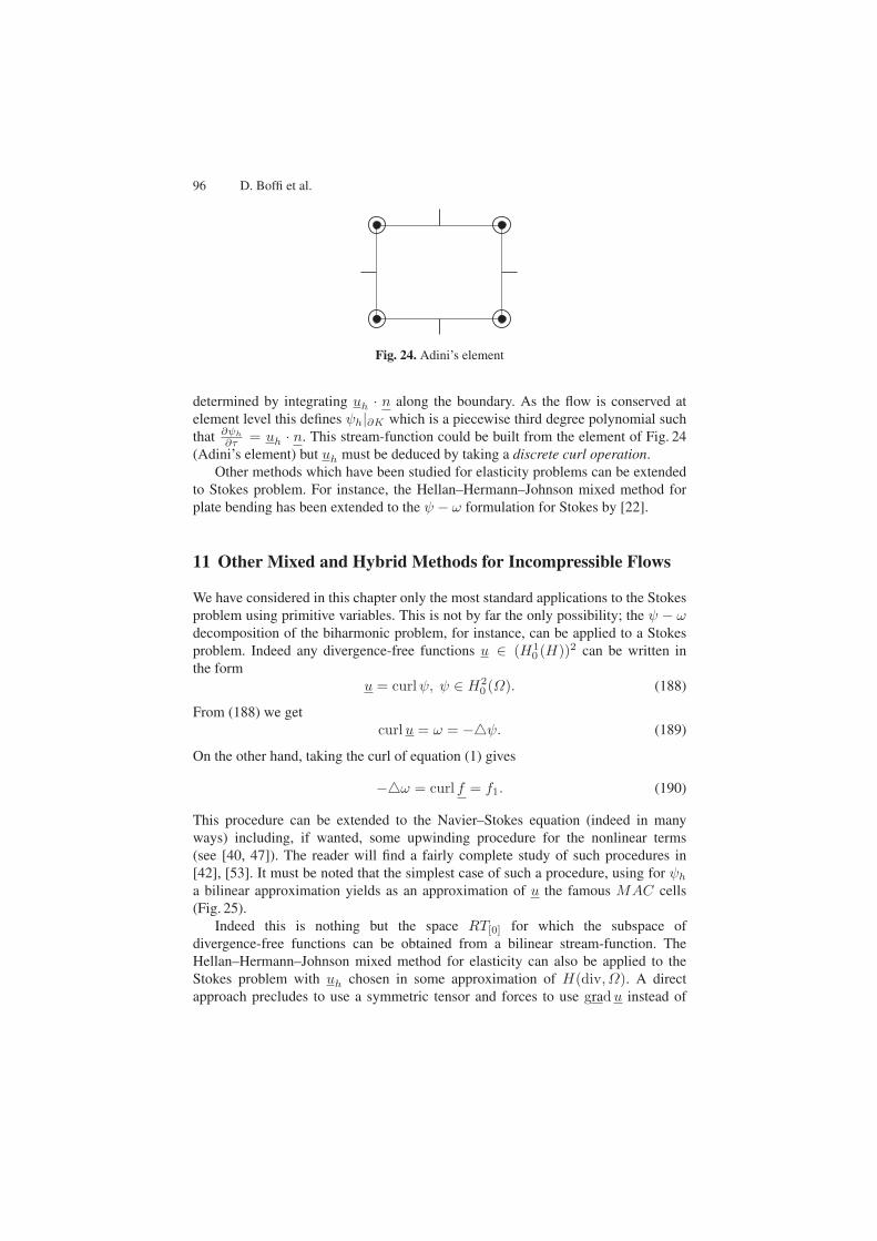
96 D. Boffi et al.
Fig. 24. Adini’s element
determined by integrating uh · n along the boundary. As the flow is conserved atelement level this defines ψh|∂K which is a piecewise third degree polynomial suchthat ∂ψh
∂τ = uh · n. This stream-function could be built from the element of Fig. 24(Adini’s element) but uh must be deduced by taking a discrete curl operation.
Other methods which have been studied for elasticity problems can be extendedto Stokes problem. For instance, the Hellan–Hermann–Johnson mixed method forplate bending has been extended to the ψ − ω formulation for Stokes by [22].
11 Other Mixed and Hybrid Methods for Incompressible Flows
We have considered in this chapter only the most standard applications to the Stokesproblem using primitive variables. This is not by far the only possibility; the ψ − ωdecomposition of the biharmonic problem, for instance, can be applied to a Stokesproblem. Indeed any divergence-free functions u ∈ (H1
0 (H))2 can be written inthe form
u = curlψ, ψ ∈ H20 (Ω). (188)
From (188) we getcurlu = ω = −ψ. (189)
On the other hand, taking the curl of equation (1) gives
−ω = curl f = f1. (190)
This procedure can be extended to the Navier–Stokes equation (indeed in manyways) including, if wanted, some upwinding procedure for the nonlinear terms(see [40, 47]). The reader will find a fairly complete study of such procedures in[42], [53]. It must be noted that the simplest case of such a procedure, using for ψh
a bilinear approximation yields as an approximation of u the famous MAC cells(Fig. 25).
Indeed this is nothing but the space RT[0] for which the subspace ofdivergence-free functions can be obtained from a bilinear stream-function. TheHellan–Hermann–Johnson mixed method for elasticity can also be applied to theStokes problem with uh chosen in some approximation of H(div, Ω). A directapproach precludes to use a symmetric tensor and forces to use gradu instead of
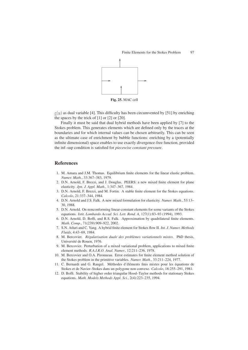
Finite Elements for the Stokes Problem 97
Fig. 25. MAC cell
ε(u) as dual variable [4]. This difficulty has been circumvented by [51] by enrichingthe spaces by the trick of [1] or [2] or [20].
Finally it must be said that dual hybrid methods have been applied by [7] to theStokes problem. This generates elements which are defined only by the traces at theboundaries and for which internal values can be chosen arbitrarily. This can be seenas the ultimate case of enrichment by bubble functions: enriching by a (potentiallyinfinite dimensional) space enables to use exactly divergence-free function, providedthe inf–sup condition is satisfied for piecewise constant pressure.
References
1. M. Amara and J.M. Thomas. Equilibrium finite elements for the linear elastic problem.Numer. Math., 33:367–383, 1979.
2. D.N. Arnold, F. Brezzi, and J. Douglas. PEERS: a new mixed finite element for planeelasticity. Jpn. J. Appl. Math., 1:347–367, 1984.
3. D.N. Arnold, F. Brezzi, and M. Fortin. A stable finite element for the Stokes equations.Calcolo, 21:337–344, 1984.
4. D.N. Arnold and J.S. Falk. A new mixed formulation for elasticity. Numer. Math., 53:13–30, 1988.
5. D.N. Arnold. On nonconforming linear-constant elements for some variants of the Stokesequations. Istit. Lombardo Accad. Sci. Lett. Rend. A, 127(1):83–93 (1994), 1993.
6. D.N. Arnold, D. Boffi, and R.S. Falk. Approximation by quadrilateral finite elements.Math. Comp., 71(239):909–922, 2002.
7. S.N. Atluri and C. Yang. A hybrid finite element for Stokes flow II. Int. J. Numer. MethodsFluids, 4:43–69, 1984.
8. M. Bercovier. Regularisation duale des problemes variationnels mixtes. PhD thesis,Universite de Rouen, 1976.
9. M. Bercovier. Perturbation of a mixed variational problem, applications to mixed finiteelement methods. R.A.I.R.O. Anal. Numer., 12:211–236, 1978.
10. M. Bercovier and O.A. Pironneau. Error estimates for finite element method solution ofthe Stokes problem in the primitive variables. Numer. Math., 33:211–224, 1977.
11. C. Bernardi and G. Raugel. Methodes d’elements finis mixtes pour les equations deStokes et de Navier–Stokes dans un polygone non convexe. Calcolo, 18:255–291, 1981.
12. D. Boffi. Stability of higher order triangular Hood–Taylor methods for stationary Stokesequations. Math. Models Methods Appl. Sci., 2(4):223–235, 1994.
98 D. Boffi et al.
13. D. Boffi. Minimal stabilizations of the Pk+1−Pk approximation of the stationary Stokesequations. Math. Models Methods Appl. Sci., 5(2):213–224, 1995.
14. D. Boffi. Three-dimensional finite element methods for the Stokes problem. SIAM J.Numer. Anal., 34:664–670, 1997.
15. D. Boffi and L. Gastaldi. On the quadrilateral Q2 − P1 element for the Stokes problem.Int. J. Numer. Methods Fluids, 39:1001–1011, 2002.
16. D. Boffi and C. Lovadina. Analysis of new augmented Lagrangian formulations for mixedfinite element schemes. Numer. Math., 75(4):405–419, 1997.
17. D. Boffi, F. Brezzi, and L. Gastaldi. On the problem of spurious eigenvalues in the ap-proximation of linear elliptic problems in mixed form. Math. Comput., 69(229):121–140,2000.
18. J.M. Boland and R.A. Nicolaides. Stability of finite elements under divergence con-straints. SIAM J. Numer. Anal., 20(4):722–731, 1983.
19. F. Brezzi and K.J. Bathe. A discourse on the stability conditions for mixed finite elementformulations. CMAME, 82:27–57, 1990.
20. F. Brezzi, J. Douglas, Jr., and L.D. Marini. Recent results on mixed finite element methodsfor second order elliptic problems. Vistas in applied mathematics, 25–43, Transl. Ser.Math. Engrg., Optimization Software, New York, 1986.
21. F. Brezzi and R.S. Falk. Stability of higher-order Hood-Taylor methods. SIAM J. Numer.Anal., 28(3):581–590, 1991.
22. F. Brezzi, J. Le Tellier, and T. Olier. Mixed finite element approximation for the stationaryNavier–Stokes equations (in Russian). In Viceslitelnia Metodii V. Prikladnoi Mathemat-iceskie, NAUKA, Novosibirsk, 1982, pp. 96–108. Meeting INRIA, Novosibirsk.
23. F. Brezzi and J. Pitkaranta. On the stabilization of finite element approximations of theStokes equations. In W. Hackbush, editor, Efficient Solutions of Elliptic Systems, Noteson Numerical Fluid Mechanics, vol. 10, Braunschweig, Wiesbaden, Vieweg, 1984.
24. F. Brezzi and M. Fortin. Mixed and Hybrid Finite Element Methods. Springer, BerlinHeidelberg New York, 1991.
25. P. Caussignac. Explicit basis functions of quadratic and improved quadratic finite elementspaces for the Stokes problem. Commun. Appl. Numer. Methods, 2:205–211, 1986.
26. P. Caussignac. Computation of pressure from the finite element vorticity stream-functionapproximation of the Stokes problem. Commum. Appl. Numer. Methods, 3:287–295,1987.
27. P.G. Ciarlet. Mathematical elasticity, vol. I. Three-Dimensional Elasticity. North-Holland, Amsterdam, 1988.
28. P.G. Ciarlet. Mathematical elasticity, vol. II. Theory of Plates. North-Holland,Amsterdam, 1997.
29. J.F. Ciavaldini and J.C. Nedelec. Sur l’element de Fraeijs de Veubeke et Sander.R.A.I.R.O. Anal. Numer., 8:29–45, 1974.
30. P. Clement. Approximation by finite element functions using local regularization.R.A.I.R.O. Anal. Numer., 9:77–84, 1975.
31. M. Crouzeix and P.A. Raviart. Conforming and nonconforming finite element methodsfor solving the stationary Stokes equations. R.A.I.R.O. Anal. Numer., 7:33–76, 1973.
32. G. Duvaut and J.L. Lions. Les inequations en mecanique et en physique. Dunod, Paris,1972.
33. A. Fortin. Methodes d’elements finis pour les equations de Navier–Stokes. PhD thesis,Universite Laval, 1984.
Finite Elements for the Stokes Problem 99
34. A. Fortin and M. Fortin. Newer and newer elements for incompressible flow. InR.H. Gallagher, G.F. Carey, J.T. Oden, and O.C. Zienkiewicz, editors, Finite Elementsin Fluids, Volume 6. Chichester, England and New York, Wiley-Interscience, 1985,p. 171–187.
35. M. Fortin. Utilisation de la methode des elements finis en mecanique des fluides. Calcolo,12:405–441, 1975.
36. M. Fortin. An analysis of the convergence of mixed finite element methods. R.A.I.R.O.Anal. Numer., 11:341–354, 1977.
37. M. Fortin. Old and new finite elements for incompressible flows. Int. J. Numer. MethodsFluids, 1:347–364, 1981.
38. M. Fortin, R. Peyret, and R. Temam. Resolution numerique des equations de Navier–Stokes pour un fluide visqueux incompressible. J. Mecanique, 10, 3:357–390, 1971.
39. M. Fortin and M. Soulie. A nonconforming piecewise quadratic finite element on trian-gles. Int. J. Numer. Methods Eng., 19:505–520, 1983.
40. M. Fortin and F. Thomasset. Mixed finite element methods for incompressible flow prob-lems. J. Comput. Physics, 37:173–215, 1979.
41. V. Girault and P.A. Raviart. Finite Element Methods for Navier–Stokes Equations, Theoryand Algorithms. Springer, Berlin Heidelberg New York, 1986.
42. R. Glowinski and O. Pironneau. Numerical methods for the first biharmonic equation andfor the two-dimensional Stokes problem. SIAM Rev., 17:167–212, 1979.
43. D. Griffiths. Finite elements for incompressible flow. Math. Methods Appl. Sci., 1:16–31,1979.
44. F. Hecht. Construction d’une base de fontions P1 non-conformes a divergence nulle dansR
3. R.A.I.R.O. Anal. Numer., 15:119–150, 1981.45. P. Hood and C. Taylor. Numerical solution of the Navier–Stokes equations using the finite
element technique. Comput. Fluids, 1:1–28, 1973.46. T.J.R. Hughes and H. Allik. Finite elements for compressible and incompressible con-
tinua. In Proceedings of the Symposium on Civil Engineering, Nashville, TN. VanderbiltUniversity, 1969, pp. 27–62.
47. C. Johnson. On the convergence of a mixed finite element method for plate bendingproblems. Numer. Math., 21:43–62, 1973.
48. C. Johnson and J. Pitkaranta. Analysis of some mixed finite element methods related toreduced integration. Math. Comput., 38:375–400, 1982.
49. D.S. Malkus. Eigenproblems associated with the discrete LBB-condition for incompress-ible finite elements. Int. J. Eng. Sci., 19:1299–1310, 1981.
50. D.S Malkus and T.J.R. Hughes. Mixed finite element methods. reduced and selectiveintegration techniques: a unification of concepts. Comput. Methods Appl. Mech. Eng.,15:63–81, 1978.
51. Z. Mghazli. Une methode mixte pour les equations de l’hydrodynamique. PhD thesis,Universite de Montreal, 1987.
52. J.T. Oden and O. Jacquotte. Stability of some mixed finite element methods for Stokesianflows. Comput. Methods Appl. Mech. Eng., 43:231–247, 1984.
53. O. Pironneau. Finite Element Methods for Fluids. John Wiley, Chichester, 1989. Trans-lated from the French.
54. J. Qin. On the convergence of some simple finite elements for incompressible flows. PhDthesis, Penn State University, 1994.
55. R. Rannacher and S. Turek. Simple nonconforming quadrilateral Stokes element. Numer.Methods Partial Differ. Equations, 8(2):97–111, 1992.
100 D. Boffi et al.
56. R.L. Sani, P.M. Gresho, R.L. Lee, and D.F. Griffiths. The cause and cure (?) of thespurious pressures generated by certain FEM solutions of the incompressible Navier–Stokes equations. I. Int. J. Numer. Methods Fluids, 1(1):17–43, 1981.
57. R. L. Sani, P. M. Gresho, R. L. Lee, D. F. Griffiths, and M. Engelman. The cause and cure(!) of the spurious pressures generated by certain FEM solutions of the incompressibleNavier–Stokes equations. II. Int. J. Numer. Methods Fluids, 1(2):171–204, 1981.
58. L.R. Scott and M. Vogelius. Norm estimates for a maximal right inverse of the divergenceoperator in spaces of piecewise polynomials. Math. Model. Numer. Anal., 9:11–43, 1985.
59. R. Stenberg. Analysis of mixed finite element methods for the Stokes problem: a unifiedapproach. Math. Comput., 42:9–23, 1984.
60. R. Stenberg. On the construction of optimal mixed finite element methods for the linearelasticity problem. Numer. Math., 48:447–462, 1986.
61. R. Stenberg. On some three-dimensional finite elements for incompressible media. Com-put. Methods Appl. Mech. Eng., 63:261–269, 1987.
62. R. Stenberg. On the postprocessing of mixed equilibrium finite element methods. InW. Hackbusch and K. Witsch, editors, Numerical Tehchniques in Continuum Mechanics.Veiweg, Braunschweig, 1987. Proceedings of the Second GAMM-Seminar, Kiel, 1986.
63. R. Stenberg. Error analysis of some finite element methods for the Stokes problem. Math.Comput., 54(190):495–508, 1990. Chesnay, France, 1988.
64. R. Temam. Navier–Stokes Equations. North-Holland, Amsterdam, 1977.65. F. Thomasset. Implementation of Finite Element Methods for Navier–Stokes Equations.
Springer Series in Computational Physics. Springer, Berlin Heidelberg New York, 1981.66. R. Verfurth. Error estimates for a mixed finite element approximation of the Stokes equa-
tion. R.A.I.R.O. Anal. Numer., 18:175–182, 1984.67. O.C. Zienkiewicz, S. Qu, R.L. Taylor, and S. Nakazawa. The patch text for mixed formu-
lations. Int. J. Numer. Methods Eng., 23:1873–1883, 1986.