Mixed Designs:

Between and Within

Psy 420

Ainsworth

Mixed Between and Within Designs

• Conceptualizing the Design

▫ Types of Mixed Designs

• Assumptions

• Analysis

▫ Deviation

▫ Computation

• Higher order mixed designs

• Breaking down significant effects

Conceptualizing the Design

• This is a very popular design because you are combining the benefits of each design

• Requires that you have one between groups IV and one within subjects IV

• Often called “Split-plot” designs, which comes from agriculture

• In the simplest 2 x 2 design you would have

Conceptualizing the Design

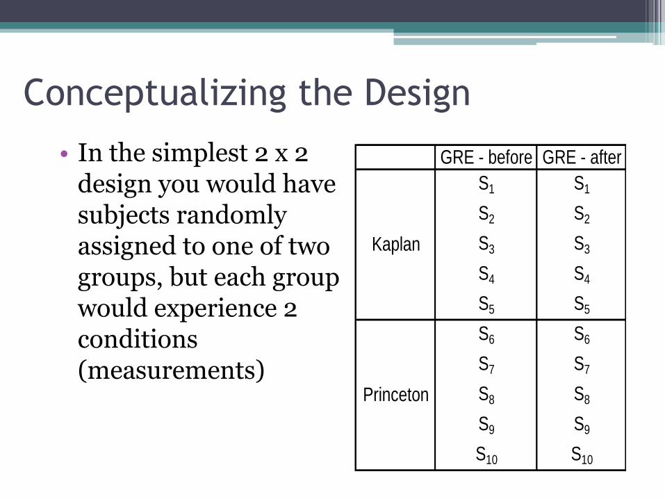
• In the simplest 2 x 2 design you would have subjects randomly assigned to one of two groups, but each group would experience 2 conditions (measurements)

GRE - before GRE - after

S1 S1

S2 S2

S3 S3

S4 S4

S5 S5

S6 S6

S7 S7

S8 S8

S9 S9

S10 S10

Kaplan

Princeton

Conceptualizing the Design

• Advantages

▫ First, it allows generalization of the repeated measures over the randomized groups levels

▫ Second, reduced error (although not as reduced as purely WS) due to the use of repeated measures

• Disadvantages

▫ The addition of each of their respective complexities

Conceptualizing the Design

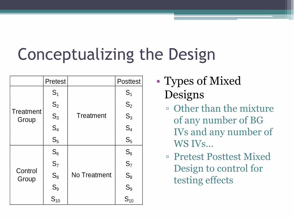
Pretest Posttest

S1 S1

S2 S2

S3 S3

S4 S4

Treatment Group

S5

Treatment

S5

S6 S6

S7 S7

S8 S8

S9 S9

Control Group

S10

No Treatment

S10

• Types of Mixed Designs▫ Other than the mixture

of any number of BG IVs and any number of WS IVs…

▫ Pretest Posttest Mixed Design to control for testing effects

Assumptions

• Normality of Sampling Distribution of the BG IVs

▫ Applies to the case averages (averaged over the WS levels)

• Homogeneity of Variance

▫ Applies to every level or combination of levels of the BG IV(s)

Assumptions

• Independence, Additivity, Sphericity

▫ Independence applies to the BG error term

▫ But each WS error term confounds random variability with the subjects by effects interaction

▫ So we need to test for sphericity instead; the test is on the average variance/covariance matrix (over the levels of the BG IVs)

Assumptions

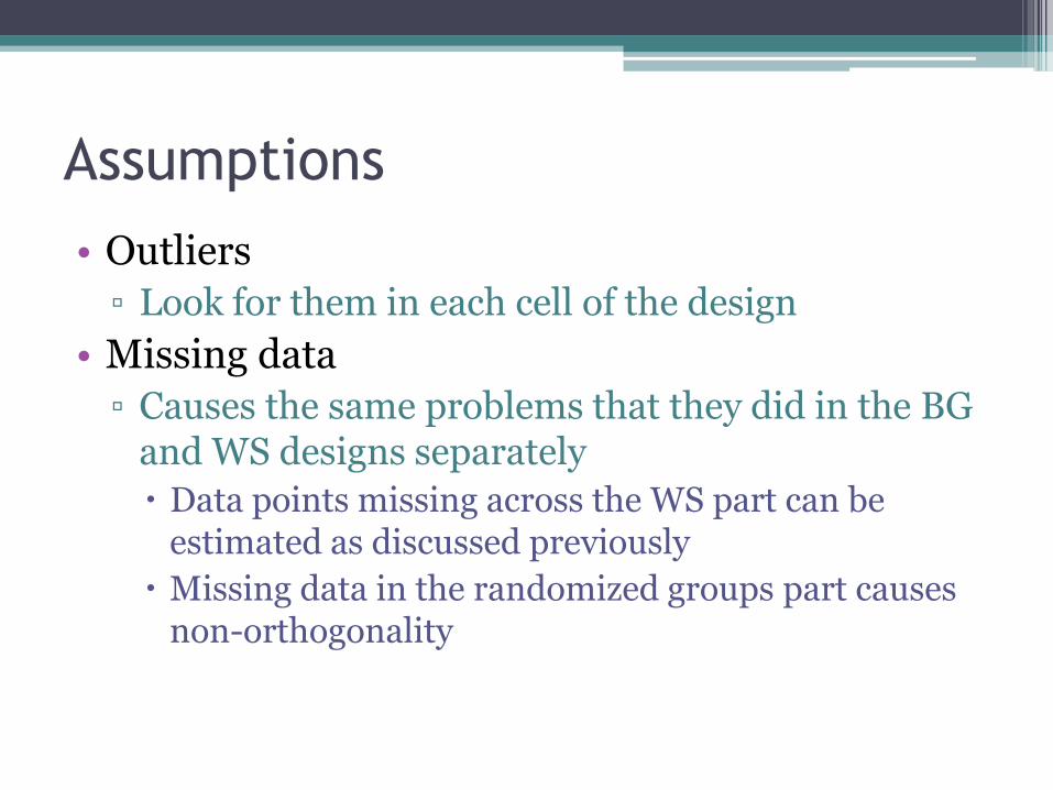
• Outliers

▫ Look for them in each cell of the design

• Missing data

▫ Causes the same problems that they did in the BG and WS designs separately

Data points missing across the WS part can be estimated as discussed previously

Missing data in the randomized groups part causes non-orthogonality

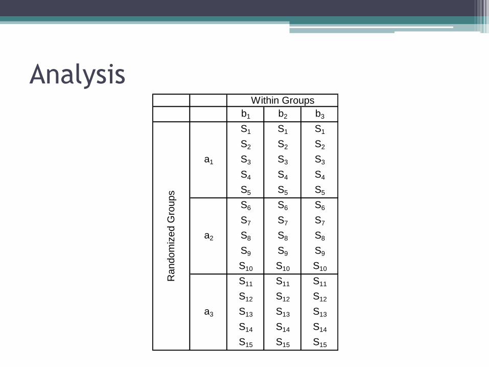
Analysis

b1 b2 b3

S1 S1 S1

S2 S2 S2

S3 S3 S3

S4 S4 S4

S5 S5 S5

S6 S6 S6

S7 S7 S7

S8 S8 S8

S9 S9 S9

S10 S10 S10

S11 S11 S11

S12 S12 S12

S13 S13 S13

S14 S14 S14

S15 S15 S15

Within Groups

a1

a2

a3

Ra

ndo

miz

ed G

roup

s

Sources of Variance

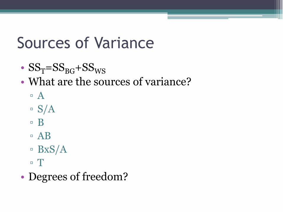
• SST=SSBG+SSWS

• What are the sources of variance?

▫ A

▫ S/A

▫ B

▫ AB

▫ BxS/A

▫ T

• Degrees of freedom?

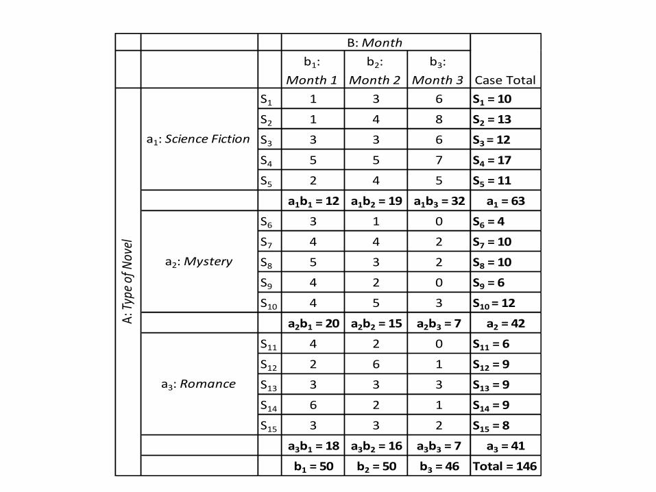
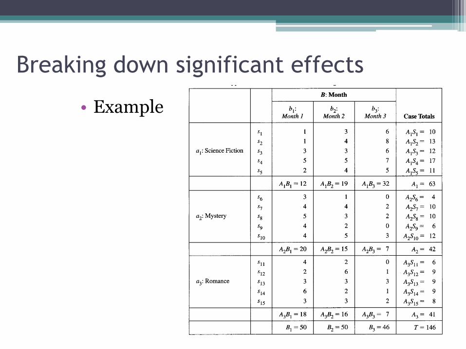
Example – Books by Month

• Example:

▫ Imagine if we designed the previous research study concerning reading different novels over time

▫ But instead of having everyone read all of the books for three months we randomly assign subjects to three different books and have them read for three months

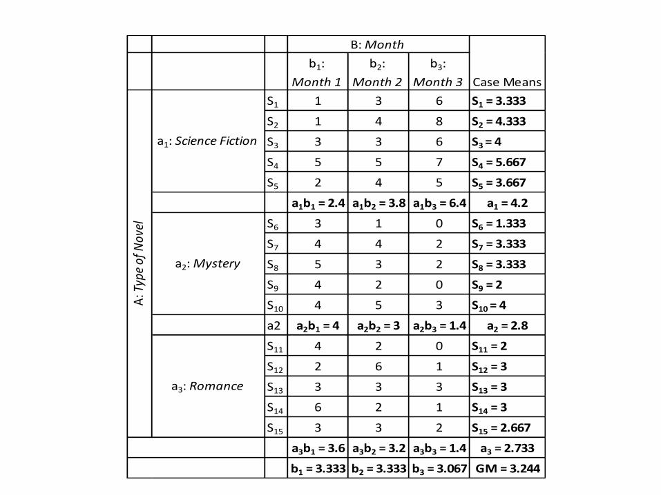
b1:

Month 1

b2:

Month 2

b3:

Month 3

S1 1 3 6 S1 = 3.333

S2 1 4 8 S2 = 4.333

S3 3 3 6 S3 = 4

S4 5 5 7 S4 = 5.667

S5 2 4 5 S5 = 3.667

a1b1 = 2.4 a1b2 = 3.8 a1b3 = 6.4 a1 = 4.2

S6 3 1 0 S6 = 1.333

S7 4 4 2 S7 = 3.333

S8 5 3 2 S8 = 3.333

S9 4 2 0 S9 = 2

S10 4 5 3 S10 = 4

a2 a2b1 = 4 a2b2 = 3 a2b3 = 1.4 a2 = 2.8

S11 4 2 0 S11 = 2

S12 2 6 1 S12 = 3

S13 3 3 3 S13 = 3

S14 6 2 1 S14 = 3

S15 3 3 2 S15 = 2.667

a3b1 = 3.6 a3b2 = 3.2 a3b3 = 1.4 a3 = 2.733

b1 = 3.333 b2 = 3.333 b3 = 3.067 GM = 3.244

B: Month

A: T

ype

of N

ovel

Case Means

a1: Science Fiction

a2: Mystery

a3: Romance

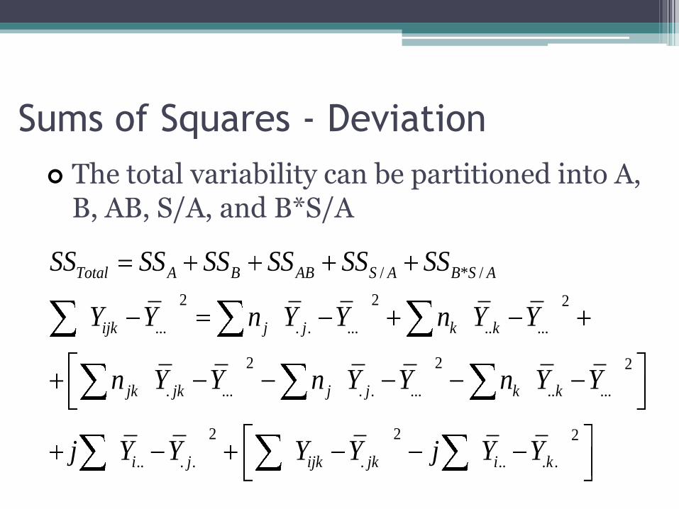
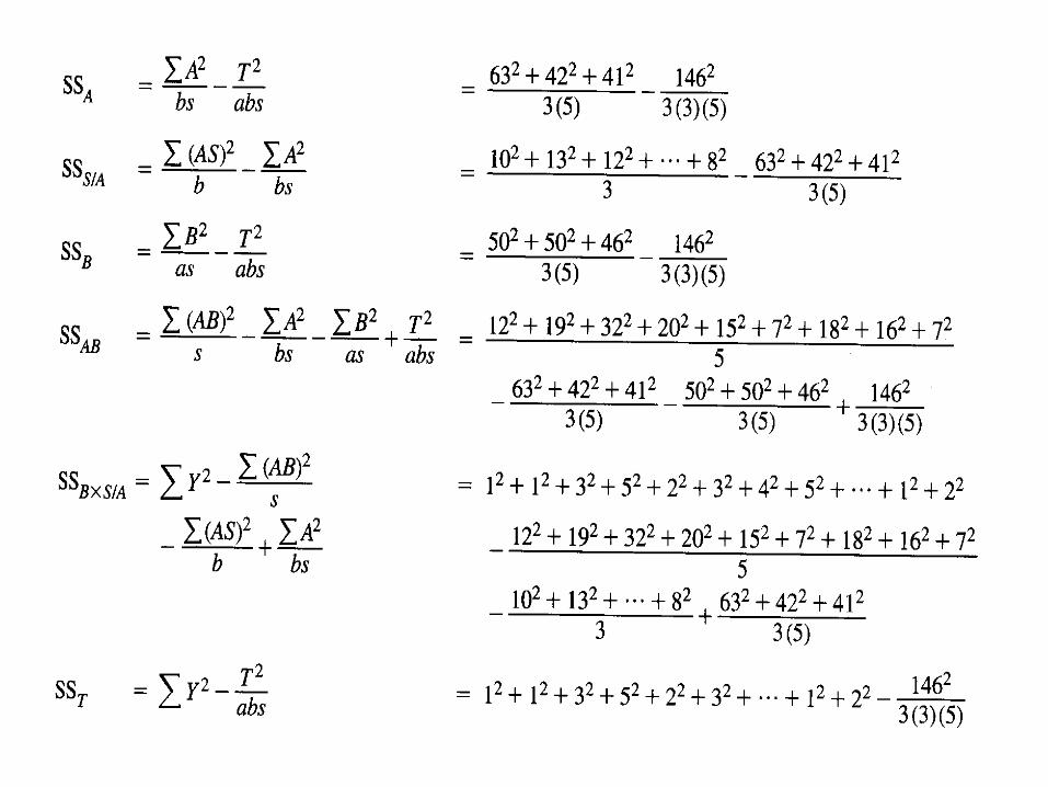
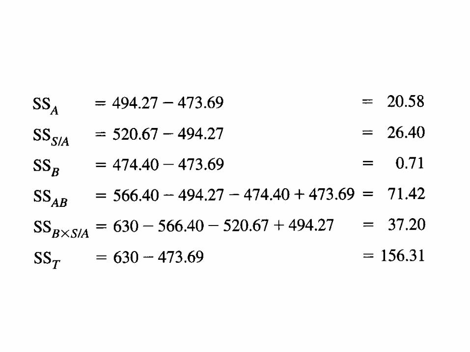
Sums of Squares - Deviation

/ * /

2 2 2

... . . ... .. ...

2 2 2

. ... . . ... .. ...

2 2 2

.. . . . .. . .

Total A B AB S A B S A

ijk j j k k

jk jk j j k k

i j ijk jk i k

SS SS SS SS SS SS

Y Y n Y Y n Y Y

n Y Y n Y Y n Y Y

j Y Y Y Y j Y Y

The total variability can be partitioned into A, B, AB, S/A, and B*S/A

2 2 2 2

. . ...

2 2 2 2

.. ...

2 2 2

. ... . . ... .. ...

2

. ...

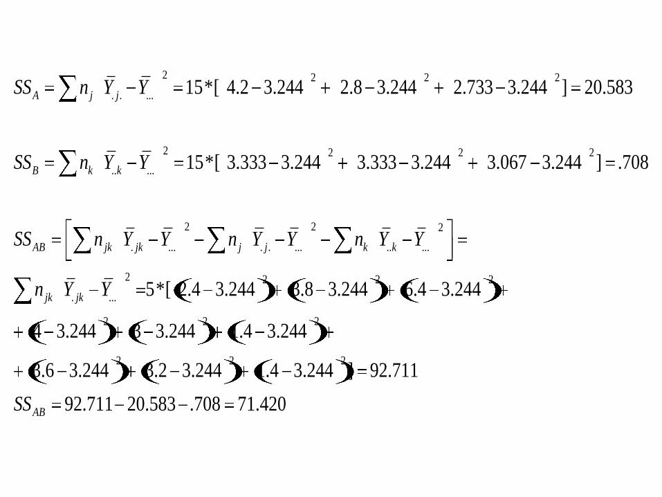
15*[ 4.2 3.244 2.8 3.244 2.733 3.244 ] 20.583

15*[ 3.333 3.244 3.333 3.244 3.067 3.244 ] .708

5

A j j

B k k

AB jk jk j j k k

jk jk

SS n Y Y

SS n Y Y

SS n Y Y n Y Y n Y Y

n Y Y2 2 2

2 2 2

2 2 2

*[ 2.4 3.244 3.8 3.244 6.4 3.244

4 3.244 3 3.244 1.4 3.244

3.6 3.244 3.2 3.244 1.4 3.244 ] 92.711

92.711 20.583 .708 71.420ABSS

2 2 2 2

/ .. . .

2 2 2 2 2

2 2 2 2 2

2 2

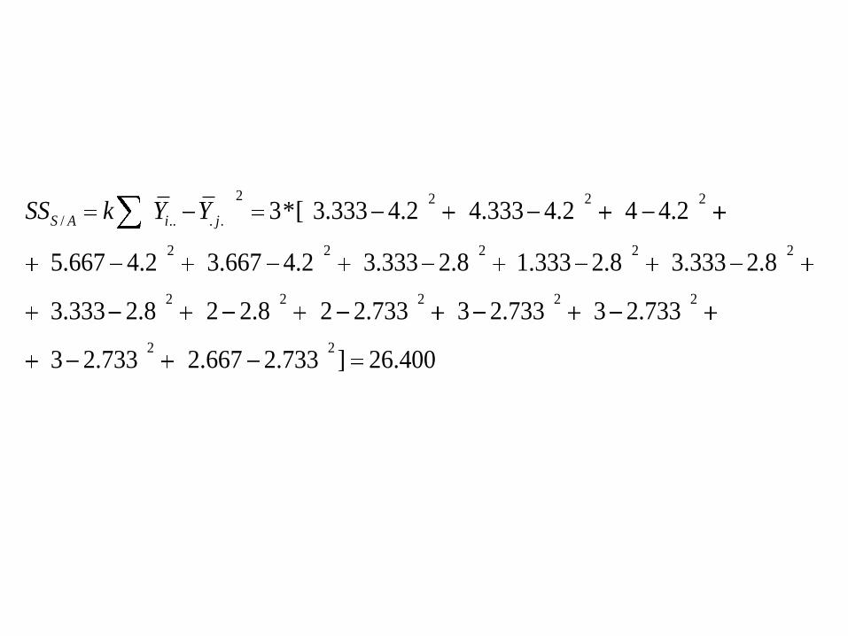
3*[ 3.333 4.2 4.333 4.2 4 4.2

5.667 4.2 3.667 4.2 3.333 2.8 1.333 2.8 3.333 2.8

3.333 2.8 2 2.8 2 2.733 3 2.733 3 2.733

3 2.733 2.667 2.733 ] 26.400

S A i jSS k Y Y

2 2

* / . .. . .

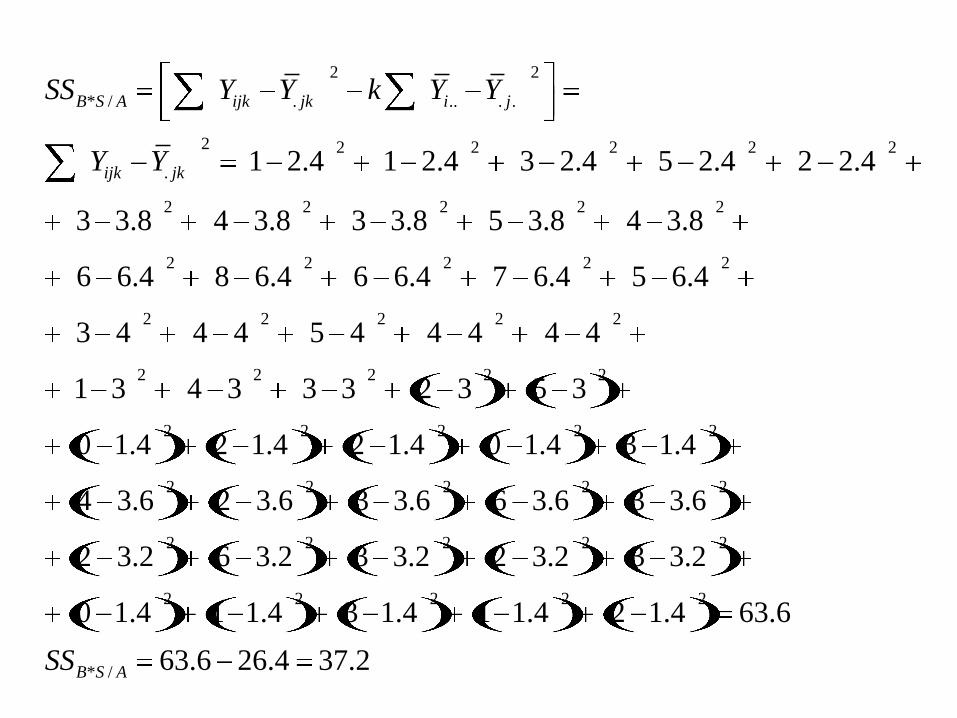
2 2 2 2 2 2

.

2 2 2 2 2

2 2 2 2 2

2 2 2 2 2

2 2 2

1 2.4 1 2.4 3 2.4 5 2.4 2 2.4

3 3.8 4 3.8 3 3.8 5 3.8 4 3.8

6 6.4 8 6.4 6 6.4 7 6.4 5 6.4

3 4 4 4 5 4 4 4 4 4

1 3 4 3 3 3

B S A ijk jk i j

ijk jk

SS Y Y k Y Y

Y Y

2 2

2 2 2 2 2

2 2 2 2 2

2 2 2 2 2

2 2 2 2 2

* /

2 3 5 3

0 1.4 2 1.4 2 1.4 0 1.4 3 1.4

4 3.6 2 3.6 3 3.6 6 3.6 3 3.6

2 3.2 6 3.2 3 3.2 2 3.2 3 3.2

0 1.4 1 1.4 3 1.4 1 1.4 2 1.4 63.6

63.6 26.4 37.2B S ASS

2

...

2 2 2 2 2

2 2 2 2 2

2 2 2 2 2

2 2 2

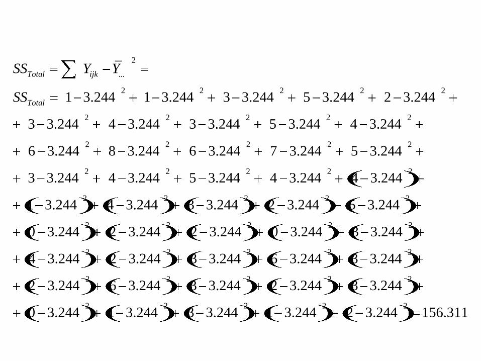
1 3.244 1 3.244 3 3.244 5 3.244 2 3.244

3 3.244 4 3.244 3 3.244 5 3.244 4 3.244

6 3.244 8 3.244 6 3.244 7 3.244 5 3.244

3 3.244 4 3.244 5 3.244 4 3.244

Total ijk

Total

SS Y Y

SS

2 2

2 2 2 2 2

2 2 2 2 2

2 2 2 2 2

2 2 2 2 2

4 3.244

1 3.244 4 3.244 3 3.244 2 3.244 5 3.244

0 3.244 2 3.244 2 3.244 0 3.244 3 3.244

4 3.244 2 3.244 3 3.244 6 3.244 3 3.244

2 3.244 6 3.244 3 3.244 2 3.244 3 3.244

0 3.2 2 2 2 2

244 1 3.244 3 3.244 1 3.244 2 3.244 156.311

b1:

Month 1

b2:

Month 2

b3:

Month 3

S1 1 3 6 S1 = 10

S2 1 4 8 S2 = 13

S3 3 3 6 S3 = 12

S4 5 5 7 S4 = 17

S5 2 4 5 S5 = 11

a1b1 = 12 a1b2 = 19 a1b3 = 32 a1 = 63

S6 3 1 0 S6 = 4

S7 4 4 2 S7 = 10

S8 5 3 2 S8 = 10

S9 4 2 0 S9 = 6

S10 4 5 3 S10 = 12

a2b1 = 20 a2b2 = 15 a2b3 = 7 a2 = 42

S11 4 2 0 S11 = 6

S12 2 6 1 S12 = 9

S13 3 3 3 S13 = 9

S14 6 2 1 S14 = 9

S15 3 3 2 S15 = 8

a3b1 = 18 a3b2 = 16 a3b3 = 7 a3 = 41

b1 = 50 b2 = 50 b3 = 46 Total = 146

B: Month

Case Total

A: T

ype

of N

ovel

a1: Science Fiction

a2: Mystery

a3: Romance

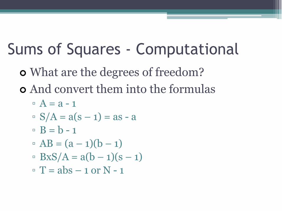
Sums of Squares - Computational

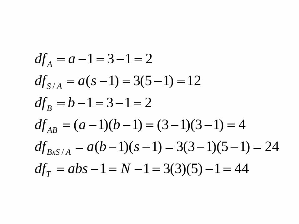
What are the degrees of freedom?

And convert them into the formulas▫ A = a - 1

▫ S/A = a(s – 1) = as - a

▫ B = b - 1

▫ AB = (a – 1)(b – 1)

▫ BxS/A = a(b – 1)(s – 1)

▫ T = abs – 1 or N - 1

/

/

1 3 1 2

( 1) 3(5 1) 12

1 3 1 2

( 1)( 1) (3 1)(3 1) 4

( 1)( 1) 3(3 1)(5 1) 24

1 1 3(3)(5) 1 44

A

S A

B

AB

BxS A

T

df a

df a s

df b

df a b

df a b s

df abs N

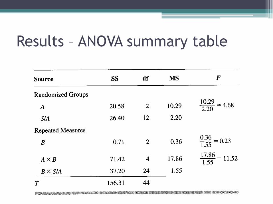
Results – ANOVA summary table

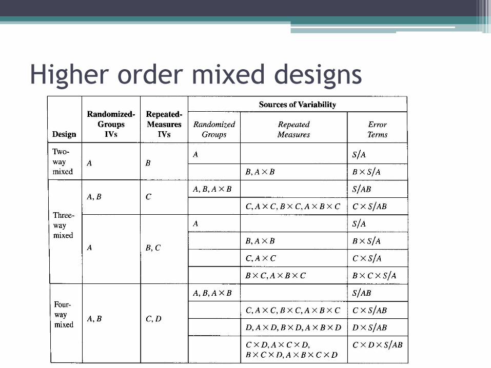
Higher order mixed designs

Breaking down significant effects

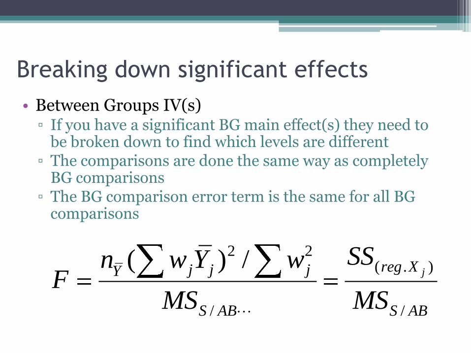
• Between Groups IV(s)▫ If you have a significant BG main effect(s) they need to

be broken down to find which levels are different▫ The comparisons are done the same way as completely

BG comparisons▫ The BG comparison error term is the same for all BG

comparisons

2 2( . )

/ /

( ) /jreg Xj j jY

S AB S AB

SSn w Y wF

MS MS

Breaking down significant effects

• Within Groups Variables

▫ If a WG main effect is significant it also needs to be followed by comparisons

▫ WG comparisons differ from BG variables in that a separate error term needs to be generated for each comparison

▫ Instead of the Fcomp formula you would actually rearrange the data into a new data set

Breaking down significant effects

• Example

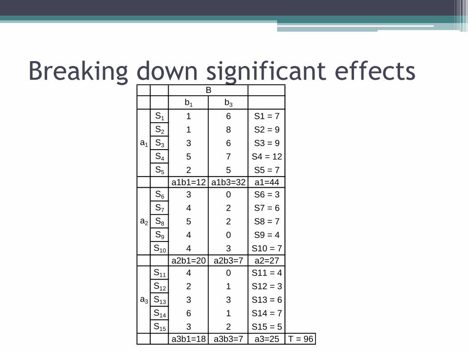
Breaking down significant effectsb1 b3

S1 1 6 S1 = 7

S2 1 8 S2 = 9

S3 3 6 S3 = 9

S4 5 7 S4 = 12

S5 2 5 S5 = 7

a1b1=12 a1b3=32 a1=44

S6 3 0 S6 = 3

S7 4 2 S7 = 6

S8 5 2 S8 = 7

S9 4 0 S9 = 4

S10 4 3 S10 = 7

a2b1=20 a2b3=7 a2=27

S11 4 0 S11 = 4

S12 2 1 S12 = 3

S13 3 3 S13 = 6

S14 6 1 S14 = 7

S15 3 2 S15 = 5

a3b1=18 a3b3=7 a3=25 T = 96

a1

a2

a3

B

Breaking down significant effects

• Interactions

▫ Purely BG interactions can be treated with simple effects, simple contrasts and interaction contrasts using the Fcomp formula, the same error term each time

▫ Purely WG and mixed BG/WG interactions require a new error term for each simple effect, simple contrast and interaction contrast (leave it to SPSS)