MIT OpenCourseWare · MIT OpenCourseWare Solutions Manual for Electromechanical Dynamics For any...

MIT OpenCourseWare http://ocw.mit.edu Solutions Manual for Electromechanical Dynamics For any use or distribution of this solutions manual, please cite as follows: Woodson, Herbert H., James R. Melcher. Solutions Manual for Electromechanical Dynamics. vols. 1 and 2. (Massachusetts Institute of Technology: MIT OpenCourseWare). http://ocw.mit.edu (accessed MM DD, YYYY). License: Creative Commons Attribution-NonCommercial-Share Alike For more information about citing these materials or our Terms of Use, visit: http://ocw.mit.edu/terms

http://ocw.mit.edu

http://ocw.mit.edu/

http://ocw.mit.edu/terms

LUMPED-PARAMETER ELECTROMECHANICAL DYNAMICS

PROBLEM 5.1

Part a

The capacitance of the system of plane parallel electrodes is

C = (L+x)dEo/s (a)

1 2 and since the co-energy W' of an electrically linear system is simply -CCv

(remember v is the terminal voltage of the capacitor, not the voltage of the

driving source)

fe 9W' I dEo 2- --- v (b)ax 22

The plates tend to increase their area of overlap.

Part b

The force equation is

d2x 1 dEo 2 M =-Kx + v (

dtdt2 2 s

while the electrical loop equation, written using the fact that the current

dq/dt through the resistance can be written as Cv, is

dE V(t) = R d-(L+x)- v]+ v (d)

These are two equations in the dependent variables (x,v).

Part c

This problem illustrates the important point that unless a system

involving electromechanical components is either intrinsically or externally

biased, its response will not in general be a linear reproduction of the

input. The force is proportional to the square of the terminal voltage, which

in the limit of small R is simply V2(t). Hence, the equation of motion is

(c) with 2 V

v 2 u2(t) u= (t) o (1-cos 2wt) (e)

2 1 where we have used the identity sin2t = (1-cos 2wt). For convenience

the equation of motion is normalized


PROBLEM 5.1 (Continued)

d2x 2 x = aul(t)(l-cos2wt)

d2 odt

where

2 = K/M ; a = V2 d E/4sM o 0 0

To solve this equation, we note that there are two parts to the particular

solution, one a constant

x= 2

o

and the other a cosinusoid having the frequency 2w. To find this second

part solve the equation

2dx

+ 22 x=- Reae2jwt

dt2 o

for the particular solution

-acos 2wtx = W2 _ 4 2

o

The general solution is then the sum of these two particular solutions and the

homogeneous solution t > 0

a a cos 2wtx(t) a cos 2t + A sinw t + Bcosw t (j)

2 2 _ 2 o oo O

The constants A and B are determined by the initial conditions. At t=0,

dx/dt = 0, and this requires that A = 0. The spring determines that the initial

position is x = 0, from which it follows that

-B = a4w 2/w2 (W2 4w2)

o o

Finally, the required response is (t > 0)

( -) cos o t

x(t) = 2 cos 2wt o

1-( 2]0

0



Note that there are constant and double frequency components in this response,

reflecting the effect of the drive. In addition, there is the response

frequency w0 reflecting the natural response of the spring mass system. No

part of the response has the same frequency as the driving voltage.

PROBLEM 5.2

Part a

The field intensities are defined as in the figure

t, 2

Ampere's law, integrated around the outside magnetic circuit gives

2Nli = H1 (a+x) + H2 (a-x) (a)

and integrated around the left inner circuit gives

N1il - N2i2 H1 (a+x) - H3a (b)

In addition, the net flux into the movable plunger must be zero

0 = H1 - H2 + H3 (c)

These three equations can be solved for H1, H2 and H3 as functions of i1 and

12 . Then, the required terminal fluxes are

A, = NlPodW(H1+H2) (d)

X2 = N2p dWH 3 (e)

Hence, we have

N o dW

1 2 2 [il6aN1 + i22N2x] (f)

12 = [ il2N1x + i22aN2 (g) 2 2- 2 i 1 2 1 2 2

3a -x

Part b

To use the device as a differential transformer, it would be

excited at a frequency such that



2w-- << T (h)

where T is a period characterizing the movement of the plunger. This means

that in so far as the signal induced at the output terminals is concerned,

the effect of the motion can be ignored and the problem treated as though x

is a constant (a quasi-static situation, but not in the sense of Chap. 1).

Put another way, because the excitation is at a frequency such that (h) is

satisfied, we can ignore idL/dt compared to Ldi/dt and write

v dA2 w2N1N2

o odWxI o sin wt

2 dt 2_x2(3a -x )

At any instant, the amplitude is determined by x(t), but the phase remains

independent of x(t), with the voltage leading the current by 90%. By

design, the output signal is zero at x=0O and tends to be proportional to x over

a range of x << a.

PROBLEM 5.3

Part a

The potential function which satisfies the boundary conditions along

constant 8 planes is

=vO (a)

where differentiation shows that Laplaces equation is satisfied. The constant

has been set so that the potential is V on the upper electrode where 8 = i,

and zero on the lower electrode where 0 = 0. Then, the electric field is

- 1 3 _-_ v =E- V =-i

0 r ;3E 6 Y ri

(b)

Part b

The charge on the upper electrode can he written as a function of (V,p)

by writing

b V DE V S= DE -dr - I(T) (c)

0 faip I



Part c

Then, the energy stored in the electromechanical coupling follows as

W = Vdq = dq q ) (d) Deoln( ) DE ln( )

and hence

e aW 1 q2 2T I 2Doln( b )

(e)

Part d

The mechanical torque equation for the movable plate requires that the

inertial torque be balanced by that due to the torsion spring and the electric

field2 2

Jd29 1 22 a(*oo 1 2 b

dt Dc ln()

The electrical equation requires that currents sum to zero at the current node,

and makes use of the terminal equation (c).

dO dq + d qý g)dt dt dt ln(

o a

Part e

With G = 0, Q(t) = q(t). (This is true to within a constant, corresponding

to charge placed on the upper plate initially. We will assume that this constant

is zero.) Then, (f) reduces to

2 0Od2+ a 1a od2 J o (l+cos 2wt) (h)

dt JDE oln(-)a2 1 is equation has awhere we have used the identity cos t =-2(1 + cos 20t). This equation has a

solution with a constant part 2

1 o414SaDE ln () b (i)

o a

and a sinusoidal steady state part

2 Q cos 2wt

J4Dol n(b)[ - (2w)20 Ja



as can be seen by direct substitution. The plate responds with a d-c part and a

part which has twice the frequency of the drive. As can be seen from the

mathematical description itself, this is because regardless of whether the upper

plate is positive or negative, it will be attracted toward the opposite plate

where the image charges reside. The plates always attract. Hence, if we wish

to obtain a mechanical response that is proportional to the driving signal, we

must bias the system with an additional source and.used the drive to simply

increase and decrease the amount of this force.

PROBLEM 5.4

Part a

The equation of motion is found from (d) and (h) with i=Io, as given in

the solution to Prob. 3.4.

2

d2 12 (N vaw)dx 1 2 o(a)M - = Mg- Io da(o da 2

dt (- + x)

Part b

The mass M can be in static

equilibrium if the forces due to the

field and gravity just balance,

f = f g

or

=1 2 (N2 oaw) Mg =. 2

2 o da 2 (ý + x) Y X

A solution to this equation is shown

graphically in the figure. The equilibrium is statically unstable because if

the mass moves in the positive x direction from xo, the gravitational force

exceeds the magnetic force and tends to carry it further from equilibrium.

Part c

Because small perturbations from equilibrium are being considered it is

appropriate to linearize. We assume x = x +x' (t) and expand the last term

in (a) to obtain



--1 I2 (N2 V aw) + I2 (N2 oaw)

2 o (-da ++ X) 2 + o (--da + Xo) 3

x' + ... (c)

b o b 0

(see Sec. 5.1.2a). The constant terms in the equation of motion cancel out by

virtue of (b) and the equation of motion is

2d~x 2 I12 (N2 oaw) d x 2 x' = O; a - (d) dt 2 (-+ x )M

Solutions are exp + at, and the linear combination which satisfies the given

initial conditions is

V

x = ea- ea] (e)

PROBLEM 5.5

Part a

For small values of x relative to d, the equation of motion is

2 QOd2x o 1 2x 1 2xM 2 [ (a)

dt d2 d3 d d'

which reduces to

-d2x + 2 x = 0 where w 2 = Qo_1 (b)

dt 2 0 0 N•ed 3

The equivalent spring constant will be positive if

QolQQ > 0 (c)

rcd

and hence this is the condition for stability. The system is stable if the

charges have like signs.

Part b

The solution to (b) has the form

x = A cos w t + B sin w t (d)o o

and in view of the initial conditions, B = 0 and A = x .

95

LUMPED-PARAMETER ELECTRCOECHANICAL DYNAMICS

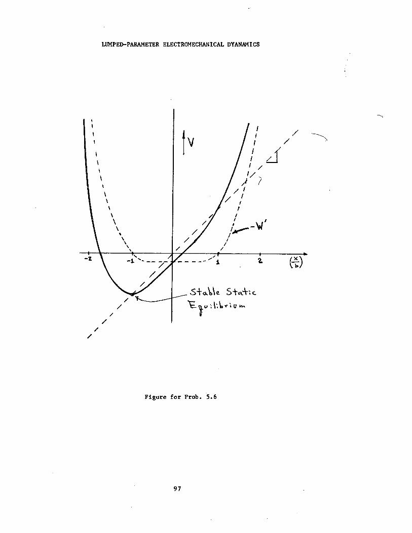
PROBLEM 5.6

Part a

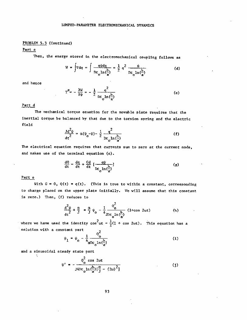
Questions of equilibrium and stability are of interest. Therefore, the

equation of motion is written in the standard form

M d 2 dt

x2 V (a) ax

where

V = Mgx - W' (b)

Here the contribution of W' to the potential is negative because Fe = aw'/ax.

The separate potentials are shown in the figure, together with the total

potential. From this plot it is clear that there will be one point of static

equilibrium as indicated.

Part b

An analytical expression for the point of equilibrium follows by setting

the force equal to zero

2L X av 2LX ~ Mg + 0 (c)

3x b 4

Solving for X, we have

4 1/3x =- [ ] (d)

2L I0

Part c

It is clear from the potential plot that the equilibrium is stable.

PROBLEM 5.7

From Prob. 3.15 the equation of motion is, for small 0

J K+ DN2 In( )I2 46 (a)dt2 2 o o )3

Thus, the system will have a stable static equilibrium at 0 = 0 if the

effective spring constant is positive, or if

221 DN b K > - in( ) (b)

)3 a o

LUMPED-PARAMETER ELECTROMECHANICAL DYANAMICS

I

IV II

1/

/1 /I

(~)

.a\e s +C ýc

k-,ý , " v W

Figure for Prob. 5.6

LUMPED-PARAMETER ELECTRCMECHANICAL DYNAMICS

PROBLEM 5.8

Part a

The coenergy is

W' = 1 )1(iO,x)di' + 12 X (il,i',x)di' (a) o o

which can be evaluated using the given terminal relations

' = [ i + Mil2 + L2i/( + x 3 (b)

T-1 1 M1 2 2 L2i2

If follows that the force of electrical origin is

fe = aW' 3 2 2i/

fe a[Llil + 2Mil2 + 2i/( + ) (c)

Part b

The static force equation takes the form

_fe = Mg (d)

or, with i2=02 and il1=I,

3 L1 1

2a X 4 Mg [1 + --o

Solution of this equation gives the required equilibrium position X

1 1/4Xo L I-a

= [ 2a

_ Mg

_ ] - 1 (f)

Part c

For small perturbations from the equilibrium defined by (e),

d2 x, 6L 1 2 x'M

o x2 6L

X 5= f(t) (g)

dt 2 + o) a

where f(t) is an external force acting in the x direction on M.

With the external force an impulse of magnitude I and the mass initially

at rest, one initial condition is x(O) = 0. The second is given by integrating

the equation of motion form 0 to 0+

+ + +

dt 0oddtl)dtdt - constant f0x'dt I. 0= .- 0 (t)dt (h)

0 0 0 0a

The first term is the jump in momentum at t=0, while the second is zero if

x is to remain continuous. By definition, the integral on the right is 0

Hence, from (h) the second initial condition is



MA ) =

Mo () = 0o x

In view of these conditions, the response is

(e - e ) X'(t) =

I2

where 117. x o 5~= aLl2aM'sr

a = LI2/a2M (1 + o

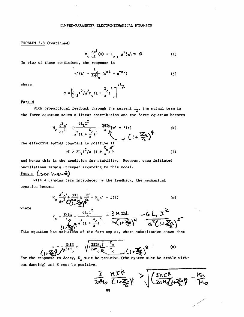
Part d

With proportional feedback through the current 12, the mutual term in

the force equation makes a linear contribution and the force equation becomes

d2x' 6L12 "4tM- 2 [ [ X - ]x' = f(t)"

0 dt a2 ( 1 + ao-)5- a The effective spring constant is positive if

? X% aI > 2L I /a (1 + -- ) M

1 a

and hence this is the condition for stability. However, once initiated

oscillations remain undamped according to this model.

Part e &5ee \• )

With a damping term introduced by the feedback, the mechanical

equation becomes

d2 x' 3MI4 dx'M + - + K x' = f(t)Sdt a t e

where

K 3MIa 6L 1 2 3 3:,4 -GLtI

2suX 5

a

This equation hias soluttns of the form exp st, where substitution shows that

e a the fho

s = 3MIB3M + (3MVI61 e (n) 2aM - 2aMo, Mo

For the response to decay, K must be positive (the system must be stable withe

out damping) and 6 must be positive.

23~4 n~IT > I-Ohc-

Ic~ic~P tFo

'7'7

LUMPED-PARAMETER ELECTRCMECHANICAL DYNAMICS

PROBLEM 5.9

Part a

The mechanical equation of motion is

M d 2 x = K(x-£ )-B + fe (a) dt S2 o dt

Part b

where the force fe is found from the coenergy function which is (because 1 2 1 32

the system is electrically linear) W' = Li2 = Ax i

fe = 3W'= 3 Ax 2 (b)f - = Ax i (b)

ax 2

Part c

We can both find the equilibrium points X and determine if they are stable 0

by writing the linearized equation at the outset. Hence, we let x(t)=X +x'(t)

and (a) and (b) combine to give

dd2 x'x dx' 3 2 2M - K(Xo-Po)-Kx' - B + - AI (X + 2X x') (c) dtdt

2 0 0 dt 2 o + 0

With the given condition on 1o, the constant (equilibrium) part of this equation

is 3X2

X - o (d)o o 16Z

0

which can be solved for X /Z, to obtaino o

x 12/3 o 1/3 (e)

That is, there are two possible equilibrium positions. The perturbation part

of (c) tells whether or not these are stable. That equation, upon substitution

of Xo and the given value of Io, becomes

d2 x' 3/2 dx'M _2 - -K[l- (

1/2)]x' - B

dt (f) dt

where the two possibilities correspond to the two equilibrium noints. Hence,

we conclude that the effective spring constant is positive (and the system is

stable) at XO/k = 4/3 and the effective spring constant is negative (and hence

the equilibrium is unstable) at X /0o = 4.

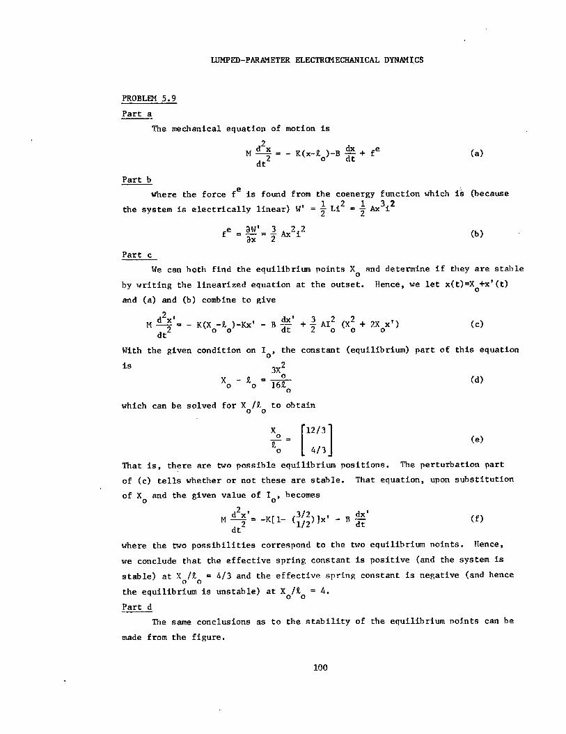
Part d

The same conclusions as to the stability of the equilibrium noints can be

made from the figure.



T

Consider the equilibrium at Xo = 4. A small displacement to the right makes

the force fe dominate the spring force, and this tends to carry the mass

further in the x direction. Hence, this point is unstable. Similar arguments

show that the other point is stable.

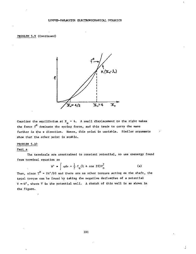
PROBLEM 5.10

Part a

The terminals are constrained to constant potential, so use coenergy found

from terminal equation as

W' = qdv = -4 (l + cos 2e)V22o o

Then, since Te = aW'/ae and there are no other torques acting on the shaft, the

total torque can be found by taking the negative derivative of a potential

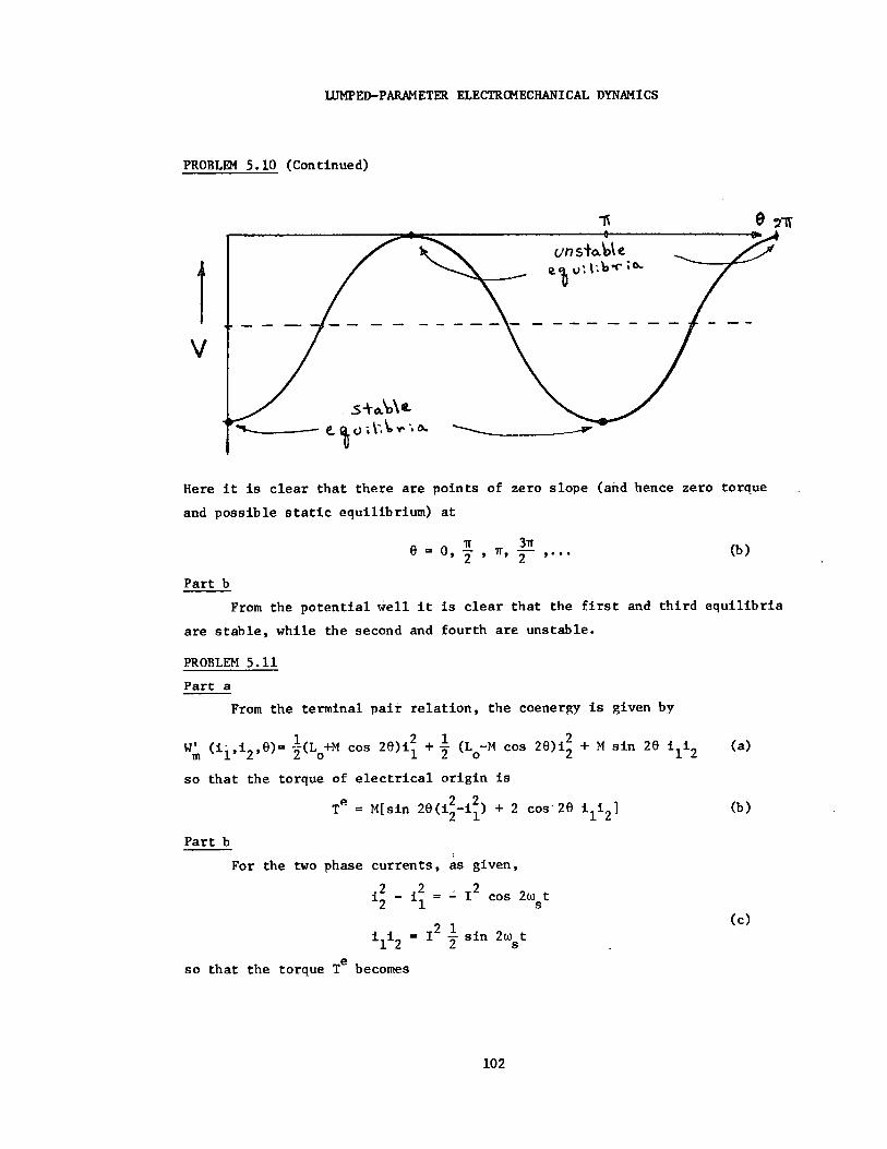
V =-W', where V is the potential well. A sketch of this well is as shown in

the figure.

JUMPED-PARAMETER ELECTROMECHANICAL DYNAMICS


I V

SSa~b\C

~c~-.$ c~;~lb~;a

Here it is clear that there are points of zero slope (and hence zero torque

and possible static equilibrium) at

e= o0o 7, 3r

Part b

From the potential well it is clear that the first and third equilibria

are stable, while the second and fourth are unstable.

PROBLEM 5.11

Part a

From the terminal pair relation, the coenergy is given by

Wm (ii,i2'e)= (Lo+M cos 20)il + (Lo-M cos 20) 2 + M sin 2i ili2

so that the torque of electrical origin is

Te = M[sin 20(i 2-i1 ) + 2 cos 26 ili22 1 1 21

Part b

For the two phase currents, as given,

2 2 12i _ i1 I cos 2w t 2 1 s

i1 2 1 sin 2w t 1 2 s

so that the torque Te becomes



Te = MI2 [-sin 20 cos 2w t + sin 2wst cos 20] (d)

or

Te = MI2sin(2 s t - 20) (e)

Substitution of 6 w t + 6 obtains m

Te 2

T= - MI sin[2(wm-w)t + 2] (f)

and for this torque to be constant, we must have the frequency condition

W m =W

s (g)

under which condition, the torque can be written as

Te = - MI2sin 26 (h)

Part c

To determine the possible equilibrium angles 60, the perturbations and

time derivatives are set to zero in the mechanical equations of motion.

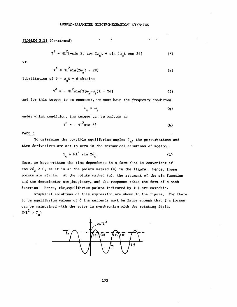
T = MI 2 sin 26 (i)o o

Here, we have written the time dependence in a form that is convenient if

cos 260 > 0, as it is at the points marked (s) in the figure. Hence, these

points are stable. At the points marked (u), the argument of the sin function

and the denominator are,imaginary, and the response takes the form of a sinh

function. Hence, the/equilibrium points indicated by (u) are unstable.

Graphical solutions of this expression are shown in the figure. For there

to be equilibrium values of 6 the currents must be large enough that the torque

can be maintained with the rotor in synchronism with the rotating field.

(MI > T )

MAI 2 r

76 maa

VIA



Returning to the perturbation part of the equation of motion with wm = us,

J 2 (Wt + 6 + 6') = T + T' - MI2 sin(26 + 26') (j) dt 2 m o o odt

linearization gives

J A-+ (2MI2 cos 26~)6' = T' (k) dt 2

where the constant terms cancel out by virtue of (i). With T' = Tuo(t) and

initial rest conditions,the initial conditions are

* ( 0+ ) = -o (1)

dt J

6'(0 + ) = 0 (m)

and hence the solution for 6'(t) is

S2MI 2 cos 26 6'(t) = o sin o t (n)

2MI2cos 26

PROBLEM 5.12

Part a

The magnitude of the field intensity\ (H) in the gaps is the same. Hence,

from Ampere's law,

H = Ni/2x (a)

and the flux linked by the terminals is N times that passing across either

of the gaps.

~ adN2

= i = L(x)i (b)2x

Because the system is electrically linear, W'(i,x) = 1

Li 2 2 , and we have.

2

fe = N2ad=o i 2 (c)ax 2

4x

as the required force of electrical origin acting in the x direction.

Part b

Taking into account the forces due to the springs, gravity and the

magnetic field, the force equation becomes

104

LUMPED-PARAMETER ELECTRGCECHANICAL DYNAMICS


2 N2ado

M 2 = - 2Kx + Mg 2 i + f(t) (d) dt 4x 2

where the last term accounts for the driving force.

The electrical equation requires that the currents sum to zero at the

electrical node, where the voltage is dA/dt, with X given by (b).

I adN2I

R dt [ •

2x i] + i (e)

Part c

In static equilibrium, the electrical equation reduces to i=I, while

the mechanical equation which takes the form fl f2 is satisfied if2 2

N2adj o12

-2KX + Mg = (f) 4X

Here, f2 is the negative of the force of electrical origin and therefore

(if positive) acts in the - x direction. The respective sides of (f) are

shown in the sketch, where the points of possible static equilibrium are

indicated. Point (1) is stable, because a small excursion to the right makes

f2 dominate over fl and this tends to return the mass in the minus x direction

toward the equilibrium point. By contrast, equilibrium point (2) is

characterized by having a larger force f2 and fl for small excursions to the

left. Hence, the dominate force tends to carry the mass even further from the

point of equilibrium and the situation is unstable. In what follows, x = X

will be used to indicate the position of stable static equilibrium (1).



Part d

If R is very large, then

i : I

even under dynamic conditions. This approximation allows the removal of

the characteristic time L/R from the analysis as reflected in the

reduction in the order of differential equation required to define the

dynamics. The mechanical response is determined by the mechanical

equation (x = X + x')

M-d2 2 x x' = - 2Kx' +

N adpo0I

22 x' + f(t) (g) dt2 2X3

where the constant terms have been balanced out and small perturbations are

assumed. In view of the form taken by the excitation, assume x = Re x ejet .and define Ke E 2K - N2adoI2/2X3 Then, (g) shows that

S= f/(Ke-0M) (h)

To compute the output voltage

S p 0a d N2 1 dx'd

o dt i= 22 dti=I =i

orupor adN2 I

=2 x (0) o2X

Then, from (h), the transfer function is

2v w0 adN I

o o j (k)

f 2X2 (Ke2jM)

PROBLEM 5.13

Part a

The system is electrically linear. Hence, the coenergy takes the

standard form

W' 1 L 1

22 +L ii + 11 L 122 (a)

2 111 1212 2 222(a)

and it follows that the force of electrical origin on the plunger is

Sx = i + i l22 + 2i2 (b)ax 2 1 x 1 2 3x 2 2 ax



which, for the particular terminal relations of this problem becomes

2 2-if ilix2 i

fe L { (+ x_ 1 2x 2 ( x (c)o d d d d d dc)

Finally, in terms of this force, the mechanical equation of motion is

2d2--2 = -Kx - B T- + fe (d)

dtdt

The circuit connections show that the currents i1 and 12 are related to the

source currents by

i = I + i (e) 1 =o -i

Part b

If we use (e) in (b) and linearize, it follows that

4L I 4L 12fe oo oo (f)

d d d

and the equation of motion is

dx dx 22 + a - +wx= - Ci (g)dt dt o

where

4L 12 ao = [K + ]/M

2 o

a = B/M

C = 4L I /dM

Part c

Both the spring constant and damping in the equation of motion are

positive, and hence the system is always stable.

Part d

The homogeneous equation has solutions of the form ept where

p 2 + ap + 2 = 0 (h)0

or, since the system is underdamped

a 2 2 a)•

p = - 2 + J - (i)2 - 02 p

LUMPED-PARAMETER ELECTROM4ECHANICAL DYNAMICS

PROBLE~ 5.13 (Continued)

The general solution is

CI t x(t) = - + e [A sin w t + D cos w t] (j)

2 p p o

where the constants are determined by the initial conditions x(O) = 0 and

dx/dt(O) = 0

CI tCI D =--

o ; A =

o (k)

w 2w w o po

Part e

With a sinusoidal steady state condition, assume x = Re x e and write

i(t) = Re(-jI )ej t and (g) becomes

- 2 2 )x(-w + jwa + = Cj (1)

Thus, the required solution is

RejCI e t

x(t) ( 2 2 (m)

0

PROBLEM 5.14

Part a

From the terminal equations, the current ii is determined by Kirchhoff's

current lawdi

G L di+ i = I + CMI sin Pt (a)G1 dt 1 2

The first term in this expression is the current which flows through G because

of the voltage developed across the self inductance of the coil, while the last

is a current through G induced bhv the rotational motion. The terms on the right

are known functions of time, and constitute a driving function for the linear

equation.

Part b

We can divide the solution into particular solutions due to the two driving

terms and a homogeneous solution. From the constant drive I we have the solution

i I = I (b)

Because sin Pt = Re(-jej t), if we assume a particular solution for the

) we havesinusoidal drive of the form i1 = Re(Ie(I ), we have


PROBLEK 5.14 (Continued)

11 (jDGL 1 + 1) = - J~GMI 2 (c)

or, rearranging

-OGMI 2 (GCL1 + j) 1 +( 1) 2 (d)

We now multiply this complex amplitude by ejot and take the real .part to

obtain the particular solution due to the sinusoidal drive

-GMI2l1 1 2 (QGL1 cos Pt - sin Qt) (e)

1+(PGLI)

The homogeneous solution is

-t/GL 1

t1 = Ae (f)

and the total solution is the sum of (b), (e) and (f)with the constant A

determined by the initial conditions.

In view of the initial conditions, the complete solution for il, normalized

to the value necessary to produce a flux equal to the maximum mutual flux, is

then

Llil 1e LMI Q(tGLI) 1

MI 2 2 1+(GL ) 2

+ GL1R 2 (sin t - GGL L1I L+(QG2L1 )

11 cos Qt) +

MI2 (g)

Part c

The terminal relation is used to find the flux linking coil 1 l GLI) 2 LI 1

MI2 I+I(GL ) M 2 t

GLIQ LIG~1R cos Rt 1

2 ( L 2 MI1+(QGLI) 1+( GL1) 2

The flux has been normalized with respect to the maximum mutual flux (MI2).



Part d

In order to identify the limiting cases and the appropriate approximations

it is useful to plot (g) and (h) as functions of time. These equations contain

two constants, QGL1 and L I/MI2 . The time required for one rotation is 2r/S and

GL1 is the time constant of the inductance L1 and conductance G in series. Thus,

QGL1 is essentially the ratio of an electrical time constant to the time required

for the coil to traverse the applied field one time. The quantity MI2 is the

maximum flux of the externally applied field that can link the rotatable coil and

I1I is the self flux of the coil due to current I acting alone. Thus, I1I/MI 2

is' the ratio of self excitation to mutual excitation.

To first consider the limiting case that can be approximated by a current

source we require that

L1I QGL <<

1 1 and GL << MI

1 MI2 (i)

To demonstrate this set

LI WGL = 0.1 and -- = 1 (j)

1 MI

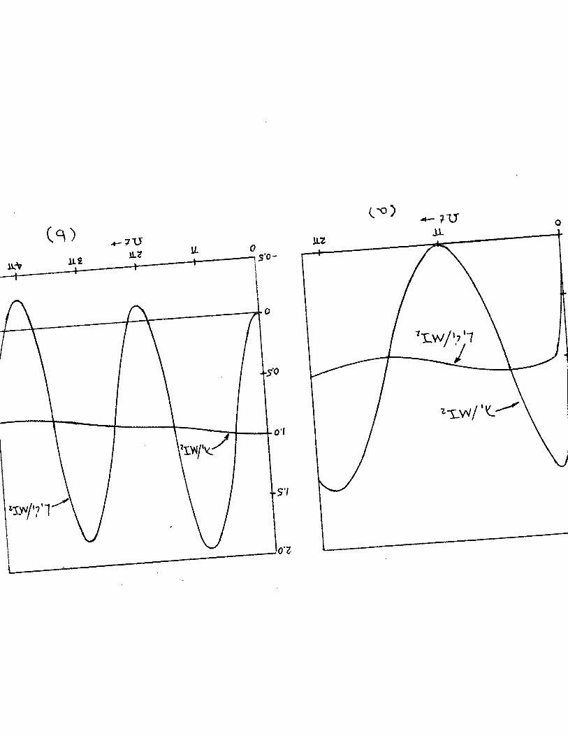
and plot current and flux as shown in Fig. (a). We note first that the

transient dies out very quickly compared to the time of one rotation. Further

more, -the flux varies appreciably while the current varies very little compared

to its average value. In the ideal limit (GqO) the transient would die out

instantaneously and the current would be constant. Thus the approximation of

the situation by an ideal current-source excitation would involve a small

error; however, the saving in analytical time is often well worth the decrease

in accuracy resulting from the approximation.

Part e

We next consider the limiting case that can be approximated by a constant-

flux constraint. This requires that

QGL1 >> 1 (k)

To study this case, set

CGL1 = 50 and I = 0 (1)

The resulting curves of flux and current are shown plotted in Fig. (b).

Note that with this constraint the current varies drastically but the flux

pulsates only slightly about a value that decays slowly compared to a rotational

period. Thus, when considering events that occur in a time interval comparable

C-)

rs

I-Di

(-O) 4-;U

CA~)

LUMPED-PARAMETER ELECTR(OMECHANICAL DYNAMICS


with the rotational period, we can approximate this system with a constant-flux

constraint. In the ideal, limiting 6ase, which can be approached with super

conductors, G-m and X1 stays constant at its initial value. This initial value

is the flux that links the coil at the instant the switch S is closed.

In the limiting cases of constant-current and constant flux constraints

the losses in the electrical circuit go to zero. This fact allows us to take

advantage of the conservative character of lossless systems, as discussed in

Sec. 5.2.1.

Part f

Between the two limiting cases of constant-current and constant flux

constraints the conductance G is finite and provides electrical damping on

the mechanical system. We can show this by demonstrating that mechanical

power supplied by the speed source is dissipated in the conductance G. For

this purpose we need to evaluate the torque supplied by the speed source.

Because the rotational velocity is constant, we have

Tm= - Te (m)

The torque of electrical origin Te is in turn

aW'(il, i 22, ) Te = (n)

Because the system is electrically linear, the coenergy W' is

W' Li + M i + L2 (o)2 1 1 1 2 2 2 2 Co)

and therefore,

Te = - M i 12 sin 6 (p)

The power supplied by the torque Tm to rotate the coil is

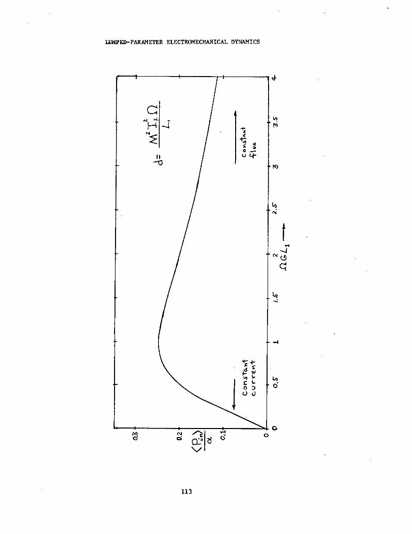
Pin - T d = I sin Qt (W)Mil2

Part g

Hence, from (p) and (q), it follows that in the sinusoidal steady state

the average power <P. > supplied by the external toraue is in

<Pin > = 1 (r)

in 2


to

-Ir trl c,,

O

-0


PROBLFM 5.14 (Continued)

This power, which is dissipated in the conductance G, is plotted as a function

of ~2GL 1 in Fig. (c). Note that because 0 and L1 are used as normalizing

constants, ?GL 1 can only be varied bhv varving G. Note that for both large and

small values of fGT.1 the average mechanical power dissipated in G becomes small.

The maximum in <Pin > occurs at GCL 1 = 1.

PROBLEM 5.15

Part a

The coenergy of the capacitor is

= C(x) V2 = 1 (EA )V2 e 2 2 ox

The electric force in the x direction is

aW' EA e 1 o 2

e ýx 2 2 x

If this force is linearized around x = xo, V = V

f (x)e

=0 1 2

1 AV' o o

2

1)2 E AV v

o o0

2 +

2 E AV x

o o0 03

x x x O O O

The linearized equation of motion is then

AV 2

dx ++ (K-E

)xo) -c A

0V v + f(t)B -ý0 ' = V

dt 3 2 o x x

0 0

The equation for the electric circuit is

d V + R -6 (C(x)V) = V

Part b

We can keep the voltage constant if

R -- 0

In this case AV2

B dx + K'x = f(t) = F ul(t); K' = K 0 3 x

The particular solution is

=x(t) F/K'



The natural frequency S is the solution to

SB +K'x = 0 $ = - K'/B

Notice that since Z

E AV

X'/B = (K- 3)/B X(t)x0 F

Sr- /d there is voltage V above which the

system is unstable. Assuming V isO

less than this voltage t

-x(t) = F/K' (1-e (K ' / B)t)

Now we can be more specific about the size of R. We want the time

constant of the RC circuit to be small compared to the "action time" of the

mechanical system

RC(xo) << B/K'

B

R << BK'C(xo)

Part c

From part a we suspect that

RC(xo) >> Tmech

where Tmech can be found by letting R + m. Since the charge will be constant

d = 0 q = C(x )V = C(X +X)(V +V)dt 00 0 0

dC- C(xo)V + C(xo)v + Vo 4-c (xo)x

V Vx EA v (oo dC- (x

) x - + oo o x Vx x

C(x) dxxo)X E A 2 ox o

Using this expression for induced v, the linearized equation of motion

becomesSAV2 Adxo o o0 2

B + (K- )x - V x +f(t)dt 3 3 o

x x o o

dxB dx + Kx = f(t)

dt



The electric effect disappears because the force of a capacitor with

constant charge is independent of the plate separation. The solutions are the

same as part (a) except that K' = K. The constraint on the resistor is then

R >> 1 B/KC(xo)

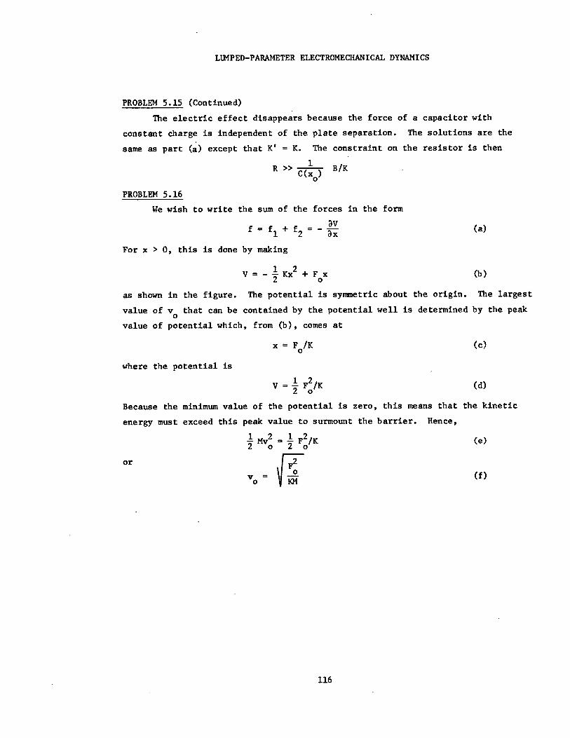
PROBLEM 5.16

We wish to write the sum of the forces in the form

f f + f aV

(a)1 2 3x

For x > 0, this is done by making

1 2V Kx + Fx (b)

2 o

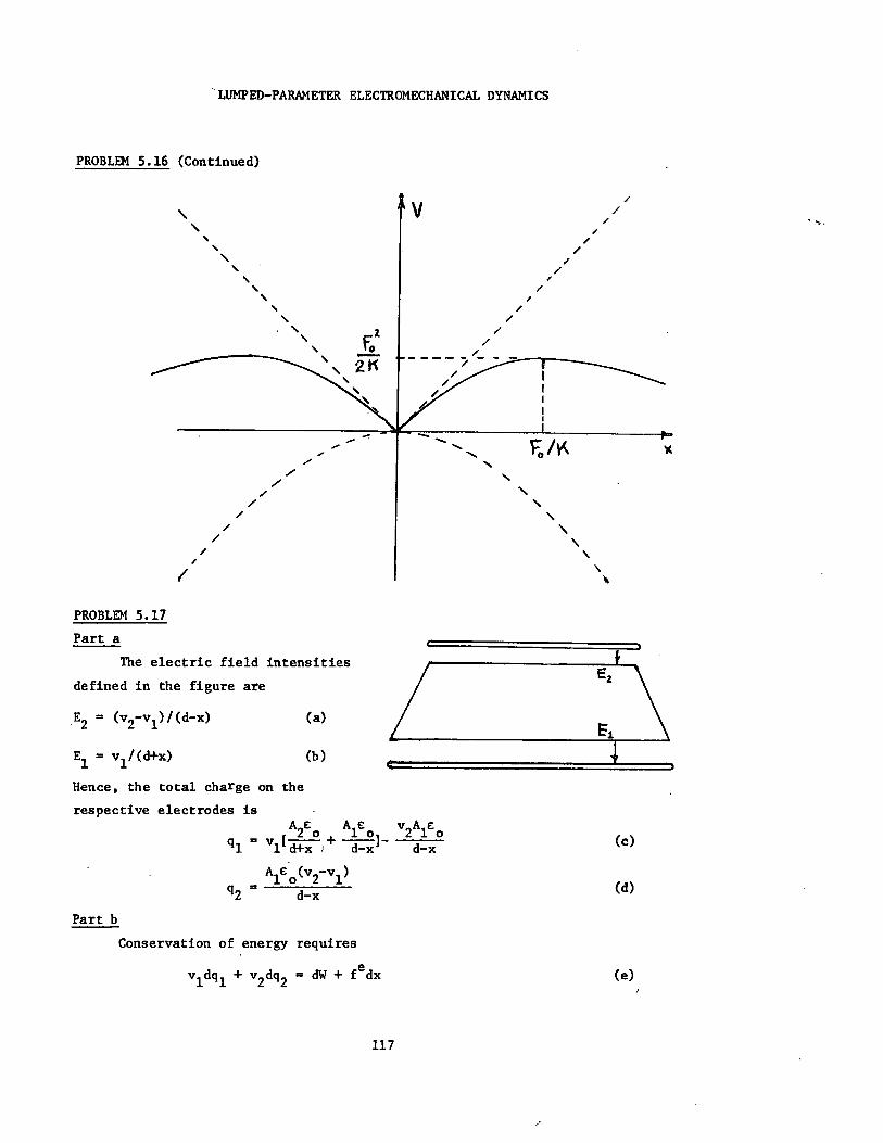
as shown in the figure. The potential is symmetric about the origin. The largest

value of vo that can be contained by the potential well is determined by the peak

value of potential which, from (b), comes at

x = Fo/K (c)

where the potential is

V = 1 F2/K (d)2 o

Because the minimum value of the potential is zero, this means that the kinetic

energy must exceed this peak value to surmount the barrier. Hence,

SMv2 I F2/K (e)2 o 2 o

or F2

vo= (f)



PROBLEM 5.17

Part a

The electric field intensities

defined in the figure are

E2 = (v2-v1)/(d-x) /

I E\

E 1

= v,/(d+x)1

Hence, the total charge on the

respective electrodes is

q= S

`2

A2E o v1 [. 0+Vl[d+x +

AIC (v2-v

d-x

A

)

o 0 -x]-

v2A1E o o

d-x

Part b

Conservation of energy requires

vldq1 + v2dq2 = dW + fedx


and since the charge q1 and voltage v2 are constrained, we make the

transformation v2dq2 = d(v2q2)-q2 dv2 to obtain

v1 dql-q 2 dv 2 = dW" + fedx (f)

It follows from this form of the conservation of energy equation thatfe W fe= - • and hence W" H U. To find the desired function we integrate

(f) using the terminal relations.

U = W"= dql - q2dv 2 (g)

The integration on q1 makes no contribution since ql is constrained to be

zero. We require v2(ql=0,v 2) to evaluate the remaining integral

v2A1i Io1 1 (h) q 2 (q 1 0,v 2) d-x 1- A2(dx ) (h)

SAl(d+x)

Then, from (g),

U 1 0 1 o 1U V 1 (i)2 d-x A2 (d-x)

A5(d+x) 1

PROBLEM 5.18

Part a I

Because the two outer plates are X

constrained differently once the switch

is opened, it is convenient to work in

terms of two electrical terminal pairs,

defined as shown in the figure. The

plane parallel geometry makes it

straightforward to compute the

terminal relations as being those for

simple parallel plate capacitors, with

no mutual capacitance.

ql 1 x (a)VlEoA/a +

q2 V2 oA/a-x (b)

+, ~o 2)~ '4 00



Conservation of energy for the electromechanical coupling requires

v1dql+ v2 dq2 = dW + fedx (c)

This is written in a form where q1 and v2 are the independent variables by

using the transformation v2dq2 = d(v2q2)-q2dv2 and defining W"qW-v2q 2

v1dq1 - 2dv2 dW" + fedx (d)

This is done because after the switch is opened it is these variables that

are conserved. In fact, for t > 0,

v2 = V and (from (a))ql = VoeoA/a (e)

The energy function W" follows from (d) and the terminal conditions, as

W" = vldql- fq2 dv 2 (f)

or

c Av2 1 (a+x) 2 1 oAV2

q -(g)2 cA q1 2 a-xo

Hence, for t > 0, we have (from (e))

AV2 E AV22

1 (a+x) 1 oAV2 2 o A 2 a-x

aPart b

e aW"The electrical force on the plate is fe W" Hence, the force

equation is (assuming a mass M for the plate)

2, EoAV2 E AV2dx 1 o o 1 o oM - Kx + (i)

dt a (a-x)

For small excursions about the origin, this can be written as 2 cAV2 EAV2 cAV2

dx 1 o 0 o o 01o oM- 2 -Kx-2 2 + 2 2 + 3 x (j)

dt a a a

The constant terms balance, showing that a static equilibrium at the origin

is possible. Then, the system is stable if the effective spring constant

is positive.

K > c AV2/a3 (k)0 0

Part c

The total potential V(x) for the system is the sum of W" and the

potential energy stored in the springs. That is,


PROBLEM 5.18 (Continued)2

1 2 1 (a+x) AV 1 E AV

o 2 2 2 o o 2 a-x

a

2 2 EAV 2 aKK1 oo x 1

2 ( 2 a a x (1- )

a

This is sketched in the figure for a2K/2 = 2 and 1/2 c AV2/a = 1. In additiono o

to the point of stable equilibrium at the origin, there is also an unstable

equilibrium point just to the right of the origin.

PROBLEM 5.19

Part a

The coenergy is

W' Li = i /1 - -42 2 ao

and hence the fbrce of electrical origin is

'

e dw4f = 2L iL/a[l x o a

Hence, the mechanical equation of motion, written as a function of (i,x) is

S21,22 2L _i

d xM = - Mg +

dt a[1- -a a



while the electrical loop equation, written in terms of these same variables

(using the terminal relation for X) is

VVo + v = Ri + dt - [ (1-- )(d) (d)

a

These last two expressions are the equations of motion for the mass.

Part b

In static equilibrium, the above equations are satisfied by (x,v,i) having

the respective values (Xo,VoIo). Hence, we assume that

x = Xo + x'(t): v = Vo + v(t): i = Io + i'(t) (e)

The equilibrium part of (c) is then

2L 12 X 5 0 - Mg + a o/(1 - o) (f)a a

while the perturbations from this equilibrium are governed by

2 x 10 L 12 x' 4 LI i' M d

2 +

X 6 + X 5 (g)

a (l- -) a(l- 0-)a a

The equilibrium part of (d) is simply Vo = I R, and the perturbation part is

L di* 4 LI v = Ri' + 0 d+ 00 (h)X 4 dt X 5 dt

[1- •-1] al- -o]a a

Equations (g) and (h) are the linearized equations of motion for the system which

can be solved given the driving function v(t) and (if the transient is of interest)

the initial conditions.

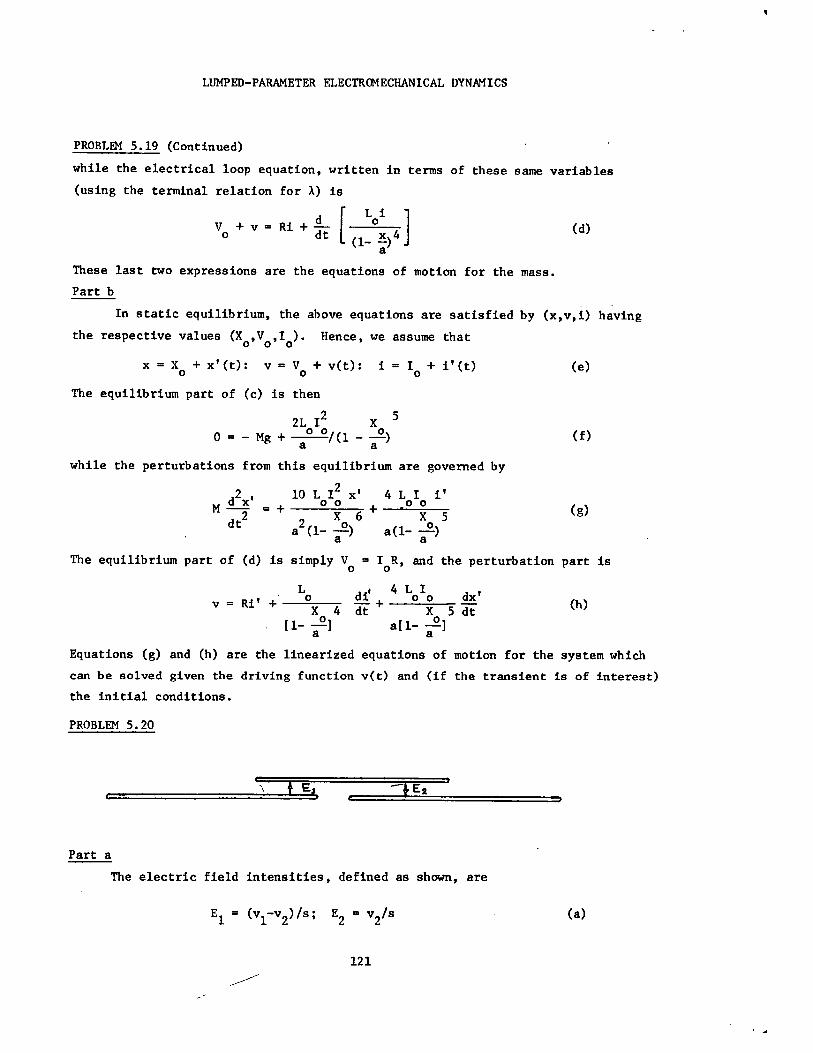
PROBLEM 5.20

Part a

The electric field intensities, defined as shown, are

E1 = (V 1-V2 )/s; E2 = v2/s (a)

121



In terms of these quantities, the charges are

= q 1 Eo( - x)dE1 ; q2 - o( -x)dE + o( + x)dE2 (b)

Combining (a) and (b), we have the required terminal relations

q = V1C11 - v2C12 (c)

q2 =V 1 12 + V2C22

whereEd E ad o a o

C11 = - (- x); C22ii s 22 s Ed o a

C12 s (

For the next part it is convenient to write these as q1(vl,q2) and v2(v ,q 2).

2

1 v1 [C1 1 C2 2 C2 q 22 22

q 2 C12 (d)v + v 2 C 1 C22 22

Part b

Conservation of energy for the coupling requires

v1dql + v2dq2 = dW + fedx (e)

To treat v1 and q2 as independent variables (since they are constrained to be

constant) we let vldq1 = d(vlql)-q dvl, and write (e) as

-ql dv1 + v2dq2 = - dW" + fe dx (f)

From this expression it is clear that fe = aW"/,x as required. In particular,

the function W" is found by integrating (f)

W" = o l(,O)dv' - v 2 (Vo,q)dq2 (g) o o

to obtain

C2 2 V OC = 1 V2[C _ Q o 12 (h)

2 o 11 C1 2 ] 2C22C22 C22

Of course, C1 1, C22 and C12 are functions of x as defined in (c).


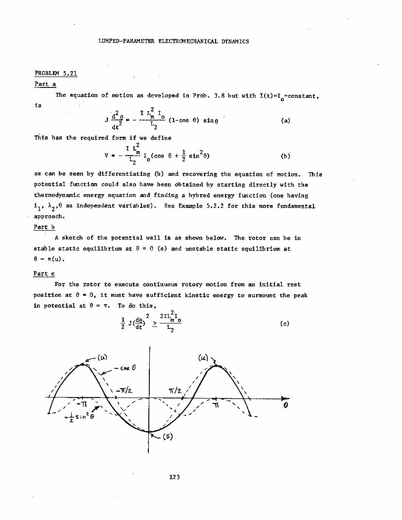
PROBLEM 5.21

Part a

The equation of motion as developed in Prob. 3.8 but with I(t)=Io=constant,

is 2 I L2 1

J dt2

d - m L2

(1-cos 6) sine (a) dt 2

This has the required form if we define

IL m 1 2

V L (cos 0 + sin 0) (b)

as can be seen by differentiating (b) and recovering the equation of motion. This

potential function could also have been obtained by starting directly with the

thermodynamic energy equation and finding a hybred energy function (one having

il' X2,6 as independent variables). See Example 5.2.2 for this more fundamental

approach.

Part b

A sketch of the potential well is as shown below. The rotor can be in

stable static equilibrium at e = 0 (s) and unstable static equilibrium at

S= r(u).

Part c

For the rotor to execute continuous rotory motion from an initial rest

position at 0 = 0, it must have sufficient kinetic energy to surmount the peak

in potential at 8 = W. To do this,

2 2IL211 j (Lmo 2

Jt dt

-- L

•> (c)

- c


PROBLEM 5.22

Part a

The coenergy stored in the magnetic coupling is simply

W'= Lo(l + 0.2 cos 0 + 0.05 cos 268) 2 (a)

Since the gravitational field exerts a torque on the pendulum given by

T = (-Mg X cose) (b)p ae

and the torque of electrical origin is Te = ~W'/~8, the mechanical equation of

motion is

d ro [t 2 2 + V =0 (c)

where (because I 2 Lo 6MgZ)

V = Mgt[0.4 cos e - 0.15 cos 20 - 3]

Part b

The potential distribution V is plotted in the figure, where it is evident

that there is a point of stable static equilibrium at 0 = 0 (the pendulum

straight up) and two points of unstable static equilibrium to either side of

center. The constant contribution has been ignored in the plot because it is

arbitrary.

strale

I \

C/h ~ta I


PROBLEM 5.23

Part a

The magnetic field intensity is uniform over the cross section and equal

to the surface current flowing around the circuit. Define H as into the paper

and H = i/D. Then X is H multiplied by Uo and the area xd.

p xd -- i (a)

The system is electrically linear and so the energy is W X2 L. Then, since

fe = _ aW/ax, the equation of motion is

d2x 1 A2DM d 2 x

dt2 = f f - Kx + D (b)

2 2

Part b

Let x = X + x'where x' is small and (b) becomes approximately

d2x' 1 A2 D A2Dx'M

dt2 x 2 = -KX - Kx' + (c)

o 2 2d oX3d 00

The constant terms define the static equilibrium

1 A2D 1/3X° = [ ]K- (d)

o

and if we use this expression for Xo, the perturbation equation becomes,

d22x'M = -Kx' - 2Kx' (e)dt2

Hence, the point of equilibrium at Xo as given by (d) is stable, and the magnetic

field is equivalent to the spring constant 2K.

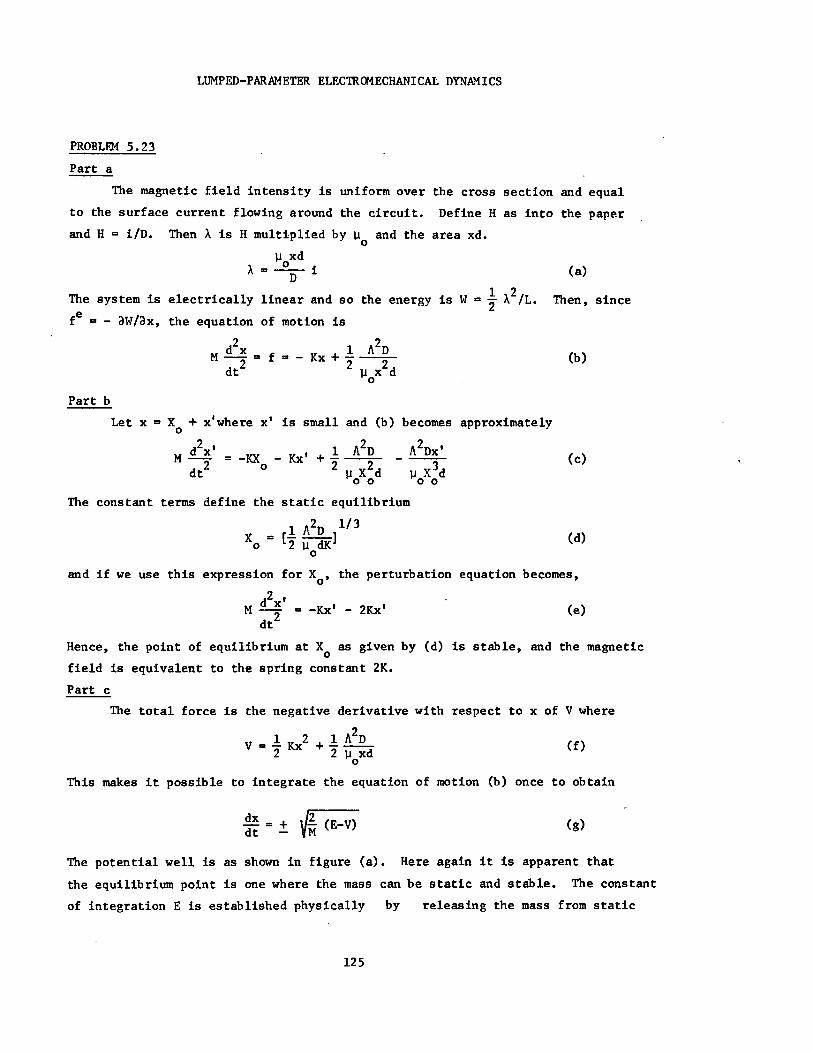
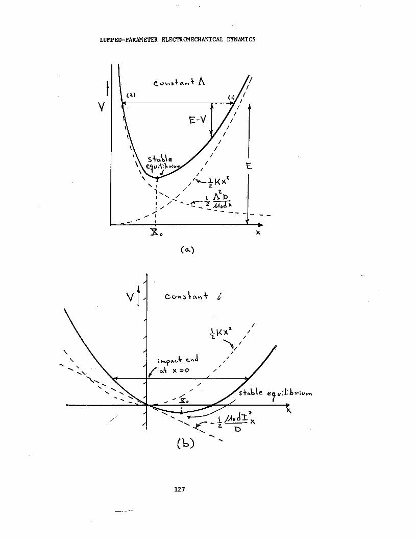
Part c

The total force is the negative derivative with respect to x of V where

1 2 1 A2DV = Kx + A-D (f)

2 2jixd

This makes it possible to integrate the equation of motion (b) once to obtain

d= + 2 (E-V) (g)dt -M

The potential well is as shown in figure (a). Here again it is apparent that

the equilibrium point is one where the mass can be static and stable. The constant

of integration E is established physically by releasing the mass from static



positions such as (1) or (2) shown in Fig. (a). Then the bounded excursions of

the mass can be pictured as having the level E shown in the diagram. The motions

are periodic in nature regardless of the initial position or velocity.

Part d

The constant flux dynamics can be contrasted with those occurring at

constant current simply by replacing the energy function with the coenergy

function. That is, with the constant current constraint, it is appropriate to find

the electrical force from W' = Li2 ' where fe = W'/ax. Hence, in this case

1 2 1 oxd 2 (h) 2 2 D

A plot of this potential well is shown in Fig. (b). Once again there is a point

X of stable static equilibrium given by

X 1 d 2 (i)o 2 DK

However, note that if oscillations of sufficiently large amplitude are initiated

that it is now possible for the plate to hit the bottom of the parallel plate

system at x = 0.

PROBLEM 5.25

Part a

Force on the capacitor plate is simply

wa2 2 fe 3W' 3 1 o (a)

f • x x 21 x

due to the electric field and a force f due to the attached string.

Part b

With the mass M1 rotating at a constant angular velocity, the force fe

must balance the centrifugal force Wm rM1 transmitted to the capacitor plate

by the string.

wa2E V2 1 oo = 2 (b) 2 2 m 1

or \Ia a2 V2

= 0 (c)m 2 £3M1

where t is both the equilibrium spacing of the plates and the equilibrium radius

of the trajectory for M1.


(0,)

OA x---aco s %~ -0

oY\

V~x r

(b)



Part c

The e directed force equation is (see Prob. 2.8) for the accleration

on a particle in circular coordinates)

d2 eM 1[r d2 + 2

dr d6dt dt = 0 (d)

dt

which can be written as

d 2 dOdt [M1r d- 1= 0 (e)

This shows that the angular momentum is constant even as the mass M1 moves in and

out

2 de 2 M1d m =M r = . constant of the motion (f)

This result simply shows that if the radius increases, the angular velocity must

decrease accordingly

de 2 dt 2 ()

r

Part d

The radial component of the force equation for M1 is

2 2 Ml[d - r-) ]= - f (h)

dt

where f is the force transmitted by the string, as shown in the figure.

S( i grv\,

The force equation for the capacitor plate is

Mdr e(i) dt

where fe is supplied by (a) with v = V = constant. Hence, these last two o

expressions can be added to eliminate f and obtain

--



2 a 2C 2V2 d w(M1++ 2 - r ) = 1 o oa (j)1 2.

dt 1 Tr ro 0,

If we further use (g) to eliminate d6/dt, we obtain an expression for r(t)

that can be written in the standard form

2(M1 2 2 V = 0 (k)

2 dt

where M 4 2 7a2 2

V = 2 (1)2 r

2r

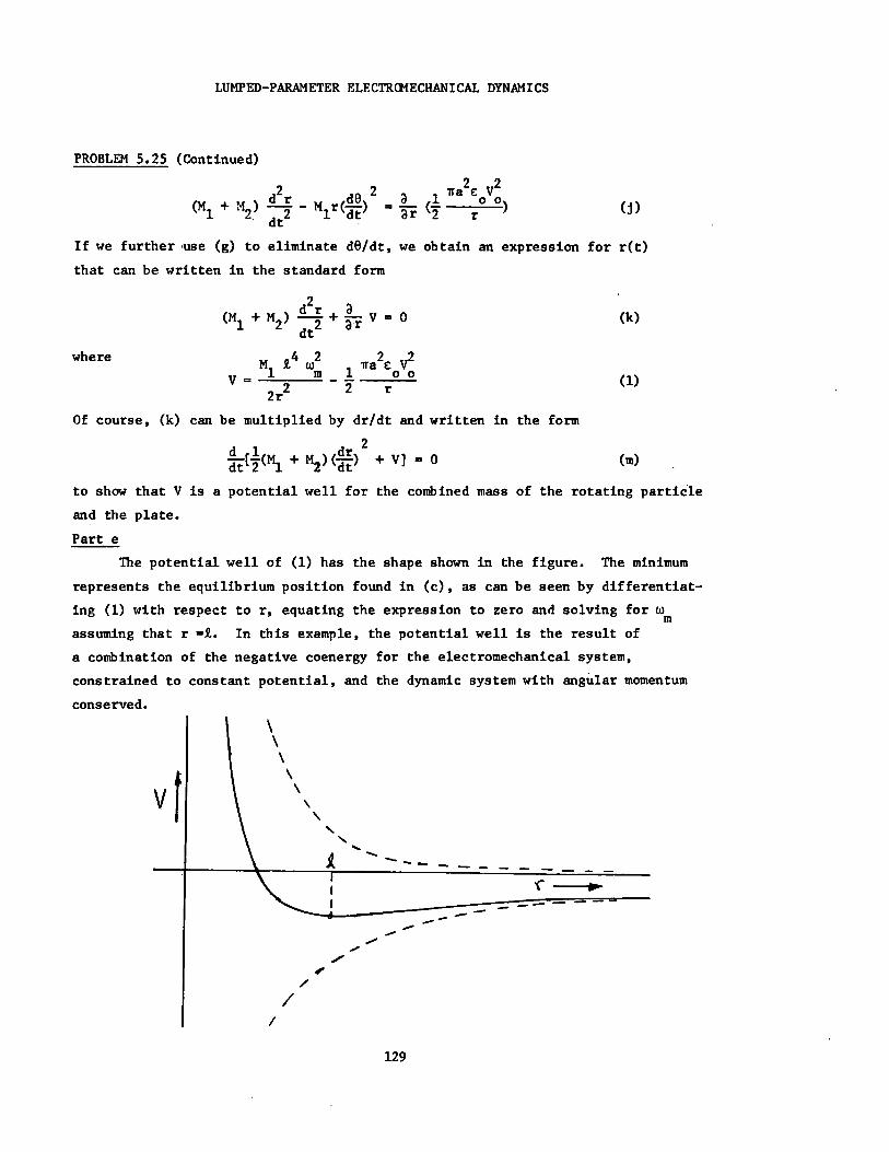
Of course, (k) can be multiplied by dr/dt and written in the form

d 1 dr1 S(M + V] =0 (m)2)(

to show that V is a potential well for the combined mass of the rotating particle

and the plate.

Part e

The potential well of (1) has the shape shown in the figure. The minimum

represents the equilibrium position found in (c), as can be seen by differentiat

ing (1) with respect to r, equating the expression to zero and solving for wm assuming that r =£. In this example, the potential well is the result of

a combination of the negative coenergy for the electromechanical system,

constrained to constant potential, and the dynamic system with angular momentum

conserved.


PROBLEM 5.26

Part a

To begin the analysis we first write the Kirchhoff voltage equations for

the two electric circuits with switch S closed

dX V = ilR1 + (a)

dX20 = i2R 2 dtd),

(b)

To obtain the electrical terminal relations for the system we neglect fringing

fields and assume infinite permeability for the magnetic material to obtain*

1 = N1 ' 2 = N24 (c)

where the flux $ through the coils is given by

21o wd (N1 1 + N2i2)$ = (d)

g(l + -)

We can also use (c) and (d) to calculate the stored magnetic energy as**

g(l + x) 2 W = (e)

m 4 ° wd

We now multiply (a) by N1/R1 and (b) by N 2/R2, add the results and use

(c) and (d) to obtain

x 2 2NV g(l+ -) N N1V1 + (- + 2) (f) R1 21 wd R1 R2 dt

Note that we have only one electrical unknown, the flux 0, and if the plunger is

at rest (x = constant) this equation has constant coefficients.

The neglect of fringing fields makes the two windings unity coupled. In practicethere will be small fringing fields that cause leakage inductances. However,these leakage inductances affect only the initial part of the transient andneglecting them causes negligible error when calculating the closing time of

the relay.

**Here we have used the equation QplPg)b W =iL 2 +L i i2 + L i22 m 2 1 1 12 1 2 2 2 2



Part b

Use the given definitions to write (f) in the form

S = (1 + ) + dt (g)

Part c

During interval 1 the flux is determined by (g) with x = xo and the

initial condition is * = 0. Thus the flux undergoes the transient

o-(1 + x-) t

SI - e 0 (h)

1+

To determine the time at which interval 1 ends and to describe the dynamics

of interval 2 we must write the equation of motion for the mechanical node.

Neglecting inertia and damping forces this equation is

K(x - Z) = fe (i)

In view of (c) (Al and X2 are the independent variables implicit in *) we can

use (e) to evaluate the force fe as

fe awm( ' x2 x) 2 ) ax 41 wd

Thus, the mechanical equation of motion becomes

2 K(x - t) = - (k)

41 wd o

The flux level 1 at which interval 1 ends is given by

2

K(x - - ) 4 (1)

Part d

During interval 2, flux and displacement are related by (k), thus we

eliminate x between (k) and (g) and obtain

F iE-x 2 d *= (1 +) - o T dt (m)

were we have used (k) to write the equation in terms of 1." This is the nonlinear

differential equation that must be solved to find the dynamical behavior during

interval 2.



To illustrate the solution of (m) it is convenient to normalize the equation

as follows

d(o) _-x o 2 o 0 ( )3 - (1 +) + 1

d(- g 1 oo

We can now write the necessary integral formally as

t o d(-)

S-x 2 3 ,)to o d(A)

(- ) ( ) - (1 + ) +0 o

1 1 (o)

where we are measuring time t from the start of interval 2.

Using the given parameter values,

o d(-o) t T

o •o ao

400 -) - 9 +

0.1

We factor the cubic in the denominator into a first order and a quadratic factor

and do a partial-fraction expansion* to obtain

(-2.23 - + 0.844) o0.156

•Jt d(o ) = 0 0

75.7 ( -) - 14.3 + 1 o

Integraticn of this expression yields

. . . .. .... . t •m qPhillips, H.B., Analytic Geometry and Calculus, second edition, John Wiley

and Sons, New York, 1946, pp. 250-253.



2 t 0.0295 In [3.46 ( -) + 0.654] - 0.0147 In [231 (-) - 43.5 (-) + 3.05]T0O

+ 0.127 tan- 1 [15.1 (--) - 1.43] - 0.0108

Part e

During interval 3, the differential equation is (g)with x = 0, for which

the solution is tT

14 = 02 + (%o - 02)( - e 0) (s)

where t is measured from the start of interval 3 and where 2 is the value of flux

at the start of interval 3 and is given by (k)with x = 0 2

KZ = (t)41 wd

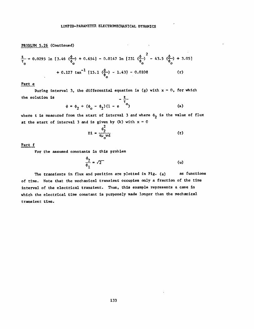
Part f

For the assumed constants in this problem

01

The transients in flux and position are plotted in Fig. (a) as functions

of time. Note that the mechanical transient occupies only a fraction of the time

interval of the electrical transient. Thus, this example represents a case in

which the electrical time constant is purposely made longer than the mechanical

transient time.


Y.iVe0Y\ Av

0,4

0.Z

o o,os oo o 0.20 o.zst/·t. 9.

MIT OpenCourseWare · MIT OpenCourseWare Solutions Manual for Electromechanical Dynamics For any...

Documents

Transcript of MIT OpenCourseWare · MIT OpenCourseWare Solutions Manual for Electromechanical Dynamics For any...