Missing Data under the Matched-Pair Design:

A Practical Guide ∗

Kentaro Fukumoto †

July 17, 2015

∗Paper prepared for delivery at the 32nd Annual Summer Meeting of Society for Political Methodology,Rochester, July 23-25, 2015. Earlier versions, whose title was “Blocking Reduces, if not Removes, AttritionBias,” were presented at the Workshop on Directional Statistics, the Institute of Statistical Mathematics,Tokyo, July 5, 2012, the Symposium on Incomplete Data Analysis and Causal Inference, Osaka University,September 22-23, 2013 and the 1st Asian Political Methodology Meeting, Tokyo Institute of Technology,January 6-7, 2014, the Annual Meeting of the Midwest Political Science Association, Chicago, April 16-19,2015, and workshops at Dartmouth, UCSD, and Washington University in St. Louis. I appreciate commentsfrom Raymond Duch, Jeff Gill, Donald Green, Yusaku Horiuchi, Kosuke Imai, Luke Keele, Gary King, DeanLacy, Ryan T. Moore, Brendan Nyhan, Keith Schnakenberg, and Susumu Shikano. The usual disclaimerapplies.†Professor, Department of Political Science, Faculty of Law, Gakushuin Univer-

sity, 1-5-1 Mejiro, Toshima, Tokyo 171-8588 Japan. Tel: +81-3-3986-0221 ext.4913. Fax: +81-3-5992-1006. Email: Kentaro.Fukumoto@gakushuin.ac.jp. URL:http://www-cc.gakushuin.ac.jp/~e982440/index e.htm.

1

Abstract

The matched-pair design in experiments and matching in observational studies are

powerful tools that enable robust causal inference. What if outcomes of some units

are missing? First, deleting units with missing will lead to bias. Second, some scholars

recommend deleting the other unit in the pair, while others argue that it also results in

biased estimates if missing is not independent of potential outcomes. Third, imputation

is problematic unless missing is at random. By using the potential outcome framework,

this study formalizes estimation error and bias of each method, and establishes that,

when the design and implementation of research is sufficiently good, blockwise deletion

is better than others. This argument is supported by application of these methods to

experimental data of the Mexican universal health insurance program (King et al.,

2007) and non-experimental matched data of training programs (Dehejia and Wahba,

1999; Lalonde, 1986). This paper also shows that the single imputation method is

equivalent to blockwise deletion.

2

INTRODUCTION

The matched-pair design in experiments (Imai, King, and Nall, 2009a; Moore, 2012; Paluck

and Green, 2009) and matching in observational studies (Ho et al., 2007) are powerful tools

to enable pretreatment balance and, therefore, robust causal inference of average treatment

effects (hereafter, ATEs) on an outcome. In the matched-pair design, experimenters make

pairs (or blocks) of two units, each of which shares the exact or simiar values of some

matched-on variables, and randomize treatment assignment within each pair (“block what

you can and randomize what you cannot” (Box, Hunter, and Hunter, 1978, 103). This paper

uses the words “pair” and “block” exchangeably). Or, in the case of observational studies,

analysts match pairs of treated and controlled units so that their covariates are as similar as

possible within each pair and discard non-matched units. In either case, the difference-in-

means of outcomes between the treated and controlled groups estimates the ATE without

bias.

Unfortunately, however, outcome values of units are sometimes missing. This problem

arises more frequently than generally acknowledged. For instance, in the case of randomized

controlled trial, subjects may die, be tired of responding to follow-up survey (Enos, 2014), or

be interrupted politically (King et al., 2007) or elections are uncontested (Panagopoulos and

Green, 2008). When it comes to observational study, examples are that legislators retire, or

duration such as political career is censored (Fukumoto and Masuyama, 2015).

The first, but naive, approach to missing data is the unitwise deletion estimator, that is,

to delete missing observations alone and apply the difference-in-means estimator to all the

remaining units to estmate the ATE. An application example is Panagopoulos and Green

(2008). It is, however, well known that the unitwise deletion estimator can be biased unless

missing is (completely) at random (e.g. Honaker, King, and Blackwell, 2012).

The second, textbook tool to address attrition is the blockwise deletion estimator, which

deletes missing units as well as the other units in the same pairs (namely, blocks) and

calculate difference-in-means by using units in the remaining blocks only (Donner and Klar,

3

2000, 40, Imai, King, and Nall, 2009a, 44, Moore, 2010). Application examples are Enos

(2014) and Family Heart Study Group (1994). It is true that blockwise deletion protects

balance of matched-on variables which would result without missing outcomes, though it is

not sufficient to guarantee unbiased estimation of the ATE. Rather, as Gerber and Green

(2012) warn and this paper also formalizes, the blockwise deletion estimator can “lead[s] to

bias when attrition is a function of potential outcomes” (p. 243). Though King et al. (2007)

argue that the blockwise deletion estimator is unbiased as long as units are missing “for a

reason related to one or more of the variables we matched on” (p. 490), this paper shows that

this statement does not necessarily hold in the presence of heterogeneous treatment effects.

In addition, while Imai, King, and Nall (2009a) claim that the blockwise deletion estimator

“retain[s] the benefits of randomization ... regardless of the missing data mechanism” (p. 44),

this paper demonstrates that the missing data mechanism matters for how much biased the

blockwise deletion estimator is.

The third, general fix for unobserved outcome is the imputation estimators. There are

two variants. On the one hand, the single imputation estimator imputes one value for every

missing outcome by OLS and derives the difference-in-means using both observed and im-

puted outcomes (Giesbrecht and Gumpertz, 2004, 102, Hinkelmann and Kempthorne, 1994,

265-271,Yates, 1933=1970. Details will be explained later). In fact, this paper shows that, in

the matched-pair design, the single imputation estimator is equivalent to the blockwise dele-

tion estmator. On the other hand, the multiple imputation estimator imputes several values

for each missing outcome, calculates the differences-in-means for each imputed datasets, and

uses their average as the estimate of the ATE. There are some methods to impute missing

outcomes, while this paper focuses on Amelia II (Honaker, King, and Blackwell, 2012). Here

is a caveat, though. Multiple imputation assumes “that the data are missing at random ...

that the pattern of missingness only depends on the observed data ... not the unobserved

data” (Honaker, King, and Blackwell, 2012, 4, emphasis added). This assumption is violated

when attrition is a function of potential outcomes. Therefore, imputation of missing values

4

does not necessarily promise solution to attrition bias.

To sum, all the three estimators scholars have uses – unitwise deletion, blockwise dele-

tion, and multiple imputation – can be biased in the presence of missing outcome.1 Which

estimator should we use, practically? Previous works do not examine, much less compare,

the degree to which these estimators suffer from attrition bias. By employing the potential

outcome framework, this paper formalizes estimation error and bias of the unitwise deletion

and blockwise deletion estimators in various conditions. This study also applies the three

estimators to experimental data of the Mexican universal health insurance program (King

et al., 2007) and observational data of training programs (Dehejia and Wahba, 1999; Lalonde,

1986). In a nutshell, the message of this paper is that the blockwise deletion estimator is

better than others as long as the design achieves balance of covariates sufficiently and treat-

ment effect is not so heterogeneous. Moreover, though King et al. (2007, 490) argue that

“whether we delete or impute” does not matter for balance of covariates, this paper shows

that it does matter for estimation of the ATE.

The plan of the paper is as follows. The next section formalizes estimators, lays out

the potential outcome framework, and characterises estimation error and bias of estimators

under some scenarios. The following section demonstrates two applications. The final section

concludes.

FORMAL ANALYSIS

The matched-pair design of either experiments or observational studies is formalized as

follows. Suppose that there are b blocks and each block is composed of two units. Let Yb,u

denote the outcome of unit u ∈ {1, 2} in block b ∈ {1, 2, . . . , b} (which is called unit (b, u)).

Moreover, let Rb,u denote the response of unit (b, u). Rb,u is equal to 1 if Yb,u is observed,

and 0 if Yb,u is missing. Finally, let Tb,u denote the treatment status of unit (b, u). Tb,u is

1If a block is composed of more than two units and has at least one treated unit and one controlled unitobserved, inverse probability weighting is also avialable (Gerber and Green, 2012, 222).

5

equal to 1 if unit (b, u) is assigned and recieves treatment, and 0 otherwise.2 For every block

b, it holds that either Tb,1 = 1, Tb,2 = 0 or Tb,1 = 0, Tb,2 = 1. At this moment, we have not

yet assumed that treatment is randomly assigned. 3

Estimators

Let Wb,u denote genetic weight dummy variable of unit (b, u). Weighted mean of outcome is

calculated as:

E(W ◦ Y ) ≡∑b

b=1

∑2u=1Wb,uYb,u∑b

b=1

∑2u=1Wb,u

.

where, for genetic variable Vb,u, its vector is defined as V ≡ (V1,1, V1,2, V2,1, V2,2, . . . , Vb,1, Vb,2)

and we assume that∑b

b=1

∑2u=1 Wb,u 6= 0. A genetic estimator of the ATE (which we will

define formally in the next subsection) is defined as difference in weighted means:

τ ≡ E(W T ◦ Y )− E(WC ◦ Y ).

It is easy to see that W Tb,u and WC

b,u indicate whether unit (b, u) is counted for calculating

the average of outcomes for treated and controlled groups, respectively. Below, different

estimators have different weights.

If no unit is missing, the full sample estimator is available;

τF ≡ E(W TF ◦ Y )− E(WC

F ◦ Y )

W TF,b,u ≡ Tb,u,

WCF,b,u ≡ 1− Tb,u.

2This paper assumes that all units comply treatment assignment.3If we assume that treatment is randomly assigned, this setup is random allocation of treatment in each

block and is not complete randomization (Moore, 2012), where Tb,u⊥⊥Tb′,u′ unless b = b′ and u = u′, and itis possible that Tb,1 = 1, Tb,2 = 1 or Tb,1 = 0, Tb,2 = 0.

6

The unitwise deletion estimator is defined as

τU ≡ E(W TU ◦ Y )− E(WC

U ◦ Y )

W TU,b,u ≡ Rb,uTb,u,

WCU,b,u ≡ Rb,u(1− Tb,u).

The blockwise deletion estimator is defined as

τB ≡ E(W TB ◦ Y )− E(WC

B ◦ Y )

W TB,b,u ≡ Rb,uRb,−uTb,u,

WCB,b,u ≡ Rb,uRb,−u(1− Tb,u).

The multiple imputation estimator is defined as

τMI ≡1

5

5∑i=1

[E(W TF ◦ Y (i))− E(WC

F ◦ Y (i))],

where Y (i) is the i-th imputed data of Y by Amelia II. Note that the weights are the same

as those of the full sample estimator.

The single imputation estimator is defined as

τSI ≡ E(W TF ◦ Y (S))− E(WC

F ◦ Y (S)),

where Y (S) is the imputed data of Y by the classic method of Hinkelmann and Kempthorne

(1994, 67-72, 265-271). Briefly, it is introduced here (for details, see Appendix). Rearrange

the order of (b, u) so that Yb,u of the first L units, YR=1, are observed and Yb,u of the next M

units, YR=0, are missing (L+M = 2b). Let X the 2b× (b+ 1) design matrix such that, for

7

k ≤ b,

X(b,u),k =

1 if b = k

0 otherwise

and

X(b,u),b+1 = Tb,u,

where X(b,u),k denotes the element of X in the row of unit u of block b and the k-th column.

Let matrices U , V and W such that

(I2b −X(X ′X)−1X ′) =

UL×L VL×M

V ′M×L WM×M

,

where IK is the K ×K identity matrix. Then, in the spirit of OLS, the missing values are

imputed by

YR=0 = −W−1V ′YR=1

and the imputed outcomes are Y (S) = (YR=1, YR=0).

To my knowledge, this paper establishes the following theorem for the first time (all

proofs are in Appendix).

Theorem 1 Equivalence between the single imputation estimator and the blockwise deletion

estimator.

τSI = τB

Thus, we do not have to examine the single imputation estimator, if we do the blockwise

deletion estimator. This theorem also gives another rationale of the blockwise deletion

estimator. Moreover, if two units of the same block become missing at the same time

(Rb,1 = Rb,2 = 0), W is not invertible and, thus, the single imputation estimator does not

work but the blockwise deletion estimator does. Therefore, practitioners only have to employ

8

the blockwise deletion estimator instead of the single imputation estimator.

Needless to say, if no unit has missing outcome, all estimators are reduced to the full

sample estimator because, for all b and u, Rb,u = 1 and Y (i) = Y (S) = Y .

Potential Outcome and Response

The conventional stable unit treatment value assumption (SUTVA) is made. Let Yb,u(1)

and Yb,u(0) denote potential outcomes of unit (b, u) in the case of treatment and control

received, respectively. The realized (but not necessarily observed) outcome can be expressed

as Yb,u = Tb,uYb,u(1) + (1− Tb,u)Yb,u(0). The estimand, the ATE, can be defined in the same

formula as estimators;

τ ≡ E(W TP ◦ Y (1))− E(WC

P ◦ Y (0))

W TP,b,u ≡ 1,

WCP,b,u ≡ 1.

This paper decomposes potential outcomes into six parts;

Yb,u(t) = α + (τ + ∆Bb τ + ∆W

b,uτ)t+ ∆Bb ε+ ∆W

b,uε

provided thatb∑

b=1

∆Bb τ =

2∑u=1

∆Wb,uτ =

b∑b=1

∆Bb ε =

2∑u=1

∆Wb,uε = 0,

where t ∈ {0, 1} (for details, see Appendix). This decomposition is unique. This paper

refers to α as the average of control potential outcomes, ∆Bb ε as between-block error, ∆W

b,uε

as within-block error, ∆Bb τ as between-block heterogeneity of treatment effects, and ∆W

b,uτ

as within-block heterogeneity of treatment effects.

In addition to standard potential outcomes, this paper formalizes missing in the same

framework. Let Rb,u(1) and Rb,u(0) denote potential responses of unit (b, u) in the case of

9

treatment and control received, respectively.4 Rb,u(1) is equal to 1 if Yb,u = Yb,u(1) would be

observed, and 0 if Yb,u = Yb,u(1) would be missing, in the case of treatment received. Rb,u(0)

is equal to 1 if Yb,u = Yb,u(0) would be observed, and 0 if Yb,u = Yb,u(0) would be missing, in

the case of control received. Rb,u(1) and Rb,u(0) are fixed as Yb,u(1) and Yb,u(0) are (Tb,u are

stochastic). The realized reponse can be rewritten as Rb,u = Tb,uRb,u(1) + (1− Tb,u)Rb,u(0).

Below, this paper examines and compares estimation error (in the next subsection) and

bias (in the following subsection) of the unitwise deletion, blockwise deletion, and, as a

reference, full sample estimators.5

Estimation Error

Denote the estimation error of a genetic estimator τ by ∆τ ≡ τU − τ . We have the following

proposition.

Proposition 1 (Estimation Error)

∆τU =E(W TU ◦ (∆Bε+ ∆W ε+ ∆Bτ + ∆W τ))− E(WC

U ◦ (∆Bε+ ∆W ε))

∆τB =E(W TB ◦ (2∆W ε+ ∆Bτ + ∆W τ))

∆τF =E(W TF ◦ (2∆W ε+ ∆W τ)).

To put another way, τB is free of ∆Bε, while τF is free of ∆Bε and ∆Bτ . This paper

emphasizes that, unlike bias, Proposition 1 holds in any one trial without any assumption

on treatment assignment (such as randomness). A caveat is that the order of the estimation

error size among the three estimators, |∆τ |, depends.

When ∆Wb,uε = ∆W

b,uτ = 0, this paper calls the matched-pair design “perfect.” The reason

is that the realized outcome of one unit is the counter-factual of the other unit in the same

4 For this notation, see, for instance, Frangakis and Rubin (1999), Gerber and Green (2012, ch. 7), andMorton and Williams (2010, 182-192).

5This subsection does not consider the multiple imputation estimator because its property depends oncovariates Amelia II employs.

10

pair:

Yb,1(0) = Yb,2(0) = α + ∆Bb ε

Yb,1(1) = Yb,2(1) = α + ∆Bb ε+ τ + ∆B

b τ.

Corollary 1 is easily derived by substituting ∆Wb,uε = ∆W

b,uτ = 0 in Proposition 1.

Corollary 1 (Estimation Error under Perfect Matched-Pair Design) When ∆Wb,uε =

∆Wb,uτ = 0,

∆τU =E(W TU ◦ (∆Bε+ ∆Bτ))− E(WC

U ◦∆Bε)

∆τB =E(W TB ◦∆Bτ)

∆τF =0.

When the matched-pair design is perfect, usually due to covariate balance, the estimation

errors are free of within-block factors, ∆W ≡ {∆W ε,∆W τ}. Note that the full sample

estimator is free of estimation error. Moreover, even if the matched-pair design is not perfect

but nearly so, namely, if ∆Wb,uε and ∆W

b,uτ are sufficiently small (compared to ∆Bb,uε and ∆B

b,uτ),

the estimation errors are almost free of within-block factors and the estimation error size

of τF is more likely to be smaller than those of τB and τU . By contrast, if a matched-pair

design does not succeed in covariates balance and is far from perfect, it would not be helpful

anyway even without missing values (∆τF in Proposition 1).

In addition to ∆Wb,uτ = 0, if ∆B

b,uτ = 0, the treatment effects are homogeneous in the

sense that Yb,u(1) − Yb,u(0) = τ for all (b, u). Corollary 2 is easily derived by substituting

∆Bb,uτ = 0 in Corollary 1.

Corollary 2 Estimation Error under Perfect Matched-Pair Design with Homogeneous Treat-

11

ment Effects. When ∆Wb,uε = ∆W

b,uτ = ∆Bb,uτ = 0,

∆τU =E(W TU ◦∆Bε)− E(WC

U ◦∆Bε)

∆τB =0

∆τF =0.

In this case, not only the full sample estimator but also the blockwise deletion estimator is

free of estimation error. Moreover, even if the treatment effects are not homogeneous but

nearly so, namely, if ∆Bb,uτ is sufficiently small (relative to ∆B

b,uε), the estimation errors are

almost free of between-block heterogeneity of treatment effects, and it is more likely that

|τF | < |τU | and |τB| < |τU |.

Note that perfect matched-pair design is a matter of design, while homogeneous treatment

effects is a matter of implementation. On the one hand, researchers can approach perfect

matched-pair design by improving covariate balance between units within block. On the

other hand, analysts may achieve homogeneous treatment effects by assigning treatment in

as similar a way among units and blocks as possible. However, the latter has already been

implied by SUTVA and the remaining between-block heterogeneity of treatment effects is a

matter of nature and out of control of scholars. By trying to make the matched-pair design

as perfect as possible, designers manage to sort heterogeneity of treatment effects into not

within-block heterogeneity ∆W τ but between-block heterogeneity ∆Bτ . Therefore, unless

total heterogeneity of treatment effects decreases, between-block heterogeneity is unavoidable

even under a perfect matched-pair design. In this sense, between-block heterogeneity is more

severe than covariate balance.

Bias

General Case. Now, this paper assumes ignorability of treatment assignment

(Yb,1(0), Yb,1(1), Yb,2(0), Yb,2(1))⊥⊥(Tb,1, Tb,2)

12

and equal probability of treatment assignment

Pr(Tb,1 = 1, Tb,2 = 0) = Pr(Tb,1 = 0, Tb,2 = 1) =1

2.

Denote bias of genetic estimator τ by ∆τ ≡ E(∆τ) where expectation operator E is taken

over random allocation of T : E(f(T )) ≡∑

T∈{(0,1),(1,0)}b f(T ) Pr(T ) for a genetic function

f(·) of T .6 We assume neither perfect matched-pair design nor homogeneous treatment

effects.

Proposition 2 (Bias)

∆τU =E[E(W TU ◦ (∆Bε+ ∆W ε+ ∆Bτ + ∆W τ))−

E(WCU ◦ (∆Bε+ ∆W ε))]

∆τB =E[E(W TB ◦ (2∆W ε+ ∆Bτ + ∆W τ))]

∆τF =0.

The bias of the full sample estimator is free of within-block factors and zero unlike its

estimation error (Proposition 1). Thus, when we examine biases in special conditions below,

we do not mention ∆τF any more. Let ∆y ∈ {∆Bε,∆W ε,∆Bτ,∆W τ}, WU ∈ {W TU ,W

CU },

and WB ∈ {W TB ,W

CB }. Rough interpretation of E[E(WU ◦∆y)] (or E[E(WB ◦∆y)]) is scaled

covariance between Rb,u (or Rb,uRb,−u) and ∆yb,u. Or, when E[E(W ◦∆y)] = 0, we may say

that W and ∆y are “uncorrelated.”

Proposition 2 does not confirm that the blockwise deletion estimator “retain[s] the ben-

efits of randomization ... regardless of the missing data mechanism” (Imai, King, and

Nall, 2009a, 44); rather, the bias of the blockiwise deletion estimator (∆τB) depends on

relationship between the missing data mechanism (R(0), R(1)) and the potential outcome

∆y, E[E(WB ◦ ∆y)]. In addition, according to King et al. (2007, 490), “if we lose a

6This paper does not assume that treatment assignment is independent between pairs:(Tb,1, Tb,2)⊥⊥(Tb′,1, Tb′,2) for b 6= b′.

13

cluster [i.e. unit] for a reason related to one or more of the variables we matched on

[i.e. E[E(W ◦∆W ε)] = E[E(W ◦∆W τ)] = 0], ... then no bias would be induced for the remain-

ing clusters [i.e. ∆τB = 0].” Nonetheless, according to Proposition 2, if E[E(W TB ◦∆Bτ)] 6= 0,

it can be that ∆τB 6= 0. Thus, existence of ∆Bτ poses difficulty to τB.

Special Cases. When Rb,u(1) = Rb,u(0) = Rb,u, we say the missing data mechanism achieves

“within-unit balance of potential responses.” Good examples are (single or double) blind

test or subliminal stimuli. Since a subject is blind to treatment status (T ), whether the

subject responds or not (R) will not depend on whether treatment is assigned or not (T ).

In this situation, the bias of the blockiwise deletion estimator is free of within-block factors

(E[E(WB ◦ ∆W )] = 0), even if the missing data mechanism is a function of within-block

factors in the sense that E[E(WU ◦∆W )] 6= 0.7

Proposition 3 (Bias Given Within-Unit Balance of Potential Responses) When Rb,u(1) =

Rb,u(0),

∆τU =E[E(W TU ◦ (∆Bε+ ∆W ε+ ∆Bτ + ∆W τ))−

E(WCU ◦ (∆Bε+ ∆W ε))]

∆τB =E[E(W TB ◦∆Bτ)].

When Rb,u(t) = Rb,−u(t), we say the missing data mechanism achieves “within-block

balance of potential responses.” For instance, if matched-on variables (e.g. DNA) completely

explain the missing data mechanism, either two units or no unit in a pair (e.g. twin) should

respond if treatment (or control) is assigned, because two units in a pair share the same (or

similar) value of matched-on variables. Within-block factors (which varies across units in a

block) cannot be responsible for the missing data mechanism (which is the same across units

in a block). In this situation, not only the bias of the blockwise deletion estimator but also

that of the unitwise deletion estimator are free of within-block factors (E[E(W ◦∆W )] = 0).

7In the terminolgy of Gerber and Green (2012, 224-228), in this situation, there are only always-reporters(Rb,u(1) = Rb,u(0) = 1) and never-reporters (Rb,u(1) = Rb,u(0) = 0). The unitwise deletion estimatorprovides an unbiased estimate of the local ATE for always-reporters.

14

Proposition 4 (Bias Given Within-Block Balance of Potential Responses) When Rb,u(t) =

Rb,−u(t),

∆τU =E[E(W TU ◦ (∆Bε+ ∆Bτ))]− E[E(WC

U ◦∆Bε)]

∆τB =E[E(W TB ◦∆Bτ)].

Dunning (2011, 15) denounces blocking, arguing that, for the blockwise deletion estimator

to be unbiased, “we have to assume that all units with the same values of the blocked covari-

ate respond similarly to treatment assignment,” that is, within-block balance of potential

responses. However, even in this condition, the blockwise deletion estimator is still biased,

unless E[E(W TB ◦∆Bτ)] = 0, according to Proposition 4. Or, even if within-block balance of

potential responses does not hold, but if within-unit balance of potential responses (Proposi-

tion 3) or perfect matched-pair design (Corollary 3, see below) is achieved, it follows anyway

that ∆τB = E[E(W TB ◦∆Bτ)].

Under the perfect matched-pair design, bias is simply expectation of estimation error and

∆B is not averaged out. Corollary 3 is easily derived by substituting ∆Wb,uε = ∆W

b,uτ = 0 in

Proposition 2.

Corollary 3 (Bias under Perfect Matched-Pair Design) When ∆Wb,uε = ∆W

b,uτ = 0,

∆τU =E[E(W TU ◦ (∆Bε+ ∆Bτ)]− E[E(WC

U ◦∆Bε)]

∆τB =E[E(W TB ◦∆Bτ)].

Note that Proposition 4 and Corollary 3 lead to the same equations under different condi-

tions. Both are concerned with the design of how to match two units into pairs. If researchers

succeed in balancing all pretreatment variables which decide potential outcomes (Y (1) and

Y (0), Proposition 4) or potential responses (R(1) and R(0), Corollary 3) across units in each

pair by design, E[E(W ◦∆W )] = 0 results. By contrast, Proposition 3 is concerned with not

15

design but implementation of how treatment status (does not) affect(s) potential responses.

If scholars can prevent subjects from knowing treatment status, Proposition 3 is applicable.

In addition, unlike Proposition 4 where within-block balance of potential responses across

units (u = 1, 2) in each block (b) in each treatment status (t) is achieved, Proposition 3 holds

when within-unit balance of potential responses across treatment status (t = 0, 1) in each

unit ((b, u)) is achieved.

Ignorability. Finally, this paper introduces ignorability of unitwise response,8

(Yb,u(0), Yb,u(1))⊥⊥Rb,u

which is equivalent to, given ignorability of treatment assignment,

F (Y (0)|R(0) = 1) = F (Y (0)|R(0) = 0) = F (Y (0))

F (Y (1)|R(1) = 1) = F (Y (1)|R(1) = 0) = F (Y (1)),

where F (·) is the cumulative distribution function. In this condition, E[E(WU ◦ ∆y)] = 0.

Similary, ignorability of blockwise response is defines as

(Yb,u(0), Yb,u(1))⊥⊥Rb,uRb,−u

which is equivalent to, given ignorability of treatment assignment,

F (Yb,u(0)|Rb,u(0)Rb,−u(1) = 1) = F (Yb,u(0)|Rb,u(0)Rb,−u(1) = 0) = F (Yb,u(0))

F (Yb,u(1)|Rb,u(1)Rb,−u(0) = 1) = F (Yb,u(1)|Rb,u(1)Rb,−u(0) = 0) = F (Yb,u(1)),

where F (·) is the cumulative distribution function. In this condition, E[E(WB ◦∆y)] = 0.

Proposition 5 Unbiasedness Given Ignorability of Response.

8Gerber and Green (2012, 229) call this “missing independent of potential outcomes” (MIPO).

16

(1) When (Yb,u(0), Yb,u(1))⊥⊥Rb,u,

∆τU = 0.

(2) When (Yb,u(0), Yb,u(1))⊥⊥Rb,uRb,−u,

∆τB = 0.

Ignorability of unitwise (or blockwise) response is a sufficient, but not a necessary, condition

for unbiasedness of the unitwise (or blockwise) deletion estimator.9

Unfortunately, however, it is unusual that ignorability of response holds. For example,

treated subjects might not feel like showing up in the follow up survey if their outcomes are

not so good in spite of treatment (Rb,u(1) is more likely to be 0 as Y (1) becomes smaller,

and E[E(W T ◦∆y)] is more likely to be larger), while controlled subjects might think they

don’t have to continue experiments if their outcomes are good (Rb,u(0) is more likely to be

0 as Y (0) becomes larger, and E[E(WC ◦∆ε)] is more likely to be smaller). Thus, estimates

of the ATE are expcted be larger than the true ATE (∆τU > 0 and ∆τB > 0).

In Appendix, other special cases where E[E(W ◦ ∆y)] = 0 for some W and ∆y are

introduced.

APPLICATION

The most important message of the previous section is that ∆τB is free from ∆Bε, though ∆τU

is not. The previous section does not characterize properties of ∆τMI analytically because

they depend on behavior of matched-on variables. This section applies these three estima-

tors to real experimental and non-experimental datasets, and compares their performance.10

9Frangakis and Rubin (1999) considers “latent ignorability” where response is ignorable given compliancestatus and monotonicity, and derives an unbiased estimator.

10The previous section does not examine efficiency of estimators. It is difficult to derive their variance

formally because the denominator in∑b

b=1

∑2u=1 Wb,uYb,u∑b

b=1

∑2u=1 Wb,u

varies across trials. Instead, this section considers

variance of estimators by simulation.

17

Though these datasets have no missing value, this paper makes missing values by simulation,

where potential responses (R(1) and R(0)) are functions of ∆Bε only (E[E(WB ◦∆Bε)] 6= 0

and E[E(WU◦∆Bε)] 6= 0), neither ∆W ε nor ∆Bτ nor ∆W τ (E[E(WB◦(∆W ε+∆Bτ+∆W τ))] =

E[E(WU ◦ (∆W ε + ∆Bτ + ∆W τ))] = 0, because the matched-pair design is perfect and

treatment effects are homogeneous). It is not formally clear how ∆τMI behaves, though

missing-at-random assumption (or ignorability of response or MIPO) is violated.11

Experiment

Data. This subsection considers one of the largest randomized field experiments, evaluation of

the universal health insurance program, Segro Popular de Salud (hereafter, SPS), in Mexico

(Imai, 2008; Imai, King, and Nall, 2009a; King et al., 2007, 2009).

A pair of similar areas, which are called “health clusters,” were matched. Treatment (T )

was randomly assigned to either of two clusters in each pair. In a treated cluster, people

were encouraged to sign up SPS, while they were not in a controlled cluster. A resident

of each sampled household in each cluster was interviewed in the baseline survey (at the

time of treatment assignment in August 2005) and the follow-up survey (10 months after the

treatment assignment). The unit of observation is household (the dataset contains 32,515

respondents), though the unit of randomization is cluster (50 pairs of clusters). Thus, this

paper analyzes cluster-level data, as Imai (2008) does.12

Among hundreds of outcomes, previous studies have examined most intensively “catas-

trophic health expenditure,” i.e. out-of-pocket health-care expenditures greater than 30 per-

cent of disposal income. Following Imai (2008, 4868), the outcome this paper studies (Y ) is

the proportion of households suffering catastrophic health expenditure in every cluster.

Indeed, the investigators utilized the matched-pair design exactly because they prepared

11In the previous section, R(0) and R(1) are fixed, while T is random. In this section, R(0) and R(1) arerandom, while T is fixed (Y (0) and Y (1) are fixed in both sections). Therefore, admittedly, both sectionsare not strictly comparable. However, Monte Carlo simulation of this section will give us practiacl sense ofhow each estimator behaves in real setups.

12The data this paper uses is Imai, King, and Nall (2009b). This paper aggregates the original individual-level data into cluster-level data (Imai, 2008, 4868).

18

for missing values. Before they observed outcomes, King et al. (2007, 489, emphasis original)

wrote,

[T]he PROGRESA evaluation ... had some loss of observations ... given this

previous experience, we must expect to lose health clusters, and so we need a

design that allows some clusters to be lost, under at least some circumstances,

without also losing the advantages of randomization. Thus, we turn to what is

known as a randomized cluster matched pair design.

Eventually, no cluster has missing values. Thus, this paper turns some actually observed

outcome values into missing ones by way of the following procedure.

Method. According to the framework of this paper, below, clusters and their pairs are referred

to as “units” and “blocks,” respectively (b = 50). First, the fixed effects of block b, ∆Bb ≡

α+∆Bb ε+∆B

b τ , is estimated by ∆Bb = (yb,1 +yb,2− τF )/2 (note that the full sample estimator

is applicable because no cluster is missing in fact).13 Then, the weight for randomly assigning

missing to unit (b, u) is calculated as ωb,u ≡ Φ(ρ[tb,u∆Bb − (1 − tb,u)∆B

b ]), where Φ(·) is the

cumulative density function of the standard normal distribution. In the case of ρ > 0, the

larger ∆Bb , the more (or less) likely Rb,u(1) (or Rb,u(0)) is to be 0. In the case of ρ < 0, the

opposite holds. Thus, ρ represents direction and strength of the relationship between within-

unit-unbalanced potential responses and between-block factor.14 Denote the proportion of

missing units by m. The values of ρ and m are specified shortly.

Fix the values of ρ and m. For one trial, mb units are chosen randomly from treated and

controlled groups, respectively, following the above weight ωb,u, and their values of Yb,u are

turned into missing. Then, τB and τU are estimated. When τMI is estimated, missing values

are imputed by Amelia II using 17 pretreatment variables and making 5 imputed datasets.15

13The next version of the paper will use ∆Bb ≡ ∆B

b ε + ∆Bb τ , which is estimated by ∆B

b ≡ ((yb,1 + yb,2 −τF )/2)− α, where α ≡ b−1

∑bb=1((yb,1 + yb,2 − τF )/2).

14If we make within-unit-balanced potential response by, say, ωb,u ≡ Φ(ρ∆Bb ), both τU and τB are unbiased

according to Proposition 3 and E[E(WU ◦ (∆W ε+ ∆W τ))] = 0 (though E[E(W ◦ (∆Bε+ ∆Bτ))] 6= 0. Whythis is the case is a future agenda). Since this is not interesting, this paper does not take this strategy.

15For details about 17 matched-on pretreatment variables, see Appendix.

19

In addition, in order to examine what if blocking is not successful, the failing blockwise

deletion estimator, τNB, is also applied. Namely, this paper randomly makes pairs of units

irrespetive of the original block, regard the new pairs as blocks and applies the blockwise

deletion estimator.

This trial is repeated 1,000 times for one set of values of ρ and m. For each estimator,

the average and the 2.5-97.5 percentile range of 1,000 estimates are recorded.

Results. Figure 1 shows the case where ρ varies from −0.9 to 0.9 by 0.1 and m is constantly

equal to 0.1.16 The horizontal axis represents ρ, while the vertical axis indicates τ . The

baseline is the estimate by the full sample estimator, τF = −1.27 (Imai, 2008, 4868), because

no unit is missing actually and τF is available.17

Figure 1: Estimates by Four Estimators of ATE (τ , vertical axis) against Relationship (ρ,horizontal axis) between ∆B

b and Rb,u(t). Missing proportion is m = 0.1. ExperimentalData.

−0.5 0.0 0.5

−2.

5−

2.0

−1.

5−

1.0

−0.

50.

0

Relation b/w Between−Block Error and Treated Missing Probability

Trea

tmen

t Effe

ct

● ● ● ● ● ● ● ● ● ● ● ● ● ● ● ● ● ● ●

The vertical thick lines and big points correspond to the 2.5-97.5 percentile ranges and

16This study uses R Development Core Team (2012) for conducting simulation, analyzing data, anddrawing figures.

17Imai (2008, 4868) reports τF = 1.27, which seems to be simply a typo. The true ATE, τ , is obviouslyunknown.

20

averages of 1,000 estimates by the blockwise deletion estimator, τB, for each value of ρ. It is

easy to see that the points are almost equal to τF , because the missing data mechanism is a

function of ∆B but not ∆W , and ∆τB is free of ∆Bε. 18

The gray area and the thin dotted line represent the 2.5-97.5 percentile ranges and

averages of estimates by the unitwise deletion estimator, τU . The larger the size of |ρ|, the

more τU deviates from τF . The size and direction of the deviation depends on E[E(W TU ◦

∆Bε)] = −E[E(WCU ◦ ∆Bε)], which is managed by ρ. Furthermore, the gray area does not

contain τF for relatively larger values of ρ; thus, the null hypothesis of τ = τF would be

rejected.

The shaded area and the thick dotted line show the 2.5-97.5 percentile ranges and averages

of estimates by the multiple imputation estimator, τMI . The thick dotted line deviates from

τF for most of values of ρ, though to lesser degree than τU . Blockwise deletion makes

most of blocking, while multiple imputation usually cannot use it because the number of

blocks is too large (half of the number of units). When the matched-pair design is (almost)

perfect, pairs can explain more variation in dependent variables than covariates multiple

imputation utilizes can do and, therefore, the blockwise deletion estimator outperforms the

multiple imputation estimator. Recall also that assumption of missing at random is violated.

Fortunately, the shaded area always includes τF .

Finally, the vertical thin lines and small points correspond to the 2.5-97.5 percentile

ranges and averages of estimates by the failing blockwise deletion estimator, τNB. Clearly,

it deviates from τF almost as much as τU . Therefore, when the matched-pair design is far

from perfect, the blockwise deletion estimator does not work well.

Two general remarks are in order. First, when attrition is not a function of potential

outcomes (ρ = 0), the averages of all four estimators convege to τF . Second, a downside

of the blockwise deletion estimator is its larger 2.5-97.5 percentile range relative to those of

other estimators, naturally because τB utilizes smaller number of units than τU and τMI .

18∆B includes ∆Bε and ∆Bτ . One cannot, however, identify ∆Bε and ∆Bτ separately.

21

Figure 2 shows the case where the missing proportion m varies from 0.1 to 0.5 by 0.1

and ρ is constantly equal to 0.5. The horizontal axis represents m, while the vertical axis

indicates τ . The horizontal thin dotted line indicates τF . The estimates of all the four

estimators are displayed in the same way as in Figure 1. Implication of Figure 1 becomes

more severe, as more units are missing (m becomes larger).

Figure 2: Estimates by Four Estimators (τ , vertical axis) against Missing Proportion (m,horizontal axis). ρ = 0.5. Experimental Data.

0.1 0.2 0.3 0.4 0.5

−8

−6

−4

−2

02

Proportion of Missing

Trea

tmen

t Effe

ct

● ● ● ● ●

Observatioal Study

Data. This subsection switches to one of the most famous non-experimental data, which

Dehejia and Wahba (1999) and Lalonde (1986) analyze. Their goal is to estimate the ATE

of a labor training program (T ) in the National Supported Work (NSW) Demonstration on

post-intervention income levels in 1978 (Y ). To that end, Lalonde (1986) constructs a dataset

by combining the experimental treated units from the NSW dataset with non-experimental

controlled units from the Current Population Survey (CPS). Since the NSW and CPS units

are not comparable, Dehejia and Wahba (1999) apply propensity score matching to the subset

22

of the Lalonde’s (1986) original dataset (only those whose earnings in 1974 are available)

so that observed preintervention variables are balanced between the treated and controlled

groups.

This paper applies Sekhon’s (2011) multivariate and propensity score matching algorithm,

Matching package in a statistical environment R, to Dehejia and Wahba’s (1999) dataset.19

Among 185 treated units and 15,992 controlled units, b = 223 matched pairs are coupled. In

the framework of this paper, a pair corresponds to a block.

Method. The simulation procedure is basically the same as that of the previous Mexican

application. Exceptions are as follows. The fixed effects of block b, ∆Bb ≡ ∆B

b ε + ∆Bb τ + τ ,

is estimated by ∆Bb = (yb,1 + yb,2 − α)/2, where α ≡ b−1

∑bb=1((yb,1 + yb,2 − τF )/2). 20 When

τMI is estimated, missing values are imputed by Amelia II using the same nine pretreatment

variables as Matching package uses.21

Results. Figure 3 shows the case where ρ ranges between −0.0009 to 0.0009 by 0.0001 and m

is constantly equal to 0.1. The horizontal axis represents ρ, while the vertical axis indicates

τ . The estimates of all the four estimators are displayed in the same way as in Figure 1. If

no unit is missing, the estimate by the full sample estimator, τF = 1913.2, is available, which

is indicated by the horizontal thin dotted line.22 Implication of the results is the same as

that of the Mexican application. Noticeable difference is that τMI is worse than that in the

previous subsection and is now as bad as τU . It calls attention given that matching algorithm

(Matching, which affects performance of τB) and multiple imputation algorithm (Amelia II,

which affects performance of τMI) take advantage of the same nine pretreatment variables.

Figure 4 shows the case where the missing proportion m varies from 0.1 to 0.5 by 0.1

and ρ is constantly equal to 0.0005. The horizontal axis represents m, while the vertical

axis indicates τ . The estimates of all the four estimators are displayed in the same way

19For details about data and matching procedure, see Appendix.20The next version of the paper will use ∆B

b ≡ ∆Bb ε + ∆B

b τ , which is estimated by ∆Bb = ((yb,1 + yb,2 −

τF )/2)− α.21As for the nine matched-on variables, see Appendix.22The true ATE, τ , is obviously unknown.

23

Figure 3: Estimates by Four Estimators of ATE (τ , vertical axis) against Relationship (ρ,horizontal axis) between ∆B

b and Rb,u(t). Missing proportion is m = 0.1. ObservationalStudy Data.

−5e−04 0e+00 5e−04

500

1000

1500

2000

2500

3000

Relation b/w Between−Block Error and Treated Missing Probability

Ave

rage

Tre

atm

ent E

ffect

● ● ● ● ● ● ● ● ● ● ● ● ● ● ●●

● ● ●

as in Figure 2. The upper and lower horizontal thin dotted lines indicate τF and τ = 0,

respectively. Again, implication of the results is the same as that of the previous Mexican

application. Implication of Figure 3 becomes more severe, as more units are missing (m

becomes larger). In particular, when m ≥ 0.4, the 2.5-97.5 percentile ranges of τU , τMI , and

τNB are below zero; thus, the alternative hypothesis τ < 0 would be supported by these

estimators, even if τF > 0.

CONCLUSION

When the missing data mechanism is not independent of potential outcomes in experiments

with the matched-pair design or observational study with matching, all of the blockwise

deletion, unitwise deletion, single imputation and multiple imputation estimators can be

biased. Balance of pretreatment variables does not guarantee unbiased estimation of the

ATE in the presence of attrition. In practice, however, analysts should choose at least one

24

Figure 4: Estimates by Four Estimators (τ , vertical axis) against Missing Proportion (m,horizontal axis). ρ = 0.0005. Observational Study Data.

0.1 0.2 0.3 0.4 0.5

−40

00−

2000

020

0040

00

Proportion of Missing

Trea

tmen

t Effe

ct● ●

● ●

●

estimator. A practical advice of this paper is simple: use the blockwise deletion estimator.

The reasons are summarized as follows.

1. The blockwise deletion estimator is equivalent to the single imputation estimator (The-

orem 1).

2. The blockwise deletion estimator cancels out between-block error and, thus, reduces a

source of estimation error (Proposition 1), while the unitwise deletion estimator does

not.

3. The blockwise deletion estimator is more likely to have smaller estimation error than

the unitwise deletion estimator, as a matched-pair design succeeds in achieving balance

of more pretreatment variables which decide potential outcome, and treatment effects

are less heteregeneous (Corollary 2).

4. The blockwise deletion estimator is more likely to have smaller bias than the unitwise

deletion estimator, as a matched-pair design succeeds in achieving balance of more

25

pretreatment variables which decide potential response, and treatment effects are less

heteregeneous (Proposition 4).

5. The blockwise deletion estimator is more likely to have smaller bias than the unitwise

deletion estimator, as a researcher can implement treatment assignment with subjects

blind to it more successfully, and treatment effects are less heteregeneous (Proposition

3).

6. The blockwise deletion estimator takes advantage of information about which unit is

paired with which unit, while the multiple imputation estimator cannot. It is difficult

to find such covariates that are as informative as blocks and, thus, enable as good

imputation as the matched-pair design. (as shown in Application)

At the same time, researchers should not forget a caveat that even a perfect matched-pair

design cannot remove attrition bias due to between-block heterogeneity of treatment effects,

which is almost unavoidable (Corollary 3). The main contribution of this paper is to clarify

the findings above by formalizing the relationship between components of potential outcomes

and potential reponses.

The relationship between blocking and attrition bias has attracted less attention than

it should and is complicated enough to need thorough consideration. This work aims to

contribute to this issue, though there remain many research agendas. For instance, this

study focuses on blocks composed of a pair of units, while, in many studies, blocks are

composed of more than two units. In this case, inverse probability weighting (Gerber and

Green, 2012, 222) is available, where weight variable W is not a dummy but a real number

which is not smaller than one. For another example, units sometimes do not comply with

treatment assignment, even if their outcomes are observed. A typical solution is instrumental

variable estimation (Angrist, Imbens, and Rubin, 1996). It is not clear, however, whether

or in what condition the blockwise deletion estimator is better than inverse probability

weighting or instrumental variable estimation. Studying these topics is future agenda.

26

References

Angrist, Joshua D., Guido W. Imbens, and Donald B. Rubin. 1996. “Indentification of Causal

Effects Using Instrumental Variables.” Journal of the American Statistical Association

91(434): 444–455.

Box, George E. P., William G. Hunter, and J. Stuart Hunter. 1978. Statistics for Exper-

imenters: An Introduction to Design, Data Analysis, and Model Building. New York:

Wiley.

Dehejia, Rajeev, and Sadek Wahba. 1999. “Causal Effects in Non-Experimental Studies:

Reevaluating the Evaluation of Training Programs.” Journal of the American Statistical

Association 94(448): 1053–1062.

Donner, Allan, and Neil Klar. 2000. Design and Analysis of Cluster Randomization Trials

in Health Research. London: Arnold.

Dunning, Thad. 2011. “Does Blocking Reduce Attrition Bias?” Experimental Political

Scientist: Newsletter of the APSA Experimental Section 2(1): 12–16.

Enos, Ryan D. 2014. “Causal effect of intergroup contact on exclusionary attitudes.” Pro-

ceedings of the National Academy of Sciences 111(10): 3699–3704.

Family Heart Study Group. 1994. “Randomised Controlled Trial Evaluating Cardiovascular

Screening and Intervention in General Practice: Principal Results of British Family Heart

Study.” British Medical Journal 308(6924): 313–20.

Frangakis, Constantine E., and Donald B. Rubin. 1999. “Addressing Complications

of Intention-to-Treat Analysis in the Combined Presence of All-or-None Treatment-

Noncompliance and Subsequent Missing Outcomes.” Biometrika 86(2): 365–379.

Fukumoto, Kentaro, and Mikitaka Masuyama. 2015. “Measuring Judicial Independence

27

Reconsidered: Survival Analysis, Matching, and Average Treatment Effects.” Japanese

Journal of Political Science 16(1): 33–51.

Gerber, Alan S., and Donald P. Green. 2012. Field Experiments: Design, Analysis, and

Interpretation. New York: W. W. Norton & Company.

Giesbrecht, Francis G., and Marcia L. Gumpertz. 2004. Planning, Construction, and Statis-

tical Analysis of Comparative Experiments. New York: Wiley.

Hinkelmann, Klaus, and Oscar Kempthorne. 1994. Design and Analysis of Experiments.

Volume I: Introduction to Experimental Design. New York: John Wiley and Sons, Inc.

Ho, Daniel, Kosuke Imai, Gary King, and Elizabeth Stuart. 2007. “Matching as Nonpara-

metric Preprocessing for Reducing Model Dependence in Parametric Causal Inference.”

Political Analysis 15: 199–236.

Honaker, James, Gary King, and Matthew Blackwell. 2012. “AMELIA II: A Program for

Missing Data.”.

Imai, Kosuke. 2008. “Variance Identification and Efficiency Analysis in Randomized Exper-

iments under the Matched-Pair Design.” Statistics in Medicine 27(24): 4857–4873.

Imai, Kosuke, Gary King, and Clayton Nall. 2009a. “The Essential Role of Pair Matching

in Cluster-Randomized Experiments, with Application to the Mexican Universal Health

Insurance Evaluation (with discussions and rejoinder).” Statistical Science 24(1): 29–53.

Imai, Kosuke, Gary King, and Clayton Nall. 2009b. “Replication data for: The Essential Role

of Pair Matching in Cluster-Randomized Experiments, with Application to the Mexican

Universal Health Insurance Evaluation.”.

King, Gary, Emmanuela Gakidou, Kosuke Imai, Jason Lakin, Ryan T. Moore, Clayton Nall,

Nirmala Ravishankar, Manett Vargas, Martha Mara Tllez-Rojo, Juan Eugenio Hernndez

vila, Mauricio Hernndez vila, and Hctor Hernndez Llamas. 2009. “Public Policy for the

28

Poor? A Randomised Assessment of the Mexican Universal Health Insurance Programme.”

Lancet 373: 1447–1454.

King, Gary, Emmanuela Gakidou, Nirmala Ravishankar, Ryan T. Moore, Jason Lakin,

Manett Vargas, Martha Mara Tllez-Rojo, Juan Eugenio Hernndez vila, Mauricio Hernndez

vila, and Hctor Hernndez Llamas. 2007. “A “Politically Robust” Experimental Design for

Public Policy Evaluation, with Application to the Mexican Universal Health Insurance

Program.” Journal of Policy Analysis and Management 26: 479–506.

Lalonde, Robert. 1986. “Evaluating the Econometric Evaluations of Training Programs.”

American Economic Review 76: 604–620.

Moore, Ryan T. 2010. “Blocking Political Science Experiments: Why, How, and Then

What?” Experimental Political Scientist: Newsletter of the APSA Experimental Section

1(1): 3–5.

Moore, Ryan T. 2012. “Multivariate Continuous Blocking to Improve Political Science Ex-

periments.” Political Analysis 20(4): 460–479.

Morton, Rebecca B., and Kenneth C. Williams. 2010. Experimental Political Science and

the Study of Causality: From Nature to the Lab. Cambridge: Cambridge University Press.

Paluck, Elizabeth Levy, and Donald P. Green. 2009. “Deference, Dissent, and Dispute Reso-

lution: An Experimental Intervention Using Mass Media to Change Norms and Behavior

in Rwanda.” American Political Science Review 103(4): 622–644.

Panagopoulos, Costas, and Donald P Green. 2008. “Field experiments testing the impact

of radio advertisements on electoral competition.” American Journal of Political Science

52(1): 156–168.

R Development Core Team. 2012. “R: A Language and Environment for Statistical Com-

puting.”.

29

Sekhon, Jasjeet S. 2011. “Multivariate and Propensity Score Matching Software with Auto-

mated Balance Optimization: The Matching package for R.” Journal of Statistical Software

42(7): 1–52.

Yates, Frank. 1933=1970. The Analysis of Replicated Experiments When the Field Results

Are Incomplete. London: Griffin pp. 41–56.

30

APPENDIX

Single Imputation

Definition. The single imputation method explained by Hinkelmann and Kempthorne (1994,

67-72, 265-271) is as follows. Let (b, T ) = (b, 1) and (b, C) = (b, 2) if Tb,1 = 1 and (b, T ) =

(b, 2) and (b, C) = (b, 1) if Tb,2 = 1. Note that Rb,T = Rb,1Tb,1 + Rb,2Tb,2 and Rb,C =

Rb,1(1 − Tb,1) + Rb,2(1 − Tb,2). Suppose that two units of the same block never become

missing at the same time and rearrange block number b so that

{b|Rb,T = 1, Rb,C = 1} ≡ BL = {1, . . . , L}

{b|Rb,T = 1, Rb,C = 0} ≡ BT = {L+ 1, . . . , L+MT}

{b|Rb,T = 0, Rb,C = 1} ≡ BC = {L+MT + 1, . . . , L+MT +MC}

{b|Rb,T (1) = 0, Rb,C(0) = 0} = ∅

∴ L+MT +MC = b = N/2.

Let Y ∗ such that

Y ∗b,u = Yb,u if Rb,u = 1

Y ∗b,u = 0 if Rb,u = 0.

Make the following model:

Y ∗ = Xβ + ZYR=0 + ε

β = (β1, β2, . . . , βb, τ)

βb = α + ∆Bb ε

εb,u = ∆Wb,uε+ (∆B

b τ + ∆Wb,uτ)Tb,u

YR=0 = (YL+1,C , YL+2,C , . . . , YL+MT ,C , YL+MT +1,T , YL+MT +2,T , . . . , YL+MT +MC ,T )

31

where X is the design matrix

X =

I(b = 1) · · · I(b = b) Tb,u

(b ∈ BL, T ) IL 0L×MT 0L×MC 1L×1

(b ∈ BL, C) IL 0L×MT 0L×MC 0L×1

(b ∈ BT , T ) 0MT×L IMT 0MT×MC 1MT×1

(b ∈ BC , C) 0MC×L 0MC×MT IMC 0MC×1

(b ∈ BT , C) 0MT×L IMT 0MT×MC 0MT×1

(b ∈ BC , T ) 0MC×L 0MC×MT IMC 1MC×1

,

and Z is the missing indicator matrix

Z =

I(b = L+ 1) I(b = b)

(b ∈ BL, T ) 0L×MT 0L×MC

(b ∈ BL, C) 0L×MT 0L×MC

(b ∈ BT , T ) 0MT×MT 0MT×MC

(b ∈ BC , C) 0MC×MT 0MC×MC

(b ∈ BT , C) −IMT 0MT×MC

(b ∈ BC , T ) 0MC×MT −IMC

,

where IK is the K ×K identity matrix, 0K1×K2 is the K1 ×K2 matrix whose elements are

all zero, and 1K1×K2 is the K1 ×K2 matrix whose elements are all one. Let matrices U , V

and W such that

(IN −X(X ′X)−1X ′) =

U(2L+MT +MC)×(2L+MT +MC) V(2L+MT +MC)×(MT +MC)

V ′(MT +MC)×(2L+MT +MC) W(MT +MC)×(MT +MC)

.

By OLS (namely, minimizing∑ε2), it follows

YR=0 = −W−1V ′YR=1,

32

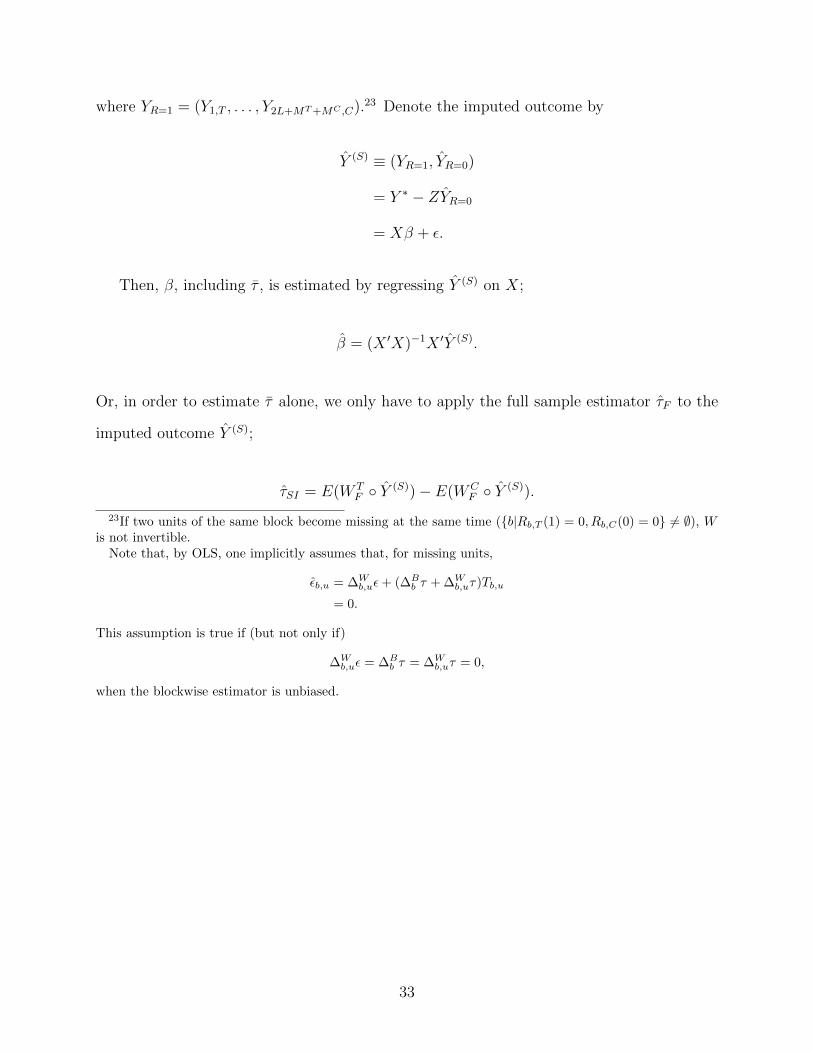
where YR=1 = (Y1,T , . . . , Y2L+MT +MC ,C).23 Denote the imputed outcome by

Y (S) ≡ (YR=1, YR=0)

= Y ∗ − ZYR=0

= Xβ + ε.

Then, β, including τ , is estimated by regressing Y (S) on X;

β = (X ′X)−1X ′Y (S).

Or, in order to estimate τ alone, we only have to apply the full sample estimator τF to the

imputed outcome Y (S);

τSI = E(W TF ◦ Y (S))− E(WC

F ◦ Y (S)).

23If two units of the same block become missing at the same time ({b|Rb,T (1) = 0, Rb,C(0) = 0} 6= ∅), Wis not invertible.

Note that, by OLS, one implicitly assumes that, for missing units,

εb,u = ∆Wb,uε+ (∆B

b τ + ∆Wb,uτ)Tb,u

= 0.

This assumption is true if (but not only if)

∆Wb,uε = ∆B

b τ = ∆Wb,uτ = 0,

when the blockwise estimator is unbiased.

33

Proof of Theorem 1. The variance covariance matrix of the design matrix is

X ′X =

b1 b2 · · · bb Tb,u

b1 2 0 · · · 0 1

b2 0 2 · · · 0 1

......

.... . .

......

bb 0 0 · · · 2 1

Tb,u 1 1 · · · 1 b

.

Its inverse is

(X ′X)−1 =

b1 b2 · · · bb Tb,u

b1 2−1 +N−1 N−1 · · · N−1 −2N−1

b2 N−1 2−1 +N−1 · · · N−1 −2N−1

......

.... . .

......

bb N−1 N−1 · · · 2−1 +N−1 −2N−1

Tb,u −2N−1 −2N−1 · · · −2N−1 4N−1

.

The projection matrix is

X(X ′X)−1X ′ =

(BL, T ) BL, C) (BT , T ) (BC , C) (BT , C) (BC , T )

(BL, T ) SsL×L SdL×L DsL×MT DdL×MC DdL×MT DsL×MC

(BL, C) SdL×L SsL×L DdL×MT DsL×MC DsL×MT DdL×MC

(BT , T ) DsMT×L DdMT×L SsMT×MT DdMT×MC SdMT×MT DsMT×MC

(BC , C) DdMC×L DsMC×L DdMC×MT SsMC×MC DsMC×MT SdMC×MC

(BT , C) DdMT×L DsMT×L SdMT×MT DsMT×MC SsMT×MT DdMT×MC

(BC , T ) DsMC×L DdMC×L DsMC×MT SdMC×MC DdMC×MT SsMC×MC

,

34

where the K ×K design covariance matrix of the Same block group and same assignment is

SsK×K =

2−1 +N−1 N−1 · · · N−1

N−1 2−1 +N−1 · · · N−1

......

. . ....

N−1 N−1 · · · 2−1 +N−1

,

the K ×K design covariance matrix of the Same block group and different assignment is

SdK×K =

2−1 −N−1 −N−1 · · · −N−1

−N−1 2−1 −N−1 · · · −N−1

......

. . ....

−N−1 −N−1 · · · 2−1 −N−1

,

the K1 ×K2 design covariance matrix of Different block groups and same assignment is

DsK1×K2 =

N−1 N−1 · · · N−1

N−1 N−1 · · · N−1

......

. . ....

N−1 N−1 · · · N−1

,

and the K1×K2 design covariance matrix of Different block groups and different assignment

is

DdK1×K2 =

−N−1 −N−1 · · · −N−1

−N−1 −N−1 · · · −N−1

......

. . ....

−N−1 −N−1 · · · −N−1

.

35

It follows

V =

(BT , C) (BC , T )

(b ∈ BL, T ) −DdL×MT −DsL×MC

(b ∈ BL, C) −DsL×MT −DdL×MC

(b ∈ BT , T ) −SdMT×MT −DsMT×MC

(b ∈ BC , C) −DsMC×MT −SdMC×MC

W =

(BT , C) (BC , T )

(b ∈ BT , C) IMT×MT − SsMT×MT −DdMT×MC

(b ∈ BC , T ) −DdMC×MT IMC×MC − SsMC×MC

W−1 =

(BT , C) (BC , T )

(b ∈ BT , C) SMT×MT DMT×MC

(b ∈ BC , T ) DMC×MT SMC×MC

,where

SK×K =

2 + 2L−1 2L−1 · · · 2L−1

2L−1 2 + 2L−1 · · · 2L−1

......

. . ....

2L−1 2L−1 · · · 2 + 2L−1

DK1×K2 =

−2L−1 −2L−1 · · · −2L−1

−2L−1 −2L−1 · · · −2L−1

......

. . ....

−2L−1 −2L−1 · · · −2L−1

.

We have

V ′YR=1 =

(BT , T ) 1N

(∑b∈BL∪BT Yb,T −

∑b∈BL∪BC Yb,C

)− 1

2YBT ,T

(BC , C) − 1N

(∑b∈BL∪BT Yb,T −

∑b∈BL∪BC Yb,C

)− 1

2YBC ,C

.36

Since

−W−1V ′YR=1 = YR=0

τB =1

L

(∑b∈BL

Yb,T −∑b∈BL

Yb,C

),

the imputed outcomes are

Yb∈BT ,C = Yb,T −[( 2

N+

2(MT +MC)

NL

)( ∑b∈BL∪BT

Yb,T −∑

b∈BL∪BCYb,C

)− 1

L(∑b∈BT

Yb,T −∑b∈BC

Yb,C)]

= Yb,T − τB

Yb∈BC ,T = Yb,C +[( 2

N+

2(MT +MC)

NL

)( ∑b∈BL∪BT

Yb,T −∑

b∈BL∪BCYb,C

)− 1

L(∑b∈BT

Yb,T −∑b∈BC

Yb,C)]

= Yb,C + τB.

Therefore,

τSI = E(W TF ◦ Y (S))− E(WC

F ◦ Y (S))

= b−1

b∑b=1

(Yb,T − Yb,C)

=1

L

∑b∈BL

(Yb,T − Yb,C) +1

MT

∑b∈BT

(Yb,T − Yb,C) +1

MC

∑b∈BC

(Yb,T − Yb,C)

= τB +1

MT

∑b∈BT

τB +1

MC

∑b∈BC

τB

= τB.�

Unique Decomposition of Potential Outcome

The ATE is calculated as

τ ≡ E(W TP ◦ Y )− E(WC

P ◦ Y )

=

∑2b=1

∑2u=1W

TP,b,uYb,u(1)∑2

b=1

∑2u=1 W

TP,b,u

−∑2

b=1

∑2u=1W

CP,b,uYb,u(0)∑2

b=1

∑2u=1W

CP,b,u

.

37

The block treatment effect of block b is defined as

τb ≡∑2

u=1 WTP,b,uYb,u(1)∑2

u=1WTP,b,u

−∑2

u=1 WCP,b,uYb,u(0)∑2

u=1WCP,b,u

.

The unit treatment effect of unit (b, u) is defined as

τb,u ≡W T

P,b,uYb,u(1)

W TP,b,u

−WC

P,b,uYb,u(0)

WCP,b,u

.

Between-block heterogeneity of treatment effect of block b is derived by

∆Bb τ = τb − τ .

Within-block heterogeneity of treatment effect of unit (b, u) is derived by

∆Wb,uτ = τb,u − τb.

The average of control potential outcomes is derived by

α ≡ E(WCP ◦ Y )

=

∑2b=1

∑2u=1W

CP,b,uYb,u(0)∑2

b=1

∑2u=1 W

CP,b,u

.

The average of control potential outcomes of block b is defined as

αb ≡∑2

u=1 WCP,b,uYb,u(0)∑2

u=1WCP,b,u

.

Between-block error of block b is derived by

∆Bb ε = αb − α.

38

Within-block error of unit (b, u) is derived by

∆Wb,uε = Yb,u(0)− αb.

Sketch of Proof

Proposition 1. Before we prove Proposition 1, we prove the following two lemmas.

Lemma 1

E(W ◦ (∆y + ∆y′)) = E(W ◦∆y) + E(W ◦∆y′)

Proof

E(W ◦ (∆y + ∆y′)) =

∑bb=1

∑2u=1Wb,u(∆y + ∆y′)∑bb=1

∑2u=1 Wb,u

=

(∑bb=1

∑2u=1 Wb,u∆y

)+(∑b

b=1

∑2u=1Wb,u∆y′

)∑b

b=1

∑2u=1Wb,u

= E(W ◦∆y) + E(W ◦∆y′)

�

Lemma 2

∆τ =E(W T ◦ (∆Bε+ ∆W ε+ ∆Bτ + ∆W τ))−

E(WC ◦ (∆Bε+ ∆W ε)).

Proof Note that T 2b,u = Tb,u, (1 − Tb,u)2 = 1 − Tb,u and Tb,u(1 − Tb,u) = 0. It follows that

W Tb,uTb,u = W T

b,u,WCb,u(1− Tb,u) = WC

b,u, and W Tb,u(1− Tb,u) = WC

b,uTb,u = 0. Thus, by Lemma

39

1,

E(W T ◦ Y ) = E(W T ◦ (T (1)Y (1) + (1− T (1))Y (0)))

= E(W T ◦ Y (1))

E(WC ◦ Y ) = E(W T ◦ (T (1)Y (1) + (1− T (1))Y (0)))

= E(WC ◦ Y (0))

By Lemma 1,

τ − τ =E(W T ◦ Y )− E(WC ◦ Y )− τ

=E(W T ◦ Y (1))− E(WC ◦ Y (0))− τ

=E(W T ◦ (α + ∆Bε+ ∆W ε+ τ + ∆Bτ + ∆W τ))

− E(WC ◦ (α + ∆Bε+ ∆W ε))− τ

=E(W T ◦ α) + E(W T ◦ τ) + E(W T ◦ (∆Bε+ ∆W ε+ ∆Bτ + ∆W τ))

− E(WC ◦ α)− E(WC ◦ (∆Bε+ ∆W ε))− τ

=α + τ + E(W T ◦ (∆Bε+ ∆W ε+ ∆Bτ + ∆W τ))

− α− E(WC ◦ (∆Bε+ ∆W ε))− τ

=E(W T ◦ (∆Bε+ ∆W ε+ ∆Bτ + ∆W τ))

− E(WC ◦ (∆Bε+ ∆W ε)).

�

40

Note that

2∑u=1

W TB,b,u∆W

b,uε =2∑

u=1

Rb,u(1)Rb,−u(0)Tb,u∆Wb,uε

=2∑

−u=1

Rb,−u(1)Rb,u(0)Tb,−u∆Wb,−uε

=2∑

−u=1

Rb,u(0)Rb,−u(1)(1− Tb,u)(−∆Bb,uε)

=−1∑

u=2

Rb,u(0)Rb,−u(1)(1− Tb,u)∆Bb,uε

=−2∑

u=1

Rb,u(0)Rb,−u(1)(1− Tb,u)∆Bb,uε

=−2∑

u=1

WCB,b,u∆W

b,uε. (1)

By replacing ∆Wb,uε and −∆W

b,uε by 1 in Equatiion (1), we can derive

2∑u=1

W TB,b,u =

2∑u=1

WCB,b,u.

Thus,

E(W TB ◦∆W ε) = −E(WC

B ◦∆W ε).

By replacing ∆Wb,uε and −∆W

b,uε by ∆Bb ε in Equatiion (1), we can derive

E(W TB ◦∆Bε) = E(WC

B ◦∆Bε).

By replacing Rb,u(t) by 1 in Equatiion (1), we can derive

E(W TF ◦∆W ε) = −E(WC

F ◦∆W ε)

E(W TF ◦∆Bε) = E(WC

F ◦∆Bε).

�

41

Proposition 2.

E[E(W TF ◦∆W )] =E

[∑bb=1

∑2u=1 Tb,u∆W

b,u∑bb=1

∑2u=1 Tb,u

]=E[∑b

b=1

∑2u=1 Tb,u∆W

b,u∑bb=1 1

]=

∑bb=1

∆Wb,1+∆W

b,2

2

b

=0.

�

Proposition 3. When Rb,u(1) = Rb,u(0) = Rb,u,

E[E(W TB ◦∆W )] =E

[∑bb=1

∑2u=1Rb,u(1)Rb,−u(0)Tb,u∆W

b,u∑bb=1

∑2u=1 Rb,u(1)Rb,−u(0)Tb,u

]=E[∑b

b=1 Rb,1Rb,2

∑2u=1 Tb,u∆W

b,uε∑bb=1Rb,1Rb,2

∑2u=1 Tb,u

]=E[∑b

b=1Rb,1Rb,2

∑2u=1 Tb,u∆W

b,uε∑bb=1Rb,1Rb,2

]=

∑bb=1Rb,1Rb,2

∆Wb,1+∆W

b,2

2∑bb=1 Rb,1Rb,2

=0.

�

Special Cases

Ready-made Blockwise Deletion. Suppose that, whenever one unit in a pair has missing

outcome, the other unit in the same pair also has missing outcome. For instance, when a

treated twin does not respond, the other controled twin living together may not, either. In

this case, obviously, the unitwise deletion estimator is equivalent to the blockwise deletion

estimator.

42

Proposition 6 (Ready-made Blockwise Deletion) When Rb,u(t) = Rb,−u(1− t),

τU = τB

Proof

W TB,b,u =Rb,uRb,−uTb,u

=Rb,u(1)Rb,−u(0)Tb,u

=(Rb,u(1))2Tb,u

=Rb,u(1)Tb,u

=W TU,b,u

Similarly, WCB,b,u = WC

U,b,u. �

Inversed Correlation between R(t) and ∆Bτ .

Proposition 7 (Inversed Correlation between R(t) and ∆Bτ) Suppose that, in the case

of Rb,u(t) = 0, there exists −b such that ∆Bb τ = −∆B

−bτ and Rb,−u(t) = R−b,u(1 − t) =

R−b,−u(1− t) = 0. Then,

∆τB = E(W TB ◦ (2∆W ε+ ∆W τ))

43

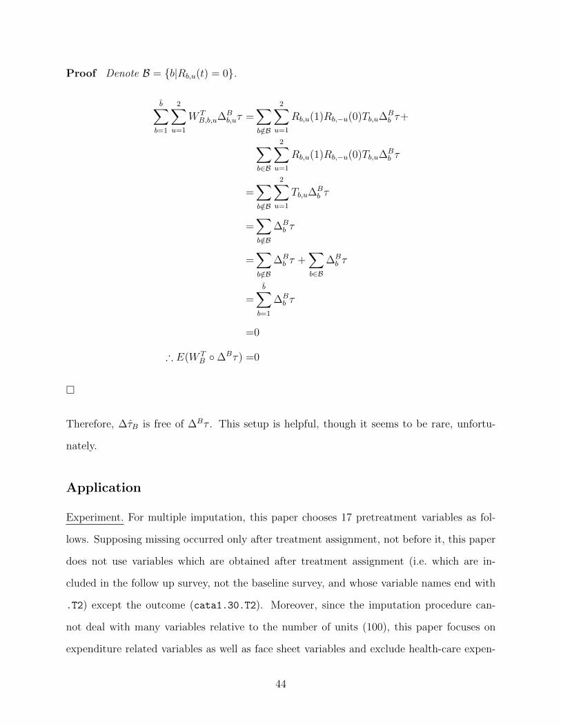
Proof Denote B = {b|Rb,u(t) = 0}.

b∑b=1

2∑u=1

W TB,b,u∆B

b,uτ =∑b/∈B

2∑u=1

Rb,u(1)Rb,−u(0)Tb,u∆Bb τ+

∑b∈B

2∑u=1

Rb,u(1)Rb,−u(0)Tb,u∆Bb τ

=∑b/∈B

2∑u=1

Tb,u∆Bb τ

=∑b/∈B

∆Bb τ

=∑b/∈B

∆Bb τ +

∑b∈B

∆Bb τ

=b∑

b=1

∆Bb τ

=0

∴ E(W TB ◦∆Bτ) =0

�

Therefore, ∆τB is free of ∆Bτ . This setup is helpful, though it seems to be rare, unfortu-

nately.

Application

Experiment. For multiple imputation, this paper chooses 17 pretreatment variables as fol-

lows. Supposing missing occurred only after treatment assignment, not before it, this paper

does not use variables which are obtained after treatment assignment (i.e. which are in-

cluded in the follow up survey, not the baseline survey, and whose variable names end with

.T2) except the outcome (cata1.30.T2). Moreover, since the imputation procedure can-

not deal with many variables relative to the number of units (100), this paper focuses on

expenditure related variables as well as face sheet variables and exclude health-care expen-

44

diture variables (except cata1.30 in the baseline survey, which corresponds to the outcome

(cata1.30.T2 in the follow up survey)) due to high correlation among them. Nominal

variables (cluster ID and its counterpart ID) and a constant variable (BMI) are also dis-

carded. Finally, four variables (sp.op, hhage (age of head of household), hheduc (education

of head of household), and interact) are dropped because they are highly correlated with

other variables. After this procedure, 17 variables remain. Their names are assets, age,

sex, educ, hhsex, hhsize, in.sp, treatment, urbrur, indigenous, Oportunidades, margw,

dependents, media, P06D01, P12D01, and cata1.30. They overlap the variables King et al.

(2007, 492, f.n. 9) used for matching pairs.

Observational Study. The dataset file, cps1re74.dta, was downloaded from http://economics.

mit.edu/faculty/angrist/data1/mhe/dehejia (access on December 23, 2013). Readers

might be interested in websites of Dehejia and Wahba (1999).24 The nine matched-on vari-

ables which this paper utilizes for matching and multiple imputation are age, its square,

years of schooling, four indicator variables for blacks, Hispanics, martial status, and high

school diploma, real earnings in 1974, and real earnings in 1975. Following demonstration in

Matching package, the next version of the paper will also use three square terms of years of

schooling, real earnings in 1974, and real earnings in 1975.25 It will also add two unemploy-

ment dummies in 1974 and 1975. Since randomization occurred between March 1975 and

July 1977 (Dehejia and Wahba, 1999, 1054), real earnings in 1974 and real earnings in 1975

are pretreatment variables and real earnings in 1978 is a post-treatment outcome.

24 http://users.nber.org/~rdehejia/nswdata.html and http://users.nber.org/~rdehejia/

nswdata2.html.25 http://sekhon.berkeley.edu/matching/DehejiaWahba.Rout. As for Matching package and its com-

panion papers, see http://sekhon.berkeley.edu/matching/.

45