Electronic copy available at: http://ssrn.com/abstract=1107690

MISPRICING FOLLOWING PUBLIC NEWS:

OVERREACTION FOR LOSERS, UNDERREACTION FOR WINNERS

Ferhat Akbas, Emre Kocatulum, and Sorin M. Sorescu*

March 17, 2008

ABSTRACT

We document an important relation between two well-established anomalies: momentum and short-term reversal. Only stocks with negative momentum experience short-term reversal. Using Chan’s (2003) news database, we show that the market appears to overreact to public news following bad past performance and underreact following strong past performance. The results are robust to using alternative methodologies. Stocks with current good news and negative momentum earn on average –9.3% annual raw returns during the subsequent month, while stocks with current good news and positive momentum earn +32.2%. The large, negative raw returns point to cognitive biases, rather than risk-based explanations, as the source of abnormal returns.

* Akbas and Sorescu are from Mays Business School at Texas A&M University. Kocatulum is from the Massachusetts Institute of Technology. The authors thank Wesley Chan for graciously sharing the news data, as well as Kerry Back, Ekkehart Boehmer, and Michael Gallmeyer for useful comments and suggestions. Please address correspondence to Sorin Sorescu at Texas A&M University, at ssorescu@tamu.edu, or +1 979 458 0380.

Electronic copy available at: http://ssrn.com/abstract=1107690

2

MISPRICING FOLLOWING PUBLIC NEWS:

OVERREACTION FOR LOSERS, UNDERREACTION FOR WINNERS

March 17, 2008

ABSTRACT

We document an important relation between two well-established anomalies: momentum and short-term reversal. Only stocks with negative momentum experience short-term reversal. Using Chan’s (2003) news database, we show that the market appears to overreact to public news following bad past performance and underreact following strong past performance. The results are robust to using alternative methodologies. Stocks with current good news and negative momentum earn on average –9.3% annual raw returns during the subsequent month, while stocks with current good news and positive momentum earn +32.2%. The large, negative raw returns point to cognitive biases, rather than risk-based explanations, as the source of abnormal returns.

3

The weak-form Efficient Market Hypothesis holds that stock returns cannot be predicted

based on past price behavior (Fama, 1970). Therefore, any study that attempts to present

the existence of abnormal returns based on information obtained from past prices is at

odds with even the weakest form of the Efficient Market Hypothesis. However, during

the past three decades, the literature documented three types of return predictability

anomalies, all based on historical price patterns. In the cross-section, stock returns

present with reversal (or overreaction) at long-term intervals of three to five years,

momentum (or underreaction) at medium-term intervals of six to twelve months, and

again reversal (or overreaction) at short-term intervals of one or four weeks.1

In response to Fama’s (1998) call for a unified theory of behavioral finance that can

simultaneously explain over- and underreaction, the literature responded with several

behavioral models that link long-term reversal and medium-term momentum patterns.

For example, Daniel, Hirshleifer and Subrahmanyam (1998) propose a model which

incorporates investor’s overconfidence about private signals leading to medium-term

underreaction to public news and long-term overreaction to private signals. Barberis ,

Shleifer and Vishny (1998) presents a model in which investors are misinformed about

the statistical properties of earnings and therefore believe in either contrarian or trend-

following forecasting, which results in medium-term continuation and long-term reversal.

And Hong and Stein (1999) derive similar implications through a model with news-

watchers and trend followers.

1 See, e.g. DeBondt and Thaler (1985) who document reversal at three- to five-year intervals; Jegadeesh

and Titman (1993) who document momentum at three- to twelve-month intervals. Short term reversal is documented by Lehmann (1990) for weekly returns and by Jegadeesh (1990) for monthly returns.

4

By contrast, little is known about the relation between (medium-term) momentum and

short-term reversal.

We examine the interaction of momentum and short-term reversal and show that reversal

occurs only in stocks with negative momentum. Using Chan’s (2003) public news data

we explain reversal as a short-term overreaction to public news for stocks with negative

momentum. At the same time, we document a short-term underreaction to public news

for stocks with positive momentum.

To our knowledge, the magnitude of the abnormal returns resulting from this anomaly is

one of the largest ever documented in the literature. A hedge portfolio that is long in

stocks with good news and positive momentum, and short in stocks with good news and

negative momentum, earns a remarkable 46.3% per year after controlling for the Fama-

French factors, even after excluding stocks priced at less than $5 a share.

A possible explanation for this anomaly is that it represents a priced, unknown risk factor.

Risk-based explanations suggest that any abnormal returns are fair compensation for risk,

and do not necessarily contradict the Efficient Market Hypothesis. For example, Chan

(1988), Ball and Kothari (1989), and Zarowin (1990) all propose risk-based explanations

for the DeBont and Thaler (1985) long-term reversal anomaly.

5

We believe that risk-based explanations are not consistent with the results presented in

our study, simply because stocks with negative momentum and good news earn negative

raw returns of approximately -9.3% per year, during more than two decades. To justify a

negative risk premium of this magnitude, these stocks’ dividend payoffs would have to be

highest in those states of the world for which the aggregate output is low (and which

carry high Arrow-Debreu state prices). Yet, these stocks are shown to load positively on

all three Fama-French risk factors, suggesting that their expected rate of return should be

positive.

In the absence of a reasonable risk-based explanation, we believe that the anomaly is

driven primarily by cognitive biases. In the discussion section we propose an explanation

which draws from the psychology literature in the areas of cognitive dissonance and

overconfidence. In doing so, our goal is not to identify the precise cognitive bias that is

at the origin of this new anomaly, but rather to suggest a plausible explanation and to

initiate an academic dialogue that would enhance our understanding of price formation

under non-Bayesian updating.

The next section presents data sources and descriptive statistics. Section II shows that

short-term reversal occurs only in stocks with negative momentum. Section III explores

the role of public news, and Section IV presents an explanation based on the literature in

psychology. Section V concludes.

6

I. DATA SOURCES AND DESCRIPTIVE STATISTICS

Our main dataset include all stocks traded on NYSE, AMEX and NASDAQ during the

period from 1980 to 2006. Stock returns are obtained from the Center for Research in

Security Prices (CRSP) at University of Chicago. All returns are corrected for de-listing

to avoid survivorship bias. Following Jegadeesh and Titman (2001), we exclude stocks

with a share price below $5 at the portfolio formation date to make sure that the results

are not driven by small, illiquid stocks or by bid–ask bounces.

Momentum is measured as the cumulative raw return from month t-6 to t-1. To measure

reversal we compare stock returns between months t and t+1. We define “reversal” as a

situation where returns at month t+1 are of the opposite sign of those at month t. If the

two returns are of the same sign, we refer to it as “continuation.”

To examine stock price responses to public news, we employ a news dataset assembled

by Chan (2003), which covers a random sample of approximately one-quarter of all

CRSP stocks over the period from 1980 to 2000.2 Chan (2003) maintains a count of

news items obtained from Dow Jones Interactive Publications Library of past

newspapers, looking at only publications with over 500,000 current subscribers. For each

2 We are grateful to Wesley S. Chan for sharing his dataset.

7

stock covered, the dataset collects the dates at which the stock was mentioned in the

headline or lead paragraph of an article of one of the publications covered.3

II. RELATION BETWEEN MOMENTUM AND SHORT-TERM REVERSAL

A. Univariate Analysis

We begin with a univariate analysis of the momentum and reversal effects. At this point

our goal is only to replicate the findings of Jegadeesh (1990), and of Jegadeesh and

Titman (1993) with our new sample. Table II presents the results.

Panel A of Table II presents the momentum effect. Stocks are sorted into deciles based

on their cumulative returns during months [t-6, t-1], and the returns of each decile are

measured at month t+1. Consistent with Jegadeesh and Titman (1993), we observe a

near-monotonic positive relation between past and future returns. Moreover, this relation

is significant at high levels (t=6.14) as evidenced by the return of the hedge portfolio that

is long past winners and short past losers.

Panel B of Table II presents the reversal effect. Stocks are sorted into deciles based on

their returns during month t, and the returns of each decile are measured at month t+1.

Here, the best performers in any month are the losers from the previous month, and vice-

versa. And the returns on the hedge portfolio show that this effect is statistically

3 For a more detailed description of the dataset see Chan (2003)

8

significant (t=-2.59). We thus confirm Jegadeesh’s (1990) finding of stock price reversal

for the one-month horizon.

B. Interaction between Momentum and Reversal.

We now seek to understand the relation between momentum and reversal. We do so by

relating returns at month t+1 to the interaction of returns measured during [t-6, t-1]

(momentum), and those measured during month t (reversal). As is common with this

type of studies (Jegadeesh and Titman, 1993; Avramov et al., 2006; Jegadeesh, 1990;

Chan, 2003), we use two econometric approaches: calendar-time portfolios and Fama-

MacBeth regressions.

B.1. Calendar Time Portfolios

We assign stocks to quintiles based on momentum measured during [t-6, t-1]. We also

independently sort each quintile into five portfolios based on stock returns measured

during month t. The returns of the resulting 25 portfolios are measured during month

t+1. The monthly mean returns are then averaged intertemporally and the results are

presented in Table III. The last two lines of Table III show the performance of a hedge

portfolio that is long past month’s losers and short past month’s winners. A separate

hedge portfolio is constructed for each momentum quintile.

A reversal effect occurs when there is a monotonically decreasing relation between

returns at month t (denoted R1, R2 … R5) and returns at month t+1. The statistical

9

significance of any reversal relation is measured with the hedge portfolio at the bottom of

the table.

Surprisingly, we find that reversal only occurs for stocks with negative momentum (M1

and M2). Moreover, this reversal is strongest in the lowest (M1) momentum category.

In that case, the hedge portfolio earns a mean monthly return of 1.76%, with a high level

of statistical significance (t=7.89). By contrast, there is no evidence of reversal among

high-momentum stocks (M5). In that case, the hedge portfolio earns an insignificant

0.48% return per month, during the same period.

B.2. Fama-MacBeth Regressions

We repeat the analysis from Table III using Fama-MacBeth regressions. Each month t,

we sort stocks into five quintiles based on their momentum measured during [t-6, t-1].

We then run cross-sectional regressions of the return at month t+1 on the return at month

t, for each of the five momentum portfolios. As in Fama and MacBeth (1973), we

compute the final coefficients from the inter-temporal average of month-specific

regression estimates.

The results are presented in Table IV. We observe a striking difference between the

monthly serial correlation within the low (M1) and high momentum (M5) portfolios. As

before, reversal occurs only in the lowest two momentum portfolios. For M1, reversal is

highest with a coefficient of -0.0491 (t=-9.93). These results are consistent with those

reported in Table III.

10

C. Robustness Tests

We now reexamine our results with the goal of assessing their robustness. We repeat our

tests with plausible changes in asset pricing models and econometric approaches.

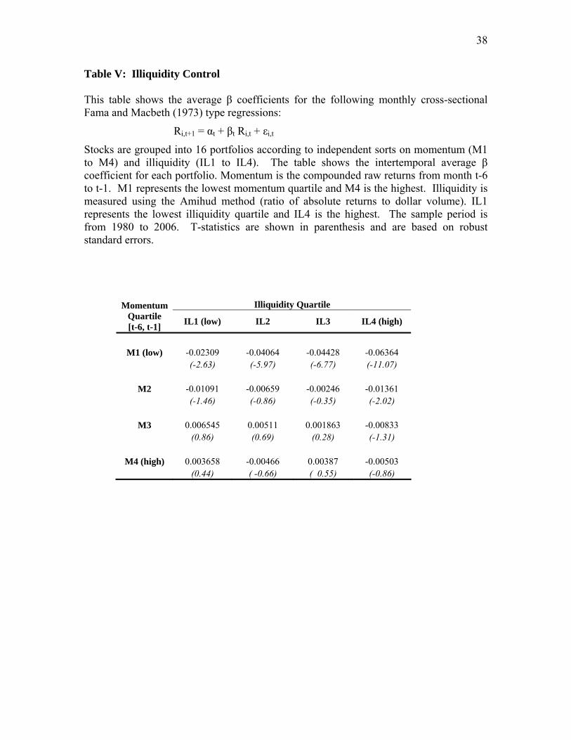
C.1. Illiquidity

Avramov et al. (2006), suggest that short-run contrarian profits are driven by illiquidity,

consistent to the rational equilibrium framework of Campbell et al. (1993). They show

that weekly reversal is stronger for stocks with high illiquidity, and implicitly argue that

illiquidity is also a driver of monthly return reversals. If the low momentum stocks are

also the most illiquid, our results could be driven by liquidity effect. We now introduce a

liquidity control in our analysis.

Our proxy for illiquidity is the Amihud (2002) measure, which is computed as the

absolute price change per dollar of daily trading volume. To control for illiquidity, we

first sort stocks into four momentum quartiles, and also independently sort stocks into

four illiquidity quartiles. In each of the resulting 16 portfolios, we perform cross-

sectional Fama-Macbeth (1973) regressions, and compute the intertemporal mean of the

beta coefficients:

Rit+1 = αt + βt Rit + εit (1)

11

If our results are driven by illiquidity rather than momentum, then we should not observe

any significant difference among β coefficients within the same illiquidity quartiles.

Moreover, the β coefficients should be significantly negative only among the high

illiquidity stocks. By contrast, if the momentum effect persists independent of illiquidity,

we should observe significantly negative beta coefficients for all low momentum stocks.

Table V presents the results. Each cell in Table V shows the intertemporal average of

Fama-MacBeth beta coefficients obtained from Equation (1). The data show a clear

illiquidity effect, in that reversal is stronger (betas are more negative) for stocks with

higher illiquidity.

However, our results are not driven by illiquidity. The momentum effect is always

significant regardless of the illiquidity level. Among low illiquidity stocks (IL1), the

average β from equation (1) increases monotonically with momentum, from -0.02509

(t= -3.18) to 0.00387 (t=0.46). A similar increase is noticed among high illiquidity stocks

(IL5): the average β from equation (1) increases monotonically from -0.056 (t=-9.5) to

-0.00427 (t=-0.68).4 Moreover, among stocks with low momentum (M1), the reversal

effect is always statistically significant, regardless of the level of liquidity. We conclude

that while illiquidity moderates the relation between momentum and reversal, it does not

explain it.

4 In all illiquidity quartiles, the momentum effect is found to be statistically significant at the 1% level (not

shown).

12

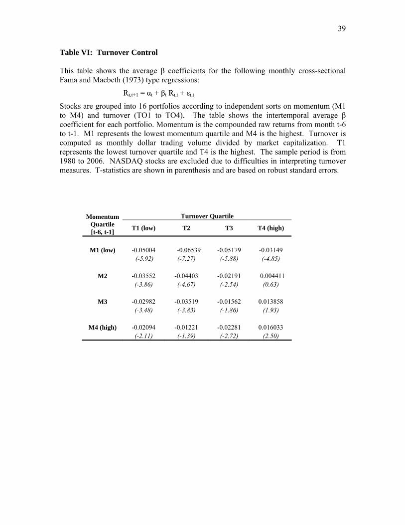
C.2. Turnover

Campbell, Grossman, and Wang (1993) propose a rational expectations explanation for

the reversal effect. They argue that non-informed trading causes price movements that,

when absorbed by liquidity suppliers, cause prices to revert. This suggests that non-

informed trading is accompanied by high trading volume, while low volume reflects

informed trading. If our results are entirely explained by the rational expectations model

of Campbell et al., the reversion effect should be affected only by trading volume, not

momentum. Conrad, Hameed, and Niden (1994) find support for the Campbell et al.

model, at weekly frequencies.

We control for trading volume using monthly turnover measures computed as the

monthly dollar trading volume divided by market capitalization. We use the same

method as in the previous sub-section where we controlled for illiquidity. However, as

suggested in Lee and Swaminathan (2000), we exclude all NASDAQ stocks to avoid

problems with inflated trading volume caused by double counting dealer trades.

The results are presented in Table VI. The interaction of momentum and reversal

remains persistent even after controlling for turnover. The effect of momentum is always

significant regardless of the illiquidity level. Among low turnover stocks (T1), the

average β from equation (1) increases with momentum from -0.05007 (t=-6.20) to

-0.03234 (t=-5.19). Similarly, among high turnover stocks (T5) the average β increases

with momentum from -0.01918 (t=-1.85) to 0.01713 (t=2.76). The differences are always

significant at 1% level. Most importantly, for low momentum stocks, the reversal effect

13

is always significant regardless of turnover. As with the case of illiquidity, we conclude

that while turnover is an important moderator of the relation between momentum and

reversal, it does not explain it.

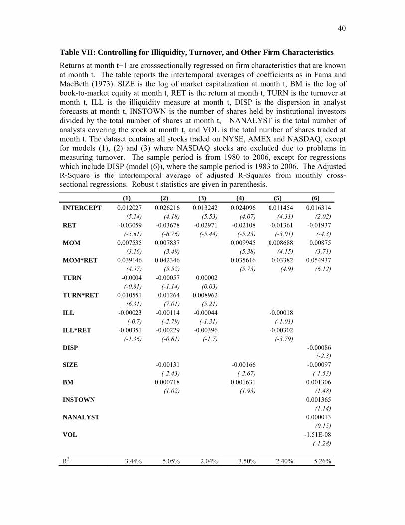
C.3. Multiple Controls

Until now we have shown that the momentum-reversal relation survives controlling for

illiquidity and, independently, turnover. But will the relation remain significant if we

control for both effects simultaneously? To answer this question we conduct Fama-

Macbeth regressions on the entire sample. We also include other firm characteristics that

are known to be associated with the cross-section of stock returns: book-to-market,

dispersion of analyst forecast, institutional ownership, and number of analysts covering

the firm.

The results are presented in Table VII. Our focus is on the interaction coefficient of

momentum and current monthly returns (MOM*RET). The interaction coefficients are

always positive and highly significant, suggesting that the reversal effect diminishes as

momentum increases, regardless of which control variables are used in the statistical

specification. This is again consistent with our previous findings.

C.4. Dependent Sorts

All calendar time portfolio results that depend on two variables are derived from

independent sorts on the two variables. For example, in Table III, stocks are sorted

independently on momentum and current returns. We re-do all tests with dependent

14

sorts, sorting first by momentum then by the other variable within each momentum

group. The results (not shown) are almost identical in terms of magnitudes and statistical

inferences.

C.5. Small Cap Screen

We repeat our tests after excluding all small cap stocks from the analysis. Industry

professionals place the boundary between small- and mid-cap stocks anywhere from one

to two billion dollars. In the absence of a clear consensus, we use a threshold of $1.5

billion for stocks traded in December 2006. For months prior to December 2006, we

deflate the $1.5 billion value with the CRSP value-weighted return index (including

dividends). We then eliminate all stocks whose market value falls below the $1.5 billion

threshold (or the deflated value thereof). The results (not shown) are almost identical in

all respects.

C.6. Different Momentum Definitions

Jegadeesh and Titman (1993) show that the momentum effect is robust to measurement

periods ranging from three to months. As a result, we repeat our analysis with

momentum redefined as cumulative returns measured alternatively over months [t-3, t-1],

[t-9, t-1], and [t-12, t-1]. Our results (not shown) are not affected by these alternative

measurement horizons.

15

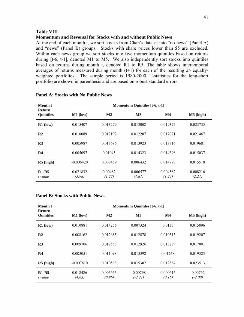
III. THE ROLE OF PUBLIC NEWS

In the previous section we document that reversal occurs exclusively among low

momentum stocks. We now show that this result is driven by the differential response of

low- and high-momentum stocks to public news.

We obtain a count of public news from Chan’s (2003) dataset. His is the first paper to

document the importance of public news for monthly mean reversals.5 Every month,

Chan (2003) separates his data into two groups: stocks that were mentioned in the

headline or lead paragraph of an article from a publication with more than 500,000

current subscribers (news stocks) and other stocks (no news stocks). He then looks at

monthly serial correlation patterns for these two different groups. He finds reversal only

for the “no news” sub-sample. By contrast, monthly serial correlation is not significant

for the “news” sample. Chan’s analysis, however, does not explore the role of

momentum, mainly because his paper focuses primarily on explaining long term

anomalies as opposed to the interaction between momentum and short-term (monthly)

reversal.

A. “News” and “No News” Samples

We examine the effect of momentum on the reversal effect separately for the “news” and

“no news” sub-samples. Our focus is on the “news” sub-sample where Chan found no

significant monthly serial correlation of any sign. We will show that Chan’s zero-serial-

5 Pritamani and Singal (2001) collected daily news stories from the Wall Street Journal and Dow Jones

News Wire for a subset of less than 1% of CRSP stocks, during only the period from 1990 to 1992.

16

correlation result is in fact the average of two distinct economic realities: reversal for

low-momentum stocks, and continuation for high-momentum stocks. Our analysis uses

the same news dataset collected by Chan (2003), which spans a time period from 1980 to

2000. Following Jegadeesh and Titman (2001), we again exclude stocks with a share

price below $5 at the portfolio formation date, to ensure that the results are not driven by

small, illiquid stocks or by bid–ask bounces.

Following Chan, we divide stocks into two groups: Stocks that were mentioned in the

headlines (the news group) based on Chan’s dataset, and stocks that were not (the no-

news group). We repeat our previous analysis with these two sub-samples. For

conciseness, we present only the results obtained with portfolio sorts; the results based on

the Fama-MacBeth method are very similar. Within each sub-sample (news and no-

news), every month we sort stocks into five groups according to momentum month t-6 to

t-1. We then independently sort stocks into five groups according to the rate of return

observed that particular month, t.

The results are presented in Table VIII. Panel A of Table VIII replicates Chan’s finding.

We show that stocks with no public news present with reversal for all momentum

portfolios. By contrast, the results form the “news” sub-sample, shown in Panel B are

new and intriguing. Recall that Chan had found zero serial correlation for this sub-

sample without conditioning on momentum. Once we condition on momentum, we find

strong negative serial correlation (reversal) among stocks with low momentum, and

strong positive serial correlation (continuation) among stocks with high momentum.

17

B. Economic Significance

The results from Table VIII, especially those in Panel B suggest that there is significant

mispricing among stocks with public news, high current return, and extreme (high or

low) momentum. Stocks with high current returns and high momentum [M5, R5] earn an

average monthly raw return of 2.35% during the subsequent month. At the other extreme

the average monthly raw return for stocks with low momentum and high current returns

[M1, R5] is -0.76%. The differential performance between these two groups (3.29% per

month) suggests a mispricing of a remarkable magnitude. To our knowledge, no other

study finds hedge portfolio returns even close to 3% per month, especially after

eliminating small stocks.

To understand the full economic significance of this mispricing, we compute annual

returns for the long, short, and hedge portfolios for each year during the sample period.

We also inquire if the mispricing is due to the well-known January effect. The results are

presented in Table IX. The large, top section of the table shows annual percentage

returns for the three portfolios and for two popular benchmarks: the SP500 and the CRSP

value-weighted return including dividends. The third line from the bottom shows the

average annual return computed during the months of January only. The second line

from the bottom shows average annual returns computed each year from the months of

February to December. The last row in Table IX shows the average annual returns for all

stocks, for the entire sample period.

18

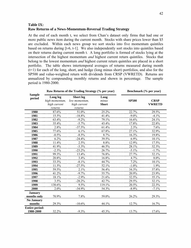
We observe that the hedge (long minus short) portfolio produces positive raw returns in

every single year in our sample. Moreover, this portfolio beats the SP500 in all but three

years. Other performance statistics are also favorable. For example, the volatility of the

hedge portfolio is 21.3% per year and its Sharpe ratio is a remarkable 2.1 (not shown in

the table). This compares favorably to a volatility of 15.1% and a Sharpe ratio of 0.92 for

the SP500 portfolio.

Although a mild January effect is present, it cannot be the source of this anomaly. The

hedge portfolio earns 59.0% per year during January and 44.1% per year during the

months of February to December. The average annual performance of the hedge

portfolio is 45.3% over the twenty-one-year sample period. To our knowledge, this is the

largest magnitude for equity long-short strategies that has been documented in the

literature.

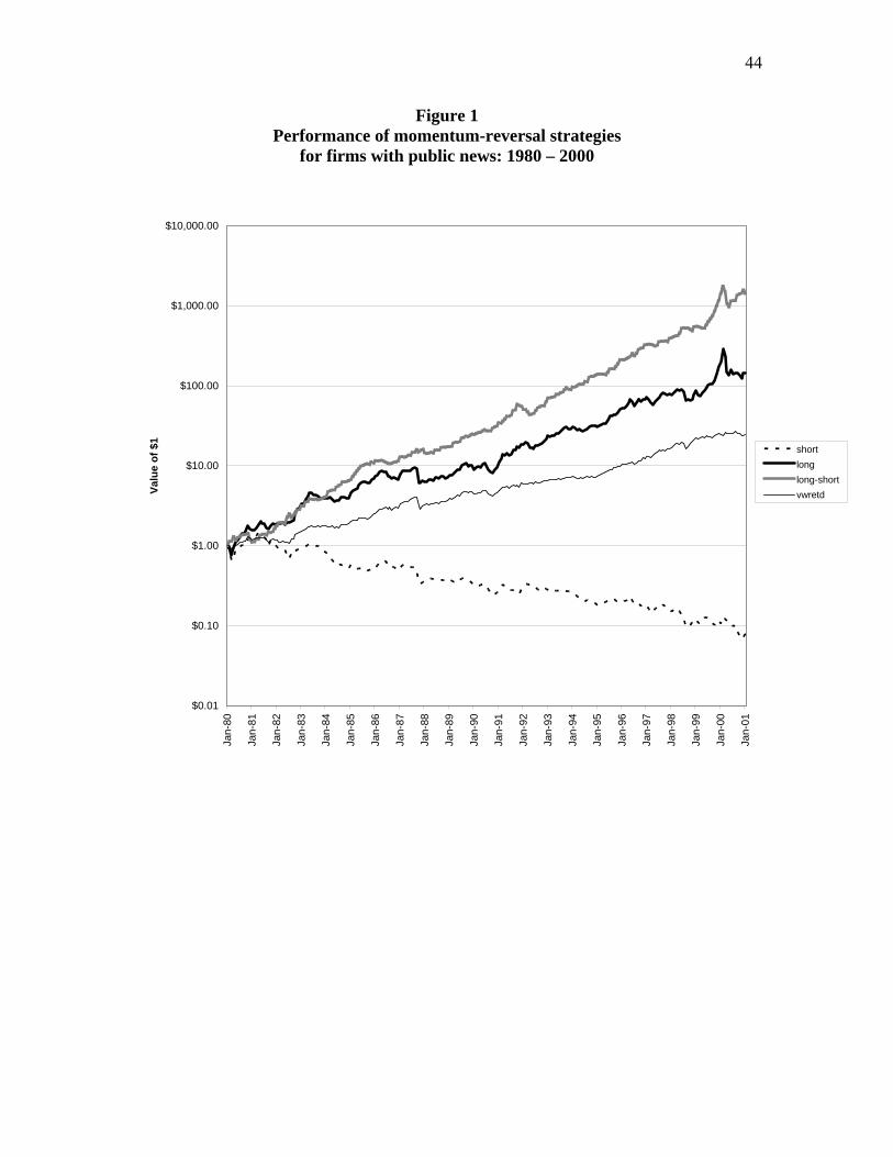
Figure 1 provides a visual depiction of the economic importance of our findings. All four

lines show the cumulative value of a one-dollar investment made during the month of

January 1980. The top line in the figure depicts the performance of the hedge portfolio

based on the news-momentum-reversal strategy. The second line from the top shows the

performance of only the long leg of that hedge portfolio. The bottom line shows the short

leg of the hedge portfolio, except that the performance is shown from the buyer’s

19

perspective and not that of the short-seller.6 The remaining (thin) line shows the

performance of the value-weighted market index.

It is immediately apparent that the performance of the hedge portfolio is clearly superior

to that of the benchmark. One dollar invested in January 1980 grows to $1,425 with the

actively managed strategy, compared to only $24 in the market index. Also remarkable is

that our strategy can identify a set of stocks with negative raw returns of a significant

magnitude. If an inadvertent investor would take a long position in stocks belonging to

the short portfolio, that investor would lose more than 90% of its initial investment. The

dollar invested in 1980 would be worth less than 8 cents at the end of 2000. To our

knowledge, we are the first to identify an anomaly that produces negative raw returns of

this magnitude. Most other anomalies document negative abnormal returns.

This particular finding has a very important implication in light of the popularity of risk-

based explanations of financial anomalies. When an anomaly produces negative

abnormal but positive raw returns, it could be consistent with either mispricing or lower

risk premium. A good example is Johnson (2004) who observes that stocks with high

dispersion of opinion have negative abnormal returns (which are nonetheless positive on

a raw basis). He proposes an option-theoretic, rational expectations model to explain this

result. However, when an anomaly produces negative raw returns equal to -9.3% per

year for over 20 years, there is little that risk-based explanations can do to make it

consistent with rational expectations. Indeed, any such explanation is held to the high

6 Thus, the negative performance depicted in the graph implies positive profits for the short-seller.

20

standard of providing direct evidence that such stocks could have a negative expected

rate of return in equilibrium.7 In short, we believe that the results of our short portfolio

present what is perhaps the most unambiguous evidence of mispricing ever documented

in the literature.

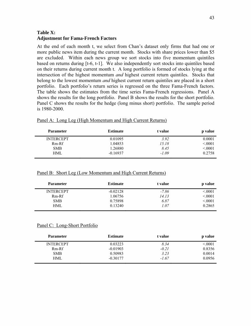
In Table X we re-examine the performance of the long, short, and long-short portfolios

after controlling for the Fama-French factors. Not surprisingly, the long portfolio (Panel

A) presents with a significantly positive abnormal return. In Panel B, we observe a

negative abnormal return for the short portfolio. More interesting however are the

loadings on the Fama-French factors for the short portfolio. These loadings are all

positive, suggesting that the risk premium should also be positive, at least as captured by

the Fama-French factors. The positive risk loadings from Panel B present prima-facie

evidence that the negative raw returns from Table IX represent true mispricing as

opposed to a (negative) risk premium.

The results of the long-short portfolio (Panel C) show a remarkable 3.22% monthly

abnormal return for a strategy that is essentially market-neutral (β=-0.02, t=-0.21). Since

the theoretical return of any market neutral strategy is the risk-free rate, the size of the

long-short abnormal returns is clearly indicative of significant mispricing.

7 We recognize that negative expected returns are possible in equilibrium, but only in the case of assets

whose cashflows are negatively correlated with the aggregate output. Thus, a risk-based explanation can only be convincing if it presents clear evidence of such negative correlation.

21

IV. DISCUSSION

We have documented significant mispricing for stocks with good news and extreme

momentum. The magnitude of the mispricing, as well as the large, negative raw returns

obtained for stocks with low momentum and good current news, point to behavioral,

rather than risk-based explanations for this anomaly.

Specifically, we observe that stock prices overreact – at the one-month horizon – to

public news when the momentum is negative. For this group of stocks we see a strong

reversal in returns between month t (when the news arrives) and month t+1 (when,

presumably, prices begin to return towards equilibrium).

By contrast, for stocks with positive momentum prices underreact to public news at the

one-month horizon. In this case, returns from month t continue unto month t+1 in the

same direction.

The price response pattern we document here is new to the finance literature. We are the

first to document an anomaly where separate stock groups simultaneously overreact and

underreact to news, depending upon each group’s price history. Moreover, this

differential reaction occurs for the same, short term, horizon. We refer to this type of

anomaly as cross-sectional differential reaction. It contrasts with time-series differential

reaction documented in prior literature, where the same group of stocks presents with

22

both over- and under- reaction at different time horizons (such as 3-12 months

momentum and 3-5 years reversal).

The cross-sectional differential reaction anomaly cannot be readily explained by the

prominent theoretical models from the behavioral finance literature, mainly because such

models focus primarily on explaining the existing evidence of time-series differential

reactions (e.g. Daniel, Hirshleifer, and Subrahmanyam, 1998). As a result, we turn to the

literature in cognitive psychology in search of an explanation. We look for factors that

link information processing (reaction to news) to past history (momentum).

We draw from the work done in the areas of cognitive dissonance and overconfidence,

and believe that our results are consistent with their key predictions. We present below a

conceptual behavioral framework that could produce the type of anomaly reported in this

paper. We hasten to add, however, that we view this framework as exploratory in nature.

Our main objective is to show that psychology theory could explain differential reaction

not only in time series but also in the cross-section. That is, depending upon investors’

ex-ante cognition, stock prices could either underreact or overreact to public news for the

same (short-term) time horizon. This is an important contribution in view of Fama’s

(1998) critique that behavioral theories fail to produce a unified theoretical body of

knowledge that can explain a large class of anomalies. Of course, we also hope that our

discussion here will stimulate additional research related to the effect of cognitive

dissonance and overconfidence on the price formation mechanism.

23

We should also add that we are at this point concerned only with the differential price

reaction among stocks with public news. Recall that this reaction is documented in Panel

B of Table VIII, as well as in Tables IX, X and Figure 1. This is because for this group

of stocks we can confidently attribute (at least part of) month t return to information

conveyed by public news that month.8 We do not attempt to explain the apparently

homogeneous under-reaction of stocks with no public news (Panel A of Table VIII),

because we are not sure to what causes we should attribute the returns observed at month

t for this other group of stocks.

A. Cognitive Dissonance

Pioneered by Festinger (1957), the concept of cognitive dissonance is the mental conflict

people experience when presented with evidence that is inconsistent with their prior

beliefs (Shiller, 1999). Festinger argues that faced with cognitive dissonance people will

take actions to minimize it, even if such actions appear irrational. Indeed, eliminating

dissonance appears to be one of humans’ most basic psychological needs.

In a classic experiment, subjects were asked to work on some tasks that were inherently

boring. Some of the subjects were manipulated by the experimenter into believing that

the tasks were in fact exciting. This created a state of cognitive dissonance for this group

of subjects. Seeking to reduce dissonance, those same subjects eventually changed their

beliefs and agreed that the tasks were exciting. The results suggest that people are

8 This follows Chan (2003).

24

uncomfortable to be in a dissonant state, and that one way to reduce dissonance is to

abandon one’s prior set of beliefs in favor of an alternative set that is more consistent

with public evidence (i.e. seeing a boring task as interesting, because the experimenter

claims it is interesting). Most importantly, this paradigm change occurs even in the

absence of any rational basis to embrace the alternative set of beliefs (the experimenter’s

opinion about the task does not change the fact that an intrinsically boring task remains

boring).

B. Overconfidence.

Langer and Roth (1975) are the first to document overconfidence as a cognitive bias. In

their experiment, subjects who are manipulated into believing to have superior skill sets

are confident that they can not only predict coin tosses but also affect their outcome.

Their finding has been repeatedly replicated, and it is now generally accepted among

psychologists that people show excessive confidence about their own judgments.

Overconfidence has also been extensively studied in the behavioral finance literature.9

As Shiller (1999) observes, overconfidence does not in itself predict whether prices will

respond to news with an over- or underreaction pattern. Rather, it simply predicts that

overconfident people will make errors, but not in any well-specified direction. By

contrast, we believe that when overconfidence is analyzed together with cognitive

dissonance, it has the potential to explicate cross-sectional differential reactions such as

the ones documented in our study.

9 See, Shiller (1999) for a review of the behavioral finance literature on overconfidence.

25

C. Relation to Empirical Results.

To relate our findings with cognitive dissonance we begin with the observation that

investors are net long in the stock market, and by a wide margin.10 We also assume that

investors are overconfident in their own judgment. Moreover, we assume that this

overconfidence plays a key role at the time of stock purchase: investors select only those

stocks for which they have favorable private beliefs that indicate expected positive

returns. In short, we assume that investors only purchase stocks on which they expect to

make money, and feel quite confident with their choices.

We then take the view that in the cross-section of stock returns, among stocks with low

momentum (i.e. negative past returns), the investor base is more likely to include people

in a state of severe cognitive dissonance – those who purchased the stock moths ago with

the expectation that it would increase in value, but nevertheless faced the obvious reality

of a severe price depreciation.

By contrast, the investor base for high-momentum stocks (those with positive past

returns) will not likely face any cognitive dissonance. These investors probably feel good

about their choices and attribute the stock’s performance to their own stock picking

10 This is substantiated by the fact that the average ratio of short interest to total shares outstanding is quite

low. For example, this ratio was approximately 0.7% in the 1980s and 1.2% in the 1990s.

26

abilities.11 When faced with this type of cognitive consonance, investors remain

overconfident about their own private signals of firm quality and are thus likely to

overweigh them when compared to public signals.12 Public news will therefore be

underweighed as investors adjust their expectations in a non-Bayesian manner and

continue place excessive weight on their own private signal, as they did at the time of the

initial stock purchase. This results in underreaction to public news (both good and bad)

for high-momentum stocks, consistent with the evidence presented in this paper.

Returning now to negative-momentum stocks, if the investor base is significantly affected

by cognitive dissonance, a paradigm shift will occur with the arrival of public news.

Similar to the shift documented by Festinger (1957) in his classic experiment, these

investors will now abandon their previous paradigm of relying primarily on private

signals and instead adopt the alternative paradigm that public signals are more

informative about firm quality. Due to overconfidence, they will place a higher-than-

normal weight on the public signal. This causes stock prices to overreact to public news

(both good and bad) for stocks with negative momentum.

At this point, an important observation is warranted. One could also interpret our

empirical results to imply that investors are overconfident in the case of low momentum

stocks (where prices overreact), and underconfident for high momentum stocks (where

11 This relates to the “self attribution bias” proposed by Daniel, Hirshleifer and Subrahmanyam (1998), and

also to the psychological concept of “illusion of control” and “magical thinking.” Shiller (1999) provides an excellent review of studies in these two latter areas.

12 The concept of cognitive consonance is the opposite of cognitive dissonance and refers to situations when people are presented with evidence that conforms to their prior beliefs.

27

prices underreact). Indeed, the concepts of overreaction and underreaction are often

taken as synonymous to overconfidence and underconfidence (respectively), but this need

not be the case (Shiller, 1999). This alternative explanation is less than satisfactory

because it does not meet Fama’s (1997) test of forming a unified theory. Why would

investors, in the cross-section, be underconfident in some cases and overconfident in

other?

By contrast, our proposed explanation has the unique advantage of treating

overconfidence and cognitive dissonance as universal phenomena that are present among

all groups of investors. In the cross-section of stock returns, overconfidence can manifest

in either overreaction or underreaction depending upon investor’s cognition (dissonant or

consonant), which is itself predictable.

V. SUMMARY AND CONCLUSION

We examine the interaction of momentum and short-term reversal. Although each of

these two effects is well documented in the finance literature, the relation between the

two is not well understood. We show that reversal occurs only for stocks with negative

momentum. Moreover, using Chan’s (2003) news database we find that the reversal

effect suggests overreaction to public news for stocks with negative momentum. By

contrast, for stocks with large, positive momentum, we find underreaction to public news.

28

These findings present opportunities for earning abnormal returns of a magnitude never

before documented in the literature. A market-neutral hedge portfolio long on stocks

with good news and positive momentum and short on stocks with good news and

negative momentum earns well over 40% per year, even after accounting for the Fama-

French factors. Even more remarkable is that the raw returns of stocks in the short leg of

the hedge portfolio are actually negative and large in magnitude (-9.3% per year). These

stocks load positively on the Fama-French factors, suggesting that their negative returns

are unlikely caused by negative risk premia or another type of rational explanation.

Our paper is also the first to document a case where overreaction and underreaction do

coexist in the cross-section of stock returns. This contrasts to prior behavioral finance

literature where these two phenomena are often viewed as affecting stock returns in the

time series, at different time intervals.

We propose a behavioral explanation to explain the link between momentum and the

differential reaction to public news. Our explanation draws from the behavioral concepts

of cognitive dissonance and overconfidence. Overconfident investors who hold stocks

with negative momentum are more likely to face cognitive dissonance when compared to

those who hold positive-momentum stocks. As a result, the former place excessive

weight on public news, leading to overreaction, while the latter place excessive weigh on

their private signals, leading to underreaction.

29

We hope that our study provides the impetus for more researchers to rely on theory from

cognitive psychology in explaining anomalous findings in the asset pricing literature.

Investors and analysts are, above all, humans, and as such are subject to the same biases

that have been thoroughly studied in the psychology literature. Five decades of research

in cognitive psychology provide rich insights to help us build a unified framework that

explains the menu of anomalies documented in the empirical asset pricing literature.

30

REFERENCES

Amihud, Yakov, 2002. Illiquidity and stock returns: Cross-section and time-series effects,

Journal of Financial Markets 5, 31–56.

Ang, Andrew, Robert J. Hodrick, Yuhang Xing and Xiaoyan Zhang, 2006a. The cross

section of volatility and expected returns, Journal of Finance 61, 259-299.

Avramov, D., T. Chordia, and A. Goyal, 2004. Liquidity and autocorrelations in

individual stock returns. Journal of Finance 61 (5), 2365–2394.

Ball, R., Kothari, S.P., 1989. Nonstationary expected returns: Implications for tests of

market efficiency and serial correlation in returns. Journal of Financial Economics

25, 51-74.

Ball, R., Kothari, S.P., Wasley, C.E., 1995. Can we implement research on stock trading

rules? Journal of Portfolio Management 21, 54-63.

Barberis, N., Shleifer, A., Vishny, R., 1998. A model of investor sentiment. Journal of

Financial Economics 49, 307-343.

Branch, B., 1977. A tax loss trading rule, Journal of Business 50, 198-207.

Campbell, J.Y., Grossman, S.J., Wang, J., 1993. Trading volume and serial correlation in

stock returns. Quarterly Journal of Economics 108, 905-939.

Chan, K. C., 1988. On the contrarian investment strategy. Journal of Business 61, 147-

163.

Chan, L.K., Jegadeesh, N., Lakonishok, J., 1996. Momentum strategies. Journal of

Finance 51, 1681-1714.

Chan, S.W., 2003. Stock price reaction to news and no-news: drift and reversal after

headlines. Journal of Financial Economics 70, 223-260.

31

Chopra, N., Lakonishok, J. and Ritter, J., 1992. Do stocks overreact? Journal of Financial

Economics 31, 235-268.

Conrad, J.S., Gultekin, M., Kaul, G., 1997. Profitability of short-term contrarian

strategies: Implications for market efficiency. Journal of Business and Economic

Statistics 15, 379-386.

Cooper, Michael, 1999. Filter rules based on price and volume in individual security

overreaction, Review of Financial Studies 12, 901–935.

Daniel, K.D., Hirshleifer, D., Subrahmanyam, A., 1998. Investor psychology and security

market under- and over-reactions. Journal of Finance 53, 1839-1885.

DeBondt, W.F.M., Thaler, R.H., 1985. Does the stock market overreact? Journal of

Finance 40, 793-808.

Diether, Karl B., Christopher J. Malloy, and Anna Scherbina, 2002. Differences of

opinion and the cross-section of stock returns, Journal of Finance 57, 2113-2142.

Fama, E., 1970. Efficient capital markets: A review of theory and empirical work, Journal

of Finance 25, 383-417.

Fama, Eugene F., 1998. Market efficiency, long-term returns and behavioral finance,

Journal of Financial Economics, 49(3), 283-306.

Fama, E., French, K.R., 1996. Multifactor explanations of asset pricing anomalies,

Journal of Finance 51, 55-84.

Fama, Eugene, and Kenneth French, 2002. Testing trade-off and pecking order

predictions about dividends and debt, Review of Financial Studies, 15, 1-33.

Fama, E., MacBeth, J.D., 1973. Risk return and equilibrium: Empirical test. Journal of

Political Economy 98, 247-273.

32

Festinger, L, 1957. A theory of cognitive dissonance, Stanford University Press,

Stanford, CA.

Hong, H., Stein, J., 1999. A unified theory of underreaction, momentum trading and

overreaction in asset markets. Journal of Finance 54, 2143-2184.

Hong H, Lim T, Stein J., 2000. Bad News Travels Slowly: Size, Analyst Coverage, and

the Profitability of Momentum Strategies Journal of Finance 55 (1), 265–295

Jegadeesh, N., 1990. Evidence of predictable behavior of security returns. Journal of

Finance 45, 881-898.

Jegadeesh, N., Titman, S., 1993. Returns to buying winners and selling losers:

implications for stock market efficiency. Journal of Finance 48, 65-91.

Jegadeesh, N., Titman, S., 1995a. Overreaction, delayed reaction, and contrarian Profits.

The Review of Financial Studies 8, 973-993.

Jegadeesh, N., Titman, S., 1995b. Short-Horizon Return Reversals and the Bid-Ask

Spread. Journal of Financial Intermediation 4, 116-132.

Jensen, M., 1978. Some anomalous evidence regarding market efficiency. Journal of

Financial Economics 6, 95-101.

Johnson, Timothy C., 2004. Forecast dispersion and the cross Section of expected

Returns. The Journal of Finance 59 (5), 1957–1978.

Langer, Ellen J., and Jane Roth, 1975. Heads I win, tails it’s chance: The illusion of

control as a function of the sequence of outcomes in a purely chance task. Journal

of Personality and Social Psychology 32 (6), 951-955.

Lehmann, B., 1990. Fads, martingales and market efficiency. Quarterly Journal of

Economics. 105, 1-28.

33

Lo, W.A., MacKinlay, A.C., 1990. When are contrarian profits due to stock market

overreaction? The Review of Financial Studies 3, 175-205.

Pritamani, M., Singal, V., 2001. Return predictability following large price changes and

information releases. Journal of Banking and Finance 25, 631–656.

Reinganum, M.R., 1983. The anomalous stock market behavior of small firms in January:

Empirical tests for tax-loss selling effects. Journal of Financial Economics 12, 89-

104.

Rubinstein, M., 2001. Rational markets: Yes or no? The affirmative case. Financial

Analysts Journal 57, 15-28.

Shiller, Robert J., 1999. Human behavior and the efficiency of the financial system, in:

J.B. Taylor & M. Woodford (ed.), Handbook of Macroeconomics, edition 1,

volume 1, chapter 20, pages 1305-1340, Elsevier.

Zarowin, P., 1990. Size, seasonality, and stock market overreaction. Journal of Financial

and Quantitative Analysis 25, 113-125.

Zhang, X.F., 2006. Information uncertainity and stock returns. Journal of Finance 61,

105-137.

34

Table I: Descriptive Statistics Monthly returns, Stock Price, Market Capitalization and Trading Volume are from CRSP. Illiquidity is the Amihud (2002) measure using daily return and volume obtained from CRSP. Number of News is from Chan (2003). The sample period is from 1980 to 2006, except for the Chan (2003) news sample, which extends from 1980 to 2000. Stocks are included in the database if they have valid returns over the previous six months, as well as a share price higher than five dollars.

Variable Number of Observations

Monthly Mean

Monthly Standard Deviation

Minimum Maximum

Monthly Return (t) 1569457 0.02 0.13 -0.84836 12.67

Stock Price 1569457 29.30 657.36 5.0001 109990

Market Capitalization (In Billion $) 1569457 1.50 8.90 0 602.43

Trading Volume (In Billion $) 859991 0.20 1.42 0 275.51

Illiquidity 1447409 0.66 3.15 0 774.65

Number of News 231818 1.40 1.55 0 11

35

Table II: Univariate Momentum and Reversal Effects

In Panel A, we sort stocks each month into deciles based on the compounded returns from month t-6 to t-1. In Panel B we sort stocks into deciles based on the raw returns at month t. In each case, we measure the return of each decile portfolio during month t+1. The table shows the intertemporal average of the month t+1 returns. The sample contains common stocks listed on the NYSE, AMEX, and NASDAQ during the period from January 1980 to December 2006. We require each stock to have a valid return during months t-6 to t, and a minimum price of $5 per share. The last column of each panel presents the returns of a hedge portfolio that is long decile 10 stocks and short decile 1. The hedge portfolio’s t-statistic is shown in italics and is based on robust standard errors. Panel A: Returns at month t+1 as a function of returns from t-6 to t-1 (Momentum)

Momentum Decile (measured from month t-6 to month t-1) Long-Short (10-1)

1 2 3 4 5 6 7 8 9 10 Mean t-stat

0.0006 0.0089 0.0118 0.0123 0.0126 0.0122 0.0127 0.0137 0.0154 0.0199 +0.0193 6.14

Panel B: Returns at month t+1 as a function of month t returns (Reversal)

Current Return Decile (measured at month t) Long-Short (10-1)

1 2 3 4 5 6 7 8 9 10 Mean t-stat

0.0139 0.0135 0.0134 0.0131 0.0124 0.0127 0.0124 0.0119 0.0100 0.0071 -0.0069 -2.59

36

Table III: Interaction between Momentum and Reversal: A Calendar-Time Portfolio Approach At the end of each month t, we sort stocks into five quintiles based on their momentum measured during [t-6, t-1]. M1 denotes low (negative) momentum and M5 denotes high (positive) momentum. We also independently sort stocks into quintiles based on their performance during month t. Stocks in the bottom 20% in terms of month-t performance are labeled R1, while those in the top 20% are labeled R5. Returns reported in each cell are the equally-weighted monthly intertemporal averages of each portfolio during month (t+1). The last two lines show the returns of a hedge portfolio that is long R1 and short R5, for each momentum quintile. T-statistics for the hedge portfolio are shown in italics and are based on robust standard errors. We require each stock to have a valid return during months [t-6, t] and a minimum price of $5 per share. The sample period is 1980-2006.

Momentum Quintile [t-6, t-1] Month t Return Quintile M1 (low) M2 M3 M4 M5 (high)

R1 (low) 0.01133 0.01374 0.01243 0.01259 0.01891

R2 0.01051 0.01368 0.01321 0.01357 0.01749

R3 0.00791 0.01195 0.01255 0.01343 0.01671

R4 0.00483 0.01157 0.01285 0.01344 0.01634

R5 (high) -0.00623 0.00823 0.01078 0.01403 0.01843

R1-R5 0.01756 0.00551 0.00166 -0.00145 0.00048 t value 7.89 2.90 0.85 -0.72 0.22

37

Table IV: Interaction between Momentum and Reversal: A Fama-MacBeth Approach Each month stocks are sorted into five quintiles based on their momentum. Stocks which are at the bottom 20% of the market based on their compounded return for months t-6 through t-1 are labeled M1. Stocks which are at the top 20% of the market based on their compounded return for months t-6 through t-1 are labeled M5. Every month return at month t+1 is cross-sectionally regressed on the return at month t within each of the five momentum portfolios. The table reports time series averages of the coefficients as in Fama and MacBeth (1973). T-statistics are shown in parentheses below each point estimate. The R-Square reported is the average of R-Squares from the monthly cross-sectional regressions. The sample period is 1980-2006.

Momentum Quintile intercept RET(t) R2

M1 (low) 0.0065 -0.0491 1.15%

(1.7000) (-9.9300)

M2 0.0123 -0.0133 0.94% (4.7700) (-2.4600)

M3 0.0126 0.0020 1.02% (5.4500) (0.3600)

M4 0.0130 0.0050 0.92% (5.1600) (0.9100)

M5 (high) 0.0168 -0.0027 0.87% (4.86) (-0.5300)

38

Table V: Illiquidity Control This table shows the average β coefficients for the following monthly cross-sectional Fama and Macbeth (1973) type regressions:

Ri,t+1 = αt + βt Ri,t + εi,t

Stocks are grouped into 16 portfolios according to independent sorts on momentum (M1 to M4) and illiquidity (IL1 to IL4). The table shows the intertemporal average β coefficient for each portfolio. Momentum is the compounded raw returns from month t-6 to t-1. M1 represents the lowest momentum quartile and M4 is the highest. Illiquidity is measured using the Amihud method (ratio of absolute returns to dollar volume). IL1 represents the lowest illiquidity quartile and IL4 is the highest. The sample period is from 1980 to 2006. T-statistics are shown in parenthesis and are based on robust standard errors.

Illiquidity Quartile Momentum Quartile [t-6, t-1] IL1 (low) IL2 IL3 IL4 (high)

M1 (low) -0.02309 -0.04064 -0.04428 -0.06364

(-2.63) (-5.97) (-6.77) (-11.07)

M2 -0.01091 -0.00659 -0.00246 -0.01361 (-1.46) (-0.86) (-0.35) (-2.02)

M3 0.006545 0.00511 0.001863 -0.00833 (0.86) (0.69) (0.28) (-1.31)

M4 (high) 0.003658 -0.00466 0.00387 -0.00503 (0.44) ( -0.66) ( 0.55) (-0.86)

39

Table VI: Turnover Control This table shows the average β coefficients for the following monthly cross-sectional Fama and Macbeth (1973) type regressions:

Ri,t+1 = αt + βt Ri,t + εi,t

Stocks are grouped into 16 portfolios according to independent sorts on momentum (M1 to M4) and turnover (TO1 to TO4). The table shows the intertemporal average β coefficient for each portfolio. Momentum is the compounded raw returns from month t-6 to t-1. M1 represents the lowest momentum quartile and M4 is the highest. Turnover is computed as monthly dollar trading volume divided by market capitalization. T1 represents the lowest turnover quartile and T4 is the highest. The sample period is from 1980 to 2006. NASDAQ stocks are excluded due to difficulties in interpreting turnover measures. T-statistics are shown in parenthesis and are based on robust standard errors.

Turnover Quartile Momentum Quartile [t-6, t-1] T1 (low) T2 T3 T4 (high)

M1 (low) -0.05004 -0.06539 -0.05179 -0.03149

(-5.92) (-7.27) (-5.88) (-4.85)

M2 -0.03552 -0.04403 -0.02191 0.004411 (-3.86) (-4.67) (-2.54) (0.63)

M3 -0.02982 -0.03519 -0.01562 0.013858 (-3.48) (-3.83) (-1.86) (1.93)

M4 (high) -0.02094 -0.01221 -0.02281 0.016033 (-2.11) (-1.39) (-2.72) (2.50)

40

Table VII: Controlling for Illiquidity, Turnover, and Other Firm Characteristics Returns at month t+1 are crosssectionally regressed on firm characteristics that are known at month t. The table reports the intertemporal averages of coefficients as in Fama and MacBeth (1973). SIZE is the log of market capitalization at month t, BM is the log of book-to-market equity at month t, RET is the return at month t, TURN is the turnover at month t, ILL is the illiquidity measure at month t, DISP is the dispersion in analyst forecasts at month t, INSTOWN is the number of shares held by institutional investors divided by the total number of shares at month t, NANALYST is the total number of analysts covering the stock at month t, and VOL is the total number of shares traded at month t. The dataset contains all stocks traded on NYSE, AMEX and NASDAQ, except for models (1), (2) and (3) where NASDAQ stocks are excluded due to problems in measuring turnover. The sample period is from 1980 to 2006, except for regressions which include DISP (model (6)), where the sample period is 1983 to 2006. The Adjusted R-Square is the intertemporal average of adjusted R-Squares from monthly cross-sectional regressions. Robust t statistics are given in parenthesis.

(1) (2) (3) (4) (5) (6) INTERCEPT 0.012027 0.026216 0.013242 0.024096 0.011454 0.016314 (5.24) (4.18) (5.53) (4.07) (4.31) (2.02) RET -0.03059 -0.03678 -0.02971 -0.02108 -0.01361 -0.01937 (-5.61) (-6.76) (-5.44) (-5.23) (-3.01) (-4.3) MOM 0.007535 0.007837 0.009945 0.008688 0.00875 (3.26) (3.49) (5.38) (4.15) (3.71) MOM*RET 0.039146 0.042346 0.035616 0.03382 0.054937 (4.57) (5.52) (5.73) (4.9) (6.12) TURN -0.0004 -0.00057 0.00002 (-0.81) (-1.14) (0.03) TURN*RET 0.010551 0.01264 0.008962 (6.31) (7.01) (5.21) ILL -0.00023 -0.00114 -0.00044 -0.00018 (-0.7) (-2.79) (-1.31) (-1.01) ILL*RET -0.00351 -0.00229 -0.00396 -0.00302 (-1.36) (-0.81) (-1.7) (-3.79) DISP -0.00086 (-2.3) SIZE -0.00131 -0.00166 -0.00097 (-2.43) (-2.67) (-1.53) BM 0.000718 0.001631 0.001306 (1.02) (1.93) (1.48) INSTOWN 0.001365 (1.14) NANALYST 0.000013 (0.15) VOL -1.51E-08 (-1.28) R2 3.44% 5.05% 2.04% 3.50% 2.40% 5.26%

41

Table VIII Momentum and Reversal for Stocks with and without Public News At the end of each month t, we sort stocks from Chan’s dataset into “no-news” (Panel A) and “news” (Panel B) groups. Stocks with share prices lower than $5 are excluded. Within each news group we sort stocks into five momentum quintiles based on returns during [t-6, t-1], denoted M1 to M5. We also independently sort stocks into quintiles based on returns during month t, denoted R1 to R5. The table shows intertemporal averages of returns measured during month (t+1) for each of the resulting 25 equally-weighted portfolios. The sample period is 1980-2000. T-statistics for the long-short portfolio are shown in parenthesis and are based on robust standard errors.

Panel A: Stocks with No Public News

Momentum Quintiles [t-6, t-1] Month t Return Quintiles M1 (low) M2 M3 M4 M5 (high)

R1 (low) 0.015407 0.013279 0.013008 0.019375 0.023735

R2 0.010089 0.012192 0.012207 0.017071 0.021467

R3 0.005987 0.013686 0.013923 0.013716 0.019601

R4 0.005097 0.01045 0.014323 0.014396 0.015037

R5 (high) -0.006420 0.008459 0.006432 0.014793 0.015518

R1-R5 0.021832 0.00482 0.006577 0.004582 0.008216 t value (5.98) (1.22) (1.81) (1.24) (2.21)

Panel B: Stocks with Public News

Momentum Quintiles [t-6, t-1] Month t Return Quintiles M1 (low) M2 M3 M4 M5 (high)

R1 (low) 0.010881 0.014256 0.007324 0.0135 0.015896

R2 0.008162 0.012685 0.012878 0.010513 0.019207

R3 0.009706 0.012553 0.012926 0.013839 0.017001

R4 0.005051 0.011098 0.015592 0.01268 0.019523

R5 (high) -0.007610 0.010593 0.015302 0.012884 0.023513

R1-R5 0.018486 0.003663 -0.00798 0.000615 -0.00762 t value (4.63) (0.96) (-2.21) (0.16) (-2.00)

42

Table IX: Raw Returns of a News-Momentum-Reversal Trading Strategy At the end of each month t, we select from Chan’s dataset only firms that had one or more public news item during the current month. Stocks with share prices lower than $5 are excluded. Within each news group we sort stocks into five momentum quintiles based on returns during [t-6, t-1]. We also independently sort stocks into quintiles based on their returns during current month t. A long portfolio is formed of stocks lying at the intersection of the highest momentum and highest current return quintiles. Stocks that belong to the lowest momentum and highest current return quintiles are placed in a short portfolio. The table shows intertemporal averages of returns measured during month (t+1) for each of the long, short, and hedge (long minus short) portfolios, and also for the SP500 and value-weighted return with dividends from CRSP (VWRETD). Returns are annualized by compounding monthly returns and shown in percentage. The sample period is 1980-2000.

Raw Returns of the Trading Strategy (% per year) Benchmark (% per year) Sample period Long leg

high momentum, high current

returns

Short leg low momentum,

high current returns

Long minus Short

SP500

CRSP

VWRETD

1980 87.6% 51.0% 25.2% 22.7% 29.5% 1981 15.5% -18.8% 41.4% -9.0% -4.1% 1982 63.4% -9.2% 79.1% 16.6% 24.1% 1983 35.4% -5.7% 43.4% 17.8% 22.8% 1984 2.8% -37.5% 61.4% 2.3% 7.6% 1985 77.6% 6.1% 67.8% 27.1% 32.9% 1986 -0.5% -8.5% 8.7% 16.3% 19.8% 1987 6.2% -24.4% 39.5% 6.9% 10.1% 1988 11.4% 2.5% 8.8% 12.9% 17.5% 1989 41.9% -3.3% 46.5% 28.1% 32.3% 1990 -2.3% -23.2% 26.7% -5.1% -1.7% 1991 99.3% 13.4% 76.8% 27.7% 32.1% 1992 20.8% 3.4% 16.8% 4.7% 8.0% 1993 33.3% -8.1% 44.7% 7.2% 10.1% 1994 11.5% -27.5% 52.1% -1.0% 1.9% 1995 59.5% 2.1% 56.4% 34.3% 37.8% 1996 41.2% -9.7% 55.7% 20.9% 23.9% 1997 18.1% -2.9% 21.6% 32.5% 35.1% 1998 3.5% -28.2% 42.7% 29.5% 32.1% 1999 138.6% 9.5% 119.1% 20.5% 22.3% 2000 2.0% -34.9% 54.3% -8.9% -7.1%

January months only 70.9% 7.8% 59.0%

26.2% 29.3%

No January months 29.3% -10.6% 44.1%

12.7% 16.7%

Entire period: 1980-2000 32.2% -9.3% 45.3%

13.7% 17.6%

43

Table X: Adjustment for Fama-French Factors At the end of each month t, we select from Chan’s dataset only firms that had one or more public news item during the current month. Stocks with share prices lower than $5 are excluded. Within each news group we sort stocks into five momentum quintiles based on returns during [t-6, t-1]. We also independently sort stocks into quintiles based on their returns during current month t. A long portfolio is formed of stocks lying at the intersection of the highest momentum and highest current return quintiles. Stocks that belong to the lowest momentum and highest current return quintiles are placed in a short portfolio. Each portfolio’s return series is regressed on the three Fama-French factors. The table shows the estimates from the time series Fama-French regressions. Panel A shows the results for the long portfolio. Panel B shows the results for the short portfolio. Panel C shows the results for the hedge (long minus short) portfolio. The sample period is 1980-2000. Panel A: Long Leg (High Momentum and High Current Returns)

Parameter Estimate t value p value

INTERCEPT 0.01095 3.92 0.0001 Rm-Rf 1.04853 15.18 <.0001 SMB 1.26880 8.45 <.0001 HML -0.16937 -1.09 0.2758

Panel B: Short Leg (Low Momentum and High Current Returns)

Parameter Estimate t value p value

INTERCEPT -0.02128 -7.86 <.0001 Rm-Rf 1.06756 14.13 <.0001 SMB 0.75898 6.87 <.0001 HML 0.13240 1.07 0.2865

Panel C: Long-Short Portfolio

Parameter Estimate t value p value

INTERCEPT 0.03223 8.34 <.0001 Rm-Rf -0.01903 -0.21 0.8356 SMB 0.50983 3.23 0.0014 HML -0.30177 -1.67 0.0956

44

Figure 1 Performance of momentum-reversal strategies

for firms with public news: 1980 – 2000

$0.01

$0.10

$1.00

$10.00

$100.00

$1,000.00

$10,000.00Ja

n-80

Jan-

81

Jan-

82

Jan-

83

Jan-

84

Jan-

85

Jan-

86

Jan-

87

Jan-

88

Jan-

89

Jan-

90

Jan-

91

Jan-

92

Jan-

93

Jan-

94

Jan-

95

Jan-

96

Jan-

97

Jan-

98

Jan-

99

Jan-

00

Jan-

01

Valu

e of

$1

shortlonglong-shortvwretd