Oil Recovery from Bakken Shale by Miscible CO2 Injection ...
King Saud University
College of Engineering
Petroleum and Natural Gas Engineering Department
Experimental Investigation of CO2 - Miscible Oil Recovery at Different Conditions
By
Ali Suleman Al-Netaifi
A Thesis Submitted in Partial Fulfillment of the Requirement of the Degree of Master of Science in the Department of Petroleum and Natural Gas Engineering
The graduate School King Saud University
Rajb, 1429 H. July, 2008 G.
i
ACKNOWLEDGMENT
I thank Almighty God for giving me the help, strength and towards accomplishing all
my academics endeavors and realizing my personal dreams.
I would like to thank my supervisor, and mentor Dr. Eissa Mohamed Shokir for giving
me an opportunity to be on his team. My deepest appreciation for his motivation, guidance,
and sound advice throughout the entire program.
My thanks go also to Dr. Abdulrahman AlQuraishi (King Abdulaziz City for Science
and Technology) thesis co-supervisor for his valuable guidance, comments and
suggestions. I would also like to express my sincere thanks to the department faculties and
colleagues for their constant encouragement and support.
The deep appreciation is further extended to the Petroleum and Natural Gas
Engineering Department at King Saud University (KSU), and the Oil and Gas Centre at the
King Abdulaziz City for Science and Technology (KACST) for the facilities provided and
the generous financial support.
Finally, I would like to thank all members of my family, especially my parents for
theirs prayers and patients. Special thanks are extended to my wife for the encouragement,
and understanding.
ii
ABSTRACT
In miscible flooding, the incremental oil recovery is obtained by one of three
mechanisms. These mechanisms are oil displacement by solvent through the generation of
miscibility, oil swelling, and reduction in oil viscosity.
To evaluate the performance of miscible CO2 flooding, extensive laboratory tests were
conducted on 2 and 4 ft long sandstone cores using low and high salinity brine solutions as
aqueous phase and three different oleic phases (n-Decane, light, and medium Saudi crude
oils). Injection scheme (Continuous Gas Injection "CGI" versus Water Alternating Gas
"WAG"), WAG ratio, slug size, oil types, core orientation and core length were
investigated. In addition, miscible WAG flooding as a secondary process was investigated
and its efficiency was compared to the conventional tertiary miscible gas flooding.
Miscible CO2 flooding experiments at different WAG parameters (WAG ratio and slug
size) indicate that 1:2 WAG ratio at 0.2 PV slug size is the best combination delivering the
highest recovery and tertiary recovery factors. Miscible WAG flooding as a secondary
process was investigated and indicated a higher ultimate recovery than that obtained from
the conventional tertiary WAG flooding. However, larger amount of gas injection is
consumed particularly in the early stages of the injection process.
Reduction in oil recovery and tertiary recovery factor were observed with decreasing oil
API for miscible WAG flooding. This is believed to be a result of wettability alteration and
viscous fingering. Equal ultimate recovery was obtained for the miscible experiments
conducted with different brine composition and concentration with some delay in
approaching that recovery when using the low salinity brine solution. This resulted in an
increase in tertiary recovery factor and slight decrease in the UF as we switch from low to
high salinity brine.
Miscible WAG injection in vertically mounted core sample representing updipping
reservoirs was investigated and resulted in slightly lower oil recovery compared to that
obtained from horizontally laid core sample at the same conditions of WAG ratio and slug
iii
size. Miscible WAG flooding process in different core lengths showed similar ultimate
recovery factor. Small delay has been noticed in approaching the ultimate recovery for the
short core sample.
Miscible CGI mode conducted using n-decane as oleic phase showed better
performance in term of recovery than miscible WAG injection conducted with the same
oleic phase. Berea cores used in this work are known to be strongly water wet. In addition,
mineral oil, used as oleic phase, is known to be non wetting. Therefore, such observation,
agrees well with the previous mentioned observation on the efficiency of CGI in water wet
media. However, larger amount of gas injection is needed, therefore, economically
unfeasible. When light crude oil was used as oleic phase, higher recovery was obtained for
miscible WAG. The reversal trend seen in this set of experiments compared to that
conducted using n-Decan is because of the presence of crude oil, which alters the rock
wettability towards oil-wet condition preventing the water blockage during the WAG
process.
iv
TABLE OF CONTENTS Page ACKNOWLEDGMENT i
ABSTRACT ii
TABLE OF CONTENTS iv
LIST OF FIGURES vi
LIST OF TABLES ix
CHAPTER 1: INTRODUCTION 1
CHAPTER 2: LITERATURE REVIEW 3
2.1 Miscible CO2 Flooding 5
2.1.1 Minimum Miscibility Pressure 9
2.1.1.1 Experimental Methods 10
2.1.1.2 Mathematical Determination of MMP 13
2.2 Immiscible CO2 Displacement Method 19
2.3 Water Alternating Gas Injection (WAG) Process 20
2.3.1 WAG Ratio 21
2.3.2 Slug Size 22
CHAPTER 3: STATEMENT OF THE PROBLEM 25
CHAPTER 4: EXPERIMENTAL APPARATUS & PROCEDURE 26
4.1 Rocks and Fluids 26
4.2 Experimental Setup 29
4.3 Experimental Procedure 29
CHAPTER 5: RESULTS AND DISCUSIONS 33
v
5.1 Effect of Slug Size 38
5.2 Effect of WAG Ratio 42
5.3 Secondary versus Tertiary WAG Injection 48
5.4 Effect of Brine Composition 51
5.5 Effect of Oil Type and Viscosity 54
5.6 Effect of Core Orientation 56
5.7 Effect of Core Length 58
5.8 CGI versus WAG Injection Mode 58
CHAPTER 6: CONCLUSIONS AND RECOMMENDATIONS 66
NOMENCLATURE 68
REFERENCES 70
vi
LIST OF FIGURES
Figure No. Page
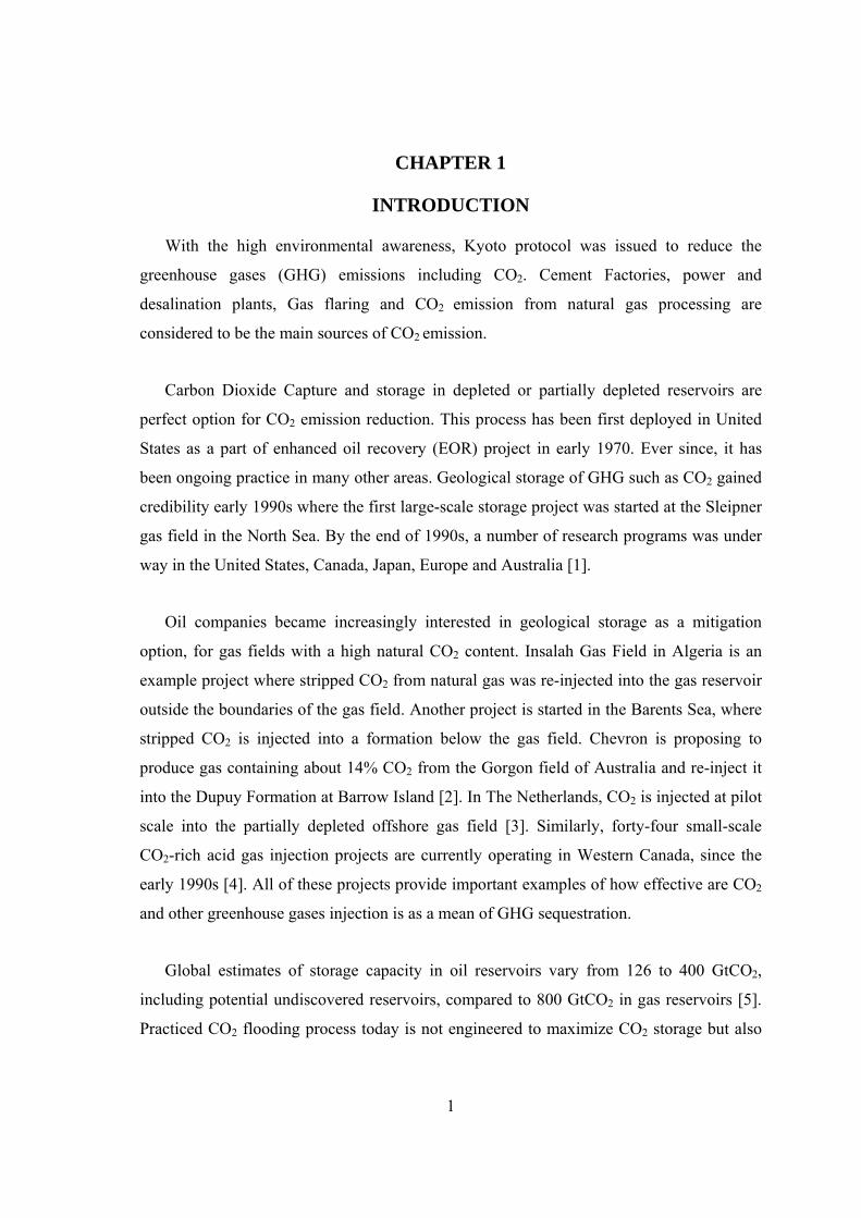
2.1 Oil recovery methods sequence in a typical oilfield [15] 4
2.2 1-D Schematic of The Dynamics CO2 Miscible Process [16] 6
2.3 Schematic of WAG miscible CO2-EOR [16] 8
2.4 Slime tube apparatus[31] 12
2.5 Schematic of the rising bubble apparatus [36] 12
2.6 Comparison of different WAG ratios in terms of the incremental oil recovery as a function of the CO2 slug size [66]....... 23
4.1 Schematic of the experimental set-up........................................................ 30
5.1 Cumulative oil recovery versus cumulative water volume injected during the water flood process on run 15 35
5.2 Effect of slug size on recovery factor of 1:1 miscible WAG displacement experiments using n-Decane-brine fluid pair……….……. 39
5.3 Effect of slug size on tertiary recovery factor of miscible 1:1 WAG displacement experiments using n-Decane-brine fluid pair…………...... 39
5.4 Effect of slug size on recovery factor of miscible 1:2 WAG displacement experiments using n-Decane-brine fluid pair…………….. 41
5.5 Effect of slug size on tertiary recovery factor of miscible 1:2 WAG displacement experiments using n-Decane -brine fluid pair…………………………………………………………. 41
5.6 Effect of miscible WAG ratio on recovery factor for 0.4 PV slug size displacement experiments using n-Decane- brine fluid pair 43
5.7 Effect of miscible WAG ratio on tertiary recovery factor for 0.4 PV slug size displacement experiments using n-Decane-brine fluid pair 45
5.8 Effect of miscible WAG ratio on recovery factor for 0.2 PV slug size displacement experiments using Saudi light crude synthetic formation brine fluid pair………………………………….…. 45
vii
5.9 Effect of miscible WAG ratio on tertiary recovery factor for 0.2 PV slug size displacement experiments using Saudi light crude-synthetic formation brine fluid pair……………...…………. 46
5.10 Effect of miscible WAG Parameters on recovery factor for n-Decane-brine fluid pair…………………………………………..... 46
5.11 Effect of miscible WAG Parameters on tertiary recovery factor for n-Decane-brine fluid pair……………………………….……. 47
5.12 CO2 Utilization Factor, tertiary recovery factor, and recovery factor of different miscible WAG parameters for n-Decane-brine fluid pair……………………………………….…… 49
5.13 Recover factor in percentage of initial oil in place for secondary and tertiary gas injection using n-Decane -brine fluid pair………………………………………………………….. 50
5.14 Tertiary recovery factor of tertiary versus secondary miscible gas injection using n-Decane-brine fluid pair…………………. 52
5.15 Effect of brine composition on n-Decane recovery factor of miscible flooding at 1:2 WAG ratio, 0.2 PV slug size…………………………………………………………. 52
5.16 Effect of brine composition on n-Decane tertiary recovery factor of miscible flooding at 1:2 WAG ratio, 0.2 PV slug size…………………………………………………………. 53
5.17 Effect of oil type on recovery factor of miscible flooding at 1:2 WAG ratio, 0.2 PV slug size……………………………………... 55
5.18 Effect of oil type on tertiary recovery factor of miscible flooding at 1:2 WAG ratio, 0.2 PV slug size……………………………. 55
5.19 Effect of core orientation on recovery factor of miscible flooding at 1:2 WAG ratio, 0.2 PV slug size using Saudi light crude-synthetic formation brine fluid pair…………………………. 57
5.20 Effect of core orientation on tertiary recovery factor of miscible flooding at 1:2 WAG ratio, 0.2 PV slug size using Saudi light crude-synthetic formation brine fluid pair………………....... 57
5.21 Effect of core length on recovery factor of miscible flooding at 1:2 WAG ratio, 0.2 PV slug size using Saudi light crude-
viii
synthetic formation brine fluid pair……………………………………... 59
5.22 Effect of core length on tertiary recovery factor of miscible flooding at 1:2 WAG ratio, 0.2 PV slug size using Saudi light crude oil- synthetic formation brine fluid pair…………………………... 59
5.23 Effect of miscible injection mode on recovery factor using n-Decane-brine fluid pair………………………………………………... 61
5.24 Effect of miscible injection mode on tertiary recovery factor using n-Decane-brine fluid pair………………………………...…. 61
5.25 CO2 Utilization Factor, tertiary recovery factor, and recovery factor of CGI and WAG injection mode for n-Decane-brine fluid pair………………………..…………….. 62
5.26 Effect of miscible injection mode on recovery factor using Saudi light crude-synthetic formation brine fluid pair on 4 ft long core………………………………………………...…... 62
5.27 Effect of miscible injection mode on tertiary recovery factor using Saudi light crude-synthetic formation brine fluid pair on 4 ft long core…………………………………...…………... 64
ix
LIST of TABLES
Table No. Page
2.1 Commonly used CO2-Oil MMP correlations 14
4.1 Physical properties of used n-Deane and aqueous solutions 27
4.2 Properties of the Saudi Crude Oils [71] 27
4.3 Minimum miscibility pressure values of the binary oil-brine
systems 28
5.1 Petrophysical properties of water flooded rock samples 34
5.2 Summery of conducted miscible gas flooding experimental runs 36
1
CHAPTER 1
INTRODUCTION
With the high environmental awareness, Kyoto protocol was issued to reduce the
greenhouse gases (GHG) emissions including CO2. Cement Factories, power and
desalination plants, Gas flaring and CO2 emission from natural gas processing are
considered to be the main sources of CO2 emission.
Carbon Dioxide Capture and storage in depleted or partially depleted reservoirs are
perfect option for CO2 emission reduction. This process has been first deployed in United
States as a part of enhanced oil recovery (EOR) project in early 1970. Ever since, it has
been ongoing practice in many other areas. Geological storage of GHG such as CO2 gained
credibility early 1990s where the first large-scale storage project was started at the Sleipner
gas field in the North Sea. By the end of 1990s, a number of research programs was under
way in the United States, Canada, Japan, Europe and Australia [1].
Oil companies became increasingly interested in geological storage as a mitigation
option, for gas fields with a high natural CO2 content. Insalah Gas Field in Algeria is an
example project where stripped CO2 from natural gas was re-injected into the gas reservoir
outside the boundaries of the gas field. Another project is started in the Barents Sea, where
stripped CO2 is injected into a formation below the gas field. Chevron is proposing to
produce gas containing about 14% CO2 from the Gorgon field of Australia and re-inject it
into the Dupuy Formation at Barrow Island [2]. In The Netherlands, CO2 is injected at pilot
scale into the partially depleted offshore gas field [3]. Similarly, forty-four small-scale
CO2-rich acid gas injection projects are currently operating in Western Canada, since the
early 1990s [4]. All of these projects provide important examples of how effective are CO2
and other greenhouse gases injection is as a mean of GHG sequestration.
Global estimates of storage capacity in oil reservoirs vary from 126 to 400 GtCO2,
including potential undiscovered reservoirs, compared to 800 GtCO2 in gas reservoirs [5].
Practiced CO2 flooding process today is not engineered to maximize CO2 storage but also
2
to maximize revenues from oil production. This requires minimizing the amount of CO2
retained in the reservoir. In the future, if storing CO2 has an economic value, co-optimizing
CO2 storage and EOR may increase capacity estimates.
In United States, there are approximately 73 CO2-EOR projects injecting up to 30
MtCO2 annually. Most of the CO2 are from natural CO2 accumulations while about 3
MtCO2 is captured from anthropogenic sources [6]. The SACROC project in Texas was the
first large-scale commercial CO2-EOR project in the world. It used anthropogenic CO2
during the years 1972-1995. Similarly, Rangely Weber project uses anthropogenic CO2
from a gas-processing plant in Wyoming. In Canada, CO2-EOR project has been started at
the Weyburn oil field. The project is expected to inject 23 MtCO2 and extend the life of the
oil field by 25 years [7,8]. CO2-EOR projects are under way nowadays in the offshore
North Sea reservoirs. Different projects are also currently under way in Trinidad, Turkey
and Brazil [9].
Many CO2 injection schemes have been suggested, including continuous gas injection
(CGI) or water alternating gas (WAG) injection in miscible and immiscible injection
modes. The displacement mechanisms range from oil swelling and viscosity reduction for
immiscible CO2 injection (below minimum miscibility pressure (MMP)) to completely
miscible displacement in high-pressure applications (above MMP). Portion of injected gas
returns with the produced oil. Therefore, it is usually re-injected into the reservoir to
minimize operating costs [10].
The main objective of this study is to evaluate the performance of miscible CO2
flooding at different conditions. To fulfill this objective extensive laboratory tests were
conducted on 2 and 4 ft long sandstone cores using low and high salinity brine solutions as
aqueous phase and three different oleic phases (n-Decane, Saudi-light and Saudi-medium
crudes). Injection scheme ("CGI" versus "WAG"), WAG ratio, slug size, oil types, core
orientation and core length were investigated. In addition, miscible WAG flooding as a
secondary process was investigated and its efficiency was compared to the conventional
tertiary miscible gas flooding.
3
CHAPTER 2
LITERATURE REVIEW
Enhanced Oil Recovery (EOR) essentially defined as the oil recovery by any method
beyond the primary reservoir drive. These include pressure maintenance, water injection or
other kind of techniques. Usually 5 to 40% of original oil in place is recovered by primary
recovery methods [11]. Additional 10 to 20% of oil in place is produced by secondary
methods such as water flooding [12]. Tertiary recovery methods, such as CO2 flooding,
have been practiced with incremental oil recovery of 7 to 23% of the original oil in place
[13, 10], (see Figure 2.1). All the mentioned numbers depends on the properties of oil and
the characteristics of the reservoir rocks. CO2 could also be injected into depleted gas
reservoirs to increase reservoir pressure and to enhance gas recovery although high
percentage of original gas in place can be recovered primarily.
The appreciable decline in hydrocarbon reservoirs discovery and the increasing demand
for oil and gas led the companies to explore the different EOR methods such as chemical,
thermal and gas flooding. Carbon dioxide is an available gas and it becomes more attractive
choice with the high environmental awareness of the harmful effects of GHG. Currently
there are 75 CO2-EOR projects world wide producing 194 million barrel per day most of
which in united states [14].
When injected into the reservoir CO2 interacts chemically and physically with the
reservoir rock and the contained fluids, creating favorable conditions that improve oil
recovery. These conditions include the following [14]:
1. Reducing the interfacial tension between oil and the reservoir rock that inhibit
oil flow through the pores of the reservoir.
2. The expansion of oil volume and the subsequent reduction of its viscosity.
3. The development of complex phase changes in the oil that increases its fluidity.
4. The maintenance of favorable mobility characteristics for oil and CO2 to
improve the sweep efficiency.
4
Figure 2.1: Oil recovery methods sequence in a typical oilfield [15].
5
Two processes have been performed for CO2-EOR process. These are miscible and
immiscible displacements. The applicability of each process depends on the reservoir
conditions. CO2 -EOR processes are also distinguished as CGI or WAG injection method.
In WAG process, CO2 is injected first to cause oil swelling and improve its fluidity.
Another slug of water is then injected to displace the oil bank towards the production well.
The concurrent flow of water and CO2 results in the reduction of the mobility of each
phase, reducing the occurrences of viscous fingering. In addition, the presence of water in
the reservoir improves oil recovery, as it forms a fast diffusion path for CO2 to reach oil
trapped in the pores of the reservoir rock.
Another method of CO2 injection is the immiscible gravity stable gas injection (GSGI)
where CO2 is injected in the crest at the gas zone, forcing the oil to move downwards
towards the producing wells. WAG has an advantage over GSGI in that it can be performed
on a small scale, while in general; GSGI is applied in the whole oilfield. Hence GSGI
projects are likely to recover more oil and store larger CO2 volumes [16, 17].
2.1 Miscible CO2 Flooding
Under favorable crude oil composition and reservoir pressure and temperature, CO2 can
be miscible with oil, forming a single-phase liquid. As a result, the volume of oil swells and
its viscosity and surface tension is reduced, improving the ability of the oil to flow and
increasing oil recovery. CO2 is not miscible with oil at first contact but miscibility develops
dynamically through composition changes when the CO2 gradually interacts with oil. This
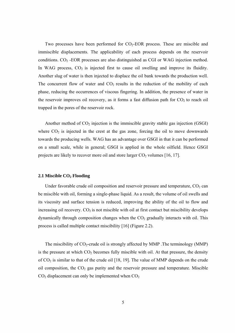
process is called multiple contact miscibility [16] (Figure 2.2).
The miscibility of CO2-crude oil is strongly affected by MMP .The terminology (MMP)
is the pressure at which CO2 becomes fully miscible with oil. At that pressure, the density
of CO2 is similar to that of the crude oil [18, 19]. The value of MMP depends on the crude
oil composition, the CO2 gas purity and the reservoir pressure and temperature. Miscible
CO2 displacement can only be implemented when CO2
6
Figure 2.2: 1-D Schematic of The Dynamics CO2 Miscible Process [16].
7
is injected at a pressure higher than the MMP, which must be lower than the reservoir
pressure. MMP can nowadays be measured experimentally or predicted empirically and
through thermodynamic modeling with a very good accuracy. A review of the current
knowledge on the matter is presented in references [19, 20].
For miscible CO2-EOR operations, oil reservoirs may need to meet specific criteria [21,
22, and 23]. Among these are reservoir depths, which must be more than 2500 ft to achieve
miscibility because with shallower depths low miscibility pressure cannot be attained
without fracturing the formation. Miscibility pressure usually increases with decreasing oil
gravity. Therefore, Injection of miscible fluids is a good option of Low and medium
viscosity oils (0.3 - 6 cp).
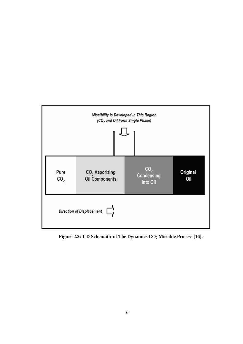
To prevent the occurrences of unstable flow and to reduce the amount of CO2 needed
for the process, CO2 is typically injected into the reservoir alternately with water. WAG
process was initially proposed to increase the sweep efficiency in gas flooding process.
Generally WAG process is a combination of both traditional water flooding and gas
injection techniques as shown in Figure 2.3. In this process, equal volumes of CO2 and
water slugs are injected in cycles at constant or different gas/water ratio, to improve sweep
efficiencies of water flooding and miscible gas floods. The oil recovery improvement in
WAG process is due to the mass transfer between the gas intermediate components and
reservoir oil to develop miscible front. Expected increase in oil recovery by miscible WAG
injection process presented in the literature are 10-15% in the Permian basin compared to 6
to 12% incremental recovery in some North Sea reservoirs using immiscible CO2 flooding
[16].
Data from 10 miscible displacement projects in the Permian basin indicate that the net
injection of CO2 into an oilfield is on average 164 m3 per barrel (bbl) of incremental oil.
The evaluation of large number of US projects suggest that the average incremental
recovery of oil lies in the range of 4-12% OOIP while the net volume of CO2 injected is in
the range of 10-45% of the OOIP. The highest oil recovery efficiencies are associated
8
Figure 2.3: Schematic of a WAG miscible CO2-EOR [16].
9
the tapered WAG injection process where the ratio of injected water to CO2 changes with
time, starting with larger CO2 slugs that decrease in size with time [16].
General problems with miscible displacement that may cause failure can be
summarized into the following:
• Insufficient reservoir geology and petrophysical information before starting a
project.
• Reduction of reservoir pressure due to reduced injectivity caused by asphaltene
deposition that may result in loss of miscibility and hence reduction of recovery.
• Failure of water pipelines and wells due to scale formation.
• Corrosion promoted by the carbonic acid formed by CO2 dissolution in water.
2.1.1 Minimum Miscibility Pressure (MMP)
MMP is an important concept associated with the description of miscible gas injection
processes. MMP is defined as the lowest pressure at which a crude oil and a solvent
develop miscibility dynamically. At this pressure, the injected gas and the initial oil in
place become multi contact miscible, and the displacement process becomes very efficient.
If the displacement process is represented as a one dimensional, two-phase, dispersion-free
flow, then at the MMP, the displacement is piston-like, and the oil recovery is 100% at 1
pore volume of gas injected.
The MMP is an important parameter in the design of a miscible gas injection project.
The rationale behind the determination of MMP for a particular miscible gas injection
project is that there is a trade off between achieving high oil recovery and reducing
production costs. If the injection pressure is too low, the displacement would still be two-
phase immiscible, and therefore the local displacement efficiency would be below the
desired level. If the pressure is too high, although the displacement would become multi
contact miscible, and the oil recovery would reach the desired level, the cost of pressurizing
the injected gas would be larger than necessary. Hence an optimal pressure has to be found,
and that pressure is MMP. A closely related concept is the minimum miscibility enrichment
(MME). It is the enrichment level of a particular component or group of components in a
10
multi component injection gas for a given displacement pressure that causes the
displacement to become multi contact miscible. Conceptually the MMP and MME are the
same; they describe the same physical mechanism, one from the point of view of varying
pressure to achieve miscibility, the other from the point of view of varying injection gas
composition [24, 25].
Accurate determination of MMP or MME for a miscible gas injection process is of a
considerable interest to the petroleum industry. Traditionally the MMP or MME is
determined either experimentally or mathematically [24, 25].
2.1.1.1 Experimental Methods
There are several ways to measure MMP experimentally. The slim tube test is one of
the most widely used techniques and is accepted as a standard mean to measure MMP in
the petroleum industry. In a typical test, a slim tube made of stainless steel is packed with a
porous material such as glass beads or sand. The tube is initially saturated with oil. Gas is
injected at the inlet of the tube to displace oil at the desired test temperature and pressure.
Effluent from the tube is collected and measured to obtain the recovery curve. Sometimes a
visual cell is mounted downstream of the tube to allow visual inspection of the
development of miscibility. The recovery data are plotted against the displacement
pressures under which the tests are performed, and the recovery curve is used to infer the
MMP. The criteria used by various investigators to determine the MMP from the oil
recovery curve are different. A commonly used injection volume is 1.2 pore volumes.
Fixed recovery levels defining MMP range from 90% to 95% [26, 27].in addition, recovery
values of 85% or 90% at breakthrough accompanied by 95% to 98% ultimate recovery have
been used [28]. The bend in the recovery curve or point of maximum curvature is also used
to define the minimum miscibility pressure [29, 30].
The point of maximum curvature occurs near the intersection of the extrapolated
asymptotes of the low- and high-recovery regions. The pressure at which the recovery
curve levels of is taken to be the MMP. Flock et al. [30] argued that the point of maximum
curvature on the recovery curve is probably a better indication of miscibility. However,
slim tube tests are expensive and time-consuming. The slim tube displacement test is often
11
referred to as the “industry standard” for determining MMP. Unfortunately; there is neither
a standard design, nor a standard operating procedure, nor a standard set of criteria for
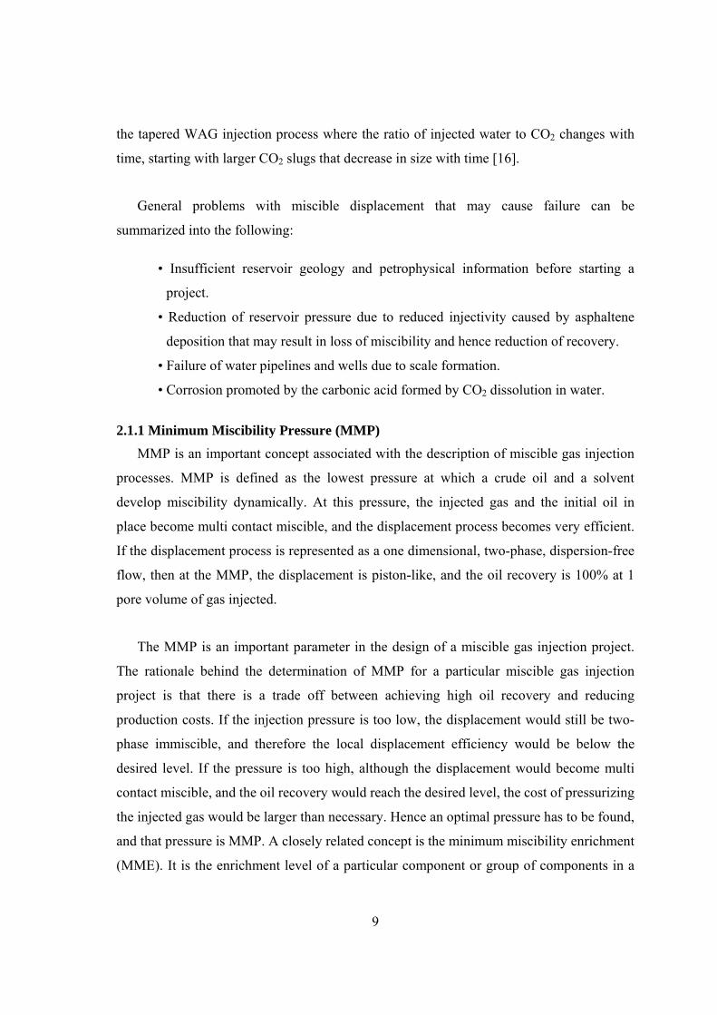
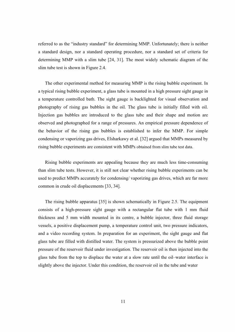
determining MMP with a slim tube [24, 31]. The most widely schematic diagram of the
slim tube test is shown in Figure 2.4.
The other experimental method for measuring MMP is the rising bubble experiment. In
a typical rising bubble experiment, a glass tube is mounted in a high pressure sight gauge in
a temperature controlled bath. The sight gauge is backlighted for visual observation and
photography of rising gas bubbles in the oil. The glass tube is initially filled with oil.
Injection gas bubbles are introduced to the glass tube and their shape and motion are
observed and photographed for a range of pressures. An empirical pressure dependence of
the behavior of the rising gas bubbles is established to infer the MMP. For simple
condensing or vaporizing gas drives, Elsharkawy et al. [32] argued that MMPs measured by
rising bubble experiments are consistent with MMPs obtained from slim tube test data.
Rising bubble experiments are appealing because they are much less time-consuming
than slim tube tests. However, it is still not clear whether rising bubble experiments can be
used to predict MMPs accurately for condensing/ vaporizing gas drives, which are far more
common in crude oil displacements [33, 34].
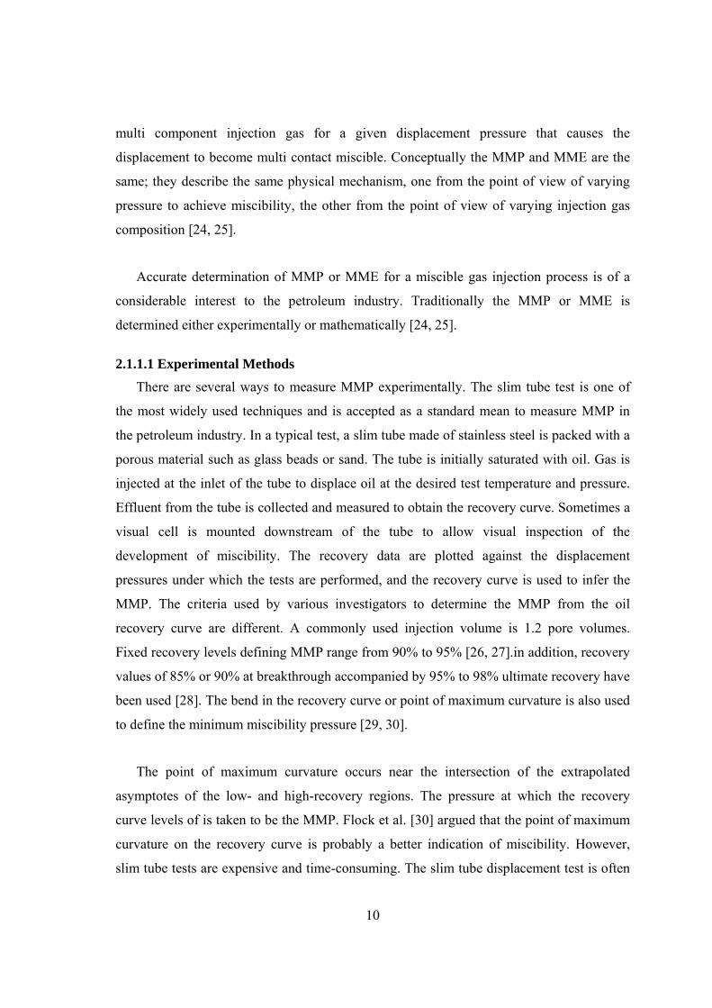
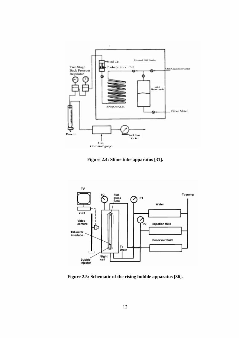
The rising bubble apparatus [35] is shown schematically in Figure 2.5. The equipment
consists of a high-pressure sight gauge with a rectangular flat tube with 1 mm fluid
thickness and 5 mm width mounted in its centre, a bubble injector, three fluid storage
vessels, a positive displacement pump, a temperature control unit, two pressure indicators,
and a video recording system. In preparation for an experiment, the sight gauge and flat
glass tube are filled with distilled water. The system is pressurized above the bubble point
pressure of the reservoir fluid under investigation. The reservoir oil is then injected into the
glass tube from the top to displace the water at a slow rate until the oil–water interface is
slightly above the injector. Under this condition, the reservoir oil in the tube and water
12
Figure 2.4: Slime tube apparatus [31].
Figure 2.5: Schematic of the rising bubble apparatus [36].
13
around the tube are at the same pressure. A CO2 bubble is launched into the water just
beneath the oil–water interface. As the bubble rises through the oil–water interface and then
the reservoir oil, its shape and motion are recorded. The movement of the bubble through
the oil column mimics the forward contact between CO2 and oil during the injection of a
CO2 slug through the reservoir. After one or two bubbles are injected into an oil sample,
water is injected from the bottom to displace the used oil. Then, fresh oil is injected from
the top to fill the glass tube for further rising bubble tests. For a gas–oil pair, rising bubble
experiments are repeated over a range of pressures. The MMP is defined as the pressure at
which the bubble and the oil showed multiple-contact miscibility [36].
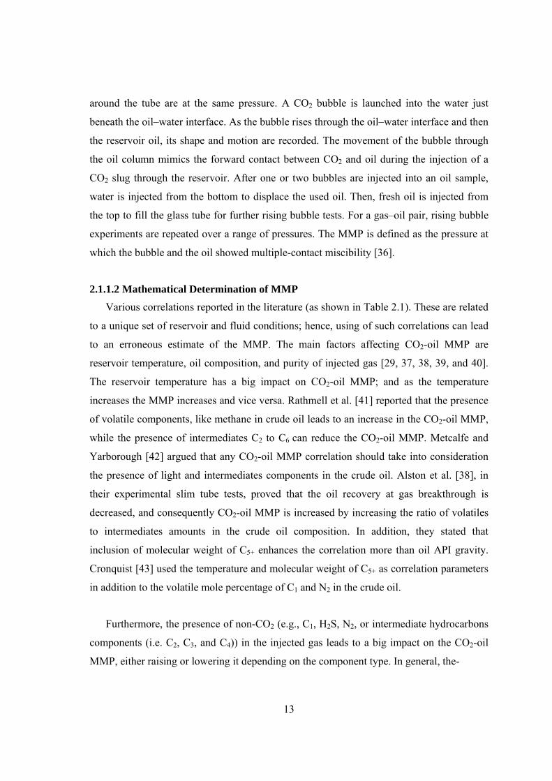
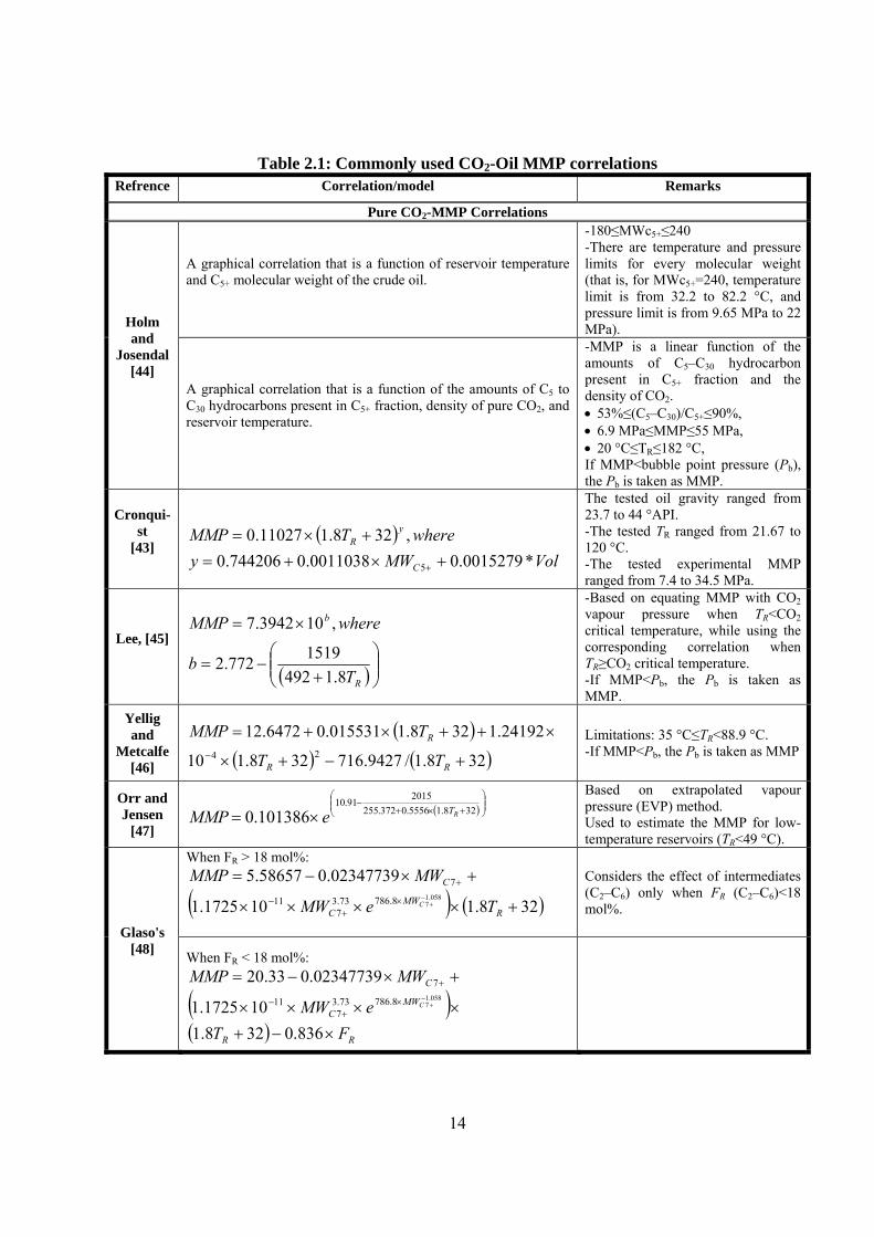
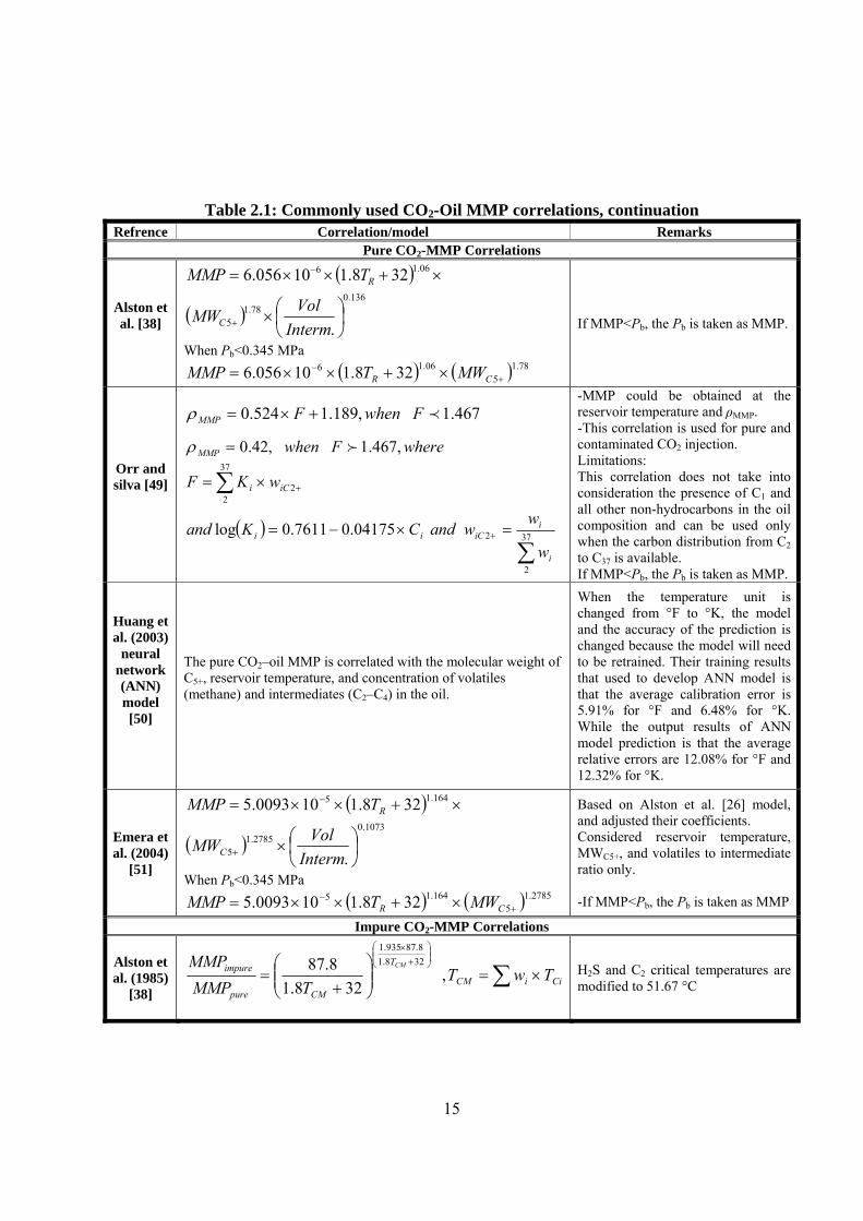
2.1.1.2 Mathematical Determination of MMP
Various correlations reported in the literature (as shown in Table 2.1). These are related
to a unique set of reservoir and fluid conditions; hence, using of such correlations can lead
to an erroneous estimate of the MMP. The main factors affecting CO2-oil MMP are
reservoir temperature, oil composition, and purity of injected gas [29, 37, 38, 39, and 40].
The reservoir temperature has a big impact on CO2-oil MMP; and as the temperature
increases the MMP increases and vice versa. Rathmell et al. [41] reported that the presence
of volatile components, like methane in crude oil leads to an increase in the CO2-oil MMP,
while the presence of intermediates C2 to C6 can reduce the CO2-oil MMP. Metcalfe and
Yarborough [42] argued that any CO2-oil MMP correlation should take into consideration
the presence of light and intermediates components in the crude oil. Alston et al. [38], in
their experimental slim tube tests, proved that the oil recovery at gas breakthrough is
decreased, and consequently CO2-oil MMP is increased by increasing the ratio of volatiles
to intermediates amounts in the crude oil composition. In addition, they stated that
inclusion of molecular weight of C5+ enhances the correlation more than oil API gravity.
Cronquist [43] used the temperature and molecular weight of C5+ as correlation parameters
in addition to the volatile mole percentage of C1 and N2 in the crude oil.
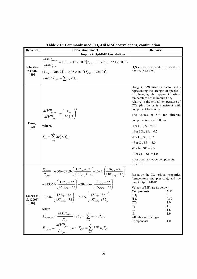
Furthermore, the presence of non-CO2 (e.g., C1, H2S, N2, or intermediate hydrocarbons
components (i.e. C2, C3, and C4)) in the injected gas leads to a big impact on the CO2-oil
MMP, either raising or lowering it depending on the component type. In general, the-
14
Table 2.1: Commonly used CO2-Oil MMP correlations Refrence Correlation/model Remarks
Pure CO2-MMP Correlations
A graphical correlation that is a function of reservoir temperature and C5+ molecular weight of the crude oil.
-180≤MWc5+≤240 -There are temperature and pressure limits for every molecular weight (that is, for MWc5+=240, temperature limit is from 32.2 to 82.2 °C, and pressure limit is from 9.65 MPa to 22 MPa). Holm
and Josendal
[44] A graphical correlation that is a function of the amounts of C5 to
C30 hydrocarbons present in C5+ fraction, density of pure CO2, and reservoir temperature.
-MMP is a linear function of the amounts of C5–C30 hydrocarbon present in C5+ fraction and the density of CO2. • 53%≤(C5–C30)/C5+≤90%, • 6.9 MPa≤MMP≤55 MPa, • 20 °C≤TR≤182 °C, If MMP<bubble point pressure (Pb), the Pb is taken as MMP.
Cronqui-st
[43]
( )VolMWy
whereTMMP
C
yR
*0015279.00011038.0744206.0,328.111027.0
5 +×+=+×=
+
The tested oil gravity ranged from 23.7 to 44 °API. -The tested TR ranged from 21.67 to 120 °C. -The tested experimental MMP ranged from 7.4 to 34.5 MPa.
Lee, [45]
( )⎟⎟⎠
⎞⎜⎜⎝
⎛+
−=
×=
R
b
Tb
whereMMP
8.14921519772.2
,103942.7
-Based on equating MMP with CO2 vapour pressure when TR<CO2 critical temperature, while using the corresponding correlation when TR≥CO2 critical temperature. -If MMP<Pb, the Pb is taken as MMP.
Yellig and
Metcalfe [46]
( )( ) ( )328.1/9427.716328.110
24192.1328.1015531.06472.1224 +−+×
×++×+=−
RR
R
TT
TMMP
Limitations: 35 °C≤TR<88.9 °C. -If MMP<Pb, the Pb is taken as MMP
Orr and Jensen
[47] ( ) ⎟⎟
⎠
⎞⎜⎜⎝
⎛+×+
−
×= 328.15556.0372.255201591.10
101386.0 RTeMMP
Based on extrapolated vapour pressure (EVP) method. Used to estimate the MMP for low-temperature reservoirs (TR<49 °C).
When FR > 18 mol%:
( ) ( )328.1101725.1
02347739.058657.5058.1
78.78673.37
11
7
+××××
+×−=−
+×+
−
+
RMW
C
C
TeMW
MWMMPC
Considers the effect of intermediates (C2–C6) only when FR (C2–C6)<18 mol%.
Glaso's [48]
When FR < 18 mol%:
( )( ) RR
MWC
C
FTeMW
MWMMPC
×−+××××
+×−=−
+×+
−
+
836.0328.1101725.1
02347739.033.20058.1
78.78673.37
11
7
15
Table 2.1: Commonly used CO2-Oil MMP correlations, continuation Refrence Correlation/model Remarks
Pure CO2-MMP Correlations
Alston et al. [38]
( )
( )136.0
78.15
06.16
.
328.110056.6
⎟⎠⎞
⎜⎝⎛×
×+××=
+
−
IntermVolMW
TMMP
C
R
When Pb<0.345 MPa ( ) ( ) 78.1
506.16 328.110056.6 +
− ×+××= CR MWTMMP
If MMP<Pb, the Pb is taken as MMP.
Orr and silva [49]
467.1,189.1524.0 pFwhenFMMP +×=ρ
whereFwhenMMP ,467.1,42.0 f=ρ
( )∑
∑
=×−=
×=
+
+
37
2
2
37
22
04175.07611.0logi
iiCii
iCi
w
wwandCKand
wKF
-MMP could be obtained at the reservoir temperature and ρMMP. -This correlation is used for pure and contaminated CO2 injection. Limitations: This correlation does not take into consideration the presence of C1 and all other non-hydrocarbons in the oil composition and can be used only when the carbon distribution from C2 to C37 is available. If MMP<Pb, the Pb is taken as MMP.
Huang et al. (2003)
neural network (ANN) model [50]
The pure CO2–oil MMP is correlated with the molecular weight of C5+, reservoir temperature, and concentration of volatiles (methane) and intermediates (C2–C4) in the oil.
When the temperature unit is changed from °F to °K, the model and the accuracy of the prediction is changed because the model will need to be retrained. Their training results that used to develop ANN model is that the average calibration error is 5.91% for °F and 6.48% for °K. While the output results of ANN model prediction is that the average relative errors are 12.08% for °F and 12.32% for °K.
Emera et al. (2004)
[51]
( )
( )1073.0
2785.15
164.15
.
328.1100093.5
⎟⎠⎞
⎜⎝⎛×
×+××=
+
−
IntermVolMW
TMMP
C
R
When Pb<0.345 MPa ( ) ( ) 2785.1
5164.15 328.1100093.5 +
− ×+××= CR MWTMMP
Based on Alston et al. [26] model, and adjusted their coefficients. Considered reservoir temperature, MWC5+, and volatiles to intermediate ratio only. -If MMP<Pb, the Pb is taken as MMP
Impure CO2-MMP Correlations
Alston et al. (1985)
[38] ∑ ×=⎟⎟
⎠
⎞⎜⎜⎝
⎛+
=⎟⎟⎠
⎞⎜⎜⎝
⎛+
×
CiiCM
T
CMpure
impure TwTTMMP
MMP CM
,328.1
8.87 328.18.87935.1
H2S and C2 critical temperatures are modified to 51.67 °C
16
Table 2.1: Commonly used CO2-Oil MMP correlations, continuation Refrence Correlation/model Remarks
Impure CO2-MMP Correlations
Sebastia-n et al.
[29]
( )
( ) ( )∑ ×=
−×−−
××+−×−=
−
−−
CiiCM
CMCM
CMpure
impure
TxTwherTT
TMMPMMP
:,2.3041035.22.304
1051.22.3041013.20.1
372
42
H2S critical temperature is modified 325 °K (51.67 °C)
Dong, [52]
4
2.304⎟⎠⎞
⎜⎝⎛= ac
pure
impure TMMPMMP
Where,
∑=
×=n
iCiiac TSFT
1
Dong (1999) used a factor (SFi) representing the strength of species I in changing the apparent critical temperature of the impure CO2 relative to the critical temperature of CO2 (this factor is consistent with component K-values).
The values of SFi for different
components are as follows:
-For H2S, SFi = 0.7
- For SO2, SFi = 0.5
-For C1, SFi = 2.5
- For O2, SFi = 5.0
-For N2, SFi = 7.5
- For CO2, SFi = 1.0
- For other non-CO2 components, SFi = 1.0
Emera et al. (2005)
[40]
6
,
5
,
4
,
3
,
2
,,,
,
328.1328.1009.18
328.1328.146.98
328.1328.1366.208
328.1328.1363.213
328.1328.15.109
328.1328.169.29606.6
22
22
22
⎟⎟⎠
⎞⎜⎜⎝
⎛
++
×+⎟⎟⎠
⎞⎜⎜⎝
⎛
++
×−
⎟⎟⎠
⎞⎜⎜⎝
⎛
++
×+⎟⎟⎠
⎞⎜⎜⎝
⎛
++
×−
⎟⎟⎠
⎞⎜⎜⎝
⎛
++
×+⎟⎟⎠
⎞⎜⎜⎝
⎛
++
×−=
COC
CW
COC
CW
COC
CW
COC
CW
COC
CW
COC
CW
purer
impurer
TT
TT
TT
TT
TT
TT
PP
where
CW
impureimpurer P
MMPP =, , ∑
=
×=n
iCW PciwiP
1
,
pureC
purepurer P
MMPP
,, = , and ∑
=
=n
iCiiiCW TwMFT
1
Based on the CO2 critical properties (temperature and pressure), and the pure CO2-oil MMP.
Values of MFi are as below: Components MFi SO2 0.3 H2S 0.59 CO2 1.0 C2 1.1 C1 1.6 N2 1.9 All other injected gas Components 1.0
17
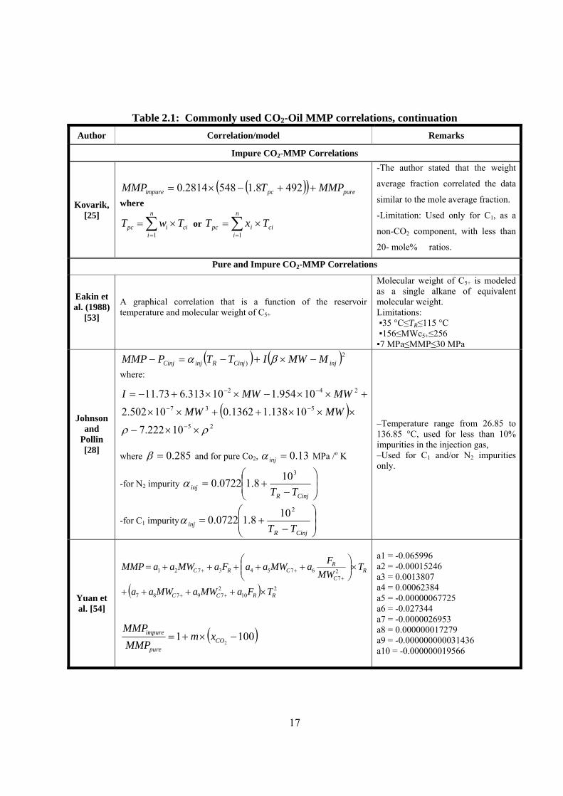
Table 2.1: Commonly used CO2-Oil MMP correlations, continuation
Author Correlation/model Remarks
Impure CO2-MMP Correlations
Kovarik, [25]
( )( ) purepcimpure MMPTMMP ++−×= 4928.15482814.0 where
∑=
×=n
iciipc TwT
1 or ∑
=
×=n
iciipc TxT
1
-The author stated that the weight
average fraction correlated the data
similar to the mole average fraction.
-Limitation: Used only for C1, as a
non-CO2 component, with less than
20- mole% ratios.
Pure and Impure CO2-MMP Correlations
Eakin et al. (1988)
[53]
A graphical correlation that is a function of the reservoir temperature and molecular weight of C5+
Molecular weight of C5+ is modeled as a single alkane of equivalent molecular weight. Limitations: ▪35 °C≤TR≤115 °C ▪156≤MWc5+≤256 ▪7 MPa≤MMP≤30 MPa
Johnson and
Pollin [28]
( ) ( )2) injCinjRinjCinj MMWITTPMMP −×+−=− βα where:
( )25
537
242
10222.710138.11362.010502.2
10954.110313.673.11
ρρ ××−
×××++××
+××−××+−=
−
−−
−−
MWMWMWMWI
where 285.0=β and for pure Co2, 13.0=injα MPa /o K
-for N2 impurity ⎟⎟⎠
⎞⎜⎜⎝
⎛
−+=
CinjRinj TT
3108.10722.0α
-for C1 impurity ⎟⎟⎠
⎞⎜⎜⎝
⎛
−+=
CinjRinj TT
2108.10722.0α
–Temperature range from 26.85 to 136.85 °C, used for less than 10% impurities in the injection gas, –Used for C1 and/or N2 impurities only.
Yuan et al. [54]
( ) 210
279787
27
67543721
RRCC
RC
RCRC
TFaMWaMWaa
TMW
FaMWaaFaMWaaMMP
×++++
×⎟⎟⎠
⎞⎜⎜⎝
⎛+++++=
++
+++
( )10012−×+= CO
pure
impure xmMMPMMP
a1 = -0.065996 a2 = -0.00015246 a3 = 0.0013807 a4 = 0.00062384 a5 = -0.00000067725 a6 = -0.027344 a7 = -0.0000026953 a8 = 0.000000017279 a9 = -0.000000000031436 a10 = -0.000000019566
18
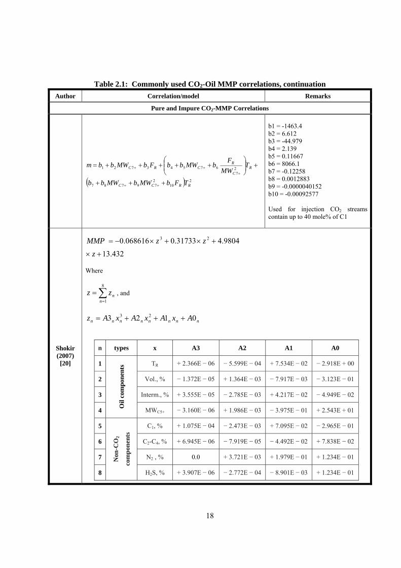
Table 2.1: Commonly used CO2-Oil MMP correlations, continuation
Author Correlation/model Remarks
Pure and Impure CO2-MMP Correlations
( ) 210
279787
27
67543721
RRCC
RC
RCRC
TFbMWbMWbb
TMW
FbMWbbFbMWbbm
+++
+⎟⎟⎠
⎞⎜⎜⎝
⎛+++++=
++
+++
b1 = -1463.4 b2 = 6.612 b3 = -44.979 b4 = 2.139 b5 = 0.11667 b6 = 8066.1 b7 = -0.12258 b8 = 0.0012883 b9 = -0.0000040152 b10 = -0.00092577 Used for injection CO2 streams contain up to 40 mole% of C1
Shokir (2007) [20]
432.13
9804.431733.0068616.0 23
+×
+×+×−=
z
zzMMP
Where
∑=
=8
1nnzz , and
nnnnnnnn AxAxAxAz 0123 23 +++=
n types x A3 A2 A1 A0
1 TR + 2.366E − 06 − 5.599E − 04 + 7.534E − 02 − 2.918E + 00
2 Vol., % − 1.372E − 05 + 1.364E − 03 − 7.917E − 03 − 3.123E − 01
3 Interm., % + 3.555E − 05 − 2.785E − 03 + 4.217E − 02 − 4.949E − 02
4 Oil
com
pone
nts
MWC5+ − 3.160E − 06 + 1.986E − 03 − 3.975E − 01 + 2.543E + 01
5 C1, % + 1.075E − 04 − 2.473E − 03 + 7.095E − 02 − 2.965E − 01
6 C2-C4, % + 6.945E − 06 − 7.919E − 05 − 4.492E − 02 + 7.838E − 02
7 N2 , % 0.0 + 3.721E − 03 + 1.979E − 01 + 1.234E − 01
8
Non
-CO
2
com
pone
nts
H2S, % + 3.907E − 06 − 2.772E − 04 − 8.901E − 03 + 1.234E − 01
19
presence of H2S, or intermediate hydrocarbon components in the injected gas decreases the
CO2-oil MMP, while the presence of C1 or N2 in the injected gas substantially increases the
CO2-oil MMP. N2 from flue gas and C1 from re-injected CO2 are the large possible
contaminants to CO2 and recycled CO2. The separation of such components from the
injected gas is difficult and costly. The current trend is to use the flue gas stream as it is, if
such impurities are below certain optimum level in the injected gas stream. Therefore, the
developed model using the ACE algorithm, was designed to reach the optimal regression
between the pure or impure CO2-oil MMP and the reservoir temperature, mole percentage
of oil components (volatiles (C1 and N2), intermediate components (C2-C4), and H2S and
CO2)), MWC5+, and mole percentage of the non-CO2 components (C1, N2, H2S, and C2-C4)
in the injected CO2.
2.2 Immiscible CO2 Displacement Method
Immiscible CO2 displacement process can enhance oil recovery especially in low
pressure reservoirs or in case of recovering heavy oils. In immiscible displacement, CO2 is
injected to raise and maintain reservoir pressure. In addition, although not miscible with the
reservoir fluids, CO2 can partially dissolve in oil causing some swelling and viscosity
reduction by a factor of 10. Immiscible CO2 flooding is practiced in limited number of
projects to raise reservoir pressure when rock permeability is too low or geologic
conditions do not favor the use of usually practiced water flooding. In this process, CO2 is
typically injected in GSGI mode and to less extent in WAG mode. CO2-GSGI is typically
injected at slow rates at the reservoir crest to create an artificial gas cap, displacing oil
downwards towards the production wells. This process may not be effective when applied
after significant water flooding or when water present within the reservoir [16].
The immiscible displacement process has limited applications so far, due to the
unfeasible economics. In immiscible project significant amounts of CO2 are injected in the
whole reservoir, limiting the opportunities for small-scale implementation to recover
incremental oil at a very slow pace. However, immiscible displacement projects can store
larger volumes of CO2 than miscible ones making this process more attractive for CO2
capture and storage.
20
Experience shows that the conditions that are favor in the immiscible displacement
include [16]:
1. High vertical reservoir permeability.
2. Presence of substantial amount of oil to form a thick oil column.
3. Steep dipping and good lateral and vertical communication through the
reservoir.
4. Absence of fractures that may reduce sweep efficiency.
An example of large immiscible displacement process is the Bati Raman oilfield, in
southeast Turkey. The field contains heavy oil with very low gravity. CO2 displacement oil
recovery was 6.5% of OOIP compared to 1.5% using traditional oil recovery techniques
[16]. A number of immiscible displacement pilot projects were initiated in the USA.
However full commercial projects were not successful despite the promising results from
the pilot studies [55]. Currently, one small-scale immiscible project is present in the USA,
and 5 pilot projects in Trinidad [16, 55]. A number of immiscible displacement projects
were also conducted in Hungary, using natural CO2 reserve with overall CO2 utilization of
380 m3/barrel of oil. Despite the small experience in immiscible displacement, it has been
estimated that the utilization of CO2 is within the range 280-400 m3 of CO2 per barrel of
incremental oil [16, 55]. It is expected that the process may yield approximately up to 20%
of OOIP [24, 56].
2.3 Water Alternating Gas Injection (WAG) Process
Early Laboratory models conducted showed that simultaneous water/gas injection had
sweep efficiency as high as 90%, compared to 60% for gas injection alone [57]. However,
completion cost, operations complexity, and gravity segregation indicated that it is an
impractical to minimize mobility. Therefore, a CO2 slug followed by WAG has been
adopted. The planned WAG ratios of 0.5:4 in frequencies of 0.1 to 2% PV slugs of each
fluid cause water-saturation to increase during the water cycles and to decrease during the-
gas cycle[58]. Claudle and Dyes [57] suggested simultaneous injection of water and gas to
improve mobility control, however, the field reviews show that they are usually injected
21
separately [59]. There are important technical factors affecting WAG performance. These
were identified as heterogeneity [60], wettability [18], reservoir fluids properties [61],
miscibility conditions [60, 61], injection techniques [60, 61], WAG parameters [60, 61],
physical dispersion [62], and flow geometry [60, 61] with most of the research work,
conducted on either core flooding [57, 60] or numerical simulation [58, 61], sometimes
alongside field trials.
A number of different WAG schemes are used to optimize recovery. Unocal patented a
process called Hybrid WAG in which a large fraction of the pore volume of CO2 is injected
continuously, followed by the remaining fraction divided into 1:1 WAG ratios [63]. Shell
developed a similar process called Denver Unit WAG (DUWAG14) by comparing
continuous injection and WAG processes
The major design issues to be considered for WAG injection process are WAG ratio,
injection rate, ultimate CO2 slug size, reservoir characteristic and heterogeneity, rock and
fluid characteristics, and injection pattern. In this thesis; I will concentrate on the literature
discussing the parameters investigated in our laboratory so far such as WAG ratio and CO2
slug size.
2.3.1 WAG Ratio
An optimum WAG ratio is a major design parameter that has a significant effect on
operation and economics of a CO2 flood. WAG ratio is defined as the ratio of injected
water volume to CO2 volume in each cycle. WAG ratios may be expressed in terms of
barrels of water injected at reservoir conditions or in terms of the time of injection [64].
The WAG ratio is controlled by the gas availability as well as the reservoir rock wettability
[65]. To maximize the net present value of CO2 flood, WAG ratio should be increased
gradually after the optimum gas production is reached [60]. The gradual increase of
injected water (a decrease in the WAG ratio) results in increased mobility control and a
constant produced gas profile. Laboratory studies [65] on WAG ratios showed that tertiary
CO2 floods have maximum recoveries at WAG ratio of about 1:1 in floods dominated by
viscous fingering whereas continuous gas injection (0:1 WAG ratio) showed optimum
recovery in floods dominated by gravity tonguing. Hence, continuous gas injection is
22
recommended for secondary as well as tertiary floods in water-wet rocks, whereas 1:1
WAG is recommended for partially oil-wet rocks. An analytical model indicated that the
higher the WAG ratio, the lower the recovery but the better the mobility ratio. This
suggests the importance of determining the optimum WAG ratio for WAG injection
process [57, 60].
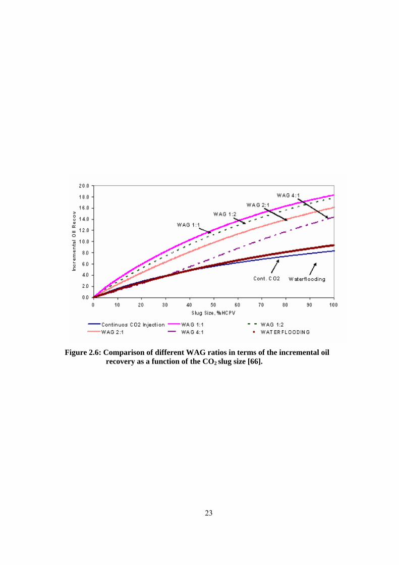
Simulation studies for Wasson Field, West Texas were carried out to investigate the
important design issues for WAG process (WAG ratio and slug size). WAG injections at
four different WAG ratios (1:1, 1:2, 2:1, and 4:1) were performed. The runs evaluated CO2
slug sizes up to 100% hydrocarbon pore volume (HCPV). Results indicate that injecting a
100% HCPV slug of CO2 with a 1:1 and 1:2 WAG ratio would yield the maximum
incremental oil recovery [66] (See figure 2.6).
In practice all patterns may start at the same WAG ratio. Later, as the CO2 production
increases due to poor volumetric sweep efficiency, the WAG ratio is usually increased on a
pattern-by-pattern basis starting with the highest GOR patterns [33].
2.3.2 Slug Size
Slug size refers to the cumulative CO2 volume injected during a CO2 flood. The slug
volume is usually expressed as a percentage of rock pore volume or HCPV [64]. Optimum
CO2 slug size is critical in a proper design of miscible flooding [56]. Generally as more
CO2 volume injected, greater incremental oil is recovered. However, a large CO2 slug size
decreases the profitability of the project.
The optimum CO2 slug size for a particular project depends on economical factors such as
crude price, CO2 cost, and the amount and timing of the incremental recovery. The
economical optimization process is conducted by repeated simulation runs until optimum
design parameters are achieved [67]. The ultimate CO2 slug size can be determined after
the start of project, when more information is known about future price of oil and
production response of the reservoir. Total CO2 slugs equal to about 20 to 50% HCPV has
been used in different projects in U.S.A [68].
23
Figure 2.6: Comparison of different WAG ratios in terms of the incremental oil
recovery as a function of the CO2 slug size [66].
24
Numerical evaluation of single-slug, WAG, and Hybrid CO2 injection processes for
Dollarhide Devonian Unit, Andrews County, Texas was carried out [69]. Five slug sizes
(8.8, 20, 30, 40, and 50% HCPV) were investigated to determine the optimal slug size to be
used for the field application. It was found that the incremental oil recovery was increased
and the ratio of incremental oil recovery to the amount of CO2 injected decreased with
increasing CO2 slug size up to 30%. Above that the CO2 flooding project is not feasible. A
sensitivity study indicated that different WAG ratios from 0.5 to 2 did not affect oil
recovery significantly as long as the total volume of CO2 injected was identical and kept at
30% HCPV.
An experimental study conducted on long actual core using actual reservoir fluid
samples of a carbonate oil reservoir indicated that an increasing CO2 slug size enhances the
oil recovery by miscible WAG flooding. However, the incremental oil recovery is not
comparable to the increase in slug size and may be attributed to reduction in oil viscosity
and increase of driving pressure [70].
25
CHAPTER 3
STATEMENT OF THE PROBLEM
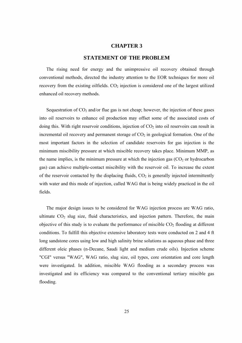
The rising need for energy and the unimpressive oil recovery obtained through
conventional methods, directed the industry attention to the EOR techniques for more oil
recovery from the existing oilfields. CO2 injection is considered one of the largest utilized
enhanced oil recovery methods.
Sequestration of CO2 and/or flue gas is not cheap; however, the injection of these gases
into oil reservoirs to enhance oil production may offset some of the associated costs of
doing this. With right reservoir conditions, injection of CO2 into oil reservoirs can result in
incremental oil recovery and permanent storage of CO2 in geological formation. One of the
most important factors in the selection of candidate reservoirs for gas injection is the
minimum miscibility pressure at which miscible recovery takes place. Minimum MMP, as
the name implies, is the minimum pressure at which the injection gas (CO2 or hydrocarbon
gas) can achieve multiple-contact miscibility with the reservoir oil. To increase the extent
of the reservoir contacted by the displacing fluids, CO2 is generally injected intermittently
with water and this mode of injection, called WAG that is being widely practiced in the oil
fields.
The major design issues to be considered for WAG injection process are WAG ratio,
ultimate CO2 slug size, fluid characteristics, and injection pattern. Therefore, the main
objective of this study is to evaluate the performance of miscible CO2 flooding at different
conditions. To fulfill this objective extensive laboratory tests were conducted on 2 and 4 ft
long sandstone cores using low and high salinity brine solutions as aqueous phase and three
different oleic phases (n-Decane, Saudi light and medium crude oils). Injection scheme
"CGI" versus "WAG", WAG ratio, slug size, oil types, core orientation and core length
were investigated. In addition, miscible WAG flooding as a secondary process was
investigated and its efficiency was compared to the conventional tertiary miscible gas
flooding.
26
CHAPTER 4
EXPERIMENTAL APPARATUS AND PROCEDURE
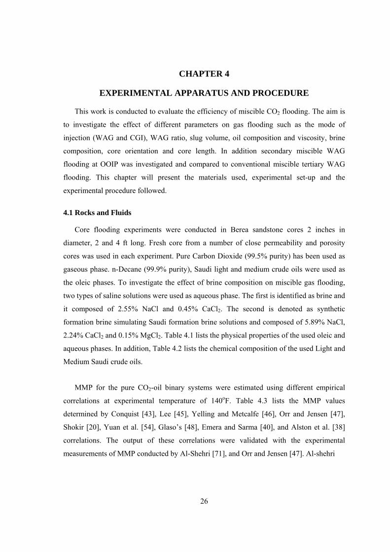
This work is conducted to evaluate the efficiency of miscible CO2 flooding. The aim is
to investigate the effect of different parameters on gas flooding such as the mode of
injection (WAG and CGI), WAG ratio, slug volume, oil composition and viscosity, brine
composition, core orientation and core length. In addition secondary miscible WAG
flooding at OOIP was investigated and compared to conventional miscible tertiary WAG
flooding. This chapter will present the materials used, experimental set-up and the
experimental procedure followed.
4.1 Rocks and Fluids
Core flooding experiments were conducted in Berea sandstone cores 2 inches in
diameter, 2 and 4 ft long. Fresh core from a number of close permeability and porosity
cores was used in each experiment. Pure Carbon Dioxide (99.5% purity) has been used as
gaseous phase. n-Decane (99.9% purity), Saudi light and medium crude oils were used as
the oleic phases. To investigate the effect of brine composition on miscible gas flooding,
two types of saline solutions were used as aqueous phase. The first is identified as brine and
it composed of 2.55% NaCl and 0.45% CaCl2. The second is denoted as synthetic
formation brine simulating Saudi formation brine solutions and composed of 5.89% NaCl,
2.24% CaCl2 and 0.15% MgCl2. Table 4.1 lists the physical properties of the used oleic and
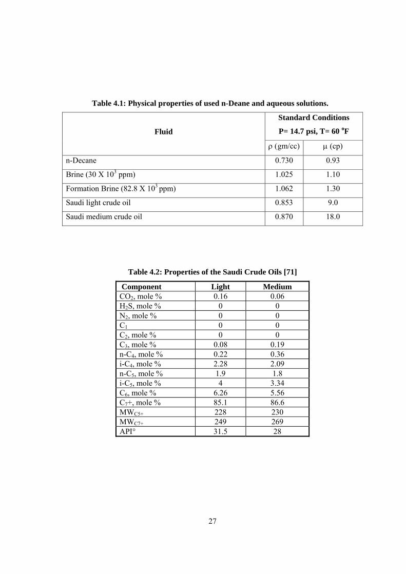
aqueous phases. In addition, Table 4.2 lists the chemical composition of the used Light and
Medium Saudi crude oils.
MMP for the pure CO2-oil binary systems were estimated using different empirical
correlations at experimental temperature of 140oF. Table 4.3 lists the MMP values
determined by Conquist [43], Lee [45], Yelling and Metcalfe [46], Orr and Jensen [47],
Shokir [20], Yuan et al. [54], Glaso’s [48], Emera and Sarma [40], and Alston et al. [38]
correlations. The output of these correlations were validated with the experimental
measurements of MMP conducted by Al-Shehri [71], and Orr and Jensen [47]. Al-shehri
27
Table 4.1: Physical properties of used n-Deane and aqueous solutions.
Standard Conditions
P= 14.7 psi, T= 60 oF Fluid
ρ (gm/cc) µ (cp)
n-Decane 0.730 0.93
Brine (30 X 103 ppm) 1.025 1.10
Formation Brine (82.8 X 10³ ppm) 1.062 1.30
Saudi light crude oil 0.853 9.0
Saudi medium crude oil 0.870 18.0
Table 4.2: Properties of the Saudi Crude Oils [71]
Component Light Medium CO2, mole % 0.16 0.06 H2S, mole % 0 0 N2, mole % 0 0 C1 0 0 C2, mole % 0 0 C3, mole % 0.08 0.19 n-C4, mole % 0.22 0.36 i-C4, mole % 2.28 2.09 n-C5, mole % 1.9 1.8 i-C5, mole % 4 3.34 C6, mole % 6.26 5.56 C7+, mole % 85.1 86.6 MWC5+ 228 230 MWC7+ 249 269 API° 31.5 28
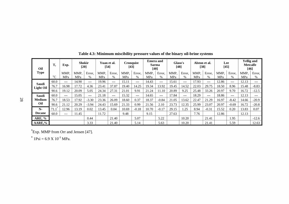
Table 4.3: Minimum miscibility pressure values of the binary oil-brine systems
T, Exp. Shokir [20]
Yuan et al. [54]
Cronquist [43]
Emera and Sarma
[40]
Glaso's [48]
Alston et al. [38]
Lee [45]
Yellig and Metcalfe
[46]
Oil Type
oC MMP, MPa
MMP, MPa
Error, %
MMP, MPa
Error, %
MMP, MPa
Error, %
MMP, MPa
Error, %
MMP, MPa
Error, %
MMP, MPa
Error, %
MMP, MPa
Error, %
MMP, MPa
Error, %
60.0 --- 14.90 --- 19.96 --- 15.11 --- 14.43 --- 15.61 --- 17.93 --- 12.86 --- 12.13 --- 76.7 16.98 17.72 4.36 23.41 37.87 19.40 14.25 19.34 13.92 19.45 14.52 22.03 29.75 18.50 8.96 15.48 -8.83
Saudi Light Oil
90.6 19.12 20.09 5.05 24.34 27.31 21.01 9.91 21.24 11.10 20.89 9.25 25.48 33.26 20.97 9.70 16.72 -12.5 60.0 --- 15.05 --- 21.18 --- 15.32 --- 14.65 --- 17.84 --- 18.29 --- 18.86 --- 12.13 --- 76.7 18.53 17.92 -3.30 23.36 26.09 18.60 0.37 18.37 -0.84 21.05 13.62 22.47 21.29 16.97 -8.42 14.66 -20.9
Saudi Medium
Oil 90.6 21.12 20.29 -3.94 24.43 15.69 21.33 0.99 21.56 2.10 23.73 12.35 25.99 23.07 20.97 -0.69 16.72 -20.8 71.1* 12.96 13.19 0.02 13.45 0.04 10.69 -0.18 10.70 -0.17 29.15 1.25 8.94 -0.31 15.52 0.20 13.83 0.07 N-
Decane 60.0 --- 11.45 11.72 9.48 9.15 27.63 7.76 12.86 12.13 ARE, % 0.44 21.40 5.07 5.22 10.20 21.41 1.95 -12.6 AARE,% 3.33 21.40 5.14 5.63 10.20 21.41 5.59 12.63
*Exp. MMP from Orr and Jensen [47]. * 1Psi = 6.9 X 10⁻³ MPa.
28
29
did his measurements on dead Saudi light and medium crud oils using slim tube at 76.7 and
90.6o C
To ensure good miscibility, the miscible floods were conducted at pressures slightly
higher than the MMP value determined by experimental measurements and all empirical
correlations mentioned above.
4.2 Experimental Setup
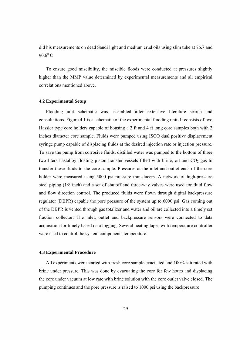
Flooding unit schematic was assembled after extensive literature search and
consultations. Figure 4.1 is a schematic of the experimental flooding unit. It consists of two
Hassler type core holders capable of housing a 2 ft and 4 ft long core samples both with 2
inches diameter core sample. Fluids were pumped using ISCO dual positive displacement
syringe pump capable of displacing fluids at the desired injection rate or injection pressure.
To save the pump from corrosive fluids, distilled water was pumped to the bottom of three
two liters hastalloy floating piston transfer vessels filled with brine, oil and CO2 gas to
transfer these fluids to the core sample. Pressures at the inlet and outlet ends of the core
holder were measured using 5000 psi pressure transducers. A network of high-pressure
steel piping (1/8 inch) and a set of shutoff and three-way valves were used for fluid flow
and flow direction control. The produced fluids were flown through digital backpressure
regulator (DBPR) capable the pore pressure of the system up to 6000 psi. Gas coming out
of the DBPR is vented through gas totalizer and water and oil are collected into a timely set
fraction collector. The inlet, outlet and backpressure sensors were connected to data
acquisition for timely based data logging. Several heating tapes with temperature controller
were used to control the system components temperature.
4.3 Experimental Procedure
All experiments were started with fresh core sample evacuated and 100% saturated with
brine under pressure. This was done by evacuating the core for few hours and displacing
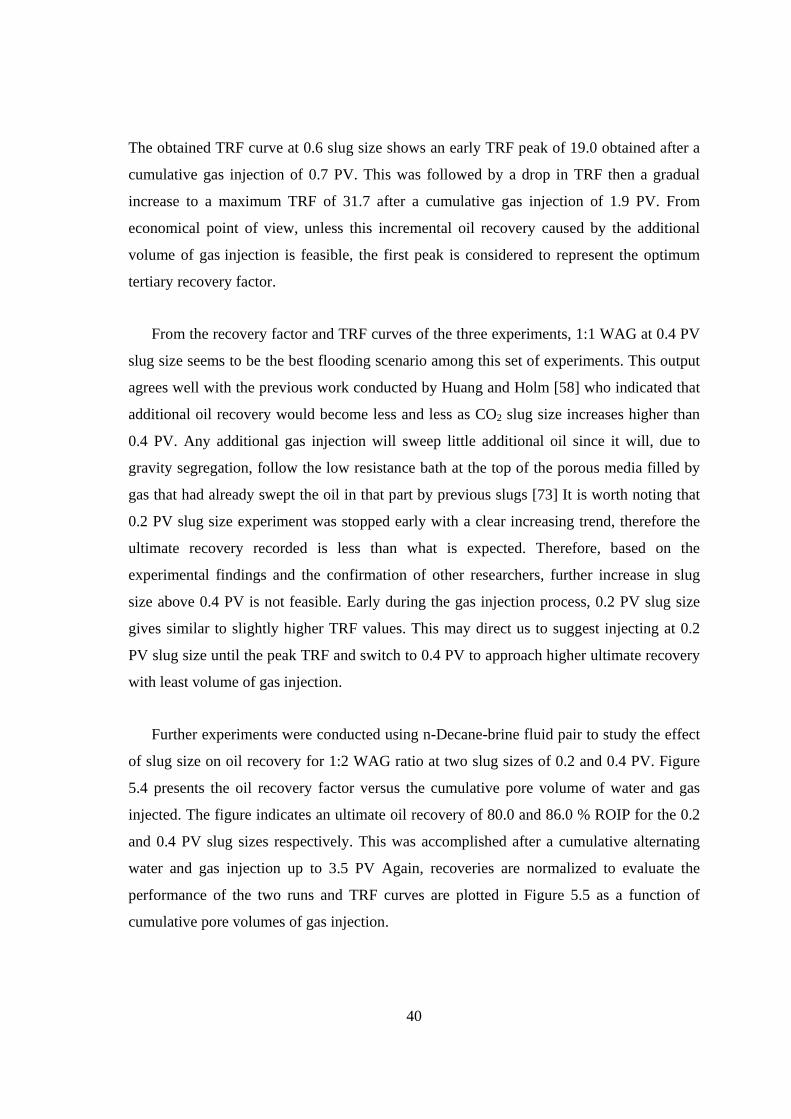
the core under vacuum at low rate with brine solution with the core outlet valve closed. The
pumping continues and the pore pressure is raised to 1000 psi using the backpressure
30
Figure 4.1: Schematic of the experimental set-up used in this study.
31
regulator. The pump is then shut down and the system was kept under pressure for a while.
The inlet valve was then closed and the outlet valve was open and the compressed
excessive brine is collected, weighed and subtracted with the lines dead volume from the
brine volume pumped to determine the pore volume and hence the porosity.
The system temperature and pressure was raised to 60οC and to a net effective pressure
(Pconfining – Ppore) of about 600 psi and permeability was determined by pumping the fully
saturated core at three different rates and measuring the pressure drop across the core ends.
Darcy law was then used to calculate the absolute permeability.
The core sample was restored to reservoir saturation by injecting oleic phase from the
oil transfer vessel into the brine-saturated core. This was done at 1.5 cc/min and continued
until water production ceases. Connate water saturation (Swi) was then determined using
material balance and end effective oil permeability (Ko) was measured using Darcy law.
The core is now at its initial water saturation, and the core is left for wettability restoration
and oil-water distributions refinement at the pore level. Water flooding was then started at
1.5 cc/min to residual oil saturation (Sor). The effluents volumes and pressure drop were
measured continuously and recorded as a function of time. This was continued until no
more oil is produced. Effective water permeability (Kw) was calculated using Darcy law
and post secondary water flooding residual oil saturation (Sor) was determined through
material balance.
At the end of the imbibition process (Berea is generally considered water-wet rock),
significant residual oil remains in the pore space. Therefore, tertiary CO2 flooding was
carried out subsequent to the secondary water flooding process. This was done in either
CGI or WAG injection schemes. The CGI was conducted by flooding the core with CO2 at
constant pressure. The injection pressure is chosen to be above the miscibility pressure of
the fluid pair used providing a flow rate range of 1.5-3 cc/min to ensure stability of the
flood. The brine and oil produced were collected in graduated glass tubes mounted in a
fraction collector while gas produced at the outlet end was vented through gas totalizer.

32
Water alternating gas injection is conducted by flooding CO2 and water alternately with
different WAG ratios at different slug sizes for every WAG ratio. Similar pressure in both
the brine and gas transfer vessels was maintained to prevent instabilities and early
breakthrough during the flood. Again, the brine and oil volumes produced were collected
in graduated glass tubes mounted in timely set fraction collector while gas produced was
vented through gas totalizer. The scaling rule of Leas and Rappaport [72] was used to
ensure stable oil, water and gas flooding.
33
CHAPTER 5
RESULTS AND DISCUSSIONS
Fifteen experiments were conducted to investigate the effect of different parameters on
oil recovery of miscible CO2 flooding. These parameters included the injection mode (CGI
and WAG), oil type, brine composition, WAG ratio, slug size, core orientation and core
length. WAG as a secondary process was investigated and compared to the conventional
tertiary WAG gas flooding. Table 5.1 lists the measured physical rock properties of
porosity and permeability, water flooding recovery factor, post secondary flooding end-
point saturations and end point effective permeability values for the experimental runs
conducted.
As mentioned previously, the core preparation consisted of different sequential steps,
including core saturation with aqueous phase, oil flooding to initial water saturation at the
flood out, and water flooding to residual oil saturation at flood out. The water flooding
process was applied to simulate the secondary oil recovery process. Subsequent to the
secondary flooding process, the core samples were subjected to miscible CO2 flooding to
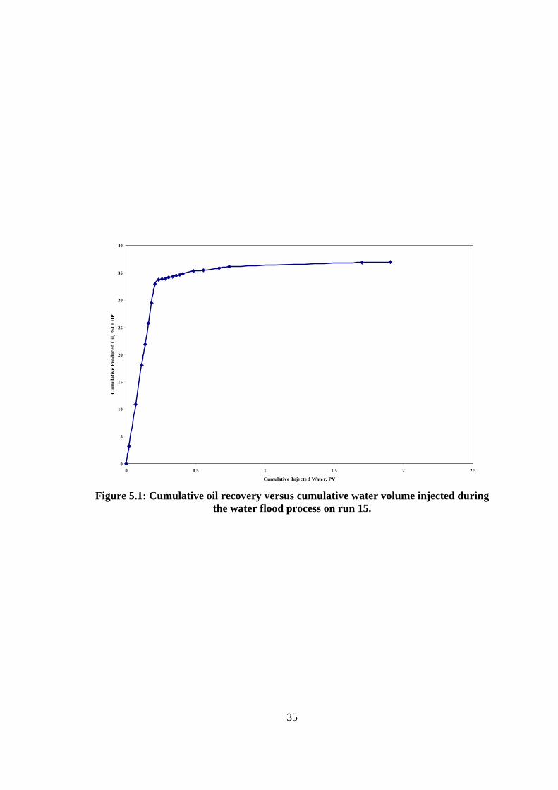
recover an incremental portion of the residual oil in place (ROIP). Figure 5.1 shows the
recovery curve of the water flooding process performed in run 15 listed in Table 5.1. This
curve is a typical representation of all the water flooding recovery curves obtained in all
conducted experiments. This chapter outlines the results for the miscible flooding
experimental work
Miscibility controls the microscopic displacement efficiency by affecting the capillary
number due to lowering of the interfacial tension. At the end of water flooding stage, the
core samples were miscibly flooded with CO2. Table 5.2 summarizes the experiments
conditions and the output of all conducted miscible gas flooding runs listing the oil
recovery (RF) as a percentage of residual oil in place (% ROIP), oil recovery as a
percentage of original oil in place (% OOIP), and the maximum tertiary recovery factor
(TRF) and the corresponding pore volume of gas injection. The obtained CO2 flooding
results and the effect of different investigated parameters are discussed extensively in the
following sections.
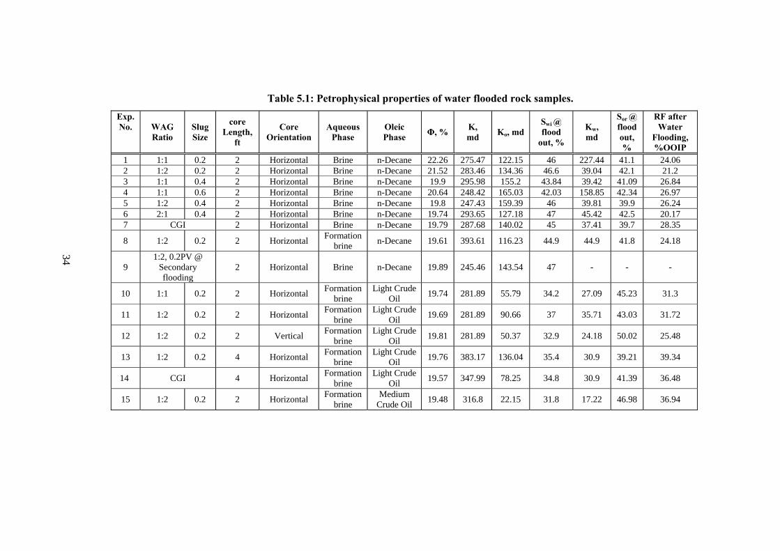
Table 5.1: Petrophysical properties of water flooded rock samples. Exp. No. WAG
Ratio Slug Size
core Length,
ft
Core Orientation
Aqueous Phase
Oleic Phase Φ, % K,
md Ko, md Swi @ flood
out, %
Kw, md
Sor @ flood out, %
RF after Water
Flooding, %OOIP
1 1:1 0.2 2 Horizontal Brine n-Decane 22.26 275.47 122.15 46 227.44 41.1 24.06 2 1:2 0.2 2 Horizontal Brine n-Decane 21.52 283.46 134.36 46.6 39.04 42.1 21.2 3 1:1 0.4 2 Horizontal Brine n-Decane 19.9 295.98 155.2 43.84 39.42 41.09 26.84 4 1:1 0.6 2 Horizontal Brine n-Decane 20.64 248.42 165.03 42.03 158.85 42.34 26.97 5 1:2 0.4 2 Horizontal Brine n-Decane 19.8 247.43 159.39 46 39.81 39.9 26.24 6 2:1 0.4 2 Horizontal Brine n-Decane 19.74 293.65 127.18 47 45.42 42.5 20.17 7 CGI 2 Horizontal Brine n-Decane 19.79 287.68 140.02 45 37.41 39.7 28.35
8 1:2 0.2 2 Horizontal Formation brine n-Decane 19.61 393.61 116.23 44.9 44.9 41.8 24.18
9 1:2, 0.2PV @
Secondary flooding
2 Horizontal Brine n-Decane 19.89 245.46 143.54 47 - - -
10 1:1 0.2 2 Horizontal Formation brine
Light Crude Oil 19.74 281.89 55.79 34.2 27.09 45.23 31.3
11 1:2 0.2 2 Horizontal Formation brine
Light Crude Oil 19.69 281.89 90.66 37 35.71 43.03 31.72
12 1:2 0.2 2 Vertical Formation brine
Light Crude Oil 19.81 281.89 50.37 32.9 24.18 50.02 25.48
13 1:2 0.2 4 Horizontal Formation brine
Light Crude Oil 19.76 383.17 136.04 35.4 30.9 39.21 39.34
14 CGI 4 Horizontal Formation brine
Light Crude Oil 19.57 347.99 78.25 34.8 30.9 41.39 36.48
15 1:2 0.2 2 Horizontal Formation brine
Medium Crude Oil 19.48 316.8 22.15 31.8 17.22 46.98 36.94
34
35
0
5
10
15
20
25
30
35
40
0 0.5 1 1.5 2 2.5
Cumulative Injected Water, PV
Cum
ulat
ive
Prod
uced
Oil,
%O
OIP
Figure 5.1: Cumulative oil recovery versus cumulative water volume injected during
the water flood process on run 15.
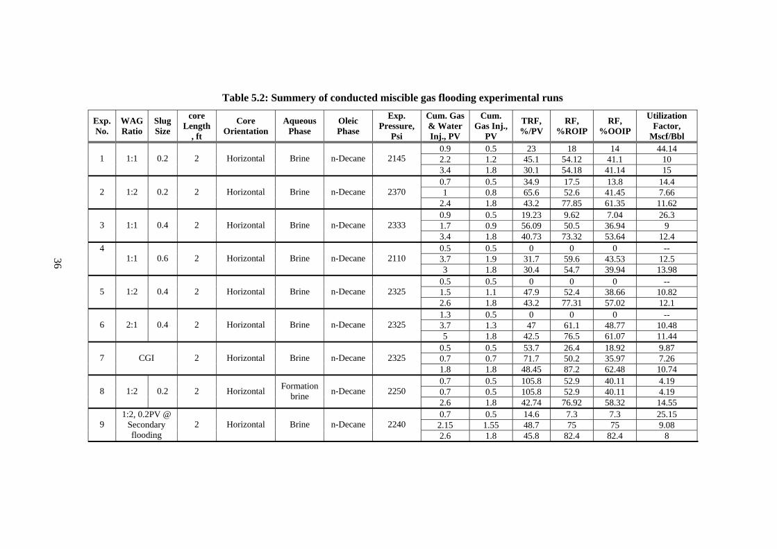
Table 5.2: Summery of conducted miscible gas flooding experimental runs
Exp. No.
WAG Ratio
Slug Size
core Length
, ft
Core Orientation
Aqueous Phase
Oleic Phase
Exp. Pressure,
Psi
Cum. Gas & Water Inj., PV
Cum. Gas Inj.,
PV
TRF, %/PV
RF, %ROIP
RF, %OOIP
Utilization Factor,
Mscf/Bbl 0.9 0.5 23 18 14 44.14 2.2 1.2 45.1 54.12 41.1 10 1 1:1 0.2 2 Horizontal Brine n-Decane 2145 3.4 1.8 30.1 54.18 41.14 15 0.7 0.5 34.9 17.5 13.8 14.4 1 0.8 65.6 52.6 41.45 7.66 2 1:2 0.2 2 Horizontal Brine n-Decane 2370
2.4 1.8 43.2 77.85 61.35 11.62 0.9 0.5 19.23 9.62 7.04 26.3 1.7 0.9 56.09 50.5 36.94 9 3 1:1 0.4 2 Horizontal Brine n-Decane 2333 3.4 1.8 40.73 73.32 53.64 12.4 0.5 0.5 0 0 0 -- 3.7 1.9 31.7 59.6 43.53 12.5
4 1:1 0.6 2 Horizontal Brine n-Decane 2110
3 1.8 30.4 54.7 39.94 13.98 0.5 0.5 0 0 0 -- 1.5 1.1 47.9 52.4 38.66 10.82 5 1:2 0.4 2 Horizontal Brine n-Decane 2325 2.6 1.8 43.2 77.31 57.02 12.1 1.3 0.5 0 0 0 -- 3.7 1.3 47 61.1 48.77 10.48 6 2:1 0.4 2 Horizontal Brine n-Decane 2325 5 1.8 42.5 76.5 61.07 11.44
0.5 0.5 53.7 26.4 18.92 9.87 0.7 0.7 71.7 50.2 35.97 7.26 7 CGI 2 Horizontal Brine n-Decane 2325 1.8 1.8 48.45 87.2 62.48 10.74 0.7 0.5 105.8 52.9 40.11 4.19 0.7 0.5 105.8 52.9 40.11 4.19 8 1:2 0.2 2 Horizontal Formation
brine n-Decane 2250 2.6 1.8 42.74 76.92 58.32 14.55 0.7 0.5 14.6 7.3 7.3 25.15
2.15 1.55 48.7 75 75 9.08 9 1:2, 0.2PV @
Secondary flooding
2 Horizontal Brine n-Decane 2240 2.6 1.8 45.8 82.4 82.4 8
36
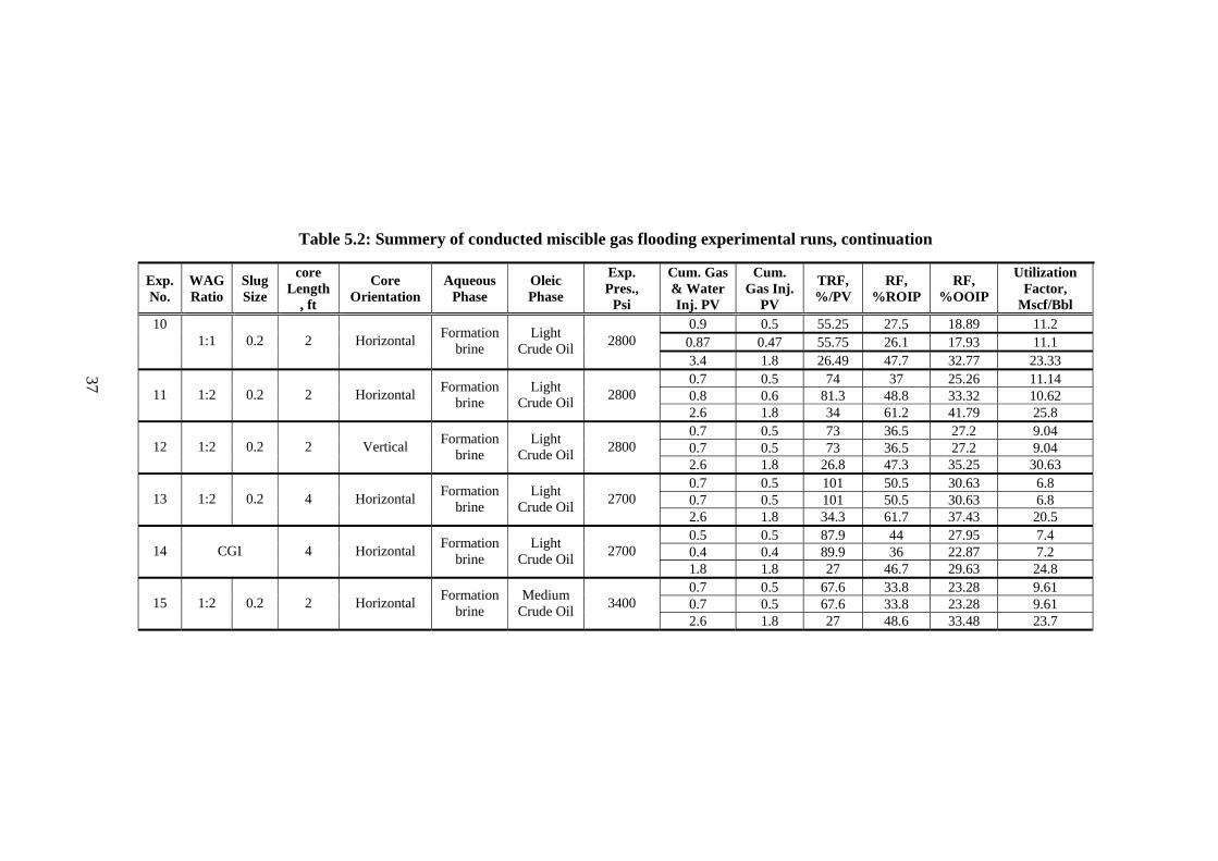
Table 5.2: Summery of conducted miscible gas flooding experimental runs, continuation
Exp. No.
WAG Ratio
Slug Size
core Length
, ft
Core Orientation
Aqueous Phase
Oleic Phase
Exp. Pres.,
Psi
Cum. Gas & Water Inj. PV
Cum. Gas Inj.
PV
TRF, %/PV
RF, %ROIP
RF, %OOIP
Utilization Factor,
Mscf/Bbl 0.9 0.5 55.25 27.5 18.89 11.2
0.87 0.47 55.75 26.1 17.93 11.1 10
1:1 0.2 2 Horizontal Formation brine
Light Crude Oil 2800
3.4 1.8 26.49 47.7 32.77 23.33 0.7 0.5 74 37 25.26 11.14 0.8 0.6 81.3 48.8 33.32 10.62 11 1:2 0.2 2 Horizontal Formation
brine Light
Crude Oil 2800 2.6 1.8 34 61.2 41.79 25.8 0.7 0.5 73 36.5 27.2 9.04 0.7 0.5 73 36.5 27.2 9.04 12 1:2 0.2 2 Vertical Formation
brine Light
Crude Oil 2800 2.6 1.8 26.8 47.3 35.25 30.63 0.7 0.5 101 50.5 30.63 6.8 0.7 0.5 101 50.5 30.63 6.8 13 1:2 0.2 4 Horizontal Formation
brine Light
Crude Oil 2700 2.6 1.8 34.3 61.7 37.43 20.5 0.5 0.5 87.9 44 27.95 7.4 0.4 0.4 89.9 36 22.87 7.2 14 CGI 4 Horizontal Formation
brine Light
Crude Oil 2700 1.8 1.8 27 46.7 29.63 24.8 0.7 0.5 67.6 33.8 23.28 9.61 0.7 0.5 67.6 33.8 23.28 9.61 15 1:2 0.2 2 Horizontal Formation
brine Medium
Crude Oil 3400 2.6 1.8 27 48.6 33.48 23.7
37
38
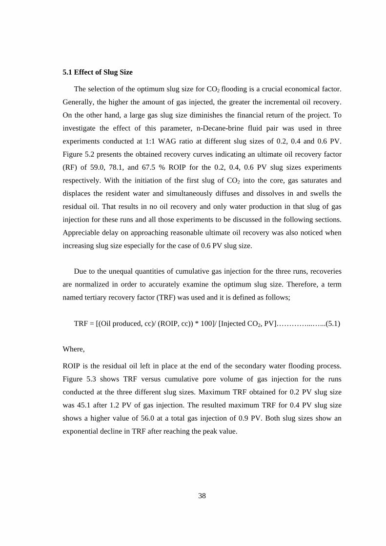
5.1 Effect of Slug Size
The selection of the optimum slug size for CO2 flooding is a crucial economical factor.
Generally, the higher the amount of gas injected, the greater the incremental oil recovery.
On the other hand, a large gas slug size diminishes the financial return of the project. To
investigate the effect of this parameter, n-Decane-brine fluid pair was used in three
experiments conducted at 1:1 WAG ratio at different slug sizes of 0.2, 0.4 and 0.6 PV.
Figure 5.2 presents the obtained recovery curves indicating an ultimate oil recovery factor
(RF) of 59.0, 78.1, and 67.5 % ROIP for the 0.2, 0.4, 0.6 PV slug sizes experiments
respectively. With the initiation of the first slug of CO2 into the core, gas saturates and
displaces the resident water and simultaneously diffuses and dissolves in and swells the
residual oil. That results in no oil recovery and only water production in that slug of gas
injection for these runs and all those experiments to be discussed in the following sections.
Appreciable delay on approaching reasonable ultimate oil recovery was also noticed when
increasing slug size especially for the case of 0.6 PV slug size.
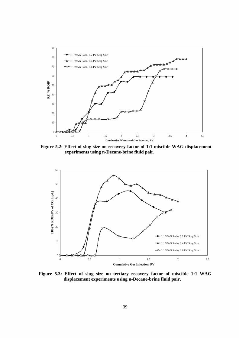
Due to the unequal quantities of cumulative gas injection for the three runs, recoveries
are normalized in order to accurately examine the optimum slug size. Therefore, a term
named tertiary recovery factor (TRF) was used and it is defined as follows;
TRF = [(Oil produced, cc)/ (ROIP, cc)) * 100]/ [Injected CO2, PV]…………...…...(5.1)
Where,
ROIP is the residual oil left in place at the end of the secondary water flooding process.
Figure 5.3 shows TRF versus cumulative pore volume of gas injection for the runs
conducted at the three different slug sizes. Maximum TRF obtained for 0.2 PV slug size
was 45.1 after 1.2 PV of gas injection. The resulted maximum TRF for 0.4 PV slug size
shows a higher value of 56.0 at a total gas injection of 0.9 PV. Both slug sizes show an
exponential decline in TRF after reaching the peak value.
39
0
10
20
30
40
50
60
70
80
90
0 0.5 1 1.5 2 2.5 3 3.5 4 4.5
Cumluative Water and Gas Injected, PV
RF,
% R
OIP
1:1 WAG Ratio, 0.2 PV Slug Size
1:1 WAG Ratio, 0.4 PV Slug Size
1:1 WAG Ratio, 0.6 PV Slug Size
Figure 5.2: Effect of slug size on recovery factor of 1:1 miscible WAG displacement
experiments using n-Decane-brine fluid pair.
0
10
20
30
40
50
60
0 0.5 1 1.5 2 2.5
Cumulative Gas Injection, PV
TR
F(%
RO
IP/P
V o
f CO
2 Inj
d.)
1:1 WAG Ratio, 0.2 PV Slug Size
1:1 WAG Ratio, 0.4 PV Slug Size
1:1 WAG Ratio, 0.6 PV Slug Size
Figure 5.3: Effect of slug size on tertiary recovery factor of miscible 1:1 WAG
displacement experiments using n-Decane-brine fluid pair.
40
The obtained TRF curve at 0.6 slug size shows an early TRF peak of 19.0 obtained after a
cumulative gas injection of 0.7 PV. This was followed by a drop in TRF then a gradual
increase to a maximum TRF of 31.7 after a cumulative gas injection of 1.9 PV. From
economical point of view, unless this incremental oil recovery caused by the additional
volume of gas injection is feasible, the first peak is considered to represent the optimum
tertiary recovery factor.
From the recovery factor and TRF curves of the three experiments, 1:1 WAG at 0.4 PV
slug size seems to be the best flooding scenario among this set of experiments. This output
agrees well with the previous work conducted by Huang and Holm [58] who indicated that
additional oil recovery would become less and less as CO2 slug size increases higher than
0.4 PV. Any additional gas injection will sweep little additional oil since it will, due to
gravity segregation, follow the low resistance bath at the top of the porous media filled by
gas that had already swept the oil in that part by previous slugs [73] It is worth noting that
0.2 PV slug size experiment was stopped early with a clear increasing trend, therefore the
ultimate recovery recorded is less than what is expected. Therefore, based on the
experimental findings and the confirmation of other researchers, further increase in slug
size above 0.4 PV is not feasible. Early during the gas injection process, 0.2 PV slug size
gives similar to slightly higher TRF values. This may direct us to suggest injecting at 0.2
PV slug size until the peak TRF and switch to 0.4 PV to approach higher ultimate recovery
with least volume of gas injection.
Further experiments were conducted using n-Decane-brine fluid pair to study the effect
of slug size on oil recovery for 1:2 WAG ratio at two slug sizes of 0.2 and 0.4 PV. Figure
5.4 presents the oil recovery factor versus the cumulative pore volume of water and gas
injected. The figure indicates an ultimate oil recovery of 80.0 and 86.0 % ROIP for the 0.2
and 0.4 PV slug sizes respectively. This was accomplished after a cumulative alternating
water and gas injection up to 3.5 PV Again, recoveries are normalized to evaluate the
performance of the two runs and TRF curves are plotted in Figure 5.5 as a function of
cumulative pore volumes of gas injection.
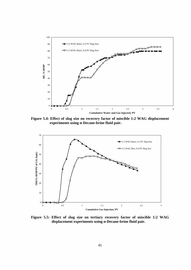
41
0
10
20
30
40
50
60
70
80
90
100
0 0.5 1 1.5 2 2.5 3 3.5 4
Cumulative Water and Gas Injected, PV
RF,
% R
OIP
1:2 WAG Ratio, 0.2 PV Slug Size
1:2 WAG Ratio, 0.4 PV Slug Size
Figure 5.4: Effect of slug size on recovery factor of miscible 1:2 WAG displacement
experiments using n-Decane-brine fluid pair.
0
10
20
30
40
50
60
70
0 0.5 1 1.5 2 2.5 3
Cumulative Gas Injection, PV
TR
F(%
RO
IP/P
V o
f CO
2 Inj
d.)
1:2 WAG Ratio, 0.2 PV Slug Size
1:2 WAG Rtio, 0.4 PV Slug Size
Figure 5.5: Effect of slug size on tertiary recovery factor of miscible 1:2 WAG
displacement experiments using n-Decane-brine fluid pair.
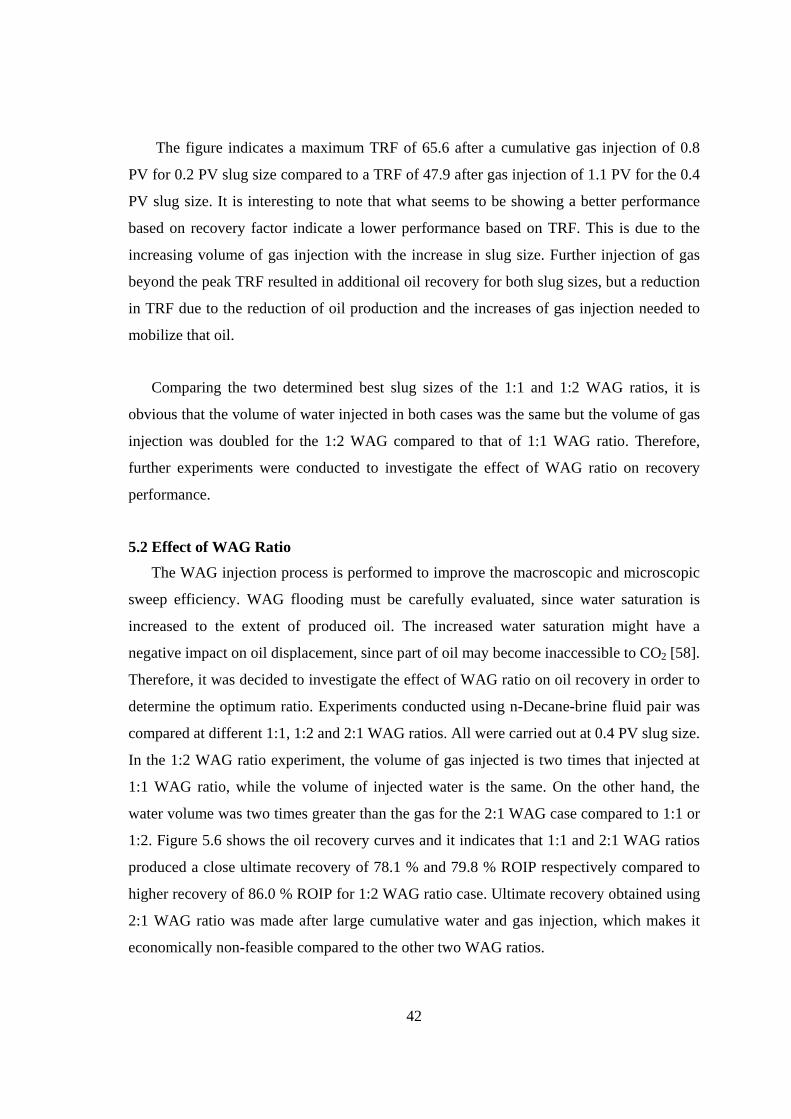
42
The figure indicates a maximum TRF of 65.6 after a cumulative gas injection of 0.8
PV for 0.2 PV slug size compared to a TRF of 47.9 after gas injection of 1.1 PV for the 0.4
PV slug size. It is interesting to note that what seems to be showing a better performance
based on recovery factor indicate a lower performance based on TRF. This is due to the
increasing volume of gas injection with the increase in slug size. Further injection of gas
beyond the peak TRF resulted in additional oil recovery for both slug sizes, but a reduction
in TRF due to the reduction of oil production and the increases of gas injection needed to
mobilize that oil.
Comparing the two determined best slug sizes of the 1:1 and 1:2 WAG ratios, it is
obvious that the volume of water injected in both cases was the same but the volume of gas
injection was doubled for the 1:2 WAG compared to that of 1:1 WAG ratio. Therefore,
further experiments were conducted to investigate the effect of WAG ratio on recovery
performance.
5.2 Effect of WAG Ratio
The WAG injection process is performed to improve the macroscopic and microscopic
sweep efficiency. WAG flooding must be carefully evaluated, since water saturation is
increased to the extent of produced oil. The increased water saturation might have a
negative impact on oil displacement, since part of oil may become inaccessible to CO2 [58].
Therefore, it was decided to investigate the effect of WAG ratio on oil recovery in order to
determine the optimum ratio. Experiments conducted using n-Decane-brine fluid pair was
compared at different 1:1, 1:2 and 2:1 WAG ratios. All were carried out at 0.4 PV slug size.
In the 1:2 WAG ratio experiment, the volume of gas injected is two times that injected at
1:1 WAG ratio, while the volume of injected water is the same. On the other hand, the
water volume was two times greater than the gas for the 2:1 WAG case compared to 1:1 or
1:2. Figure 5.6 shows the oil recovery curves and it indicates that 1:1 and 2:1 WAG ratios
produced a close ultimate recovery of 78.1 % and 79.8 % ROIP respectively compared to
higher recovery of 86.0 % ROIP for 1:2 WAG ratio case. Ultimate recovery obtained using
2:1 WAG ratio was made after large cumulative water and gas injection, which makes it
economically non-feasible compared to the other two WAG ratios.
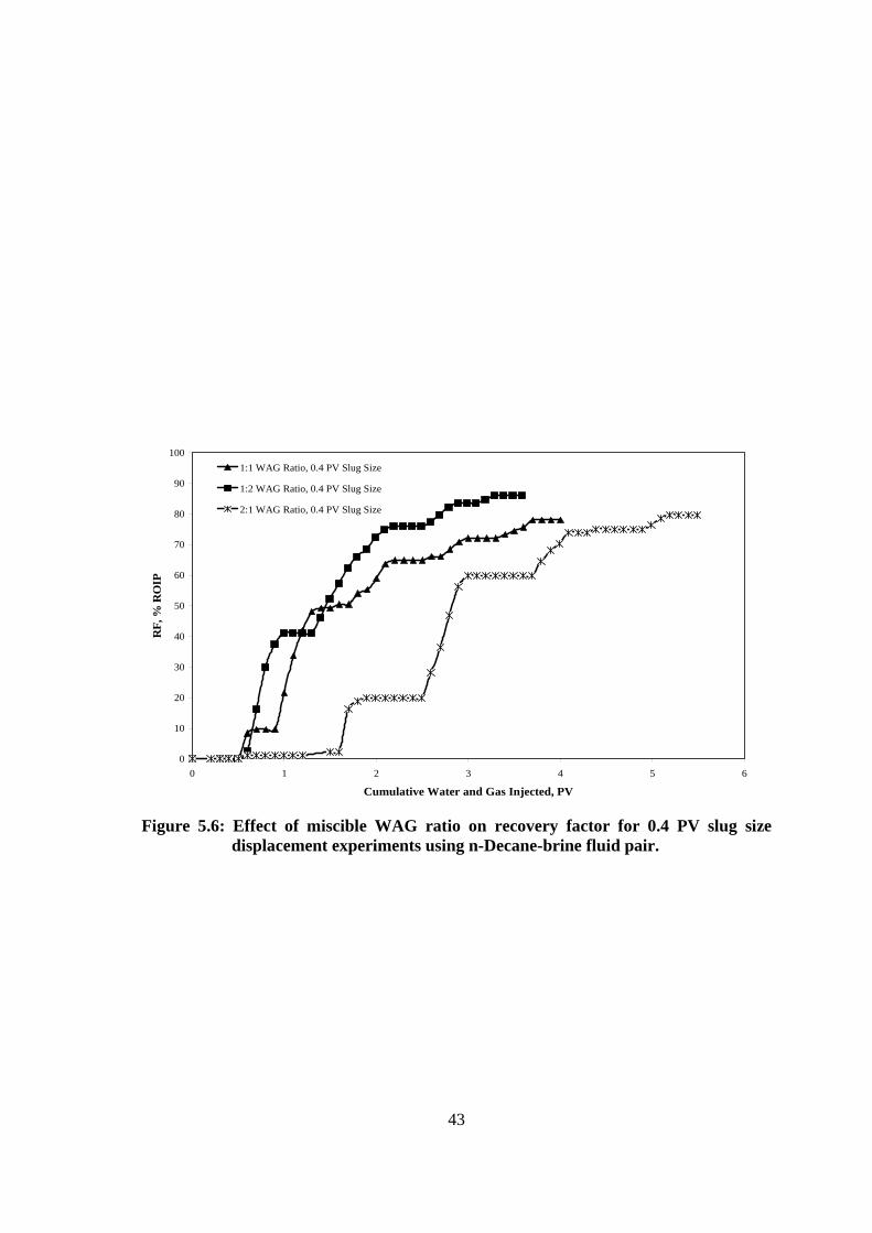
43
0
10
20
30
40
50
60
70
80
90
100
0 1 2 3 4 5 6
Cumulative Water and Gas Injected, PV
RF,
% R
OIP
1:1 WAG Ratio, 0.4 PV Slug Size
1:2 WAG Ratio, 0.4 PV Slug Size
2:1 WAG Ratio, 0.4 PV Slug Size
Figure 5.6: Effect of miscible WAG ratio on recovery factor for 0.4 PV slug size
displacement experiments using n-Decane-brine fluid pair.
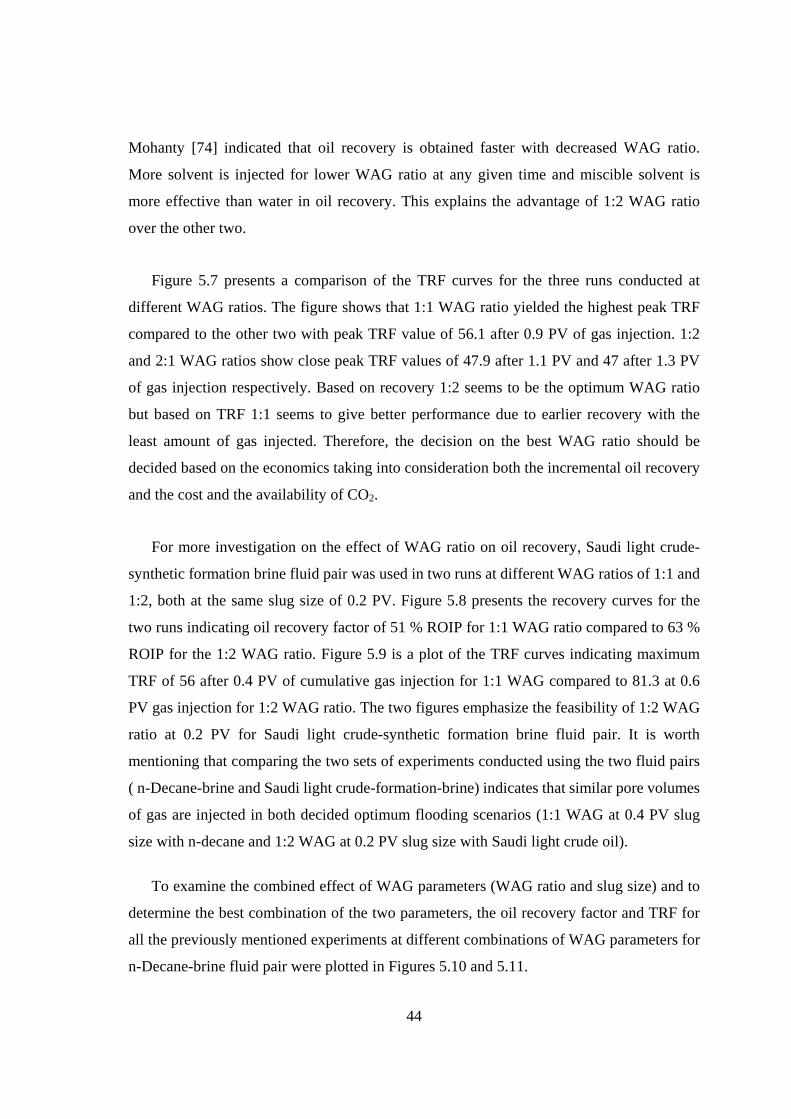
44
Mohanty [74] indicated that oil recovery is obtained faster with decreased WAG ratio.
More solvent is injected for lower WAG ratio at any given time and miscible solvent is
more effective than water in oil recovery. This explains the advantage of 1:2 WAG ratio
over the other two.
Figure 5.7 presents a comparison of the TRF curves for the three runs conducted at
different WAG ratios. The figure shows that 1:1 WAG ratio yielded the highest peak TRF
compared to the other two with peak TRF value of 56.1 after 0.9 PV of gas injection. 1:2
and 2:1 WAG ratios show close peak TRF values of 47.9 after 1.1 PV and 47 after 1.3 PV
of gas injection respectively. Based on recovery 1:2 seems to be the optimum WAG ratio
but based on TRF 1:1 seems to give better performance due to earlier recovery with the
least amount of gas injected. Therefore, the decision on the best WAG ratio should be
decided based on the economics taking into consideration both the incremental oil recovery
and the cost and the availability of CO2.
For more investigation on the effect of WAG ratio on oil recovery, Saudi light crude-
synthetic formation brine fluid pair was used in two runs at different WAG ratios of 1:1 and
1:2, both at the same slug size of 0.2 PV. Figure 5.8 presents the recovery curves for the
two runs indicating oil recovery factor of 51 % ROIP for 1:1 WAG ratio compared to 63 %
ROIP for the 1:2 WAG ratio. Figure 5.9 is a plot of the TRF curves indicating maximum
TRF of 56 after 0.4 PV of cumulative gas injection for 1:1 WAG compared to 81.3 at 0.6
PV gas injection for 1:2 WAG ratio. The two figures emphasize the feasibility of 1:2 WAG
ratio at 0.2 PV for Saudi light crude-synthetic formation brine fluid pair. It is worth
mentioning that comparing the two sets of experiments conducted using the two fluid pairs
( n-Decane-brine and Saudi light crude-formation-brine) indicates that similar pore volumes
of gas are injected in both decided optimum flooding scenarios (1:1 WAG at 0.4 PV slug
size with n-decane and 1:2 WAG at 0.2 PV slug size with Saudi light crude oil).
To examine the combined effect of WAG parameters (WAG ratio and slug size) and to
determine the best combination of the two parameters, the oil recovery factor and TRF for
all the previously mentioned experiments at different combinations of WAG parameters for
n-Decane-brine fluid pair were plotted in Figures 5.10 and 5.11.
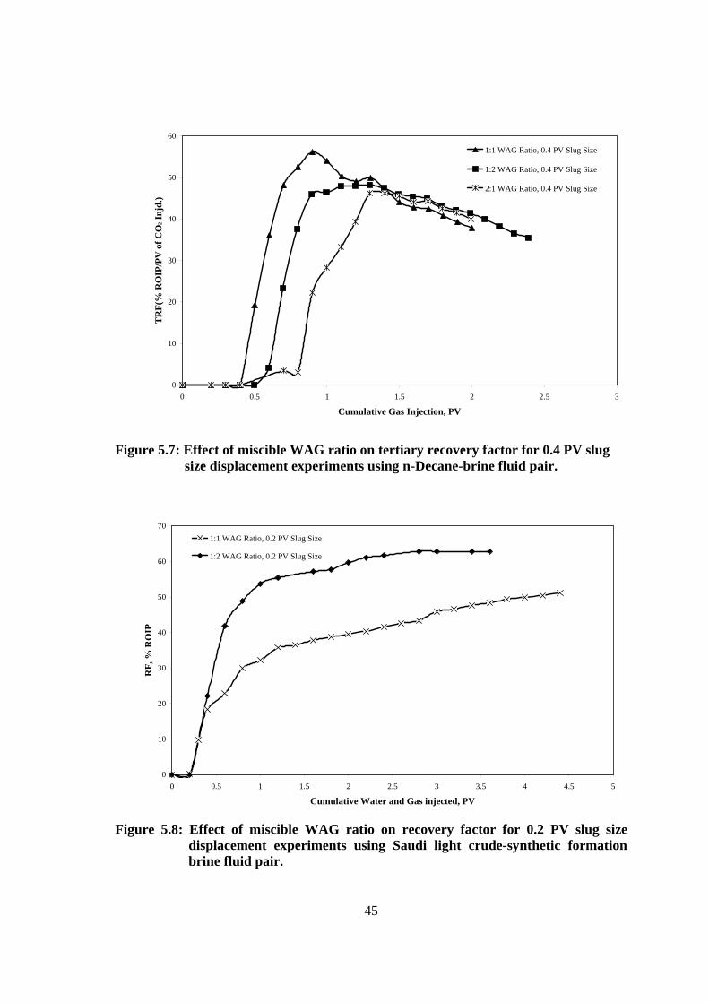
45
0
10
20
30
40
50
60
0 0.5 1 1.5 2 2.5 3
Cumulative Gas Injection, PV
TR
F(%
RO
IP/P
V o
f CO
2 Inj
d.)
1:1 WAG Ratio, 0.4 PV Slug Size
1:2 WAG Ratio, 0.4 PV Slug Size
2:1 WAG Ratio, 0.4 PV Slug Size
Figure 5.7: Effect of miscible WAG ratio on tertiary recovery factor for 0.4 PV slug size displacement experiments using n-Decane-brine fluid pair.
0
10
20
30
40
50
60
70
0 0.5 1 1.5 2 2.5 3 3.5 4 4.5 5
Cumulative Water and Gas injected, PV
RF,
% R
OIP
1:1 WAG Ratio, 0.2 PV Slug Size
1:2 WAG Ratio, 0.2 PV Slug Size
Figure 5.8: Effect of miscible WAG ratio on recovery factor for 0.2 PV slug size
displacement experiments using Saudi light crude-synthetic formation brine fluid pair.
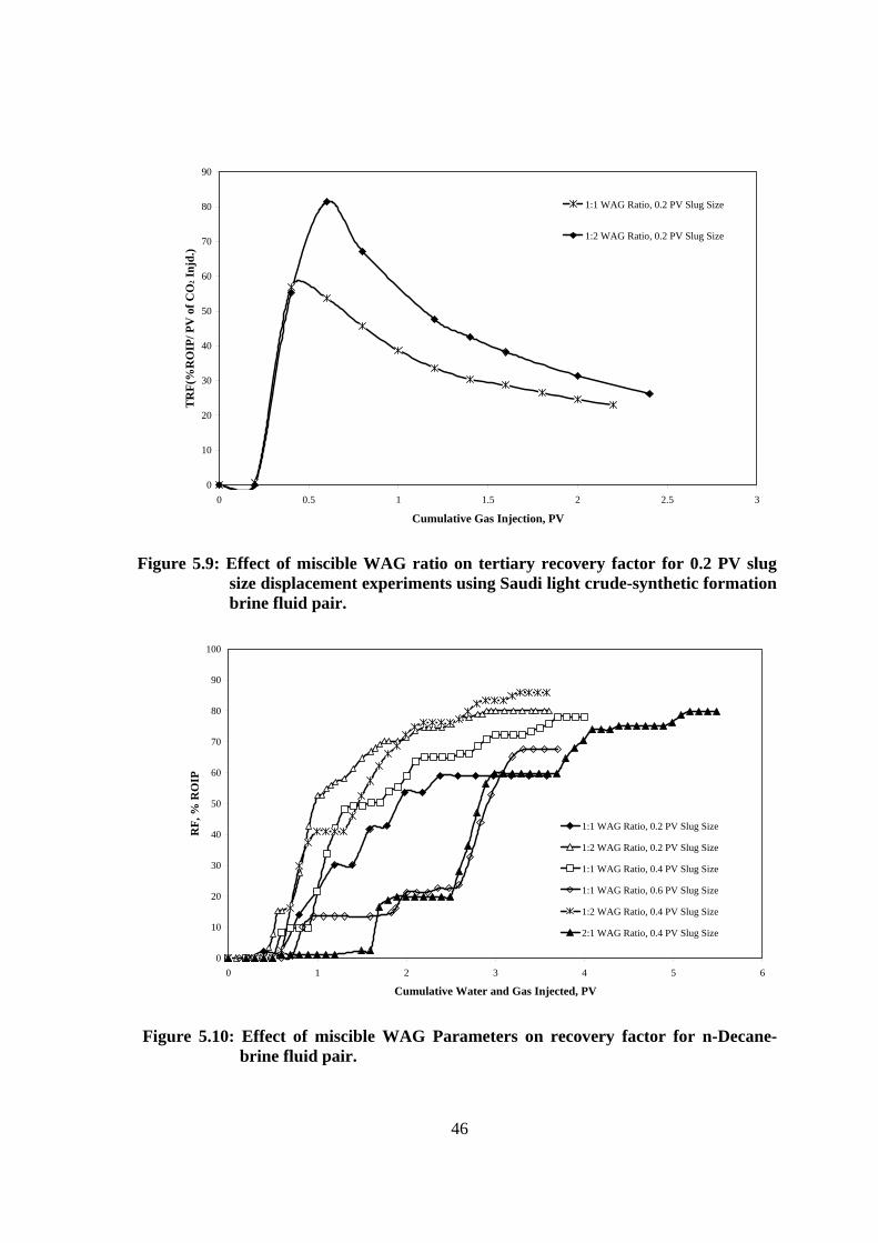
46
0
10
20
30
40
50
60
70
80
90
0 0.5 1 1.5 2 2.5 3
Cumulative Gas Injection, PV
TR
F(%
RO
IP/ P
V o
f CO
2 Inj
d.)
1:1 WAG Ratio, 0.2 PV Slug Size
1:2 WAG Ratio, 0.2 PV Slug Size
Figure 5.9: Effect of miscible WAG ratio on tertiary recovery factor for 0.2 PV slug size displacement experiments using Saudi light crude-synthetic formation brine fluid pair.
0
10
20
30
40
50
60
70
80
90
100
0 1 2 3 4 5 6
Cumulative Water and Gas Injected, PV
RF,
% R
OIP
1:1 WAG Ratio, 0.2 PV Slug Size
1:2 WAG Ratio, 0.2 PV Slug Size
1:1 WAG Ratio, 0.4 PV Slug Size
1:1 WAG Ratio, 0.6 PV Slug Size
1:2 WAG Ratio, 0.4 PV Slug Size
2:1 WAG Ratio, 0.4 PV Slug Size
Figure 5.10: Effect of miscible WAG Parameters on recovery factor for n-Decane-brine fluid pair.
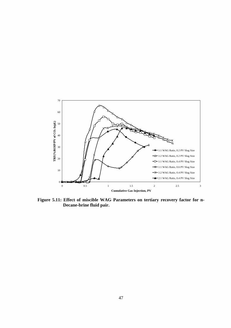
47
0
10
20
30
40
50
60
70
0 0.5 1 1.5 2 2.5 3
Cumulative Gas Injection, PV
TR
F(%
RO
IP/P
V o
f CO
2 Inj
d.)
1:1 WAG Ratio, 0.2 PV Slug Size
1:2 WAG Ratio, 0.2 PV Slug Size
1:1 WAG Ratio, 0.4 PV Slug Size
1:1 WAG Ratio, 0.6 PV Slug Size
1:2 WAG Ratio, 0.4 PV Slug Size
2:1 WAG Ratio, 0.4 PV Slug Size
Figure 5.11: Effect of miscible WAG Parameters on tertiary recovery factor for n-
Decane-brine fluid pair.
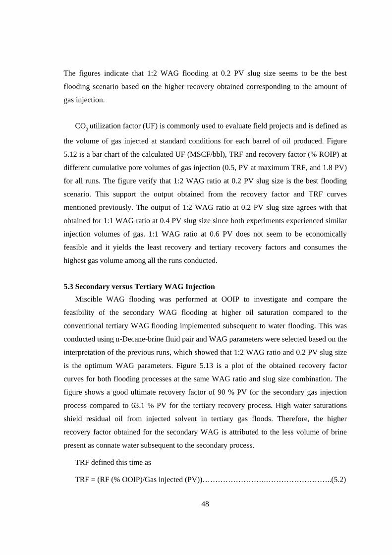
48
The figures indicate that 1:2 WAG flooding at 0.2 PV slug size seems to be the best
flooding scenario based on the higher recovery obtained corresponding to the amount of
gas injection.
CO2 utilization factor (UF) is commonly used to evaluate field projects and is defined as
the volume of gas injected at standard conditions for each barrel of oil produced. Figure
5.12 is a bar chart of the calculated UF (MSCF/bbl), TRF and recovery factor (% ROIP) at
different cumulative pore volumes of gas injection (0.5, PV at maximum TRF, and 1.8 PV)
for all runs. The figure verify that 1:2 WAG ratio at 0.2 PV slug size is the best flooding
scenario. This support the output obtained from the recovery factor and TRF curves
mentioned previously. The output of 1:2 WAG ratio at 0.2 PV slug size agrees with that
obtained for 1:1 WAG ratio at 0.4 PV slug size since both experiments experienced similar
injection volumes of gas. 1:1 WAG ratio at 0.6 PV does not seem to be economically
feasible and it yields the least recovery and tertiary recovery factors and consumes the
highest gas volume among all the runs conducted.
5.3 Secondary versus Tertiary WAG Injection
Miscible WAG flooding was performed at OOIP to investigate and compare the
feasibility of the secondary WAG flooding at higher oil saturation compared to the
conventional tertiary WAG flooding implemented subsequent to water flooding. This was
conducted using n-Decane-brine fluid pair and WAG parameters were selected based on the
interpretation of the previous runs, which showed that 1:2 WAG ratio and 0.2 PV slug size
is the optimum WAG parameters. Figure 5.13 is a plot of the obtained recovery factor
curves for both flooding processes at the same WAG ratio and slug size combination. The
figure shows a good ultimate recovery factor of 90 % PV for the secondary gas injection
process compared to 63.1 % PV for the tertiary recovery process. High water saturations
shield residual oil from injected solvent in tertiary gas floods. Therefore, the higher
recovery factor obtained for the secondary WAG is attributed to the less volume of brine
present as connate water subsequent to the secondary process.
TRF defined this time as
TRF = (RF (% OOIP)/Gas injected (PV))…………………….……………………..(5.2)
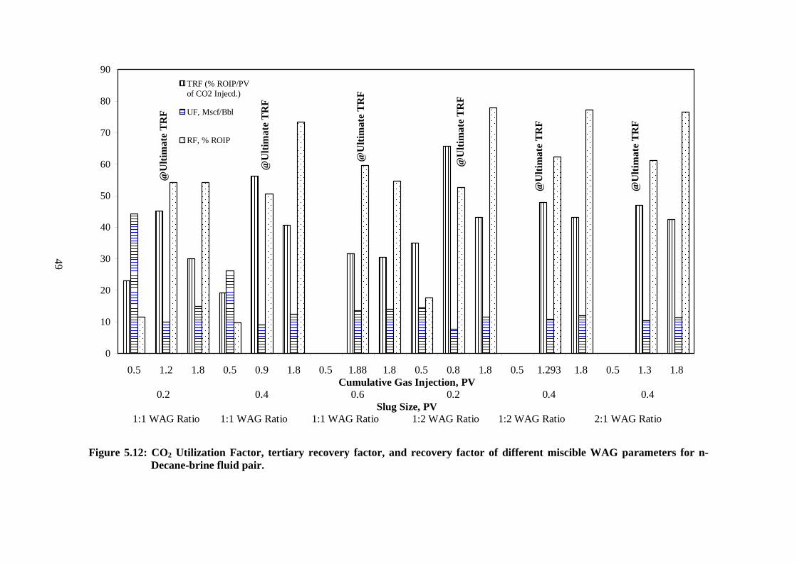
0
10
20
30
40
50
60
70
80
90TRF (% ROIP/PVof CO2 Injecd.)
UF, Mscf/Bbl
RF, % ROIP
@U
ltim
ate
TR
F
@U
ltim
ate
TR
F
@U
ltim
ate
TR
F
@U
ltim
ate
TR
F
@U
ltim
ate
TR
F
@U
ltim
ate
TR
F
0.5 1.2 1.8 0.5 0.9 1.8 0.5 1.88 1.8 0.5 0.8 1.8 0.5 1.293 1.8 0.5 1.3 1.8 Cumulative Gas Injection, PV
0.2 0.4 0.6 0.2 0.4 0.4 Slug Size, PV
1:1 WAG Ratio 1:1 WAG Ratio 1:1 WAG Ratio 1:2 WAG Ratio 1:2 WAG Ratio 2:1 WAG Ratio
Figure 5.12: CO2 Utilization Factor, tertiary recovery factor, and recovery factor of different miscible WAG parameters for n-Decane-brine fluid pair.
49
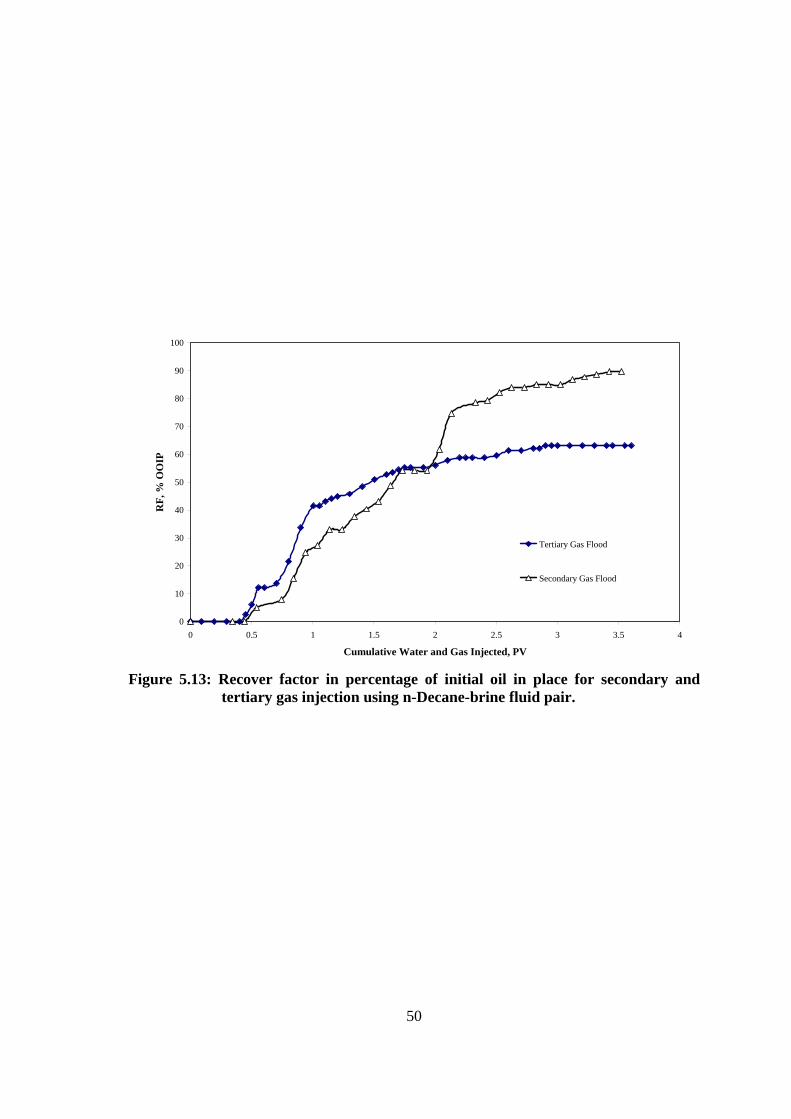
50
0
10
20
30
40
50
60
70
80
90
100
0 0.5 1 1.5 2 2.5 3 3.5 4
Cumulative Water and Gas Injected, PV
RF,
% O
OIP
Tertiary Gas Flood
Secondary Gas Flood
Figure 5.13: Recover factor in percentage of initial oil in place for secondary and
tertiary gas injection using n-Decane-brine fluid pair.
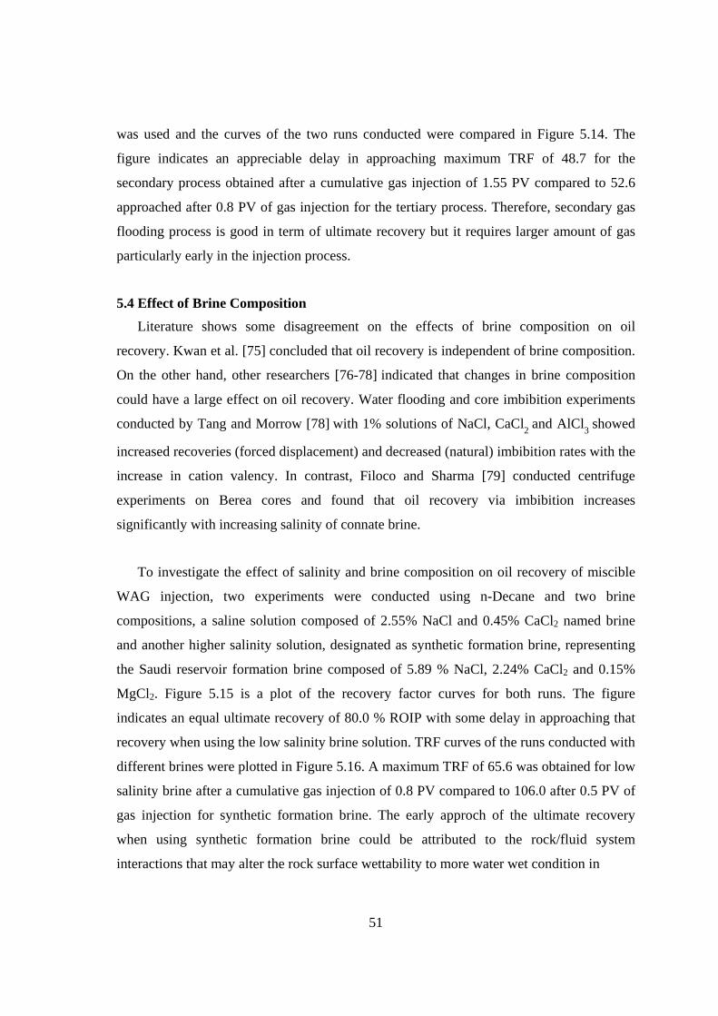
51
was used and the curves of the two runs conducted were compared in Figure 5.14. The
figure indicates an appreciable delay in approaching maximum TRF of 48.7 for the
secondary process obtained after a cumulative gas injection of 1.55 PV compared to 52.6
approached after 0.8 PV of gas injection for the tertiary process. Therefore, secondary gas
flooding process is good in term of ultimate recovery but it requires larger amount of gas
particularly early in the injection process.
5.4 Effect of Brine Composition
Literature shows some disagreement on the effects of brine composition on oil
recovery. Kwan et al. [75] concluded that oil recovery is independent of brine composition.
On the other hand, other researchers [76-78] indicated that changes in brine composition
could have a large effect on oil recovery. Water flooding and core imbibition experiments
conducted by Tang and Morrow [78] with 1% solutions of NaCl, CaCl2 and AlCl3 showed
increased recoveries (forced displacement) and decreased (natural) imbibition rates with the
increase in cation valency. In contrast, Filoco and Sharma [79] conducted centrifuge
experiments on Berea cores and found that oil recovery via imbibition increases
significantly with increasing salinity of connate brine.
To investigate the effect of salinity and brine composition on oil recovery of miscible
WAG injection, two experiments were conducted using n-Decane and two brine
compositions, a saline solution composed of 2.55% NaCl and 0.45% CaCl2 named brine
and another higher salinity solution, designated as synthetic formation brine, representing
the Saudi reservoir formation brine composed of 5.89 % NaCl, 2.24% CaCl2 and 0.15%
MgCl2. Figure 5.15 is a plot of the recovery factor curves for both runs. The figure
indicates an equal ultimate recovery of 80.0 % ROIP with some delay in approaching that
recovery when using the low salinity brine solution. TRF curves of the runs conducted with
different brines were plotted in Figure 5.16. A maximum TRF of 65.6 was obtained for low
salinity brine after a cumulative gas injection of 0.8 PV compared to 106.0 after 0.5 PV of
gas injection for synthetic formation brine. The early approch of the ultimate recovery
when using synthetic formation brine could be attributed to the rock/fluid system
interactions that may alter the rock surface wettability to more water wet condition in
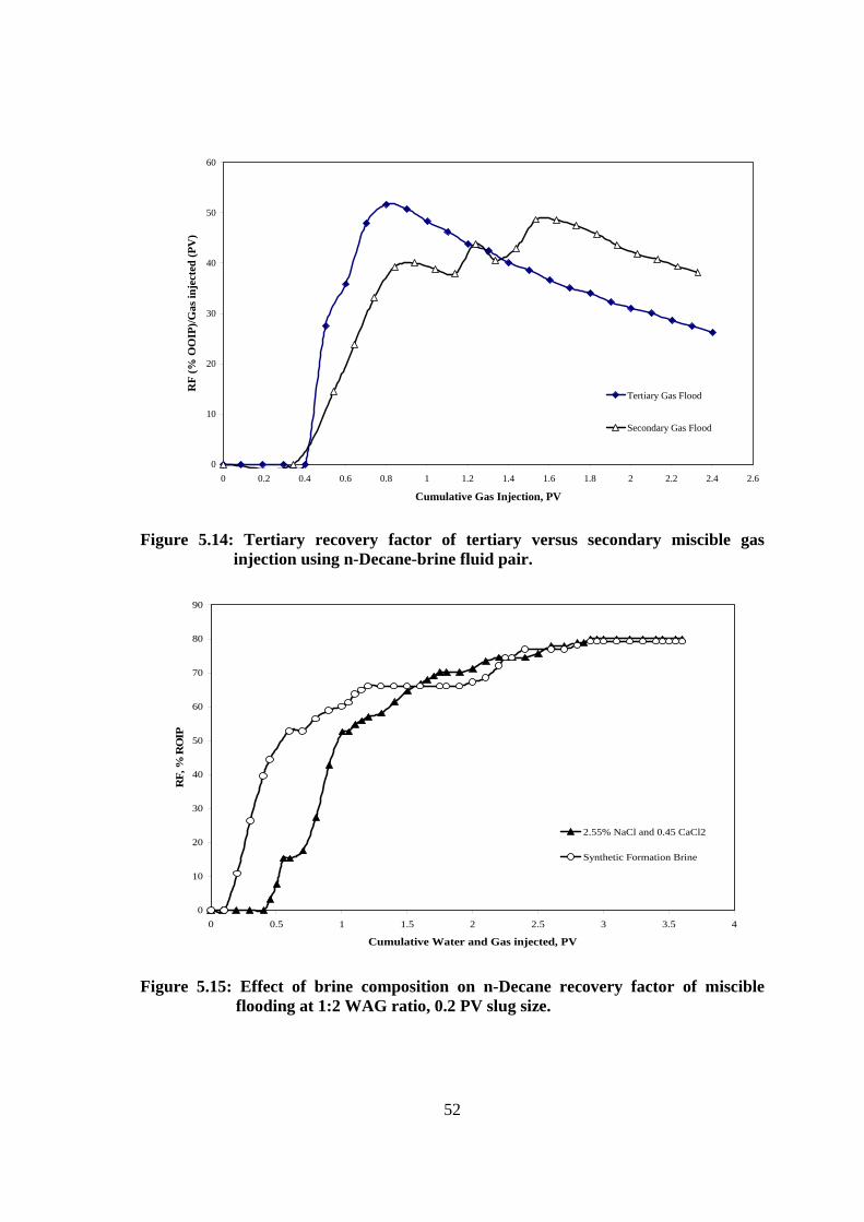
52
0
10
20
30
40
50
60
0 0.2 0.4 0.6 0.8 1 1.2 1.4 1.6 1.8 2 2.2 2.4 2.6
Cumulative Gas Injection, PV
RF
(% O
OIP
)/Gas
inje
cted
(PV
)
Tertiary Gas Flood
Secondary Gas Flood
Figure 5.14: Tertiary recovery factor of tertiary versus secondary miscible gas
injection using n-Decane-brine fluid pair.
0
10
20
30
40
50
60
70
80
90
0 0.5 1 1.5 2 2.5 3 3.5 4
Cumulative Water and Gas injected, PV
RF,
% R
OIP
2.55% NaCl and 0.45 CaCl2
Synthetic Formation Brine
Figure 5.15: Effect of brine composition on n-Decane recovery factor of miscible
flooding at 1:2 WAG ratio, 0.2 PV slug size.
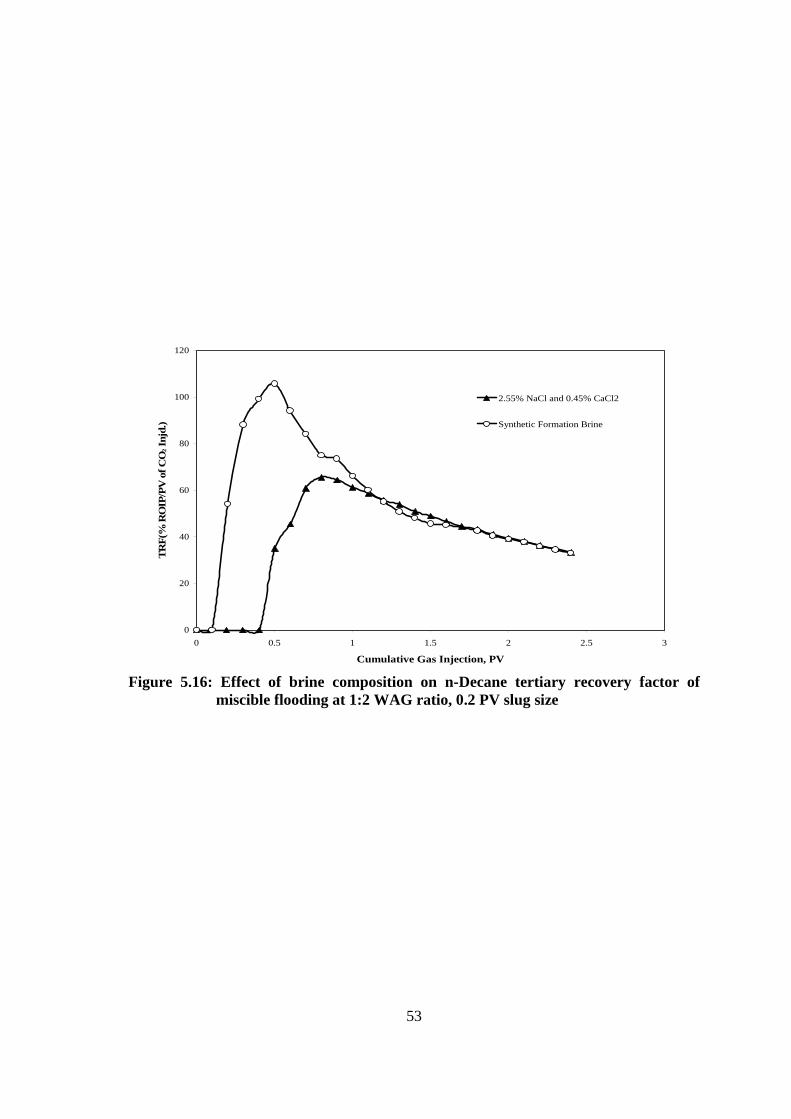
53
0
20
40
60
80
100
120
0 0.5 1 1.5 2 2.5 3
Cumulative Gas Injection, PV
TR
F(%
RO
IP/P
V o
f CO
2 Inj
d.)
2.55% NaCl and 0.45% CaCl2
Synthetic Formation Brine
Figure 5.16: Effect of brine composition on n-Decane tertiary recovery factor of
miscible flooding at 1:2 WAG ratio, 0.2 PV slug size
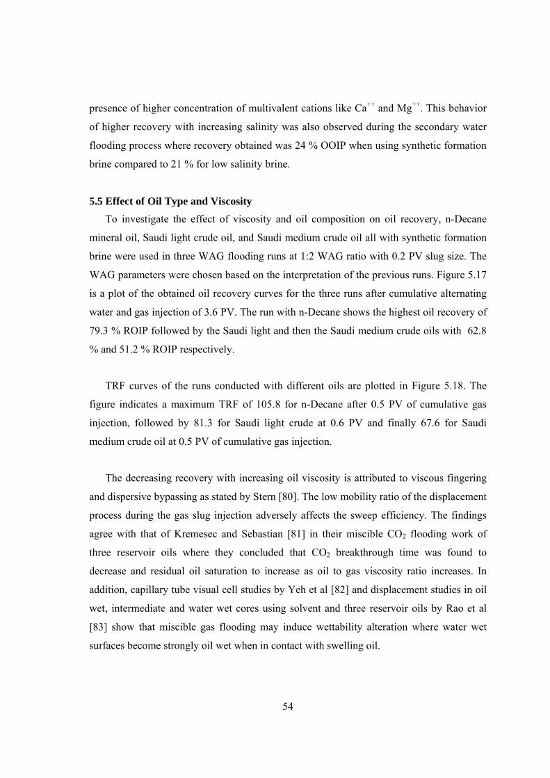
54
presence of higher concentration of multivalent cations like Ca++ and Mg++. This behavior
of higher recovery with increasing salinity was also observed during the secondary water
flooding process where recovery obtained was 24 % OOIP when using synthetic formation
brine compared to 21 % for low salinity brine.
5.5 Effect of Oil Type and Viscosity To investigate the effect of viscosity and oil composition on oil recovery, n-Decane
mineral oil, Saudi light crude oil, and Saudi medium crude oil all with synthetic formation
brine were used in three WAG flooding runs at 1:2 WAG ratio with 0.2 PV slug size. The
WAG parameters were chosen based on the interpretation of the previous runs. Figure 5.17
is a plot of the obtained oil recovery curves for the three runs after cumulative alternating
water and gas injection of 3.6 PV. The run with n-Decane shows the highest oil recovery of
79.3 % ROIP followed by the Saudi light and then the Saudi medium crude oils with 62.8
% and 51.2 % ROIP respectively.
TRF curves of the runs conducted with different oils are plotted in Figure 5.18. The
figure indicates a maximum TRF of 105.8 for n-Decane after 0.5 PV of cumulative gas
injection, followed by 81.3 for Saudi light crude at 0.6 PV and finally 67.6 for Saudi
medium crude oil at 0.5 PV of cumulative gas injection.
The decreasing recovery with increasing oil viscosity is attributed to viscous fingering
and dispersive bypassing as stated by Stern [80]. The low mobility ratio of the displacement
process during the gas slug injection adversely affects the sweep efficiency. The findings
agree with that of Kremesec and Sebastian [81] in their miscible CO2 flooding work of
three reservoir oils where they concluded that CO2 breakthrough time was found to
decrease and residual oil saturation to increase as oil to gas viscosity ratio increases. In
addition, capillary tube visual cell studies by Yeh et al [82] and displacement studies in oil
wet, intermediate and water wet cores using solvent and three reservoir oils by Rao et al
[83] show that miscible gas flooding may induce wettability alteration where water wet
surfaces become strongly oil wet when in contact with swelling oil.
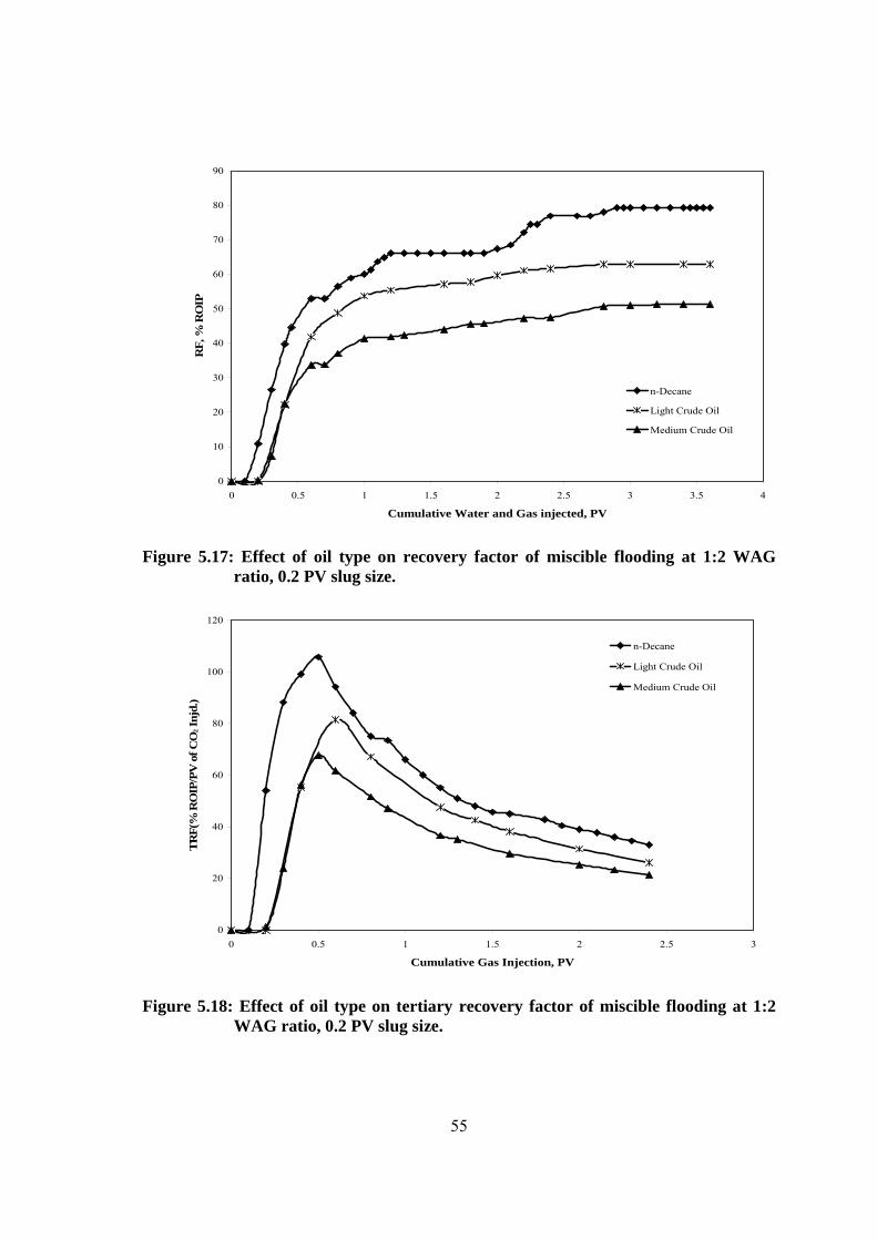
55
0
10
20
30
40
50
60
70
80
90
0 0.5 1 1.5 2 2.5 3 3.5 4
Cumulative Water and Gas injected, PV
RF,
% R
OIP
n-Decane
Light Crude Oil
Medium Crude Oil
Figure 5.17: Effect of oil type on recovery factor of miscible flooding at 1:2 WAG ratio, 0.2 PV slug size.
0
20
40
60
80
100
120
0 0.5 1 1.5 2 2.5 3
Cumulative Gas Injection, PV
TR
F(%
RO
IP/P
V o
f CO
2 Inj
d.)
n-Decane
Light Crude Oil
Medium Crude Oil
Figure 5.18: Effect of oil type on tertiary recovery factor of miscible flooding at 1:2 WAG ratio, 0.2 PV slug size.
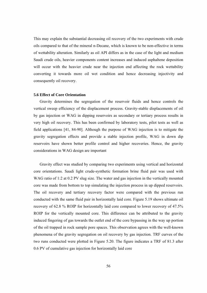
56
This may explain the substantial decreasing oil recovery of the two experiments with crude
oils compared to that of the mineral n-Decane, which is known to be non-effective in terms
of wettability alteration. Similarly as oil API differs as in the case of the light and medium
Saudi crude oils, heavier components content increases and induced asphaltene deposition
will occur with the heavier crude near the injection end affecting the rock wettability
converting it towards more oil wet condition and hence decreasing injectivity and
consequently oil recovery.
5.6 Effect of Core Orientation
Gravity determines the segregation of the reservoir fluids and hence controls the
vertical sweep efficiency of the displacement process. Gravity-stable displacements of oil
by gas injection or WAG in dipping reservoirs as secondary or tertiary process results in
very high oil recovery. This has been confirmed by laboratory tests, pilot tests as well as
field applications [41, 84-90]. Although the purpose of WAG injection is to mitigate the
gravity segregation effects and provide a stable injection profile, WAG in down dip
reservoirs have shown better profile control and higher recoveries. Hence, the gravity
considerations in WAG design are important
Gravity effect was studied by comparing two experiments using vertical and horizontal
core orientations. Saudi light crude-synthetic formation brine fluid pair was used with
WAG ratio of 1:2 at 0.2 PV slug size. The water and gas injection in the vertically mounted
core was made from bottom to top simulating the injection process in up dipped reservoirs.
The oil recovery and tertiary recovery factor were compared with the previous run
conducted with the same fluid pair in horizontally laid core. Figure 5.19 shows ultimate oil
recovery of 62.8 % ROIP for horizontally laid core compared to lower recovery of 47.5%
ROIP for the vertically mounted core. This difference can be attributed to the gravity
induced fingering of gas towards the outlet end of the core bypassing in the way up portion
of the oil trapped in rock sample pore spaces. This observation agrees with the well-known
phenomena of the gravity segregation on oil recovery by gas injection. TRF curves of the
two runs conducted were plotted in Figure 5.20. The figure indicates a TRF of 81.3 after
0.6 PV of cumulative gas injection for horizontally laid core
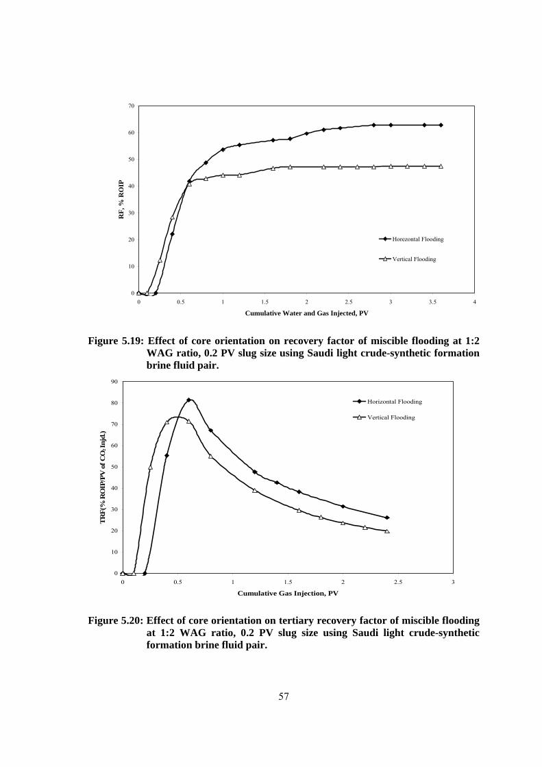
57
0
10
20
30
40
50
60
70
0 0.5 1 1.5 2 2.5 3 3.5 4
Cumulative Water and Gas Injected, PV
RF,
% R
OIP
Horezontal Flooding
Vertical Flooding
Figure 5.19: Effect of core orientation on recovery factor of miscible flooding at 1:2 WAG ratio, 0.2 PV slug size using Saudi light crude-synthetic formation brine fluid pair.
0
10
20
30
40
50
60
70
80
90
0 0.5 1 1.5 2 2.5 3
Cumulative Gas Injection, PV
TR
F(%
RO
IP/P
V o
f CO
2 In
jd.)
Horizontal Flooding
Vertical Flooding
Figure 5.20: Effect of core orientation on tertiary recovery factor of miscible flooding at 1:2 WAG ratio, 0.2 PV slug size using Saudi light crude-synthetic formation brine fluid pair.
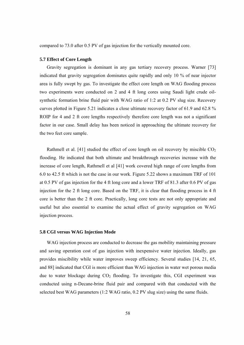
58
compared to 73.0 after 0.5 PV of gas injection for the vertically mounted core.
5.7 Effect of Core Length
Gravity segregation is dominant in any gas tertiary recovery process. Warner [73]
indicated that gravity segregation dominates quite rapidly and only 10 % of near injector
area is fully swept by gas. To investigate the effect core length on WAG flooding process
two experiments were conducted on 2 and 4 ft long cores using Saudi light crude oil-
synthetic formation brine fluid pair with WAG ratio of 1:2 at 0.2 PV slug size. Recovery
curves plotted in Figure 5.21 indicates a close ultimate recovery factor of 61.9 and 62.8 %
ROIP for 4 and 2 ft core lengths respectively therefore core length was not a significant
factor in our case. Small delay has been noticed in approaching the ultimate recovery for
the two feet core sample.
Rathmell et al. [41] studied the effect of core length on oil recovery by miscible CO2
flooding. He indicated that both ultimate and breakthrough recoveries increase with the
increase of core length, Rathmell et al [41] work covered high range of core lengths from
6.0 to 42.5 ft which is not the case in our work. Figure 5.22 shows a maximum TRF of 101
at 0.5 PV of gas injection for the 4 ft long core and a lower TRF of 81.3 after 0.6 PV of gas
injection for the 2 ft long core. Based on the TRF, it is clear that flooding process in 4 ft
core is better than the 2 ft core. Practically, long core tests are not only appropriate and
useful but also essential to examine the actual effect of gravity segregation on WAG
injection process.
5.8 CGI versus WAG Injection Mode
WAG injection process are conducted to decrease the gas mobility maintaining pressure
and saving operation cost of gas injection with inexpensive water injection. Ideally, gas
provides miscibility while water improves sweep efficiency. Several studies [14, 21, 65,
and 88] indicated that CGI is more efficient than WAG injection in water wet porous media
due to water blockage during CO2 flooding. To investigate this, CGI experiment was
conducted using n-Decane-brine fluid pair and compared with that conducted with the
selected best WAG parameters (1:2 WAG ratio, 0.2 PV slug size) using the same fluids.
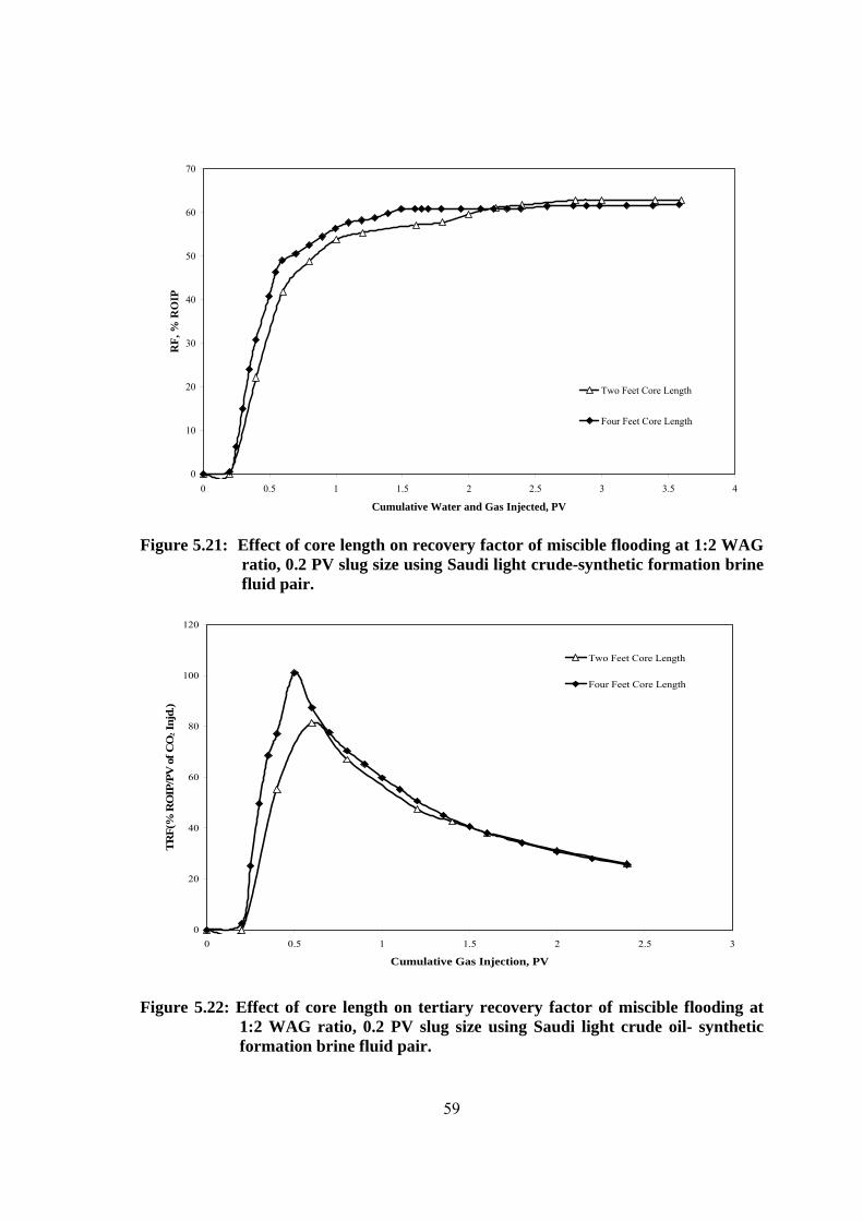
59
0
10
20
30
40
50
60
70
0 0.5 1 1.5 2 2.5 3 3.5 4
Cumulative Water and Gas Injected, PV
RF,
% R
OIP
Two Feet Core Length
Four Feet Core Length
Figure 5.21: Effect of core length on recovery factor of miscible flooding at 1:2 WAG
ratio, 0.2 PV slug size using Saudi light crude-synthetic formation brine fluid pair.
0
20
40
60
80
100
120
0 0.5 1 1.5 2 2.5 3
Cumulative Gas Injection, PV
TR
F(%
RO
IP/P
V o
f CO
2 Inj
d.)
Two Feet Core Length
Four Feet Core Length
Figure 5.22: Effect of core length on tertiary recovery factor of miscible flooding at 1:2 WAG ratio, 0.2 PV slug size using Saudi light crude oil- synthetic formation brine fluid pair.
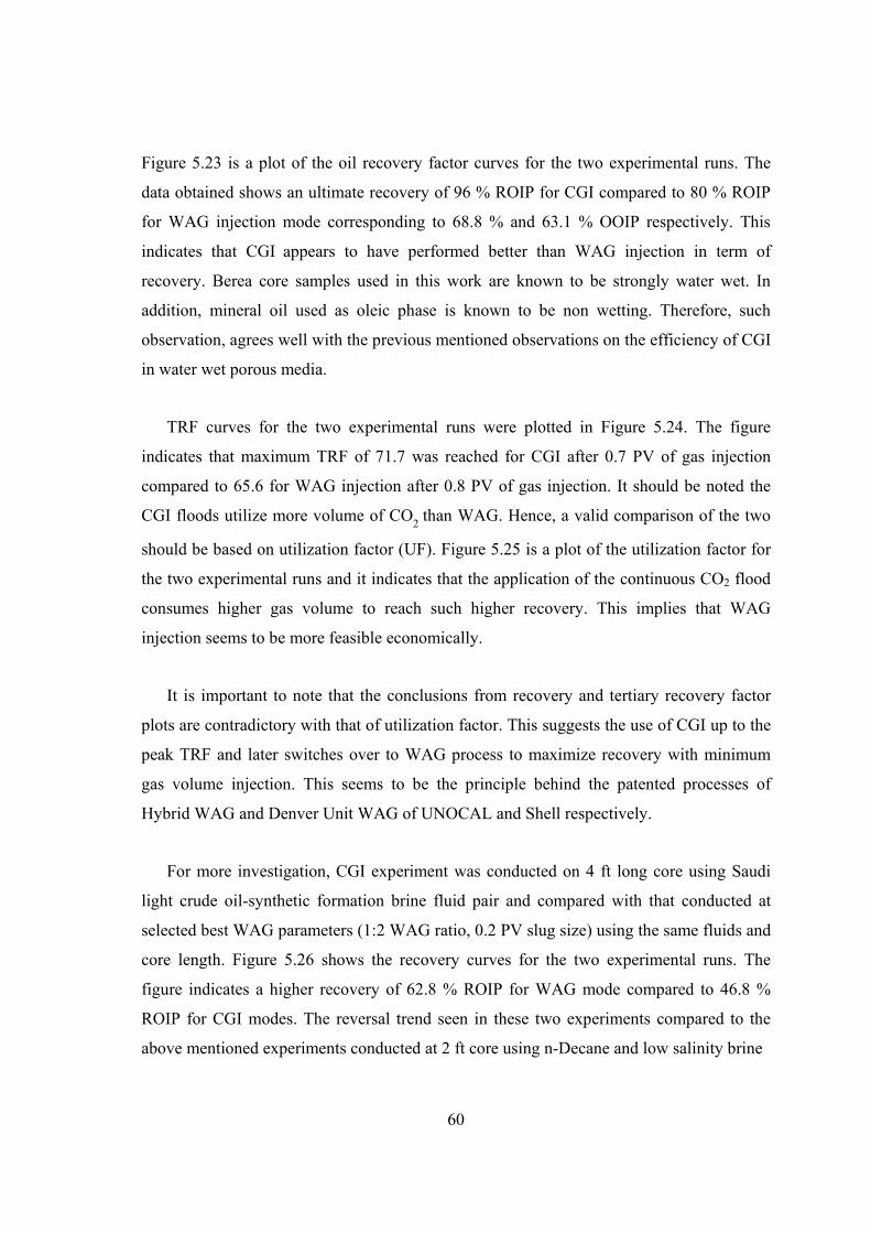
60
Figure 5.23 is a plot of the oil recovery factor curves for the two experimental runs. The
data obtained shows an ultimate recovery of 96 % ROIP for CGI compared to 80 % ROIP
for WAG injection mode corresponding to 68.8 % and 63.1 % OOIP respectively. This
indicates that CGI appears to have performed better than WAG injection in term of
recovery. Berea core samples used in this work are known to be strongly water wet. In
addition, mineral oil used as oleic phase is known to be non wetting. Therefore, such
observation, agrees well with the previous mentioned observations on the efficiency of CGI
in water wet porous media.
TRF curves for the two experimental runs were plotted in Figure 5.24. The figure
indicates that maximum TRF of 71.7 was reached for CGI after 0.7 PV of gas injection
compared to 65.6 for WAG injection after 0.8 PV of gas injection. It should be noted the
CGI floods utilize more volume of CO2 than WAG. Hence, a valid comparison of the two
should be based on utilization factor (UF). Figure 5.25 is a plot of the utilization factor for
the two experimental runs and it indicates that the application of the continuous CO2 flood
consumes higher gas volume to reach such higher recovery. This implies that WAG
injection seems to be more feasible economically.
It is important to note that the conclusions from recovery and tertiary recovery factor
plots are contradictory with that of utilization factor. This suggests the use of CGI up to the
peak TRF and later switches over to WAG process to maximize recovery with minimum
gas volume injection. This seems to be the principle behind the patented processes of
Hybrid WAG and Denver Unit WAG of UNOCAL and Shell respectively.
For more investigation, CGI experiment was conducted on 4 ft long core using Saudi
light crude oil-synthetic formation brine fluid pair and compared with that conducted at
selected best WAG parameters (1:2 WAG ratio, 0.2 PV slug size) using the same fluids and
core length. Figure 5.26 shows the recovery curves for the two experimental runs. The
figure indicates a higher recovery of 62.8 % ROIP for WAG mode compared to 46.8 %
ROIP for CGI modes. The reversal trend seen in these two experiments compared to the
above mentioned experiments conducted at 2 ft core using n-Decane and low salinity brine
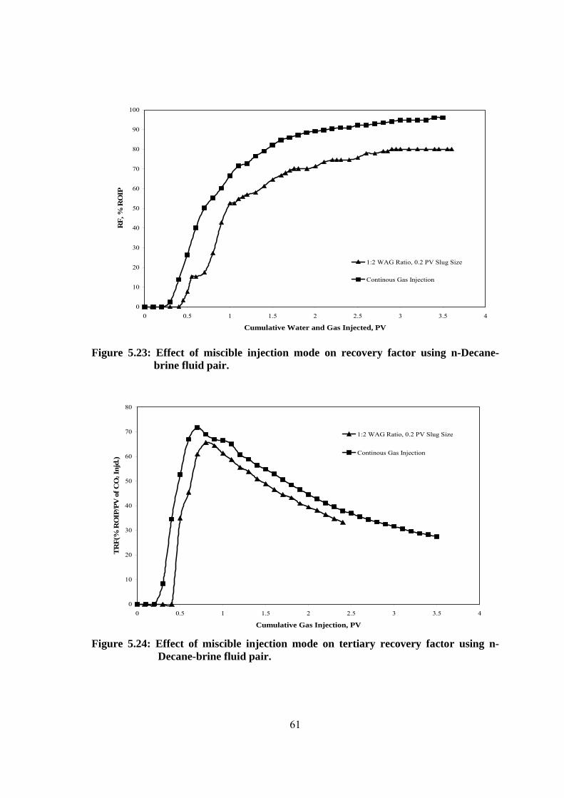
61
0
10
20
30
40
50
60
70
80
90
100
0 0.5 1 1.5 2 2.5 3 3.5 4
Cumulative Water and Gas Injected, PV
RF,
% R
OIP
1:2 WAG Ratio, 0.2 PV Slug Size
Continous Gas Injection
Figure 5.23: Effect of miscible injection mode on recovery factor using n-Decane-
brine fluid pair.
0
10
20
30
40
50
60
70
80
0 0.5 1 1.5 2 2.5 3 3.5 4
Cumulative Gas Injection, PV
TR
F(%
RO
IP/P
V o
f CO
2 Inj
d.)
1:2 WAG Ratio, 0.2 PV Slug Size
Continous Gas Injection
Figure 5.24: Effect of miscible injection mode on tertiary recovery factor using n-
Decane-brine fluid pair.
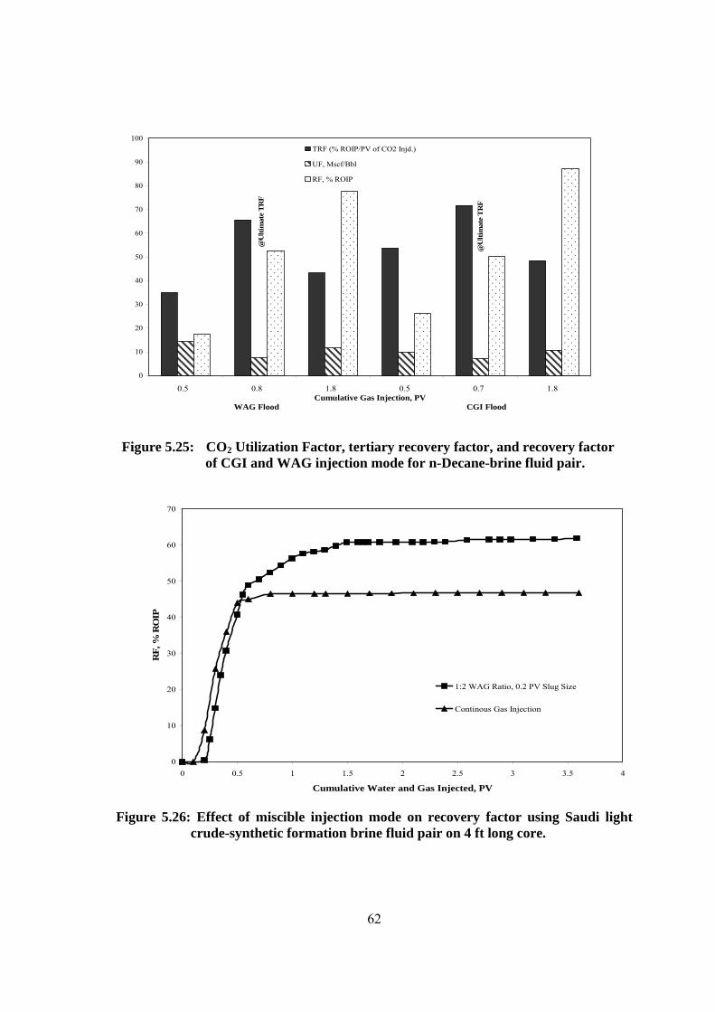
62
0
10
20
30
40
50
60
70
80
90
100TRF (% ROIP/PV of CO2 Injd.)
UF, Mscf/Bbl
RF, % ROIP
@U
ltim
ate
TR
F
@U
ltim
ate
TR
F
0.5 0.8 1.8 0.5 0.7 1.8
Cumulative Gas Injection, PV WAG Flood CGI Flood
Figure 5.25: CO2 Utilization Factor, tertiary recovery factor, and recovery factor
of CGI and WAG injection mode for n-Decane-brine fluid pair.
0
10
20
30
40
50
60
70
0 0.5 1 1.5 2 2.5 3 3.5 4
Cumulative Water and Gas Injected, PV
RF,
% R
OIP
1:2 WAG Ratio, 0.2 PV Slug Size
Continous Gas Injection
Figure 5.26: Effect of miscible injection mode on recovery factor using Saudi light
crude-synthetic formation brine fluid pair on 4 ft long core.

63
fluid pair is due to the effect of the presence of Saudi light crude oil which is believed to
alter the rock wettability towards oil wet condition preventing the water blockage during
the WAG process. TRF curves are plotted in Figure 5.27 and indicate an ultimate TRF of
101 at 0.5 PV of gas injection for WAG injection mode compared to 89.9 % accomplished
after 0.4 PV of gas injection for the CGI mode.
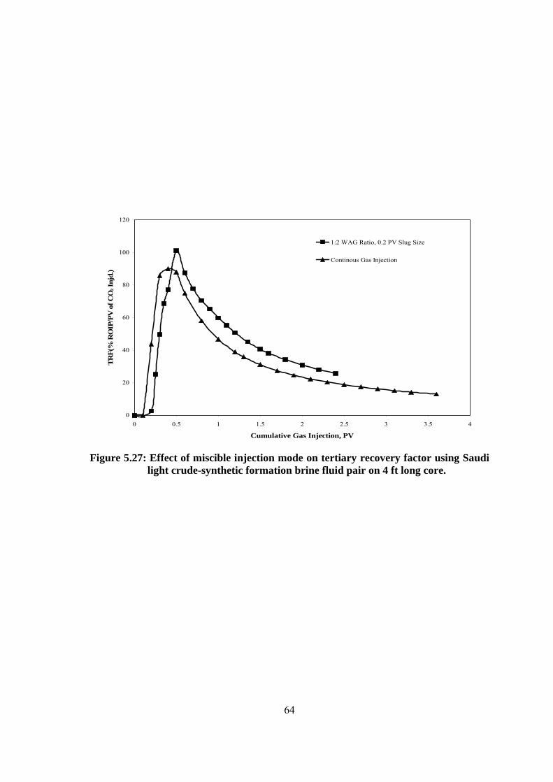
64
0
20
40
60
80
100
120
0 0.5 1 1.5 2 2.5 3 3.5 4
Cumulative Gas Injection, PV
TR
F(%
RO
IP/P
V o
f CO
2 Inj
d.)
1:2 WAG Ratio, 0.2 PV Slug Size
Continous Gas Injection
Figure 5.27: Effect of miscible injection mode on tertiary recovery factor using Saudi
light crude-synthetic formation brine fluid pair on 4 ft long core.
65
CHAPTER 6
CONCLUSIONS AND RECOMMENDATIONS Miscible CO2 flooding process was conducted at different parameters. These
parameters included injection scheme (CGI and WAG), WAG ratio, slug size, oil
composition and viscosity, brine composition, core length and core orientation. In addition,
CO2 flooding as a secondary process was investigated and compared to the conventional
tertiary gas flooding. Based on the results obtained, the following conclusions were drawn:
1. Miscible CO2 flooding experiments at different WAG ratio and slug size show that
1:2 WAG ratio at 0.2 PV slug size is found to be the best combination delivering
the highest recovery and tertiary recovery factors.
2. Comparison of the miscible WAG flooding as a secondary process to the
conventional tertiary miscible WAG flooding process shows that secondary
miscible WAG flooding process is better in term of higher ultimate recovery.
However, secondary WAG requires larger amount of gas injection particularly in
the early injection process, this may be attributed to the less water saturation
present as connate water compared to the higher water saturation accumulated
subsequent to the normal water flooding secondary process.
3. Equal ultimate recovery were obtained for the miscible WAG experiments
conducted at the best flooding scenario with different brine composition and
concentration with some delay in approaching that recovery when using the low
salinity brine solution. An increase in the tertiary recovery factor and slight
decrease in the UF was noticed as we switch from low to high salinity brine.
4. As the oleic phase API decreases and the viscosity increases, recovery factor and
tertiary recovery factor decreases due to wettability alteration and viscose fingering
for both miscible and immiscible injection modes.
5. Gravity determines the segregation of the reservoir fluids and hence controls the
vertical sweep efficiency of the displacement process. Gravity-stable
displacements of oil by miscible WAG injection in vertically mounted core
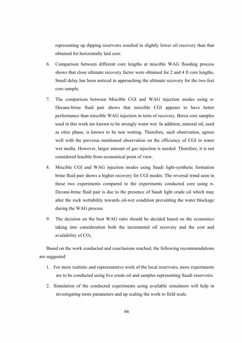
66
representing up dipping reservoirs resulted in slightly lower oil recovery than that
obtained for horizontally laid core.
6. Comparison between different core lengths at miscible WAG flooding process
shows that close ultimate recovery factor were obtained for 2 and 4 ft core lengths.
Small delay has been noticed in approaching the ultimate recovery for the two feet
core sample.
7. The comparison between Miscible CGI and WAG injection modes using n-
Decane-brine fluid pair shows that miscible CGI appears to have better
performance than miscible WAG injection in term of recovery. Berea core samples
used in this work are known to be strongly water wet. In addition, mineral oil, used
as oleic phase, is known to be non wetting. Therefore, such observation, agrees
well with the previous mentioned observation on the efficiency of CGI in water
wet media. However, larger amount of gas injection is needed. Therefore, it is not
considered feasible from economical point of view.
8. Miscible CGI and WAG injection modes using Saudi light-synthetic formation
brine fluid pair shows a higher recovery for CGI modes. The reversal trend seen in
these two experiments compared to the experiments conducted core using n-
Decane-brine fluid pair is due to the presence of Saudi light crude oil which may
alter the rock wettability towards oil-wet condition preventing the water blockage
during the WAG process.
9. The decision on the best WAG ratio should be decided based on the economics
taking into consideration both the incremental oil recovery and the cost and
availability of CO2
Based on the work conducted and conclusions reached, the following recommendations
are suggested:
1. For more realistic and representative work of the local reservoirs, more experiments
are to be conducted using live crude oil and samples representing Saudi reservoirs.
2. Simulation of the conducted experiments using available simulators will help in
investigating more parameters and up scaling the work to field scale.

67
3. Hybrid-WAG flooding should be conducted on long cores to determine the
optimum mode for gas floods and to compare their effectiveness against gravity-
stable gas floods.
NOMENCLATURE
ANN : Artificial Neural Network
API : oil gravity °API
Ci : carbon number
Exp. No. : experiment numbers
F : weighting composition parameter
FR : mole percent C2 through C6 in the reservoir fluid, %
Interm. : intermediates components, C1-C4, H2S, and CO2, fraction
Ki : normalized partition coefficient for carbon number i.
MFi : critical temperature modification factor of injected gas component i.
Minj. : molecular weight of the injected gas
MMPpure : CO2-oil Minimum Miscibility Pressure, MPa
MMPimpure : Flue gas-oil Minimum Miscibility Pressure, MPa
MWC5+ : molecular weight of C5+ fraction
MWC7+ : molecular weight of C7+ fraction
PC, pure : CO2 critical pressure, MPa
PCi : critical pressure of the gas component i, MPa
PC, inj. : injection gas critical pressure, MPa
PCW : weight average pseudocritical pressure, MPa
Pr, pure : reduced CO2 minimum miscibility pressure, fraction
Pr, impure : reduced flue gas minimum miscibility pressure, fraction
SFi : Dong (1999) factor representing the strength of species i in changing
the apparent critical temperature of the mixture relative to the critical
temperature of CO2
Tac : mole average pseudocritical temperature with using factor SFi, °K
TC, CO2 : critical temperature of pure CO2 gas, °C
TC, inj. : injected gas critical temperature, °K
Tci : critical temperature of gas component i, °C
TCi : critical temperature of gas component i, °K
TCM : mole average critical temperature, °K
TCW : weight average pseudocritical temperature with using the Multiplying
...factor (MFi), °C
Tpc : Pseudocritical temperature (may be weight average or mole average),
°C
TR : reservoir temperature, °C
Vol. : volatiles (C1 and N2) mole percentage, %
wi : weight fraction of gas component i
wic2+ : component i normalized weighting fraction in the C2+ fractions of
crude ..oil
xCO2 : CO2 mole percentage in the injection gas, %
xi : mole fraction of gas component i
y : mole fraction of diluted component
ρ : oil gravity °API
ρMMP : CO2 density at MMP, g/cm3
Σ : sum operator
REFERENCES
1. Benson S. and Peter Cook, “Carbon Dioxide Capture and Storage”, Chapter 5,
Intergovernmental Panel on Climate Change Report, Cambridge University Press,
2005.
2. Oen, P. M., “The Development of the Greater Gorgon Gas Fields”, The APPEA
Journal, 43(2), pp.167–177, 2003.
3. Van der Meer, L.G.H.; Hartman, J.; Geel, C.; and E. Kreft, “Re-injecting CO2
into an Offshore Gas Reservoir at a Depth of Nearly 4000 metres Sub-Sea”,
Proceedings of the 7th International Conference on Greenhouse Gas Control
Technologies (GHGT-7), September 5–9, Vancouver, Canada, Vol. I, 521-530,
2004.
4. Bachu, S. and Haug, K., “In-Situ Characteristics of Acid –Gas Injection
Operations in the Alberta Basin, Western Canada: Demonstration of CO2
Geological Storage, Carbon Dioxide Capture for Storage in Deep Geologic
Formations – Results from the CO2 Capture Project, v. 2: Geologic Storage of
Carbon Dioxide with Monitoring and Verification”, S.M. Benson (ed.), Elsevier,
London, pp. 867–876, 2005.
5. Freund, P., “Progress in Understanding the Potential Role of CO2 Storage”,
Proceedings of the 5th International Greenhouse Gas Conference Technologies
(GHGT5), Cairns, Australia, 13–16 August, pp. 272–278, 2000.
6. Stevens, S.H.; Kuuskraa, V.K.; and Gale, J., “Sequestration of CO2 in Depleted
Oil and Gas Fields: Global Capacity and Barriers to Overcome”, Proceedings of
the 5th International Greenhouse Gas Conference Technologies (GHGT5),
Cairns, Australia, 13–16 August, 2000.
7. Gozalpour, F., Ren, S. R. , Tohidi, B., “CO2 EOR and Storage in Oil Reservoirs”
Oil & Gas Science and Technology – Rev. IFP, Vol. (60) , No. 3, pp. 537-546,
2005.
8. Moberg, R.; Stewart, D.B.; and Stachniak, D., “The IEA Weyburn CO2
Monitoring and Storage Project. Proceedings of the 6th International Conference
on Greenhouse Gas Control Technologies (GHGT-6), J. Gale and Y. Kaya (eds.),
Kyoto, Japan, 219–224, 1–4 October 2002.
9. Law, D., “Theme 3: CO2 Storage Capacity and Distribution Predictions and the
Application of Economic Limits. In: IEA GHG Weyburn CO2 Monitoring and
Storage Project Summary Report 2000–2004, M. Wilson and M. Monea (eds.),
Proceedings of the 7th International Conference on Greenhouse Gas Control
Technologies (GHGT7), Volume III, p 151–209, 2005.
10. Moritis, G. “CO2 Sequestration Adds New Dimension to Oil, Gas Production”.
Oil and Gas Journal, 101(9), pp. 71–83, 2003.
11. Holt, T.; Jensen, J. L.; and Lindeberg, E., “Underground Storage of CO2 in
Aquifers and Oil Reservoirs”, Energy Conversion and Management, 36(6–9), pp.
535–538, 1995.
12. Bondor, P.L., “Applications of Carbon Dioxide in Enhanced Oil Recovery”.
Energy Conversion and Management, 33(5), pp. 579–586, 1992.
13. Martin, F.D. and Taber, J. J., “Carbon Dioxide Flooding”, Journal of Petroleum
Technology, 44(4), pp. 396–400, 1992.
14. Stalkup Jr., F.I., “Miscible Displacement. SPE Monograph Series,” New York,
pp. 12-14, 1983.
15. Sequeira, D. S., “Compositional Effects on Gas-Oil Interfacial Tension and
Miscibility at Reservoir Conditions” Dissertation, Petroleum Engineering Dept.,
Louisiana State University, December 2006.
16. Tzimas, E.; Georgakaki, A., Garcia Cortes, C. and Peteves, S.D. “Enhanced Oil
Recovery using Carbon Dioxide in the European Energy System” Report EUR
21895 EN, Institute for Energy, Petten, The Netherlands, December 2005.
17. Goodwear, S.G., “Subsurface Issues for CO2 Flooding of UKCS Reservoirs”
Trans. Ichem E, 81, Part A, 2003.
18. Moritis, G., “2000 Worldwide EOR Survey”, Oil & Gas J., 45, March 2000.
19. Green, D.W. and Willhite, G.P., ‘’Enhanced Oil Recovery,’’ Society of
Petroleum Engineers, SPE Textbook Series Vol. 6, Richardson, TX, USA, 2003.
20. Shokir, E.M. El-M., “CO2-Oil Minimum Miscibility Pressure Model for Impure
and Pure CO2 Streams” Journal of Petroleum Science and Technology, (58), pp.
173–185, 2007.
21. Taber, J.J.; Martin, F.D.; and Seright; R.S., “EOR Screening Criteria Revisited -
part 1: Introduction to Screening Criteria and Enhanced Recovery Fields
Projects’’, SPE Reservoir Engineering, 12(3), pp. 189–198, 1997.
22. Kovscek, A.R., “Screening Criteria for CO2 Storage in Oil Reservoirs”,
Petroleum Science and Technology, 20(7–8), pp. 841–866, 2002.
23. Shaw, J. C. and S. Bachu, “Screening, Evaluation and Ranking of Oil Reserves
Suitable for CO2 Flood EOR and Carbon Dioxide Sequestration”, Journal of
Canadian Petroleum Technology, 41(9), pp. 51–61, 2002.
24. Wang, Y., “Analytical Calculation of Minimum Miscibility Pressure,”
Dissertation for PhD degree, Stanford University, Department of Petroleum
Engineering USA, 1998.
25. Kovarik, F. S., “A minimum Miscibility Pressure Study Using Impure CO2 and
West Texas oil systems: Data Base, Correlations, and Compositional Simulation,”
Paper SPE 14689 presented at the SPE Production Technology Symposium,
Lubbock, Texas, USA, pp. 1-14, Nov. 1985.
26. Benham, A. L.; Dowden, W. E.; and Kunzman, W. J., “Miscible Fluid
Displacement Prediction of Miscibility,” JPT, pp. 229-237, Oct. 1960.
27. Holm, L. W.; and Josendal, V. A, “Effect of Oil Composition on Miscible-Type
Displacement by Carbon Dioxide”, SPE J., pp. 87-98, Feb.1982.
28. Johnson, J. P.; and Pollin, J. S., “Measurement and Correlation of CO2 Miscibility
Pressures,” SPE 9790, presented at the 1981 SPE/DOE Joint Symposium on
Enhanced Oil Recovery held in Tulsa, Oklahoma, April 5-8, 1981.
29. Sebastian, H. M.; Wenger, R. S.; and Renner, T. A., “Correlation of Minimum
Miscibility Pressure for Impure CO2 Streams,” Paper SPE 12648 presented at the
1984 SPE/DOE Symposium on Enhanced Oil Recovery, Tulsa, OK, Apr. 15-18.
30. Flock, D. L.; and Nouar, A., “Parameter Analysis on The Determination of The
Minimum Miscibility Pressure in Slim Tube Displacements,” Journal of Canadian
Pet. Tech., pp. 80-88, Sept-Oct. 1984.
31. Kuo, S. S., “Prediction of Miscibility for The Enriched-Gas,” Paper SPE 14152,
presented at the SPE Annual Technical Conference and Exhibition, Las Vegas,
USA, Sept. 1985.
32. Elsharkawy, A. M.; Poettmann, F. H.; and Christiansen, R.L., “Measuring
Minimum Miscibility Pressure: Slim-Tube or Rising-Bubble Method?,” Paper
SPE 24114 presented at the 1992 SPE/DOE Eighth Symposium on Enhanced Oil
Recovery, Tulsa, OK, April 22-24.
33. Zhou, D.; and Orr, F. M. Jr., “An analysis of Rising Bubble Experiments to
Determine Minimum Miscibility Pressures,” Paper SPE 30786 presented at the
1995 SPE Annual Technical Conference and Exhibition, Dallas, TX, Oct. 22-25,
1995.
34. Lake, L. W., “Enhanced Oil Recovery,” Prentice Hall, New Jersey, 1989.
35. R. L. Christiansen; and K. H. Haines, “Rapid measurement of minimum
miscibility pressure using the rising bubble apparatus,” SPE Reservoir
Engineering Journal, pp. 523-527, Nov. 1987.
36. Dong, M.; Huang, S.; Dyer, S. B.; and Mourits, F. M., “A comparison of CO2
Minimum Miscibility Pressure Determinations for Weyburn Crude Oil,” Journal
of Petroleum Science and Engineering, Vol. 31, No. 1, pp. 13–22, 2001.
37. Johnson, J. P.; and Pollin, J. S., “Measurement and Correlation of CO2 Miscibility
Pressures,” Paper SPE 9790 presented at the SPE/DOE Second Joint Symposium
on Enhanced Oil Recovery, Tulsa, USA, pp. 269-281, 1981.
38. Alston, R. B.; Kokolis, G. P.; and James, C. F., “CO2 Minimum Miscibility
Pressure: A correlation for Impure CO2 Streams and Live Oil Systems,” SPEJ,
Vol. 25, No. 2, pp. 268– 274, 1985.
39. Zuo, Y.; Chu, Ji.; Ke, S.; and Guo, T., “A study on The Minimum Miscibility
Pressure for Miscible Flooding Systems,” Journal of Petroleum Science and
Engineering, Vol. 8, No. 3, pp. 315-328, 1993.
40. Emera, M. K; and Sarma, H. K., “Genetic Algorithm (GA)–Based Correlations
Offer More Reliable Prediction of Minimum Miscibility Pressures (MMP)
between The Reservoir Oil and CO2 or Flue Gas,” Paper presented at 6th
Canadian International Petroleum Conference, Calgary, Alberta, Canada, pp. 1-
17, June 2005.
41. Rathmell, J. J.; talkup, F. I. S; and Hassinger, R. C., “A laboratory Investigation
of Miscible Displacement by Carbon Dioxide,” Paper SPE 3483 presented at the
46th Annual Fall Meeting of the Society of Petroleum Engineers of AIME 6200,
New Orleans, La., pp. 1-16, 1971.
42. Metcalfe, R. S.; and Yarborough, L., “Discussion,” JPT, pp. 1436–1437, Dec.
1974.
43. Cronquist, C., “Carbon Dioxide Dynamic Displacement with Light Reservoir
Oils,” Proc., Fourth Annual U.S. DOE Symposium, Tulsa, USA, pp. 18-23, Aug.
1978.
44. Holm, L. W.; and Josendal, V. A., “Mechanisms of Oil Displacement by Carbon
Dioxide,” JPT, pp1427-1436, Dec. 1974.
45. Lee, J. I., “Effectiveness of Carbon Dioxide Displacement Under Miscible and
Immiscible Conditions,” Report RR-40, Petroleum Recovery Inst., Calgary,
March 1979.
46. Yellig, W. F.; and Metcalfe, R. S., “Determination and Prediction of CO2
Minimum Miscibility Pressures,” JPT, pp. 160– 168, Jun.1980.
47. Orr, F. M. Jr.; and Jensen, C. M., “Interpretation of Pressure-Composition Phase
Diagrams for CO2/Crude-OilSsystems,” SPE Journal, pp. 485-497, Oct. 1984.
48. Glaso, O., “Generalized Minimum Miscibility Pressure Correlation,” SPEJ, pp.
927– 934, Dec. 1985.
49. Orr, F. M. Jr.; and Silva, M. K., “Effect of Oil Composition on Minimum
Miscibility Pressure-Part 2: Correlation,” SPE Reservoir Engineering Journal,
Vol. 2, No. 4, pp. 479– 491, 1987.
50. Huang, H. F.; Huang, G. H.; Dong, G. M.; and Feng, G. M., “Development of an
Artificial Neural Network Model for Predicting Minimum Miscibility Pressure in
CO2 Flooding,” Journal of Petroleum science and Engineering, Vo., 37, No., pp.
83-95, 2003.
51. Emera, M. K.; and Sarma, H. K., “Use of Genetic Algorithm to Estimate CO2-Oil
Minimum Miscibility Pressure-a Key Parameter in Design of CO2 Miscible
Flood,” Journal of Petroleum science and Engineering, Vol. 46, No. 1, pp. 37-52,
2004.
52. Dong, M., “Task 3- Minimum Miscibility Pressure (MMP) Studies, in the
Technical Report: Potential of Greenhouse Storage and Utilization through
Enhanced Oil Recovery,” Petroleum Research Center, Saskatchewan Research
Council (SRC Publication No. P-10-468-C-99), 1999.
53. Eakin, B. E.; and Mitch, F. J., “Measurement and Correlation of Miscibility
Pressures of Reservoir Oils,” Paper SPE 18065 presented at 63rd Annual
Technical Conference and Exhibition, Houston, TX, pp. 75-81, Oct. 1988.
54. Yuan, H.; Johns, R. T.; Egwuenu, A. M.; and Dindoruk, B., “Improved MMP
Correlations for CO2 Floods Using Analytical Gas Flooding Theory,” Paper SPE
89359 presented at the SPE/DOE Fourteenth Symposium on Improved Oil
Recovery, Tulsa, USA, pp. 1-16, Apr. 2004.
55. Rivas, O.; Embid, S.; and Bolivar, F., “Ranking Reservoirs for Carbon Dioxide
Flooding Processes” SPE Advanced Technology Series J., Volume 2, Number 1,
pp. 95-103, March 1992.
56. Gale, J.J., “Opportunities for Early Applications of CO2 Sequestration
Technology”, IEA Greenhouse Gas R&D Program File Note, 2003.
57. Caudle, B.H and Dyes, A.B., “Improving Miscible Displacement by Gas-Water
Injection”, Trans., AIME, pp. 213, 281, 1958.
58. Huang, E.T.S. and Holm, L.W., “Effect of WAG Injection and Rock Wettability
on Oil Recovery During CO2 Flooding”, SPE Reservoir Engineering, 119,
February 1988.
59. Christensen, J R; Stenby, E H; and Skauge, A., “Review of the WAG Field
Experience”, paper SPE 71203 presented at the 1998 SPE International
Petroleum Conference and Exhibition of Mexico, Villa Hermosa, 3-5 March.
60. Pariani, G.J.; McColloch, K.A.; and Warden, S.L., “An Approach To Optimize
Economics in a West Texas CO2 Flood”, JPT, 984; Trans., AIME, 293,
September 1992.
61. Surguchev, L.M.; Korbol, R.; and Krakstad, O.S., “Optimum Water Alternate
Gas Injection Schemes for Stratified Reservoir,” paper SPE 24646 presented at
the 1992 Annual Technical Conference and Exhibition, Washington, DC, 4–7
October.
62. Roper, M.K. Jr. and Pope, G.A., “Analysis of Tertiary Injectivity of Carbon
Dioxide”, paper SPE 23974 presented at the 1992 SPE Permian Basin Oil and
Gas Recovery Conference, Midland, Texas, 18–20 March.
63. Bellavance, J.F.R., “Dollarhide Devonian CO2 Flood: Project Performance
Review 10 Years Later”, paper SPE 35190 presented at the 1996 SPE Permian
Basin Oil and Gas Recovery Conference, Midland, TX, 27-29 March.
64. Farouq Ali, The Unfulfilled Promise of Enhanced Oil Recovery – More Lies
Ahead? SPE London Section Presentation, 30 Sept. 2003.
65. Jackson, D.D.; Andrews, G.L.; and Claridge, E.L., “Optimum WAG Ratio vs.
Rock Wettability in CO2 Flooding”, paper SPE 14303 presented at the 1985
Annual Technical Conference and Exhibition, Las Vegas, NV, 22-25 September.
66. Quijada, M. G., “Optimization of A CO2 Flood Design Wasson Field-West
Texas” Dissertation, Texas A&M University, August 2005.
67. Gharbi, R. B.C., “Integrated Reservoir Simulation Studies to Optimize Recovery
from a Carbonate Reservoir”, paper SPE 80437 presented at the SPE Asia Pacific
Oil and Gas Conference and Exhibition, Jakarta, Indonesia, 9-11 September.
68. Holm, W. L., ‘’Evolution of the Carbon Dioxide Flooding Processes’’, Oil and
Gas Journal, 1337, November 1987.
69. Lin, E.C; and Poole, E.S., “Numerical Evaluation of Single-Slug, WAG, and
Hybrid Con injection Processes, Dollarhide Devonian Unit, Andrews county,
Texas” SPE Reservoir Engineering, November 1991
70. Shedid A. S.; Almehaideb, R.A.; and Zekri, A. Y. “Microscopic Rock
Characterization and Influence of Slug Size on Oil Recovery by CO2 Miscible
Flooding in Carbonate Oil Reservoir,” The Seventh Annual U.A.E. University
Research Conference, UAE.
71. Al-Shehri, D. A., “Carbon Dioxide Minimum Miscibility Pressure for Saudi
Arabian Crudes”, MS.c. thesis, KFUPM, (KSA), 1987.
72. Rappaport, L A., and Leas, W J, “Properties of Linear Waterfloods”, Trans.
AIME (198), pp. 139, 1953.
73. Warner, H.R. Jr., “An Evaluation of Miscible CO2 Flooding in Waterflooded
Sandstone Reservoirs” paper SPE 6117 was presented at the Society of Petroleum
Engineers AIME 51th Annual Fall Technical Conference and Exhibition held in
New Orleans, Oct. 3-6, 1976.
74. Mohanty, K. K., ‘’ Development of Shallow Viscous Oil Reservoirs in North
Slope’’ report no. PE-FC26-01EC15186 reported to US development of energy,
July, 2003.
75. Kwan, M Y.; Cullen, M P.; Jamieson, P R; and Fortier, R A, “A Laboratory Study
of Permeability Damage to Cold Lake Tar Sands Cores”, Journal of Canadian
Petroleum Technology, Vol. 28 (1), pp. 56-62, Jan-Feb 1989.
76. Jones, F O, “Influence of Chemical Composition of Water on Clay Blocking of
Permeability”, SPE 631, Journal of Petroleum Technology, 441-446, April 1964.
77. Khilar, K C.; Vaidya, R N.; and Fogler, H S, “Colloidally - Induced Fines
Release in Porous Media”, Journal of Petroleum Technology, vol. 4, pp. 213 –
221, July 1990.
78. Tang, G.; and Morrow, N R, “Oil Recovery by Waterflooding and Imbibitions –
Invading Brine Cation Valency and Salinity”, SCA 9911 Proceedings of the
International Symposium of the Society of Core Analysts, Golden, CO, August
1999.
79. Filoco, P R.; and Sharma, M M, “Effect of Brine Salinity and Crude-Oil
Properties on Oil Recovery and Residual Oil Saturations”, SPE 65402, Presented
at 1998 SPE Annual Technical Conference and Exhibition, held in New Orleans,
LA 27-30 Sept. 1998.
80. Stern, D.: “Mechanisms of Miscible Oil Recovery: Effects of Pore- Level Fluid
Distribution,” paper SPE 22652 presented at the 1991 SPE Annual Technical
Conference and Exhibition, Dallas, 6–9 October.
81. Kremesec, Jr. V.J.; and Sebastian, H.M., “CO2 Displacements of Reservoir Oils
From Long Berea Cores: Laboratory and Simulation Result,” Paper SPE 14306,
May 1988.
82. Yeh, S.W.; Ehrlich, R.; and Emanuel, A.S.: “Miscible Gas flood Induced
Wettability Alteration: Experimental Observations and Oil Recovery
Implications,” SPEFE (167), June 1992.
83. Rao, D.N.; Girard, M.; and Sayegh, S.G., “Impact of Miscible Flooding on
Wettability, Relative Permeability, and Oil Recovery,” SPERE (204), May 1992.
84. Bangla, V K.; and Yau, F.; and Hendricks, G R, “Reservoir Performance of a
Gravity Stable Vertical CO2 Miscible Flood: Wolfcamp Reservoir, Wellman
Unit”, SPE 22898, presented at the 66th annual technical conference and
exhibition of the Society of Petroleum Engineers, held in Dallas, TX, Oct 6-9,
1991.
85. Tiffin, D L., and Kremesec, V J, “A mechanistic Study of Gravity-Assisted
Flooding”, SPE/DOE 14895, presented at the SPE/DOE fifth symposium on
Enhanced oil recovery of the Society of Petroleum Engineers and the Department
of Energy, held in Tulsa, OK, April 20-23, 1986.
86. Karim, F.; Berzins, T V.; Schenewerk, P.A.; Bassiouni, Z A.; and Wolcott, J M,
“Light Oil Recovery from Cyclic Injection: Influence of Drive Gas, Injection
Rate and Reservoir Dip’’, SPE 24336, presented at SPE rocky mountain regional
meeting held in Casper, Wyoming, May 18-21, 1992.
87. Thomas, J.; Berzins, T. V.; Monger, T. G.; and Bassiouni, Z. A., “Light Oil
Recovery from Cyclic CO2 Injection: Influence of Gravity Segregation and
Remaining Oil”, SPE 20531, presented at the 65th Annual Technical Conference
and Exhitition of the society of petroleum Engineers helo in New Orleans, LA,
September 23-26, 1990
88. Raimondi, P.; and Torcaso, M.S., “Mass Transfer between Phases in a Porous
Medium: A Study of Equilibrium”, SPEJ (51), March 1965.
89. Righi, E.F.; Royo, J.; Gentil, P.; Castelo, R.; and Monte, A.D. “Experimental
Study of Tertiary Immiscible WAG Injection’’, Paper SPE 89360, SPE/DOE
Symposium on Improved Oil Recovery, Tulsa, Oklahoma, 17-21 April 2004.
90. Mangalsingh, D.; and Jagai, T., ‘’A Laboratory Investigation of the Carbon
Dioxide Immiscible Process’’, Paper SPE 36134, SPE Latin America/Caribbean
Petroleum Engineering Conference Port-of-Spain, Trinidad, 23-26 April 1996.

Engineer: Ali Suleman Al-Netaifi
KSA, Riyadh
P.O. Box: 90582 Riyadh 11623
Tel. (Office): +966-1-4676883
Tel. (Home): +966-1-4561396
Tel. (Mobil): +966-555244970
Fax : +966-1-4674422
E-mail: [email protected]

ملخص الرسالة
ات ة آلي ق ثالث ة الغمر اإلمتزاجي تحدث عن طري ام بطريق ات تكمن في . إن الزيادة في إنتاج الزيت الخ ذه األلي ه
ل ) غاز ثاني أآسيد الكربون (إزاحة الزيت بواسطة المذيب ام، وتقلي اخ الزيت الخ عبر إمتزاج للغاز بالزيت الخام، وإنتف
.لزوجة الزيت الخام
ي ذات أطوال عمليات الغمر المتتابع للغاز والماءلتقييم أداء تم إجراء تجارب معملية على عينات من الصخر الرمل
ة دم، 2(مختلف دم4ق ة ) ق وت مختلف تخدام زي ة، وإس ز مختلف ة ذات تراآيب وتراآي ة مائي ل ملحي تخدام محالي ديكان (بإس ال
ة ). م متوسط الكثافة الطبيعي، والزيت السعودي الخام الخيفيف، والزيت السعودي الخا ولقد تم دراسة تأثير آال من نوعي
از (ضخ الغاز ة الغمر المتواصل للغ ابع، )في حالة الغمر المتتابع للغاز والماء، وفي حال از المتت اء للغ سبة ضخ الم ، ون
صخرية ة ال از للعين ن الغ اه حق ستخدم، وإتج وع الزيت الم اء، ون از والم ، ) و أفقي عمودي ( وحجم الجبهه المحقنة للغ
از ام بالغ ت الخ ي للزي اج الثالث ل اإلنت ام ومعام ت الخ اج للزي ل اإلنت ى معام ستخدمة عل صخرية الم ات ال ول العين . وط
ة ة ثالثي ة وآعملي از ( وباإلضافة إلى ذلك تمت مقارنة إنتاجية آل من الغمر المتتابع للغاز والماء آعملية ثنائي ن الغ )لحق
. عند نفس الظروف
ة 2:1 نتائج تجارب الغمر اإلمتزاجي الثالثي للزيت الخام بالغاز أن نسبة الماء للغاز لقد أثبتت ة المحقن م الجبه وحج
اج هما أفضل عوامل للغمر المتتابع 0¸2للغاز والماء المتتابع للغاز والماء حيث أدت هذه العوامل إلى أفضل معامل إنت
ي المراحل وب. وأفضل معامل إنتاج ثالثي لزيت الخام بالغاز ستهلك خاصة ف ون ي از المحق التالي فإن آمية آبيرة من الغ
.األولى لعملية الحقن
ة الزيت د آثاف دما تزي ل عن از يق ام بالغ ي لزيت الخ اج الثالث اج ومعامل اإلنت أي (ولقد ثبت أن آًال من معامل اإلنت
از نتيجة ويعتقد أن هذا يرجع إلى تغير خاصية تبلل الصخر الرم ) APIعندما تنخفض لي، وأيضًا إلى سرعة خروج الغ
ام ). Viscous Fingering(إلى إختالف اللزوجة مابين الزيت الخام والغاز ائي للزيت الخ وثبت أن معامل اإلنتاج النه
ة ل اإلنتاجي ي معام أخير ف دث بعض الت د يح ه ق ز إال أن ب والترآي ة الترآي ة مختلف ل مائي تخدام محالي د إس ساوى عن يت
ل . المحلول المائي منخفض الملوحة بإستخدام وهذه النتيجة أدت إلى زيادة معامل اإلنتاج الثالثي للزيت بالغاز وأيضًا تقلي
.معامل إستهالك غاز ثاني أآسيد الكربون نسبيًا في حالة زيادة ملوحة المحلول المائي
ماء في اإلتجاه العمودي يكون أقل نسبيًا من إن معامل إنتاج الزيت الخام في حالة الغمر اإلمتزاجي المتتابع للغاز وال
ي اه األفق ي اإلتج اء ف از والم ابع للغ ر المتت ة الغم اء . حال از والم ابع للغ ر اإلمتزاجي المتت ائج الغم ة نت ة مقارن ي حال وف
دم، 2(بإسخدام عينات صخرية مختلفة الطول دم 4ق و ) ق ه ل التين، إال أن ا الح ساوى في آلت اج يت حظ وجد أن معامل اإلنت
).قدم2(بعض التأخير في معامل اإلنتاج في حالة إستخدام العينات الصخرية القصيرة

ديكان الطبيعي يكون ون وبإسخدام ال سيد الكرب إن معامل اإلنتاج في حالة الغمر اإلمتزاجي المتواصل بغاز ثاني أآ
ا أفضل من معامل إنتاج الزيت الخام في حالة الغمر اإلمتزاجي المتتابع للغاز و ى أن صخور البيري ك إل الماء، ويرجع ذل
ستخدم . المستخدمة في هذا البحث معروف عنها أنها شديدة التبلل بالماء ى أن الزيت الم ديكان الطبيعي (وباإلضافة إل ) ال
اءة الغمر ى آف شير إل ى ت سابقة الت أيضًا معروف عنه إنه غير مبلل للصخر، لذلك هذه النتائج تتفق تمامًا مع الدرسات ال
ذلك از ل رة من الغ ات آبي ى ضخ آمي اج إل ة تحت المتواصل بالغاز في األوساط الصخرية المبللة بالماء، بينما هذه الطريق
د أن معامل . تعتبر غير إقتصادية ام الخفيف وج سعودي الخ وعندما طبقت نفس المقارنة السابقة ولكن بإستخدام الزيت ال
ابع ر المتت ة الغم ي حال ام ف ت الخ اج الزي ر إنت ة الغم ابين مقارن ة م ي النتيج اقض ف ذا التن ى، وه و األعل اء ه از والم للغ
ديكان الطبيعي، يرجع المتواصل بالغاز والغمر المتتابع للغاز والماء في حالة إستخدام الزيت السعودي الخام الخفيف وال
صبح أق ل الصخر بحيث ت ر خاصية تبل ر إلى أن تواجد الزيت الخام الذي من الممكن أن يغي اء وأآث ل بالم ة للتبل ل قابلي
.قابلية للتبلل بالزيت وهذا بدوره يمنع إحتباس الماء أثناء الغمر المتتابع للغاز والماء