MIRAI MR14-06 Leg1 Cruise Report · MIRAI MR14-06 Leg1 Cruise Report ... This cruise report is a...
85
MIRAI MR14-06 Leg1 Cruise Report Tropical ocean climate study in the Indian and Pacific Ocean/Study of structure and formation process of the Ontong Java Plateau/Operation of Triton buoy Nov. 4, 2014-Dec. 18, 2014 Japan Agency for Marine-Earth Science and Technology (JAMSTEC)
Transcript of MIRAI MR14-06 Leg1 Cruise Report · MIRAI MR14-06 Leg1 Cruise Report ... This cruise report is a...
MIRAI MR14-06 Leg1 Cruise Report
Tropical ocean climate study in the Indian and PacificOcean/Study of structure and formation process of the
Ontong Java Plateau/Operation of Triton buoy
Nov. 4, 2014-Dec. 18, 2014Japan Agency for Marine-Earth Science and Technology
(JAMSTEC)

This cruise report is a preliminary documentation as of the end of the cruise.
This report may not be corrected even if changes on contents (i.e. taxonomic classifications) may
be found after its publication. This report may also be changed without notice. Data on this cruise
report may be raw or unprocessed. If you are going to use or refer to the data written on this
report, please ask the Chief Scientist for latest information.
Users of data or results on this cruise report are requested to submit their results to the Data
Management Group of JAMSTEC.

Table of Contents 1. Cruise information
2. Background, purpose, and summary of the research cruise
3. List of participants
4. Deployment of ocean bottom seismographs
5. Deployment of ocean bottom electro-magnetometers
6. High resolution multichannel reflection seismic survey for crustal structure of the Ontong Java Plateau
7. Search for basement rocks of the Ontong Java Plateau
8. General observations
8.1 Meteorological measurements
8.1.1 Surface meteorological observations
8.1.2 Ceilometer
8.1.3 Aerosol optical characteristics measured by ship-borne sky radiometer
8.1.4 Tropospheric gas and particle observation in the marine atmosphere
8.1.5 Disdrometers
8.1.6 C-band weather radar
8.1.7 CO2 and CH4 column densities in the atmosphere
8.1.8 Satellite image acquisition
8.2 Continuous monitoring of surface seawater
8.2.1 Temperature, salinity and dissolved oxygen
8.2.2 Underway pCO2
8.3 Shipboard ADCP
8.4 ARGO float
8.5 Underway geophysics
8.5.1 Sea surface gravity
8.5.2 Sea surface magnetic field
8.5.3 Swath bathymetry
8.5.4 Sub-bottom Profiler
9. Cruise log
1. Cruise Information ●Cruise code: MR14-06 Leg1
●Vessel: R/V MIRAI
●Cruise title: Tropical ocean climate study in the Indian and Pacific Ocean/Study of structure and
formation process of the Ontong Java Plateau/Operation of Triton buoy
●Chief Scientist: Daisuke Suetsugu
Director, Department of Deep Earth Structure and Dynamics Research
Japan Agency for Marine-Earth Science and Technology (JAMSTEC)
●Representative of the Science Party:
Daisuke Suetsugu (Japan Agency for Marine-Earth Science and Technology)
Yugo Kanaya (Japan Agency for Marine-Earth Science and Technology)
Kazuma Aoki (Toyama University)
Masaki Katsumata (Japan Agency for Marine-Earth Science and Technology)
Takeshi Matsumoto (Ryukyu University)
Toshio Suga (Japan Agency for Marine-Earth Science and Technology)
Takeshi Hanyu (Japan Agency for Marine-Earth Science and Technology)
Shuji Kawakami (Japan Aerospace Exploration Agency)
●Research titles
*Study of structure and formation process of the Ontong Java Plateau (D. Suetsugu)
*Applied research of MIRAI brand-new shipboard weather radar: Validation and utilization of
dual-polarization information for global deployment (M. Katsumata)
*Global distribution of drop size distribution of precipitating particles over pure-oceanic
background (M. Katsumata)
*The study of the ocean circulation and the transport of heat and fresh water in the Pacific
Ocean using by Argo floats (T. Suga)
*Advanced continuous measurements of aerosols in the marine atmosphere: Elucidation of the
roles in the Earth system (Y. Kanaya)
*Search for the basement rocks of Ontong Java Plateau (T. Hanyu)
*Shipboard CO2 observations over the tropical Indo-Pacific Ocean for a simple estimation of
the carbon flux between the ocean and the atmosphere from GOSAT data (S. Kawakami)
*Aerosol optical characteristics measured by Ship-borne Sky radiometer (K. Aoki)
*Standardisation of marine geophysical data and its application to geodynamics studies (T.
Matsumoto)

● Cruise period: Nov. 4, 2014~Dec. 18, 2014
● Ports of departure: Sekinehama, Japan; Port of arrival: Chuuk Island, Federated States of
Micronesia
● Research area: 10°S-10°N, 150°E-175°E, The Pacific Ocean in and around the Ontong Java
Plateau
● Research Map
Fig. 1-1 Cruise track
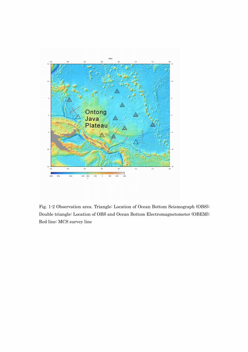
Fig. 1-2 Observation area. Triangle: Location of Ocean Bottom Seismograph (OBS); Double triangle: Location of OBS and Ocean Bottom Electromagnetometer (OBEM); Red line: MCS survey line
2. Background, purpose, and summary of the research cruise The Ontong Java Plateau (OJP) is the most voluminous Large Igneous Province on the oceanic region of
the Earth, which was emplaced at 120 million years ago by massive eruptions. The volcanic eruption gave
major environmental impacts, such as global climate change. However, the cause of the eruption remains
to be controversial due to a lack of the underground structure beneath the OJP. One of the main missions
of the project is to determine the underground structure beneath the OJP with an unprecedented accuracy.
For the purpose, we planned to deploy 23 ocean bottom seismographs (OBS) and 20 ocean bottom
electromagnetometers (OBEM) on the seafloor in and around the OJP during the Leg1 and Leg2 of the
MR14-06 cruise for determination of crust and upper mantle structure beneath the OJP. In the Leg1, we
deployed 11 OBS and 9 OBEM among all. The OBS and OBEM can continuously record an
electromagnetic field and ground motions due to natural earthquakes. The data are stored in the ocean
bottom instruments, which are planned to be recovered in 2016. The data will be used to determine
three-dimensional seismic and electrical conductivity structure, respectively. We also conducted
active-source high-resolution multichannel seismic reflection survey, multi-beam echo sounding survey,
sea-bottom reflectivity survey, gravity and magnetic surveys to study detailed shallow crustal and seafloor
structure, which should provide valuable information on the origin of the OJP and the evolution process.
A detailed survey was conducted near young seamounts and subduction zone to find exposed basements.
Another main mission of the R/V MIRAI MR14-06 cruise is to observe oceanographic and
atmospheric conditions in the tropical western Pacific to achieve a better understanding of air-sea
interaction over this region and its related climate change. To achieve this purpose, we will also perform
the following researches along the cruise track: Observation of aerosols and trace gases in the atmosphere,
which is important for global climate change, to analyze transport from the Asian continent to the ocean
environment along the winter monsoon; observation of precipitating clouds in ambient atmospheric and
oceanic situations to better estimate precipitation amount by utilizing ship-borne and satellite-borne
radars; acquisition of the validation data over sea for Greenhouse gases Observing SATellite (GOSAT)
using an automated compact instrument; installation of ARGO profiling floats to obtain vertical profiles
of sea temperatures and conductivity.

3. List of participants Principal Investigator: Dr. Daisuke Suetsugu
Director, Department of Deep Earth Structure and Dynamics Research
Japan Agency for Marine-Earth Science and Technology
2-15, Natsushima-cho, Yokosuka, 237-0061, Japan
Tel: +81-468-67-9755, FAX: +81-468-67-9315
e-mail: [email protected]
Table 3-1. Science party
Name Affiliation Appointment
Daisuke Suetsugu Department of Deep Earth Structure and Dynamics Research,
JAMSTEC
Director, scientist
Hiroko Sugioka Department of Deep Earth Structure and Dynamics Research,
JAMSTEC
Scientist
Noriko Tada Department of Deep Earth Structure and Dynamics Research,
JAMSTEC
Research scientist
Hiroshi, Ichihara Department of Deep Earth Structure and Dynamics Research,
JAMSTEC
Research scientist
Takehi Isse Earthquake Research Institute, the University of Tokyo Scientist
Shoka Shimizu Department of Deep Earth Structure and Dynamics Research,
JAMSTEC
Research student
Shungo Oshitani MWJ Technical Staff
Tatsuya Tanaka MWJ Technical Staff
Tomonori Watai MWJ Technical Staff
Masahiro Orui MWJ Technical Staff
Wataru Tokunaga GODI. Technical Staff
Miki Morioka GODI. Technical Staff
Koichi Inagaki GODI. Technical Staff
Makoto Ito NME. Technical Staff
Yuta Watarai NME. Technical Staff
Naoto Noguchi NME. Technical Staff
Ryo Miura NME. Technical Staff
Akie Suzuki NME. Technical Staff
Haruhiro Shibata NME. Technical Staff
JAMSTEC: Japan Agency for Marine-Earth Science and Technology GODI: Global Ocean Development Inc.

MWJ: Marine Work Japan Ltd.NME: Nippon Marine Enterprises Inc.
4. Deployment of ocean bottom seismograph (BBOBS)
(1) Personnel Daisuke Suetsugu (PI, JAMSTEC)Hiroko Sugioka (JAMSTEC)Takehi Isse (Earthquake Research Institute, the University of Tokyo)Wataru Tokunaga (Global Ocean Development, Ltd.)Miki Morioka (Global Ocean Development, Ltd.)Koichi Inagaki (Global Ocean Development, Ltd.)
(2) Objectives We deployed eleven OBSs to determine seismic structure of the crust and mantle beneath the
OJP region and its vicinity.
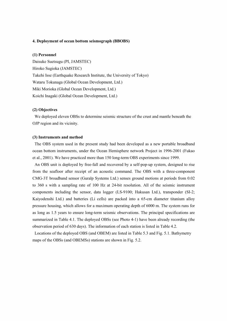
(3) Instruments and method The OBS system used in the present study had been developed as a new portable broadband
ocean bottom instruments, under the Ocean Hemisphere network Project in 1996-2001 (Fukao et al., 2001). We have practiced more than 150 long-term OBS experiments since 1999. An OBS unit is deployed by free-fall and recovered by a self-pop-up system, designed to rise
from the seafloor after receipt of an acoustic command. The OBS with a three-component CMG-3T broadband sensor (Guralp Systems Ltd.) senses ground motions at periods from 0.02 to 360 s with a sampling rate of 100 Hz at 24-bit resolution. All of the seismic instrument components including the sensor, data logger (LS-9100; Hakusan Ltd.), transponder (SI-2; Kaiyodenshi Ltd.) and batteries (Li cells) are packed into a 65-cm diameter titanium alloy pressure housing, which allows for a maximum operating depth of 6000 m. The system runs for as long as 1.5 years to ensure long-term seismic observations. The principal specifications are summarized in Table 4.1. The deployed OBSs (see Photo 4-1) have been already recording (the observation period of 630 days). The information of each station is listed in Table 4.2. Locations of the deployed OBS (and OBEM) are listed in Table 5.3 and Fig. 5.1. Bathymetry
maps of the OBSs (and OBEMSs) stations are shown in Fig. 5.2.
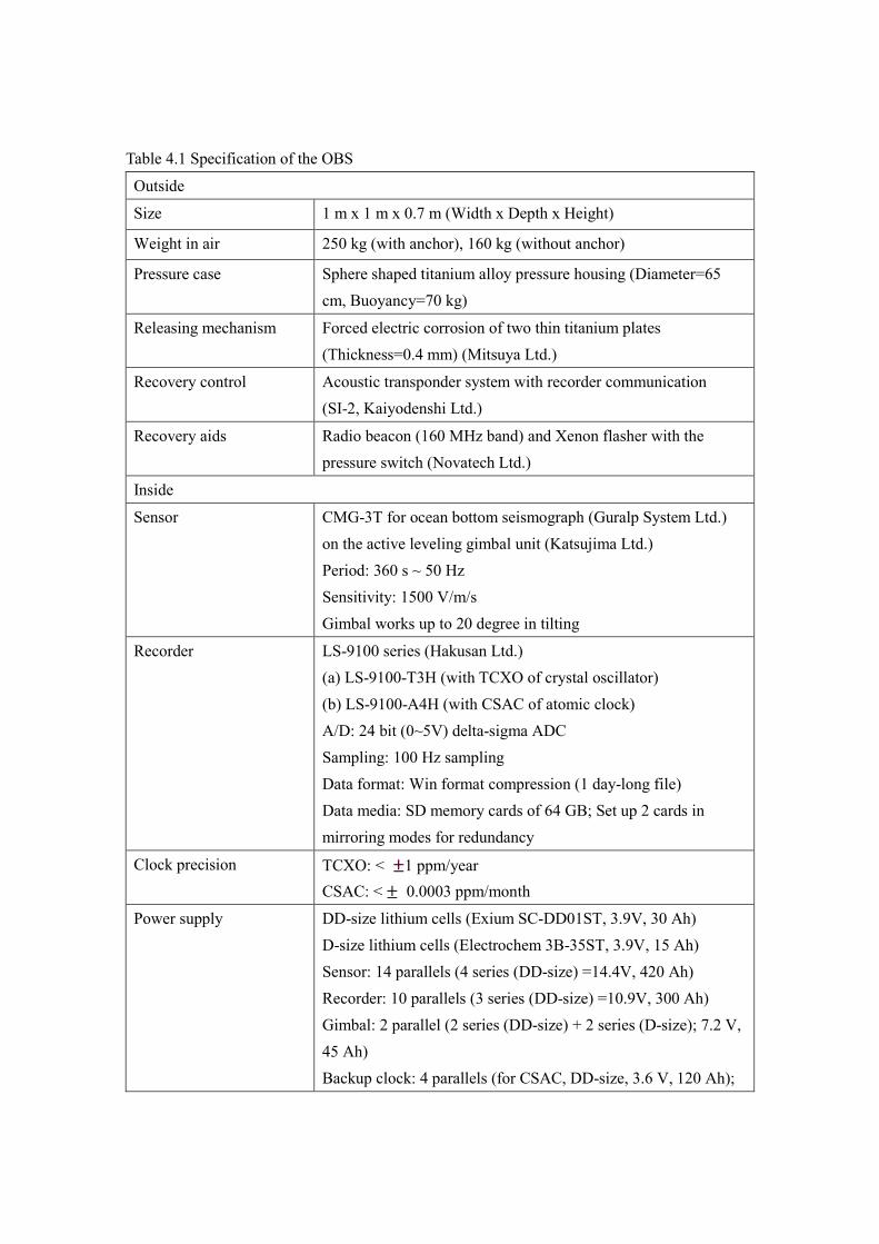
Table 4.1 Specification of the OBS
Outside
Size 1 m x 1 m x 0.7 m (Width x Depth x Height)
Weight in air 250 kg (with anchor), 160 kg (without anchor)
Pressure case Sphere shaped titanium alloy pressure housing (Diameter=65 cm, Buoyancy=70 kg)
Releasing mechanism Forced electric corrosion of two thin titanium plates (Thickness=0.4 mm) (Mitsuya Ltd.)
Recovery control Acoustic transponder system with recorder communication (SI-2, Kaiyodenshi Ltd.)
Recovery aids Radio beacon (160 MHz band) and Xenon flasher with the pressure switch (Novatech Ltd.)
Inside
Sensor CMG-3T for ocean bottom seismograph (Guralp System Ltd.) on the active leveling gimbal unit (Katsujima Ltd.) Period: 360 s ~ 50 Hz Sensitivity: 1500 V/m/s Gimbal works up to 20 degree in tilting
Recorder LS-9100 series (Hakusan Ltd.) (a) LS-9100-T3H (with TCXO of crystal oscillator) (b) LS-9100-A4H (with CSAC of atomic clock) A/D: 24 bit (0~5V) delta-sigma ADC Sampling: 100 Hz sampling Data format: Win format compression (1 day-long file) Data media: SD memory cards of 64 GB; Set up 2 cards in mirroring modes for redundancy
Clock precision TCXO: < 1 ppm/year CSAC: < ± 0.0003 ppm/month
Power supply DD-size lithium cells (Exium SC-DD01ST, 3.9V, 30 Ah) D-size lithium cells (Electrochem 3B-35ST, 3.9V, 15 Ah) Sensor: 14 parallels (4 series (DD-size) =14.4V, 420 Ah) Recorder: 10 parallels (3 series (DD-size) =10.9V, 300 Ah) Gimbal: 2 parallel (2 series (DD-size) + 2 series (D-size); 7.2 V, 45 Ah) Backup clock: 4 parallels (for CSAC, DD-size, 3.6 V, 120 Ah);
8 parallels (for TCXO, DD-size, 3.6 V, 240 Ah)
Power consumption Sensor: 360 mW Recorder: 140 mW (TCXO); 188 mW (CSAC) Gimbal: 14 mW Backup clock: 40 mW
Table 4.2 Information of deployed OBS
Site Clock
type
Tx
code
Radio freq.
[ MHz ]
S/N of
Seismograph
Gimbal
controller
Date of
deployment (LT)
Date ended of
recoding (UT)
O4 CSAC 813 159.200 T35594 SISEI312 2014/12/16 2016/09/06
O5 TCXO 539 159.300 T3H79 SISEI307’ 2014/12/09 2016/08/31
O15 TCXO 537 159.250 T3H55 SISEI308 2014/12/06 20146/08/27
O16 CSAC 810 159.350 T36786 SISEI308 2014/12/04 2016/08/25
O17 TCXO 504 159.150 T3D25 SISEI307’ 2014/11/28 2016/08/19
O18 TCXO 502 159.300 T3C08 SISEI307’ 2014/11/27 2016/08/18
O19 CSAC 812 159.300 T3D15 SISEI308 2014/11/24 2016/08/15
O20 CSAC 802 159.200 T3C05 SISEI308 2014/11/19 2016/08/10
O21 TCXO 515 159.300 T33854 SISEI310 2014/11/17 2016/08/09
O22 CSAC 816 159.150 T3M66 SISEI312 2014/11/16 2016/08/07
O23 TCXO 513 159.250 T3D14 SISEI308 2014/11/15 2016/08/06
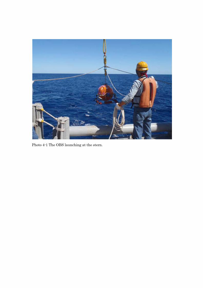
Photo 4-1 The OBS launching at the stern.
5. Deployment of ocean bottom electromagnetometers (OBEMs) (1) Personnel Daisuke Suetsugu (PI, JAMSTEC)Noriko Tada (JAMSTEC)Hiroshi Ichihara (JAMSTEC)Wataru Tokunaga (Global Ocean Development, Ltd.)Miki Morioka (Global Ocean Development, Ltd.)Koichi Inagaki (Global Ocean Development, Ltd.)
(2) Objectives We deployed nine OBEM to investigate electrical conductivity structure of the crust and
mantle beneath the OJP and its vicinity.
(3) Instruments and method The OBEM system can measure time variations of three components of magnetic field,
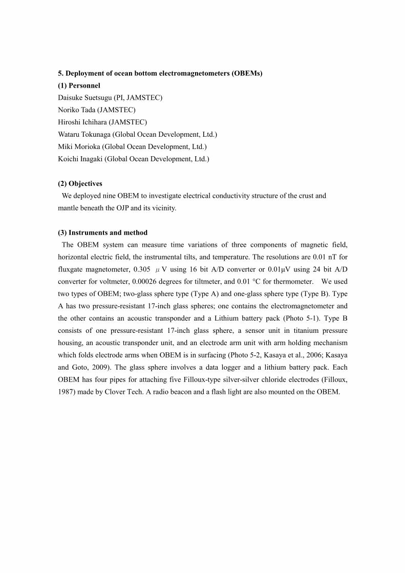
horizontal electric field, the instrumental tilts, and temperature. The resolutions are 0.01 nT for fluxgate magnetometer, 0.305 μV using 16 bit A/D converter or 0.01μV using 24 bit A/D converter for voltmeter, 0.00026 degrees for tiltmeter, and 0.01 °C for thermometer. We used two types of OBEM; two-glass sphere type (Type A) and one-glass sphere type (Type B). Type A has two pressure-resistant 17-inch glass spheres; one contains the electromagnetometer and the other contains an acoustic transponder and a Lithium battery pack (Photo 5-1). Type B consists of one pressure-resistant 17-inch glass sphere, a sensor unit in titanium pressure housing, an acoustic transponder unit, and an electrode arm unit with arm holding mechanism which folds electrode arms when OBEM is in surfacing (Photo 5-2, Kasaya et al., 2006; Kasaya and Goto, 2009). The glass sphere involves a data logger and a lithium battery pack. Each OBEM has four pipes for attaching five Filloux-type silver-silver chloride electrodes (Filloux, 1987) made by Clover Tech. A radio beacon and a flash light are also mounted on the OBEM.
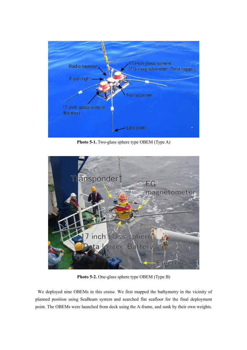
Photo 5-1. Two-glass sphere type OBEM (Type A)
Photo 5-2. One-glass sphere type OBEM (Type B)
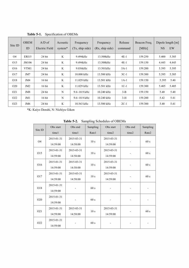
We deployed nine OBEMs in this cruise. We first mapped the bathymetry in the vicinity of planned position using SeaBeam system and searched flat seafloor for the final deployment point. The OBEMs were launched from deck using the A-frame, and sunk by their own weights.
The operations were quick and smooth. We confirmed that the OBEMs were successfully settled on the seafloor by measuring acoustic signals. Then, the settled positions were determined by measurements of the slant ranges at least three positions surrounding the launched point for each OBEM. The information that will be needed for the recovery and the data analysis are listed in Table 5-1. We used SSBL system equipped with R/V Mirai at the site O20 to measure slant ranges and determine the settled position The clocks of the OBEM were synchronized to UTC time before deployment by using a laptop PC using USB or RS232C communication. The laptop PC was synchronized by using GPS unit. Sampling schedules were also set before the OBEMs were deployed (Table 5-2).
Locations of the deployed OBEMs (and OBSs) are listed in Table 5.3 and Fig. 5.1. Bathymetry maps of the OBEMs (and OBSs) stations are shown in Fig. 5.2.
Ta b l e 5 -1. Specification of OBEMs
Site ID OBEM
ID
A/D of
Electric Field
Acoustic
system*
Frequency
(Tx, ship side)
Frequency
(Rx, ship side)
Release
command
Beacon Freq.
[MHz]
Dipole length [m]
NS EW
O4 ERI15 24 bit K 9.494kHz 13.500kHz 4E-1 159.250 5.400 5.385
O15 JM106 24 bit K 9.494kHz 13.500kHz 4E-1 159.150 4.445 4.445
O16 VTM1 24 bit K 9.036kHz 13.501kHz 5A-1 159.200 5.395 5.395
O17 JM7 24 bit K 10.000 kHz 13.500 kHz 3C-1 159.300 5.395 5.385
O18 JM4 16 bit K 11.029 kHz 13.501 kHz 1A-1 159.150 5.395 5.40
O20 JM2 16 bit K 11.029 kHz 13.501 kHz 1C-1 159.300 5.405 5.405
O21 JM8 24 bit N 9.6~10.9 kHz 10.240 kHz 3-B 159.150 5.40 5.40
O22 JM1 16 bit N 9.6~10.9 kHz 10.240 kHz 3-H 159.200 5.42 5.41
O23 JM6 24 bit K 10.563 kHz 13.500 kHz 2C-1 159.300 5.40 5.41
*K: Kaiyo Denshi, N: Nichiyu Giken
Ta b l e 5 -2. Sampling Schedules of OBEMs
Site ID Obs start
time1
Obs end
time1
Sampling
Rate1
Obs start
time2
Obs end
time2
Sampling
Rate2
O4 2015-01-31
14:59:00
2015-03-31
14:58:00 10 s
2015-03-31
14:59:00 - 60 s
O15 2015-01-31
14:59:00
2015-03-31
14:58:00 10 s
2015-03-31
14:59:00 - 60 s
O16 2015-01-31
14:59:00
2015-03-31
14:58:00 10 s
2015-03-31
14:59:00 - 60 s
O17 2015-01-31
14:59:00
2015-03-31
14:58:00 10 s
2015-03-31
14:59:00 - 60 s
O18 2015-01-31
14:59:00 - 60 s - - -
O20 2015-01-31
14:59:00 - 60 s - - -
O21 2015-01-31
14:59:00
2015-03-31
14:58:00 10 s
2015-03-31
14:59:00 - 60 s
O22 2015-01-31
14:59:00 - 60 s - - -

Table 5-3 Locations of deployed BBOBS and OBEM
Date of
deployment
(2014)
St.
code
BBOBS OBEM
latitude longitude depth latitude longitude depth
Nov. 15 O23 06-57.265N 164-29.796E 5117m 06-57.178N 164-29.766E 5116m
Nov. 16 O22 02-52.264N 166-01.581E 4309m 02-52.166N 166-01.683E 4308m
Nov. 17 O21 00-01.552N 170-00.278E 4458m 00-01.405N 170-00.169E 4459m
Nov. 19 O20 02-56.745S 174-59.442E 5077m 02-56.737S 174-59.424E 5078m
Nov. 23 O19 08-00.729S 170-03.190E 4860m ― ― ―
Nov. 27 O18 03-53.272S 166-42.490E 3441m 03-53.275S 166-42.609E 3440m
Nov. 28 O17 00-59.112S 164-00.514E 4435m 00-59.193S 164-00.402E 4434m
Dec. 4 O16 06-25.040S 163-25.009E 3558m 06-25.080S 163-25.047E 3559m
Dec. 6 O15 05-57.891S 160-02.448E 1813m 05-57.881S 160-02.399E 1813m
Dec. 9 O5 00-36.928S 153-00.113E 4337m ― ― ―
Dec. 16 O4 04-27.000N 150-22.978E 3987m 04-26.961N 150-23.058E 3986m
Fig. 5-1 Deployed OBS and OBEM stations. Triangles: OBS stations; Double triangles; OBS and OBEM stations

Fig. 5.2a Bathymetry at the O23 station.
Fig. 5.2b Bathymetry at the O22 station.
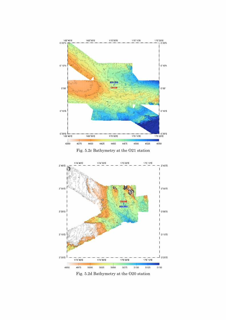
Fig. 5.2c Bathymetry at the O21 station
Fig. 5.2d Bathymetry at the O20 station
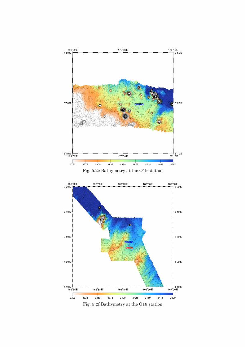
Fig. 5.2e Bathymetry at the O19 station
Fig. 5-2f Bathymetry at the O18 station
Fig. 5.2g Bathymetry at the O17 station
Fig. 5.2h Bathymetry at the O16 station
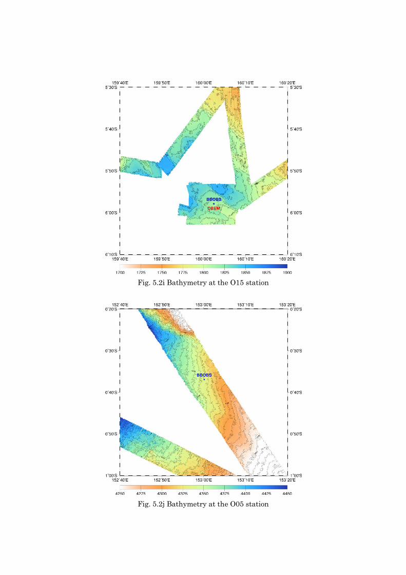
Fig. 5.2i Bathymetry at the O15 station
Fig. 5.2j Bathymetry at the O05 station
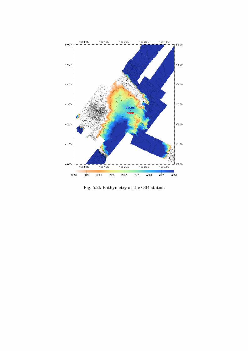
Fig. 5.2k Bathymetry at the O04 station
6. High resolution multichannel seismic reflection survey for crustal structure of the Ontong Java Plateau Daisuke Suetsugu (PI, JAMSTEC)Masao Nakanishi (Chiba Universsity, not onboard)Makoto Ito (NME.)Yuta Watari (NME.)Naoto Noguchi (NME.)Ryo Miura (NME.)Akie Suzuki (NME.)Haruhiro Shibata (NME.)
6-1. Purpose We performed high resolution multichannel seismic reflection (MCS) survey to determine shallow crustal structure in the OJP area, since it should bears a key to understand an evolution process of the OJP. Depending on the evolution process, seismic signatures such as fault and rift could remain in the crust of the OJP, which should be imaged by the MCS survey.
6-2. Instruments The MCS system is composed of a cluster air-gun array and a streamer cable with a tail buoy at the end. The MCS system was towed with a speed of 3-4 knots. Specification of the instrument is shown in Table 6-1. We also towed a Cesium magnetometer of to obtain a magnetic signature along the survey lines.
Table 6-1. Specification of the MCS system
Source: cluster airgun array
Air volume: 380 inch3 of total volume (40 inch3×2 + 150 inch3×2)
Air pressure: 2000psi
Shot interval: 37.5m
Airgun depth: 3m
Streamer cable
L1 Channel: 168 Cable length: 1341m Cable depth:
4m
Hydrophone
interval: 6.25m
L2, L4, L5,
L6, L8
Channel: 160 Cable length:
1290~1200m
Cable depth:
4m
Hydrophone
interval: 6.25m
L7 Channel: 144 Cable length: 1150m Cable depth:
4m
Hydrophone
interval: 6.25m
Note: L3 line was cancelled due to failure of the streamer cable.
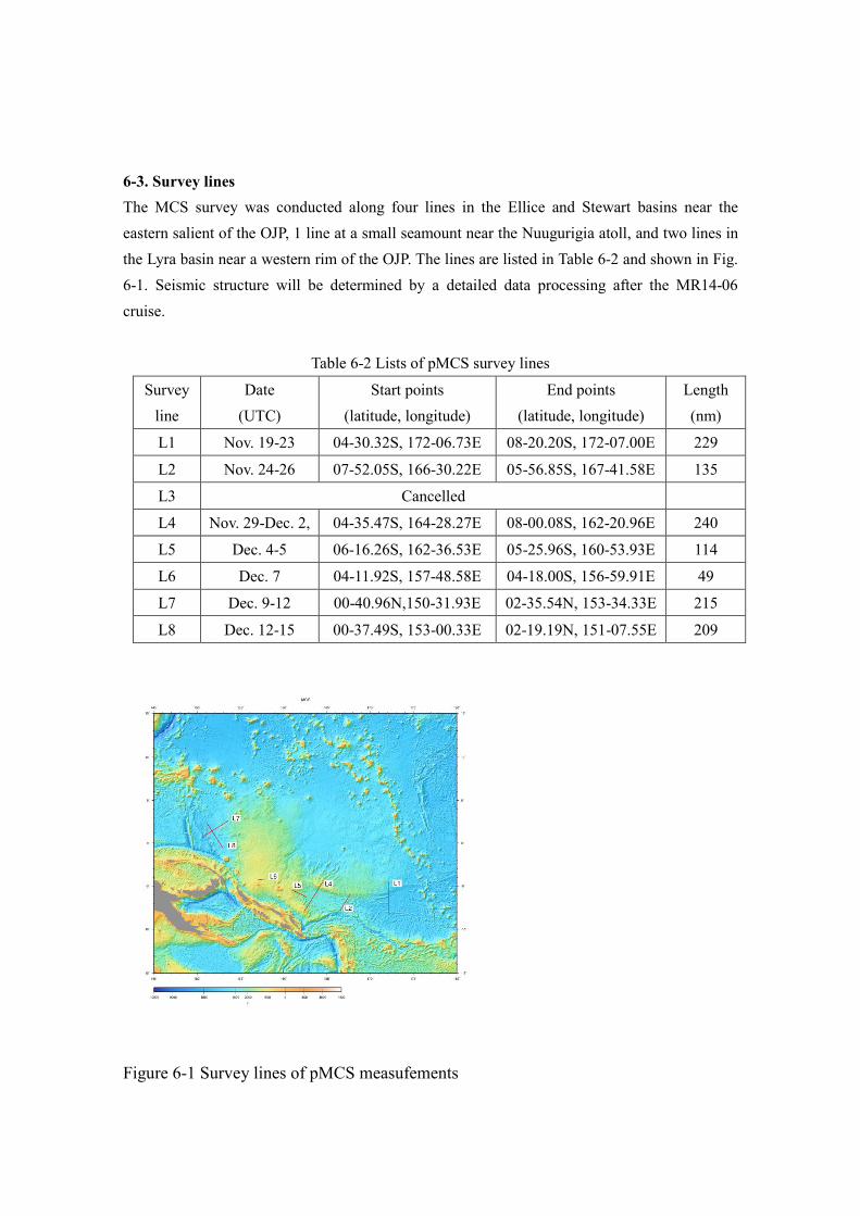
6-3. Survey lines The MCS survey was conducted along four lines in the Ellice and Stewart basins near the eastern salient of the OJP, 1 line at a small seamount near the Nuugurigia atoll, and two lines in the Lyra basin near a western rim of the OJP. The lines are listed in Table 6-2 and shown in Fig. 6-1. Seismic structure will be determined by a detailed data processing after the MR14-06 cruise.
Table 6-2 Lists of pMCS survey lines
Survey line
Date (UTC)
Start points (latitude, longitude)
End points (latitude, longitude)
Length (nm)
L1 Nov. 19-23 04-30.32S, 172-06.73E 08-20.20S, 172-07.00E 229
L2 Nov. 24-26 07-52.05S, 166-30.22E 05-56.85S, 167-41.58E 135
L3 Cancelled
L4 Nov. 29-Dec. 2, 04-35.47S, 164-28.27E 08-00.08S, 162-20.96E 240
L5 Dec. 4-5 06-16.26S, 162-36.53E 05-25.96S, 160-53.93E 114
L6 Dec. 7 04-11.92S, 157-48.58E 04-18.00S, 156-59.91E 49
L7 Dec. 9-12 00-40.96N,150-31.93E 02-35.54N, 153-34.33E 215
L8 Dec. 12-15 00-37.49S, 153-00.33E 02-19.19N, 151-07.55E 209
Figure 6-1 Survey lines of pMCS measufements
7. Search for basement rocks of the Ontong Java Plateau
(1)Personnel
Takeshi Hanyu (PI, JAMSTEC, not onboard)
Shoka Shimizu (JAMSTEC)
Wataru Tokunaga (GODI)
Miki Morioka (GODI)
Koichi Inagaki (GODI)
(2) Objectives Since the Ontong Java Plateau (OJP) sits largely under the ocean, rock sampling has been
thus far restricted. A surface of the OJP is largely covered with thick sediments, which also make it difficult to sample rocks. We need to search potential sites where basement rocks are exposed for successful sampling that will provide a key to elucidate an origin of the OJP. During the MR14-06 cruise, we have searched for feasible sites of the rock sampling with underway geophysical survey. We plan to sample rocks with a dredge in 2016 at the sites where rocks are likely to be exposed at the seafloor.
(3) Observation sites and methods We have performed multi narrow beam echo sounding system, sub-bottom profiler, towing
cesium magnetometer, ship-board three-component magnetometer, and gravity meter at four sites: Off the east coast of the Malaita island; flanks of three submarine volcanoes on the OJP, whose the top is an atoll (the Ontong Java atoll, the Cartrete atoll, and the Nuguria atoll). The Malaita sites are a convergence zone of the OJP and the North Solomon trench. It is selected for the survey, since a previous study of an MCS survey (Phinney et al., 2004, Tectonophysics, 389, 221-246) suggests that there is places where a sediment is very thin or nil, which may be a suitable site for sampling igneous rocks with a dredge.
The three submarine volcanoes are selected because we found that a flank of another submarine volcanoes (Nuugurigia), similar to the three volcanoes, has a small cones where igneous rocks are exposed. It leads us to an idea that the three atolls have volcanic cones on their flanks, which are potential sites of exposed rocks.
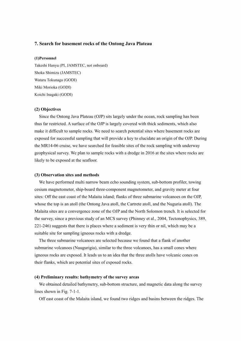
(4) Preliminary results: bathymetry of the survey areas We obtained detailed bathymetry, sub-bottom structure, and magnetic data along the survey
lines shown in Fig. 7-1-1. Off east coast of the Malaita island, we found two ridges and basins between the ridges. The
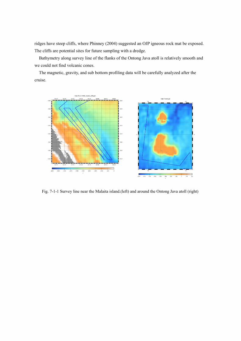
ridges have steep cliffs, where Phinney (2004) suggested an OJP igneous rock mat be exposed. The cliffs are potential sites for future sampling with a dredge.
Bathymetry along survey line of the flanks of the Ontong Java atoll is relatively smooth and we could not find volcanic cones.
The magnetic, gravity, and sub bottom profiling data will be carefully analyzed after the cruise.
Fig. 7-1-1 Survey line near the Malaita island.(left) and around the Ontong Java atoll (right)
8. General observations 8.1. Meteorological measurements 8.1.1 Surface Meteorological Observations
(1) Personnel Daisuke Suetsugu (JAMSTEC) : Principal Investigator
Wataru Tokunaga (Global Ocean Development Inc. GODI)
Koichi Inagaki (GODI)
Miki Morioka (GODI)
Masanori Murakami (MIRAI Crew)
(2) Objectives Surface meteorological parameters are observed as a basic dataset of the meteorology.
These parameters provide the temporal variation of the meteorological condition surrounding the ship.
(3) Methods Surface meteorological parameters were observed during the MR14-06 Leg1 cruise from
4th November 2014 to 17th December 2014, without territorial waters on Independent State of Papua New Guinea and Federated States of Micronesia. In this cruise, we used two systems for the observation.
i. MIRAI Surface Meteorological observation (SMet) system Instruments of SMet system are listed in Table 8.1.1-1 and measured parameters are
listed in Table 8.1.1-2. Data were collected and processed by KOAC-7800 weather data processor made by Koshin-Denki, Japan. The data set consists of 6-second averaged data.
ii. Shipboard Oceanographic and Atmospheric Radiation (SOAR) measurement system SOAR system designed by BNL (Brookhaven National Laboratory, USA) consists of
major five parts.
a) Portable Radiation Package (PRP) designed by BNL – short and long wave downward radiation.
b) Analog meteorological data sampling with CR1000 logger manufactured by Campbell Inc. Canada – wind, pressure, and rainfall (by a capacitive rain gauge) measurement.
c) Digital meteorological data sampling from individual sensors - air temperature, relative humidity and rainfall (by ORG (optical rain gauge)) measurement.
d) Photosynthetically Available Radiation (PAR) sensor manufactured by Biospherical Instruments Inc. (USA) - PAR measurement.
e) Scientific Computer System (SCS) developed by NOAA (National Oceanic and Atmospheric Administration, USA) – centralized data acquisition and logging of all data sets.
SCS recorded PRP data every 6 seconds, CR1000 data every 10 seconds, air temperature and relative humidity data every 2 seconds and ORG data every 5 seconds. SCS composed Event data (JamMet) from these data and ship’s navigation data. Instruments and their locations are listed in Table 8.1.1-3 and measured parameters are listed in Table 8.1.1-4.
For the quality control as post processing, we checked the following sensors, before and after the cruise.
i. Young Rain gauge (SMet and SOAR) Inspect of the linearity of output value from the rain gauge sensor to change Input value by adding fixed quantity of test water.
ii. Barometer (SMet and SOAR) Comparison with the portable barometer value, PTB220, VAISALA
iii. Thermometer (air temperature and relative humidity) ( SMet and SOAR ) Comparison with the portable thermometer value, HMP41/45, VAISALA
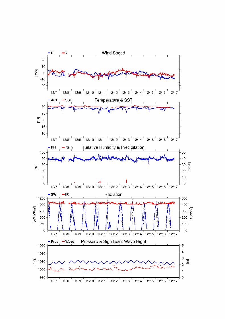
(4) Preliminary results Fig. 8.1.1-1 shows the time series of the following parameters;
Wind (SMet)Air temperature (SMet)Relative humidity (SMet)Precipitation (SOAR, rain gauge)Short/long wave radiation (SOAR)Pressure (SMet)Sea surface temperature (SMet)Significant wave height (SMet)
(5) Data archives These meteorological data will be submitted to the Data Management Group (DMG) of
JAMSTEC just after the cruise.
(6) Remarks (Times in UTC) i) The following periods, Sea surface temperature of SMet data was available.
08:57 07 Nov. 2014 - 05:30 17 Dec. 2014
ii) The following time, increasing of SMet capacitive rain gauge data were invalid due to transmitting for VHF or MF/HF radio. 07:24 07 Nov. 2014 04:42 12 Nov. 2014
iii) The following period, downwelling radiometer (short wave) was invalid.26 Nov. 2014 - 17 Dec. 2014
iv) SOAR true wind direction and speed were invalid due to fail relative direction of anemometer during this cruise.
v) The following period, PAR data was invalid due to maintenance. 13:31 09 Nov. 2014 - 13:36 09 Nov. 2014
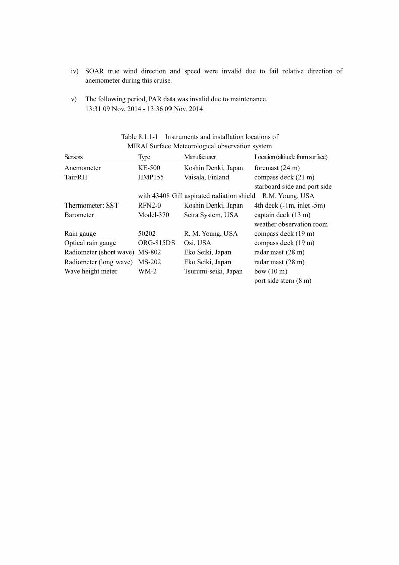
Table 8.1.1-1 Instruments and installation locations of MIRAI Surface Meteorological observation system
Sensors Type Manufacturer Location (altitude from surface) Anemometer KE-500 Koshin Denki, Japan foremast (24 m) Tair/RH HMP155 Vaisala, Finland compass deck (21 m)
starboard side and port side with 43408 Gill aspirated radiation shield R.M. Young, USA
Thermometer: SST RFN2-0 Koshin Denki, Japan 4th deck (-1m, inlet -5m) Barometer Model-370 Setra System, USA captain deck (13 m)
weather observation room Rain gauge 50202 R. M. Young, USA compass deck (19 m) Optical rain gauge ORG-815DS Osi, USA compass deck (19 m) Radiometer (short wave) MS-802 Eko Seiki, Japan radar mast (28 m) Radiometer (long wave) MS-202 Eko Seiki, Japan radar mast (28 m) Wave height meter WM-2 Tsurumi-seiki, Japan bow (10 m)
port side stern (8 m)
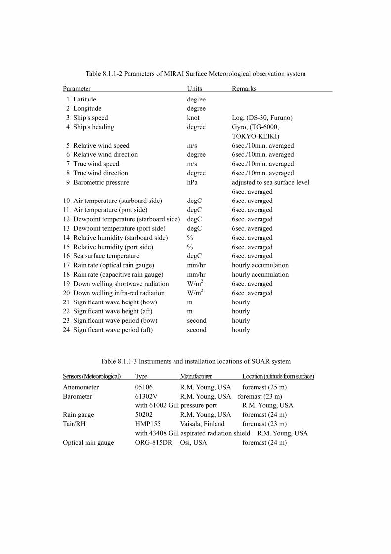
Table 8.1.1-2 Parameters of MIRAI Surface Meteorological observation system
Parameter Units Remarks 1 Latitude degree 2 Longitude degree 3 Ship’s speed knot Log, (DS-30, Furuno) 4 Ship’s heading degree Gyro, (TG-6000,
TOKYO-KEIKI) 5 Relative wind speed m/s 6sec./10min. averaged 6 Relative wind direction degree 6sec./10min. averaged 7 True wind speed m/s 6sec./10min. averaged 8 True wind direction degree 6sec./10min. averaged 9 Barometric pressure hPa adjusted to sea surface level
6sec. averaged 10 Air temperature (starboard side) degC 6sec. averaged 11 Air temperature (port side) degC 6sec. averaged 12 Dewpoint temperature (starboard side) degC 6sec. averaged 13 Dewpoint temperature (port side) degC 6sec. averaged 14 Relative humidity (starboard side) % 6sec. averaged 15 Relative humidity (port side) % 6sec. averaged 16 Sea surface temperature degC 6sec. averaged 17 Rain rate (optical rain gauge) mm/hr hourly accumulation 18 Rain rate (capacitive rain gauge) 19 Down welling shortwave radiation
mm/hr W/m2
hourly accumulation 6sec. averaged
20 Down welling infra-red radiation W/m2 6sec. averaged 21 Significant wave height (bow) m hourly 22 Significant wave height (aft) m hourly 23 Significant wave period (bow) second hourly 24 Significant wave period (aft) second hourly
Table 8.1.1-3 Instruments and installation locations of SOAR system
Sensors (Meteorological) Type Manufacturer Location (altitude from surface) Anemometer 05106 R.M. Young, USA foremast (25 m) Barometer 61302V R.M. Young, USA foremast (23 m)
with 61002 Gill pressure port R.M. Young, USA Rain gauge 50202 R.M. Young, USA foremast (24 m) Tair/RH HMP155 Vaisala, Finland foremast (23 m)
with 43408 Gill aspirated radiation shield R.M. Young, USA Optical rain gauge ORG-815DR Osi, USA foremast (24 m)
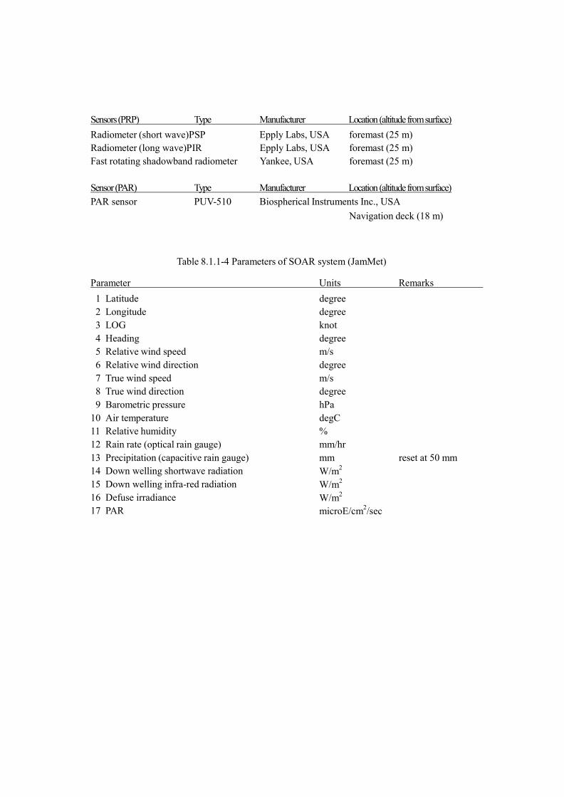
Sensors (PRP) Type Manufacturer Location (altitude from surface)
Radiometer (short wave)PSP Epply Labs, USA foremast (25 m) Radiometer (long wave)PIR Epply Labs, USA foremast (25 m) Fast rotating shadowband radiometer Yankee, USA foremast (25 m)
Sensor (PAR) Type Manufacturer Location (altitude from surface) PAR sensor PUV-510 Biospherical Instruments Inc., USA
Navigation deck (18 m)
Table 8.1.1-4 Parameters of SOAR system (JamMet)
Parameter Units Remarks
1 Latitude degree 2 Longitude degree 3 LOG knot 4 Heading degree 5 Relative wind speed m/s 6 Relative wind direction degree 7 True wind speed m/s 8 True wind direction degree 9 Barometric pressure hPa
10 Air temperature degC 11 Relative humidity % 12 Rain rate (optical rain gauge) mm/hr 13 Precipitation (capacitive rain gauge) mm reset at 50 mm 14 Down welling shortwave radiation W/m2 15 Down welling infra-red radiation W/m2 16 Defuse irradiance W/m2 17 PAR microE/cm2/sec
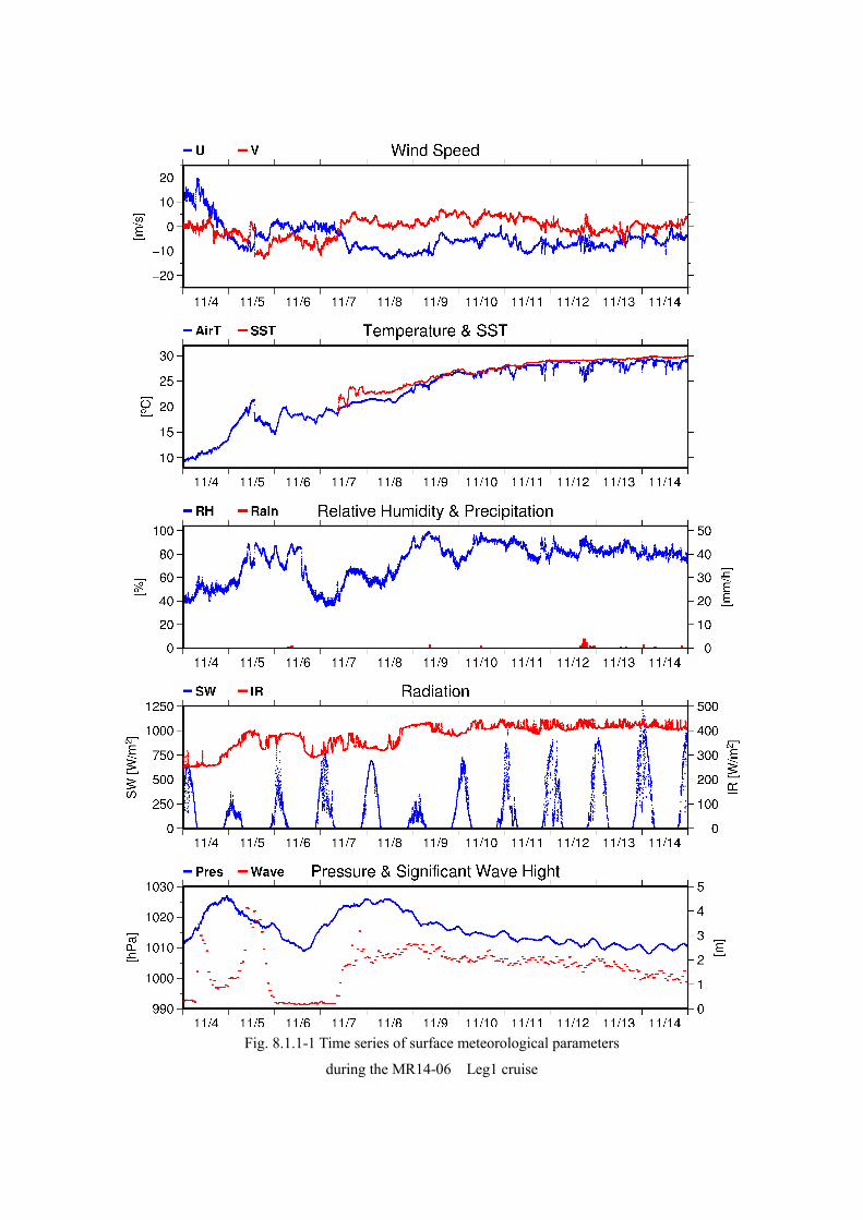
Fig. 8.1.1-1 Time series of surface meteorological parameters
during the MR14-06 Leg1 cruise
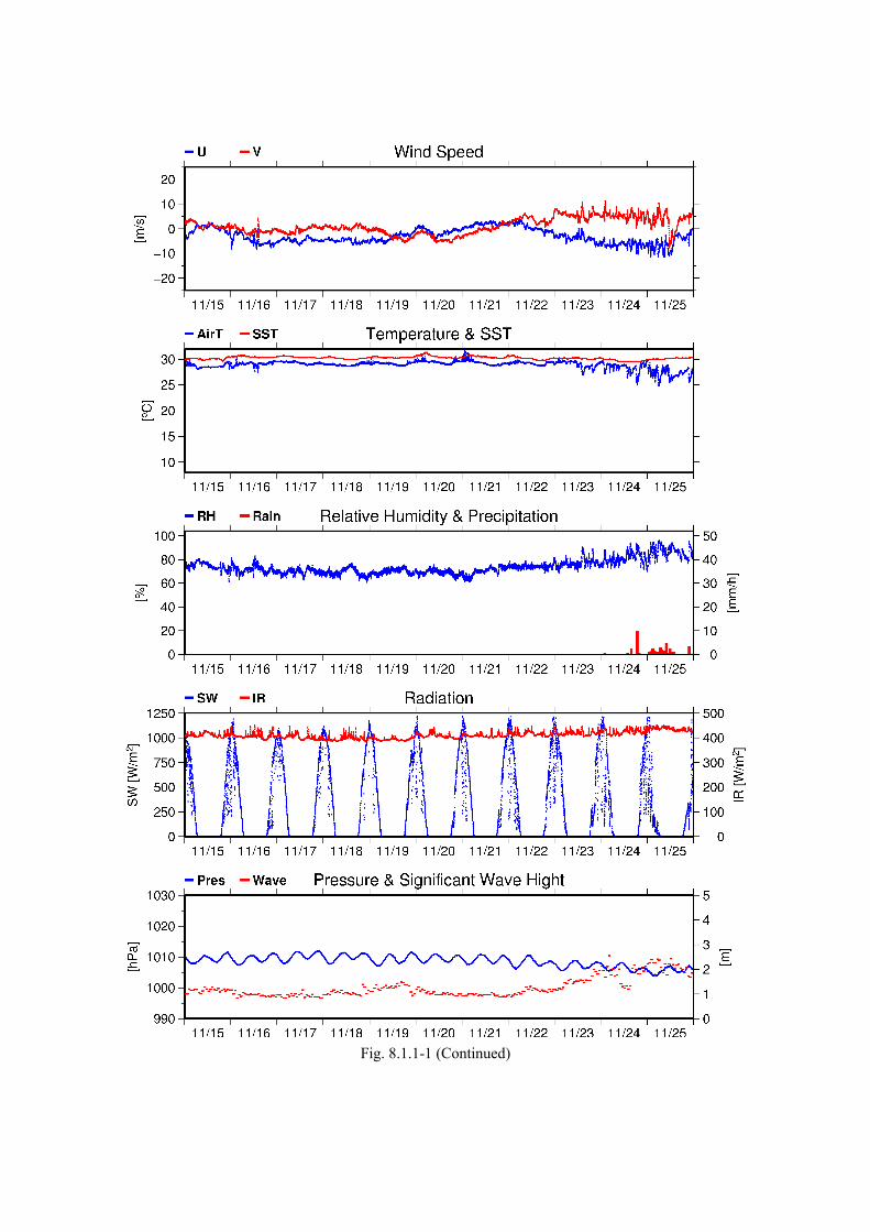
Fig. 8.1.1-1 (Continued)
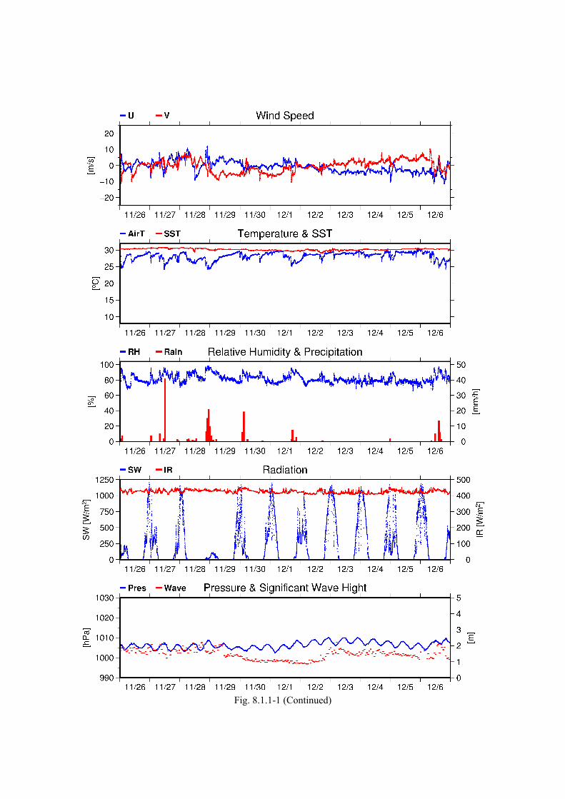
Fig. 8.1.1-1 (Continued)
---------------------------------------------------------------------------------------------------------------------------
---------------------------------------------------------------------------------------------------------------------------
Fig. 8.1.1-1 (Continued)
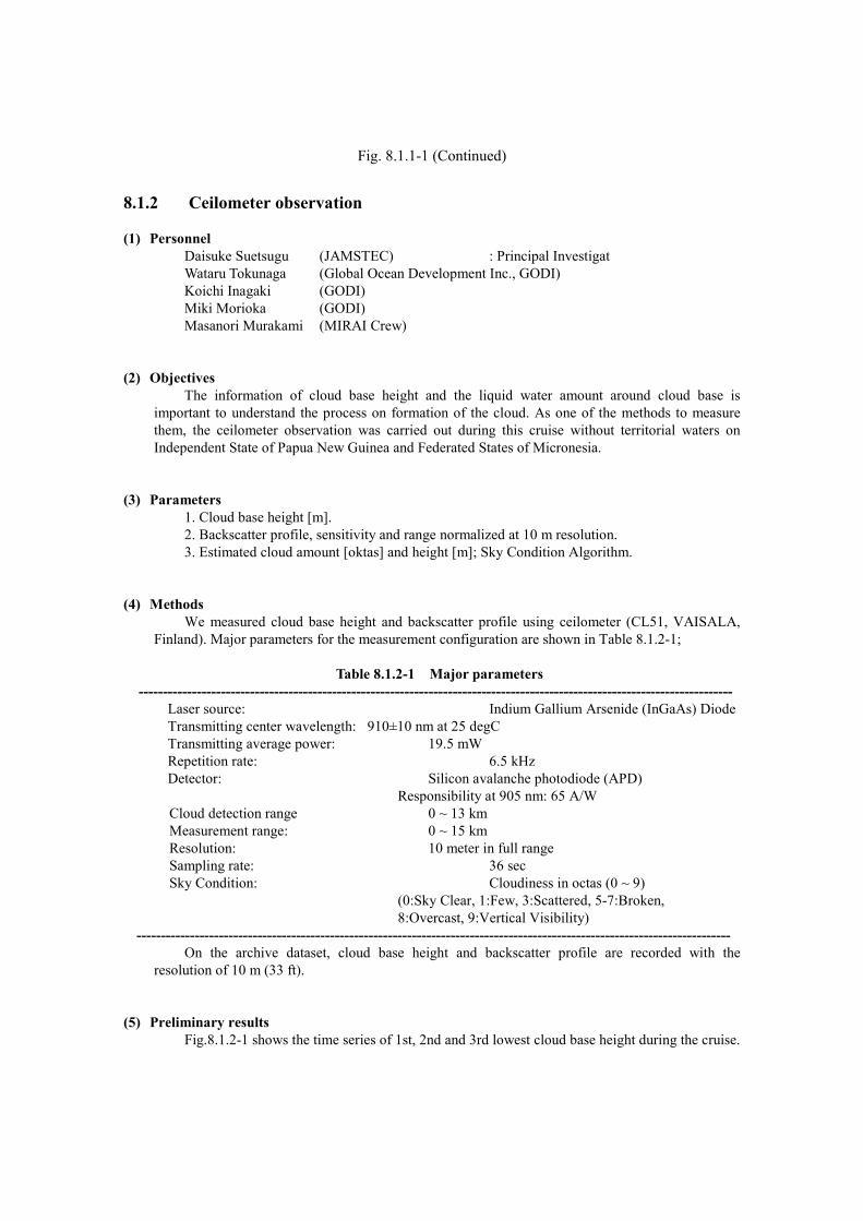
8.1.2 Ceilometer observation
(1) Personnel Daisuke Suetsugu (JAMSTEC) : Principal InvestigatWataru Tokunaga (Global Ocean Development Inc., GODI)Koichi Inagaki (GODI)Miki Morioka (GODI)Masanori Murakami (MIRAI Crew)
(2) Objectives The information of cloud base height and the liquid water amount around cloud base is
important to understand the process on formation of the cloud. As one of the methods to measure them, the ceilometer observation was carried out during this cruise without territorial waters on Independent State of Papua New Guinea and Federated States of Micronesia.
(3) Parameters 1. Cloud base height [m]. 2. Backscatter profile, sensitivity and range normalized at 10 m resolution. 3. Estimated cloud amount [oktas] and height [m]; Sky Condition Algorithm.
(4) Methods We measured cloud base height and backscatter profile using ceilometer (CL51, VAISALA,
Finland). Major parameters for the measurement configuration are shown in Table 8.1.2-1;
Table 8.1.2-1 Major parameters
Laser source: Indium Gallium Arsenide (InGaAs) Diode Transmitting center wavelength: 910±10 nm at 25 degC Transmitting average power: 19.5 mW Repetition rate: 6.5 kHz Detector: Silicon avalanche photodiode (APD)
Responsibility at 905 nm: 65 A/WCloud detection range 0 ~ 13 kmMeasurement range: 0 ~ 15 kmResolution: 10 meter in full rangeSampling rate: 36 secSky Condition: Cloudiness in octas (0 ~ 9)
(0:Sky Clear, 1:Few, 3:Scattered, 5-7:Broken, 8:Overcast, 9:Vertical Visibility)
On the archive dataset, cloud base height and backscatter profile are recorded with the resolution of 10 m (33 ft).
(5) Preliminary results Fig.8.1.2-1 shows the time series of 1st, 2nd and 3rd lowest cloud base height during the cruise.

(6) Data archives The raw data obtained during this cruise will be submitted to the Data Management Group
(DMG) of JAMSTEC.
(7) Remarks (Times in UTC) i) The following time, the window was cleaned.
04:41UTC 04 Nov. 2014 22:07UTC 09 Nov. 2014 19:22UTC 16 Nov. 2014 23:00UTC 24 Nov. 2014 21:27UTC 02 Dec. 2014 19:54UTC 09 Dec. 2014 20:36UTC 15 Dec. 2014
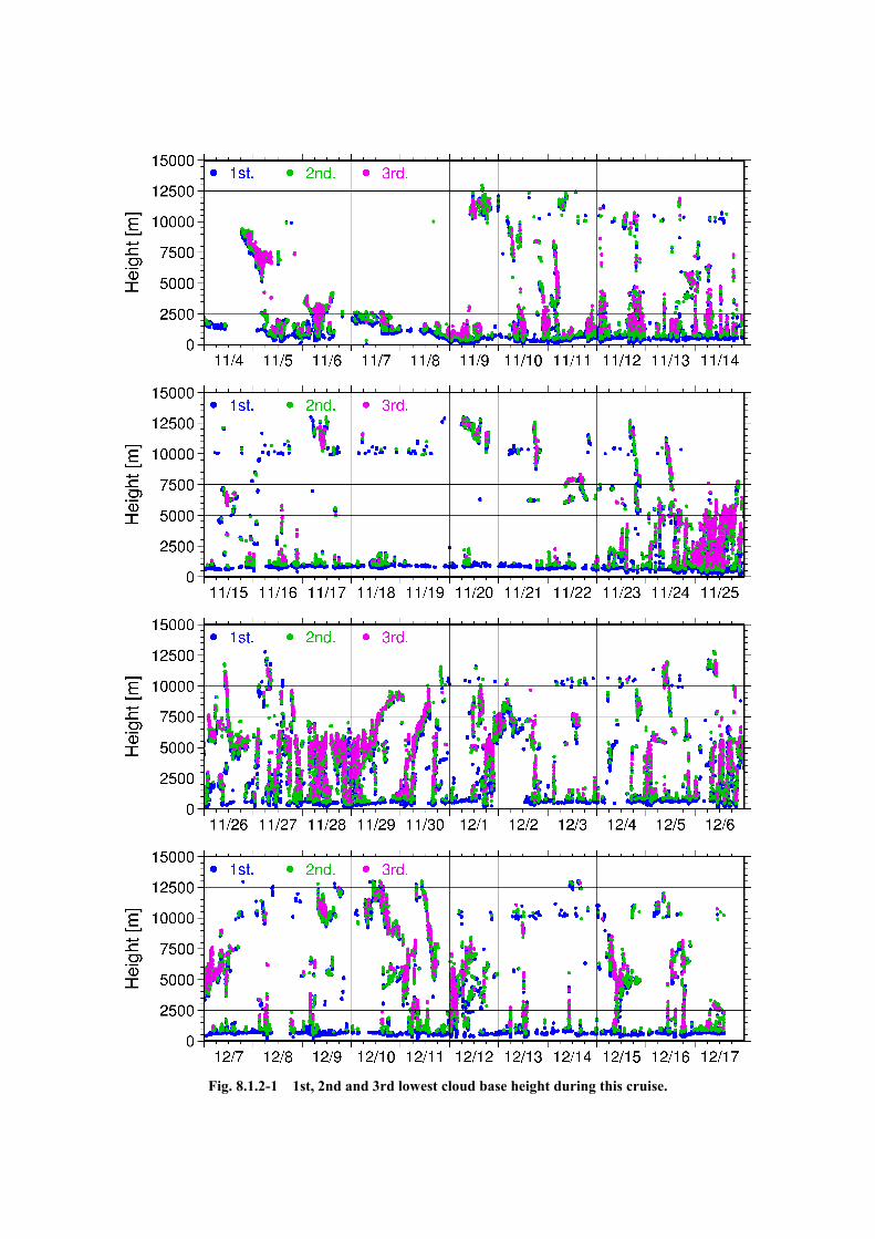
Fig. 8.1.2-1 1st, 2nd and 3rd lowest cloud base height during this cruise.
8.1.3. Aerosol optical characteristics measured by ship-borne sky radiometer
(1) Personnel
Kazuma Aoki (PI, University of Toyama, not onboard)
Tadahiro Hayasaka (Tohoku University, not onboard)
(2) Objective
Objective of this observation is to study distribution and optical characteristics of marine aerosols
by using a ship-borne sky radiometer (POM-01 MKII: PREDE Co. Ltd., Japan). Furthermore,
collections of the data for calibration and validation to the remote sensing data were performed
simultaneously.
(3) Parameters
- Aerosol optical thickness at five wavelengths (400, 500, 675, 870 and 1020 nm)
- Ångström exponent
- Single scattering albedo at five wavelengths
- Size distribution of volume (0.01 µm – 20 µm)
- # GPS provides the position with longitude and latitude and heading direction of the vessel,
and azimuth and elevation angle of the sun. Horizon sensor provides rolling and pitching
angles.
(4) Instruments and Methods
The sky radiometer measures the direct solar irradiance and the solar aureole radiance distribution
with seven interference filters (0.34, 0.4, 0.5, 0.675, 0.87, 0.94, and 1.02 µm). Analysis of these
data was performed by SKYRAD.pack version 4.2 developed by Nakajima et al. 1996.
(5) Data archives
Aerosol optical data are to be archived at University of Toyama (K.Aoki, SKYNET/SKY:
http://skyrad.sci.u-toyama.ac.jp/) after the quality check and will be submitted to JAMSTEC.
8.1.4 Tropospheric gas and particle observation in the marine atmosphere
(1) Personnel Yugo Kanaya (DEGCR/JAMSTEC, not onboard) Fumikazu Taketani (DEGCR/JAMSTEC, not onboard) Takuma Miyakawa (DEGCR/JAMSTEC, not onboard) Hisahiro Takashima (DEGCR/JAMSTEC, not onboard) Yuichi Komazaki (DEGCR/JAMSTEC, not onboard) Maki Noguchi (RCGC/JAMSTEC, not onboard) Operation was supported by GODI.
(2) Objective • To investigate roles of aerosols in the marine atmosphere in relation to climate change • To investigate processes of biogeochemical cycles between the atmosphere and the ocean.
(3) Parameter • Black carbon(BC) particles • Composition of ambient particles • Aerosol optical depth (AOD) and Aerosol extinction coefficient (AEC) • Surface ozone(O3), and carbon monoxide(CO) mixing ratios
(4) Description of instruments deployed(4-1) Online aerosol observations of black carbon (BC)
BC particles were measured by an instrument based on laser-induced incandescence (SP2, Droplet Measurement Technologies). For SP2, ambient air was commonly sampled from the flying bridge by a 3-m-long conductive tube through the Diffusion Dryer(model TSI) to dry up the particles, and then introduced to each instrument. The laser-induced incandescence technique based on intracavity Nd:YVO4 laser operating at 1064 nm were used for detection of single particles of BC. (4-2) Ambient air sampling by high-volume air sampler
Ambient aerosol particles were collected along cruise track using a high-volume air sampler (HV-525PM, SIBATA) located on the flying bridge operated at a flow rate of 500 L min-1. To avoid collecting particles emitted from the funnel of the own vessel, the sampling period was controlled automatically by using a “wind-direction selection system”. Coarse and fine particles separated at the diameter of 2.5 μm were collected on quartz filters. The filter samples obtained during the cruise are subject to chemical analysis of aerosol composition, including water-soluble ions and trace metals. (4-3) MAX-DOAS
Multi-Axis Differential Optical Absorption Spectroscopy (MAX-DOAS), a passive remote sensing technique measuring spectra of scattered visible and ultraviolet (UV) solar radiation, was used for atmospheric aerosol and gas profile measurements. Our MAX-DOAS instrument consists of two main parts: an outdoor telescope unit and an indoor spectrometer
(Acton SP-2358 with Princeton Instruments PIXIS-400B), connected to each other by a 14-m bundle optical fiber cable. The line of sight was in the directions of the portside of the vessel and the measurements were made at several elevation angles of 1.5, 3, 5, 10, 20, 30, 90 degrees using a movable prism, which repeated the same sequence of elevation angles every ~15-min.For the selected spectra recorded with elevation angles with good accuracy, DOAS spectral fitting was performed to quantify the slant column density (SCD) of NO2 (and other gases) and O4 (O2-O2, collision complex of oxygen) for each elevation angle. Then, the O4
SCDs were converted to the aerosol optical depth (AOD) and the vertical profile of aerosol extinction coefficient (AEC) using an optimal estimation inversion method with a radiative transfer model. Using derived aerosol information, retrievals of the tropospheric vertical column/profile of NO2 and other gases were made. (4-4) CO and O3
Ambient air was continuously sampled on the compass deck and drawn through ~20-m-long Teflon tubes connected to a gas filter correlation CO analyzer (Model 48C, Thermo Fisher Scientific) and a UV photometric ozone analyzer (Model 49C, Thermo Fisher Scientific), located in the Research Information Center. The data will be used for characterizing air mass origins.
(5) Observation log The shipboard measurements and sampling were conducted in the open sea
(6) Preliminary results N/A (All the data analysis is to be conducted.)
(7) Data archive The data files will be submitted to JAMSTEC Data Management Group (DMG), after
the full analysis is completed, which will be <2 years after the end of the cruise.
8.1.5 Disdrometers
(1) Personnel Masaki Katsumata (PI, JAMSTEC, not onboard)
(2) Objectives The disdrometer can continuously obtain size distribution of raindrops. The objective of this observation is (a) to reveal microphysical characteristics of the rainfall, depends on the type, temporal stage, etc. of the precipitating clouds, (b) to retrieve the coefficient to convert radar reflectivity to the rainfall amount, and (c) to validate the algorithms and the product of the satellite-borne precipitation radars; TRMM/PR and GPM/DPR.
Parameters Number and size of precipitating particles
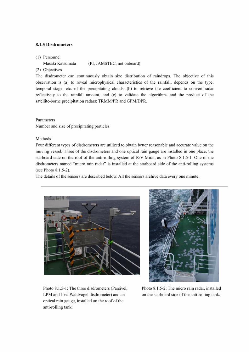
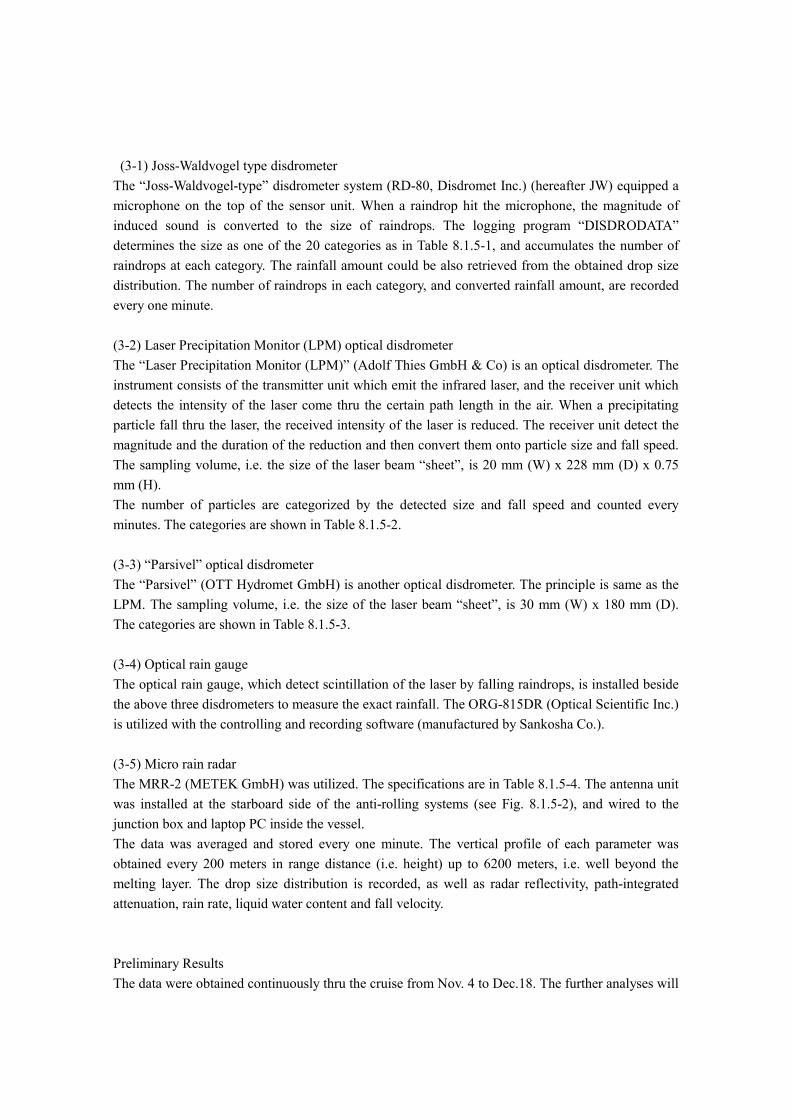
Methods Four different types of disdrometers are utilized to obtain better reasonable and accurate value on the moving vessel. Three of the disdrometers and one optical rain gauge are installed in one place, the starboard side on the roof of the anti-rolling system of R/V Mirai, as in Photo 8.1.5-1. One of the disdrometers named “micro rain radar” is installed at the starboard side of the anti-rolling systems (see Photo 8.1.5-2). The details of the sensors are described below. All the sensors archive data every one minute.
Photo 8.1.5-1: The three disdrometers (Parsivel, LPM and Joss-Waldvogel disdrometer) and an optical rain gauge, installed on the roof of the anti-rolling tank.
Photo 8.1.5-2: The micro rain radar, installed on the starboard side of the anti-rolling tank.
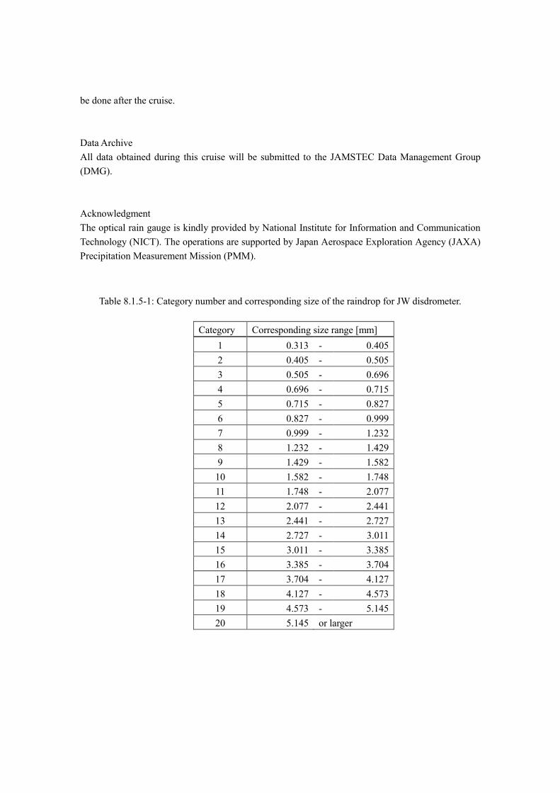
(3-1) Joss-Waldvogel type disdrometerThe “Joss-Waldvogel-type” disdrometer system (RD-80, Disdromet Inc.) (hereafter JW) equipped amicrophone on the top of the sensor unit. When a raindrop hit the microphone, the magnitude ofinduced sound is converted to the size of raindrops. The logging program “DISDRODATA”determines the size as one of the 20 categories as in Table 8.1.5-1, and accumulates the number ofraindrops at each category. The rainfall amount could be also retrieved from the obtained drop sizedistribution. The number of raindrops in each category, and converted rainfall amount, are recordedevery one minute.
(3-2) Laser Precipitation Monitor (LPM) optical disdrometerThe “Laser Precipitation Monitor (LPM)” (Adolf Thies GmbH & Co) is an optical disdrometer. Theinstrument consists of the transmitter unit which emit the infrared laser, and the receiver unit which detects the intensity of the laser come thru the certain path length in the air. When a precipitating particle fall thru the laser, the received intensity of the laser is reduced. The receiver unit detect themagnitude and the duration of the reduction and then convert them onto particle size and fall speed.The sampling volume, i.e. the size of the laser beam “sheet”, is 20 mm (W) x 228 mm (D) x 0.75mm (H).The number of particles are categorized by the detected size and fall speed and counted everyminutes. The categories are shown in Table 8.1.5-2.
(3-3) “Parsivel” optical disdrometerThe “Parsivel” (OTT Hydromet GmbH) is another optical disdrometer. The principle is same as theLPM. The sampling volume, i.e. the size of the laser beam “sheet”, is 30 mm (W) x 180 mm (D).The categories are shown in Table 8.1.5-3.
(3-4) Optical rain gaugeThe optical rain gauge, which detect scintillation of the laser by falling raindrops, is installed besidethe above three disdrometers to measure the exact rainfall. The ORG-815DR (Optical Scientific Inc.)is utilized with the controlling and recording software (manufactured by Sankosha Co.).
(3-5) Micro rain radarThe MRR-2 (METEK GmbH) was utilized. The specifications are in Table 8.1.5-4. The antenna unitwas installed at the starboard side of the anti-rolling systems (see Fig. 8.1.5-2), and wired to thejunction box and laptop PC inside the vessel.The data was averaged and stored every one minute. The vertical profile of each parameter wasobtained every 200 meters in range distance (i.e. height) up to 6200 meters, i.e. well beyond themelting layer. The drop size distribution is recorded, as well as radar reflectivity, path-integratedattenuation, rain rate, liquid water content and fall velocity.
Preliminary ResultsThe data were obtained continuously thru the cruise from Nov. 4 to Dec.18. The further analyses will
be done after the cruise.
Data ArchiveAll data obtained during this cruise will be submitted to the JAMSTEC Data Management Group(DMG).
AcknowledgmentThe optical rain gauge is kindly provided by National Institute for Information and Communication Technology (NICT). The operations are supported by Japan Aerospace Exploration Agency (JAXA)Precipitation Measurement Mission (PMM).
Table 8.1.5-1: Category number and corresponding size of the raindrop for JW disdrometer.
Category Corresponding size range [mm] 1 0.313 - 0.405 2 0.405 - 0.505 3 0.505 - 0.696 4 0.696 - 0.715 5 0.715 - 0.827 6 0.827 - 0.999 7 0.999 - 1.232 8 1.232 - 1.429 9 1.429 - 1.582 10 1.582 - 1.748 11 1.748 - 2.077 12 2.077 - 2.441 13 2.441 - 2.727 14 2.727 - 3.011 15 3.011 - 3.385 16 3.385 - 3.704 17 3.704 - 4.127 18 4.127 - 4.573 19 4.573 - 5.145 20 5.145 or larger
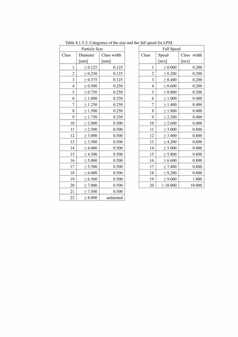
Table 8.1.5-2: Categories of the size and the fall speed for LPM. Particle Size
Class Diameter [mm]
Class width [mm]
1 ≥ 0.125 0.125 2 ≥ 0.250 0.125 3 ≥ 0.375 0.125 4 ≥ 0.500 0.250 5 ≥ 0.750 0.250 6 ≥ 1.000 0.250 7 ≥ 1.250 0.250 8 ≥ 1.500 0.250 9 ≥ 1.750 0.250
10 ≥ 2.000 0.500 11 ≥ 2.500 0.500 12 ≥ 3.000 0.500 13 ≥ 3.500 0.500 14 ≥ 4.000 0.500 15 ≥ 4.500 0.500 16 ≥ 5.000 0.500 17 ≥ 5.500 0.500 18 ≥ 6.000 0.500 19 ≥ 6.500 0.500 20 ≥ 7.000 0.500 21 ≥ 7.500 0.500 22 ≥ 8.000 unlimited
Fall Speed Class Speed
[m/s] Class width [m/s]
1 ≥ 0.000 0.200 2 ≥ 0.200 0.200 3 ≥ 0.400 0.200 4 ≥ 0.600 0.200 5 ≥ 0.800 0.200 6 ≥ 1.000 0.400 7 ≥ 1.400 0.400 8 ≥ 1.800 0.400 9 ≥ 2.200 0.400
10 ≥ 2.600 0.400 11 ≥ 3.000 0.800 12 ≥ 3.400 0.800 13 ≥ 4.200 0.800 14 ≥ 5.000 0.800 15 ≥ 5.800 0.800 16 ≥ 6.600 0.800 17 ≥ 7.400 0.800 18 ≥ 8.200 0.800 19 ≥ 9.000 1.000 20 ≥ 10.000 10.000
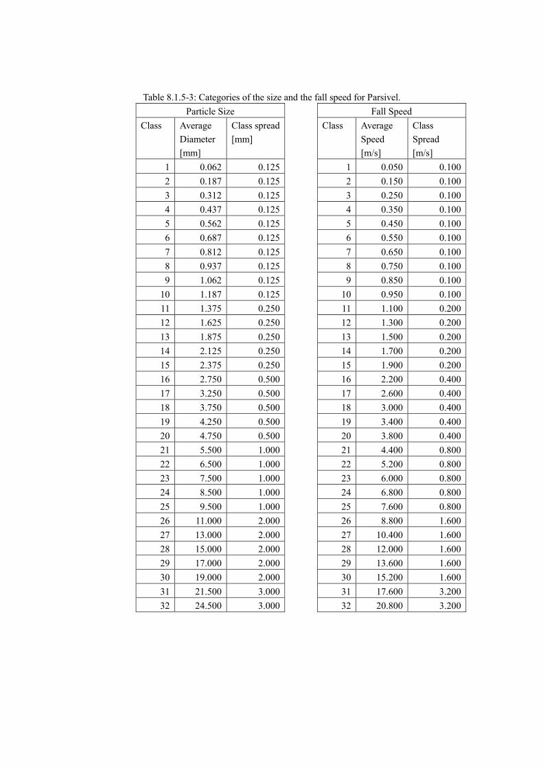
Table 8.1.5-3: Categories of the size and the fall speed for Parsivel. Particle Size
Class Average Diameter [mm]
Class spread [mm]
1 0.062 0.125 2 0.187 0.125 3 0.312 0.125 4 0.437 0.125 5 0.562 0.125 6 0.687 0.125 7 0.812 0.125 8 0.937 0.125 9 1.062 0.125
10 1.187 0.125 11 1.375 0.250 12 1.625 0.250 13 1.875 0.250 14 2.125 0.250 15 2.375 0.250 16 2.750 0.500 17 3.250 0.500 18 3.750 0.500 19 4.250 0.500 20 4.750 0.500 21 5.500 1.000 22 6.500 1.000 23 7.500 1.000 24 8.500 1.000 25 9.500 1.000 26 11.000 2.000 27 13.000 2.000 28 15.000 2.000 29 17.000 2.000 30 19.000 2.000 31 21.500 3.000 32 24.500 3.000
Fall Speed Class Average
Speed [m/s]
Class Spread [m/s]
1 0.050 0.100 2 0.150 0.100 3 0.250 0.100 4 0.350 0.100 5 0.450 0.100 6 0.550 0.100 7 0.650 0.100 8 0.750 0.100 9 0.850 0.100
10 0.950 0.100 11 1.100 0.200 12 1.300 0.200 13 1.500 0.200 14 1.700 0.200 15 1.900 0.200 16 2.200 0.400 17 2.600 0.400 18 3.000 0.400 19 3.400 0.400 20 3.800 0.400 21 4.400 0.800 22 5.200 0.800 23 6.000 0.800 24 6.800 0.800 25 7.600 0.800 26 8.800 1.600 27 10.400 1.600 28 12.000 1.600 29 13.600 1.600 30 15.200 1.600 31 17.600 3.200 32 20.800 3.200

Table 8.1.5-4: Specifications of the MRR-2. Transmitter power 50 mW Operating mode FM-CW Frequency 24.230 GHz
(modulation 1.5 to 15 MHz) 3dB beam width 1.5 degrees Spurious emission < -80 dBm / MHz Antenna Diameter 600 mm Gain 40.1 dBi
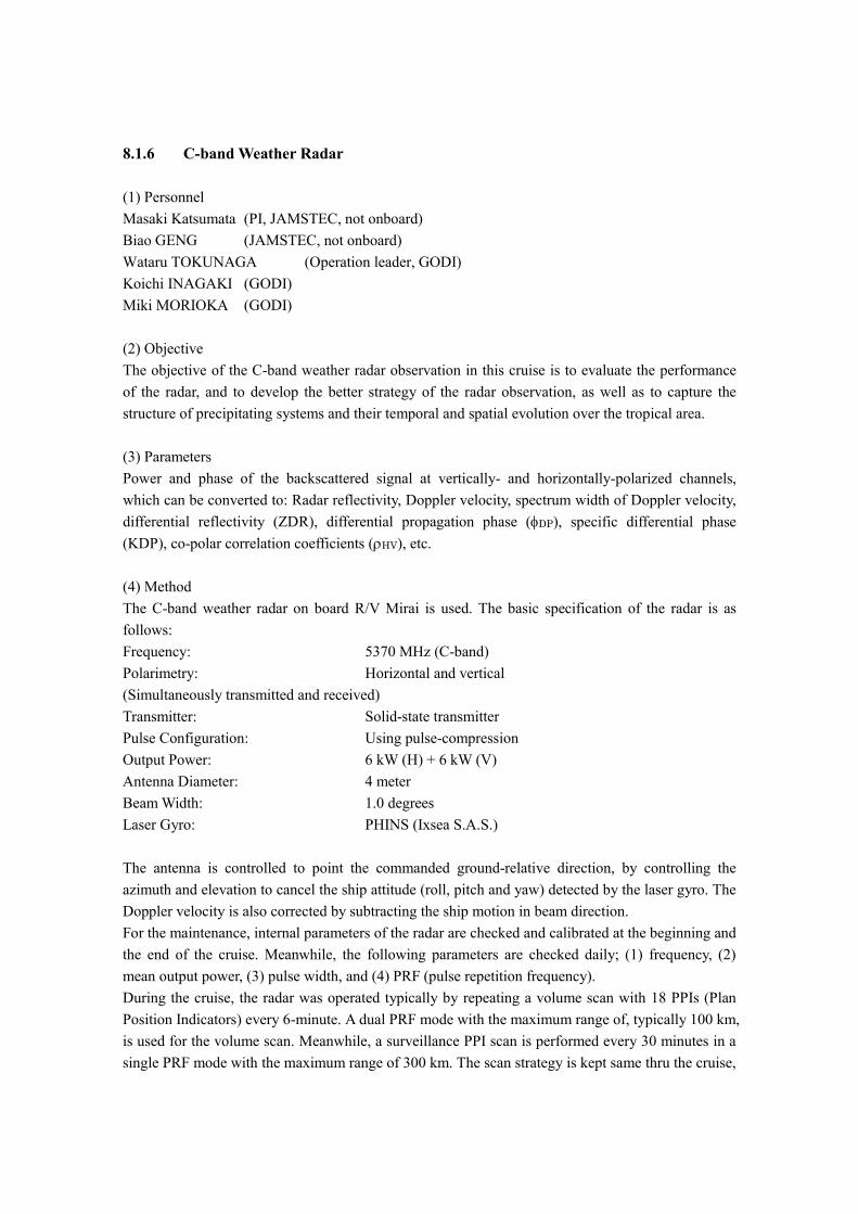
8.1.6 C-band Weather Radar
(1) PersonnelMasaki Katsumata (PI, JAMSTEC, not onboard)Biao GENG (JAMSTEC, not onboard)Wataru TOKUNAGA (Operation leader, GODI)Koichi INAGAKI (GODI)Miki MORIOKA (GODI)
(2) ObjectiveThe objective of the C-band weather radar observation in this cruise is to evaluate the performanceof the radar, and to develop the better strategy of the radar observation, as well as to capture thestructure of precipitating systems and their temporal and spatial evolution over the tropical area.
(3) ParametersPower and phase of the backscattered signal at vertically- and horizontally-polarized channels,which can be converted to: Radar reflectivity, Doppler velocity, spectrum width of Doppler velocity, differential reflectivity (ZDR), differential propagation phase (φDP), specific differential phase(KDP), co-polar correlation coefficients (ρHV), etc.
(4) MethodThe C-band weather radar on board R/V Mirai is used. The basic specification of the radar is as follows:Frequency: 5370 MHz (C-band)Polarimetry: Horizontal and vertical(Simultaneously transmitted and received)Transmitter: Solid-state transmitter Pulse Configuration: Using pulse-compression Output Power: 6 kW (H) + 6 kW (V) Antenna Diameter: 4 meter Beam Width: 1.0 degrees Laser Gyro: PHINS (Ixsea S.A.S.)
The antenna is controlled to point the commanded ground-relative direction, by controlling theazimuth and elevation to cancel the ship attitude (roll, pitch and yaw) detected by the laser gyro. TheDoppler velocity is also corrected by subtracting the ship motion in beam direction.For the maintenance, internal parameters of the radar are checked and calibrated at the beginning andthe end of the cruise. Meanwhile, the following parameters are checked daily; (1) frequency, (2)mean output power, (3) pulse width, and (4) PRF (pulse repetition frequency).During the cruise, the radar was operated typically by repeating a volume scan with 18 PPIs (PlanPosition Indicators) every 6-minute. A dual PRF mode with the maximum range of, typically 100 km,is used for the volume scan. Meanwhile, a surveillance PPI scan is performed every 30 minutes in asingle PRF mode with the maximum range of 300 km. The scan strategy is kept same thru the cruise,
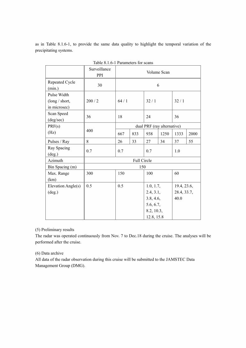
as in Table 8.1.6-1, to provide the same data quality to highlight the temporal variation of the precipitating systems.
Table 8.1.6-1 Parameters for scans Surveillance
PPI Volume Scan
Repeated Cycle (min.)
30 6
Pulse Width (long / short, in microsec)
200 / 2 64 / 1 32 / 1 32 / 1
Scan Speed (deg/sec)
36 18 24 36
PRF(s) (Hz) 400
dual PRF (ray alternative)
667 833 938 1250 1333 2000
Pulses / Ray 8 26 33 27 34 37 55 Ray Spacing (deg.)
0.7 0.7 0.7 1.0
Azimuth Full Circle Bin Spacing (m) 150 Max. Range (km)
300 150 100 60
Elevation Angle(s) (deg.)
0.5 0.5 1.0, 1.7, 2.4, 3.1, 3.8, 4.6, 5.6, 6.7, 8.2, 10.3, 12.8, 15.8
19.4, 23.6, 28.4, 33.7, 40.0
(5) Preliminary results The radar was operated continuously from Nov. 7 to Dec.18 during the cruise. The analyses will be performed after the cruise.
(6) Data archive All data of the radar observation during this cruise will be submitted to the JAMSTEC Data Management Group (DMG).
8.1.7 Shipboard CO2 observations over the tropical Indo-Pacific Ocean for a simple estimation of the carbon flux between the ocean and the atmosphere from GOSAT data
(1) Personnel Shuji Kawakami (PI, EORC/JAXA) Kei Shiomi (EORC/JAXA)
(2) Objectives Greenhouse gases Observing SATellite (GOSAT) was launched on 23 January 2009 in
order to observe the global distributions of atmospheric greenhouse gas concentrations: column-averaged dry-air mole fractions of carbon dioxide (CO2) and methane (CH4). A network of ground-based high-resolution Fourier transform spectrometers provides essential validation data for GOSAT. Vertical CO2 profiles obtained during ascents and descents of commercial airliners equipped with the in-situ CO2 measuring instrument are also used for the GOSAT validation. Because such validation data are obtained mainly over land, there are very few data available for the validation of the over-sea GOSAT products. The objectives of our research are to acquire the validation data over the Indian Ocean and the tropical Pacific Ocean using an automated compact instrument, to compare the acquired data with the over-sea GOSAT products, and to develop a simple estimation of the carbon flux between the ocean and the atmosphere from GOSAT data.
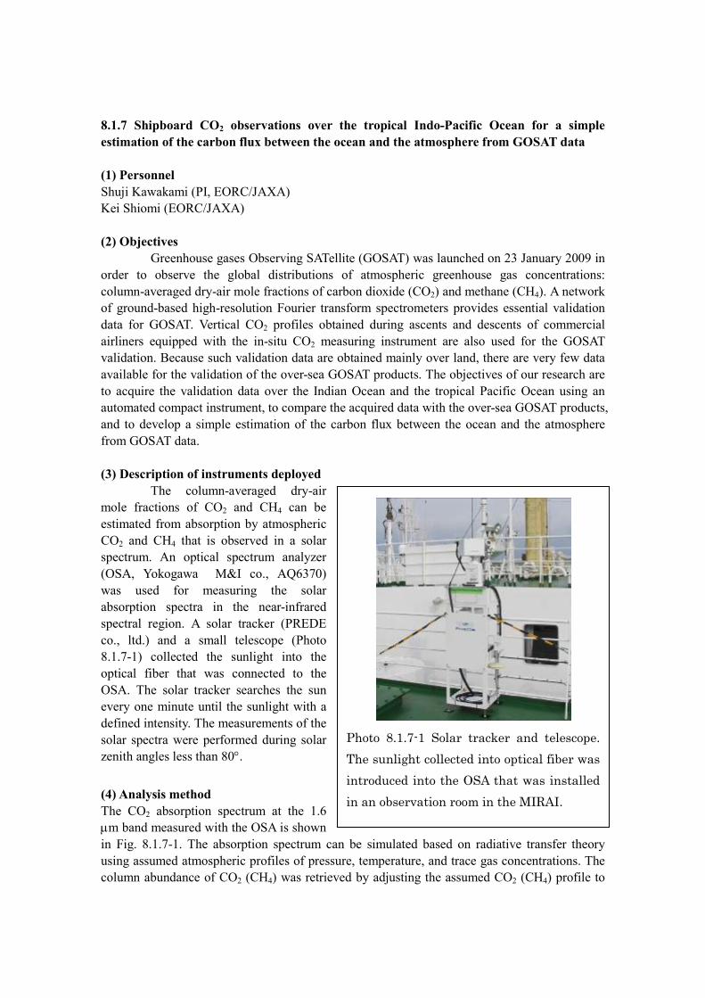
(3) Description of instruments deployed The column-averaged dry-air
mole fractions of CO2 and CH4 can be estimated from absorption by atmospheric CO2 and CH4 that is observed in a solar spectrum. An optical spectrum analyzer (OSA, Yokogawa M&I co., AQ6370) was used for measuring the solar absorption spectra in the near-infrared spectral region. A solar tracker (PREDE co., ltd.) and a small telescope (Photo 8.1.7-1) collected the sunlight into the optical fiber that was connected to the OSA. The solar tracker searches the sun every one minute until the sunlight with a defined intensity. The measurements of the solar spectra were performed during solar zenith angles less than 80°.
(4) Analysis method The CO2 absorption spectrum at the 1.6 µm band measured with the OSA is shown in Fig. 8.1.7-1. The absorption spectrum can be simulated based on radiative transfer theory using assumed atmospheric profiles of pressure, temperature, and trace gas concentrations. The column abundance of CO2 (CH4) was retrieved by adjusting the assumed CO2 (CH4) profile to
Photo 8.1.7-1 Solar tracker and telescope. The sunlight collected into optical fiber was introduced into the OSA that was installed in an observation room in the MIRAI.
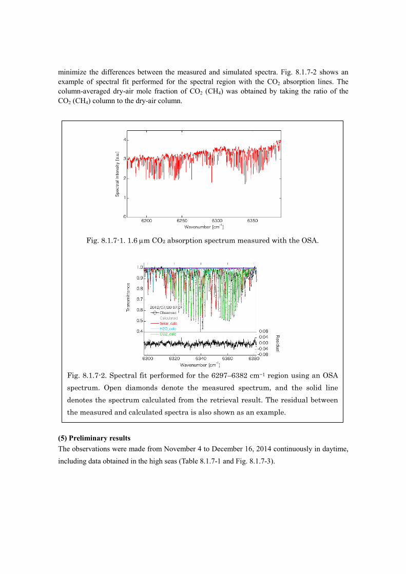
minimize the differences between the measured and simulated spectra. Fig. 8.1.7-2 shows an example of spectral fit performed for the spectral region with the CO2 absorption lines. The column-averaged dry-air mole fraction of CO2 (CH4) was obtained by taking the ratio of the CO2 (CH4) column to the dry-air column.
Fig. 8.1.7-1. 1.6 µm CO2 absorption spectrum measured with the OSA.
Fig. 8.1.7-2. Spectral fit performed for the 6297–6382 cm−1 region using an OSA spectrum. Open diamonds denote the measured spectrum, and the solid line denotes the spectrum calculated from the retrieval result. The residual between the measured and calculated spectra is also shown as an example.
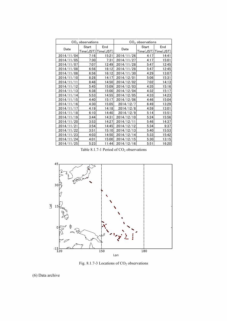
(5) Preliminary results The observations were made from November 4 to December 16, 2014 continuously in daytime, including data obtained in the high seas (Table 8.1.7-1 and Fig. 8.1.7-3).
CO2 observations CO2 observations
Date Start
Time(JST) End
Time(JST) Date
Start Time(JST)
End Time(JST)
2014/11/04 7:16 15:21 2014/11/26 4:17 14:41 2014/11/05 7:30 7:31 2014/11/27 4:17 15:01 2014/11/07 7:07 12:49 2014/11/28 5:47 12:45 2014/11/08 6:56 16:12 2014/11/28 5:47 12:45 2014/11/08 6:56 16:12 2014/11/30 4:29 13:07 2014/11/10 8:28 14:17 2014/12/01 5:06 15:31 2014/11/11 8:48 14:50 2014/12/02 7:02 14:13 2014/11/12 5:45 15:09 2014/12/03 4:35 15:16 2014/11/13 6:38 15:00 2014/12/04 4:32 15:17 2014/11/14 5:53 14:55 2014/12/05 4:33 14:23 2014/11/15 4:40 15:17 2014/12/06 4:46 15:04 2014/11/16 4:30 15:05 2014/12/7 6:49 13:29 2014/11/17 4:19 14:18 2014/12/8 4:59 13:01 2014/11/18 6:10 14:40 2014/12/9 5:14 15:51 2014/11/19 3:44 14:31 2014/12/10 5:24 15:56 2014/11/20 3:53 14:27 2014/12/11 5:46 14:37 2014/11/21 3:54 14:45 2014/12/12 5:34 9:37 2014/11/22 3:51 15:10 2014/12/13 5:40 15:53 2014/11/23 4:03 14:50 2014/12/14 5:33 15:42 2014/11/24 4:01 15:00 2014/12/15 5:30 13:15 2014/11/25 5:23 11:44 2014/12/16 5:51 16:20
Table 8.1.7-1 Period of CO2 observations
Fig. 8.1.7-3 Locations of CO2 observations
(6) Data archive

The column-averaged dry-air mole fractions of CO2 and CH4 retrieved from the OSA spectra will be submitted to JAMSTEC Data Management Group (DMG).

8.1.8 Satellite image acquisition
(1) Personnel Masaki Katsumata (JAMSTEC) : Principal Investigator (Not-onbord) Wataru Tokunaga (Global Ocean Development Inc., GODI) Koichi Inagaki (GODI) Miki Morioka (GODI) Masanori Murakami (MIRAI Crew)
(2) Objectives The objectives are to collect cloud data in a high spatial resolution mode from
the Advance Very High Resolution Radiometer (AVHRR) on the NOAA and MetOp polar orbiting satellites, and to verify the data from Doppler radar on board.
(3) Methods We received the down link High Resolution Picture Transmission (HRPT)
signal from satellites, which passed over the area around the R/V MIRAI. We processed the HRPT signal with the in-flight calibration and computed the brightness temperature. A cloud image map around the R/V MIRAI was made from the data for each pass of satellites.
We received and processed polar orbiting satellites data throughout MR14-06 Leg1 cruise from 07 November to 17 December 2014.
(4) Data archives The raw data obtained during this cruise will be submitted to the Data
Management Group (DMG) in JAMSTEC.
8.2 Continuous monitoring of surface seawater 8.2.1 Temperature, salinity and dissolved oxygen
1. Personnel
Daisuke Suetsugu (PI, JAMSTEC)
Shungo Oshitani (MWJ)
Tatsuya Tanaka (MWJ)
Tomonori Watai (MWJ)
Masahiro Orui (MWJ)
2. Objective
Our purpose is to obtain temperature, salinity and dissolved oxygen data continuously in near-sea
surface water.
3. Instruments and Methods
The Continuous Sea Surface Water Monitoring System (Marine Works Japan Co. Ltd.) has four
sensors and automatically measures temperature, salinity and dissolved oxygen in near-sea surface
water every one minute. This system is located in the “sea surface monitoring laboratory” and
connected to shipboard LAN-system. Measured data, time, and location of the ship were stored in a
data management PC. The near-surface water was continuously pumped up to the laboratory from
about 4.5 m water depth and flowed into the system through a vinyl-chloride pipe. The flow rate of
the surface seawater was adjusted to be 5 dm3 min-1 .
a. Instruments
Software
Seamoni-kun Ver.1.50
Sensors
Specifications of the each sensor in this system are listed below.
Temperature and Conductivity sensor
Model: SBE-45, SEA-BIRD ELECTRONICS, INC.
Serial number: 4563325-0362Measurement range: Temperature -5 to +35 oC
Conductivity 0 to 7 S m-1
Initial accuracy: Temperature 0.002 oC

Typical stability (per month):
Resolution:
Bottom of ship thermometer
Model:
Serial number:
Measurement range:
Initial accuracy:
Typical stability (per 6 month):
Resolution:
Dissolved oxygen sensor
Model:
Serial number:
Measuring range:
Resolution:
Accuracy:
Settlingtime:
Dissolved oxygen sensor
Model:
Serial number:
Measuring range:
Resolution:
or 0.1 % of reading whichever is greater
Accuracy:
or 5 % of reading whichever is greater
b. Measurements
Conductivity 0.0003 S m-1
Temperature 0.0002℃
Conductivity 0.0003 S m-1
Temperatures 0.0001℃
Conductivity 0.00001 S m-1
SBE 38, SEA-BIRD ELECTRONICS, INC.
3857820-0540
-5 to +35℃
±0.001℃
0.001℃
0.00025℃
OPTODE 3835, AANDERAA Instruments.
1519
0 - 500μmol dm-3
< 1 μmol dm-3
< 8 μmol dm- or 5 % whichever is greater
< 25 s
RINKO II, ARO-CAR/CAD
13
0 - 540μmol dm-3
< 0.1μmol dm-3
< 1μmol dm-
Periods of measurement, maintenance, and problems during MR14-06 leg 1 are listed in Table
8.2.1-1.
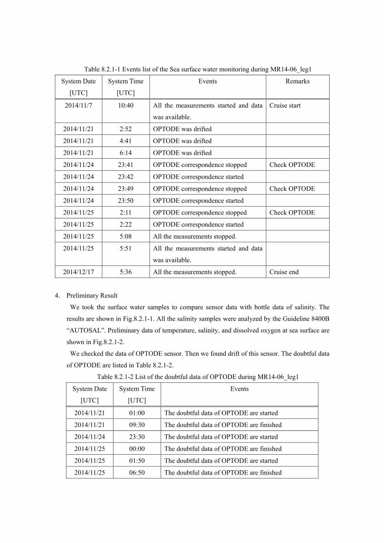
Table 8.2.1-1 Events list of the Sea surface water monitoring during MR14-06_leg1
System Date
[UTC]
System Time
[UTC]
Events Remarks
2014/11/7 10:40 All the measurements started and data
was available.
Cruise start
2014/11/21 2:52 OPTODE was drifted
2014/11/21 4:41 OPTODE was drifted
2014/11/21 6:14 OPTODE was drifted
2014/11/24 23:41 OPTODE correspondence stopped Check OPTODE
2014/11/24 23:42 OPTODE correspondence started
2014/11/24 23:49 OPTODE correspondence stopped Check OPTODE
2014/11/24 23:50 OPTODE correspondence started
2014/11/25 2:11 OPTODE correspondence stopped Check OPTODE
2014/11/25 2:22 OPTODE correspondence started
2014/11/25 5:08 All the measurements stopped.
2014/11/25 5:51 All the measurements started and data
was available.
2014/12/17 5:36 All the measurements stopped. Cruise end
4. Preliminary Result
We took the surface water samples to compare sensor data with bottle data of salinity. The
results are shown in Fig.8.2.1-1. All the salinity samples were analyzed by the Guideline 8400B
“AUTOSAL”. Preliminary data of temperature, salinity, and dissolved oxygen at sea surface are
shown in Fig.8.2.1-2.
We checked the data of OPTODE sensor. Then we found drift of this sensor. The doubtful data
of OPTODE are listed in Table 8.2.1-2.
Table 8.2.1-2 List of the doubtful data of OPTODE during MR14-06_leg1
System Date
[UTC]
System Time
[UTC]
Events
2014/11/21 01:00 The doubtful data of OPTODE are started
2014/11/21 09:30 The doubtful data of OPTODE are finished
2014/11/24 23:30 The doubtful data of OPTODE are started
2014/11/25 00:00 The doubtful data of OPTODE are finished
2014/11/25 01:50 The doubtful data of OPTODE are started
2014/11/25 06:50 The doubtful data of OPTODE are finished

5. Data archive
These data obtained in this cruise will be submitted to the Data Management Office (DMO) of
JAMSTEC, and will be opened to the public via Data Research for Whole Cruise Information in
JAMSTEC.
36
Bot
tle
35.5
35
34.5
34
33.5
y = 0.9966x + 0.1191 R² = 0.9997
33.5 34 34.5 35 35.5 36 Sensor
Fig 8.2.1-1 Correlation of salinity between sensor data and bottle data.
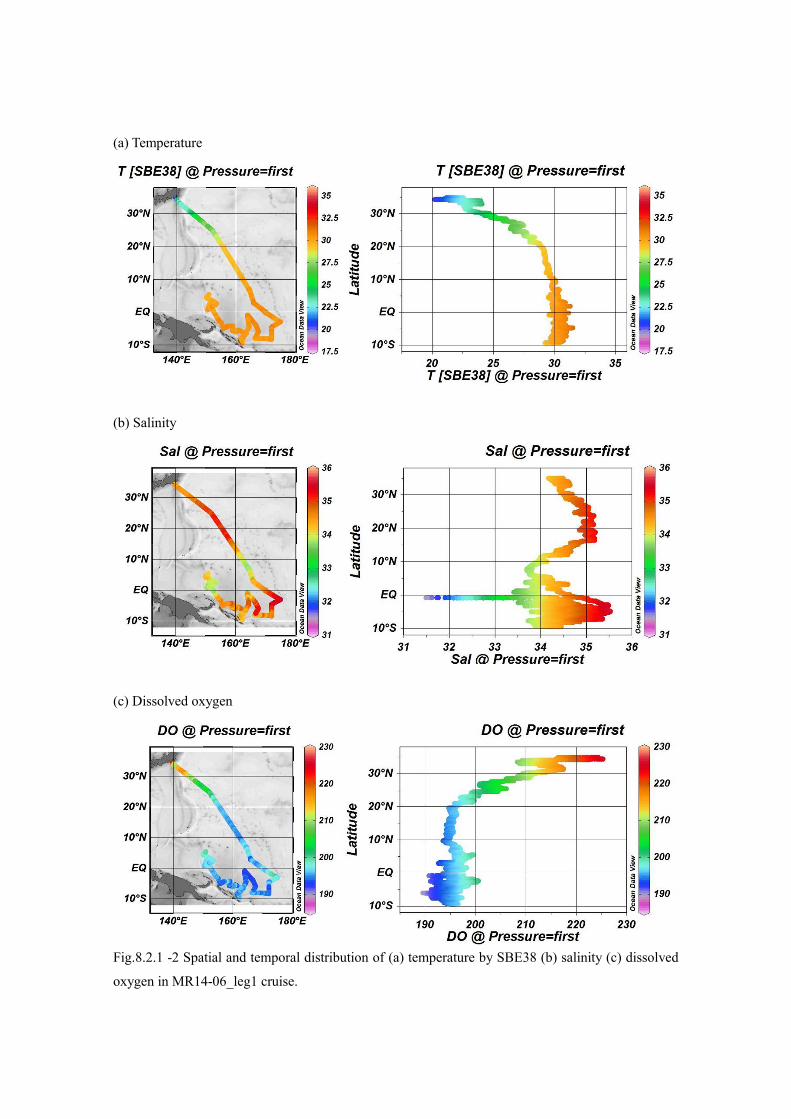
(a) Temperature
(b) Salinity
(c) Dissolved oxygen
Fig.8.2.1 -2 Spatial and temporal distribution of (a) temperature by SBE38 (b) salinity (c) dissolved
oxygen in MR14-06_leg1 cruise.
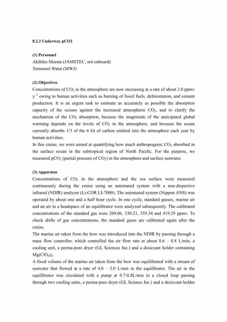
8.2.2 Underway pCO2
(1) Personnel Akihiko Murata (JAMSTEC, not onboard) Tomonori Watai (MWJ)
(2) Objectives Concentrations of CO2 in the atmosphere are now increasing at a rate of about 2.0 ppmv y–1 owing to human activities such as burning of fossil fuels, deforestation, and cement production. It is an urgent task to estimate as accurately as possible the absorption capacity of the oceans against the increased atmospheric CO2, and to clarify the mechanism of the CO2 absorption, because the magnitude of the anticipated global warming depends on the levels of CO2 in the atmosphere, and because the ocean currently absorbs 1/3 of the 6 Gt of carbon emitted into the atmosphere each year by human activities. In this cruise, we were aimed at quantifying how much anthropogenic CO2 absorbed in the surface ocean in the subtropical region of North Pacific. For the purpose, we measured pCO2 (partial pressure of CO2) in the atmosphere and surface seawater.
(3) Apparatus Concentrations of CO2 in the atmosphere and the sea surface were measured continuously during the cruise using an automated system with a non-dispersive infrared (NDIR) analyzer (Li-COR LI-7000). The automated system (Nippon ANS) was operated by about one and a half hour cycle. In one cycle, standard gasses, marine air and an air in a headspace of an equilibrator were analyzed subsequently. The calibrated concentrations of the standard gas were 269.06, 330.21, 359.34 and 419.29 ppmv. To check drifts of gas concentrations, the standard gases are calibrated again after the cruise. The marine air taken from the bow was introduced into the NDIR by passing through a mass flow controller, which controlled the air flow rate at about 0.6 – 0.8 L/min, a cooling unit, a perma-pure dryer (GL Sciences Inc.) and a desiccant holder containing Mg(ClO4)2. A fixed volume of the marine air taken from the bow was equilibrated with a stream of seawater that flowed at a rate of 4.0 – 5.0 L/min in the equilibrator. The air in the equilibrator was circulated with a pump at 0.7-0.8L/min in a closed loop passing through two cooling units, a perma-pure dryer (GL Science Inc.) and a desiccant holder
containing Mg(ClO4)2.
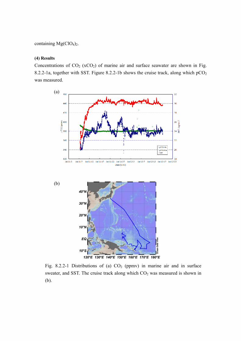
(4) Results Concentrations of CO2 (xCO2) of marine air and surface seawater are shown in Fig. 8.2.2-1a, together with SST. Figure 8.2.2-1b shows the cruise track, along which pCO2
was measured.
(a)
(b)
Fig. 8.2.2-1 Distributions of (a) CO2 (ppmv) in marine air and in surface sweater, and SST. The cruise track along which CO2 was measured is shown in (b).
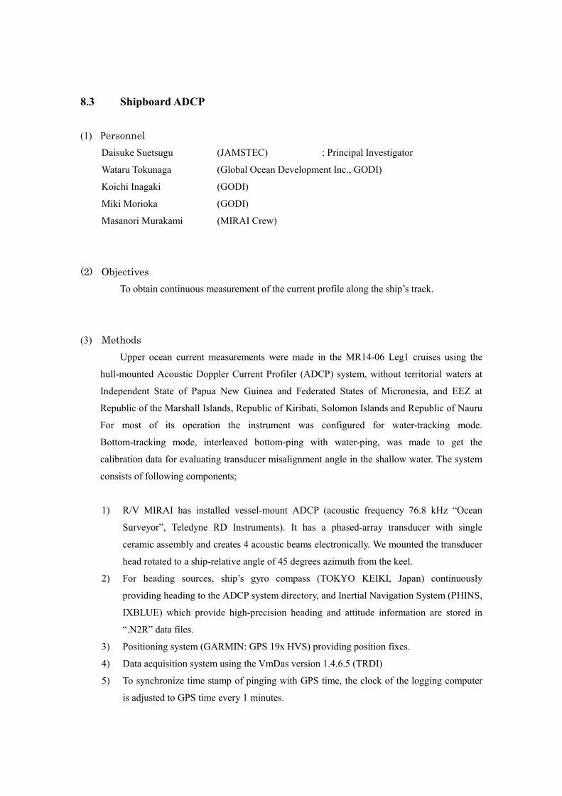
8.3 Shipboard ADCP
(1) Personnel Daisuke Suetsugu (JAMSTEC) : Principal Investigator
Wataru Tokunaga (Global Ocean Development Inc., GODI)
Koichi Inagaki (GODI)
Miki Morioka (GODI)
Masanori Murakami (MIRAI Crew)
(2) Objectives To obtain continuous measurement of the current profile along the ship’s track.
(3) Methods Upper ocean current measurements were made in the MR14-06 Leg1 cruises using the
hull-mounted Acoustic Doppler Current Profiler (ADCP) system, without territorial waters at
Independent State of Papua New Guinea and Federated States of Micronesia, and EEZ at
Republic of the Marshall Islands, Republic of Kiribati, Solomon Islands and Republic of Nauru
For most of its operation the instrument was configured for water-tracking mode.
Bottom-tracking mode, interleaved bottom-ping with water-ping, was made to get the
calibration data for evaluating transducer misalignment angle in the shallow water. The system
consists of following components;
1) R/V MIRAI has installed vessel-mount ADCP (acoustic frequency 76.8 kHz “Ocean
Surveyor”, Teledyne RD Instruments). It has a phased-array transducer with single
ceramic assembly and creates 4 acoustic beams electronically. We mounted the transducer
head rotated to a ship-relative angle of 45 degrees azimuth from the keel.
2) For heading sources, ship’s gyro compass (TOKYO KEIKI, Japan) continuously
providing heading to the ADCP system directory, and Inertial Navigation System (PHINS,
IXBLUE) which provide high-precision heading and attitude information are stored in
“.N2R” data files.
3) Positioning system (GARMIN: GPS 19x HVS) providing position fixes.
4) Data acquisition system using the VmDas version 1.4.6.5 (TRDI)
5) To synchronize time stamp of pinging with GPS time, the clock of the logging computer
is adjusted to GPS time every 1 minutes.
--------------------------------------------------------------------------------------------------------------------------
6) The sound speed at the transducer does affect the vertical bin mapping and vertical
velocity measurement, is calculated from temperature, salinity (constant value; 35.0 psu)
and depth (6.5 m; transducer depth) by equation in Medwin (1975).
Data was configured for 16 m intervals starting about 15 m below the surface. Every ping
was recorded as raw ensemble data (.ENR). Also, 60 seconds and 300 seconds averaged data
were recorded as short term average (.STA) and long term average (.LTA) data, respectively.
Major parameters for the measurement (Direct Command) are shown in Table 8.4-1.
(4) Preliminary results Fig.8.4-1 shows surface current profile along the ship’s track at research area, averaged
three depth layer from No.3 to No.5, about from 47 m to 95 m with 60 minutes averaged.
(5) Data archive These data obtained in this cruise will be submitted to the Data Management Group
(DMG) of JAMSTEC, and will be opened to the public via JAMSTEC home page.
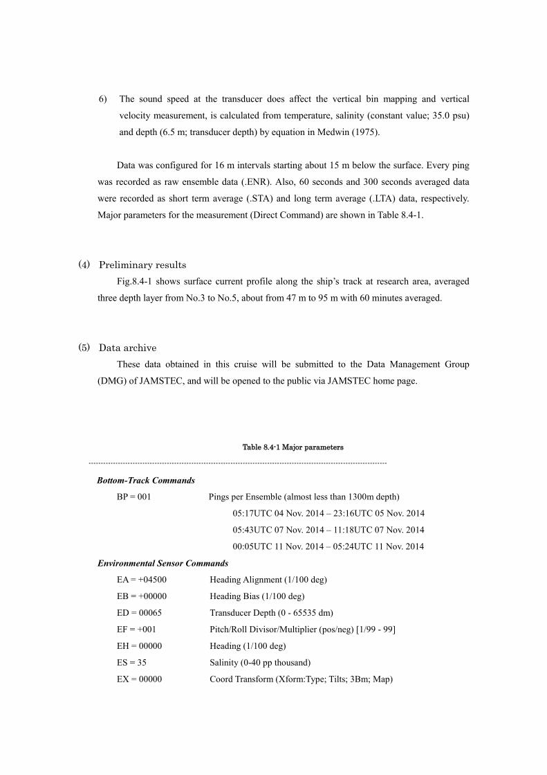
Table 8.4-1 Major parameters
Bottom-Track Commands
BP = 001 Pings per Ensemble (almost less than 1300m depth)
05:17UTC 04 Nov. 2014 – 23:16UTC 05 Nov. 2014
05:43UTC 07 Nov. 2014 – 11:18UTC 07 Nov. 2014
00:05UTC 11 Nov. 2014 – 05:24UTC 11 Nov. 2014
Environmental Sensor Commands
EA = +04500 Heading Alignment (1/100 deg)
EB = +00000 Heading Bias (1/100 deg)
ED = 00065 Transducer Depth (0 - 65535 dm)
EF = +001 Pitch/Roll Divisor/Multiplier (pos/neg) [1/99 - 99]
EH = 00000 Heading (1/100 deg)
ES = 35 Salinity (0-40 pp thousand)
EX = 00000 Coord Transform (Xform:Type; Tilts; 3Bm; Map)
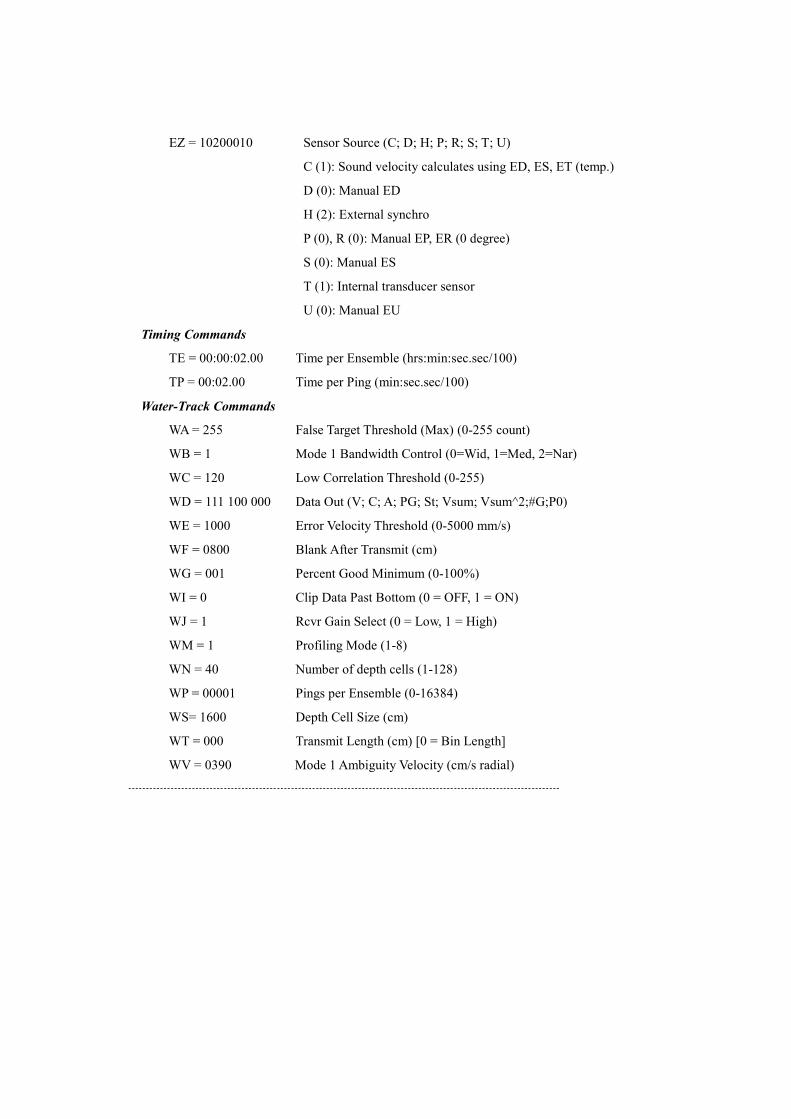
--------------------------------------------------------------------------------------------------------------------------
EZ = 10200010 Sensor Source (C; D; H; P; R; S; T; U)
C (1): Sound velocity calculates using ED, ES, ET (temp.)
D (0): Manual ED
H (2): External synchro
P (0), R (0): Manual EP, ER (0 degree)
S (0): Manual ES
T (1): Internal transducer sensor
U (0): Manual EU
Timing Commands
TE = 00:00:02.00 Time per Ensemble (hrs:min:sec.sec/100)
TP = 00:02.00 Time per Ping (min:sec.sec/100)
Water-Track Commands
WA = 255 False Target Threshold (Max) (0-255 count)
WB = 1 Mode 1 Bandwidth Control (0=Wid, 1=Med, 2=Nar)
WC = 120 Low Correlation Threshold (0-255)
WD = 111 100 000 Data Out (V; C; A; PG; St; Vsum; Vsum^2;#G;P0)
WE = 1000 Error Velocity Threshold (0-5000 mm/s)
WF = 0800 Blank After Transmit (cm)
WG = 001 Percent Good Minimum (0-100%)
WI = 0 Clip Data Past Bottom (0 = OFF, 1 = ON)
WJ = 1 Rcvr Gain Select (0 = Low, 1 = High)
WM = 1 Profiling Mode (1-8)
WN = 40 Number of depth cells (1-128)
WP = 00001 Pings per Ensemble (0-16384)
WS= 1600 Depth Cell Size (cm)
WT = 000 Transmit Length (cm) [0 = Bin Length]
WV = 0390 Mode 1 Ambiguity Velocity (cm/s radial)
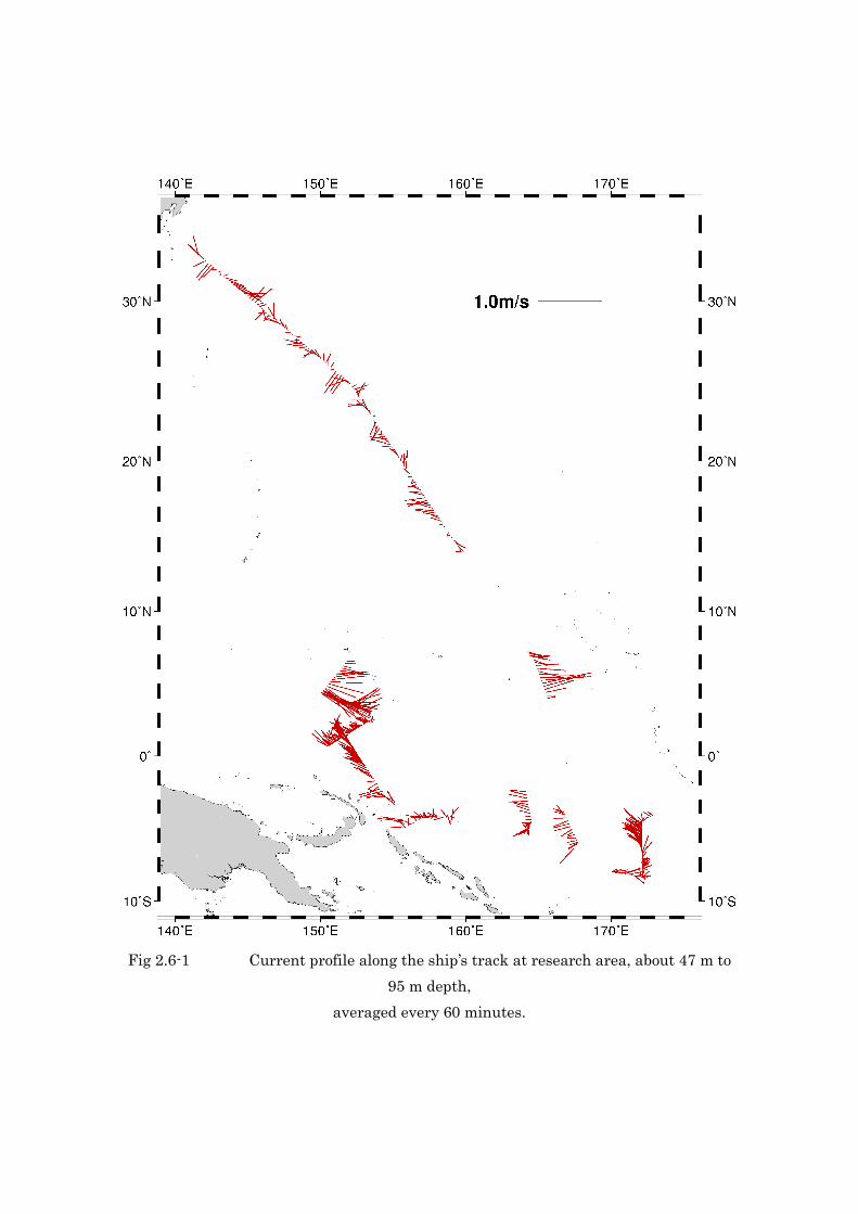
Fig 2.6-1 Current profile along the ship’s track at research area, about 47 m to95 m depth,
averaged every 60 minutes.
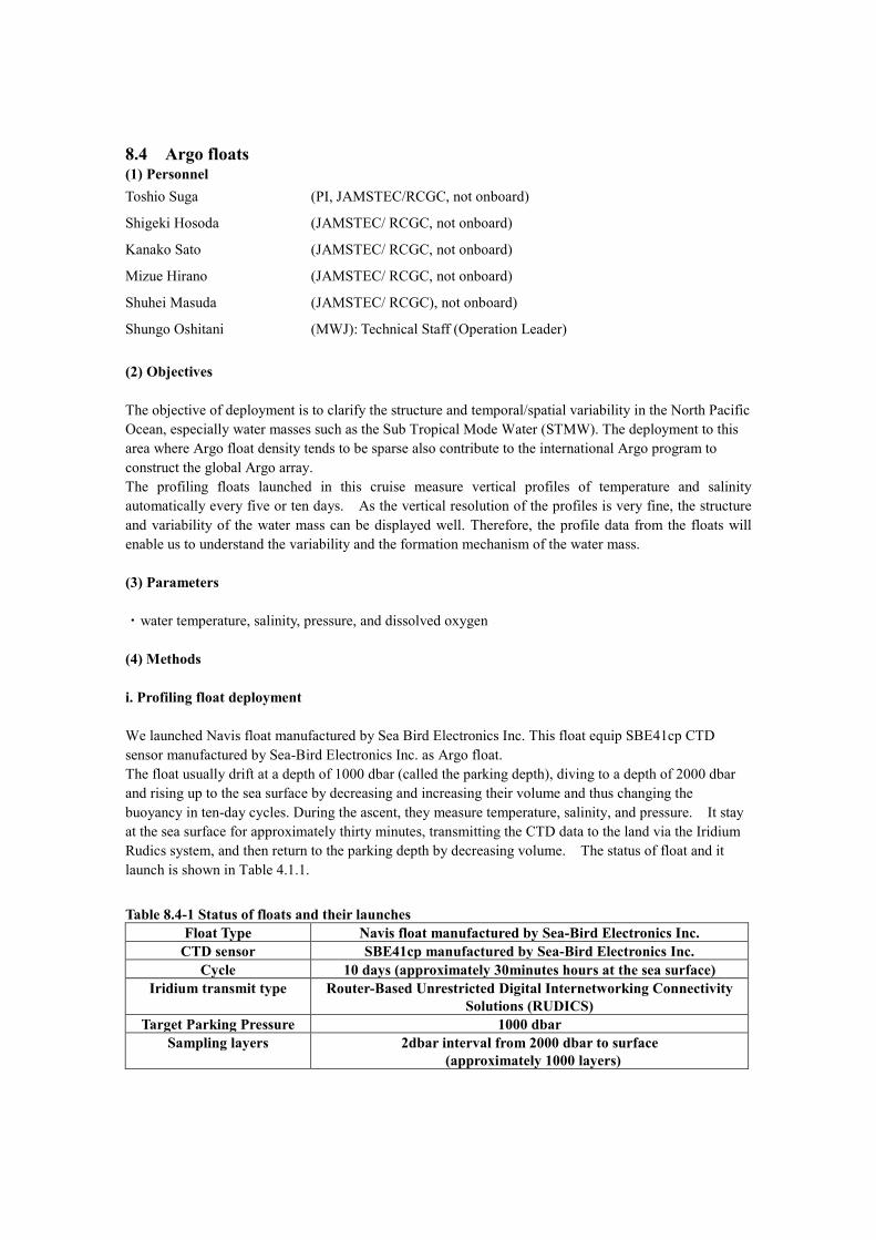
8.4 Argo floats (1) Personnel Toshio Suga (PI, JAMSTEC/RCGC, not onboard)
Shigeki Hosoda (JAMSTEC/ RCGC, not onboard)
Kanako Sato (JAMSTEC/ RCGC, not onboard)
Mizue Hirano (JAMSTEC/ RCGC, not onboard)
Shuhei Masuda (JAMSTEC/ RCGC), not onboard)
Shungo Oshitani (MWJ): Technical Staff (Operation Leader)
(2) Objectives
The objective of deployment is to clarify the structure and temporal/spatial variability in the North Pacific Ocean, especially water masses such as the Sub Tropical Mode Water (STMW). The deployment to this area where Argo float density tends to be sparse also contribute to the international Argo program to construct the global Argo array. The profiling floats launched in this cruise measure vertical profiles of temperature and salinity automatically every five or ten days. As the vertical resolution of the profiles is very fine, the structure and variability of the water mass can be displayed well. Therefore, the profile data from the floats will enable us to understand the variability and the formation mechanism of the water mass.
(3) Parameters
・water temperature, salinity, pressure, and dissolved oxygen
(4) Methods
i. Profiling float deployment
We launched Navis float manufactured by Sea Bird Electronics Inc. This float equip SBE41cp CTD sensor manufactured by Sea-Bird Electronics Inc. as Argo float. The float usually drift at a depth of 1000 dbar (called the parking depth), diving to a depth of 2000 dbar and rising up to the sea surface by decreasing and increasing their volume and thus changing the buoyancy in ten-day cycles. During the ascent, they measure temperature, salinity, and pressure. It stay at the sea surface for approximately thirty minutes, transmitting the CTD data to the land via the Iridium Rudics system, and then return to the parking depth by decreasing volume. The status of float and it launch is shown in Table 4.1.1.
Table 8.4-1 Status of floats and their launches Float Type Navis float manufactured by Sea-Bird Electronics Inc.
CTD sensor SBE41cp manufactured by Sea-Bird Electronics Inc. Cycle 10 days (approximately 30minutes hours at the sea surface)
Iridium transmit type Router-Based Unrestricted Digital Internetworking Connectivity Solutions (RUDICS)
Target Parking Pressure 1000 dbar Sampling layers 2dbar interval from 2000 dbar to surface
(approximately 1000 layers)
Launches Float S/N WMO
ID Date and Time
of Launch(UTC) Location of Launch CTD St. No.
F0398 2902531 2014/11/10 12:40 24° 59.99' [N]
152° 00.00'[E]
N/A
(5) Data archive
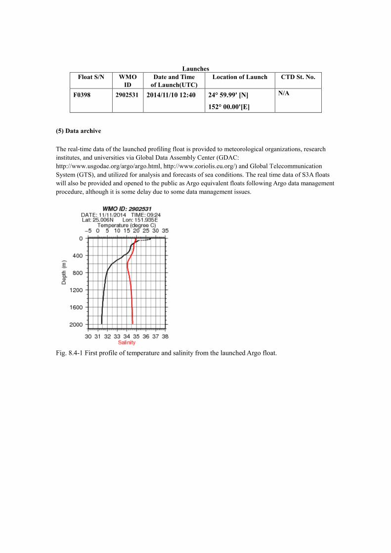
The real-time data of the launched profiling float is provided to meteorological organizations, research institutes, and universities via Global Data Assembly Center (GDAC: http://www.usgodae.org/argo/argo.html, http://www.coriolis.eu.org/) and Global Telecommunication System (GTS), and utilized for analysis and forecasts of sea conditions. The real time data of S3A floats will also be provided and opened to the public as Argo equivalent floats following Argo data management procedure, although it is some delay due to some data management issues.
Fig. 8.4-1 First profile of temperature and salinity from the launched Argo float.
8.5 Underway geophysics Personnel
Daisuke Suetsugu (JAMSTEC) : Principal Investigator
Shoka Shimizu (JAMSTEC)
Takeshi Hanyu (JAMSTEC) : Not on-board
Masao Nakanishi (Chiba University) : Not on-board
Takeshi Matsumoto (University of the Ryukyus) : Not on-board
Wataru Tokunaga (Global Ocean Development Inc., GODI)
Koichi Inagaki (GODI)
Miki Morioka (GODI)
Masanori Murakami (MIRAI Crew)
8.5.1 Sea surface gravity
(1) Introduction
The local gravity is an important parameter in geophysics and geodesy. We collected
gravity data at the sea surface during the MR14-06 Leg1 cruise without territorial waters on
Independent State of Papua New Guinea and Federated States of Micronesia.
(2) Parameters
Relative Gravity [CU: Counter Unit]
[mGal] = (coef1: 0.9946) * [CU]
(3) Data Acquisition
We measured relative gravity using LaCoste and Romberg air-sea gravity meter S-116
(Micro-g LaCoste, LLC) during this cruise. To convert the relative gravity to absolute one, we
measured gravity, using portable gravity meter (Scintrex gravity meter CG-5), at Sekinehama as
the reference point.
(4) Preliminary Results
Absolute gravity shown in Table 8.5.1-1
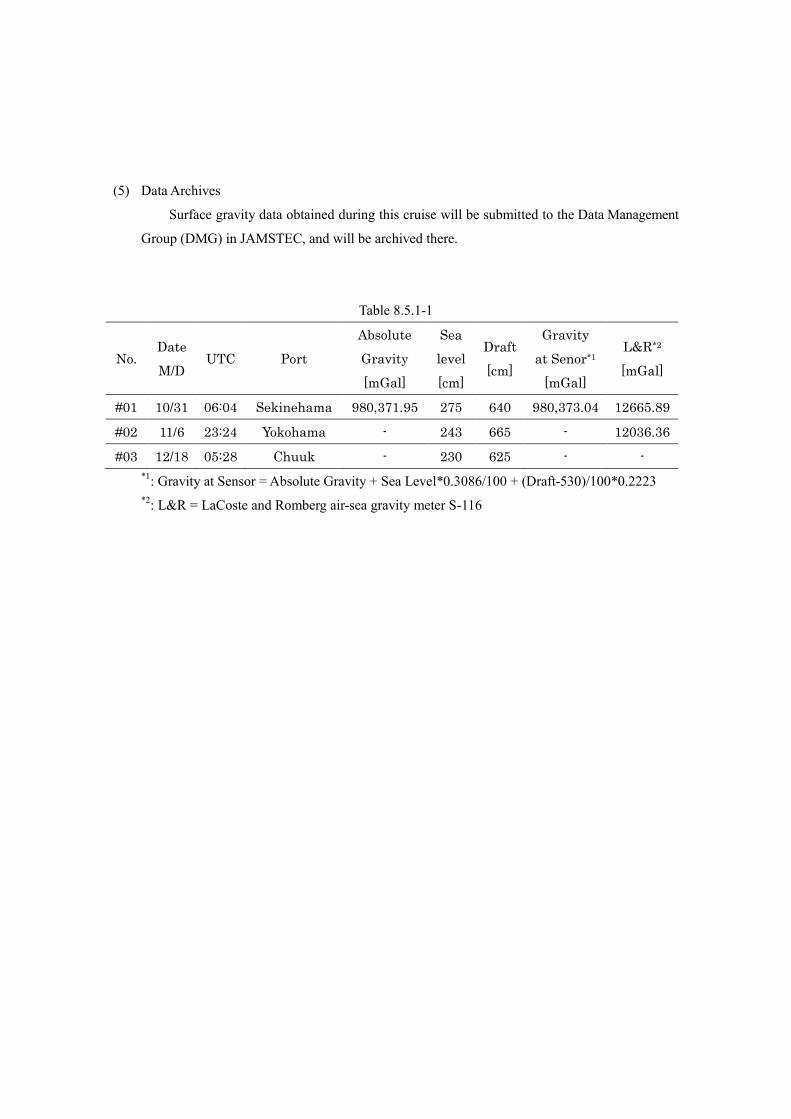
(5) Data Archives
Surface gravity data obtained during this cruise will be submitted to the Data Management
Group (DMG) in JAMSTEC, and will be archived there.
Table 8.5.1-1
Absolute Sea Gravity Date Draft L&R*2
No. UTC Port Gravity level at Senor*1 M/D [cm] [mGal]
[mGal] [cm] [mGal]
#01 10/31 06:04 Sekinehama 980,371.95 275 640 980,373.04 12665.89
#02 11/6 23:24 Yokohama - 243 665 - 12036.36
#03 12/18 05:28 Chuuk - 230 625 - -*1: Gravity at Sensor = Absolute Gravity + Sea Level*0.3086/100 + (Draft-530)/100*0.2223 *2: L&R = LaCoste and Romberg air-sea gravity meter S-116
8.5.2 Sea surface magnetic field
1) Three-component magnetometer
(1) Introduction Measurement of magnetic force on the sea is required for the geophysical investigations of
marine magnetic anomaly caused by magnetization in upper crustal structure. We measured
geomagnetic field using a three-component magnetometer during the MR14-06 Leg1 cruise
without territorial waters on Independent State of Papua New Guinea and Federated States of
Micronesia.
(2) Principle of ship-board geomagnetic vector measurement
The relation between a magnetic-field vector observed on-board, Hob, (in the ship's fixed
coordinate system) and the geomagnetic field vector, F, (in the Earth's fixed coordinate system) is
expressed as:
Hob = A R P Y F + Hp (a)
where R, P and Y are the matrices of rotation due to roll, pitch and heading of a ship,
respectively. A is a 3 x 3 matrix which represents magnetic susceptibility of the ship, and Hp is a magnetic field vector produced by a permanent magnetic moment of the ship's body.
Rearrangement of Eq. (a) makes
F (b)
where R = A -1, and Hbp = -R Hp. The magnetic field, F, can be obtained by measuring
Hob + Hbp =R R P Y
R , P , Y and Hob, if R and Hbp are known. Twelve constants in R and Hbp can be
determined by measuring variation of Hob with R , P and Y at a place where the geomagnetic field, F, is known.
(3) Instruments on R/V MIRAI
A shipboard three-component magnetometer system (Tierra Tecnica SFG1214) is equipped
on-board R/V MIRAI. Three-axes flux-gate sensors with ring-cored coils are fixed on the fore
mast. Outputs from the sensors are digitized by a 20-bit A/D converter (1 nT/LSB), and sampled
at 8 times per second. Ship's heading, pitch, and roll are measured by the Inertial Navigation System (INS) for controlling attitude of a Doppler radar. Ship's position (GPS) and speed data
are taken from LAN every second.
(4) Data Archives
These data obtained in this cruise will be submitted to the Data Management Group (DMG)
of JAMSTEC.
(5) Remarks
1) For calibration of the ship’s magnetic effect, we made a “figure-eight” turn (a pair of
clockwise and anti-clockwise rotation). This calibration was carried out as below.
01:11 – 01:47 15 Nov. 2014 around 06-57N, 164-30E
23:27 – 23:53 18 Nov. 2014 around 02-58S, 175-00E
11:44 – 12:09 27 Nov. 2014 around 03-53S, 166-43E
10:05 – 10:28 04 Dec. 2014 around 06-24S, 163-25E
12:36 – 12:59 09 Dec. 2014 around 00-37S, 152-59E
2) Cesium magnetometer
(1) Introduction
Measurement of total magnetic force on the sea is required for the geophysical
investigations of marine magnetic anomaly caused by magnetization in upper crustal structure.
(2) Data Period and Sensor Rotation
20:58 19 Nov. 2014 – 01:08 23 Nov. 2014 Rotation = 0 degrees
09:18 24 Nov. 2014 – 04:16 25 Nov. 2014 Rotation = 0 degrees
08:32 25 Nov. 2014 – 20:52 26 Nov. 2014 Rotation = +30 degrees
10:27 29 Nov. 2014 – 22:32 03 Dec. 2014 Rotation = 0 degrees
15:48 04 Dec. 2014 – 22:48 05 Dec. 2014 Rotation = +75 degrees
09:44 06 Dec. 2014 – 03:07 07 Dec. 2014 Rotation = 0 degrees
08:05 07 Dec. 2014 – 22:54 07 Dec. 2014 Rotation = -30 degrees
23:10 07 Dec. 2014 – 09:41 08 Dec. 2014 Rotation = 0 degrees
17:50 08 Dec. 2014 – 23:19 08 Dec. 2014 Rotation = 0 degrees
15:05 09 Dec. 2014 – 10:08 12 Dec. 2014 Rotation = +135 degrees
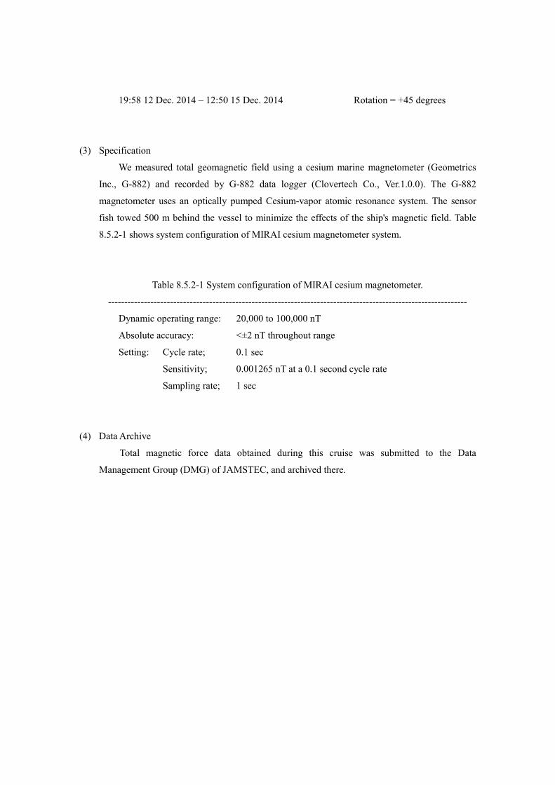
--------------------------------------------------------------------------------------------------------------
19:58 12 Dec. 2014 – 12:50 15 Dec. 2014 Rotation = +45 degrees
(3) Specification
We measured total geomagnetic field using a cesium marine magnetometer (Geometrics
Inc., G-882) and recorded by G-882 data logger (Clovertech Co., Ver.1.0.0). The G-882
magnetometer uses an optically pumped Cesium-vapor atomic resonance system. The sensor
fish towed 500 m behind the vessel to minimize the effects of the ship's magnetic field. Table
8.5.2-1 shows system configuration of MIRAI cesium magnetometer system.
Table 8.5.2-1 System configuration of MIRAI cesium magnetometer.
Dynamic operating range: 20,000 to 100,000 nT
Absolute accuracy: <±2 nT throughout range
Setting: Cycle rate; 0.1 sec
Sensitivity; 0.001265 nT at a 0.1 second cycle rate
Sampling rate; 1 sec
(4) Data Archive
Total magnetic force data obtained during this cruise was submitted to the Data
Management Group (DMG) of JAMSTEC, and archived there.
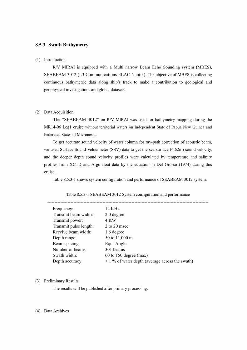
---------------------------------------------------------------------------------------------------------------
8.5.3 Swath Bathymetry
(1) Introduction
R/V MIRAI is equipped with a Multi narrow Beam Echo Sounding system (MBES),
SEABEAM 3012 (L3 Communications ELAC Nautik). The objective of MBES is collecting
continuous bathymetric data along ship’s track to make a contribution to geological and
geophysical investigations and global datasets.
(2) Data Acquisition
The “SEABEAM 3012” on R/V MIRAI was used for bathymetry mapping during the
MR14-06 Leg1 cruise without territorial waters on Independent State of Papua New Guinea and
Federated States of Micronesia.
To get accurate sound velocity of water column for ray-path correction of acoustic beam,
we used Surface Sound Velocimeter (SSV) data to get the sea surface (6.62m) sound velocity,
and the deeper depth sound velocity profiles were calculated by temperature and salinity
profiles from XCTD and Argo float data by the equation in Del Grosso (1974) during this
cruise.
Table 8.5.3-1 shows system configuration and performance of SEABEAM 3012 system.
Table 8.5.3-1 SEABEAM 3012 System configuration and performance
Frequency: 12 KHz Transmit beam width: 2.0 degree Transmit power: 4 KW Transmit pulse length: 2 to 20 msec. Receive beam width: 1.6 degree Depth range: 50 to 11,000 m Beam spacing: Equi-Angle Number of beams 301 beams Swath width: 60 to 150 degree (max) Depth accuracy: < 1 % of water depth (average across the swath)
(3) Preliminary Results
The results will be published after primary processing.
(4) Data Archives

Bathymetric data obtained during this cruise will be submitted to the Data Management
Group (DMG) in JAMSTEC, and will be archived there.
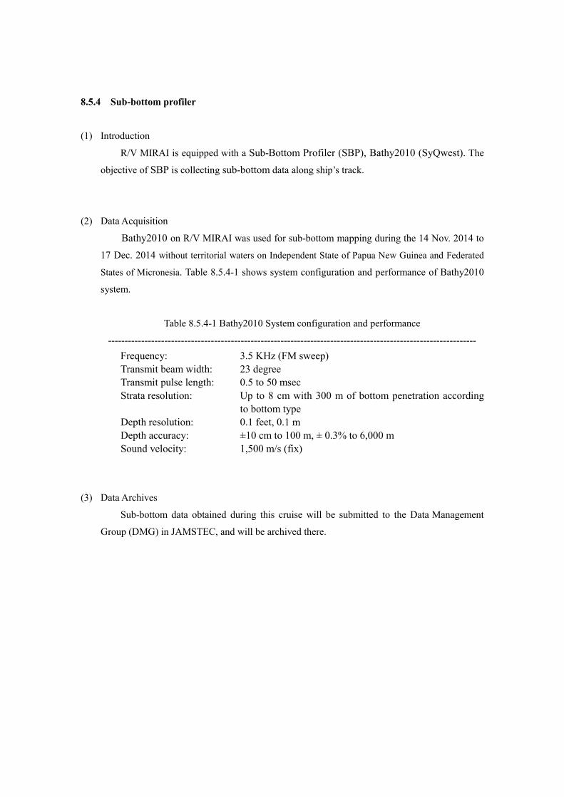
---------------------------------------------------------------------------------------------------------------
8.5.4 Sub-bottom profiler
(1) Introduction
R/V MIRAI is equipped with a Sub-Bottom Profiler (SBP), Bathy2010 (SyQwest). The
objective of SBP is collecting sub-bottom data along ship’s track.
(2) Data Acquisition
Bathy2010 on R/V MIRAI was used for sub-bottom mapping during the 14 Nov. 2014 to
17 Dec. 2014 without territorial waters on Independent State of Papua New Guinea and Federated
States of Micronesia. Table 8.5.4-1 shows system configuration and performance of Bathy2010
system.
Table 8.5.4-1 Bathy2010 System configuration and performance
Frequency: 3.5 KHz (FM sweep) Transmit beam width: 23 degree Transmit pulse length: 0.5 to 50 msec Strata resolution: Up to 8 cm with 300 m of bottom penetration according
to bottom type Depth resolution: 0.1 feet, 0.1 m Depth accuracy: ±10 cm to 100 m, ± 0.3% to 6,000 m Sound velocity: 1,500 m/s (fix)
(3) Data Archives
Sub-bottom data obtained during this cruise will be submitted to the Data Management
Group (DMG) in JAMSTEC, and will be archived there.
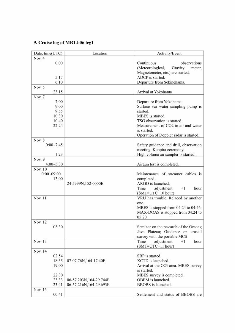
9. Cruise log of MR14-06 leg1
Date, time(UTC) Location Activity/Event Nov. 4
0:00 Continuous observations (Meteorological, Gravity meter, Magnetometer, etc.) are started.
5:17 ADCP is started. 6:10 Departure from Sekinehama.
Nov. 5 23:15 Arrival at Yokohama
Nov. 7 7:00 Departure from Yokohama. 9:00 Surface sea water sampling pump is 9:55 started.
10:30 MBES is started. 10:40 TSG observation is started. 22:24 Measurement of CO2 in air and water
is started. Operation of Doppler radar is started.
Nov. 8 0:00~7:45 Safety guidance and drill, observation
meeting, Konpira ceremony. 1:23 High volume air sampler is started.
Nov. 9 4:00~5:30 Airgun test is completed.
Nov. 10 0:00~09:00 Maintenance of streamer cables is
13:00 completed. 24-5999N,152-0000E ARGO is launched.
Time adjustment +1 hour (SMT=UTC+10 hour)
Nov. 11 VRU has trouble. Relaced by another one. MBES is stopped from 04:24 to 04:46. MAX-DOAS is stopped from 04:24 to 05:20.
Nov. 12 03:30 Seminar on the research of the Ontong
Java Plateau; Guidance on crustal survey with the portable MCS
Nov. 13 Time adjustment +1 hour (SMT=UTC+11 hour)
Nov. 14 02:54 SBP is started. 18:35 07-07.76N,164-17.40E XCTD is launched. 19:00 Arrival at the O23 area. MBES survey
is started. 22:30 MBES survey is completed. 23:33 06-57.203N,164-29.744E OBEM is launched. 23:41 06-57.216N,164-29.693E BBOBS is launched.
Nov. 15 00:41 Settlement and status of BBOBS are
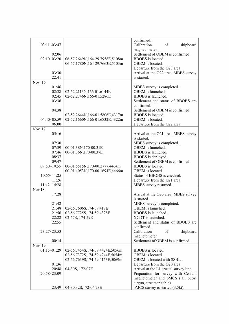
confirmed. 03:11~03:47 Calibration of shipboard
magnetometer 02:06 Settlement of OBEM is confirmed.
02:10~03:20 06-57.2649N,164-29.7958E,5108m BBOBS is located. 06-57.1780N,164-29.7663E,5103m OBEM is located.
Departure from the O23 area 03:30 Arrival at the O22 area. MBES survey 22:41 is started.
Nov. 16 01:46 MBES survey is completed. 02:38 02-52.2113N,166-01.6144E OBEM is launched. 02:45 02-52.2746N,166-01.5286E BBOBS is launched. 03:36 Settlement and status of BBOBS are
confirmed. 04:38 Settlement of OBEM is confirmed.
02-52.2644N,166-01.5806E,4317m BBOBS is located. 04:40~05.59 02-52.1660N,166-01.6832E,4322m OBEM is located.
06:00 Departure from the O22 area Nov. 17
05:16 Arrival at the O21 area. MBES survey is started.
07:30 MBES survey is completed. 07:39 00-01.38N,170-00.31E OBEM is launched. 07:46 00-01.36N,170-00.37E BBOBS is launched. 08:37 BBOBS is deployed. 09:47 Settlement of OBEM is confirmed.
09:50~10:55 00-01.5515N,170-00.2777,4464m BBOBS is located. 00-01.4053N,170-00.1694E,4466m OBEM is located.
10:55~11:25 Status of BBOBS is checked. 11:26 Departure from the O21 area
11:42~14:28 MBES survey resumed. Nov.18
17:28 Arrival at the O20 area. MBES survey is started.
21:42 MBES survey is completed. 21:48 02-56.7606S,174-59.417E OBEM is launched. 21:56 02-56.7725S,174-59.4328E BBOBS is launched. 22:22 02-57S, 174-59E XCDT is launched. 22:55 Settlement and status of BBOBS are
confirmed. 23:27~23:53 Calibration of shipboard
magnetometer. 00:14 Settlement of OBEM is confirmed.
Nov. 19 01:15~01:29 02-56.7454S,174-59.4424E,5056m BBOBS is located.
02-56.7372S,174-59.4244E,5054m OBEM is located. 02-56.7639S,174-59.4153E,5069m OBEM is located with SSBL.
01:36 Departure from the O20 area 20:48 04-30S, 172-07E Arrival at the L1 crustal survey line
20:58~23:09 Preparation for survey with Cesium magnetometer and pMCS (tail buoy, airgun, streamer cable)
23:49 04-30.32S,172-06.73E pMCS survey is started (3.5kt).
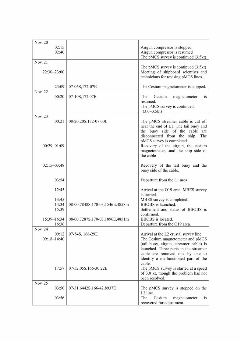
Nov. 20 02:15 Airgun compressor is stopped 02:40 Airgun compressor is resumed
The pMCS survey is continued (3.5kt) Nov. 21
The pMCS survey is continued (3.5kt) 22:30~23:00 Meeting of shipboard scientists and
technicians for revising pMCS lines.
23:09 07-06S,172-07E The Cesium magnetometer is stopped. Nov. 22
00:20 07-10S,172.07E The Cesium magnetometer is resumed. The pMCS survey is continued. (3.0~3.5kt)
Nov. 23 00:21 08-20.20S,172-07.00E The pMCS streamer cable is cut off
near the end of L1. The tail buoy and the buoy side of the cable are disconnected from the ship. The pMCS survey is completed.
00:29~01:09 Recovery of the airgun, the cesium magnetometer, .and the ship side of the cable
02:15~03:48 Recovery of the tail buoy and the buoy side of the cable.
03:54 Departure from the L1 area
12:45 Arrival at the O19 area. MBES survey is started.
13:45 MBES survey is completed. 14:34 08-00.7848S,170-03.1546E,4858m BBOBS is launched. 15:39 Settlement and status of BBOBS is
confirmed. 15:39~16:34 08-00.7287S,170-03.1896E,4851m BBOBS is located.
16:36 Departure from the O19 area. Nov. 24
09:12 07-54S, 166-29E Arrival at the L2 crustal survey line 09:18~14:40 The Cesium magnetometer and pMCS
(tail buoy, airgun, streamer cable) is launched. Three parts in the streamer cable are removed one by one to identify a malfunctioned part of the cable.
17:57 07-52.05S,166-30.22E The pMCS survey is started at a speed of 3.0 kt, though the problem has not been resolved.
Nov. 25 03:50 07-31.6442S,166-42.8937E The pMCS survey is stopped on the
L2 line. 03:56 The Cesium magnetometer is
recovered for adjustment.
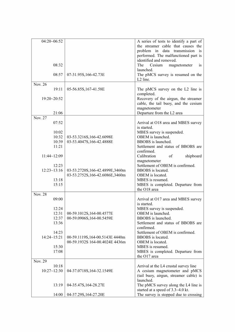
04:20~06:52 A series of tests to identify a part of the streamer cable that causes the problem in data transmission is performed. The malfunctioned part is identified and removed.
08:32 The Cesium magnetometer is launched.
08:57 07-31.95S,166-42.73E The pMCS survey is resumed on the L2 line.
Nov. 26 19:11 05-56.85S,167-41.58E The pMCS survey on the L2 line is
completed. 19:20~20:52 Recovery of the airgun, the streamer
cable, the tail buoy, and the cesium magnetometer
21:06 Departure from the L2 area Nov. 27
07:52 Arrival at O18 area and MBES survey is started.
10:02 MBES survey is suspended. 10:32 03-53.3216S,166-42.6098E OBEM is launched. 10:39 03-53.4047S,166-42.4888E BBOBS is launched. 11:21 Settlement and status of BBOBS are
confirmed. 11:44~12:09 Calibration of shipboard
magnetometer 12:23 Settlement of OBEM is confirmed.
12:23~13:16 03-53.2720S,166-42.4899E,3460m BBOBS is located. 03-53.2752S,166-42.6086E,3460m OBEM is located.
13:18 MBES is resumed. 15:15 MBES is completed. Departure from
the O18 area Nov. 28
09:00 Arrival at O17 area and MBES survey is started.
12:24 MBES survey is suspended. 12:31 00-59.1012S,164-00.4577E OBEM is launched. 12:37 00-59.0906S,164-00.5459E BBOBS is launched. 13:36 Settlement and status of BBOBS are
confirmed. 14:23 Settlement of OBEM is confirmed.
14:24~15:21 00-59.1119S,164-00.5143E 4440m BBOBS is located. 00-59.1932S 164-00.4024E 4436m OBEM is located.
15:30 MBES is resumed. 17:08 MBES is completed. Departure from
the O17 area Nov. 29
10:18 Arrival at the L4 crustal survey line 10:27~12:30 04-37.0718S,164-32.1549E A cesium magnetometer and pMCS
(tail buoy, airgun, streamer cable) is launched.
13:19 04-35.47S,164-28.27E The pMCS survey along the L4 line is started at a speed of 3.3~4.0 kt.
14:00 04-37.29S,164-27.20E The survey is stopped due to crossing
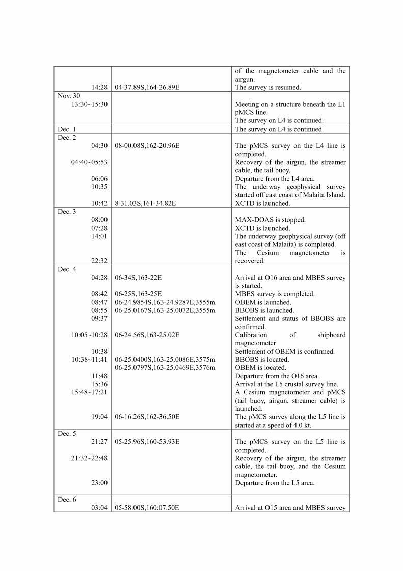
14:28 04-37.89S,164-26.89E
of the magnetometer cable and the airgun. The survey is resumed.
Nov. 30 13:30~15:30 Meeting on a structure beneath the L1
pMCS line. The survey on L4 is continued.
Dec. 1 The survey on L4 is continued. Dec. 2
04:30 08-00.08S,162-20.96E The pMCS survey on the L4 line is completed.
04:40~05:53 Recovery of the airgun, the streamer cable, the tail buoy.
06:06 Departure from the L4 area. 10:35 The underway geophysical survey
started off east coast of Malaita Island. 10:42 8-31.03S,161-34.82E XCTD is launched.
Dec. 3 08:00 MAX-DOAS is stopped. 07:28 XCTD is launched. 14:01 The underway geophysical survey (off
east coast of Malaita) is completed. The Cesium magnetometer is
22:32 recovered. Dec. 4
04:28 06-34S,163-22E Arrival at O16 area and MBES survey is started.
08:42 06-25S,163-25E MBES survey is completed. 08:47 06-24.9854S,163-24.9287E,3555m OBEM is launched. 08:55 06-25.0167S,163-25.0072E,3555m BBOBS is launched. 09:37 Settlement and status of BBOBS are
confirmed. 10:05~10:28 06-24.56S,163-25.02E Calibration of shipboard
magnetometer 10:38 Settlement of OBEM is confirmed.
10:38~11:41 06-25.0400S,163-25.0086E,3575m BBOBS is located. 06-25.0797S,163-25.0469E,3576m OBEM is located.
11:48 Departure from the O16 area. 15:36 Arrival at the L5 crustal survey line.
15:48~17:21 A Cesium magnetometer and pMCS (tail buoy, airgun, streamer cable) is launched.
19:04 06-16.26S,162-36.50E The pMCS survey along the L5 line is started at a speed of 4.0 kt.
Dec. 5 21:27 05-25.96S,160-53.93E The pMCS survey on the L5 line is
completed. 21:32~22:48 Recovery of the airgun, the streamer
cable, the tail buoy, and the Cesium magnetometer.
23:00 Departure from the L5 area.
Dec. 6 03:04 05-58.00S,160:07.50E Arrival at O15 area and MBES survey
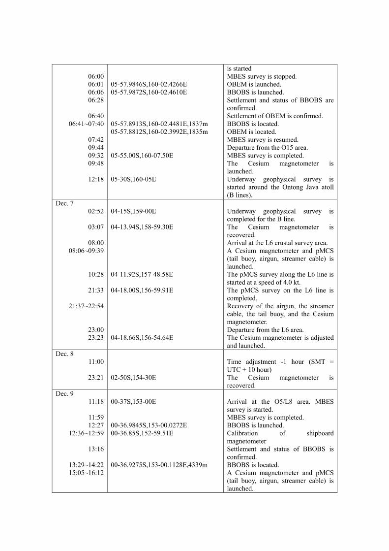
is started 06:00 MBES survey is stopped. 06:01 05-57.9846S,160-02.4266E OBEM is launched. 06:06 05-57.9872S,160-02.4610E BBOBS is launched. 06:28 Settlement and status of BBOBS are
confirmed. 06:40 Settlement of OBEM is confirmed.
06:41~07:40 05-57.8913S,160-02.4481E,1837m BBOBS is located. 05-57.8812S,160-02.3992E,1835m OBEM is located.
07:42 MBES survey is resumed. 09:44 Departure from the O15 area. 09:32 05-55.00S,160-07.50E MBES survey is completed. 09:48 The Cesium magnetometer is
launched. 12:18 05-30S,160-05E Underway geophysical survey is
started around the Ontong Java atoll (B lines).
Dec. 7 02:52 04-15S,159-00E Underway geophysical survey is
completed for the B line. 03:07 04-13.94S,158-59.30E The Cesium magnetometer is
recovered. 08:00 Arrival at the L6 crustal survey area.
08:06~09:39 A Cesium magnetometer and pMCS (tail buoy, airgun, streamer cable) is launched.
10:28 04-11.92S,157-48.58E The pMCS survey along the L6 line is started at a speed of 4.0 kt.
21:33 04-18.00S,156-59.91E The pMCS survey on the L6 line is completed.
21:37~22:54 Recovery of the airgun, the streamer cable, the tail buoy, and the Cesium magnetometer.
23:00 Departure from the L6 area. 23:23 04-18.66S,156-54.64E The Cesium magnetometer is adjusted
and launched. Dec. 8
11:00 Time adjustment -1 hour (SMT = UTC + 10 hour)
23:21 02-50S,154-30E The Cesium magnetometer is recovered.
Dec. 9 11:18 00-37S,153-00E Arrival at the O5/L8 area. MBES
survey is started. 11:59 MBES survey is completed. 12:27 00-36.9845S,153-00.0272E BBOBS is launched.
12:36~12:59 00-36.85S,152-59.51E Calibration of shipboard magnetometer
13:16 Settlement and status of BBOBS is confirmed.
13:29~14:22 00-36.9275S,153-00.1128E,4339m BBOBS is located. 15:05~16:12 A Cesium magnetometer and pMCS
(tail buoy, airgun, streamer cable) is launched.

17:22 00-37.49S,153-00.33E The pMCS survey along the L8 line is started at a speed of 3.0 kt.
Dec. 10 04:51 00-08.86S,152-42.06E The pMCS survey is stopped on the
L8 line. 04:52~06:25 The malfunctioned part is identified
and removed. 08:43 00-10.57S,152-43.15E The pMCS survey is resumed on the
L8 line. Dec. 11 The pMCS is continued on L8. Dec. 12
05:02 02:19.38N,151-07.40E The pMCS survey is completed on L8. 05:05~10:12 Recovery of the airgun, the streamer
cable, the tail buoy, and the Cesium magnetometer. During the recovery, malfunctioned parts of the active cable are identified and removed and stretch cables are added.
10:24 Departure from the L8 area 19:54 00-40.21N,150-27.30E Arrival at the L7 crustal survey line.
19:58~21:31 A Cesium magnetometer and pMCS (tail buoy, airgun, streamer cable) is launched.
22:20 00-40.96N,150-31.93E The pMCS survey along the L7 line is started at a speed of 4.0 kt.
Dec. 13 10:25 MAX-DOAS is resumed. 21:00 Disdrometer is stopped due to disk
full. The pMCS survey is continued.
Dec. 14 12:30 Survey speed is reduced to 3.0 kt.
The pMCS survey is continued. 13:00 Disdrometer is resumed.
Dec. 15 11:01 02-35.54N,153-34.33E The pMCS survey on the L7 line is
completed. 11:04~12:51 Recovery of the airgun, the streamer
cable, the tail buoy, and the Cesium magnetometer.
13:12 Departure from the L7 area. Dec. 16 06:32 04-15.00N,150-25.00E Arrival at O4 area and MBES survey
is started. 11:06 MBES survey is stopped. 11:10 04-26.9833N,150-23.0112E OBEM is launched. 11:17 04-27.0324N,150-22.9174E BBOBS is launched. 12:04 Settlement and status of BBOBS are
confirmed. 12:24~12:44 04-26.55N,150-23.55E Calibration of shipboard
magnetometer 13:07 Settlement of OBEM is confirmed. 13:08~14:12 04-27.0003N 150-22.9776E 4008m BBOBS is located.
04-26.9613N 150-23.0580E 4006m OBEM is located.
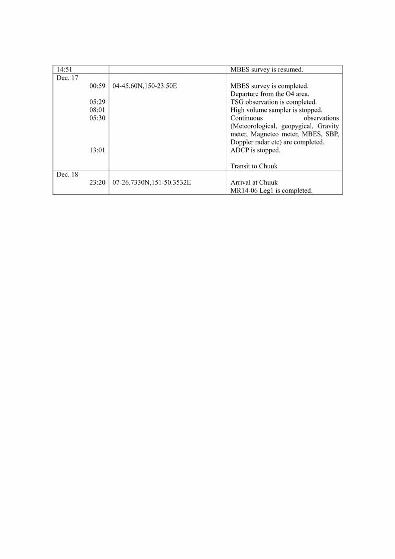
14:51 MBES survey is resumed. Dec. 17
00:59 04-45.60N,150-23.50E MBES survey is completed. Departure from the O4 area.
05:29 TSG observation is completed. 08:01 High volume sampler is stopped. 05:30 Continuous observations
(Meteorological, geopygical, Gravity meter, Magneteo meter, MBES, SBP, Doppler radar etc) are completed.
13:01 ADCP is stopped.
Transit to Chuuk Dec. 18
23:20 07-26.7330N,151-50.3532E Arrival at Chuuk MR14-06 Leg1 is completed.