Mining Road Network Correlation for Trafﬁc Estimation ... · Mining Road Network Correlation for...

1880 IEEE TRANSACTIONS ON INTELLIGENT TRANSPORTATION SYSTEMS, VOL. 17, NO. 7, JULY 2016

Mining Road Network Correlation for TrafficEstimation via Compressive Sensing

Zhidan Liu, Member, IEEE, Zhenjiang Li, Member, IEEE, Mo Li, Member, IEEE, Wei Xing, and Dongming Lu

Abstract—This paper presents a transport traffic estimationmethod which leverages road network correlation and sparsetraffic sampling via the compressive sensing technique. Throughthe investigation on a traffic data set of more than 4400 taxisfrom Shanghai city, China, we observe nontrivial traffic corre-lations among the traffic conditions of different road segmentsand derive a mathematical model to capture such relations. Aftermathematical manipulation, the models can be used to constructrepresentation bases to sparsely represent the traffic conditionsof all road segments in a road network. With the trait of sparserepresentation, we propose a traffic estimation approach thatapplies the compressive sensing technique to achieve a city-scaletraffic estimation with only a small number of probe vehicles,largely reducing the system operating cost. To validate the trafficcorrelation model and estimation method, we do extensive trace-driven experiments with real-world traffic data. The results showthat the model effectively reveals the hidden structure of trafficcorrelations. The proposed estimation method derives accuratetraffic conditions with the average accuracy as 0.80, calculatedas the ratio between the number of correct traffic state categoryestimations and the number of all estimation times, based on only50 probe vehicles’ intervention, which significantly outperformsthe state-of-the-art methods in both cost and traffic estimationaccuracy.

Index Terms—Correlation modeling, traffic estimation, com-pressive sensing.

I. INTRODUCTION

UNDERSTANDING traffic conditions is crucial in urbancities, which used to incur heavy road infrastructure con-

structions, e.g., inductive loop detectors [8], and close-circuitcameras [18]. Due to the high deploying costs, however, it

Manuscript received May 18, 2015; revised September 22, 2015; acceptedDecember 28, 2015. Date of publication January 25, 2016; date of currentversion June 24, 2016. This work was supported in part by Singapore MOEAcRF under Grant MOE2012-T2-1-070 and Grant MOE2013-T1-002-005,by the NTU NAP under Grant M4080738.020, by the NSFC under Grant61303233, by the City University of Hong Kong under Project 7200480/CS,and by the National Key Research and Development Program under Grant2014BAG01B02 and Grant 2014BAG01B03. The Associate Editor for thispaper was H. Van Lint.

Z. Liu was with the College of Computer Science and Technology, ZhejiangUniversity, Hangzhou 310027, China. He is now with the School of ComputerEngineering, Nanyang Technological University, Singapore 639798 (e-mail:[email protected]).

Z. Li is with the Department of Computer Science, City University of HongKong, Kowloon, Hong Kong (e-mail: [email protected]).

M. Li is with the School of Computer Engineering, Nanyang TechnologicalUniversity, Singapore 639798 (e-mail: [email protected]).

W. Xing and D. Lu are with the College of Computer Science and Technol-ogy, Zhejiang University, Hangzhou 310027, China (e-mail: [email protected]; [email protected]).

Color versions of one or more of the figures in this paper are available onlineat http://ieeexplore.ieee.org.

Digital Object Identifier 10.1109/TITS.2016.2514519

is prohibitive to densely adopt them in the city scale, whichlargely limits the coverage. Recent studies leverage roving ve-hicles on roads as probes to estimate the traffic conditions [11],[24], [30]. Vehicles, equipped with GPS, can periodically reporttheir current locations, driving speeds or directions via certaindata delivery scheme [14]. With such on-site traffic information,we can instantly estimate traffic speeds of the roads coveredby probe vehicles. For example, Google employs probe carsto measure road speeds and summarizes the traffic speeds ofdifferent roads on Google Map. Using roving vehicles largelyextends the coverage of traffic estimation. Existing approachesemploy extensive probe vehicles to cover the interested roads,and they are often limited by the number of participatingvehicles in acquiring the complete traffic map due to privacyconcerns or energy expenditure. A particular road may not haveprobe vehicles at all times.

In this paper, we explore the correlations among traffic condi-tions of different roads and propose a method that recovers theentire traffic map from sparse traffic samplings. We perform athorough investigation on a traffic data set of more than 4400taxis from Shanghai city, China, where we observe interestingtraffic correlations. The traffic conditions among road segmentsmay relate to each other directly or indirectly. For example, thetraffic conditions of two cascaded road segments are usuallydirectly correlated. At a crossroad, however, the traffic of oneroad segment may not only relate to the traffic coming from itscascaded road segment but also to the traffic redirected from theintersecting road segment in an indirect way. For two parallelroads to a same direction, their traffics may alternatively shiftand get balanced between each other and jointly correlatewith the traffics of the intermediate road segments connectingthem. In most cases, the traffic condition of one road is notsolely related to any particular individual road but several ones.The detailed traffic correlations among roads are non-trivial.Different road segments impose different impacts on the localtraffic, and some critical road segments may have impacts onthe traffic conditions of many other road segments. Generally,it is not easy to reveal the complicated traffic affinities amongroad segments with straightforward lookup over the raw trafficdata. After comprehensively investigating the traffic correla-tions, we turn to mathematical modeling and capture them withan Multiple Linear Regression (MLR) model. The correlationmodel is effective in two aspects: (1) It implicitly indicates theset of key road segments in a road network which impact theoverall traffic most. (2) Based on the model we could forma representation space, which sparsely represents the trafficconditions of all roads in the road network. Unveiling the sparseproperty, hidden inside the raw traffic condition data, makes it

1524-9050 © 2016 IEEE. Personal use is permitted, but republication/redistribution requires IEEE permission.See http://www.ieee.org/publications_standards/publications/rights/index.html for more information.

mailto: [email protected]






LIU et al.: MINING ROAD NETWORK CORRELATION FOR TRAFFIC ESTIMATION VIA COMPRESSIVE SENSING 1881

possible that the traffic conditions of the entire road network canbe timely estimated by only sparse traffic sensing, leveragingthe recent compressive sensing technique.

The contributions of this paper can thus be summarized asfollows. Through a comprehensive study on a real-world trafficdata set, we develop an MLR based mathematical model tounveil the hidden structure of urban traffics and capture thetraffic correlations, which is useful for urban traffic analysis,e.g., traffic estimation, and city planning, e.g., identifying thecritical road segments for the road network optimization. Thedevelopment of the MLR model is computationally efficientand the traffic estimation method is quite lightweight. Wefurther introduce a region partition mechanism for large scaleroad networks to preserve high estimation accuracy yet witha significant computation overhead reduction. Experimentalresults in Section V for a large road network with 1826 roadsegments covering 50.70 km2, the majority of central areas ofShanghai city, show that the MLR models can be trained withabout 8 mins, and the traffic estimation for the whole roadnetwork can be finished within 0.3 seconds, which demonstratethe applicability and scalability of our methods. The MLRmodels are used to construct a representation basis. Benefitingfrom the sparse representation, we design a traffic estimationmethod via the compressive sensing technique with only sparsetraffic samplings. We evaluate the correlation model and thetraffic estimation method with extensive trace-driven experi-ments. The results show that the developed model effectivelycaptures the underlying traffic correlation. More than half ofthe road segments in our tested area correlate with other roadsegments indirectly. The experimental results also validate theeffectiveness of our traffic estimation method. Based on thespeed reports collected from only 50 probe vehicles, we canaccurately estimate the traffic conditions of all 386 road seg-ments in a road network spanning 7.68 km2 with the averageestimation accuracy as 0.80, which is calculated as the ratiobetween the number of accurate estimated traffic states and thetotal number of all estimations. Experimental result shows thatthe proposed method significantly outperforms the baseline andstate-of-the-art methods.

The rest of this paper is organized as follows. Related worksare reviewed in Section II. The traffic estimation problem andbasic method are presented in Section III. The traffic correlationmodel and estimation method are described in Section IV.Trace-driven experiments are conducted to evaluate our designin Section V. Section VI finally concludes this paper.

II. RELATED WORK

Traffic Sensing and Monitoring: There are tremendous ef-forts made to traffic sensing and monitoring of urban cities.With the deployment of sensing devices, e.g., close-circuitcameras or inductive loop detectors, on some well selected roadsegments, information about traffic volumes [2], [15], trafficcongestions [1], [10] and traffic queues [19] of the monitoredroads can be finally obtained. Due to the high deploymentand maintenance costs of these sensing infrastructures, the ideaof using roving vehicles to probe traffic conditions has beenproposed as an efficient alternative. Crowdsourcing vehicles/

participants help to realize the prediction of vehicle travel time[5], [28], and classification of road traffic states [25] throughanalyzing their collected data. None of above works, however,focus on acquiring the city-scale traffic with limited probes.They are primarily designed based on the assumption thatsufficient amount of traffic data could be collected. In this paper,our traffic model exploits a sparse representation of globaltraffic conditions and assists to achieve a large scale trafficestimation with only sparse roving probes.

Traffic Estimation and Correlation: Idé et al. [11] estimatethe traveling time of all road segments based on the traffichistories. They formulate it as a trajectory regression problemand propose a weight propagation mechanism to overcome thedata sparsity issue. Both [24] and [27] improve the methodin [11] by considering the traffic time-varying property. Byexploiting the spatial-temporal correlation in the traffic matrix,SEER [29] and SVD-TE [13], [20], [30] recover the missingtraffic elements using the multiple singular spectrum analysis(MSSA) technique and the singular value decomposition (SVD)technique, respectively. To our best knowledge, none of thoseexisting works explicitly mine the traffic correlation amongroad segments under a general setting and enable the onlinetraffic estimation for the whole road network.

There have been attempts made to explicitly study the trafficcorrelation in road networks. [9], [23] model the traffic corre-lation using Hidden Markov Model (HMM). However, to fitHMM, the derived models describe correlations only in quitecoarse traffic levels, e.g., “high” and “low” two different states,which largely limits the model utility. In addition, most of themcan only obtain the traveling time for those road segments withsufficient probe vehicles, which makes the solution not scalable.Their computational overhead is also high, e.g., several hoursto derive a model for a road network with 1916 road segments,which challenges the model updating and system maintenances.Benefiting from the linear property of MLR, our model iscomputational lightweight, e.g., several minutes to completethe model construction for a road network with the samescale. Moreover, by incorporating with compressive sensing,our model enables a timely traffic estimation for the whole roadnetwork with sparse samplings.

III. PROBLEM AND BASIC METHOD

Traffic Estimation Problem: We divide roads to road seg-ments by intersecting points for better estimation granularity.The average traffic speed vi within a time frame is adopted toassess the traffic condition of a road segment ri [8]. The objec-tive of traffic estimation is to recover the average traffic speedsV = [v1, v2, . . . , vn] of n road segments in a road networkbased on the traffic samplings from probe vehicles. A typicaltraffic sampling contains a time stamp, current GPS position,instant speed and etc. [21]. Fig. 1 depicts an example with3 probe vehicles in a road network of 60 road segments. Withina time frame, we collect the traffic samplings from the threeprobe vehicles, i.e., h1 to h3. According to the time stampsin the first and last reports from each vehicle within the timeframe, we can get their traveling time T = [t1, t2, t3]

T , wheretj indicates the traveling time of vehicle hj . Besides, based on


Fig. 1. An example of the traffic estimation problem with 3 probe vehicles ina road network of 60 road segments.

the GPS positions reported by each vehicle, we can recovertheir traveling trajectories on the road map. For each vehiclehj , we can construct a vector Lj = [l1j , l

2j , . . . , l

60j ]. Each lij in

the vector indicates the distance hj travels on road segment ri.When hj completely travels through road segment ri, lij equalsto the length of this road segment. If hj only travels a portionof road segment ri, lij is prorated based on the map matchingtechnique. Based on each Lj , we can construct a 3 × 60 matrixL = [L1;L2;L3]. In general, a statistical average traffic speedvector V = [v1, v2, . . . , v60]

T of all road segments shall satisfythe following constraint:

T =L

V+ e (1)

where L/V means the element-wise division between L andV . T and L/V may not be exactly equal since V recordsthe average traffic speeds of each road segment. An errorvector e is hence introduced in Eq. (1). We can estimate Vwith the least-square method. Such an estimation approachdegrades to mapping all probe vehicles’ instant speeds to theirrunning road segments if we set the time frame to the exactperiod interval of traffic samplings. The usual case, however,is that we could not directly calculate V as Eq. (1) is usuallyunderdetermined, where the unknowns in V are much morethan the measurements in T , i.e., 60 � 3. Precisely solvingsuch a problem requires at least as many linear independentmeasurements as the number of road segments. We can furtherpartition each vehicle trajectory into multiple shorter pieces andconsequently obtain more measurements (which will be furtherdiscussed in Section IV-B, and evaluated with experiments inSection V-C). Even that, the actual number of probe vehicles isyet far from adequate as the overall coverage is not sufficientand many of their observations are linear dependent. The goalof this paper is thus to reliably recover more unknowns fromfar fewer measurements when we have only sparse samplings.To tackle this issue, we mine and take advantages of the hiddencorrelations of traffic conditions in road network, and seek helpfrom compressive sensing technique.

Traffic Correlation: Intuitively, the traffic conditions ofnearby road segments are correlated. We refer to such rela-tionship as traffic correlation. We first look at the traffic corre-lations from the one month traffic data collected from Shanghaicity, China, and reveal the traffic correlations (which will becomprehensively explored in next section). For the ease ofpresentation, we examine the traffic correlations in the Jing’an

Fig. 2. Road map of the Jing’an area in Shanghai city, China. The traffic dataset covers all primary and secondary roads highlighted in yellow. The zoom-insubfigure for the rectangle region contains 5 road segments.

area as depicted in Fig. 2, which occupies 7.68 km2. We lookat the well covered road segments (yellow roads in Fig. 2)1 andfilter out the minor road segments (gray roads in Fig. 2). Tofurther ensure the accuracy, we divide the roads into 386 roadsegments according to the intersecting points of roads (moredetails in Section V-A). For investigation in this section, theaverage traffic speed vi of each road segment ri is treated asthe average speed of all taxis running on that road segmentfor each time frame. We further introduce a traffic conditionmetric congestion rate. Congestion rate ci of road segment ri isdefined as the reciprocal of its average traffic speed vi in eachtime frame, and ci is formally calculated as follows:

ci =

{1vi, vi �= 0

∞, vi = 0.

Obviously, smaller congestion rates imply higher traffic speedsand thus better traffic conditions. In this paper, we use averagetraffic speed vi and congestion rate ci to describe the trafficcondition of each road segment ri alternatively. They can beeasily calculated from each other.

We look at a concrete example of five road segments, r1 to r5,in the zoom-in area from Fig. 2. We plot the congestion rates (in15 min time frames) of the five road segments for one week inFig. 3. According to the map, r1 and r2 are cascaded with eachother. From Fig. 3(a) and (b), we observe similar distributions oftheir congestion rates, which indicates clearly a direct traffic cor-relation between the cascaded road segments. Fig. 3(d) and (e)suggest a similar traffic correlation between the cascaded roadsegments r4 and r5. While road segments r1 and r4 are notphysically connected, they are parallel with each otherand lead toa same destination. From the congestion rate in Fig. 3(a) and (d),we observe that although the absolute values of their congestionrates are quite different, they experience a similar varying

1We refer to the road attributes in a digital map and find that yellow roadscompletely cover all primary and secondary roads in the Jing’an area.


Fig. 3. Congestion rates of the 5 road segments from the subfigure of Fig. 2 inone week. Subfigures (a) to (e) correspond to road segment r1 to r5, re-spectively. Each congestion rate point is computed from the average value ofreported speeds of all taxis passing by within a 15 min time frame.

Fig. 4. Congestion rate ratios between different pairs of road segments. (a) ra-tio between r1 and r2, r4 and r5, r1 and r4 with variance 0.0135, 0.0136, and0.0089, respectively; (b) ratio between r3 and r2, r3 and a linear combinationof r1 to r5 (except r3) with variance 0.1193 and 0.0134, respectively.

pattern. To validate above statements, we plot the ratio of theircongestion rates in each time frame in Fig. 4(a). We see thatthe congestion rate ratios between each pair of cascaded roadsegments are well represented by a straight line, implying thattheir traffic condition varyings tend to be synchronous. Sincer1 and r4 lead to a same destination, their traffic burdens arealternatively shifted and balanced with each other. They thusdemonstrate a direct traffic correlation, as shown in Fig. 4(a).

Road segment r3 intersects with the above four road seg-ments. From its congestion rate data, it is not easy to observeany correlation with other road segments. In Fig. 4(b), we plot

Fig. 5. CDF of pair-wise road segment correlations in the Jing’an area.

the congestion rate ratios between r3 and r2. The figure showsthat the ratio indeed diverges as the time elapses, with thevariance up to 0.1193. The congestion rate ratios between r3and other three road segments are also tested and no clear corre-lations are found. Our further investigation, however, discoversthat though r3 is not directly related to any particular intersectedroad segment, it does correlate to them in a more sophisti-cated manner. In Fig. 4(b), we plot the congestion rate ratiosbetween r3 and a linear combination of the rest four road seg-ments, i.e., c3 = 0.0125+ 0.3421c1 − 0.1773c2 + 0.3053c4 +0.3206c5, which shows a much stronger traffic correlation. Theratio is stabilized around the straight line 1.0 and the variancereduces to 0.0134. This can be explained by the fact that r3bridges the rest four road segments and the traffic amount on r3is related to all but not any particular one of them.

Through statistical analysis, we plot the pair-wise trafficcorrelation distribution of all 386 road segments in Fig. 5. Thecorrelation is measured by the Pearson correlation coefficient.According to the geographic relationship between each pairof road segments, we classify the results into three categories:cascaded, intersected, and apart. We define road segments con-nected with the same road name as cascaded, while connectedwith different road names as intersected. From the figure, wesee that around 55% cascaded and intersected road segmentsappear strong correlations (e.g., ≥ 0.8). Those correlationsmainly reflect the direct traffic correlations between two roadsegments. The remaining 45% may contain rich indirect cor-relation opportunities, like the case of r3 in Fig. 4(b). Thecorrelations of apart road segments (including the “parallel”cases) have a similar distribution with even more direct correla-tions (more than 60%). As those road segments are not directlyconnected, such correlations are possibly due to the existence ofcritical road segments, whose traffics have broader impacts onother road segments. In addition, the rest 40% may still containplenty of indirect correlation opportunities. Therefore, to minethe traffic correlations for the city-scale traffic estimation, bothdirect and indirect correlations should be explored and a generictraffic correlation model is desired to capture such relationswhich we will present in next section.

Compressive Sensing Based Solution: The observed trafficcorrelation makes it possible to find a solution to the underde-termined system in Eq. (1) due to recent advances in the com-pressive sensing technique. The compressive sensing theorystates that a sparse signal X of size n, i.e., ‖X‖l0 � n, can bereconstructed from m projection measurements, where m � n


[6]. The measurements are performed using a linear transformΦ on signal X , i.e., Y = ΦX . In our traffic estimation problem,T is the measurement vector Y , and L is the measurementmatrix Φ. The signal 1/V = c = [c1, c2, . . . , c60], however, isusually not sparse, and we should find an alternative domainΨ in which c can be sparsely represented. It is usually desiredto construct such a domain by considering the characteristicsin signal X [16]. For our case, traffic correlation in c is avaluable trait. In domain Ψ, one expects to achieve a k-sparserepresentation s for c, i.e., c = Ψs, where vector s containsk nonzero coefficients. As a result, the measurement vectorY can be rewritten as Y = ΦΨs. The compressive sensingtheory shows that when k � n and measurement matrix Φ andrepresentation basis Ψ satisfy the Restricted Isometry Property(RIP) [3], the k-sparse s can be precisely recovered with highprobability by solving the following l1-minimization problem:

s = arg mins∈RN

‖s‖l1 s.t. Y = ΦΨs

when m ≥ aμ2(Φ,Ψ)k logn, where a is a positive constant,and μ2(Φ,Ψ) is the coherence between Φ and Ψ. To furtherconsider the measurements in Y which are usually pollutedwith error e, i.e., Y = ΦΨs+ e like Eq. (1), the equation abovecan be rewritten as:

s = arg mins∈RN

‖s‖l1 s.t. ‖Y − ΦΨs‖2l2 ≤ ε (2)

where ε is the error tolerance [7]. Eq. (2) can be efficientlysolved by using a standard compressive sensing solver, and thusthe global traffic conditions can be recovered as c = Ψs.

IV. TRAFFIC ESTIMATION METHOD

In this section, we will introduce the two components ofour traffic estimation method, i.e., the offline traffic correlationmining and the online traffic estimation.

A. Traffic Correlation Mining

Traffic correlations among road segments are mined basedon the history traffic data of the road network. Mining canbe performed offline and infrequently to update traffic corre-lations with relatively long time intervals (e.g., several weeksor months). In the following, we use congestion rates to buildthe traffic correlation model.

MLR Model: From the practical example in previous section,it appears that the traffic condition of one road segment canbe linearly approximated by the traffic conditions of its nearbyroad segments. We extend such an observation and use theMultiple Linear Regression (MLR) model to capture the hiddencorrelations among different road segments (even not physi-cally connected) at a global scale. For each road segment ri,we build the traffic correlation model for its congestion rate criwith respect to the traffic conditions of all other road segmentsin the road network as:

cri = βri,0 +

n∑j=1,j �=i

βri,rj × crj = cTri · βri (3)

where cri and βri are two n× 1 vectors, and n is the totalnumber of road segments in the road network. The vector cri =[1, cr1 , . . . , cri−1

, cri+1, . . . , crn ]

T represents the congestionrates of the rest n− 1 road segments except ri. The element 1 isadded to represent the constant item βri,0 in the MLR model.On the other hand, the vector βri = [βri,0, βri,r1 , . . . , βri,ri−1

,βri,ri+1

, . . . , βri,n]T records the corresponding coefficients of

each road segment. With sufficient training data, we can esti-mate the regression coefficient vector βri using the least-squaremethod, which minimizes:

W∑q=1

⎛⎝cqri −

⎛⎝βri,0 +

n∑j=1,j �=i

βri,rj · cqrj

⎞⎠⎞⎠

2

where W is the total number of time frames in training data setand cqrj is the congestion rate of road segment rj in the q-th timeframe.

A representation matrix can thus be constructed and usedto describe the vector c = [1, cr1 , cr2 , . . . , crn ]

T , with (n+ 1)congestion rates, as follows in Eq. (4). The element 1 added inc takes over the constant item in the MLR model.

P =

⎡⎢⎢⎢⎢⎢⎣

γ 0 0 · · · 0βr1,0 −1 βr1,r2 · · · βr1,rn

βr2,0 βr2,r1 −1 · · · βr2,rn...

......

. . ....

βrn,0 βrn,r1 βrn,r2 · · · −1

⎤⎥⎥⎥⎥⎥⎦ (4)

where the i-th row corresponds to the MLR model of roadsegment ri if we move cri to the right-hand side in Eq. (3).The coefficients added in the first row is for the constantitem in the MLR model and the first element γ is set to be0 < γ < 1, ensuring that P is invertible. In principle, if ourMLR model indeed captures the traffic correlations of all roadsegments, one would see the projection of c on P , s = Pc,to be a vector containing many zero/near-zero entries. In otherwords, c is transformed to a sparse representation, and the non-zero/significant entries in s capture the major traits of currenttraffic conditions of the whole road network. If this is thecase, P−1 serves as the representation basis, i.e., Ψ = P−1,which maps s back to c and can be used in compressive sens-ing technique. We will evaluate the representation capabilityof P−1 and the computation complexity of the MLR modellater.

Different Traffic Scenarios: According to recent measure-ment studies, urban traffics are not consistent across time anddemonstrate different patterns [2], [24], [27]. The underlyingtraffic correlation may be similar but not identical due to thevarying traffics, e.g., in Fig. 3, we thus consider such patternsin our MLR modeling to better capture the traffic correlation,and derive a set of different models for different scenarios.We classify traffic scenarios based on two aspects: differenttimes during a day and different days in a week. We first dis-tinguish traffics of workdays from non-workdays consideringthe commuter traffics. We further classify each day (includingboth workdays and non-workdays) into two periods: period 1


(21:00 pm to 07:00 am and 13:00 pm to 16:00 pm: non-peakhours) and period 2 (07:00 am to 13:00 pm and 16:00 pm to21:00 pm: peak hours). In summary, we consider varied trafficscenarios of four types. Note that the traffic scenario classifica-tion is not necessarily fixed to be four to train our models, whichcan be adjusted in different cities. The four periods used here fitthe citizen’s daily routines and the traffic patterns in Shanghaicity according to our traffic data set.

To train traffic correlation models using actual traffic dataset, we first prepare four training data groups according to thetime and days. Specifically, we divide the entire time durationcovered by the traffic data set into a series of time frames, andmap each time frame into one of the four groups, i.e., period 1(and 2) of workdays (and non-workdays). For each time frame,we compute an average congestion rate based on the associatedspeeds for each individual road segment. Thus, we have fourtraining data groups with respect to four traffic scenarios at eachroad segment. Finally, for each data group, we iteratively trainthe traffic model using MLR in Eq. (3) and derive all regressioncoefficients βri,rj for the matrix in Eq. (4). We thus obtain fourrepresentation matrices P .

Coefficient Pruning: For each road segment ri, we do notexactly know which set of road segments it actually correlateswith before model training. Its congestion rate cri in Eq. (3),expressed using traffic conditions of all other n− 1 road seg-ments, can include all possible combinations. In reality, oneroad segment tends to be more correlated with only a certainnumber but not all of the road segments, e.g., nearby ones. Cor-relating all road segments to each particular road segment, theoverfitting issue may occur and huge computation overhead isunnecessarily triggered. Therefore, for any road segment ri, thetraffic correlation would be more reasonably represented by itstop κ correlated segments rather than all other n− 1 road seg-ments. We can simplify the model in Eq. (3) by learning κ+1coefficients merely. To effectively select the top κ correlatedroad segments for ri, we consider both the traffic conditionsimilarity and the geographic distance between ri and any otherone road segment rj . We introduce a selection factor fri,rj =(dri,rj/ρri,rj) to differentiate other n− 1 road segments. dri,rjis the geographic distance between the center points of tworoad segments ri and rj , and ρri,rj is the Pearson correlationcoefficient of their traffic conditions. A road segment rj witha smaller fri,rj is possibly more correlated with ri. Afterselecting the top κ correlated segments, we prune the numberof unknown coefficients from n+ 1 to κ+ 1. For the rest, wesimply set their coefficients to 0. In our current implementation,we use the same κ for all road segments in the same trafficscenario, i.e., κ+ 1 non-zero coefficients in each row of therepresentation matrix P in Eq. (4). A customized selection of κfor each individual road segment (each row in P ) will furtherimprove the accuracy, which we do not include in this paper dueto page limit.

To obtain the appropriateκ values, we use the accuracy of thederived traffic model to quantify the quality of each κ selection.We demonstrate the κ selections for the Jing’an area based onfour weeks traffic data, and the selection process can be easilyextended to other areas. The data set of the first three weeksare used for the model training, and the data of the last week

Fig. 6. The accuracy of traffic models for the four traffic scenarios when κvaries from 1 to 20.

is used to evaluate the accuracy of the models. The accuracy ofthe traffic models can be evaluated by:

1 −∑n

i=1

∑Wq=1 |vri,q − vri,q|∑n

i=1

∑Wq=1 vri,q

where vri,q is directly calculated from the traffic samplings,vri,q is obtained by the estimated congestion rate cri,q fromthe MLR model, and W is the total number of time frames.A higher accuracy value indicates a better κ selection.

Fig. 6 depicts the traffic model accuracy for each trafficscenario when κ varies from 1 to 20. From the figure, we seethat when κ is small, the accuracy is low. This is because foreach road segment, not all their correlated road segments havebeen included in the model when κ is small. As κ increases,the traffic model accuracy increases rapidly, and finally tendsto be stable. It implies that the contribution from includingadditional road segments in the MLR model is negligible afterκ becomes sufficiently large. Thus, we select a relatively smallκ value to reduce the computation overhead, while still preserveacceptable accuracy. We set κ to 10 for all the four trafficscenarios, as the traffic model accuracy is insensitive to the κvalue beyond that.

Validation of the Traffic Sparsity: We evaluate representationcapability of obtained representation matrices P , i.e., to evalu-ate the sparsity of s that meets s = Pc = Ψ−1c. We normalizevector s as vector s′ = [(|oi|/‖s‖l1), oi ∈ s]T . The sparsity ofs is the number of elements in s′ with values greater than asmall threshold (elements less than the threshold are viewed asnegligible entries [22]).

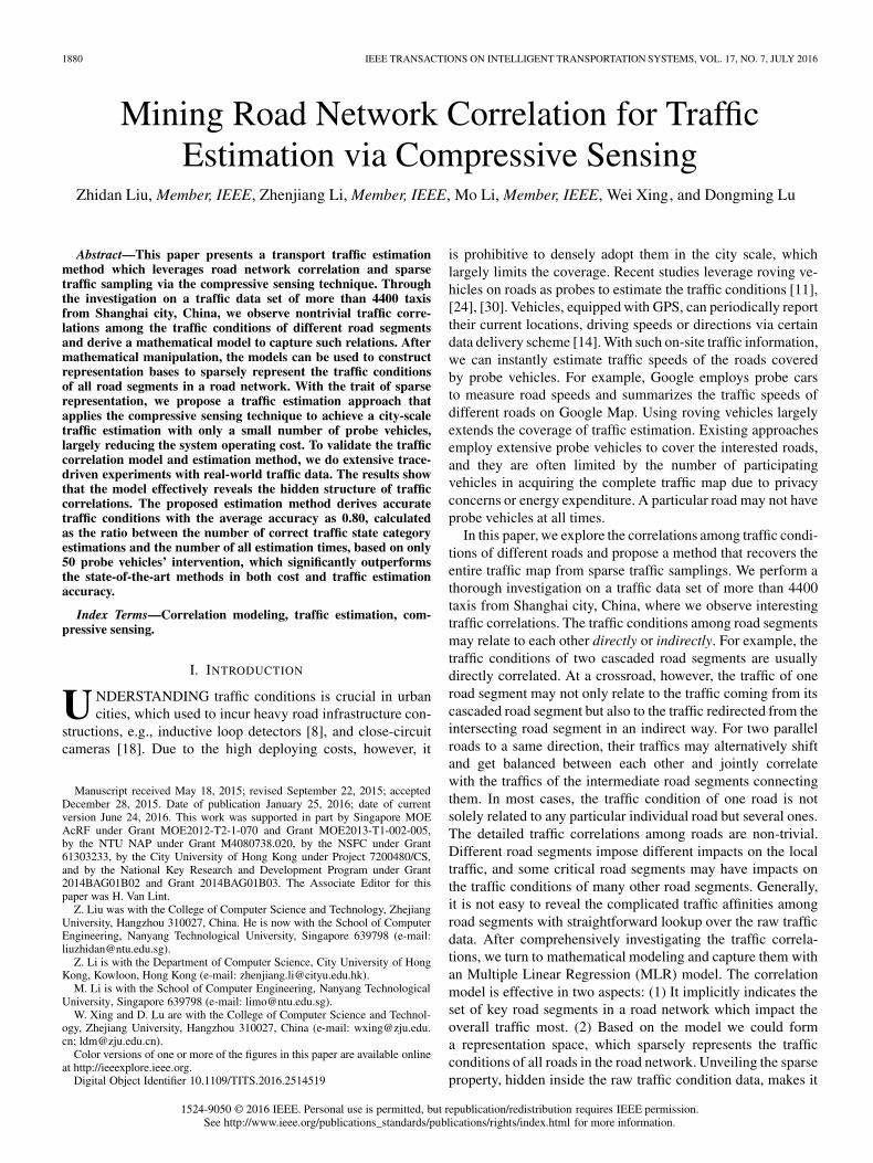
We test the traffic sparsity with the 4th-week traffic data.For each time frame, we can obtain a congestion rate vector c.According to which traffic scenario the time frame belongsto, we calculate s = Pc with the corresponding representationmatrix, and examine the sparsity of s. Different MLR modelsof road segments in different traffic scenarios lead to differentP in Eq. (4), and thus different Ψ. We find that s is of goodsparsity in all four traffic scenarios as shown in Fig. 7. With athreshold 0.01, the sparsity in any traffic scenario is less than25 that is much smaller than the total number of road segments


Fig. 7. The sparsity of representation s in domain Ψ for the four trafficscenarios.

386. As a result, the representation matrixP , constructed by ourtraffic models, can sparsely describe the traffic conditions. Wethus obtain a set of suitable representation bases Ψ = P−1 forall the four traffic scenarios, which can be used in compressivesensing technique to recover c.

Computation Complexity: If a road network consists of nroad segments and we correlate the traffic condition of eachroad segment with all other n− 1 road segments, the com-putation complexity to mine traffic correlations using MLR isO(n3W ), where W is the total number of training examples.With the coefficient pruning, however, the computation com-plexity can be significantly reduced to O(κ2nW ), where κ is asmall constant defined in the “Coefficient pruning” subsectionand κ � n. We will further investigate the MLR computationcomplexity experimentally in Section V-E, which shows that ittakes only several minutes to establish our MLR model for alarge road network with thousands of road segments.

B. Traffic Estimation via Compressive Sensing

We have constructed the representation bases Ψ for the trafficestimation problem Y = ΦΨs+ e. In this subsection, we willintroduce how to obtain the measurement vector Y and themeasurement matrix Φ using a small number of probe vehicles,and then obtain the timely traffic condition estimation of allroad segments via a compressive sensing solver.

Measurement Vector Y : A server continuously collects traf-fic samplings from a fleet of probe vehicles in each time frameand estimates the global traffic conditions at the end of the timeframe. In other words, the size of time frame is the time granu-larity of traffic estimation. A smaller time frame leads to moretimely updating of traffic states. In any time frame, supposethe server collects samplings from m probe vehicles, h1 to hm.According to the time stamps contained in the traffic samplings,we get their traveling times, and for each probe vehicle hj ,we denote thj

as its traveling time. Y = [th1, th2

, . . . , thm]T

is thus the measurement vector in the compressive sensingformulation.

Measurement Matrix Φ: Based on the GPS positions re-ported by each probe vehicle, we can calculate their traveling

trajectories on the road map. To overcome the noise of GPSdata, we adopt an Hidden Markov Model (HMM) based mapmatching algorithm [17] to match a sequence of GPS positionssparsely sampled by one probe vehicle to the most likelysequence of road segments. By viewing actually travelled roadsegments as hidden states and traffic samplings as observations,[17] has shown that the HMM based map matching methodachieves high mapping accuracy and efficiency. Thus, we usethe output of HMM based map matching method as the finalvehicle trajectory. Specifically, for probe vehicle hj , we canconstruct a vector Lhj

= {lrihj, i = 1, 3, . . . , n} according to its

trajectory. Each lrihjin Lhj

indicates the distance hj travels onthe road segment ri, which can be calculated as:

lrihj=

{drihj

, ri is passed by hj

0, otherwise

where drihjis the actual traveled distance by probe vehicle hj

on road segment ri. If ri is fully covered by the trajectory ofhj , then drihj

is the length of ri; otherwise, the traveled distanceis computed as the great circle distance via an map matchingtechnique. Based on each Lhj

, we can construct an m× nmatrix as [Lh1

;Lh2; . . . ;Lhm

]T . Considering the constant itemβri,0 in MLR model, we add a zero value at the first position ofeach distance vector, and obtain the final m× (n+ 1) matrixas Eq. (5) that is the measurement matrix Φ for the compressivesensing formulation. Since each probe vehicle travels freely inthe city, the trajectories of any two vehicles are independent [2].As a result, the measurement matrix Φ constructed in Eq. (5)is a random matrix, which satisfies the requirement by compres-sive sensing on Φ, whose elements should be randomly chosen.

Φ =

⎡⎢⎢⎢⎣

0 lr1h1lr2h1

· · · lrnh1

0 lr1h2lr2h2

· · · lrnh2

......

.... . .

...0 lr1hm

lr2hm· · · lrnhm

⎤⎥⎥⎥⎦ . (5)

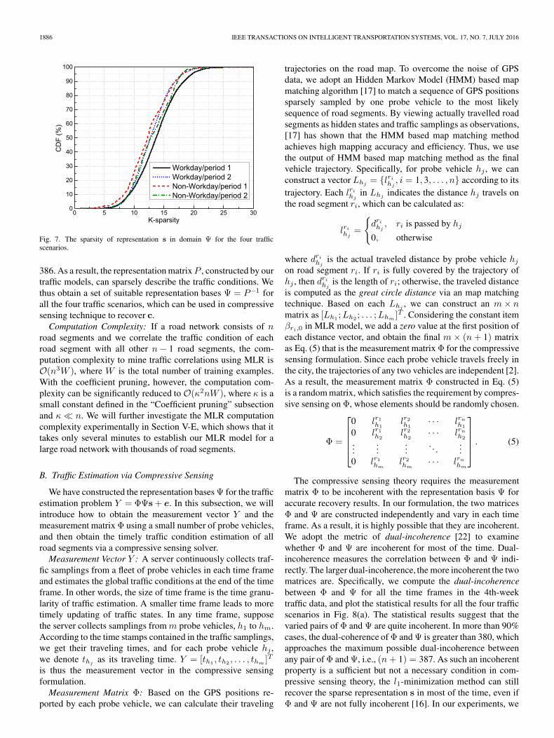
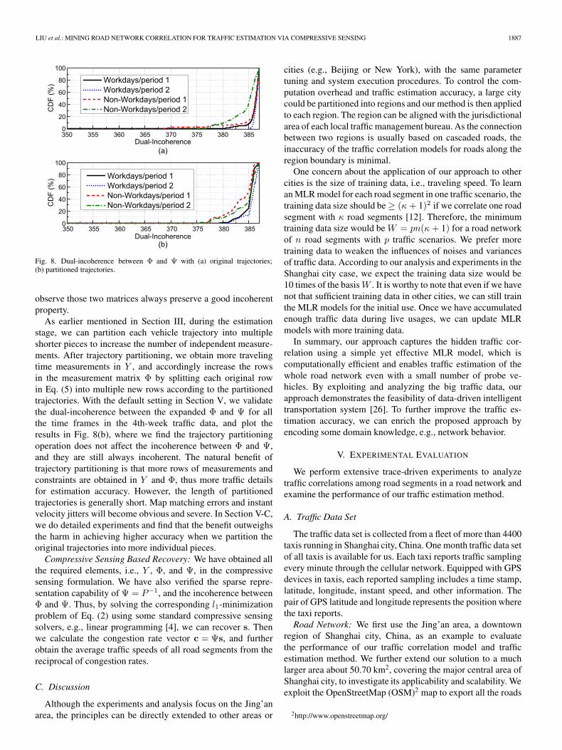
The compressive sensing theory requires the measurementmatrix Φ to be incoherent with the representation basis Ψ foraccurate recovery results. In our formulation, the two matricesΦ and Ψ are constructed independently and vary in each timeframe. As a result, it is highly possible that they are incoherent.We adopt the metric of dual-incoherence [22] to examinewhether Φ and Ψ are incoherent for most of the time. Dual-incoherence measures the correlation between Φ and Ψ indi-rectly. The larger dual-incoherence, the more incoherent the twomatrices are. Specifically, we compute the dual-incoherencebetween Φ and Ψ for all the time frames in the 4th-weektraffic data, and plot the statistical results for all the four trafficscenarios in Fig. 8(a). The statistical results suggest that thevaried pairs of Φ and Ψ are quite incoherent. In more than 90%cases, the dual-coherence of Φ and Ψ is greater than 380, whichapproaches the maximum possible dual-incoherence betweenany pair of Φ and Ψ, i.e., (n+ 1) = 387. As such an incoherentproperty is a sufficient but not a necessary condition in com-pressive sensing theory, the l1-minimization method can stillrecover the sparse representation s in most of the time, even ifΦ and Ψ are not fully incoherent [16]. In our experiments, we


Fig. 8. Dual-incoherence between Φ and Ψ with (a) original trajectories;(b) partitioned trajectories.

observe those two matrices always preserve a good incoherentproperty.

As earlier mentioned in Section III, during the estimationstage, we can partition each vehicle trajectory into multipleshorter pieces to increase the number of independent measure-ments. After trajectory partitioning, we obtain more travelingtime measurements in Y , and accordingly increase the rowsin the measurement matrix Φ by splitting each original rowin Eq. (5) into multiple new rows according to the partitionedtrajectories. With the default setting in Section V, we validatethe dual-incoherence between the expanded Φ and Ψ for allthe time frames in the 4th-week traffic data, and plot theresults in Fig. 8(b), where we find the trajectory partitioningoperation does not affect the incoherence between Φ and Ψ,and they are still always incoherent. The natural benefit oftrajectory partitioning is that more rows of measurements andconstraints are obtained in Y and Φ, thus more traffic detailsfor estimation accuracy. However, the length of partitionedtrajectories is generally short. Map matching errors and instantvelocity jitters will become obvious and severe. In Section V-C,we do detailed experiments and find that the benefit outweighsthe harm in achieving higher accuracy when we partition theoriginal trajectories into more individual pieces.

Compressive Sensing Based Recovery: We have obtained allthe required elements, i.e., Y , Φ, and Ψ, in the compressivesensing formulation. We have also verified the sparse repre-sentation capability of Ψ = P−1, and the incoherence betweenΦ and Ψ. Thus, by solving the corresponding l1-minimizationproblem of Eq. (2) using some standard compressive sensingsolvers, e.g., linear programming [4], we can recover s. Thenwe calculate the congestion rate vector c = Ψs, and furtherobtain the average traffic speeds of all road segments from thereciprocal of congestion rates.

C. Discussion

Although the experiments and analysis focus on the Jing’anarea, the principles can be directly extended to other areas or

cities (e.g., Beijing or New York), with the same parametertuning and system execution procedures. To control the com-putation overhead and traffic estimation accuracy, a large citycould be partitioned into regions and our method is then appliedto each region. The region can be aligned with the jurisdictionalarea of each local traffic management bureau. As the connectionbetween two regions is usually based on cascaded roads, theinaccuracy of the traffic correlation models for roads along theregion boundary is minimal.

One concern about the application of our approach to othercities is the size of training data, i.e., traveling speed. To learnan MLR model for each road segment in one traffic scenario, thetraining data size should be ≥ (κ+ 1)2 if we correlate one roadsegment with κ road segments [12]. Therefore, the minimumtraining data size would be W = pn(κ+ 1) for a road networkof n road segments with p traffic scenarios. We prefer moretraining data to weaken the influences of noises and variancesof traffic data. According to our analysis and experiments in theShanghai city case, we expect the training data size would be10 times of the basis W . It is worthy to note that even if we havenot that sufficient training data in other cities, we can still trainthe MLR models for the initial use. Once we have accumulatedenough traffic data during live usages, we can update MLRmodels with more training data.

In summary, our approach captures the hidden traffic cor-relation using a simple yet effective MLR model, which iscomputationally efficient and enables traffic estimation of thewhole road network even with a small number of probe ve-hicles. By exploiting and analyzing the big traffic data, ourapproach demonstrates the feasibility of data-driven intelligenttransportation system [26]. To further improve the traffic es-timation accuracy, we can enrich the proposed approach byencoding some domain knowledge, e.g., network behavior.

V. EXPERIMENTAL EVALUATION

We perform extensive trace-driven experiments to analyzetraffic correlations among road segments in a road network andexamine the performance of our traffic estimation method.

A. Traffic Data Set

The traffic data set is collected from a fleet of more than 4400taxis running in Shanghai city, China. One month traffic data setof all taxis is available for us. Each taxi reports traffic samplingevery minute through the cellular network. Equipped with GPSdevices in taxis, each reported sampling includes a time stamp,latitude, longitude, instant speed, and other information. Thepair of GPS latitude and longitude represents the position wherethe taxi reports.

Road Network: We first use the Jing’an area, a downtownregion of Shanghai city, China, as an example to evaluatethe performance of our traffic correlation model and trafficestimation method. We further extend our solution to a muchlarger area about 50.70 km2, covering the major central area ofShanghai city, to investigate its applicability and scalability. Weexploit the OpenStreetMap (OSM)2 map to export all the roads

2http://www.openstreetmap.org/

http://www.openstreetmap.org/


in those areas, and segment the roads according to their inter-secting points. In OSM map, two driving directions of the roadsare represented separately. The trajectory of each vehicle couldbe mapped to the corresponding directional road segments. Weclassify the geographic structure of all road segments into threegroups: “cascaded,” “intersected,” and “apart.” “Cascaded”includes road segments connected with the same road name,while “intersected” contains connected road segments withdifferent road names. OSM contains 926 road segments totallyin the Jing’an area and we select a subset of 386 road segmentswith sufficient coverage by the taxi data, which form a roadnetwork for our experiments. We refer to road attributes andfind that the selected 386 roads completely cover all primaryand secondary roads in this area. Similarly, we select 1826out of totally 3451 road segments from the central area withsufficient taxi data coverage. Note that road segment selectionaims to obtain the ground truth for the performance evaluationonly. In practice, after the traffic models are constructed, ourmethod can estimate the traffic conditions for the whole roadnetwork. Throughout the one month traffic data, the numberof probe taxis within the Jing’an area (central area) rangesfrom 65 to 498 (175 to 906) in each time frame. As probevehicles travel along road segments freely in a road network,we thus use the traffic samplings from randomly selected taxisfor the traffic estimation to best match the real scenario. Bydefault, we use the traffic samplings from 50 randomly taxis forthe traffic estimation in each time frame. Probe taxis generateadequate traffic data for both model training and performancetesting, e.g., we have about 5 millions traffic samplings forthe Jing’an area and about 14 millions traffic samplings forShanghai central area.

Traffic Data Preprocessing: We divide the one month trafficdata for each 15 min time frame and classify into four trafficscenarios as described in Section IV-A. Time frames with sizeof 15 min are long enough to accumulate sufficient trafficsamplings for accurate map matching for each probe taxi, andalso provide a fine granularity for timely traffic estimation[13], [23], [30]. By default, we use the data of all taxis inthe first three weeks to train the MLR models and the data ofa small subset of those taxis in the last week to evaluate theperformance of our approach. In each time frame, we calculatethe average traffic speed of each road segment as the averagevalue of all reported speeds by all taxis passing by. In casethere is no reported speeds for a road segment in one timeframe, we use the average speed of this road segment in theprevious 4 time frames. After the traffic data preprocessing,every road segment has a speed in each time frame, and thus thecongestion rate. Those average speeds are treated as the pseudoground truth, and used to evaluate the performance of our trafficestimation method.

B. Traffic Correlation Analysis

To train MLR models for each road segment ri, ri selects itstop κ correlated segments from the rest n− 1 road segments.κ is set to 10 according to the prior empirical investigationin Fig. 6. We first study the geography distribution of the topcorrelated road segments derived from our traffic models. The

Fig. 9. (a) CDF of distance between top correlated road segments. (b) Statisti-cal results of correlation types in the four traffic scenarios.

physical distance distribution of pair-wise correlated road seg-ments is plotted in Fig. 9(a). We find that 90% correlated roadsegments locate within the range of 0.5 km, where the distancebetween two road segments is measured from their midpoints.For each road segment, correlated segments are mainly from itsvicinity giving good locality in traffic correlation. On the otherhand, we further examine the logic relationship between eachroad segment and its κ correlated road segments. We observe774 cascaded pairs (20%), 1711 intersected pairs (44%), and1375 apart pairs (36%). As “cascaded” and “intersected” ac-count for 64% in total, it implies that around 26% of “apart”pairs also preserve the correlation locality (e.g., the “parallel”case). In addition, remote segments (> 0.5 km) contribute non-negligible portions as well, e.g., 10%. Above correlations arehidden and largely omitted in previous works, e.g., [13], [23],[29], [30]. They cannot be unveiled unless with an explicitlyderived traffic model.

We then investigate how each road segment ri is related toother road segments by examining the normalized regressioncoefficients in the MLR model. If there is a dominant coeffi-cient, ri is viewed as directly correlated with that particular roadsegment. Otherwise, ri is indirectly correlated with a set of roadsegments. We empirically select 0.35 as the threshold to find thedominant coefficient for road segment ri. We believe 0.35 isgreat enough to filter the most predominant road segment fromthe κ = 10 correlated road segments of ri. Fig. 9(b) depicts thedistributions of correlation types in all the four traffic scenar-ios. Although the percentage of direct correlation is high, inaround half of the cases, road segments are indirectly correlatedwith other segments. The results imply that plenty of implicitcorrelations are hidden among different road segments. Suchcorrelations are not directly visible unless explored by a methodsuch as the proposed traffic model.

C. Basic Evaluation

Trajectory Separation: We conduct experiments to explore theimpacts of trajectory partitioning, and show its effectiveness.


Fig. 10. Average absolute speed differences between pseudo ground truths andestimated speeds with various partitioned pieces of each trajectory.

A trajectory generally can be partitioned into multiple piecesaccording to the amount of traffic samplings. For the originaltrajectories of randomly selected probe taxis, we uniformlypartition each of them into x pieces and perform trafficestimation based on the partitioned trajectories. Fig. 10 plotsthe average absolute speed differences between the pseudoground truths and estimated speeds when we partition eachoriginal trajectory into x pieces of short trajectories (ifpossible), where x = 1 means we perform the traffic estimationwith the original trajectories. From Fig. 10, we find that wheneach original trajectory is partitioned into more pieces, theaverage absolute speed difference tends to be smaller. Theseresults imply that benefits outweighs the harm in achievinghigher traffic estimation accuracy. According to the experiment,we obtain better estimation results when we partition eachoriginal trajectory into maximum possible number (15 pieces ineach 15 min time frame) of short trajectories. We see negligibleperformance gain beyond x = 10 pieces of partition, and weuse this as the default setting for all following experiments.

Traffic Estimation Accuracy: We first show a snapshot ofestimated traffic speeds of all road segments in one randomlyselected time frame in Fig. 11. This figure shows that the esti-mated speeds cross different road segments match the trend ofthe pseudo ground truths very well. To quantify the differencebetween the pseudo ground truths and the estimated speeds,we plot the CDF of absolute speed differences between themover the four traffic scenarios across the entire 4th-week trafficdata in Fig. 12(a). Due to the inherently higher traffic dynamicsin workdays, e.g., the high taxi velocity fluctuation and trafficvariance due to traffic jams in workdays, the performancein non-workdays is generally better. The 90-percentile and60-percentile speed differences are 10.5 km/h and 5.2 km/hfor non-workdays and 11.0 km/h and 5.6 km/h for workdaysrespectively. In general, the estimated speed for each roadsegment is in good accuracy but always slightly smaller than itspseudo ground truth with overall difference less than 5.0 km/h.It is because in the measurement vector Y , the time differencebetween the last and the first samplings within a time frame maycontain certain time that should not be included, e.g., the waiting

Fig. 11. The traffic estimation snapshot of a randomly selected time frame,with comparison of the pseudo ground truths.

Fig. 12. CDF of (a) the absolute speed differences; (b) the estimation accuracywith respect to four different traffic condition indicators.

time for traffic lights. The measured traveling time is thusgreater than the actual one and thus a smaller estimated speed.

Instead of directly giving the speed estimations, we translatethe estimated speed to a more meaningful traffic indicator foreach road. It is worthy to note that different from previousmethods only providing coarse traffic levels [9], [23], ourmethod can provide the detailed traveling speed information foreach road segment. Similar with Google Map, we classify thetraffic conditions of each road segment ri to four categoriesaccording to its traffic speed vi (in km/h), i.e., Congested(vi < 20), Slow (20 ≤ vi < 40), Normal (40 ≤ vi < 60) andFast (vi ≥ 60). We then compute the estimation accuracy as(# of estimation hits/# of total time frames), where an esti-mation hit means both the pseudo ground truth and the esti-mated speed are classified to a same category in one time frame.From the results in Fig. 12(b), We find that the four trafficscenarios have similar estimation accuracy distribution, whichconcentrates within a high accuracy range between 0.75 and0.90. The accuracy achieves up to 0.94 and the overall average


Fig. 13. (a) Estimation accuracy with different numbers of probe taxis used;(b) Estimation accuracy with different number of weeks training data.

is more than 0.80, which provides quite accurate estimationresults.

Number of Probe Vehicles: In this experiment, we investi-gate the impact of the probe taxi number on the estimationperformance of our method. We vary the taxi number used inthe traffic estimation (denoted as m) from 10 to 300, and plotthe estimation accuracy in Fig. 13(a). Since probe vehicles inpractice travel independently in a road network, m taxis areselected randomly in each time frame to best match the reality.If the total amount of taxis in the road network is smallerthan m (e.g., in the early morning), we use all available taxisfor the traffic estimation. From the figure, we find when mis very small (e.g., 10 or 20), the estimation already achieveshigh accuracy on average (> 0.70), but with a large variance.After the number of taxis used is greater than 50, the averageestimation accuracy stabilizes around 0.80 while the standarddeviation continuously decreases as more taxis are used in theestimation. Based on the statistics, we find that the accuracyimprovement and standard deviation reduction are only 1.54%and 19.16% respectively, when the taxis number increases from50 to 300. With our method, a small group of probe taxis canoffer comparable accuracy as that from a large number of probetaxis. Hence, our default setting m = 50 leads to both goodestimation performance and low system operation cost.

Training Data Size: We vary the training data size fromone week to three weeks and use a small subset of data ofthe subsequent week from 50 probes as the testing data toinvestigate the impacts of training data size. Fig. 13(b) plotsthe estimation accuracy, where we find more training data canlead to higher accuracy, which is attributed to the better trainedMLR models. On the other hand, we also find that even moredata may bring slight improvement. For example, when weincrease the training data size from two weeks to three weeks,the accuracy improvement is only 0.02. It is worthy to note thateven with one week training data our method can achieve highaccuracy as 0.72. This implies that our method can work welleven with a small set of initial training data.

Fig. 14. (a) Road network coverage by different methods; (b) Estimationaccuracy of road segments directly covered by taxis with different methods.

D. Performance Comparison

We compare our traffic estimation method with a baselinemethod and the state-of-the-art method SVD-TE [13], [30].

With Baseline Method: Within a time frame, traffic condi-tions of the road segments, on which one or more taxis reporttraffic samplings, can also be measured by the average of instantspeeds in traffic samplings, we name such a method as the base-line method. Since sparse taxis partially cover a road networkin each time frame, baseline method provides an alternativeway to obtain traffic conditions of those road segments directlycovered by probe taxis only. With sparse probe taxis (i.e.,50 taxis), Fig. 14(a) shows that such naive method covers lessthan 45% road segments of the road network in all the fourtraffic scenarios, while our method can always estimate thetraffic conditions of the whole road network. In Fig. 14(b),we compare their estimation accuracies. For a fair comparison,in each time frame, we compare the estimation accuracy onlyon the road segments with reported traffic samplings [with thesame metric as Fig. 12(b)]. Due to high variance of each instantspeed, the accuracy of the baseline method is only around 0.66.Our method achieves an accuracy around 0.80 in all the fourscenarios and outperforms the baseline method by 17.13%. Thisis because our method uses traveling time and distance of taxitrajectories to estimate the average traveling speed of each roadsegment, which avoids the biased speed observations in trafficsamplings due to dynamic taxi behaviors.

With State-of-the-Art Method: SVD-TE utilizes the spatialtemporal correlation in traffic matrix constructed by recent traf-fic samplings to recover missing elements. Specifically, SVD-TE accumulates traffic samplings in an n× t traffic matrixand then leverages the singular value decomposition (SVD)technique to recover the missing traffic conditions in the trafficmatrix. n is fixed as the total number of road segments in aroad network, and t can be varying which determines a windowsize to accommodate traffic conditions in the SVD recovery.Fig. 15(a) shows that the estimation accuracy of SVD-TE is lowwhen the matrix width (i.e., t) is small and stabilizes around


Fig. 15. (a) Estimation accuracy of SVD-TE with various matrix width t;(b) Comparison on estimation accuracy of our method and SVD-TE.

0.63 when it is greater than 32 time frames (i.e., 480 minutes).In Fig. 15(b), we compare our method with SVD-TE when tadopts 32. Our method outperforms SVD-TE on the estimationaccuracy about 20%. In addition, our method can estimatetraffic conditions of the entire road network every 15 minutes(i.e., one time frame). Such a short delay is necessary in practicedue to the timeliness of traffic estimation. The major differencebetween our work and SVD-TE is that we have explicitly builtthe traffic correlation model and thus strengthened efficiency ofcompressive sensing technique, to which the great advantagesof our method are attributed.

E. Scalability Evaluation

We evaluate our method in a larger road network to under-stand its applicability and scalability in practice. The networkdetails have been introduced in Section V-A. To control thecomputation overhead, a large area could be partitioned intoseveral regions and our method is then applied to each region,just as described in Section IV-C. The large road network in thisexperiment trial is divided into 4 regions, A, B, C, and D. Eachregion is slightly larger than the Jing’an area.

Computation Overhead: We will first investigate the compu-tation overhead. We apply our method to four road networks A,A ∪ B, A ∪ B ∪ C, and A∪ B ∪ C ∪ D, with different scales,where the union of multiple regions means regions togetherform a road network. All experiments in this section areconducted on a desktop with quad-core 2.66Ghz CPU and4GB RAM, and we use the program execution time as theperformance metric to evaluate the computation overhead. Twophases of our method may incur high computation overhead:MLR modeling and compressive sensing recovery, and resultsare detailed in Fig. 16. In a single region, e.g., A with 451road segments, the construction of the MLR models can befinished within one minute. As the network scales, the MLRconstruction overhead linearly increases. However, the MLRmodel construction is infrequent and offline in our method, e.g.,

Fig. 16. Execution time of (a) the construction of MLR models; (b) compres-sive sensing recovery with reports from 50 taxis within one time frame.

Fig. 17. Estimation accuracy in the large road network with 50.70 km2

coverage when our method is applied using region partition and directly.

the MLR model could be updated every one or two months,the computation overhead is still practically acceptable, e.g.,less than 8 minutes for a road network covering 50.7 km2.If the region partition mechanism is used, the MLR modelconstruction in each region can be parallel, which leads toa significant improvement, e.g., overall less than 1 minuteoverhead. On the other hand, Fig. 16(b) further indicates thatthe overhead due to compressive sensing recovery is negligiblewhich is less than 0.3 seconds with traffic samplings from50 randomly selected taxis within each 15 min time frame.

Estimation Accuracy: We finally examine the estimationaccuracy of our method using the region partition mechanismon the large road network with 50.70 km2 coverage, denotedas “Partitioned” in Fig. 17. As a benchmark, we also plot theperformance when directly applying our method to the wholenetwork, denoted as “Original.” Fig. 17 shows that “Parti-tioned” achieves comparable accuracy with “Original” in bothworkdays and non-workdays. Both Figs. 16 and 17 validate theapplicability and scalability of our method.


VI. CONCLUSION AND FUTURE WORK

This paper presents a transport traffic estimation methodwhich applies compressive sensing technique to achieve city-scale traffic estimation with only sparse traffic probes. Thestrong correlations among the road network is captured byan explicit model and further exploited to form a space basisthat can sparsely represent the road traffic conditions. Throughextensive trace-driven study and experiments, we validate theeffectiveness of our traffic correlation model and show that ourapproach achieves accurate and scalable traffic estimation withonly sparse probes.

As future works, we plan to remove the traffic estimationbias due to the inaccurate traveling time calculated from trafficdata. It is also of interest to encode some transportation domainknowledge, e.g., routing behavior and network equilibrium, intoour approach to further improve the estimation accuracy.

REFERENCES

[1] M. Abdel-Aty and A. Pande, “ATMS implementation system for identi-fying traffic conditions leading to potential crashes,” IEEE Trans. Intell.Transp. Syst., vol. 7, no. 1, pp. 78–91, Mar. 2006.

[2] J. Aslam, S. Lim, X. Pan, and D. Rus, “City-scale traffic estimation froma roving sensor network,” in Proc. ACM SenSys, 2012, pp. 141–154.

[3] E. J. Candès, J. Romberg, and T. Tao, “Robust uncertainty principles: Ex-act signal reconstruction from highly incomplete frequency information,”IEEE Trans. Inf. Theory, vol. 52, no. 2, pp. 489–509, Feb. 2006.

[4] E. J. Candès and T. Tao, “Decoding by linear programming,” IEEE Trans.Inf. Theory, vol. 51, no. 12, pp. 4203–4215, Dec. 2005.

[5] C. Chen et al., “Tripplanner: Personalized trip planning leveraging het-erogeneous crowdsourced digital footprints,” IEEE Trans. Intell. Transp.Syst., vol. 16, no. 3, pp. 1259–1273, Jun. 2015.

[6] D. L. Donoho, “Compressed sensing,” IEEE Trans. Inf. Theory, vol. 52,no. 4, pp. 1289–1306, Apr. 2006.

[7] D. L. Donoho, M. Elad, and V. N. Temlyakov, “Stable recovery of sparseovercomplete representations in the presence of noise,” IEEE Trans. Inf.Theory, vol. 52, no. 1, pp. 6–18, Jan. 2006.

[8] J. Han, J. W. Polak, J. Barria, and R. Krishnan, “On the estimation ofspace-mean-speed from inductive loop detector data,” Transp. Plann.Technol., vol. 33, no. 1, pp. 91–104, Feb. 2010.

[9] R. Herring, A. Hofleitner, P. Abbeel, and A. Bayen, “Estimating arterialtraffic conditions using sparse probe data,” in Proc. IEEE ITSC, 2010,pp. 929–936.

[10] E. Horvitz, J. Apacible, R. Sarin, and L. Liao, “Prediction, expectation,and surprise: Methods, designs, and study of a deployed traffic forecastingservice,” in Proc. UAI, 2005, pp. 275–280.

[11] T. Idé and M. Sugiyama, “Trajectory regression on road networks,” inProc. AAAI, 2011, pp. 203–208.

[12] M. H. Kutner, C. Nachtsheim, and J. Neter, Applied Linear RegressionModels. New York, NY, USA: McGraw-Hill, 2004.

[13] Z. Li, Y. Zhu, H. Zhu, and M. Li, “Compressive sensing approach to urbantraffic sensing,” in Proc. IEEE ICDCS, 2011, pp. 889–898.

[14] Y. Liu, Z. Yang, T. Ning, and H. Wu, “Efficient quality-of-service (QoS)support in mobile opportunistic networks,” IEEE Trans. Veh. Technol.,vol. 63, no. 9, pp. 4574–4584, Nov. 2014.

[15] Y. Lv, Y. Duan, W. Kang, Z. Li, and F.-Y. Wang, “Traffic flow predictionwith big data: A deep learning approach,” IEEE Trans. Intell. Transp.Syst., vol. 16, no. 2, pp. 865–873, Apr. 2015.

[16] P. Misra, W. Hu, M. Yang, and S. Jha, “Efficient cross-correlation viasparse representation in sensor networks,” in Proc. ACM/IEEE IPSN,2012, pp. 13–24.

[17] P. Newson and J. Krumm, “Hidden Markov map matching through noiseand sparseness,” in Proc. ACM GIS, 2009, pp. 336–343.

[18] T. N. Schoepflin and D. J. Dailey, “Dynamic camera calibration of road-side traffic management cameras for vehicle speed estimation,” IEEETrans. Intell. Transp. Syst., vol. 4, no. 2, pp. 90–98, Jun. 2003.

[19] R. Sen et al., “Kyun queue: A sensor network system to monitor roadtraffic queues,” in Proc. ACM SenSys, 2012, pp. 127–140.

[20] Y. Wang, Y. Zheng, and Y. Xue, “Travel time estimation of a path usingsparse trajectories,” in Proc. ACM SIGKDD, 2014, pp. 25–34.

[21] Y. Wang, Y. Zhu, Z. He, Y. Yue, and Q. Li, “Challenges and opportunitiesin exploiting large-scale GPS probe data,” HP Labs, Palo Alto, CA, USA,HP Tech. Rep. HPL-2011-109, 2011.

[22] X. Wu and M. Liu, “In-situ soil moisture sensing: Measurement schedul-ing and estimation using compressive sensing,” in Proc. ACM/IEEE IPSN,2012, pp. 1–11.

[23] B. Yang, C. Guo, and C. S. Jensen, “Travel cost inference from sparse,spatio temporally correlated time series using Markov models,” in Proc.VLDB, 2013, pp. 769–780.

[24] B. Yang, M. Kaul, and C. S. Jensen, “Using incomplete information forcomplete weight annotation of road networks,” IEEE Trans. Knowl. DataEng., vol. 26, no. 5, pp. 1267–1279, May 2014.

[25] J. Yoon, B. Noble, and M. Liu, “Surface street traffic estimation,” in Proc.ACM MobiSys, 2007, pp. 220–232.

[26] J. Zhang et al., “Data-driven intelligent transportation systems: A sur-vey,” IEEE Trans. Intell. Transp. Syst., vol. 12, no. 4, pp. 1624–1639,Dec. 2011.

[27] J. Zheng and L. M. Ni, “Time-dependent trajectory regression on road net-works via multi-task learning,” in Proc. AAAI, 2013, pp. 1048–1055.

[28] P. Zhou, Y. Zheng, and M. Li, “How long to wait?: Predicting bus ar-rival time with mobile phone based participatory sensing,” in Proc. ACMMobiSys, 2012, pp. 379–392.

[29] H. Zhu, Y. Zhu, M. Li, and L. M. Ni, “SEER: Metropolitan-scale trafficperception based on lossy sensory data,” in Proc. IEEE INFOCOM, 2009,pp. 217–225.

[30] Y. Zhu, Z. Li, H. Zhu, M. Li, and Q. Zhang, “A compressive sensingapproach to urban traffic estimation with probe vehicles,” IEEE Trans.Mobile Comput., vol. 12, no. 11, pp. 2289–2302, Nov. 2013.

Zhidan Liu (M’15) received the B.E. degree incomputer science and technology from NortheasternUniversity, Shenyang, China, in 2009 and the Ph.D.degree in computer science and technology fromZhejiang University, Hangzhou, China, in 2014. Heis currently a Research Fellow at Nanyang Techno-logical University, Singapore. His research interestsinclude wireless sensor networks, mobile computing,and big data analytics.

Zhenjiang Li (M’12) received the B.E. degreein computer science and technology from Xi’anJiaotong University, Xi’an, China, in 2007 and theM.Phil. degree in electronic and computer engineer-ing and the Ph.D. degree in computer science andengineering from The Hong Kong University of Sci-ence and Technology, Hong Kong, in 2009 and 2012,respectively. He is currently an Assistant Professorof computer science at City University of HongKong, Hong Kong. His research interests includemobile sensing and computing, wireless networks,

and distributed networking systems.

Mo Li (M’06) received the B.S. degree in computerscience and technology from Tsinghua University,Beijing, China, in 2004 and the Ph.D. degree in com-puter science and engineering from The Hong KongUniversity of Science and Technology, Hong Kong,in 2009. He is currently an Assistant Professorwith the School of Computer Engineering, NanyangTechnological University, Singapore. His researchinterests include wireless sensor networks, pervasivecomputing, and mobile and wireless computing.


Wei Xing received the B.E., M.E., and Ph.D. de-grees from Zhejiang University, Hangzhou, China,in 1989, 1992, and 2009, respectively. In 1992, hejoined the Department of Control, College of In-formation Technology, Zhejiang University. Since2002, he has been with the College of ComputerScience and Technology, Zhejiang University, wherehe is currently an Associate Professor. His researchinterests include multimedia technology and Internetof Things.

Dongming Lu received the B.E., M.E., and Ph.D.degrees from Zhejiang University, Hangzhou, China,in 1989, 1991, and 1994, respectively. He is currentlya Professor with the College of Computer Scienceand Technology, Zhejiang University. His researchinterests include Internet of Things, multimedia tech-nology, and digital preservation of cultural heritage.

Mining Road Network Correlation for Trafﬁc Estimation ... · Mining Road Network Correlation for...

Documents

Transcript of Mining Road Network Correlation for Trafﬁc Estimation ... · Mining Road Network Correlation for...