Mining and Querying Multimedia Data

Mining and Querying Multimedia Data

Fan Guo

CMU-CS-11-133

September 29, 2011

School of Computer ScienceCarnegie Mellon University

Pittsburgh, PA 15213

Thesis Committee:Christos Faloutsos, Chair

Eric P. XingWilliam W. Cohen

Ambuj K. Singh, University of California at Santa Barbara

Submitted in partial fulfillment of the requirementsfor the degree of Doctor of Philosophy.

Copyright c© 2011 Fan Guo

This research was sponsored by the National Science Foundation under grant numbers DBI-0546594, DBI-0640543,and IIS-0970179, NRO under grand number 000-09-C-0150, andthe Army Research Laboratory under grant numberW911NF-09-2-0053. The views and conclusions contained in this document are those of the author and should notbe interpreted as representing the official policies, either expressed or implied, of any sponsoring institution, theU.S. government or any other entity.

Keywords: data mining, graph mining, Web search

To my parents

AbstractThe emerging popularity of multimedia data, as digital representation of text,

image, video and countless other milieus, with prodigious volumes and wild diver-sity, exhibits the phenomenal impact of modern technologies in reforming the wayinformation is accessed, disseminated, digested and retained. This has iterativelyignited the data-driven perspective of research and development, to characterize per-spicuous patterns, crystallize informative insights, andrealize elevated experiencefor end-users, where innovations in a spectrum of areas of computer science, in-cluding databases, distributed systems, machine learning, vision, speech and naturallanguages, has been incessantly absorbed and integrated toelicit the extent and effi-cacy of contemporary and future multimedia applications and solutions.

Under the theme of pattern mining and similarity querying, this manuscriptpresents a number of pieces of research concerning multimedia data, to addressan array of practical tasks encompassing automatic annotation, outlier detection,community discovery, multi-modal retrieval and learning to rank, in their respectivecontexts including satellite image analysis, internet traffic surveillance, image bioin-formatics, and Web search. A repertoire of extant and novel techniques pertaining tograph mining, clustering analysis, tensor decomposition and probabilistic graphicalmodels has been developed or adapted, which satisfactorilymet differing quality andefficiency requisites postulated by specific application settings, best exemplified bythe 40 times speed-up in annotating satellite images and theup to 30% performanceimprovement in predicting web search user clicks, yet without the loss of generalityto similar and related scenarios.

AcknowledgmentsThis manuscript would never be completed without the inspiration, support, trust

and humor from my advisor, Christos Faloutsos, to whom I owe the greatest grati-tude for the gaiety of graduate study. I’d like to thank Professor Eric Xing for hismentorship that matured my minds on research, Professor William Cohen for hiscareful review of the thesis and proposal drafts, and Professor Ambuj Singh for hisinsightful questions and comments.

I’m honored to be a member of the database group, with Jia-Yu Pan, IppokratisPandis, Jimeng Sun, Debabrata Dash, Jure Leskovec, Hanghang Tong, Mary Mc-Glohon, Lei Li, Leman Akoglu, Polo Chau, B. Aditya Prakash, UKang, and DanaeKoutra, and enjoying the collaboration with our visitors and colleagues residing onseveral continents – Michael Buckland, Robson Cordeiro, Tina Eliassi-Rad, DonnaHaverkamp, James Horne, Ellen Hughes, Gunhee Kim, Sang-Wook Kim, LewisLancaster, David Lo, Koji Maruhashi, Marcela Xavier Ribeiro, Pedro Stancioli, andTim Tangherlini. Sincere acknowledgements to Edo Airoldi,Wenjie Fu, Lie Gu,Steve Hanneke, Tien-ho Lin, Yan Liu, Pradipta Ray, Yanxin Shi, Kyung-Ah Sohn,Rong Yan for their advise and help earlier in my research endeavors, to IndrayanaRustandi, Yi-Fen Huang and Lei Li for being TA together, to Hui Zhang for being myfaculty contact, to Yong Lu for being my student contact, andto Mor Harchol-Balterfor the warm words concluding my last Black Friday letter.

The days in Wean Hall and Gates Center would be less fun without another groupof my favorite members in the school, most of whom have been here much longerthan any student passing through. I could still recall the morning when Sophie Parkwalked me around the 4200 corridor in Wean, the many check-in’s with SharonBurks and Debbie Cavlovich, an army of packages signed out from Marsey Mauer,Marcella Baker and Gayle Bishop, hilarious emails and relaxing chats with Cather-ine Copetas, wandering around the 8th floor in Gates to greet Sharon Cavlovich,Michelle Martin, Diane Stidle, Marilyn Walgora and Charlotte Yano, Jim Park sittingbeside the help desk, Martha Clarke typing in admissions meetings, Karen Linden-felser speaking in the PDL retreat, picking up hardware orders from Royal Harvard,and quite a few phone calls to the payroll office made by Karen Olack. A special ac-knowledgement to my OIE friends, for the foreign-student advisory, and the birthdaysong that shined through the most rainy April in the city.

The five summers spent in the West Coast are among the most colorful and fruit-ful chapters of my life as a graduate student. I have been veryfortunate to be work-ing with my awesome mentors Suju Rajan, Chao Liu, Monica Rogati, and YanxinShi, sharing the time together with my fellow interns WenjieFu, Dragomir Yankov,Hong Chen, Yuzhe Jin, Ziqing Mao, Ying-Yi Liang, and Duo Zhang, while receiv-ing a great deal of help also from Zheng Shao, Siying Dong, Anmol Bhasin, TidoCarriero, Xiaoliang Wei, Tao Xu, Yuntao Jia, and Roddy Lindsay.

Next is a list of friends who had been around since the most gloomy season ofmy stay in Pittsburgh, yet their relentless departure from Carnegie Mellon had madethe life of an N-th year student more miserable. Thanks to –• Yanxin Shi for “refreshing the spirit”, and the MSN message log extending

well beyond a dozen megabytes.• Yi Wu for answering numerous “zen-me-ban-a” questions, andco-authoring

part of this acknowledgement.• Runting Shi for “na-shi”, green tea Frappuccino, DDR demo, and ping-pong

games.• Xi Liu for being my advisor in driving. I should have learned swimming to-

gether with you!• Wenjie Fu for being the first “shi-di”, and the most referenced “big-brother”.• Kyung-Ah Sohn for the Korean-style dinner treats and the small gift. All the

best!• Vahe Poladian for the numerous “bu-dao” with topics rangingfrom printer con-

figuration to thesis preparation, from pairs trading to presidential election.• Monica Rogati and Lucian Lita for strawberry picking, and the lunch from

“sheng-jian-bao” – your baby is lovely!• Minglong Shao for Pretty Good Race and Random Distance Run.• Jingrui He and Hanghang Tong for being on the same flights.• Wei Guo for the pick up from the PIT airport on August 9, 2005.• Lie Gu, Zhenzhen Kou, Han Liu, Mengqiu Wang, Xiaofang Wang, Chenyu

Wu, Chuang Wu, Hong Yan, Jun Yang, Yimeng Zhang, Le Zhao, Yi Zhou . . .And thanks to Ling Li for the multiple times of help while I explored and attempteddetours from this long path.

Oversea conference travels aggregated to a unique movementin the melodyof my grad-school life; I’m obliged to Robson Cordeiro, Lei Li, Chao Liu, KojiMaruhashi and Christos Faloutsos for making them happen. Besides exploring theunknown, it was always a delight to re-unite with friends on the other side of thePacific Ocean, who have brought me enjoyment on different occasions with rejoiceand peace during these trips. Bow to Shiyu Xie, Xin Xin and Bingjun Zhang.

The figure next page features a data-driven approach with a certain degree ofrandomness to render my appreciation to many other friends.

I’m thankful to my high school classmates Kai Chen, Yongtao Cui, Fei Liu,Jin Su, Chun Wang, and our very-well-respected teacher Guoyong Chen, for beingfriends for more than 13 years.

With inexpressible gratefulness to Wenxi Cai (cc), Kun Xu (crazyboy), Jian Ying(out_star), and Juntao Ouyang (outfox).

viii

Figure 1: THANK YOU (Generated on September 9, 2011)

ix

Contents

I Introduction 1

1 Introduction 31.1 Motivation . . . . . . . . . . . . . . . . . . . . . . . . . . . . . . . . . . . . . .31.2 Mining Multimedia Data . . . . . . . . . . . . . . . . . . . . . . . . . . . .. . 31.3 Querying Multimedia Data . . . . . . . . . . . . . . . . . . . . . . . . . .. . . 41.4 Thesis Organization . . . . . . . . . . . . . . . . . . . . . . . . . . . . . .. . . 6

II Mining Multimedia Data 9

2 QMAS: Querying, Mining And Summarization of Multi-modal Databa ses 112.1 Overview . . . . . . . . . . . . . . . . . . . . . . . . . . . . . . . . . . . . . . 112.2 Related Work . . . . . . . . . . . . . . . . . . . . . . . . . . . . . . . . . . . . 13

2.2.1 Image Labeling . . . . . . . . . . . . . . . . . . . . . . . . . . . . . . . 132.2.2 Clustering . . . . . . . . . . . . . . . . . . . . . . . . . . . . . . . . . . 142.2.3 Feature Extraction . . . . . . . . . . . . . . . . . . . . . . . . . . . . .14

2.3 Proposed Method . . . . . . . . . . . . . . . . . . . . . . . . . . . . . . . . . .152.3.1 Feature extraction . . . . . . . . . . . . . . . . . . . . . . . . . . . . .. 152.3.2 Mining and Attention Routing . . . . . . . . . . . . . . . . . . . . .. . 162.3.3 Low-labor Labeling . . . . . . . . . . . . . . . . . . . . . . . . . . . . 17

2.4 Experimental Results . . . . . . . . . . . . . . . . . . . . . . . . . . . . .. . . 192.4.1 Experimental Setup . . . . . . . . . . . . . . . . . . . . . . . . . . . . .192.4.2 Computational Time . . . . . . . . . . . . . . . . . . . . . . . . . . . . 202.4.3 Non-labor Intensive Labeling . . . . . . . . . . . . . . . . . . . .. . . 212.4.4 Finding Representatives and Outliers . . . . . . . . . . . . .. . . . . . 222.4.5 Query-by-Example Experiments . . . . . . . . . . . . . . . . . . .. . . 24

2.5 Conclusion . . . . . . . . . . . . . . . . . . . . . . . . . . . . . . . . . . . . . 24

3 MultiAspectForensics: Pattern Mining on Large-scale Heterogeneous Networks withTensor Analysis 253.1 Introduction . . . . . . . . . . . . . . . . . . . . . . . . . . . . . . . . . . . .. 263.2 Proposed Algorithm . . . . . . . . . . . . . . . . . . . . . . . . . . . . . . .. . 27

xi

3.2.1 Data Decomposition . . . . . . . . . . . . . . . . . . . . . . . . . . . . 273.2.2 Spike Detection in Histograms . . . . . . . . . . . . . . . . . . . .. . . 283.2.3 Substructure Discovery . . . . . . . . . . . . . . . . . . . . . . . . .. . 29

3.3 Empirical Results . . . . . . . . . . . . . . . . . . . . . . . . . . . . . . . .. . 333.3.1 Data and Environment . . . . . . . . . . . . . . . . . . . . . . . . . . . 333.3.2 LBNL Traffic Log . . . . . . . . . . . . . . . . . . . . . . . . . . . . . 343.3.3 RTW Knowledge Base . . . . . . . . . . . . . . . . . . . . . . . . . . . 343.3.4 BDGP Gene Annotation . . . . . . . . . . . . . . . . . . . . . . . . . . 35

3.4 Related Work . . . . . . . . . . . . . . . . . . . . . . . . . . . . . . . . . . . . 363.4.1 Anomaly Detection . . . . . . . . . . . . . . . . . . . . . . . . . . . . . 363.4.2 Tensor Analysis and Graph Mining . . . . . . . . . . . . . . . . . .. . 37

3.5 Conclusion . . . . . . . . . . . . . . . . . . . . . . . . . . . . . . . . . . . . . 37

III Querying Multimedia Data 39

4 CDEM: Flexible Querying System for Biological Image Databases 414.1 Background . . . . . . . . . . . . . . . . . . . . . . . . . . . . . . . . . . . . . 414.2 Proposed Method . . . . . . . . . . . . . . . . . . . . . . . . . . . . . . . . . .43

4.2.1 Graph Construction . . . . . . . . . . . . . . . . . . . . . . . . . . . . .434.2.2 Multi-Modal Retrieval . . . . . . . . . . . . . . . . . . . . . . . . . .. 43

4.3 Experimental Evaluation . . . . . . . . . . . . . . . . . . . . . . . . . .. . . . 444.4 Related Work . . . . . . . . . . . . . . . . . . . . . . . . . . . . . . . . . . . . 47

4.4.1 Automatic Analysis of Embryo Images . . . . . . . . . . . . . . .. . . 474.4.2 Online Databases . . . . . . . . . . . . . . . . . . . . . . . . . . . . . . 47

4.5 Conclusion . . . . . . . . . . . . . . . . . . . . . . . . . . . . . . . . . . . . . 48

5 BEFH: Bayesian Exponential Family Harmoniums for Multimedia Retrieval 495.1 Introduction . . . . . . . . . . . . . . . . . . . . . . . . . . . . . . . . . . . .. 495.2 Bayesian EFH . . . . . . . . . . . . . . . . . . . . . . . . . . . . . . . . . . . . 515.3 Model Inference and Estimation . . . . . . . . . . . . . . . . . . . . .. . . . . 55

5.3.1 Algorithm Overview . . . . . . . . . . . . . . . . . . . . . . . . . . . . 555.3.2 Approximation schemes . . . . . . . . . . . . . . . . . . . . . . . . . .565.3.3 Approximating the expectations with brief sampling .. . . . . . . . . . 585.3.4 Computing the predictive posterior density . . . . . . . .. . . . . . . . 585.3.5 Hyperparameter Estimation . . . . . . . . . . . . . . . . . . . . . .. . 58

5.4 Experimental Evaluation . . . . . . . . . . . . . . . . . . . . . . . . . .. . . . 595.4.1 Synthetic EFH parameter estimation . . . . . . . . . . . . . . .. . . . . 595.4.2 Classification of Text and Image Data . . . . . . . . . . . . . . .. . . . 62

5.5 Conclusion . . . . . . . . . . . . . . . . . . . . . . . . . . . . . . . . . . . . . 64

xii

6 Click Models: Leveraging User Feedback for Better Search Experiences 656.1 Background . . . . . . . . . . . . . . . . . . . . . . . . . . . . . . . . . . . . . 65

6.1.1 Click Position-Bias . . . . . . . . . . . . . . . . . . . . . . . . . . . .. 666.1.2 Basic Hypotheses . . . . . . . . . . . . . . . . . . . . . . . . . . . . . . 66

6.2 Proposed Method . . . . . . . . . . . . . . . . . . . . . . . . . . . . . . . . . .686.3 Experimental Evaluation . . . . . . . . . . . . . . . . . . . . . . . . . .. . . . 70

6.3.1 Experimental Setup . . . . . . . . . . . . . . . . . . . . . . . . . . . . .716.3.2 Evaluation based on Log-Likelihood . . . . . . . . . . . . . . .. . . . . 726.3.3 Evaluation based on Position-Bias Plots . . . . . . . . . . .. . . . . . . 726.3.4 Predicting First and Last Clicks . . . . . . . . . . . . . . . . . .. . . . 73

6.4 Related Work . . . . . . . . . . . . . . . . . . . . . . . . . . . . . . . . . . . . 786.4.1 Click Log Analysis and Learning to Rank . . . . . . . . . . . . .. . . . 786.4.2 User Behavior Study and Click Models . . . . . . . . . . . . . . .. . . 78

6.5 Conclusion and Discussion . . . . . . . . . . . . . . . . . . . . . . . . .. . . . 79

IV Conclusion 81

7 Concluding Remarks 837.1 Mining Multimedia Data . . . . . . . . . . . . . . . . . . . . . . . . . . . .. . 837.2 Querying Multimedia Data . . . . . . . . . . . . . . . . . . . . . . . . . .. . . 847.3 Discussion and Future Directions . . . . . . . . . . . . . . . . . . .. . . . . . . 85

V Appendix 87

A Click Chain Model 89A.1 Introduction . . . . . . . . . . . . . . . . . . . . . . . . . . . . . . . . . . . .. 89A.2 Background . . . . . . . . . . . . . . . . . . . . . . . . . . . . . . . . . . . . . 89A.3 Click Chain Model . . . . . . . . . . . . . . . . . . . . . . . . . . . . . . . . .90A.4 Algorithms . . . . . . . . . . . . . . . . . . . . . . . . . . . . . . . . . . . . . 93

A.4.1 Deriving the Conditional Probabilities . . . . . . . . . . .. . . . . . . . 93A.4.2 Computing the Posterior . . . . . . . . . . . . . . . . . . . . . . . . .. 96A.4.3 Parameter Estimation . . . . . . . . . . . . . . . . . . . . . . . . . . .. 98

A.5 Performance Evaluation . . . . . . . . . . . . . . . . . . . . . . . . . . .. . . . 99A.5.1 Experimental Setup . . . . . . . . . . . . . . . . . . . . . . . . . . . . .100A.5.2 Results on Log-Likelihood . . . . . . . . . . . . . . . . . . . . . . .. . 100A.5.3 Results on Click Perplexity . . . . . . . . . . . . . . . . . . . . . .. . . 101A.5.4 Last-Click Prediction . . . . . . . . . . . . . . . . . . . . . . . . . .. . 102A.5.5 Position-bias of Examination and Click . . . . . . . . . . . .. . . . . . 103

A.6 Conclusion . . . . . . . . . . . . . . . . . . . . . . . . . . . . . . . . . . . . . 105

B RTW Knowledge Base Query Interface 107

xiii

Bibliography 111

xiv

List of Figures

1 THANK YOU (Generated on September 9, 2011) . . . . . . . . . . . . . .. . . ix

1.1 Examples of query interfaces which (a) either explicitly solicits input, (b) oradopts a light-weight manner to infer users’ preferences based on their profilesand impresses results devoid of typing. . . . . . . . . . . . . . . . . .. . . . . . 5

1.2 A graphical representation for user-page recommendation. . . . . . . . . . . . . 51.3 A summary of data sets included in this manuscript. . . . . .. . . . . . . . . . . 7

2.1 An illustration of labeling results from the proposed algorithm. Left: the inputsatellite image of the city of Annapolis, divided in1, 024 (32x32) tiles, onlyfour of which are labeled. Right: suggested labels fromQMAS; yellow indicatesoutliers which are likely to represent “Bridge”. . . . . . . . . .. . . . . . . . . 12

2.2 Pre-processing applied to multi-band satellite imagery. Best viewed in colors.Left: sample input multi-band image; Right: the resulting 5-band compositeimage for which features are computed. . . . . . . . . . . . . . . . . . .. . . . 15

2.3 GBT structure illustrated. Left: two levels of GBT cellswith 343 pixels (Level-3, outlined in white) and 2,401 pixels (Level-4, outlined in red) overlaid on animage. Right: output values were assigned according to the variance of the adja-cent lower level of cells (at Level-2, consisting of 49 pixels each). Bright areashave greater variance, dark areas have less. . . . . . . . . . . . . .. . . . . . . . 16

2.4 The knowledge graph for a toy input set. Nodes shaped as squares, circles, andtriangles represent images, labels, and clusters respectively. . . . . . . . . . . . . 19

2.5 Graph construction time versus size of the subsets randomly sampled fromSAT1.5GB.QMAS: red circles; GCap: blue crosses; GCap-ANN: green diamonds. Timingresults are averaged over 10 runs; error bars are too tiny to be discerned. . . . . . 20

2.6 Labeling accuracy versus the number of pre-labeled examples for each labelingclass. QMAS: red circles; GCap-ANN: green diamonds. Accuracy values ofQMASare barely affected by the size of the pre-labeled data. Box plots sum-marize 10 runs over randomly selected inputs, with outliers(typically over 3standard deviations from the mean) indicated by red circlesand green diamonds. 21

2.7 Representatives for theGeoEyedataset, each colored according to the clustermembership. . . . . . . . . . . . . . . . . . . . . . . . . . . . . . . . . . . . . . 22

2.8 Top-3 outliers for theGeoEyedataset. . . . . . . . . . . . . . . . . . . . . . . . 22

xv

2.9 Example “Water”: Labeled Data and Results of Water Query. . . . . . . . . . . . 23

2.10 Example “Boats”: Labeled Data and Results of Boat Query. . . . . . . . . . . . 23

3.1 Illustration of the CP decomposition: the input 3-mode tensor on the left is de-composed intoR triplets of vectors on the right, reminiscing of the rank-R singu-lar value decomposition of a matrix. The three modes, in a scenario of networktraffic analysis, may represent source IP address (red), destination IP address(blue) and port number (green), respectively. . . . . . . . . . . .. . . . . . . . 27

3.2 An attribute plot which displays absolute values of eigenscores (y-axis in log-scale) along its elements (indexed by the x-axis). The arrowon the right pointsto a common score value, illustrating an observation critical to the algorithmicdesign ofMultiAspectForensics. . . . . . . . . . . . . . . . . . . . . . . . . . . 29

3.3 An attribute plot (adopted from Figure 3.2) on the left side-by-side with the cor-responding histogram plot with spikes detected indicated by circles. . . . . . . . 30

3.4 Examples of generalized star patterns discovered in theLBNL (Lawrence Berke-ley National Lab) network traffic data set. Wavy arrows indicate multiple edgesbetween the pair of nodes with a handful of distinct attribute values. (a) 10 sourceIP addresses (randomly selected out of 172 ones) are sendingmultiple packets toa server machine with Port# 534, which is a UDP port under the NCP protocolfrom a network OS for file sharing and printing services; (b) The source IP reg-istered by an Indian ISP is sending packets to a host in LBNL via port numbers(ranging from 2,300 to 2,900) not usually intended for this type of communica-tion, implying a suspicious activity. . . . . . . . . . . . . . . . . . .. . . . . . . 31

3.5 Examples of generalized bipartite-core patterns discovered in the LBNL (LawrenceBerkeley National Lab) network traffic data set. Wavy arrowsindicate multipleedges between the pair of nodes with a handful of distinct attribute values. (a)10 source IP addresses (randomly selected out of 119 ones) are sending multiplepackets to an array of server machines, including server 131.243.141.187, whichalso appears in Figure 3.4 as part of a generalized star pattern, over a port usedfor file sharing and printing services; (b) 10 source IP addresses (randomly se-lected out of 63 ones) are sending packets over different ports to a multi-purposeserver machine. . . . . . . . . . . . . . . . . . . . . . . . . . . . . . . . . . . . 32

3.6 Two generalized star patterns discovered from the RTW knowledge base: (a) Mu-sic artists specialized in punk or one of its sub-genres according to the knowledgebase; (b) European destinations of the Ryanair, an Irish low-cost airline. . . . . . 35

3.7 An attribute plot on the left side-by-side with the corresponding histogram plotfor the “gene” mode of the BDGP data set. The largest spike that appeared at thebottom is the set ofmaternal genes, a special class of genes that play a vital rolein early embryo development such as the polarity of the egg,i.e., which part willbecome the head and which other part turns into the tail later. . . . . . . . . . . 36

xvi

4.1 A fruit fly embryo image with all its attributes sampled from the BDGP database.The original filename isinsitu65954.jpe. . . . . . . . . . . . . . . . . . . 42

4.2 A tri-partite graph constructed from the BDGP database.. . . . . . . . . . . . . 43

4.3 Running time based on different developmental stage ranges (a) for constructingthe graphical representation, averaged over 10 repetitions; and (b) for one queryusing RWR, averaged over 100 random queries, with error barsof one standarddeviation. . . . . . . . . . . . . . . . . . . . . . . . . . . . . . . . . . . . . . . 45

4.4 A typical query result using an embryo image in (a) as the query input. Top 4similar images other than the query image itself are displayed in (b)-(e). . . . . . 46

4.5 C-DEM: an online, multi-modal query system for Drosophila embryo databases.Images are adapted from [48]. . . . . . . . . . . . . . . . . . . . . . . . . . .. 46

5.1 The graphical model representation for a harmonium with3 input units (e.g.,binary word occurrences in a document) and 2 hidden units (e.g., projection in a2-dim topic space). . . . . . . . . . . . . . . . . . . . . . . . . . . . . . . . . . 53

5.2 A comparison of EFH, LDA and BEFH models over a single document. Cir-cles represent variables, and diamond represents model parameters. (a) EFH.For easy comparison, the hidden unit (i.e., the topic weight coefficients){Hj}and the input units{Xi} are represented as vector valued variablesH andX,respectively. For simplicity, only theW parameter of EFH is explicitly shown.(b) LDA. Note the correspondence betweenπ in LDA and H in EFH, and thefact thatβj ’s are random variables rather than parameters.I denotes the lengthof the document. (c) BEFH. Note thatW ≡ {Wj} are now lifted as randomvariables. . . . . . . . . . . . . . . . . . . . . . . . . . . . . . . . . . . . . . . 54

5.3 Details of Monte Carlo simulations of the Langevin algorithm, with y-axis cor-responds to the value ofW11. Three chains of different starting points are shown.The burn-in time to reach convergence is approximately 50 transition. . . . . . . 60

5.4 The estimation versus the number of sampling steps in brief sampling (solidline) compared with the estimation perfect sampling (dash line), withy-axis cor-responds to an estimated derivative of log-partition function ∂ logZ(W)/∂W11

averaged over 50 runs. Both sampling schemes generate 100 samples in eachrun. The standard error bars are scaled by 1.64, indicating 95% significance ofthe difference in estimation. A single sampling step suffices as it maximizes theprogram efficiency without increasing bias or variance of the estimation. . . . . . 61

5.5 The Performance of ML learning and Bayesian inference using the brief Langevinalgorithm under two different error measures (a) mean absolute error; (b) meanrelative error. The results are averaged over 10 runs; the error bar may be toosmall to be distinguishable from the figure. The Bayesian approach is subject toless error rate than its ML alternative in both measures. . . .. . . . . . . . . . . 62

xvii

5.6 Histogram of 100 estimations of partition function using a naïve Monte Carloapproximation on (a) synthetic dataset; (b) real-world dataset. Arrows are cen-tered at the mean and indicate an interval of length of 2 timesthe standard de-viation. Each estimation computes the expectation using 1000 samples. On thereal-world data set, the estimation is subject to unacceptably high variance. . . . 63

5.7 Classification accuracy versus number of latent topics.Bayesian DWH yieldscomparable performance to the original DWH approach. Both produce betterresults over the baseline LSI approach and the GM-LDA approach backed by adirected graphical model. . . . . . . . . . . . . . . . . . . . . . . . . . . . .. . 63

6.1 Comparison of user attention (fixation) and clicks over top 10 ranks between thenormal order and the reversed order reveals position bias. Plots are extractedfrom Figure 4 in [62]. . . . . . . . . . . . . . . . . . . . . . . . . . . . . . . . 67

6.2 The user model of DCM, in whichrdi is the document relevance ofdi, andλi isthe user behavior parameter for positioni. . . . . . . . . . . . . . . . . . . . . . 69

6.3 Log-likelihood per query session on the test data for different query frequencies.The overall average for DCM is -1.327, compared with -1.401 for ICM whichreflects a 7% improvement. . . . . . . . . . . . . . . . . . . . . . . . . . . . . .73

6.4 Click probabilities for different positions summarized from ICM/DCM samplesas well as test data, and examine probabilities implied by DCM. The click distri-bution implied by DCM matches the ground truth closely. . . . .. . . . . . . . . 74

6.5 Examine probabilities implied by DCM for different query frequencies. Queriesare grouped into 6 frequency ranges similarly as in Table 6.1. Darker and lowercurves correspond to more frequent queries. . . . . . . . . . . . . .. . . . . . . 75

6.6 Root-mean-square (RMS) errors for predicting (a) first clicked position and (b)last clicked position. Results are averaged over 100 samples per query session. . 76

6.7 First click distribution (a) and last click distribution (b) obtained by drawingsamples from DCM and ICM given document impression. The overall first/lastclick distribution of DCM samples matches the empirical distribution in the testset very well, particularly for top 5 positions. Results areaveraged over 100samples per query session. . . . . . . . . . . . . . . . . . . . . . . . . . . . .. 77

A.1 Our proposed user model of CCM, in whichRi is the relevance variable ofdi atpositioni, andα’s form the set of user behavior parameters. . . . . . . . . . . . . 91

A.2 The graphical model representation of CCM. Shaded nodesare observed clickvariables. . . . . . . . . . . . . . . . . . . . . . . . . . . . . . . . . . . . . . . 92

A.3 Different cases for computingP (C |Ri) up to a constant wherel indicates thelast clicked position. Darker nodes in the figure above represent clicks at thesepositions, whereas lighter nodes represent skips. . . . . . . .. . . . . . . . . . . 94

A.4 Log-likelihood per query session on test data for different query frequencies.The overall average for CCM is -1.171, 9.7% better than UBM (-1.264) and 14%better than DCM (-1.302). . . . . . . . . . . . . . . . . . . . . . . . . . . . . .101

xviii

A.5 Perplexity results on test data for (a) for different query frequencies or (b) dif-ferent positions. Average click perplexity over all positions for CCM is 1.1479,6.2% improvement over UBM (1.1577) and 7.0% over DCM (1.1590). . . . . . . 102

A.6 Root-mean-square (RMS) errors for predicting the last clicked position. Pre-diction is based on the SIMulation for solid curves and EXPectation for dashedcurves. . . . . . . . . . . . . . . . . . . . . . . . . . . . . . . . . . . . . . . . . 103

A.7 Examination and click probability distributions over the top 10 positions. . . . . 104

B.1 A snapshot of the online query interface. . . . . . . . . . . . . .. . . . . . . . . 109B.2 Illustration of user actions supported by the query interface. . . . . . . . . . . . . 109B.3 A graphical illustration of the interface. . . . . . . . . . . .. . . . . . . . . . . 110

xix

List of Tables

2.1 Summary of Acronyms . . . . . . . . . . . . . . . . . . . . . . . . . . . . . . .13

3.1 A Summary of Data Sets . . . . . . . . . . . . . . . . . . . . . . . . . . . . . .33

4.1 A summary of graphs constructed of different sizes. . . . .. . . . . . . . . . . . 444.2 C-DEM query results using the query image shown in Figure4.4(a). . . . . . . . 45

5.1 Summary of Acronyms . . . . . . . . . . . . . . . . . . . . . . . . . . . . . . .495.2 Symbol table . . . . . . . . . . . . . . . . . . . . . . . . . . . . . . . . . . . . 52

6.1 Summary of Test Set . . . . . . . . . . . . . . . . . . . . . . . . . . . . . . . .71

xxi

Part I

Introduction

1

Chapter 1

Introduction

1.1 Motivation

The vast and sprawling collection of digital multimedia data, on the crescendo of the Internet era,has manifested unprecedented bandwidth and efficacy of information production and transmis-sion, engendering a profound enrichment of our everyday experience. Its proliferating ubiquitycould be aptly illustrated by the overwhelming popularity of smart phones, with increasinglypowerful capacity and elegant design for Web browsing, image/video recording and playback,location-based services, to name a few, as well as an almost omnipresent social layer upon them,thereby generating and exchanging data flows in a miscellanyof modes that extend far beyondthose from call making and text messages only a couple of years ago.

Web search, from which the Internet giant Google sprouted and thrived in the previousdecade, serves as another vivid example, with most lustrousbreakthroughs in this decade tobe much likely towardsmobile search, which renders mobile content more “accessible and use-ful”, plus social search, which “brings friend effect to search”, and alsouniversal search, whichblends regular Web results with a variety of “verticals” such as image, videos, news articles,microblogging feeds and quite a few others.

These innovations, with gigantic and usually unwieldy multimedia data flows, entail a de-mand of, and would unexcludingly benefit from, novel computational approaches to navigateand explore the space of information mapped from multi-aspect, and typically structured records.To satisfy the hunger of such algorithmic and heuristic tools, this manuscript presents a set ofstudies in an attempt to yield knowledge, information and insight into multimedia data from twoperspectives –miningandquerying.

1.2 Mining Multimedia Data

Instead of making a pronouncement on the definition of multimedia mining, it might be moreinformative to commence with a sketch through concrete examples to be covered at length inrelevant chapters of the thesis:

3

Satellite Imagery – Given a collection of high-resolution satellite map images spanningseveral gigabytes, each of which is divided into small rectangular or hexagonal tiles, witha few of them labeleda priori by domain experts using a controlled vocabulary, how to, inan efficient way, suggest labels for all remaining tiles, propose refinements of the labelingvocabulary to better distinguish these tiles, and spot “outlier tiles” that are dissimilar withmost others?

Network Traffic Log – As part of a network measurement study, packet traces sent fromor received by a several-thousand-host enterprise networkduring an over-100-hour timespan were collected to generate millions of records which log, for each packet, its source,destination, communication port, and time stamp. The task of interest is to automaticallyand swiftly detect possibly suspicious activities to be reported for further investigation.

Web Knowledge Base– This is produced by an automated system which constantly “readsthe web” to extract facts such as (Facebook, HeadquarteredIn, Palo_Alto). Is it possible todistill some knowledge out of these simple and flat facts? Is it possible to further leveragethese facts to compose intelligent answers to questions like “tell me something interestingabout George Harrison”?

Biological Image Collection– To study the early development process of fruit fly, a to-tal of more than 70,000 embryo images were captured documenting the spatio-temporalexpression activities of selected genes during the first 24 hours after fertilization. An am-bitious goal is to identify groups of genes that exhibit correlated patterns over time andvisualize such relationshipin silico to assist further scientific verification and discovery.

Each example presented precedingly illuminates a scenariorelevant to pattern mining for mul-timedia data. As diverse as these subjects may be, they do share a single feature:data-drivenproblem solving over multiple modes at a non-trivial scale. And this becomes the working defi-nition of multimedia mining in this monograph, based on which we will strive to understand thedata available and the goals set in each context. How was the data set collected, or, put anotherway, how was the measurement taken for each aspect of the data? What are the connectionsamongst different data modes, as well as attributes within the same mode? How to transform oneor more modes of the data into a compact and viable representation, if at all necessary? How tocraft algorithms and heuristics accordingly that attain appropriate trade-off between quality andcomputational complexity? How to design numerical experiments to evaluate proposed methodswith confidence? The second part of the dissertation will be devoted to address the forerunninglist of questions.

1.3 Querying Multimedia Data

A substantial part of the information seeking behavior, especially from Internet users, is pertinentto similarity querying, which facilitates the explorationto broaden their scope of knowledge, and

4

Figure 1.1: Examples of query interfaces which (a) either explicitly solicits input, (b) or adoptsa light-weight manner to infer users’ preferences based on their profiles and impresses resultsdevoid of typing.

Figure 1.2: A graphical representation for user-page recommendation.

possibly arouses secondary desire and curiosity for more discoveries. The latter has been criticalto boost up engagement metrics for web sites like Facebook and Amazon by keeping users onsite,both of which have a rich set of multimedia contents to offer.

A querying systemfor such multi-aspect data provides an interface to retrieve records withinand across modes that best match users’ information need. Figure 1.1(a) depicts an interfaceexplicitly requesting user inputs to query the Web, whereasFigure 1.1(b) sits at the other end ofthe gamut which infers users’ interests based on their profiles and past activities, not uncommonin nowadays online recommendation applications.

A key algorithmic part of the querying system is the derivation of a quantitative similaritymeasure. For the page recommendation example, a graphical representation is illustrated inFigure 1.2, with two layers of nodes, users and pages, as wellas inter-layer links indicating theuser becomes a fan of the page. The intuition about closenessis that when two pages have alarger fraction of overlapping fan bases,e.g., pages “FCB” and “ACM” compared with any othercombinations, they are similar to each other and thereby closer to each other’s existing fans;iteratively, if a pair of users have quite a few pages of common interest, one’s favorite pages could

5

be recommended to the other if she is not yet a fan. This notioncould be reflected by a measure ofproximity over graphs by performing random walk with restarts [57] and computing the steady-state probability, which could be obtained efficiently evenfor million-node graphs [108].

On an additional note, the graph transformation itself could be non-trivial. With regards to theprevious user-page graph, intra-layer edges could be introduced between users who are friendsin a social network, and edge weights may be further assignedaccording to, say, the number ofmutual friends they share and the frequency they are involved in the same thread of posts andcomments. Pages may bear a categorical attribute such as people, sports, movies, and alike, thiscould be made an additional layer of nodes or be incorporatedin the decision to link pairs ofnodes within the page layer.

Armed with the foregoing idea to formulate the querying problem into graph search, wepresent the implementation of an online interface to offer cross-modal search capacity for anannotated biological image database in the opening chapterof the third part of the dissertation.The succeeding chapter, in a different vein, studies multimedia corpora where each querying unititself is represented as features from more than one modes bearing quite different semantics. Afamily of probabilistic graphical model is introduced as the solution, which provides both flex-ibility to accommodate heterogeneous numerical features and interpretability by summarizingconcepts or themes from the data and relating them to perceivable entities (e.g., words and im-ageries), a highly desirable property for practitioners. The last topic of this part is belated to userinteraction with a querying system, given the name “user implicit feedback”. Statistical modelsabstracting users’ behavior as they examine the list of querying results and issue clicks along theway are proposed, with the ambition to improve future ranking for elevated user experience.

1.4 Thesis Organization

The body chapters of the thesis are organized into two parts.The part that comes first consists ofthe following two chapters addressing mining problems:• QMAS: low-labor labeling, representative finding, and singlingout anomalies for satellite

images and other image collections. The proposed algorithmyields a 40x speed up overthe baseline without loss of labeling quality. This study ispresented in Chapter 2 and waspublished as [30].

• MultiAspectForensics: mining heterogeneous network data using tensor decompositionwith applications in cyber-security surveillance and pattern discovery in structured knowl-edge base. Two novel types of subgraph patterns were discovered from data sets acrossdomains. This study is presented in Chapter 3 and was published as [75].

The theme of the later part is querying and it spans over following three chapters:

• CDEM: an online query interface forDrosophilaembryo image databases. It supportscross-modal queries over a large database which consists ofgenes, embryo images docu-menting gene expression, and image annotations. This studyis presented in Chapter 4 andwas published as [48].

6

• BEFH: a Bayesian approach to inference and learning with a familyof undirected graphicalmodel for classification and retrieval in multimedia corpora. This study is presented inChapter 5 and was published as [47].

• Click Models: learning to rank from Web search click data by defining and estimating user-perceived relevance of search results. The highlighted model provides an easy and efficientsolution to account for the position-bias inherent in the data, and achieves 7% improvementover the baseline as measured by a popular log-likelihood metric, and 30% performanceboost when predicting last click positions. This study is presented in Chapter 6 and waspublished as [51].

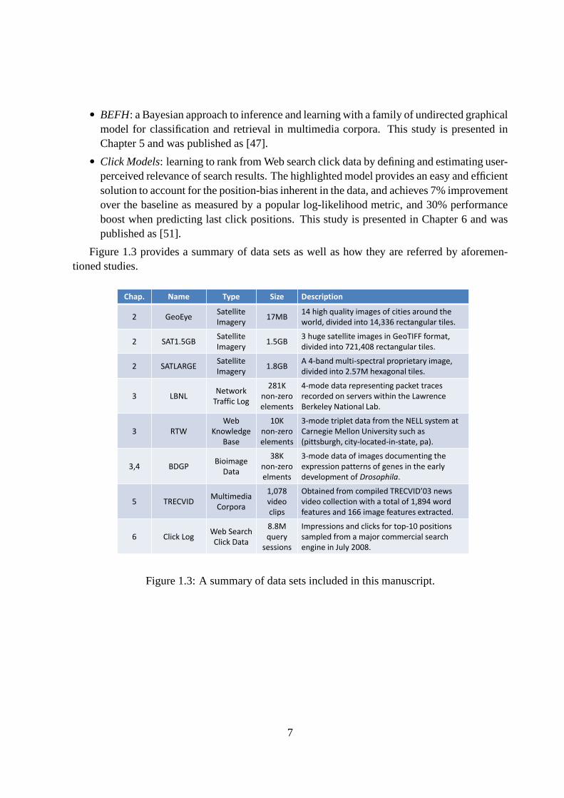
Figure 1.3 provides a summary of data sets as well as how they are referred by aforemen-tioned studies.

Chap. Name Type Size Description

2 GeoEye Satellite

Imagery 17MB

14 high quality images of cities around the

world, divided into 14,336 rectangular tiles.

2 SAT1.5GB Satellite

Imagery 1.5GB

3 huge satellite images in GeoTIFF format,

divided into 721,408 rectangular tiles.

2 SATLARGE Satellite

Imagery 1.8GB

A 4-band multi-spectral proprietary image,

divided into 2.57M hexagonal tiles.

3 LBNL Network

Traffic Log

281K

non-zero

elements

4-mode data representing packet traces

recorded on servers within the Lawrence

Berkeley National Lab.

3 RTW

Web

Knowledge

Base

10K

non-zero

elements

3-mode triplet data from the NELL system at

Carnegie Mellon University such as

(pittsburgh, city-located-in-state, pa).

3,4 BDGP Bioimage

Data

38K

non-zero

elments

3-mode data of images documenting the

expression patterns of genes in the early

development of Drosophila.

5 TRECVID Multimedia

Corpora

1,078

video

clips

Obtained from compiled TRECVID’03 news

video collection with a total of 1,894 word

features and 166 image features extracted.

6 Click Log Web Search

Click Data

8.8M

query

sessions

Impressions and clicks for top-10 positions

sampled from a major commercial search

engine in July 2008.

Figure 1.3: A summary of data sets included in this manuscript.

7

Part II

Mining Multimedia Data

9

Chapter 2

QMAS: Querying, Mining AndSummarization of Multi-modal Databases

Given a large collection of images, very few of which have labels, how can we guess the labelsof the remaining majority, and how can we spot those images that need brand new labels, distinctfrom the existing ones? Current automatic labeling techniques usually scale super linearly withthe data size, and/or they fail when the amount of labeled data is very limited. In this chapter,we introduceQMAS(Querying, Mining And Summarization of multi-modal databases), a fastsolution to the following problems:• low-labor labeling– given a collection of images,very fewof which are labeled with

keywords, find the most suitable labels for the remaining ones;• mining and attention routing– in a similar setting, find clusters and representative images

for each cluster, as well as a set of outlier images.

This chapter is based upon the work published in [30] and [31]. The rest of this chapter is orga-nized as follows: we start with an overview of the proposed approach in Section 2.1, followed bydiscussion of related work in Section 2.2. Algorithmic details are presented in Section 2.3, andempirical results are covered by Section 2.4. Section 2.5 concludes the chapter.

2.1 Overview

The problem of automatically analysis, labeling and understanding large collections of imagesappears in numerous fields. Our driving application is related to satellite imagery, involving ascenario in which a topographer wants to analyze the terrains in a collection of satellite images.We assume that each image is divided into smaller tiles (say,16x16 pixels). Such a user wouldlike to make the effort to create labels (e.g., Water, Concrete, Trees, etc) for only a small numberof tiles, and then expect an automatic algorithm to generatelabels for all the rest. The user wouldalso like to know what pieces of land exist in the analyzed regions look “strange”, not matchingany of the known labels, since they may indicate anomalies (e.g., de-forested areas, potentialenvironmental hazards,etc.), or errors in the data collection process. Finally, the user would like

11

Figure 2.1: An illustration of labeling results from the proposed algorithm. Left: the inputsatellite image of the city of Annapolis, divided in1, 024 (32x32) tiles, only four of which arelabeled. Right: suggested labels fromQMAS; yellow indicates outliers which are likely to repre-sent “Bridge”.

to have a few tiles that best represent each kind of terrain.Such requirements are not only limited to satellite image analysis but also arise in several

other applications including medical image and biologicalimage pattern analysis. For instance,a doctor wants to find tomographies similar to the images of his/her patients as well as a fewexamples that best represent both the most typical and the most strange image patterns [32, 66],or a biological expert with a set of imaging data such as the expression pattern in the earlydevelopment of fruit fly embryos [106] may need a system to answer a similar set of questions.

Our goals are summarized in two research problems:• low-labor labeling– given a collection of images, up to a few of which are labeleda priori,

find the most appropriate labels for remaining ones.• mining and attention routing– in a similar setting, find clusters, a set of images that best

represent the data patterns and another set which consists of top outliers which stand outfrom existing patterns with labels.

Figure 2.1 illustrates the input and output of the proposed algorithm for low-labor labeling.The satellite image, public available atwww.geoeye.com, displays part of the city of An-napolis, MD, USA. We split it into1, 024 (32x32) tiles, very few (four) of which were manuallylabeled as “City” (red), “Water” (cyan), “Urban Trees” (green) or “Forest” (black), as shown onthe left figure. QMASautomatically produced the label and results are shown on the right. Avast majority of tiles are correctly labeled, and a few outlier tiles, highlighted in yellow, are alsopicked up, with the implication that they possibly deserve new label(s) of their own. A closer in-

12

spection in this example concluded that the outlier tiles tend to lie on the border between “Water”and “City”, and are likely to contain a bridge.

For the problem ofmining and attention routing, we take the approach of finding clusters inthe data without the information from the user-provided labels at the beginning. The pure image-based results may be aligned and compared with the evidence from existing labels, possiblyleading to suggestions for refinement such as merging too specific labels that are difficult to bedifferentiated in practice (e.g., “Forest” and “Urban Trees”), and/or splitting too generallabelsof which tiles are not quite alike (e.g., “Shallow Water” and “Deep Sea” could replace a singlelabel of “Water”). Another advantage it offers is that it enables group labeling – the labeling unitcould be a cluster instead of a single tile.

Table 2.1 provides a list of most common acronyms appearing in this chapter.

Table 2.1: Summary of AcronymsAcronym Explanation

ANN Approximate Nearest-Neighbor, an algorithm for fast nearest-neighbor searchingGBT Generalized Balanced Ternary, a hexagonal mathematical system for feature extractionGCap Graph-based automatic image captioning, the baseline image annotation algorithmMrCC Multi-resolution Correlation Cluster detection, a scalable subspace-clustering method[32]RWR Random Walk with Restart for establishing proximity between pairs of nodes in graphViVo Visual Vocabulary, an algorithm to group image tiles into a set of visual terms

2.2 Related Work

2.2.1 Image Labeling

There is an extensive body of work on the classification of unlabeled regions from partiallylabeled images in the field of computer vision, such as image segmentation and region classifica-tion [46, 69, 98, 110]. The conditional random fields (CRF) and boosting approach in [98] showsthe competitive accuracy for multi-class classification and segmentation, but it is relatively slowand requires a lot of training examples to get started. The random walk segmentation methodin [46] is closely related to our work, but scalability is beyond the scope of that work since itis concerned with the segmentation of a single image. The KNNclassifier in [110] may be thefastest way for region labeling, but it may be sensitive for outliers. The empirical Bayes approachin [69] is able to learn contextual information from unlabeled data. However, it may be difficultto apply to satellite image sets.

Graph-based methods provide a flexible tool for automatic image captioning. Images andcaption keywords are represented by multiple layers of nodes in a graph. Image content simi-larities are captured by edges between image nodes, and existing image captions become linksbetween corresponding images and keywords. Such techniques have been previously used inGCap [84], in which a tri-partite graph was built based on captioned images, further segmented

13

into regions. Given an image node of interest, the Random Walk with Restart (RWR) algorithm,which resembles semi-supervised label propagation on graphs [120], was used to perform prox-imity query to automatically find the best annotation keyword for each region. RWR is usuallycomputed using the power iteration method, which convergesin a few iterations in most cases.Another alternative algorithm for labeling is the transductive support vector machine, which hasbeen shown to be efficient and accurate for data which comes with very high dimension andsparse features like word counts [59]. In the satellite imagery we studied in this chapter, thenumber of dimensions does not go beyond a few dozen and certain features may be irrelevant tothe labeling class.

To create edges between similar image nodes, most previous work searches for nearest neigh-bors in the image feature space. However, this operation is super-linear even with the speed upoffered by many approximate nearest-neighbor finding algorithms (e.g., the ANN Library [80]).Given millions of image tiles in satellite image analysis, greater scalability is almost mandatory.

2.2.2 Clustering

Most clustering algorithms assume the following cluster definition: a cluster is a region in thefeature space in which the objects are dense. This region mayhave an arbitrary shape, and thepoints inside it may be arbitrarily distributed.k-means like methods start by pickingk pointsin the metric space as cluster centers, or centroids, through a random process or by applyingsome specific heuristics for this task. The clustering is made possible by an iterative process thatassigns objects to their closest centroids, and iteratively improving the centroids according to theobjects assigned to each cluster. The computation stops when a quality criterion is satisfied orwhen a maximum number of iterations is achieved. An example of this approach is K-HarmonicMeans [117]. The main drawbacks of this approach are that it assumes that the clusters havehyper-spherical shapes in the data space and that the numberk of clusters should be determinedby the usera priori.

The Visual Vocabulary (ViVo) [14] method is particularly useful for our work. ViVo is a novelapproach, proposed for the analysis of biomedical images, that applies Independent ComponentAnalysis (ICA) to group image tiles into a set of visual terms, avoiding subtle problems, such asnon-Gaussianity.

2.2.3 Feature Extraction

Feature extraction is generally considered to be a low-level image processing task and is closelyrelated to feature detection. Histogram-based features are perhaps the simplest and most populartype of features. Texture-based features such as wavelets and fractals are able to capture moresubtle spatial variations such as repetitiveness. Local feature descriptors such as SIFT [74] andSURF [12] have also been widely used, as well as the Generalized Balanced Ternary (GBT) [44],a hexagonal mathematical system that allows feature extraction. A recent example of GBT’susage in target recognition is found in [45]. The choice of candidate features is usually domain-specific and may also be subject to scalability constraints in large scale analysis. The feature

14

"#$

%&'

(')'*#+,+-./!0%#)/12

34.#$5!6-%.'$/5

7#&&/+/5!6#"!

*1#$&8-1%#*'-$

Figure 2.2: Pre-processing applied to multi-band satellite imagery. Best viewed in colors. Left:sample input multi-band image; Right: the resulting 5-bandcomposite image for which featuresare computed.

extraction procedures applied in our study will be introduced in the next section.

2.3 Proposed Method

In this section we discuss algorithmic details ofQMAS, starting with the feature extraction pro-cedure to obtain a compact yet informative representation of image pixels. Then procedures formining and attention routings are introduced, which include clustering, representative identifica-tion and outlier discovery. The low-labor labeling technique is presented in sequel.

2.3.1 Feature extraction

Two approaches feature extraction were employed for different data sets. For public availableimage collections, we obtained Haar wavelets in two resolution levels, plus the mean value ofeach band of the images. For proprietary image collections,we applied an alternative approach:first, there was a pre-processing step resulting in a 5-band composite image as illustrated inFigure 2.2. The first four bands are the 4-band tasseled cap transformation (TCT) of 4-bandmulti-spectral data, and the fifth band is the panchromatic band.

Feature generating following this second approach utilizes a variety of characteristics, in-cluding statistical measures, gradients, moments, and textual measures. For multi-scale imagecharacterization, which is crucial for finding patterns at various resolutions, we adopted General-ized Balanced Ternary (GBT). We mapped the raster pixel datainto the GBT space and calculated

15

! !

Figure 2.3: GBT structure illustrated. Left: two levels of GBT cells with 343 pixels (Level-3,outlined in white) and 2,401 pixels (Level-4, outlined in red) overlaid on an image. Right: outputvalues were assigned according to the variance of the adjacent lower level of cells (at Level-2,consisting of 49 pixels each). Bright areas have greater variance, dark areas have less.

a set of moments-based features over the multi-scale hierarchy of GBT cells. The GBT structureis such that any cell or aggregate at a given layer in the hierarchy contains seven hexagonallygrouped aggregates or hexagons (if at the pixel level) in thelayer below it. The cells form ahexagonal tiling of the pixels at a variety of scales, effectively describing the image in multipleresolutions. A sample of GBT structure and simple computations is shown in Figure 2.3.

Image features such as mean, variance, and GBT texture are calculated for GBT aggregatesin each of the five bands of data. The final feature set comprises a 30-dimensional feature vectorper aggregate: mean, variance, and GBT texture of the Level-n aggregate in each of the five databands plus the mean, variance, and GBT texture of the Level-n + 1 aggregate centered at thatLevel-n position in each of the five data bands.

Following this feature extraction, we adapted the ViVo method [14] to group image tiles intoa set of visual terms, with a slight modification to incorporate GBT aggregate features. If a tilecannot be represented by the vocabulary already known to ViVo, then it will automatically derivea new type of tiles (represented by a new visual term), as needed. These new types representnatural groupings of tiles in the feature space and indicatewhere new labels could potentiallyimprove the accuracy ofQMAS.

2.3.2 Mining and Attention Routing

Clustering

We start by clustering image tiles and subsequently determine representatives and outliers basedon the output. The clustering step over the set of imagesI is performed by a modified version of

16

the MrCC algorithm. As described in Section 2.2, MrCC is a fast subspace clustering algorithmdesigned to look for clusters in large collections of medium-dimensionality data. The originalMrCC algorithm is composed of three main steps: (i) data structure construction; (ii) identifica-tion of initial clusters, namedβ-clusters, which are axis-parallel hyper-rectangles withhigh datadensities; and (iii) overlappingβ-clusters merging. Here we bypass the third step to obtain “soft”clusters, where a single tile can belong to one or more clusters, such as “Trees” and “Water”.

Finding Representatives

Now we focus on the problem of selecting a set of elementsR, of sizeNR specifieda priori,to represent a given set of imagesI. The set of representativesR should have the followingproperty: for every imageIi in I there should be a representativeRr fromR that is mostly similarto Ii. Assuming that these images are already embedded in a metricspace, a straightforwardoptimization goal is to minimize the sum of squared distances between each imageIi and itsclosest representativeRr. The solution is simply the popular clustering algorithm K-means.However, the method is known to be sensitive to skewed distributions, data imbalance,etc, whichis not uncommon for our use case in studying the satellite imagery. Here we propose to optimizethe following dis-similarity function instead:

EQMAS(I, R) =∑

Ii∈I

NR∑NR

j=11

‖Ii−Rj‖2

(2.1)

Therefore, instead of focusing on the minimum of distance between the target image and repre-sentatives, here the harmonic mean is the concern, which is usually more robust to extreme datadistributions and unfortunate initializations. The solution to this metric is known as K-harmonicmeans [117].

Finding Outliers

The goal in this part is to find an ordered list of potential outliers, images ofI that diverge mostfrom main data patterns. We take the representatives found in the previous section as the basisfor the outliers definition,i.e., assuming that a set of representativesR is a good summary ofI, theNO images fromI worst represented byR are said to be the top-NO outliers. Formally,QMASuses the harmonic mean of the squared distances between an imageIi and each one of therepresentatives inR to measure the quality of the representation ofIi, therefore the top outlier isidentified by

argmaxi

NR∑NR

j=11

‖Ii−Rj‖2

(2.2)

2.3.3 Low-labor Labeling

Our approach is to represent input images and labels, together with the image clusters foundbefore, in a graphG, known as theknowledge graph. A random walk-based algorithm is applied

17

overG to find the most appropriate labels for the unlabeled images.Algorithm 1 shows a sketchof our solution, and details are given in the remainder of this subsection.

Algorithm 1 : QMAS labeling.Input: collection of imagesI;

collection of known labelsL;restart probabilityc;clustering outputC.

Output: full set of labelsLF .1: useI, L andC to build the graphical representationG;2: for each unlabeled imageIi ∈ I do3: random walk over graphG from vertexV (Ii), and with

probabilityc, restart the walk fromV (Ii) again;4: compute the affinity between each label ofL andIi using power iteration method imple-

menting a revised random walk with restart algorithm;5: let Ll be the one with the largest affinity value in set inL, thenLFi ← Ll;6: end for7: return LF ;

G is a tri-partite graph that consists of the vertex setV and the edge setE. V is made upof three layers corresponding to the input imagesI, the clusters of imagesC, obtained withalgorithms described in Section 2.3.2, and the set of image labelsL. Vertices inG that representimageIi and labelLl are denoted byV (Ii) andV (Ll), respectively. It is self-evident that withclustering results in hand, the construction process of such a graphG is linear in time and space.Figure 2.4 exemplifies a toy graph with seven images, two distinct labels, and three clusters.ImageI1 is pre-labeled withL1, while I4 andI7 are both pre-labeled withL2. Note that underthe soft clustering scheme we adopted, an image node may be linked with more than one nodesrepresenting clusters,e.g., I3 is connected to bothC1 andC2.

Given an unlabeled imageIi, we apply the following algorithm over the graphG in orderto find an affinity score for each possible label with respect to Ii; it is imitating the well-knownrandom walk with restart algorithm with a minor modificationon selecting the random neighborto land on. The random walker starts from vertexV (Ii) initially. At each time step, the walkeralways takes one of the following two choices: (1) go back toV (Ii), with probabilityc; (2) walksto a neighboring vertex, with probability1− c. Under the latter case, the probability of choosinga neighboring vertex is proportional to the degree of that vertex, i.e., the walker favors smallerclusters and more specific labels. The value ofc is usually set to an empirical value (e.g., 0.15), ordetermined by cross-validation. The affinity score forLl with respect toIi is given by the steadystate probability that our random walker will find himself atvertexV (Ll), always restarting atV (Ii). The label with the largest score becomes the recommended label for Ii.

The intuition behind this procedure is that similar images that belong to the same clustershould share similar labels. This is consistent with our graph proximity measure which favorsmultiple short paths between the two vertices of interest. For instance, consider imageI6 in

18

!

"#! "$! "%!

&#! &$! &%! &'! &(! &)! &*!

+#! +$!

Figure 2.4: The knowledge graph for a toy input set. Nodes shaped as squares, circles, andtriangles represent images, labels, and clusters respectively.

Figure 2.4. It belongs to clustersC2 andC3. The other two images inC3 bear labelL2, whereasnone of the images inC2 is labeled. Hence there is a higher probability that a randomwalkerstarting fromV (I6) will reachV (L2) thanV (L1), in that there are two shortest paths of length3 linking V (I6) andV (L2), whereas the only shortest path connectingV (I6) to V (L1) takes asmany as 5 steps. Moreover, the affinity score forL2 could be higher ifI6 were associated withC3 only. Thus, for larger graphs, in which it is not untypical that an image belongs to multipleclusters, the membership with a smaller cluster takes more weight than that with a larger one.

2.4 Experimental Results

2.4.1 Experimental Setup

We first introduce three data sets of satellite images that serve at the test beds in this section:• GeoEye– 14 high quality satellite images in JPEG format of a number of cities around the

world. The total size of these images is17 MB. We divided each image into equal-sizedrectangular tiles and yielded a total of14, 336 tiles. Figure 2.1 includes a snapshot of1, 024

tiles.• SAT1.5GB– the data set is made up of three satellite images in the GeoTIFF format, each

of size∼ 500MB. The total number of equal-sized rectangular tiles is721, 408.• SATLARGE– this proprietary data set contains a pan QuickBird image ofsize 1.8 GB,

and its matching 4-band multi-spectral image of size 450 MB each. These images were

19

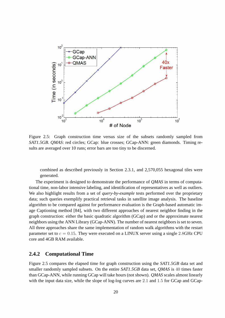
Figure 2.5: Graph construction time versus size of the subsets randomly sampled fromSAT1.5GB. QMAS: red circles; GCap: blue crosses; GCap-ANN: green diamonds. Timing re-sults are averaged over 10 runs; error bars are too tiny to be discerned.

combined as described previously in Section 2.3.1, and 2,570,055 hexagonal tiles weregenerated.

The experiment is designed to demonstrate the performance of QMASin terms of computa-tional time, non-labor intensive labeling, and identification of representatives as well as outliers.We also highlight results from a set ofquery-by-exampletests performed over the proprietarydata; such queries exemplify practical retrieval tasks in satellite image analysis. The baselinealgorithm to be compared against for performance evaluation is the Graph-based automatic im-age Captioning method [84], with two different approaches of nearest neighbor finding in thegraph construction: either the basic quadratic algorithm (GCap) and or the approximate nearestneighbors using the ANN Library (GCap-ANN). The number of nearest neighbors is set to seven.All three approaches share the same implementation of random walk algorithms with the restartparameter set toc = 0.15. They were executed on a LINUX server using a single2.8GHz CPUcore and 4GB RAM available.

2.4.2 Computational Time

Figure 2.5 compares the elapsed time for graph constructionusing theSAT1.5GBdata set andsmaller randomly sampled subsets. On the entireSAT1.5GBdata set,QMASis 40 times fasterthan GCap-ANN, while running GCap will take hours (not shown). QMASscales almost linearlywith the input data size, while the slope of log-log curves are 2.1 and1.5 for GCap and GCap-

20

Figure 2.6: Labeling accuracy versus the number of pre-labeled examples for each labeling class.QMAS: red circles; GCap-ANN: green diamonds. Accuracy values ofQMASare barely affectedby the size of the pre-labeled data. Box plots summarize 10 runs over randomly selected inputs,with outliers (typically over 3 standard deviations from the mean) indicated by red circles andgreen diamonds.

ANN, respectively. Instead of performing nearest neighborsearches, which is super-linear evenwith a state-of-the-art approximation algorithm,QMASemploys a linear-time clustering algo-rithms to leverage the content similarity in satellite image tiles, and achieves superior scalability.

2.4.3 Non-labor Intensive Labeling

We manually labeled 256 tiles in theSAT1.5GBdata set as the ground truth. By randomly choos-ing a small number of these labels as input and leaving out remaining ones for evaluation, wecompare the labeling accuracy of the three approaches from 10 repetitive runs and display qual-ity results as box plots in Figure 2.6.QMASdoes not sacrifice quality for faster computationaltime when compared with GCap-ANN, and it actually performs even better when the size of thepre-labeled data is limited. Additional experiments have shown given10 pre-labeled examplesfor each class, even under the optimal performance-speed trade-off for GCap-ANN, where thenumber of nearest neighbors set to three,QMASis still 1.75 times faster and around10% moreaccurate. Note that the accuracy ofQMASis barely affected by the number of the pre-labeledexamples in each label class. The fact that it can still extrapolate from tiny sets of pre-labeleddata ensures its non-labor intensive capability.

21

Figure 2.7: Representatives for theGeoEyedataset, each colored according to the cluster mem-bership.

Figure 2.8: Top-3 outliers for theGeoEyedataset.

2.4.4 Finding Representatives and Outliers

Figure 2.7 shows data representatives obtained on theGeoEyedata set. A total of6 representa-tives are displayed, which are colored according to their clusters. Note that a large cluster, suchas “Water”, may have multiple representatives.

Figure 2.8 presents the top-3 outliers on the same data set. Closer inspection found that theseoutlier tiles tend to be on the border of areas like “water” and “city”, where a bridge usuallyappears. These3 outlier tiles, together with6 representatives, compactly summarize theGeoEyedata set, which contains more than14 thousand tiles.

22

Figure 2.9: Example “Water”: Labeled Data and Results of Water Query.

Figure 2.10: Example “Boats”: Labeled Data and Results of Boat Query.

23

2.4.5 Query-by-Example Experiments

The query-by-example experiments were carried out for the proprietarySATLARGEdata set bydomain experts in satellite image analysis. Given a small set of tiles asexamples, they would liketo find most similar tiles over the entire data set. To applyQMAS, the given tiles are assigned witha single label, and we performed random walk based algorithms to find tiles, other than thosealready given, that are mostly similar to this label. For instance, Figures 2.9 and 2.10 exemplifythe results obtained for “Water” and “Boats”, respectively. We also varied the size of the pre-labeled data in these experiments between one and fifty, to observe how the system respondedto these changes. In general, labeling only small numbers ofexamples(even less than five)stillleads to accurate results; when the number was reduced to2, we began to see the negative effectsof having an exceedingly small input set.

Notice that correct returned results often look very different from the given samples,i.e.,the system is able to extrapolate from the given examples to other, correct tiles that do not havesignificant resemblance to the pre-labeled set. Clearly, this is not a typical automated targetrecognition (ATR) approach. There are no “templates” and nospecific object shapes, orienta-tions, sizes, or patterns that are learned. Unlike a traditional ATR that typically fails when itencounters an object that does not fit the specified description, QMASis able to correctly labelan object that has a somewhat different appearance from the “known” set.

2.5 Conclusion

In this chapter we proposedQMAS, a fast solution to low-labor labeling, mining and attentionrouting for multi-modal databases. We carried out experiments in the scenario of satellite imageanalysis to evaluate its performance.QMASscales linearly over the size of the data set, beingmultiple times faster than an alternative algorithm in graph construction. At the same time, itprovides high quality labeling results, even with tiny setsof pre-labeled data as inputs. It couldalso spot top representatives and outliers and offered a compact summarization of a large data set.The implementation was also employed to perform a set of practical queries over a proprietarydata set by domain experts and it yielded quite positive results – QMASis able to correctly labelan object where the traditional automated target recognition (ATR) approach may fail.

Future directions include leveraging the locality within images,i.e., the fact that image tilesthat are neighbors are more likely to share similar labels, and generalizing the method to handlean ontology of labels.

24

Chapter 3

MultiAspectForensics: Pattern Mining onLarge-scale Heterogeneous Networks withTensor Analysis

Modern applications such as web knowledge base, network traffic monitoring and online socialnetworks have made available an unprecedented amount of network data with rich types of in-teractions carrying multiple attributes, for instance, port number and timestamp in the case ofnetwork traffic. The design of algorithms to leverage this structured relationship with the powerof computing to assist researchers and practitioners for better understanding, exploration andnavigation of this space of information has become a challenging, albeit rewarding, topic in so-cial network analysis and data mining. The constantly growing scale and enriching genres ofnetwork data always demand higher levels of efficiency, robustness and generalizability whereexisting approaches with successes on small, homogeneous network data are likely to fall short.

MultiAspectForensics, introduced in this chapter, is a handy tool to automatically detect andvisualize novel subgraph patterns within a local communityof nodes in a heterogeneous network,such as a set of vertices that form a dense bipartite graph whose edges share exactly the same setof attributes. We apply the proposed method on three data sets from distinct application domains,present empirical results and discuss insights derived from these patterns discovered. Our algo-rithm, built on scalable tensor analysis procedures, captures spectral properties of network dataand reveals informative signals for subsequent domain-specific study and investigation, such assuspicious port-scanning activities in the scenario of cyber-security monitoring.

This chapter will be structured as follows: we first motivatethe discussion in Section 3.1, andthen elaborate onMultiAspectForensicsprocedures step-by-step in Section 3.2. Empirical resultsare presented in Section 3.3. And related literatures are briefly sketched in Section 3.4. Lastly,Section 3.5 concludes the chapter and highlights future directions. Most of the work describedsubsequently is based on the material presented in [75].

25

3.1 Introduction

Modern applications in the Internet era, either data-informed or data-driven, have contributed tothe boom of network data arising from a spectrum of domains, such as web knowledge base,network traffic monitoring and online social networks. A glowing trend in the accumulationand analysis of such data is the emergence of heterogeneous interactions between nodes in thenetwork, for which a vivid depiction is offered by the Facebook friendship page, with multiplepage elements ranging from wall posts, comments, and photos, to mutual friends, shared inter-ests and common networks between a pair of users. Browsing and navigation over such a spaceof information, despite its overwhelming scale and complexity, has been a challenging task com-mon encountered in many fields. Yet the rather recent availability and popularity of these data,in addition to practical requirements over the efficiency, robustness and generalizability of thesolution, has rendered the topic of pattern mining for heterogeneous network data a relativelyunderexplored one, where even the definition of interestingor abnormalpatternscould becomea non-trivial problem itself.

Many of pioneering studies on pattern discovery for graph and network data focused onfrequent substructure mining, with heuristics motivated by information theory [29], mathematicalgraph theory [67, 116], inductive logic programming [35], etc. An intimately related problemis the detection of rare event and anomalous behavior, whichhas attracted wide interests thanksto its many well-recognized applications concerned with security, risk assessment, and fraudanalysis. Noble and Cook [82] were among the first to address this challenge on structurednetwork data by providing solutions based on the minimal description length principle to searchfor abnormal subgraphs. And many alternative approaches are now available to spot anomalousnodes [6], edges [24], or both [38], with further elaboration adapted to bipartite graphs [103],and time-evolving graphs [109]. This piece of work, by revealing two classes of patterns inthe context of heterogeneous graphs, resembles a novel attempt to explore this relatively youngrealm of multi-aspect network data for state-of-the-art discoveries and developments.

We resort to a tensor-based representation for heterogeneous network data and employ off-the-shelf decomposition algorithms [64] as a starting point of the analysis. Previous researchalong this line has paid a great deal of attention on individual nodes, which play a central role insimilarity ranking [41], personalized recommendation [118], etc. The major finding in our studyis that, for multiple heterogeneous network data across diverse application domains, we couldalways observe groups of elements with similar connectionsalong one or more data modes,as implied by nearly-identical decomposition scores, which transform to quite visible spikes inhistogram plots. While algorithms in aforementioned studies mostly look for elements with topeigenscores, our heuristic distinguishes itself bybeing able to capture patterns formed by lesswell-connected nodes in the network, which do not necessarily stand out in the eigenspace andare often ignored by other extant techniques.

In summary,MultiAspectForensicsstarts with a data decomposition step for input heteroge-neous networks, features a spike detection heuristic to reveal non-trivial substructure patterns,and also includes programs to automatically visualize the findings. We demonstrate its effec-tiveness and efficiency by executingMultiAspectForensicson three data sets from distinct appli-

26

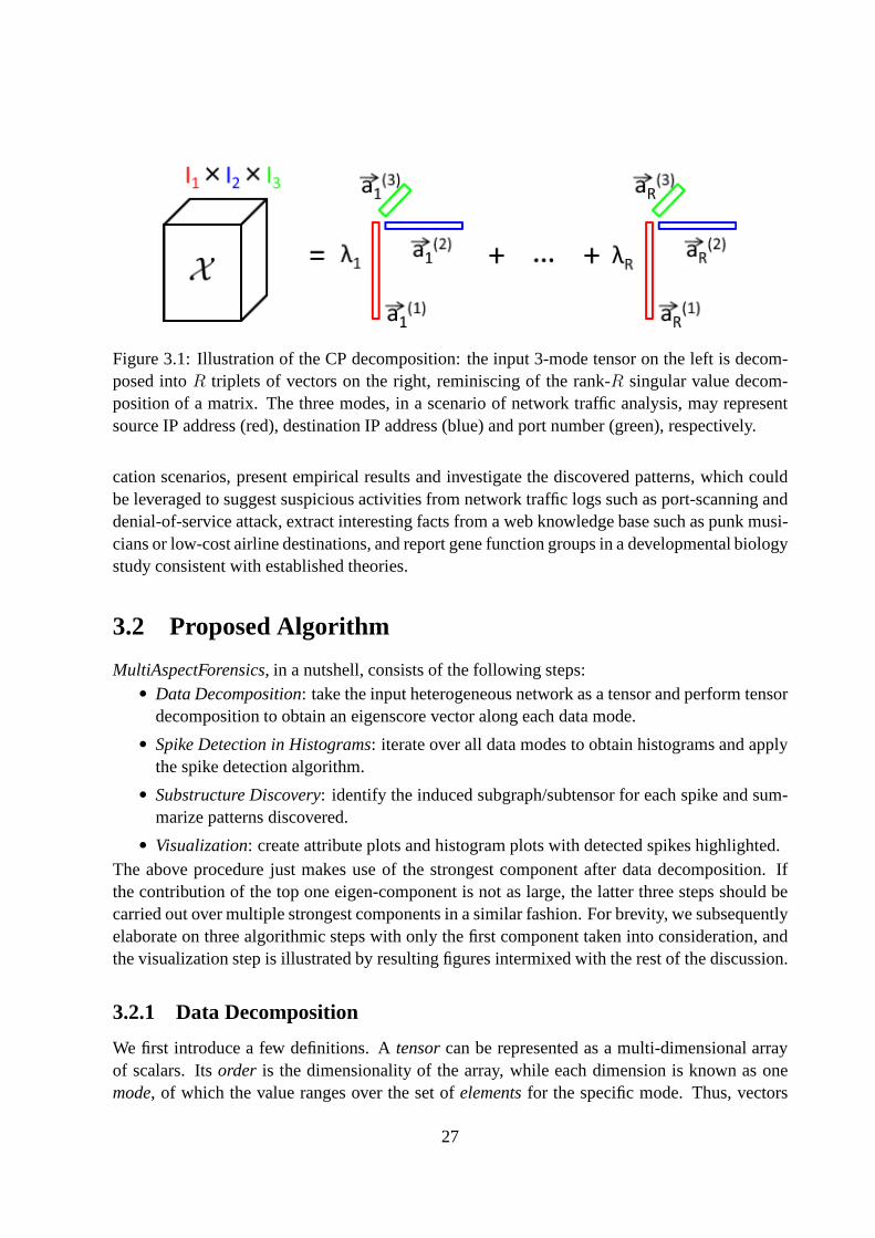
Figure 3.1: Illustration of the CP decomposition: the input3-mode tensor on the left is decom-posed intoR triplets of vectors on the right, reminiscing of the rank-R singular value decom-position of a matrix. The three modes, in a scenario of network traffic analysis, may representsource IP address (red), destination IP address (blue) and port number (green), respectively.

cation scenarios, present empirical results and investigate the discovered patterns, which couldbe leveraged to suggest suspicious activities from networktraffic logs such as port-scanning anddenial-of-service attack, extract interesting facts froma web knowledge base such as punk musi-cians or low-cost airline destinations, and report gene function groups in a developmental biologystudy consistent with established theories.

3.2 Proposed Algorithm

MultiAspectForensics, in a nutshell, consists of the following steps:• Data Decomposition: take the input heterogeneous network as a tensor and perform tensor

decomposition to obtain an eigenscore vector along each data mode.

• Spike Detection in Histograms: iterate over all data modes to obtain histograms and applythe spike detection algorithm.

• Substructure Discovery: identify the induced subgraph/subtensor for each spike and sum-marize patterns discovered.

• Visualization: create attribute plots and histogram plots with detected spikes highlighted.The above procedure just makes use of the strongest component after data decomposition. Ifthe contribution of the top one eigen-component is not as large, the latter three steps should becarried out over multiple strongest components in a similarfashion. For brevity, we subsequentlyelaborate on three algorithmic steps with only the first component taken into consideration, andthe visualization step is illustrated by resulting figures intermixed with the rest of the discussion.

3.2.1 Data Decomposition

We first introduce a few definitions. Atensorcan be represented as a multi-dimensional arrayof scalars. Itsorder is the dimensionality of the array, while each dimension is known as onemode, of which the value ranges over the set ofelementsfor the specific mode. Thus, vectors

27

are tensors of order one, and matrices are tensors with two modes. In Section 3.3 we will usemeasureto denote the unit of eachentry in the multi-dimensional array.

To transform a heterogeneous network into a tensor, every edge becomes a non-zero entryin the multi-dimensional array, where edge attributes, together with edge source and destination,make up different modes of the tensor. Edge weights naturally stay as entry values for weightednetworks. Node attributes could also be incorporated by taking a Cartesian product over two endpoints of an edge, for instance, if a directed network contains nodes with7 different colors, wecould have an edge attribute whose arity is72 = 49.

Tensor decomposition leverages multi-linear algebra to the analysis of high-order data. Thecanonical polyadic (CP) decomposition we applied in this chapter generalizes the singular valuedecomposition (SVD) for matrices. It factorizes a tensor tothe weighted sum of outer products ofmode-specific vectors, as illustrated in Figure 3.1 for a 3-order tensor. Formally, for anM-modetensorX of sizeI1 × I2 × · · · × IM , its CP decomposition of rankR yields

X (i1, . . . , iM) ≈R∑

r=1

λr

(−→a(1)r × . . .×

−−→a(M)r

)

=

R∑

r=1

λr

M∏

m=1

a(m)rim (3.1)

Similar to SVD, the approximation becomes closer asR enlarges, and would be exact if it equalsthe rank of the tensor (see [53] for details).

3.2.2 Spike Detection in Histograms

Now that we have transformed complex structured data into a set of more manageable vectors,the next step is to spot common patterns from these vectors. As a starting point, we visualizeeach vector by creating an attribute plot, which displays absolute values of eigenscores (y-axis)along its elements (indexed by the x-axis). An example of such plots is given in Figure 3.2.Note that the y-axis should be inlog scale to emphasize the relative difference. The arrow onthe right indicates a score value shared by many elements,i.e., a number of entries in the eigen-vector have exact the same values, which is not uncharacteristic in other dimensions and acrossdifferent data sets.This key observationenables us to create effective heuristics to extract spikesfrom histograms and subsequently examine subgraph patterns they imply in the next subsection.And the fact that many spikes do not appear at the very top of the figure with most significanteigenscore values makes it more difficult for many alternative methods to be effective.

Prior to applying the spike detection heuristics, we obtainhistogram data by equally dividingthe range of eigenscores in log scale. The detection algorithm just needs to sort and traverse thehistogram data until one of the following conditions is satisfied: (1) the energy as measured bysum of square values covered is equal or more than a fraction of s, and the magnitude of thespike is less than a fraction ofr than the largest one; (2) there are alreadyK spikes. Parametervalues are empirically set tos = 90%, r = 50%, K = 20, where small variations lead to littleperturbation of the output. The pseudo-code of the algorithm is listed in Algorithm 2 above.

28

Figure 3.2: An attribute plot which displays absolute values of eigenscores (y-axis in log-scale)along its elements (indexed by the x-axis). The arrow on the right points to a common scorevalue, illustrating an observation critical to the algorithmic design ofMultiAspectForensics.

Application of this algorithm to the data vector in Figure 3.2 yields Figure 3.3, where we putattribute plot on the left side-by-side with histogram ploton the right, highlighting every spike inred.

3.2.3 Substructure Discovery

Having extracted sets of elements that form histogram spikes from each data mode, we headback to the input network data to examine corresponding local subnetworks to complete the finalstep of pattern discovery. The running example in this subsection comes from a snapshot ofnetwork traffic log which consists of packet traces in an enterprise network [70]. Each trace inthe log is a triplet of (source-IP, destination-IP, port-number), which could be represented as adirected network of machine IP addresses with the only edge attribute “port number” and numberof packets as edge weights. Patterns derived fromMultiAspectForensicscould be summarizedinto the following two categories:

generalized star

A subnetwork which consists of conterminous edges that differ only in one data mode. For in-stance, a group of source IP addresses sending packets to a single destination server using the

29

Figure 3.3: An attribute plot (adopted from Figure 3.2) on the left side-by-side with the corre-sponding histogram plot with spikes detected indicated by circles.

same port. It generalizes the star pattern in two dimensional graphs, and makes up a continuousblock along one dimension in the adjacency tensor, if elements along that dimension are orderedcarefully. Note that in a heterogeneous network, this category of patterns also includes multipleedges between one pair of nodes with differing attribute values,e.g., a good many port numbersin our running example, in which case the source machine may be either an administrator per-forming port screening or a suspect trying to exploit a vulnerable port. Figure 3.4 provides anillustration of these patterns.

generalized bipartite-core

A subnetwork that represents a dense bipartite structure similar to the bipartite-core pattern inregular graphs, and is akin to association rules as well. More generally, it can be viewed as a con-tinuous block along two dimensions in higher-order tensorsunder specific element orders. Forinstance, a group of source IP addresses sending packets to multiple destination servers with thesame port. Note that in a heterogeneous network, this category of patterns also includes, writtenin the language of network forensics, multiple source IP addresses sending packets over differentport numbers to the same server. This is likely to happen during a DDoS (Distributed Denial-of-Service) attack, a typical scenario of network intrusion, in which source IPs play the role ofmalicious hosts sending huge volumes of packets to the target server as the victim. Figure 3.5provides an illustration of these patterns.

As a final remark, the statement that both patterns are related to a block along one or twodimensions in the high-order tensor only holds when elements of their respective data modes areordered in specific ways. And the complexity to search for such an order is generally exponential,which reflects, in some sense, the power of the proposed approach.

30

Figure 3.4: Examples of generalized star patterns discovered in the LBNL (Lawrence BerkeleyNational Lab) network traffic data set. Wavy arrows indicatemultiple edges between the pair ofnodes with a handful of distinct attribute values. (a) 10 source IP addresses (randomly selectedout of 172 ones) are sending multiple packets to a server machine with Port# 534, which is aUDP port under the NCP protocol from a network OS for file sharing and printing services; (b)The source IP registered by an Indian ISP is sending packets to a host in LBNL via port numbers(ranging from 2,300 to 2,900) not usually intended for this type of communication, implying asuspicious activity.

31

Figure 3.5: Examples of generalized bipartite-core patterns discovered in the LBNL (LawrenceBerkeley National Lab) network traffic data set. Wavy arrowsindicate multiple edges betweenthe pair of nodes with a handful of distinct attribute values. (a) 10 source IP addresses (ran-domly selected out of 119 ones) are sending multiple packetsto an array of server machines,including server 131.243.141.187, which also appears in Figure 3.4 as part of a generalized starpattern, over a port used for file sharing and printing services; (b) 10 source IP addresses (ran-domly selected out of 63 ones) are sending packets over different ports to a multi-purpose servermachine.

32

Algorithm 2 SDA(Spike Detection Algorithm)Input: Eigenscore histogram vectorH of sizeNOutput: The set indicating spikes detectedS

1: S = φ

2: sort the histogram to obtain an ordered vectorHo s.t.Ho1 ≥ Ho2 ≥ · · · ≥ HoN

3: QSUM ←∑N

n=1H2n

4: Q← 0

5: for k = 1, . . . , K do6: S ← S ∪ {ok}7: Q← Q+H2

ok

8: if Q/QSUM ≥ s andH(ok)/H(o1) < r then9: break

10: end if11: end for12: return S

Data set # modes Dimensions Measure# non-zeroelements

LBNL 42,345 source IPs, 2,355dest IPs, 6,055 port #’s,3,610 timestamps

# packets 281K

RTW 33,641 subjects, 3,929 ob-jects, 98 verbs

binary 10K

BDGP 34,491 genes, 248 terms, 6stages

binary 38K

Table 3.1: A Summary of Data Sets

3.3 Empirical Results

We commence this section with the description of data sets aswell as experimental environment.It is followed by the discussion of respective patterns discovered byMultiAspectForensicsin eachof the three data sets.

3.3.1 Data and Environment

Data sets are acquired from three dissimilar application domains: network traffic monitoring,knowledge networks, and bioinformatics. A summary is highlighted in Table 3.1.

LBNL The network traffic log is made available through a research effort to study the char-acteristics of traffic for Internet enterprises [86]. The measurement was taken on serverswithin the Lawrence Berkeley National Lab (LBNL) from thousands of internal hosts overtime, with millions of packet traces recorded. Each packet trace includes four data modes:

33

source IP, destination IP, port number, and a timestamp in second. For privacy reasons,lower 16 bits were randomly permuted to anonymize the host identity, whereas upper 16bits were kept intact for proper identification of the location and service provider [87]. Weborrowed a subset of this data set within 1-hour time span in this section.

RTW This online knowledge base is the outcome of the NELL (Never-Ending Language Learn-ing) system at Carnegie Mellon University [20]. It employs natural language processingand machine learning techniques to constantly and automatically crawl web pages andextract facts [21]. Each fact is a triplet of (subject, verb,object) such as (pittsburgh, city-located-in-state, pennsylvania), which could be represented as a directed graph made up ofentities likepittsburghor pennsylvania, edges with attributes likecity-located-in-state. Forbetter quality of results, we applied our algorithm on a preprocessed subset after manualnoise removal (by courtesy of Bryan Kisiel at Carnegie Mellon University).

BDGP The data set is collected from the Berkeley Drosophila Genome Project (BDGP) to studythe spatial-temporal patterns of gene expression during the early development of fruitfly [106, 107]. We selected three data modes from the databasedump available at [13],which consists of 4,491 genes, 248 functional annotation terms from a specialized vocab-ulary, and 6 different developmental stages.

MultiAspectForensicswas implemented in the MATLAB language, and all following exper-iments were performed on a Unix machine with four 2.8GHz cores, and 16GB memories. Forevery of these data sets, the wall-clock time was no more than2 minutes to carry out the compu-tation and generate attribute plots and histogram plots along all modes.

3.3.2 LBNL Traffic Log

We have already discussed patterns discovered from a snapshot of this data set in Section 3.2.3,illustrated in Figures 3.4, 3.5. With the additional mode oftimestamp, we found two dominatingspikes in its histogram plot. Upon closer examination, we reported the following activities: thefirst spike is a generalized bipartite-core pattern relatedto the HTTP traffic on port 80 betweenfour servers in LBNL and three remote hosts in Chinese academic institutions, possibly executingscripts to crawl/download web pages. The second spike represents a generalized star patternbetween one of the local HTTP server and the same remote host at India aforementioned. Wetraced further in time and found that the remote host never sent packets back to acknowledge theconnection, suggestive of suspicious activities to be reported to domain experts.

3.3.3 RTW Knowledge Base

Recall that each item in the knowledge database could be represented as a (subject, verb, object)triplet. MultiAspectForensicsdetected spikes mostly on data modes representing subjectsandobjects.

Figure 3.6(a) illustrates a subgraph discovered revealinga generalized star pattern. The mu-sic artists/bands listed here are specialized to punk musicor its sub-genres (not shown in the

34

(a) Punk Music (b) European Cities

Figure 3.6: Two generalized star patterns discovered from the RTW knowledge base: (a) Musicartists specialized in punk or one of its sub-genres according to the knowledge base; (b) Europeandestinations of the Ryanair, an Irish low-cost airline.

figure) according to the knowledge base, whereas their more versatile peers will not be favorablyselected byMultiAspectForensics.

Figure 3.6(b) displays another generalized star pattern between European cities and an Irishlow-cost airline which flies to many regional or secondary airports to reduce cost, following adifferent business model and choice of destination from industrial giants.

The evidence here and many others alike could also be leveraged in a variety of graph miningtasks on this knowledge base such as clustering entities or creating an ontology between them,given the fact that nodes within the same spike tend to behavesimilarly and specifically. More-over, as a sanity check, since node names are ordered alphabetically in this data set, the patterndoes not make a continuous block in the tensor without non-trivial permutation.

3.3.4 BDGP Gene Annotation

In this data setMultiAspectForensicsspots a set of genes known to be responsible for themater-nal effectin the early development of fruit fly (Figure 3.7), which alsoprovides hints to studyother higher organisms includingHomo sapiens. Products of such maternal effect genes, in theform of either protein or mRNA, play a critical role in the very early stage of embryo devel-opment, such as the first few cell divisions. For instance, four of such genes, includingbicoid,caudal, hunchback, andnanos, is mostly responsible for the determination of anterior-posterioraxis – which side of the embryo will be the future head and which other side will be the futuretail [68].

35

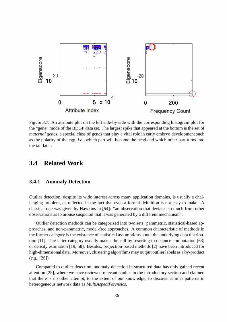
Figure 3.7: An attribute plot on the left side-by-side with the corresponding histogram plot forthe “gene” mode of the BDGP data set. The largest spike that appeared at the bottom is the set ofmaternal genes, a special class of genes that play a vital role in early embryo development suchas the polarity of the egg,i.e., which part will become the head and which other part turns intothe tail later.

3.4 Related Work

3.4.1 Anomaly Detection

Outlier detection, despite its wide interest across many application domains, is usually a chal-lenging problem, as reflected in the fact that even a formal definition is not easy to make. Aclassical one was given by Hawkins in [54]: “an observation that deviates so much from otherobservations as to arouse suspicion that it was generated bya different mechanism”.

Outlier detection methods can be categorized into two sets:parametric, statistical-based ap-proaches, and non-parametric, model-free approaches. A common characteristic of methods inthe former category is the existence of statistical assumptions about the underlying data distribu-tion [11]. The latter category usually makes the call by resorting to distance computation [63]or density estimation [19, 58]. Besides, projection-basedmethods [2] have been introduced forhigh-dimensional data. Moreover, clustering algorithms may output outlier labels as a by-product(e.g., [26]).

Compared to outlier detection, anomaly detection in structured data has only gained recentattention [25], where we have reviewed relevant studies in the introductory section and claimedthat there is no other attempt, to the extent of our knowledge, to discover similar patterns inheterogeneous network data asMultiAspectForensics.

36

3.4.2 Tensor Analysis and Graph Mining

Tensor decomposition has been a basic technique well studied and applied to a wide range of dis-ciplines and scenarios. An informative survey on tensor decompositions is presented by Koldaand Bader [64] with many further references. Recent researches have further generalized theCP decomposition to handle incomplete data [1], or to produce non-negative components [97].Tucker decomposition, as the other well-known approach, ismore flexible, although its applica-tion is usually limited by its limited scalability and vulnerability to noise. Notably, recent workon scalable alternatives such as [111] may open up the venue to enhance theMultiAspectForen-sicsmethodology with more powerful decomposition algorithms.

Quite a few popular implementations of tensor decomposition algorithms for academic re-searchers have been made publicly available. Examples are the N-way toolbox by Anderssonand Bro [7] and the more recent MATLAB Tensor Toolbox by Baderand Kolda [9].

Tensor analysis has also been applied to study the dynamics of graphs and networks [104].They commonly start by analyzing graph/tensor snapshots within each timestamp, and take theoutput for subsequent time-series analysis.MultiAspectForensics, instead of focusing on theevolution between adjacent timestamps, treats timestamp as another data mode to allow betterdiscovery of global patterns in this trade-off.

3.5 Conclusion

We presentedMultiAspectForensics, a handy and effective tool to automatically detect and visu-alize a category of novel patterns, including generalized star and generalized bipartite-core pat-terns, within a local community of nodes in heterogeneous networks, even if they exist amongless-well connected nodes which are more likely to be ignored by many extant methods. Empir-ical results exhibited valuable insights derived from pattern discovered, across multiple applica-tion domains such as network traffic monitoring, knowledge networks, and bioinformatics. Thesesuccesses could be attributed to the fact that we resorted toa tensor-based representation to facil-itate data decomposition, reached a key observation leading to spike patterns in histogram plots,and revealed typical substructures reflecting spectral properties of heterogeneous data. HenceMultiAspectForensicsrealizes an early attempt to research substructure patterns commonly ex-isting in heterogeneous network data, and a reasonable use case of tensor analysis, despite thesimplicity of heuristics resided.

An important problem beyond the scope of this manuscript is the design of an objective andquantitative evaluation framework of discovered patterns, especially for large-scale networks forwhich it is prohibitive to label every interesting pattern.Although it may be relatively to defineprecision and recall by exhaustively searching for subgraphs bearing the specified pattern such asgeneralized star or generalized bipartite core, the definition of quality, or value of these patternsfrom automated discovery, is usually domain and context specific – even may not be losslesslyquantified. This would also shed lights on a principle way of optimizing parameters, yet we foundthat results were usually not sensitive to parameter valueswhen they vary within reasonable

37

ranges. Meanwhile, it’s our plan to open-source theMultiAspectForensicstool based on thegenericboost graph library[99] to make it more accessible and usable by industrial practitionersand academic researchers, and collect feedbacks for possible future developments.

38

Part III

Querying Multimedia Data

39

Chapter 4

CDEM: Flexible Querying System forBiological Image Databases

Given a large collection of images documenting the spatial patterns of gene activities on football-shaped embryos, can we perform content-based retrieval to find similar patterns for an existingor new input? Can we leverage this similarity to group together genes that display correlatedpatterns, which suggests a greater likelihood for them to participate in the same biological pro-cess in the development of the embryo? Can we construct a network of genes to visualize suchrelationships known as co-expression? Moreover, most of the genes bear a handful of labels,manually curated by domain experts using anatomical terms to indicate the body-part (e.g., “em-bryonic hindgut”) with most significant expression activity, can we employ this additional se-mantic information to improve the retrieval results, or automatically assign such labels to newand upcoming images?

This chapter and the accompanying online query interface isan initial attempt to addressthese questions. Part of the work described subsequently isbased on the material presented in[48].

4.1 Background

How an organism develops from a single cell, one of the great mysteries of life, has alwaysbeen an intriguing problem for biologists. To uncover the genetic foundation of animal design,extensivein vitro and in vivo studies have been carried out to decode the early developmentof Drosophila melanogaster, or fruit fly, with the expectation that understanding gained in thisorganism model may apply to other species, not excluding human beings, as well. Thanks tothe recent advancement in biomedical imaging technologies, it is now possible to make high-resolution image recording of 2D or even 3D spatial signals capturing gene expression in cellsand living organisms. As a popular type of data characterizing complex biological systems,many of these images are digitally stored into multimedia databases and made publicly accessiblevia various online and offline interfaces for querying and browsing. For instance, the BerkeleyDrosophila Genome Project (BDGP) [106, 107] provides an online database of two-dimensional

41

Gene

CG 15141

Annotation Terms

brain, central nervous system,

glia, neurons, ventral nerve cords

Developmental Stage

13-16

Figure 4.1: A fruit fly embryo image with all its attributes sampled from the BDGP database.The original filename isinsitu65954.jpe.

fruit fly embryo images, which includes three modes of data: more than 70,000 images of sizeup to 1520 by 1080 pixels, around 3,000 genes, and several hundred annotation terms. Figure 4.1illustrates one image from the database together with all its attributes.

Every image is associated with a single gene, of which the expression is documented digi-tally. There are up to a few annotation terms from a controlled vocabulary as a textual descriptionof the pattern, indicating parts of the body that have darkercolors and more significant expres-sions. Image-based analysis is still indispensable since subtle patterns may not be captured bythe vocabulary of limited size. Also, each image has a time stamp which is labeled using oneof the six predefined developmental stage ranges. Patterns under different stages are not directlycomparable due to the drastic morphological changes in the developmental process. This alsoleads to the difference in the set of annotation terms eligible for each stage ranges.

We present a general framework in this chapter on which a number of interesting tasks aroundthis multi-modal data collection of genes, image patterns,and text annotations. For example,• Multi-modal Retrieval: given one or more images/genes/terms, what are the most relevant

images/genes/terms? This could assist biologists to find similarities with each data modalor perform cross-modal queries such as annotation term suggestions for images.

• Multi-modal Clustering: find groups of images/genes/terms that members are more closelylinked to each other than with non-members. The hope is that each group may correspondto one or more biological functions so that subsequent biological analysis could be morefocused on a smaller set of genes.

• Network Construction: draft a network between a subset of genes where links betweengenes represent spatial co-expression and may provide hinton meaningful biological in-teractions.

The basic idea of our approach is constructing a graph of multiple types of nodes represent-ing different mode of data. Graph-based algorithms such as random walk with restart could beadapted, and the infrastructure and the algorithm employedare readily scalable to handle a rela-tively large volume of data. An online interface is made available accordingly to assist biologiststo browse and navigate the data set.

42

Images

Genes

Annotation

Terms

CG32369

embryonic midgut

insitu8820

Figure 4.2: A tri-partite graph constructed from the BDGP database.

4.2 Proposed Method

4.2.1 Graph Construction

As a prerequisite for all the subsequent algorithmic development, we construct a heterogeneousgraph which consists of multiple layers of nodes, each of which represents one of the data modes(genes, images, or annotation terms). The connection between different data modes are ab-stracted as edges between corresponding nodes. For instance, as illustrated in Figure 4.2, genenodeCG32369 is connected to an image nodeinsitu8820 and a term nodeembryonicmidgut. This indicates that the image with the labelinsitu8820 documents the expressionpattern for geneCG32369. And such spatial pattern, as well as those recorded in otherimagesof the gene in the same developmental stage, could be (partially) located at theembryonicmidgut, i.e., the part of embryo from which most of the intestines are derived. Note that an-notation nodes are connected nodes representing genes rather than image nodes because basedon the data source available, given a particular developmental stage, images from the same genealways share the same set of annotation terms.

However, an important part of information is ignored by the aforementioned tripartite graph– content similarity between images, which is the essentialpattern we would like to capture inthe image-based analysis. Consequently, we propose to obtain a feature-based representationof expression images, and connect pairs of images that are close to each other in the featurespace. Feature values are borrowed from the triangulated images in [42], which employed anumber of image processing techniques to align embryos of different sizes, shapes, positionsand orientations, as well as to remove certain imaging artifacts. And we find 3∼10 nearestneighbors for each image node to create intra-layer edges.

4.2.2 Multi-Modal Retrieval

With the complete graph of images, genes and terms as well as links between them, we are readyto derive the proximity measure for the retrieval task. Herewe employ random walk with restart(RWR) on graphs, which is also known as personalized Pagerank [83]. Given a query nodei, the

43

Stages Included 13-16 11-16 9-16 7-16 4-16 1-16# of Nodes 10,868 23,008 28,568 34,141 42,319 49,261# of Edges 99,113 199,035 237,555 274,415 336,354 385,515

Avg Node Degree 9.2 8.7 8.3 8.0 7.9 7.8

Table 4.1: A summary of graphs constructed of different sizes.

proximity from i to every other node in the graph can be derived from the steady-state probabilityof the following discrete-time Markov process: at each timetick, the random walker makes oneof two possible choices:

1. with probability(1− c), randomly pick one of the neighbors of the current node, and walkto that node,

2. with probabilityc, jumps back to the query nodei,wherec is known as the restart probability and empirically set to 0.1. If the graph has weightededges, the chance of picking a random neighbor under the firstchoice is proportional to theweight of the connecting link. Denote the corresponding steady-state probability vector byri,and the graph adjacency matrix byW , then we have

ri = (1− c)W ri + cei (4.1)

whereWjk equals the probability of going from nodek to nodej under the first choice, andeiis a vector of which theith element is 1 and other ones are 0. Eq. 4.1 can be solved directly toobtainri = c(I − (1− c)W )−1)ei. However, the cost matrix inversion would be prohibitive fora moderately largeW . An iterative power method is applied instead, of which the complexity islinear to the number of edges for a sparse graph. More elaborate techniques such as [108] couldbe employed if scalability is concerned.

The RWR algorithm applies naturally to the multi-modal query setting, as relevance scorescould be normalized within each layer of node respectively.It also generalizes smoothly tomultiple query inputs, by lettingei have multiple non-zero entries, each of which corresponds toone of the candidate nodes under the random walker’s second choice.

4.3 Experimental Evaluation

To shed light on the scalability of the proposed approach, wecreate a total of 6 graphs of varyingsizes by putting in additional data from other stage ranges.Statistics are summarized in Table 4.1.The database dump and feature representation of images werethe same as [42] and downloadedfrom the BDGP website. Images are linked to each other in the feature space if their featurevectors have a correlation value greater than 0.7. The number of nearest neighbors linked to eachimage is constrained to be between 3 and 10.

We measure the elapsed time of the graph construction algorithm on a Linux machine with2.8GHz cores with MATLAB 2009b installed. Figure 4.3(a) plots the average number over 10repetitions against the number of nodes in the graph, whereas Figure 4.3(b) reports the running

44

10 20 30 40 500

50

100

150

200

250

300

# Node (in thousands)

Con

stru

ctio

n T

ime

(in s

econ

ds)

(a) Graph Construction

10 20 30 40 500

0.1

0.2

0.3

0.4

0.5

# Node (in thousands)

Que

ry T

ime

(in s

econ

ds)

(b) Query using RWR

Figure 4.3: Running time based on different developmental stage ranges (a) for constructingthe graphical representation, averaged over 10 repetitions; and (b) for one query using RWR,averaged over 100 random queries, with error bars of one standard deviation.

Rank Image Results Genes (Synonyms) Annotation Terms1 insitu67039 (Fig. 4.4(a)) CG10498 (cdc2c) ventral nerve cord2 insitu64954 (Fig. 4.4(b)) CG15141 brain3 insitu28800 (Fig. 4.4(c)) CG5581 (Ote) central nervous system4 insitu67041 (Fig. 4.4(d)) CG10212 (SMC2) midgut5 insitu35317 (Fig. 4.4(e)) CG1245 (MED27) neurons

Table 4.2: C-DEM query results using the query image shown inFigure 4.4(a).

time for executing query from a random node of graphs constructed. Both curves show a lin-ear trend as graph sizes go up, and for the largest graph containing almost 50,000 nodes, thetime needed for graph construction and querying are no more than 5 minutes and 0.5 seconds,respectively.

Table 4.2 and Figure 4.4 provide top five query results for each modal using an image withvisible expression patterns in the anterior (near the head)and ventral (near the belly) part ofthe embryo as the query input. All five images display similarpatterns to the query. The cor-responding gene for each of these images is also in the list ofmost relevant genes. Three ofthe top five genes (cdc2c, Ote, SMC2) have been identified as mitotic genes, which is relatedto the mitosis (M) phase in the cell-division cycle, in an independent study [102]. Relevancescores for top annotation terms are 0.15, 0.15, 0.12, 0.07 and 0.04, respectively. Top two terms(ventral nerve cord andbrain) are part of the annotation of every image in the top-fivelist, whereas the third term (central nervous system) is shared by all the images butinsitu28800. This may lead to a specific annotation suggestion ofcentral nervoussystem for the imageinsitu2880. And we would like to automate this task in our futurework.

45

(a) insitu67039

(b) insitu64954 (c) insitu28800

(d) insitu67041 (e) insitu35317

Figure 4.4: A typical query result using an embryo image in (a) as the query input. Top 4 similarimages other than the query image itself are displayed in (b)-(e).

(a) Online Interface

Browser!based UI

Tomcat Web Server

JSP Application

Computing Engine

Queries Result Pages

ResultsRemote

Function Calls

HTTP

RMI

(b) System Architecture

Figure 4.5: C-DEM: an online, multi-modal query system for Drosophila embryo databases.Images are adapted from [48].

Figure 4.5(a) illustrates the online interface of the C-DEMquery system. The query inputcould be an image, and/or a gene, and/or an annotation term. The software architecture of C-DEM in Figure 4.5(b) de-associates the front-end web serverand back-end computing enginewith a clear and stable API. They are deployed on separate machines for better performance bydistributing the workload. Detailed discussion on how to query and browse the database usingC-DEM is given in [48].

46

4.4 Related Work

4.4.1 Automatic Analysis of Embryo Images

A first analysis of the data set came from [106, 107] by the BDGPgroup: [106] performedco-clustering of the gene-annotation matrix; [107] incorporated the microarray data for geneclustering and applied a fuzzy clustering algorithm which allowed a gene to belong to multipleclusters. Both of them only made indirect use of image data through the manual annotationresults. Moreover, [107] provided a network representation of collapsed annotation terms whichreflect tissue relatedness.

[119] developed algorithms to determine the stage of an image and perform automatic anno-tation. Since an image may have multiple annotation terms, annotation was treated as a series ofsimple bi-class classification problems. Image features were obtained using 2D wavelet discretetransform and a feature selection algorithm from previous work [89]. The same author introducedin [90] additional features based on Gaussian mixture model(GMM) and principle componentanalysis (PCA) to characterize local and global patterns. Their proposed algorithm performedvery well in the task of automatically finding the developmental stage given an expression image(>99% accuracy), however, automatic annotation turned out tobe a much more challenging task,and even finding an intuitive, objective evaluation scheme seems to be nontrivial.

[52] argued that the pure visual feature based retrieval method cannot be applied to find cor-respondence between images in different developmental stages. The correspondence should beestablished through the annotation terms which are from thesame controlled vocabulary inde-pendent of developmental stages. A max-margin based algorithm designed for multi-modal datamining was applied to obtain empirical evaluation on the BDGP database. The algorithm outper-formed another state-of-the-art multi-modal mining algorithm in precision-recall for most of theretrieval tasks evaluated, and scaled well with the size of the dataset. However, more biologicalevidence need to be provided to support this special treatment of “across-stage retrieval ”, andthis framework may limit some global image features.

The FEMine system [85] derived two sets of features by applying PCA and ICA (IndependentComponent Analysis) respectively, and performed classification, clustering and retrieval tasksbased on these features. [85] provided a detailed discussion on image preprocessing, which willbe adapted as an important component in the current project.The major concern comes from theexperimental evaluation where images were hand-picked from the BDGP dataset and the size ofthe experimental data need to be significantly.

Random walk and related methods have many successful applications, of which the mostwell known one is PageRank [83]. [84] applied random walk with restart to a simple automaticcaption setting.

4.4.2 Online Databases

The database created by BDGP provides a query interface where users provide gene name, devel-opmental stage, and/or annotation information and search engine returns corresponding images.

47

TheFlyExpress database [65] offers a content based image retrieval function named “findsimilar patterns”, where users first choose an extracted pattern of an image from a small setof candidates, then the search engine returns a list of images with similarity score. Both websites refer/link to the well knownFlybase [112] for detailed information about gene function,synonym etc.

4.5 Conclusion

We presented an online interface to assist biological researchers to perform flexible querying andexploration over a large database which consists of embryo images, image annotations, as wellas genes whose expression patterns are illustrated by theseimages. Given an input query fromany data modal, image or text, the system could automatically and efficiently search over theentire database and output an ordered list of most similar images or formatted attributes. Theunderlying proximity measure is derived via random walk with restart algorithm over graphs.

48

Chapter 5

BEFH: Bayesian Exponential FamilyHarmoniums for Multimedia Retrieval

The vast size of the text and multimedia information available from digital libraries and WorldWide Web, and large amount of knowledge contained therein, creates a need to organize andsummarize topical contents of these data. In recent years, there is a growing volume of researchon applying probabilistic graphical models to develop automatic information distillation systemsthat can explore and exploit real-world data from diverse sources, such as texts, images and bio-logical sequences. This chapter presents a Bayesian approach to inference and learning with therecently proposed exponential family harmonium (EFH) models and their variants for posteriorlatent semantic projection of multimedia documents for subsequent data mining tasks such asclassification and retrieval.

We first provide a table listing common acronyms in this chapter for reference.

Table 5.1: Summary of AcronymsAcronym Explanation

EFH Exponential Family Harmonium, a family of undirected graphical modelBEFH Bayesian extension of EFH

GB-EFH A special case of EFH with variable distributed in binary/GaussianDWH Dual-Wing Harmonium, a generalization of EFH for multi-modal dataLSI Latent Semantic Indexing, a classical method for topic discoverypLSI Probabilistic Latent Semantic Indexing, a classic probabilistic topic modelLDA Latent Dirichlet Allocation, a generative Bayesian graphical model for topic discovery

5.1 Introduction

Probabilistic graphical models provide a compact description of complex stochastic relation-ships among random variables, which can correspond to both perceivable entities (e.g., words,

49

imageries) and abstract concepts (e.g., topics, themes). Such a formalism often facilitates flex-ible statistical reasoning and query answering based on appropriate computational algorithms.Inspired by the classical approach oflatent semantic indexing[34], at the beginning of this cen-tury there have been important advances in developing latent semantic graphical models for largetext corpora and multimedia data, based on either a Bayesiannetwork or a Markov random field(MRF) formalism. For instance, theprobabilistic latent semantic indexing(pLSI) [56] methodmodels each document as an admixture of topic-specific distributions of words. The more recentlatent Dirichlet allocation(LDA) technique [18] employs a hierarchical Bayesian extension ofpLSI, treating both the document-specific topic-mixing coefficients and the topic-specific wordprobabilities as random variables, under appropriate conjugate priors. LDA can be extended tomultimedia collections by assuming that the unobserved “topics” are correlated with both im-age variables and word variables [10, 16]. Recently, Welling et al. [113] proposed another classof latent semantic graphical models known as the exponential family harmonium model (EFH),which can be understood as an undirected, and non-Bayesian counterpart of the LDA model.Subsequently, [114] extended EFH to adual-wing harmonium model(DWH) for joint modelingof text and image. Also, Gehler et al. [43] proposed therate adapting Poisson(RAP) modelwhich follows the general architecture of EFH model and use conditional Poisson distributionsto model observed count data. And McCallum et al. [78] proposed a training criterion calledmultiple-conditional learning(MCL) for MRFs and EFHs. Unlike the directed graphical mod-els such as pLSI and LDA, EFH does not employ auxiliary latentvariables (i.e., the imaginarytopic indicators for every word) to facilitate topic mixingand simulate data generation; and itallows a more flexible representation of the latent topic aspects for documents (i.e., as a point isa Euclidean space rather than in a simplex).

An important advantage of the directed latent-topic modelssuch as LDA is that they canbe straightforwardly embedded in a Bayesian framework, andcan undergo Bayesian training,smoothing and inference. To date, the MRF-based models suchas EFH and DWH have beenlargely limited to a maximum likelihood (ML) learning framework, which is prone to undesir-able effects such as overfitting over a relatively smaller data set, high variance in sampling-basedinference and parameter estimation, and indifference to prior knowledge. These limitations re-strict their utilities in many realistic data mining scenarios where data are sparse and spurious.The ML framework also makes it difficult to fully exploit the modeling power of MRF in latenttopic distillations and to develop future extensions. The unavailability of a Bayesian versionof EFH is partly due to the remarkable technical difficultiesone must overcome when workingunder such a formalism. It is well-known that statistical learning of EFH models from data,even under an ML framework, is technically non-trivial. As discussed in [81] and [91], Bayesianlearning for general MRF, is even more challenging, particularly in cases that involve latent vari-ables as in EFH. In this chapter, we attempt to address some ofthis challenges: endowing EFHwith a simple Bayesian prior, and presenting a sampling-based algorithm for Bayesian inferenceand learning.

In summary, we present Bayesian EFH (BEFH), in which a multivariate Gaussian prior isintroduced for the weight matrix that couples the latent topics with observed attributes in EFH

50

(and also in DWH). As detailed subsequently, it is illuminative to view the weight matrix of EFHas the matrix of word probabilities under all topics in LDA. Under this analogy, our prior corre-sponds to the Dirichlet priors for the word probabilities inLDA. It is well-known that methodsfor Bayesian inference and learning in directed graphical models such as LDA does not apply tothe undirected graphical models concerned here, because ofthe intractability and non-conjugacyarising from the generally intractable partition function. In this chapter, we present the Langevinalgorithm conjoint with a MCMC sampling scheme for posterior inference under BEFH. We alsopropose an empirical Bayes method based on the Langevin algorithm for unsupervised estima-tion of the BEFH hyper-parameter given training data. Finally we show comparisons of ML andBayesian approaches on a synthetic dataset with known parameters and a dataset provided byTRECVID 2003 [101] with both text and image data.

5.2 Bayesian EFH

In this section, we outline the basic structure of a BayesianEFH in the context of a simpleinstantiation of EFH for latent topic modeling of text corpora.

Prior to delving into technical discussion, we provide a summarization of symbols to bereferred multiple times in Table 5.2.

We commence the discussion with a brief recap of the basic EFH, as described in [113].Consider an undirected graphical model defined on a completebipartite graph containing twolayers of nodes (Fig 5.1). LetH = {Hj} denote the set ofhidden unitsin such a graph, and letX = {Xi} denote the set ofinput units. An EFH defines the following Markov random field:

p(x,h) ∝1

Zexp

{∑

ia

θiafia(xi) +∑

jb

λjbgjb(hj) +∑

ijab

W jbia fia(xi)gjb(hj)

}, (5.1)

where{fia(·) : ∀a} denotes the set of potential functions (or features) definedon each of theinput units (indexed byi) in the model, and likewise{gjb(·) : ∀b} for the hidden units;Θ =

{θia} ∪ {λjb} ∪ {Wjbia } denotes the “weights” of the corresponding potentials or potential pairs;

andZ stands for the partition function, which is a function ofΘ.The bipartite topology of the harmonium graph suggests thatnodes within the same layer

are conditionally independent given all nodes of the opposite layer. Specifically, from Eq. 5.1,we have the following factored form for the between-layer conditional distribution functions:p(x|h) =

∏i p(xi|h), p(h|x) =

∏j p(hj |x), and each of the singleton conditional has a simple

exponential family form:

p(xi|h) = exp{∑

a

θiafia(xi)− Ai({θia})}, (5.2)

p(hj |x) = exp{∑

b

λjbgjb(hj)− Bj({λjb})}, (5.3)

whereAi(·) andBj(·) denote the respective log-partition functions; and the “shifted” parameters

51

Symbol DefinitionX observed units (random variables) in the harmonium modelXi theith observed unitx a vector of observed values as an instantiation ofX

xi theith entry ofxI the total number of observed unitsH hidden units (random variables) in the harmonium modelHj thejth hidden unit representing topicsh a vector of hidden values as an instantiation ofH

hj thejth entry ofhJ the total number of hidden unitsfia theath potential function associated with theith observed unitθia the parameter associated withfiaθ the vector of such parameters when each observed unit has a single potential functiongjb thebth potential function associated with thejth hidden unitλjb the parameter associated withgjbλ the vector of such parameters when each hidden unit has a single potential functionW jb

ia thea, bth potential function associated with theith observed unit andjth hidden unitW the matrix of such parameters when each unit has only one potential functionµ columns ofW follows iid multivariate Gaussian of dim-I; this is the mean vectorθ2 the vector of non-zeros elements in the diagonal covariancematrixµi, σ2

i the mean and variance parameter forWi1, . . . ,Wij

Z the intractable partition functionǫ2 the discretization size of the Langevin algorithm in Section 5.3.2N the size of the data set, or the number of independent observations availablem # samples obtained by repeatedly doing brief sampling as described in Sectoin 5.3.3V a I × I matrix equivalent toWW T

Table 5.2: Symbol table

θia andλjb are defined as:

θia = θia +∑

jb

W jbia gjb(hj),

λjb = λjb +∑

ia

W jbia fia(xi),

where the shifts,i.e., the second term in each of the equation above, are induced bythe totalcouplings between units in the input and hidden layers. As seen from the above definition, sinceall the parameters in the joint distribution under EFH can beidentified from the local conditionaldistributions, one can determine an EFHusing a bottom-up strategyby directly specifying theoften easily comprehensible local conditionals. For instance, as our running example in this

52

Figure 5.1: The graphical model representation for a harmonium with 3 input units (e.g., binaryword occurrences in a document) and 2 hidden units (e.g., projection in a 2-dim topic space).

chapter, we define the following Gaussian-Bernoulli EFH (GB-EFH) for text:

p(xi|h) = Bernoulli(xi|logit(θi +

∑

j

hjWij)), (5.4)

p(hj |x) = N (hj|∑

i

xiWij, 1), (5.5)

where logit(α) = (1 + e−α)−1 is the logistic function, and the shift of the logit-transformed

Bernoulli rateθi is induced by a weighted combination of the latent unitsh. It can be shown thatunder this construction, we obtain an EFH with the joint:

p(x,h) ∝ exp{θT

x−1

2h

Th+ x

TWh

}. (5.6)

The GB-EFH models text (represented by variablesx) as binary occurrences of words, which issuitable for sparse, short text such as video captions. Whenmodeling long articles, one may wantto directly model word counts; and in this case one can replace Eq. 5.4 with,e.g., a Binomial dis-tribution. It is interesting to examine side-by-side the GB-EFH and the LDA model as displayedin Fig. 5.2. Note that, when treating each hidden unithj as a representative of a latent topic as-pect, Eq. 5.4 can be understood as a likelihood function of anobserved attribute, such as a wordoccurrence, induced by a combination of topics. Thus, the coupling matrixW = {W1, . . . ,WJ}in GB-EFH is reminiscent of the word probability matrixB = {β1, . . . , βJ} in LDA, whereβj

denotes theM-dimensional vector (M denotes the size of the vocabulary) of multinomial wordprobabilities under topicj. In GB-EFH eachM-vectorWj represents the set of “contributions"topic j as on each word in a vocabulary. Although structurally similar, it is noteworthy that thetopic mixing mechanism of GB-EFH is very different from thatof the LDA model. In LDAthe topic mixing is achieved by marginalizing out the auxiliary topic indicator variables for eachword occurrence – as illustrated in Fig. 5.2(b), the LDA likelihood of a wordxw, given topicmixing coefficientθ and the probabilities of this word under allJ topics,{βw,1, . . . , βw,J} can be

53

Xi

W

H

Xi

J

I

Zi

π

βj

τ

α

Xi

J

Wj

H µ σ

(a) (b) (c)

Figure 5.2: A comparison of EFH, LDA and BEFH models over a single document. Circlesrepresent variables, and diamond represents model parameters. (a) EFH. For easy comparison,the hidden unit (i.e., the topic weight coefficients){Hj} and the input units{Xi} are representedas vector valued variablesH andX, respectively. For simplicity, only theW parameter of EFHis explicitly shown. (b) LDA. Note the correspondence betweenπ in LDA andH in EFH, and thefact thatβj ’s are random variables rather than parameters.I denotes the length of the document.(c) BEFH. Note thatW ≡ {Wj} are now lifted as random variables.

written asp(xw|θ) =∑

z p(z|θ)p(xw|B, z) =∑

j θjβw,j – whereas it can be shown that in EFHthe expected rates of all words are directly determined by the weighted sum of topic specific con-tributions

∑j hjWj ≡Wh. In this regard EFH is closer to the classical LSI principle in which

the observed rates of all words can be expressed as a weightedcombinations of the eigen-topics(i.e., orthonormal topic-specific word rate vectors).

Empirically, it was noted that the performance of EFH and variants on latent semantic mod-eling is comparable, and sometimes superior, to LDA [113, 114]. But as shown in Fig. 5.2,structurally EFH is not yet a full undirected counterpart ofLDA, which employs an eleganthierarchical strategy to incorporate priors for both the word probabilitiesB and topic mixingcoefficientsπ. We expect that, as is the case for LDA, it is possible for EFH to also leverage onthe possible extra modeling power endowed by a Bayesian formalism.

Now we propose a Bayesian EFH that exploits the proclaimed benefits. To maintain ex-changability between hidden units{hj}, we place column-iid prior onW, that is, each columnof W follows a multivariate Gaussian, which is a common choice for modeling continuous pa-rameters without any additional assumption:

p(W) =

J∏

j=1

p(Wj) =

J∏

j=1

N (Wj|µ,Σ). (5.7)

A full covariance matrix in the above prior would have sizeM2, which is prohibitively expensivefor modeling large vocabulary. For simplicity, we considera further simplification where:Σ =

54

diag(σ), i.e. Σij = σiσjδ(i, j). This means that each element ofW follows an independentnormal distribution. Note that although we omit correlations between the topic-word couplingcoefficients, the expressiveness of this prior is comparable to the Dirichlet prior for columnsin the B matrix of LDA, which captures little correlation behavior of the word-probabilitiessampled from a simplex.

Now we are left with two remaining sets of parameters of EFH:θ andλ. It turns out that inmany practical settings (e.g., GB-EFH and DWH),λ is vacuous,i.e., λ = 0, which essentially“centers" the conditional distributionp(h|x) at the shifts induced by the input units. Forθ,in EFH it lacks an intuitive semantics, such as being a prior for topic coefficients as in LDA.Therefore we choose to leaveθ asfixedparameters to be estimated via a maximum-likelihoodprinciple or cross-validation techniques.

Now, putting things together, we arrive at a Bayesian EFH model with the following jointdensity function

p(x,h,W|θ,µ,σ) = p(W|µ,σ)p(x,h|θ,W). (5.8)

The hyperparameters in the model areµ andσ, which we treat as fixed quantities presumablyknown or to be estimated.

5.3 Model Inference and Estimation

5.3.1 Algorithm Overview

Given the prior distribution onW with presumably known hyperparameters and a collectionof N iid-sampled data X= (x1, . . . ,xN), also assume that parametersθ are known or alreadyestimated, we need to compute or approximate the posterior

p(W|X) ∝ p(X|W)p(W) =1

(Z(W))Np(X|W)p(W) (5.9)

and the predictive posterior density over hidden variables

p(h|x,X) =

∫

W

p(h|x,W)p(W|X)dW, (5.10)

wherep(·) in Eq. 5.9 represents the unnormalized density function corresponding top(·).We can take a Monte Carlo approach to obtain a set ofm samples{W1, . . . ,Wm} by sim-

ulating an ergodic Markov chain whose stationary distribution is the posteriorp(W|X). Thedifficulty here is due to the presence of an intractable term(1/Z(W))N in the posterior distribu-tion, which isa functionof the target random parametersW. Therefore, unlike simple posteriorinference settings in which there is a normalization constant that will be canceled out by comput-ing the ratio of two posterior densities or taking the derivative, in Bayesian inference with MRFsusing MCMC we have to seek an efficient approximation of the intractable random partitionfunction in posterior distribution.

55

In the following, we investigate two MCMC approximation schemes and show that in bothcases the intractable term can be written as expectations under the data distributionp(x|W).Then we show that these terms can be approximated efficientlyby minimizing the contrastivedivergence (CD) [55], or equivalently, by performing Gibbssampling for only very few stepsstarting from data (the empirical distribution). The derivation is in parallel with that in [81]; herewe provide a more detailed discussion on the comparison of the two schemes.

5.3.2 Approximation schemes

Metropolis-Hasting algorithms

Consider simulating a Markov chain using a Metropolis-Hasting algorithm with the proposaldistributionq(W′|W). The acceptance probability of the transitionW→W

′ is

ρ(W,W′) = min

(p(W′|X)

p(W|X)

q(W|W′)

q(W′|W), 1

)(5.11)

Suppose the proposal distribution is easy to draw sample from and is tractable, then the onlydifficulty in implementing Metropolis-Hasting algorithmsis to approximate the intractable term(

Z(W)Z(W′)

)N, whereN is the size of the data set. The ratio of two partition functions can be written

as an expectation over the data distributionp(x|W′).

Z(W)

Z(W′)=∑

x

e12x

T(WWT−W

′W

′T)x eθTx+ 1

2x

TW

′W

′Tx

Z(W′)

=

⟨exp

{1

2x

T(WW

T −W′W

′T)x

}⟩

p(x|W′)

(5.12)

The Langevin algorithm

We also investigate the Langevin algorithm as an alternative approximate MCMC scheme. TheMarkov chain simulated by the Langevin algorithm is characterized by the following stochastictransition equation

W′ = W +

ǫ2

2∇ log p(W|X) + ǫNW (5.13)

whereNW are randomly generated fromN (0, I|W|). This is a discrete version of the Langevindiffusion andǫ2 corresponds to the discretization size. A diffusion is a continuous time processwhich can be defined by a stochastic differential equation. The Langevin diffusion is character-ized by

dW(t) =1

2∇ log p(W(t)|X)dt+ dB(t) (5.14)

whereB(t) is a |W|-dimensional Brownian motion. The Markov chain converges when ǫ isreasonably small and has the desired densityp(W|X) asǫ2 → 0. The gradient of the posterior is

56

the sum of three terms

∇ log p(W|X) = ∇ log p(X,W) = ∇ log p(W)+∇ log p(X|W)+ (−N∇ logZ(W)) (5.15)

where in the GB-EFH model

{∇ log p(W)}ij ,∂ log p(W)

∂Wij

=∂ log pij(W)

∂Wij

= −1

σ2i

(Wij − µi) (5.16)

and∇ log p(X|W) is also tractable

∇ log p(X|W) =∑

i

∇ log p(xi|W) =∑

i

xixTi W = XXT

W. (5.17)

Hence, the only intractable term involved in the Langevin algorithm isN∇ logZ(W), in which∇ logZ(W) can be written as an expectation over the data distributionp(x|W)

∇ logZ(W) =1

Z(W)

∑

x

∇p(x|W) =p(x|W)

Z(W)

∑

x

∇ log p(x|W)

=∑

x

p(x|W)∇ log p(x|W) =⟨xx

TW

⟩p(x|W)

(5.18)

Discussion on the two schemes

The straightforward approach of estimatingZ(W) itself often fails to provide reliable estimates.To provide some intuition of the nature of this difficulty, wegive a brief illustration as follows:with some mathematical manipulation, the partition function in the BG-EFH model equals theexpectation of the following random variable

Z(t) =∏

i

(1 + ti) (5.19)

under the multivariate lognormal distribution oft

t ∼ LogNormal(θ,WWT )

Thus under the Bayesian framework in whichW is considered a random matrix, we shouldexpectZ(W) to haveexponentialmean and variance.

Thus, we put more emphasis on variance in the bias-variance tradeoff of estimators in ap-proximate Bayesian learning. Compare the approximations in the Langevin algorithm to updateW as in Eq. 5.13 and in Metropolis-Hasting algorithms to compute the acceptance probabilityas in Eq. 5.11

ǫ2∇ log p(W|X) = −ǫ2N∇ logZ(W) + C (5.20)(Z(W)

Z(W′)

)N

≈ eNe(W−W′)N∇ logZ(W′) (5.21)

whereC = ǫ2(∇ log p(W) +∇ log p(X|W)) can be computed exactly, and Eq. 5.21 is obtainedby first-order Taylor expansion. We expect the latter approximation hasexponentialvariancecompared to the former one. Therefore, we choose the Langevin algorithm conjoint with theMCMC scheme for posterior inference on BEFH model.

57

5.3.3 Approximating the expectations with brief sampling

∇ logZ(W) in Eq. 5.18 can be estimated using a “sampling very few steps from the data" tech-nique. It is first proposed in [55] under the name of minimizing contrastive divergence (CD)and suggested by [81] for approximate Bayesian inference inMRF in which it is namedbriefsampling. Brief sampling in GB-EFH runs multiple chains starting from the dataX. Eachchain performsl full step of Gibbs sampling. A total ofN samples are obtained, denoted byXl = (x(l)

1 , . . . ,x(l)

N ). Then∇ logZ(W) is approximated as an expectation over the empiricaldistribution ofXl. This whole procedure of brief sampling is illustrated as follows where we setl = 1 to perform just a single iteration:• Drawh

(1)

k ∼ N (WTxk, IJ) for k = 1, . . . , N ;

• Drawx(1)k ∼ Bernoulli

(logit((θ +Wh

(1)

k )))

for k = 1, . . . , N ;

• ∇ logZ(W) ≈ 1N

∑k x

(1)

k (x(1)

k )TW = 1N

X1XT1W

Brief sampling has been previously shown to provide low variance estimation with a smallbias in ML learning [22]. The intractable term in ML learningof MRF is just the same term∇ logZ(W), therefore we expect similar low-variance behavior of brief sampling estimation inthe Langevin algorithm. Fig. 5.4 in the experiment section provides an empirical demonstration.

5.3.4 Computing the predictive posterior density

Givenm samples{W1, . . . ,Wm} obtained by the Langevin algorithm with brief sampling de-scribed above, the predictive conditional distribution isapproximated by

p(h|x,X) =1

m

m∑

k=1

p(h|x,Wk). (5.22)

More specifically, in GB-EFH we are interested in the conditional expectation ofh givenx, thisis computed as

E (h|x,X) =1

m

m∑

k=1

E (h|x,Wk) =1

m

m∑

k=1

WTk x. (5.23)

5.3.5 Hyperparameter Estimation

Now we briefly outline how to compute the maximum likelihood estimates of the hyperparame-tersµ andσ of BEFH from training data, based on an empirical Bayes principle. We employ aMonte Carlo EM scheme. In the “E"-step, we impute the hidden variables in BEFH, specifically,W, from its posterior distribution; and in Section 5.3.2 we have developed the Langevin algo-rithm for this step. Given a set ofK imputedW from iterationt, we proceed to the “M"-step, inwhich now we are essentially back to the standard ML learningscenario for fully observed MRF,

58

and compute an estimate of the hyperparameters as follows:

(µ(t+1), σ(t+1)) = argmaxµ,σ

K∑

k=1

log p(X,W(t)

k |µ, σ)

= argmaxµ,σ

K∑

k=1

(log p(W(t)

k |µ, σ) + log p(X|W(t)

k ))

= argmaxµ,σ

K∑

k=1

log p(W(t)

k |µ, σ), (5.24)

whereW(t)

k denotes thek-th imputed sample at iterationt.It can be shown that, the ML estimate of each element ofµ andσ is:

µ(t+1)

i =1

JK

∑

j

∑

k

W (t)

ij,k (5.25)

σi(t+1) =

√1

JK − 1

∑

j

∑

k

(W (t)

ij,k − µ(t+1)

i )2 (5.26)

whereW (t)

ij,k denotes theij-th element ofW(t)

k .To initialize the EM procedure, we can make use of the ML estimate ofW, denoted by

WMLE, and let

µ(0)

i =1

J

∑

j

WMLEij (5.27)

σi(0) =

√1

J − 1

∑

j

(WMLEij − µ(0)

i )2 (5.28)

This concludes the algorithmic section.


5.4.1 Synthetic EFH parameter estimation

The dataset is generated for a GB-EFH model withθ = 0. The model containsI = 100 observedvariables andJ = 10 hidden variables, so the number of parameters inW is I × J = 1000.We vary the size of the training dataset from 25 to 200 and compare the performance of MLestimation via gradient ascent and the Langevin algorithm proposed in the previous section.

Generatingiid samples from a general MRF is known to be non-trivial. However, for a GB-EFH model exact samples can be generated fairly efficiently by employing the perfect samplingtechnique [28] when all the elements of the matrixV = WWT are non-negative. To ensure thisproperty, we first generate anM ×M matrix whose elements are uniformly distributed in the

59

0 50 100 150 200 250−0.5

−0.4

−0.3

−0.2

−0.1

0

0.1

0.2

0.3

0.4

Figure 5.3: Details of Monte Carlo simulations of the Langevin algorithm, withy-axis corre-sponds to the value ofW11. Three chains of different starting points are shown. The burn-in timeto reach convergence is approximately 50 transition.

[0, 0.1] interval. ThenW is determined by performing an SVD on this matrix so thatV is thebest rank-J approximation.

There is an un-identifiability issue here because the data distribution

p(x|W) =1

Zexp

(1

2xTWW

Tx

)(5.29)

is a function ofV and is invariant ifW is right-multiplied by an orthogonal matrixQ because(WQ)(WQ)T = WWT. Also it can be shown the prior ofW defined in Eq. 5.7 is also invariantunder this transformation. Therefore our evaluation criteria are based on the matrixV instead ofW . We define two error measures: mean averaged error (mae) and mean relative error (mre) toevaluate an estimateV

mae =1

M2

∑

i

∑

j

|Vij − Vij| (5.30)

mre =1

M2

∑

i

∑

j

|Vij − Vij |

max{|Vij|, |Vij|}(5.31)

Fig. 5.4 shows the estimate of the gradient using brief sampling versus the number of sam-pling stepsl. We also generate the same number of samples using the perfect sampling techniqueto provide an approximately correct version for comparison. Brief sampling provides biased es-timation compared to the exact sampling approach, but the bias is relatively small considering

60

0 5 10 15 20−2.4

−2.2

−2

−1.8

−1.6

−1.4

−1.2

−1x 10

−3

Number of Steps for Gibbs Sampling

Figure 5.4: The estimation versus the number of sampling steps in brief sampling (solid line)compared with the estimation perfect sampling (dash line),with y-axis corresponds to an esti-mated derivative of log-partition function∂ logZ(W)/∂W11 averaged over 50 runs. Both sam-pling schemes generate 100 samples in each run. The standarderror bars are scaled by 1.64,indicating 95% significance of the difference in estimation. A single sampling step suffices as itmaximizes the program efficiency without increasing bias orvariance of the estimation.

the difficulty of dealing with intractable partition function. Note that the bias is not decreasedby increasingl. The variance of the estimation, on the other hand, is minimized whenl = 1.Therefore, we letl = 1 in subsequent experiments.

Two tunable parameters in the Langevin algorithm are yet to be determined: the step sizeǫ in Eq. 5.13 and the number of stepsl to sample from data in brief sampling. We choose anappropriateǫ by investigating the evolution of a number of elements ofW during the simulationof the Markov chain. Under a too large step size the chain goesto infinity in a few steps, andunder a too small one the burn-in time is undesirably long. Fig 5.3 shows a simulation of theLangevin algorithm using the step size we choose.

In Fig. 5.5 we compare the performance of ML estimation via gradient ascent and the Bayesianapproach using the Langevin algorithm. The Langevin algorithm consistently achieves lower er-rors under both measures and with different sizes of the training set. As more data are available,the performance of ML estimation improves little; it appears that the gradient ascent procedure

61

July

4,20

11

DRA

FT

25 50 100 2000

0.005

0.01

0.015

0.02

0.025

Size of Training Dataset

ML LearningBayesian Inference

(a)

mae

July

4,20

11

DRA

FT

25 50 100 2000.8

0.82

0.84

0.86

0.88

0.9

0.92

0.94

0.96

0.98

Size of Traning Dataset

ML learning

Bayesian Inference

(b)

mre

(a) (b)

Figure 5.5: The Performance of ML learning and Bayesian inference using the brief Langevinalgorithm under two different error measures (a) mean absolute error; (b) mean relative error.The results are averaged over 10 runs; the error bar may be toosmall to be distinguishable fromthe figure. The Bayesian approach is subject to less error rate than its ML alternative in bothmeasures.

gets stuck into a local minimum. On the other hand, the Langevin algorithm does benefit frommore data, which is possibly the consequence of the uninformative prior we placed for this prob-lem by settingµi = 0, σi = d = 0.1 for i = 1, . . . ,M . The estimation by both methods has anon-negligible bias from the true value, and we conjecture that it is due to the sparsity of the data.We also observe that the performance difference of ML estimation and the Langevin algorithmis much larger as measured bymean absolute errorthanmean relative error, which suggests thatthe latter algorithm provides better estimates for parameters with larger values.

5.4.2 Classification of Text and Image Data

The data set is from the compiled TRECVID’03 news video collection in [114]. It contains 1078video shots with captions, each of which can be treated as a document and belongs to one offive pre-defined categories. 1894 binary word occurrence features and 166 continuous featuresfor key images are extracted from each document. We extend the dual-wing harmonium (DWH)developed in [114], which was previously trained by ML estimation, to Bayesian DWH (BDWH)in which column-iid multivariate normal priors are placed on the coupling matrices for word andimage features respectively. The hyperparameters in the priors are estimated using the empiricalBayes method developed in Section 5.3.5.

To give a hint on the difficulty of performing Bayesian learning in a real dataset discussedin Section 5.3.2, we implement the naïve Monte Carlo estimation of the partition function inEq. 5.19 for both GB-EFH with synthetic dataset and DWH with real world dataset. The his-tograms of the estimatedZ over 100 runs are shown in Fig. 5.6. In the synthetic dataset theestimated values approximately fit to a normal distribution. However, in the real dataset, there

62

0.73 0.7350

2

4

6

8

10

12

14

July

4,20

11

DRA

FT0 1 2 3 4

0

20

40

60

80

100

(b)

x104

(a) Synthetic Dataset (b) Real-world Dataset

Figure 5.6: Histogram of 100 estimations of partition function using a naïve Monte Carlo ap-proximation on (a) synthetic dataset; (b) real-world dataset. Arrows are centered at the meanand indicate an interval of length of 2 times the standard deviation. Each estimation computesthe expectation using 1000 samples. On the real-world data set, the estimation is subject tounacceptably high variance.

0 5 10 15 20 25 30 350.45

0.5

0.55

0.6

0.65

0.7

0.75

0.8

0.85

0.9

Cla

ssifi

catio

n A

ccur

acy

Number of latent topics

BDWH DWH GM−LDA LSI

Figure 5.7: Classification accuracy versus number of latenttopics. Bayesian DWH yields com-parable performance to the original DWH approach. Both produce better results over the baselineLSI approach and the GM-LDA approach backed by a directed graphical model.

are a few spurious outliers, which shift the mean estimated values over all the runs significantly,leading to generally biased, high variance estimates. In Fig. 5.6(b) the variance of the estimationis three times as large as the estimated mean.

63

We evaluate the performance of four different models LSI [34], GM-LDA, DWH and BDWHfor classification task on the news video collection. For each algorithm, the parameters areestimated using all data, without reference to their labels. Once the model are learned, everydocument in the data are projected into the lower-dimensional latent semantic space. The dataare then randomly split to a training set and a testing set with the same size. We show the resultof using one nearest neighbor (1-NN) classifier to predict the category of each test data given thetraining data.

Fig. 5.7 compares the performance obtained at different dimensions of latent semantic space,or equivalently different numbers of latent topics rangingfrom 4 to 32. BDWH and DWH achievecomparable classification accuracy consistently, and outperform LSI and GM-LDA with a goodmargin when the number of latent topics are 16 and 32. LSI, DWHand BDWH all get better per-formances in higher dimensional semantic space with less dimensionality-reduction. In contrast,GM-LDA outperforms other methods when the number of latent topics are 4 but the performancecurve goes down when the number of latent topics increases from 16 to 32, which may reflect alow-dimensionality bias from the modeling.

5.5 Conclusion

We have proposed a new Bayesian formalism of EFH model and variants for latent semanticmodeling of text and multimedia data. The Langevin algorithm conjoint with an MCMC schemewas applied to carry out approximate posterior inference, and an empirical Bayes method is alsodeveloped for estimating the parameters. The Bayesian approach achieves superior performanceof parameter estimation on a synthetic data set and comparable classification accuracy on a realdataset of both text and image data.

EFH models differ from singular value decomposition in thatthere is a freedom to choosedifferent exponential family distribution to model the input data, which could be either discreteor continuous. Compared with a linear ICA model, hidden topics in EFH arenot assumed to bestatistically independent. Instead, they are conditionally independent given the observed layer.This reflects the assumption that topics could be semantically different but correlated, such as“science” and ”technology”. Similar assumptions could also be spotted in other studies [5, 17].

Our experiments presented in this chapter focus on binary occurrences of words which issuitable for short texts. A good future direction is to buildan BEFH to directly model wordcounts. Also, the independent Gaussian prior we used can be replaced by an more informativeone, while the inference and learning algorithm can straightforwardly apply to the new formal-ism. Finally, the discretization scheme in the Langevin algorithm can be more elaborate, such asincorporating the idea suggested in [96].

64

Chapter 6

Click Models: Leveraging User Feedbackfor Better Search Experiences

In the era of World Wide Web, search engines have become essential tools for browsing andnavigating over vast amounts of information on the internet. After a query submission, the userinteracts with the search engine via examining through the snippets from web documents inthe ranked list of query results and following the hyper-link with a click if she would like tofind more about a particular one. Such events are usually logged to track user activities andprovide insights about the performance of the search engine. It is probably the most extensive,albeit indirect, surveys on user experience, especially inthe event that explicit user feedback iseither expensive or less likely to be collected, which is usually true for any query system with amoderate or large user base.

In this chapter, we study how to leverage user click data to obtain a similarity score, knownas user-perceived relevance, for any query term and result document pair. Such scores form aimportant feature to adapt future ranking for improved userexperience. Although much of thematerial is presented in the context of web search, it shouldbe applicable to other search prob-lems as well, including the task of querying multimedia databases. Most of the work describedsubsequently is based on the material presented in [49, 50, 51, 72].

6.1 Background

We first introduce definitions and notations that will be usedthroughout this chapter. A websearch user initializes aquery sessionby submitting aquery to the search engine. We regardre-submissions and reformulations of the same query as distinct query sessions. Snippets fromweb documentsare presented in a ranked order in the first result page, wherea document in ahigherposition, or rank, appears above those in lower positions. Such appearance isalso knownas impressionin the web search community. The identity of a document impressed at theithposition is denoted bydi, where the value ofi ranges between1 andM , the latter of which is themaximum number of results displayed in the page.

65

6.1.1 Click Position-Bias

If a document is impressed and clicked, it indicates a positive feedback from the user regardingthe relevance of the document. On the other hand, if there is only impression without any click,it possibly links to a negative feedback. This may seem a reasonable conclusion at first sight,however, empirical studies such as [62] have proved that this straightforward idea for leveragingclick data is subject to heavy bias favoring documents that appear at higher positions to thoselower ones, regardless of their snippets or contents. This could be (partially) attributed to thefact that users are accustomed to examine over search results in a roughly linear order from thetop to the bottom, with the possibility of an early termination, reflecting varying degrees of truston the ranking algorithm of the search engine tailored to their preferences. Since a typical usermay not go over every document in the page, for a document thatappears at the bottom, even ifit mostly satisfied the user’s information needs, it may still receive much less user attention andclicks than the top ranked one.

Thisposition-biasin observing clicks over different positions can be portrayed by examiningFigure 6.1 obtained from an eye-tracking study in [62]. Bothplots display how the eye fixation,a measure of user attention, and the number of clicks vary over the top-10 search results. Thedifference between the two is in the ranking of search results - the top plot assumes the defaultranking, whereas the bottom plot corresponds to a fully reverse one, switching the 1st positionwith the 10th, the 2nd with the 9th, and so on. If there were no position-bias at all, we wouldexpect the count of clicks would be mirrored in the bottom plot as a result of such switching.However, the top position in the bottom figure still receivesmost user attention, and much moreclicks than bottom ones, which implies that position shouldnot be excluded when assessingchances of clicks over search results.

Position-bias has become a key challenge in the accurate interpretation of user clicks andinspires the proposal of a number of hypotheses to provide formal description, followed by thedevelopment of click models to offer more principled solutions.

6.1.2 Basic Hypotheses

Theexamination hypothesis, proposed first in [94], characterizes user interaction with two typesof probabilistic events: examination and click over a document. The insight is to impose exami-nation as a prerequisite for click over the same document, and link the relevance of the documentto the conditional probability of a click given that it has been already examined. Formally, fora given query session, we use binary random variablesEi andCi to represent the examinationand click events of the document at positioni, respectively, and denote corresponding examina-tion and click probabilities byP (Ei = 1) andP (Ci = 1). Theexamination hypothesiscan besummarized as follows:

P (Ci = 1|Ei = 0) = 0,

P (Ci = 1|Ei = 1) = rdi ,

66

Figure 6.1: Comparison of user attention (fixation) and clicks over top 10 ranks between thenormal order and the reversed order reveals position bias. Plots are extracted from Figure 4 in[62].

where1 ≤ i ≤ M , andrdi , defined as thedocument relevance, is the conditional probabilityof click after examination. GivenEi, Ci is conditionally independent of previous examine/clickeventsE1:i−1, C1:i−1. This helps to disentangle click activities of various documents as beingcaused by position and content. Click models based on the examination hypothesis share thisdefinition but differ in the specification ofP (Ei).

The second hypothesis, known as thecascade hypothesis[33], portrays how user examinessearch results one by one. It states that users always start the examination at the first docu-ment. The examination is strictly linear to the position, and a document is examined only if alldocuments in higher positions are examined. Formally,

P (E1 = 1) = 1,

P (Ei+1 = 1|Ei = 0) = 0.

The corollary is that givenEi, Ei+1 is conditionally independent of all examine/click events

67

abovei, but may depend on the clickCi.In the same manuscript, thecascade modelis proposed by putting together previous two

hypotheses and further constrain that

P (Ei+1 = 1|Ei = 1, Ci) = 1− Ci, (6.1)

which implies that a user keeps examining the next document until reaching the first click, afterwhich the user simply stops the examination and abandons thequery session. However, it isunclear from the model how to explain multiple clicks existing in the same query session. Aquick solution is to (independently) apply the same model multiple times, which does not have asound probabilistic interpretation.

6.2 Proposed Method

This section is devoted to the design and implementation of the dependent click model (DCM),originally presented in [51]. More sophisticated Bayesianclick models were presented in [49]and [72]; they share similar design goals and application settings as DCM, and yield betterperformance when click data are less available, at the expense of additional computational timeand storage. All these models take a single pass over the click data, scale linearly in time, andneed only constant space for each query-document pair.

In the aforementioned cascade model a user always leaves theresult page upon the first clickand never comes back. We propose to include a position-dependent parameterλi to reflect thechance that the user would like to see more results after a click at positioni. λi’s is a set of userbehavior parameters shared over multiple query sessions. DCM inherits the assumption that inthe case of examination without a click, the next document isalways examined. This user modelis shown in Figure 6.2.

Examination and click probabilities in DCM can be specified in an iterative fashion (1 ≤ i ≤M):

ed1,1 = 1,

cdi,i = edi,irdi ,

edi+1,i+1 = λicdi,i + (edi,i − cdi,i),

(6.2)

from which the following closed-form equations can be derived:

edi,i =

i−1∏

j=1

(1− rdj + λjrdj

), (6.3)

cdi,i = rdi

i−1∏

j=1

(1− rdj + λjrdj

). (6.4)

This completes the formal specification of thedependent click model(DCM), in which examineprobabilities and click probabilities at different positionsi become interdependent.

68

Examine Next

Document

Click

Through?

Reach the

End?

See More

Results?

Done Done

No

No Yes

YesNo

Yes

idr

i

Figure 6.2: The user model of DCM, in whichrdi is the document relevance ofdi, andλi is theuser behavior parameter for positioni.

Given the actual click event{C1, . . . , CM} in a query session as well as the document im-pression{d1, . . . , dM}, the log-likelihood for a query session with one or more clicks is givenby

ℓ =

l−1∑

i=1

(Ci(log rdi + log λi) + (1− Ci) log(1− rdi)

)

+ Cl log rdl + (1− Cl) log(1− rdl)

+ log(1− λl + λl

n∏

j=l+1

(1− rdj

)), (6.5)

≥l∑

i=1

(Ci log rdi + (1− Ci) log(1− rdi)

)

+

l−1∑

i=1

Ci log λi + log(1− λl). (6.6)

If there is no click in this session, then the log-likelihoodis a special case withl = M,Cl = λl =

0.We carry out DCM learning by optimizing values ofrdi andλi to maximize the sum of

the lower bound of log-likelihood in Eq. 6.6 over the entire training set. Document relevanceestimate for a documentd is given by:

rd =# Click ond

# Impression ofd before last clicked positionl. (6.7)

69

which is the empirical conditional click probability ofd given it appears higher than or at positionl. And the maximum-likelihood estimate for the user behaviorparameter [51]

λi = 1−# query sessions when last clicked position =i

# query sessions when positioni is clicked, (6.8)

for 1 ≤ i ≤ M − 1, which is the empirical probability of positioni being a not-last-clickedposition over all query sessions in the training set.

Therefore, we can set up two counting statistics to each documentd, and parse only oncethrough the training data to get all such counts, and finally compute all document relevanceestimates. Similarly, we need additional2(M − 1) global counts forλi’s. This leads to anlearning algorithm with linear time complexity with respect to the number of query sessionsand linear space complexity with respect to the number of distinct query-document pairs. Whennew data are available, we can do fast update and re-computation based on these counts, whilemaintaining the linear scalability.

An important difference of DCM from simply computing the clickthrough rate, the numberof clicks divided by the number of impression, is that clicksindicate both relevance and exam-ination. So if a document is not clicked, it can be attributedto either the document abstractis examined but not relevant enough to be clicked, or it appears lower than other documentsthat draw the user attention away. This explain-away effectis reflected in Eq. 6.7 by a smallerdenominator which only counts impression before last clicks.

Finally, we give the sampling procedure for DCM which draws examination variablesEi andclick variablesCi one-by-one starting from the top position, as applied in thenext section to carryout empirical evaluation:

E1 = 1;

If Ei = 0,

Ci = 0, Ei+1 = 0;

elseCi ∼ Bernoulli(rdi),Ei+1 ∼ Bernoulli(1− Ci + λiCi).

(6.9)


We report our experimental studies in this section, which isbased on over 8.8 million queries ses-sions after data preprocessing, sampled from the click log of a major commercial search enginein July 2008. We are comparing the proposed DCM with the independent click model (ICM), thebaseline approach unaware of the position-bias and the chance of no examination1, under which

1The fulltext of [37] proposing user browsing model, which appears in the SIGIR conference in 2008, becamepublicly available after we have developed the DCM. ICM reflected the best performed alternative to the extent ofour knowledge while we conducted the experiment.

70

Table 6.1: Summary of Test SetQuery Freq # queries # Sessions Avg # Click

1∼9 59,442 216,653 (5.4%) 1.31010∼31 30,980 543,537 (13.5%) 1.23932∼99 13,667 731,972 (17.7%) 1.169

100∼316 4,465 759,661 (18.9%) 1.125317∼999 1,523 811,331 (20.1%) 1.093

1000∼3162 553 965,055 (24.0%) 1.072

the probability of a click is solely determined by the identity of the document, and equals thepast clickthrough rate of the same document. In the following, we start with experimental setupin Section 6.3.1, and proceed with detailed results under two evaluation metrics in Section 6.3.2and Section 6.3.3, respectively.

6.3.1 Experimental Setup

The data set is obtained by sampling the click log of a major commercial search engine duringJuly 2008. The click log consists of the query string, the time-stamp, document impression data(identities of top-10 documents in the first page) and click data (whether each document is clickedor not) for each query session. Only query sessions with at least one click are kept for better dataquality since we find from additional meta-information thatclicks on ads, query suggestions orother elements are much more likely to appear for the ignoredsessions with no clicks. It alsoprovides clearer comparison of performances on predictingthe first and last clicked position.For each query, we sort its query sessions by time-stamp and split them into training set and testset of equal sizes. The number of query sessions in the training set is 4,804,633. Then thesequeries are categorized according to the query frequency inthe test set. Top 0.16% (178) mostfrequently searched queries (also known ashead queries) with frequencies greater than103.5 arenot included in the subsequent results on test set because most search engines already do verywell on these queries. After data preprocessing, the test set consists of 4,028,209 query sessionsfor 110,630 distinct queries in 6 query frequency categories. The average number of clicks perquery session is 1.139. Statistics of the test set are summarized in Table 6.1. Note that our dataset includes a great number of tail queries which are often ignored in experiments conducted inprevious studies, and performances over all query sessionsare not dominated by head queries ora particular query frequency range.

For each query, document relevance estimates for DCM are computed using Eq. 6.7 on thetraining data, and for ICM it equals the clickthrough rate. But for documents which appearvery few times in the training set and which appear only in thetest set, document relevanceare replaced by position relevance, which are computed for each position in a similar way, forderiving log-likelihood and other metrics in the test set. This has a smoothing effect on thedocument relevance, and leads to better performance for theevaluation on the test data. Since theadditional counts that we need to keep in the computation,2M for each query, is usually much

71

smaller than the cost saving from low-frequency documents,the time and space complexitiescan also be reduced. The cut off of minimum number of impression for document relevancecomputation is set adaptively according to the query frequency category (as shown in Table 6.1)from 1 to 6. Finally, to avoid infinite values in the evaluation, we further imposes a lower boundof 0.01 and an upper bound of 0.99 on the learned relevance values for both models as well asuser behavior parameters in DCM.

Parsing the data from the hard disk and loading them into mainmemory takes around 45minutes. All the subsequent experiments are carried out in aserver machine, with 2.67GHz CPUcores, 32GB memory, Windows Server 2008 64-bit OS, and MATLAB R2008a installed. Thecomputational time for training DCM is no more than 7 minutes.

6.3.2 Evaluation based on Log-Likelihood

Log-likelihood (LL)is widely used in the machine learning community to measure model fitness.Here it indicates a soft-version of the probability that clicks from the model prediction over top 10positions are consistent with the ground truth over the testset. More formally, given the documentimpression for each query session in the test data, LL is defined as the log probability of observedclick events computed under the trained model. A larger LL indicates better performance, andthe optimal value is 0. The improvement of LL valueℓ1 overℓ2 is computed as(exp(ℓ1 − ℓ2)−1)× 100%. We report average LL over multiple query sessions using arithmetic mean.

Figure 6.3 presents log-likelihood curves for different query frequencies, where larger log-likelihood results indicate better fit on the test data. DCM achieves larger performance gain formore frequent queries, and consistently outperforms ICM byover 10% when the query frequencyis over 100. The difference is only less significant for tail queries of frequencies less than 10.

The DCM curve goes below ICM for queries with frequencies less than101.5. But this doesnot imply that we should always apply ICM to model these queries. Instead, we suggest thatlower confidence should be given in document relevance estimates derived from click modelsfor these tail queries. We could still record counting statistics for these queries, but documentrelevance estimates should be reliable when new data flow in and the amount of training data isenough to obtain a good fit.

6.3.3 Evaluation based on Position-Bias Plots

Click position-bias could be easily visualized by drawing acurve for probabilities of clicks overthe top-10 positions based on the test data. And we compare the derived click probabilities fromboth DCM and ICM with the ground truth in Figure 6.4. DCM matches these probabilities verywell at the top 5 positions. The higher tail of empirical curves is probably due to user scrollingbehaviors, especially for informational queries which have a higher click through rate. And wesuspect that users may examine documents in a different fashion when they scroll to the bottomof the search result page, so that the 10th position receiveseven more last clicks than the twoabove. However, they contribute to a fairly small fraction of overall results: clicks after position

72

−4

−3.5

−3

−2.5

−2

−1.5

−1

−0.5

100 101 101.5 102 102.5 103 103.5

Query Frequency

Log−

Like

lihoo

d

ICMDCM

Figure 6.3: Log-likelihood per query session on the test data for different query frequencies.The overall average for DCM is -1.327, compared with -1.401 for ICM which reflects a 7%improvement.

6 represent only 6.1% of the total number. ICM tends to over-estimate clicks in lower positions,given the bias that it assumes every position is always examined.

A unique property of DCM is that examination probabilities could be computed for eachquery session and they are aggregated together to provide a hint on user attention over differentpositions, which corresponds to the dashed curve in Figure 6.4. The first position is alwaysexamined from the modeling assumption, followed by a geometrically decreasing pattern afterposition 2. Compared with the DCM click curve, the gap between them reflects the conditionalclick probabilities for each position, which suggests larger probabilities for both top and bottompositions. Note that both curves go below the empirical click for the last position, and this biasis attributed to user behaviors beyond the modeling assumption as discussed previously.

Figure 6.5 displays detailed DCM examination probabilities for different query frequencies.All of them share similar decreasing pattern but differ in absolute values. The trend is that lessfrequent queries tend to be examined in greater depth, and wealso observe more clicks per querysession in the click log for them.

6.3.4 Predicting First and Last Clicks

We now focus on clicks and test whether samples generated from ICM and DCM provide goodmatch of first and last clicked position compared with the empirical data. Given each query

73

1 2 3 4 5 6 7 8 9 10

10−2

10−1

100

Position

Exa

min

e/C

lick

Pro

babi

lity

DCM ExamineICM ClickDCM ClickEmpirical Click

Figure 6.4: Click probabilities for different positions summarized from ICM/DCM samples aswell as test data, and examine probabilities implied by DCM.The click distribution implied byDCM matches the ground truth closely.

session in the test set, we use the document relevance learned from the training set to determinethe click probability. For ICM, clicks are sampled for each position independently, whereas forDCM, sampling starts from the top ranked document and ends ateither the first non-examinedposition or the last (10th) position. For both models, we collect 100 samples with at least oneclick, then first and last clicked position are identified from the simulated click data and comparedwith the ground truth to compute RMS errors. This is the most time-consuming part in the modelevaluation experiments and takes around one hour to finish. To reflect the inherent randomnessin user click behavior, we also compute for each query the standard deviation of first and lastclicked position and take a weighted mean over different queries to approximate the lower boundof RMS error. This corresponds to the “optimal” curves in Figure 6.6. We expect a modelthat gives consistently best fit of click data would have the smallest margin with respect to theoptimal error, and this margin also reflects the robustness of model prediction since the RMSerror metric takes account of both bias and variance in prediction. Finally, we aggregate resultsover all queries and compare the distribution of first and last clicks from two click models with theempirical distribution of the test data, which correspondsto the “empirical” curves in Figure 6.7.

RMS errors for ICM and DCM are close for first clicked positionbecause their model as-sumptions are the same until the first click. Predicting lastclicked position turns out to be amore difficult task as demonstrated by higher error curves inFigure 6.6(b) than 6.6(a). Witha position-dependent modeling assumption, DCM outputs more reasonable last click estimates

74

1 2 3 4 5 6 7 8 9 10

10−2

10−1

100

Position

DC

M E

xam

ine

Pro

babi

lity

Darker Colors Indicate More Frequent Queries

Figure 6.5: Examine probabilities implied by DCM for different query frequencies. Queries aregrouped into 6 frequency ranges similarly as in Table 6.1. Darker and lower curves correspondto more frequent queries.

than ICM, reducing the RMS error gap from the optimal curve byaround 30%.

Figure 6.7 illustrates generally slower than geometric decrease with the position for the em-pirical probabilities of both first and last clicks. DCM matches these probabilities very well at thetop 5 positions. The higher tail of empirical curves is probably due to user scrolling behaviors,especially for informational queries which have a higher click through rate. And we suspect thatusers may examine documents in a different fashion when theyscroll to the bottom of the searchresult page, so that the 10th position receives even more last clicks than the two above. However,they contribute to a fairly small fraction of overall results: clicks after position 6 represent only6.1% of the total number. For ICM samples, documents that appears in lower positions mayreceive more clicks than the ground truth because of the position-independent assumption. Thisresults in over-estimation of last click probabilities forthese positions in Figure 6.7(b). On theother hand, the document relevance estimates in ICM is smaller than those in DCM, due to alarger denominator in computing the empirical probabilities. This under-estimation has a moresignificant effect on documents which usually appear in lower positions and after the last clickedposition. Therefore, the first click probability distribution derived from ICM has a lower tail thanthe empirical curve, as shown in Figure 6.7(a).

75

0.75

1.25

1.75

2.25

2.75

3.25

3.75

100 101 101.5 102 102.5 103 103.5

Query Frequency

Firs

t Clic

k R

MS

Err

or

ICMDCMOptimal

(a)

0.75

1.25

1.75

2.25

2.75

3.25

3.75

100 101 101.5 102 102.5 103 103.5

Query Frequency

Last

Clic

k R

MS

Err

or

ICMDCMOptimal

(b)

Figure 6.6: Root-mean-square (RMS) errors for predicting (a) first clicked position and (b) lastclicked position. Results are averaged over 100 samples perquery session.

76

1 2 3 4 5 6 7 8 9 10

10−2

10−1

100

Position

Firs

t Clic

k D

istr

ibut

ion

ICMDCMEmpirical

(a)

1 2 3 4 5 6 7 8 9 10

10−2

10−1

100

Position

Last

Clic

k D

istr

ibut

ion

ICMDCMEmpirical

(b)

Figure 6.7: First click distribution (a) and last click distribution (b) obtained by drawing sam-ples from DCM and ICM given document impression. The overallfirst/last click distribution ofDCM samples matches the empirical distribution in the test set very well, particularly for top 5positions. Results are averaged over 100 samples per query session.

77

6.4 Related Work

6.4.1 Click Log Analysis and Learning to Rank

One of the earliest publications on large scale query log analysis appeared in 1999 [100], whichpresented interesting statistics as well as a simple correlation analysis from the Alta Vista searchengine. Thereafter, search logs, especially the click-through data, have been utilized for a spec-trum of search-related applications, and for learning to rank in particular.

Joachims [60] presented a pioneering study to exploit clickthrough data for optimizing theranking function for search engines. Pairwise preference feedback, such as web documenti ismore relevant as web documentj, are extracted from click logs and used to train a ranking sup-port vector machine (ranking SVM) to output a retrieval function most concordant with thesepartial orderings. It was extended by Radlinski et al. [92],and an algorithm was proposed todetect a sequence of reformulated queries from the same userto learn an improved function.Radlinski et al. [93] followed this line of study for optimizing ranking functions but takes an al-ternative active-learning approach to control documents presented to users in search result pagesfor obtaining more helpful feedback as the next-round training data.

Xue et al. [115] proposed to use clickthrough data to improvegraph-based static rankingalgorithms. Bilenko et al. [15] presented a novel study in identifying “search trails” from useractivity logs and used a random-walk based algorithm for improved retrieval accuracy. In [23]Carterette et al. proposed a logistic model for relevance prediction using scores obtained fromhuman judges.

Clickthrough data could be also combined with other implicit measures or browsing dataavailable from query logs to improve web search. The studiesby Agichtein et al. proposed toextract a spectrum of features from browsing and click activities as well as textual data to traina better ranker [3] and estimate user preference [4]. An earlier work in evaluating these implicitmeasures appeared in [40]. Note that these additional information may not be able to be collectedeveryday due to the huge search volume. And it may also be subject to high level of noise,e.g.,web page dwelling time may be inaccurate if a user locks the screen to have a break with thebrowser open.

6.4.2 User Behavior Study and Click Models

A central task in utilizing search log is to understand and model user search and browsing be-haviors and click decision processes. Joachims and his collaborators pioneered this directionby presenting a series of studies around some eye-tracking experiments [61, 62], which inspireda series of models that interpret user behaviors with increasing capacity, namely, the cascademodel [33] already discussed, and the user browsing model proposed by Dupret et al [37].

Following the proposal of DCM, more studies have borrowed the Bayesian framework andtechniques from probabilistic graphical models to developmore sophisticated alternatives withdedicated user behavior assumptions. This includes the click chain model [50], dynamic Bayesiannetwork model [27], Bayesian browsing model [72]. Despite the improvement over click pre-

78

diction and extended power granted by the Bayesian modeling[73], they share a few simplify-ing assumptions such as homogenous treatment of different query sessions and are not withoutlimitations in a number of important aspects, such as personalization, query reformulation, tailqueries / data sparsity, and multimedia search results. Most recent developments and generaliza-tions in this area has started to address these challenges from different perspectives.

Matthijs and Radlinski [77] presented a novel personalization approach for building user pro-files based their past behavior to help re-rank future searchresults in better alignments with theirpreferences. Their implementation is publicly available as a browser add-on with detailed doc-umentation [76]. Dupret and Liao [36] proposed the session utility model to characterize howusers satisfy their information needs in a series of query submissions. Their analysis showedfavorable results for informational queries and other typeof queries which share a pattern thatinvolves a relatively large number of reformulation and resubmission. Zhu et al. [121] introduceda generalized click model with the idea that relevance in theclick model could be a function ofmultiple predicative input attributes (features), which effectively adds a regression-like com-ponent. The attributes learned are feature-specific instead of query-specific, and the model isexpected to perform well with tail queries.

6.5 Conclusion and Discussion

Web search click logs record and aggregate important implicit feedbacks from user browsing andclick activities, representing one of the most extensive, yet indirect, surveys on user experience.They are valuable resources for both information retrievalresearchers, to better understand hu-man interaction with retrieval results and calibrate theirhypotheses or models, and web searchpractitioners, to measure, monitor and learn to improve search engine performance. A key chal-lenge in click log analysis is to obtain accurate, efficient interpretation of user clicks, despite thefact that they are “informative but biased” as absolute relevance judgments, as demonstrated in anumber of previous studies.

Click models usually incorporate a statistical depiction of user interaction with web searchresults in a query session, by specifying probabilities of examination and clicks at different po-sitions and how they depend on each other. They provide principled solutions, scaling up toterabyte/petabyte scale click data, to inferring user-perceived relevance of web documents, andmodeling outputs could be further leveraged in various search-related applications includingsearch engine quality evaluation and sponsored search auctions. The idea and principle applyto search interfaces for multimedia search (better known asfederated search) as well, with theintroduction of additional types of bias over user examination and click probabilities reflectingdifferent presentation styles (e.g., images and videos).

This chapter provides a self-contained discussion of clickmodels employing the dependent-click model as the running example. Trade-offs in model design and choices of user behaviorassumptions should be dependent on specific application settings. DCM serves as an easy andefficient example that would be quite convenient for fast-prototyping and generally performswell with abundant data. A brief coverage of click chain model, featuring Bayesian statistical

79

techniques and more dedicated user model, is left to ChapterA in the appendix. This field hasattracted a lot of interests from academic and industrial researchers within the community ofWeb Search and Data Mining since 2009, with a number of exciting new ideas that will furtherpush forward the boundary of the state-of-the-art to be expected next year.

Small ideas and subtle implementation details could also play a dramatic role in addition tonovel ideas and models from academic research. For example,tracking and logging how longusers spend on the landing page after a click may provide informative signals and lead to a differ-ent treatment for very short clicks. Also, for pages that are“quickly viewed and reloaded” [39],these short impressions could well be eliminated at all.

80

Part IV

Conclusion

81

Chapter 7

Concluding Remarks

Having elaborated on the motivation, related literatures,algorithmic details and experimentalevaluation for each study in the preceding five chapters, we bring this document to a close byreiterating major contributions under the theme of mining and querying, with a sketch of futuredirections that comes in sequel.

7.1 Mining Multimedia Data

Chapter 2 presentedQMASin the context of satellite image analysis. The discussion started offwith a dedicated multi-scale feature extraction procedurefrom image tiles. An efficient subspaceclustering algorithm was introduced to capture the similarity between tiles, achievingover 40times speed-upover a prevailing implementation of approximate nearest-neighbor finding with-out any expense of quality. Low-labor labeling was made possible by constructing a three-layergraph based on clustering outputs, and executing a slight variation of random walk with restartalgorithm. It provided high quality labeling results, evenwith tiny sets of pre-labeled data as in-puts. It could alsospot top representatives and outliersand offered a compact summarization ofa large data set. The implementation was also employed to perform a set of practical queries overa proprietary data set by domain experts and it yielded quitepositive results – correct labeling ofobjects where the traditional automated target recognition (ATR) approach may fail.

Chapter 3 introducedMultiAspectForensics, a handy tool to automatically detect and visual-izenovel subgraph patterns within a local community of nodes ina heterogeneous network, suchas a set of vertices that form a dense bipartite graph whose edges share exactly the same set ofattributes. It was effective even if such patterns exist among less-well connected nodes which arevery likely to be ignored by many extant methods. Empirical results exhibited valuable insightsderived from pattern discovered, across multiple application domains such as network trafficmonitoring, knowledge networks, and bioinformatics. These successes could be attributed to thefact that we resorted to a tensor-based representation to facilitate data decomposition, reached akey observation leading to spike patterns in histogram plots, and revealed typical substructuresreflecting spectral properties of heterogeneous data.

I hasten to point out that although both multimedia data mining studies briefed hereinabove

83

purport to adopt network representation of the multi-aspect data in a more or less similar way,their approaches are not alike. In the former scenario, the graph consists of multiple layers ofnode, each of which is attributed to one aspect of the data, and the structural information ismade salient by the inter-layer links,e.g., a priori curated labeling inputs were transformed intoedges connecting their respective nodes in the image layer and those in the layer of annotationvocabulary. The labeling problem could be conveniently translated to cross-modal proximityquery. And for the latter piece, the heterogeneity lies on the edge level,i.e., edges in the graphmay carry one or more attributes, which renders tensor-based representation a natural solutionand spectral analysis rather straightforward to carry out.Hence, we hope that discussion in thisparagraph could shed some light on the interdependence among the mining task, the choice ofdata representation, and subsequent algorithmic design.

7.2 Querying Multimedia Data

Chapter 4 describedCDEM, an online interface to assist biological researchers to perform flex-ible querying and exploration over a large database which consists of embryo images, imageannotations, as well as genes whose expression patterns areillustrated by these images. The datarepresentation scheme is closely aligned with that in Chapter 2.

Chapter 5 provided a Bayesian approach to inference and learning with the exponential fam-ily harmonium (EFH) models and their variants for latent semantic projection of multimediadocuments for subsequent data mining tasks such as classification and retrieval. The techniquediffered from previous chapters in that the input data are recognized as snapshots, or observa-tions, of abstracted random variables following pre-assumed probability distributions, probablywith parameters yet to be estimated. The data heterogeneityis accounted in the model setup,specifically in the selection of appropriate distributions, e.g., binary word occurrence featurecorresponds to a Bernoulli distribution, word counts may follow a Poisson one, whereas imagefeatures could be fit with Gaussian.

Chapter 6 served as a short tutorial of click models, withDCM as an introductory example.Click models have attracted a lot interests from academic researchers and industrial practition-ers since just a few years ago. The studies highlighted in this manuscript are among the first fewpapers on this topic and represented state-of-the-art at the time of publication. They provide prin-cipled solutions to obtain accurate interpretation of userclicks as they interact with Web searchresults,to measure, monitor and learn to improve search engine performance. Our proposedmodels represented state-of-the-art along this line of research, scaled up to terabyte/petabyte sizeof click data, and have been further leveraged in various search-related applications includingsearch engine quality evaluation [49] and post-rank reordering [73]. The idea and principle areready to be applied to search interfaces for multimedia databases as well.

An interesting observation is that compared with studies covered in the previous three chap-ters takes a quite user-centric perspective, while those onthe topic of mining addresses the needof data owner to take advantage of their assets. Moreover, itis worth noting that exact infer-ence for most probabilistic graphical models in practice, including those proposed in Chapters 5

84

and 6, is intractable, and when there are multiple approximation alternatives, specific applica-tion requirements usually dictate the trade-off between quality and scalability. For instance, Websearch click models are desired to be both single-pass and incremental, to avoid the potentiallyhigh cost to retain and revisit old data, and adapt to new trends without much effort.

7.3 Discussion and Future Directions

Studies presented in this thesis represents a miniature of diverse tasks, goals, design constraints,algorithms, heuristics, and experimental methods belatedto multimedia data analysis in prac-tice. We sought to achieve an appropriate trade-off betweenthe two aspects of performance –quality and scalability. It is not uncommon in the design of areal mining and querying system,different components will be constrained in dissimilar ways. For example, expensive tensor de-composition algorithms could be applied to build an offline index for a recommendation system,whereas online ranking adjustments should be carried out ina much more efficient fashion. Torank thousands or millions of candidates for a given query, cheap and quick heuristics could beimplemented at the indexing layer, whereas the final rankinglayer, which receives a small subsetof more relevant candidates, could afford more dedicated models.

The constantly evolving scale, genre and ubiquity of multimedia data brings up challengesand opportunities into the fast developing field of researchand practice of multimedia miningand querying, with a quite incomplete list of questions highlighted as follows:• Can we better leverage the distributed computing frameworks to grant greater scalability

to existing solutions? The PEGASUS system [88] serves as an excellent example alongthis direction.

• Can we make available generic implementations of state-of-the-art algorithms to stimulatecross-disciplinary impacts? This may seem tedious at first but would probably lead tolong-term benefits.

• How to evaluate the effectiveness of a mining algorithm for novel pattern discovery beyondvalidating anecdotal evidence? In particular, in what caseis crowd-sourcing a reliablealternative when domain expertise is inaccessible or prohibitive?

Recall the opening example in this thesis illustrating the emerging trend of mobile and socialin the beginning of the current decade, the quest of better vehicles to boosting the bandwidthand quality of information flow via computation, in particular, improved recommendation andranking of multimedia units across different platforms andcontexts, would always be excitingproblems to be working on, which I’d like to pursue as part of my future career.

85

Ye�t �y�o#u w$o#u�l�d�a�l�w$a�y�s �s�te�p �f�o&r&w$a�r$d�t�o# �s�t�a�y w#i�t�h �t�he �s� e�ne�r#y�de� �o&r$a�t�i�n�g �t�he �j�o#u�r&ne�y�t�h�a�t w#i�n�d�s�t�o# �t�he �u�n�de�te�r&m�i�ne�d �d�i�s�t�a�n� e

Part V

Appendix

87

Appendix A

Click Chain Model

A.1 Introduction

Web click are informative but biased. In order to neutralizevarious biases, numerous clickmodels have been developed as a principled approach to inferring user-perceived relevance ofweb documents. Furthermore, as search logs can easily run over terabytes into petabytes andusually comes in a data stream on a daily basis, we would ideally expect click models to beamenable to click data streams, which essentially means scalability and the capability to beincrementally updated.

In this part of the appendix, we present theClick Chain Model(CCM), which features a solidBayesian foundation and great scalability. In particular,document relevance are represented asrandom variables in the model, and a closed-form solution tothe relevance posterior is derivedfrom the proposed approximate inference scheme. Based on a data set containing 8.8 millionquery sessions, we show that CCM consistently outperforms two state-of-the-art competitors ina number of metrics, with over 9.7% better log-likelihood, over 6.2% better click perplexity, andmuch more robust (up to 30%) prediction of the last clicked position.

A.2 Background

A web search user initializes aquery sessionby submitting aquery to the search engine. Weregard re-submissions and reformulations of the same queryas distinct query sessions. We usedocument impressionto refer to theweb documents(or URLs) presented in the first result page,and discard other page elements such as sponsored ads and related search. The document im-pression can be represented asd = {d1, . . . , dM} (usuallyM = 10), wheredi is an index intoa set of documents for the query,i.e., d1 denotes the document shown on the top position. Adocument is in a higherposition(or rank) if it appears before those in lower positions.

Examination and click events for impressed documents are treated in a probabilistic way. Fora given query session, we use binary random variablesEi andCi to represent the examinationevent and the click event at positioni respectively. Therefore,P (Ei = 1) andP (Ci = 1) are the

89

examination probability and the click probability at the same position.The examination hypothesis [94], cascade hypothesis and the cascade model [33] have al-

ready been introduced in Section 6.1.2 where the dependent click model [51] is presented.The remainder of this section is devoted to another click model known as theuser browsingmodel[37].

The user browsing model, or UBM, is also based on the examination hypothesis, but does notfollow the cascade hypothesis. Instead, it assumes that theexamination probabilityEi dependson bothi and the previous clicked positionli = argmaxl<i{Cl = 1}:

P (Ei = 1|C1, . . . , Ci−1) = γi,li. (A.1)

If there is no click beforei, thenli = 0, therefore0 ≤ li < i ≤ M . The total number of userbehavior parameters isM(M + 1)/2, which are again shared by all query sessions.

Under UBM, the log-likelihood for each query session is

ℓ(γ) =

M∑

i=1

(Ci log rdi + Ci log γi,li + (1− Ci) log(1− rdiγi,li)

)(A.2)

The coupling of relevancer and parameterγ introduced in the second term makes exact com-putation intractable. The algorithm could alternative be carried out in an iterative, coordinate-ascent fashion. However, we found that the fix-point equation update proposed in [37] does nothave convergence guarantee and is sub-optimal in certain cases. Instead, we designed the follow-ing update scheme which takes a few dozen iterations before achieving convergence accordingto our evaluation over a real-world click log data set.

Given a query for each documentd, we keep its count of clickKd and non-clickLd,j where1 ≤ j ≤ M(M + 1)/2, and they map one-to-one with all possibleγ indices, and1 ≤ d ≤ D

maps one-to-one to all query-document pair. Similarly, foreachγj, we keep its count of clickKj .Then given the initial value ofγ = γ0, optimization of relevance can be carried out iteratively,

rt+1d = arg max

0<r<1

{Kd log r +

M(M+1)/2∑

j=1

Ld,j log(1− rγtj)}

(A.3)

γt+1j = arg max

0<γ<1

{Kj log γ +

D∑

d=1

Ld,j log(1− rt+1d γ)

}(A.4)

for all possibled andj respectively. The “arg-max” operation can be carried out byevaluatingthe objective function for a sequential scan ofr or γ values between 0 and 1. And we suggest agranularity of 0.01 for both scans.

A.3 Click Chain Model

The CCM model is based on the generative process of user interaction illustrated in the formof a flowchart in Figure A.1. The user initiates the examination of the search result in each

90

Examine Next

Document

Click

Through?

See More

Results?

See More

Results?

Done

Done

No

No

Yes

Yes

No

Yes

iR

!2 31i iR R" "# $

1"

Figure A.1: Our proposed user model of CCM, in whichRi is the relevance variable ofdi atpositioni, andα’s form the set of user behavior parameters.

query session from the top ranked document. At each positioni, the user can choose to clickor skip the documentdi according to the perceived relevanceRi. SinceRi is a random variableunder CCM, we can draw a sample from the distribution ofRi to determine the chance of click.Whatever the outcome for this click decision, the user can choose to continue the examinationor abandon the current query session. The probability of continuing to examinedi+1 depends onthe click decision at positioni. Specifically, if the user skipsdi, this probability is an (unknown)constantα1; on the other hand, if the user clicksdi, the probability to examinedi+1 depends onthe user-perceived relevanceRi and range betweenα3 andα2.

CCM shares the following assumptions with the cascade modeland DCM: (1) users are ho-mogeneous: their information needs are similar given the same query; (2) decoupled examinationand click events: the click probability is solely determined by the examination probability andthe document relevance at a given position; (3) cascade examination: examination is in strictsequential order without breaks.

CCM distinguishes itself from other click models by representing document relevance asrandom variables and performing (approximate) Bayesian inference to infer their posterior dis-tributions. Model fitting of CCM includes both inferring theposterior distribution ofRi andestimating user-behavior parametersα = {α1, α2, α3}. The posterior distribution could be fur-ther leveraged for applications such as automated ranking alterations because it is possible toderive confidence measures and other useful features using standard statistical techniques [73].

The graphical model of CCM for one query session is shown in Figure A.2. There are threelayers of random variables: for each positioni, Ei andCi denote examination and click eventsas usual, whereasRi is the user-perceived relevance ofdi. The click layer is fully observed given

91

R1

R2

R3

R4

E1

E2

E3

E4

C1

C2

C3

C4

…

…

…

Figure A.2: The graphical model representation of CCM. Shaded nodes are observed click vari-ables.

the click log. CCM is named after the chain structure of variables representing the sequentialexamination and clicks through every position in the searchresult.

The following conditional probabilities are defined for Figure A.2 according to the modelingassumption:

P (Ci = 1|Ei = 0) = 0

P (C1 = 1|Ei = 1, Ri) = Ri

P (Ei+1 = 1|Ei = 0) = 0

P (Ei+1 = 1|Ei = 1, Ci = 0) = α1

P (Ei+1 = 1|Ei = 1, Ci = 1, Ri) = α2(1− Ri) + α3Ri

(A.5)

To complete the model specification we letP (E1 = 1) = 1 and impose independent uniformpriors over[0, 1] for every document relevance variableRi, i.e., p(Ri) = 1 for 0 ≤ Ri ≤1. Note that in this model specification, we are not putting a limit on the length of the chainstructure. Instead we allow the chain to go infinitely. We will discuss, in the next section, thatthis choice simplifies the inference algorithm, provides anorder of magnitude savings in space,and sacrifices little performance since the chance of examination diminishes exponentially afterthe last click. An alternative is to truncate the click chainto a finite length ofM . The single-passinference and learning algorithms detailed hereinafter for the (standard) CCM could be adaptedto this truncated version, to offer more accurate characterization of the posterior when the lastclicked position is close toM .

92

A.4 Algorithms

This section describes inference and learning algorithms for the CCM. We start with the al-gorithm for computing the posterior distribution over the relevance of each document in Sec-tions A.4.1 and A.4.2. Then we describe how to estimate theα parameters in Section A.4.3. Wewill also provide a brief discussion in Section A.4.2 to showthat by keeping appropriate countsas sufficient statistics, it is straightforward to extend these algorithms to incrementally update therelevance posteriors andα parameters with newly available data.

Given the click dataC = {C1, . . . ,CU} from U query sessions for the query of interest, wewant to compute the posteriorp(Ri|C) for the relevance of a documenti. For a single querysession, this posterior can be efficiently computed due to the chain structure of the graphicalmodel (Figure A.2), and the distribution function is polynomial with respect toRi. However,given multiple query sessions, exact inference becomes intractable due to sharing of relevancevariables between query sessions. For example, if documents i andj may both appear in twosessions at different positions, their posteriors are generally dependent on each other. To carry outapproximate inference, we could resort to off-the-shelf iterative algorithms such as expectationpropagation [79]. However, to scale the model to terabyte data, we propose a faster method thatrequires only a single pass.

The approximation is that, when computing the posterior forRi, we assume that the clicks inquery sessions are conditionally independent givenRi:

p(Ri|C) ≈ (constant)× p(Ri)U∏

u=1

P (Cu|Ri). (A.6)

Since the priorp(Ri) is given, we only need to computeP (Cu|Ri) for each query sessionu, upto a constant w.r.t.Ri, in order to obtain an un-normalized version of the posterior. Section A.4.1will elaborate on the computation of this conditional probability P (Cu|Ri), and the superscriptu is omitted in the following as we focus on a single query session.

A.4.1 Deriving the Conditional Probabilities

Before diving into the details of derivingP (C |Ri) for a particular session, we first highlight thefollowing three properties of CCM, which will greatly simplify the variable elimination proce-dure as we take sum or integration over all hidden variables other thanRi:

1. If Cj = 1 for somej, then∀i ≤ j, Ei = 1.

2. If Ej = 0 for somej, then∀i ≥ j, Ei = 0, Ci = 0.

3. If Ei = 1, Ci = 0, thenP (Ei+1|Ei, Ci, Ri) = αEi+1

1 (1−α1)1−Ei+1 does not depend onRi.

Property (1) states that every document before the last clicked position is examined, so for thesedocuments, we only need take care of different values of random variables within its Markovblanket in Figure A.2, which consists ofCi, Ei andEi+1. Property (2) is a corollary from thecascade hypothesis, and it reduces the cost of eliminatingE variables from exponential time tolinear time by using branch-and-conquer. Property (3) is derived from the model specification

93

…

C2 C4…

C2 C3 C4 C5 C6C1

C3 C5 C6C1

Case 1 Case 2 Case 3 Case 4

Case 5

Case Conditions Results

1 i < l, Ci = 0 1− Ri

2 i < l, Ci = 1 Ri(1− (1− α3/α2)Ri)

3 i = l Ri

(1 + α2−α3

2−α1−α2Ri

)

4 i > l 1− 2

1+6−3α1−α2−2α3(1−α1)(α2+2α3)

(2/α1)(i−l)−1Ri

5 No Click 1− 21+(2/α1)i−1Ri

Figure A.3: Different cases for computingP (C |Ri) up to a constant wherel indicates the lastclicked position. Darker nodes in the figure above representclicks at these positions, whereaslighter nodes represent skips.

(Eq. A.5), and it enables re-arrangement of the sum operation overE andR variables to minimizethe computational effort.

From property 1, we know that the last clicked positionl = argmax1≤i≤M{Ci = 1} plays animportant role. Figure A.3 lists the complete results separated into two categories, depending onwhether there is any click in the current query session.

Derivation for each case is presented in the following:Case 1:i < l, Ci = 0

By property 1 and property 3,Ei = 1, Ei+1 = 1 andP (Ei+1 = 1|Ei = 1, Ci = 0, Ri) =

α1 does not depend onRi. Since any constant w.r.t.Ri can be ignored, we have

P (C |Ri) ∝ P (Ci = 0|Ei = 1, Ri) = 1−Ri (A.7)

Case 2:i < l, Ci = 1

By property 1,Ei = 1, Ei+1 = 1, the Markov blanket ofRi consists ofCi, Ei andEi+1.

P (C|Ri) ∝ P (Ci = 1|Ei = 1, Ri) P (Ei+1 = 1|Ei = 1, Ci = 1, Ri)

∝ Ri(1− (1− α3/α2)Ri) (A.8)

94

Case 3:i = l

By property 1, the Markov blanket ofRi does not contain any variable before positioni,and we also know thatCi = 1, Ei = 1 and∀j > i, Cj = 0. We need to take sum/integrationover all theEj, Rj variables wherej > i and it can be performed as follows:

P (C |Ri) ∝ P (Ci = 1|Ei = 1, Ri) ·∑

{Ej |j>i}

∫

{Rj |j>i}

∏

j>i(P (Ej |Ej−1, Cj−1, Rj−1) · p(Rj) · P (Cj|Ej, Rj)

)

= Ri ·

{P (Ei+1 = 0|Ei = 1, Ci = 1, Ri) · 1

+ P (Ei+1 = 1|Ei = 1, Ci = 1, Ri) ·(∫ 1

0

p(Ri+1) P (Ci+1 = 0|Ei+1 = 1, Ri+1)dRi+1

)·

{P (Ei+2 = 0|Ei+1 = 1, Ci+1 = 0) · 1

+ P (Ei+2 = 1|Ei+1 = 1, Ci+1 = 0) ·(∫ 1

0

p(Ri+2) P (Ci+2 = 0|Ei+2 = 1, Ri+2)dRi+2

)·

{. . .}}}

= Ri

((1− α2(1− Ri)− α3Ri) + (α2(1−Ri) + α3Ri) ·

1

2·((1− α1) + α1 ·

1

2·(. . .)))

∝ Ri

(1 +

α2 − α3

2− α1 − α2Ri

)(A.9)

Case 4:i > l

Now the result will be a function ofk = i − l: the offset of the document from the lastclicked position. The branch-and-conquer approach we taketo sum over variables in theMarkov blanket ofRi is similar to Case 3. The major difference in the equation below isthat we are integrating the outmostRl while leaving theRi inside without the integration,

95

and we will replace the dummy variableRl by R for easier reading:

P (C |Ri)

∝

∫ 1

0R((1− α2(1− R)− α3)R) + (α2(1− R) + α3)R) · (1− Ri) ·

1−α1

1−α1/2

)dR

(k = 1)∫ 1

0R((1− α2(1− R)− α3)R) + (α2(1− R) + α3)R) ·

(1−α1

2

∑k−2j=0(α1/2)

j

+(α1/2)k−1(1− Ri)

1−α1

1−α1/2

))dR (k > 1)

=

∫ 1

0

R((1− α2(1− R)− α3)R) + (α2(1− R) + α3)R)·

(1− α1)(1 + (α1/2)k−1 − 2(α1/2)

k−1Ri)

2− α1

)dR

∝ 1−2

1 + 6−3α1−α2−2α3

(1−α1)(α2+2α3)(2/α1)k−1

Ri (A.10)

Case 5: (No click)

Wheni = 1, we knowE1 = 1, thereforeP (E2|E1 = 1, C1 = 0) does not depend onR1.We have

P (C |Ri) ∝ P (C1 = 0|E1 = 1, R1) = 1− R1 (A.11)

Wheni > 1 the derivation is similar to Case 4 and is much simpler since there is noα2, α3

term:

P (C |Ri) ∝

∫ 1

0

(1−R)dR

((1− α1) ·

i−2∑

j=0

(α1/2)j + (α1/2)

i−2α1(1−Ri)1− α1

1− α1/2

)

∝ (1− α1)1− (α1/2)

i−1

1− α1/2+ 2(α1/2)

i−1(1−Ri)1− α1

1− α1/2

∝ 1−2

1 + (2/α1)i−1Ri (A.12)

Eq. A.11 can be treated as a special case of Eq. A.12 wheni = 1.Both case 4 and case 5 need to take sum over latent variables after the current positioni,

and results depend on the distance from the last clicked position. Therefore the total number ofdistinct terms obtained in these 5 cases when1 ≤ i ≤ M are1+1+1+(M−1)+M = 2M+2. Ifwe impose a finite chain lengthM on CCM and letP (EM+1) = 0 in Figure A.2, then the numberof distinct results would beM2+2, which is an order of magnitude higher than the current design,and further increases the cost of subsequent steps of inference and parameter estimation.

A.4.2 Computing the Posterior

All the conditional probabilities in Figure A.3 for a singlequery session can be written in the formof RCi

i (1 − βjRi) whereβj is a case-specific coefficient whose value depend on user behavior

96

Algorithm 3 : Computing the Un-normalized Posterior

Input: Click DataC (M × U matrix);Ciu = 1 if useru clicks the document at positioni

Impression DataD (M × U matrix);Diu = d if the documentd is impressed at positionito useru, 1 ≤ d ≤ N

ParametersαOutput: Coefficientsβ ((2M + 2)-dim vector)

ExponentsT (N × (2M + 2) matrix)Computeβ using the results in Figure A.3.Initialize T by setting all its elements to 0.for 1 ≤ u ≤ U

for 1 ≤ i ≤M

Identify the linear factors using the click and impression data,let βj be the corresponding coefficient for the current position,TDiu,j = TDiu,j + 1.

Time Complexity:O(MU).Extra Space:O(MN).(UsuallyU > N >> M = 10.)

parametersα. Let M be the number of web documents in the first result page and it usuallyequals 10. There are at most(2M +2) different coefficients from the 5 cases as discussed above.From Eq. A.6, we know that the un-normalized posteriorp(Ri|C) is a polynomial function ofRi which consists of at most(2M + 3) distinct linear factors (includingRi itself), so given userbehavior parametersα, we only need to record(2M+2) exponents as sufficient statistics to fullycharacterize the posterior distribution for every query-document pair. The detailed algorithm forparsing through the click log and updating exponents is listed in Algorithm 3. Given outputexponentsT as well as coefficientsβ from Algorithm 3, the un-normalized relevance posteriorof a document indexed byd is

pd(r) ∝ rTd,2+Td,3

2M+2∏

j=1

(1− βjr)Td,j (A.13)

Furthermore, when new click data becomes available, we can run Algorithm 3 to updateexponents stored inT by incrementing the counts for each query-document pair. The compu-tational time is thusO(MU ′), whereU ′ is the number of query sessions in the new data. Extraspace is only needed only when there are previously unseen web documents of interest.

Eq. A.13 gives the analytical formula of the un-normalized posterior as a polynomial functionwhose order depend on the number of impressions and clicks ofthe corresponding document.To evaluate the normalization constant, we could perform integration ofpd(r) overr ∈ [0, 1] in astraightforward way by sequentially multiplying all the linear factors to obtain every coefficient

97

Algorithm 4 : Numerical Integration for Posteriors

Input: ExponentsT (N × (2M + 2) matrix)Coefficientsβ ((2M + 2)-dim vector)Number of binsB

Output: Posterior momentsF (N ×K matrix)Fdk is thekth posterior moment for documentd

Create aN × (K + 1) matrix F for intermediate results.Create aB-dimensional vectorr to keep the center of each bin:

rb = (b− 0.5)/B for 1 ≤ b ≤ B

for 1 ≤ k ≤ K + 1

for 1 ≤ d ≤ N

Fdk = log(∑B

b=1 exp(− log(B) + (Td2 + Td3 + k − 1) · log(rb)

+∑2M+2

j=1 Tdj log(1 + βjrb)))

.

for 1 ≤ k ≤ K

for 1 ≤ d ≤ N

Fdk = exp(Fd,k+1 − Fd,1

)

Time Complexity:O(KMNB).Extra Space:O(KN +MB).

of the polynomial function. However, the accuracy suffers significantly from rounding errors asthe size of the input and the order of the polynomial functions goes up, with a more expensivecomputational cost as well. To finesse this numerical problem, we propose Algorithm 4 forcomputing posterior moments using the midpoint rule withB equal-size bins to approximate theintegral and posterior moments.B = 100 is usually sufficient in most cases, though the numberof bins could be adaptively set if necessary. Let

fd(k) =

∫ 1

0

rkpd(r)dr ≈1

B

B∑

b=1

rTd,2+Td,3+k

b

2M+2∏

j=1

(1 + βjrb)Td,j , (A.14)

then the estimation for thekth moment for documentd is fd(k)/fd(0). To avoid numericalproblems in the implementation, we usually take sum of log values for the linear factors insteadof multiplying them directly. And the above procedure couldbe extended to compute otherposterior estimates depending on the application scenario.

A.4.3 Parameter Estimation

We perform approximate maximum-likelihood estimation to learn model parametersα. Theapproximation is based on the same assumption we proposed atthe beginning of this section by

98

imposing independent priors for document relevance variables across query sessions, such that

P (C) =

∫p(R)

U∏

u=1

p(CU |R)dR ≈U∏

u=1

∫p(R)p(Cu|R)dR, (A.15)

whereR = {Ri|1 ≤ i ≤ N} is the set of document relevance variables for the query of interest.And to compute the log-likelihood function, we simply need to compute the last integral inthe previous equation for each query session and sum over logvalues across the data set. Thederivation of the value of the integral is analogous to that in Section A.4.1, and we could writethe resulting approximate log-likelihood function as follows:

ℓ(α) = N1 logα1 +N2 log(α2 + 2α3) +N3 log(6− 3α1 − (α2 + 2α3))

+N5 log(1− α1)− (N3 +N5) log(2− α1) + (constant) (A.16)

whereNi is the total number of times documents fall into casei in Figure A.3 in the click data.By maximizing this approximate log-likelihood w.r.t.α, we have

α1 =3N1 +N2 +N5 −

√(3N1 +N2 +N5)2 − 8N1(N1 +N2)

2(N1 +N2)(A.17)

and

α2 + 2α3 =3N2(2− α1)

N2 +N3

(A.18)

Eq. A.18 leave a degree of freedom in the choice ofα2 andα3 values, which is introduced by theiid uniform priors over all documents and the approximation scheme we took. We can assign avalue toα2/α3 according to the context of the model application (more on this in experiments).Note that parameter values do not depend onN4 when the chain length is infinite.

A.5 Performance Evaluation

In this section, we report on the performance evaluation andcomparison based on a data setwith 8.8 million query sessions that are uniformly sampled from a commercial search engine.We measure the performance of three click models with a number of evaluation metrics. Ourresults show that CCM consistently outperforms its competitors UBM and DCM with: (1) over9.7% better log-likelihood (Section A.5.2); (2) over 6.2% improvement in click perplexity (Sec-tion A.5.3); (3) more robust (up to 30%) click statistics prediction (Section A.5.4). As thesewidely used metrics measure model performance from different aspects, the uniformly betterresults demonstrate that CCM robustly captures user clicksin a number of contexts. Finally,in Section A.5.5, we present the empirical examine and clickdistribution curves, which helpillustrate the differences in modeling assumptions.

99

A.5.1 Experimental Setup

The experiment data set is identical to the one described in Section 6.3.1 For each query, wecompute document relevance and position relevance based oneach of the three models, respec-tively. Position relevance is computed by treating each position as a pseudo-document. Theposition relevance can substitute the document relevance estimates for documents that appearzero or very few times in the training set but do appear in the test set. This essentially smoothesthe predictive model and improves the performance on the test set. The cutoff is set adaptivelyto ⌊2 log10(Query Frequency)⌋. For CCM, the number of binsB is set to 100 which alreadyprovides an adequate level of accuracy.

To account for heterogeneous browsing patterns for different queries, we fit different mod-els for navigational queries and informational queries andlearn two sets of parameters for eachmodel according to the median of click distribution over positions [49, 71]. In particular, CCMsets the ratioα2/α3 equal to 2.5 for navigational queries and 1.5 for informational queries, be-cause a larger ratio implies a smaller examination probability after a click. The value ofα1 equals1 as a result of discarding query sessions with no clicks (N5 = 0 in Eq. A.17).

To evaluate model performance on test data, we compute the log-likelihood and other statis-tics needed for each query session using the document relevance and user behavior parameterestimates learned/inferred from training data. In particular, by assuming independent documentrelevance priors in CCM, all the necessary statistics can bederived in closed form, as summa-rized in [50] (Appendix B). Finally, to avoid infinite valuesin log-likelihood, a lower bound of0.01 and a upper bound of 0.99 are applied to document relevance estimates for DCM and UBM.

All experiments described in the remainder of this section were carried out on a 64-bit serverwith 32GB RAM and eight 2.8GHz cores with MATLAB 2008b installed. The total time ofmodel training for UBM, DCM and CCM is 333 minutes, 5.4 minutes and 9.8 minutes, respec-tively. For CCM, obtaining sufficient statistics (Algorithm 3), parameter estimation, and poste-rior computation (Algorithm 4) account for 54%, 2.0% and 44%of the total time, respectively.For UBM, the learning algorithm converges in 34 iterations.

A.5.2 Results on Log-Likelihood

Log-likelihood (LL)is widely used to measure model fitness. Given the document impression foreach query session in the test data, LL is defined as the log probability of observed click eventscomputed under the trained model. A larger LL indicates better performance, and the optimalvalue is 0. The improvement of LL valueℓ1 overℓ2 is computed as(exp(ℓ1 − ℓ2)− 1)× 100%.We report average LL over multiple query sessions using arithmetic mean values.

Figure A.4 presents LL curves for the three models over different frequency categories. Theaverage LL over all query sessions is -1.171 for CCM, which means that with 31% chance, CCMpredicts user clicks exactly over top 10 positions (out of the210 possibilities) for a query sessionin the test data set. The average LL is -1.264 for UBM and -1.302 for DCM, with correspond-ing improvement ratios to be 9.7% and 14% respectively. Thanks to the Bayesian modeling ofdocument relevance, CCM outperforms the other two models more significantly on less frequent

100

−4

−3.5

−3

−2.5

−2

−1.5

−1

−0.5

100 101 101.5 102 102.5 103 103.5

Query Frequency

Log−

Like

lihoo

d

UBMDCMCCM

Figure A.4: Log-likelihood per query session on test data for different query frequencies. Theoverall average for CCM is -1.171, 9.7% better than UBM (-1.264) and 14% better than DCM(-1.302).

queries, as indicated in Figure A.4. Fitting different models for navigational and informationalqueries leads to 2.5% better LL for DCM compared with a previous implementation in [51] onthe same data set (average LL = -1.327), which is consistent with our results [49] obtained fromanother data source.

A.5.3 Results on Click Perplexity

Click perplexity was used as the evaluation metric previously in [37]. It is derived from the en-tropy measure for binary click events at each position in a query session independently, whereaslog-likelihood computation is based on the whole click vector. For a set of query sessions indexedby n = 1, . . . , N , if we useqni to denote the probability of click derived from the click model onpositioni andCn

i to denote the corresponding binary click event, then the click perplexity

pi = 2−1N

∑Nn=1(C

ni log2 q

ni +(1−Cn

i ) log2(1−qni )). (A.19)

A smaller perplexity value indicates higher prediction quality, and the optimal value is 1. Theimprovement of perplexity valuesp1 overp2 is given by(p2 − p1)/(p2 − 1)× 100%.

The average click perplexity over all query sessions and positions is 1.1479 for CCM, whichgives a 6.2% improvement per position over UBM (1.1577) and a7.0% improvement over DCM(1.1590). Again, CCM outperforms the other two models more significantly on less frequent

101

1.05

1.1

1.15

1.2

1.25

1.3

1.35

1.4

1.45

1.5

100 101 101.5 102 102.5 103 103.5

Query Frequency

Per

plex

ity

UBMDCMCCM

(a) Frequency

1 2 3 4 5 6 7 8 9 101.05

1.1

1.15

1.2

1.25

1.3

1.35

1.4

Position

Per

plex

ity

UBMDCMCCM

(b) Position

Figure A.5: Perplexity results on test data for (a) for different query frequencies or (b) differentpositions. Average click perplexity over all positions forCCM is 1.1479, 6.2% improvementover UBM (1.1577) and 7.0% over DCM (1.1590).

queries than on more frequent queries. As shown in Figure A.5(a), the improvement ratio is over26% when compared with DCM and UBM on the least frequent querycategory. Figure A.5(b)illustrates that click prediction quality of CCM is the bestof the three models for every position,whereas DCM and UBM are almost comparable with each other. Perplexity values for CCM onposition 1 and position 10 equal the perplexity of predicting the outcome of tossing a biased coinof with knownp(Head) = 0.099 andp(Head) = 0.0117 respectively.

A.5.4 Last-Click Prediction

Root-mean-square (RMS) erroron click statistics prediction was used as an evaluation metricpreviously in [51]. It is calculated by comparing the observation statistics such as the first clickedposition or the last clicked position in a query session withthe model predicted position. Predict-ing the last clicked position is particularly challenging for click models while predicting the firstclicked position is a relatively easy task. We evaluate the performance of last-click prediction onthe test data under two settings and present results in Figure A.6.

First, given the impression data, we compute the distribution of the last clicked position inclosed form, and compare the expected value with the observed statistics to compute the RMSerror. The optimal RMS value under this setting is approximately the standard deviation of lastclicked positions over all query sessions for a given query,and it is included in Figure A.6 as the“optimal-exp” curve. We expect that a model that gives consistently good fit of click data wouldhave a small margin with respect to the optimal error. The improvement of RMS error valuese1overe2 w.r.t. the optimal valuee∗ is given by(e2−e1)/(e2−e∗)∗100%. We report average errorby taking the RMS mean over all query sessions. The optimal RMS error under this setting forlast clicked position is 1.443, whereas the error of CCM is 1.548, which is 9.8% improvement

102

1

1.5

2

2.5

3

3.5

100 101 101.5 102 102.5 103 103.5

Query Frequency

Last

Clic

k P

redi

ctio

n E

rror

UBM−SIMDCM−SIMCCM−SIMUBM−EXPDCM−EXPCCM−EXPOPTIMAL−EXP

Figure A.6: Root-mean-square (RMS) errors for predicting the last clicked position. Predictionis based on the SIMulation for solid curves and EXPectation for dashed curves.

for DCM (1.560) but only slightly better than UBM (0.2%).Under the second setting, we simulate query session clicks from the model, collect those

samples with clicks, compare the last clicked position against the ground truth in the test dataand compute the RMS error, in the same way as [51]. The number of samples in the simulationis set to 10. The optimal RMS error is the same as in the previously discussed setting, butit is much more difficult to achieve this lower bound under thecurrent setting because errorsfrom simulations reflect both biases and variances of the prediction. We report the RMS errormargin for the same model between the two settings as follows; amore robustclick model shouldhave asmaller margin. The error margin on last-click prediction, the margin is 0.460 for CCM,compared with 0.566 for DCM (23% larger) and 0.599 for UBM (30% larger).

In summary, CCM is the best of the three models in this experiment, to predict the first andthe last clicked position effectively and robustly.

A.5.5 Position-bias of Examination and Click

Model click distributionover positions are the averaged click probabilities derived from clickmodels based on the document impression in the test data. It reflects the position-bias impliedby the click model and can be compared with the objective ground truth–theempirical clickdistributionover the test set. Any deviation of model click distributionfrom the ground truthwould suggest the existing modeling bias in clicks. Note that on the other side, a close match

103

1 2 3 4 5 6 7 8 9 10

10−2

10−1

100

Position

Exa

min

e/C

lick

Pro

babi

lity

UBM ExamineDCM ExamineCCM ExamineUBM ClickDCM ClickCCM ClickEmpirical Click

Figure A.7: Examination and click probability distributions over the top 10 positions.

does not necessarily imply excellent click prediction, forexample, prediction of clicks{00, 11}as{01, 10}would still have a perfect empirical distribution.Model examination distributionoverpositions can be computed in a similar way to the click distribution. But there is no ground truthto be contrasted with. Under the examination hypothesis, the gap between examination and clickcurves of the same model reflects the average document relevance.

Figure A.7 illustrates the model examination and click distribution derived from CCM, DCMand UBM as well as the empirical click distribution on the test data. All three models under-estimate the click probabilities in the last few positions.CCM has a larger bias due to the ap-proximation of infinite-length in inference and estimation. This approximation is immaterial asCCM gives the best results in the above experiments. For certain applications that require veryaccurate modeling of the last few positions, the finite version of CCM could be employed instead.

Examination curves of CCM and DCM decrease with similar exponential rates. Both modelsare based on the cascade assumption, under which examination is a linear traverse through therank. The examination probability derived by UBM is much larger, and this suggests that theabsolute value of document relevance derived from UBM is notdirectly comparable to that fromDCM and CCM. Relevance judgments from click models is still arelative measure.

104

A.6 Conclusion

We have discussed the click chain model (CCM), which features Bayesian modeling and in-ference of user-perceived relevance. Using an approximateclosed-form representation of therelevance posterior, CCM is both scalable and incremental,perfectly meeting the challengesposed by real world practice. We carry out a set of extensive experiments with various evaluationmetrics, and the results clearly evidence the advancement of the state-of-the-art.

105

Appendix B

RTW Knowledge Base Query Interface

The “Read the Web” research project at Carnegie Mellon University [95] has made available anever-updating web knowledge base which is made up millions of structured beliefs like (Face-book, HeadquarteredIn, Palo_Alto). This part of the appendix describes the implementation of amore user-friendly online interface to ease the browsing process and perform simple proximityquery. The data set herein consists of 0.4M promoted beliefs, a cleaner version of the raw dataset in the same format as the aforementioned triplet, by courtsey of Bryan Kisiel at CarnegieMellon University.

Figure B.1 offers a snapshot of the online interface, available athttp://www.db.cs.cmu.edu/wk/. It supports two categories of user actions:• Fact Browsing: list all facts for a given query word and its role, where eachfact could be

represented as a triplet of (entity, relationship, value).Figure B.2(a) highlights a browsingexample.

• Similarity Query: list relevant information for a given a query word. A graph is constructedin a way that each fact in the knowledge base induces an edge pointing from “entity” to“value”. Proximity query results are based on a fast simulation-based approximation ofpersonalized PageRank [8]. Figure B.2(b) highlights a querying example.

The implementation of the interface is graphically illustrated in Figure B.3. It could beroughly divided into three parts:• Data Store: The raw data set is stored as a single table in the MySQL database. A python

script is written to generate derived data tables to providemore friendly interfaces to otherparts of the system.

• Query Processing Backend: Upon initialization, it connects to the data server and buildup in-memory data structures. It employs Thrift [105] to setup the interface between theC++ backend and the PHP web server. Caching of recent resultswas also implementedto reduce the response time and provide more consistent results despite the randomness ofthe approximation algorithm.

• Web Client and Server: The client-side collects user inputsand sends to the server-sideusing simple Ajax to smooth the user interaction process andresults refreshing. The

107

server-side PHP communicates directly to the MySQL server to provide typeahead-likequery suggestion. Suggestions for single-character inputs are hard-coded to eliminate thepossible caveats in case of prolonged ajax response time.

108

Figure B.1: A snapshot of the online query interface.

(a) Fact Browsing (b) Similarity Query

Figure B.2: Illustration of user actions supported by the query interface.

109

Query Processing

Backend

Data Feed

RPC via Thrift

Type-ahead Queries

and Results Web Server

Data Store

Web Client

HTTP

Requests &

Responses

Figure B.3: A graphical illustration of the interface.

110

Bibliography

[1] Evrim Acar, Daniel M. Dunlavy, Tamara G. Kolda, and Morten Mørup. Scalable tensorfactorizations with missing data. InProceedings of the 2010 SIAM International Confer-ence on Data Mining (SDM ’10), pages 701–712, 2010.

[2] Charu C. Aggarwal and Philip S. Yu. Outlier detection forhigh dimensional data.SIG-MOD Record, 30:37–46, May 2001. ISSN 0163-5808.

[3] Eugene Agichtein, Eric Brill, and Susan Dumais. Improving web search ranking by in-corporating user behavior information. InProceedings of the 29th annual internationalACM SIGIR conference on Research and development in information retrieval, SIGIR ’06,pages 19–26, 2006.

[4] Eugene Agichtein, Eric Brill, Susan Dumais, and Robert Ragno. Learning user interac-tion models for predicting web search result preferences. In SIGIR ’06: Proceedings ofthe 29th annual international ACM SIGIR conference on Research and development ininformation retrieval, pages 3–10, 2006.

[5] Amr Ahmed and Eric P. Xing. On tight approximate inference of the logistic-normal topicadmixture model. InProceedings of the 11th Tenth International Workshop on ArtificialIntelligence and Statistics, AISTATS ’07, 2007.

[6] Leman Akoglu, Mary McGlohon, and Christos Faloutsos. OddBall: Spotting anomaliesin weighted graphs. InProceedings of the 14th Pacific-Asia Conference on KnowledgeDiscovery and Data Mining (PAKDD ’10), pages 410–421, 2010.

[7] Claus A. Andersson and Rasmus Bro. The N-way toolbox for MATLAB. Chemometricsand Intelligent Laboratory Systems, 52(1):1–4, 2000.

[8] Konstantin Avrachenkov, Nelly Litvak, Danil Nemirovsky, Elena Smirnova, and MarinaSokol. Quick detection of top-k personalized pagerank lists. In Alan Frieze, Paul Horn,and Pawel Pralat, editors,Algorithms and Models for the Web Graph, volume 6732 ofLecture Notes in Computer Science, pages 50–61. Springer Berlin / Heidelberg, 2011.

[9] Brett W. Bader and Tamara G. Kolda. MATLAB Tensor ToolboxVersion 2.4, March2010. URLhttp://csmr.ca.sandia.gov/~tgkolda/TensorToolbox/.

[10] Kobus Barnard, Pinar Duygulu, David Forsyth, Nando de Freitas, David M. Blei, andMichael I. Jordan. Matching words and pictures.Journal of Machine Learning Research,3:1107–1135, March 2003.

111

[11] V. Barnett and T. Lewis.Outliers in Statistical Data. John Wiley and Sons, 1994.

[12] Herbert Bay, Andreas Ess, Tinne Tuytelaars, and Luc VanGool. SURF: Speeded-up robustfeatures.Computer Vision and Image Understanding, 110(3):346–359, 2008. ISSN 1077-3142.

[13] BDGP. Berkeley Drosophilia Genome Project. Patterns of gene expression in Drosophilaembryogenesis. URLhttp://insitu.fruitfly.org/cgi-bin/ex/insitu.pl.

[14] Arnab Bhattacharya, Vebjorn Ljosa, Jia-Yu Pan, Mark R.Verardo, Hyungjeong Yang,Christos Faloutsos, and Ambuj K. Singh. Vivo: Visual vocabulary construction for miningbiomedical images. InICDM ’05: Proceedings of the Fifth IEEE International Conferenceon Data Mining, pages 50–57, 2005.

[15] Mikhail Bilenko and Ryen W. White. Mining the search trails of surfing crowds: identi-fying relevant websites from user activity. InWWW ’08: Proceeding of the 17th interna-tional conference on World Wide Web, pages 51–60, 2008.

[16] David M. Blei and Michael I. Jordan. Modeling annotateddata. InSIGIR ’03: Proceedingsof the 26th annual international ACM SIGIR conference on Research and development ininformaion retrieval, pages 127–134, 2003.

[17] David M. Blei and John Lafferty. Correlated topic models. InAdvances in Neural Infor-mation Processing Systems 18, pages 147–154, 2006.

[18] David M. Blei, Andrew Y. Ng, and Michael I. Jordan. Latent dirichlet allocation.Journalof Machine Learning Research, 3:993–1022, 2003.

[19] Markus M. Breunig, Hans-Peter Kriegel, Raymond T. Ng, and Jörg Sander. LOF: identi-fying density-based local outliers.SIGMOD Record, 29:93–104, May 2000. ISSN 0163-5808.

[20] Andrew Carlson, Justin Betteridge, Bryan Kisiel, BurrSettles, Estevam R. Hruschka Jr.,and Tom M. Mitchell. Toward an architecture for never-ending language learning. InPro-ceedings of the Twenty-Fourth Conference on Artificial Intelligence (AAAI 2010), pages1306–1313, 2010.

[21] Andrew Carlson, Justin Betteridge, Richard C. Wang, Estevam R. Hruschka, Jr., andTom M. Mitchell. Coupled semi-supervised learning for information extraction. InWSDM’10: Proceedings of the third ACM international conferenceon Web search and data min-ing, pages 101–110, 2010.

[22] Miguel Á. Carreira-Perpiñ and Geoffrey Hinton. On contrastive divergence learning. InProceedings of the 10th Tenth International Workshop on Artificial Intelligence and Statis-tics, AISTATS ’05, pages 33–40, 2005.

[23] Ben Carterette, Paul N. Bennett, David Maxwell Chickering, and Susan T. Dumais. Hereor there: Preference judgments for relevance. InECIR ’08: Proceedings of the 30thEuropean Conference on Information Retrieval, pages 16–27, 2008.

112

[24] Deepayan Chakrabarti. AutoPart: parameter-free graph partitioning and outlier detection.In Proceedings of the 8th European Conference on Principles and Practice of KnowledgeDiscovery in Databases (PKDD ’04), pages 112–124, 2004.

[25] Varun Chandola, Arindam Banerjee, and Vipin Kumar. Anomaly detection: A survey.ACM Computing Surveys, 41:15:1–15:58, July 2009. ISSN 0360-0300.

[26] Vineet Chaoji, Mohammad Al Hasan, Saeed Salem, and Mohammed J. Zaki. SPARCL:Efficient and effective shape-based clustering. InProceedings of the 2008 Eighth IEEEInternational Conference on Data Mining (ICDM ’08), pages 93–102, 2008.

[27] Olivier Chapelle and Ya Zhang. A dynamic bayesian network click model for web searchranking. InProceedings of the 18th international conference on World wide web, WWW’09, pages 1–10, 2009.

[28] Andrew M. Childs, Ryan B. Patterson, and David J. C. MacKay. Exact sampling from non-attractive distributions using summary states.Physical Review E, 63(3):036113, 2001.

[29] Diane J. Cook and Lawrence B. Holder. Substructure discovery using minimum descrip-tion length and background knowledge.Journal of Artificial Intelligence Research, 1:231–255, February 1994.

[30] Robson L. F. Cordeiro, Fan Guo, Donna S. Haverkamp, James H. Horne, Ellen K. Hughes,Gunhee Kim, Agma J. M. Traina, Caetano Traina Jr., and Christos Faloutsos. Qmas:Querying, mining and summarization of multi-modal databases. InProceedings of the10th IEEE International Conference on Data Mining, ICDM ’10, pages 785–790, 2010.

[31] Robson L. F. Cordeiro, Fan Guo, Donna S. Haverkamp, James H. Horne, Ellen K. Hughes,Gunhee Kim, Agma J. M. Traina, Caetano Traina Jr., and Christos Faloutsos. Qmas:Querying, mining and summarization of multi-modal databases. Technical Report CMU-CS-10-144, Carnegie Mellon University, 2010.

[32] Robson L. F. Cordeiro, Agma J. M. Traina, Christos Faloutsos, and Caetano Traina Jr.Finding clusters in subspaces of very large, multi-dimensional datasets. InProceedings ofthe 26th International Conference on Data Engineering, ICDE ’10, pages 625–636, 2010.

[33] Nick Craswell, Onno Zoeter, Michael Taylor, and Bill Ramsey. An experimental com-parison of click position-bias models. InWSDM ’08: Proceedings of the First ACMInternational Conference on Web Search and Data Mining, pages 87–94, 2008.

[34] Scott Deerwester, Susan T. Dumais, George W. Furnas, Thomas K. Landauer, and RichardHarshman. Indexing by latent semantic analysis.Journal of American Society of Infor-mation Science, 41(6):391–407, 1990.

[35] Luc Dehaspe and Hannu Toivonen. Discovery of frequent datalog patterns.Data Miningand Knowledge Discovery, 3:7–36, March 1999. ISSN 1384-5810.

[36] Georges Dupret and Ciya Liao. A model to estimate intrinsic document relevance fromthe clickthrough logs of a web search engine. InWSDM ’10: Proceedings of the thirdACM international conference on Web search and data mining, pages 181–190, 2010.

113

[37] Georges E. Dupret and Benjamin Piwowarski. A user browsing model to predict searchengine click data from past observations. InSIGIR ’08: Proceedings of the 31st annual in-ternational ACM SIGIR conference on Research and development in information retrieval,pages 331–338, 2008.

[38] William Eberle and Lawrence Holder. Discovering structural anomalies in graph-baseddata. InProceedings of the Seventh International Conference on Data Mining Workshops(ICDMW ’07), pages 393–398, 2007.

[39] Facebook. Ads: Click and impression quality, 2010. URLhttp://www.facebook.com/help/?page=926.

[40] Steve Fox, Kuldeep Karnawat, Mark Mydland, Susan Dumais, and Thomas White. Evalu-ating implicit measures to improve web search.ACM Trans. Inf. Syst., 23:147–168, April2005. ISSN 1046-8188.

[41] Thomas Franz, Antje Schultz, Sergej Sizov, and SteffenStaab. TripleRank: Rankingsemantic web data by tensor decomposition. InProceedings of the 8th International Se-mantic Web Conference (ISWC ’09), pages 213–228, 2009.

[42] Erwin Frise, Ann S. Hammonds, and Susan E. Celniker. Systematic image-driven analysisof the spatial Drosophila embryonic expression landscape.Mol Syst Biol, 6:345, 2010.

[43] Peter V. Gehler, Alex D. Holub, and Max Welling. The rateadapting poisson modelfor information retrieval and object recognition. InICML ’06: Proceedings of the 23rdinternational conference on Machine learning, pages 337–344, 2006.

[44] Laurie Gibson and Dean Lucas. Spatial data processing using generalized balancedternary. InProceedings of the IEEE Conference on Pattern Recognition and Image Pro-cessing, pages 566–571, 1982.

[45] Laurie Gibson, James Horne, and Donna Haverkamp. CASSIE: contextual analysis forspectral and spatial information extraction. InProceedings of the SPIE Conference onSignal Processing, Sensor Fusion, and Target Recognition, 2009.

[46] Leo Grady. Random walks for image segmentation.IEEE Transactions on Pattern Anal-ysis and Machine Intelligence, 28:1768–1783, November 2006.

[47] Fan Guo and Eric P. Xing. Bayesian exponential family harmoniums. Technical Re-port CMU-ML-06-103, Machine Learning Department, Carnegie Mellon University, May2006.

[48] Fan Guo, Lei Li, Christos Faloutsos, and Eric P. Xing. C-DEM: a multi-modal querysystem for Drosophila embryo databases.Proc. VLDB Endow., 1(2):1508–1511, 2008.

[49] Fan Guo, Lei Li, and Christos Faloutsos. Tailoring click models to user goals. InWSCD’09: Proceedings of the 2009 workshop on Web Search Click Data, pages 88–92, 2009.

[50] Fan Guo, Chao Liu, Anitha Kannan, Tom Minka, Michael Taylor, Yi-Min Wang, andChristos Faloutsos. Click chain model in web search. InWWW ’09: Proceedings of the18th international conference on World wide web, pages 11–20, 2009.

114

[51] Fan Guo, Chao Liu, and Yi-Min Wang. Efficient multiple-click models in web search.In WSDM ’09: Proceedings of the Second ACM International Conference on Web Searchand Data Mining, pages 124–131, 2009.

[52] Zhen Guo, Zhongfei Zhang, Eric P. Xing, and Christos Faloutsos. Enhanced max marginlearning on multimodal data mining in a multimedia database. In KDD ’07: Proceedingsof the 13th ACM SIGKDD international conference on Knowledge discovery and datamining, pages 340–349, 2007.

[53] Johan Håstad. Tensor rank is NP-complete.Journal of Algorithms, 11:644–654, December1990. ISSN 0196-6774.

[54] Douglas Hawkins.Identification of outliers (Monographs on Statistics & Applied Proba-bility). Chapman and Hall, 1980.

[55] Geoffrey E. Hinton. Training products of experts by minimizing contrastive divergence.Neural Computation, 14(8):1771–1800, 2002.

[56] Thomas Hofmann. Probabilistic latent semantic indexing. In Proceedings of the 22ndannual international ACM SIGIR conference on Research and development in informationretrieval, SIGIR ’99, pages 50–57, 1999.

[57] Glen Jeh and Jennifer Widom. Scaling personalized web search. InWWW ’03: Proceed-ings of the 12th international conference on World Wide Web, pages 271–279, 2003.

[58] Wen Jin, Anthony K. H. Tung, and Jiawei Han. Mining top-nlocal outliers in largedatabases. InProceedings of the seventh ACM SIGKDD international conference onKnowledge discovery and data mining (KDD ’01), pages 293–298, 2001.

[59] Thorsten Joachims. Transductive inference for text classification using support vectormachines. InICML ’99: Proceedings of the 16th international conferenceon MachineLearning, pages 200–209, 1999.

[60] Thorsten Joachims. Optimizing search engines using clickthrough data. InProceedingsof the eighth ACM SIGKDD international conference on Knowledge discovery and datamining, KDD ’02, pages 133–142, 2002.

[61] Thorsten Joachims, Laura Granka, Bing Pan, Helene Hembrooke, and Geri Gay. Accu-rately interpreting clickthrough data as implicit feedback. In SIGIR ’05: Proceedings ofthe 28th annual international ACM SIGIR conference on Research and development ininformation retrieval, pages 154–161, 2005.

[62] Thorsten Joachims, Laura Granka, Bing Pan, Helene Hembrooke, Filip Radlinski, andGeri Gay. Evaluating the accuracy of implicit feedback fromclicks and query reformula-tions in web search.ACM Trans. Inf. Syst., 25(2):7, 2007.

[63] Edwin M. Knorr, Raymond T. Ng, and Vladimir Tucakov. Distance-based outliers: algo-rithms and applications.The VLDB Journal, 8(3-4):237–253, 2000. ISSN 1066-8888.

[64] Tamara G. Kolda and Brett W. Bader. Tensor decompositions and applications.SIAMReview, 51(3):455–500, September 2009.

115

[65] Charlotte Konikoff, Michael McCutchan, Bernard Van Emden, Christopher Busick,Kailah Davis, Shuiwang Ji, Lin-Wei Wu, Hector Ramos, ThomasBrody, Sethuraman Pan-chanathan, Jieping Ye, Timothy Karr, Stuart J. Newfeld, andSudhir Kumar. FlyExpress:A platform for discovering co-expressed genes via comparative image analysis of spatialpatterns in Drosophila embryogenesis, 2009. (In preparation).

[66] Flip Korn, Nikolaos Sidiropoulos, Christos Faloutsos, Eliot Siegel, and Zenon Protopapas.Fast nearest neighbor search in medical image databases. InProceedings of the 22ndInternational Conference on Very Large Data Bases, VLDB ’96, pages 215–226, 1996.

[67] Michihiro Kuramochi and George Karypis. An efficient algorithm for discovering fre-quent subgraphs.IEEE Transactions on Knowledge and Data Engineering, 16:1038–1051, September 2004. ISSN 1041-4347.

[68] Peter A. Lawrence. The Making of a Fly: The Genetics of Animal Design. Wiley-Blackwell, 1992.

[69] Svetlana Lazebnik and Maxim Raginsky. An empirical Bayes approach to contextualregion classification. InProceedings of the 22nd International Conference on ComputerVision and Pattern Recognition, CVPR ’09, pages 2380–2387, 2009.

[70] LBNL. Lawrence Berkeley National Laboratory and ICSI.LBNL/ICSI enterprise tracingproject. URLhttp://www.icir.org/enterprise-tracing/.

[71] Uichin Lee, Zhenyu Liu, and Junghoo Cho. Automatic identification of user goals in websearch. InWWW ’05: Proceedings of the 14th international conference on World WideWeb, pages 391–400, 2005.

[72] Chao Liu, Fan Guo, and Christos Faloutsos. BBM: Bayesian browsing model frompetabyte-scale data. InKDD ’09: Proceedings of the 15th ACM SIGKDD internationalconference on Knowledge discovery and data mining, pages 537–546, 2009.

[73] Chao Liu, Mei Li, and Yi-Min Wang. Post-rank reordering: resolving preference mis-alignments between search engines and end users. InCIKM ’09: Proceeding of the 18thACM conference on Information and knowledge management, pages 641–650, 2009.

[74] David G. Lowe. Object recognition from local scale-invariant features. InProceedings ofthe 7th IEEE International Conference on Computer Vision, ICCV ’99, pages 1150–1157,1999.

[75] Koji Maruhashi, Fan Guo, and Christos Faloutsos. MultiAspectForensics: Pattern miningon large-scale heterogeneous networks with tensor analysis. In Proceedings of the ThirdInternational Conference on Advances in Social Network Analysis and Mining, ASONAM’11, 2011.

[76] Nicolaas Matthijs. AlterEgo: Personalized web search, 2010. URLhttps://github.com/nicolaasmatthijs/AlterEgo/.

[77] Nicolaas Matthijs and Filip Radlinski. Personalizingweb search using long term browsinghistory. InProceedings of the fourth ACM international conference on Web search and

116

data mining, WSDM ’11, pages 25–34, 2011.

[78] Andrew McCallum, Chris Pal, Gregory Druck, and Xuerui Wang. Multi-conditional learn-ing: Generative/discriminative training for clustering and classification. InProceedings ofthe 21st National Conference on Artificial Intelligence (AAAI’06), pages 433–439, 2006.

[79] Thomas P. Minka. Expectation propagation for approximate bayesian inference. InPro-ceedings of the 17th Conference in Uncertainty in ArtificialIntelligence, UAI ’01, pages362–369, 2001.

[80] David M. Mount and Sunil Arya. Ann: A library for approximate nearest neighbor search-ing, 2010. URLhttp://www.cs.umd.edu/~mount/ANN/.

[81] Iain Murray and Zoubin Ghahramani. Bayesian learning in undirected graphical models:approximate mcmc algorithms. InProceedings of the 20th conference on Uncertainty inartificial intelligence, UAI ’04, pages 392–399, 2004.

[82] Caleb C. Noble and Diane J. Cook. Graph-based anomaly detection. InProceedings of theninth ACM SIGKDD international conference on Knowledge discovery and data mining(KDD ’03), pages 631–636, 2003.

[83] Lawrence Page, Sergey Brin, Rajeev Motwani, and Terry Winograd. The pagerank cita-tion ranking: Bringing order to the web. Technical Report 1999-66, Stanford InfoLab,November 1999.

[84] Jia-Yu Pan, Hyung-Jeong Yang, Christos Faloutsos, andPinar Duygulu. Gcap: Graph-based automatic image captioning. InCVPRW ’04: Proceedings of the 2004 Conferenceon Computer Vision and Pattern Recognition Workshop (CVPRW’04) Volume 9, page 146,2004.

[85] Jia-Yu Pan, André G. R. Balan, Eric P. Xing, Agma Juci Machado Traina, and ChristosFaloutsos. Automatic mining of fruit fly embryo images. InKDD ’06: Proceedings of the12th ACM SIGKDD international conference on Knowledge discovery and data mining,pages 693–698, 2006.

[86] Ruoming Pang, Mark Allman, Mike Bennett, Jason Lee, Vern Paxson, and Brian Tierney.A first look at modern enterprise traffic. InProceedings of the 5th ACM SIGCOMMconference on Internet Measurement (IMC ’05), pages 2–2, 2005.

[87] Ruoming Pang, Mark Allman, Vern Paxson, and Jason Lee. The devil and packet traceanonymization.SIGCOMM Computer Communication Review, 36:29–38, January 2006.ISSN 0146-4833.

[88] Pegasus. PEGASUS: Peta-Scale Graph Mining System. URLhttp://http://www.cs.cmu.edu/~pegasus/.

[89] Hanchuan Peng, Fuhui Long, and Chris Ding. Feature selection based on mutual infor-mation: Criteria of max-dependency, max-relevance, and min-redundancy.IEEE Trans-actions on Pattern Analysis and Machine Intelligence, 27(8):1226–1238, 2005.

[90] Hanchuan Peng, Fuhui Long, Jie Zhou, Garmay Leung, Michael Eisen, and Eugene My-

117

ers. Automatic image analysis for gene expression patternsof fly embryos. BMC CellBiology, 8(Suppl 1):S7, 2007.

[91] Yuan Qi, Martin Szummer, and Thomas P. Minka. Bayesian conditional random fields.In Proceedings of the 10th Tenth International Workshop on Artificial Intelligence andStatistics, AISTATS ’05, pages 269–276, 2005.

[92] Filip Radlinski and Thorsten Joachims. Query chains: learning to rank from implicit feed-back. InProceedings of the eleventh ACM SIGKDD international conference on Knowl-edge discovery in data mining, KDD ’05, pages 239–248, 2005.

[93] Filip Radlinski and Thorsten Joachims. Active exploration for learning rankings fromclickthrough data. InProceedings of the 13th ACM SIGKDD international conference onKnowledge discovery and data mining, KDD ’07, pages 570–579, 2007.

[94] Matthew Richardson, Ewa Dominowska, and Robert Ragno.Predicting clicks: estimatingthe click-through rate for new ads. InWWW ’07: Proceedings of the 16th internationalconference on World Wide Web, pages 521–530, 2007.

[95] RTW. Read the Web: Research Project at Carnegie Mellon University. URLhttp://rtw.ml.cmu.edu/.

[96] J. C. Sexton and D. H. Weingarten. Hamiltonian evolution for the hybrid monte carloalgorithm.Nuclear Physics B, 380(3):665–677, 1992.

[97] Amnon Shashua and Tamir Hazan. Non-negative tensor factorization with applicationsto statistics and computer vision. InProceedings of the 22nd international conference onMachine learning (ICML ’05), pages 792–799, 2005.

[98] Jamie Shotton, John Winn, Carsten Rother, and Antonio Criminisi. Textonboost for imageunderstanding: Multi-class object recognition and segmentation by jointly modeling tex-ture, layout, and context.Int. J. Comput. Vision, 81:2–23, January 2009. ISSN 0920-5691.

[99] Jeremy Siek, Lie-Quan Lee, and Andrew Lumsdaine. BoostGraph Library: a powerfulC++ graph library. URLhttp://www.boost.org/libs/graph/.

[100] Craig Silverstein, Hannes Marais, Monika Henzinger,and Michael Moricz. Analysis ofa very large web search engine query log.SIGIR Forum, 33(1):6–12, 1999. ISSN 0163-5840.

[101] Alan F. Smeaton and Paul Over. Trecvid: benchmarking the effectiveness of informationretrieval tasks on digital video. InProceedings of the 2nd international conference onImage and video retrieval, CIVR’03, pages 19–27, 2003.

[102] Maria Patrizia Somma, Francesca Ceprani, ElisabettaBucciarelli, Valeria Naim, ValeriaDe Arcangelis, Roberto Piergentili, Antonella Palena, Laura Ciapponi, Maria Grazia Gi-ansanti, Claudia Pellacani, Romano Petrucci, Giovanni Cenci, Fiammetta Vernln, BarbaraFasulo, Michael L. Goldberg, Ferdinando Di Cunto, and Maurizio Gatti. Identificationof Drosophila mitotic genes by combining co-expression analysis and RNA interference.PLoS Genet, 4(7):e1000126, 2008.

118

[103] Jimeng Sun, Huiming Qu, Deepayan Chakrabarti, and Christos Faloutsos. Neighborhoodformation and anomaly detection in bipartite graphs. InProceedings of the Fifth IEEEInternational Conference on Data Mining (ICDM ’05), pages 418–425, 2005.

[104] Jimeng Sun, Dacheng Tao, Spiros Papadimitriou, Philip S. Yu, and Christos Faloutsos.Incremental tensor analysis: Theory and applications.ACM Transactions on KnowledgeDiscovery from Data, 2:11:1–11:37, October 2008.

[105] Thrift. Apache Thrift. URLhttp://thrift.apache.org/.

[106] Pavel Tomancak, Amy Beaton, Richard Weiszmann, Elaine Kwan, ShengQiang Shu,Suzanna Lewis, Stephen Richards, Michael Ashburner, Volker Hartenstein, Susan Cel-niker, and Gerald Rubin. Systematic determination of patterns of gene expression duringDrosophila embryogenesis.Genome Biology, 3(12):research0088.1–0088.14, 2002.

[107] Pavel Tomancak, Benjamin Berman, Amy Beaton, RichardWeiszmann, Elaine Kwan,Volker Hartenstein, Susan Celniker, and Gerald Rubin. Global analysis of patterns ofgene expression during Drosophila embryogenesis.Genome Biology, 8(7):R145, 2007.

[108] Hanghang Tong, Christos Faloutsos, and Jia-Yu Pan. Fast random walk with restart andits applications. InICDM ’06: Proceedings of the Sixth International Conference on DataMining, pages 613–622, 2006.

[109] Hanghang Tong, Spiros Papadimitriou, Jimeng Sun, Philip S. Yu, and Christos Faloutsos.Colibri: fast mining of large static and dynamic graphs. InProceeding of the 14th ACMSIGKDD international conference on Knowledge discovery and data mining (KDD ’08),pages 686–694, 2008.

[110] Antonio B. Torralba, Robert Fergus, and William T. Freeman. 80 million tiny images:A large data set for non-parametric object and scene recognition. IEEE Transactions onPattern Analysis and Machine Intelligence, 30:1958–1970, November 2008.

[111] Charalampos E. Tsourakakis. MACH: Fast randomized tensor decompositions. InPro-ceedings of the 2010 SIAM International Conference on Data Mining (SDM ’10), pages689–700, 2010.

[112] Susan Tweedie, Michael Ashburner, Kathleen Falls, Paul Leyland, Peter McQuilton,Steven Marygold, Gillian Millburn, David Osumi-Sutherland, Andrew Schroeder, RuthSeal, Haiyan Zhang, and The FlyBase Consortium. FlyBase: enhancing Drosophila geneontology annotations.Nucleic Acids Research, 37(suppl 1):D555–D559, 2009.

[113] Max Welling, Michal Rosen-Zvi, and Geoffrey Hinton. Exponential family harmoniumswith an application to information retrieval. InAdvances in Neural Information ProcessingSystems 17, pages 1481–1488, 2005.

[114] Eric P. Xing, Rong Yan, and Alexander G. Hauptmann. Mining associated text and im-ages with dual-wing harmoniums. InUAI ’05: Proceedings of the 21st conference onUncertainty in artificial intelligence, pages 633–641, 2005.

[115] Gui-Rong Xue, Hua-Jun Zeng, Zheng Chen, Yong Yu, Wei-Ying Ma, WenSi Xi, and

119

WeiGuo Fan. Optimizing web search using web click-through data. InCIKM ’04: Pro-ceedings of the thirteenth ACM international conference onInformation and knowledgemanagement, pages 118–126, 2004.

[116] Xifeng Yan and Jiawei Han. gSpan: Graph-based substructure pattern mining. InPro-ceedings of the 2002 IEEE International Conference on Data Mining (ICDM ’02), page721, 2002.

[117] Bin Zhang, Meichun Hsu, and Umeshwar Dayal. K-harmonic means - a spatial clusteringalgorithm with boosting. InProceedings of the First International Workshop on Tempo-ral, Spatial, and Spatio-Temporal Data Mining-Revised Papers, TSDM ’00, pages 31–45,2001.

[118] Nan Zheng, Qiudan Li, Shengcai Liao, and Leiming Zhang. Flickr group recommendationbased on tensor decomposition. InProceeding of the 33rd international ACM SIGIRconference on Research and development in information retrieval (SIGIR ’10), pages 737–738, 2010.

[119] Jie Zhou and Hanchuan Peng. Automatic recognition andannotation of gene expressionpatterns of fly embryos.Bioinformatics, 23(5):589–596, 2007.

[120] Xiaojin Zhu and Zoubin Ghahramani. Learning from labeled and unlabeled data with labelpropagation. Technical Report CMU-CALD-02-107, Center for Automated Learning andDiscovery, Carnegie Mellon University, June 2002.

[121] Zeyuan Allen Zhu, Weizhu Chen, Tom Minka, Chenguang Zhu, and Zheng Chen. Anovel click model and its applications to online advertising. In WSDM ’10: Proceedingsof the third ACM international conference on Web search and data mining, pages 321–330,2010.

120

Mining and Querying Multimedia Data

Documents

Transcript of Mining and Querying Multimedia Data