MINIMUM QUANTITY LUBRICATION GRINDING USING …

MINIMUM QUANTITY LUBRICATION GRINDING USING NANOFLUIDS

by

Bin Shen

A dissertation submitted in partial fulfillment of the requirements for the degree of

Doctor of Philosophy (Mechanical Engineering)

in The University Of Michigan 2008

Doctoral Committee:

Professor Albert J. Shih, Chair Assistant Professor Kevin P. Pipe Assistant Professor Max Shtein Guoxian Xiao, General Motors Research

ii

ACKNOWLEDGEMENT

First of all, I would like to thank my academic advisor, Prof. Albert J. Shih, for

his guidance and help in my PhD program. I also want to thank my committee members

Prof. Kevin Pipe, Prof. Max Shtein and Dr. Guoxian Xiao, for their valuable comments

and careful review of this dissertation.

My research was primarily sponsored by NSF and General Motors. Support from

Saint-Gobain and AMCOL Corporation are greatly appreciated. I am also grateful to

Prof. Stephen Malkin and Alan Rakouskas of University of Massachusetts Amherst, Dr.

Changsheng Guo of United Technologies Research Center, Dr. Simon Tung and Dr. Jean

Dasch of General Motors, and Dr. Mike Hitchiner of Saint-Gobain. I especially thank

my friends at The University of Michigan for their supports and encouragements.

Finally, I would like to express my greatest gratitude to my families, especially

my parents Gencai Shen and Jinfeng Yang for their selfless love and support.

iii

TABLE OF CONTENTS

ACKNOWLEDGEMENT .................................................................................................. ii

LIST OF FIGURES .......................................................................................................... vii

LIST OF TABLES.............................................................................................................. x

LIST OF APPENDICES.................................................................................................... xi

CHAPTER

1. INTRODUCTION .............................................................................................. 1

1.1. Nanofluids............................................................................................ 1

1.2. Minimum Quantity Lubrication (MQL) .............................................. 2

1.3. Heat Transfer in Grinding.................................................................... 3

1.4. Research Motivations and Goals ......................................................... 4

1.5. Outline.................................................................................................. 7

2. NANOFLUIDS SYNTHESIS AND CHARACTERIZATION ......................... 9

2.1. Introduction........................................................................................ 10

2.1.1. Nanofluid for Cooling Applications.................................... 10

2.1.2. Nanofluid for Lubrication Application ............................... 17

2.2. Nanofluids Synthesis ......................................................................... 19

2.2.1. Overview............................................................................. 19

2.2.2. Preparation of Nanofluids ................................................... 21

2.3. Thermal Conductivity Measurements................................................ 23

2.3.1. Aluminum Oxide Nanofluids.............................................. 23

2.3.2. Diamond Nanofluids........................................................... 25

2.3.3. Carbon Nanotube Nanofluids ............................................. 25

2.3.4. High Volume Fraction Nanofluids ...................................... 26

2.4. Convection Heat Transfer Coefficient Measurements....................... 29

iv

2.5. Concluding Remarks.......................................................................... 31

3. MINIMUM QUANTITY LUBRICATION (MQL) GRINDING USING

NANOFLUIDS................................................................................................. 33

3.1. Background........................................................................................ 34

3.2. MQL Grinding using Water Based Nanofluids ................................. 35

3.2.1. Experimental Setup............................................................. 35

3.2.2. Grinding Fluids ................................................................... 37

3.2.3. Grinding Forces .................................................................. 38

3.2.4. G-ratio ................................................................................. 43

3.2.5. Surface Roughness.............................................................. 44

3.2.6. Grinding Temperature ......................................................... 46

3.2.7. Summary ............................................................................. 47

3.3. MQL Grinding using Oil Based Nanofluids...................................... 48

3.3.1. Experimental Setup............................................................. 49

3.3.2. Grinding Fluids ................................................................... 50

3.3.3. Grinding Forces .................................................................. 53

3.3.4. G-ratio ................................................................................. 59

3.3.5. Surface Finish ..................................................................... 60

3.3.6. Summary ............................................................................. 62

3.4. Micro-scale Mechanism of MQL Grinding using Nanofluids........... 62

3.5. Concluding Remarks.......................................................................... 63

4. GRINDING TEMPERATURE MEASUREMENT AND ENERGY

PARTITION ..................................................................................................... 65

4.1. Introduction........................................................................................ 66

4.2. Thermocouple Fixating Method for Grinding Temperature

Measurement ...................................................................................... 68

4.2.1. Grinding Test Setup ............................................................ 68

4.2.2. Thermocouple Fixating....................................................... 70

4.2.3. Experimental Design........................................................... 74

4.2.4. Temperature Rise ................................................................ 75

4.2.5. Energy Partition .................................................................. 82

v

4.2.6. Summary ............................................................................. 90

4.3. MQL Grinding using Vitrified CBN Wheels..................................... 91

4.3.1. Experimental Procedure...................................................... 91

4.3.2. Grinding Forces .................................................................. 96

4.3.3. Surface Finish ................................................................... 100

4.3.4. Energy Partition ................................................................ 101

4.2.5. Summary ........................................................................... 103

4.4. Concluding Remarks........................................................................ 106

5. GRINDING THERMAL MODEL BASED ON THE FINITE DIFFERENCE

METHOD ....................................................................................................... 107

5.1. Introduction...................................................................................... 108

5.2. Finite Difference Heat Transfer Model............................................ 111

5.2.1. Governing Equation .......................................................... 112

5.2.2. Boundary Conditions ........................................................ 113

5.2.3. Surface Temperature ......................................................... 114

5.3. Validation of Finite Different Thermal Model ................................ 115

5.4. Effects of Workpiece Dimension and Workpiece Velocity............. 119

5.4.1. Effect of Workpiece Length .............................................. 119

5.4.2. Effect of Workpiece Thickness ......................................... 120

5.4.3. Effect of Workpiece Velocity ............................................ 121

5.5. Cooling Effects ................................................................................ 122

5.5.1. Free Convection ................................................................ 123

5.5.2. Leading Edge .................................................................... 124

5.5.3. Trailing Edge..................................................................... 124

5.5.4. Contact Zone..................................................................... 125

5.6. Energy Partition Prediction.............................................................. 126

5.7. Convection Heat Transfer Coefficient Prediction............................ 130

5.8. Concluding Remarks........................................................................ 134

6. CONCLUSIONS AND FUTURE WORK ..................................................... 135

6.1. Major Contributions......................................................................... 135

6.2. Recommendations for Future Study ................................................ 137

vi

APPENDICES .................................................................................................... 140

BIBLIOGRAPHY............................................................................................... 161

vii

LIST OF FIGURES

Figure 2.1. Temperature dependent thermal conductivity of Al2O3 nanofluids .......... 16

Figure 2.2. Schematic drawing of the one-step physical process................................ 20

Figure 2.3. Thermal conductivity of Al2O3 nanofluids ............................................... 24

Figure 2.4. Thermal conductivity of MWCNT nanofluids ......................................... 26

Figure 2.5. Thermal conductivity of high volume fraction Al2O3 nanofluids............. 27

Figure 2.6. Thermal conductivity of high volume fraction ZnO nanofluids............... 28

Figure 2.7. Nusselt number versus Reynolds number................................................. 30

Figure 2.8. Convection heat transfer coefficient flow rate.......................................... 30

Figure 3.1. Experimental setup.................................................................................... 36

Figure 3.2. Specific grinding forces and force ratio for wet, dry and MQL grinding

using Cimtech 500 and pure water............................................................ 40

Figure 3.3. Specific grinding forces and force ratio for water based nanofluids MQL

grinding..................................................................................................... 40

Figure 3.4. Specific tangential force vs. specific normal force................................... 42

Figure 3.5. G-ratio results............................................................................................ 43

Figure 3.6. Surface roughness results.......................................................................... 45

Figure 3.7. Comparison of wet, dry, and MQL grinding temperature at the workpiece

surface ....................................................................................................... 47

Figure 3.8. TEM image of nanoengineered MoS2 particle.......................................... 51

Figure 3.9. Particle size distribution of nanoengineered MoS2................................... 52

Figure 3.10. Specific tangential grinding forces and force ratio for base fluids and flood

cooling....................................................................................................... 54

Figure 3.11. Specific tangential grinding forces & force ratio for CANMIST oil group

................................................................................................................... 56

Figure 3.12. Specific tangential grinding forces & force ratio for paraffin oil group... 57

viii

Figure 3.13. Specific tangential grinding forces & force ratio for soybean oil group .. 58

Figure 3.14. G-ratio results............................................................................................ 60

Figure 3.15. Surface finish results................................................................................. 61


Figure 4.2. Cross-section view of blind hole tips........................................................ 71

Figure 4.3. Illustration of thermocouple fixating ........................................................ 72

Figure 4.4. Illustration of thermocouple fixating ........................................................ 73

Figure 4.5. Difference between (a) welded thermocouple and (b) epoxied

thermocouple............................................................................................. 74

Figure 4.6. Peak temperature rise vs. grinding passes for epoxied thermocouple

method....................................................................................................... 76

Figure 4.7. Temperature rise at different depth in dry grinding .................................. 78

Figure 4.8. Measured grinding temperature at the workpiece surface at depth z=0 (dry

condition) .................................................................................................. 79

Figure 4.9. Temperature rise in wet grinding, different grinding conditions .............. 80

Figure 4.10. Temperature rise at different depths in MQL grinding ............................. 81

Figure 4.11. Schematic drawing of heat transfer in down grinding .............................. 82

Figure 4.12. Experimental and theoretical maximum temperature rise versus the depth z

................................................................................................................... 86


Figure 4.14 Schematic drawing of heat transfer in down grinding .............................. 96

Figure 4.15. Specific grinding forces vs. specific MMR (Down feed = 25 μm) .......... 97

Figure 4.16. Specific grinding forces vs. specific MMR (Down feed = 50 μm) .......... 99

Figure 4.17. Surface finish results (Down feed = 25 μm)........................................... 100

Figure 4.18. Surface finish results (Down feed = 50 μm)........................................... 101

Figure 4.19. Temperature rise at the workpiece surface (dry grinding) ...................... 102

Figure 4.20. Temperature rise at the workpiece surface.............................................. 104

Figure 5.1. Illustration of nodal network................................................................... 112

Figure 5.2. Illustration of the boundary conditions ................................................... 114

Figure 5.3. Temporal and spatial distributions of the workpiece temperature .......... 116

Figure 5.4. Temporal and spatial distribution of the grinding temperature at the

ix

workpiece surface ................................................................................... 117

Figure 5.5. Comparison of steady-state surface temperature profile ........................ 118

Figure 5.6. Comparison of temperature rise along the z-direction............................ 119

Figure 5.7. Effect of workpiece length...................................................................... 120

Figure 5.8. Effect of workpiece thickness ................................................................. 121

Figure 5.9. Effect of workpiece velocity ................................................................... 122

Figure 5.10. Effect of free convection......................................................................... 123

Figure 5.11. Effect of cooling in the leading edge ...................................................... 124

Figure 5.12. Effect of cooling in the trailing edge ...................................................... 125

Figure 5.13. Effect of cooling in the contact zone ...................................................... 126

Figure 5.14. Temperature matching results ................................................................. 129

Figure 5.15. Assumption of convection heat transfer coefficient ............................... 131

Figure 5.16. Convection heat transfer coefficient prediction...................................... 133

Figure A.1. Thermal conductivity measurement setup .............................................. 145

Figure A.2. Thermal conductivity measurement schematic drawing......................... 145

Figure A.3. Sample thermal conductivity measurement data for ethylene glycol ..... 149

Figure A.4. Internal flow in a tube ............................................................................. 150

Figure A.5. Convection heat transfer measurement apparatus................................... 152

Figure A.6. Microchannel setup calibration............................................................... 155

Figure B.1. BC within the contact zone ..................................................................... 159

Figure B.2. Interpretation of the surface temperature............................................... 160

x

LIST OF TABLES

Table 2.1. Thermal conductivity of matters............................................................... 11

Table 2.2. Summary of literature review for thermal conductivity of nanofluids ..... 15

Table 2.3. Solid lubricant........................................................................................... 18

Table 2.4. List of materials of interest to nanofluids synthesis.................................. 21

Table 2.5. Specification of multi-wall carbon nanotubes .......................................... 22

Table 2.6. List of nanofluids provided by Nanophase ............................................... 23

Table 2.7. Thermal conductivity measurement results of diamond nanofludis ......... 25

Table 2.8. Physical properties of testing fluids.......................................................... 31

Table 3.1. Fluid thermal conductivity........................................................................ 37

Table 3.2. Summary of base fluids ............................................................................ 50

Table 3.3 Summary of samples for MQL application............................................... 53

Table 4.1. Experimental matrix design ...................................................................... 75

Table 4.2. Summary of heat transfer analysis in grinding experiments..................... 89

Table 4.3. Grinding parameters and corresponding specific MRR............................ 94

Table 4.4. Experimental design for grinding temperature measurements ................. 95

Table 5.1. Summary of the parameters used in simulation...................................... 115

Table 5.2. Grinding parameters and corresponding energy partition results ........... 127

Table 5.3. Summary of convection heat transfer coefficient ................................... 132

Table A.1. Verification of criteria for both long and short hot wire probes ............. 146

xi

LIST OF APPENDICES

A. Characterization of Nanofluids .................................................................................. 141

B. Finite Difference Method Heat Transfer Modeling ................................................... 157

1

CHAPTER 1

INTRODUCTION

Nanofluid is a new class of fluids engineered by dispersing nanometer-size solid

particles in base fluids to increase heat transfer and tribological properties. This research

studied the synthesis, characterization of nanofluids, and its application in minimum

quantity lubrication (MQL) grinding. MQL is to supply a minute quantity of cooling

lubricant medium to the tool-workpiece interface, which can tremendously reduce the

applied amount of cutting fluid. The goal of this research is to develop a production-

feasible and environmentally benign grinding process. Cutting fluids, grinding wheels,

and comprehensive understanding of the thermal aspects in grinding are three key

technical areas that can enable the success of MQL grinding.

1.1. Nanofluids


particles into base fluids such as water, ethylene glycol, engine oil, cutting fluids, etc.

2

Research has shown that the thermal conductivity and the convection heat transfer

coefficient of the fluid can be largely enhanced by the suspended nanoparticles (Choi,

1995; Xuan and Roetzel, 2000; Choi et al., 2001a, 2001b; Keblinski et al., 2002; Xie et

al., 2003; Xuan and Li, 2003; Wen and Ding 2004a; Lockwood et al., 2005). Recently,

tribology research shows that lubricating oils with nanoparticle additives (MoS2, CuO,

TiO2, Diamond, etc.) exhibit improved load-carrying capacity, anti-wear and friction-

reduction properties (Xu et al., 1996; Wu et al., 2006; and Verma et al., 2007). These

features make the nanofluid very attractive in some cooling and/or lubricating application

in many industries including manufacturing, transportation, energy, and electronics, etc.

1.2. Minimum Quantity Lubrication (MQL)

Minimum Quantity Lubrication (MQL) refers to the use of a precision dispenser

to supply a miniscule amount of cutting fluid to the tool-workpiece interface – typically

at a flow rate of 50 to 500 ml/hour –which is about three to four orders of magnitude

lower than the amount commonly used in a flood cooling condition (Autret et al. 2003).

MQL has been widely studied in many machining processes such as drilling

(Braga et al., 2002; Filipovic and Stephenson, 2006; Davim et al., 2006; Heinemann et

al., 2006), milling (Rahman et al., 2001, 2002; Lopez de Lacalle et al., 2006; Su et al.,

2006; Liao and Lin, 2007), and turning (Wakabayashi et al., 1998; Dhar et al., 2006;

Davim et al., 2007; Kamata and Obikawa, 2007; Autret and Liang 2003). However,

MQL grinding is still a relatively new research area, and only a few researchers have

studied MQL grinding (Baheti et al., 1998; Hafenbraedl and Malkin, 2000; Silva et al.,

2005).

3

The results of these studies showed that with a proper selection of the MQL

system and the cutting parameters, it is possible for MQL machining to obtain

performances similar to flood lubricated conditions, in terms of lubricity, tool life, and

surface finish.

1.3. Heat Transfer in Grinding

The grinding process generates an extremely high input of energy per unit volume

of material removed. Virtually all this energy is converted to heat, which can cause high

temperatures and thermal damage to the workpiece such as workpiece burn, phase

transformations, undesirable residual tensile stresses, cracks, reduced fatigue strength,

and thermal distortion and inaccuracies (Malkin, 1989). Numerous studies have been

reported on both the theoretical and experimental aspects of heat transfer in grinding.

Early research concentrated on predicting workpiece surface temperatures in dry grinding

in the absence of significant convective heat transfer (Outwater and Shaw, 1952; Hahn,

1956; Takazawa, 1966; Malkin and Anderson, 1974). Subsequent investigations have

provided a detailed understanding of heat transfer to the workpiece, abrasive grains,

grinding fluid, and the chips (DesRuisseaux and Zerkle, 1970; Lavine, 1988; Demetriou

and Lavine, 2000; Shaw, 1990, Ju et al., 1998; Guo and Malkin, 1996a; 1996b). Thermal

models have been developed to estimate the workpiece surface temperature, heat flux

distribution in the grinding zone, fraction of energy entering the workpiece, and

convective heat transfer coefficient for cooling on the workpiece surface. Experimental

investigations of heat transfer in grinding require accurate temperature measurements.

Methods for temperature measurement in grinding include thermal imaging (Sakagami et

4

al., 1990; Hwang et al., 2004), optical fiber (Ueda, 1986; Ueda and Sugita, 1992; Curry et

al., 2003), foil/workpiece (single pole) thermocouple (Rowe et al., 1996; Xu et al., 2003;

Huang and Xu, 2004; Batako et al., 2005; Lefebvre et al., 2006), and embedded (double

pole) thermocouple (Littman and Wulff, 1995; Kohli et al., 1995; Guo et al., 1999; Xu

and Malkin, 2001; Upadhyaya and Malkin, 2004; Kim et al., 2006).

1.4. Research Motivations and Goals

Grinding is a precision machining process which is widely used in the

manufacture of components requiring fine tolerances and smooth finishes. Cutting fluids

are used in grinding for a variety of reasons such as improving wheel life, reducing

workpiece thermal deformation, improving surface finish and flushing away chips. Large

fluid delivery and cooling systems are evident in production plants. Grinding is

recognized as one of the most environmentally unfriendly manufacturing processes. An

extensive amount of mist is generated during grinding, and the problem is exacerbated by

the use of high wheel speeds. From measurements of the mist concentration and droplet

size distribution on the shop floor for grinding reported by Chen et al. (2002a, 2002b), it

was concluded that the mist generation rate in grinding is often an order of magnitude

higher than that in turning. Millions of workers are engaged in daily manufacturing

operations worldwide. However, the health hazards to machine operators and other

nearby workers who breathe in this hazardous mist are often overlooked. The inherent

high cost of disposal or recycling of the grinding fluid is often accepted as a necessary

cost of doing business. As environmental regulations get stricter, the cost of disposal or

recycling continues to go up. The Occupational Safety and Health Administration

5

(OHSA) regulations of mist/aerosol in manufacturing plants are 5 mg/m3 for an 8-hour

time weighted average (TWA) for mineral oil mist and 15 mg/m3 (8-hour TWA) for

Particulates Not Otherwise Classified (PNOC)1. The recommended exposure limits by

the National Institute for Occupational Safety and Health (NIOSH) is an order of

magnitude lower, 0.5 mg/m3 for the total particulate mass. There is significant pressure

to adopt this stricter standard into legislation, so factory mist generation must be reduced.

There are also costs involved with workpiece rust and corrosion, skin diseases, and

maintenance.

Government regulation, environmental protection, public awareness, and the need

for cost-reduction have all promoted the development of new environmentally conscious

machining processes. The main obstacle to replace or eliminate cutting fluids is that the

energy generated in the machining process and dissipated as heat causes elevated

temperatures, thermal damage, and dimensional inaccuracies. Cutting fluids are a critical

factor in controlling these undesirable effects, mainly by providing lubrication and

cooling. Lubrication reduces the machining power and the associated heat generation,

while also enhancing surface quality and reducing wheel wear. Cooling by the fluid

removes heat from the tool and the workpiece.

One alternative to large cutting fluids practice is the dry machining, without using

any cutting fluid. Research on dry machining was mainly concerned with the

development of appropriate tools and coatings (Shen, 1996; Klocke, 1997; Machado et al.,

1997; Nouari et al., 2004; Kobayashi et al., 2005; Reddy and Rao, 2006; Su et al., 2006).

Although dry machining is possible in some situations, there are still lots of issues

1 http://www.osha.gov/SLTC/metalworkingfluids/metalworkingfluids_manual.html

6

regarding lubricity, tool life, thermal damage of workpiece, etc (Sun et al., 2006; Davim

et al., 2006; Heinemann et al., 2006; Itoigawa et al., 2006). Therefore, Minimum

Quantity Lubrication (MQL) was proposed. The use of MQL is of great significance in

conjunction between large cutting fluids application and dry machining. It can reduce the

amount of frictional heat generation and provide some cooling in the tool-workpiece

interface and hence keep the workpiece temperatures lower than those in a completely

dry machining. Another characteristic of this technology is that when properly applied,

both parts and chips remain dry and are easier to handle (Itoigawa et al., 2006).

Both General Motors Powertrain Division and Ford Advanced Manufacturing

Technical Development (AMTD) are leading the effort to implement MQL processes in

production. The most common high volume production application for MQL is cross and

oil hole drilling on steel crankshafts (Filipovic and Stephenson, 2006). The total cost-

savings due to the reduction of fluid use and disposal, while maintaining the same level

of productivity and quality, affirm that both the environment and cost/productivity targets

can be met in well-developed MQL machining processes.

Since grinding is an abrasive process, it generates extremely high energy input at

the tool-workpiece interface. The application of MQL in grinding is much more

challenging than in any other cutting processes, and only a few researchers have studied

MQL grinding so far. In previous research at University of Massachusetts, the

performance of MQL grinding using non-hazardous ester oil was evaluated relative to

conventional 5 vol% soluble oil as well as dry grinding for straight surface grinding and

internal cylindrical grinding in terms of specific energy, surface roughness, wheel wear,

and cooling (Baheti et al., 1998; Hafenbraedl and Malkin, 2000). Experimental results

7

showed that MQL provided effective lubrication but insufficient workpiece cooling with

conventional abrasive wheels. MQL grinding has also been studied in Europe with

similar conclusions (Brinksmeier et al., 1997) regarding workpiece cooling.

On the other hand, the recent development of nanofluids provides alterative

cutting fluids which can be used in MQL grinding. The advanced heat transfer and

tribological properties of these nanofluids can provide better cooling and lubricating in

the MQL grinding process, and make it production-feasible.

In addition, CBN grinding wheel is considered for MQL grinding because CBN

grains have very high thermal conductivity, which can enhance heat conduction away

from the grinding zone to the wheel (Lavine et al., 1989; Upadhyaya and Malkin, 2004),

and therefore can prevent the thermal damage to the workpiece.

The goal of this research is to develop a practical and environmentally benign

grinding process by addressing the following four areas: (1) synthesis and

characterization of new nanofluids, (2) application of nanofluids in MQL grinding using

conventional abrasives (aluminum oxide) wheels and superabrasives (CBN) wheels, (3)

thermal analysis of MQL grinding, and (4) heat transfer modeling of the grinding process

based on the Finite Difference Method.

1.5. Outline

Chapter 2 presents formation and characterization of nanofluids. The methods of

nanofluids synthesis were introduced and several different types of nanofluids were

formulated. The transient hot wire method was used to measure the thermal conductivity

of nanofluids, and the convection heat transfer coefficient of nanofluid passing through a

8

microchannel was also investigated.

Chapter 3 presents the experimental work of MQL grinding using conventional

abrasive wheels. Both water based and oil based nanofluids were employed in MQL

grinding and the performance was evaluated in terms of grinding force, G-ratio, and

surface roughness, etc.

Chapter 4 focuses on heat transfer in grinding. A new thermocouple fixating

method for grinding temperature measurement was proposed and further utilized to

experimentally investigate the energy partition for grinding under dry, wet, and MQL

conditions. Thermal analysis of MQL grinding using superabrasives (CBN) wheels was

also studied.

Chapter 5 introduced a Finite Difference Method (FDM) based grinding thermal

model. The model was developed to better understand the heat transfer problems in

grinding. The effects of workpiece dimension, feed rate, and various cooling conditions

were investigated using the FDM heat transfer model. It was further applied in the

grinding experiments to estimate the energy partition and the convection heat transfer

coefficient.

The conclusions and recommendations for future work are presented in Chapter 6.

9

CHAPTER 2

NANOFLUIDS SYNTHESIS AND CHARACTERIZATION


particles into base fluids such as water, ethylene glycol, lubrication oils, and etc.

Nanofluids containing Al2O3 nanoparticles and multi-wall carbon nanotubes were

synthesized by two-step physical process (Choi et al., 2001a). Diamond nanofluids and

high volume fraction nanofluids were acquired from the sponsor companies.

The transient hot wire method was used to measure the thermal conductivity of

nanofluids, and high thermal conductivity enhancement of 61% was observed for ZnO

nanofluids at 15 vol%.

The convection heat transfer coefficient of nanofluid was also investigated. The

nanofluids showed higher Nusselt number than its base fluid at the same Reynolds

number. However, there is no significant difference between the nanofluids and the base

fluids in terms of convection heat transfer coefficient vs. flow rate. The increase in

Nusselt number of nanofluids is mainly due to the higher viscosity, compared to the base

fluid.

10

2.1. Introduction

2.1.1. Nanofluid for Cooling Applications

Heat transfer fluids play an important role for cooling applications in many

industries including manufacturing, transportation, energy, and electronics, etc.

Developments in new technologies such as highly integrated microelectronic devices,

higher power output engines, and reduction in applied cutting fluids continuously

increase the thermal loads, which requires advances in cooling capacity. Therefore, there

is an urgent need for new and innovative heat transfer fluids to achieve better cooling

performance.

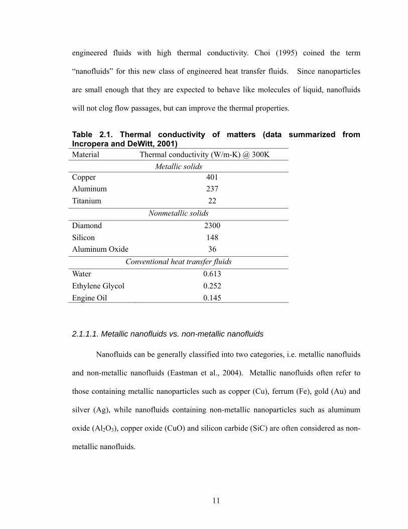
Generally, conventional heat transfer fluids have poor heat transfer properties

compared to solids. As shown in Table 2.1, most solids have orders of magnitude larger

thermal conductivities than those of conventional heat transfer fluids. Therefore, fluids

containing suspended solid particles are expected to display significant enhancement in

thermal conductivities relative to conventional heat transfer fluids.

Numerous theoretical and experimental studies of the effective thermal

conductivity of fluids containing particles have been conducted since Maxwell's

theoretical work was published more than 100 years ago. However, these studies were

confined to dispersions containing millimeter- or micrometer-sized particles. In

developing advanced fluids for industrial applications, it was identified that millimeter-

or micrometer-sized sized particles have severe clogging and abrasive problems.

With the development of nanopowder synthesizing techniques, it was proposed

that nanometer sized solid particles can be uniformly and stably suspended in industrial

heat transfer fluids such as water, ethylene glycol, or engine oil to produce a new class of

11

engineered fluids with high thermal conductivity. Choi (1995) coined the term

“nanofluids” for this new class of engineered heat transfer fluids. Since nanoparticles

are small enough that they are expected to behave like molecules of liquid, nanofluids

will not clog flow passages, but can improve the thermal properties.

Table 2.1. Thermal conductivity of matters (data summarized from Incropera and DeWitt, 2001) Material Thermal conductivity (W/m-K) @ 300K

Metallic solids Copper 401 Aluminum 237 Titanium 22

Nonmetallic solids Diamond 2300 Silicon 148 Aluminum Oxide 36

Conventional heat transfer fluids Water 0.613 Ethylene Glycol 0.252 Engine Oil 0.145

2.1.1.1. Metallic nanofluids vs. non-metallic nanofluids

Nanofluids can be generally classified into two categories, i.e. metallic nanofluids

and non-metallic nanofluids (Eastman et al., 2004). Metallic nanofluids often refer to

those containing metallic nanoparticles such as copper (Cu), ferrum (Fe), gold (Au) and

silver (Ag), while nanofluids containing non-metallic nanoparticles such as aluminum

oxide (Al2O3), copper oxide (CuO) and silicon carbide (SiC) are often considered as non-

metallic nanofluids.

12

2.1.1.2. Thermal conductivity of nanofluids

Conventional heat conduction models for solid-liquid mixtures have long been

established such as Maxwell model (Maxwell, 1904), Hamilton–Crosser model

(Hamilton and Crosser, 1962) and Jeffrey model (Jeffrey, 1973). However, these

conventional heat conduction models were confined to dispersions containing millimeter-

or micrometer-sized particles. When applying to nanofluids, they usually underestimate

the thermal conductivity (Wang et al., 1999; Choi, et al., 2001a; Jang and Choi, 2004).

Thus, thermal conductivity of nanofluids has been widely studied since 1993

(Masuda et al., 1993), although the term “nanofluids” was later on coined by Choi (1995).

Transient hot wire method is well developed to experimentally measure the thermal

conductivity of nanofluids (Nagasaka and Nagashima, 1981). Table 2.2 summaries the

literature review for thermal conductivity of nanofluids.

Metallic nanofluids have been widely studied. Choi et al. (2001a) found that the

effective thermal conductivity of ethylene glycol was improved by up to 40% through the

dispersion of 0.3 vol% Cu nanoparticles of 10 nm mean diameter, while Xuan and Li.

(2000) demonstrated that the effective thermal conductivity of water was increased by up

to 78% with 7.5 vol% Cu nanoparticles of 100 nm mean diameter. Hong et al. (2005)

reported that the thermal conductivity of Fe nanofluids is increased nonlinearly up to

18% as the volume fraction of particles is increased up to 0.55 vol%. Patel et al. (2003)

studied behavior of Au and Ag nanoparticles dispersed in water and found that the water

soluble Au nanoparticles, 10–20 nm in mean diameter, made with citrate stabilization

showed thermal conductivity enhancement of 5–21% in the temperature range of 30–

60ºC at a loading of 0.026 vol%, however, comparatively lower thermal conductivity

13

enhancement was observed for larger diameter Ag particles for higher loading (average

diameter of 60-80 nm).

Non-metallic nanofluids such as Al2O3, CuO, SiC, TiO2 and carbon nanotubes

also have been studied. The early research work by Masuda et al. (1993) reported 30%

increases in the thermal conductivity of water with the addition of 4.3 vol% Al2O3

nanoparticles (average diameter of 13 nm). A subsequent study by Lee et al. (1999),

however, observed only a 15% enhancement in thermal conductivity at the same

nanoparticle loading (average diameter of 33 nm). Xie et al. (2002a) found an

intermediate result, that is, the thermal conductivity of water is enhanced by

approximately 21% by a nanoparticle loading of 5 vol% (average diameter of 68 nm).

These differences in behavior were probably attributed to differences in average particle

size in the samples. Nanofluids consisting of CuO nanoparticles dispersed in water and

ethylene glycol seem to have larger enhancements in thermal conductivity than those

containing Al2O3 nanoparticles (Lee et al., 1999). The early research by Eastman et al.

(1997) showed that increase in thermal conductivity of approximately 60% can be

obtained for the nanofluid consisting of water and 5 vol% CuO nanoparticles with

average grain size of 36 nm. While Lee et al. (1999) observed only a modest

improvement of nanofluids containing CuO compared with those containing Al2O3,

Zhou and Wang (2002) observed a 17% increase in thermal conductivity for a loading of

only 0.4 vol% CuO nanoparticles in water. Xie et al. (2002b) studied SiC (average

diameter of 26 nm) in water suspension and reported that the thermal conductivity can be

increased by about 15.8% at 4.2 vol%. Murshed et al. (2005) showed that the measured

thermal conductivity for water based TiO2 nanofluids (average diameter of 15 nm) has a

14

maximum enhancement 30% for 5 vol% of particles.

Carbon nanotube nanofluids, is of special interests to researchers because of the

novel properties of carbon nanotubes -extraordinary strength, unique electrical properties,

and efficient conductors of heat. Carbon nanotubes (CNTs) are fullerene-related

structures that consist of either a grapheme cylinder (the so-called single-wall carbon

nanotubes, SWCNTs) or a number of concentric cylinders (the so-called multiwalled

carbon nanotubes, MWCNTs) (Wen and Ding, 2004b). Choi et al. (2001b) measured the

effective thermal conductivity of MWCNTs dispersed in synthetic (poly-α-olefin) oil and

reported the enhancement up to a 150% in conductivity at approximately 1 vol% CNT,

which is by far the highest thermal conductivity enhancement ever achieved in a liquid

(Lockwood et al., 2005). However, this huge enhancement was not observed by Xie et al.

(2003) for water/ ethylene glycol/decene based MWCNTs nanofluids, nor by Assael et al.

(2004) for water based MWCNTs nanofluids. The maximum thermal conductivity

enhancements observed by Xie et al. (2003) are 19.6%, 12.7%, and 7.0% for MWCNTs

suspension at 1.0 vol% in decene, ethylene glycol, and water, respectively, and that

observed by Assael et al. (2004) was 38% for MWCNTs suspension at 0.6 vol% in water.

As shown in Table 2.2, the reported measurement results are not very consistent.

This is probably because different researchers may have different experimental procedure

and there is uncertainty in the thermal conductivity measurement using hot wire method.

2.1.1.3. Particle size dependent thermal conductivity of nanofluids

There has not been a systematic experimental investigation of size-dependent

conductivity reported (Jang and Choi, 2004). However, Wang et al. (1999) compared

15

their experimental data with those of other investigators, and concluded it is possible that

the thermal conductivity of nanoparticle fluid mixtures increases with the decreasing

particle size. How the particle size affect the thermal conductivity of nanofluids will be

studied in our research.

Table 2.2. Summary of literature review for thermal conductivity of nanofluids

Particle Base fluid

Average particle

size

Volume fraction

Thermal conductivity enhancement

Reference

Cu Ethylene glycol 10 nm 0.3% 40% Choi et al.

(2001a)

Cu Water 100 nm 7.5% 78% Xuan and Li (2000)

Fe Ethylene glycol 10 nm 0.55% 18% Hong et al.

(2005)

Au Water 10–20 nm 0.026% 21% Patel et al. (2003) M

etal

lic n

anof

luid

s

Ag Water 60-80 nm 0.001% 17% Patel et al. (2003)

Al2O3 Water 13 nm 4.3% 30% Masuda et al. (1993)

Al2O3 Water 33 nm 4.3% 15% Lee et al. (1999)

Al2O3 Water 68 nm 5% 21% Xie et al. (2002a)

CuO Water 36 nm 5% 60% Eastman et al. (1997)

CuO Water 36 nm 3.4% 12% Lee et al. (1999)

CuO Water 50 nm 0.4% 17% Zhou and Wang (2002)

SiC Water 26 nm 4.2% 16% Xie et al. (2002b)

TiO2 Water 15 nm 5% 30% Murshed et al. (2005)

MWCNT(1) Synthetic oil

25 nm in diameter 50 μm in

length

1% 150% Choi et al. (2001b)

MWCNT Decene/ Ethylene

glycol/ Water


length

1% 20%/13%/7% Xie et al. (2003)

Non

-met

allic

nan

oflu

ids

MWCNT Water


length

0.6% 38% Assael et al. (2004)

(1) MWCNT: multi-walled carbon nanotube

16

2.1.1.4. Temperature dependent thermal conductivity of nanofluids

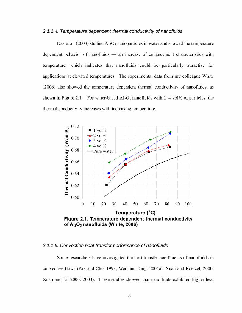
Das et al. (2003) studied Al2O3 nanoparticles in water and showed the temperature

dependent behavior of nanofluids — an increase of enhancement characteristics with

temperature, which indicates that nanofluids could be particularly attractive for

applications at elevated temperatures. The experimental data from my colleague White

(2006) also showed the temperature dependent thermal conductivity of nanofluids, as

shown in Figure 2.1. For water-based Al2O3 nanofluids with 1–4 vol% of particles, the

thermal conductivity increases with increasing temperature.

0.60

0.62

0.64

0.66

0.68

0.70

0.72

0 10 20 30 40 50 60 70 80 90 100

Temperature (oC)

The

rmal

Con

duct

ivity

(W

/m-K

) 1 vol%2 vol%3 vol%4 vol%Pure water

Figure 2.1. Temperature dependent thermal conductivity of Al2O3 nanofluids (White, 2006)

2.1.1.5. Convection heat transfer performance of nanofluids

Some researchers have investigated the heat transfer coefficients of nanofluids in

convective flows (Pak and Cho, 1998; Wen and Ding, 2004a ; Xuan and Roetzel, 2000;

Xuan and Li, 2000; 2003). These studies showed that nanofluids exhibited higher heat

17

transfer coefficient than base fluids, and the Nusselt number of nanofluids increased with

increasing volume fraction of the suspended nanoparticles and the Reynolds number.

Nanofluids are multicomponent systems, and the morphology and orientation of

the dispersed solids is complex (Yang et al., 2005). Experimental data have shown that

both classical correlations, Shah equation (for laminar flows) and Dittus–Boelter equation

(for turbulent flows) fail to predict convection heat transfer behavior of nanofluids (Wen

and Ding, 2004a ; Xuan and Li, 2003). Currently, there are very few correlations

developed for convection heat transfer coefficients of nanofluids (Xuan and Li, 2000;

2003).

Wen and Ding (2004a) studied convective heat transfer of nanofluids made of

Al2O3 nanoparticles and water in the laminar flow regime, and showed that for nanofluids

containing 1.6 vol% Al2O3 nanoparticles the local heat transfer coefficient was increased

by 15 – 45% (depending on the distance from entrance region). Xuan and Li (2000; 2003)

measured the convective heat transfer coefficient of nanofluids for turbulent flow and

found that compared with water, the Nusselt number was increased more than 39% for

the nanofluids with 2.0 vol% of Cu nanoparticles.

2.1.2. Nanofluid for Lubrication Application

On the other hand, as we know, solid lubricants are useful for conditions when

conventional liquid lubricants are inadequate such as high temperature and extreme

contact pressures. Their lubricating properties are attributed to a layered structure on the

molecular level with weak bonding between layers. Such layers are able to slide relative

to each other with minimal applied force, thus giving them their low friction properties.

18

Graphite and molybdenum disulfide (MoS2) are the predominant materials used as solid

lubricant. Other useful solid lubricants include boron nitride, tungsten disulfide,

polytetrafluorethylene (PTFE), etc, as listed in Table 2.3.

To improve the tribological properties of lubricating oils by dispersing

nanoparticles, especially nanoparticulate solid lubricants, becomes of interest to people.

Recent research has shown that lubricating oils with nanoparticle additives exhibit

improved load-carrying capacity, anti-wear and friction-reduction properties. Xu et al.

(1996) investigated tribological properties of the two-phase lubricant of paraffin oil and

diamond nanoparticles, and the results showed that, under boundary lubricating

conditions, this kind of two-phase lubricant possesses excellent load-carrying capacity,

anti-wear and friction-reduction properties. According to Verma et al. (2007), MoS2 in its

nanoparticulate form has exceptional tribological properties, which can reduce friction

under extreme pressure conditions. Wu et al. (2006) examined the tribological properties

of lubricating oils with CuO, TiO2, and diamond nanoparticles additives. The

experimental results show that nanoparticles, especially CuO, added to standard oils

exhibit good friction-reduction and anti-wear properties.

Table 2.3. Solid lubricant (1)

Solid Lubricant Formula Temperature resistance (oxidizing atmosphere) (2)

Graphite C 450 ºC Molybdenum disulfide MoS2 400 ºC Boron nitride BN 1200 ºC Tungsten disulfide WS2 450 ºC PTFE -- 260 ºC (1)Reference: http://www.tribology-abc.com/sub15.htm (2)Temperature resistance is even higher in reducing/non-oxidizing environments (for example, MoS2 up to 1100°C)

19

2.2. Nanofluids Synthesis

2.2.1. Overview

There are three ways to fabricate nanofluids, two-step physical process (Choi et

al., 2001a), one-step physical process (Choi et al., 2001a; Choi and Eastman, 2001), and

one-step chemical process (Zhu et al., 2004).

2.2.1.1. Two-step physical process

Nanoparticles are first produced as a dry powder, typically by inert gas–

condensation, which involves the vaporization of a source material in a vacuum chamber

and subsequent condensation of the vapor into nanoparticles via collisions with a

controlled pressure of an inert gas such as helium. The resulting nanoparticles are then

dispersed into a fluid in a second processing step. An advantage of this technique in

terms of eventual commercialization of nanofluids is that the inert-gas condensation

technique has already been scaled up to economically produce tonnage quantities of

nanopowders (Wagener and Gunther, 1999).

2.2.1.2. One-step physical process

This technique synthesizes nanoparticles and disperses them into a fluid in a

single step. It was originally used to prepare extremely fine particles of Ag by vacuum

evaporation onto a running oil substrate, which was developed by Yatsuya and coworkers

(Yatsuya et al., 1978) and later improved by Wagener and coworkers (Wagener et al.,

1997; Wagener and Gunther, 1999). Choi and Eastman (2001) used this technology to

20

produce nanofluids. As shown in Figure 2.2 (Choi and Eastman, 2001), the technique

involves vaporization of a source material under vacuum conditions, and condensation of

the vapor occurs via contact between the vapor and a flowing liquid. Nanoparticle

agglomeration is minimized by flowing the liquid continuously, which results in good

dispersion. However, the one-step physical process is very expensive and at present the

volume of nanofluids that can be produced via this direct-evaporation technique is much

more limited than with two-step physical process because of the limited space in the

vacuum chamber (Eastman et al., 2004).

Cooling SystemLiquid

Resistively Heated Crucible

Figure 2.2. Schematic drawing of the one-step physical process (Choi and Eastman, 2001).

2.2.1.3. One-step chemical process

Zhu et al. (2004) developed a one-step chemical process for producing stable Cu

in ethylene glycol nanofluids by reducing copper sulfate pentahydrate (CuSO4·5H2O)

with sodium hypophosphite (NaH2PO2· H2O) in ethylene glycol under microwave

21

irradiation. The thermal conductivity enhancement approaches that of the Cu nanofluids

prepared by a one-step physical method. It is found to be a fast, efficient one-step

chemical method to prepare Cu nanofluids. However, this method is still in the research

stage and the types of nanofluids it can produce are limited. Thus, we will not use one-

step chemical process to produce nanofluids in our research.

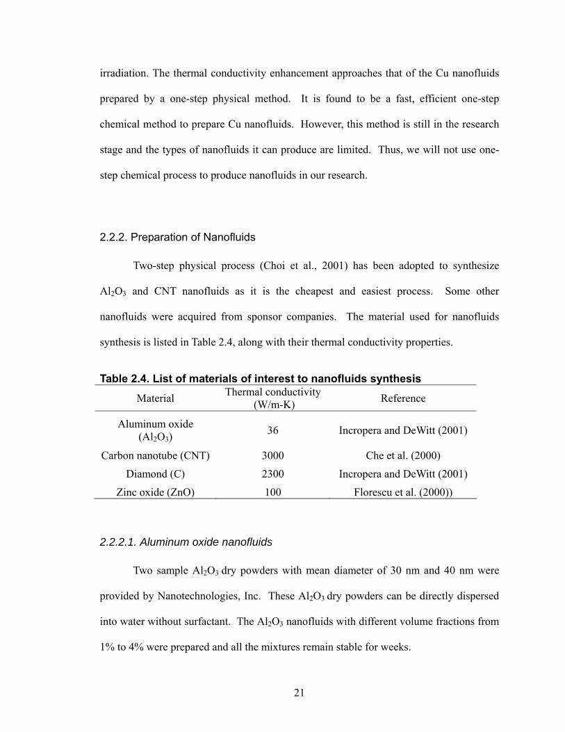
2.2.2. Preparation of Nanofluids

Two-step physical process (Choi et al., 2001) has been adopted to synthesize

Al2O3 and CNT nanofluids as it is the cheapest and easiest process. Some other

nanofluids were acquired from sponsor companies. The material used for nanofluids

synthesis is listed in Table 2.4, along with their thermal conductivity properties.

Table 2.4. List of materials of interest to nanofluids synthesis

Material Thermal conductivity (W/m-K) Reference

Aluminum oxide (Al2O3)

36 Incropera and DeWitt (2001)

Carbon nanotube (CNT) 3000 Che et al. (2000)

Diamond (C) 2300 Incropera and DeWitt (2001)

Zinc oxide (ZnO) 100 Florescu et al. (2000))

2.2.2.1. Aluminum oxide nanofluids

Two sample Al2O3 dry powders with mean diameter of 30 nm and 40 nm were

provided by Nanotechnologies, Inc. These Al2O3 dry powders can be directly dispersed

into water without surfactant. The Al2O3 nanofluids with different volume fractions from

1% to 4% were prepared and all the mixtures remain stable for weeks.

22

2.2.2.2. Carbon nanotube nanofluids

Four multi-wall carbon nanotubes (MWCNTs) samples were purchased from

Shenzhen Nanotech Port Co., China. The speciation of the MWCNTs is listed in Table

2.5.

Table 2.5. Specification of multi-wall carbon nanotubes Multi-wall carbon nanotubes Main range of external diameter Length

L-MWCNT-1020 10-20 nm 5-15 μm S-MWCNT-1020 10-20 nm 1-2 μm

L-MWCNT-60100 60-100 nm 5-15 μm S-MWCNT-60100 60-100 nm 1-2 μm

Carbon nanotubes (CNTs) as produced are usually entangled and not ready to be

dispersed into fluids. Therefore, chemical surfactant is needed to disperse CNTs. With

surfactant Sodium Dodecyl Sulfate (SDS) along with ultrosonic bathing, multi-wall

carbon nanotubes are being able to be dispersed in distilled water or ethylene glycol.

CNTs nanofluids with different volume fractions from 0.1% to 1% were prepared and all

the mixtures remain stable for weeks.

2.2.2.3. Diamond nanofluids

Two samples of diamond nanofluid were directly provided by Saint-Gobain. One

of them contains 100 nm mono-crystalline diamonds with no coating (Diamond nanofluid

#1) and the other contains 200 nm carbon outer coated diamonds (Diamond nanofluid #2).

Both samples have 1.5% volume fraction of diamonds. The fluid appears grey and

remains stable for weeks.

23

2.2.2.4. High volume fraction nanofluids

Six samples of water based nanofluid with high volume fraction were provided by

Nanophase Technologies (Romeoville, Illinois), as listed in Table 2.6. Three of the

samples contain Al2O3 nanoparticles with average particle sizes of 20, 46 and 80nm. The

other three contain ZnO nanoparticles with average particle sizes of 20, 40 and 60nm.

The stable high volume fraction dispersions were obtained by the addition of chemical

dispersants which is not disclosed by the company. As shown in the table, the volume

fraction of nanofluids ranges from 10.6% to 22.1%. These concentrations are

significantly higher than those of nanofluids studied in previous literature.

Table 2.6. List of nanofluids provided by Nanophase Molecular formulation Particle size Volume fraction

20 nm 10.6% 46 nm 21.7% Al2O3 80 nm 22.1% 20 nm 10.9% 40 nm 11.0% ZnO 60 nm 15.0%

2.3. Thermal Conductivity Measurements

The thermal conductivity of nanofluids were measured using transient hot wire

method, as described in Appendix A.1 in detail.

2.3.1. Aluminum Oxide Nanofluids

Al2O3 Al2O3fraction from 1% to 4% were prepared using two-step physical

process as described in Chapter 2. The thermal conductivity of these Al2O3 nanofluids

24

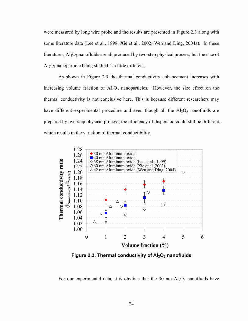
were measured by long wire probe and the results are presented in Figure 2.3 along with

some literature data (Lee et al., 1999; Xie et al., 2002; Wen and Ding, 2004a). In these

literatures, Al2O3 nanofluids are all produced by two-step physical process, but the size of

Al2O3 nanoparticle being studied is a little different.

As shown in Figure 2.3 the thermal conductivity enhancement increases with

increasing volume fraction of Al2O3 nanoparticles. However, the size effect on the

thermal conductivity is not conclusive here. This is because different researchers may

have different experimental procedure and even though all the Al2O3 nanofluids are

prepared by two-step physical process, the efficiency of dispersion could still be different,

which results in the variation of thermal conductibility.

1.001.021.041.061.081.101.121.141.161.181.201.221.241.261.28

0 1 2 3 4 5 6Volume fraction (%)

The

rmal

con

duct

ivity

rat

io(k

nano

fluid

s / k

wat

er)

30 nm Aluminum oxide40 nm Aluminum oxide38 nm Aluminum oxide (Lee et al., 1999)60 nm Aluminum oxide (Xie et al.,2002)42 nm Aluminum oxide (Wen and Ding, 2004)

Figure 2.3. Thermal conductivity of Al2O3 nanofluids

For our experimental data, it is obvious that the 30 nm Al2O3 nanofluids have

25

larger thermal conductivity enhancement than 40 nm ones. Only 4 vol% loading of

Al2O3 nanoparticles can increase the thermal conductivity by 17% for 30 nm particles

and 14% for 40 nm particles.

2.3.2. Diamond Nanofluids

Two diamond nanofluid samples received from Saint-Gobain (Warren/Amplex

Superabrasives were also tested. Both samples were formulated to have a volume

fraction of 1.5% diamond:

• Diamond nanofluid #1: 100 nm mono-crystalline diamond with no coating.

• Diamond nanofluid #2: 200 nm carbon outer coated diamond.

The thermal conductivity of both diamond nanofluid samples was measured by

short wire probe and the results are presented in Table 2.7. Diamond nanofluid # 1 has an

enhancement of 13% in thermal conductivity and diamond nanofluid # 2 has an

enhancement of 8%.

Table 2.7. Thermal conductivity measurement results of diamond nanofludis

Diamond nanofluid #1

Diamond nanofluid #2

Thermal conductivity (W/m-K) 0.687 0.657 Thermal conductivity enhancement (relative to deionized water) 13% 8%

2.3.3. Carbon Nanotube Nanofluids

Stable multi-wall carbon nanotubes (MWCNT) suspension in pure water was

obtained using 0.1 wt% sodium dodecyl sulfate (SDS) as surfactant and subjected to 30

26

min of ultrasonic homogenization, as described in Chapter. The test nanotubes were

purchased from Shenzhen Nanotech Port Co., which has mean diameter of 10-20 nm and

length of 5-15 μm. Thermal conductivities at different volume fraction were measured by

short-wire probe. However, as shown in Figure 2.4, the thermal conductivity

enhancements are only 1.9%, 2.5%, and 3.4%, respectively for the volume fraction of

0.2%, 0.4%, and 0.6%, which is not as high as expected. This is probably attributed to

the dispersion method as well as the quality of nanotubes.

1.000

1.005

1.010

1.015

1.020

1.025

1.030

1.035

1.040

1.045

1.050

0 0.2 0.4 0.6 0.8Volume fraction (%)

Ther

mal

con

duct

ivity

ratio

(K

nano

fluid

s / K

wat

er)

Figure 2.4. Thermal conductivity of MWCNT nanofluids

2.3.4. High Volume Fraction Nanofluids

Six samples of high volume fraction nanofluids are provided by Nanophase, as

discussed in Section 2.2.2. Nanofluids with various volume fractions can be further

obtained by dilution with deionized water.

27

The thermal conductivity measurement of water-based Al2O3 nanofluids with

particle sizes of 20, 46, and 80 nm is shown in Figure 2.5. The thermal conductivity

enhancement increases with increasing volume fraction of nanoparticles. The

improvement of thermal conductivity reaches 43% with 22 vol% of 80 nm Al2O3

nanoparticles. It also indicates that the larger particle size has larger enhancement in

thermal conductivity.

1.00

1.05

1.10

1.15

1.20

1.25

1.30

1.35

1.40

1.45

1.50

0% 5% 10% 15% 20% 25%

Volume fraction

k nan

oflu

ids/k

wat

er

20nm aluminum oxide nanofluid46nm aluminum oxide nanofluid80nm aluminum oxide nanofluid

Figure 2.5. Thermal conductivity of high volume fraction Al2O3 nanofluids

The thermal conductivity of water-based ZnO nanofluids with particle sizes of 20,

40, and 60 nm was also characterized and plotted in Figure 2.6. The results are very

similar to those of Al2O3 nanofluids. The thermal conductivity enhancement increases

with increasing volume fraction of nanoparticles, as well as the increasing particle size.

For the ZnO nanofluid with a particle size of 60 nm, the increase in thermal conductivity

is about 61% at the 15 vol%.

28

In addition, the experimental results indicated that the ZnO nanofluids have better

thermal conductivity improvement than Al2O3 nanofluids. This is probably because the

thermal conductivity of ZnO is about three times higher than that of Al2O3.

1.00

1.10

1.20

1.30

1.40

1.50

1.60

1.70

1.80

0% 5% 10% 15% 20%Volume fraction

k nan

oflu

ids/k

wat

er

20nm ZnO nanofluid

40nm ZnO nanofluid

60nm ZnO nanofluid

Figure 2.6. Thermal conductivity of high volume fraction ZnO nanofluids

Thermal conductivity is a critical to the heat conduction, but when it comes to the

cooling application of fluids, convection becomes more of significant. Moreover, since

there is increasing demand for more efficient microchannel cooling in microelectronics

and fuel cell application, it is necessary to study cooling behavior of nanofluids in

microchannels. Therefore, convection heat transfer of nanofluids in microchannels was

investigated in this research.

29

2.4. Convection Heat Transfer Coefficient Measurements

The internal pipe flow convection coefficient of nanofluids was measured

experimentally. The principle, experimental setup and the calibration can be found in

Appendix A.2.

The water-based Al2O3 nanofluid from Nanophase was diluted to various volume

fractions for convection heat transfer coefficient study. The suspended Al2O3 particle has

an average size of 46 nm. The high volume fraction results in the high viscosity of the

fluid and a tendency for the nanoparticles to stick on the walls of tubing and containers.

It also requires large pumping power. Therefore, the highest concentration of the testing

fluid in this study was 5 vol%. The thermal conductivity of these testing fluids were

measured and summarized in Table 2.8.

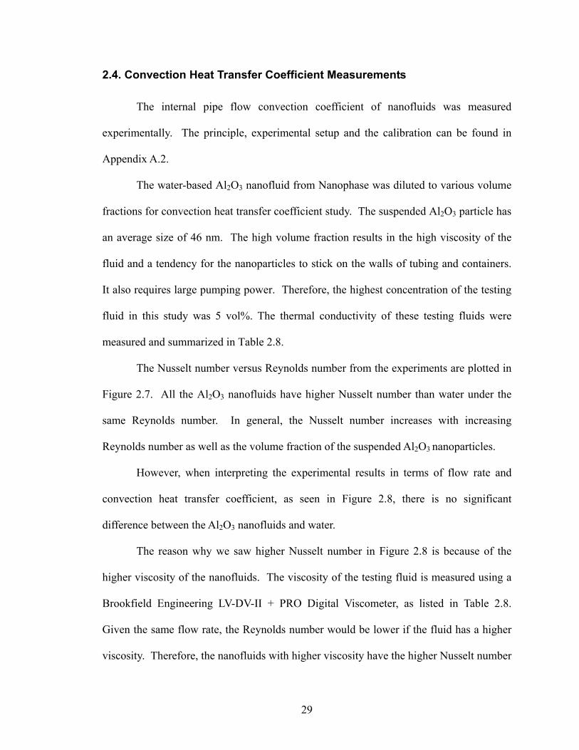
The Nusselt number versus Reynolds number from the experiments are plotted in

Figure 2.7. All the Al2O3 nanofluids have higher Nusselt number than water under the

same Reynolds number. In general, the Nusselt number increases with increasing

Reynolds number as well as the volume fraction of the suspended Al2O3 nanoparticles.

However, when interpreting the experimental results in terms of flow rate and

convection heat transfer coefficient, as seen in Figure 2.8, there is no significant

difference between the Al2O3 nanofluids and water.

The reason why we saw higher Nusselt number in Figure 2.8 is because of the

higher viscosity of the nanofluids. The viscosity of the testing fluid is measured using a

Brookfield Engineering LV-DV-II + PRO Digital Viscometer, as listed in Table 2.8.

Given the same flow rate, the Reynolds number would be lower if the fluid has a higher

viscosity. Therefore, the nanofluids with higher viscosity have the higher Nusselt number

30

under the same Reynolds number, which is actually corresponding to a higher flow rate.

40

90

140

190

240

290

0 3,000 6,000 9,000 12,000 15,000Re

Nu

Water1 vol% aluminum oxide3 vol% aluminum oxide5 vol% aluminum oxide

Figure 2.7. Nusselt number versus Reynolds number

0

50,000

100,000

150,000

200,000

250,000

0 200 400 600 800

Flow rate (ml/min)

h (W

/m2 -K

)

Water1 vol% aluminum oxide3 vol% aluminum oxide5 vol% aluminum oxide

Figure 2.8. Convection heat transfer coefficient flow rate

31

Table 2.8. Physical properties of testing fluids (room temperature)

Fluid Volume Fraction

Thermal Conductivity

(W/m-K)

Density (kg/m3)

Viscosity (Ns/m2)

Water -- 0.61 997 8.55×10-4 1% 0.62 1030 1.30×10-3 3% 0.63 1080 1.50×10-3

Al2O3 nanofluids (NanoDur X1121W)

5% 0.66 1130 2.04×10-3

2.5. Concluding Remarks

Two-step physical process was used to synthesize nanofluids containing Al2O3

nanoparticles and multi-wall carbon nanotubes. Diamond nanofluids and high volume

fraction nanofluids were also acquired from Saint-Gobain Warren Amplex Superabrasives

and Nanophase, respectively.

Both the long and short hot wire probes were developed to measure the thermal

conductivity of nanofluids based on transient hot wire method. For Al2O3 nanofluids, the

thermal conductivity enhancement increases with increasing volume fraction of

nanoparticles. Only 4 vol% loading of Al2O3 nanoparticles can increase the thermal

conductivity by 17% for 30 nm particles and 14% for 40 nm particles. Diamond

nanofluids also show some enhancement in thermal conductivity (13% for 100 nm

diamond particles and 8% for 200 nm diamond particles at 1.5 vol%). However, carbon

nanotube nanofluids only have little enhancement in thermal conductivity. This is

probably attributed to the dispersion method as well as the quality of nanotubes. High

volume fraction water-based Al2O3/ZnO nanofluids were also tested. Much higher

thermal conductivity enhancement of 61% was observed for ZnO nanofluids at 15 vol%.

The convection heat transfer coefficient measurement apparatus was also

32

developed. The calibration was conducted on pure water and the results are consistent

with the literature. The water-based Al2O3 nanofluid (average particle size of 46 nm) of

various volume fractions was used for convection heat transfer study. The nanofluids

showed higher Nusselt number than its base fluid at the same Reynolds number; however,

in terms of convection heat transfer coefficient vs. flow rate, there is no significant

difference between the nanofluids and the base fluid. The increase in Nusselt number of

nanofluids is mainly due to the higher viscosity, compared to the base fluid.

33

CHAPTER 3

MINIMUM QUANTITY LUBRICATION (MQL) GRINDING USING

NANOFLUIDS

MQL grinding (conventional abrasive wheels) of cast iron using water based and

oil based nanofluids was investigated. Grinding performance is evaluated and compared

in terms of grinding force, G-ratio, and surface roughness, etc.

Water-based Al2O3 and diamond nanofluids were applied in MQL grinding

process and the grinding results were compared with those of pure water. During the

nanofluid MQL grinding, a dense and hard slurry layer was formed on the wheel surface

and could benefit the grinding performance. Experimental results showed that G-ratio,

defined as the volume of material removed per unit volume of grinding wheel wear, could

be improved with high concentration nanofluids. However, water based nanofluids are

not able to provide superior cooling capacity in MQL grinding process. Thus, the

research of MQL grinding using nanofluids focuses on the advanced lubrication

properties hereafter.

Oil-based nanofluids were also applied in MQL grinding. Active MoS2

nanoparticles were added in low and high concentrations, to three commercially available

34

base oils. To test value addition due to nanoparticles, their MQL grinding performances

were compared with that of the pure base oils (without MoS2 nanoparticles) and with

regular water based grinding fluid using flood cooling (wet) application. The results

showed that lubricants with novel MoS2 nanoparticles significantly reduces the tangential

grinding force and friction between the wear flats and the workpiece, increases G-ratio

and improves the overall grinding performance in MQL applications.

3.1. Background

Grinding is widely used as the finishing machining process for components that

require smooth surfaces and precise tolerances. Large fluid delivery and cooling systems

are evident in production plants. As mentioned in Chapter 1, from both environmental

and economical points of view, there are critical needs to reduce the use of cutting fluid

in grinding process, and MQL grinding is a promising solution.

MQL grinding using conventional abrasive wheel has been investigated

(Brinksmeier et al., 1997; Baheti et al., 1998; Hafenbraedl and Malkin, 2000), and it was

concluded that MQL has shortcomings of insufficient workpiece cooling with

conventional abrasives.

The fluid and the grinding wheel are the key technical areas that can enable the

success of MQL grinding processes. The advanced heat transfer and tribological

properties of nanofluids may provide better cooling and lubricating in the MQL grinding

process, and make it production-feasible.

35

3.2. MQL Grinding using Water Based Nanofluids

3.2.1. Experimental Setup

The grinding experiments were conducted in an instrumented Chevalier Model

Smart-B818 surface grinding machine. The setup of the grinding experiment is shown in

Figure 3.1. A vitreous bond aluminum oxide grinding wheel (Saint-Gobain/Norton

32A46-HVBEP) with 508 µm average abrasive size was used. The initial diameter and

the width of wheel were 177.8 mm and 12.7 mm, respectively. The workpiece material

was Dura-Bar 100-70-02 ductile iron with a carbon content of 3.5-3.9% and hardness of

50 Rockwell C. The width and length of the workpiece surface for grinding are 6.5 mm

and 57.5 mm, respectively. MQL grinding utilized a special fluid application system

shown in Figure 3.1(b) provided by AMCOL (Hazel Park, Michigan). In this system,

biaxial hose is used to independently transport liquid and air to the point of use and then

the liquid is surrounded with air (coaxial) and propelled onto the tool or workpiece by air

pulse. For flood cooling, Cimtech 500 synthetic grinding fluid at 5 vol% concentration

was used and the flow rate was measured 5400 ml/min. For MQL grinding, the flow rate

was set to 5 ml/min for all grinding fluids including water-based nanofluids.

The surface grinding parameters were kept constant throughout the experiment –

30 m/s wheel surface speed, 10 μm depth of cut and 2400 mm/min workpiece velocity

(feed rate). Before every test, the grinding wheel was dressed at 10 μm down feed, 500

mm/min traverse speed and −0.4 speed ratio using a rotary diamond disk with 96 mm

diameter and 3.8 mm width.

The normal and tangential grinding forces were measured using a Kistler Model

9257A piezoelectric dynamometer. The grinding temperatures were measured by the

36

embedded thermocouple method (Shen et al., 2009), which will be discussed in detail in

Chapter 4. After each grinding pass, the workpiece was allowed to cool to the initial

temperature before the next pass was taken. The wheel wear measurement method is the

same as described in (Shih et al., 2003). The wheel was 12.7 mm wide. The width of the

part was narrower, 6.5 mm. A worn groove was generated on the wheel surface after

grinding. A hard plastic part was ground to produce a replica of the worn grinding wheel.

A Taylor Hobson Taylorsurf profilometer was used to measure the depth of wheel wear

on the replica. Each G-ratio grinding test had to wear out at least 6 μm of the wheel to

ensure the accuracy of G-ratio. The same profilometer was used to measure the surface

roughness of ground surfaces. Three measurement traces parallel and perpendicular to

the grinding direction were measured. The average of the three arithmetic average

surface roughness (Ra) measurements along and across the grinding direction was used to

represent the roughness of a ground surface.

(a) (b) Figure 3.1. Experimental setup: (a) Experiment layout and (b) MQL fluid delivery device

To air pipe

To air and liquid hoses

Fluid reservoir

Workpiece

Air hose

Liquid hose

37

3.2.2. Grinding Fluids

Four types of fluids were used in grinding tests, water-based Cimtech 500

(Milacron, Cincinnati, OH) synthetic grinding fluid at 5 vol% concentration, pure water,

water-based Al2O3 nanofluids, and water-based diamond nanofluids. The Al2O3

nanofluids were prepared by dispersing 40 nm Al2O3 nanoparticles (NovaCentrix, Austin,

Texas) to the deionized water. Three volume fractions of Al2O3 nanofluids at 1.0%, 2.5%

and 4.0% were tested. The 4.0 vol% is already on the high side of concentration for

Al2O3 nanofluids because of the noted increase in viscosity. Two diamond nanofluids

samples are provided by Warren/Amplex Superabrasives of Saint-Gobain. Both samples

are formulated to have weight fraction of 250 carats/1000 ml, which have an equivalent

volume fraction of 1.5% diamond. One sample contains 200 nm carbon coated diamonds

and the other contains 100 nm non-coated mono-crystalline diamonds.

Table 3.1. Fluid thermal conductivity

Fluids Thermal conductivity (W/m-K)

Thermal conductivity enhancement

Deionized water 0.603 -- Cimtech 500 synthetic fluid (5 vol%) 0.593 --

1.0 vol% 0.645 7% 2.5 vol% 0.670 11% Al2O3 nanofluids (40 nm diameter) 4.0 vol% 0.693 5%

Diamond nanofluids (200 nm carbon coated) 0.654 6%

Diamond nanofluids (100 nm non-coated )

1.5 vol% 0.684 10%

The thermal conductivity of fluids involved are all measured at room temperature

using transient hot wire method as described in Chapter 3. The results are summarized in

Table 3.1. All the nanofluids show some enhancement in thermal conductivity. Al2O3

38

nanofluids have thermal conductivity enhancement of 7%, 11% and 15% for 1.0%, 2.5%

and 4.0% volume fraction concentration, respectively. Diamond nanofluids at 1.5 vol%

have thermal conductivity enhancement of 6% for 200 nm carbon coated diamond and

10% for 100 nm non-coated diamond. The 5% concentration Cimtech 500 synthetic

grinding fluid causes the thermal conductivity drop to 0.593 W/m-K.

3.2.3. Grinding Forces

The specific grinding forces, which is defined as the forces divided by the width

of grinding, vs. passes are shown in Figures 3.2 and 3.3. These forces are the average

values in each grinding pass. The grinding forces for every 5 passes are plotted. As

shown in Figure 3.2, flood cooling and MQL grinding using Cimtech 500 generate

similar normal and tangential forces during the entire process. These forces are lower

than MQL grinding using pure water, which is expected because of the better lubricating

properties of Cimtech 500 cutting fluid. Dry grinding without lubrication generates the

highest forces. On the other hand, the forces increase with the number of passes, which

contributes to the wheel wear. Notice that the forces for dry grinding increase

exponentially after 110 passes. These large forces generate excessive heat and lead to

visible burning of the workpiece, which can be identified by discoloration on the ground

workpiece surface.

MQL grinding force results using pure water (considered as the datum) and water

based nanofluids are compared in Figure 3.3. In the beginning (before 35 passes), all the

forces are comparable. With increasing passes, MQL grinding using different fluids

exhibit different performance. For Al2O3 nanofluids, at 1.0 vol% low concentration, the

39

grinding forces increase progressively which is similar to the case of pure water. At

higher concentration (2.5 and 4.0 vol%), the grinding forces remain flat after increasing

in the beginning. This may be due to the hard and dense slurry layer observed on the

grinding wheel. However, compared with Al2O3 nanofluid of 2.5 vol%, the one with 4.0

vol% gives much higher forces. The possible explation is that the high concentration of

Al2O3 (4.0 vol%) leads to excessive loading of the vitreous bond grinding wheel,

resulting in higher grinding forces.

For diamond nanofluids, the grinding forces become flat after about 45 passes.

Again, the slurry layer is readily observed when using 200 nm carbon coated diamond

nanofluids, but not for 100 nm non-coated diamond nanofluids. Intense loading on the

wheel is likely why the grinding forces are higher with 200 nm carbon coated diamond

nanofluid than with 100 nm non-coated diamond nanofluid. In general, the slurry layer

can reduce the grinding forces by reducing the wheel wear, which is supported by the G-

ratio measurement results.

The force ratio Ft /Fn indicates the combination of abrasive cutting and friction

between the wear flats and the workpiece. In all the experiments, this ratio decreases

from the beginning and then reaches a relatively steady state value. As shown in Figure

3.2, the force ratio is 0.15 for dry, 0.2 for pure water and Cimtech 500 MQL, and 0.25 for

Cimtech 500 flood cooling grinding. For nanofluid MQL grinding, as shown in Figure

3.3, the force ratio is 0.25 for all three Al2O3 based nanofluids and about 0.27 and 0.2 for

the 100 and 200 nm diamond nanofluids grinding, respectively. The initial drop is

probably due to the rise of workpiece temperature during grinding. In dry grinding, the

ratio is very low, which is attributed to the workpiece burning and associated phase

40

changes (Malkin, 1989).

4

7

10

13

16

19

22

25

28Sp

ec. N

orm

al F

orce

, Fn

(N/m

m)

Pure Water MQLDryCimtech 500 (5%) MQLCimtech 500 (5%) Flood Cooling

1.2

1.6

2.0

2.4

2.8

3.2

3.6

4.0

Spec

. Tan

gent

ial F

orce

, Ft (

N/m

m)

0.10

0.15

0.20

0.25

0.30

0.35

0.40

5 35 65 95 125Passes

F t /

F n

4

6

8

10

12

14

16

18

Spec

. Nor

mal

For

ce, F

n (N

/mm

)

Pure Water MQL40 nm Aluminium Oxide (1%)40 nm Aluminium Oxide (2.5%)40 nm Aluminium Oxide (4%)100 nm Diamond (1.5%)200 nm Diamond (1.5%)

1.0

1.5

2.0

2.5

3.0

3.5

Spec

. Tan

gent

ial F

orce

, Ft (

N/m

m)

0.10

0.15

0.20

0.25

0.30

0.35

0.40

5 35 65 95 125Passes

F t /

F n

Figure 3.2. Specific grinding forces and force ratio for wet, dry and MQL grinding using Cimtech 500 and pure water

Figure 3.3. Specific grinding forces and force ratio for water based nanofluids MQL grinding

41

The specific tangential versus specific normal force for all grinding conditions are

illustrated in Figure 3.4. For given grinding conditions, a plot of tangential versus normal

force component per unit width should yield a straight line with a slope equal to the

friction coefficient between the wear flats and the workpiece. According to Malkin’s

analysis (Malkin, 1989), above the burn limit, the slope gets steeper which suggests a

decrease in friction coefficient associated with workpiece burn. The phase changes and

the formation of oxides on cast iron workpiece cause the reduction in friction coefficient.

This change in slope or friction coefficient is also observed in this study. As shown in

Figure 3.4, the specific tangential grinding force of about 2.2 N/mm is the transition point

for grinding burn and change of slope. This corresponds to a specific energy of 165

J/mm3, which is a little higher than 135 J/mm3 burning limit for low carbon and low alloy

steels (Malkin, 1989).

Linear curve fitting was applied to data points above and below 2.2 N/mm

specific tangential grinding force. In the absence of workpiece burn, below the specific

tangential grinding force of 2.2 N/mm, the slope is 0.33, which implies a friction

coefficient of 0.33 between the wear flats and the workpiece. With grinding burn, the

slope is much lower, 0.09. This indicates a much smaller friction coefficient beyond this

grinding burn point. This observation is consistent with the findings in previous grinding

studies (Malkin, 1989). Workpiece burning, evidenced by visible discoloration, is

apparent in three grinding conditions: dry, pure water MQL, and 1.0 vol% Al2O3

nanofluids MQL grinding. For dry grinding, except for several initial passes, most of the

data points are above the burn limit. This has also been observed on the discoloration of

the ground surface. In dry grinding the first few passes has no discoloration. After that,

42

severe discoloration was observed. The experimental observations of discoloration match

to the burn limit prediction in Figure 3.4. Slight discoloration was observed for pure

water and 1.0 vol% Al2O3 nanofluids MQL grinding. As shown in Figure 3.4, some data

from these experiments also locate above the burn limit. For pure water, the lack of

lubricity contributes to the workpiece burning. For 1.0 vol% Al2O3 nanofluid, it is likely

attributed to the relatively high grinding force than the other nanofluids, as shown in

Figure 3.3. No burning marks were observed for 2.5 vol% Al2O3 nanofluids, diamond

nanofluids, flood cooling, and MQL grinding with Cimtech 500 as the specific tangential

forces in these experiments are all below 2.2 N/mm.

Slope = 0.33

Slope = 0.09

1.0

1.5

2.0

2.5

3.0

3.5

4.0

4 8 12 16 20 24 28Spec. Normal Force, F n (N/mm)

Spe

c. T

ange

ntia

l For

ce, F

t (N

/mm

)

Cimtech 500 (5%) Flood cooling DryCimtech 500 (5%) MQL Pure Water MQL40 nm Aluminium Oxide (1%) 100 nm Diamond (1.5%)40 nm Aluminium Oxide (2.5%) 200 nm Diamond (1.5%)40 nm Aluminium Oxide (4%)

Workpiece burning

Figure 3.4. Specific tangential force vs. specific normal force

43

3.2.4. G-ratio

G-ratio is defined as the volume of work-material removed divided by the volume

of wheel wear. A high G-ratio indicates low wheel wear rate. Nanofluid MQL grinding

generally exhibits the high G-ratio, ranging from 16 to 33, as shown in Figure 3.5. Flood

cooling and MQL grinding using Cimtech 500 provides similar G-ratio, about 17. Dry

grinding exhibits the worst wheel wear, i.e., the lowest G-ratio, about 12, while MQL

using pure water has only a slightly higher G-ratio than that of dry grinding.

0

4

8

12

16

20

24

28

32

36

G-ra

tio

40 nm Al2O3

(1%)

Purewater

100 nm Diamond (1.5%)

Dry200 nm Diamond (1.5%)

40 nm Al2O3

(2.5%)

40 nm Al2O3

(4%)

Flood cooling

Cimtech 500(5%)

MQL grinding

Nanofluid MQL

Figure 3.5. G-ratio results

For MQL grinding with Al2O3 nanofluids, the G-ratio increases with increasing

volume fraction of Al2O3 nanoparticles. The two highest G-ratio results are observed in

MQL grinding with 2.5 and 4.0 vol% Al2O3 nanofluids. This is attributed to the

formation of the slurry layer which can protect the grinding wheel from grain/bond

44

fracture. High concentration nanofluid has better protection and improves the G-ratio.

The slurry layer is not observed in MQL grinding with 1.0 vol% Al2O3 nanofluid, which

has a low G-ratio. In early research (Komanduri and Reed, 1980), it was found that a thin

slurry layer of silicon carbide on the wheel surface can protect the bonding material from

thermal and/or mechanical degradation or damage, thereby causing a high G-ratio. This

research further validates this observation.

For MQL grinding with diamond, the same phenomenon of slurry formation and

high G-ratio was observed in the 200 nm diamond nanofluid. For the 100 nm diamond

nanofluid, no slurry layer was observed and the G-ratio is lower than that of the 200 nm

diamond nanofluids. Compared to the 100 nm diamond nanofluid, it should also be noted

that the 200 nm diamond nanofluid is more viscous and more readily to form the slurry

layer.

3.2.5. Surface Roughness

The surface roughness (Ra) of the ground workpiece are presented in Figure 3.6.

Flood cooling has the best surface finish (lowest surface roughness). In general, MQL

grinding using nanofluids has better surface finish than pure water but worse than the

flood cooling and MQL grinding using Cimtech 500. Cimtech 500 synthetic grinding

fluid provides good lubrication, while pure water has poor lubricating capability. The

flood cooling also provides efficient chip flushing. The fact that the nanofluids

outperform the pure water can be partly due to the reduction in grinding forces and

friction. Dry grinding has the worst surface finish, which is expected.

For Al2O3 nanofluids, 2.5 vol% has better surface roughness than that of 1.0 and

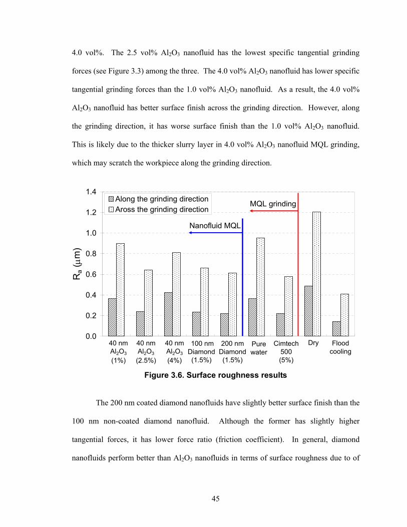
45

4.0 vol%. The 2.5 vol% Al2O3 nanofluid has the lowest specific tangential grinding

forces (see Figure 3.3) among the three. The 4.0 vol% Al2O3 nanofluid has lower specific

tangential grinding forces than the 1.0 vol% Al2O3 nanofluid. As a result, the 4.0 vol%

Al2O3 nanofluid has better surface finish across the grinding direction. However, along

the grinding direction, it has worse surface finish than the 1.0 vol% Al2O3 nanofluid.

This is likely due to the thicker slurry layer in 4.0 vol% Al2O3 nanofluid MQL grinding,

which may scratch the workpiece along the grinding direction.

0.0

0.2

0.4

0.6

0.8

1.0

1.2

1.4

Ra (

μm)

Along the grinding directionAross the grinding direction

40 nm Al2O3

(1%)

Purewater

100 nm Diamond (1.5%)

Dry200 nm Diamond (1.5%)

40 nm Al2O3

(2.5%)

40 nm Al2O3

(4%)

Flood cooling

Cimtech 500(5%)

MQL grinding

Nanofluid MQL

Figure 3.6. Surface roughness results

The 200 nm coated diamond nanofluids have slightly better surface finish than the

100 nm non-coated diamond nanofluid. Although the former has slightly higher

tangential forces, it has lower force ratio (friction coefficient). In general, diamond

nanofluids perform better than Al2O3 nanofluids in terms of surface roughness due to of

46

the lower specific tangential grinding forces, as seen in Figure 3.3.

3.2.6. Grinding Temperature

The comparison of wet, dry, and MQL grinding temperature at the workpiece

surface was plotted in Figure 3.7. Flood cooling has the lowest temperature and dry

grinding has the highest, which is expected. In Figure 3.7, all the MQL grinding

experiments have the same flowrate (5 ml/min). By applying MQL, the peak temperature

is about 100-150°C lower than that in dry grinding. This is due to both cooling and

lubrication effects of the fluids provided by MQL, as lubrication reduces the cutting

forces and cutting energy, while convection heat transfer and/or boiling carries away

some of the heat.

There is no significant difference in grinding temperature among the experiments

using different types of fluids for MQL grinding. The Cimtech 500 synthetic grinding

fluid has slightly lower grinding temperature. This is probably attributed to the better

lubrication properties of Cimtech 500 synthetic grinding fluid. The 4.0 vol% aluminum

oxide nanofluids also has a slightly lower workpiece surface grinding temperature. This

is probably due to the dense slurry layer formed during grinding, which may cause more

heat to enter the grinding wheel rather than the workpiece.

47

0

100

200

300

400

500

600

0 0.2 0.4 0.6 0.8

Time (s)

Tem

pera

ture

rise

(o C)

DryMQL (Pure water)MQL (1.5 vol% 100 nm diamond)MQL (1.0 vol% aluminum oxide)MQL (4.0 vol% aluminum oxide)MQL (Cimtech 500 (5%))Flood cooling

595490510500455460110

Peak temperature rise (oC)

Figure 3.7. Comparison of wet, dry, and MQL grinding temperature at the workpiece surface (5 ml/min flowrate for MQL grinding)

3.2.7. Summary

Grinding of cast iron under different lubrication conditions was studied. Grinding

performance was investigated and compared in terms of grinding forces, G-ratio, and

surface roughness. Dispersion of solid particles was found to play an important role,

48

especially when a slurry layer was formed. The slurry layer generated higher G-ratio

(less wheel wear), smaller grinding forces and better surface finish. To elucidate how the

slurry layer forms and how the dispersed solid particles and the slurry layer affect the

grinding performance, further research is needed.

The preliminary study of MQL grinding showed that it could significantly reduce

the grinding temperature compared to dry grinding. However, there is no significant

difference in grinding temperature when using nanofluids. This is probably because that

the amount of the nanofluids applied in MQL grinding is too small to make any

difference even though they have better thermal conductivity. In addition, convection is

probably the dominant cooling phenomenon for cutting fluids in grinding processes

rather than conduction. According to the previous convection heat transfer study of

nanofluids (Chapter 2), Al2O3 nanofluids virtually showed no improvement in the

convection heat transfer coefficient compared to the base fluid.

From above, it is concluded that nanofluids are not able to provide superior

cooling capacity in MQL grinding process. Therefore, the future research of application

of nanofluids in MQL grinding should focus on the advanced lubrication properties.

3.3. MQL Grinding using Oil Based Nanofluids

The core functionalities of cutting fluids are to cool and lubricate the grinding

zone. The water based fluids are used mainly where good cooling properties are required,

while the oil based fluids are used mainly where good lubricating property is a major

requirement.

Although the nanofluid has showed enhanced thermal conductivity, it was unable

49

to improve the convection heat transfer properties. The experimental results in the

previous section further confirmed that there is no advantage of applying nanofluids in

MQL grinding in terms of workpiece cooling (Shen et al., 2008a). On the other hand, the

suspension of nanoparticles can also improve the tribological properties of the base fluids,

which can help lubricate the grinding zone. Therefore, the oil based nanofluids with

advanced tribological properties are now considered for MQL grinding.

Molybdenum disulphide MoS2 is a predominant material used as solid lubricant,

due to their hexagonal closed pack (HCP) lamellar structure. The lamellas orient parallel

to the surface in the direction of motion (Wu et al. 2006). According to Verma et al. (2007)

and others, MoS2 in its nanoparticulate form has exceptional tribological properties,

showing that MoS2 nanostructured additive in paraffin oil reduces friction under extreme

pressure conditions. Malshe and Verma (2006) proposed for the first time that

nanoparticles of MoS2 suspended in the grinding fluid could navigate in the grinding

wheel – workpiece contact zone and provide significant lubrication.

In this section, MQL grinding performance of different lubricants with MoS2

nanoparticles additives was evaluated and compared with that of conventional flood

application.

3.3.1. Experimental Setup

The experimental setup is exactly the same as in Section 3.2.1, as is the grinding

parameter. The flow rate was selected at 5400 ml/min for flood cooling (wet) application

and 5 ml/min for MQL.

50

3.3.2. Grinding Fluids

For flood cooling application, water based synthetic grinding fluid Cimtech 500

(5 vol% concentration) was used. For MQL application, three commercially available

oils; namely: paraffin oil (mineral based oil), soybean oil (vegetable based oil) and

commercial MQL metal working fluid CANMIST (high purity fatty alcohol based oil,

AMCOL Corp.) were chosen as the base fluids, as listed in Table 3.2.

Table 3.2. Summary of base fluids Name Type Application

Cimtech 500 Water based synthetic grinding fluid (5 vol%) Flood Paraffin oil Mineral based MQL Soybean oil Vegetable based MQL

CANMIST oil High purity fatty alcohol based MQL

MoS2 nanoparticles based grinding lubricant additive consisted of molybdenum

disulphide nanoparticles (<100nm) intercalated with triglyceride chemistry plus

emulsifier (Alcolec) lecithin. This additive was dispensed in the three base oils. These

control media were selected based upon published literature and authors’ prior experience.

Soybean and paraffin oil is used as base oil in a number of commercially available

grinding fluids, for example, “Tru Cut 203NC” a paraffin oil based grinding fluid and

“ELM SoyEasy UNI-Cut™”, a soybean oil based grinding fluid.

To prepare the described nanoengineered molybdenum disulphide additive

(Malshe et al., 2006), first, MoS2 in powder form (Alfa Aesar, 98% pure, 3-5 µm average

particle size) was ball milled in SPEX 8000D mixer mills using hardened steel vials (with

a constant ball to powder ratio of 2:1) for 48 hours. This dry milled MoS2 was then

added to pure canola oil (Crisco) with a ratio of 1:1.5 (dry milled MoS2: Canola oil) % by

weight and again ball milled for 48 hours using the same equipment.

51

From high resolution transmission electron microscope (TEM) analysis, it was

found that the resultant nanoengineered MoS2 particles shaped like “elongated coconut”

as shown in Figure 3.8. The average size of MoS2 particle repetitively measured by

HRTEM was about 70 nm along major axis and 40 nm along minor axis.

Figure 3.8. TEM image of nanoengineered MoS2 particle (Shen et al., 2008b).

Particle size analysis was done on nanoengineered MoS2 (nMoS2) additive to

determine the domain size of the particles using HORIBA laser scattering particle size

distribution analyzer, LA950 model. The particle size distribution is shown in Figure 3.9.

The average size of agglomeration of nMoS2 particles was found to be 250 nm,

using particle size analyzer. Therefore, comparing both HRTEM results and particle size

analysis results, it can be concluded that the MoS2 particles present in the dispersions are

nanosized particles.

Dispersions were prepared by mixing hybrid MoS2 additive and base oil.

Considering the severe challenge of deagglomeration with respect to nanoparticles, an

emulsifier (lecithin) was added to nMoS2 additive (additive: emulsifier, 1:2) before

52

adding to base oil. The dispersions were physically agitated followed by ultrasonication

(BRANSONIC ultrasonic cleaner) for four hours to ensure homogeneity of the

dispersions used in MQL grinding.

Figure 3.9. Particle size distribution of nanoengineered MoS2

Nanoengineered MoS2 additive, in MQL dispersions, was added in two

concentrations, referred as high concentration (20% by weight of nMoS2) and low

concentration (5% by weight of nMoS2). A total of nine samples, including the base

fluids and the base oils with MoS2 nanoparticle additives, were used in MQL application,

as summarized in Table 3.3.

The nanoparticle design used in the present study consisted of three multilayers of

chemistry at the nanoscale, particularly (1) MoS2, (2) overlayer of Canola Oil

(triglyceride molecules) and (3) lecithin. ApNano Materials, Inc. New York, has carried

out an extensive research on health and safety aspects of fullerene type MoS2

nanoparticles based lubricants. They found it to be non-toxic and an environmentally

friendly material. Further, MoS2 is extensively used as solid lubricant in various

manufacturing and application sectors using proper safety precautions stated in MSDS

53

(CAS no.1317-33-5). Canola oil and lecithin (emulsifier) are traditionally, environmental

and human friendly chemistries used as edible oil and common ingredient of food

respectively.

Table 3.3. Summary of samples for MQL application

Samples MoS2 (weight %)

Emulsifier (Lecithin) (weight %)

Paraffin oil -- -- Paraffin oil (Low) 2% 10% Paraffin oil (High) 8% 40% Soybean oil -- -- Soybean oil (Low) 2% 10% Soybean oil (High) 8% 40% CANMIST -- -- CANMIST (Low) 2% 10% CANMIST (High) 8% 40%


According to Malkin et al. (2007), the forces generated in grinding are directly

proportional to the grinding energy, which depends on chip formation, plowing effect and

sliding of grains over the surface of workpiece. The specific tangential grinding forces

and force ratio, Ft/Fn (Ft: specific tangential grinding force, Fn: specific normal grinding

force) vs. passes for all the grinding fluids are shown in Figures 3.10-3.13. The plotted

forces are the average value of every 5 grinding passes. MQL grinding with pure base

oils (without nMoS2) generate lower tangential forces than flood cooling as shown in

Figure 3.10. This clearly demonstrates that, MQL system was able penetrate into the

region of contact between the grinding wheel and the workpiece more effectively than

flood cooling. Among the base oils, soybean oil seemed to generate lowest tangential

54

grinding force while the other two oils performed likely, although paraffin oil has slightly

lower tangential grinding forces than CANMIST oil at the beginning. The force ratio is

0.23 for flood cooling with Cimtech 500, 0.20 for MQL with both CANMIST and

paraffin oil, and 0.16 for MQL with soybean oil. This indicates the lubrication properties

of each base fluid. It is apparent that the water-based Cimtech 500 has the least

lubrication, while soybean oil has the best among the three offered base oils.

0.5

1.0

1.5

2.0

2.5

3.0

3.5

Spec

. Tan

gent

ial F

orce

, Ft (

N/m

m)

CANMIST (MQL)Soybean Oil (MQL)Paraffin Oil (MQL)Cimtech 500 (Flood)

0.10

0.15

0.20

0.25

0.30

5 30 55 80 105 130 155 180Passes

Ft /

Fn

Figure 3.10. Specific tangential grinding forces and force ratio for base fluids and flood cooling

55

The comparison of specific tangential grinding forces and force ratio (Ft/Fn) for

CANMIST and paraffin oil based lubricant group is shown in Figures 3.11 and 3.12,

respectively. The lubricants with above described nMoS2 showed significant

improvement in grinding performance by lowering the grinding forces and the force ratio.

CANMIST and paraffin oils with nMoS2 significantly reduced the grinding forces as well

as the friction between the wear flats and the workpiece as compared to the base fluids.

This significant reduction can be attributed to the enhanced penetration of MoS2

nanoparticles and their entrapment at the grinding interface. This action results in the

formation of a durable tribofilm that effectively improves the slipping of grains between

the wheel and the workpiece offering advanced “on-site” lubrication under extreme

pressure. Although the fluids with high nMoS2 concentration (20%) showed lowest

tangential force and grinding force ratio, the reduction was not very significant compared

to that of fluids with low nMoS2 concentration (5%). This shows that by adding a small

quantity of nMoS2 additive, the grinding performance can improve significantly.

For soybean oil based fluids, as shown in Figure 3.13, the improvement with the

nMoS2 is relatively less as compared to the other two groups. The reduction in grinding

forces with nMoS2 additive (both low and high concentration) is less, and there is

virtually no improvement of friction between the wear flats and the workpiece compared

to that of pure soybean oil (without nMoS2). This indicates that the improvement of

lubrication with nMoS2 additive could also depend on the base fluid chemistry which will

guide their interaction (teaming) with the molecules of emulsifier and canola oil present

along with the MoS2 nanoparticles. Thus the selection of appropriate base fluid is also

critical in the application of nMoS2 based lubricants in MQL grinding and requires

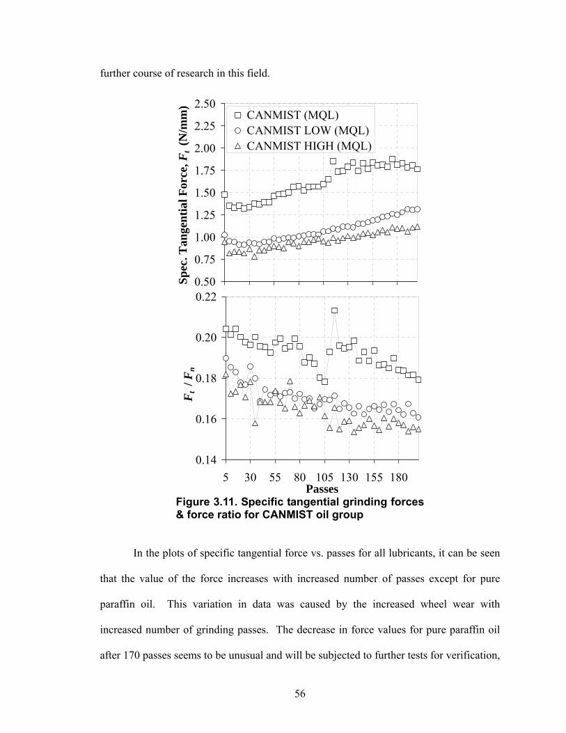
56

further course of research in this field.

0.50

0.75

1.00

1.25

1.50

1.75

2.00

2.25

2.50

Spec

. Tan

gent

ial F

orce

, Ft (

N/m

m)

CANMIST (MQL)CANMIST LOW (MQL)CANMIST HIGH (MQL)

0.14

0.16

0.18

0.20

0.22

5 30 55 80 105 130 155 180Passes

Ft /

Fn

Figure 3.11. Specific tangential grinding forces & force ratio for CANMIST oil group

In the plots of specific tangential force vs. passes for all lubricants, it can be seen

that the value of the force increases with increased number of passes except for pure

paraffin oil. This variation in data was caused by the increased wheel wear with

increased number of grinding passes. The decrease in force values for pure paraffin oil

after 170 passes seems to be unusual and will be subjected to further tests for verification,

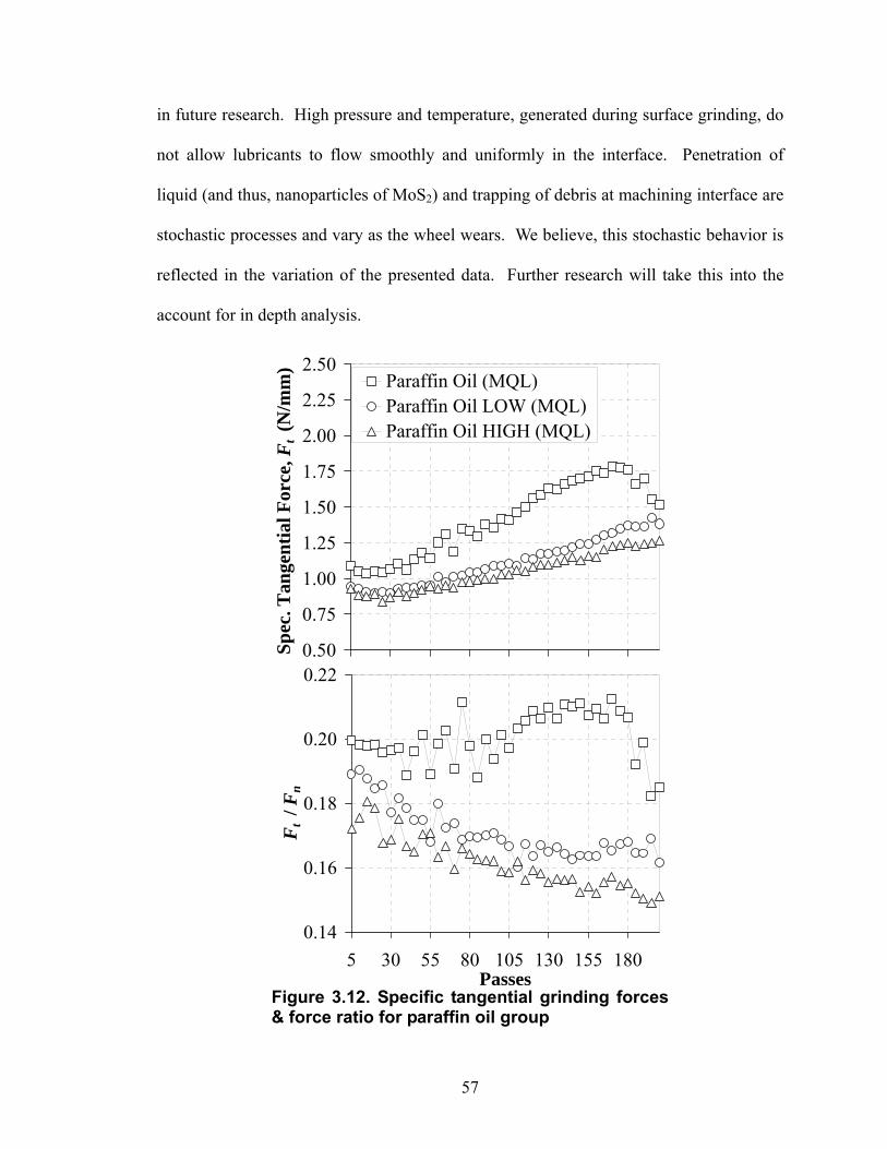
57

in future research. High pressure and temperature, generated during surface grinding, do

not allow lubricants to flow smoothly and uniformly in the interface. Penetration of

liquid (and thus, nanoparticles of MoS2) and trapping of debris at machining interface are

stochastic processes and vary as the wheel wears. We believe, this stochastic behavior is

reflected in the variation of the presented data. Further research will take this into the

account for in depth analysis.

0.50

0.75

1.00

1.25

1.50

1.75

2.00

2.25

2.50

Spec

. Tan

gent

ial F

orce

, Ft (

N/m

m)

Paraffin Oil (MQL)Paraffin Oil LOW (MQL)Paraffin Oil HIGH (MQL)

0.14

0.16

0.18

0.20

0.22

5 30 55 80 105 130 155 180Passes

Ft /

Fn

Figure 3.12. Specific tangential grinding forces & force ratio for paraffin oil group

58

It should also be noted that the number of grinding passes throughout the

experiment was quite large (200 passes). Under such conditions, tangential grinding

force and force ratio values of MQL grinding with nMoS2 based lubricants seems to be

far better than those of base fluids and flood lubrication.

0.75

0.90

1.05

1.20

1.35

1.50

1.65Sp

ec. T

ange

ntia

l For

ce, F

t (N

/mm

)

Soybean Oil (MQL)Soybean Oil LOW (MQL)Soybean Oil HIGH (MQL)

0.14

0.15

0.16

0.17

0.18

0.19

5 30 55 80 105 130 155 180Passes

Ft /

Fn

Figure 3.13. Specific tangential grinding forces & force ratio for soybean oil group

59

The above observed characteristic behaviors of nMoS2 based lubricants, namely,

enhanced penetration and entrapment at grinding interface, formation of tribofilm, base

fluid chemistry and effects of concentration of MoS2 nanoparticles on MQL grinding

performance will be analyzed in depth in future research.

3.3.4. G-ratio

Wheel life in grinding process is expressed in terms of grinding ratio or G-ratio

and is defined as the volume of material removed per unit volume of grinding wheel wear.

Wheels with a high G-ratio last longer than those with lower G-ratios (Krueger et al.,

2000). The grinding wheel wear occurs due to the friction between the abrasive grains

and the workpiece. High fluid lubricating capacity reduces the wear on the grinding

wheel by decreasing grain-workpiece friction, allowing the abrasive grains to remain

bound to the binder for longer periods and leading to lower wear of the tool (Silva et al.,

2005).

The G-ratio results for all the grinding experiments are shown in Figure 3.14. All

the MQL grinding operations with pure oil based fluids have much higher G-ratio

(ranging from 28 to 42) than flood cooling with water-based Cimtech 500 synthetic

grinding fluid. This can be attributed to the excellent lubricating capacity of oil based

fluids and to the good lubricating conditions provided by MQL, which give much lower

grinding forces as discussed in previous section.

It is important to note that G-ratio is higher for high concentration of nMoS2

additive conditions for all the base oils, including soybean oil. We believe that this can

be explained by the reduction in grinding forces with nMoS2 additives, thereby, ensuring

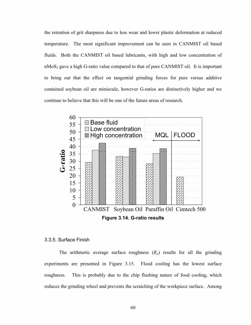
60

the retention of grit sharpness due to less wear and lower plastic deformation at reduced

temperature. The most significant improvement can be seen in CANMIST oil based

fluids. Both the CANMIST oil based lubricants, with high and low concentration of

nMoS2 gave a high G-ratio value compared to that of pure CANMIST oil. It is important

to bring out that the effect on tangential grinding forces for pure versus additive

contained soybean oil are miniscule, however G-ratios are distinctively higher and we

continue to believe that this will be one of the future areas of research.

05

1015202530354045505560

G-r

atio

Base fluidLow concentrationHigh concentration

CANMIST Soybean Oil Paraffin Oil Cimtech 500

MQL FLOOD

Figure 3.14. G-ratio results

3.3.5. Surface Finish

The arithmetic average surface roughness (Ra) results for all the grinding

experiments are presented in Figure 3.15. Flood cooling has the lowest surface

roughness. This is probably due to the chip flushing nature of food cooling, which

reduces the grinding wheel and prevents the scratching of the workpiece surface. Among

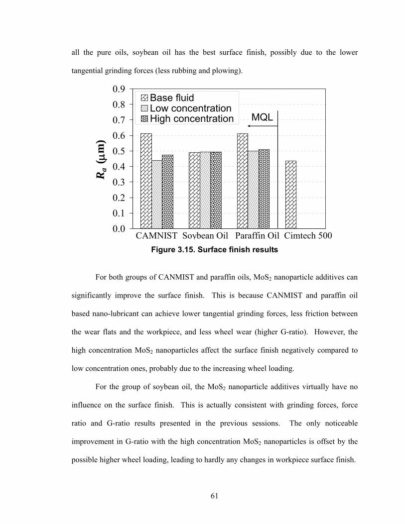
61

all the pure oils, soybean oil has the best surface finish, possibly due to the lower

tangential grinding forces (less rubbing and plowing).

0.00.10.20.30.40.50.60.70.80.9

Ra

( μm

)Base fluidLow concentrationHigh concentration

CAMNIST Soybean Oil Paraffin Oil Cimtech 500

MQL

Figure 3.15. Surface finish results

For both groups of CANMIST and paraffin oils, MoS2 nanoparticle additives can

significantly improve the surface finish. This is because CANMIST and paraffin oil

based nano-lubricant can achieve lower tangential grinding forces, less friction between

the wear flats and the workpiece, and less wheel wear (higher G-ratio). However, the

high concentration MoS2 nanoparticles affect the surface finish negatively compared to

low concentration ones, probably due to the increasing wheel loading.

For the group of soybean oil, the MoS2 nanoparticle additives virtually have no

influence on the surface finish. This is actually consistent with grinding forces, force

ratio and G-ratio results presented in the previous sessions. The only noticeable

improvement in G-ratio with the high concentration MoS2 nanoparticles is offset by the

possible higher wheel loading, leading to hardly any changes in workpiece surface finish.

62

3.3.6. Summary

It is shown for the first time that nanoparticles of MoS2 could provide key value

addition in MQL grinding, when using various off the shelf base fluids such as paraffin

oil, soybean oil and CANMIST oil. Also, it is reported that the nanoparticles of MoS2

offer unique advantages in MQL when they present the possibility of navigating in the

grinding zone and delivering reduction of grinding forces (27% for CANMIST oil group,

21% for paraffin oil based group and 9% for soybean oil group), and most distinctively

increase life of expensive grinding wheels by increasing G-ratio (46% for CANMIST oil

group, 35% in paraffin oil group and 15% in soybean oil group). Superior grinding

performance with minimum application of MoS2 based lubricants (5 ml/min compared to

5400 ml/min application in flood cooling) shows its cost-effectiveness. In addition,

MoS2 nanoparticle additives can improve the surface roughness (except for soybean oil

group). However, compared to flood cooling, MQL still has problems of inefficient ship

flushing, resulting in poorer surface finish.

Overall, this research presents a significant opportunity for fundamental science

and sustainable engineering solution for MQL grinding and needs further investigation.

3.4. Micro-scale Mechanism of MQL Grinding using Nanofluids

Material removal during grinding occurs as abrasive grains interact with the

workpiece material. Malkin (1989) proposed a grinding force model, reasoning that the

grinding forces can be considered to consist of cutting and sliding components. The

cutting component has two mechanism involved: (1) chip-formation, which is the actual

material removal process, and (2) plowing, which is the deformation of workpiece

63

material without removal. It can be considered as the side flow of material from the

cutting path to the ridges (plastic deformation). The sliding component is contributed to

the dulled flattened tips on the abrasive grains sliding against the workpiece surface

without removing any material.

Good lubrication in the grinding zone can largely reduce the sliding forces. The

lubricating properties of solid lubricant such as MoS2 are attributed to a layered structure

on the molecular level with weak bonding between layers. Such layers are able to slide

relative to each other with minimal applied force, thus resulting in low friction properties.

In MQL grinding using oil based nanofluids, it is believed that the suspended MoS2

nanoparticle additives can navigate at the machining interface to yield and scarify for

delivering a tribofilm to provide selective lubrication at tool-workpiece interface and the

transient (explosive) evaporation of oil molecules overcoated on the nanoparticles acting

as an effective vehicle for heat transfer, and as a result significantly reduce frication.


In this chapter, MQL grinding (conventional abrasive wheels) of cast iron using

water based and oil based nanofluids was investigated. Grinding performance is

evaluated and compared in terms of grinding force, G-ratio, and surface roughness, etc.

Water-based Al2O3 and diamond nanofluids were applied in MQL grinding

process and the grinding results were compared with those of pure water. Dispersion of

solid particles was found to play an important role, especially when a slurry layer was

formed. The slurry layer generated higher G-ratio (less wheel wear), smaller grinding

forces and better surface finish. Experimental results showed that G-ratio, defined as the

64

volume of material removed per. unit volume of grinding wheel wear, could be improved

with high concentration nanofluids. MQL grinding showed that it could significantly

reduce the grinding temperature compared to dry grinding. However, there is no

significant difference in grinding temperature when using nanofluids. It was further

concluded that nanofluids are not able to provide superior cooling capacity in MQL

grinding process. Thus, it was suggested that the future research of MQL grinding using

nanofluids should focus on the advanced lubrication properties instead.

The tribological behavior and performance of oil based cutting fluids with novel

molybdenum disulphide (MoS2) nanoparticle additives in MQL grinding were also

studied. It is shown for the first time that MoS2 nanoparticle additives can offer unique

advantages in MQL, that is, reducing grinding forces, increasing G-ratio, and improving

the surface finish (compared to that of base fluids except for soybean oil group).

However, compared to flood cooling, MQL still has problems of inefficient ship flushing,

resulting in poorer surface finish. The experimental results further imply that it is

possible to improve the tribological properties of the cutting fluids by adding lubricating

nanoparticles, and consequently to enhance the performance of MQL grinding.

65

CHAPTER 4

GRINDING TEMPERATURE MEASUREMENT AND ENERGY

PARTITION

A new thermocouple fixating method for grinding temperature measurement is

presented. Unlike the conventional method using a welded thermocouple, this new

method uses epoxy for affixing the embedded thermocouple within a blind hole in the

workpiece subsurface. During grinding, the thermocouple junction is exposed and

bonded to provide direct contact with the ground surface by the smearing of workpiece

material. Experiments were conducted to evaluate this simplified thermocouple fixating

method including the effect of thermocouple junction size. Heat transfer models were

applied to calculate the energy partition for grinding under dry, wet, and MQL conditions.

For shallow-cut grinding of cast iron using a vitreous bond aluminum oxide wheel,

the energy partition, ratio of the energy entering the workpiece, using a small wheel depth

of cut of 10 μm was estimated as 84% for dry grinding, 84% for MQL grinding, but only

24% for wet grinding. Such a small energy partition with wet grinding can be attributed

to cooling by the fluid at the grinding zone. Increasing the wheel depth of cut to 25 μm

for wet grinding resulted in a much bigger energy partition of 92%, which can

66

be attributed to fluid film boiling and loss of cooling at the grinding zone.

When using vitrified bond CBN wheel, the energy partition was estimated as 68%

for dry grinding, 54% for MQL grinding, and 13% for wet grinding. Experimental results

showed that the insufficient cooling problem of MQL grinding is not as significant using

the vitrified CBN wheel, which makes the MQL grinding feasible in the high volume

production.

4.1. Introduction

As mentioned in Chapter 1, the grinding process generates a very high input of

energy per unit volume of work-material removed. Virtually all the energy is converted

to heat, which can cause high workpiece temperature and related thermal damage such as

grinding burn, phase transformation, tensile residual stresses, surface cracks, reduced

fatigue strength, thermal distortion and inaccuracies (Malkin, 1989). Therefore, heat

transfer in grinding is of significant importance.

Experimental investigations of heat transfer in grinding require accurate

temperature measurements. Methods for temperature measurement in grinding include

thermal imaging (Sakagami et al., 1990; Hwang et al., 2004), optical fiber (Ueda, 1986;

Ueda and Sugita, 1992; Curry et al., 2003), foil/workpiece (single pole) thermocouple

(Rowe et al., 1996; Xu et al., 2003; Huang and Xu, 2004; Batako et al., 2005; Lefebvre et

al., 2006), and embedded (double pole) thermocouple (Littman and Wulff, 1995; Kohli et

al., 1995; Guo et al., 1999; Xu and Malkin, 2001; Upadhyaya and Malkin, 2004; Kim et

al., 2006). The embedded thermocouple method is the most widely used of these

techniques because of its relative simplicity, low cost, accuracy, and reliability. With this

67

method, a double pole thermocouple is welded to the bottom of a blind hole drilled close

to the ground surface from the underside of the workpiece (Guo et al., 1999; Upadhyaya

and Malkin, 2004). Welding the small tip of a double pole thermocouple at the bottom of

the small hole requires special discharge welding equipment and skills. During grinding,

the thermocouple measures the temperature below the workpiece surface during

successive passes until the welded junction is broken by the grinding action. Accurately

determining the position of the temperature measurement below the surface being ground

is complicated by its size and also the blind hole. Furthermore the embedded

thermocouple and the hole can disturb the local temperature field. Therefore it is

desirable to make the thermocouple and hole very small.

The present investigation was undertaken to evaluate a simpler embedded

thermocouple method for grinding temperature measurement which uses epoxy instead of

welding to affix the thermocouple at the bottom of the blind hole. During grinding the

thermocouple junction is exposed and bonded to the workpiece by smearing of the

workpiece material, thereby providing direct contact with the workpiece surface and a

direct temperature measurement at the workpiece surface. The proposed grinding

temperature measurement method was then used to study the energy partition for dry, wet

(flood cooling), and MQL grinding.

On the other hand, to reduce the energy partition to the workpiece, and overcome

the problem of insufficient workpiece cooling, CBN wheels are considered for MQL

grinding. CBN grains have very high thermal conductivity, which enhances heat

conduction away from the grinding zone to the wheel (Lavine et al., 1989; Upadhyaya

and Malkin, 2004). For conventional shallow-cut grinding of steels with Al2O3 wheels,

68

energy partition has been typically found to range from 60% to 85% (Malkin, 1989;

Kohli et al., 1995). While significantly lower energy partition values of about 20% were

found for grinding with a resin bond CBN wheel (Kohli et al., 1995). Furthermore, with

a porous vitrified CBN wheel, much lower energy partition values of only 3% to 8% were

reported by Guo et al. (1999) and Varghese et al. (2000). This additional reduction in the

energy partition, beyond what was obtained with the resin bond CBN wheel, was

attributed to cooling at the grinding zone by fluid entrapped in the wheel pores

(Upadhyaya and Malkin, 2004). Although CBN wheels are widely used in industrial

production, there is limited research in CBN MQL grinding (Silva et al., 2005).

In the first part of this chapter, the new thermocouple fixating method for grinding

temperature measurement was first investigated. The experiments were conducted which

compare the performance of epoxy fixated thermocouples with that of welded

thermocouples. In the second part, MQL grinding performance of the vitrified CBN

wheel using soybean oil, and soybean carbon nanotube (CNT) additives was studied.

The experimental results including grinding forces, surface finish, grinding temperature

and especially the energy partition are presented.

4.2. Thermocouple Fixating Method for Grinding Temperature Measurement

4.2.1. Grinding Test Setup

Straight surface plunge grinding experiments (no crossfeed) were conducted on an

instrumented Chevalier Model Smart-B818 surface grinding machine using the setup

shown in Figure 4.1. The grinding wheel was vitreous bonded aluminum oxide (Saint-

Gobain/Norton 32A46-HVBEP) of initial diameter ds=177.8 mm and width bs=12.7 mm.

69

The workpiece material was Dura-Bar 100-70-02 ductile iron with a carbon content of

3.5-3.9%, hardness 50 Rockwell C, thermal conductivity 63 W/m·K, and thermal

diffusivity 1.63×10-7 m2/s. The workpieces were of length 58 mm in the grinding

direction and width bw=6.5 mm corresponding to the grinding width. Experiments were

conducted without fluid (dry), under wet (flood) application conditions, and with

Minimum Quantity Lubrication (MQL). The same fluid (5 vol% Cimtech 500 synthetic

grinding fluid in water) was used both for MQL and flood application. MQL application

utilized a special fluid deliver system provided by AMCOL, as mentioned in Chapter 3.

The flow rate was 5400 ml/min for flood (wet) grinding, but only 5 ml/min for MQL.

All experiments were conducted in the down mode with the wheel and workpiece

velocities in the same direction at the grinding zone (Figure 4.1). The wheel velocity was

vs=30 m/s. Two sets of grinding parameters were used: fine grinding with a workpiece

velocity of vw=2.4 m/min and depth of cut a=10 μm, and more aggressive grinding with

vw=3.0 m/min and a=25 μm. Prior to each grinding experiment, the wheel was dressed

by taking a minimum of 15 passes across the rotating wheel using a rotary diamond disk

dresser with a diameter of 96 mm and width of 3.8 mm (provided by Saint-Gobain) in the

up mode with a speed ratio (ratio of peripheral dresser velocity to wheel velocity) of −0.4,

a radial depth of 10 μm, and a traverse velocity of 500 mm/min. During grinding, the

normal and tangential grinding force components were measured using a Kistler Model

9257A piezoelectric dynamometer, and the temperature was measured using an epoxied

or welded thermocouple, as shown in Figure 4.1(b). Both grinding force and temperature

data were collected simultaneously at a 5 kHz sampling rate. The workpiece was allowed

to cool down completely after each grinding pass.

70

(a)

(b)

Figure 4.1. Experimental setup: (a) overview of the setup and (b) schematic drawing of grinding temperature measurement

4.2.2. Thermocouple Fixating

Most experiments were conducted with expoxied thermocouples which were

affixed to the bottom of a blind hole using a high temperature epoxy (Permabond 920).

Both 30 and 46 gage type K thermocouples were used to investigate the effect of junction

Workpiece

Nozzle

71

size. The junction diameter was 0.60−0.80 mm for the 30 gage thermocouple and

0.20−0.25 mm for the 46 gage thermocouple. A blind hole was drilled from the

underside of the workpiece to within 1−2 mm of the workpiece surface by electrical

discharge machining (EDM) with a tubular electrode. The hole diameter was 0.8 mm for

the 30 gage thermocouples and 0.3 mm for the 46 gage thermocouples. The tubular EDM

electrode left a knob at the bottom of the blind hole, as shown in the cross-sectional view

in Figure 4.2(a), which made it difficult to affix the thermocouple. Therefore EDM with

a solid electrode of smaller diameter was subsequently used to remove the knob and

create a tapered concave pocket as shown in Figure 4.2(b). Figure 4.3(a) shows a cross-

section of the 30 gage thermocouple junction inside a 0.8 mm diameter hole.

(a) (b) Figure 4.2. Cross-section view of blind hole tips: (a) EDM drilled using a tubular electrode and (b) EDM modified using a solid electrode

During grinding, the thermocouple junction is exposed (Figure 4.3(b)) and the

deformed workpiece connects the thermocouple junction to the workpiece (Figure 4.4(a))

0.25 mm 0.25 mm

72

for temperature measurement. The thermocouple was grounded in order to reduce noise

and avoid the electric charge produced by the mechanical contact. The time constant of

the embedded thermocouple was on the order of 1 ms (Xu and Malkin, 2001). Whether

this response time is sufficiently fast may be ascertained by comparing to the

characteristic time it takes for a point on the workpiece surface to pass through the

grinding zone, which can be obtained as the contact length lc ( ads= ) divided by the

workpiece velocity vw (Xu and Malkin, 2001). In this study, the characteristic time was

estimated as 33 ms, which is more than an order of magnitude bigger than the time

constant of the embedded thermocouple.

(a) (b)

Figure 4.3. Illustration of thermocouple fixating: (a) cross-section view and (b) schematic drawing

The sizes of the hole and thermocouple junction need to be closely matched. If

the hole is too large, a good connection between the thermocouple junction and

workpiece is not obtained, as seen in Figure 4.4(b). It will be seen that this can adversely

affect the temperature measurement.

1 mm

73

(a) (b) Figure 4.4. Illustration of thermocouple fixating: (a) closely matched thermocouple tip and hole with good connection and (b) large hole leading to a gap surrounding the thermocouple tip

A calibration test was conducted to verify that the epoxied thermocouple still

works even after part of the junction has been ground away. For this purpose, the ground

thermocouple and workpiece assembly shown in Figure 4.4 was submerged in ice-water

and in boiling water. Accurate temperature measurements were obtained.

For comparison, experiments were also conducted using welded thermocouples

(Figure 4.5). Welded thermocouples require a larger junction and a bigger hole than

epoxied thermocouples, which is a definite disadvantage. Furthermore, a welded

thermocouple usually breaks just as it begins to become exposed during grinding, so the

maximum temperature is actually measured slightly below the ground surface.

Accurately determining the temperature at the workpiece surface with a welded

thermocouple is usually done by extrapolation of subsurface temperature measurements

to the surface (Guo and Malkin, 1996a). By contrast, an epoxied thermocouple maintains

direct contact with the workpiece surface as the junction is ground, thereby providing a

direct measurement of the surface temperature (Figure 4.4(a)).

Exposed thermocouple

Workpiece

Gap 1.0 mm

Workpiece

Connection

0.3 mm

Exposed thermocouple (46 gage)

Workpiece

Exposed thermocouple (30 gage)

Connection0.8 mm

74

(a) (b) Figure 4.5. Difference between (a) welded thermocouple and (b) epoxied thermocouple

4.2.3. Experimental Design

Grinding conditions for all experiments are listed in Table 4.1. Experiments with

welded thermocouples are designated as Exp. W. From eight sets of experiments with

epoxied thermocouples, four marked as Exps. E1, E2, ES1, and ES2, were conducted for

the same grinding conditions as with the welded thermocouples. For ascertaining the

effect of junction size, smaller 46 gage thermocouples were used in Exps. ES1 and ES2.

All the other experiments were conducted using 30 gage thermocouples. One test, Exp.

E3, was conducted with an epoxied thermocouple placed in an oversized hole, as seen in

Figure 4.4(b), to identify the effect of hole diameter on the temperature measurement.

Experiments EW1 and EW2 refer to wet grinding using different parameters.

Experiment EM was with MQL.

75

Table 4.1. Experimental matrix design Experiment designation W E1 E2 E3 ES1 ES2 EM EW1 EW2Fixturing method Welded Epoxied Thermocouple wire gage 30 30 30 30 46 46 30 30 30 Depth of cut (μm) 10 25 Workpiece velocity (m/min) 2.4 3

Grinding fluid flow rate (ml/min) N/A (dry) 5 5400

4.2.4. Temperature Rise

During grinding, both the welded and epoxied thermocouples measure the

temperatures at a distance z below the workpiece surface (Figure 4.3(b)). Temperature

measurements with the epoxied thermocouple in Figure 4.6 show the peak temperature

rise for each subsequent grinding pass progressively increasing until the thermocouple is

fully exposed (Figure 4.4(a)) and the connection between the thermocouple junction and

workpiece is established. At this point the peak temperature rise is reached, and it

remains nearly constant for a number of additional grinding passes. The location of the

reference surface at z=0 can be defined by where this steady-state period begins, as

illustrated in Figure 4.6. The steady-state period in Figure 4.6 persists for more passes

with the bigger 30 gage thermocouple than with the smaller 46 gage thermocouple.

76

100

200

300

400

500

600

0 10 20 30 40 50Grinding passes

Peak

tem

pera

ture

rise

(°C

)

0 10 20 30 40 50Grinding passes

46 gage thermocouple (Exp. ES1)

Define position z=0

Steady workpiece surface temperature measurements

30 gage thermocouple (Exp. E1)

Define position z=0

Steady workpiece surface temperature measurements

Figure 4.6. Peak temperature rise vs. grinding passes for epoxied thermocouple method

For a welded thermocouple, the reference of z=0 is usually defined at the position

where the thermocouple begins to be exposed and the maximum peak temperature rise is

measured. However, this peak temperature probably occurs slightly below the surface

since the next grinding pass usually damages the welded connection between the

thermocouple and the workpiece.

Measured temperature rises for dry grinding conditions are presented in Figure

4.7. For all experiments, the peak temperature is bigger closer to the surface at smaller

depth z. Note that when the thermocouple is further down below the ground surface

(z≥0.2 mm), the temperature measured using the welded thermocouple (Exp. W)

decreases faster than the temperature measured using the epoxied thermocouple, which

suggests poor thermal contact. When grinding at the surface where z=0, good contact is

obtained between the workpiece surface and epoxied thermocouple (see Figure 4.4(a)).

77

This can explain why the maximum temperature measured using an epoxied

thermocouple is higher than for the welded thermocouple under the same grinding

conditions, except for Exp. E3 (small thermocouple in large hole) where a gap exists

between the thermocouple junction and the workpiece (Figure 4.4(b)). The lower

temperature measured with the welded thermocouple is a further indication that its

maximum peak temperature is measured below the surface just as the junction begins to

be exposed. The data obtained with the smaller 46 gage thermocouples in Exps. ES1 and

ES2 generally show a faster response as well as a faster cooling rate than with the bigger

30 gage thermocouples in Exps. E1, E2 and E3. This can be attributed to reduced size

and lower thermal inertia.

78

0

100

200

300

400

500

600

Tem

pera

ture

rise

(o C) z = 0

z = 0.1

z = 0.2

z = 0.3

Depth (mm)Exp. W Exp. E1

0

100

200

300

400

500

600

Tem

pera

ture

rise

(o C) z = 0

z = 0.1

z = 0.2

z = 0.3

Depth (mm)Exp. E2 Exp. E3

0

100

200

300

400

500

600

0 0.2 0.4 0.6 0.8Time (s)

Tem

pera

ture

rise

(o C) z = 0

z = 0.05z = 0.10z = 0.15z = 0.20

Depth (mm)Exp. ES1

0 0.2 0.4 0.6 0.8Time (s)

Exp. ES2

Figure 4.7. Temperature rise at different depth in dry grinding: Exp. W with welded thermocouple (30 gage), Exps. E1, E2, and E3 with epoxied thermocouple (30 gage), and Exps. ES1 and ES2 with epoxied thermocouple (46 gage)

79

A comparison of grinding temperatures measured at the surface (z=0) under dry

conditions is presented in Figure 4.8. The peak temperature rises for Exps. E1 and E2 are

almost identical at 500°C. The peak temperature rises for Exps. ES1 and ES2 (smaller 46

gage thermocouples) are slightly higher, 525°C and 511°C, respectively, which can again

be attributed to the smaller junction size. The welded thermocouple (Exp. W) gives a

lower peak temperature rise (469°C), apparently because of its larger size and also

damage to the weld joint, as described above. Also the welded thermocouple requires a

larger hole diameter (1.5 mm) for electrical insulation, which could also lower the

measured temperature. For Exp. E3 with the bigger hole, the thermal connection is not

formed (Figure 4.4(b)) and the measured peak temperature is much lower (405°C).

0

100

200

300

400

500

600

0 0.2 0.4 0.6 0.8Time (s)

Tem

pera

ture

rise

(o C)

Exp. E1Exp. E2Exp. E3Exp. W

0 0.2 0.4 0.6 0.8Time (s)

Exp. E1

Exp. E2

Exp. ES1

Exp. ES2

Depth, z = 0Depth, z = 0

Figure 4.8. Measured grinding temperature at the workpiece surface at depth z=0 (dry condition)

80

0

30

60

90

120

0 0.2 0.4 0.6 0.8

Time (s)

Tem

pera

ture

rise

(o C) z = 0.3

z = 0.2z = 0.1z = 0

Depth (mm)Exp. EW1

(a)

0

100

200

300

400

500

0 0.2 0.4 0.6 0.8

Time (s)

Tem

pera

ture

rise

(o C)

z = 0.3z = 0.2z = 0.1z = 0

Depth (mm)Exp. EW2

(b)

Figure 4.9. Temperature rise in wet grinding, different grinding conditions: (a) depth of cut, a=10 μm and workpiece velocity, vw=2.4 m/min, and (b) a=25 μm and vw=3 m/min

81

Experiment EW1 was conducted under wet conditions with the same grinding

parameters as in dry grinding, but the maximum temperature rise of 106°C (Figure

4.9(a)) was much lower. This temperature rise is comparable to or slightly less than the

film boiling temperature of the water-based grinding fluid. In the absence of film boiling,

the grinding fluid should provide significant cooling at the grinding zone, which is

usually much more likely with creep feed grinding than with conventional shallow cut

grinding (Fuh and Huang, 1994). In another wet grinding test Exp. EW2 under more

aggressive conditions (vw=3 m/min and a=25 μm), the peak temperature rise (474°C)

greatly exceeded the film boiling temperature of the grinding fluid.

0

100

200

300

400

500

0 0.2 0.4 0.6 0.8

Time (s)

Tem

pera

ture

rise

(o C)

z = 0.3z = 0.2z = 0.1z = 0

Depth (mm)Exp. EM

Figure 4.10. Temperature rise at different depths in MQL grinding (grinding fluid flowrate = 5 ml/min)

The temperature rise for Exp. EM with MQL is shown in Figure 4.10. The peak

temperature rise of 444°C is about 60°C lower than for dry grinding (see Figure 4.8).

82

This lower temperature can be attributed, at least in part, to lubrication by MQL, which

reduced the average tangential grinding force per unit width, Ft/bw, from about 2.0 N/mm

with dry grinding to 1.8 N/mm with MQL.

4.2.5. Energy Partition

4.2.5.1. Traditional heat transfer models

Straight surface grinding experiments were conducted as shown in Figure 4.11

where a wheel of diameter ds rotating with a peripheral velocity vs removes a depth a of

material from the workpiece as it passes under the wheel at velocity vw. Virtually all the

grinding energy expended at the grinding zone is converted to heat, which is transported

to the workpiece, grinding wheel, chips and grinding fluid. The geometrical grinding

zone is the region of length lc (= ads ) where the wheel interacts with the workpiece.

vw

vs

Workpiece

a

ds

Grinding wheel

xaxb

2l

Heat flux q(x)Nozzle

Grinding fluid

Figure 4.11. Schematic drawing of heat transfer in down grinding

83

The temperatures generated at the grinding zone can be calculated by considering

the grinding zone as a band source of heat of length lc which moves along the surface of

the workpiece at the workpiece velocity vw. A critical parameter for this thermal analysis

is the energy partition ε, which is defined as the fraction of the grinding energy

transported as heat to the workpiece at the grinding zone. Since the maximum grinding

zone temperature rise θmax is measured and the total energy input can be readily

calculated from the tangential force measurement, the thermal analysis can be used to

evaluate the energy partition which occurred for grinding using the relationships (Guo

and Malkin, 1992):

max4/1s

4/12/1w

2/1ww

davk

q θβα

= (4.1)

cw

st

lbvF/q=ε (4.2)

where q is the heat flux into the workpiece, kw the workpiece thermal conductivity, αw the

thermal diffusivity of workpiece, Ft the tangential grinding force, bw the width of the

workpiece, and β a constant which depends on the heat source shape. In this study,

β=1.06 for the triangular shape heat source (Guo and Malkin, 1992).

Guo and Malkin (1996a; 1996b) developed an inverse heat transfer model based

on the moving heat source theory (Jaeger, 1942). For a semi-infinite body, the quasi-

steady state temperature distribution θw(x,z) in the workpiece within a region [xa, xb] is

given by

84

( ) ( ) ( ) ξξξθ dzxqzx a

b

x

x ww ,,, Φ= ∫ (4.3)

where qw(ξ) is the heat flux into workpiece, ξ a local coordinate in the x-direction, Φ a

function defined as:

( ) ( ) ( )[ ]⎭⎬⎫

+−⎩⎨⎧= −− 2122

02

21 /w/xv

w

zxv

Kek

,z,x ww ξαπ

ξΦ αξ (4.4)

where K0 is the modified Bessel function of the 2nd kind of order zero. If the region [xa,

xb] is divided into n very small sections [ξi, ξi+1] of equal length, where

( )

in

xxx

in

xxx

babi

babi

−+=

−−

+=

+1

1

ξ

ξ (4.5)

The heat flux qw(ξi) within each section can be approximated as a constant qi.

Equation (4.3) can be rewritten as:

( ) ( )∫∑ + Φ==

1 ,,,1

i

i

dzxqzxn

iiw

ξ

ξξξθ (4.6)

At a depth z beneath the workpiece surface, discrete temperatures Tj were

measured at n equally spaced points xj (j=1,2,…,n) as the workpiece moves at speed vw

and the data was collected at fixed frequency. These xj may or may not coincide with

local coordinate ξi at the surface. Consequently, we have the following n equations:

( ) ( ) njdzxqzx i

ij

n

iijw ,...,2,1 ,,, 1

1=Φ= ∫∑ +

=

ξ

ξξξθ (4.7)

85

Substituting the n measured temperature Tj for θw(xj,z) into Equation (4.7) leads to

a system of n simultaneous equations:

j

n

iiji Tqc =∑

=1 (4.8)

where cji are coefficients defined as:

( ) njidzxc i

ijji ,...,2,1, ,,1 =Φ= ∫

+ξ

ξξξ (4.9)

Equation (4.8) can also be written in the matrix form:

⎥⎥⎥⎥⎥⎥

⎦

⎤

⎢⎢⎢⎢⎢⎢

⎣

⎡

⋅=

⎥⎥⎥⎥⎥⎥

⎦

⎤

⎢⎢⎢⎢⎢⎢

⎣

⎡

⋅⎥⎥⎥⎥⎥⎥

⎦

⎤

⎢⎢⎢⎢⎢⎢

⎣

⎡

⋅⋅⋅⋅⋅⋅⋅⋅⋅⋅⋅⋅

⋅

nnnnn

n

T

TTT

q

qqq

cc

cccccc

cccc

3

2

1

3

2

1

1

333231

232221

1131211

(4.10)

For a given grinding condition, coefficients cji can be numerically evaluated and

thus the heat flux can be determined if the temperature profile at a particular depth z is

measured. Given the heat flux distribution, the energy partition, which is the fraction of

the grinding energy transported as heat to the workpiece at the grinding zone, can be

found by integrating the heat flux over the entire grinding zone. Although it has the most

flexibility, this method has stability problem and is very sensitive to the input temperature

measurements.

On the other hand, with the assumption of heat flux shape (for example,

rectangular or triangular shape), the energy partition can also be found by matching the

experimentally measured temperatures with the predicted values (Equation (4.8)). This is

so called “temperature matching method”, and is more widely used (Kohli et al., 1995;

86

Guo and et al., 1999; Xu and Malkin, 2001; Upadhyaya and Malkin, 2004). In this study,

the temperature method is used for energy partition calculation.

4.2.5.2. Energy partition by curve fitting

Experimental measurements of peak temperature rise versus depth z are plotted in

Figure 4.12. In each case, the peak temperature rise increases closer to the surface. The

inverse heat transfer model can be used to predict grinding temperature profiles at

different depths. Therefore, the energy partition can be determined by matching the peak

temperatures at different depth for the measured temperatures and the theoretical results.

A Matlab program was developed for obtaining a least square fit. The energy partition

calculated using this method is designated as εfitting.

0

100

200

300

400

500

600

700

0.00 0.05 0.10 0.15 0.20 0.25 0.30Depth, z (mm)

Peak

tem

pera

ture

rise

(°C

)

Exp. W = 72% Exp. EW1 = 21%Exp. E1 = 81% Exp. EW2 = 90%Exp. E2 = 84% Exp. EM = 70%

Exp. ES1 Exp. ES2

ε fitting

ε fitting

ε fitting

ε fitting

ε fitting

ε fitting

R2=0.82

R2=0.85

R2=0.90

R2=0.73

R2=0.64

R2=0.81

Figure 4.12. Experimental and theoretical maximum temperature rise versus the depth z

87

For the welded thermocouple (Exp. W), it was found that εfitting=72% using the

least square fit over the entire range, as illustrated in Figure 4.12. However, the expoxied

thermocouple undermeasures the temperature when it is positioned far below the

workpiece surface, as discussed in the previous section. Consequently, not all the

experimental data points ranging from z=0 to z=0.3 mm are appropriate for curve fitting.

Therefore, the R2 value, which determines the goodness of fit, was used to select a cutoff

depth z0, i.e., data with depth z<z0, to maximize the R2 value. The best fit theoretical

curves and their corresponding R2 value for the epoxied thermocouple experiments are

plotted in Figure 4.12. The R2 value (=0.82) for the welded thermocouple is included for

comparison.

The data for the 30 gage epoxied thermocouples, except for Exp. EW1, match

well with theoretical curves only near the workpiece surface (cutoff depth z0≤0.15 mm).

Experiments E1, E2, and EM give εfitting=81%, εfitting=84%, and εfitting=70%, respectively.

However, the R2 value for Exp. EM (=0.64) is lower than for the other experiments.

Apparently the temperature measurements in Exp. EM have a larger variation than the

others due to discontinuous fluid delivery using the MQL device with 1−2 Hz pulsed

fluid delivery. For Exp. EW1, the temperature rise is below the fluid burn-out limit of

about 120°C. A theoretical curve with εfitting=21% matches the data fairly well over the

whole range (z0=0.3 mm) with R2=0.73. Such a low energy partition in this case indicates

effective cooling by the fluid at the grinding zone, as previously mentioned. For more

aggressive wet grinding, Exp. EW2, the temperature at the grinding zone was much

higher than the burnout limit, so cooling at the grinding zone should have been

ineffective. This can account for the much higher energy partition of εfitting ≈ 90%.

88

By contrast, the data obtained with the 46 gage epoxied thermocouple (Exps. ES1

and ES2), does not match any theoretical curves (R2<<1). In these cases, the measured

temperature is very low far below the ground surface. Apparently the small

thermocouple junction fits loosely in the blind hole leading to a much larger contact

thermal resistance. Nonetheless, when the connection between the thermocouple junction

and the workpiece starts to form during grinding (z<0.04 mm), the measured

temperatures increases substantially as seen in Figure 4.12.

4.2.5.3. Energy partition results by surface temperature matching

One important advantage with epoxied thermocouples is that temperature

measurements can be directly obtained at the workpiece surface as seen in Figure 4.6.

Therefore it should be possible to use these peak surface temperature measurements to

obtain more precise estimations of the energy partition values by matching the average of

these peak temperature rises with the theoretical values according to either the simple

heat transfer analysis (Equation (4.1)) or the inverse heat transfer model (Equation (4.8)).

Again for this purpose, a triangular heat source was assumed. For the welded

thermocouple, only the peak temperature rise at depth z=0 was used to calculate the

energy partition, since only one temperature measurement at the workpiece surface was

available.

The results are summarized in Table 4.2, which also includes corresponding

values for the specific tangential force, grinding power, and heat flux to the workpiece at

the grinding zone. The energy partitions obtained with both heat transfer models (εsimple

and εinverse) are almost identical, and they are also very close to the values obtained by

89

curve fitting (εfitting) with high R2 values (R2>0.8). When the R2 value is lower, the

estimated ε is less accurate. For Exp. EM, with R2=0.64, εfitting is about 14% lower than

the values obtained with both heat transfer models. Slightly higher energy partitions

were obtained with the epoxied thermocouples (Exps. E1 and E2) than with the welded

thermocouple (Exp. W) because the epoxied thermocouples indicate slightly higher

surface temperatures. Likewise higher energy partitions are also obtained with smaller

epoxied thermocouples (Exps. ES1 and ES2) than with larger ones (Exps. E1 and E2).

The very low energy partition of only 24% for the fine wet grinding test, Exp. EW1, can

be attributed mainly to effective cooling at the grinding zone below the film boiling

temperature, as previously indicated. With more aggressive wet grinding (Exp. EW2), the

grinding zone temperature greatly exceeded the fluid film boiling temperature, cooling at

the grinding zone became insignificant. The estimated energy partition of 84% for MQL

grinding, Exp. EM, is almost identical to the energy partition for dry grinding, so it can

be concluded that the minute amount of fluid applied by MQL provides virtually no

cooling at the grinding zone.

Table 4.2. Summary of heat transfer analysis in grinding experiments Exp. W E1 E2 ES1 ES2 EW1 EW2 EM Fixturing method Welded Epoxied Thermocouple wire gage 30 30 30 46 46 30 30 30 Max. temperature rise (°C) 469 493 503 525 511 106 474 444 Specific tangential force, Ft (N/mm) 2.00 2.05 2.09 1.96 2.00 1.50 2.40 1.79

Grinding power (W) 390 400 408 382 390 293 468 349 εsimple - simple model 78% 80% 80% 89% 85% 24% 92% 83%εinverse - inverse heat transfer 79% 82% 82% 90% 87% 24% 93% 84%εfitting - curve fitting 72% 81% 84% -- -- 21% 90% 70% - R2 for the curve fitting 0.82 0.89 0.90 -- -- 0.73 0.85 0.64 Heat flux into workpiece (W/mm2) 36.2 38.3 39.1 40.5 39.7 8.3 51.2 34.5

90

4.2.6. Summary

A new thermocouple fixating method was developed for grinding temperature

measurement which uses epoxy instead of spot welding to affix the tip of the

thermocouple to the bottom of a blind hole. Experiments were conducted to compare the

performance of epoxied and welded thermocouples. For expoxied thermocouples, the

good thermal contact was obtained as the thermocouple junction became exposed by

smearing of the workpiece material during grinding, thereby providing an accurate

measurement of the surface temperature at the grinding zone. For welded thermocouples,

the junctions tend to be damaged during grinding as they becomes exposed and the

maximum temperatures are slightly smaller than the temperatures measured with epoxied

thermocouples.

Grinding experiments and heat transfer analyses showed that grinding fluids

provide negligible cooling within the grinding zone as evidenced by the high energy

partitions which ranged from 84% to 92% for dry grinding, wet grinding, and MQL

grinding. An exception was observed for fine wet grinding which gave a much lower

energy partition of 24%, due to cooling within the grinding zone below the film boiling

temperature. Although cooling by the fluid may be ineffective within the grinding zone,

cooling can occur outside the grinding zone as evidenced by the much faster drop in the

measured temperature from its peak value with wet grinding (Figure 4.9) than with dry

grinding (Figure 4.8). Bulk cooling of the workpiece in this way can be an important

factor in controlling thermally induced dimensional inaccuracy and distortion. While

MQL is effective in providing lubrication, it can be seen by comparing the temperature

response curves for MQL (Figure 4.10) with those for dry grinding (Figure 4.9) that the

91

miniscule amount of applied fluid with MQL does not provide any significant cooling

outside the grinding zone. This is a major drawback which can limit the more

widespread application of MQL for grinding.

4.3. MQL Grinding using Vitrified CBN Wheels

From the previous section, it is confirmed that with convectional abrasive wheels

MQL does not provide significant cooling in grinding, resulting in a high energy partition

to the workpiece. To fundamentally lower the energy partition and reduce the workpiece

temperature (in order to avoid thermal damage), CBN grinding wheels are considered in

this section.

In addition, from Chapter 3, it is concluded that some nanoparticle additives may

improve the lubricating properties of the base fluids. However, although it is the best

lubricant among the three tested base oils, the soybean oil did not show any further

significant improvement with MoS2 nanoparticle additives. Therefore, soybean oil was

again chosen as for the MQL application in this study. In addition, another type of

nanoparticles - carbon nanotube (CNT) was mixed in soybean oil as the additive to

investigate the potential application of nano-lubricant in MQL grinding.

4.3.1. Experimental Procedure

Experiments of straight surface plunge grinding without crossfeed were

conducted on the same machine (Chevalier Model Smart-B818 surface grinding machine

with a 1.5 kW spindle). The experimental setup is shown in Figure 4.13(a), very similar

to the pervious setup. The vitreous bond CBN grinding wheel (Universal Abrasive

92

VB126-J160-VT2W19) was used. The grinding wheel is about 177.8 mm in diameter

and 12.7 mm in width. The surface speed of the wheel was 30 m/s. The work-material

was the same as before.

For wet grinding, the water-based Cimtech 500 synthetic grinding fluid at 5 vol%

was used. MQL grinding, shown in Figure 4.13(b), utilized the same fluid application

device provided by AMCOL (Hazel Park, Michigan). Soybean oil and soybean oil mixed

with CNT additives, denoted as CNT-soybean oil, were used for MQL application. The

CNT-soybean oil were prepared by mixing soybean oil with multi-wall carbon nanotubes

using 2 wt% lecithin as surfactant and subjected to 2 hrs of ultrasonic homogenization.

The added multi-wall carbon nanotubes (L-MWCNT-1020), provided by Shenzhen

Nanotech Port Co. in China, has outside diameter of 10-20 nm and length of 5-15 μm.

The flow rate was 5400 ml/min for flood (wet) grinding, but only 5 ml/min for MQL.

The grinding wheel was dressed at 2 μm down feed, 500 mm/min traverse speed and –0.4

speed ratio using a rotary diamond disk, which is 96 mm in diameter and 3.8 mm in

width.

93

(a)

(b)

(c) Figure 4.13. Experimental setup: (a) overview, (b) MQL fluid delivery device, and (c) illustration of grinding temperature measurement

Two sets of experiments were conducted. The first set of the experiments

investigates the influence of down feed and feed rate on grinding forces and surface

finish under dry, MQL, and flood cooling conditions. The down feeds and feed rates as

well as the corresponding specific material removal rate (MRR) in this set of experiments

are listed in Table 4.3. The specific MRR is defined as the material removal rate per unit

width. The normal and tangential grinding forces were measured using a Kistler Model

Air

Liquid hose

Fluid reservoir

Air hose

Air hose

Liquid hose

Workpiece

CBN Wheel

Nozzle

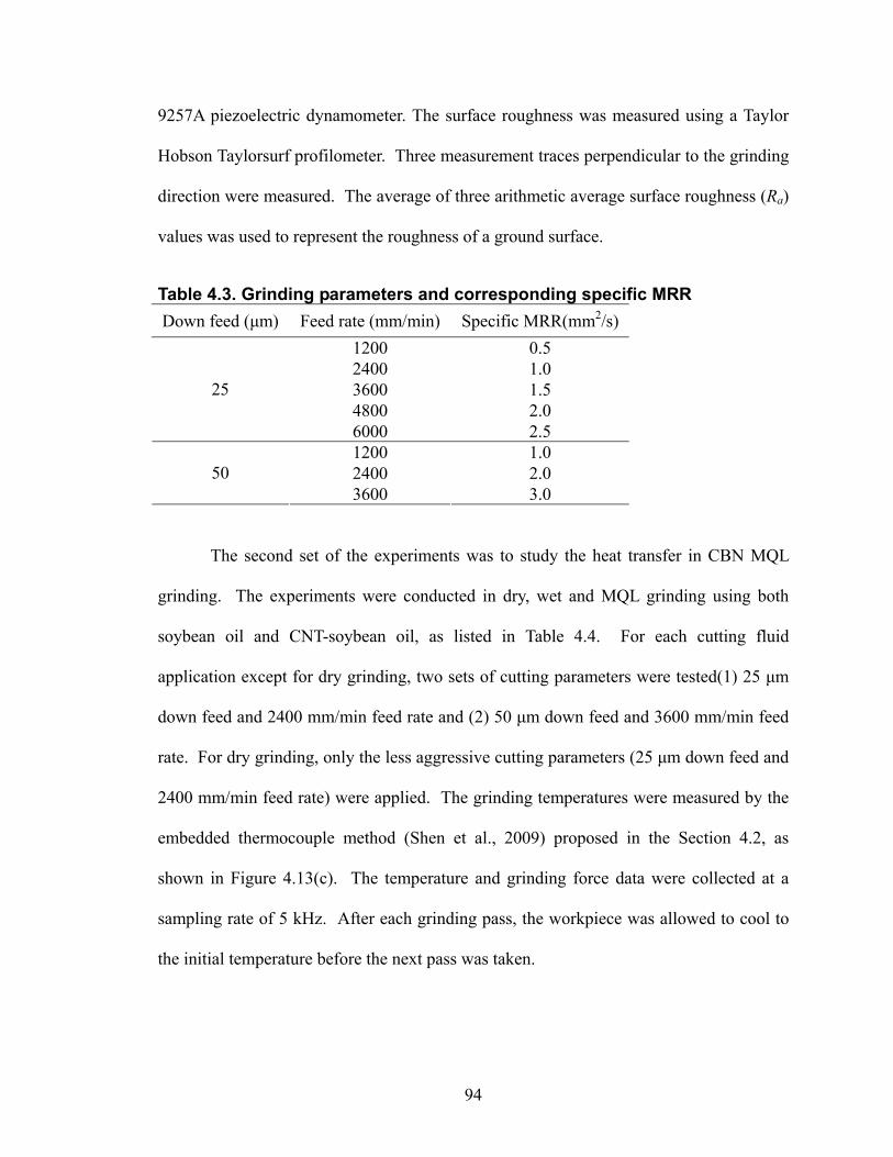
94

9257A piezoelectric dynamometer. The surface roughness was measured using a Taylor

Hobson Taylorsurf profilometer. Three measurement traces perpendicular to the grinding

direction were measured. The average of three arithmetic average surface roughness (Ra)

values was used to represent the roughness of a ground surface.

Table 4.3. Grinding parameters and corresponding specific MRR Down feed (μm) Feed rate (mm/min) Specific MRR(mm2/s)

1200 0.5 2400 1.0 3600 1.5 4800 2.0

25

6000 2.5 1200 1.0 2400 2.0 50 3600 3.0

The second set of the experiments was to study the heat transfer in CBN MQL

grinding. The experiments were conducted in dry, wet and MQL grinding using both

soybean oil and CNT-soybean oil, as listed in Table 4.4. For each cutting fluid

application except for dry grinding, two sets of cutting parameters were tested(1) 25 μm

down feed and 2400 mm/min feed rate and (2) 50 μm down feed and 3600 mm/min feed

rate. For dry grinding, only the less aggressive cutting parameters (25 μm down feed and

2400 mm/min feed rate) were applied. The grinding temperatures were measured by the

embedded thermocouple method (Shen et al., 2009) proposed in the Section 4.2, as

shown in Figure 4.13(c). The temperature and grinding force data were collected at a

sampling rate of 5 kHz. After each grinding pass, the workpiece was allowed to cool to

the initial temperature before the next pass was taken.

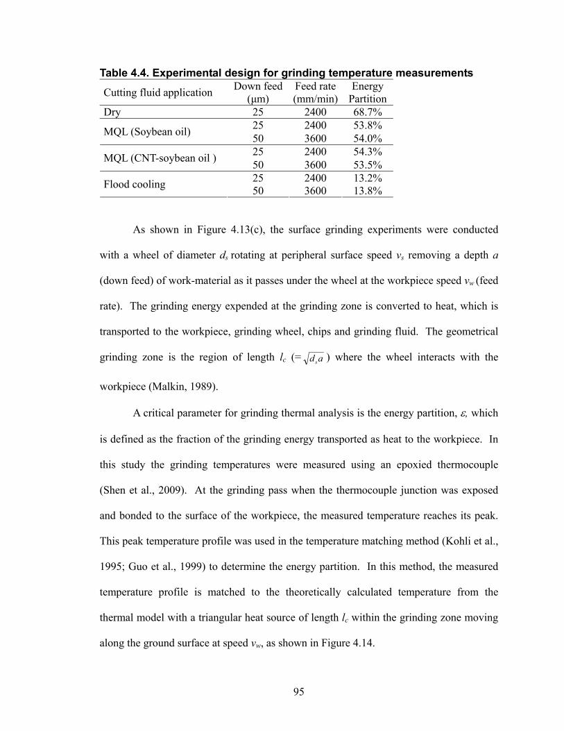
95

Table 4.4. Experimental design for grinding temperature measurements

Cutting fluid application Down feed (μm)

Feed rate (mm/min)

Energy Partition

Dry 25 2400 68.7% 25 2400 53.8% MQL (Soybean oil) 50 3600 54.0% 25 2400 54.3% MQL (CNT-soybean oil ) 50 3600 53.5% 25 2400 13.2% Flood cooling 50 3600 13.8%

As shown in Figure 4.13(c), the surface grinding experiments were conducted

with a wheel of diameter ds rotating at peripheral surface speed vs removing a depth a

(down feed) of work-material as it passes under the wheel at the workpiece speed vw (feed

rate). The grinding energy expended at the grinding zone is converted to heat, which is

transported to the workpiece, grinding wheel, chips and grinding fluid. The geometrical

grinding zone is the region of length lc (= ads ) where the wheel interacts with the

workpiece (Malkin, 1989).

A critical parameter for grinding thermal analysis is the energy partition, ε, which

is defined as the fraction of the grinding energy transported as heat to the workpiece. In

this study the grinding temperatures were measured using an epoxied thermocouple

(Shen et al., 2009). At the grinding pass when the thermocouple junction was exposed

and bonded to the surface of the workpiece, the measured temperature reaches its peak.

This peak temperature profile was used in the temperature matching method (Kohli et al.,

1995; Guo et al., 1999) to determine the energy partition. In this method, the measured

temperature profile is matched to the theoretically calculated temperature from the

thermal model with a triangular heat source of length lc within the grinding zone moving

along the ground surface at speed vw, as shown in Figure 4.14.

96

Figure 4.14 Schematic drawing of heat transfer in down grinding


The specific tangential and normal grinding force and force ratio vs. the specific

MRR for 25 μm down feed is shown in Figure 4.15. Both the normal and tangential

specific grinding forces increase almost linearly with respect to specific MRR. For the

specific tangential grinding force, although the amount of the cutting fluids was reduced

by about a thousand times, MQL grinding still has about the same tangential forces for all

tested conditions as compared to that of flood cooling. This is likely due to the good

lubrication of soybean oil as well as the more efficient penetration of the fluid into the

grinding zone by MQL delivery system (Silva et al., 2005). MQL grinding can achieve

the same level of MRR as that of flood cooling. It shows the potential feasibility of MQL

in high volume production grinding.

97

0

1

2

3

4

5

6

Spec

ific

tang

entia

l for

ce, F

t (N

/mm

)

Flood (Cimtech 500 )MQL (Soybean oil)MQL (CNT-soybean oil)

0

5

10

15

20

25

30

Spec

ific

norm

al fo

rce,

Fn

(N/m

m)

0.10

0.15

0.20

0.25

0.30

0.0 0.5 1.0 1.5 2.0 2.5 3.0

Specific MRR (mm2/s)

Forc

e ra

tio, F

t/Fn

Figure 4.15. Specific grinding forces vs. specific MMR (Down feed = 25 μm)

98

Adding CNT in soybean oil has no improvement in terms of the reduction in

grinding force. The previous study by Shen et al. (2008b) has pointed out that the

improvement of lubrication with nanoparticle additives could depend on the base fluid

chemistry which will guide their interaction (teaming) with the suspended nanoparticles.

The selection of appropriate base fluid is critical in the application of nano-lubricant. The

results of this study suggest that CNT as the additive lubricant is not appropriate for

soybean oil based fluid from the friction reduction point of view.

For specific normal grinding force, it is noticed that MQL grinding with pure

soybean oil and CNT-soybean oil has larger normal forces than that of flood cooling.

This is attributed to the larger viscosity of soybean oil, which results a higher hydraulic

pressure in the grinding zone. The higher normal grinding force and almost the same

tangential grinding force lead to a smaller Ft/Fn force ratio for MQL grinding. This

implies that better lubrication of the cutting fluid in MQL grinding.

The results of 50 μm down feed (seen in Figure 4.16) exhibited identical trend as

that of 25 μm down feed. At the same MMR, the specific tangential and normal grinding

forces of 50 μm down feed are slightly higher than that of 25 μm down feed. Larger

specific normal force was also observed in MQL grinding with soybean oil and CNT-

soybean oil compared to that of flood cooling.

99

0

1

2

3

4

5

6

7

8

Spec

ific

tang

entia

l for

ce, F

t (N

/mm

) Flood (Cimtech 500)MQL (Soybean oil)MQL (CNT-soybean oi)

0

5

10

15

20

25

30

35

40

Spec

ific

norm

al fo

rce,

Fn

(N/m

m)

0.10

0.15

0.20

0.25

0.30

0 1 2 3 4Specific MRR (mm2/s)

Forc

e ra

tio, F

t/Fn

(N/m

m)

Figure 4.16. Specific grinding forces vs. specific MMR (Down feed = 50 μm)

100

4.3.3. Surface Finish

The surface roughness results for 25 μm down feed are presented in Figure 4.17.

The surface roughness increases with the increasing feed rate, as is expected. Flood

cooling generate slightly better surface finish than that of MQL grinding, likely due to

better chip flushing to prevent scratching on the workpiece surface. The CNT additive

does not show improvement in terms of surface finish. The surface finish results of 50

μm down feed exhibited identical trend as that of 25 μm down feed, as shown in Figure

4.18.

0.20

0.21

0.22

0.23

0.24

0.25

0.26

0.27

0.28

0.29

0.30

0.0 0.5 1.0 1.5 2.0 2.5 3.0Specific MRR (mm2/s)

Ra

(μm

)

Flood (Cimtech 500)MQL (Soybean oil)MQL (CNT-soybean oil)

Figure 4.17. Surface finish results (Down feed = 25 μm)

101

0.20

0.21

0.22

0.23

0.24

0.25

0.26

0.27

0.28

0.29

0.30

0.0 1.0 2.0 3.0 4.0Specific MRR (mm2/s)

Ra

(μm

)

Flood (Cimtech)MQL (Soybean oil)MQL (CNT-soybean oil)

Figure 4.18. Surface finish results (Down feed = 50 μm)

4.3.4. Energy Partition

For dry grinding, the measured surface temperature profile vs. the dimensionless

distance, x/l, where x is the local coordinate described in Figure 4.14 and l=lc/2, is shown

in Figure 4.19. The experimental data matches perfectly with the theoretical temperature

for ε=68.7%. The good match validates the proposed grinding temperature measurement

and energy partition calculation.

Figures 4.20(a)-(c) present the temperature measurements in wet and MQL

grinding using both soybean oil and CNT-soybean oil under 25 μm down feed and 2400

mm/min feed rate. The measured temperature in wet grinding, as shown in Figure

4.20(a), is much lower and the energy partition ε=12.5%. Note there is significant

102

discrepancy of calculated and measured in the trailing edge (x/l <–1). It is due to the

fluid cooling effect. For MQL grinding, as shown in Figures 4.20(b) and (c), both

grinding temperature and energy partition are between the values of dry and wet grinding.

The temperature matching method gives ε=53.8% for MQL grinding using soybean oil

and ε=54.3% for CNT-soybean oil. The insignificant difference in ε shows the limited

effect of CNT additive. Even the thermal-physical properties of the MQL fluids can be

very different, it makes essentially no impact on the energy partition. Note that there is

also cooling effect due to fluid in the trailing edge (–5<x/l<–1) in MQL conditions. The

fluid flow rate in MQL grinding is very small so that only a small portion of the fluid is

able to pass through the grinding zone to cool the nearby trailing edge (–5<x/l<–1) of the

ground work-surface.

0

50

100

150

200

250

300

350

400

450

-20 -15 -10 -5 0 5Dimensionless distance, x/l

Tem

peat

ure

rise

(o C)

Experiment (Dry grinding)Theoretical ( = 68.7%)ε

a = 0.025 mmv w = 2400 mm/min

Figure 4.19. Temperature rise at the workpiece surface (dry grinding)

103

Figures 4.20(d)-(f) present the temperature measurements in wet and MQL

grinding using both soybean oil and CNT-soybean oil under 50 μm down feed and 3600

mm/min feed rate. Due to the limited spindle power, dry grinding is not feasible under

this grinding condition. The energy partition results are very similar to those under the

25 μm down feed and 2400 mm/min feed rate grinding condition. The measured

temperature in wet grinding, as shown in Figure 4.20(d), is relatively low and matches

with the theoretically calculated temperature for a much smaller ε=13.8%. Significant

cooling due to fluid in the trailing edge (x/l<–1) again is also evident, like in Figure

4.20(a). MQL grinding gives much higher temperature in this case due to the increased

grinding power, but the energy partition is almost the same as before, ε=54.0% for MQL

grinding using soybean oil and ε=53.5% for CNT-soybean oil.

The energy partition results are summarized in Table 4.4. About the same energy

partition values (67% for dry, 54% for MQL, and 14% for wet grinding) were observed,

regardless of the grinding parameter settings. This is consistent with the findings in

Varghese et al. (2000).

4.2.5. Summary

Grinding of cast iron using vitrified CBN wheels under dry, MQL and flood

cooling conditions was studied. Compared to the flood cooling condition, MQL grinding

could achieve the same MRR without increasing grinding forces. Flood cooling did

produce slightly better surface finish than MQL grinding due to efficient chip flushing.

The CNT additives showed no benefit to improve the grinding forces or surface finish.

104

0

10

20

30

40

50

60

70


Tem

peat

ure

rise

(o C)

Flood (Cimtech 500)Theoretical ( = 12.5%)ε

a = 0.025 mmv w = 2400 mm/min

Cooling due to fluid

(a)

0

20

40

60

80

100

120

140


Tem

peat

ure

rise

(o C)

Flood (Cimtech 500)Theoretical ( = 13.8%)ε

a = 0.05 mmv w = 3600 mm/min

Cooling due to fluid

(d)

0

50

100

150

200

250

300


Tem

peat

ure

rise

(o C)

MQL (Soybean oil)Theoretical ( = 53.8%)ε

a = 0.025 mmv w = 2400 mm/min

(b)

0

50

100

150

200

250

300

350

400

450

500


Tem

peat

ure

rise

(o C)

MQL (Soybean oil)Theoretical ( = 54.0%)ε

a = 0.05 mmv w = 3600 mm/min

(e)

0

50

100

150

200

250

300


Tem

peat

ure

rise

(o C)

MQL (CNT-soybean oil)Theoretical ( = 54.3%)ε

a = 0.025 mmv w = 2400 mm/min

(d)

0

50

100

150

200

250

300

350

400

450

500


Tem

peat

ure

rise

(o C)

MQL (CNT-soybean oil)Theoretical ( = 53.5%)ε

a = 0.05 mmv w = 3600 mm/min

(f) Figure 4.20. Temperature rise at the workpiece surface: (a), (b), (c) 25 μm down feed, 2400 mm/min feed rate, and (d), (e), (f) 50 μm down feed, 3600 mm/min feed rate.

105

Flood cooing condition had the lowest grinding temperature and smallest energy

partition of about 13%. The dry condition exhibited the highest grinding temperature and

largest energy partition of 68%. The energy partition under MQL condition is in between,

about 54%. These results are higher than the literature of CBN grinding. Varghese et al.

(2000) reported that values of the energy partition were found to range from 3 to 6% for

grinding of nodular cast iron with a vitrified CBN wheel in flood cooling condition, and

higher energy partitions up to 60% were obtained by reducing or eliminating the fluid.

The difference between our and Varghese et al. (2000) results is likely attributed to the

higher wheel surface speed (vs=60 m/s) used in their study. Based on the study by Lavine

(1988), high wheel speed reduces the energy partition and also enhance the forced

convection within the grinding zone by increasing the flow rate of the cutting fluid.

For conventional shallow-cut grinding of steels with Al2O3 wheels, measurement

of energy partition have been typically found to range from 60% to 85% (Malkin, 1989;

Kohli et al., 1995). Therefore, MQL grinding using vitrified CBN wheels with an energy

partition of about 54% is better than the conventional grinding with Al2O3 wheels in this

aspect.

Overall, this study shows that the vitrified CBN wheel can improve the

insufficient cooling problem of MQL grinding to certain extend. It is feasible to combine

MQL technique and vitrified CBN wheel to achieve high volume grinding production.

But, how to further increase the MRR without sacrifice of the surface finish or thermal

damage to the workpiece still needs more research. Advanced CBN wheel with more

porous vitreous bond is identified as a key technology to make the MQL CBN production

grinding possible.

106


A new thermocouple fixating method was developed for grinding temperature

measurement. Experiments were conducted to validate the proposed method. The

method was further used to experimentally investigate the heat transfer problems in

grinding. Grinding of cast iron using aluminum oxide and vitrified CBN wheels under

dry, MQL and flood cooling conditions was studied.

With conventional abrasive (aluminum oxide) wheels, grinding fluids provide

negligible cooling within the grinding zone as evidenced by the high energy partitions

which ranged from 84% to 92% for dry grinding, wet grinding, and MQL grinding. An

exception was observed for fine wet grinding which gave a much lower energy partition

of 24%, due to efficient cooling within the grinding zone below the film boiling

temperature. Cooling by the fluid was found to be more effective outside the grinding

zone rather than within the grinding zone.

With superabrasive wheels (vitrified CBN wheels), much lower energy partition

values were observed, about 68% for dry grinding, 54% for MQL grinding, and 13% for

wet grinding. It is concluded that the vitrified CBN wheel can improve the insufficient

cooling problem of MQL grinding to certain extend, and it is feasible to combine MQL

technique and vitrified CBN wheel to achieve high volume grinding production.

107

CHAPTER 5

GRINDING THERMAL MODEL BASED ON THE FINITE

DIFFERENCE METHOD

A grinding thermal model has been developed based on the finite difference

method (FDM) in order to estimate the energy partition and the convection heat transfer

coefficient in grinding. It also can be used to study the transient heat transfer and

temperature distributions in workpiece with finite dimension and various boundary

conditions. The model is first validated by comparing with the traditional grinding

thermal model assuming semi-infinite workpiece. Effects of workpiece size, feed rate,

and various cooling conditions are further investigated using the FDM model. When the

workpiece is short or the feed rate is low, transient heat transfer becomes more dominant

during grinding. Investigation of cooling effects revealed that the free convection and

cooling in the leading edge have negligible effect, cooling in the trailing edge only has

influence in the trailing edge region and cooling in the grinding zone has a significant

effect on the reduction of workpiece temperature. The model is further applied to

investigate convective cooling in the grinding experiment. The estimated average

convection heat transfer coefficient in the grinding contact zone was about 4.2×105

108

W/m2-K for wet grinding and 2.5×104 W/m2-K for MQL grinding, while the estimated

convection heat transfer coefficient in the trailing edge was much lower.

5.1. Introduction

The energy required to remove a unit volume of work-material for grinding is

very high. Virtually all this energy is converted to heat, which can cause high

temperatures and thermal damage to the workpiece such as grinding burn, phase

transformations, undesirable tensile residual tensile stresses, cracks, reduced fatigue

strength, thermal distortion and inaccuracies (Malkin, 1989). Workpiece thermal damage

is the major limitation to increase the material removal rate (MRR) in grinding.

A considerable research effort has devoted to both theoretical and experimental

aspects of heat transfer in grinding. The classic thermal analysis of moving heat source

and the temperature at sliding contacts was studied by Jaeger (1942). The application of

Jaeger’s moving heat source solutions to heat transfer problems in grinding was first

proposed by Outwater and Shaw (1952), whereby the grinding zone is approximated as a

band source of heat moving along the surface of the workpiece. Outwater and Shaw

(1952) assumed that grinding heat is mainly generated at the shear plane, and thus the

grinding temperature can be calculated by matching the average temperatures on the

shear plane. Hahn (1956) considered the frictional rubbing forces on the clearance

surface and neglected the cutting forces on the rake surface in the grinding thermal model.

Snoeys et al. (1979) and Malkin (1984) presented a comprehensive literature review of

early research work on the prediction of workpiece surface temperatures in dry grinding

without significant convective heat transfer.

109

Takazawa (1972) considered the partitioning of energy over the grinding contact

zone based on grinding wheel bulk thermal properties. Similar contact zone thermal

model was also proposed by Rowe et al. (1988). Shaw (1990) considered both real and

apparent contact areas, and used an area ratio factor to correlate grain properties with

such a model.

Grain analysis considers the energy partitioning at the grain-workpiece interface,

rather than the wheel-workpiece interface (the whole contact zone). It was first proposed

by Hahn (1956, 1962, 1966). Later, many grain analysis heat transfer models have been

developed (Liao et al., 2000; Maksoud, 2005). The grain analysis models tend to give

better results across a wide range of grinding conditions (Rowe et al., 1995).

Lavine (1988) developed an energy partition model, which combines both the

micro- and macro-scale thermal analysis. The wheel and grinding fluid are considered to

be a composite solid moving at the wheel speed. It predicts the convective heat transfer

coefficient on the workpiece surface, the fraction of energy entering the workpiece, and

the workpiece surface temperature. The model was further extended to account for the

variation of the heat fluxes along the grinding zone in down grinding with large Peclet

number (Jen and Lavine, 1995). Ju et al. (1998) considered both the scales of the wheel-

workpiece and grain-workpiece contact length and developed a complete thermal analysis

that can handle both up and down surface grinding without the assumption of large Peclet

number.

Temperature measurements in the workpiece subsurface during grinding indicated

that the triangular heat source is more accurate than the rectangular one (Kohli et al.,

1995). Analytical investigations by Guo and Malkin (1995a) indicated that energy

110

partition is approximately constant along the grinding zone for regular down grinding,

but varies greatly along the grinding zone for regular up grinding and both up and down

creep-feed grinding.

The inverse heat transfer method was also applied to grinding thermal modeling.

Guo and Malkin (1996a, 1996b) first developed an inverse heat transfer method to

estimate the heat flux distribution in the workpiece for regular grinding and the local

convective heat transfer coefficient on the workpiece surface from the measured

temperature distributions in the workpiece. Inverse heat transfer models have been

studied extensively in grinding processes (Hong and Lo, 2000; Wang and Chen, 2002;

Kim and Kwak, 2006). These models are similar to Guo and Malkin (1996a, 1996b),

except that Wang and Chen (2002) generalized the inverse heat transfer model to the 3D

case.

Most of these traditional grinding thermal models have assumptions such as the

steady-state condition, semi-infinite workpiece size, and adiabatic boundary condition on

the workpiece surface. The numerical method is an approach to overcome these

constraints. The finite element method (FEM) and finite difference method (FDM) are

considered to model the heat transfer problems in grinding. Guo and Malkin (1995b) has

developed the FDM based grinding thermal model for the transient temperature

distribution and shown that workpiece temperature rises rapidly during the initial wheel-

workpiece engagement, subsequently reaches a quasi-steady state value if the workpiece

is sufficiently long and further increases during the final wheel-workpiece disengagement.

The FEM has been widely employed to simulate the workpiece grinding temperature for

both 2D and 3D cases and further developed to analyze the phase transformation and

111

thermal stress on ground surface (Mahdi and Zhang, 1995; Biermann et al., 1997; Wang

et al., 2003; Mamalis et al., 2003; Lefebvre et al., 2006).

FDM applies the discrete analog of the derivative and is simple to formulate, easy

to apply and straightforward to extend to two or three dimensional problems. In this

study, a FDM based grinding thermal model is developed to study the heat transfer in

grinding. This model is similar to that developed by Guo and Malkin (1995b). In

addition to the transient heat transfer problem, this study also investigated the workpiece

with finite dimension and various boundary conditions. The model is introduced in

Section 2 and validated by comparing with the solution of the traditional heat transfer

model in Section 3. Effects of workpiece dimension, feed rate, and various boundary

conditions are studied using the FDM heat transfer model in Sections 4 and 5. In Section

6, the FDM heat transfer model is further applied in the grinding experiment to estimate

the energy partition and convection heat transfer coefficient.

5.2. Finite Difference Heat Transfer Model

To apply the finite difference method, the first step is to subdivide the

computation domain into small regions and assigning each region a reference point. In

this study, the computation domain is the workpiece, as shown in Figure 5.1(a). Each

node is at the center of a small region, and designated by the indices, as seen in Figure

5.1(b). The grid size is defined as the distance between the two adjacent nodes. In this

study, the uniform grid size is used, i.e., zx ΔΔ = . The moving heat source was assumed

to be triangular.

112

(a)

(b)

Figure 5.1. Illustration of nodal network: (a) mesh of the computation domain (workpiece) and (b) close-up view of the nodal network

5.2.1. Governing Equation

Now that the computation domain is characterized in terms of a nodal network,

the governing equation and the boundary conditions need to be transformed into the finite

difference form to compute the nodal temperatures. The 2D heat transfer governing

equation is:

tT1

zT

xT

2

2

2

2

∂∂

=∂∂

+∂∂

α (5.1)

Node (m, n)

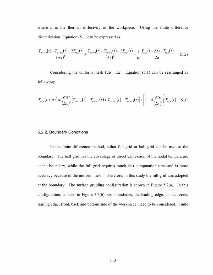
113

where α is the thermal diffusivity of the workpiece. Using the finite difference

discretization, Equation (5.1) can be expressed as:

( ) ( ) ( )( )

( ) ( ) ( )( )

( ) ( )t

tTttTz

tTtTtTx

tTtTtT nmnmnmnmnmnmnmnm

Δ−Δ+

=Δ

−++

Δ

−+ −+−+ ,,2

,1,1,2

,,1,1 122α

(5.2)

Considering the uniform mesh ( zx ΔΔ = ), Equation (5.1) can be rearranged as

following:

( )( )

( ) ( ) ( ) ( )[ ]( )

( )tTx

ttTtTtTtTx

tttT nmnmnmnmnmnm ,21,1,,1,12, 41 ⎥⎦

⎤⎢⎣

⎡Δ

Δ−++++

ΔΔ

=Δ+ +−+−αα

(5.3)

5.2.2. Boundary Conditions

In the finite difference method, either full grid or half grid can be used at the

boundary. The half grid has the advantage of direct expression of the nodal temperature

at the boundary, while the full grid requires much less computation time and is more

accuracy because of the uniform mesh. Therefore, in this study the full grid was adopted

at the boundary. The surface grinding configuration is shown in Figure 5.2(a). In this

configuration, as seen in Figure 5.2(b), six boundaries, the leading edge, contact zone,

trailing edge, front, back and bottom side of the workpiece, need to be considered. Finite

114

difference equations for these boundary conditions (BCs) can be derived by energy

conservation and the results are summarized in Appendix B.1.

(a)

(b)

Figure 5.2. Illustration of the boundary conditions: (a) surface grinding process and (b) the corresponding BCs

5.2.3. Surface Temperature

Since the full grid was used at the boundary instead of the half grid, the

temperature on the ground workpiece surface, Ts, which is of the most interest, needs to

be derived using energy balance method. Finite difference equations for the top surface

115

temperature prediction are presented in Appendix B.2.

5.3. Validation of Finite Different Thermal Model

Unlike the traditional grinding thermal models which only give the steady state

solution, the FDM heat transfer model can calculate the evolution of temperature within

the workpiece which makes it capable to handle the transient heat transfer problems in

grinding. To validate the FDM heat transfer model developed in this study, the results of

the FDM model is compared with the solution of the traditional heat transfer model

(Kohli et al, 1995; Guo and Malkin, 1996a; 1996b).

The FDM heat transfer model was first applied to simulate the spatial and

temporal temperature distribution of grinding Dura-Bar 100-70-02 ductile iron workpiece

with length L=50 mm and thickness H=10mm. The grinding parameters and work-

material properties are listed in Table 5.1. The triangular moving heat source, as shown

in Figure 5.2(b), with an average heat flux of 40 W/m2 and a width of contact length lc =

1.33 mm was used. All the BCs are set to be adiabatic, identical to the assumption for the

traditional heat transfer model.

Table 5.1. Summary of the parameters used in simulation Wheel diameter ds 177.8 (mm) Depth of cut a 10 (μm) Wheel speed, vs 30 (m/s) Feed rate, vw 0.04 (m/s) Thermal conductivity of workpiece, kw 63 (W/m·K) Thermal diffusivity of workpiece, αw 16.3×10-6 (m2/s)

The spatial distributions of temperature field in the workpiece at time t = 0.15,

0.40, 0.65, 0.90, and 1.15 (s) are shown in Figure 5.3. The time t = 0 s is defined at the

116

start of wheel contacting the workpiece. A similar pattern of the temperature field with

high temperature region of about 480°C is observed beneath the moving heat source and

propagating along the x-axis.

t=0.15 s

t=0.40 s

t=0.65 s

t=0.90 s

t=1.15 s

Figure 5.3. Temporal and spatial distributions of the workpiece temperature (L=50 mm and H=10 mm)

The temporal and spatial distributions of temperature on the ground surface are

plotted in Figure 5.4. There are three regions, cut-in, steady-state, and cut-out. In the

cut-in region, the workpiece peak temperature rises rapidly when the grinding wheel first

117

engages with the workpiece. In the steady-state region, the workpiece surface

temperature profile reaches a stable status. The peak temperature maintains at about

480°C, the same level of peak temperature in Figure 5.3. As the wheel disengaging from

the workpiece, due to the boundary condition, the peak temperature increases to 550°C

and higher for a short period of time in the cut-out region. The transient heat transfer

during the cut-in and cut-out region has been previously studied by Guo and Malkin

(1995b). This simulation results also indicate that a steady-state region exists if the

workpiece is long enough.

0 10 20 30 40 50050

100150200250300350400450500550600650

x (mm)

Tem

pera

ture

rise

(o C)

Cut-In Steady-StateCut-Out

t=0.07 st=0.45 s t=0.85 s t=1.24 s

Figure 5.4. Temporal and spatial distribution of the grinding temperature at the workpiece surface (L=50 mm, H=10 mm, vw=2400 mm/min)

The steady-state FDM heat transfer solution is compared with that of the

traditional heat transfer model. As shown in Figure 5.5, the FDM surface temperature

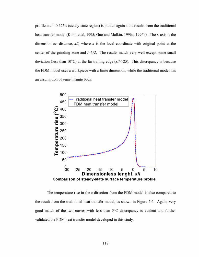
118

profile at t = 0.625 s (steady-state region) is plotted against the results from the traditional

heat transfer model (Kohli et al, 1995; Guo and Malkin, 1996a; 1996b). The x-axis is the

dimensionless distance, x/l, where x is the local coordinate with original point at the

center of the grinding zone and l=lc/2. The results match very well except some small

deviation (less than 10°C) at the far trailing edge (x/l<-25). This discrepancy is because

the FDM model uses a workpiece with a finite dimension, while the traditional model has

an assumption of semi-infinite body.

-30 -25 -20 -15 -10 -5 0 5 100

50

100

150

200

250

300

350

400

450

500

Dimensionless lenght, x/l

Tem

pera

ture

rise

(o C)

Traditional heat transfer modelFDM heat transfer model

Comparison of steady-state surface temperature profile

The temperature rise in the z-direction from the FDM model is also compared to

the result from the traditional heat transfer model, as shown in Figure 5.6. Again, very

good match of the two curves with less than 5°C discrepancy is evident and further

validated the FDM heat transfer model developed in this study.

119

0 1 2 3 4 5 6 7 8 9 100

50

100

150

200

250

300

350

400

450

500

z (mm)

Tem

pera

ture

rise

(o C)

Traditional heat transfer modelFDM heat transfer model

Figure 5.6. Comparison of temperature rise along the z-direction (at x/l=0)

5.4. Effects of Workpiece Dimension and Workpiece Velocity

5.4.1. Effect of Workpiece Length

As discussed in the previous session, when the workpiece is long, a steady state

region exists. However, if the workpiece is short, the whole process would become a

transient heat transfer problem. An example when the length of the workpiece in Sec. 3

is shortened to 5 mm (same thickness H = 10 mm) is shown in Figure 5.7. The peak

temperature at the workpiece surface continues going up until the grinding wheel

disengages with the workpiece. No steady state can be reached during the whole process.

120

0 1 2 3 4 50

100

200

300

400

500

600

700

x (mm)

Tem

pera

ture

rise

(o C)

t=0.01 s

t=0.02 s

t=0.03 s

t=0.04 st=0.05 s

t=0.06 s

t=0.07 st=0.08 s

t=0.09 s

t=0.10 s

t=0.11 s

t=0.12 s

Figure 5.7. Effect of workpiece length (L=5 mm, H=10 mm, vw=2400 mm/min)

5.4.2. Effect of Workpiece Thickness

The thickness of the workpiece mainly affects the temperature rise along the z-

direction in the workpiece. The distribution of steady-state grinding surface temperature

in the z-direction for H = 1, 2, 5, and 10 mm and L = 50 mm is shown in Figure 5.8.

Compared to the traditional heat transfer model which assumes semi-infinite workpiece

size, the temperature profile of H = 10 mm matches very well. When the workpiece is

thick enough, H > 5 mm, the FDM solution is almost identical to the result from the

traditional heat transfer model. The discrepancy starts to show when H < 2 mm. Also,

the thinner workpiece has higher surface temperature because the heat cannot be

dissipated efficiently in the z-direction.

121

0 0.5 1.0 1.5 2.0 2.5 3.0-500

50100150200250300350400450500550

z (mm)

Tem

pera

ture

rise

(o C)

Traditional Heat Transfer ModelFDM Heat Transfer Model (H = 10 mm)FDM Heat Transfer Model (H = 5 mm)FDM Heat Transfer Model (H = 2 mm)FDM Heat Transfer Model (H = 1 mm)

Figure 5.8. Effect of workpiece thickness (L=50 mm, vw=2400 mm/min)

5.4.3. Effect of Workpiece Velocity

The workpiece velocity (feed rate) vw has the same effect as the length of the

workpiece. For example, as shown in Figure 5.9, under the same workpiece size (L = 50

mm and H = 10 mm), when vw is small (vw=240 mm/min), the transient heat transfer may

become dominant during the whole process, and the temperature is also much higher due

to the prolonged period for the heat conduction.

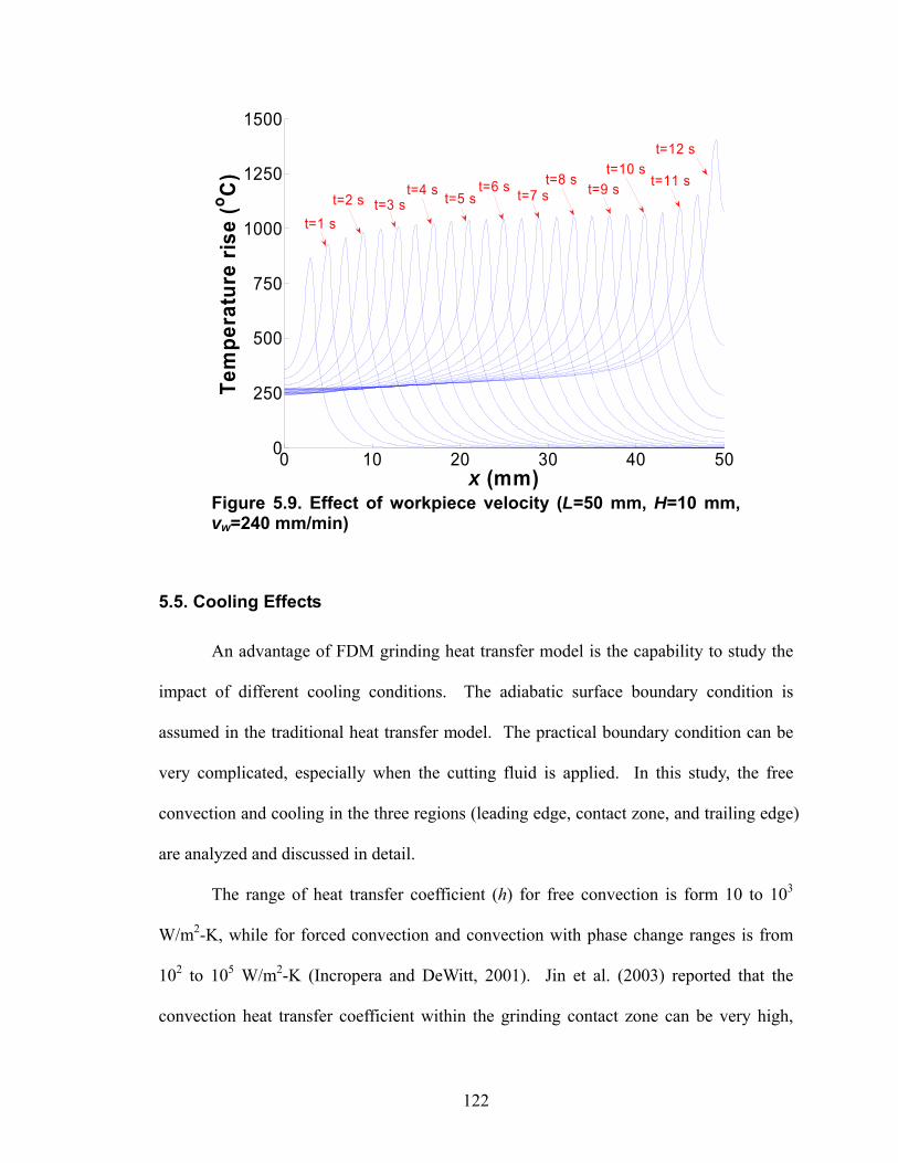
122

0 10 20 30 40 500

250

500

750

1000

1250

1500

x (mm)

Tem

pera

ture

rise

(o C)

t=3 st=1 s

t=5 s t=7 s t=9 st=6 st=4 st=2 s

t=8 st=10 s

t=11 s

t=12 s

Figure 5.9. Effect of workpiece velocity (L=50 mm, H=10 mm, vw=240 mm/min)

5.5. Cooling Effects

An advantage of FDM grinding heat transfer model is the capability to study the

impact of different cooling conditions. The adiabatic surface boundary condition is

assumed in the traditional heat transfer model. The practical boundary condition can be

very complicated, especially when the cutting fluid is applied. In this study, the free

convection and cooling in the three regions (leading edge, contact zone, and trailing edge)

are analyzed and discussed in detail.

The range of heat transfer coefficient (h) for free convection is form 10 to 103

W/m2-K, while for forced convection and convection with phase change ranges is from

102 to 105 W/m2-K (Incropera and DeWitt, 2001). Jin et al. (2003) reported that the

convection heat transfer coefficient within the grinding contact zone can be very high,

123

about 290,000 W/m2-K for the water-based cutting fluid and 23,000 W/m2-K for oil-

based cutting fluid. In this study, h is assumed to range from 10 to 103 W/m2-K for free

convection condition and 103 to 105 W/m2-K for forced convection and convection with

phase change. All the other parameters used in this section are the same as in Table 5.1.

5.5.1. Free Convection

Figure 5.10 shows the steady-state surface temperature profiles for the whole

surface (leading edge, contact zone, and trailing edge) under the adiabatic and free

convection (h = 10, 102, and 103 W/m2-K) boundary conditions. The results with free

convection are almost identical to that with adiabatic boundary condition. This indicates

that the free convection is not strong enough to influence the heat transfer in the grinding

process.

-12 -10 -8 -6 -4 -2 0 2 4 60

50

100

150

200

250

300

350

400

450

500

Dimensionless lenght, x/l

Tem

pera

ture

rise

(o C)

Adiabatichfree convection=10 W/m2-K

hfree convection=102 W/m2-K

hfree convection=103 W/m2-K

Figure 5.10. Effect of free convection (surface temperature)

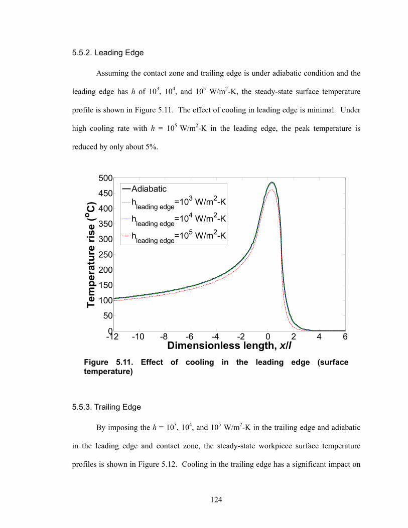
124

5.5.2. Leading Edge

Assuming the contact zone and trailing edge is under adiabatic condition and the

leading edge has h of 103, 104, and 105 W/m2-K, the steady-state surface temperature

profile is shown in Figure 5.11. The effect of cooling in leading edge is minimal. Under

high cooling rate with h = 105 W/m2-K in the leading edge, the peak temperature is

reduced by only about 5%.

-12 -10 -8 -6 -4 -2 0 2 4 60

50

100

150

200

250

300

350

400

450

500

Dimensionless length, x/l

Tem

pera

ture

rise

(o C)

Adiabatichleading edge=103 W/m2-K

hleading edge=104 W/m2-K

hleading edge=105 W/m2-K

Figure 5.11. Effect of cooling in the leading edge (surface temperature)

5.5.3. Trailing Edge

By imposing the h = 103, 104, and 105 W/m2-K in the trailing edge and adiabatic

in the leading edge and contact zone, the steady-state workpiece surface temperature

profiles is shown in Figure 5.12. Cooling in the trailing edge has a significant impact on

125

the temperature profile. But it only influences the trailing edge, not the contact zone or

the leading edge. The peak temperature remains about the same as that with high h in

trailing edge cooling.

-12 -10 -8 -6 -4 -2 0 2 4 60

50

100

150

200

250

300

350

400

450

500


Tem

pera

ture

rise

(o C)

Adiabatichtrailing edge=103 W/m2-K

htrailing edge=104 W/m2-K

htrailing edge=105 W/m2-K

Figure 5.12. Effect of cooling in the trailing edge (surface temperature)

5.5.4. Contact Zone

For h = 103, 104, and 105 W/m2-K in the grinding contact zone and adiabatic in the

leading and trailing edges, the corresponding steady-state workpiece surface temperature

profile is shown in Figure 5.13. Efficient cooling in the grinding contact zone has a

significant impact on the peak temperature and trailing edge temperature. This

observation confirms that the contact zone cooling is the most dominant factor in

grinding.

126

-12 -10 -8 -6 -4 -2 0 2 4 60

50

100

150

200

250

300

350

400

450

500


Tem

pera

ture

rise

(o C)

Adiabatichcontact zone=103 W/m2-K

hcontact zone=104 W/m2-K

hcontact zone=105 W/m2-K

Figure 5.13. Effect of cooling in the contact zone (surface temperature)

5.6. Energy Partition Prediction

In this section, the FDM heat transfer model was used to estimate the energy

partition (ratio of the energy entering the workpiece) in the real grinding application. The

FDM heat transfer model traces the temporal distribution of the temperature in the

workpiece, rather than only gives a steady-state solution. Therefore, the temperature

response measured by the thermocouple, which is in the time domain, can be directly

matched to the results calculated from the FDM heat transfer model. This makes the

FDM advantageous when the grinding process is unable to reach the steady-state

condition under the circumstance of short workpiece, slow vw, and others.

According to the results in Chapter 4, the energy partition for the vitrified CBN

wheel is estimated as 68% for dry grinding, 54% for MQL grinding, and 13% for wet

127

grinding (Shen and Shih, 2009), as summarized in Table 5.2. These values were

calculated based on the traditional heat transfer model, which has already considered the

cooling within the grinding zone. The reduced energy partition values in MQL and wet

grinding are attributed to the convection cooling of fluids in the grinding zone. However,

the traditional heat transfer model is unable to estimate the convection heat transfer

coefficient in the grinding process.

Table 5.2. Grinding parameters and corresponding energy partition results

Cutting fluid application Flowrate (ml/min)

Depth of cut (μm)

Feed rate (mm/min)

Energy partition(εdry or εfluid)

Dry -- 68.7% MQL (soybean oil) 5 53.8% Wet (5 vol% Cimtech 500 synthetic grinding fluid) 5400

25 2400 13.2%

Inputs for the FDM heat transfer model, as presented in Section 4.3, has 177.8

mm in diameter for vitreous bond CBN grinding wheel, 30 m/s wheel surface speed (vs),

Dura-Bar 100-70-02 ductile iron work-material, 63 W/m-K thermal conductivity,

1.63×10-7 m2/s thermal diffusivity, and 57 mm long, 6.5 mm wide and 20 mm tall

workpiece.

The total heat flux (qtotal) is assumed to be partitioned between the grinding wheel

(qwheel) and workpiece/fluid (qwf).

cw

stwfwheeltotal lb

vFqqq =+= (5.16)

where Ft is the tangential grinding force and bw is the width of the workpiece. In dry

grinding, there is no heat flux carried away by the cutting fluids; therefore,

128

totaldryworkpiecewf qqq ε== (5.17)

In wet or MQL grinding, the heat flux enters both workpiece and fluids; thus,

fluidtotalfluidfluidworkpiecewf qqqqq +=+= ε (5.18)

where εdry and εfluid are the energy partition into the workpiece under dry and wet/MQL

condition, respectively.

The energy partition values in Table 5.2 were estimated by temperature matching

method using the traditional heat transfer model (Kohli et al., 1995). The same results

with less than 0.1% discrepancy can also be obtained using the proposed FDM heat

transfer model by imposing the adiabatic BCs, as shown in Figure 5.14. The only

difference is that the temperature matching was done in the time domain instead of in the

space domain.

In Figures 14(b) and (c), the deviation from the experimental measurements and

FDM results is evident under the wet and MQL conditions due to the assumption of

adiabatic BCs. This problem can be solved by using the appropriate boundary conditions.

The FDM heat transfer model is further developed in the next section to estimate the

convection heat transfer coefficient in the grinding process.

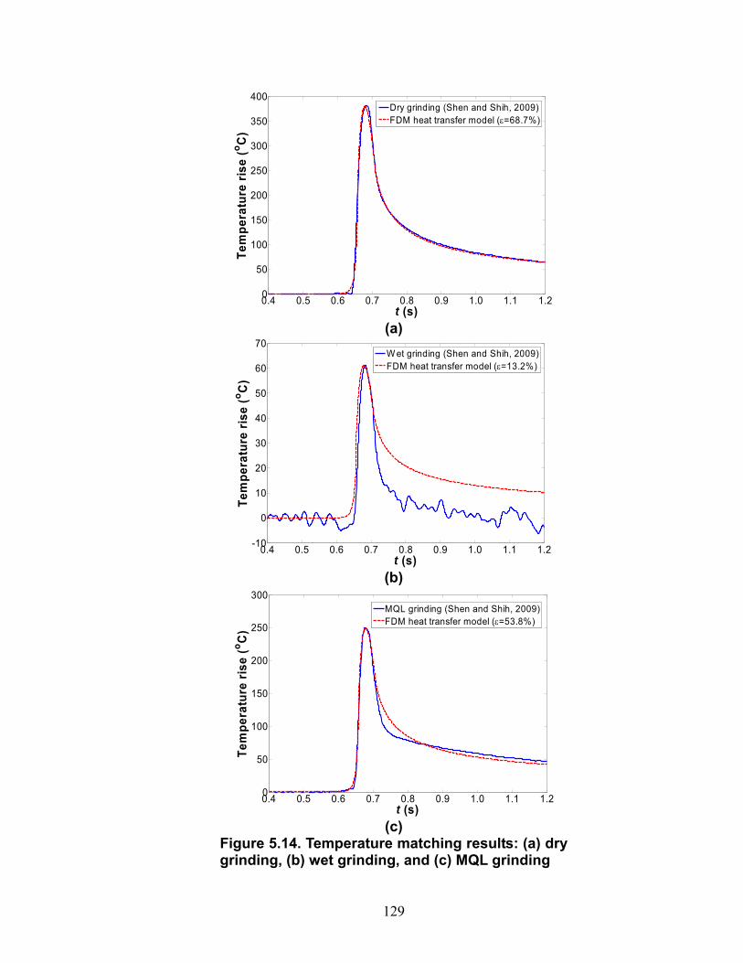
129

0.4 0.5 0.6 0.7 0.8 0.9 1.0 1.1 1.20

50

100

150

200

250

300

350

400

t (s)

Tem

pera

ture

rise

(o C)

Dry grinding (Shen and Shih, 2009)FDM heat transfer model (ε=68.7%)

(a)

0.4 0.5 0.6 0.7 0.8 0.9 1.0 1.1 1.2-10

0

10

20

30

40

50

60

70

t (s)

Tem

pera

ture

rise

(o C)

W et grinding (Shen and Shih, 2009)FDM heat transfer model (ε=13.2%)

(b)

0.4 0.5 0.6 0.7 0.8 0.9 1.0 1.1 1.20

50

100

150

200

250

300

t (s)

Tem

pera

ture

rise

(o C)

MQL grinding (Shen and Shih, 2009)FDM heat transfer model (ε=53.8%)

(c)

Figure 5.14. Temperature matching results: (a) dry grinding, (b) wet grinding, and (c) MQL grinding

130

5.7. Convection Heat Transfer Coefficient Prediction

Assuming the energy partition to the workpiece/fluid is the same in dry, wet and

MQL grinding, i.e., totaldrywf qq ε= regardless of the cooling condition. Thus, as long as

εdry is known, the heat flux input qwf for the FDM heat transfer model can be found. In

addition, the heat flux into the cutting fluid can be expressed as:

( ) ( )[ ]∫−−=

l

l as

fluid dxTxTxhq (5.19)

where Ta is the fluid (or ambient) temperature.

The actual depth of cut in the grinding zone decreases from the leading edge side

to the trailing edge side for down grinding. This creates the non uniform convective

cooling. As shown in Figure 5.15, in this study the convection heat transfer coefficient in

the grinding zone, hcontact, is assumed as a linear function.

( ) ⎟⎠⎞

⎜⎝⎛ +

−+=

212

1c

ccontact

lxl

hhhxh (5.20)

where ( )[ ]xhmaxh contact=2 , ( )[ ]xhminh contact=1 , and x is the local coordinate with original

point at the center of the grinding zone. The average convection heat transfer coefficient

in the grinding zone, contath is defined as:

2

21 hhhcontat+

= (5.21)

131

Figure 5.15. Assumption of convection heat transfer coefficient

The convection heat transfer coefficient in the trailing edge, htrailing, is assumed to

be uniform. Due to the continuity constraint, the convection heat transfer coefficient

should not change rapidly between the trailing edge and the end of the contact zone at x =

−l, where the actual depth of cut is close to zero. Therefore,

1hhtrailing = (5.22)

According to Section 5, cooling effect in the leading edge is negligible. Hence

BCleading_edge is set to be adiabatic. The other three boundaries, BCback, BCfront, and

132

BCbottom, are also set to be adiabatic. A triangular heat source with an average heat flux of

qwf was used.

By matching the measured temperature profile to the calculated temperature from

the FDM heat transfer model, the convection heat transfer coefficient within the grinding

zone ( contacth ) and in the trailing edge (htrailing) can be found. The temperature matching

results are shown in Figure 5.16, and the estimated convection heat transfer coefficient

values are summarized in Table 5.3. The convection heat transfer coefficient in the

contact zone is much higher than that in the trailing edge for all cases. This is expected

because of the much higher fluid velocity in the contact zone. Wet grinding has much

higher convection heat transfer coefficient than MQL grinding both in the contact zone

and the trailing edge.

Table 5.3. Summary of convection heat transfer coefficient

Cutting fluid application 2h (W/m2-K)

contacth (W/m2-K)

trailingh (W/m2-K)

MQL (soybean oil) 3.9 × 104 2.5 ×104 1.0 × 104 Wet (5 vol% Cimtech 500 synthetic grinding fluid) 7. 4 × 105 4.2 × 105 9.5 × 104

As shown in Figure 5.16(a), for wet grinding, the uniform convection heat

transfer coefficient in the trailing edge gives very good matching. However, for MQL

grinding, as seen in Figure 5.16(b), the convection heat transfer coefficient in the trailing

edge may not be uniform. The calculated temperature profile with a high htrailing matches

with the experimental measurement very well in the trailing edge near the contact zone,

but not in the trailing edge far away from the contact zone, while the calculated

temperature profile with a zero htrailing has the opposite result. It indicated that MQL only

provided some cooling in the trailing edge near the contact zone. This is probably due to

133

the low flow rate in MQL grinding which only allows a small portion of the fluid to pass

through the grinding zone and cool the nearby trailing edge of the ground surface;

however, in the trailing edge far away from the contact zone, MQL provides no cooling.

0.4 0.5 0.6 0.7 0.8 0.9 1.0 1.1 1.2-10

0

10

20

30

40

50

60

70

80

t (s)

Tem

pera

ture

rise

(o C)

W et grinding (Shen and Shih, 2009)FDM heat transfer model

htrailing=9.5x104 W /m2-K

hcontact=4.2x105 W /m2-K

(a)

0.4 0.5 0.6 0.7 0.8 0.9 1.0 1.1 1.20

50

100

150

200

250

300

350

t (s)

Tem

pera

ture

rise

(o C)

MQL grinding (Shen and Shih, 2009)FDM heat transfer model (htrailing=1.0x104 W /m2-K)FDM heat transfer model (htrailing=0)

hcontact=2.5x104 W /m2-K

htrailing=1.0x104 W /m2-K

htrailing=0

(b)

Figure 5.16. Convection heat transfer coefficient prediction: (a) wet grinding and (b) MQL grinding

134


A FDM based grinding thermal model was developed and validated by comparing

with the traditional heat transfer model. The FDM heat transfer model was used to study

the effects of workpiece size, workpiece velocity (feed rate), and cooling in the leading

edge, trailing edge and grinding zone. Transient heat transfer occurred in the cut-in and

cut-out regions. When the workpiece was short or the feed rate was low, the transient

effect was more significant. The thickness of the workpiece could influence the

temperature profile along the z-direction in the workpiece. As for cooling effects, the free

convection and cooling in the leading edge were neglectable; the convection heat transfer

in the trailing edge could not reduce the peak temperature; and the most efficient cooling

was in the grinding contact zone.

The FDM heat transfer model was further applied in the grinding experiment to

estimate the energy partition and convection heat transfer coefficient. By imposing the

adiabatic boundary conditions, the model was capable to estimate the same energy

partition values as the traditional heat transfer model. The estimated average convection

heat transfer coefficient in the grinding zone was about 4.2×105 W/m2-K for wet grinding

and 2.5×104 W/m2-K for MQL grinding. The convection heat transfer coefficient in the

trailing edge was about an order of magnitude lower than that in the grinding contact

zone. However, MQL only provides some cooling in the trailing edge near the contact

zone. In addition, a uniform convection heat transfer in the trailing edge may not be

realistic for MQL grinding. More complicated cooling boundary conditions needs to be

investigated and the FDM heat transfer model needs to be further improved.

135

CHAPTER 6

CONCLUSIONS AND FUTURE WORK

This research advances the fundamental research of nanofluids and the state-of-

the-art MQL grinding. The formulation and characterization of nanofluids, and MQL

grinding of cast iron using nanofluids were investigated. A new thermocouple fixating

method for grinding temperature measurement was proposed, thermal analysis of MQL

grinding was conducted, and a grinding thermal model based on the Finite Difference

Method has been developed.

6.1. Major Contributions

The major contributions made in this research include:

1. The fundamental research of nanofluids was conducted. The suspension of

nanoparticles has been proved to be able to enhance the thermal conductivity,

especially with the high volume fraction of nanoparticles. Although the

nanofluids showed higher Nusselt number than the base fluid at the same

Reynolds number; in terms of convection heat transfer coefficient vs. flow rate,

136

there is no significant difference between the nanofluids and the base fluid.

2. The application of nanofluids in MQL grinding was evaluated for the first time. It

is concluded that nanofluids are not able to provide superior cooling capacity in

MQL grinding process. However, the suspension of nanoparticles can improve

the tribological properties of the base fluids, which can help lubricate the grinding

zone. Therefore, the research of application of nanofluids in MQL grinding

should focus on the advanced lubrication properties.

3. It is shown for the first time that lubricant oils with novel MoS2 nanoparticles

significantly reduces the tangential grinding force and friction between the wear

flats and the workpiece, increases G-ratio and improves the overall grinding

performance in MQL applications.

4. A new thermocouple fixating method was developed for grinding temperature

measurement which is easy to install, and can provide a direct measurement of the

surface temperature.

5. Thermal analysis for MQL grinding was studied for the first time. For shallow-

cut grinding of cast iron using a vitreous bond aluminum oxide wheel, the energy

partition was estimated as 84% for dry grinding, 84% for MQL grinding, but only

24% for wet grinding due to cooling within the grinding zone below the film

boiling temperature.

6. Much lower energy partition to the workpiece (68% for dry grinding, 54% for

MQL grinding, and 13% for wet grinding) was achieved by using vitrified bond

CBN wheel. The insufficient cooling problem of MQL grinding can be improved

by using the vitrified CBN wheel, which makes the MQL grinding feasible in the

137

high volume production.

7. A grinding thermal model has been developed based on the Finite Difference

Method to better understand the transient heat transfer and temperature

distributions in workpiece with finite dimension and various cooling conditions.

8. The FDM heat transfer model was applied to estimate the convection heat transfer

coefficient in grinding. The average convection heat transfer coefficient in the

contact zone was about 4×105 W/m2-K for wet grinding and 2×104 W/m2-K for

MQL grinding, while the convection heat transfer coefficient in the trailing edge

is much lower.

Overall, the research included the fundamental research of nanofluids, evaluation

of grinding performance, measurement of grinding temperature, thermal analysis and

FDM heat transfer modeling of the grinding process. It has showed that the key to the

success of MQL grinding is (1) the grinding fluid with advanced tribological properties,

(2) the grinding wheel with high thermal conductivity, and (3) the good understanding of

cooling effects in grinding processes. The first point can be achieved by the development

of new type of nanofluids which contains the nanoparticles with advanced lubricity. The

second can be achieved using superabrasive grinding wheels such as CBN wheels. And

the last has been addressed by the methodology developed in this study.

6.2. Recommendations for Future Study

This study has identified several future directions for the development of

engineering nanofluids and MQL grinding:

138

The mechanism of enhanced thermal conductivity for nanofluids is still not clear.

Fundamental research needs to be continued in order to better understand the involved

mechanism. This is the foundation of the future nanofluids research, which can be used

to guide the formulation of nanofluids for cooling application.

The mechanism of enhanced lubricating properties for nanofluids needs to be

further explored. The experimental results have shown that the improvement of

lubrication with lubricating nanoparticle additive could depend on the base fluid

chemistry. Thus the selection of appropriate base fluid is very critical in the application

of nanoparticle based lubricants in MQL grinding and requires further course of research

in this field.

Based on the better understanding of nanofluids, future researches can be

conducted on formulation of new nanofluids to achieve excellent tribological and thermal

properties, and explore the feasible industrial application such as engine/fuel

cell/radiator/ power electronics cooling and MQL machining.

It has been shown that MQL grinding using vitrified CBN wheels is very

promising for the high volume grinding production. Therefore, the process needs to be

further optimized.

In addition, the dimension accuracy of the ground parts has not been addressed in

this study. It is another big concern for manufacturing production; especially with MQL,

the accumulated heat can cause large thermal expansion of the workpiece, resulting in

thermal distortion and inaccuracies. Workpiece dimension accuracy for MQL machining

has already been studied (Braga et al., 2002; Furness et al., 2006; Dhar et al., 2007), but

not in MQL grinding, which definitely needs more investigation.

139

Chip flushing seems to be a major concern for MQL grinding, resulting in

undesired surface finish of ground parts. This problem has to be addressed before the

MQL technology can be applied to the grinding production. One possible solution is to

design a chip cleaning sub-system such as vacuum suction or high pressure air blow, as a

supplement to the MQL delivery system.

The Finite Difference Method based heat transfer model developed in this

research has been proved to be a simple and powerful tool to conduct the thermal analysis

of the grinding process. It needed to be further improved to be more accurate and more

comprehensive. For example, more complicated cooling boundary conditions and

grinding zone geometry (especially for creep grinding) can be introduced into the FDM

heat transfer model.

Each of these suggested future topics can be used to further enhance the

understanding of nanofluids and contribute to the development of environmentally benign

MQL grinding processes.

140

APPENDICES

141

Appendix A

Characterization of Nanofluids

The thermal properties of nanofluids including thermal conductivity and

convection heat transfer coefficient are studied in this research.

A.1. Thermal Conductivity Measurements

A.1.1. Transient Hot Wire Method

Transient hot wire method is widely used to measure thermal conductivity of

materials, especially for fluids. It was developed about thirty years ago (DeGroot et al.,

1974; Castro et al., 1976; Nagasaka and Nagashima, 1981; Hoshi et al., 1981). Before

that time, the thermal conductivity of fluids had historically proven to be a difficult

transport property to measure accurately because the heat transfer by convection was

recognized as a prominent source of error during the measurement (DeGroot et al., 1974).

The most advantageous feature of the transient hot wire method for thermal conductivity

measurements of fluids is its capability of experimentally eliminating convective error,

and for this reason, it is a high precision technique for the measurement of the thermal

conductivity of fluids (Nagasaka and Nagashima, 1981).

The theory of the transient hot wire method was developed in Carslaw and Jaeger

142

(1959). Based on the model of a perfectly conducting line heat source of infinite length

surrounded by an infinite medium, the temperature rise of the heater wire, T, as a function

of time, t, is given by (Batty et al., 1981):

⎥⎦

⎤⎢⎣

⎡−⎟

⎠⎞

⎜⎝⎛= γα

π 2

4ln4

)(r

tk

qtT (A.1)

where r is the radius of the heater wire; q is the heat dissipated per unit length, α and k

are the thermal diffusivity and thermal conductivity of the fluid to be tested; and γ is

Euler's constant.

Equation (A.1) is subjected to the following assumptions:

1) The radius r of the wire is infinitesimal and the length is infinite.

2) The surrounding medium is infinite.

3) The temperature in the wire is uniform.

4) Heating period is long enough, that is, Fourier number, Fo >> 1, i.e.

120 >>=r

tF α (A.2)

The first two assumptions are hard to achieve under real engineering conditions.

Thus, the effects of departures from ideal conditions on the accuracy of the thermal

conductivity determinations had been studied. To avoid significant errors due to the

effect of heater wire being finite, Blackwell (1954) proposed the minimum probe length

to radius ratio, that is

2/10

0632.0⎟⎠⎞

⎜⎝⎛>

FrL (A.3)

143

where L is the length of the wire.

Vos (1955) concluded that the effect of test medium being finite, i.e. the boundary

effects, become significant if

6.042 >

btα (A.4)

where b represents the shortest distance between the heater wire and the nearest boundary

of the test medium.

Equation (A.1) can also be rewritten as (Batty et al., 1981):

( )tk

qtT ln4

)( Δ=Δπ

(A.5)

Therefore, the curve of temperature, T, versus time, t, on a semi-log plot is a

linear line, and the slope of this line is q/4πk. Thus, if the heat flux q is known, the

thermal conductivity of the test fluid can be determined experimentally by monitoring the

wire temperature.

In practice, it is easy to measure the temperature of the heater wire if it is made of

platinum since its resistance-temperature is well-established and measurement of

resistance is much easier than measurement of temperature. For the range 0 to 630ºC,

Callendar equation gives (Lowenthal and Harper, 1960):

( )21)0()( bTaTRTR ++= (A.6)

where R(T) is the resistance of the platinum wire at temperature, T and R(0) is the

resistance of the platinum wire at 0ºC; a and b are Callendar-Van Dusen coefficients.

144

According to ASTM Standards E 1137, a=3.9083× 10-3 (ºC-1) and b= 5.775 × 10-7 (ºC -2).

A.1.2. Experimental Setup

The thermal conductivity measurement apparatus, as shown in Figure A.1, was

built based on transient hot wire method described in Section A.1.1. Two hot platinum

wire probes, 76 μm in diameter, were developed. One probe is made of a long wire (200

mm long), as shown in Figure A.1(a) and the other probe has a short platinum wire (20

mm long), as shown in Figure A.1(b). The short wire probe is particularly suitable to test

nanofluids because only a small amount of fluid is required. Both platinum wires are

coated with thin Teflon film for electrical insulation. As shown in Figure A.1(c), the hot

wire probe is inserted in a tube with inner diameter of 22.1 mm. The tube is filled with

test fluid so that the platinum wire is submerged. The required volume of test fluid is

approximately 250 and 25 ml for long and short wire probe respectively. The hot wire

probe is then connected in the circuit which consists of a DC power supply and a

Wheatstone bridge. All the data are collected by a PC based data acquisition system at

100 Hz. As shown in the schematic drawing Figure A.2, the platinum wire is heated by

DC current passing through the wire. Meanwhile this heat flows into the surrounding

fluid. The wire resistance increases as its temperature rises (the resistance of the platinum

wire at room temperature was measured to be 5.08 and 0.54 Ω for long and short wire

respectively). The Wheatstone bridge is used to determine the resistance of the platinum

wire, which is converted to the temperature of the platinum wire using Equation (A.6).

Thus the thermal conductivity of the surrounding fluid can be determined using Equation

(A.5).

145

(a)

(b) (c) Figure A.1. Thermal conductivity measurement setup: (a) Long hot wire probe (200 mm wire marked by dashed line), (b) Short hot wire probe (20 mm wire marked by dashed line), and (c) Thermal conductivity measurement apparatus

Figure A.2. Thermal conductivity measurement schematic drawing

The dimension of the apparatus was designed in such a way that all the criteria

(A.2)–(A.4) are satisfied, thus the systematic errors become insignificant. The

Long platinum wire

Short platinum wire

Hot wire probe

DC power supply

Wheatstone bridge To data acquisition system

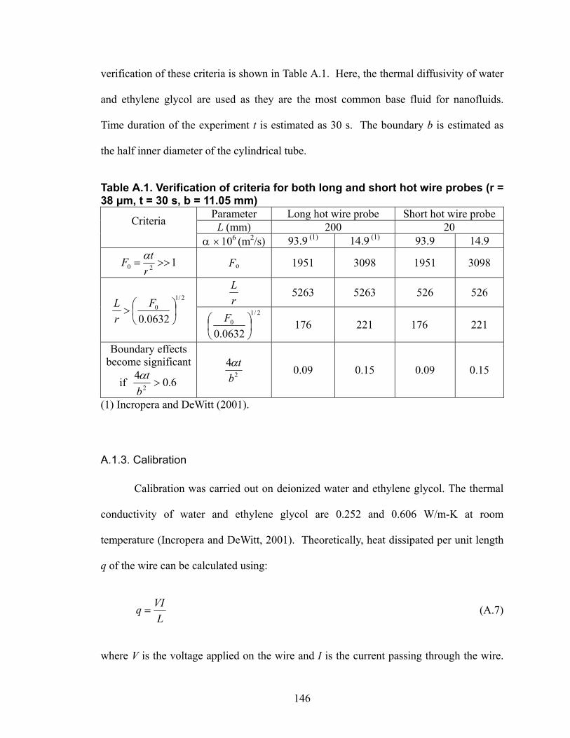
146

verification of these criteria is shown in Table A.1. Here, the thermal diffusivity of water

and ethylene glycol are used as they are the most common base fluid for nanofluids.

Time duration of the experiment t is estimated as 30 s. The boundary b is estimated as

the half inner diameter of the cylindrical tube.

Table A.1. Verification of criteria for both long and short hot wire probes (r = 38 μm, t = 30 s, b = 11.05 mm)

Parameter Long hot wire probe Short hot wire probe L (mm) 200 20 Criteria

α ×106 (m2/s) 93.9 (1) 14.9 (1) 93.9 14.9

120 >>=r

tF α Fo 1951 3098 1951 3098

rL 5263 5263 526 526 2/1

0

0632.0⎟⎠⎞

⎜⎝⎛>

FrL 2/1

0

0632.0⎟⎠⎞

⎜⎝⎛ F 176 221 176 221

Boundary effects become significant

if 6.042 >

btα

2

4b

tα 0.09 0.15 0.09 0.15

(1) Incropera and DeWitt (2001).

A.1.3. Calibration

Calibration was carried out on deionized water and ethylene glycol. The thermal

conductivity of water and ethylene glycol are 0.252 and 0.606 W/m-K at room

temperature (Incropera and DeWitt, 2001). Theoretically, heat dissipated per unit length

q of the wire can be calculated using:

LVIq = (A.7)

where V is the voltage applied on the wire and I is the current passing through the wire.

147

Since the output voltage of the DC power supply is known, both V and I can be

determined from Wheatstone bridge.

However, in reality, the platinum wire is connected to the circuit by connecting

wires, therefore, there is heat loss on these connecting wires and conjunctions. Especially

for short wire, this heat loss is even larger since its resistance is not that much larger than

the connecting wires. Also, there is uncertainty in the measurement of wire length.

Therefore, the heat dissipated per unit length q needs to be compensated when used in

Equation (A.5) to determine the thermal conductivity:

LVIq η= (A.8)

where η is determined by matching the measured thermal conductivity of water with the

literature value, which is 66% and 79% for short wire and long wire probe respectively.

To justify the accuracy of the apparatus, the thermal conductivity of ethylene glycol was

then measured, and it is in good agreement with literature value.

Sample data plot for ethylene glycol measured by both long and short wire probe

are shown in Figure A.3. Clearly, there exist linear relationship between temperature and

the logarithmic time within certain time interval. The departure from the linear line at the

end is because of the convection heat transfer effect. Also, it is obvious that the short

wire probe responds much faster than the long wire probe. A segment of data was chosen

such that the linearity is guaranteed within the selected region. This segment of data was

later used for linear fit in order to calculate the thermal conductivity. The corresponding

calculated thermal conductivity results for different selected time interval are also shown

in Figure A.3. It is clear that the later time interval gives a little higher value due to the

148

growing convection effect, but this difference is considerably small. To avoid both the

instability of the circuit right after switch-on and the severe convection effects, the time

interval of 3 to 6 (s) for long wire and 0.5 to 2 (s) for short wire are used for future

calculation. Thus, the measured thermal conductivity of ethylene glycol is 0.2519 and

0.2518 for long and short respectively. Obviously, both long and short wire probes can

give accurate results compared with the reference data — thermal conductivity of

ethylene glycol at room temperature is 0.252 W/m-K (Incropera and DeWitt, 2001).

A.2. Convection Heat Transfer Coefficient Measurements

A.2.1. Principle

For internal flow in a tube with constant surface heat flux q, as shown in Figure

A.4, the mean temperature of the fluid Tf (x) varies linearly with the axial distance from

the entrance x (Incropera and DeWitt, 2001):

( ) xQc

qSTxTp

inf ρ+= (A.9)

where Tin is the fluid temperature at the inlet, S is the surface perimeter, ρ, cp, Q are the

density, specific heat capacity, and flowrate of the fluid, respectively.

149

10-2 10-1 100 101 10226

28

30

32

34

36

38

40

42

Time, t (s)

Tem

pera

ture

( o C

)

Time interval for linear fit

(s)

Thermal conductivity

(W/K-m) 1-3 0.2505 1-6 0.2514 1-10 0.2518 3-6 0.2519 3-10 0.2523 6-10 0.2534

1-10 s

1-6 s

1-3 s

3-10 s

6-10 s 3-6 s

(a)

10-2 10-1 100 101 10240

45

50

55

60

65

70

75

80

85

Time, t (s)

Tem

pera

ture

( o C

)

0.5-3 s

0.5-2 s

0.5-1 s

1-3 s

2-3 s1-2 s

Time interval for linear fit

(s)

Thermal conductivity

(W/K-m) 0.5-1 0.2476 0.5-2 0.2505 0.5-3 0.2532 1-2 0.2518 1-3 0.2559 2-3 0.2628

(b)

Figure A.3. Sample thermal conductivity measurement data for ethylene glycol: (a) sample data measured by the long wire probe and (b) Sample data measured by the short wire probe

150

Figure A.4. Internal flow in a tube

In addition, the conservation of energy gives:

SLTTQc

q inoutp )( −=

ρ (A.10)

where Tout is the fluid temperature at the outlet, L is the length of the tube. The heat flux

q can be solved by measuring the fluid temperature at both inlet and outlet (Tin and Tout).

The local convection heat transfer coefficient is defined as:

( ) ( ) ( )xTxTqxh

fw −= (A.11)

where Tw(x) is the wall temperature at location x. The dimensionless convection heat

transfer coefficient, Nussult number, is defined as:

khDNu = (A.12)

where D is the tube diameter and k is the fluid thermal conductivity.

151

A.2.2. Experimental Setup

The schematic drawing and experimental setup of heat transfer coefficient

measurement design are shown in Figure A.5. The testing section consists of a stainless

steel tube with a diameter of 0.83 mm and a length of 304.8 mm which is considered as a

micro-size channel.

The flow loop is driven by a peristaltic pump (Newport FPU5-MT-N). A filter is

placed before the test section in order to avoid clogging. The test section consists of a

metallic tube, a heating element, and temperature sensors. The insulation for the two

setups are different because of the tubing size. The micro tube is placed inside a Teflon

pipe filled with fiberglass, while the regular tube is insulated by two layers of ceramic

insulation strips. Two T-type thermocouples are placed at the entrance and the exit of the

test section to measure the flow inlet and outlet temperature. Five T-type thermocouples

are evenly positioned along the tube to measure the wall temperature. The metallic tube

is heated by the DC power supply (BK Precision 1692, Test Equipment Depot) when the

fluid is passing through, and hence the forced convection heat transfer occurs. The outlet

fluid is then cooled by a flow-through chiller (VWR 1106), which is turned on and off

periodically by a temperature controller (Omega CN8592) in order to maintain the fluid

at the temperature before it enters the test section again. The wall temperatures and the

fluid temperatures at inlet and outlet are recorded after the system reaches a steady.

The volumetric flowrate was estimated by measuring the volume of fluid

transported per unit time. The heat loss δ can be estimated using:

VITTQc

Pq inoutptot )(

11−

−=−=ρ

δ (A.13)

152

where P is the input power of the DC power supply (P = VI), qtot represents the total heat

entering the flow, )( inoutptot TTQcq −= ρ , V and I are the output voltage and current of the

DC power supply, respectively. The heat loss in the experiments is about 5% in the

current setup.

Pump

DC Power Supply

Cooler

Thermocouple

Filter Valve

Flow

(a)

(b) Figure A.5. Convection heat transfer measurement apparatus: (a) convection heat transfer measurement schematic drawing and (b) experimental setup

A.2.3. Calibration Results

The calibration tests were conducted on pure water and the tested flow rate ranged

from 110 to 410 ml/min, which corresponds to Reynolds number of 3,600 to 14,000. The

Reynolds number is a dimensionless number, defined as

153

νUDRe = (A.14)

where U is the mean velocity of the fluid, D is the tube diameter, and νis the kinematic

viscosity. Since the critical Reynolds number corresponding to the onset of turbulence is

2,300 (Incropera and DeWitt, 2001), the tests for microchannel setup were conducted in

the turbulent regime.

Many correlations have been well-established for heat transfer flow such as

Hausen correlation and Shah correlation for laminar flow, Dittus-Boelter correlation and

Gnielinski correlation for turbulent flow (Incropera and DeWitt, 2001), but the

convective heat transfer behavior of flow in microchannels is still controversial. Morini

(2004) presented a detailed review of single-phase convective heat transfer in

microchannels and most of the experimental research work being reviewed does not

match well with the conventional theory. Some of those research works were conducted

in the circular cross-section microchannels (Bucci et al., 2003; Tso and Mahulikar, 2000;

Choi et al., 1991; Yu et al., 1995; Adams et al., 1998; Celata et al., 2000; Kandlikar et al.,

2001). Among these, only Bucci et al. (2003) reported that experimentally measured

Nusselt number agrees with the conventional theory. Tso and Mahulikar (2000) reported

that the measured Nusselt number is lower than the prediction of conventional theory.

All the other researches (Choi et al., 1991; Yu et al., 1995; Adams et al., 1998; Celata et

al., 2000; Kandlikar et al., 2001 ) showed that the Nusselt number is larger than that

predicted by conventional theory. Choi et al. (1991), Yu et al. (1995) and Adams et al.

(1998) also proposed correlations for convection heat transfer of flow in microchannels.

To verify our experimental setup and methodology, we will compare our experimental

154

results with their correlations as well as the conventional theory. Those convection heat

transfer correlations will be first introduced in the following:

Choi et al. (1991) studied the friction factors, inner wall surface roughness, and

convective heat transfer coefficients for flow of nitrogen gas in microtubes ranging from

3 – 81 μm in both laminar and turbulent regimes, and proposed correlations:

3/117.1 PrRe000972.0=Nu (Re < 2,000) (A.15)

3/196.16 PrRe1082.3 −×=Nu (2,500 < Re < 20,000) (A.16)

where Pr is Prandtl number, defined as: αυ

y,diffusivit thermal , viscositykinematicPr =

Yu et al. (1995) studied the fluid flow and heat transfer characteristics of dry

nitrogen gas and water in microtubes, with diameters of 19, 52, and 102 μm , for Re

ranging from 250 to over 20,000, and proposed a correlation:

2.02.1 PrRe007.0=Nu (6,000 < Re < 20,000) (A.17)

Adams et al. (1998) studied turbulent, single-phase forced convection of water in

circular microchannels with diameters of 0.76 and 1.09 mm, and modified the Gnielinski

correlation to accommodate the small diameters encountered in microchannels:

( )

⎟⎟⎠

⎞⎜⎜⎝

⎛⎟⎠⎞

⎜⎝⎛−×=

+=

−2

5

164.11Re106.7

1

DF

FNuNu Gn

(A.18)

for the range of conditions: 43.6Pr53.1 ≤≤ ; 000,23Re600,2 ≤≤ ; and

mm 09.1mm 102.0 ≤≤ D . where NuGn is given by Gnielinski equation (Incropera and

155

DeWitt, 2001), which is the well-known correlation for Nusselt number in turbulent

regime:

( )( )( ) ( )

( ) 2

3/22/1

64.1Reln790.0

1Pr8/7.121Pr1000Re8/

−−=

−+−

f

ffNuGn

(A.19)

for 6105Re2300 ×≤≤ and 200Pr5.0 ≤≤ .

0

100

200

300

400

500

600

700

800

900

0 2,500 5,000 7,500 10,000 12,500 15,000

Re

Nu

ExperimentYu et al. (1995)Choi et al. (1991)Adams et al. (1998)Gnielinski (Incropera and DeWitt, 2001)

Figure A.6. Microchannel setup calibration

The calibration results for microchannels are shown in Figure A.6. The measured

Nusselt number falls between the correlations in the literature. However, our

experimental results also indicted that the convection heat transfer coefficient in

microchannels is larger than that predicted by conventional theory (Gnielinski equation).

But they are very close to Adams correlation, this is most likely because the diameter of

156

our microchannel setup (0.83mm) is very close to that in Adams’ experiment (0.76 and

1.09 mm). Overall, the calibration results demonstrated that the current experimental

setup is capable to measure the convection heat transfer coefficient of fluids in the

microchannels.

157

Appendix B

Finite Difference Method Heat Transfer Modeling

B.1. Boundary Conditions

For the boundary condition within the grinding zone, as shown in Figure B-1, by

considering the heat conduction between the nodes, heat flux from the wheel-workpiece

interface, as well as the forced convection or convection with phase change within the

grinding zone, the energy conservation gives:

( )[ ]amcontactopmmmmmm TtTAGtTVcAqqqq −+

∂∂

=+++ →→+→− 1,)1,()2,()1,()1,1()1,()1,1( " ρ (B.1)

where ρ, Cp are the density and the specific heat capacity of workpiece, Ta the fluid (or

ambient) temperature; 1zxVo ••= ΔΔ ; 1xA •= Δ ; and Gcontact is the combined heat

transfer coefficient, defined as:

1

21

−

⎟⎟⎠

⎞⎜⎜⎝

⎛ Δ+=

kz

hG

contactcontact

(B.2)

where hcontact is the convection heat transfer coefficient within the contact zone, and k is

the thermal conductivity of the workpiece. The heat flux terms can be expressed as:

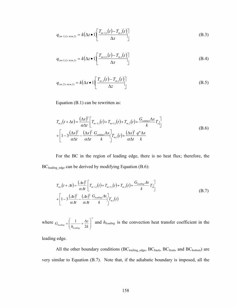
158

( ) ( ) ( )⎥⎦

⎤⎢⎣

⎡Δ

−•Δ= −

→− xtTtT

zkq mmmm

1,1,1)1,()1,1( 1 (B.3)

( ) ( ) ( )⎥⎦

⎤⎢⎣

⎡Δ

−•Δ= +

→+ xtTtT

zkq mmmm

1,1,1)1,()1,1( 1 (B.4)

( ) ( ) ( )⎥⎦

⎤⎢⎣

⎡Δ−

•Δ=→ ztTtT

xkq mmmm

1,2,)1,()2,( 1 (B.5)

Equation (B.1) can be rewritten as:

( ) ( ) ( ) ( ) ( )

( ) ( ) ( ) ( )k

xqt

xtTk

xGt

xt

x

Tk

xGtTtTtTt

xttT

mcontact

acontact

mmmm

ΔΔ

Δ+⎥

⎦

⎤⎢⎣

⎡ ΔΔ

Δ−

ΔΔ

−+

⎥⎦⎤

⎢⎣⎡ Δ

+++Δ

Δ=Δ+ +−

"312

1,

22

2,1,11,1

2

1,

ααα

α (B.6)

For the BC in the region of leading edge, there is no heat flux; therefore, the

BCleading_edge can be derived by modifying Equation (B.6):

( ) ( ) ( ) ( ) ( )

( ) ( ) ( )tTk

xGt

xt

x

Tk

xGtTtTtT

txttT

,mleading

aleading

,m,m,m,m

1

22

21111

2

1

31 ⎥⎦

⎤⎢⎣

⎡−−+

⎥⎦

⎤⎢⎣

⎡+++=+ +−

ΔΔα

ΔΔα

Δ

ΔΔα

ΔΔ (B.7)

where 1

21

−

⎟⎟⎠

⎞⎜⎜⎝

⎛ Δ+=

kz

hG

leadingleading

and hleading is the convection heat transfer coefficient in the

leading edge.

All the other boundary conditions (BCtrailing_edge, BCback, BCfront, and BCbottom) are

very similar to Equation (B.7). Note that, if the adiabatic boundary is imposed, all the

159

BCs will still hold by simply setting the convection heat transfer coefficient (hcontact,

hleading, htrailing, hfront, or hback) to zero.

Figure B.1. BC within the contact zone

B.2. Surface Temperature

As seen in Figure B.2, the energy conversation at the surface (within the contact

zone) gives:

( )[ ]a,mcontact),m(surface TtTsAhqA"q −+= → 11 (B.8)

( ) ( ) ( ) ( ) ( ) ( )[ ]as,mcontact

,ms,m TtTxh

/ztTtT

xkx"q −•+⎥⎦

⎤⎢⎣

⎡ −•=• 1

11 12

11 ΔΔ

ΔΔ (B.9)

( ) ( )( )kzh

kzThtTkzqtT

contact

acontactmsm /2

/2/" 1,1, Δ+

Δ++Δ= (B.10)

Similarly, the surface temperature in the region of leading and trailing edges can

be expressed as following, respectively.

160

( ) ( )( )kzh

kzThtTtT

leading

aleadingmsm /2

/2 1,1, Δ+

Δ+= (B.11)

( ) ( )( )kzh

kzThtTtT

trailing

aatrailingmsm /2

/2 1,1, Δ+

Δ+= (B.12)

Figure B.2. Interpretation of the surface temperature (contact zone)

161

BIBLIOGRAPHY

162

Bibliography

Adams, T.M., Abdel-Khalik S.I., Jeter S.M., and Qureshi Z.H., 1998, “An experimental investigation of single-phase forced convection in microchannels,” International Journal of Heat and Mass Transfer, vol. 41, pp. 851–857.

Assael, M.J., Chen, C.F., Metaxa, I., Wakeham, and W.A., 2004, “Thermal conductivity of suspensions of carbon nanotubes in water,” International Journal of Thermophysics, vol. 25, no. 4, pp. 971-985.

Autret, R., and Liang, S.Y., 2003, “Minimum quantity lubrication in finish hard turning,” HNICEM ’03.

Baheti, U., Guo, C., and Malkin, S., 1998, “Environmentally conscious cooling and lubrication for grinding,” Proceedings of the International Seminar on Improving Machine Tool Performance, vol. 2, pp. 643-654.

Batty, W.J., O’Callaghan, P.W., and Probert, S.D., 1984, “Assessment of the thermal-probe technique for rapid, accurate measurements of effective thermal conductivities,” Applied Energy, vol. 16, pp. 83-113.

Baheti, U., Guo, C., and Malkin, S., 1998, “Environmentally conscious cooling and lubrication for grinding,” Proceedings of the International Seminar on Improving Machine Tool Performance, vol. 2, pp. 643-654.

Batako, A.D., Rowe, W.B., and Morgan, M.N., 2005, “Temperature measurement in high efficiency deep grinding,” Int. J. Machine Tools Manuf., vol. 45, pp.1231-1245.

Biermann, D. and Schneider, M., 1997, “Modeling and simulation of workpiece temperature in grinding by finite element analysis,” Machining Science and Technology, vol. 1, no. 2, pp. 173-183.

Blackwell, J.H., 1954. “A transient-flow method for determination of thermal constants of insulating materials in bulk,” J. Appl. Phys., vol. 25, no. 2, pp.137–144.

163

Braga, D.U., Diniz, A.E., Miranda, G.W.A., and Coppini, N.L., 2002, “Using a minimum quantity of lubricant (MQL) and a diamond coated tool in the drilling of aluminum-silicon alloys,” Journal of Materials Processing Technology, vol. 122, no. 1, pp. 127-138.

Brinksmeier, E., Brockhoff, T., and Walter, A., 1997, “Minimalmengenkühlschmierung und Trockenbearbeitung beim Schleifen,” Haerterei-Technische Mitteilungen, vol. 52, pp. 166-170.

Bucci, A., Celata, G.P., Cumo, M., Serra, E., and Zummo, G., 2003, “Fluid flow and single-phase flow heat transfer of water in capillary tubes,” Proceedings of the Int. Conference on Minichannels and Microchannels, Rochester, USA, paper ICMM-1037.

Carslaw, H.S., and Jaeger, J.C., 1959, Conduction of heat in solids, 2nd Edition, Clarendon Press., Oxford, pp. 169 -170.

Castro, C.A.N, Calado, J.C.G, Wakeham, W.A, and Dix, M., 1976, “An apparatus to measure the thermal conductivity of liquids,” J Phys E Sci Instrum, vol. 9, pp. 1073-1080.

Celata, G.P., Cumo, M., Guglielmi, M., and Zummo G., 2000, “Experimental investigation of hydraulic and single phase heat transfer in 0.130 mm capillary tube,” Proceedings of International Conference on Heat Transfer and Transport Phenomena in Microscale,” Begell House, New York, USA, pp. 108–113.

Che, J.W., Cagin, T., Goddard, W.A., 2000, “Thermal conductivity of carbon nanotubes,” Nanotechnology, vol. 11, pp. 65-69.

Chen, Z., Yamaguchi, H., and Liang, S.Y., 2002a, “Predictive modeling of cutting fluid aerosol in grinding process,” Transactions of the North American Manufacturing Research Institution, Society of Manufacturing Engineers, pp. 277-285.

Chen, Z., Liang S.Y., and Yamaguchi, H., 2002b, “Predictive modeling of cutting fluid aerosol generation in cylindrical grinding,” Society of Manufacturing Engineers, vol. 160, pp. 1-8.

Choi, S.B., Barron, R.F., and Warrington, R.O., 1991, “Fluid flow and heat transfer in microtubes,” Micromechanical Sensors, Actuators and Systems, ASME DSC, vol. 32, Atlanta, GA, pp. 123–134.

Choi, S.U.S., 1995, “Enhancing thermal conductivity of fluids with nanoparticles,” Proceedings of the 1995 ASME International Mechanical Engineering Congress

164

and Exposition, San Francisco, CA, USA.

Choi, S.U.S., Li, S., Yu, W., and Thompson, L.J., 2001a, “Anomalously increased effective thermal conductivities of ethylene glycol-based nanofluids containing copper nanoparticles,” Applied Physics Letters, vol. 78, no. 6, pp. 718-720.

Choi, S.U.S., Zhang, Z.G., Yu, W., Lockwood, F.E, and Grulke, E.A., 2001b, “Anomalous thermal conductivity enhancement in nanotube suspensions,” Applied Physics Letters, vol. 79, pp. 2252-2254.

Choi, S.U.S., and Eastman, J.A., 2001, “Enhanced heat transfer using nanofluids,” US Patent Number 6,221,275.

Curry, A.C., Shih, A.J., Scattergood, R.O., Kong, J., and McSpadden, S.B., 2003, “Grinding temperature measurements in MgO PSZ using infrared spectrometry,” J. Am. Ceram. Soc., vol. 86, pp. 333-341.

Das, S.K., Putra, N., Thiesen, R., and Roetzel, W., 2003, “Temperature dependence of thermal conductivity enhancement for nanofluids,” Journal of Heat Transfer, vol. 125, no. 4, pp. 567-574.

Davim, J.P., Sreejith, P.S., Gomes, R., and Peixoto, C., 2006, “Experimental studies on drilling of aluminum (AA1050) under dry, minimum quantity of lubricant, and flood-lubricated conditions,” J. Engineering Manufacture, vol. 220, pp. 1605-1611.

Davim, J.P., Sreejith, P.S. and Silva, J., 2007, “Turning of brasses using minimum quantity of lubricant and flooded lubricant conditions,” Materials and Manufacturing Processes, vol. 22, pp. 45-50.

DeGroot, J.J, J. Kestin, and H. Sookiazian, 1974, “Instrument to measure the thermal conductivity of gases,” Physica, vol. 75, pp. 454-482.

Demetriou, M.D., and Lavine, A.S., 2000, “Thermal aspects of grinding, the case of upgrinding,” J. Manuf. Sci. Eng., vol. 122, pp. 605-611.

DesRuisseaux, N.R., and Zerkle, R.D., 1970, “Thermal analysis of the grinding process,” ASME J. Eng. Ind., vol. 92, pp. 428-434.

Dhar, N.R., Islam, M.W., Islam, S., and Mithu, M.A.H., 2006, “The influence of minimum quantity of lubrication (MQL) on cutting temperature, chip and dimensional accuracy in turning AISI-1040 steel,” Journal of Materials Processing Technology, vol. 171, pp. 93-99.

165

Dhar, N.R., Ahmed, M.T., and Islam, S., 2007, “An experimental investigation on effect of minimum quantity lubrication in machining AISI 1040 steel,” International Journal of Machine Tools and Manufacture, vol. 47, no. 5, pp. 748-753.

Eastman, J.A., Choi, S.U.S., Li S., Thompson L.J., and Lee S., 1997, “Enhanced thermal conductivity through development of nanofluids,” Materials II, ed. S Komarnenl, JC Parker, HJ Wollenberger, pp. 3. Pittsburgh: Materials Research Society.

Eastman, JA, Choi, S.U.S., Li, S., Yu, W., and Thompson, L.J., 2001, “Anomalously increased effective thermal conductivity of ethylene glycol-based nanofluids containing copper nanoparticles,” Applied Physics Letters, vol. 78, no. 6, pp. 718-720.

Eastman, J.A., Phillpot, S.R., Choi, S.U.S., Keblinski, P., 2004, “Thermal transport in nanofluids,” Annual Review of Materials Research, vol. 34, pp. 219-246.

Filipovic, A., and Stephenson, D.A., 2006, “Minimum quantity lubrication applications in automotive power-train machining,” Machining Science and Technology, vol. no. 10, pp. 3-22.

Florescu, D.I., Mourokh, L.G., Pollak, F.H., Look, D.C. , Cantwell, G., Li, X., 2002, “High spatial resolution thermal conductivity of bulk ZnO,” Journal of Applied Physics, vol. 91, no.2, pp. 890-892.

Fuh, K.H., and Huang, J.S., 1994, “Thermal analysis of creep-feed grinding,” J. Materials Proc. Technology, vol. 43, pp. 109-124.

Furness, R., Stoll, A., Nordstrom, G.. Martini, G., Johnson, J., Loch, T., and Klosinski, R., 2006, “Minimum Quantity Lubrication (MQL) machining for complex powertrain components,” Proceedings of the International Conference on Manufacturing Science and Engineering.

Guo, C., and Malkin, S., 1992, “Heat transfer in grinding,” J. Materials Proc. Manuf. Sci., vol. 1, pp. 16-27.

Guo, C., Wu, Y., Varghese, V., and Malkin, S., 1999, ‘‘Temperatures and energy partition for grinding with vitrified CBN wheels,’’ CIRP Annals, vol. 48, pp. 247-250.

Guo, C., and Malkin, S., 1995a, “Analysis of energy partition in grinding,” Journal of Engineering for Industry, vol.117, pp. 55–61.

Guo, C. and Malkin, S., 1995b, “Analysis of transient temperatures in grinding,” Journal of Engineering for Industry, vol. 117, pp. 571-577.

166

Guo, C., and Malkin, S., 1996a, “Inverse heat transfer analysis of grinding, part 1: Methods,” Journal of Engineering for Industry, vol. 118, no. 1, pp. 137-142.

Guo, C., and Malkin, S., 1996b, “Inverse heat transfer analysis of grinding, part 2: Applications,” Journal of Engineering for Industry, vol. 118, no. 1, pp. 143-149.

Hafenbraedl, D., and Malkin, S., 2000, “Environmentally-conscious minimum quantity lubrication (MQL) for internal cylindrical grinding,” Transactions of NAMRI/SME, vol. 28, pp. 149-154.

Hahn, R.S., 1956, “The relation between grinding conditions and thermal damage in the workpiece ,” Transactions of the ASME, vol. 78, pp. 807-812.

Hahn. R.S., 1962, “On the nature of the grinding process,” Proceedings of the 3rd Machine Tool Design and Research Conference, pp. 129-154.

Hahn R S., 1966, “On the mechanics of the grinding process under plunge cut conditions,” Journal of Engineering for Industry, vol. 88, pp. 72-80.

Hamilton, R.L. and Crosser, O. K., 1962, “Thermal conductivity of heterogeneous two-component systems,” I&EC Fundamentals, vol. 1, no. 3, pp. 187-191.

Heinemann, R., Hinduja, S., Barrow, G., and Petuelli, G., 2006, “Effect of MQL on the tool life of small twist drills in deep-hole drilling,” International Journal of Machine Tools and Manufacture, vol. 46, pp. 1-6.

Hong, K.K. and Lo, C.Y., 2000, “Inverse analysis for the heat conduction during a grinding process,” Journal of Materials Processing Technology, vol. 105, no. 1, pp. 87-94.

Hong, T.K., Yang, H.S., and Choi, C.J., 2005, “Study of the enhanced thermal conductivity of Fe nanofluids,” J. Appl. Phys., vol. 97, 64311.

Hoshi, M., Omotani, T., and Nagashima, A., 1981, “Transient method to measure the thermal conductivity of high-temperature melts using a liquid-metal probe,” Review of Scientific Instruments, vol. 52, no. 5, pp. 755-758.

Huang, H., and Xu, X.P., 2004, “Interfacial interactions between diamond disk and granite during vertical spindle grinding,” Wear, vol. 256, pp. 623-629.

Hwang, J., Kompella, Sridhar, S., Chandrasekar, S., and Farris, T.N., 2003, “Measurement of temperature field in surface grinding using Infra-Red (IR) imaging system,” J. Tribology, vol. 125, pp. 377-383.

167

Incropera, F.P. and DeWitt, D.P., 2001, Fundamentals of Heat and Mass Transfer, 5th Edition, Wiley.

Itoigawa, F., Childs, T.H.C., Nakamura, T., and Belluco, W., 2006, “Effects and mechanisms in minimal quantity lubrication machining of an aluminum alloy," Wear, vol. 260, no. 3, pp. 339-344.

Jaeger, J.C., 1942, “Moving sources of heat and the temperature at sliding contacts,” Journal of the Royal Society of New South Wales, vol. 76, pp. 203–224.

Jang S.P. and Choi S.U.S., 2004, “Role of Brownian motion in the enhanced thermal conductivity of nanofluid,” Appl. Phys. Lett., vol. 84, no. 21, pp. 4316–4318.

Jeffrey, D.J., 1973, “Conduction through a random suspension of spheres,” Proceedings of the Royal Society of London, Series A, vol. 335, no. 1602, pp. 355–367.

Jen, T.C. and Lavine, A.S., 1995, “A variable heat flux model of heat transfer in grinding: model development,” Journal of Heat Transfer, vol. 117, no. 2, pp. 473-478.

Ju, Y., Farris, T.N., and Chandrasekar, S., 1998, “Theoretical analysis of heat partition and temperatures in grinding,” Journal of Tribology, vol. 120, no. 4, pp. 789-794.

Kamata, Y., and Obikawa, T., 2007, “High speed MQL finish-turning of Inconel 718 with different coated tools,” Journal of Materials Prorcessing Technology, vol. 192, pp. 281-286.

Kandlikar, S.G., Joshi, S., and Tian, S., 2001, “Effect of channel roughness on heat transfer and fluid flow characteristics at low Reynolds numbers in small diameter tubes,” Proc. of 35th National Heat Transfer Conference, Anaheim CA, USA, paper 12134.

Keblinski, P., Phillpot, S.R., Choi, S.U.S., and Eastman J.A., 2002, “Mechanisms of heat flow in suspensions of nano-sized particles (nanofluids),” International Journal of Heat and Mass Transfer, vol. 45, no. 4, pp. 855-863.

Kim, H.J., Kim, N.K., and Kwak, J.S., 2006, “Heat flux distribution model by sequential algorithm of inverse heat transfer for determining workpiece temperature in creep feed grinding,” International Journal of Machine Tools and Manufacture, vol. 46, no. 15, pp. 2086-2093.

Klocke, F., and Eisenblatter, G., 1997, “Dry cutting,” Annals of the CIRP, vol. 46, pp. 519-526.

168

Kobayashi, S., Ohgoe, Y., Ozeki, K., Sato, K., Sumiya, T., Hirakuri, K.K., and Aoki, H., 2005, “Diamond-like carbon coatings on orthodontic archwire,” Diamond and Related Materials, vol. 14, pp. 1094-1097.

Kohli, S. P., Guo, C., and Malkin, S., 1995, ‘‘Energy partition for grinding with aluminum oxide and CBN abrasive wheels,’’ Journal of Engineering for Industry, vol. 117, pp. 160–168.

Komanduri, R., and Reed, W.R., 1980, “New technique of dressing and conditioning resin bonded superabrasive grinding wheels,” Annals of the CIRP, vol. 29, no. 1, pp. 239-243.

Lavine, A.S., 1988, “A simple model for convective cooling during the grinding process,” Journal of Engineering for Industry, vol. 110, pp. 1-6.

Lavine, A.S., Malkin, S., and Jen, T., 1989, ‘‘Thermal Aspects of Grinding with CBN,” CIRP Ann., vol. 38, pp. 557–560.

Lee, S., Choi, S.U.S., Li, S., and Eastman, J.A., 1999, “Measuring thermal conductivity of fluids containing oxide nanoparticles,” ASME Journal of Heat Transfer, vol. 121, no. 2, pp. 280-289.

Lefebvre, A., Vieville, P., Lipinski, P., and Lescalier, C., 2006, “Numerical analysis of grinding temperature measurement by the foil/workpiece thermocouple method,” International Journal of Machine Tools and Manufacture, vol. 46, no. 14, pp. 1716-1726.

Liao, Y.S., Luo, S.Y. and Yang, T.H., 2000, “Thermal model of the wet grinding process,” Journal of Materials Processing Technology, vol. 101, no. 1, pp. 137-145.

Liao, Y.S., and Lin, H.M., 2007, “Mechanism of minimum quantity lubrication in high-speed milling of hardened steel,” International Journal of Machine Tools and Manufacture, vol. 47, pp. 1660-1666.

Littman, W.E., and Wulff, J., 1995, “The influence of the grinding process on structure of hardened steels,” Trans. Am. Soc. Metals, vol. 47, pp. 692.

Lockwood, F.E., Zhang, Z.G., Forbus, T.R., Choi, S.U.S., Yang, Y., and Grulke, E.A., 2005, “The current development on nanofluid research,” SAE 2005 World Congress & Exhibition, Detroit, MI, USA, Session: Military Vehicle Fuels, Lubes and Water.

Lopez de Lacalle, L.N., Angulo, C., Lamikiz, A., and Sanchez, J.A., 2006, “Experimental

169

and numerical investigation of the effect of spray cutting fluids in high speed milling,” Journal of Materials Processing Technology, vol. 172, pp. 11-15.

Lowenthal, G.C. and Harper, A.F.A., 1960, “Resistance-temperature relationship of platinum at low temperatures and its influence on precision thermometry,” J. Appl. Phys., vol. 11, pp. 205-208.

Machado, A. R., and Wallbank, J., 1997, “Effect of extremely low lubricant volumes inachining,” Wear, vol. 210, pp. 76-82.

Mahdi, M. and Zhang L., 1995, “The finite element thermal analysis of grinding processes by ADINA,” Computer and Structure, vol. 56, pp. 313–320.

Maksoud, T.M.A., 2005, “Heat transfer model for creep-feed grinding,” Journal of Materials Processing Technology, vol. 168, no. 3, pp. 448-463.

Malkin, S., and Anderson, R.B., 1974, “Thermal aspects of grinding. Part 1 - Energy Partition,” ASME J. Eng. Ind., vol. 96, pp. 1177-1183.

Malkin S., 1984, “Grinding of metals: theory and application,” Journal of Applied Metalworking, America Society for Metals, vol. 3, no. 2, pp. 95-109.

Malkin, S., 1989, Grinding Technology: Theory and Applications of Machining with Abrasives, Ellis Horwood Ltd, Chichester, and John Wiley & Sons, New York.

Malshe, A.P., and Verma, A., 2006, “Nanoparticle compositions and methods for making and using the same,” International Application No. PCT/US07/60506.

Mamalis, A.G., Kundrak, J., Manolakos, D.E., Gyani, K., and Markopoulos, A., 2003, “Thermal modelling of surface grinding using implicit finite element techniques,” International Journal of Advanced Manufacturing Technology, vol. 21, no. 12, pp. 929-934.

Masuda, H., Ebata, A., Teramae, K., and Hishinuma, N., 1993, “Alteration of thermal conductivity and viscosity of liquid by dispersing ultra-fine particles (dispersion of γ -Al2O3, SiO2 and TiO2 ultra-fine particles),” Netsu Bussei, vol.4, pp. 227-233.

Maxwell, J.C., 1904, A Treatise on Electricity and Magnetism, 2nd ed. Oxford University Press, Cambridge, U.K., 1904, pp. 435–441.

Morini, G.L., 2004, "Single-phase convective heat transfer in microchannels: A Review of Experimental Results," Int. J. Therm. Sci., vol. 43, pp. 631–651.

170

Murshed, S.M.S., Leong, K.C., and Yang, C., 2005, “Enhanced thermal conductivity of TiO2 - water based nanofluids,” International Journal of Thermal Sciences, vol. 44, pp. 367-373.

Nagasaka, Y, and Nagashima, A., 1981, “Absolute measurement of the thermal conductivity of electrically conducting liquids by transient hot-wire method”, J Phys E Sci Instrum, 1981, vol. 14, pp. 1435-1440.

Nouari, M., List, G., Girot, F., and Coupard, D., 2003, “Experimental analysis and optimisation of tool wear in dry machining of aluminium alloys,” Wear, vol. 255, pp. 1359-1368.

Outwater, J.O., and Shaw, M.C., 1952, “Surface temperatures in grinding,” Trans. ASME, vol. 74, pp. 73-86.

Ozisik, M.N., 1994, Finite Difference Methods in Heat Transfer, CRC Press.

Pak, B.C., and Cho, Y.I., 1998, ‘‘Hydrodynamic and heat transfer study of dispersed fluids with submicron metallic oxide particles,’’ Exp. Heat Transfer, vol. 11, pp. 151-170.

Patel, H.E., Das, S.K., Sundararajan, T., Nair, A.S., George, B., and Pradeep, T., 2003, “Thermal conductivities of naked and monolayer protected metal nano-particle based nano-fluids: manifestation of anomalous enhancement and chemical effects,” Applied Physics Letters, vol. 83, no. 14, pp. 2931-2933.

Rahman, M., Senthil Kumar, A., and Salam, M. U., 2001, “Evaluation of minimal quantities of lubricant in end milling,” International Journal of Advanced Manufacturing Technology, vol. 18, no. 4, pp. 235-241.

Rahman, M., Kumar, A.S., and Salam, M.U., 2002, “Experimental evaluation on the effect of minimal quantities of lubricant in milling,” International Journal of Machine Tools and Manufacture, vol. 42, no. 5, pp. 539-547.

Reddy, N.S.K., and Rao, P.V., 2006, “Selection of an optimal parametric combination for achieving a better surface finish in dry milling using genetic algorithms,” International Journal of Advanced Manufacturing Technology, vol. 28, pp. 463-473.

Rowe, W.B., Pettit, J.A., Boyle, A., and Moruzzi, J.L., 1988, “Avoidance of thermal damage in grinding,” Annals of CIRP, vol. 37, pp. 327-330.

Rowe, W. B., Black, S.C.E., Mills, B., Qi, H. S., Morgan, M.N, 1995, “Experimental

171

investigation of heat transfer in grinding,” Annals of the CIRP, vol. 44, pp. 329-332.

Rowe, W.B., Black, S.C.E., and Mills, B., 1996, “Temperature control in CBN grinding,” Int. J. Advanced Manuf. Technology, vol. 12, pp. 387-392.

Sakagami, T., Madhavan, V., Harish, G., Krishnamurthy, K., Ju, Y., Farris, T.N. and Chandrasekar, S., 1990, “Full-field IR measurement of subsurface grinding temperatures,” Proc. of SPIE, vol. 3361, pp. 234-245.

Shaw M.C., 1990, “A simplified approach to workpiece temperature in fine grinding,” CIRP. Annals, vol. 39, pp. 345-347.

Shen, C.H., 1996, “The importance of diamond coated tools for agile manufacturing and dry machining,” Surface and Coating Technology, vol. 86-87, pp. 672-677.

Shen, B, Shih, A.J., and Tung, S.C., 2008a, “Application of nanofluids in minimum quantity lubrication grinding,” accepted for STLE (Society of Tribologists and Lubrication Engineers) Tribology Transactions.

Shen, B., Malshe, A.P., Kalita, P., and Shih, A.J., 2008b, “Performance and behavior of novel MoS2 nanoparticles based grinding fluids in minimum quantity lubrication grinding” accepted for NAMRI/SME, vol 36.

Shen, B., Xiao, G., Guo, C., Malkin, S., and Shih, A.J., 2009, “Thermocouple fixating method for grinding temperature measurement,” submitted to ASME Journal of Manufacturing Science and Engineering.

Shen, B., and Shih, A.J., 2009, “Minimum quantity lubrication (MQL) grinding using vitrified CBN wheels,” submitted to NAMRI/SME, vol. 37.

Shih, A.J., Curry A.C., Scattergood, R.O., Yonushonis, T.M., Gust, D.J., Grant, M.B., McSpadden, S.B., and Watkins, Y., 2003, “Cost-effective grinding of zirconia using the dense vitreous bond silicon carbide wheel,” Journal of Manufacturing Science and Engineering, vol. 125, pp. 297-303.

Silva, L.R., Bianchi, E.C., Catai, R.E., Fusse, R.Y., and Franca, T.V., 2005, “Study on the behavior of the minimum quantity lubricant - MQL technique under different lubricating and cooling conditions when grinding ABNT 4340 steel,” Journal of the Brazilian Society of Mechanical Sciences and Engineering, vol. 27, no. 2, pp. 192-199.

Su, Y.L., Liu, T.H., Su, C.T., Yao, S.H., Kao, W.H., and Cheng, K.W., 2006, “Wear of

172

CrC-coated carbide tools in dry machining,” Journal of Materials Processing Technology, vol. 171, pp. 108-117.

Sun, J., Wong, Y.S., Rahman, M., Wang, Z.G., Neo, K.S., Tan, C.H., and Onozuka, H., 2006, “Effects of coolant supply methods and cutting conditions on tool life in end milling titanium alloy,” Machining Science and Technology, vol. 10, pp. 355-370.

Takazawa, K., 1966, “Effects of grinding variables on the surface of hardened steel,” Bull. Japan Soc. Prec. Eng., vol. 2, pp. 14-21.

Takazawa, K., 1972, “Thermal aspects of the grinding operation,” Industrial Diamond Review, pp. 143-149.

Tso, C.P., and Mahulikar, S.P., 2000, “Experimental verification of the role of Brinkman number in microchannels using local parameters,” Internat. J. Heat Mass Transfer, vol. 4, pp. 1837–1849.

Ueda, K.Y., and Sugita, T., 1992, “Measurement of grinding temperature of ceramics using infrared radiation pyrometer with optical fiber,” ASME J. Eng. Ind., vol. 114, pp. 317-21.

Ueda, T., 1986, “Measurement of grinding temperature using infrared radiation pyrometer with optical fiber,” ASME J. Eng. Ind., vol. 108, pp. 241-247.

Upadhyaya, R.P., and Malkin, S., 2004, “Thermal aspects of grinding with electroplated CBN wheels,” ASME J. Manuf. Sci. Eng., vol. 126, pp. 107-114.

Varghese, V., Guo, C., Malkin, S., and Xiao, G., 2000, ‘‘Energy partition for grinding of nodular cast iron with vitrified CBN wheels,’’ Mach. Sci. Technol., vol. 4, pp. 197-208.

Verma, A., Malshe, A.P., Brown, W., Jiang, W., Adhvaryu, A., and McCluskey, P., 2006, “Exploring mechanical synthesis of inorganic nanoparticles of MoS2 lubricant and its composite with organic medium for advanced manufacturing,” 4th International Symposium on Nanomanufacturing (ISNM).

Verma, A., Jiang, W., Abu-Safe, H.H., and Malshe, A.P., 2007, “Tribological behavior of the deagglomerated active inorganic nanoparticles for advanced lubrication,” accepted to Tribology Transactions.

Vos, B.H., 1955, “Measurements of thermal conductivity by non-steady-state method,” Appl. Sci. Res., Sec. A, vol. 5, pp. 425 - 438.

173

Wagener, M., Murty, B.S., Gunther, B., 1997, “Preparation of metal nanosuspensions by high-pressure DC-sputtering on running liquids,” Nanocrystalline and Nanocomposite Materials II, ed. S Komarnenl, JC Parker, HJ Wollenberger, Pittsburgh: Materials Research Society., pp. 149.

Wagener, M., Gunther, B., 1999, “Sputtering in liquids: a versatile process for the production of magnetic suspensions,” J. Magn. Magn. Mater., vol., 201, no. 4.

Wakabayashi, T., Sato, H., and Inasaki, I., 1998, “Turning using extremely small amounts of cutting fluids,” JSME International Journal, vol. 41, pp. 143-148.

Wang, X., Xu, X., and Choi, S.U.S., 1999, “Thermal conductivity of nanoparticle-fluid mixture,” J. Thermophys. Heat Transfer, vol. 13, no. 4, pp. 474–480.

Wang, C.C., and Chen, C.K., 2002, “Three-dimensional inverse heat transfer analysis during the grinding process,” Journal of Mechanical Engineering Science, vol. 216, pp. 199–214.

Wang, L., Qin, Y., Liu, Z.C., Ge, P.Q., and Gao, W., 2003, “Computer simulation of a workpiece temperature field during the grinding process,” Journal of Engineering Manufacture, vol. 217, no. 7, pp. 953-959.

Wen, D., and Ding, Y., 2004a, “Experimental investigation into convective heat transfer of nanofluids at the entrance region under laminar flow conditions, International Journal of Heat and Mass Transfer, vol. 47, no. 24, pp. 5181-5188.

Wen, D., and Ding, Y., 2004b, “Effective thermal conductivity of aqueous suspensions of carbon nanotubes (carbon nanotube nanofluids),” Journal of Thermophysics and Heat Transfer, vol. 18, no. 4, pp. 481-485.

White, S., 2006, GM Summer intern report.

Wu, J.H., Phillips, B.S., Jiang, W., Sanders, J.H., Zabinski, J.S., and Malshe, A.P., 2006, “Bio-inspired surface engineering and tribology of MoS2 overcoated CBN-TiN composite coating.” Wear, vol. 261, pp. 592-599.

Xie, H., Wang, J., Xi, T., Liu, Y., Ai, F. and Wu, Q., 2002a, “Thermal conductivity enhancement of suspensions containing nanosized alumina particles,” J. Appl. Phys., vol. 91, pp. 4568-4572.

Xie, H., Wang, J., Xi, T., and Liu, Y., 2002b, “Thermal conductivity of suspensions containing nanosized SiC particles,” Int J Thermophys, vol. 23, no. 2, pp. 571-580.

174

Xie, H., Lee, H., You, W., and Choi, M., 2003, “Nanofluids containing multiwalled carbon nanotubes and their enhanced thermal properties,” Journal of Applied Physics, vol. 94, no. 8, pp. 4967–4971

Xu, T., Zhang, J., and Xu, K., 1996, “The ball-bearing effect of diamond nanoparticles as an oil additive,” Applied Physics, vol. 29, pp. 2932-2937.

Xu, X.P., and Malkin, S., 2001, “Comparison of methods to measure grinding temperatures,” ASME J. Manuf. Sci. Eng., vol. 123, pp. 191-195.

Xu, X., Yu, Y., and Huang, H., 2003, “Mechanisms of abrasive wear in the grinding of titanium (TC4) and nickel (K417) alloys,” Wear, vol. 255, pp. 1421-1426.

Xuan, Y., and Roetzel, W., 2000, “Conceptions for heat transfer correlation of nanofluids,” International Journal of Heat and Mass Transfer, vol. 43, no. 19, pp. 3701-3707.

Xuan, Y., and Li, Q., 2000, “Heat transfer enhancement of nanofluids,” Int. J. Heat & Flow, vol. 21, no. 1, pp. 58-64.

Xuan, Y., and Li, Q., 2003, “Investigation on convective heat transfer and flow features of nanofluids,” Journal of Heat Transfer, vol. 125, no.1, pp. 151-155.

Yang, Y., Zhong Z.G., Grulke E.A., Anderson W.B. and Wu G., 2005, “Heat transfer properties of nanoparticle-in-fluid dispersion (nanofluids) in laminar flow,” Int. J. Heat Mass Transfer, vol. 48. pp. 1107–1116.

Yatsuya, S., Tsukasaki, Y., Mihama, K., Uyeda, R., 1978, “Preparation of extremely fine particles by vacuum evaporation onto a running oil substrate,” J. Cryst. Growth, vol. 45, pp. 490-494.

Yu, D., Warrington R.O., Barron, R., and Ameel, T., 1995, “An experimental and theoretical investigation of fluid flow and heat transfer in microtubes,” Proceedings of ASME/JSME Thermal Engineering Joint Conf., Maui, HI, pp. 523–530.

Zhu, H.T., Lin, Y.S., and Yin, Y.S., 2004, “A novel one-step chemical method for preparation of copper nanofluids,” Journal of Colloid and Interface Science, vol. 277, no. 1, pp. 100-103.

Zhou, L.P., and Wang, B.X., 2002, “Experimental research on the thermophysical properties of nanoparticle suspensions using the quasi-steady method,” Annu. Proc. Chin. Eng. Thermophys, pp. 889-892.

MINIMUM QUANTITY LUBRICATION GRINDING USING …

Documents

Transcript of MINIMUM QUANTITY LUBRICATION GRINDING USING …